Post Syndicated from Vinod Jayendra original https://aws.amazon.com/blogs/big-data/prepare-and-load-amazon-s3-data-into-teradata-using-aws-glue-through-its-native-connector-for-teradata-vantage/
In this post, we explore how to use the AWS Glue native connector for Teradata Vantage to streamline data integrations and unlock the full potential of your data.
Businesses often rely on Amazon Simple Storage Service (Amazon S3) for storing large amounts of data from various data sources in a cost-effective and secure manner. For those using Teradata for data analysis, integrations through the AWS Glue native connector for Teradata Vantage unlock new possibilities. AWS Glue enhances the flexibility and efficiency of data management, allowing companies to seamlessly integrate their data, regardless of its location, with Teradata’s analytical capabilities. This new connector eliminates technical hurdles related to configuration, security, and management, enabling companies to effortlessly export or import their datasets into Teradata Vantage. As a result, businesses can focus more on extracting meaningful insights from their data, rather than dealing with the intricacies of data integration.
AWS Glue is a serverless data integration service that makes it straightforward for analytics users to discover, prepare, move, and integrate data from multiple sources for analytics, machine learning (ML), and application development. With AWS Glue, you can discover and connect to more than 100 diverse data sources and manage your data in a centralized data catalog. You can visually create, run, and monitor extract, transform, and load (ETL) pipelines to load data into your data lakes.
Teradata Corporation is a leading connected multi-cloud data platform for enterprise analytics, focused on helping companies use all their data across an enterprise, at scale. As an AWS Data & Analytics Competency partner, Teradata offers a complete cloud analytics and data platform, including for Machine Learning.
Introducing the AWS Glue native connector for Teradata Vantage
AWS Glue provides support for Teradata, accessible through both AWS Glue Studio and AWS Glue ETL scripts. With AWS Glue Studio, you benefit from a visual interface that simplifies the process of connecting to Teradata and authoring, running, and monitoring AWS Glue ETL jobs. For data developers, this support extends to AWS Glue ETL scripts, where you can use Python or Scala to create and manage more specific data integration and transformation tasks.
The AWS Glue native connector for Teradata Vantage allows you to efficiently read and write data from Teradata without the need to install or manage any connector libraries. You can add Teradata as both the source and target within AWS Glue Studio’s no-code, drag-and-drop visual interface or use the connector directly in an AWS Glue ETL script job.
Solution overview
In this example, you use AWS Glue Studio to enrich and upload data stored on Amazon S3 to Teradata Vantage. You start by joining the Event and Venue files from the TICKIT dataset. Next, you filter the results to a single geographic region. Finally, you upload the refined data to Teradata Vantage.
The TICKIT dataset tracks sales activity for the fictional TICKIT website, where users buy and sell tickets online for sporting events, shows, and concerts. In this dataset, analysts can identify ticket movement over time, success rates for sellers, and best-selling events, venues, and seasons.
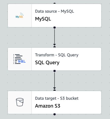
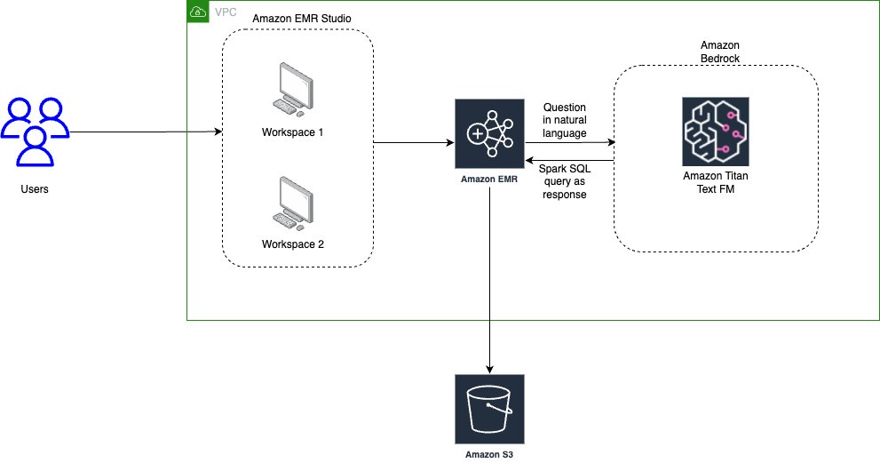
For this example, you use AWS Glue Studio to develop a visual ETL pipeline. This pipeline will read data from Amazon S3, perform transformations, and then load the transformed data into Teradata. The following diagram illustrates this architecture.

By the end of this post, your visual ETL job will resemble the following screenshot.

Prerequisites
For this example, you should have access to an existing Teradata database endpoint with network reachability from AWS and permissions to create tables and load and query data.
AWS Glue needs network access to Teradata to read or write data. How this is configured depends on where your Teradata is deployed and the specific network configuration. For Teradata deployed on AWS, you might need to configure VPC peering or AWS PrivateLink, security groups, and network access control lists (NACLs) to allow AWS Glue to communicate with Teradata overt TCP. If Teradata is outside AWS, networking services such as AWS Site-to-Site VPN or AWS Direct Connect may be required. Public internet access is not recommended due to security risks. If you choose public access, it’s safer to run the AWS Glue job in a VPC behind a NAT gateway. This approach enables you to allow list only one IP address for incoming traffic on your network firewall. For more information, refer to Infrastructure security in AWS Glue.
Set up Amazon S3
Every object in Amazon S3 is stored in a bucket. Before you can store data in Amazon S3, you must create an S3 bucket to store the results. Complete the following steps:
- On the Amazon S3 console, choose Buckets in the navigation pane.
- Choose Create bucket.
- For Name, enter a globally unique name for your bucket; for example, tickit8530923.
- Choose Create bucket.
- Download the TICKIT dataset and unzip it.
- Create the folder tickit in your S3 bucket and upload the allevents_pipe.txt and venue_pipe.txt files.
Configure Teradata connections
To connect to Teradata from AWS Glue, see Configuring Teradata Connection.
You must create and store your Teradata credentials in an AWS Secrets Manager secret and then associate that secret with a Teradata AWS Glue connection. We discuss these two steps in more detail later in this post.
Create an IAM role for the AWS Glue ETL job
When you create the AWS Glue ETL job, you specify an AWS Identity and Access Management (IAM) role for the job to use. The role must grant access to all resources used by the job, including Amazon S3 (for any sources, targets, scripts, driver files, and temporary directories) and Secrets Manager. For instructions, see Configure an IAM role for your ETL job.
Create table in Teradata
Using your preferred database tool, log in to Teradata. Run the following code to create the table in Teradata where you will load your data:
Store Teradata login credentials
An AWS Glue connection is a Data Catalog object that stores login credentials, URI strings, and more. The Teradata connector requires Secrets Manager for storing the Teradata user name and password that you use to connect to Teradata.
To store the Teradata user name and password in Secrets Manager, complete the following steps:
- On the Secrets Manager console, choose Secrets in the navigation pane.
- Choose Store a new secret.
- Select Other type of secret.
- Enter the key/value USER and
teradata_user, then choose Add row. - Enter the key/value PASSWORD and
teradata_user_password, then choose Next.

- For Secret name, enter a descriptive name, then choose Next.
- Choose Next to move to the review step, then choose Store.
Create the Teradata connection in AWS Glue
Now you’re ready to create an AWS Glue connection to Teradata. Complete the following steps:
- On the AWS Glue console, choose Connections under Data Catalog in the navigation pane.
- Choose Create connection.
- For Name, enter a name (for example,
teradata_connection). - For Connection type¸ choose Teradata.
- For Teradata URL, enter
jdbc:teradata://url_of_teradata/database=name_of_your_database. - For AWS Secret, choose the secret with your Teradata credentials that you created earlier.

Create an AWS Glue visual ETL job to transform and load data to Teradata
Complete the following steps to create your AWS Glue ETL job:
- On the AWS Glue console, under ETL Jobs in the navigation pane, choose Visual ETL.
- Choose Visual ETL.
- Choose the pencil icon to enter a name for your job.
We add venue_pipe.txt as our first dataset.
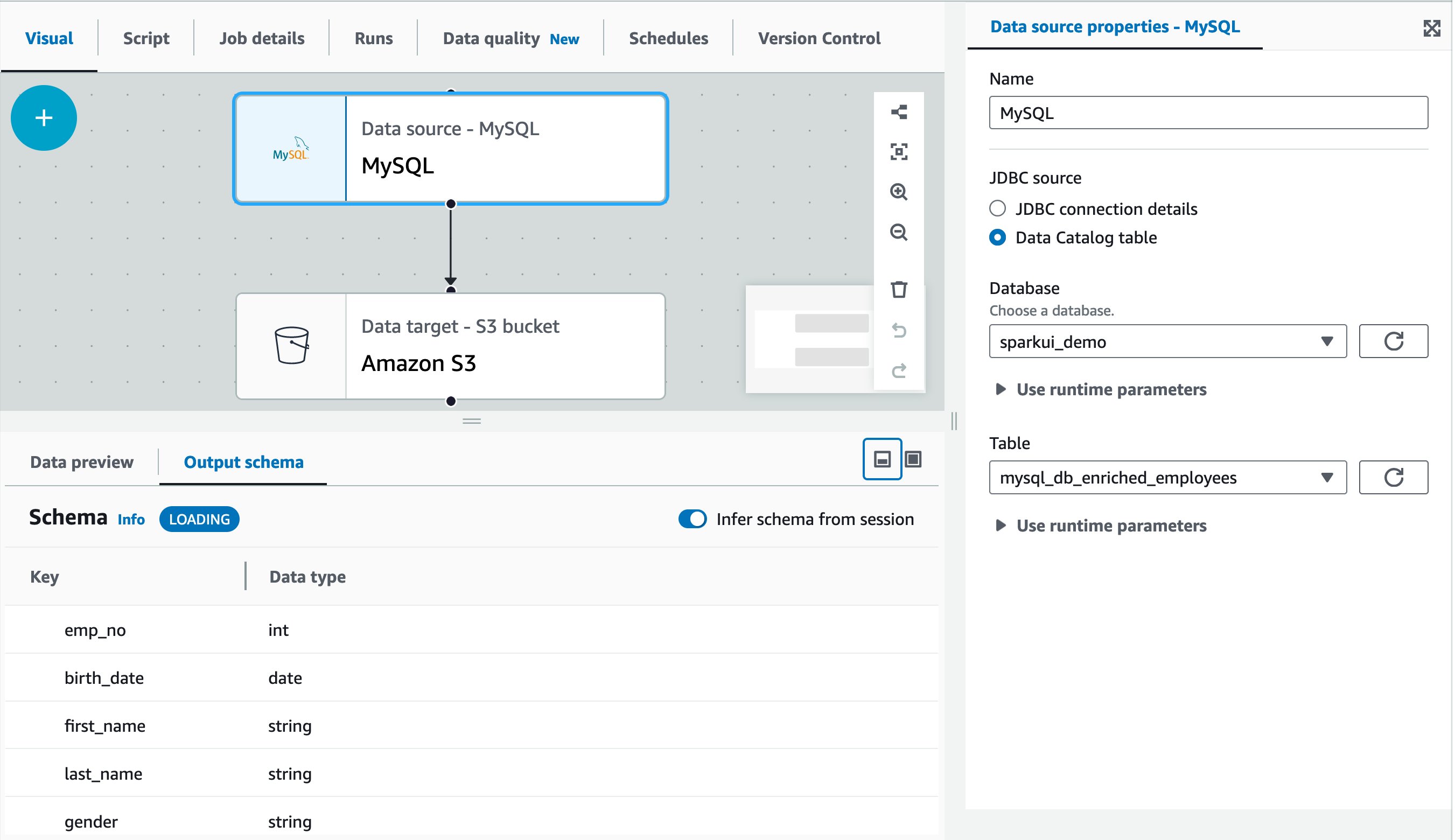
- Choose Add nodes and choose Amazon S3 on the Sources tab.

- Enter the following data source properties:
- For Name, enter Venue.
- For S3 source type, select S3 location.
- For S3 URL, enter the S3 path to
venue_pipe.txt. - For Data format, choose CSV.
- For Delimiter, choose Pipe.
- Deselect First line of source file contains column headers.

Now we add allevents_pipe.txt as our second dataset.
- Choose Add nodes and choose Amazon S3 on the Sources tab.
- Enter the following data source properties:
- For Name, enter Event.
- For S3 source type, select S3 location.
- For S3 URL, enter the S3 path to
allevents_pipe.txt. - For Data format, choose CSV.
- For Delimiter, choose Pipe.
- Deselect First line of source file contains column headers.
Next, we rename the columns of the Venue dataset.
- Choose Add nodes and choose Change Schema on the Transforms tab.
- Enter the following transform properties:
- For Name, enter Rename Venue data.
- For Node parents, choose Venue.
- In the Change Schema section, map the source keys to the target keys:
- col0:
venueid - col1:
venuename - col2:
venuecity - col3:
venuestate - col4:
venueseats
- col0:

Now we filter the Venue dataset to a specific geographic region.
- Choose Add nodes and choose Filter on the Transforms tab.
- Enter the following transform properties:
- For Name, enter Location Filter.
- For Node parents, choose Venue.
- For Filter condition, choose
venuestatefor Key, choose matches for Operation, and enter DC for Value.

Now we rename the columns in the Event dataset.
- Choose Add nodes and choose Change Schema on the Transforms tab.
- Enter the following transform properties:
- For Name, enter Rename Event data.
- For Node parents, choose Event.
- In the Change Schema section, map the source keys to the target keys:
- col0:
eventid - col1:
e_venueid - col2:
catid - col3:
dateid - col4:
eventname - col5:
starttime
- col0:
Next, we join the Venue and Event datasets.
- Choose Add nodes and choose Join on the Transforms tab.
- Enter the following transform properties:
- For Name, enter Join.
- For Node parents, choose Location Filter and Rename Event data.
- For Join type¸ choose Inner join.
- For Join conditions, choose
venueidfor Location Filter ande_venueidfor Rename Event data.

Now we drop the duplicate column.
- Choose Add nodes and choose Change Schema on the Transforms tab.
- Enter the following transform properties:
- For Name, enter Drop column.
- For Node parents, choose Join.
- In the Change Schema section, select Drop for
e_venueid.

Next, we load the data into the Teradata table.
- Choose Add nodes and choose Teradata on the Targets tab.
- Enter the following data sink properties:
- For Name, enter Teradata.
- For Node parents, choose Drop column.
- For Teradata connection, choose
teradata_connection. - For Table name, enter
schema.tablenameof the table you created in Teradata.

Lastly, we run the job and load the data into Teradata.
- Choose Save, then choose Run.
A banner will display that the job has started.
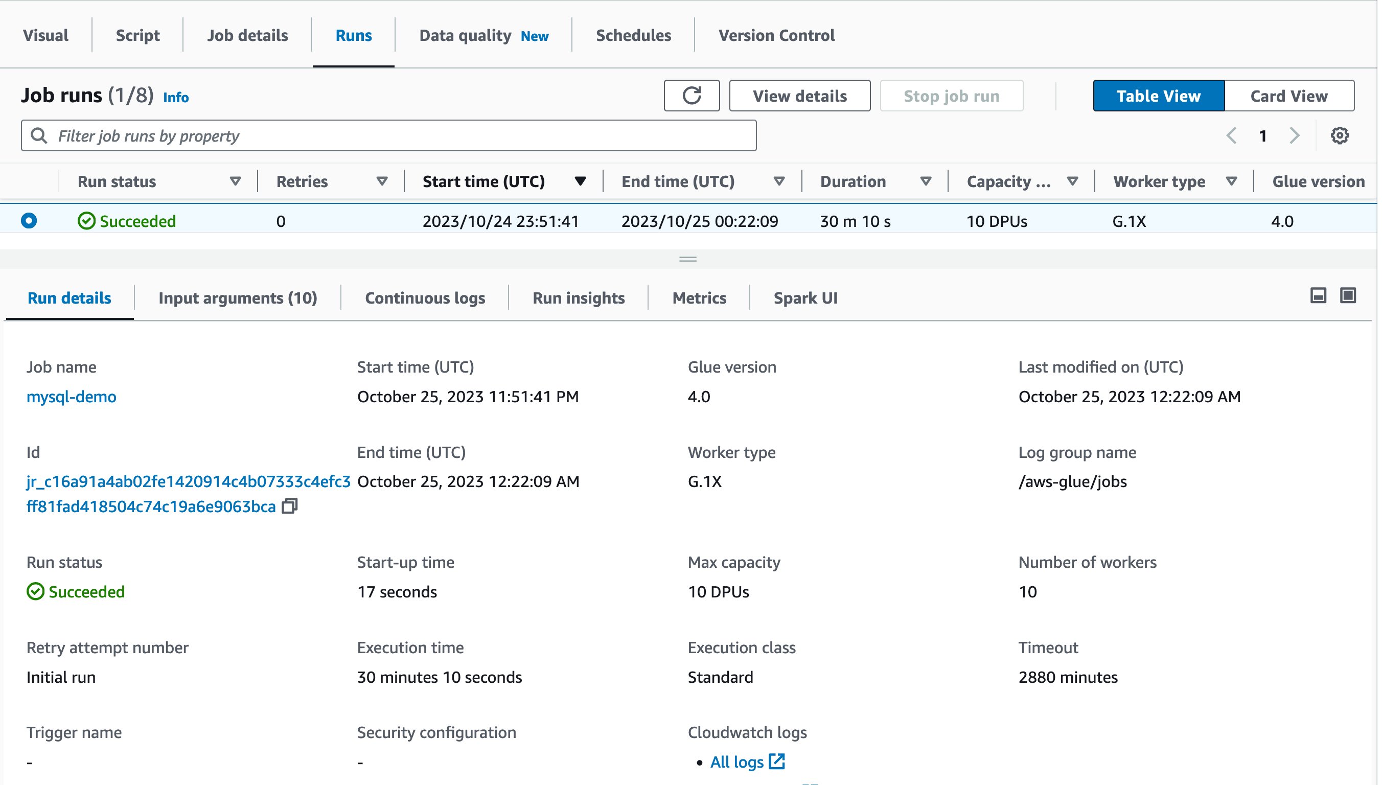
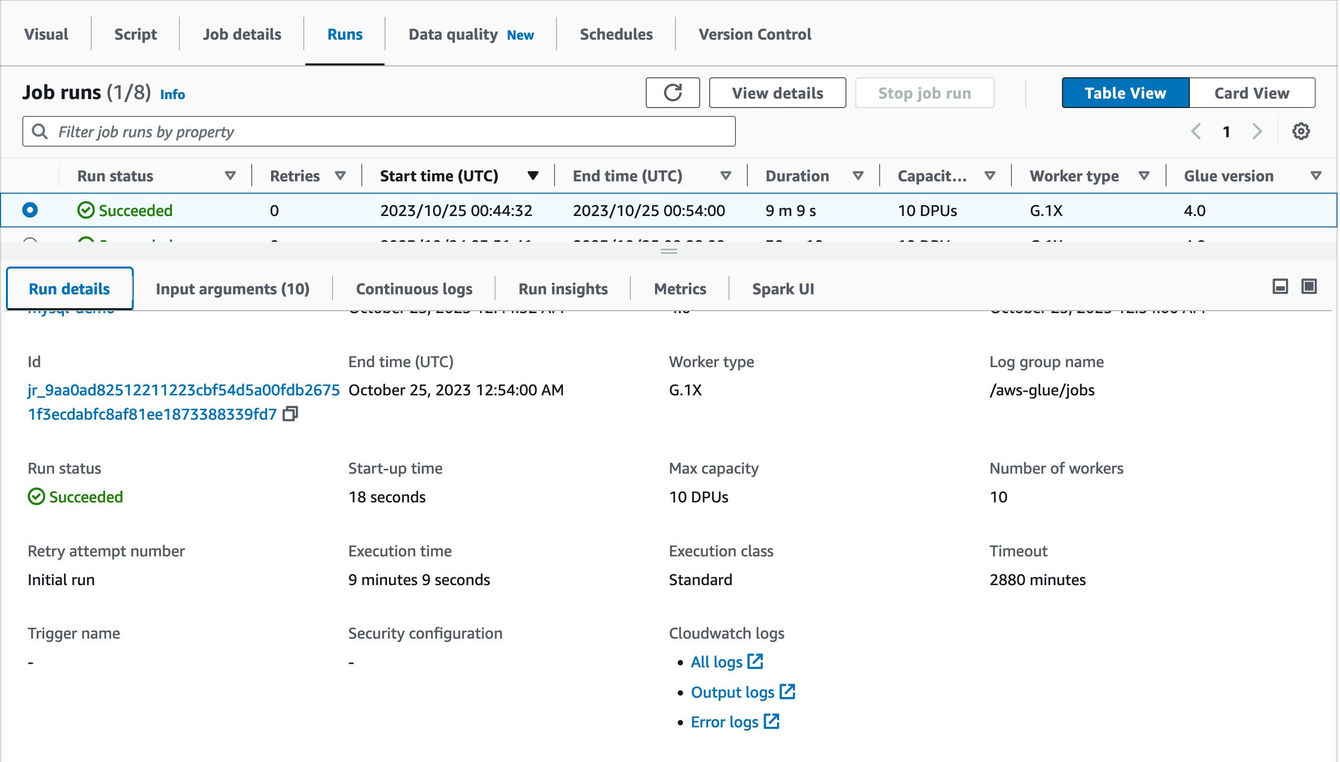
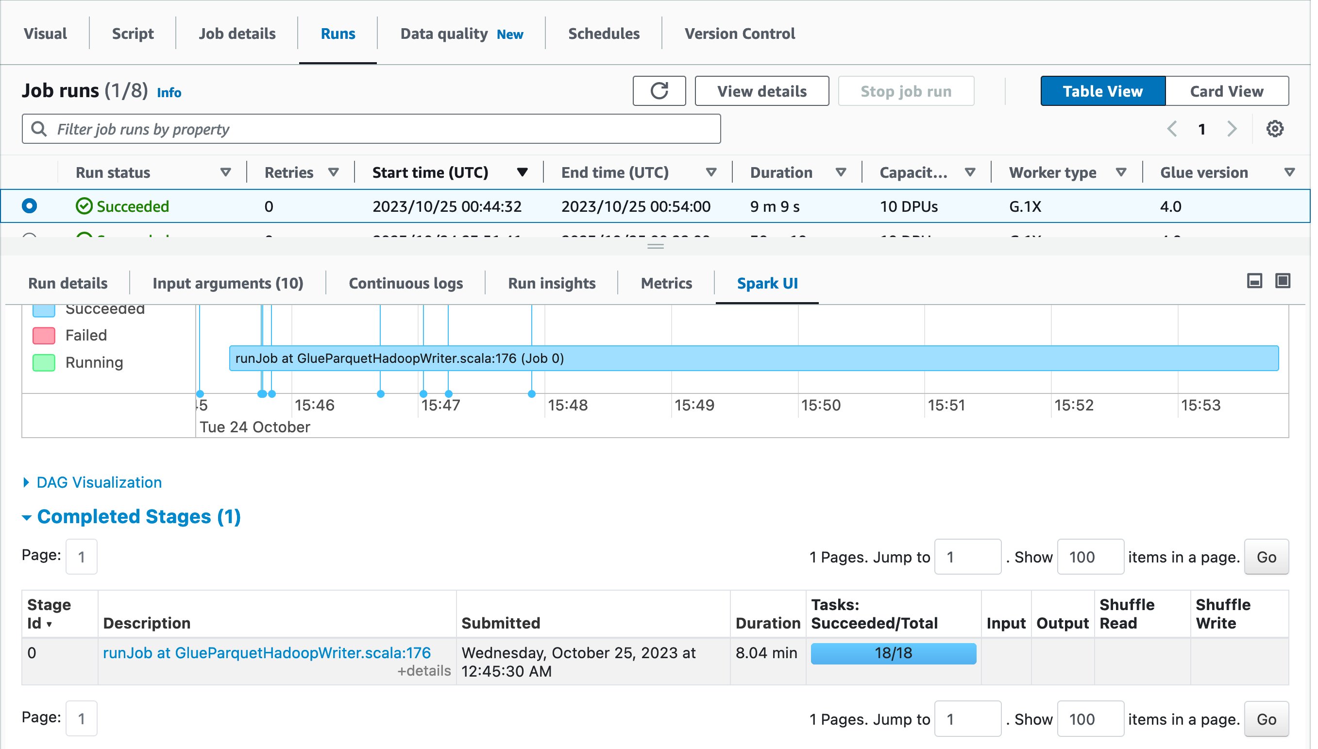
- Choose Runs, which displays the status of the job.
The run status will change to Succeeded when the job is complete.

- Connect to your Teradata and then query the table the data was loaded to it.
The filtered and joined data from the two datasets will be in the table.

Clean up
To avoid incurring additional charges caused by resources created as part of this post, make sure you delete the items you created in the AWS account for this post:
- The Secrets Manager key created for the Teradata credentials
- The AWS Glue native connector for Teradata Vantage
- The data loaded in the S3 bucket
- The AWS Glue Visual ETL job
Conclusion
In this post, you created a connection to Teradata using AWS Glue and then created an AWS Glue job to transform and load data into Teradata. The AWS Glue native connector for Teradata Vantage empowers your data analytics journey by providing a seamless and efficient pathway for integrating your data with Teradata. This new capability in AWS Glue not only simplifies your data integration workflows but also opens up new avenues for advanced analytics, business intelligence, and machine learning innovations.
With the AWS Teradata Connector, you have the best tool at your disposal for simplifying data integration tasks. Whether you’re looking to load Amazon S3 data into Teradata for analytics, reporting, or business insights, this new connector streamlines the process, making it more accessible and cost-effective.
To get started with AWS Glue, refer to Getting Started with AWS Glue.
About the Authors
 Kamen Sharlandjiev is a Sr. Big Data and ETL Solutions Architect and AWS Glue expert. He’s on a mission to make life easier for customers who are facing complex data integration challenges. His secret weapon? Fully managed, low-code AWS services that can get the job done with minimal effort and no coding. Follow Kamen on LinkedIn to keep up to date with the latest AWS Glue news!
 Sean Bjurstrom is a Technical Account Manager in ISV accounts at Amazon Web Services, where he specializes in analytics technologies and draws on his background in consulting to support customers on their analytics and cloud journeys. Sean is passionate about helping businesses harness the power of data to drive innovation and growth. Outside of work, he enjoys running and has participated in several marathons.
 Vinod Jayendra is an Enterprise Support Lead in ISV accounts at Amazon Web Services, where he helps customers solve their architectural, operational, and cost-optimization challenges. With a particular focus on serverless technologies, he draws from his extensive background in application development to help customers build top-tier solutions. Beyond work, he finds joy in quality family time, embarking on biking adventures, and coaching youth sports teams.
 Doug Mbaya is a Senior Partner Solution architect with a focus in analytics and machine learning. Doug works closely with AWS partners and helps them integrate their solutions with AWS analytics and machine learning solutions in the cloud.


 Noritaka Sekiyama is a Principal Big Data Architect on the AWS Glue team at Amazon Web Services. He works based in Tokyo, Japan. He is responsible for building software artifacts to help customers. In his spare time, he enjoys cycling with his road bike.
 Benjamin Menuet is a Senior Data Architect on the AWS Professional Services team at Amazon Web Services. He helps customers develop data and analytics solutions to accelerate their business outcomes. Outside of work, Benjamin is a trail runner and has finished some iconic races like the UTMB.
 Akira Ajisaka is a Senior Software Development Engineer on the AWS Glue team. He likes open source software and distributed systems. In his spare time, he enjoys playing arcade games.
 Kinshuk Pahare is a Principal Product Manager on the AWS Glue team at Amazon Web Services.
 Jason Ganz is the manager of the Developer Experience (DX) team at dbt Labs


 Sandeep Adwankar is a Senior Technical Product Manager at AWS. Based in the California Bay Area, he works with customers around the globe to translate business and technical requirements into products that enable customers to improve how they manage, secure, and access data.
 Navnit Shukla serves as an AWS Specialist Solution Architect with a focus on Analytics. He possesses a strong enthusiasm for assisting clients in discovering valuable insights from their data. Through his expertise, he constructs innovative solutions that empower businesses to arrive at informed, data-driven choices. Notably, Navnit Shukla is the accomplished author of the book titled Data Wrangling on AWS. He can be reached via


 Noritaka Sekiyama is a Principal Big Data Architect on the AWS Glue team. He works based in Tokyo, Japan. He is responsible for building software artifacts to help customers. In his spare time, he enjoys cycling with his road bike.
 Kyle Duong is a Software Development Engineer on the AWS Glue and Lake Formation team. He is passionate about building big data technologies and distributed systems.
 Sandeep Adwankar is a Senior Technical Product Manager at AWS. Based in the California Bay Area, he works with customers around the globe to translate business and technical requirements into products that enable customers to improve how they manage, secure, and access data.
 Shenoda Guirguis is a Senior Software Development Engineer on the AWS Glue team. His passion is in building scalable and distributed Data Infrastructure/Processing Systems. When he gets a chance, Shenoda enjoys reading and playing soccer.
 Sean Ma is a Principal Product Manager on the AWS Glue team. He has an 18+ year track record of innovating and delivering enterprise products that unlock the power of data for users. Outside of work, Sean enjoys scuba diving and college football.
 Mohit Saxena is a Senior Software Development Manager on the AWS Glue team. His team focuses on building distributed systems to enable customers with interactive and simple to use interfaces to efficiently manage and transform petabytes of data seamlessly across data lakes on Amazon S3, databases and data-warehouses on cloud.
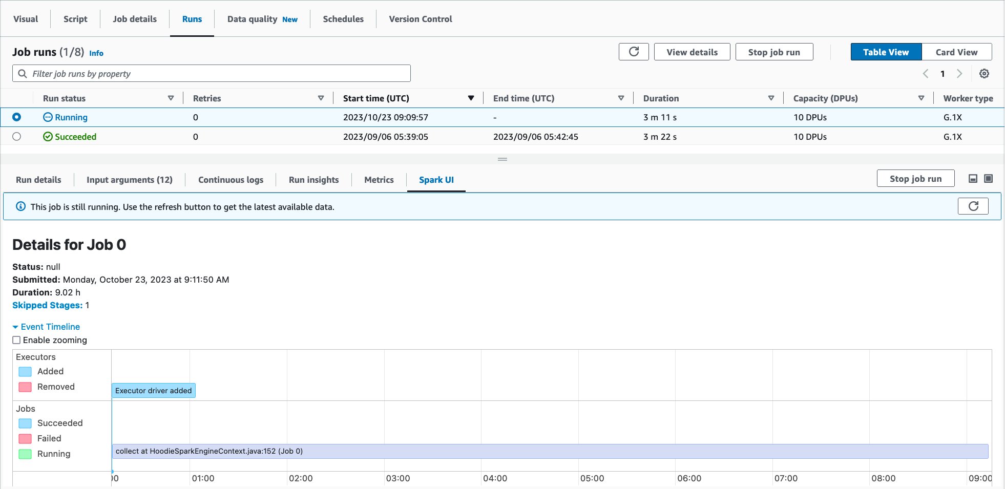

 Alexandra Tello is a Senior Front End Engineer with the AWS Glue team in New York City. She is a passionate advocate for usability and accessibility. In her free time, she’s an espresso enthusiast and enjoys building mechanical keyboards.
 Matt Sampson is a Software Development Manager on the AWS Glue team. He loves working with his other Glue team members to make services that our customers benefit from. Outside of work, he can be found fishing and maybe singing karaoke.
 Matt Su is a Senior Product Manager on the AWS Glue team. He enjoys helping customers uncover insights and make better decisions using their data with AWS Analytic services. In his spare time, he enjoys skiing and gardening.


 Saurabh Bhutyani is a Principal Analytics Specialist Solutions Architect at AWS. He is passionate about new technologies. He joined AWS in 2019 and works with customers to provide architectural guidance for running generative AI use cases, scalable analytics solutions and data mesh architectures using AWS services like Amazon Bedrock, Amazon SageMaker, Amazon EMR, Amazon Athena, AWS Glue, AWS Lake Formation, and Amazon DataZone.
 Harsh Vardhan is an AWS Senior Solutions Architect, specializing in analytics. He has over 8 years of experience working in the field of big data and data science. He is passionate about helping customers adopt best practices and discover insights from their data.


 Ismail Makhlouf is a Senior Specialist Solutions Architect for Data Analytics at AWS. Ismail focuses on architecting solutions for organizations across their end-to-end data analytics estate, including batch and real-time streaming, big data, data warehousing, and data lake workloads. He primarily works with direct-to-consumer platform companies in the ecommerce, FinTech, PropTech, and HealthTech space to achieve their business objectives with well-architected data platforms.


 Michael Hamilton is a Sr Analytics Solutions Architect focusing on helping enterprise customers in the south east modernize and simplify their analytics workloads on AWS. He enjoys mountain biking and spending time with his wife and three children when not working.
 Cody Penta is a Solutions Architect at Amazon Web Services and is based out of Charlotte, NC. He has a focus in security and CDK, and enjoys solving the really difficult problems in the technology world. Off the clock, he loves relaxing in the mountains, coding personal projects, and gaming.
 Angus Ferguson is a Solutions Architect at AWS who is passionate about meeting customers across the world, helping them solve their technical challenges. Angus specializes in Data & Analytics with a focus on customers in the financial services industry.


 Kartikay Khator is a Solutions Architect in Global Life Sciences at Amazon Web Services (AWS). He is passionate about building innovative and scalable solutions to meet the needs of customers, focusing on AWS Analytics services. Beyond the tech world, he is an avid runner and enjoys hiking.
 Kamen Sharlandjiev is a Sr. Big Data and ETL Solutions Architect and Amazon AppFlow expert. He’s on a mission to make life easier for customers who are facing complex data integration challenges. His secret weapon? Fully managed, low-code AWS services that can get the job done with minimal effort and no coding.
 Anshul Sharma is a Software Development Engineer in AWS Glue Team. He is driving the connectivity charter which provide Glue customer native way of connecting any Data source (Data-warehouse, Data-lakes, NoSQL etc) to Glue ETL Jobs. Beyond the tech world, he is a cricket and soccer lover.


 Anirban Sinha is a Senior Technical Account Manager at AWS. He is passionate about building scalable data warehouses and big data solutions working closely with customers. He works with large ISVs customers, in helping them build and operate secure, resilient, scalable, and high-performance SaaS applications in the cloud.
 Phil Bates is a Senior Analytics Specialist Solutions Architect at AWS. He has more than 25 years of experience implementing large-scale data warehouse solutions. He is passionate about helping customers through their cloud journey and using the power of ML within their data warehouse.
 Gaurav Singh is a Senior Solutions Architect at AWS, specializing in AI/ML and Generative AI. Based in Pune, India, he focuses on helping customers build, deploy, and migrate ML production workloads to SageMaker at scale. In his spare time, Gaurav loves to explore nature, read, and run.

 Sakti Mishra is a Principal Solutions Architect at AWS, where he helps customers modernize their data architecture and define their end-to-end data strategy, including data security, accessibility, governance, and more. He is also the author of the book
  Bhavana Chirumamilla is a Senior Resident Architect at AWS with a strong passion for data and machine learning operations. She brings a wealth of experience and enthusiasm to help enterprises build effective data and ML strategies. In her spare time, Bhavana enjoys spending time with her family and engaging in various activities such as traveling, hiking, gardening, and watching documentaries.
 Sheela Sonone is a Senior Resident Architect at AWS. She helps AWS customers make informed choices and trade-offs about accelerating their data, analytics, and AI/ML workloads and implementations. In her spare time, she enjoys spending time with her family—usually on tennis courts.
 Daniel Bruno is a Principal Resident Architect at AWS. He had been building analytics and machine learning solutions for over 20 years and splits his time helping customers build data science programs and designing impactful ML products.


 Qiushuang Feng is a Solutions Architect at AWS, responsible for Enterprise customers’ technical architecture design, consulting, and design optimization on AWS Cloud services. Before joining AWS, Qiushuang worked in IT companies such as IBM and Oracle, and accumulated rich practical experience in development and analytics.
 Shengjie Luo is a Big Data Architect on the Amazon Cloud Technology professional service team. They are responsible for solutions consulting, architecture, and delivery of AWS-based data warehouses and data lakes. They are skilled in serverless computing, data migration, cloud data integration, data warehouse planning, and data service architecture design and implementation.
 Greg Huang is a Senior Solutions Architect at AWS with expertise in technical architecture design and consulting for the China G1000 team. He is dedicated to deploying and utilizing enterprise-level applications on AWS Cloud services. He possesses nearly 20 years of rich experience in large-scale enterprise application development and implementation, having worked in the cloud computing field for many years. He has extensive experience in helping various types of enterprises migrate to the cloud. Prior to joining AWS, he worked for well-known IT enterprises such as Baidu and Oracle.
 Maciej Torbus is a Principal Customer Solutions Manager within Strategic Accounts at Amazon Web Services. With extensive experience in large-scale migrations, he focuses on helping customers move their applications and systems to highly reliable and scalable architectures in AWS. Outside of work, he enjoys sailing, traveling, and restoring vintage mechanical watches.


 Gokhul Srinivasan is a Senior Partner Solutions Architect leading AWS Healthcare and Life Sciences (HCLS) Global Startup Partners. Gokhul has over 19 years of Healthcare experience helping organizations with digital transformation, platform modernization, and deliver business outcomes.
 Laks Sundararajan is a seasoned Enterprise Architect helping companies reset, transform and modernize their IT, digital, cloud, data and insight strategies. A proven leader with significant expertise around Generative AI, Digital, Cloud and Data/Analytics Transformation, Laks is a Sr. Solutions Architect with Healthcare and Life Sciences (HCLS).
 Anil Chinnam is a Solutions Architect in the Digital Native Business Segment at Amazon Web Services(AWS). He enjoys working with customers to understand their challenges and solve them by creating innovative solutions using AWS services. Outside of work, Anil enjoys being a father, swimming and traveling.