Post Syndicated from Altaf Hussain original https://aws.amazon.com/blogs/big-data/build-an-amazon-redshift-data-warehouse-using-an-amazon-dynamodb-single-table-design/
Amazon DynamoDB is a fully managed NoSQL service that delivers single-digit millisecond performance at any scale. It’s used by thousands of customers for mission-critical workloads. Typical use cases for DynamoDB are an ecommerce application handling a high volume of transactions, or a gaming application that needs to maintain scorecards for players and games. In traditional databases, we would model such applications using a normalized data model (entity-relation diagram). This approach comes with a heavy computational cost in terms of processing and distributing the data across multiple tables while ensuring the system is ACID-compliant at all times, which can negatively impact performance and scalability. If these entities are frequently queried together, it makes sense to store them in a single table in DynamoDB. This is the concept of single-table design. Storing different types of data in a single table allows you to retrieve multiple, heterogeneous item types using a single request. Such requests are relatively straightforward, and usually take the following form:
SELECT * FROM TABLE WHERE Some_Attribute = 'some_value'
In this format, some_attribute is a partition key or part of an index.
Nonetheless, many of the same customers using DynamoDB would also like to be able to perform aggregations and ad hoc queries against their data to measure important KPIs that are pertinent to their business. Suppose we have a successful ecommerce application handling a high volume of sales transactions in DynamoDB. A typical ask for this data may be to identify sales trends as well as sales growth on a yearly, monthly, or even daily basis. These types of queries require complex aggregations over a large number of records. A key pillar of AWS’s modern data strategy is the use of purpose-built data stores for specific use cases to achieve performance, cost, and scale. Deriving business insights by identifying year-on-year sales growth is an example of an online analytical processing (OLAP) query. These types of queries are suited for a data warehouse.
The goal of a data warehouse is to enable businesses to analyze their data fast; this is important because it means they are able to gain valuable insights in a timely manner. Amazon Redshift is fully managed, scalable, cloud data warehouse. Building a performant data warehouse is non-trivial because the data needs to be highly curated to serve as a reliable and accurate version of the truth.
In this post, we walk through the process of exporting data from a DynamoDB table to Amazon Redshift. We discuss data model design for both NoSQL databases and SQL data warehouses. We begin with a single-table design as an initial state and build a scalable batch extract, load, and transform (ELT) pipeline to restructure the data into a dimensional model for OLAP workloads.
DynamoDB table example
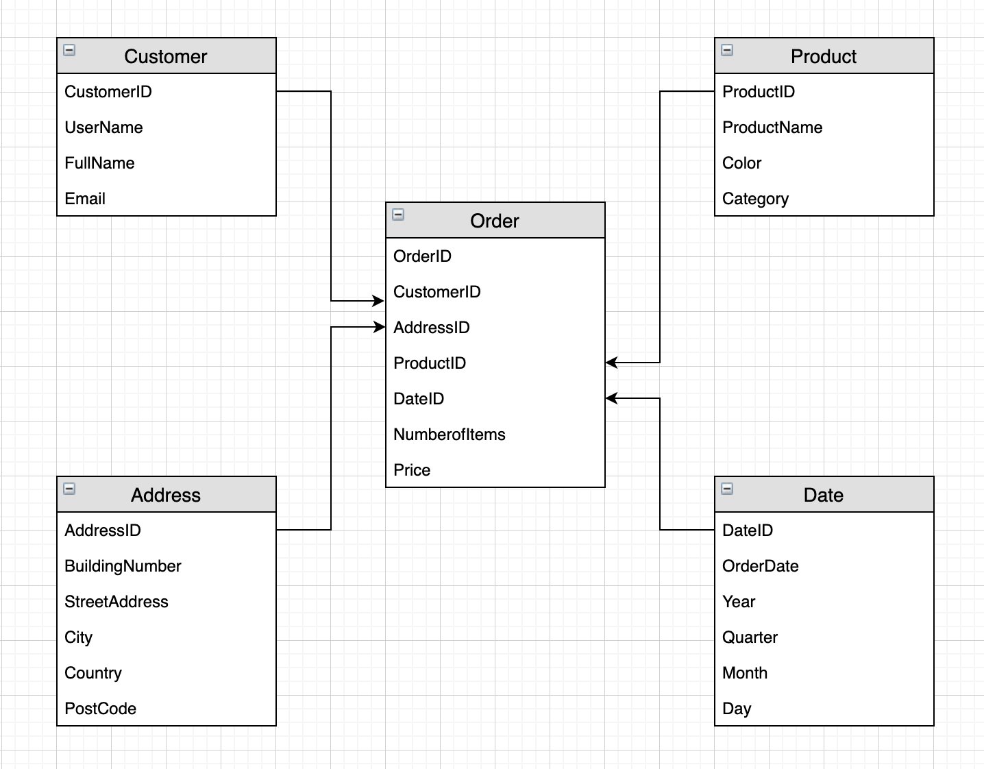
We use an example of a successful ecommerce store allowing registered users to order products from their website. A simple ERD (entity-relation diagram) for this application will have four distinct entities: customers, addresses, orders, and products. For customers, we have information such as their unique user name and email address; for the address entity, we have one or more customer addresses. Orders contain information regarding the order placed, and the products entity provides information about the products placed in an order. As we can see from the following diagram, a customer can place one or more orders, and an order must contain one or more products.

We could store each entity in a separate table in DynamoDB. However, there is no way to retrieve customer details alongside all the orders placed by the customer without making multiple requests to the customer and order tables. This is inefficient from both a cost and performance perspective. A key goal for any efficient application is to retrieve all the required information in a single query request. This ensures fast, consistent performance. So how can we remodel our data to avoid making multiple requests? One option is to use single-table design. Taking advantage of the schema-less nature of DynamoDB, we can store different types of records in a single table in order to handle different access patterns in a single request. We can go further still and store different types of values in the same attribute and use it as a global secondary index (GSI). This is called index overloading.
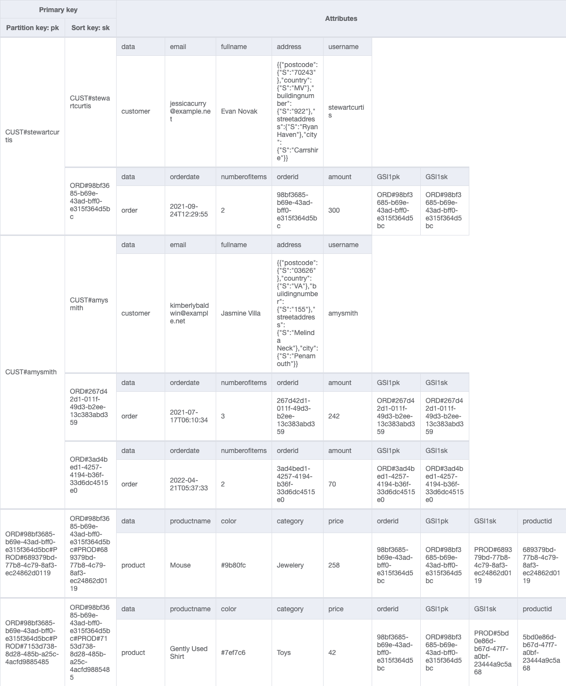
A typical access pattern we may want to handle in our single table design is to get customer details and all orders placed by the customer.
To accommodate this access pattern, our single-table design looks like the following example.

By restricting the number of addresses associated with a customer, we can store address details as a complex attribute (rather than a separate item) without exceeding the 400 KB item size limit of DynamoDB.
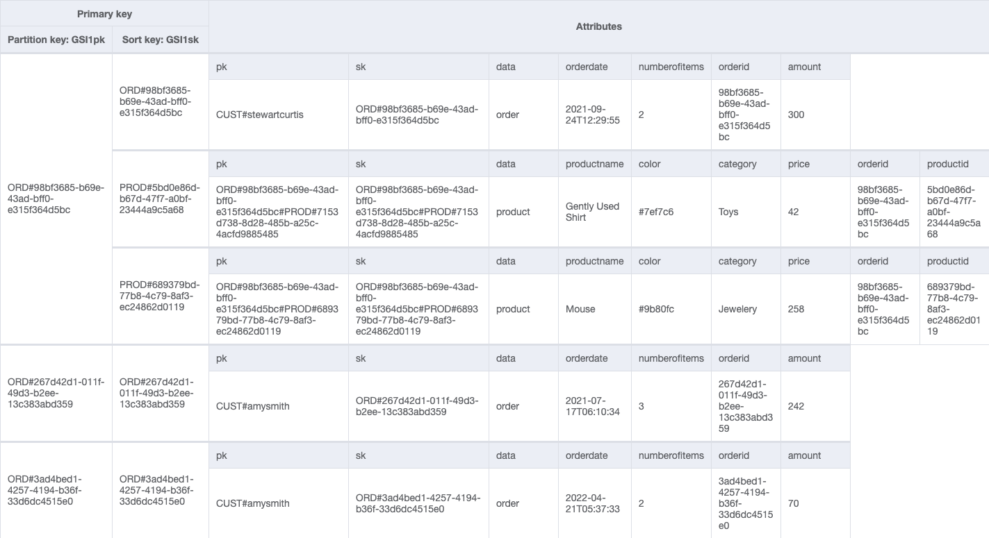
We can add a global secondary index (GSIpk and GSIsk) to capture another access pattern: get order details and all product items placed in an order. We use the following table.

We have used generic attribute names, PK and SK, for our partition key and sort key columns. This is because they hold data from different entities. Furthermore, the values in these columns are prefixed by generic terms such as CUST# and ORD# to help us identify the type of data we have and ensure that the value in PK is unique across all records in the table.
A well-designed single table will not only reduce the number of requests for an access pattern, but will service many different access patterns. The challenge comes when we need to ask more complex questions of our data, for example, what was the year-on-year quarterly sales growth by product broken down by country?
The case for a data warehouse
A data warehouse is ideally suited to answer OLAP queries. Built on highly curated structured data, it provides the flexibility and speed to run aggregations across an entire dataset to derive insights.
To house our data, we need to define a data model. An optimal design choice is to use a dimensional model. A dimension model consists of fact tables and dimension tables. Fact tables store the numeric information about business measures and foreign keys to the dimension tables. Dimension tables store descriptive information about the business facts to help understand and analyze the data better. From a business perspective, a dimension model with its use of facts and dimensions can present complex business processes in a simple-to-understand manner.
Building a dimensional model
A dimensional model optimizes read performance through efficient joins and filters. Amazon Redshift automatically chooses the best distribution style and sort key based on workload patterns. We build a dimensional model from the single DynamoDB table based on the following star schema.

We have separated each item type into individual tables. We have a single fact table (Orders) containing the business measures price and numberofitems, and foreign keys to the dimension tables. By storing the price of each product in the fact table, we can track price fluctuations in the fact table without continually updating the product dimension. (In a similar vein, the DynamoDB attribute amount is a simple derived measure in our star schema: amount is the summation of product prices per orderid).
By splitting the descriptive content of our single DynamoDB table into multiple Amazon Redshift dimension tables, we can remove redundancy by only holding in each dimension the information pertinent to it. This allows us the flexibility to query the data under different contexts; for example, we may want to know the frequency of customer orders by city or product sales by date. The ability to freely join dimensions and facts when analyzing the data is one of the key benefits of dimensional modeling. It’s also good practice to have a Date dimension to allow us to perform time-based analysis by aggregating the fact by year, month, quarter, and so forth.
This dimensional model will be built in Amazon Redshift. When setting out to build a data warehouse, it’s a common pattern to have a data lake as the source of the data warehouse. The data lake in this context serves a number of important functions:
- It acts as a central source for multiple applications, not just exclusively for data warehousing purposes. For example, the same dataset could be used to build machine learning (ML) models to identify trends and predict sales.
- It can store data as is, be it unstructured, semi-structured, or structured. This allows you to explore and analyze the data without committing upfront to what the structure of the data should be.
- It can be used to offload historical or less-frequently-accessed data, allowing you to manage your compute and storage costs more effectively. In our analytic use case, if we are analyzing quarterly growth rates, we may only need a couple of years’ worth of data; the rest can be unloaded into the data lake.
When querying a data lake, we need to consider user access patterns in order to reduce costs and optimize query performance. This is achieved by partitioning the data. The choice of partition keys will depend on how you query the data. For example, if you query the data by customer or country, then they are good candidates for partition keys; if you query by date, then a date hierarchy can be used to partition the data.
After the data is partitioned, we want to ensure it’s held in the right format for optimal query performance. The recommended choice is to use a columnar format such as Parquet or ORC. Such formats are compressed and store data column-wise, allowing for fast retrieval times, and are parallelizable, allowing for fast load times when moving the data into Amazon Redshift. In our use case, it makes sense to store the data in a data lake with minimal transformation and formatting to enable easy querying and exploration of the dataset. We partition the data by item type (Customer, Order, Product, and so on), and because we want to easily query each entity in order to move the data into our data warehouse, we transform the data into the Parquet format.
Solution overview
The following diagram illustrates the data flow to export data from a DynamoDB table to a data warehouse.

We present a batch ELT solution using AWS Glue for exporting data stored in DynamoDB to an Amazon Simple Storage Service (Amazon S3) data lake and then a data warehouse built in Amazon Redshift. AWS Glue is a fully managed extract, transform, and load (ETL) service that allows you to organize, cleanse, validate, and format data for storage in a data warehouse or data lake.
The solution workflow has the following steps:
- Move any existing files from the raw and data lake buckets into corresponding archive buckets to ensure any fresh export from DynamoDB to Amazon S3 isn’t duplicating data.
- Begin a new DynamoDB export to the S3 raw layer.
- From the raw files, create a data lake partitioned by item type.
- Load the data from the data lake to landing tables in Amazon Redshift.
- After the data is loaded, we take advantage of the distributed compute capability of Amazon Redshift to transform the data into our dimensional model and populate the data warehouse.
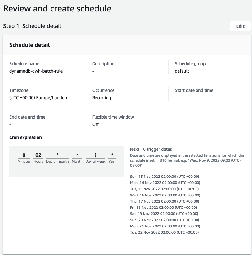
We orchestrate the pipeline using an AWS Step Functions workflow and schedule a daily batch run using Amazon EventBridge.
For simpler DynamoDB table structures you may consider skipping some of these steps by either loading data directly from DynamoDB to Redshift or using Redshift’s auto-copy or copy command to load data from S3.
Prerequisites
You must have an AWS account with a user who has programmatic access. For setup instructions, refer to AWS security credentials.
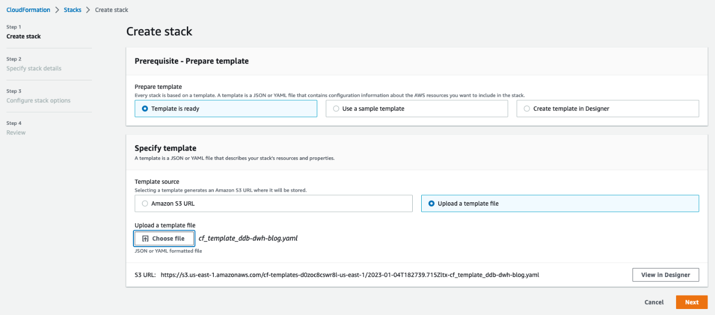
Use the AWS CloudFormation template cf_template_ddb-dwh-blog.yaml to launch the following resources:
- A DynamoDB table with a GSI and point-in-time recovery enabled.
- An Amazon Redshift cluster (we use two nodes of RA3.4xlarge).
- Three AWS Glue database catalogs:
raw, datalake, and redshift.
- Five S3 buckets: two for the raw and data lake files; two for their respective archives, and one for the Amazon Athena query results.
- Two AWS Identity and Access Management (IAM) roles: An AWS Glue role and a Step Functions role with the requisite permissions and access to resources.
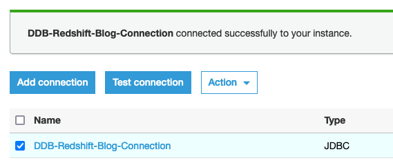
- A JDBC connection to Amazon Redshift.
- An AWS Lambda function to retrieve the
s3-prefix-list-id for your Region. This is required to allow traffic from a VPC to access an AWS service through a gateway VPC endpoint.
- Download the following files to perform the ELT:
- The Python script to load sample data into our DynamoDB table: load_dynamodb.py.
- The AWS Glue Python Spark script to archive the raw and data lake files: archive_job.py.
- The AWS Glue Spark scripts to extract and load the data from DynamoDB to Amazon Redshift: GlueSparkJobs.zip.
- The DDL and DML SQL scripts to create the tables and load the data into the data warehouse in Amazon Redshift: SQL Scripts.zip.
Launch the CloudFormation template
AWS CloudFormation allows you to model, provision, and scale your AWS resources by treating infrastructure as code. We use the downloaded CloudFormation template to create a stack (with new resources).
- On the AWS CloudFormation console, create a new stack and select Template is ready.
- Upload the stack and choose Next.

- Enter a name for your stack.
- For MasterUserPassword, enter a password.
- Optionally, replace the default names for the Amazon Redshift database, DynamoDB table, and MasterUsername (in case these names are already in use).
- Reviewed the details and acknowledge that AWS CloudFormation may create IAM resources on your behalf.
- Choose Create stack.
Load sample data into a DynamoDB table
To load your sample data into DynamoDB, complete the following steps:
- Create an AWS Cloud9 environment with default settings.
- Upload the load DynamoDB Python script. From the AWS Cloud9 terminal, use the pip install command to install the following packages:
boto3fakerfaker_commercenumpy
- In the Python script, replace all placeholders (capital letters) with the appropriate values and run the following command in the terminal:
This command loads the sample data into our single DynamoDB table.
Extract data from DynamoDB
To extract the data from DynamoDB to our S3 data lake, we use the new AWS Glue DynamoDB export connector. Unlike the old connector, the new version uses a snapshot of the DynamoDB table and doesn’t consume read capacity units of your source DynamoDB table. For large DynamoDB tables exceeding 100 GB, the read performance of the new AWS Glue DynamoDB export connector is not only consistent but also significantly faster than the previous version.
To use this new export connector, you need to enable point-in-time recovery (PITR) for the source DynamoDB table in advance. This will take continuous backups of the source table (so be mindful of cost) and ensures that each time the connector invokes an export, the data is fresh. The time it takes to complete an export depends on the size of your table and how uniformly the data is distributed therein. This can range from a few minutes for small tables (up to 10 GiB) to a few hours for larger tables (up to a few terabytes). This is not a concern for our use case because data lakes and data warehouses are typically used to aggregate data at scale and generate daily, weekly, or monthly reports. It’s also worth noting that each export is a full refresh of the data, so in order to build a scalable automated data pipeline, we need to archive the existing files before beginning a fresh export from DynamoDB.
Complete the following steps:
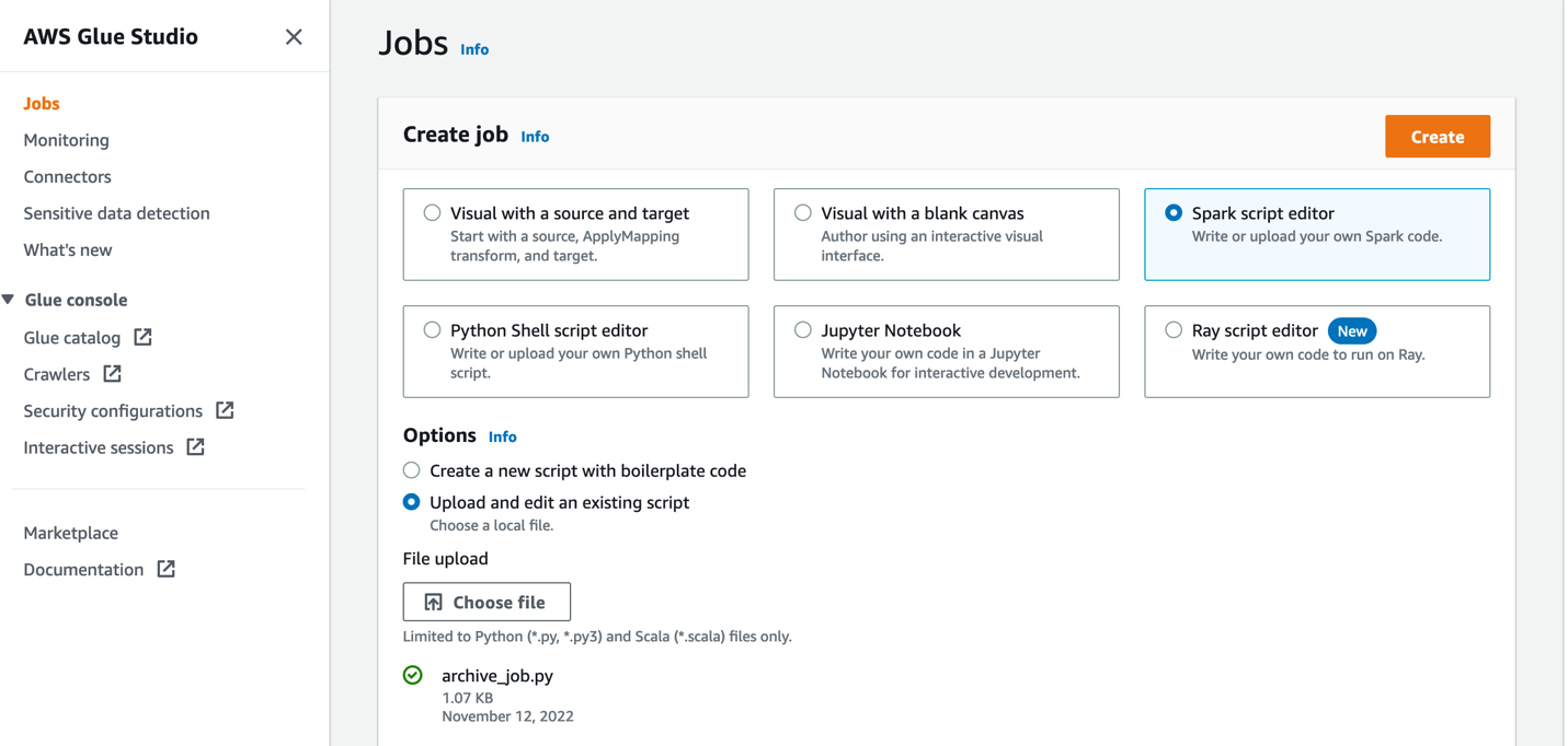
- Create an AWS Glue job using the Spark script editor.
- Upload the
archive_job.py file from GlueSparkJobs.zip.
This job archives the data files into timestamped folders. We run the job concurrently to archive the raw files and the data lake files.

- In Job details section, give the job a name and choose the AWS Glue IAM role created by our CloudFormation template.
- Keep all defaults the same and ensure maximum concurrency is set to 2 (under Advanced properties).
Archiving the files provides a backup option in the event of disaster recovery. As such, we can assume that the files will not be accessed frequently and can be kept in Standard_IA storage class so as to save up to 40% on costs while providing rapid access to the files when needed.
This job typically runs before each export of data from DynamoDB. After the datasets have been archived, we’re ready to (re)-export the data from our DynamoDB table.
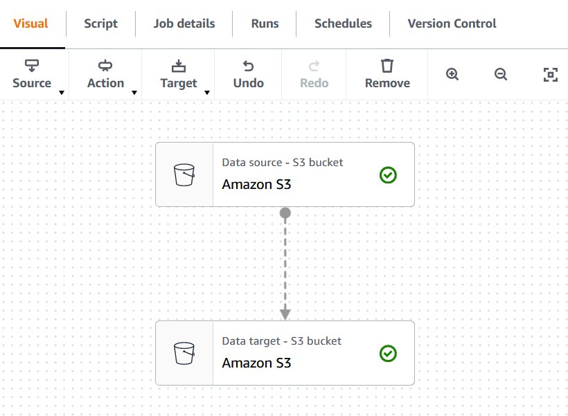
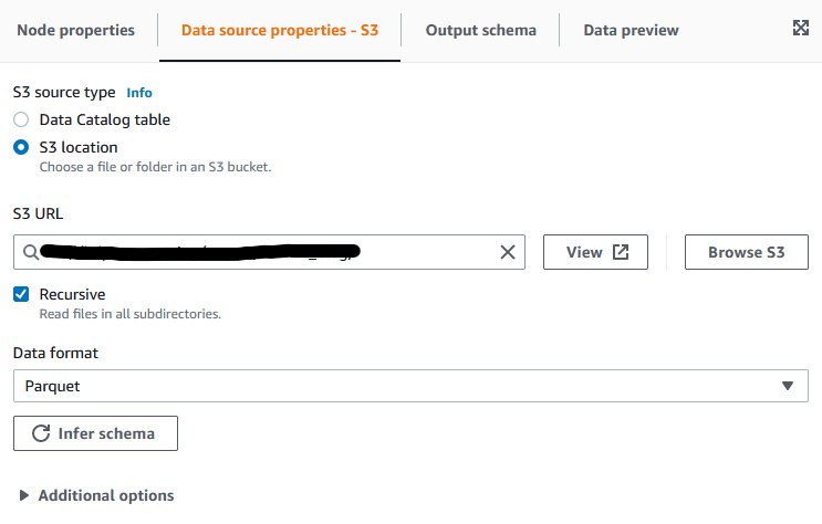
We can use AWS Glue Studio to visually create the jobs needed to extract the data from DynamoDB and load into our Amazon Redshift data warehouse. We demonstrate how to do this by creating an AWS Glue job (called ddb_export_raw_job) using AWS Glue Studio.
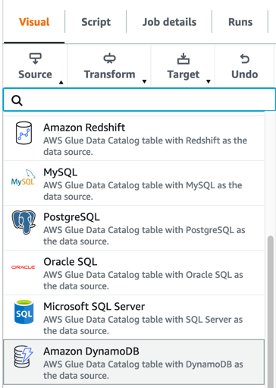
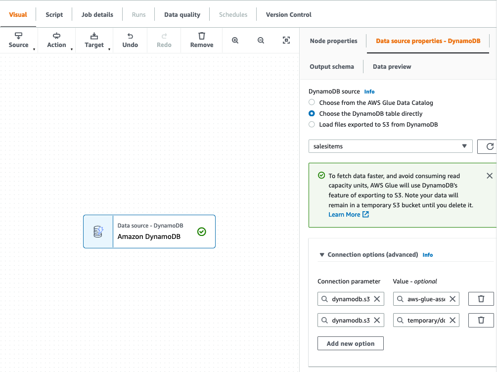
- In AWS Glue Studio, create a job and select Visual with a blank canvas.
- Choose Amazon DynamoDB as the data source.

- Choose our DynamoDB table to export from.
- Leave all other options as is and finish setting up the source connection.

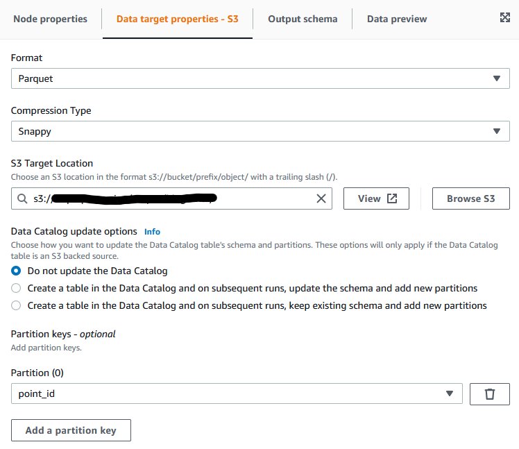
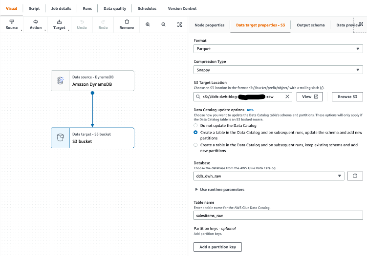
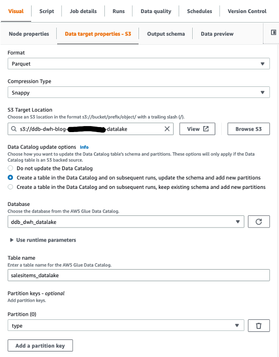
We then choose Amazon S3 as our target. In the target properties, we can transform the output to a suitable format, apply compression, and specify the S3 location to store our raw data.
- Set the following options:
- For Format, choose Parquet.
- For Compression type, choose Snappy.
- For S3 Target Location, enter the path for
RawBucket (located on the Outputs tab of the CloudFormation stack).
- For Database, choose the value for
GlueRawDatabase (from the CloudFormation stack output).
- For Table name, enter an appropriate name.

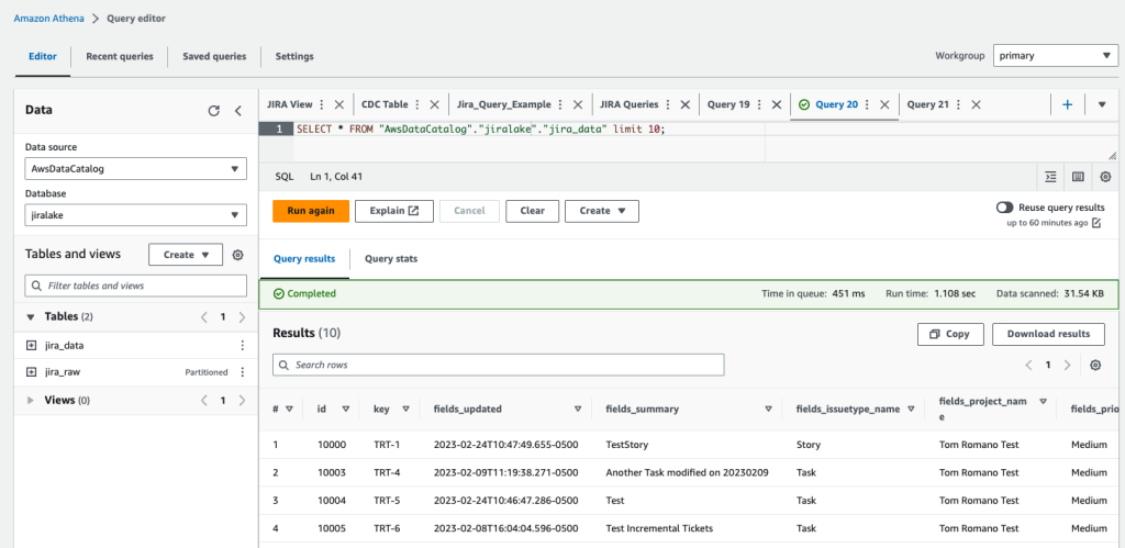
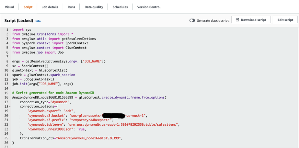
- Because our target data warehouse requires data to be in a flat structure, verify that the configuration option
dynamodb.unnestDDBJson is set to True on the Script tab.

- On the Job details tab, choose the AWS Glue IAM role generated by the CloudFormation template.
- Save and run the job.
Depending on the data volumes being exported, this job may take a few minutes to complete.
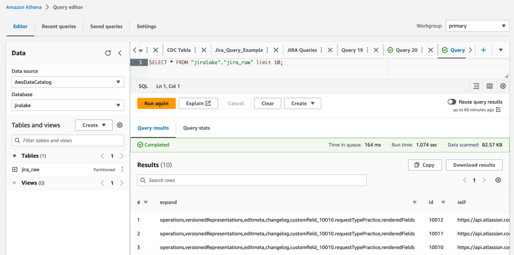
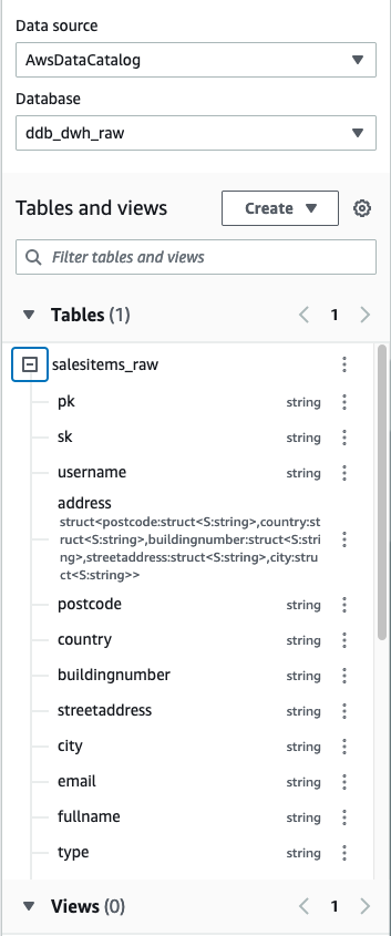
Because we’ll be adding the table to our AWS Glue Data Catalog, we can explore the output using Athena after the job is complete. Athena is a serverless interactive query service that makes it simple to analyze data directly in Amazon S3 using standard SQL.
- In the Athena query editor, choose the raw database.
We can see that the attributes of the Address structure have been unnested and added as additional columns to the table.

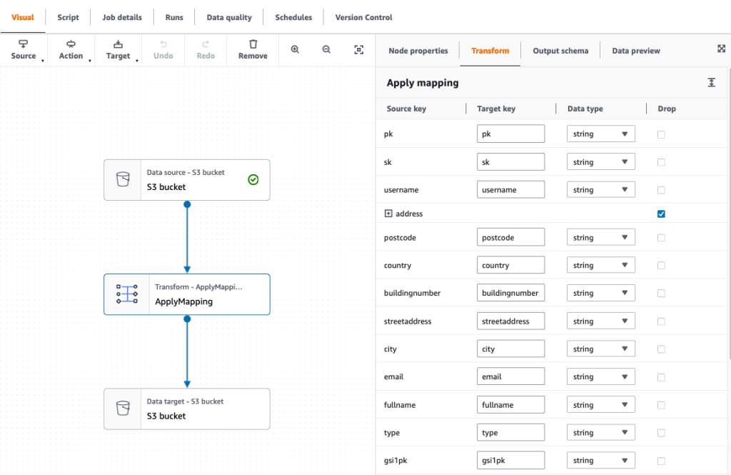
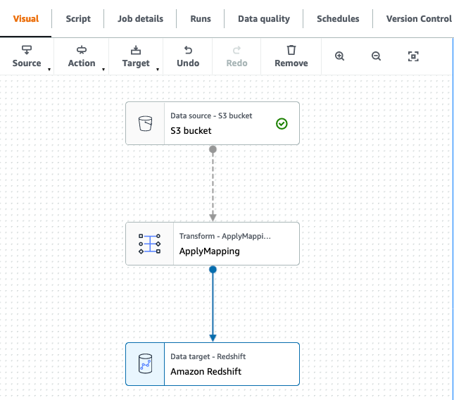
- After we export the data into the raw bucket, create another job (called
raw_to_datalake_job) using AWS Glue Studio (select Visual with a blank canvas) to load the data lake partitioned by item type (customer, order, and product).
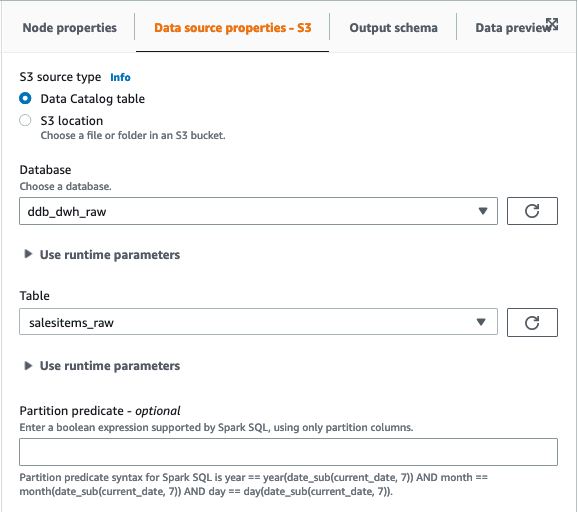
- Set the source as the AWS Glue Data Catalog raw database and table.

- In the ApplyMapping transformation, drop the Address struct because we have already unnested these attributes into our flattened raw table.

- Set the target as our S3 data lake.

- Choose the AWS Glue IAM role in the job details, then save and run the job.
Now that we have our data lake, we’re ready to build our data warehouse.
Build the dimensional model in Amazon Redshift
The CloudFormation template launches a two-node RA3.4xlarge Amazon Redshift cluster. To build the dimensional model, complete the following steps:
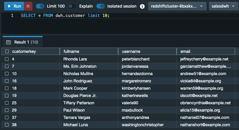
- In Amazon Redshift Query Editor V2, connect to your database (default:
salesdwh) within the cluster using the database user name and password authentication (MasterUserName and MasterUserPassword from the CloudFormation template).
- You may be asked to configure your account if this is your first time using Query Editor V2.
- Download the SQL scripts SQL Scripts.zip to create the following schemas and tables (run the scripts in numbered sequence).
In the landing schema:
addresscustomerorderproduct
In the staging schema:
staging.addressstaging.address_maxkeystaging.addresskeystaging.customerstaging.customer_maxkeystaging.customerkeystaging.datestaging.date_maxkeystaging.datekeystaging.orderstaging.order_maxkeystaging.orderkeystaging.productstaging.product_maxkeystaging.productkey
In the dwh schema:
dwh.addressdwh.customerdwh.orderdwh.product
We load the data from our data lake to the landing schema as is.
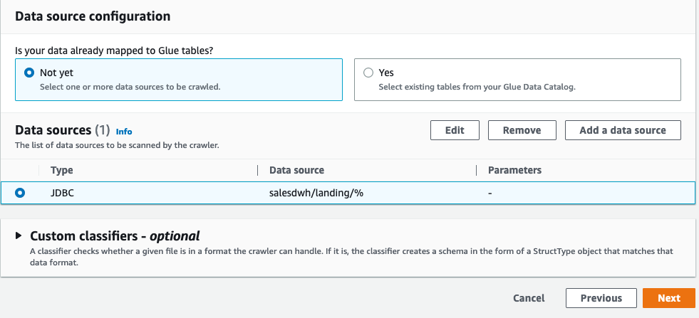
- Use the JDBC connector to Amazon Redshift to build an AWS Glue crawler to add the landing schema to our Data Catalog under the
ddb_redshift database.

- Create an AWS Glue crawler with the JDBC data source.

- Select the JDBC connection you created and choose Next.

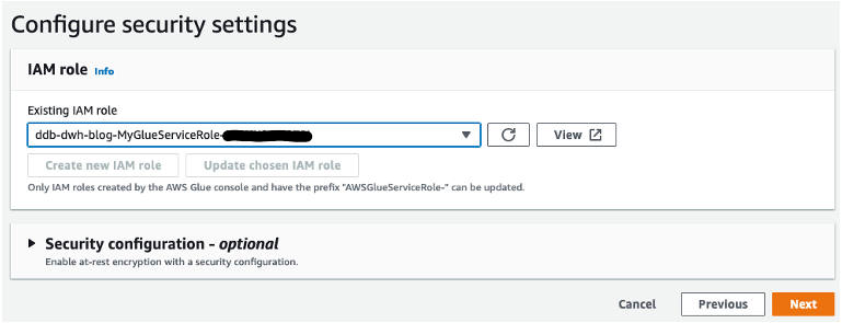
- Choose the IAM role created by the CloudFormation template and choose Next.

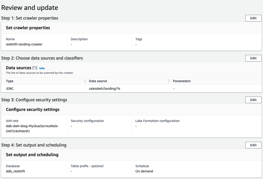
- Review your settings before creating the crawler.

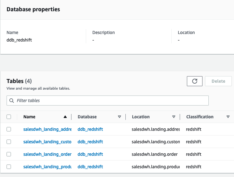
The crawler adds the four landing tables in our AWS Glue database ddb_redshift.

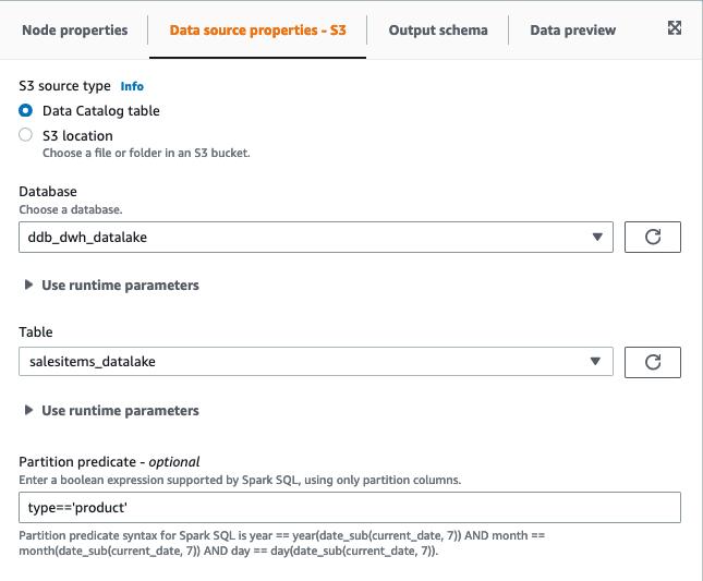
- In AWS Glue Studio, create four AWS Glue jobs to load the landing tables (these scripts are available to download, and you can use the Spark script editor to upload these scripts individually to create the jobs):
land_order_jobland_product_jobland_customer_jobland_address_job
Each job has the structure as shown in the following screenshot.

- Filter the S3 source on the partition column type:
- For
product, filter on type=‘product’.
- For
order, filter on type=‘order’.
- For
customer and address, filter on type=‘customer’.

- Set the target for the data flow as the corresponding table in the
landing schema in Amazon Redshift.
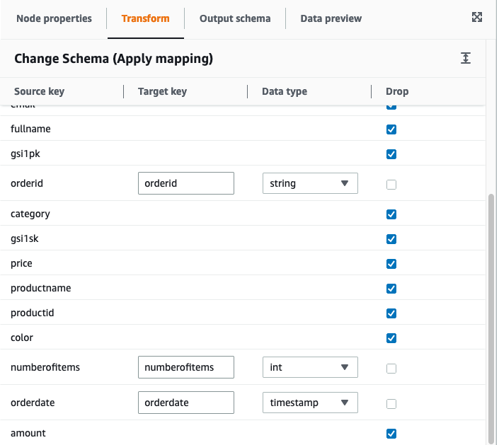
- Use the built-in
ApplyMapping transformation in our data pipeline to drop columns and, where necessary, convert the data types to match the target columns.
For more information about built-in transforms available in AWS Glue, refer to AWS Glue PySpark transforms reference.

The mappings for our four jobs are as follows:
land_order_job:
mappings=[
("pk", "string", "pk", "string"),
("orderid", "string", "orderid", "string"),
("numberofitems", "string", "numberofitems", "int"),
("orderdate", "string", "orderdate", "timestamp"),
]
land_product_job:
mappings=[
("orderid", "string", "orderid", "string"),
("category", "string", "category", "string"),
("price", "string", "price", "decimal"),
("productname", "string", "productname", "string"),
("productid", "string", "productid", "string"),
("color", "string", "color", "string"),
]
land_address_job:
mappings=[
("username", "string", "username", "string"),
("email", "string", "email", "string"),
("fullname", "string", "fullname", "string"),
]
land_customer_job:
mappings=[
("username", "string", "username", "string"),
("email", "string", "email", "string"),
("fullname", "string", "fullname", "string"),
]
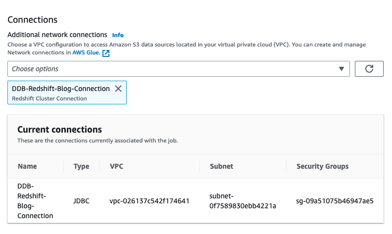
- Choose the AWS Glue IAM role, and under Advanced properties, verify the JDBC connector to Amazon Redshift as a connection.
- Save and run each job to load the landing tables in Amazon Redshift.

Populate the data warehouse
From the landing schema, we move the data to the staging layer and apply the necessary transformations. Our dimensional model has a single fact table, the orders table, which is the largest table and as such needs a distribution key. The choice of key depends on how the data is queried and the size of the dimension tables being joined to. If you’re unsure of your query patterns, you can leave the distribution keys and sort keys for your tables unspecified. Amazon Redshift automatically assigns the correct distribution and sort keys based on your queries. This has the advantage that if and when query patterns change over time, Amazon Redshift can automatically update the keys to reflect the change in usage.
In the staging schema, we keep track of existing records based on their business key (the unique identifier for the record). We create key tables to generate a numeric identity column for each table based on the business key. These key tables allow us to implement an incremental transformation of the data into our dimensional model.
CREATE TABLE IF NOT EXISTS staging.productkey (
    productkey integer identity(1,1),
    productid character varying(16383),
    CONSTRAINT products_pkey PRIMARY KEY(productkey));
When loading the data, we need to keep track of the latest surrogate key value to ensure that new records are assigned the correct increment. We do this using maxkey tables (pre-populated with zero):
CREATE TABLE IF NOT EXISTS staging.product_maxkey (
    productmaxkey integer);

INSERT INTO staging.product_maxkey
select 0;
We use staging tables to store our incremental load, the structure of which will mirror our final target model in the dwh schema:
---staging tables to load data from data lake

CREATE TABLE IF NOT EXISTS staging.product (
    productkey integer,
    productname character varying(200),
    color character varying(50),
    category character varying(100),
    PRIMARY KEY (productkey));
---dwh tables to load data from staging schema

CREATE TABLE IF NOT EXISTS dwh.product (
    productkey integer,
    productname character varying(200),
    color character varying(50),
    category character varying(100),
    PRIMARY KEY (productkey));
Incremental processing in the data warehouse
We load the target data warehouse using stored procedures to perform upserts (deletes and inserts performed in a single transaction):
CREATE OR REPLACE PROCEDURE staging.load_order() LANGUAGE plpgsql AS $$
DECLARE
BEGIN

TRUNCATE TABLE staging.order;

--insert new records to get new ids
insert into staging.orderkey
(
orderid
)
select
c.orderid
from landing.order c
LEFT JOIN staging.orderkey i
ON c.orderid=i.orderid
where i.orderid IS NULL;

--update the max key
update staging.order_maxkey
set ordermaxkey = (select max(orderkey) from staging.orderkey);


insert into staging.order
(
orderkey,
customerkey,
productkey,
addresskey,
datekey,
numberofitems,
price
)
select
xid.orderkey,
cid.customerkey,
pid.productkey,
aid.addresskey,
d.datekey,
o.numberofitems,
p.price
from
landing.order o
join staging.orderkey xid on o.orderid=xid.orderid
join landing.customer c on substring(o.pk,6,length(o.pk))=c.username   ---order table needs username
join staging.customerkey cid on cid.username=c.username
join landing.address a on a.username=c.username
join staging.addresskey aid on aid.pk=a.buildingnumber::varchar+'||'+a.postcode  ---maybe change pk to addressid
join staging.datekey d on d.orderdate=o.orderdate
join landing.product p on p.orderid=o.orderid
join staging.productkey pid on pid.productid=p.productid;

COMMIT;

END;
$$
CREATE OR REPLACE PROCEDURE dwh.load_order() LANGUAGE plpgsql AS $$
DECLARE
BEGIN

---delete old records
delete from dwh.order
using staging.order as stage
where dwh.order.orderkey=stage.orderkey;

--insert new and modified
insert into dwh.order
(
orderkey,
customerkey,
productkey,
addresskey,
price,
datekey
)
select
orderkey,
customerkey,
productkey,
addresskey,
price,
datekey
from staging.order;

COMMIT;
END;
$$
Use Step Functions to orchestrate the data pipeline
So far, we have stepped through each component in our workflow. We now need to stitch them together to build an automated, idempotent data pipeline. A good orchestration tool must manage failures, retries, parallelization, service integrations, and observability, so developers can focus solely on the business logic. Ideally, the workflow we build is also serverless so there is no operational overhead. Step Functions is an ideal choice to automate our data pipeline. It allows us to integrate the ELT components we have built on AWS Glue and Amazon Redshift and conduct some steps in parallel to optimize performance.
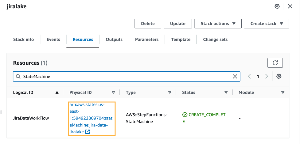
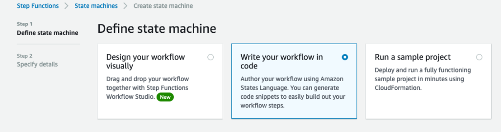
- On the Step Functions console, create a new state machine.
- Select Write your workflow in code.

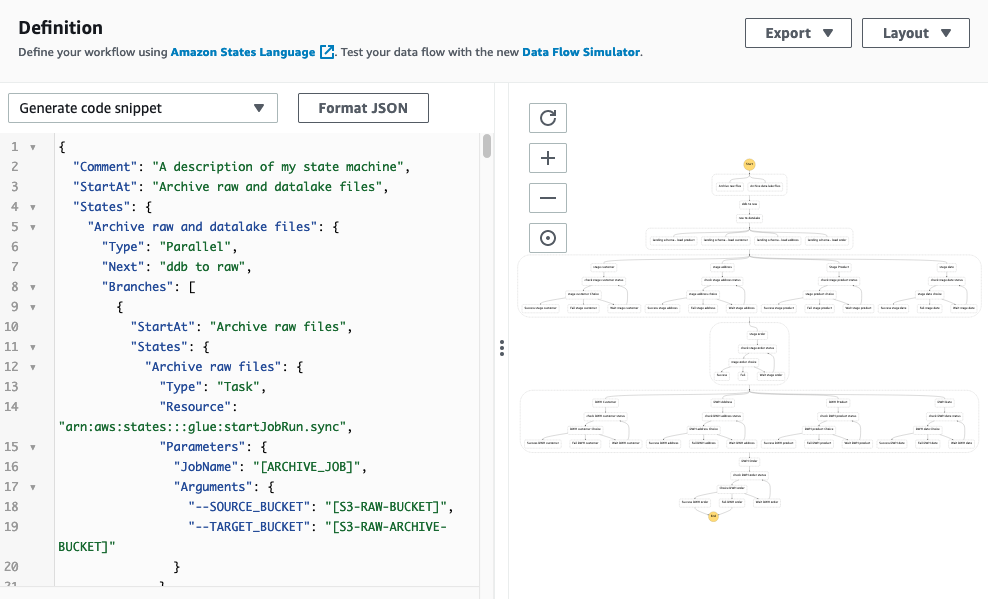
- Enter the stepfunction_workflow.json code into the definition, replacing all placeholders with the appropriate values:
- [REDSHIFT-CLUSTER-IDENTIFIER] – Use the value for
ClusterName (from the Outputs tab in the CloudFormation stack).
- [REDSHIFT-DATABASE] – Use the value for
salesdwh (unless changed, this is the default database in the CloudFormation template).
We use the Step Functions IAM role from the CloudFormation template.

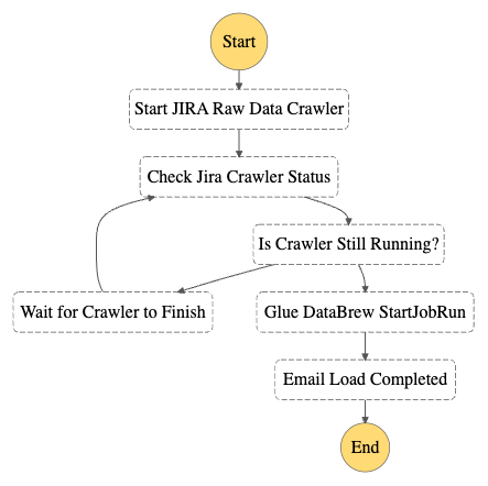
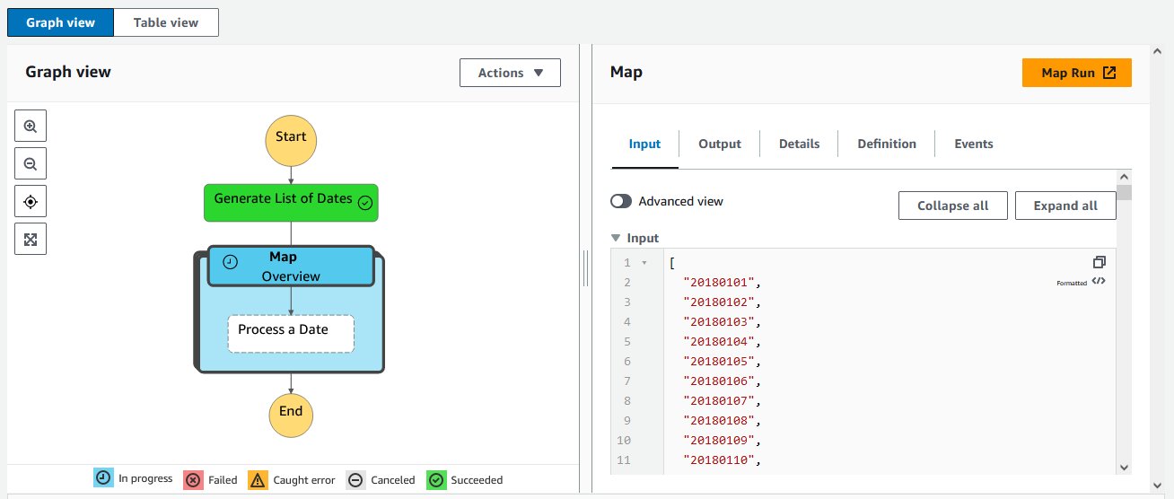
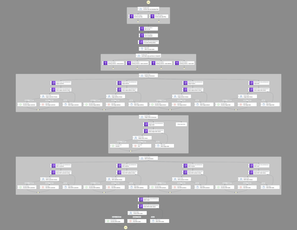
This JSON code generates the following pipeline.

Starting from the top, the workflow contains the following steps:
- We archive any existing raw and data lake files.
- We add two AWS Glue
StartJobRun tasks that run sequentially: first to export the data from DynamoDB to our raw bucket, then from the raw bucket to our data lake.
- After that, we parallelize the landing of data from Amazon S3 to Amazon Redshift.
- We transform and load the data into our data warehouse using the Amazon Redshift Data API. Because this is asynchronous, we need to check the status of the runs before moving down the pipeline.
- After we move the data load from landing to staging, we truncate the landing tables.
- We load the dimensions of our target data warehouse (
dwh) first, and finally we load our single fact table with its foreign key dependency on the preceding dimension tables.
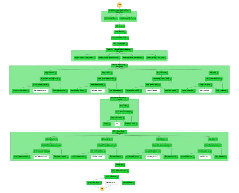
The following figure illustrates a successful run.

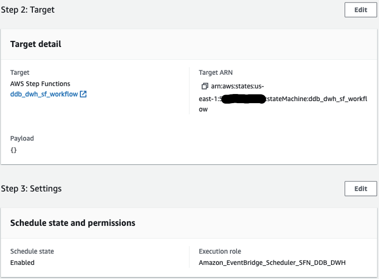
After we set up the workflow, we can use EventBridge to schedule a daily midnight run, where the target is a Step Functions StartExecution API calling our state machine. Under the workflow permissions, choose Create a new role for this schedule and optionally rename it.


Query the data warehouse
We can verify the data has been successfully loaded into Amazon Redshift with a query.

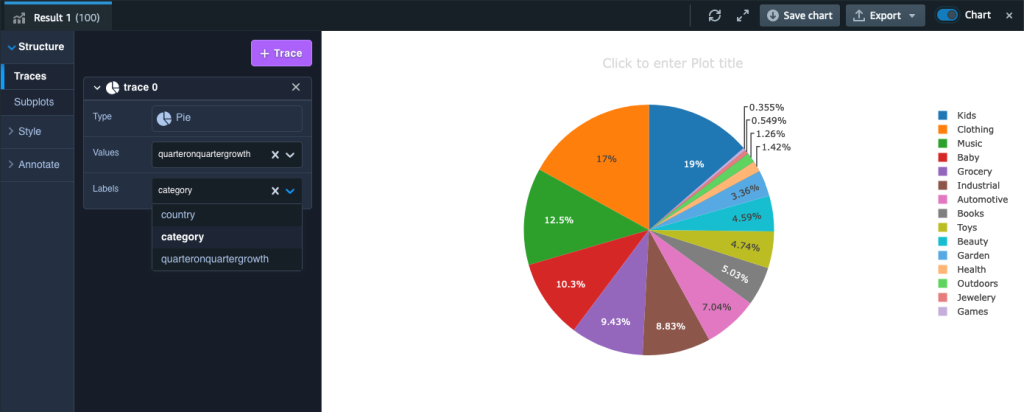
After we have the data loaded into Amazon Redshift, we’re ready to answer the query asked at the start of this post: what is the year-on-year quarterly sales growth by product and country? The query looks like the following code (depending on your dataset, you may need to select alternative years and quarters):
with sales2021q2
as
(
  select d.year, d.quarter,a.country,p.category,sum(o.price) as revenue2021q2
  from dwh.order o
  join dwh.date d on o.datekey=d.datekey
  join dwh.product p on o.productkey=p.productkey
  join dwh.address a on a.addresskey=o.addresskey
  where d.year=2021 and d.quarter=2
  group by d.year, d.quarter,a.country,p.category
  ),
sales2022q2
as
(
  select d.year, d.quarter,a.country,p.category,sum(o.price) as revenue2022q2
  from dwh.order o
  join dwh.date d on o.datekey=d.datekey
  join dwh.product p on o.productkey=p.productkey
  join dwh.address a on a.addresskey=o.addresskey
  where d.year=2022 and d.quarter=2
  group by d.year, d.quarter,a.country,p.category
  )

select a.country,a.category, ((revenue2022q2 - revenue2021q2)/revenue2021q2)*100 as quarteronquartergrowth
from sales2022q2 a
join sales2021q2 b on a.country=b.country and a.category=b.category
order by a.country,a.category
We can visualize the results in Amazon Redshift Query Editor V2 by toggling the chart option and setting Type as Pie, Values as quarteronquartergrowth, and Labels as category.

Cost considerations
We give a brief outline of the indicative costs associated with the key services covered in our solution based on us-east-1 Region pricing using the AWS Pricing Calculator:
- DynamoDB – With on-demand settings for 1.5 million items (average size of 355 bytes) and associated write and read capacity plus PITR storage, the cost of DynamoDB is approximately $2 per month.
- AWS Glue DynamoDB export connector – This connector utilizes the DynamoDB export to Amazon S3 feature. This has no hourly cost—you only pay for the gigabytes of data exported to Amazon S3 ($0.11 per GiB).
- Amazon S3 – You pay for storing objects in your S3 buckets. The rate you’re charged depends on your objects’ size, how long you stored the objects during the month, and the storage class. In our solution, we used S3 Standard for our data lake and S3 Standard – Infrequent Access for archive. Standard-IA storage is $0.0125 per GB/month; Standard storage is $0.023 per GB/month.
- AWS Glue Jobs – With AWS Glue, you only pay for the time your ETL job takes to run. There are no resources to manage, no upfront costs, and you are not charged for startup or shutdown time. AWS charges you an hourly rate based on the number of Data Processing Units (DPUs) used to run your ETL job. A single DPU provides 4 vCPU and 16 GB of memory. Every one of our nine Spark jobs uses 10 DPUs and has an average runtime of 3 minutes. This gives an approximate cost of $0.29 per job.
- Amazon Redshift – We provisioned two RA3.4xlarge nodes for our Amazon Redshift cluster. If run on-demand, each node costs $3.26 per hour. If utilized 24/7, our monthly cost would be approximately $4,759.60. You should evaluate your workload to determine what cost savings can be achieved by using Amazon Redshift Serverless or using Amazon Redshift provisioned reserved instances.
- Step Functions – You are charged based on the number of state transitions required to run your application. Step Functions counts a state transition as each time a step of your workflow is run. You’re charged for the total number of state transitions across all your state machines, including retries. The Step Functions free tier includes 4,000 free state transitions per month. Thereafter, it’s $0.025 per 1,000 state transitions.
Clean up
Remember to delete any resources created through the CloudFormation stack. You first need to manually empty and delete the S3 buckets. Then you can delete the CloudFormation stack using the AWS CloudFormation console or AWS Command Line Interface (AWS CLI). For instructions, refer to Clean up your “hello, world!” application and related resources.
Summary
In this post, we demonstrated how you can export data from DynamoDB to Amazon S3 and Amazon Redshift to perform advanced analytics. We built an automated data pipeline that you can use to perform a batch ELT process that can be scheduled to run daily, weekly, or monthly and can scale to handle very large workloads.
Please leave your feedback or comments in the comments section.
About the Author

Altaf Hussain is an Analytics Specialist Solutions Architect at AWS. He helps customers around the globe design and optimize their big data and data warehousing solutions.
Appendix
To extract the data from DynamoDB and load it into our Amazon Redshift database, we can use the Spark script editor and upload the files from GlueSparkJobs.zip to create each individual job necessary to perform the extract and load. If you choose to do this, remember to update, where appropriate, the account ID and Region placeholders in the scripts. Also, on the Job details tab under Advanced properties, add the Amazon Redshift connection.


 Aarthi Srinivasan is a Senior Big Data Architect with AWS Lake Formation. She likes building data lake solutions for AWS customers and partners. When not on the keyboard, she explores the latest science and technology trends and spends time with her family.


 Raj Ramasubbu is a Sr. Analytics Specialist Solutions Architect focused on big data and analytics and AI/ML with Amazon Web Services. He helps customers architect and build highly scalable, performant, and secure cloud-based solutions on AWS. Raj provided technical expertise and leadership in building data engineering, big data analytics, business intelligence, and data science solutions for over 18 years prior to joining AWS. He helped customers in various industry verticals like healthcare, medical devices, life science, retail, asset management, car insurance, residential REIT, agriculture, title insurance, supply chain, document management, and real estate.
 Rahul Sonawane is a Principal Analytics Solutions Architect at AWS with AI/ML and Analytics as his area of specialty.
 Sundeep Kumar is a Sr. Data Architect, Data Lake at AWS, helping customers build data lake and analytics platform and solutions. When not building and designing data lakes, Sundeep enjoys listening music and playing guitar.
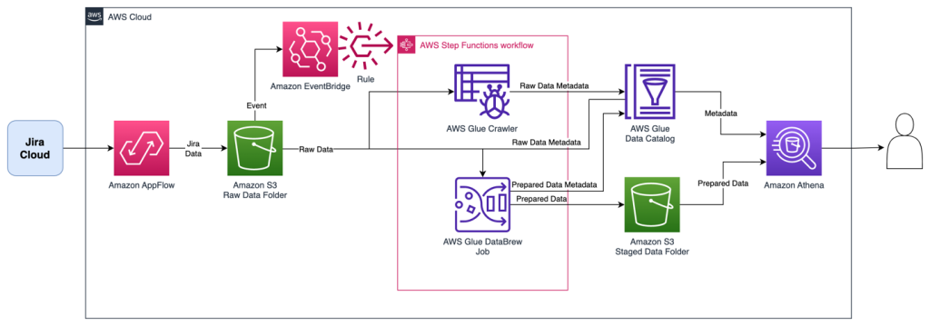


 Tom Romano is a Sr. Solutions Architect for AWS World Wide Public Sector from Tampa, FL, and assists GovTech and EdTech customers as they create new solutions that are cloud native, event driven, and serverless. He is an enthusiastic Python programmer for both application development and data analytics, and is an Analytics Specialist. In his free time, Tom flies remote control model airplanes and enjoys vacationing with his family around Florida and the Caribbean.
 Shane Thompson is a Sr. Solutions Architect based out of San Luis Obispo, California, working with AWS Startups. He works with customers who use AI/ML in their business model and is passionate about democratizing AI/ML so that all customers can benefit from it. In his free time, Shane loves to spend time with his family and travel around the world.


 Mitesh Patel is a Principal Solutions Architect at AWS with specialization in data analytics and machine learning. He is passionate about helping customers building scalable, secure and cost effective cloud native solutions in AWS to drive the business growth. He lives in DC Metro area with his wife and two kids.
 Sumitha AP is a Sr. Solutions Architect at AWS. She works with customers and help them attain their business objectives by designing secure, scalable, reliable, and cost-effective solutions in the AWS Cloud. She has a focus on data and analytics and provides guidance on building analytics solutions on AWS.
 Deepti Venuturumilli is a Sr. Solutions Architect in AWS. She works with commercial segment customers and AWS partners to accelerate customers’ business outcomes by providing expertise in AWS services and modernize their workloads. She focuses on data analytics workloads and setting up modern data strategy on AWS.
 Deepthi Paruchuri is an AWS Solutions Architect based in NYC. She works closely with customers to build cloud adoption strategy and solve their business needs by designing secure, scalable, and cost-effective solutions in the AWS cloud.


 Rohit Vashishtha is a Senior Analytics Specialist Solutions Architect at AWS based in Dallas, Texas. He has 17 years of experience architecting, building, leading, and maintaining big data platforms. Rohit helps customers modernize their analytic workloads using the breadth of AWS services and ensures that customers get the best price/performance with utmost security and data governance.


 Mikhail Smirnov is a Sr. Software Dev Engineer on the AWS Glue team and part of the AWS Glue DataBrew development team. Outside of work, his interests include learning to play guitar and traveling with his family.
 Gonzalo Herreros is a Sr. Big Data Architect on the AWS Glue team. Based on Dublin, Ireland, he helps customers succeed with big data solutions based on AWS Glue. On his spare time, he enjoys board games and cycling.


 Noritaka Sekiyama is a Principal Big Data Architect on the AWS Glue team. He works based in Tokyo, Japan. He is responsible for building software artifacts to help customers. In his spare time, he enjoys cycling with his road bike.

 Noritaka Sekiyama is a Principal Big Data Architect on the AWS Glue team. He works based in Tokyo, Japan. He is responsible for building software artifacts to help customers. In his spare time, he enjoys cycling with his road bike.
 Gal Heyne is a Product Manager for AWS Glue with a strong focus on AI/ML, data engineering, and BI, and is based in California. She is passionate about developing a deep understanding of customers’ business needs and collaborating with engineers to design easy-to-use data products. In her spare time, she enjoys playing card games.


 Qiushuang Feng is a Solutions Architect at AWS, responsible for Enterprise customers’ technical architecture design, consulting, and design optimization on AWS Cloud services. Before joining AWS, Qiushuang worked in IT companies such as IBM and Oracle, and accumulated rich practical experience in development and analytics.
 Greg Huang is a Senior Solutions Architect at AWS with expertise in technical architecture design and consulting for the China G1000 team. He is dedicated to deploying and utilizing enterprise-level applications on AWS Cloud services. He possesses nearly 20 years of rich experience in large-scale enterprise application development and implementation, having worked in the cloud computing field for many years. He has extensive experience in helping various types of enterprises migrate to the cloud. Prior to joining AWS, he worked for well-known IT enterprises such as Baidu and Oracle.
 Maciej Torbus is a Principal Customer Solutions Manager within Strategic Accounts at Amazon Web Services. With extensive experience in large-scale migrations, he focuses on helping customers move their applications and systems to highly reliable and scalable architectures in AWS. Outside of work, he enjoys sailing, traveling, and restoring vintage mechanical watches.

 Jacques Steyn runs the Altron Data Analytics Professional Services. He has been leading the building of data warehouses and analytic solutions for the past 20 years. In his free time, he spends time with his family, whether it be on the golf , walking in the mountains, or camping in South Africa, Botswana, and Namibia.
 Jason Yung is a Principal Analytics Specialist with Amazon Web Services. Working with Senior Executives across the Europe and Asia-Pacific Regions, he helps customers become data-driven by understanding their use cases and articulating business value through Amazon mechanisms. In his free time, he spends time looking after a very active 1-year-old daughter, alongside juggling geeky activities with respectable hobbies such as cooking sub-par food.
 Michele Lamarca is a Senior Solutions Architect with Amazon Web Services. He helps architect and run Solutions Accelerators in Europe to enable customers to become hands-on with AWS services and build prototypes quickly to release the value of data in the organization. In his free time, he reads books and tries (hopelessly) to improve his jazz piano skills.
 Hamza is a Specialist Solutions Architect with Amazon Web Services. He runs Solutions Accelerators in EMEA regions to help customers accelerate their journey to move from an idea into a solution in production. In his free time, he spends time with his family, meets with friends, swims in the municipal swimming pool, and learns new skills.
 AWS Global Summits – Check your calendars and sign up for the AWS Summit close to where you live or work:


 Nishchai JM is an Analytics Specialist Solutions Architect at Amazon Web services. He specializes in building Big-data applications and help customer to modernize their applications on Cloud. He thinks Data is new oil and spends most of his time in deriving insights out of the Data.
 Varad Ram is Senior Solutions Architect in Amazon Web Services. He likes to help customers adopt to cloud technologies and is particularly interested in artificial intelligence. He believes deep learning will power future technology growth. In his spare time, he like to be outdoor with his daughter and son.
 Narendra Gupta is a Specialist Solutions Architect at AWS, helping customers on their cloud journey with a focus on AWS analytics services. Outside of work, Narendra enjoys learning new technologies, watching movies, and visiting new places
 Arun A K is a Big Data Solutions Architect with AWS. He works with customers to provide architectural guidance for running analytics solutions on the cloud. In his free time, Arun loves to enjoy quality time with his family
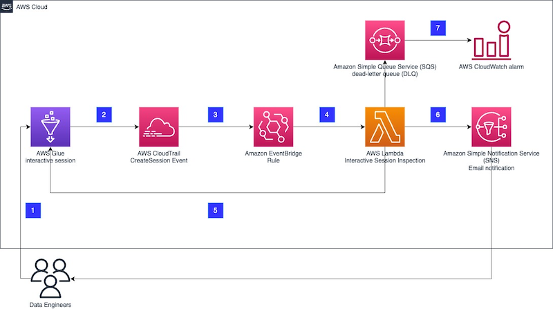
 Nicolas Jacob Baer is a Senior Cloud Application Architect with a strong focus on data engineering and machine learning, based in Switzerland. He works closely with enterprise customers to design data platforms and build advanced analytics/ml use-cases.
 Luca Mazzaferro is a Senior DevOps Architect at Amazon Web Services. He likes to have infrastructure automated, reproducible and secured. In his free time he likes to cook, especially pizza.
 Kemeng Zhang is a Cloud Application Architect with a strong focus on machine learning and UX, based in Switzerland. She works closely with customers to design user experiences and build advanced analytics/ml use-cases.
 Mark Walser, a Senior Global Data Architect at Amazon Web Services, collaborates with customers to develop innovative Big Data solutions that solve business problems and speed up the adoption of AWS services. Outside of work, he finds pleasure in running, swimming, and all things related to technology.


 Anderson Santos is a Senior Solutions Architect at Amazon Web Services. He works with AWS Enterprise customers to provide guidance and technical assistance, helping them improve the value of their solutions when using AWS.
 Arun Pradeep Selvaraj is a Senior Solutions Architect and is part of Analytics TFC at AWS. Arun is passionate about working with his customers and stakeholders on digital transformations and innovation in the cloud while continuing to learn, build and reinvent. He is creative, fast-paced, deeply customer-obsessed and leverages the working backwards process to build modern architectures to help customers solve their unique challenges.
 Patrick Muller is a Senior Solutions Architect and a valued member of the Datalab. With over 20 years of expertise in analytics, data warehousing, and distributed systems, he brings extensive knowledge to the table. Patrick’s passion lies in evaluating new technologies and assisting customers with innovative solutions. During his free time, he enjoys watching soccer.
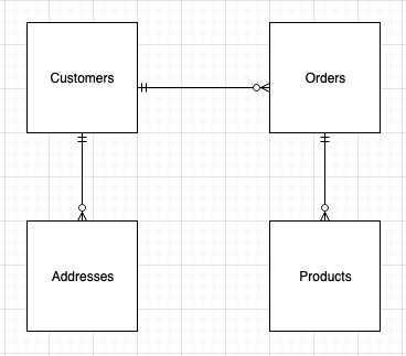


 Srividya Parthasarathy is a Senior Big Data Architect on the AWS Lake Formation team. She enjoys building data mesh solutions and sharing them with the community.
 Sandeep Adwankar is a Senior Technical Product Manager at AWS. Based in the California Bay Area, he works with customers around the globe to translate business and technical requirements into products that enable customers to improve how they manage, secure, and access data.