Amazon Managed Workflows for Apache Airflow (Amazon MWAA) is a managed orchestration service for Apache Airflow that significantly improves security and availability, and reduces infrastructure management overhead when setting up and operating end-to-end data pipelines in the cloud.
Today, we are announcing the availability of Apache Airflow version 2.9.2 environments on Amazon MWAA. Apache Airflow 2.9.2 introduces several notable enhancements, such as new API endpoints for improved dataset management, advanced scheduling options including conditional expressions for dataset dependencies, the combination of dataset and time-based schedules, and custom names in dynamic task mapping for better readability of your DAGs.
In this post, we walk you through some of these new features and capabilities, how you can use them, and how you can set up or upgrade your Amazon MWAA environments to Airflow 2.9.2.
With each new version release, the Apache Airflow community is innovating to make Airflow more data-aware, enabling you to build reactive, event-driven workflows that can accommodate changes in datasets, either between Airflow environments or in external systems. Let’s go through some of these new capabilities.
Logical operators and conditional expressions for DAG scheduling
Prior to the introduction of this capability, users faced significant limitations when working with complex scheduling scenarios involving multiple datasets. Airflow’s scheduling capabilities were restricted to logical AND combinations of datasets, meaning that a DAG run would only be created after all specified datasets were updated since the last run. This rigid approach posed challenges for workflows that required more nuanced triggering conditions, such as running a DAG when any one of several datasets was updated or when specific combinations of dataset updates occurred.
With the release of Airflow 2.9.2, you can now use logical operators (AND and OR) and conditional expressions to define intricate scheduling conditions based on dataset updates. This feature allows for granular control over workflow triggers, enabling DAGs to be scheduled whenever a specific dataset or combination of datasets is updated.
For example, in the financial services industry, a risk management process might need to be run whenever trading data from any regional market is refreshed, or when both trading and regulatory updates are available. The new scheduling capabilities available in Amazon MWAA allow you to express such complex logic using simple expressions. The following diagram illustrates the dependency we need to establish.
The following DAG code contains the logical operations to implement these dependencies:
With Airflow 2.9.2 environments, Amazon MWAA now has a more comprehensive scheduling mechanism that combines the flexibility of data-driven execution with the consistency of time-based schedules.
Consider a scenario where your team is responsible for managing a data pipeline that generates daily sales reports. This pipeline relies on data from multiple sources. Although it’s essential to generate these sales reports on a daily basis to provide timely insights to business stakeholders, you also need to make sure the reports are up to date and reflect important data changes as soon as possible. For instance, if there’s a significant influx of orders during a promotional campaign, or if inventory levels change unexpectedly, the report should incorporate these updates to maintain relevance.
Relying solely on time-based scheduling for this type of data pipeline could lead to potential issues such as outdated information and infrastructure resource wastage.
The DatasetOrTimeSchedule feature introduced in Airflow 2.9 adds the capability to combine conditional dataset expressions with time-based schedules. This means that your workflow can be invoked not only at predefined intervals but also whenever there are updates to the specified datasets, with the specific dependency relationship among them. The following diagram illustrates how you can use this capability to accommodate such scenarios.
See the following DAG code for an example implementation:
from airflow.decorators import dag, task
from airflow.timetables.datasets import DatasetOrTimeSchedule
from airflow.timetables.trigger import CronTriggerTimetable
from airflow.datasets import Dataset
from datetime import datetime

# Define datasets
orders_dataset = Dataset("s3://path/to/orders/data")
inventory_dataset = Dataset("s3://path/to/inventory/data")
customer_dataset = Dataset("s3://path/to/customer/data")

# Combine datasets using logical operators
combined_dataset = (orders_dataset & inventory_dataset) | customer_dataset

@dag(
    dag_id="dataset_time_scheduling",
    start_date=datetime(2024, 1, 1),
    schedule=DatasetOrTimeSchedule(
        timetable=CronTriggerTimetable("0 0 * * *", timezone="UTC"),  # Daily at midnight
        datasets=combined_dataset
    ),
    catchup=False,
)
def dataset_time_scheduling_pipeline():
    @task
    def process_orders():
        # Task logic for processing orders
        pass

    @task
    def update_inventory():
        # Task logic for updating inventory
        pass

    @task
    def update_customer_data():
        # Task logic for updating customer data
        pass

    orders_task = process_orders()
    inventory_task = update_inventory()
    customer_task = update_customer_data()

dataset_time_scheduling_pipeline()
In the example, the DAG will be run under two conditions:
When the time-based schedule is met (daily at midnight UTC)
When the combined dataset condition is met, when there are updates to both orders and inventory data, or when there are updates to customer data, regardless of the other datasets
This flexibility enables you to create sophisticated scheduling rules that cater to the unique requirements of your data pipelines, so they run when necessary and incorporate the latest data updates from multiple sources.
For more details on data-aware scheduling, refer to Data-aware scheduling in the Airflow documentation.
Dataset event REST API endpoints
Prior to the introduction of this feature, making your Airflow environment aware of changes to datasets in external systems was a challenge—there was no option to mark a dataset as externally updated. With the new dataset event endpoints feature, you can programmatically initiate dataset-related events. The REST API has endpoints to create, list, and delete dataset events.
This capability enables external systems and applications to seamlessly integrate and interact with your Amazon MWAA environment. It significantly improves your ability to expand your data pipeline’s capacity for dynamic data management.
As an example, running the following code from an external system allows you to invoke a dataset event in the target Amazon MWAA environment. This event could then be handled by downstream processes or workflows, enabling greater connectivity and responsiveness in data-driven workflows that rely on timely data updates and interactions.
Airflow 2.9.2 also includes features to ease the operation and monitoring of your environments. Let’s explore some of these new capabilities.
Dag auto-pausing
Customers are using Amazon MWAA to build complex data pipelines with multiple interconnected tasks and dependencies. When one of these pipelines encounters an issue or failure, it can result in a cascade of unnecessary and redundant task runs, leading to wasted resources. This problem is particularly prevalent in scenarios where pipelines run at frequent intervals, such as hourly or daily. A common scenario is a critical pipeline that starts failing during the evening, and due to the failure, it continues to run and fails repeatedly until someone manually intervenes the next morning. This can result in dozens of unnecessary tasks, consuming valuable compute resources and potentially causing data corruption or inconsistencies.
The DAG auto-pausing feature aims to address this challenge by introducing two new configuration parameters:
max_consecutive_failed_dag_runs_per_dag – This is a global Airflow configuration setting. It allows you to specify the maximum number of consecutive failed DAG runs before the DAG is automatically paused.
max_consecutive_failed_dag_runs – This is a DAG-level argument. It overrides the previous global configuration, allowing you to set a custom threshold for each DAG.
In the following code example, we define a DAG with a single PythonOperator. The failing_task is designed to fail by raising a ValueError. The key configuration for DAG auto-pausing is the max_consecutive_failed_dag_runs parameter set in the DAG object. By setting max_consecutive_failed_dag_runs=3, we’re instructing Airflow to automatically pause the DAG after it fails three consecutive times.
from airflow.decorators import dag, task
from datetime import datetime, timedelta

@task
def failing_task():
    raise ValueError("This task is designed to fail")

@dag(
    dag_id="auto_pause",
    start_date=datetime(2023, 1, 1),
    schedule_interval=timedelta(minutes=1),  # Run every minute
    catchup=False,
    max_consecutive_failed_dag_runs=3,  # Set the maximum number of consecutive failed DAG runs
)
def example_dag_with_auto_pause():
    failing_task_instance = failing_task()

example_dag_with_auto_pause()
With this parameter, you can now configure your Airflow DAGs to automatically pause after a specified number of consecutive failures.
To learn more, refer to DAG Auto-pausing in the Airflow documentation.
CLI support for bulk pause and resume of DAGs
As the number of DAGs in your environment grows, managing them becomes increasingly challenging. Whether for upgrading or migrating environments, or other operational activities, you may need to pause or resume multiple DAGs. This process can become a daunting cyclical endeavor because you need to navigate through the Airflow UI, manually pausing or resuming DAGs one at a time. These manual activities are time consuming and increase the risk of human error that can result in missteps and lead to data inconsistencies or pipeline disruptions. The previous CLI commands for pausing and resuming DAGs could only handle one DAG at a time, making it inefficient.
Airflow 2.9.2 improves these CLI commands by adding the capability to treat DAG IDs as regular expressions, allowing you to pause or resume multiple DAGs with a single command. This new feature eliminates the need for repetitive manual intervention or individual DAG operations, significantly reducing the risk of human error, providing reliability and consistency in your data pipelines.
As an example, to pause all DAGs generating daily liquidity reporting using Amazon Redshift as a data source, you can use the following CLI command with a regular expression:
Dynamic Task Mapping was added in Airflow 2.3. This powerful feature allows workflows to create tasks dynamically at runtime based on data. Instead of relying on the DAG author to predict the number of tasks needed in advance, the scheduler can generate the appropriate number of copies of a task based on the output of a previous task. Of course, with great powers comes great responsibilities. By default, dynamically mapped tasks were assigned numeric indexes as names. In complex workflows involving high numbers of mapped tasks, it becomes increasingly challenging to pinpoint the specific tasks that require attention, leading to potential delays and inefficiencies in managing and maintaining your data workflows.
Airflow 2.9 introduces the map_index_template parameter, a highly requested feature that addresses the challenge of task identification in Dynamic Task Mapping. With this capability, you can now provide custom names for your dynamically mapped tasks, enhancing visibility and manageability within the Airflow UI.
See the following example:
from airflow.decorators import dag
from airflow.operators.python import PythonOperator
from datetime import datetime, timedelta

def process_data(data):
    # Perform data processing logic here
    print(f"Processing data: {data}")

@dag(
    dag_id="custom_task_mapping_example",
    start_date=datetime(2023, 1, 1),
    schedule_interval=None,
    catchup=False,
)
def custom_task_mapping_example():
    mapped_processes = PythonOperator.partial(
        task_id="process_data_source",
        python_callable=process_data,
        map_index_template="Processing source={{ task.op_args[0] }}",
    ).expand(op_args=[["source_a"], ["source_b"], ["source_c"]])

custom_task_mapping_example()
The key aspect in the code is the map_index_template parameter specified in the PythonOperator.partial call. This Jinja template instructs Airflow to use the values of the ops_args environment variable as the map index for each dynamically mapped task instance. In the Airflow UI, you will see three task instances with the indexes source_a, source_b, and source_c, making it straightforward to identify and track the tasks associated with each data source. In case of failures, this capability improves monitoring and troubleshooting.
The map_index_template feature goes beyond simple template rendering, offering dynamic injection capabilities into the rendering context. This functionality unlocks greater levels of flexibility and customization when naming dynamically mapped tasks.
Refer to Named mapping in the Airflow documentation to learn more about named mapping.
TaskFlow decorator for Bash commands
Writing complex Bash commands and scripts using the traditional Airflow BashOperator may bring challenges in areas such as code consistency, task dependencies definition, and dynamic command generation. The new @task.bash decorator addresses these challenges, allowing you to define Bash statements using Python functions, making the code more readable and maintainable. It seamlessly integrates with Airflow’s TaskFlow API, enabling you to define dependencies between tasks and create complex workflows. You can also use Airflow’s scheduling and monitoring capabilities while maintaining a consistent coding style.
The following sample code showcases how the @task.bash decorator simplifies the integration of Bash commands into DAGs, while using the full capabilities of Python for dynamic command generation and data processing:
from airflow.decorators import dag, task
from datetime import datetime, timedelta

default_args = {
    'owner': 'airflow',
    'retries': 1,
    'retry_delay': timedelta(minutes=5),
}

# Sample customer data
customer_data = """
id,name,age,city
1,John Doe,35,New York
2,Jane Smith,42,Los Angeles
3,Michael Johnson,28,Chicago
4,Emily Williams,31,Houston
5,David Brown,47,Phoenix
"""

# Sample order data
order_data = """
order_id,customer_id,product,quantity,price
101,1,Product A,2,19.99
102,2,Product B,1,29.99
103,3,Product A,3,19.99
104,4,Product C,2,14.99
105,5,Product B,1,29.99
"""

@dag(
    dag_id='task-bash-customer_order_analysis',
    default_args=default_args,
    start_date=datetime(2023, 1, 1),
    schedule_interval=timedelta(days=1),
    catchup=False,
)
def customer_order_analysis_dag():
    @task.bash
    def clean_data():
        # Clean customer data
        customer_cleaning_commands = """
            echo '{}' > cleaned_customers.csv
            cat cleaned_customers.csv | sed 's/,/;/g' > cleaned_customers.csv
            cat cleaned_customers.csv | awk 'NR > 1' > cleaned_customers.csv
        """.format(customer_data)

        # Clean order data
        order_cleaning_commands = """
            echo '{}' > cleaned_orders.csv
            cat cleaned_orders.csv | sed 's/,/;/g' > cleaned_orders.csv
            cat cleaned_orders.csv | awk 'NR > 1' > cleaned_orders.csv
        """.format(order_data)

        return customer_cleaning_commands + "\n" + order_cleaning_commands

    @task.bash
    def transform_data(cleaned_customers, cleaned_orders):
        # Transform customer data
        customer_transform_commands = """
            cat {cleaned_customers} | awk -F';' '{{printf "%s,%s,%s\\n", $1, $2, $3}}' > transformed_customers.csv
        """.format(cleaned_customers=cleaned_customers)

        # Transform order data
        order_transform_commands = """
            cat {cleaned_orders} | awk -F';' '{{printf "%s,%s,%s,%s,%s\\n", $1, $2, $3, $4, $5}}' > transformed_orders.csv
        """.format(cleaned_orders=cleaned_orders)

        return customer_transform_commands + "\n" + order_transform_commands

    @task.bash
    def analyze_data(transformed_customers, transformed_orders):
        analysis_commands = """
            # Calculate total revenue
            total_revenue=$(awk -F',' '{{sum += $5 * $4}} END {{printf "%.2f", sum}}' {transformed_orders})
            echo "Total revenue: $total_revenue"

            # Find customers with multiple orders
            customers_with_multiple_orders=$(
                awk -F',' '{{orders[$2]++}} END {{for (c in orders) if (orders[c] > 1) printf "%s,", c}}' {transformed_orders}
            )
            echo "Customers with multiple orders: $customers_with_multiple_orders"

            # Find most popular product
            popular_product=$(
                awk -F',' '{{products[$3]++}} END {{max=0; for (p in products) if (products[p] > max) {{max=products[p]; popular=p}}}} END {{print popular}}'
            {transformed_orders})
            echo "Most popular product: $popular_product"
        """.format(transformed_customers=transformed_customers, transformed_orders=transformed_orders)

        return analysis_commands

    cleaned_data = clean_data()
    transformed_data = transform_data(cleaned_data, cleaned_data)
    analysis_results = analyze_data(transformed_data, transformed_data)

customer_order_analysis_dag()
Upon successful creation of an Airflow 2.9 environment in Amazon MWAA, certain packages are automatically installed on the scheduler and worker nodes. For a complete list of installed packages and their versions, refer to Apache Airflow provider packages installed on Amazon MWAA environments. You can install additional packages using a requirements file.
Upgrade from older versions of Airflow to version 2.9.2
In this post, we announced the availability of Apache Airflow 2.9 environments in Amazon MWAA. We discussed how some of the latest features added in the release enable you to design more reactive, event-driven workflows, such as DAG scheduling based on the result of logical operations, and the availability of endpoints in the REST API to programmatically create dataset events. We also provided some sample code to show the implementation in Amazon MWAA.
Apache, Apache Airflow, and Airflow are either registered trademarks or trademarks of the Apache Software Foundation in the United States and/or other countries.
About the authors
Hernan Garcia is a Senior Solutions Architect at AWS, based out of Amsterdam, working with enterprises in the Financial Services Industry. He specializes in application modernization and supports customers in the adoption of serverless technologies.
Parnab Basak is a Solutions Architect and a Serverless Specialist at AWS. He specializes in creating new solutions that are cloud native using modern software development practices like serverless, DevOps, and analytics. Parnab works closely in the analytics and integration services space helping customers adopt AWS services for their workflow orchestration needs.
In this post, we continue with our recommendations for achieving least privilege at scale with AWS Identity and Access Management (IAM). In Part 1 of this two-part series, we described the first five of nine strategies for implementing least privilege in IAM at scale. We also looked at a few mental models that can assist you to scale your approach. In this post, Part 2, we’ll continue to look at the remaining four strategies and related mental models for scaling least privilege across your organization.
6. Empower developers to author application policies
If you’re the only developer working in your cloud environment, then you naturally write your own IAM policies. However, a common trend we’ve seen within organizations that are scaling up their cloud usage is that a centralized security, identity, or cloud team administrator will step in to help developers write customized IAM policies on behalf of the development teams. This may be due to variety of reasons, including unfamiliarity with the policy language or a fear of creating potential security risk by granting excess privileges. Centralized creation of IAM policies might work well for a while, but as the team or business grows, this practice often becomes a bottleneck, as indicated in Figure 1.
Figure 1: Bottleneck in a centralized policy authoring process
This mental model is known as the theory of constraints. With this model in mind, you should be keen to search for constraints, or bottlenecks, faced by your team or organization, identify the root cause, and solve for the constraint. That might sound obvious, but when you’re moving at a fast pace, the constraint might not appear until agility is already impaired. As your organization grows, a process that worked years ago might no longer be effective today.
A software developer generally understands the intent of the applications they build, and to some extent the permissions required. At the same time, the centralized cloud, identity, or security teams tend to feel they are the experts at safely authoring policies, but lack a deep knowledge of the application’s code. The goal here is to enable developers to write the policies in order to mitigate bottlenecks.
The question is, how do you equip developers with the right tools and skills to confidently and safely create the required policies for their applications? A simple way to start is by investing in training. AWS offers a variety of formal training options and ramp-up guides that can help your team gain a deeper understanding of AWS services, including IAM. However, even self-hosting a small hackathon or workshop session in your organization can drive improved outcomes. Consider the following four workshops as simple options for self-hosting a learning series with your teams.
IAM policy learning experience workshop – Learn how to write different types of IAM policies and implement access controls on principals and resources, using conditions to scope down access.
IAM troubleshooting workshop – Learn how to create fine-grained access policies with the help of the IAM API, AWS Management Console, IAM Access Analyzer, and AWS CloudTrail, and review key concepts of the IAM policy evaluation logic.
Refining IAM Permissions Like A Pro – Learn how to use IAM Access Analyzer programmatically, use tools to check IAM policies in CI/CD pipeline and AWS Lambda functions, and get hands-on practice in using the tools from the perspectives of both Security and DevOps teams.
As a next step, you can help your teams along the way by setting up processes that foster collaboration and improve quality. For example, peer reviews are highly recommended, and we’ll cover this later. Additionally, administrators can use AWS native tools such as permissions boundaries and IAM Access Analyzer policy generation to help your developers begin to author their own policies more safely.
Let’s look at permissions boundaries first. An IAM permissions boundary should generally be used to delegate the responsibility of policy creation to your development team. You can set up the developer’s IAM role so that they can create new roles only if the new role has a specific permissions boundary attached to it, and that permissions boundary allows you (as an administrator) to set the maximum permissions that can be granted by the developer. This restriction is implemented by a condition on the developer’s identity-based policy, requiring that specific actions—such as iam:CreateRole or iam:CreatePolicy—are allowed only if a specified permissions boundary is attached.
In this way, when a developer creates an IAM role or policy to grant an application some set of required permissions, they are required to add the specified permissions boundary that will “bound” the maximum permissions available to that application. So even if the policy that the developer creates—such as for their AWS Lambda function—is not sufficiently fine-grained, the permissions boundary helps the organization’s cloud administrators make sure that the Lambda function’s policy is not greater than a maximum set of predefined permissions. So with permissions boundaries, your development team can be allowed to create new roles and policies (with constraints) without administrators creating a manual bottleneck.
Another tool developers can use is IAM Access Analyzer policy generation. IAM Access Analyzer reviews your CloudTrail logs and autogenerates an IAM policy based on your access activity over a specified time range. This greatly simplifies the process of writing granular IAM policies that allow end users access to AWS services.
A classic use case for IAM Access Analyzer policy generation is to generate an IAM policy within the test environment. This provides a good starting point to help identify the needed permissions and refine your policy for the production environment. For example, IAM Access Analyzer can’t identify the production resources used, so it adds resource placeholders for you to modify and add the specific Amazon Resource Names (ARNs) your application team needs. However, not every policy needs to be customized, and the next strategy will focus on reusing some policies.
7. Maintain well-written policies
Strategies seven and eight focus on processes. The first process we’ll focus on is to maintain well-written policies. To begin, not every policy needs to be a work of art. There is some wisdom in reusing well-written policies across your accounts, because that can be an effective way to scale permissions management. There are three steps to approach this task:
Identify your use cases
Create policy templates
Maintain repositories of policy templates
For example, if you were new to AWS and using a new account, we would recommend that you use AWS managed policies as a reference to get started. However, the permissions in these policies might not fit how you intend to use the cloud as time progresses. Eventually, you would want to identify the repetitive or common use cases in your own accounts and create common policies or templates for those situations.
When creating templates, you must understand who or what the template is for. One thing to note here is that the developer’s needs tend to be different from the application’s needs. When a developer is working with resources in your accounts, they often need to create or delete resources—for example, creating and deleting Amazon Simple Storage Service (Amazon S3) buckets for the application to use.
Conversely, a software application generally needs to read or write data—in this example, to read and write objects to the S3 bucket that was created by the developer. Notice that the developer’s permissions needs (to create the bucket) are different than the application’s needs (reading objects in the bucket). Because these are different access patterns, you’ll need to create different policy templates tailored to the different use cases and entities.
Figure 2 highlights this issue further. Out of the set of all possible AWS services and API actions, there are a set of permissions that are relevant for your developers (or more likely, their DevOps build and delivery tools) and there’s a set of permissions that are relevant for the software applications that they are building. Those two sets may have some overlap, but they are not identical.
Figure 2: Visualizing intersecting sets of permissions by use case
When discussing policy reuse, you’re likely already thinking about common policies in your accounts, such as default federation permissions for team members or automation that runs routine security audits across multiple accounts in your organization. Many of these policies could be considered default policies that are common across your accounts and generally do not vary. Likewise, permissions boundary policies (which we discussed earlier) can have commonality across accounts with low amounts of variation. There’s value in reusing both of these sets of policies. However, reusing policies too broadly could cause challenges if variation is needed—to make a change to a “reusable policy,” you would have to modify every instance of that policy, even if it’s only needed by one application.
You might find that you have relatively common resource policies that multiple teams need (such as an S3 bucket policy), but with slight variations. This is where you might find it useful to create a repeatable template that abides by your organization’s security policies, and make it available for your teams to copy. We call it a template here, because the teams might need to change a few elements, such as the Principals that they authorize to access the resource. The policies for the applications (such as the policy a developer creates to attach to an Amazon Elastic Compute Cloud (Amazon EC2) instance role) are generally more bespoke or customized and might not be appropriate in a template.
Figure 3 illustrates that some policies have low amounts of variation while others are more bespoke.
Figure 3: Identifying bespoke versus common policy types
Regardless of whether you choose to reuse a policy or turn it into a template, an important step is to store these reusable policies and templates securely in a repository (in this case, AWS CodeCommit). Many customers use infrastructure-as-code modules to make it simple for development teams to input their customizations and generate IAM policies that fit their security policies in a programmatic way. Some customers document these policies and templates directly in the repository while others use internal wikis accompanied with other relevant information. You’ll need to decide which process works best for your organization. Whatever mechanism you choose, make it accessible and searchable by your teams.
8. Peer review and validate policies
We mentioned in Part 1 that least privilege is a journey and having a feedback loop is a critical part. You can implement feedback through human review, or you can automate the review and validate the findings. This is equally as important for the core default policies as it is for the customized, bespoke policies.
Let’s start with some automated tools you can use. One great tool that we recommend is using AWS IAM Access Analyzer policy validation and custom policy checks. Policy validation helps you while you’re authoring your policy to set secure and functional policies. The feature is available through APIs and the AWS Management Console. IAM Access Analyzer validates your policy against IAM policy grammar and AWS best practices. You can view policy validation check findings that include security warnings, errors, general warnings, and suggestions for your policy.
Let’s review some of the finding categories.
Finding type
Description
Security
Includes warnings if your policy allows access that AWS considers a security risk because the access is overly permissive.
Errors
Includes errors if your policy includes lines that prevent the policy from functioning.
Warning
Includes warnings if your policy doesn’t conform to best practices, but the issues are not security risks.
Suggestions
Includes suggestions if AWS recommends improvements that don’t impact the permissions of the policy.
Custom policy checks are a new IAM Access Analyzer capability that helps security teams accurately and proactively identify critical permissions in their policies. You can use this to check against a reference policy (that is, determine if an updated policy grants new access compared to an existing version of the policy) or check against a list of IAM actions (that is, verify that specific IAM actions are not allowed by your policy). Custom policy checks use automated reasoning, a form of static analysis, to provide a higher level of security assurance in the cloud.
In Figure 4, you’ll see a typical development workflow. This is a simplified version of a CI/CD pipeline with three stages: a commit stage, a validation stage, and a deploy stage. In the diagram, the developer’s code (including IAM policies) is checked across multiple steps.
Figure 4: A pipeline with a policy validation step
In the commit stage, if your developers are authoring policies, you can quickly incorporate peer reviews at the time they commit to the source code, and this creates some accountability within a team to author least privilege policies. Additionally, you can use automation by introducing IAM Access Analyzer policy validation in a validation stage, so that the work can only proceed if there are no security findings detected. To learn more about how to deploy this architecture in your accounts, see this blog post. For a Terraform version of this process, we encourage you to check out this GitHub repository.
9. Remove excess privileges over time
Our final strategy focuses on existing permissions and how to remove excess privileges over time. You can determine which privileges are excessive by analyzing the data on which permissions are granted and determining what’s used and what’s not used. Even if you’re developing new policies, you might later discover that some permissions that you enabled were unused, and you can remove that access later. This means that you don’t have to be 100% perfect when you create a policy today, but can rather improve your policies over time. To help with this, we’ll quickly review three recommendations:
Restrict unused permissions by using service control policies (SCPs)
Remove unused identities
Remove unused services and actions from policies
First, as discussed in Part 1 of this series, SCPs are a broad guardrail type of control that can deny permissions across your AWS Organizations organization, a set of your AWS accounts, or a single account. You can start by identifying services that are not used by your teams, despite being allowed by these SCPs. You might also want to identify services that your organization doesn’t intend to use. In those cases, you might consider restricting that access, so that you retain access only to the services that are actually required in your accounts. If you’re interested in doing this, we’d recommend that you review the Refining permissions in AWS using last accessed information topic in the IAM documentation to get started.
Second, you can focus your attention more narrowly to identify unused IAM roles, unused access keys for IAM users, and unused passwords for IAM users either at an account-specific level or the organization-wide level. To do this, you can use IAM Access Analyzer’s Unused Access Analyzer capability.
Third, the same Unused Access Analyzer capability also enables you to go a step further to identify permissions that are granted but not actually used, with the goal of removing unused permissions. IAM Access Analyzer creates findings for the unused permissions. If the granted access is required and intentional, then you can archive the finding and create an archive rule to automatically archive similar findings. However, if the granted access is not required, you can modify or remove the policy that grants the unintended access. The following screenshot shows an example of the dashboard for IAM Access Analyzer’s unused access findings.
Figure 5: Screenshot of IAM Access Analyzer dashboard
When we talk to customers, we often hear that the principle of least privilege is great in principle, but they would rather focus on having just enough privilege. One mental model that’s relevant here is the 80/20 rule (also known as the Pareto principle), which states that 80% of your outcome comes from 20% of your input (or effort). The flip side is that the remaining 20% of outcome will require 80% of the effort—which means that there are diminishing returns for additional effort. Figure 6 shows how the Pareto principle relates to the concept of least privilege, on a scale from maximum privilege to perfect least privilege.
Figure 6: Applying the Pareto principle (80/20 rule) to the concept of least privilege
The application of the 80/20 rule to permissions management—such as refining existing permissions—is to identify what your acceptable risk threshold is and to recognize that as you perform additional effort to eliminate that risk, you might produce only diminishing returns. However, in pursuit of least privilege, you’ll still want to work toward that remaining 20%, while being pragmatic about the remainder of the effort.
Remember that least privilege is a journey. Two ways to be pragmatic along this journey are to use feedback loops as you refine your permissions, and to prioritize. For example, focus on what is sensitive to your accounts and your team. Restrict access to production identities first before moving to environments with less risk, such as development or testing. Prioritize reviewing permissions for roles or resources that enable external, cross-account access before moving to the roles that are used in less sensitive areas. Then move on to the next priority for your organization.
Conclusion
Thank you for taking the time to read this two-part series. In these two blog posts, we described nine strategies for implementing least privilege in IAM at scale. Across these nine strategies, we introduced some mental models, tools, and capabilities that can assist you to scale your approach. Let’s consider some of the key takeaways that you can use in your journey of setting, verifying, and refining permissions.
Cloud administrators and developers will then verify permissions. For this task, they can use both IAM Access Analyzer’s policy validation and peer review to determine if the permissions that were set have issues or security risks. These tools can be leveraged in a CI/CD pipeline too, before the permissions are set. IAM Access Analyzer’s custom policy checks can be used to detect nonconformant updates to policies.
To both verify existing permissions and refine permissions over time, cloud administrators and developers can use IAM Access Analyzer’s external access analyzers to identify resources that were shared with external entities. They can also use either IAM Access Advisor’s last accessed information or IAM Access Analyzer’s unused access analyzer to find unused access. In short, if you’re looking for a next step to streamline your journey toward least privilege, be sure to check out IAM Access Analyzer.
If you have feedback about this post, submit comments in the Comments section below. If you have questions about this post, contact AWS Support.
Least privilege is an important security topic for Amazon Web Services (AWS) customers. In previous blog posts, we’ve provided tactical advice on how to write least privilege policies, which we would encourage you to review. You might feel comfortable writing a few least privilege policies for yourself, but to scale this up to thousands of developers or hundreds of AWS accounts requires strategy to minimize the total effort needed across an organization.
At re:Inforce 2022, we recommended nine strategies for achieving least privilege at scale. Although the strategies we recommend remain the same, this blog series serves as an update, with a deeper discussion of some of the strategies. In this series, we focus only on AWS Identity and Access Management (IAM), not application or infrastructure identities. We’ll review least privilege in AWS, then dive into each of the nine strategies, and finally review some key takeaways. This blog post, Part 1, covers the first five strategies, while Part 2 of the series covers the remaining four.
Overview of least privilege
The principle of least privilege refers to the concept that you should grant users and systems the narrowest set of privileges needed to complete required tasks. This is the ideal, but it’s not so simple when change is constant—your staff or users change, systems change, and new technologies become available. AWS is continually adding new services or features, and individuals on your team might want to adopt them. If the policies assigned to those users were perfectly least privilege, then you would need to update permissions constantly as the users ask for more or different access. For many, applying the narrowest set of permissions could be too restrictive. The irony is that perfect least privilege can cause maximum effort.
We want to find a more pragmatic approach. To start, you should first recognize that there is some tension between two competing goals—between things you don’t want and things you do want, as indicated in Figure 1. For example, you don’t want expensive resources created, but you do want freedom for your builders to choose their own resources.
Figure 1: Tension between two competing goals
There’s a natural tension between competing goals when you’re thinking about least privilege, and you have a number of controls that you can adjust to securely enable agility. I’ve spoken with hundreds of customers about this topic, and many focus primarily on writing near-perfect permission policies assigned to their builders or machines, attempting to brute force their way to least privilege.
However, that approach isn’t very effective. So where should you start? To answer this, we’re going to break this question down into three components: strategies, tools, and mental models. The first two may be clear to you, but you might be wondering, “What is a mental model”? Mental models help us conceptualize something complex as something relatively simpler, though naturally this leaves some information out of the simpler model.
Teams
Teams generally differ based on the size of the organization. We recognize that each customer is unique, and that customer needs vary across enterprises, government agencies, startups, and so on. If you feel the following example descriptions don’t apply to you today, or that your organization is too small for this many teams to co-exist, then keep in mind that the scenarios might be more applicable in the future as your organization continues to grow. Before we can consider least privilege, let’s consider some common scenarios.
Customers who operate in the cloud tend to have teams that fall into one of two categories: decentralized and centralized. Decentralized teams might be developers or groups of developers, operators, or contractors working in your cloud environment. Centralized teams often consist of administrators. Examples include a cloud environment team, an infrastructure team, the security team, the network team, or the identity team.
Scenarios
To achieve least privilege in an organization effectively, teams must collaborate. Let’s consider three common scenarios:
Creating default roles and policies (for teams and monitoring)
Creating roles and policies for applications
Verifying and refining existing permissions
The first scenario focuses on the baseline set of roles and permissions that are necessary to start using AWS. Centralized teams (such as a cloud environmentteam or identity and access management team) commonly create these initial default roles and policies that you deploy by using your account factory, IAM Identity Center, or through AWS Control Tower. These default permissions typically enable federation for builders or enable some automation, such as tools for monitoring or deployments.
The second scenario is to create roles and policies for applications. After foundational access and permissions are established, the next step is for your builders to use the cloud to build. Decentralized teams (software developers, operators, or contractors) use the roles and policies from the first scenario to then create systems, software, or applications that need their own permissions to perform useful functions. These teams often need to create new roles and policies for their software to interact with databases, Amazon Simple Storage Service (Amazon S3), Amazon Simple Queue Service (Amazon SQS) queues, and other resources.
Lastly, the third scenario is to verify and refine existing permissions, a task that both sets of teams should be responsible for.
Journeys
At AWS, we often say that least privilege is a journey, because change is a constant. Your builders may change, systems may change, you may swap which services you use, and the services you use may add new features that your teams want to adopt, in order to enable faster or more efficient ways of working. Therefore, what you consider least privilege today may be considered insufficient by your users tomorrow.
This journey is made up of a lifecycle of setting, verifying, and refining permissions. Cloud administrators and developers will set permissions, they will then verify permissions, and then they refine those permissions over time, and the cycle repeats as illustrated in Figure 2. This produces feedback loops of continuous improvement, which add up to the journey to least privilege.
Figure 2: Least privilege is a journey
Strategies for implementing least privilege
The following sections will dive into nine strategies for implementing least privilege at scale:
Part 1 (this post):
(Plan) Begin with coarse-grained controls
(Plan) Use accounts as strong boundaries around resources
(Policy) Empower developers to author application policies
(Process) Maintain well-written policies
(Process) Peer-review and validate policies
(Process) Remove excess privileges over time
To provide some logical structure, the strategies can be grouped into three categories—plan, policy, and process. Plan is where you consider your goals and the outcomes that you want to achieve and then design your cloud environment to simplify those outcomes. Policy focuses on the fact that you will need to implement some of those goals in either the IAM policy language or as code (such as infrastructure-as-code). The Process category will look at an iterative approach to continuous improvement. Let’s begin.
1. Begin with coarse-grained controls
Most systems have relationships, and these relationships can be visualized. For example, AWS accounts relationships can be visualized as a hierarchy, with an organization’s management account and groups of AWS accounts within that hierarchy, and principals and policies within those accounts, as shown in Figure 3.
Figure 3: Icicle diagram representing an account hierarchy
When discussing least privilege, it’s tempting to put excessive focus on the policies at the bottom of the hierarchy, but you should reverse that thinking if you want to implement least privilege at scale. Instead, this strategy focuses on coarse-grained controls, which refer to a top-level, broader set of controls. Examples of these broad controls include multi-account strategy, service control policies, blocking public access, and data perimeters.
Before you implement coarse-grained controls, you must consider which controls will achieve the outcomes you desire. After the relevant coarse-grained controls are in place, you can tailor the permissions down the hierarchy by using more fine-grained controls along the way. The next strategy reviews the first coarse-grained control we recommend.
2. Use accounts as strong boundaries around resources
Although you can start with a single AWS account, we encourage customers to adopt a multi-account strategy. As customers continue to use the cloud, they often need explicit security boundaries, the ability to control limits, and billing separation. The isolation designed into an AWS account can help you meet these needs.
Customers can group individual accounts into different assortments (organizational units) by using AWS Organizations. Some customers might choose to align this grouping by environment (for example: Dev, Pre-Production, Test, Production) or by business units, cost center, or some other option. You can choose how you want to construct your organization, and AWS has provided prescriptive guidance to assist customers when they adopt a multi-account strategy.
Similarly, you can use this approach for grouping security controls. As you layer in preventative or detective controls, you can choose which groups of accounts to apply them to. When you think of how to group these accounts, consider where you want to apply your security controls that could affect permissions.
AWS accounts give you strong boundaries between accounts (and the entities that exist in those accounts). As shown in Figure 4, by default these principals and resources cannot cross their account boundary (represented by the red dotted line on the left).
Figure 4: Account hierarchy and account boundaries
In order for these accounts to communicate with each other, you need to explicitly enable access by adding narrow permissions. For use cases such as cross-account resource sharing, or cross-VPC networking, or cross-account role assumptions, you would need to explicitly enable the required access by creating the necessary permissions. Then you could review those permissions by using IAM Access Analyzer.
One type of analyzer within IAM Access Analyzer, external access, helps you identify resources (such as S3 buckets, IAM roles, SQS queues, and more) in your organization or accounts that are shared with an external entity. This helps you identify if there’s potential for unintended access that could be a security risk to your organization. Although you could use IAM Access Analyzer (external access) with a single account, we recommend using it at the organization level. You can configure an access analyzer for your entire organization by setting the organization as the zone of trust, to identify access allowed from outside your organization.
To get started, you create the analyzer and it begins analyzing permissions. The analysis may produce findings, which you can review for intended and unintended access. You can archive the intended access findings, but you’ll want to act quickly on the unintended access to mitigate security risks.
In summary, you should use accounts as strong boundaries around resources, and use IAM Access Analyzer to help validate your assumptions and find unintended access permissions in an automated way across the account boundaries.
3. Prioritize short-term credentials
When it comes to access control, shorter is better. Compared to long-term access keys or passwords that could be stored in plaintext or mistakenly shared, a short-term credential is requested dynamically by using strong identities. Because the credentials are being requested dynamically, they are temporary and automatically expire. Therefore, you don’t have to explicitly revoke or rotate the credentials, nor embed them within your application.
In the context of IAM, when we’re discussing short-term credentials, we’re effectively talking about IAM roles. We can split the applicable use cases of short-term credentials into two categories—short-term credentials for builders and short-term credentials for applications.
Builders (human users) typically interact with the AWS Cloud in one of two ways; either through the AWS Management Console or programmatically through the AWS CLI. For console access, you can use direct federation from your identity provider to individual AWS accounts or something more centralized through IAM Identity Center. For programmatic builder access, you can get short-term credentials into your AWS account through IAM Identity Center using the AWS CLI.
However, organizations might still have long-term secrets, like database credentials, that need to be stored somewhere. You can store these secrets with AWS Secrets Manager, which will encrypt the secret by using an AWS KMS encryption key. Further, you can configure automatic rotation of that secret to help reduce the risk of those long-term secrets.
4. Enforce broad security invariants
Security invariants are essentially conditions that should always be true. For example, let’s assume an organization has identified some core security conditions that they want enforced:
You can enable these conditions by using service control policies (SCPs) at the organization level for groups of accounts using an organizational unit (OU), or for individual member accounts.
Notice these words—block, disable, and prevent. If you’re considering these actions in the context of all users or all principals except for the administrators, that’s where you’ll begin to implement broad security invariants, generally by using service control policies. However, a common challenge for customers is identifying what conditions to apply and the scope. This depends on what services you use, the size of your organization, the number of teams you have, and how your organization uses the AWS Cloud.
Some actions have inherently greater risk, while others may have nominal risk or are more easily reversible. One mental model that has helped customers to consider these issues is an XY graph, as illustrated in the example in Figure 5.
Figure 5: Using an XY graph for analyzing potential risk versus frequency of use
The X-axis in this graph represents the potential risk associated with using a service functionality within a particular account or environment, while the Y-axis represents the frequency of use of that service functionality. In this representative example, the top-left part of the graph covers actions that occur frequently and are relatively safe—for example, read-only actions.
The functionality in the bottom-right section is where you want to focus your time. Consider this for yourself—if you were to create a similar graph for your environment—what are the actions you would consider to be high-risk, with an expected low or rare usage within your environment? For example, if you enable CloudTrail for logging, you want to make sure that someone doesn’t invoke the CloudTrail StopLogging API operation or delete the CloudTrail logs. Another high-risk, low-usage example could include restricting AWS Direct Connect or network configuration changes to only your network administrators.
Over time, you can use the mental model of the XY graph to decide when to use preventative guardrails for actions that should never happen, versus conditional or alternative guardrails for situational use cases. You could also move from preventative to detective security controls, while accounting for factors such as the user persona and the environment type (production, development, or testing). Finally, you could consider doing this exercise broadly at the service level before thinking of it in a more fine-grained way, feature-by-feature.
You can think of IAM as a toolbox that offers many tools that provide different types of value. We can group these tools into two broad categories: guardrails and grants.
Guardrails are the set of tools that help you restrict or deny access to your accounts. At a high level, they help you figure out the boundary for the set of permissions that you want to retain. SCPs are a great example of guardrails, because they enable you to restrict the scope of actions that principals in your account or your organization can take. Permissions boundaries are another great example, because they enable you to safely delegate the creation of new principals (roles or users) and permissions by setting maximum permissions on the new identity.
Although guardrails help you restrict access, they don’t inherently grant any permissions. To grant permissions, you use either an identity-based policy or resource-based policy. Identity policies are attached to principals (roles or users), while resource-based policies are applied to specific resources, such as an S3 bucket.
A common question is how to decide when to use an identity policy versus a resource policy to grant permissions. IAM, in a nutshell, seeks to answer the question: who can access what? Can you spot the nuance in the following policy examples?
You likely noticed the difference here is that with identity-based (principal) policies, the principal is implicit (that is, the principal of the policy is the entity to which the policy is applied), while in a resource-based policy, the principal must be explicit (that is, the principal has to be specified in the policy). A resource-based policy can enable cross-account access to resources (or even make a resource effectively public), but the identity-based policies likewise need to allow the access to that cross-account resource. Identity-based policies with sufficient permissions can then access resources that are “shared.” In essence, both the principal and the resource need to be granted sufficient permissions.
When thinking about grants, you can address the “who” angle by focusing on the identity-based policies, or the “what” angle by focusing on resource-based policies. For additional reading on this topic, see this blog post. For information about how guardrails and grants are evaluated, review the policy evaluation logic documentation.
This blog post walked through the first five (of nine) strategies for achieving least privilege at scale. For the remaining four strategies, see Part 2 of this series.
If you have feedback about this post, submit comments in the Comments section below. If you have questions about this post, contact AWS Support.
Open table formats (OTFs) like Apache Iceberg are being increasingly adopted, for example, to improve transactional consistency of a data lake or to consolidate batch and streaming data pipelines on a single file format and reduce complexity. In practice, architects need to integrate the chosen format with the various layers of a modern data platform. However, the level of support for the different OTFs varies across common analytical services.
Commercial vendors and the open source community have recognized this situation and are working on interoperability between table formats. One approach is to make a single physical dataset readable in different formats by translating its metadata and avoiding reprocessing of actual data files. Apache XTable is an open source solution that follows this approach and provides abstractions and tools for the translation of open table format metadata.
In this post, we show you how to get started with Apache XTable on AWS and how you can use it in a batch pipeline orchestrated with Amazon Managed Workflows for Apache Airflow (Amazon MWAA). To understand how XTable and similar solutions work, we start with a high-level background on metadata management in an OTF and then dive deeper into XTable and its usage.
Open table formats
Open table formats overcome the gaps of traditional storage formats of data lakes such as Apache Hive tables. They provide abstractions and capabilities known from relational databases like transactional consistency and the ability to create, update, or delete single records. In addition, they help manage schema evolution.
In order to understand how the XTable metadata translation approach works, you must first understand how the metadata of an OTF is represented on the storage layer.
An OTF comprises a data layer and a metadata layer, which are both represented as files on storage. The data layer contains the data files. The metadata layer contains metadata files that keep track of the data files and the transactionally consistent sequence of changes to these. The following figure illustrates this configuration.
Inspecting the files of an Iceberg table on storage, we identify the metadata layer through the folder metadata. Adjacent to it are the data files—in this example, as snappy-compressed Parquet:
Comparable to Iceberg, in Delta Lake, the metadata layer is represented through the folder _delta_log:
<table base folder>
├── _delta_log # contains metadata files
│ └── 00000000000000000000.json
└── part-00011-587322f1-1007-4500-a5cf-8022f6e7fa3c-c000.snappy.parquet # data files
Although the metadata layer varies in structure and capabilities between OTFs, it’s eventually just files on storage. Typically, it resides in the table’s base folder adjacent to the data files.
Now, the question emerges: what if metadata files of multiple different formats are stored in parallel for the same table?
Current approaches to interoperability do exactly that, as we will see in the next section.
Apache XTable
XTable is currently provided as a standalone Java binary. It translates the metadata layer between Apache Hudi, Apache Iceberg, or Delta Lake without rewriting data files and integrates with Iceberg-compatible catalogs like the AWS Glue Data Catalog.
In practice, XTable reads the latest snapshot of an input table and creates additional metadata for configurable target formats. It adds this additional metadata to the table on the storage layer—in addition to existing metadata.
Through this, you can choose either format, source or target, read the respective metadata, and get the same consistent view on the table’s data.
The following diagram illustrates the metadata translation process.
Let’s assume you have an existing Delta Lake table that you want to make readable as an Iceberg table. To run XTable, you invoke its Java binary and provide a dataset config file that specifies source and target format, as well as source table paths:
---
sourceFormat: DELTA
targetFormats:
  - ICEBERG
datasets:
  - tableBasePath: s3://<URI to base folder of table>
    tableName: <table name>
...
As shown in the following listing, XTable adds the Iceberg-specific metadata folder to the table’s base path in addition to the existing _delta_log folder. Now, clients can read the table in either Delta Lake or Iceberg format.
<table base folder>
├── _delta_log # Previously existing Delta Lake metadata
│   └── ...
├── metadata   # Added by XTable: Apache Iceberg metadata
│   └── ...
└── part-00011-587322f1-1007-4500-a5cf-8022f6e7fa3c-c000.snappy.parquet # data files
To register the Iceberg table in Data Catalog, pass a further config file to XTable that is responsible for Iceberg catalogs:
The minimal contents of glueDataCatalog.yaml are as follows. It configures XTable to use the Data Catalog-specific IcebergCatalog implementation provided by the iceberg-aws module, which is part of the Apache Iceberg core project:
---
catalogImpl: org.apache.iceberg.aws.glue.GlueCatalog
catalogName: glue
catalogOptions:
  warehouse: s3://<URI to base folder of Iceberg tables>
  catalog-impl: org.apache.iceberg.aws.glue.GlueCatalog
  io-impl: org.apache.iceberg.aws.s3.S3FileIO
...
Run Apache XTable as an Airflow Operator
You can use XTable in batch data pipelines that write tables on the data lake and make sure these are readable in different file formats. For instance, operating in the Delta Lake ecosystem, a data pipeline might create Delta tables, which need to be accessible as Iceberg tables as well.
One tool to orchestrate data pipelines on AWS is Amazon MWAA, which is a managed service for Apache Airflow. In the following sections, we explore how XTable can run within a custom Airflow Operator on Amazon MWAA. We elaborate on the initial design of such an Operator and demonstrate its deployment on Amazon MWAA.
Why a custom Operator? Although XTable could also be invoked from a BashOperator directly, we choose to wrap this step in a custom operator to allow for configuration through a native Airflow programming language (Python) and operator parameters only. For a background on how to write custom operators, see Creating a custom operator.
The following diagram illustrates the dependency between the operator and XTable’s binary.
Input parameters of the Operator
XTable’s primary inputs are YAML-based configuration files:
Dataset config – Contains source format, target formats, and source tables
Iceberg catalog config (optional) – Contains the reference to an external Iceberg catalog into which to register the table in the target format
We choose to reflect the data structures of the YAML files in the Operator’s input parameters, as listed in the following table.
Parameter
Type
Values
dataset_config
dict
Contents of dataset config as dict literal
iceberg_catalog_config
dict
Contents of Iceberg catalog config as dict literal
As the Operator runs, the YAML files are generated from the input parameters.
The following example shows the configuration to translate a table from Delta Lake to both Iceberg and Hudi. The attribute dataset_config reflects the structure of the dataset config file through a Python dict literal:
Sample code: The full source code of the sample XtableOperator and all other code used in this post is provided through this GitHub repository.
Solution overview
To deploy the custom operator to Amazon MWAA, we upload it together with DAGs into the configured DAG folder.
Besides the operator itself, we also need to upload XTable’s executable JAR. As of writing this post, the JAR needs to be compiled by the user from source code. To simplify this, we provide a container-based build script.
Prerequisites
We assume you have at least an environment consisting of Amazon MWAA itself, an S3 bucket, and an AWS Identity and Access Management (IAM) role for Amazon MWAA that has read access to the bucket and optionally write access to the AWS Glue Data Catalog.
In addition, you need one of the following container runtimes to run the provided build script for XTable:
Finch
Docker
Build and deploy the XTableOperator
To compile XTable, you can use the provided build script and complete the following steps:
Clone the sample code from GitHub:
git clone https://github.com/aws-samples/apache-xtable-on-aws-samples.git
cd apache-xtable-on-aws-samples
Run the build script:
./build-airflow-operator.sh
Because the Airflow operator uses the library JPype to invoke XTable’s JAR, add a dependency in the Amazon MWAA requirement.txt file:
JPype1==1.5.0
For a background on installing additional Python libraries on Amazon MWAA, see Installing Python dependencies. Because XTable is Java-based, a Java 11 runtime environment (JRE) is required on Amazon MWAA. You can use the Amazon MWAA startup script to install a JRE.
Add the following lines to an existing startup script or create a new one as provided in the sample code base of this post:
if [[ "${MWAA_AIRFLOW_COMPONENT}" != "webserver" ]]
then
    sudo yum install -y java-11-amazon-corretto-headless
fi
Upload xtable_operator/, requirements.txt, startup.sh and .airflowignore to the S3 bucket and respective paths from which Amazon MWAA will read files. Make sure the IAM role for Amazon MWAA has appropriate read permissions. With regard to the Customer Operator, make sure to upload the local folder xtable_operator/ and .airflowignore into the configured DAG folder.
Update the configuration of your Amazon MWAA environment as follows and start the update process:
Add or update the S3 URI to the requirements.txt file through the Requirements file configuration option.
Add or update the S3 URI to the startup.sh script through Startup script configuration option.
Optionally, you can use the AWS Glue Data Catalog as an Iceberg catalog. In case you create Iceberg metadata and want to register it in the AWS Glue Data Catalog, the Amazon MWAA role needs permissions to create or modify tables in AWS Glue. The following listing shows a minimal policy for this. It constrains permissions to a defined database in AWS Glue:
Using the XTableOperator in practice: Delta Lake to Apache Iceberg
Let’s look into a practical example that uses the XTableOperator. We continue the scenario of a data pipeline in the Delta Lake ecosystem and assume it is implemented as a DAG on Amazon MWAA. The following figure shows our example batch pipeline.
The pipeline uses an Apache Spark job that is run by AWS Glue to write a Delta table into an S3 bucket. Additionally, the table is made accessible as an Iceberg table without data duplication. Finally, we want to load the Iceberg table into Amazon Redshift, which is a fully managed, petabyte-scale data warehouse service in the cloud.
As shown in the following screenshot of the graph visualization of the example DAG, we run the XTableOperator after creating the Delta table through a Spark job. Then we use the RedshiftDataOperator to refresh a materialized view, which is used in downstream transformations as a source table. Materialized views are a common construct to precompute complex queries on large tables. In this example, we use them to simplify data loading into Amazon Redshift because of the incremental update capabilities in combination with Iceberg.
The input parameters of the XTableOperator are as follows:
The XTableOperator creates Apache Iceberg metadata on Amazon S3 and registers a table accordingly in the Data Catalog. The following screenshot shows the created Iceberg table. AWS Glue stores a pointer to Iceberg’s most recent metadata file. As updates are applied to the table and new metadata files are created, XTable updates the pointer after each job.
Amazon Redshift is able to discover the Iceberg table through the Data Catalog and read it using Amazon Redshift Spectrum.
Summary
In this post, we showed how Apache XTable translates the metadata layer of open table formats without data duplication. This provides advantages from both a cost and data integrity perspective—especially in large-scale environment—and allows for a migration of an existing historical estate of datasets. We also discussed how a you can implement a custom Airflow Operator that embeds Apache XTable into data pipelines on Amazon MWAA.
Matthias Rudolph is an Associate Solutions Architect, digitalizing the German manufacturing industry.
Stephen Said is a Senior Solutions Architect and works with Retail/CPG customers. His areas of interest are data platforms and cloud-native software engineering.
AWS Security Hub is a cloud security posture management (CSPM) service that performs security best practice checks across your Amazon Web Services (AWS) accounts and AWS Regions, aggregates alerts, and enables automated remediation. Security Hub is designed to simplify and streamline the management of security-related data from various AWS services and third-party tools. It provides a holistic view of your organization’s security state that you can use to prioritize and respond to security alerts efficiently.
Security Hub assigns a security score to your environment, which is calculated based on passed and failed controls. A control is a safeguard or countermeasure prescribed for an information system or an organization that’s designed to protect the confidentiality, integrity, and availability of the system and to meet a set of defined security requirements. You can use the security score as a mechanism to baseline the accounts. The score is displayed as a percentage rounded up or down to the nearest whole number.
In this blog post, we review the top four mechanisms that you can use to improve your security score, review the five controls in Security Hub that most often fail, and provide recommendations on how to remediate them. This can help you reduce the number of failed controls, thus improving your security score for the accounts.
What is the security score?
Security scores represent the proportion of passed controls to enabled controls. The score is displayed as a percentage rounded to the nearest whole number. It’s a measure of how well your AWS accounts are aligned with security best practices and compliance standards. The security score is dynamic and changes based on the evolving state of your AWS environment. As you address and remediate findings associated with controls, your security score can improve. Similarly, changes in your environment or the introduction of new Security Hub findings will affect the score.
Each check is a point-in-time evaluation of a rule against a single resource that results in a compliance status of PASSED, FAILED, WARNING, or NOT_AVAILBLE. A control is considered passed when the compliance status of all underlying checks for resources are PASSED or if the FAILED checks have a workflow status of SUPPRESSED. You can view the security score through the Security Hub console summary page—as shown in figure 1—to quickly gain insights into your security posture. The dashboard provides visual representations and details of specific findings contributing to the score. For more information about how scores are calculated, see determining security scores.
Figure. 1 Security Hub dashboard
How to improve the security score?
You can improve your security score in four ways:
Remediating failed controls: After the resources responsible for failed checks in a control are configured with compliant settings and the check is repeated, Security Hub marks the compliance status of the checks as PASSED and the workflow status as RESOLVED. This increases the number of passed controls, thus improving the score.
Suppressing findings associated with failed controls: When calculating the control status, Security Hub ignores findings in the ARCHIVED state as well as findings with a workflow status of SUPPRESSED, which will affect security scores. So if you suppress all failed findings for a control, the control status becomes passed.
If you determine that a Security Hub finding for a resource is an accepted risk, you can manually set the workflow status of the finding to SUPPRESSED from the Security Hub console or using the BatchUpdateFindings API. Suppression doesn’t stop new findings from being generated, but you can set up an automation rule to suppress all future new and updated findings that meet the filtering criteria.
Disabling controls that aren’t relevant: Security Hub provides flexibility by allowing administrators to customize and configure security controls. This includes the ability to disable specific controls or adjust settings to help align with organizational security policies. When a control is disabled, security checks are no longer performed and no additional findings are generated. Existing findings are set to ARCHIVED and the control is excluded from the security score calculations.
Use central configuration in Security Hub to tailor the security controls to help align with your organization’s specific requirements. You can fine-tune your security controls, focus on relevant issues, and improve the accuracy and relevance of your security score. Introducing new central configuration capabilities in AWS Security Hub provides an overview and the benefits of central configuration.
Suppression should be used when you want to tune control findings from specific resources whereas controls should be disabled only when the control is no longer relevant for your AWS environment.
Customize parameter values to fine tune controls: Some Security Hub controls use parameters that affect how the control is evaluated. Typically, these controls are evaluated against the default parameter values that Security Hub defines. However, for a subset of these controls, you can customize the parameter values. When you customize a parameter value for a control, Security Hub starts evaluating the control against the value that you specify. If the resource underlying the control satisfies the custom value, Security Hub generates a PASSED finding.
We will use these mechanisms to address the most commonly failed controls in the following sections.
Identifying the most commonly failed controls in Security Hub
You can use the AWS Management Console to identify the most commonly failed controls across your accounts in AWS Organizations:
Sign in to the delegated administrator account and open the Security Hub console.
On the navigation pain, choose Controls.
Here, you will see the status of your controls sorted by the severity of the failed controls. You will also see the associated number of failed checks with the failed controls in the Failed checks column on this page. A check is performed for each resource. If a column says 85 out of 124 for a control, it means 85 resources out of 124 failed the check for that control. You can sort this column in descending order to identify failed controls that have the most resources as shown in Figure 2.
Figure 2: Security Hub control status page
Addressing the most commonly failed controls
In this section we address remediation strategies for the most used Security Hub controls that have Critical and High severity and have a high failure rate amongst AWS customers. We review five such controls and provide recommended best practices, default settings for the resource type at deployment, guardrails, and compensating controls where applicable.
AutoScaling.3: Auto Scaling group launch configuration
An Auto Scaling group in AWS is a service that automatically adjusts the number of Amazon Elastic Compute Cloud (Amazon EC2) instances in a fleet based on user-defined policies, making sure that the desired number of instances are available to handle varying levels of application demand. A launch configuration is a blueprint that defines the configuration of the EC2 instances to be launched by the Auto Scaling group. The AutoScaling.3 control checks whether Instance Metadata Service Version 2 (IMDSv2) is enabled on the instances launched by EC2 Auto Scaling groups using launch configurations. The control fails if the Instance Metadata Service (IMDS) version isn’t included in the launch configuration, or if both Instance Metadata Service Version 1 (IMDSv1) and IMDSv2 are included. AutoScaling.3 aligns with best practice SEC06-BP02 Reduce attack surface of the well architected framework.
The IMDS is a service on Amazon EC2 that provides metadata about EC2 instances, such as instance ID, public IP address, AWS Identity and Access Management (IAM) role information, and user data such as scripts during launch. IMDS also provides credentials for the IAM role attached to the EC2 instance, which can be used by threat actors for privilege escalation. The existing instance metadata service (IMDSv1) is fully secure, and AWS will continue to support it. If your organization strategy involves using IMDSv1, then consider disabling AutoScaling.3 and EC2.8 Security Hub controls. EC2.8 is a similar control, but checks the IMDS configuration for each EC2 instance instead of the launch configuration.
IMDSv2 adds protection for four types of vulnerabilities that could be used to access the IMDS, including misconfigured or open website application firewalls, misconfigured or open reverse proxies, unpatched service-side request forgery (SSRF) vulnerabilities, and misconfigured or open layer 3 firewalls and network address translation. It does so by requiring the use of a session token using a PUT request when requesting instance metadata and using a Time to Live (TTL) default of 1 so the token cannot travel outside the EC2 instance. For more information on protections added by IMDSv2, see Add defense in depth against open firewalls, reverse proxies, and SSRF vulnerabilities with enhancements to the EC2 Instance Metadata Service.
The Autoscaling.3 control creates a failed check finding for every Amazon EC2 launch configuration that is out of compliance. An Auto Scaling group is associated with one launch configuration at a time. You cannot modify a launch configuration after you create it. To change the launch configuration for an Auto Scaling group, use an existing launch configuration as the basis for a new launch configuration with IMDSv2 enabled and then delete the old launch configuration. After you delete the launch configuration that’s out of compliance, Security Hub will automatically update the finding state to ARCHIVED. It’s recommended to use Amazon EC2 launch templates, which is a successor to launch configurations because you cannot create launch configurations with new EC2 instances released after December 31, 2022. See Migrate your Auto Scaling groups to launch templates for more information.
Amazon has taken a series of steps to make IMDSv2 the default. For example, Amazon Linux 2023 uses IMDSv2 by default for launches. You can also set the default instance metadata version at the account level to IMDSv2 for each Region. When an instance is launched, the instance metadata version is automatically set to the account level value. If you’re using the account-level setting to require the use of IMDSv2 outside of launch configuration, then consider using the central Security Hub configuration to disable AutoScaling.3 for these accounts. See the Sample Security Hub central configuration policy section for an example policy.
EC2.18: Security group configuration
AWS security groups act as virtual stateful firewalls for your EC2 instances to control inbound and outbound traffic and should follow the principle of least privileged access. In the Well-Architected Framework security pillar recommendation SEC05-BP01 Create network layers, it’s best practice to not use overly permissive or unrestricted (0.0.0.0/0) security groups because it exposes resources to misuse and abuse. By default, the EC2.18 control checks whether a security group permits unrestricted incoming TCP traffic on ports except for the allowlisted ports 80 and 443. It also checks if unrestricted UDP traffic is allowed on a port. For example, the check will fail if your security group has an inbound rule with unrestricted traffic to port 22. This control allows custom control parameters that can be used to edit the list of authorized ports for which unrestricted traffic is allowed. If you don’t expect any security groups in your organization to have unrestricted access on any port, then you can edit the control parameters and remove all ports from being allowlisted. You can use a central configuration policy as shown in Sample Security Hub central configuration policy to update the parameter across multiple accounts and Regions. Alternately, you can also add authorized ports to the list of ports you want to allowlist for the check to pass.
EC2.18 checks the rules in the security groups in accounts, whether the security groups are in use or not. You can use AWS Firewall Manager to identify and delete unused security groups in your organization using usage audit security group policies. Deleting unused security groups that have failed the checks will change the finding state of associated findings to ARCHIVED and exclude them from security score calculation. Deleting unused resources also aligns with SUS02-BP03 of the sustainability pillar of the Well-Architected Framework. You can create a Firewall Manager usage audit security group policy through the firewall manager using the following steps:
To configure Firewall Manager:
Sign in to the Firewall Manager administrator account and open the Firewall Manager console.
In the navigation pane, select Security policies.
Choose Create policy.
On Choose policy type and Region:
For Region, select the AWS Region the policy is meant for.
For Policy type, select Security group.
For Security group policy type, select Auditing and cleanup of unused and redundant security groups.
Choose Next.
On Describe policy:
Enter a Policy name and description.
For Policy rules, select Security groups within this policy scope must be used by at least one resource.
You can optionally specify how many minutes a security group can exist unused before it’s considered noncompliant, up to 525,600 minutes (365 days). You can use this setting to allow yourself time to associate new security groups with resources.
For Policy action, we recommend starting by selecting Identify resources that don’t comply with the policy rules, but don’t auto remediate. This allows you to assess the effects of your new policy before you apply it. When you’re satisfied that the changes are what you want, edit the policy and change the policy action by selecting Auto remediate any noncompliant resources.
Choose Next.
On Define policy scope:
For AWS accounts this policy applies to, select one of the three options as appropriate.
For Resource type, select Security Group.
For Resources, you can narrow the scope of the policy using tagging, by either including or excluding resources with the tags that you specify. You can use inclusion or exclusion, but not both.
Choose Next.
Review the policy settings to be sure they’re what you want, and then choose Create policy.
Firewall manager is a Regional service so these policies must be created in each Region you have services in.
You can also set up guardrails for security groups using Firewall Manager policies to remediate new or updated security groups that allow unrestricted access. You can create a Firewall Manager content audit security group policy through the Firewall Manager console:
To create a Firewall Manager security group policy:
Sign in to the Firewall Manager administrator account.
Open the Firewall Manager console.
In the navigation pane, select Security policies.
Choose Create policy.
On Choose policy type and Region:
For Region, select a Region.
For Policy type, select Security group.
For Security group policy type, select Auditing and enforcement of security group rules.
Choose Next.
On Describe policy:
Enter a Policy name and description.
For Policy rule options, select configure managed audit policy rules.
Configure the following options under Policy rules.
For the Security group rules to audit, select Inbound rules from the drop down.
Select Audit overly permissive security group rules.
Select Rule allows all traffic.
For Policy action, we recommend starting by selecting Identify resources that don’t comply with the policy rules, but don’t auto remediate. This allows you to assess the effects of your new policy before you apply it. When you’re satisfied that the changes are what you want, edit the policy and change the policy action by selecting Auto remediate any noncompliant resources.
Choose Next.
On Define policy scope:
For AWS accounts this policy applies to, select one of the three options as appropriate.
For Resource type, select Security Group.
For Resources, you can narrow the scope of the policy using tagging, by either including or excluding resources with the tags that you specify. You can use inclusion or exclusion, but not both.
Choose Next.
Review the policy settings to be sure they’re what you want, and then choose Create policy.
For use cases such as a bastion host where you might have unrestricted inbound access to port 22 (SSH), EC2.18 will fail. A bastion host is a server whose purpose is to provide access to a private network from an external network, such as the internet. In this scenario, you might want to suppress findings associated with the bastion host security groups instead of disabling the control. You can create a Security Hub automation rule in the Security Hub delegated administrator account based on a tag or resource ID to set the workflow status of future findings to SUPPRESSED. Note that an automation rule applies only in the Region in which it’s created. To apply a rule in multiple Regions, the delegated administrator must create the rule in each Region.
To create an automation rule:
Sign in to the delegated administrator account and open the Security Hub console.
In the navigation pane, select Automations, and then choose Create rule.
Enter a Rule Name and Rule Description.
For Rule Type, select Create custom rule.
In the Rule section, provide a unique rule name and a description for your rule.
For Criteria, use the Key, Operator, and Value drop down menus to select your rule criteria. Use the following fields in the criteria section:
Add key ProductName with operator Equals and enter the value Security Hub.
Add key WorkFlowStatus with operator Equals and enter the value NEW.
Add key ComplianceSecurityControlId with operator Equals and enter the value EC2.18.
Add key ResourceId with operator Equals and enter the Amazon Resource Name (ARN) of the bastion host security group as the value.
For Automated action:
Choose the drop down under Workflow Status and select SUPPRESSED.
Under Note, enter text such as EC2.18 exception.
For Rule status, select Enabled.
Choose Create rule.
This automation rule will set the workflow status of all future updated and new findings to SUPPRESSED.
IAM.6: Hardware MFA configuration for the root user
When you first create an AWS account, you begin with a single identity that has complete access to the AWS services and resources in the account. This identity is called the AWS account root user and is accessed by signing in with the email address and password that you used to create the account.
The root user has administrator level access to your AWS accounts, which requires that you apply several layers of security controls to protect this account. In this section, we walk you through:
What to do when the root account isn’t required on your Organizations member accounts and what to do when the root user is required.
We recommend using a layered approach and applying multiple best practices to secure your root account across these scenarios.
AWS root user best practices include recommendations from SEC02-BP01, which recommends multi-factor authentication (MFA) for the root user be enabled. IAM.6 checks whether your AWS account is enabled to use a hardware MFA device to sign in with root user credentials. The control fails if MFA isn’t enabled or if any virtual MFA devices are permitted for signing in with root user credentials. A finding is generated for every account that doesn’t meet compliance. To remediate, see General steps for enabling MFA devices, which describes how to set up and use MFA with a root account. Remember that the root account should be used only when absolutely necessary and is only required for a subset of tasks. As a best practice, for other tasks we recommend signing in to your AWS accounts using federation, which provides temporary access keys by assuming an IAM role instead of using long-lived static credentials.
The Organizations management account deploys universal security guardrails, and you can configure additional services that will affect the member accounts in the organization. So, you should restrict who can sign in and administer the root user in your management account and is why you should apply hardware MFA as an added layer of security.
Many customers manage hundreds of AWS accounts across their organization and managing hardware MFA devices for each root account can be a challenge. While it’s a best practice to use MFA, an alternative approach might be necessary. This includes mapping out and identifying the most critical AWS accounts. This analysis should be done carefully—consider if this is a production environment, what type of data is present, and the overall criticality of the workloads running in that account.
This subset of your most critical AWS accounts should be configured with MFA. For other accounts, consider that in most cases the root account isn’t required and you can disable the use of the root account across the Organizations member accounts using Organizations service control policies (SCP). The following is an example:
If you’re using AWS Control Tower, use the disallow actions as a root user guardrail. If you’re using an SCP for organizations or the AWS Control Tower guardrail to restrict root use in member accounts, consider disabling the IAM.6 control in those member accounts. However, do not disable IAM.6 in the management account. See the Sample Security Hub central configuration policy section for an example policy.
If root account use is required within a member account, confirmed as a valid root-user-task, then perform the following steps:
Another consideration and best practice is to make sure that all AWS accounts have updated contact information, including the email attached to the root user. This is important for several reasons. For example, you must have access to the email associated with the root user to reset the root user’s password. See how to update the email address associated with the root user. AWS uses account contact information to notify and communicate with the AWS account administrators on several important topics including security, operations, and billing related information. Consider using an email distribution list to make sure these email addresses are mapped to a common internal mailbox restricted to your cloud or security team. See how to update your AWS primary and secondary account contact details.
EC2.2: Default security groups configuration
Each Amazon Virtual Private Cloud (Amazon VPC) comes with a default security group. We recommend that you create security groups for EC2 instances or groups of instances instead of using the default security group. If you don’t specify a security group when you launch an instance, the service associates the instance with the default security group for the VPC. In addition, the default security group cannot be deleted because it’s the default security group assigned to an EC2 instance if another security group is not created or assigned.
The default security group allows outbound and inbound traffic from network interfaces (and their associated instances) that are assigned to the same security group. EC2.2 checks whether the default security group of a VPC allows inbound or outbound traffic, and the control fails if the security group allows inbound or outbound traffic. This control doesn’t check if the default security group is in use. A finding is generated for each default VPC security group that’s out of compliance. The default security group doesn’t adhere to least privilege and therefore the following steps are recommended. If no EC2 instance is attached to the default security group, delete the inbound and outbound rules of the default security group. However, if you’re not certain that the default security group is in use, use the following AWS Command Line Interface (AWS CLI) command across each account and Region. If the command returns a list of EC2 instance IDs, then the default security group is in use by these instances. If it returns an empty list, then the default security group isn’t used in that account. Use the ‐‐region option to change Regions.
For these instances, replace the default security group with a new security group using similar rules and work with the owners of those EC2 instances to determine a least privilege security group and ruleset that could be applied. After the instances are moved to the replacement security group, you can remove the inbound and outbound rules of the default security group. You can use an AWS Config rule in each account and Region to remove the inbound and outbound rules of the default security group.
Under the Resource ID Parameter dropdown, select GroupId.
Under Parameter, enter the ARN of the automation service role you copied in step 1.
Choose Save.
It’s important to verify that changes and configurations are clearly communicated to all users of an environment. We recommend that you take the opportunity to update your company’s central cloud security requirements and governance guidance and notify users in advance of the pending change.
ECS.5: ECS container access configuration
An Amazon Elastic Container Service (Amazon ECS) task definition is a blueprint for running Docker containers within an ECS cluster. It defines various parameters required for launching containers, such as Docker image, CPU and memory requirements, networking configuration, container dependencies, environment variables, and data volumes. An ECS task definition is to containers is what a launch configuration is to EC2 instances. ECS.5 is a control related to ECS and ensures that the ECS task definition has read-only access to mounted root filesystem enabled. This control is important and great for defense in depth because it helps prevent containers from making changes to the container’s root file system, prevents privilege escalation if a container is compromised, and can improve security and stability. This control fails if the readonlyRootFilesystem parameter doesn’t exist or is set to false in the ECS task definition JSON.
If you’re using the console to create the task definition, then you must select the read-only box against the root file system parameter in the console as show in Figure 3. If you are using JSON for task definition, then the parameter readonlyRootFilesystem must be set to true and supplied with the container definition or updated in order for this check to pass. This control creates a failed check finding for every ECS task definition that is out of compliance.
Figure 3: Using the ECS console to set readonlyRootFilesystem to true
Follow the steps in the remediation section of the control user guide to fix the resources identified by the control. Consider using infrastructure as code (IaC) tools such as AWS CloudFormation to define your task definitions as code, with the read-only root filesystem set to true to help prevent accidental misconfigurations. If you use continuous integration and delivery (CI/CD) to create your container task definitions, then consider adding a check that looks for the existence of the readonlyRootFilesystem parameter in the task definition and that its set to true.
If this is expected behavior for certain task definitions, you can use Security Hub automation rules to suppress the findings by matching on the ComplianceSecurityControlID and ResourceId filters in the criteria section.
To create the automation rule:
Sign in to the delegated administrator account and open the Security Hub console.
In the navigation pane, select Automations.
Choose Create rule. For Rule Type, select Create custom rule.
Enter a Rule Name and Rule Description.
In the Rule section, enter a unique rule name and a description for your rule.
For Criteria, use the Key, Operator, and Value drop down menus to specify your rule criteria. Use the following fields in the criteria section:
Add key ProductName with operator Equals and enter the value Security Hub.
Add key WorkFlowStatus with operator Equals and enter the value NEW.
Add key ComplianceSecurityControlId with operator Equals and enter the value ECS.5.
Add key ResourceId with operator Equals and enter the ARN of the ECS task definition as the value.
For Automated action,
Choose the dropdown under Workflow Status and select SUPPRESSED.
Under note, enter a description such as ECS.5 exception.
For Rule status, select Enabled
Choose Create rule.
Sample Security Hub central configuration policy
In this section, we cover a sample policy for the controls reviewed in this post using central configuration. To use central configuration, you must integrate Security Hub with Organizations and designate a home Region. The home Region is also your Security Hub aggregation Region, which receives findings, insights, and other data from linked Regions. If you use the Security Hub console, these prerequisites are included in the opt-in workflow for central configuration. Remember that an account or OU can only be associated with one configuration policy at a given time as to not have conflicting configurations. The policy should also provide complete specifications of settings applied to that account. Review the policy considerations document to understand how central configuration policies work. Follow the steps in the Start using central configuration to get started.
If you want to disable controls and update parameters as described in this post, then you must create two policies in the Security Hub delegated administrator account home Region. One policy applies to the management account and another policy applies to the member accounts.
First, create a policy to disable IAM.6, Autoscaling.3, and update the ports for the EC2.18 control to identify security groups with unrestricted access on the ports. Apply this policy to all member accounts. Use the Exclude organization units or accounts section to enter the account ID of the AWS management account.
To create a policy to disable IAM.6, Autoscaling.3 and update the ports:
Open the Security Hub console in the Security Hub delegated administrator account home Region.
In the navigation pane, select Configuration and then the Policies tab. Then, choose Create policy. If you already have an existing policy that applies to all member accounts, then select the policy and choose Edit.
For Controls, select Disable specific controls.
For Controls to disable, select IAM.6 and AutoScaling.3.
Select Customize controls parameters.
From the Select a Control dropdown, select EC2.18.
Edit the cell under List of authorized TCP ports, and add ports that are allow listed for unrestricted access. If no ports should be allow listed for unrestricted access then delete the text in the cell.
For Accounts, select All accounts.
Choose Exclude organizational units or accounts and enter the account ID of the management account.
For Policy details, enter a policy name and description.
Choose Next.
On the Review and apply page, review your configuration policy details. Choose Create policy and apply.
Create another policy in the Security Hub delegated administrator account home Region to disable Autoscaling.3 and update the ports for the EC2.18 control to fail the check for security groups with unrestricted access on any port. Apply this policy to the management account. Use the Specific accounts option for the Accounts section and then the Enter organization unit or accounts tab to enter the account ID of the management account.
To disable Autoscaling.3 and update the ports:
Open the AWS Security Hub console in the Security Hub delegated administrator account home Region.
In the navigation pane, select Configuration and the Policies tab.
Choose Create policy. If you already have an existing policy that applies to the management account only, then select the policy and choose Edit.
For Controls, choose Disable specific controls.
For Controls to disable, select AutoScaling.3.
Select Customize controls parameters.
From the Select a Control dropdown, select EC2.18.
Edit the cell under List of authorized TCP ports and add ports that are allow listed for unrestricted access. If no ports should be allow listed for unrestricted access then delete the text in the cell.
For Accounts, select Specific accounts.
Select the Enter Organization units or accounts tab and enter the Account ID of the management account.
For Policy details, enter a policy name and description.
Choose Next.
On the Review and apply page, review your configuration policy details. Choose Create policy and apply.
Conclusion
In this post, we reviewed the importance of the Security Hub security score and the four methods that you can use to improve your score. The methods include remediation of non-complaint resources, managing controls using Security Hub central configuration, suppressing findings using Security Hub automation rules, and using custom parameters to customize controls. You saw ways to address the five most commonly failed controls across Security Hub customers, including remediation strategies and guardrails for each of these controls.
If you have feedback about this post, submit comments in the Comments section below. If you have questions about this post, contact AWS Support.
Amazon DataZone, a fully managed data management service, helps organizations catalog, discover, analyze, share, and govern data between data producers and consumers. We are excited to announce the introduction of advanced search filtering capabilities in the Amazon DataZone business data catalog.
With the improved rendering of glossary terms, you can now navigate large sets of terms with ease in an expandable and collapsible hierarchy, reducing the time and effort required to locate specific data assets. The introduction of logical operators (AND and OR) for filtering allows for more precise searches, enabling you to combine multiple criteria in a way that best suits your needs. The descriptive summary of search criteria helps users keep track of their applied filters, making it simple to adjust search parameters on the fly.
In this post, we discuss how these new search filtering capabilities enhance the user experience and boost the accuracy of search results, facilitating the ability to find data quickly.
Challenges
Many of our customers manage vast numbers of data assets within the Amazon DataZone catalog for discoverability. Data producers tag these assets with business glossary terms to classify and enhance discovery. For example, data assets owned by a particular department can be tagged with the glossary term for that department, like “Marketing.”
Data consumers searching for the right data assets use faceted search with various criteria, including business glossary terms, and apply filters to refine their search results. However, finding the right data assets can be challenging, especially when it involves combining multiple filters. Customers wanted more flexibility and precision in their search capabilities, such as:
A more intuitive way to navigate through extensive lists of glossary terms
The ability to apply more nuanced search logic to refine search results with greater precision
A summary of applied filters to effortlessly review and adjust search criteria
New features in Amazon DataZone
With the latest release, Amazon DataZone now supports features that enhance search flexibility and accuracy:
Improved rendering of glossary terms – Glossary terms are now displayed in a hierarchical view, providing a more organized structure. You can navigate and select from long lists of glossary terms presented in an expandable and collapsible hierarchy within the search facets. For instance, a data scientist can quickly find specific customer demographic data without sifting through an overwhelming flat list.
Logical operators for refined search – You can now choose logical operators to refine your search results, offering greater control and precision. For example, a financial analyst preparing a report on investment performance can use AND logic to combine criteria like investment type and region to pinpoint the exact data needed, or use OR logic to broaden the search to include any investments that meet either criterion.
Summary of search criteria – A descriptive summary of applied search filters is now provided, allowing you to review and manage your search criteria with ease. For example, a project manager can quickly adjust filters to find project-related assets matching specific phases or statuses.
These enhancements enable you to better understand the relationships between different search facets, enhancing the overall search experience and making it effortless to find the right data assets.
Use case overview
To demonstrate these search enhancements, we set up a new Amazon DataZone domain with two projects:
Marketing project – Publishes campaign-related data assets from the Marketing department. These data assets have been tagged with relevant business glossary terms corresponding to marketing.
Sales project – Publishes sales-related datasets from the Sales department. These data assets have been tagged with relevant business glossary terms corresponding to sales.
The following screenshots show examples of the different tagged assets.
In the following sections, we demonstrate the improvements in the user search experience for this use case.
Improved rendering of glossary terms
As a data consumer, you want to discover data assets using the faceted search capability within Amazon DataZone.
The search result panel has been enhanced to display glossaries and glossary terms in a hierarchical fashion. This allows you to expand and collapse sections for a more intuitive search experience.
For example, if you want to find product sales data assets from the Corporate Sales department, you can select the appropriate term within the glossary. The selection criteria and the corresponding result list show a total of 18 data assets, as shown in the following screenshot.
Next, if you want to further refine your search to focus only on the product category of Smartphones, you can do so.
Because OR is the default logical operator for your search within the glossary terms, it lists all the assets that are either part of Corporate Sales or tagged with Smartphones.
Logical operators for refined search
You now have the flexibility to change the default operator to AND to list only those data assets that are part of Corporate Sales and tagged with Smartphones, narrowing down the result set.
Additionally, you can further filter based on the asset type by selecting the available options. When you select Glue Table as your asset type, it defaults to the AND condition across the glossary terms and the asset type filter, thereby showing the data assets that satisfy all the filter conditions.
You also have the flexibility to change the operator to OR across these filters, yielding a more exhaustive list of data assets.
Summary of search criteria
As we showed in the preceding screenshots, the results also display a summary of the filters you applied for the search. This enables you to review and better manage your search criteria.
Conclusion
This post demonstrated new Amazon DataZone search enhancement features that streamline data discovery for a more intuitive user experience. These enhancements are designed to empower data consumers within organizations to make more informed decisions, faster. By streamlining the search process and making it more intuitive, Amazon DataZone continues to support the growing needs of data-driven businesses, helping you unlock the full potential of your data assets.
Chaitanya Vejendla is a Senior Solutions Architect specialized in DataLake & Analytics primarily working for Healthcare and Life Sciences industry division at AWS. Chaitanya is responsible for helping life sciences organizations and healthcare companies in developing modern data strategies, deploy data governance and analytical applications, electronic medical records, devices, and AI/ML-based applications, while educating customers about how to build secure, scalable, and cost-effective AWS solutions. His expertise spans across data analytics, data governance, AI, ML, big data, and healthcare-related technologies.
Ramesh H Singh is a Senior Product Manager Technical (External Services) at AWS in Seattle, Washington, currently with the Amazon DataZone team. He is passionate about building high-performance ML/AI and analytics products that enable enterprise customers to achieve their critical goals using cutting-edge technology.
Rishabh Asthana is a Front-end Engineer at AWS, working with the Amazon DataZone team based in New York City, USA.
Somdeb Bhattacharjee is an Enterprise Solutions Architect based out of New York, USA focused on helping customers on their cloud journey. He has interest in Databases, Big Data and Analytics.
AWS Certificate Manager (ACM) is a managed service that you can use to provision, manage, and deploy public and private TLS certificates for use with Elastic Load Balancing (ELB), Amazon CloudFront, Amazon API Gateway, and other integrated AWS services. Starting August 2024, public certificates issued from ACM will terminate at the Starfield Services G2 (G2) root with subject C=US, ST=Arizona, L=Scottsdale, O=Starfield Technologies, Inc., CN=Starfield Services Root Certificate Authority – G2 as the trust anchor. We will no longer cross sign ACM public certificates with the GoDaddy operated root Starfield Class 2 (C2) with subject C=US, O=Starfield Technologies, Inc., OU=Starfield Class 2 Certification Authority.
Background
Public certificates that you request through ACM are obtained from Amazon Trust Services. Like other public CAs, Amazon Trust Services CAs have a structured trust hierarchy. A public certificate issued to you, also known as the leaf certificate, chains to one or more intermediate CAs and then to the Amazon Trust Services root CA.
The Amazon Trust Services root CAs 1 to 4 are cross signed by the Amazon Trust Services root Starfield Services G2 (G2) and further by the GoDaddy operated Starfield Class 2 root (C2). The cross signing was done to provide broader trust because Starfield Class 2 was widely trusted when ACM was launched in 2016.
What is changing?
Starting August 2024, the last certificate in an AWS issued certificate chain will be one of Amazon Root CAs 1 to 4 where the trust anchor is Starfield Services G2. Currently, the last certificate in the chain that is returned by ACM is the cross-signed Starfield Services G2 root where the trust anchor could be Starfield Class 2, as shown in Figure 1 that follows.
Current chain
Figure 1: Certificate chain for ACM prior to August 2024
New chain
Figure 2 shows the new chain, where the last certificate in an AWS issued certificate’s chain is one of the Amazon Root CAs (1 to 4), and the trust anchor is Starfield Services G2.
Figure 2: New certificate chain for ACM starting on August 2024
Why are we making this change?
Starfield Class 2 is operated by GoDaddy, and GoDaddy intends to deprecate C2 in the future. To align with this, ACM is removing the trust anchor dependency on the C2 root.
How will this change impact my use of ACM?
We don’t expect this change to impact most customers. Amazon owned trust anchors have been established for over a decade across many devices and browsers. The Amazon owned Starfield Services G2 is trusted on Android devices starting with later versions of Gingerbread, and by iOS starting at version 4.1. Amazon Root CAs 1 to 4 are trusted by iOS starting at version 11. A browser, application, or OS that includes the Amazon or Starfield G2 roots will trust public certificates obtained from ACM.
What should you do to prepare?
We expect the impact of removing Starfield Services C2 as a trust anchor to be limited to the following types of customers:
To resolve this, you can add the Amazon CAs to your trust store.
Customers who pin to the cross-signed certificate or the certificate hash of Starfield Services G2 rather than the public key of the certificate.
Certificate pinning guidance can be found in the Amazon Trust repository.
Customers who have taken a dependency on the chain length. The chain length for ACM issued public certificates will reduce from 3 to 2 as part of this change.
Customers who have a dependency on chain length will need to update their processes and checks to account for the new length.
Customers can test that their clients are able to open the Valid test certificates from the Amazon Trust Repository.
FAQs
What should I do if the Amazon Trust Services CAs aren’t in my trust store?
If your application is using a custom trust store, you must add the Amazon Trust Services root CAs to your application’s trust store. The instructions for doing this vary based on the application or service. Refer to the documentation for the application or service that you’re using.
If your tests of any of the test URLs failed, you must update your trust store. The simplest way to update your trust store is to upgrade the operating system or browser that you’re using.
The following operating systems use the Amazon Trust Services CAs:
Amazon Linux (all versions)
Microsoft Windows versions, with updates installed, from January 2005, Windows Vista, Windows 7, Windows Server 2008, and later versions
Mac OS X 10.4 with Java for Mac OS X 10.4 Release 5, Mac OS X 10.5, and later versions
Red Hat Enterprise Linux 5 (March 2007 release), Linux 6, and Linux 7 and CentOS 5, CentOS 6, and CentOS 7
Ubuntu 8.10
Debian 5.0
Java 1.4.2_12, Java 5 update 2 and all later versions, including Java 6, Java 7, and Java 8
Modern browsers trust Amazon Trust Services CAs. To update the certificate bundle in your browser, update your browser. For instructions on how to update your browser, see the update page for your browser:
The Windows operating system manages certificate bundles for Internet Explorer and Microsoft Edge, so to update your browser, you must update Windows.
Why does ACM have to change the trust anchor? Why can’t ACM continue to vend certificates cross signed with C2?
There are some rare clients who check for the validity of all the certificates in the certificate chain returned by an endpoint even when they have a shorter-path trust anchor. If ACM continues to return the chain with the G2 root cross signed by C2, such clients might check the CRL and OCSP issued by Starfield Class 2. These clients will see failures on CRL and OCSP lookup chain after the expiry of the CRLs or OCSP responses issued by Starfield Class 2.
When will GoDaddy deprecate the Starfield Class 2 root?
GoDaddy has not announced specific dates for deprecation of the Starfield Class 2 root. We are working with GoDaddy to minimize customer impact.
If you have feedback about this post, submit comments in the Comments section below. If you have questions about this post, start a new thread on the AWS Certificate Manager re:Post or contact AWS Support.
Amazon Redshift is a fully managed, petabyte-scale data warehouse service in the cloud. You can start with just a few hundred gigabytes of data and scale to a petabyte or more. This enables you to use your data to acquire new insights for your business and customers.
The objective of a disaster recovery plan is to reduce disruption by enabling quick recovery in the event of a disaster that leads to system failure. Disaster recovery plans also allow organizations to make sure they meet all compliance requirements for regulatory purposes, providing a clear roadmap to recovery.
This post outlines proactive steps you can take to mitigate the risks associated with unexpected disruptions and make sure your organization is better prepared to respond and recover Amazon Redshift in the event of a disaster. With built-in features such as automated snapshots and cross-Region replication, you can enhance your disaster resilience with Amazon Redshift.
Disaster recovery planning
Any kind of disaster recovery planning has two key components:
Recovery Point Objective (RPO) – RPO is the maximum acceptable amount of time since the last data recovery point. This determines what is considered an acceptable loss of data between the last recovery point and the interruption of service.
Recovery Time Objective (RTO) – RTO is the maximum acceptable delay between the interruption of service and restoration of service. This determines what is considered an acceptable time window when service is unavailable.
To develop your disaster recovery plan, you should complete the following tasks:
Define your recovery objectives for downtime and data loss (RTO and RPO) for data and metadata. Make sure your business stakeholders are engaged in deciding appropriate goals.
Identify recovery strategies to meet the recovery objectives.
Define a fallback plan to return production to the original setup.
Test out the disaster recovery plan by simulating a failover event in a non-production environment.
Develop a communication plan to notify stakeholders of downtime and its impact to the business.
Develop a communication plan for progress updates, and recovery and availability.
Document the entire disaster recovery process.
Disaster recovery strategies
Amazon Redshift is a cloud-based data warehouse that supports many recovery capabilities out of the box to address unforeseen outages and minimize downtime.
Amazon Redshift RA3 instance types and Redshift serverless store their data in Redshift Managed Storage (RMS), which is backed by Amazon Simple Storage Service (Amazon S3), which is highly available and durable by default.
In the following sections, we discuss the various failure modes and associated recovery strategies.
Using backups
Backing up data is an important part of data management. Backups protect against human error, hardware failure, virus attacks, power outages, and natural disasters.
Amazon Redshift supports two kinds of snapshots: automatic and manual, which can be used to recover data. Snapshots are point-in-time backups of the Redshift data warehouse. Amazon Redshift stores these snapshots internally with RMS by using an encrypted Secure Sockets Layer (SSL) connection.
Redshift provisioned clusters offer automated snapshots that are taken automatically with a default retention of 1 day, which can be extended for up to 35 days. These snapshots are taken every 5 GB data change per node or every 8 hours, and the minimum time interval between two snapshots is 15 minutes. The data change must be greater than the total data ingested by the cluster (5 GB times the number of nodes). You can also set a custom snapshot schedule with frequencies between 1–24 hours. You can use the AWS Management Console or ModifyCluster API to manage the period of time your automated backups are retained by modifying the RetentionPeriod parameter. If you want to turn off automated backups altogether, you can set up the retention period to 0 (not recommended). For additional details, refer to Automated snapshots.
Amazon Redshift Serverless automatically creates recovery points approximately every 30 minutes. These recovery points have a default retention of 24 hours, after which they get automatically deleted. You do have the option to convert a recovery point into a snapshot if you want to retain it longer than 24 hours.
Both Amazon Redshift provisioned and serverless clusters offer manual snapshots that can be taken on-demand and be retained indefinitely. Manual snapshots allow you to retain your snapshots longer than automated snapshots to meet your compliance needs. Manual snapshots accrue storage charges, so it’s important that you delete them when you no longer need them. For additional details, refer to Manual snapshots.
Amazon Redshift integrates with AWS Backup to help you centralize and automate data protection across all your AWS services, in the cloud, and on premises. With AWS Backup for Amazon Redshift, you can configure data protection policies and monitor activity for different Redshift provisioned clusters in one place. You can create and store manual snapshots for Redshift provisioned clusters. This lets you automate and consolidate backup tasks that you had to do separately before, without any manual processes. To learn more about setting up AWS Backup for Amazon Redshift, refer to Amazon Redshift backups. As of this writing, AWS Backup does not integrate with Redshift Serverless.
Node failure
A Redshift data warehouse is a collection of computing resources called nodes. Amazon Redshift will automatically detect and replace a failed node in your data warehouse cluster. Amazon Redshift makes your replacement node available immediately and loads your most frequently accessed data from Amazon S3 first to allow you to resume querying your data as quickly as possible.
If this is a single-node cluster (which is not recommended for customer production use), there is only one copy of the data in the cluster. When it’s down, AWS needs to restore the cluster from the most recent snapshot on Amazon S3, and that becomes your RPO.
We recommend using at least two nodes for production.
Cluster failure
Each cluster has a leader node and one or more compute nodes. In the event of a cluster failure, you must restore the cluster from a snapshot. Snapshots are point-in-time backups of a cluster. A snapshot contains data from all databases that are running on your cluster. It also contains information about your cluster, including the number of nodes, node type, and admin user name. If you restore your cluster from a snapshot, Amazon Redshift uses the cluster information to create a new cluster. Then it restores all the databases from the snapshot data. Note that the new cluster is available before all of the data is loaded, so you can begin querying the new cluster in minutes. The cluster is restored in the same AWS Region and a random, system-chosen Availability Zone, unless you specify another Availability Zone in your request.
Availability Zone failure
A Region is a physical location around the world where data centers are located. An Availability Zone is one or more discrete data centers with redundant power, networking, and connectivity in a Region. Availability Zones enable you to operate production applications and databases that are more highly available, fault tolerant, and scalable than would be possible from a single data center. All Availability Zones in a Region are interconnected with high-bandwidth, low-latency networking, over fully redundant, dedicated metro fiber providing high-throughput, low-latency networking between Availability Zones.
To recover from Availability Zone failures, you can use one of the following approaches:
Relocation capabilities (active-passive) – If your Redshift data warehouse is a single-AZ deployment and the cluster’s Availability Zone becomes unavailable, then Amazon Redshift will automatically move your cluster to another Availability Zone without any data loss or application changes. To activate this, you must enable cluster relocation for your provisioned cluster through configuration settings, which is automatically enabled for Redshift Serverless. Cluster relocation is free of cost, but it is a best-effort approach subject to resource availability in the Availability Zone being recovered in, and RTO can be impacted by other issues related to starting up a new cluster. This can result in recovery times between 10–60 minutes. To learn more about configuring Amazon Redshift relocation capabilities, refer to Build a resilient Amazon Redshift architecture with automatic recovery enabled.
Amazon Redshift Multi-AZ (active-active) – A Multi-AZ deployment allows you to run your data warehouse in multiple Availability Zones simultaneously and continue operating in unforeseen failure scenarios. No application changes are required to maintain business continuity because the Multi-AZ deployment is managed as a single data warehouse with one endpoint. Multi-AZ deployments reduce recovery time by guaranteeing capacity to automatically recover and are intended for customers with mission-critical analytics applications that require the highest levels of availability and resiliency to Availability Zone failures. This also allows you to implement a solution that is more compliant with the recommendations of the Reliability Pillar of the AWS Well-Architected Framework. Our pre-launch tests found that the RTO with Amazon Redshift Multi-AZ deployments is under 60 seconds or less in the unlikely case of an Availability Zone failure. To learn more about configuring Multi-AZ, refer to Enable Multi-AZ deployments for your Amazon Redshift data warehouse. As of writing, Redshift Serverless currently does not support Multi-AZ.
Region failure
Amazon Redshift currently supports single-Region deployments for clusters. However, you have several options to help with disaster recovery or accessing data across multi-Region scenarios.
Use a cross-Region snapshot
You can configure Amazon Redshift to copy snapshots for a cluster to another Region. To configure cross-Region snapshot copy, you need to enable this copy feature for each data warehouse (serverless and provisioned) and configure where to copy snapshots and how long to keep copied automated or manual snapshots in the destination Region. When cross-Region copy is enabled for a data warehouse, all new manual and automated snapshots are copied to the specified Region. In the event of a Region failure, you can restore your Redshift data warehouse in a new Region using the latest cross-Region snapshot.
The following diagram illustrates this architecture. For more information about how to enable cross-Region snapshots, refer to the following:
A custom domain name is easier to remember and use than the default endpoint URL provided by Amazon Redshift. With CNAME, you can quickly route traffic to a new cluster or workgroup created from snapshot in a failover situation. When a disaster happens, connections can be rerouted centrally with minimal disruption, without clients having to change their configuration.
For high availability, you should have a warm-standby cluster or workgroup available that regularly receives restored data from the primary cluster. This backup data warehouse could be in another Availability Zone or in a separate Region. You can redirect clients to the secondary Redshift cluster by setting up a custom domain name in the unlikely scenario of an entire Region failure.
In the following sections, we discuss how to use a custom domain name to handle Region failure in Amazon Redshift. Make sure the following prerequisites are met:
You need a registered domain name. You can use Amazon Route 53 or a third-party domain registrar to register a domain.
Take note of your Redshift endpoint. You can locate the endpoint by navigating to your Redshift workgroup or provisioned cluster name on the Amazon Redshift console.
Set up a custom domain with Amazon Redshift in the primary Region
In the hosted zone that Route 53 created when you registered the domain, create records to tell Route 53 how you want to route traffic to Redshift endpoint by completing the following steps:
On the Route 53 console, choose Hosted zones in the navigation pane.
Choose your hosted zone.
On the Records tab, choose Create record.
For Record name, enter your preferred subdomain name.
For Record type, choose CNAME.
For Value, enter the Redshift endpoint name. Make sure to provide the value by removing the colon (:), port, and database. For example, redshift-provisioned.eabc123.us-east-2.redshift.amazonaws.com.
You can now connect to your cluster using the custom domain name. The JDBC URL will be similar to jdbc:redshift://prefix.rootdomain.com:5439/dev?sslmode=verify-full, where prefix.rootdomain.com is your custom domain name and dev is the default database. Use your preferred editor to connect to this URL using your user name and password.
Steps to handle a Regional failure
In the unlikely situation of a Regional failure, complete the following steps:
Turn on cluster relocation for your Redshift cluster in the secondary Region. Use the AWS CLI to turn on relocation for a Redshift provisioned cluster.
Use the CNAME record name from the Route 53 hosted zone setup to create a custom domain in the newly created Redshift cluster or workgroup.
Take note of the Redshift endpoint’s newly created Redshift cluster or workgroup.
Next, you need to update the Redshift endpoint in Route 53 for achieve seamless connectivity.
On the Route 53 console, choose Hosted zones in the navigation pane.
Choose your hosted zone.
On the Record tab, select the CNAME record you created.
Under Record details, choose Edit record.
Change the value to the newly created Redshift endpoint. Make sure to provide the value by removing the colon (:), port, and database. For example, redshift-provisioned.eabc567.us-west-2.redshift.amazonaws.com.
Choose Save.
Now when you connect to your custom domain name using the same JDBC URL from your application, you should be connected to your new cluster in your secondary Region.
Use active-active configuration
For business-critical applications that require high availability, you can set up an active-active configuration at the Region level. There are many ways to make sure all writes occur to all clusters; one way is to keep the data in sync between the two clusters by ingesting data concurrently into the primary and secondary cluster. You can also use Amazon Kinesis to sync the data between two clusters. For more details, see Building Multi-AZ or Multi-Region Amazon Redshift Clusters.
Additional considerations
In this section, we discuss additional considerations for your disaster recovery strategy.
Amazon Redshift Spectrum
Amazon Redshift Spectrum is a feature of Amazon Redshift that allows you to run SQL queries against exabytes of data stored in Amazon S3. With Redshift Spectrum, you don’t have to load or extract the data from Amazon S3 into Amazon Redshift before querying.
If you’re using external tables using Redshift Spectrum, you need to make sure it is configured and accessible on your secondary failover cluster.
With Amazon Redshift data sharing, you can securely share read access to live data across Redshift clusters, workgroups, AWS accounts, and Regions without manually moving or copying the data.
If you’re using cross-Region data sharing and one of the Regions has an outage, you need to have a business continuity plan to fail over your producer and consumer clusters to minimize the disruption.
In the event of an outage affecting the Region where the producer cluster is deployed, you can take the following steps to create a new producer cluster in another Region using a cross-Region snapshot and by reconfiguring data sharing, allowing your system to continue operating:
Create a new Redshift cluster using the cross-Region snapshot. Make sure you have correct node type, node count, and security settings.
Identify the Redshift data shares that were previously configured for the original producer cluster.
Recreate these data shares on the new producer cluster in the target Region.
Update the data share configurations in the consumer cluster to point to the newly created producer cluster.
Confirm that the necessary permissions and access controls are in place for the data shares in the consumer cluster.
Verify that the new producer cluster is operational and the consumer cluster is able to access the shared data.
In the event of an outage in the Region where the consumer cluster is deployed, you will need to create a new consumer cluster in a different Region. This makes sure all applications that are connecting to the consumer cluster continue to function as expected, with proper access.
The steps to accomplish this are as follows:
Identify an alternate Region that is not affected by the outage.
Provision a new consumer cluster in the alternate Region.
Provide necessary access to data sharing objects.
Update the application configurations to point to the new consumer cluster.
Validate that all the applications are able to connect to the new consumer cluster and are functioning as expected.
For additional information on how to configure data sharing, refer to Sharing datashares.
Federated queries
With federated queries in Amazon Redshift, you can query and analyze data across operational databases, data warehouses, and data lakes. If you’re using federated queries, you need to set up federated queries from the failover cluster as well to prevent any application failure.
Summary
In this post, we discussed various failure scenarios and recovery strategies associated with Amazon Redshift. Disaster recovery solutions make restoring your data and workloads seamless so you can get business operations back online quickly after a catastrophic event.
As an administrator, you can now work on defining your Amazon Redshift disaster recovery strategy and implement it to minimize business disruptions. You should develop a comprehensive plan that includes:
Identifying critical Redshift resources and data
Establishing backup and recovery procedures
Defining failover and failback processes
Enforcing data integrity and consistency
Implementing disaster recovery testing and drills
Try out these strategies for yourself, and leave any questions and feedback in the comments section.
About the authors
Nita Shah is a Senior Analytics Specialist Solutions Architect at AWS based out of New York. She has been building data warehouse solutions for over 20 years and specializes in Amazon Redshift. She is focused on helping customers design and build enterprise-scale well-architected analytics and decision support platforms.
Poulomi Dasgupta is a Senior Analytics Solutions Architect with AWS. She is passionate about helping customers build cloud-based analytics solutions to solve their business problems. Outside of work, she likes travelling and spending time with her family.
Ranjan Burman is an Analytics Specialist Solutions Architect at AWS. He specializes in Amazon Redshift and helps customers build scalable analytical solutions. He has more than 16 years of experience in different database and data warehousing technologies. He is passionate about automating and solving customer problems with cloud solutions.
Jason Pedreza is a Senior Redshift Specialist Solutions Architect at AWS with data warehousing experience handling petabytes of data. Prior to AWS, he built data warehouse solutions at Amazon.com and Amazon Devices. He specializes in Amazon Redshift and helps customers build scalable analytic solutions.
Agasthi Kothurkar is an AWS Solutions Architect, and is based in Boston. Agasthi works with enterprise customers as they transform their business by adopting the Cloud. Prior to joining AWS, he worked with leading IT consulting organizations on customers engagements spanning Cloud Architecture, Enterprise Architecture, IT Strategy, and Transformation. He is passionate about applying Cloud technologies to resolve complex real world business problems.
This post is co-authored by Vijay Gopalakrishnan, Director of Product, Salesforce Data Cloud.
In today’s data-driven business landscape, organizations collect a wealth of data across various touch points and unify it in a central data warehouse or a data lake to deliver business insights. This data is primarily used for analytical and machine learning purposes, but not easily accessible by the business users across Sales, Service, and Marketing teams to make data driven decisions. Salesforce and Amazon collaborated to address this challenge, by making the data accessible to the users in the flow of their work, with Zero Copy Data Federation between Salesforce Data Cloud and Amazon Redshift. This solution empowers businesses to access Redshift data within the Salesforce Data Cloud, breaking down data silos, gaining deeper insights, and creating unified customer profiles to deliver highly personalized experiences across various touchpoints. By eliminating the need for data replication, this integration improves efficiency and reduces costs while enabling real-time access to valuable business data.
In this post, we explore the benefits of the new Zero Copy Data Federation and provide a step-by-step guidance to configure it in Salesforce Data Cloud.
What is Salesforce Data Cloud?
Salesforce Data Cloud is a data platform that unifies all of your company’s data into Salesforce’s Einstein 1 Platform, giving every team a 360-degree view of the customer to drive automation, create analytics, personalize engagement, and power trusted artificial intelligence (AI). Data Cloud creates a holistic customer view by turning volumes of disconnected data into a unified customer profile that’s straightforward to access and understand. This includes diverse datasets like telemetry data, web engagement data, and more across your organization or your external data lakes and warehouses. This unified view helps your Sales, Service, and Marketing teams build personalized customer experiences, invoke data-driven actions and workflows, and safely drive AI across all your Salesforce apps.
What is Amazon Redshift?
Amazon Redshift is a fast, fully managed, petabyte-scale data warehouse service that makes it simple and cost-effective to efficiently analyze all your data using your existing business intelligence (BI) tools. It’s optimized for datasets ranging from a few hundred gigabytes to a petabyte or more and delivers better price-performance compared to most traditional data warehousing solutions. With a fully managed AI powered massively parallel processing (MPP) architecture, Amazon Redshift makes business decision-making quick and cost-effective.
What is Zero Copy Data Federation?
Zero Copy Data Federation, a Salesforce Data Cloud capability, unifies Salesforce and Amazon Redshift data through a point-and-click interface. It provides secure, real-time access to Redshift data without copying, keeping enterprise data in place. This eliminates replication overhead and ensures access to current information, enhancing data integration while maintaining data integrity and efficiency.
Data federated from Amazon Redshift is represented as a native data cloud object which power various Data Cloud features, including marketing segmentation, activations, and process automation. With these capabilities at your fingertips, you can enrich unified customer profile in Salesforce Data Cloud with transaction data from Amazon Redshift to create a rich customer 360, gain insights, harness predictive and generative AI on the unified data, and ultimately deliver highly personalized experiences across multiple touchpoints.
The following diagram depicts Zero Copy Data Federation flow, key features enabled and few potential actions and activations.
Connection to Amazon Redshift is established by deploying a data stream in Salesforce Data Cloud. When you deploy a data stream from Amazon Redshift to Data Cloud, an external data lake object (DLO) is created within the Data Cloud environment. This external DLO acts as a storage container, housing metadata for your federated Redshift data. Importantly, the DLO serves as a reference, pointing to the data physically stored in your Redshift data warehouse, keeping your data in its original location. Similar to native DLOs, the Amazon Redshift backed external DLOs can power several key features, including batch transform, calculated insights, identity resolution, query, segmentation, and activation, among others. Customer unified profiles enriched with Redshift data could be actioned by Amazon SageMaker to drive predictive outcomes and activated across several platforms, including Amazon Ads and Salesforce Marketing Cloud, for creating audience journeys and running targeted campaigns.
To increase performance, you can opt for acceleration, which is designed to enhance query runtimes. For more information on this feature, refer to Acceleration in Data Federation.
To summarize, Zero Copy Data Federation provides the following benefits:
Unified data view: Integrates external data seamlessly with Salesforce data for a comprehensive customer view.
Real-time access: Provides near real-time access to data stored in external sources like Amazon Redshift.
Data efficiency: Eliminates the need to copy or move large datasets, reducing storage costs and data duplication.
Cost-effective: Reduces data transfer pipeline and storage costs associated with traditional data integration methods.
Enhanced security: Data remains in its original secure environment, reducing exposure risks.
Streamlined compliance: Simplifies data governance by maintaining data in its original, regulated environment.
Prerequisites
Before configuring data federation, you must have access to Salesforce Data Cloud and the information to connect to your Redshift provisioned or serverless warehouse. The Redshift warehouse must be publicly accessible and it is recommended to restrict access by allow listing only the Data Cloud IP addresses.
To federate Redshift data to Salesforce Data Cloud, start by configuring a Redshift connection.
Log in to Salesforce Data Cloud and navigate to Data Cloud Setup.
In the navigation pane, choose Connectors under Configuration.
Choose New, choose Amazon Redshift, and choose Next.
Retrieve the Redshift endpoint by navigating to the Redshift Serverless or provisioned cluster in the AWS console. Following image shows how to obtain the endpoint URL for Redshift serverless.
Back in Salesforce Data Cloud, configure the connector with a unique name and enter the endpoint from your Redshift server.
Enter the user name and password configured for your Redshift serverless namespace.
Enter the name of the database configured in your Redshift serverless namespace.
Choose Test Connection to confirm you’re able to successfully connect to the Redshift instance and choose Save.
Create a Redshift Zero Copy Data Federation data stream
Complete the following steps to create a data stream using the connection you created:
Navigate to Data Cloud and choose Data Streams in the navigation bar.
Choose New to set up a new data stream.
Choose Amazon Redshift and choose Next.
Choose your connector, database, and objects, then choose Next.
Configure the object, category, primary key, and fields:
Set the category to specify the type of data to ingest. For more information, see Category.
Set the primary key to identify the incoming records uniquely. For more information, see Primary Key.
Select the source fields you want to ingest.
Choose Next.
Select the relevant data space. Choose default if you don’t have any other data space provisioned in your organization. For more information, see Manage Data Spaces.
If you want to query the data in your Redshift instance with reduced latency, select Enable acceleration and choose your acceleration schedule. For more information, see Acceleration in Data Federation.
Choose Deploy.
On successful deployment, a data stream is created.
Use cases for Zero Copy Data Federation
The following are key use cases enabled by Zero Copy Data Federation between Redshift and Salesforce Data Cloud:
Marketing insurance campaign journey – Combine customer profile, insurance policy, and plan data in Amazon Redshift with customer data in Salesforce Cloud for targeted outreach campaigns in Marketing Cloud. This facilitates cross-selling of other financial products.
Targeted promotions and customer outreach – Merge customer purchase and profile data from Amazon Redshift with customer feedback and service data in Salesforce for targeted customer outreach in Marketing Cloud, including promotional deals.
Customer satisfaction using service cloud data – Combine customer and case data in Salesforce with customer feedback data in Amazon Redshift to determine customer satisfaction ratings, enhancing service quality.
Prioritized offers and data-driven next-best actions – Utilize customer billing accounts and service data from Salesforce along with prospect, order, and billing data in Amazon Redshift to generate prioritized offers and next-best actions. The transition from ETL pipelines to Zero Copy BYOL integration has streamlined operations.
Customer segmentation and activation – Federate purchase data and billing history from Amazon Redshift to enrich unified profiles in Salesforce Data Cloud and generate actionable insights based on the recency, frequency, and monetary value to create customer segments and activate to your desired source.
Customer 360 with rich insights – Enrich customer profiles in Salesforce Data Cloud with purchase, billing, and product data from Amazon Redshift to empower Marketing, Sales, and Service teams to improve customer engagement with rich customer insights.
Conclusion
Zero Copy Data Federation between Salesforce Data Cloud and Amazon Redshift empowers businesses to break down data silos, enhance customer experiences, and drive operational efficiencies. By federating Redshift data to Salesforce Data Cloud, organizations can make informed decisions faster, personalize customer interactions at scale, and optimize resources across marketing, sales, service, and operations. This integration sets a new standard for data-driven business success in the digital age. Check out the Salesforce Zero Copy Data Federation announcement and the following resources to learn more and get started:
Vijay Gopalakrishnan is a Director of Product Management with Salesforce with several years of experience in the data space. He currently is a part of the Salesforce Data Cloud team.
Ravi Bhattiprolu is a Sr. Partner Solutions Architect at AWS. Ravi works with strategic ISV partners, Salesforce and Tableau, to deliver innovative and well-architected products and solutions that help joint customers achieve their business and technical objectives.
Avijit Goswami is a Principal Solutions Architect at AWS specialized in data and analytics. He supports AWS strategic customers in building high-performing, secure, and scalable data lake solutions on AWS using AWS managed services and open-source solutions. Outside of his work, Avijit likes to travel, hike, watch sports, and listen to music.
Ife Stewart is a Principal Solutions Architect in the Strategic ISV segment at AWS. She has been engaged with Salesforce Data Cloud over the last 2 years to help build integrated customer experiences across Salesforce and AWS. Ife has over 10 years of experience in technology. She is an advocate for diversity and inclusion in the technology field.
Mike Patterson is a Senior Customer Solutions Manager in the Strategic ISV segment at AWS. He has partnered with Salesforce Data Cloud to align business objectives with innovative AWS solutions to achieve impactful customer experiences. In Mike’s spare time, he enjoys spending time with his family, sports, and outdoor activities.
The Amazon EMR runtime for Apache Spark is a performance-optimized runtime that is 100% API compatible with open source Apache Spark. It offers faster out-of-the-box performance than Apache Spark through improved query plans, faster queries, and tuned defaults. Amazon EMR on EC2, Amazon EMR Serverless, Amazon EMR on Amazon EKS, and Amazon EMR on AWS Outposts all use this optimized runtime, which is 4.5 times faster than Apache Spark 3.5.1 and has 2.8 times better price-performance based on an industry standard benchmark derived from TPC-DS at 3 TB scale (note that our TPC-DS derived benchmark results are not directly comparable with official TPC-DS benchmark results).
We added 35 optimizations since the EOY 2022 release, EMR 6.9, that are included in both EMR 7.0 and EMR 7.1. These improvements are turned on by default and are 100% API compatible with Apache Spark. Some of the improvements since our previous post, Amazon EMR on EKS widens the performance gap, include:
Spark physical plan operator improvements – We continue to improve Spark runtime performance by changing the operator algorithms:
Optimized data structures used in hash joins for performance and memory requirements, allowing the use of more performant join algorithm for more cases
Optimized sorting for partial window
Optimized rollup operations
Improved sort algorithm for shuffle partitioning
Optimized hash aggregate operator
More efficient decimal arithmetic operations
Aggregates based on Parquet statistics
Spark query planning improvements – We introduced new rules in the Spark’s Catalyst optimizer to improve efficiency:
Adaptively minimize redundant joins
Adaptively identify and disable unhelpful optimizations at runtime
Infer more advanced Bloom filters and dynamic partition pruning filters from complex query plans to reduce amount of data shuffled and read from Amazon Simple Storage Service (Amazon S3)
Fewer requests to Amazon S3 – We reduced requests sent to Amazon S3 when reading Parquet files by minimizing unnecessary requests and introducing a cache for Parquet footers.
Java 17 as default Java runtime used in Amazon EMR 7.0 – Java 17 was extensively tested and tuned for optimal performance, allowing us to make it the default Java runtime for Amazon EMR 7.0.
In this post, we share the testing methodology and benchmark results comparing the latest Amazon EMR versions (7.0 and 7.1) with the EOY 2022 release (version 6.9) and Apache Spark 3.5.1 to demonstrate the latest cost improvements Amazon EMR has achieved.
Benchmark results for Amazon EMR 7.1 vs. Apache Spark 3.5.1
To evaluate the Spark engine performance, we ran benchmark tests with the 3 TB TPC-DS dataset. We used EMR Spark clusters for benchmark tests on Amazon EMR and installed Apache Spark 3.5.1 on Amazon Elastic Compute Cloud (Amazon EC2) clusters designated for open source Spark (OSS) benchmark runs. We ran tests on separate EC2 clusters comprised of nine r5d.4xlarge instances for each of Apache Spark 3.5.1, Amazon EMR 6.9.0, and Amazon EMR 7.1. The primary node has 16 vCPU and 128 GB memory and eight worker nodes have a total of 128 vCPU and 1024 GB memory. We tested with Amazon EMR defaults to highlight the out-of-the-box experience and tuned Apache Spark with the minimal settings needed to provide a fair comparison.
For the source data, we chose the 3 TB scale factor, which contains 17.7 billion records, approximately 924 GB of compressed data in Parquet file format. The setup instructions and technical details can be found in the GitHub repository. We used Spark’s in-memory data catalog to store metadata for TPC-DS databases and tables. spark.sql.catalogImplementation is set to the default value in-memory. The fact tables are partitioned by the date column, which consists of partitions ranging from 200–2,100. No statistics were pre-calculated for these tables.
A total of 104 SparkSQL queries were run in three iterations sequentially and an average of each query’s runtime in these three iterations was used for comparison. The average of the three iterations’ runtime on Amazon EMR 7.1 was 0.51 hours, which is 1.9 times faster than Amazon EMR 6.9 and 4.5 times faster than Apache Spark 3.5.1. The following figure illustrates the total runtimes in seconds.
The per-query speedup on Amazon EMR 7.1 when compared to Apache Spark 3.5.1 is illustrated in the following chart. Although Amazon EMR is faster than Apache Spark on all TPC-DS queries, the speedup is much greater on some queries than on others. The horizontal axis represents queries in the TPC-DS 3 TB benchmark ordered by the Amazon EMR speedup descending and the vertical axis shows the speedup of queries due to the Amazon EMR runtime.
Cost comparison
Our benchmark outputs the total runtime and geometric mean figures to measure the Spark runtime performance by simulating a real-world complex decision support use case. The cost metric can provide us with additional insights. Cost estimates are computed using the following formulas. They factor in Amazon EC2, Amazon Elastic Block Store (Amazon EBS), and Amazon EMR costs, but don’t include Amazon S3 GET and PUT costs.
Amazon EC2 cost (include SSD cost) = number of instances * r5d.4xlarge hourly rate * job runtime in hours
4xlarge hourly rate = $1.152 per hour
Root Amazon EBS cost = number of instances * Amazon EBS per GB-hourly rate * root EBS volume size * job runtime in hours
Amazon EMR cost = number of instances * r5d.4xlarge Amazon EMR cost * job runtime in hours
Based on the calculation, the Amazon EMR 7.1 benchmark result demonstrates a 2.8 times improvement in job cost compared to Apache Spark 3.5.1 and a 1.7 times improvement when compared to Amazon EMR 6.9.
Metric
Amazon EMR 7.1
Amazon EMR 6.9
Apache Spark 3.5.1
Runtime in hours
0.51
0.87
1.76
Number of EC2 instances
9
9
9
Amazon EBS Size
20gb
20gb
20gb
Amazon EC2 cost
$5.29
$9.02
$18.25
Amazon EBS cost
$0.01
$0.02
$0.04
Amazon EMR cost
$1.24
$2.11
$0.00
Total cost
$6.54
$11.15
$18.29
Cost Savings
Baseline
Amazon EMR 7.1 is 1.7 times better
Amazon EMR 7.1 is 2.8 times better
Run OSS Spark benchmarking
For running Apache Spark 3.5.1, we used the following configurations to set up an EC2 cluster. We used one primary node and eight worker nodes of type r5d.4xlarge.
This benchmark application is built from branch tpcds-v2.13. If you’re building a new benchmark application, switch to the correct branch after downloading the source code from the GitHub repo.
Create and configure a YARN cluster on Amazon EC2
Follow the instructions in the emr-spark-benchmark GitHub repo to create an OSS Spark cluster on Amazon EC2 using Flintrock.
Based on the cluster selection for this test, the following are the configurations used:
When the Spark job is complete, download the test result file from the output S3 bucket s3a://<YOUR_S3_BUCKET>/benchmark_run/timestamp=xxxx/summary.csv/xxx.csv. You can use the Amazon S3 console and navigate to the output bucket location or use the Amazon Command Line Interface (AWS CLI).
The Spark benchmark application creates a timestamp folder and writes a summary file inside a summary.csv prefix. Your timestamp and file name will be different from the one shown in the preceding example.
The output CSV files have four columns without header names:
Query name
Median time
Minimum time
Maximum time
Because we have three runs, we can then compute the average and geometric mean of the runtimes.
Run aws configure to configure your AWS CLI shell to point to the benchmarking account. Refer to Configure the AWS CLI for instructions.
Upload the benchmark application to Amazon S3.
Deploy the EMR cluster and run the benchmark job
Complete the following steps to run the benchmark job:
Use the AWS CLI command as shown in Deploy EMR Cluster and run benchmark job to spin up an EMR on EC2 cluster. Update the provided script with the correct Amazon EMR version and root volume size, and provide the values required. Refer to create-cluster for a detailed description of the AWS CLI options.
Store the cluster ID from the response. You need this in the next step.
Submit the benchmark job in Amazon EMR using add-steps in the AWS CLI:
Replace <cluster ID> with the cluster ID from the create cluster response.
The benchmark application is at s3://<YOUR_S3_BUCKET>/spark-benchmark-assembly-3.5.1.jar.
The TPC-DS source data is at s3://<YOUR_S3_BUCKET>/BLOG_TPCDS-TEST-3T-partitioned.
The results are created in s3://<YOUR_S3_BUCKET>/benchmark_run.
After the job is complete, retrieve the summary results from s3://<YOUR_S3_BUCKET>/benchmark_run in the same way as the OSS benchmark runs and compute the average and geomean for Amazon EMR runs.
Amazon EMR continues to improve the EMR runtime for Apache Spark, leading to a performance improvement of 1.9x year-over-year and 4.5x faster performance than OSS Spark 3.5.1. We recommend that you stay up to date with the latest Amazon EMR release to take advantage of the latest performance benefits.
To keep up to date, subscribe to the Big Data Blog’s RSS feed to learn more about the EMR runtime for Apache Spark, configuration best practices, and tuning advice.
About the author
Ashok Chintalapati is a software development engineer for Amazon EMR at Amazon Web Services.
Steve Koonce is an Engineering Manager for EMR at Amazon Web Services.
Real-time data streaming has become prominent in today’s world of instantaneous digital experiences. Modern software as a service (SaaS) applications across all industries rely more and more on continuously generated data from different data sources such as web and mobile applications, Internet of Things (IoT) devices, social media platforms, and ecommerce sites. Processing these data streams in real time is key to delivering responsive and personalized solutions, and maximizes the value of data by processing it as close to the event time as possible.
In this post, we look at implementation patterns a SaaS vendor can adopt when using a streaming platform as a means of integration between internal components, where streaming data is not directly exposed to third parties. In particular, we focus on Amazon MSK.
Streaming multi-tenancy patterns
When building streaming applications, you should take the following dimensions into account:
Data partitioning – Event streaming and storage needs to be isolated at the appropriate level, physical or logical, based on tenant ownership
Performance fairness – The performance coupling of applications processing streaming data for different tenants must be controlled and limited
Tenant isolation – A solid authorization strategy needs to be put in place to make sure tenants can access only their data
Tenant isolation is not optional for SaaS providers, and tenant isolation approaches will differ depending on your deployment model. The model is influenced by business requirements, and the models are not mutually exclusive. Trade-offs must be weighed across individual services to achieve a proper balance of isolation, complexity, and cost. There is no universal solution, and a SaaS vendor needs to carefully weigh their business and customer needs against three isolation strategies: silo, pool and bridge (or combinations thereof).
In the following sections, we explore these deployment models across data isolation, performance fairness, and tenant isolation dimensions.
Silo model
The silo model represents the highest level of data segregation, but also the highest running cost. Having a dedicated MSK cluster per tenant increases the risk of overprovisioning and requires duplication of management and monitoring tooling.
Having a dedicated MSK cluster per tenant makes sure tenant data partitioning occurs at the disk level when using an Amazon MSK Provisioned model. Both Amazon MSK Provisioned and Serverless clusters support server-side encryption at rest. Amazon MSK Provisioned further allows you to use a customer managed AWS Key Management Service (AWS KMS) key (see Amazon MSK encryption).
In a silo model, Kafka ACL and quotas is not strictly required unless your business requirements require them. Performance fairness is guaranteed because only a single tenant will be using the resources of the entire MSK cluster and are dedicated to applications producing and consuming events of a single tenant. This means spikes of traffic on a specific tenant can’t impact other tenants, and there is no risk of cross-tenant data access. As a drawback, having a provisioned cluster per tenant requires a right-sizing exercise per tenant, with a higher risk of overprovisioning than in the pool or bridge models.
You can implement tenant isolation the MSK cluster level with AWS Identity and Access Management (IAM) policies, creating per-cluster credentials, depending on the authentication scheme in use.
Pool model
The pool model is the simplest model where tenants share resources. A single MSK cluster is used for all tenants with data split into topics based on the event type (for example, all events related to orders go to the topic orders), and all tenant’s events are sent to the same topic. The following diagram illustrates this architecture.
This model maximizes operational simplicity, but reduces the tenant isolation options available because the SaaS provider won’t be able to differentiate per-tenant operational parameters and all responsibilities of isolation are delegated to the applications producing and consuming data from Kafka. The pool model also doesn’t provide any mechanism of physical data partitioning, nor performance fairness. A SaaS provider with these requirements should consider either a bridge or silo model. If you don’t have requirements to account for parameters such as per-tenant encryption keys or tenant-specific data operations, a pool model offers reduced complexity and can be a viable option. Let’s dig deeper into the trade-offs.
A common strategy to implement consumer isolation is to identify the tenant within each event using a tenant ID. The options available with Kafka are passing the tenant ID either as event metadata (header) or part of the payload itself as an explicit field. With this approach, the tenant ID will be used as a standardized field across all applications within both the message payload and the event header. This approach can reduce the risk of semantic divergence when components process and forward messages because event headers are handled differently by different processing frameworks and could be stripped when forwarded. Conversely, the event body is often forwarded as a single object and no contained information is lost unless the event is explicitly transformed. Including the tenant ID in the event header as well may simplify the implementation of services allowing you to specify tenants that need to be recovered or migrated without requiring the provider to deserialize the message payload to filter by tenant.
When specifying the tenant ID using either a header or as a field in the event, consumer applications will not be able to selectively subscribe to the events of a specific tenant. With Kafka, a consumer subscribes to a topic and receives all events sent to that topic of all tenants. Only after receiving an event will the consumer will be able to inspect the tenant ID to filter the tenant of interest, making access segregation virtually impossible. This means sensitive data must be encrypted to make sure a tenant can’t read another tenant’s data when viewing these events. In Kafka, server-side encryption can only be set at the cluster level, where all tenants sharing a cluster will share the same server-side encryption key.
In Kafka, data retention can only be set on the topic. In the pool model, events belonging to all tenants are sent to the same topic, so tenant-specific operations like deleting all data for a tenant will not be possible. The immutable, append-only nature of Kafka only allows an entire topic to be deleted, not selective events belonging to a specific tenant. If specific customer data in the stream requires the right to be forgotten, such as for GDPR, a pool model will not work for that data and silo should be considered for that specific data stream.
Bridge model
In the bridge model, a single Kafka cluster is used across all tenants, but events from different tenants are segregated into different topics. With this model, there is a topic for each group of related events per tenant. You can simplify operations by adopting a topic naming convention such as including the tenant ID in the topic name. This will practically create a namespace per tenant, and also allows different administrators to manage different tenants, setting permissions with a prefix ACL, and avoiding naming clashes (for example, events related to orders for tenant 1 go to tenant1.orders and orders of tenant 2 go to tenant2.orders). The following diagram illustrates this architecture.
With the bridge model, server-side encryption using a per-tenant key is not possible. Data from different tenants is stored in the same MSK cluster, and server-side encryption keys can be specified per cluster only. For the same reason, data segregation can only be achieved at file level, because separate topics are stored in separate files. Amazon MSK stores all topics within the same Amazon Elastic Block Store (Amazon EBS) volume.
The bridge model offers per-tenant customization, such as retention policy or max message size, because Kafka allows you to set these parameters per topic. The bridge model also simplifies segregating and decoupling event processing per tenant, allowing a stronger isolation between separate applications that process data of separate tenants.
To summarize, the bridge model offers the following capabilities:
Tenant processing segregation – A consumer application can selectively subscribe to the topics belonging to specific tenants and only receive events for those tenants. A SaaS provider will be able to delete data for specific tenants, selectively deleting the topics belonging to that tenant.
Selective scaling of the processing – With Kafka, the maximum number of parallel consumers is determined by the number of partitions of a topic, and the number of partitions can be set per topic, and therefore per tenant.
Performance fairness – You can implement performance fairness using Kafka quotas, supported by Amazon MSK, preventing the services processing a particularly busy tenant to consume too many cluster resources, at the expense of other tenants. Refer to the following two-part series for more details on Kafka quotas in Amazon MSK, and an example implementation for IAM authentication.
Tenant isolation – You can implement tenant isolation using IAM access control or Apache Kafka ACLs, depending on the authentication scheme that is used with Amazon MSK. Both IAM and Kafka ACLs allow you to control access per topic. You can authorize an application to access only the topics belonging to the tenant it is supposed to process.
Trade-offs in a SaaS environment
Although each model provides different capabilities for data partitioning, performance fairness, and tenant isolation, they also come with different costs and complexities. During planning, it’s important to identify what trade-offs you are willing to make for typical customers, and provide a tier structure to your client subscriptions.
The following table summarizes the supported capabilities of the three models in a streaming application.
.
Pool
Bridge
Silo
Per-tenant encryption at rest
No
No
Yes
Can implement right to be forgotten for single tenant
No
Yes
Yes
Per-tenant retention policies
No
Yes
Yes
Per-tenant event size limit
No
Yes
Yes
Per-tenant replayability
Yes (must implement with logic in consumers)
Yes
Yes
Anti-patterns
In the bridge model, we discussed tenant segregation by topic. An alternative would be segregating by partition, where all messages of a given type are sent to the same topic (for example, orders), but each tenant has a dedicated partition. This approach has many disadvantages and we strongly discourage it. In Kafka, partitions are the unit of horizontal scaling and balancing of brokers and consumers. Assigning partitions per tenants can introduce unbalancing of the cluster, and operational and performance issues that will be hard to overcome.
Some level of data isolation, such as per-tenant encryption keys, could be achieved using client-side encryption, delegating any encryption or description to the producer and consumer applications. This approach would allow you to use a separate encryption key per tenant. We don’t recommend this approach because it introduces a higher level of complexity in both the consumer and producer applications. It may also prevent you from using most of the standard programming libraries, Kafka tooling, and most Kafka ecosystem services, like Kafka Connect or MSK Connect.
Conclusion
In this post, we explored three patterns that SaaS vendors can use when architecting multi-tenant streaming applications with Amazon MSK: the pool, bridge, and silo models. Each model presents different trade-offs between operational simplicity, tenant isolation level, and cost efficiency.
The silo model dedicates full MSK clusters per tenant, offering a straightforward tenant isolation approach but incurring a higher maintenance and cost per tenant. The pool model offers increased operational and cost-efficiencies by sharing all resources across tenants, but provides limited data partitioning, performance fairness, and tenant isolation capabilities. Finally, the bridge model offers a good compromise between operational and cost-efficiencies while providing a good range of options to create robust tenant isolation and performance fairness strategies.
When architecting your multi-tenant streaming solution, carefully evaluate your requirements around tenant isolation, data privacy, per-tenant customization, and performance guarantees to determine the appropriate model. Combine models if needed to find the right balance for your business. As you scale your application, reassess isolation needs and migrate across models accordingly.
As you’ve seen in this post, there is no one-size-fits-all pattern for streaming data in a multi-tenant architecture. Carefully weighing your streaming outcomes and customer needs will help determine the correct trade-offs you can make while making sure your customer data is secure and auditable. Continue your learning journey on SkillBuilder with our SaaS curriculum, get hands-on with an AWS Serverless SaaS workshop or Amazon EKS SaaS workshop, or dive deep with Amazon MSK Labs.
About the Authors
Emmanuele Levi is a Solutions Architect in the Enterprise Software and SaaS team, based in London. Emanuele helps UK customers on their journey to refactor monolithic applications into modern microservices SaaS architectures. Emanuele is mainly interested in event-driven patterns and designs, especially when applied to analytics and AI, where he has expertise in the fraud-detection industry.
Lorenzo Nicora is a Senior Streaming Solution Architect helping customers across EMEA. He has been building cloud-native, data-intensive systems for over 25 years, working across industries, in consultancies and product companies. He has leveraged open-source technologies extensively and contributed to several projects, including Apache Flink.
Nicholas Tunney is a Senior Partner Solutions Architect for Worldwide Public Sector at AWS. He works with Global SI partners to develop architectures on AWS for clients in the government, nonprofit healthcare, utility, and education sectors. He is also a core member of the SaaS Technical Field Community where he gets to meet clients from all over the world who are building SaaS on AWS.
Amazon Redshift is a fast, scalable, secure, and fully managed cloud data warehouse that makes it simple and cost-effective to analyze all your data using standard SQL and your existing ETL (extract, transform, and load), business intelligence (BI), and reporting tools. Tens of thousands of customers use Amazon Redshift to process exabytes of data per day and power analytics workloads such as BI, predictive analytics, and real-time streaming analytics.
Amazon Redshift, a cloud data warehouse service, supports attaching dynamic data masking (DDM) policies to paths of SUPER data type columns, and uses the OBJECT_TRANSFORM function with the SUPER data type. SUPER data type columns in Amazon Redshift contain semi-structured data like JSON documents. Previously, data masking in Amazon Redshift only worked with regular table columns, but now you can apply masking policies specifically to elements within SUPER columns. For example, you could apply a masking policy to mask sensitive fields like credit card numbers within JSON documents stored in a SUPER column. This allows for more granular control over data masking in Amazon Redshift. Amazon Redshift gives you more flexibility in how you apply data masking to protect sensitive information stored in SUPER columns containing semi-structured data.
With DDM support in Amazon Redshift, you can do the following:
Define masking policies that apply custom obfuscation policies, such as masking policies to handle credit card, personally identifiable information (PII) entries, HIPAA or GDPR needs, and more
Transform the data at query time to apply masking policies
Attach multiple masking policies with varying levels of obfuscation to the same column in a table and assign them to different roles with priorities to avoid conflicts
Implement cell-level masking by using conditional columns when creating your masking policy
Use masking policies to partially or completely redact data, or hash it by using user-defined functions (UDFs)
In this post, we demonstrate how a retail company can control the access of PII data stored in the SUPER data type to users based on their access privilege without duplicating the data.
Solution overview
For our use case, we have the following data access requirements:
Users from the Customer Service team should be able to view the order data but not PII information
Users from the Sales team should be able to view customer IDs and all order information
Users from the Executive team should be able to view all the data
Staff should not be able to view any data
The following diagram illustrates how DDM support in Amazon Redshift policies works with roles and users for our retail use case.
The solution encompasses creating masking policies with varying masking rules and attaching one or more to the same role and table with an assigned priority to remove potential conflicts. These policies may pseudonymize results or selectively nullify results to comply with retailers’ security requirements. We refer to multiple masking policies being attached to a table as a multi-modal masking policy. A multi-modal masking policy consists of three parts:
A data masking policy that defines the data obfuscation rules
Roles with different access levels depending on the business case
The ability to attach multiple masking policies on a user or role and table combination with priority for conflict resolution
Prerequisites
To implement this solution, you need the following prerequisites:
To satisfy the security requirements, we need to make sure that each user sees the same data in different ways based on their granted privileges. To do that, we use user roles combined with masking policies as follows:
Create users and roles, and add users to their respective roles:
--create four users
set session authorization admin;
CREATE USER Kate_cust WITH PASSWORD disable;
CREATE USER Ken_sales WITH PASSWORD disable;
CREATE USER Bob_exec WITH PASSWORD disable;
CREATE USER Jane_staff WITH PASSWORD disable;

-- 1. Create User Roles
CREATE ROLE cust_srvc_role;
CREATE ROLE sales_srvc_role;
CREATE ROLE executives_role;
CREATE ROLE staff_role;

-- note that public role exists by default.
-- Grant Roles to Users
GRANT ROLE cust_srvc_role to Kate_cust;
GRANT ROLE sales_srvc_role to Ken_sales;
GRANT ROLE executives_role to Bob_exec;
GRANT ROLE staff_role to Jane_staff;

-- note that regualr_user is attached to public role by default.
GRANT ALL ON ALL TABLES IN SCHEMA "public" TO ROLE cust_srvc_role;
GRANT ALL ON ALL TABLES IN SCHEMA "public" TO ROLE sales_srvc_role;
GRANT ALL ON ALL TABLES IN SCHEMA "public" TO ROLE executives_role;
GRANT ALL ON ALL TABLES IN SCHEMA "public" TO ROLE staff_role;
Create masking policies:
-- Mask Full Data
CREATE MASKING POLICY mask_full
WITH(pii_data VARCHAR(256))
USING ('000000XXXX0000'::TEXT);

-- This policy rounds down the given price to the nearest 10.
CREATE MASKING POLICY mask_price
WITH(price INT)
USING ( (FLOOR(price::FLOAT / 10) * 10)::INT );

-- This policy converts the first 12 digits of the given credit card to 'XXXXXXXXXXXX'.
CREATE MASKING POLICY mask_credit_card
WITH(credit_card TEXT)
USING ( 'XXXXXXXXXXXX'::TEXT || SUBSTRING(credit_card::TEXT FROM 13 FOR 4) );

-- This policy mask the given date
CREATE MASKING POLICY mask_date
WITH(order_date TEXT)
USING ( 'XXXX-XX-XX'::TEXT);

-- This policy mask the given phone number
CREATE MASKING POLICY mask_phone
WITH(phone_number TEXT)
USING ( 'XXX-XXX-'::TEXT || SUBSTRING(phone_number::TEXT FROM 9 FOR 4) );
Attach the masking policies:
Attach the masking policy for the customer service use case:
--customer_support (cannot see customer PHI/PII data but can see the order id , order details and status etc.)

set session authorization admin;

ATTACH MASKING POLICY mask_full
ON public.order_transaction(data_json.c_custkey)
TO ROLE cust_srvc_role;

ATTACH MASKING POLICY mask_phone
ON public.order_transaction(data_json.c_phone)
TO ROLE cust_srvc_role;

ATTACH MASKING POLICY mask_credit_card
ON public.order_transaction(data_json.c_creditcard)
TO ROLE cust_srvc_role;

ATTACH MASKING POLICY mask_price
ON public.order_transaction(data_json.orders.o_totalprice)
TO ROLE cust_srvc_role;

ATTACH MASKING POLICY mask_date
ON public.order_transaction(data_json.orders.o_orderdate)
TO ROLE cust_srvc_role;
Attach the masking policy for the sales use case:
--sales —> can see the customer ID (non phi data) and all order info

set session authorization admin;

ATTACH MASKING POLICY mask_phone
ON public.order_transaction(data_json.customer.c_phone)
TO ROLE sales_srvc_role;
Attach the masking policy for the staff use case:
--Staff — > cannot see any data about the order. all columns masked for them ( we can hand pick some columns) to show the functionality

set session authorization admin;

ATTACH MASKING POLICY mask_full
ON public.order_transaction(data_json.orders.o_orderkey)
TO ROLE staff_role;

ATTACH MASKING POLICY mask_pii_full
ON public.order_transaction(data_json.orders.o_orderstatus)
TO ROLE staff_role;

ATTACH MASKING POLICY mask_pii_price
ON public.order_transaction(data_json.orders.o_totalprice)
TO ROLE staff_role;

ATTACH MASKING POLICY mask_date
ON public.order_transaction(data_json.orders.o_orderdate)
TO ROLE staff_role;
Test the solution
Let’s confirm that the masking policies are created and attached.
Check that the masking policies are created with the following code:
-- 1.1- Confirm the masking policies are created
SELECT * FROM svv_masking_policy;
Check that the masking policies are attached:
-- 1.2- Verify attached masking policy on table/column to user/role.
SELECT * FROM svv_attached_masking_policy;
Now you can test that different users can see the same data masked differently based on their roles.
Test that the customer support can’t see customer PHI/PII data but can see the order ID, order details, and status:
set session authorization Kate_cust;
select * from order_transaction;
Test that the sales team can see the customer ID (non PII data) and all order information:
set session authorization Ken_sales;
select * from order_transaction;
Test that the executives can see all data:
set session authorization Bob_exec;
select * from order_transaction;
Test that the staff can’t see any data about the order. All columns should masked for them.
set session authorization Jane_staff;
select * from order_transaction;
Object_Transform function
In this section, we dive into the capabilities and benefits of the OBJECT_TRANSFORM function and explore how it empowers you to efficiently reshape your data for analysis. The OBJECT_TRANSFORM function in Amazon Redshift is designed to facilitate data transformations by allowing you to manipulate JSON data directly within the database. With this function, you can apply transformations to semi-structured or SUPER data types, making it less complicated to work with complex data structures in a relational database environment.
Apply the transformations with the OBJECT_TRANSFORM function:
SELECT
    OBJECT_TRANSFORM(
        col_super
        KEEP
            '"person"."name"',
            '"person"."age"',
            '"person"."state"'

        SET
            '"person"."name"', LOWER(col_super.person.name::TEXT),
            '"person"."salary"',col_super.person.salary + col_super.person.salary*0.1
    ) AS col_super_transformed
FROM customer_json;
As you can see in the example, by applying the transformation with OBJECT_TRANSFORM, the person name is formatted in lowercase and the salary is increased by 10%. This demonstrates how the transformation makes is less complicated to work with semi-structured or nested data types.
Clean up
When you’re done with the solution, clean up your resources:
Detach the masking policies from the table:
-- Cleanup
--reset session authorization to the default
RESET SESSION AUTHORIZATION;
Drop the masking policies:
DROP MASKING POLICY mask_pii_data CASCADE;
Revoke or drop the roles and users:
REVOKE ROLE cust_srvc_role from Kate_cust;
REVOKE ROLE sales_srvc_role from Ken_sales;
REVOKE ROLE executives_role from Bob_exec;
REVOKE ROLE staff_role from Jane_staff;
DROP ROLE cust_srvc_role;
DROP ROLE sales_srvc_role;
DROP ROLE executives_role;
DROP ROLE staff_role;
DROP USER Kate_cust;
DROP USER Ken_sales;
DROP USER Bob_exec;
DROP USER Jane_staff;
Drop the table:
DROP TABLE order_transaction CASCADE;
DROP TABLE if exists customer_json;
Considerations and best practices
Consider the following when implementing this solution:
When attaching a masking policy to a path on a column, that column must be defined as the SUPER data type. You can only apply masking policies to scalar values on the SUPER path. You can’t apply masking policies to complex structures or arrays.
You can apply different masking policies to multiple scalar values on a single SUPER column as long as the SUPER paths don’t conflict. For example, the SUPER paths a.b and a.b.c conflict because they’re on the same path, with a.b being the parent of a.b.c. The SUPER paths a.b.c and a.b.d don’t conflict.
In this post, we discussed how to use DDM support for the SUPER data type in Amazon Redshift to define configuration-driven, consistent, format-preserving, and irreversible masked data values. With DDM support in Amazon Redshift, you can control your data masking approach using familiar SQL language. You can take advantage of the Amazon Redshift role-based access control capability to implement different levels of data masking. You can create a masking policy to identify which column needs to be masked, and you have the flexibility of choosing how to show the masked data. For example, you can completely hide all the information of the data, replace partial real values with wildcard characters, or define your own way to mask the data using SQL expressions, Python, or Lambda UDFs. Additionally, you can apply conditional masking based on other columns, which selectively protects the column data in a table based on the values in one or more columns.
We encourage you to create your own user-defined functions for various use cases and achieve your desired security posture using dynamic data masking support in Amazon Redshift.
About the Authors
Ritesh Kumar Sinha is an Analytics Specialist Solutions Architect based out of San Francisco. He has helped customers build scalable data warehousing and big data solutions for over 16 years. He loves to design and build efficient end-to-end solutions on AWS. In his spare time, he loves reading, walking, and doing yoga.
Tahir Aziz is an Analytics Solution Architect at AWS. He has worked with building data warehouses and big data solutions for over 15+ years. He loves to help customers design end-to-end analytics solutions on AWS. Outside of work, he enjoys traveling and cooking.
Omama Khurshid is an Acceleration Lab Solutions Architect at Amazon Web Services. She focuses on helping customers across various industries build reliable, scalable, and efficient solutions. Outside of work, she enjoys spending time with her family, watching movies, listening to music, and learning new technologies.
Security experts develop CIS Amazon Linux Benchmarks collaboratively, providing guidelines to enhance the security of Amazon Linux-based images. Through a consensus-based process that includes input from a global community of security professionals, these benchmarks are comprehensive and reflective of current cybersecurity challenges and best practices.
When running your container workloads on Amazon EKS, it’s essential to understand the shared responsibility model to clearly know which components fall under your purview to secure. This awareness is essential because it delineates the security responsibilities between you and AWS; although AWS secures the infrastructure, you are responsible for protecting your applications and data. Applying CIS benchmarks to Amazon EKS nodes represents a strategic approach to security enhancements, operational optimizations, and considerations for container host security. This strategy includes updating systems, adhering to modern cryptographic policies, configuring secure filesystems, and disabling unnecessary kernel modules among other recommendations.
Before implementing these benchmarks, I recommend conducting a thorough threat analysis to identify security risks within your environment. This proactive step makes sure that the application of CIS benchmarks is targeted and effective, addressing specific vulnerabilities and threats. Understanding the unique risks in your environment allows you to use the benchmarks strategically to mitigate these risks. This approach helps you to not blindly implement the benchmarks, but to interpret and use them intelligently, tailoring your application to best suit their specific needs. CIS benchmarks should be viewed as a critical tool in your security toolbox, intended for use alongside a broader understanding of your cybersecurity landscape. This balanced and informed application verifies an effective security posture, emphasizing that while CIS benchmarks are an excellent starting point, understanding your environment’s specific security risks is equally important for a comprehensive security strategy.
The benchmarks are widely available, enabling organizations of any size to adopt security measures without significant financial outlays. Furthermore, applying the CIS benchmarks aids in aligning with various security and privacy regulations such as National Institute of Standards and Technology (NIST), Health Insurance Portability and Accountability Act (HIPAA), and Payment Card Industry Data Security Standard (PCI DSS), simplifying compliance efforts.
In this solution, you’ll be implementing the recommendations outlined in the CIS Amazon Linux 2 Benchmark v2.0.0 or Amazon Linux 2023 v1.0.0. To apply the Benchmark’s guidance, you’ll use the Ansible role for the Amazon Linux 2 CIS Baseline, and the Ansible role for Amazon2023 CIS Baseline provided by Ansible Lockdown.
Solution overview
EC2 Image Builder is a fully managed AWS service designed to automate the creation, management and deployment of secure, up-to-date base images. In this solution, we’ll use Image Builder to apply the CIS Amazon Linux Benchmark to an Amazon EKS-optimized Amazon Machine Image (AMI). The resulting AMI will then be used to update your EKS clusters’ node groups. This approach is customizable, allowing you to choose specific security controls to harden your base AMI. However, it’s advisable to review the specific controls offered by this solution and consider how they may interact with your existing workloads and applications to maintain seamless integration and uninterrupted functionality.
Therefore, it’s crucial to understand each security control thoroughly and select those that align with your operational needs and compliance requirements without causing interference.
Additionally, you can specify cluster tags during the deployment of the AWS CloudFormation template. These tags help filter EKS clusters included in the node group update process. I have provided an CloudFormation template to facilitate the provisioning of the necessary resources.
Figure 1: Amazon EKS node group update workflow
As shown in Figure 1, the solution involves the following steps:
Image Builder
The AMI image pipeline clones the Ansible role from the GitHub base on the parent image you specify in the CloudFormation template and applies the controls to the base image.
The pipeline publishes the hardened AMI.
The pipeline validates the benchmarks applied to the base image and publishes the results to an Amazon Simple Storage Service (Amazon S3) bucket. It also invokes Amazon Inspector to run a vulnerability scan on the published image.
The State machine initiation Lambda function extracts the image ID of the published AMI and uses it as the input to initiate the state machine.
State machine
The first state gathers information related to Amazon EKS clusters’ node groups. It creates a new launch template version with the hardened AMI image ID for the node groups that are launched with custom launch template.
The second state uses the new launch template to initiate a node group update on EKS clusters’ node groups.
Image update reminder
A weekly scheduled rule invokes the Image update reminder Lambda function.
The Image update reminder Lambda function retrieves the value for LatestEKSOptimizedAMI from the CloudFormation template and extracts the last modified date of the Amazon EKS-optimized AMI used as the parent image in the Image Builder pipeline. It compares the last modified date of the AMI with the creation date of the latest AMI published by the pipeline. If a new base image is available, it publishes a message to the Image update reminder SNS topic.
The Image update reminder SNS topic sends a message to subscribers notifying them of a new base image. You need to create a new version of your image recipe to update it with the new AMI.
Prerequisites
To follow along with this walkthrough, make sure that you have the following prerequisites in place or the CloudFormation deployment might fail:
In this step, deploy the solution’s resources by creating a CloudFormation stack using the provided CloudFormation template. Sign in to your account and choose an AWS Region where you want to create the stack. Make sure that the Region you choose supports the services used by this solution. To create the stack, follow the steps in Creating a stack on the AWS CloudFormation console. Note that you need to provide values for the parameters defined in the template to deploy the stack. The following table lists the parameters that you need to provide.
Note: To make sure that the AWS Task Orchestrator and Executor (AWSTOE) application functions correctly within Image Builder, and to enable updated nodes with the hardened image to join your EKS cluster, it’s necessary to pass the following minimum Ansible parameters:
Amazon Simple Notification Service (Amazon SNS) is a web service that coordinates and manages the sending and delivery of messages to subscribing endpoints or clients. An SNS topic is a logical access point that acts as a communication channel.
The solution in this post creates two Amazon SNS topics to keep you informed of each step of the process. The following is a list of the topics that the solution creates and their purpose.
AMI status topic – a message is published to this topic upon successful creation of an AMI.
Image update reminder topic – a message is published to this topic if a newer version of the base Amazon EKS-optimized AMI is published by AWS.
You need to manually modify the subscriptions for each topic to receive messages published to that topic.
To modify the subscriptions for the topics created by the CloudFormation template
In the left navigation pane, choose Subscriptions.
On the Subscriptions page, choose Create subscription.
On the Create subscription page, in the Details section, do the following:
For Topic ARN, choose the Amazon Resource Name (ARN) of one of the topics that the CloudFormation topic created.
For Protocol, choose Email.
For Endpoint, enter the endpoint value. In this example, the endpoint is an email address, such as the email address of a distribution list.
Choose Create subscription.
Repeat the preceding steps for the other topic.
Step 4: Run the pipeline
The Image Builder pipeline that the solution creates consists of an image recipe with one component, an infrastructure configuration, and a distribution configuration. I’ve set up the image recipe to create an AMI, select a parent image, and choose components. There’s only one component where building and testing steps are defined. For the building step, the solution applies the CIS Amazon Linux 2 Benchmark Ansible playbook and cleans up the unnecessary files and folders. In the test step, the solution runs Amazon Inspector, a continuous assessment service that scans your AWS workloads for software vulnerabilities and unintended network exposure, and Audit configuration for Amazon Linux 2 CIS. Optionally, you can create your own components and associate them with the image recipe to make further modifications to the base image.
The following is a process overview of the image hardening and instance refresh:
Image hardening – when you start the pipeline, Image Builder creates the required infrastructure to build your AMI, applies the Ansible role (CIS Amazon Linux 2 or Amazon Linux 2023 Benchmark) to the base AMI, and publishes the hardened AMI. A message is published to the AMI status topic as well.
Image testing – after publishing the AMI, Image Builder scans the newly created AMI with Amazon Inspector and reports the findings back. For Amazon Linux 2 parent images, It also runs Audit configuration for Amazon Linux 2 CIS to verify the changes that the Ansible role made to the base AMI and publishes the results to an S3 bucket.
State machine initiation – after a new AMI is successfully published, the AMI status topic invokes the State machine initiation Lambda function. The Lambda function invokes the EKS node group update state machine and passes on the AMI info.
Update node groups – the EKS update node group state machine has two steps:
Gathering node group information – a Lambda function gathers information regarding EKS clusters and their associated Amazon EC2 managed node groups. It only selects and processes node groups launched with custom launch templates that are in Active state. For each node group, the Lambda function creates a new launch template version including the hardened AMI ID published by the pipeline, and user data including bootstrap.sh arguments required for bootstrapping. View Customizing managed nodes with launch templates to learn more about requirements of specifying an AMI ID in the imageId field of EKS node group’s launch template. When you create the CloudFormation stack, if you pass a tag or a list of tags, only clusters with matching tags are processed in this step.
Node group update – the state machine uses the output of the first Lambda function (first state) and starts updating node groups in parallel (second state).
This solution also creates an EventBridge rule that’s invoked weekly. This rule invokes the Image update reminder Lambda function and notifies you if a new version of your base AMI has been published by AWS so that you can run the pipeline and update your hardened AMI. You can check this EventBridge rule by getting it’s Physical ID on the CloudFormation Resources output, identified by ImageUpdateReminderEventBridgeRule.
After the build is finished the Image status will transition to Available in the EC2 Image Builder console, and you will be able to check the new AMI details by choosing the version link, and validate the security findings. The image will then be ready to be distributed across your environment.
Conclusion
In this blog post, I showed you how to create a workflow to harden Amazon EKS-optimized AMIs by using the CIS Amazon Linux 2 or Amazon Linux 2023 Benchmark and to automate the update of EKS node groups. This automated workflow has several advantages. First, it helps ensure a consistent and standardized process for image hardening, reducing potential human errors and inconsistencies. By automating the entire process, you can apply security and compliance standards across your instances. Second, the tight integration with AWS Step Functions enables smooth, orchestrated updates to the EKS node groups, enhancing the reliability and predictability of deployments. This automation also reduces manual intervention, helping you save time so that your teams can focus on more value-driven tasks. Moreover, this systematic approach helps to enhance the security posture of your Amazon EKS workloads because you can address vulnerabilities rapidly and systematically, helping to keep the environment resilient against potential threats.
If you have feedback about this post, submit comments in the Comments section below. If you have questions about this post, contact AWS Support.
Based on discussions with several SAP on AWS customers, we have discovered that the number of SAP administration or operational task requirements often exceed the capacity of the available team. Due to lack of time, resources, and heavy focus on operations, strategic initiatives like digital transformations often remain unaddressed. Although 1P and 3P automation solutions are available, many organizations do not adopt them, due to cost, internal processes, complexities associated with managing multiple-vendor tooling, etc. While some SAP BASIS teams have successfully automated some tasks, the level of effort and skill set to develop custom scripts is not widely available, in some cases due to a skills gap or insufficient knowledge in scripting. In this blog post we will use Amazon Q Developer, a generative AI coding assistant, and use natural language to create SAP operational automation in a more productive fashion.
Walkthrough
Amazon Q Developer acts as a bridge between logical comprehension and practical coding implementation. It enables SAP BASIS administrators to translate their operational understanding into code by interpreting their logic, articulated in natural language. This approach allows us to accelerate the development process of automation scripts, democratizing script development to a broader base of infrastructure and application administrators. In this case, Amazon Q provides coding suggestions by converting natural English language explanations of logic into operational code, such as an automation script for the operational activity (e.g., Start and Stop of SAP).
The solution is orchestrated in two stages:
Administrators use Q Developer using natural language to formulate a shell script to perform start and stop operations on a single Amazon EC2 instance.
Q Developer validates inputs, assessment of system installation, and execution of start/stop commands.
Prerequisites
For the walkthrough, we are using VS Codium for our integrated development environment (IDE) with the latest Amazon Q Developer extension installed. However, you may use any of the supported IDEs.
Prior to starting, it may be important to model the entire workflow. For example, the script may need a number of conditions, checks, and logical considerations. However, for the purposes of our scenario, we focus on three specific conditions, checks, and logical processes. For your specific use case, we recommend incorporating additional logical steps, if needed.
The script we will write has 3 arguments in order to Start/Stop the SAP System.
The SAP System ID (SID)
The SAP Instance Number
The command ‘start’ or ‘stop’ – will start or stop the SAP system.
To run the script the command should look like the example below:
scriptname.sh <SID> <InstanceNumber> <start/stop>
There are also four conditions, checks, and logic blocks in the script,
First, check if the command has 3 arguments. If any are missing, the system will not be able to perform the intended action.
Second, check if the SAP system (SID) we are trying to manage is available in the current EC2 instance.
Third, the SAP Instance Number is checked in the current EC2 instance.
Lastly, the script needs to tell the system which command to run, based on the third argument (e.g., start or stop).
Important: Comments in Shell scripts start with a ‘#’ sign, and the arguments are indicated by a ‘$<n>’ format; n being the sequence number of the argument. So, in our case:
Now that we have established the structure of how to call the script and what arguments we are going to pass, lets write the comments in English to get code recommendations from Amazon Q.
Getting Started
1. In VS Codium, create a ‘New File’ for our script. Assign a file name and make sure the file extension ends with a ‘.sh’ (e.g., startstopsap.sh).
Below is an example of the comments we used for our logic. Copy paste this into the file.
Info: The first line #!/bin/bash tells the system to execute the script using the Bash shell. The rest of the lines tell what the script needs to check, the logic it needs to follow and the commands it needs to run.
#!/bin/bash
#This is a script that is going to start and stop an SAP instance based on the given inputs to the script
#The script will receive 3 inputs. <SID> <InstanceNumber> <start/stop>
#If the script did not get 3 inputs, the script will fail with showing the usage guidance.
#Check if the file "/usr/sap/sapservices" exists. If not, fail.
#We will check if the given SID is installed in this server by searching the SID in the file "/usr/sap/sapservices"  If it does not exist, fail, otherwise continue.
#Then we will check if the given instance number is installed in this server by searching the Instance Number in the file "/usr/sap/sapservices”. If it does not exist, fail, otherwise continue.
#If all conditions met, check the third output and if it's start, start the sap system using "sapcontrol -nr InstanceNumber -function Start"
#If all conditions met, see the third output and if it's stop, stop the sap system using "sapcontrol -nr InstanceNumber -function Stop"
#Then wait for 2 minutes for the stop command to complete (if stop)
#Remove the ipcs (if stop) by the command “cleanipc InstanceNumber remove”
#If the third input is not start or stop, fail.
#End the script.
2. Type #Check Input and press Enter, Q will start making code suggestions. If it does not, you can manually invoke suggestions with ‘Option+C’ on Mac or ‘Alt+C’ on Windows.
Figure 1 – Amazon Q Developer Suggestions
3. To accept suggested code, either press ‘Tab’ or click on ‘Accept’.
The ‘< 1/2 >’ means that there are two suggestions and you may accept the one that is most appropriate for the scenario. Toggle between the suggestions using right and left arrows on your keyboard.
We will accept the code and then press Enter to move to the next line. As soon as you press the Enter key, the next line of code will be suggested.
Important: Amazon Q Developer is non-deterministic, which means that code suggestions produced may be different from what is shown in the blog. If the suggestions look different for you, you can use the arrows on your keyboard to toggle between recommendations, as shown below.
4. Accept the next block of code and eventually close the IF loop. Press Enter.
Figure 2 – Reviewing Suggestions
5. Based on comments in the file, Q should should have enough context to suggest what needs to be done next. The script should check if the /usr/sap/sapservices file exists.
Figure 3 – Checking dependencies
6. Once you accept the code, Q will propose the next lines. Keep accepting the appropriate lines of code until all required sections are completed. Once the script is ready, it should look similar to what is depicted below. Save the script.
Figure 4 – First part of the script
Figure 5 – Second part of the script
Figure 6 – Third part of the script
7. Go to the EC2 instance hosting SAP and use your local text editor (e.g., vi) to create a file with the “.sh” file extension. Let’s say the file is named SAPStopStart.sh
8. Paste the contents of the code from your file in the IDE.
9. Save the file and add execute permissions to the file by running chmod +x SAPStopStart.sh
10. To run the script, use the appropriate arguments as shown below.
Although in this blog post we used a simple example of starting and stopping an SAP system, Amazon Q Developer can be extended to a broader spectrum of SAP operational scenarios. Q Developer’s capabilities can be used to harness a broad range of SAP-related use cases, such as kernel patching, database patching, and beyond. In addition to code suggestions, Q Developer offers a security scanning feature, which can be used for fortifying application security. Amazon Q Developer is available in Pro and Free Tiers and does not require an AWS Account to get started. For the purpose of this blog, we used the Amazon Q Developer Free Tier. To learn more about Amazon Q Developer, click to go to its product page.
In today’s data-driven world, organizations are continually confronted with the task of managing extensive volumes of data securely and efficiently. Whether it’s customer information, sales records, or sensor data from Internet of Things (IoT) devices, the importance of handling and storing data at scale with ease of use is paramount.
OpenSearch Service is a fully managed, open source search and analytics engine that helps you with ingesting, searching, and analyzing large datasets quickly and efficiently. OpenSearch Service enables you to quickly deploy, operate, and scale OpenSearch clusters. It continues to be a tool of choice for a wide variety of use cases such as log analytics, real-time application monitoring, clickstream analysis, website search, and more.
OpenSearch Dashboards is a visualization and exploration tool that allows you to create, manage, and interact with visuals, dashboards, and reports based on the data indexed in your OpenSearch cluster.
Visualize data in OpenSearch Dashboards
Visualizing the data in OpenSearch Dashboards involves the following steps:
Ingest data – Before you can visualize data, you need to ingest the data into an OpenSearch Service index in an OpenSearch Service domain or Amazon OpenSearch Serverless collection and define the mapping for the index. You can specify the data types of fields and how they should be analyzed; if nothing is specified, OpenSearch Service automatically detects the data type of each field and creates a dynamic mapping for your index by default.
Create an index pattern – After you index the data into your OpenSearch Service domain, you need to create an index pattern that enables OpenSearch Dashboards to read the data stored in the domain. This pattern can be based on index names, aliases, or wildcard expressions. You can configure the index pattern by specifying the timestamp field (if applicable) and other settings that are relevant to your data.
Create visualizations – You can create visuals that represent your data in meaningful ways. Common types of visuals include line charts, bar charts, pie charts, maps, and tables. You can also create more complex visualizations like heatmaps and geospatial representations.
Ingest data with OpenSearch Ingestion
Ingesting data into OpenSearch Service can be challenging because it involves a number of steps, including collecting, converting, mapping, and loading data from different data sources into your OpenSearch Service index. Traditionally, this data was ingested using integrations with Amazon Data Firehose,Logstash, Data Prepper, Amazon CloudWatch, or AWS IoT.
The OpenSearch Ingestion feature of OpenSearch Service introduced in April 2023 makes ingesting and processing petabyte-scale data into OpenSearch Service straightforward. OpenSearch Ingestion is a fully managed, serverless data collector that allows you to ingest, filter, enrich, and route data to an OpenSearch Service domain or OpenSearch Serverless collection. You configure your data producers to send data to OpenSearch Ingestion, which automatically delivers the data to the domain or collection that you specify. You can configure OpenSearch Ingestion to transform your data before delivering it.
OpenSearch Ingestion scales automatically to meet the requirements of your most demanding workloads, helping you focus on your business logic while abstracting away the complexity of managing complex data pipelines. It’s powered by Data Prepper, an open source streaming Extract, Transform, Load (ETL) tool that can filter, enrich, transform, normalize, and aggregate data for downstream analysis and visualization.
OpenSearch Ingestion uses pipelines as a mechanism that consists of three major components:
Source – The input component of a pipeline. It defines the mechanism through which a pipeline consumes records.
Processors – The intermediate processing units that can filter, transform, and enrich records into a desired format before publishing them to the sink. The processor is an optional component of a pipeline.
Sink – The output component of a pipeline. It defines one or more destinations to which a pipeline publishes records. A sink can also be another pipeline, which allows you to chain multiple pipelines together.
You can process data files written in S3 buckets in two ways: by processing the files written to Amazon S3 in near real time using Amazon Simple Queue Service (Amazon SQS), or with the scheduled scans approach, in which you process the data files in batches using one-time or recurring scheduled scan configurations.
In the following section, we provide an overview of the solution and guide you through the steps to ingest CSV files from Amazon S3 into OpenSearch Service using the S3-SQS approach in OpenSearch Ingestion. Additionally, we demonstrate how to visualize the ingested data using OpenSearch Dashboards.
Solution overview
The following diagram outlines the workflow of ingesting CSV files from Amazon S3 into OpenSearch Service.
Amazon SQS receives an Amazon S3 event notification as a JSON file with metadata such as the S3 bucket name, object key, and timestamp.
The OpenSearch Ingestion pipeline receives the message from Amazon SQS, loads the files from Amazon S3, and parses the CSV data from the message into columns. It then creates an index in the OpenSearch Service domain and adds the data to the index.
Lastly, you create an index pattern and visualize the ingested data using OpenSearch Dashboards.
OpenSearch Ingestion provides a serverless ingestion framework to effortlessly ingest data into OpenSearch Service with just a few clicks.
Prerequisites
Make sure you meet the following prerequisites:
You must have access to the AWS account in which you wish to set up this solution.
Amazon SQS offers a secure, durable, and available hosted queue that lets you integrate and decouple distributed software systems and components. Create a standard SQS queue and provide a descriptive name for the queue, then update the access policy by navigating to the Amazon SQS console, opening the details of your queue, and editing the policy on the Advanced tab.
The following is a sample access policy you could use for reference to update the access policy:
SQS FIFO (First-In-First-Out) queues aren’t supported as an Amazon S3 event notification destination. To send a notification for an Amazon S3 event to an SQS FIFO queue, you can use Amazon EventBridge.
Create an S3 bucket and enable Amazon S3 event notification
Create an S3 bucket that will be the source for CSV files and enable Amazon S3 notifications. The Amazon S3 notification invokes an action in response to a specific event in the bucket. In this workflow, whenever there in an event of type S3:ObjectCreated:*, the event sends an Amazon S3 notification to the SQS queue created in the previous step. Refer to Walkthrough: Configuring a bucket for notifications (SNS topic or SQS queue) to configure the Amazon S3 notification in your S3 bucket.
Create an IAM policy for the OpenSearch Ingest pipeline
A trust relationship defines which entities (such as AWS accounts, IAM users, roles, or services) are allowed to assume a particular IAM role. Create an IAM role for the OpenSearch Ingestion pipeline (osis-pipelines.amazonaws.com), attach the IAM policy created in the previous step, and add the trust relationship to allow OpenSearch Ingestion pipelines to write to domains.
Configure an OpenSearch Ingestion pipeline
A pipeline is the mechanism that OpenSearch Ingestion uses to move data from its source (where the data comes from) to its sink (where the data goes). OpenSearch Ingestion provides out-of-the-box configuration blueprints to help you quickly set up pipelines without having to author a configuration from scratch. Set up the S3 bucket as the source and OpenSearch Service domain as the sink in the OpenSearch Ingestion pipeline with the following blueprint:
On the OpenSearch Service console, create a pipeline with the name my-pipeline. Keep the default capacity settings and enter the preceding pipeline configuration in the Pipeline configuration section.
Update the configuration setting with the previously created IAM roles to read from Amazon S3 and write into OpenSearch Service, the SQS queue URL, and the OpenSearch Service domain endpoint.
Validate the solution
To validate this solution, you can use the dataset SaaS-Sales.csv. This dataset contains transaction data from a software as a service (SaaS) company selling sales and marketing software to other companies (B2B). You can initiate this workflow by uploading the SaaS-Sales.csv file to the S3 bucket. This invokes the pipeline and creates an index in the OpenSearch Service domain you created earlier.
Follow these steps to validate the data using OpenSearch Dashboards.
First, you create an index pattern. An index pattern is a way to define a logical grouping of indexes that share a common naming convention. This allows you to search and analyze data across all matching indexes using a single query or visualization. For example, if you named your indexes csv-ingest-index-2024-01-01 and csv-ingest-index-2024-01-02 while ingesting the monthly sales data, you can define an index pattern as csv-* to encompass all these indexes.
Next, you create a visualization. Visualizations are powerful tools to explore and analyze data stored in OpenSearch indexes. You can gather these visualizations into a real time OpenSearch dashboard. An OpenSearch dashboard provides a user-friendly interface for creating various types of visualizations such as charts, graphs, maps, and dashboards to gain insights from data.
You can visualize the sales data by industry with a pie chart with the index pattern created in the previous step. To create a pie chart, update the metrics details as follows on the Data tab:
Set Metrics to Slice
Set Aggregation to Sum
Set Field to sales
To view the industry-wise sales details in the pie chart, add a new bucket on the Data tab as follows:
When you’re done exploring OpenSearch Ingestion and OpenSearch Dashboards, you can delete the resources you created to avoid incurring further costs.
Conclusion
In this post, you learned how to ingest CSV files efficiently from S3 buckets into OpenSearch Service with the OpenSearch Ingestion feature in a serverless way without requiring a third-party agent. You also learned how to analyze the ingested data using OpenSearch dashboard visualizations. You can now explore extending this solution to build OpenSearch Ingestion pipelines to load your data and derive insights with OpenSearch Dashboards.
About the Authors
Sharmila Shanmugam is a Solutions Architect at Amazon Web Services. She is passionate about solving the customers’ business challenges with technology and automation and reduce the operational overhead. In her current role, she helps customers across industries in their digital transformation journey and build secure, scalable, performant and optimized workloads on AWS.
Harsh Bansal is an Analytics Solutions Architect with Amazon Web Services. In his role, he collaborates closely with clients, assisting in their migration to cloud platforms and optimizing cluster setups to enhance performance and reduce costs. Before joining AWS, he supported clients in leveraging OpenSearch and Elasticsearch for diverse search and log analytics requirements.
Rohit Kumar works as a Cloud Support Engineer in the Support Engineering team at Amazon Web Services. He focuses on Amazon OpenSearch Service, offering guidance and technical help to customers, helping them create scalable, highly available, and secure solutions on AWS Cloud. Outside of work, Rohit enjoys watching or playing cricket. He also loves traveling and discovering new places. Essentially, his routine revolves around eating, traveling, cricket, and repeating the cycle.
Amazon Web Services (AWS) provides tools that simplify automation and monitoring for compliance with security standards, such as the NIST SP 800-53 Rev. 5 Operational Best Practices. Organizations can set preventative and proactive controls to help ensure that noncompliant resources aren’t deployed. Detective and responsive controls notify stakeholders of misconfigurations immediately and automate fixes, thus minimizing the time to resolution (TTR).
By layering the solutions outlined in this blog post, you can increase the probability that your deployments stay continuously compliant with the National Institute of Standards and Technology (NIST) SP 800-53 security standard, and you can simplify reporting on that compliance. In this post, we walk you through the following tools to get started on your continuous compliance journey:
This post covers quite a few solutions, and these solutions operate in different parts of the security pillar of the AWS Well-Architected Framework. It might take some iterations to get your desired results, but we encourage you to start small, find your focus areas, and implement layered iterative changes to address them.
For example, if your organization has experienced events involving public Amazon Simple Storage Service (Amazon S3) buckets that can lead to data exposure, focus your efforts across the different control types to address that issue first. Then move on to other areas. Those steps might look similar to the following:
Use Security Hub and Prowler to find your public buckets and monitor patterns over a predetermined time period to discover trends and perhaps an organizational root cause.
Apply IAM policies and SCPs to specific organizational units (OUs) and principals to help prevent the creation of public buckets and the changing of AWS account-level controls.
Set up Automated Security Response (ASR) on AWS and then test and implement the automatic remediation feature for only S3 findings.
Remove direct human access to production accounts and OUs. Require infrastructure as code (IaC) to pass through a pipeline where CloudFormation Guard scans IaC for misconfigurations before deployment into production environments.
Detective controls
Implement your detective controls first. Use them to identify misconfigurations and your priority areas to address. Detective controls are security controls that are designed to detect, log, and alert after an event has occurred. Detective controls are a foundational part of governance frameworks. These guardrails are a second line of defense, notifying you of security issues that bypassed the preventative controls.
Security Hub NIST SP 800-53 security standard
Security Hub consumes, aggregates, and analyzes security findings from various supported AWS and third-party products. It functions as a dashboard for security and compliance in your AWS environment. Security Hub also generates its own findings by running automated and continuous security checks against rules. The rules are represented by security controls. The controls might, in turn, be enabled in one or more security standards. The controls help you determine whether the requirements in a standard are being met. Security Hub provides controls that support specific NIST SP 800-53 requirements. Unlike other frameworks, NIST SP 800-53 isn’t prescriptive about how its requirements should be evaluated. Instead, the framework provides guidelines, and the Security Hub NIST SP 800-53 controls represent the service’s understanding of them.
Using this step-by-step guide, enable Security Hub for your organization in AWS Organizations. Configure the NIST SP 800-53 security standard for all accounts, in all AWS Regions that are required to be monitored for compliance, in your organization by using the new centralized configuration feature; or if your organization uses AWS GovCloud (US), by using this multi-account script. Use the findings from the NIST SP 800-53 security standard in your delegated administrator account to monitor NIST SP 800-53 compliance across your entire organization, or a list of specific accounts.
Figure 1 shows the Security Standard console page, where users of the Security Hub Security Standard feature can see an overview of their security score against a selected security standard.
Figure 1: Security Hub security standard console
On this console page, you can select each control that is checked by a Security Hub Security Standard, such as the NIST 800-53 Rev. 5 standard, to find detailed information about the check and which NIST controls it maps to, as shown in Figure 2.
Figure 2: Security standard check detail
After you enable Security Hub with the NIST SP 800-53 security standard, you can link responsive controls such as the Automated Security Response (ASR), which is covered later in this blog post, to Amazon EventBridge rules to listen for Security Hub findings as they come in.
Prowler
Prowler is an open source security tool that you can use to perform assessments against AWS Cloud security recommendations, along with audits, incident response, continuous monitoring, hardening, and forensics readiness. The tool is a Python script that you can run anywhere that an up-to-date Python installation is located—this could be a workstation, an Amazon Elastic Compute Cloud (Amazon EC2) instance, AWS Fargate or another container, AWS CodeBuild, AWS CloudShell, AWS Cloud9, or another compute option.
Figure 3 shows Prowler being used to perform a scan.
Figure 3: Prowler CLI in action
Prowler works well as a complement to the Security Hub NIST SP 800-53 Rev. 5 security standard. The tool has a native Security Hub integration and can send its findings to your Security Hub findings dashboard. You can also use Prowler as a standalone compliance scanning tool in partitions where Security Hub or the security standards aren’t yet available.
At the time of writing, Prowler has over 300 checks across 64 AWS services.
In addition to integrations with Security Hub and computer-based outputs, Prowler can produce fully interactive HTML reports that you can use to sort, filter, and dive deeper into findings. You can then share these compliance status reports with compliance personnel. Some organizations run automatically recurring Prowler reports and use Amazon Simple Notification Service (Amazon SNS) to email the results directly to their compliance personnel.
Get started with Prowler by reviewing the Prowler Open Source documentation that contains tutorials for specific providers and commands that you can copy and paste.
Preventative controls
Preventative controls are security controls that are designed to prevent an event from occurring in the first place. These guardrails are a first line of defense to help prevent unauthorized access or unwanted changes to your network. Service control policies (SCPs) and IAM controls are the best way to help prevent principals in your AWS environment (whether they are human or nonhuman) from creating noncompliant or misconfigured resources.
IAM
In the ideal environment, principals (both human and nonhuman) have the least amount of privilege that they need to reach operational objectives. Ideally, humans would at the most only have read-only access to production environments. AWS resources would be created through IaC that runs through a DevSecOps pipeline where policy-as-code checks review resources for compliance against your policies before deployment. DevSecOps pipeline roles should have IAM policies that prevent the deployment of resources that don’t conform to your organization’s compliance strategy. Use IAM conditions wherever possible to help ensure that only requests that match specific, predefined parameters are allowed.
The following policy is a simple example of a Deny policy that uses Amazon Relational Database Service (Amazon RDS) condition keys to help prevent the creation of unencrypted RDS instances and clusters. Most AWS services support condition keys that allow for evaluating the presence of specific service settings. Use these condition keys to help ensure that key security features, such as encryption, are set during a resource creation call.
You can use an SCP to specify the maximum permissions for member accounts in your organization. You can restrict which AWS services, resources, and individual API actions the users and roles in each member account can access. You can also define conditions for when to restrict access to AWS services, resources, and API actions. If you haven’t used SCPs before and want to learn more, see How to use service control policies to set permission guardrails across accounts in your AWS Organization.
Use SCPs to help prevent common misconfigurations mapped to NIST SP 800-53 controls, such as the following:
Prevent governed accounts from leaving the organization or turning off security monitoring services.
Build protections and contextual access controls around privileged principals.
Mitigate the risk of data mishandling by enforcing data perimeters and requiring encryption on data at rest.
Although SCPs aren’t the optimal choice for preventing every misconfiguration, they can help prevent many of them. As a feature of AWS Organizations, SCPs provide inheritable controls to member accounts of the OUs that they are applied to. For deployments in Regions where AWS Organizations isn’t available, you can use IAM policies and permissions boundaries to achieve preventative functionality that is similar to what SCPs provide.
The following is an example of policy mapping statements to NIST controls or control families. Note the placeholder values, which you will need to replace with your own information before use. Note that the SIDs map to Security Hub NIST 800-53 Security Standard control numbers or NIST control families.
For a collection of SCP examples that are ready for your testing, modification, and adoption, see the service-control-policy-examples GitHub repository, which includes examples of Region and service restrictions.
You should thoroughly test SCPs against development OUs and accounts before you deploy them against production OUs and accounts.
Proactive controls
Proactive controls are security controls that are designed to prevent the creation of noncompliant resources. These controls can reduce the number of security events that responsive and detective controls handle. These controls help ensure that deployed resources are compliant before they are deployed; therefore, there is no detection event that requires response or remediation.
CloudFormation Guard
CloudFormation Guard (cfn-guard) is an open source, general-purpose, policy-as-code evaluation tool. Use cfn-guard to scan Information as Code (IaC) against a collection of policies, defined as JSON, before deployment of resources into an environment.
Cfn-guard can scan CloudFormation templates, Terraform plans, Kubernetes configurations, and AWS Cloud Development Kit (AWS CDK) output. Cfn-guard is fully extensible, so your teams can choose the rules that they want to enforce, and even write their own declarative rules in a YAML-based format. Ideally, the resources deployed into a production environment on AWS flow through a DevSecOps pipeline. Use cfn_guard in your pipeline to define what is and is not acceptable for deployment, and help prevent misconfigured resources from deploying. Developers can also use cfn_guard on their local command line, or as a pre-commit hook to move the feedback timeline even further “left” in the development cycle.
Use policy as code to help prevent the deployment of noncompliant resources. When you implement policy as code in the DevOps cycle, you can help shorten the development and feedback cycle and reduce the burden on security teams. The CloudFormation team maintains a GitHub repo of cfn-guard rules and mappings, ready for rapid testing and adoption by your teams.
Figure 4 shows how you can use Guard with the NIST 800-53 cfn_guard Rule Mapping to scan infrastructure as code against NIST 800-53 mapped rules.
Figure 4: CloudFormation Guard scan results
You should implement policy as code as pre-commit checks so that developers get prompt feedback, and in DevSecOps pipelines to help prevent deployment of noncompliant resources. These checks typically run as Bash scripts in a continuous integration and continuous delivery (CI/CD) pipeline such as AWS CodeBuild or GitLab CI. To learn more, see Integrating AWS CloudFormation Guard into CI/CD pipelines.
Many other third-party policy-as-code tools are available and include NIST SP 800-53 compliance policies. If cfn-guard doesn’t meet your needs, or if you are looking for a more native integration with the AWS CDK, for example, see the NIST-800-53 rev 5 rules pack in cdk-nag.
Responsive controls
Responsive controls are designed to drive remediation of adverse events or deviations from your security baseline. Examples of technical responsive controls include setting more stringent security group rules after a security group is created, setting a public access block on a bucket automatically if it’s removed, patching a system, quarantining a resource exhibiting anomalous behavior, shutting down a process, or rebooting a system.
Automated Security Response on AWS
The Automated Security Response on AWS (ASR) is an add-on that works with Security Hub and provides predefined response and remediation actions based on industry compliance standards and current recommendations for security threats. This AWS solution creates playbooks so you can choose what you want to deploy in your Security Hub administrator account (which is typically your Security Tooling account, in our recommended multi-account architecture). Each playbook contains the necessary actions to start the remediation workflow within the account holding the affected resource. Using ASR, you can resolve common security findings and improve your security posture on AWS. Rather than having to review findings and search for noncompliant resources across many accounts, security teams can view and mitigate findings from the Security Hub console of the delegated administrator.
The architecture diagram in Figure 5 shows the different portions of the solution, deployed into both the Administrator account and member accounts.
Figure 5: ASR architecture diagram
The high-level process flow for the solution components deployed with the AWS CloudFormation template is as follows:
Detect – AWS Security Hub provides customers with a comprehensive view of their AWS security state. This service helps them to measure their environment against security industry standards and best practices. It works by collecting events and data from other AWS services, such as AWS Config, Amazon GuardDuty, and AWS Firewall Manager. These events and data are analyzed against security standards, such as the CIS AWS Foundations Benchmark. Exceptions are asserted as findings in the Security Hub console. New findings are sent as Amazon EventBridge events.
Initiate – You can initiate events against findings by using custom actions, which result in Amazon EventBridge events. Security Hub Custom Actions and EventBridge rules initiate Automated Security Response on AWS playbooks to address findings. One EventBridge rule is deployed to match the custom action event, and one EventBridge event rule is deployed for each supported control (deactivated by default) to match the real-time finding event. Automated remediation can be initiated through the Security Hub Custom Action menu, or, after careful testing in a non-production environment, automated remediations can be activated. This can be activated per remediation—it isn’t necessary to activate automatic initiations on all remediations.
Orchestrate – Using cross-account IAM roles, Step Functions in the admin account invokes the remediation in the member account that contains the resource that produced the security finding.
Log – The playbook logs the results to an Amazon CloudWatch Logs group, sends a notification to an Amazon SNS topic, and updates the Security Hub finding. An audit trail of actions taken is maintained in the finding notes. On the Security Hub dashboard, the finding workflow status is changed from NEW to either NOTIFIED or RESOLVED. The security finding notes are updated to reflect the remediation that was performed.
The NIST SP 800-53 Playbook contains 52 remediations to help security and compliance teams respond to misconfigured resources. Security teams have a choice between launching these remediations manually, or enabling the associated EventBridge rules to allow the automations to bring resources back into a compliant state until further action can be taken on them. When a resource doesn’t align with the Security Hub NIST SP 800-53 security standard automated checks and the finding appears in Security Hub, you can use ASR to move the resource back into a compliant state. Remediations are available for 17 of the common core services for most AWS workloads.
Figure 6 shows how you can remediate a finding with ASR by selecting the finding in Security Hub and sending it to the created custom action.
Figure 6: ASR Security Hub custom action
Findings generated from the Security Hub NIST SP 800-53 security standard are displayed in the Security Hub findings or security standard dashboards. Security teams can review the findings and choose which ones to send to ASR for remediation. The general architecture of ASR consists of EventBridge rules to listen for the Security Hub custom action, an AWS Step Functions workflow to control the process and implementation, and several AWS Systems Manager documents (SSM documents) and AWS Lambda functions to perform the remediation. This serverless, step-based approach is a non-brittle, low-maintenance way to keep persistent remediation resources in an account, and to pay for their use only as needed. Although you can choose to fork and customize ASR, it’s a fully developed AWS solution that receives regular bug fixes and feature updates.
To get started, see the ASR Implementation Guide, which will walk you through configuration and deployment.
Several options are available to concisely gather results into digestible reports that compliance professionals can use as artifacts during the Risk Management Framework (RMF) process when seeking an Authorization to Operate (ATO). By automating reporting and delegating least-privilege access to compliance personnel, security teams may be able to reduce time spent reporting compliance status to auditors or oversight personnel.
Let your compliance folks in
Remove some of the burden of reporting from your security engineers, and give compliance teams read-only access to your Security Hub dashboard in your Security Tooling account. Enabling compliance teams with read-only access through AWS IAM Identity Center (or another sign-on solution) simplifies governance while still maintaining the principle of least privilege. By adding compliance personnel to the AWSSecurityAudit managed permission set in IAM Identity Center, or granting this policy to IAM principals, these users gain visibility into operational accounts without the ability to make configuration changes. Compliance teams can self-serve the security posture details and audit trails that they need for reporting purposes.
Meanwhile, administrative teams are freed from regularly gathering and preparing security reports, so they can focus on operating compliant workloads across their organization. The AWSSecurityAudit permission set grants read-only access to security services such as Security Hub, AWS Config, Amazon GuardDuty, and AWS IAM Access Analyzer. This provides compliance teams with wide observability into policies, configuration history, threat detection, and access patterns—without the privilege to impact resources or alter configurations. This ultimately helps to strengthen your overall security posture.
For more information about AWS managed policies, such as the AWSSecurityAudit managed policy, see the AWS managed policies.
To learn more about permission sets in IAM Identity Center, see Permission sets.
AWS Audit Manager
AWS Audit Manager helps you continually audit your AWS usage to simplify how you manage risk and compliance with regulations and industry standards. Audit Manager automates evidence collection so you can more easily assess whether your policies, procedures, and activities—also known as controls—are operating effectively. When it’s time for an audit, Audit Manager helps you manage stakeholder reviews of your controls. This means that you can build audit-ready reports with much less manual effort.
Audit Manager provides prebuilt frameworks that structure and automate assessments for a given compliance standard or regulation, including NIST 800-53 Rev. 5. Frameworks include a prebuilt collection of controls with descriptions and testing procedures. These controls are grouped according to the requirements of the specified compliance standard or regulation. You can also customize frameworks and controls to support internal audits according to your specific requirements.
For more information about using Audit Manager to generate automated compliance reports, see the AWS Audit Manager User Guide.
Security Hub Compliance Analyzer (SHCA)
Security Hub is the premier security information aggregating tool on AWS, offering automated security checks that align with NIST SP 800-53 Rev. 5. This alignment is particularly critical for organizations that use the Security Hub NIST SP 800-53 Rev. 5 framework. Each control within this framework is pivotal for documenting the compliance status of cloud environments, focusing on key aspects such as:
Related requirements – For example, NIST.800-53.r5 CM-2 and NIST.800-53.r5 CM-2(2)
Severity – Assessment of potential impact
Description – Detailed control explanation
Remediation – Strategies for addressing and mitigating issues
Such comprehensive information is crucial in the accreditation and continuous monitoring of cloud environments.
To further augment the utility of this data for customers seeking to compile artifacts and articulate compliance status, the AWS ProServe team has introduced the Security Hub Compliance Analyzer (SHCA).
SHCA is engineered to streamline the RMF process. It reduces manual effort, delivers extensive reports for informed decision making, and helps assure continuous adherence to NIST SP 800-53 standards. This is achieved through a four-step methodology:
Active findings collection – Compiles ACTIVE findings from Security Hub that are assessed using NIST SP 800-53 Rev. 5 standards.
Results transformation – Transforms these findings into formats that are both user-friendly and compatible with RMF tools, facilitating understanding and utilization by customers.
Data analysis and compliance documentation – Performs an in-depth analysis of these findings to pinpoint compliance and security shortfalls. Produces comprehensive compliance reports, summaries, and narratives that accurately represent the status of compliance for each NIST SP 800-53 Rev. 5 control.
Findings archival – Assembles and archives the current findings for downloading and review by customers.
The diagram in Figure 7 shows the SHCA steps in action.
Figure 7: SHCA steps
By integrating these steps, SHCA simplifies compliance management and helps enhance the overall security posture of AWS environments, aligning with the rigorous standards set by NIST SP 800-53 Rev. 5.
The following is a list of the artifacts that SHCA provides:
RMF-ready controls – Controls in full compliance (as per AWS Config) with AWS Operational Recommendations for NIST SP 800-53 Rev. 5, ready for direct import into RMF tools.
Controls needing attention – Controls not fully compliant with AWS Operational Recommendations for NIST SP 800-53 Rev. 5, indicating areas that require improvement.
Control compliance summary (CSV) – A detailed summary, in CSV format, of NIST SP 800-53 controls, including their compliance percentages and comprehensive narratives for each control.
Security Hub NIST 800-53 Analysis Summary – This automated report provides an executive summary of the current compliance posture, tailored for leadership reviews. It emphasizes urgent compliance concerns that require immediate action and guides the creation of a targeted remediation strategy for operational teams.
Original Security Hub findings – The raw JSON file from Security Hub, captured at the last time that the SHCA state machine ran.
User-friendly findings summary –A simplified, flattened version of the original findings, formatted for accessibility in common productivity tools.
As shown in Figure 8, the Security Hub NIST 800-53 Analysis Summary adopts an OpenSCAP-style format akin to Security Technical Implementation Guides (STIGs), which are grounded in the Department of Defense’s (DoD) policy and security protocols.
Organizations can use AWS security and compliance services to help maintain compliance with the NIST SP 800-53 standard. By implementing preventative IAM and SCP policies, organizations can restrict users from creating noncompliant resources. Detective controls such as Security Hub and Prowler can help identify misconfigurations, while proactive tools such as CloudFormation Guard can scan IaC to help prevent deployment of noncompliant resources. Finally, the Automated Security Response on AWS can automatically remediate findings to help resolve issues quickly. With this layered security approach across the organization, companies can verify that AWS deployments align to the NIST framework, simplify compliance reporting, and enable security teams to focus on critical issues. Get started on your continuous compliance journey today. Using AWS solutions, you can align deployments with the NIST 800-53 standard. Implement the tips in this post to help maintain continuous compliance.
This post is co-written with Praveen Nischal and Mulugeta Mammo from Intel.
Amazon OpenSearch Service is a managed service that makes it straightforward to secure, deploy, and operate OpenSearch clusters at scale in the AWS Cloud. In an OpenSearch Service domain, the data is managed in the form of indexes. Based on the usage pattern, an OpenSearch cluster may have one or more indexes, and their shards are spread across the data nodes in the cluster. Each data node has a fixed disk size and the disk usage is dependent on the number of index shards stored on the node. Each index shard may occupy different sizes based on its number of documents. In addition to the number of documents, one of the important factors that determine the size of the index shard is the compression strategy used for an index.
As part of an indexing operation, the ingested documents are stored as immutable segments. Each segment is a collection of various data structures, such as inverted index, block K dimensional tree (BKD), term dictionary, or stored fields, and these data structures are responsible for retrieving the document faster during the search operation. Out of these data structures, stored fields, which are largest fields in the segment, are compressed when stored on the disk and based on the compression strategy used, the compression speed and the index storage size will vary.
In this post, we discuss the performance of the Zstandard algorithm, which was introduced in OpenSearch v2.9, amongst other available compression algorithms in OpenSearch.
Importance of compression in OpenSearch
Compression plays a crucial role in OpenSearch, because it significantly impacts the performance, storage efficiency and overall usability of the platform. The following are some key reasons highlighting the importance of compression in OpenSearch:
Storage efficiency and cost savings OpenSearch often deals with vast volumes of data, including log files, documents, and analytics datasets. Compression techniques reduce the size of data on disk, leading to substantial cost savings, especially in cloud-based and/or distributed environments.
Reduced I/O operations Compression reduces the number of I/O operations required to read or write data. Fewer I/O operations translate into reduced disk I/O, which is vital for improving overall system performance and resource utilization.
Environmental impact By minimizing the storage requirements and reduced I/O operations, compression contributes to a reduction in energy consumption and a smaller carbon footprint, which aligns with sustainability and environmental goals.
When configuring OpenSearch, it’s essential to consider compression settings carefully to strike the right balance between storage efficiency and query performance, depending on your specific use case and resource constraints.
Core concepts
Before diving into various compression algorithms that OpenSearch offers, let’s look into three standard metrics that are often used while comparing compression algorithms:
Compression ratio The original size of the input compared with the compressed data, expressed as a ratio of 1.0 or greater
Compression speed The speed at which data is made smaller (compressed), expressed in MBps of input data consumed
Decompression speed The speed at which the original data is reconstructed from the compressed data, expressed in MBps
Index codecs
OpenSearch provides support for codecs that can be used for compressing the stored fields. Until OpenSearch 2.7, OpenSearch provided two codecs or compression strategies: LZ4 and Zlib. LZ4 is analogous to best_speed because it provides faster compression but a lesser compression ratio (consumes more disk space) when compared to Zlib. LZ4 is used as the default compression algorithm if no explicit codec is specified during index creation and is preferred by most because it provides faster indexing and search speeds though it consumes relatively more space than Zlib. Zlib is analogous to best_compression because it provides a better compression ratio (consumes less disk space) when compared to LZ4, but it takes more time to compress and decompress, and therefore has higher latencies for indexing and search operations. Both LZ4 and Zlib codecs are part of the Lucene core codecs.
Zstandard codec
The Zstandard codec was introduced in OpenSearch as an experimental feature in version 2.7, and it provides Zstandard-based compression and decompression APIs. The Zstandard codec is based on JNI binding to the Zstd native library.
Zstandard is a fast, lossless compression algorithm aimed at providing a compression ratio comparable to Zlib but with faster compression and decompression speed comparable to LZ4. The Zstandard compression algorithm is available in two different modes in OpenSearch: zstd and zstd_no_dict. For more details, see Index codecs.
Both codec modes aim to balance compression ratio, index, and search throughput. The zstd_no_dict option excludes a dictionary for compression at the expense of slightly larger index sizes.
With the recent OpenSearch 2.9 release, the Zstandard codec has been promoted from experimental to mainline, making it suitable for production use cases.
Create an index with the Zstd codec
You can use the index.codec during index creation to create an index with the Zstd codec. The following is an example using the curl command (this command requires the user to have necessary privileges to create an index):
# Creating an index
curl -XPUT "http://localhost:9200/your_index" -H 'Content-Type: application/json' -d'
{
  "settings": {
    "index.codec": "zstd"
  }
}'
Zstandard compression levels
With Zstandard codecs, you can optionally specify a compression level using the index.codec.compression_level setting, as shown in the following code. This setting takes integers in the [1, 6] range. A higher compression level results in a higher compression ratio (smaller storage size) with a trade-off in speed (slower compression and decompression speeds lead to higher indexing and search latencies). For more details, see Choosing a codec.
You can update the index.codec and index.codec.compression_level settings any time after the index is created. For the new configuration to take effect, the index needs to be closed and reopened.
You can update the setting of an index using a PUT request. The following is an example using curl commands.
Close the index:
# Close the index
curl -XPOST "http://localhost:9200/your_index/_close"
# Reopen the index
curl -XPOST "http://localhost:9200/your_index/_open"
Changing the index codec settings doesn’t immediately affect the size of existing segments. Only new segments created after the update will reflect the new codec setting. To have consistent segment sizes and compression ratios, it may be necessary to perform a reindexing or other indexing processes like merges.
Benchmarking compression performance of compression in OpenSearch
To understand the performance benefits of Zstandard codecs, we carried out a benchmark exercise.
Setup
The server setup was as follows:
Benchmarking was performed on an OpenSearch cluster with a single data node which acts as both data and coordinator node and with a dedicated cluster_manager node.
The instance type for the data node was r5.2xlarge and the cluster_manager node was r5.xlarge, both backed by an Amazon Elastic Block Store (Amazon EBS) volume of type GP3 and size 100GB.
Benchmarking was set up as follows:
The benchmark was run on a single node of type c5.4xlarge (sufficiently large to avoid hitting client-side resource constraints) backed by an EBS volume of type GP3 and size 500GB.
The number of clients was 16 and bulk size was 1024
From the experiments, zstd provides a better compression ratio compared to Zlib (best_compression) with a slight gain in write throughput and with similar read latency as LZ4 (best_speed). zstd_no_dict provides 14% better write throughput than LZ4 (best_speed) and a slightly lower compression ratio than Zlib (best_compression).
The following table summarizes the benchmark results.
Limitations
Although Zstd provides the best of both worlds (compression ratio and compression speed), it has the following limitations:
Certain queries that fetch the entire stored fields for all the matching documents may observe an increase in latency. For more information, see Changing an index codec.
You can’t use the zstd and zstd_no_dict compression codecs for k-NN or Security Analytics indexes.
Conclusion
Zstandard compression provides a good balance between storage size and compression speed, and is able to tune the level of compression based on the use case. Intel and the OpenSearch Service team collaborated on adding Zstandard as one of the compression algorithms in OpenSearch. Intel contributed by designing and implementing the initial version of compression plugin in open-source which was released in OpenSearch v2.7 as experimental feature. OpenSearch Service team worked on further improvements, validated the performance results and integrated it into the OpenSearch server codebase where it was released in OpenSearch v2.9 as a generally available feature.
If you would want to contribute to OpenSearch, create a GitHub issue and share your ideas with us. We would also be interested in learning about your experience with Zstandard in OpenSearch Service. Please feel free to ask more questions in the comments section.
About the Authors
Praveen Nischal is a Cloud Software Engineer, and leads the cloud workload performance framework at Intel.
Mulugeta Mammo is a Senior Software Engineer, and currently leads the OpenSearch Optimization team at Intel.
Akash Shankaran is a Software Architect and Tech Lead in the Xeon software team at Intel. He works on pathfinding opportunities, and enabling optimizations for data services such as OpenSearch.
Sarthak Aggarwal is a Software Engineer at Amazon OpenSearch Service. He has been contributing towards open-source development with indexing and storage performance as a primary area of interest.
Prabhakar Sithanandam is a Principal Engineer with Amazon OpenSearch Service. He primarily works on the scalability and performance aspects of OpenSearch.
We are excited to announce the general availability of Amazon OpenSearch Service zero-ETL integration with Amazon Simple Storage Service (Amazon S3) for domains running 2.13 and above. The integration is new way for customers to query operational logs in Amazon S3 and Amazon S3-based data lakes without needing to switch between tools to analyze operational data. By querying across OpenSearch Service and S3 datasets, you can evaluate multiple data sources to perform forensic analysis of operational and security events. The new integration with OpenSearch Service supports AWS’s zero-ETL vision to reduce the operational complexity of duplicating data or managing multiple analytics tools by enabling you to directly query your operational data, reducing costs and time to action.
OpenSearch is an open source, distributed search and analytics suite derived from Elasticsearch 7.10. OpenSearch Service currently has tens of thousands of active customers with hundreds of thousands of clusters under management processing hundreds of trillions of requests per month.
Amazon S3 is an object storage service offering industry-leading scalability, data availability, security, and performance. Organizations of all sizes and industries can store and protect any amount of data for virtually any use case, such as data lakes, cloud-centered applications, and mobile apps. With cost-effective storage classes and user-friendly management features, you can optimize costs, organize data, and configure fine-tuned access controls to meet specific business, organizational, and compliance requirements. Let’s dig into this exciting new feature for OpenSearch Service.
Benefits of using OpenSearch Service zero-ETL integration with Amazon S3
OpenSearch Service zero-ETL integration with Amazon S3 allows you to use the rich analytics capabilities of OpenSearch Service SQL and PPL directly on infrequently queried data stored outside of OpenSearch Service in Amazon S3. It also integrates with other OpenSearch integrations so you can install prepackaged queries and visualizations to analyze your data, making it straightforward to quickly get started.
The following diagram illustrates how OpenSearch Service unlocks value stored in infrequently queried logs from popular AWS log types.
You can use OpenSearch Service direct queries to query data in Amazon S3. OpenSearch Service provides a direct query integration with Amazon S3 as a way to analyze operational logs in Amazon S3 and data lakes based in Amazon S3 without having to switch between services. You can now analyze data in cloud object stores and simultaneously use the operational analytics and visualizations of OpenSearch Service.
Many customers currently use Amazon S3 to store event data for their solutions. For operational analytics, Amazon S3 is typically used as a destination for VPC Flow Logs, Amazon S3 Access Logs, AWS Load Balancer Logs, and other event sources from AWS services. Customers also store data directly from application events in Amazon S3 for compliance and auditing needs. The durability and scalability of Amazon S3 makes it an obvious data destination for many customers that want a longer-term storage or archival option at a cost-effective price point.
Bringing data from these sources into OpenSearch Service stored in hot and warm storage tiers may be prohibitive due to the size and volume of the events being generated. For some of these event sources that are stored into OpenSearch Service indexes, the volume of queries run against the data doesn’t justify the cost to continue to store them in their cluster. Previously, you would pick and choose which event sources you brought in for ingestion into OpenSearch Service based on the storage provisioned in your cluster. Access to other data meant using different tools such as Amazon Athena to view the data on Amazon S3.
For a real-world example, let’s see how using the new integration benefited Arcesium.
“Arcesium provides advanced cloud-native data, operations, and analytics capabilities for the financial services industry. Our software platform processes many millions of transactions a day, emitting large volumes of log and audit records along the way. The volume of log data we needed to process, store, and analyze was growing exponentially given our retention and compliance needs. Amazon OpenSearch Service’s new zero-ETL integration with Amazon S3 is helping our business scale by allowing us to analyze infrequently queried logs already stored in Amazon S3 instead of incurring the operational expense of maintaining large and costly online OpenSearch clusters or building ad hoc ingestion pipelines.”
– Kyle George, SVP & Global Head of Infrastructure at Arcesium.
With direct queries with Amazon S3, you no longer need to build complex extract, transform, and load (ETL) pipelines or incur the expense of duplicating data in both OpenSearch Service and Amazon S3 storage.
Fundamental concepts
After configuring a direct query connection, you’ll need to create tables in the AWS Glue Data Catalog using the OpenSearch Service Query Workbench. The direct query connection relies on the metadata in Glue Data Catalog tables to query data stored in Amazon S3. Note that tables created by AWS Glue crawlers or Athena are not currently supported.
By combining the structure of Data Catalog tables, SQL indexing techniques, and OpenSearch Service indexes, you can accelerate query performance, unlock advanced analytics capabilities, and contain querying costs. Below are a few examples of how you can accelerate your data:
Skipping indexes – You ingest and index only the metadata of the data stored in Amazon S3. When you query a table with a skipping index, the query planner references the index and rewrites the query to efficiently locate the data, instead of scanning all partitions and files. This allows the skipping index to quickly narrow down the specific location of the stored data that’s relevant to your analysis.
Materialized views – With materialized views, you can use complex queries, such as aggregations, to power dashboard visualizations. Materialized views ingest a small amount of your data into OpenSearch Service storage.
Covering indexes – With a covering index, you can ingest data from a specified column in a table. This is the most performant of the three indexing types. Because OpenSearch Service ingests all data from your desired column, you get better performance and can perform advanced analytics. OpenSearch Service creates a new index from the covering index data. You can use this new index for dashboard visualizations and other OpenSearch Service functionality, such as anomaly detection or geospatial capabilities.
As new data comes in to your S3 bucket, you can configure a refresh interval for your materialized views and covering indexes to provide local access to the most current data on Amazon S3.
Solution overview
Let’s take a test drive using VPC Flow Logs as your source! As mentioned before, many AWS services emit logs to Amazon S3. VPC Flow Logs is a feature of Amazon Virtual Private Cloud (Amazon VPC) that enables you to capture information about the IP traffic going to and from network interfaces in your VPC. For this walkthrough, you perform the following steps:
Create an S3 bucket if you don’t already have one available.
Enable VPC Flow Logs using an existing VPC that can generate traffic and store the logs as Parquet on Amazon S3.
Verify the logs exist in your S3 bucket.
Set up a direct query connection to the Data Catalog and the S3 bucket that has your data.
Install the integration for VPC Flow Logs.
Create an S3 bucket
If you have an existing S3 bucket, you can reuse that bucket by creating a new folder inside of the bucket. If you need to create a bucket, navigate to the Amazon S3 console and create an Amazon S3 bucket with a name that is suitable for your organization.
Enable VPC Flow Logs
Complete the following steps to enable VPC Flow Logs:
On the Amazon VPC console, choose a VPC that has application traffic that can generate logs.
On the Flow Logs tab, choose Create flow log.
For Filter, choose ALL.
Set Maximum aggregation interval to 1 minute.
For Destination, choose Send to an Amazon S3 bucket and provide the S3 bucket ARN from the bucket you created earlier.
For Log record format, choose Custom format and select Standard attributes.
For this post, we don’t select any of the Amazon Elastic Container Service (Amazon ECS) attributes because they’re not implemented with OpenSearch integrations as of this writing.
For Log file format, choose Parquet.
For Hive-compatible S3 prefix, choose Enable.
Set Partition logs by time to every 1 hour (60 minutes).
Validate you are receiving logs in your S3 bucket
Navigate to the S3 bucket you created earlier to see that data is streaming into your S3 bucket. If you drill down and navigate the directory structure, you find that the logs are delivered in an hourly folder and emitted every minute.
Now that you have VPC Flow Logs flowing into an S3 bucket, you need to set up a connection between your data on Amazon S3 and your OpenSearch Service domain.
Set up a direct query data source
In this step, you create a direct query data source which uses Glue Data Catalog tables and your Amazon S3 data. The action creates all the necessary infrastructure to give you access to the Hive metastore (databases and tables in Glue Data Catalog and the data housed in Amazon S3 for the bucket and folder combination you want the data source to have access to. It will also wire in all the appropriate permissions with the Security plugin’s fine-grained access control so you don’t have to worry about permissions to get started.
Complete the following steps to set up your direct query data source:
On the OpenSearch Service domain, choose Domains in the navigation pane.
Choose your domain.
On the Connections tab, choose Create new connection.
For Name, enter a name without dashes, such as zero_etl_walkthrough.
For Description, enter a descriptive name.
For Data source type, choose Amazon S3 with AWS Glue Data Catalog.
For IAM role, if this is your first time, let the direct query setup take care of the permissions by choosing Create a new role. You can edit it later based on your organization’s compliance and security needs. For this post, we name the role zero_etl_walkthrough.
For S3 buckets, use the one you created.
Do not select the check box to grant access to all new and existing buckets.
For Checkpoint S3 bucket, use the same bucket you created. The checkpoint folders get created for you automatically.
For AWS Glue tables, because you don’t have anything that you have created in the Data Catalog, enable Grant access to all existing and new tables.
The VPC Flow Logs OpenSearch integration will create resources in the Data Catalog, and you will need access to pick those resources up.
Choose Create.
Now that the initial setup is complete, you can install the OpenSearch integration for VPC Flow Logs.
Install the OpenSearch integration for VPC Flow Logs
The integrations plugin contains a wide variety of prebuilt dashboards, visualizations, mapping templates, and other resources that make visualizing and working with data generated by your sources simpler. The integration for Amazon VPC installs a variety of resources to view your VPC Flow Logs data as it sits in Amazon S3.
In this section, we show you how to make sure you have the most up-to-date integration packages for installation. We then show you how to install the OpenSearch integration. In most cases, you will have the latest integrations such as VPC Flow Logs, NGINX, HA Proxy, or Amazon S3 (access logs) at the time of the release of a minor or major version. However, OpenSearch is an open source community-led project, and you can expect that there will be version changes and new integrations not yet included with your current deployment.
Verify the latest version of the OpenSearch integration for Amazon VPC
You may have upgraded from earlier versions of OpenSearch Service to OpenSearch Service version 2.13. Let’s confirm that your deployment matches what is present in this post.
On OpenSearch Dashboards, navigate to the Integrations tab and choose Amazon VPC. You will see a release version for the integration.
Confirm that you have version 1.1.0 or higher. If your deployment doesn’t have it, you can install the latest version of the integration from the OpenSearch catalog. Complete the following steps:
In the OpenSearch Dashboard’s Dashboard Management plugin, choose Saved objects.
Choose Import and browse your local folders.
Import the downloaded file.
The file contains all the necessary objects to create an integration. After it’s installed, you can proceed to the steps to set up the Amazon VPC OpenSearch integration.
Set up the OpenSearch integration for Amazon VPC
Let’s jump in and install the integration:
In OpenSearch Dashboards, navigate to the Integrations tab.
Choose the Amazon VPC integration.
Confirm the version is 1.1.0 or higher and choose Set Up.
For Display Name, keep the default.
For Connection Type, choose S3 Connection.
For Data Source, choose the direct query connection alias you created in prior steps. In this post, we use zero_etl_walkthrough.
For Spark Table Name, keep the prepopulated value of amazon_vpc_flow.
For S3 Data Location, enter the S3 URI of your log folder created by VPC Flow Logs set up in the prior steps. In this post, we use s3://zero-etl-walkthrough/AWSLogs/.
S3 bucket names are globally unique, and you may want to consider using bucket names that conform to your company’s compliance guidance. UUIDs plus a descriptive name are good options to guarantee uniqueness.
For S3 Checkpoint Location, enter the S3 URI of your checkpoint folder which you define. Checkpoints store metadata for the direct query feature. Make sure you pick any empty or unused path in the bucket you choose. In this post, we use s3://zero-etl-walkthrough/CP/, which is in the same bucket we created earlier.
Select Queries (recommended) and Dashboards and Visualizations for Flint Integrations using live queries.
You get a message that states “Setting Up the Integration – this can take several minutes.” This particular integration sets up skipping indexes and materialized views on top of your data in Amazon S3. The materialized view aggregates the data into a backing index that occupies a significantly smaller data footprint in your cluster compared to ingesting all the data and building visualizations on top of it.
When the Amazon VPC integration installation is complete, you have a broad variety of assets to play with. If you navigate to the installed integrations, you will find queries, visualizations, and other assets that can help you jumpstart your data exploration using data sitting on Amazon S3. Let’s look at the dashboard that gets installed for this integration.
I love it! How much does it cost?
With OpenSearch Service direct queries, you only pay for the resources consumed by your workload. OpenSearch Service charges for only the compute needed to query your external data as well as maintain optional indexes in OpenSearch Service. The compute capacity is measured in OpenSearch Compute Units (OCUs). If no queries or indexing activities are active, no OCUs are consumed. The following table contains sample compute prices based on searching HTTP logs in IAD.
Data scanned per query (GB)
OCU price per query (USD)
1-10
$0.026
100
$0.24
1000
$1.35
Because the price is based on the OCUs used per query, this solution is tailored for infrequently queried data. If your users query data often, it makes more sense to fully ingest into OpenSearch Service and take advantage of storage optimization techniques such as using OR1 instances or UltraWarm.
OCUs consumed by zero-ETL integrations will be populated in AWS Cost Explorer. This will be at the account level. You can account for OCU usage at the account level and set thresholds and alerts when thresholds have been crossed. The format of the usage type to filter on in Cost Explorer is RegionCode-DirectQueryOCU (OCU-hours). You can create a budget using AWS Budgets and configure an alert to be notified when DirectQueryOCU (OCU-Hours) usage meets the threshold you set. You can also optionally use an Amazon Simple Notification Service (Amazon SNS) topic with an AWS Lambda function as a target to turn off a data source when a threshold criterion is met.
Summary
Now that you have a high-level understanding of the direct query connection feature, OpenSearch integrations, and how the OpenSearch Service zero-ETL integration with Amazon S3 works, you should consider using the feature as part of your organization’s toolset. With OpenSearch Service zero-ETL integration with Amazon S3, you now have a new tool for event analysis. You can bring hot data into OpenSearch Service for near real-time analysis and alerting. For the infrequently queried, larger data, mainly used for post-event analysis and correlation, you can query that data on Amazon S3 without moving the data. The data stays in Amazon S3 for cost-effective storage, and you access that data as needed without building additional infrastructure to move the data into OpenSearch Service for analysis.
Joshua Bright is a Senior Product Manager at Amazon Web Services. Joshua leads data lake integration initiatives within the OpenSearch Service team. Outside of work, Joshua enjoys listening to birds while walking in nature.
Kevin Fallis is an Principal Specialist Search Solutions Architect at Amazon Web Services. His passion is to help customers leverage the correct mix of AWS services to achieve success for their business goals. His after-work activities include family, DIY projects, carpentry, playing drums, and all things music.
Sam Selvan is a Principal Specialist Solution Architect with Amazon OpenSearch Service.
Amazon Kinesis Data Streams is used by many customers to capture, process, and store data streams at any scale. This level of unparalleled scale is enabled by dividing each data stream into multiple shards. Each shard in a stream has a 1 Mbps or 1,000 records per second write throughput limit. Whether your data streaming application is collecting clickstream data from a web application or recording telemetry data from billions of Internet of Things (IoT) devices, streaming applications are highly susceptible to a varying amount of data ingestion. Sometimes such a large and unexpected volume of data could be the thing we least expect. For instance, consider application logic with a retry mechanism when writing records to a Kinesis data stream. In case of a network failure, it’s common to buffer data locally and write them when connectivity is restored. Depending on the rate that data is buffered and the duration of connectivity issue, the local buffer can accumulate enough data that could saturate the available write throughput quota of a Kinesis data stream.
When an application attempts to write more data than what is allowed, it will receive write throughput exceeded errors. In some instances, not being able to address these errors in a timely manner can result in data loss, unhappy customers, and other undesirable outcomes. In this post, we explore the typical reasons behind write throughput exceeded errors, along with methods to identify them. We then guide you on swift responses to these events and provide several solutions for mitigation. Lastly, we delve into how on-demand capacity mode can be valuable in addressing these errors.
Why do we get write throughput exceeded errors?
Write throughput exceeded errors are generally caused by three different scenarios:
The simplest is the case where the producer application is generating more data than the throughput available in the Kinesis data stream (the sum of all shards).
Next, we have the case where data distribution is not even across all shards, known as hot shard issue.
Write throughout errors can also be caused by an application choosing a partition key to write records at a rate exceeding the throughput offered by a single shard. This situation is somewhat similar to hot shard issue, but as we see later in this post, unlike a hot shard issue, you can’t solve this problem by adding more shards to the data stream. This behavior is commonly known as a hot key issue.
Before we discuss how to diagnose these issues, let’s look at how Kinesis data streams organize data and its relationship to write throughput exceeded errors.
A Kinesis data stream has one or more shards to store data. Each shard is assigned a key range in 128-bit integer space. If you view the details of a data stream using the describe-stream operation in the AWS Command Line Interface (AWS CLI), you can actually see this key range assignment:
When a producer application invokes the PutRecord or PutRecords API, the service calculates a MD5 hash for the PartitionKey specified in the record. The resulting hash is used to determine which shard to store that record. You can take more control over this process by setting the ExplicitHashKey property in the PutRecord request to a hash key that falls within a specific shard’s key range. For instance, setting ExplicitHashKey to 0 will guarantee that record is written to shard ID shardId-0 in the stream described in the preceding code snippet.
How partition keys are distributed across available shards plays a vital role in maximizing the available throughput in a Kinesis data stream. When the partition key being used is repeated frequently in a way that some keys are more frequent than the others, shards storing those records will be utilized more. We also get the same net effect if we use ExplicitHashKey and our logic for choosing the hash key is biased towards a subset of shards.
Imagine you have a fleet of web servers logging performance metrics for each web request served into a Kinesis data stream with two shards and you used a request URL as the partition key. Each time a request is served, the application makes a call to the PutRecord API carrying a 10-bytes record. Let’s say that you have a total of 10 URLs and each receives 10 requests per second. Under these circumstances, total throughput required for the workload is 1,000 bytes per second and 100 requests per second. If we assume perfect distribution of 10 URLs across the two shards, each shard will receive 500 bytes per second and 50 requests per second.
Now imagine one of these URLs went viral and it started receiving 1,000 requests per second. Although the situation is positive from a business point of view, you’re now on the brink of making users unhappy. After the page gained popularity, you’re now counting 1,040 requests per second for the shard storing the popular URL (1000 + 10 * 4). At this point, you’ll receive write throughput exceeded errors from that shard. You’re throttled based on the requests per second quota because even with increased requests, you’re still generating approximately 11 KB of data.
You can solve this problem either by using a UUID for each request as the partition key so that you share the total load across both shards, or by adding more shards to the Kinesis data stream. The method you choose depends on how you want to consume data. Changing the partition key to a UUID would be problematic if you want performance metrics from a given URL to be always processed by the same consumer instance or if you want to maintain the order of records on a per-URL basis.
Knowing the exact cause of write throughout exceeded errors is an important step in remediating them. In the next sections, we discuss how to identify the root cause and remediate this problem.
Identifying the cause of write throughput exceeded errors
Let’s look at a few tests we performed in a stream with two shards to illustrate various scenarios. In this instance, with two shards in our stream, total throughput available to our producer application is either 2 Mbps or 2,000 records per second.
In the first test, we ran a producer to write batches of 30 records, each being 100 KB, using the PutRecords API. As you can see in the graph on the left of the following figure, our WriteProvisionedThroughputExceedded errors count went up. The graph on the right shows that we are reaching the 2 Mbps limit, but our incoming records rate is much lower than the 2,000 records per second limit (Kinesis metrics are published at 1-minute intervals, hence 125.8 and 120,000 as upper limits).
The following figures show how the same three metrics changed when we changed the producer to write batches of 500 records, each being 50 bytes, in the second test. This time, we exceeded the 2,000 records per second throughput limit, but our incoming bytes rate is well under the limit.
Now that we know that problem exists, we should look for clues to see if we’re exceeding the overall throughput available in the stream or if we’re having a hot shard issue due to an imbalanced partition key distribution as discussed earlier. One approach to this is to use enhanced shard-level metrics. Prior to our tests, we enabled enhanced shard-level metrics, and we can see in the following figure that both shards equally reached their quota in our first test.
We have seen Kinesis data streams containing thousands of shards harnessing the power of infinite scale in Kinesis data streams. However, plotting enhanced shard-level metrics on a such large stream may not provide an easy to way to find out which shards are over-utilized. In that instance, it’s better to use CloudWatch Metrics Insights to run queries to view top-n items, as shown in the following code (adjust the LIMIT 5 clause accordingly):
-- Show top 5 shards with highest incoming bytes
SELECT
SUM(IncomingBytes)
FROM "AWS/Kinesis"
GROUP BY ShardId, StreamName
ORDER BY MAX() DESC
LIMIT 5

-- Show top 5 shards with highest incoming records
SELECT
SUM(IncomingRecords)
FROM "AWS/Kinesis"
GROUP BY ShardId, StreamName
ORDER BY MAX() DESC
LIMIT 5
Enhanced shard-level metrics are not enabled by default. If you didn’t enable them and you want to perform root cause analysis after an incident, this option isn’t very helpful. In addition, you can only query the most recent 3 hours of data. Enhanced shard-level metrics also incur additional costs for CloudWatch metrics and it may be cost prohibitive to have it always on in data streams with a lot of shards.
One interesting scenario is when the workload is bursty, which can make the resulting CloudWatch metrics graphs rather baffling. This is because Kinesis publishes CloudWatch metric data aggregated at 1-minute intervals. Consequently, although you can see write throughput exceeded errors, your incoming bytes/records graphs may be still within the limits. To illustrate this scenario, we changed our test to create a burst of writes exceeding the limits and then sleep for a few seconds. Then we repeated this cycle for several minutes to yield the graphs in the following figure, which show write throughput exceeded errors on the left, but the IncomingBytes and IncomingRecords graphs on the right seem fine.
To enhance the process of identifying write throughput exceeded errors, we developed a CLI tool called Kinesis Hot Shard Advisor (KHS). With KHS, you can view shard utilization when shard-level metrics are not enabled. This is particularly useful for investigating an issue retrospectively. It can also show most frequently written keys to a particular shard. KHS reports shard utilization by reading records and aggregating them per second intervals based on the ApproximateArrivalTimestamp in the record. Because of this, you can also understand shard utilization drivers during bursty write workloads.
By running the following command, we can get KHS to inspect the data that arrived in 1 minute during our first test and generate a report:
For the given time window, the summary section in the generated report shows the maximum bytes per second rate observed, total bytes ingested, maximum records per second observed, and the total number of records ingested for each shard.
Choosing a shard ID in the first column will display a graph of incoming bytes and records for that shard. This is similar to the graph you get in CloudWatch metrics, except the KHS graph reports on a per-second basis. For instance, in the following figure, we can see how the producer was going through a series of bursty writes followed by a throttling event during our test case.
Running the same command with the -aggregate-key option enables partition key distribution analysis. It generates an additional graph for each shard showing the key distribution, as shown in the following figure. For our test scenario, we can only see each key being used one time because we used a new UUID for each record.
Because KHS reports based on data stored in streams, it creates an enhanced fan-out consumer at startup to prevent using the read throughput quota available for other consumers. When the analysis is complete, it deletes that enhanced fan-out consumer.
Due its nature of reading data streams, KHS can transfer a lot of data during analysis. For instance, assume you have a stream with 100 shards. If all of them are fully utilized during a minute window specified using -from and -to arguments, the host running KHS will receive at least 1 MB * 100 * 60 = 6000 MB = approximately 6 GB data. To avoid this kind of excessive data transfer and speed up the analysis process, we recommend first using the WriteProvisionedThroughoutExceeded CloudWatch metric to identify a time period when you experienced throttling and use a small window (such as 10 seconds) with KHS. You can also run KHS in an Amazon Elastic Compute Cloud (Amazon EC2) instance in the same AWS Region as your Kinesis data stream to minimize network latency during reads.
KHS is designed to run in a single machine to diagnose large-scale workloads. Using a naive in-memory-based counting algorithm (such as a hash map storing the partition key and count) for partition key distribution analysis could easily exhaust the available memory in the host system. Therefore, we use a probabilistic data structure called count-min-sketch to estimate the number of times a key has been used. As a result, the number you see in the report should be taken as an approximate value rather than an absolute value. After all, with this report, we just want to find out if there’s an imbalance in the keys written to a shard.
Now that we understand what causes hot shards and how to identify them, let’s look at how to deal with this in producer applications and remediation steps.
Remediation steps
Having producers retry writes is a step towards making our producers resilient to write throughput exceeded errors. Consider our earlier sample application logging performance metrics data for each web request served by a fleet of web servers. When implementing this retry mechanism, you should remember that records that are not written to the Kinesis stream are going to be in host system’s memory. The first issue with this is, if the host crashes before the records could be written, you’ll experience data loss. Scenarios such as tracking web request performance data might be more forgiving for this type of data loss than scenarios like financial transactions. You should evaluate durability guarantees required for your application and employ techniques to achieve them.
The second issue is that records waiting to be written to the Kinesis data stream are going to consume the host system’s memory. When you start getting throttled and have some retry logic in place, you should notice that your memory utilization is going up. A retry mechanism should have a way to avoid exhausting the host system’s memory.
With the appropriate retry logic in place, if you receive write throughput exceeded errors, you can use the methods we discussed earlier to identify the cause. After you identify the root cause, you can choose the appropriate remediation step:
If the producer application is exceeding the overall stream’s throughput, you can add more shards to the stream to increase its write throughput capacity. When adding shards, the Kinesis data stream makes the new shards available incrementally, minimizing the time that producers experience write throughput exceeded errors. To add shards to a stream, you can use the Kinesis console, the update-shard-count operation in the AWS CLI, the UpdateShardCount API through the AWS SDK, or the ShardCount property in the AWS CloudFormation template used to create the stream.
If the producer application is exceeding the throughput limit of some shards (hot shard issue), pick one of the following options based on consumer requirements:
If locality of data is required (records with the same partition key are always processed by the same consumer) or an order based on partition key is required, use the split-shard operation in the AWS CLI or the SplitShard API in the AWS SDK to split those shards.
If locality or order based on the current partition key is not required, change the partition key scheme to increase its distribution.
If the producer application is exceeding the throughput limit of a shard due to a single partition key (hot key issue), change the partition key scheme to increase its distribution.
Kinesis Data Streams also has an on-demand capacity mode. In on-demand capacity mode, Kinesis Data Streams automatically scales streams when needed. Additionally, you can switch between on-demand and provisioned capacity modes without causing an outage. This could be particularly useful when you’re experiencing write throughput exceeded errors but require immediate reaction to keep your application available to your users. In such instances, you can switch a provisioned capacity mode data stream to an on-demand data stream and let Kinesis Data Streams handle the required scale appropriately. You can then perform root cause analysis in the background and take corrective actions. Finally, if necessary, you can change the capacity mode back to provisioned.
Conclusion
You should now have a solid understanding of the common causes of write throughput exceeded errors in Kinesis data streams, how to diagnose them, and what actions to take to appropriately deal with them. We hope that this post will help you make your Kinesis Data Streams applications more robust. If you are just starting with Kinesis Data Streams, we recommend referring to the Developer Guide.
If you have any questions or feedback, please leave them in the comments section.
About the Authors
Buddhike de Silva is a Senior Specialist Solutions Architect at Amazon Web Services. Buddhike helps customers run large scale streaming analytics workloads on AWS and make the best out of their cloud journey.
Nihar Sheth is a Senior Product Manager at Amazon Web Services. He is passionate about developing intuitive product experiences that solve complex customer problems and enable customers to achieve their business goals.
This blog post is co-written with Sid Wray and Jake Koskela from Salesforce, and Adiascar Cisneros from Tableau.
Amazon Redshift is a fast, scalable cloud data warehouse built to serve workloads at any scale. With Amazon Redshift as your data warehouse, you can run complex queries using sophisticated query optimization to quickly deliver results to Tableau, which offers a comprehensive set of capabilities and connectivity options for analysts to efficiently prepare, discover, and share insights across the enterprise. For customers who want to integrate Amazon Redshift with Tableau using single sign-on capabilities, we introduced AWS IAM Identity Center integration to seamlessly implement authentication and authorization.
IAM Identity Center provides capabilities to manage single sign-on access to AWS accounts and applications from a single location. Redshift now integrates with IAM Identity Center, and supports trusted identity propagation, making it possible to integrate with third-party identity providers (IdP) such as Microsoft Entra ID (Azure AD), Okta, Ping, and OneLogin. This integration positions Amazon Redshift as an IAM Identity Center-managed application, enabling you to use database role-based access control on your data warehouse for enhanced security. Role-based access control allows you to apply fine grained access control using row level, column level, and dynamic data masking in your data warehouse.
AWS and Tableau have collaborated to enable single sign-on support for accessing Amazon Redshift from Tableau. Tableau now supports single sign-on capabilities with Amazon Redshift connector to simplify the authentication and authorization. The Tableau Desktop 2024.1 and Tableau Server 2023.3.4 releases support trusted identity propagation with IAM Identity Center. This allows users to seamlessly access Amazon Redshift data within Tableau using their external IdP credentials without needing to specify AWS Identity and Access Management (IAM) roles in Tableau. This single sign-on integration is available for Tableau Desktop, Tableau Server, and Tableau Prep.
In this post, we outline a comprehensive guide for setting up single sign-on to Amazon Redshift using integration with IAM Identity Center and Okta as the IdP. By following this guide, you’ll learn how to enable seamless single sign-on authentication to Amazon Redshift data sources directly from within Tableau Desktop, streamlining your analytics workflows and enhancing security.
Solution overview
The following diagram illustrates the architecture of the Tableau SSO integration with Amazon RedShift, IAM Identity Center, and Okta.
Figure 1: Solution overview for Tableau integration with Amazon Redshift using IAM Identity Center and Okta
The solution depicted in Figure 1 includes the following steps:
The user configures Tableau to access Redshift using IAM Identity Center authentication
On a user sign-in attempt, Tableau initiates a browser-based OAuth flow and redirects the user to the Okta login page to enter the login credentials.
On successful authentication, Okta issues an authentication token (id and access token) to Tableau
Redshift driver then makes a call to Redshift-enabled IAM Identity Center application and forwards the access token.
Redshift passes the token to Identity Center and requests an access token.
Identity Center verifies/validates the token using the OIDC discovery connection to the trusted token issuer and returns an Identity Center generated access token for the same user. In Figure 1, Trusted Token Issuer (TTI) is the Okta server that Identity Center trusts to provide tokens that third-party applications like Tableau uses to call AWS services.
Redshift then uses the token to obtain the user and group membership information from IAM Identity Center.
Tableau user will be able to connect with Amazon Redshift and access data based on the user and group membership returned from IAM Identity Center.
Prerequisites
Before you begin implementing the solution, make sure that you have the following in place:
An Okta account that has an active subscription. You need an admin role to set up the application on Okta. If you’re new to Okta, you can sign up for a free trial or for a developer account.
Walkthrough
In this walkthrough, you build the solution with following steps:
Set up the Okta OIDC application
Set up the Okta authorization server
Set up the Okta claims
Setup the Okta access policies and rules
Setup trusted token issuer in AWS IAM Identity Center
Setup client connections and trusted token issuers
Setup the Tableau OAuth config files for Okta
Install the Tableau OAuth config file for Tableau Desktop
Setup the Tableau OAuth config file for Tableau Server or Tableau Cloud
Federate to Amazon Redshift from Tableau Desktop
Federate to Amazon Redshift from Tableau Server
Set up the Okta OIDC application
To create an OIDC web app in Okta, you can follow the instructions in this video, or use the following steps to create the wep app in Okta admin console:
Note: The Tableau Desktop redirect URLs should always use localhost. The examples below also use localhost for the Tableau Server hostname for ease of testing in a test environment. For this setup, you should also access the server at localhost in the browser. If you decide to use localhost for early testing, you will also need to configure the gateway to accept localhost using this tsm command:
tsm configuration set -k gateway.public.host -v localhost
In a production environment, or Tableau Cloud, you should use the full hostname that your users will access Tableau on the web, along with https. If you already have an environment with https configured, you may skip the localhost configuration and use the full hostname from the start.
Sign in to your Okta organization as a user with administrative privileges.
On the admin console, under Applications in the navigation pane, choose Applications.
Choose Create App Integration.
Select OIDC – OpenID Connect as the Sign-in method and Web Application as the Application type.
Choose Next.
In General Settings:
App integration name: Enter a name for your app integration. For example, Tableau_Redshift_App.
Grant type: Select Authorization Code and Refresh Token.
Sign-in redirect URIs: The sign-in redirect URI is where Okta sends the authentication response and ID token for the sign-in request. The URIs must be absolute URIs. Choose Add URl and along with the default URl, add the following URIs.
http://localhost:55556/Callback
http://localhost:55557/Callback
http://localhost:55558/Callback
http://localhost/auth/add_oauth_token
Sign-out redirect URIs: keep the default value as http://localhost:8080.
Skip the Trusted Origins section and for Assignments, select Skip group assignment for now.
Choose Save.
Figure 2: OIDC application
In the General Settings section, choose Edit and select Require PKCE as additional verification under Proof Key for Code Exchange (PKCE). This option indicates if a PKCE code challenge is required to verify client requests.
Choose Save.
Figure 3: OIDC App Overview
Select the Assignments tab and then choose Assign to Groups. In this example, we’re assigning awssso-finance and awssso-sales.
Okta allows you to create multiple custom authorization servers that you can use to protect your own resource servers. Within each authorization server you can define your own OAuth 2.0 scopes, claims, and access policies. If you have an Okta Developer Edition account, you already have a custom authorization server created for you called default.
For this blog post, we use the default custom authorization server. If your application has requirements such as requiring more scopes, customizing rules for when to grant scopes, or you need more authorization servers with different scopes and claims, then you can follow this guide.
Figure 5: Authorization server
Set up the Okta claims
Tokens contain claims that are statements about the subject (for example: name, role, or email address). For this example, we use the default custom claim sub. Follow this guide to create claims.
Figure 6: Create claims
Setup the Okta access policies and rules
Access policies are containers for rules. Each access policy applies to a particular OpenID Connect application. The rules that the policy contains define different access and refresh token lifetimes depending on the nature of the token request. In this example, you create a simple policy for all clients as shown in Figure 7 that follows. Follow this guide to create access policies and rules.
Figure 7: Create access policies
Rules for access policies define token lifetimes for a given combination of grant type, user, and scope. They’re evaluated in priority order and after a matching rule is found, no other rules are evaluated. If no matching rule is found, then the authorization request fails. This example uses the role depicted in Figure 8 that follows. Follow this guide to create rules for your use case.
Figure 8: Access policy rules
Setup trusted token issuer in AWS IAM Identity Center
At this point, you switch to setting up the AWS configuration, starting by adding a trusted token issuer (TTI), which makes it possible to exchange tokens. This involves connecting IAM Identity Center to the Open ID Connect (OIDC) discovery URL of the external OAuth authorization server and defining an attribute-based mapping between the user from the external OAuth authorization server and a corresponding user in Identity Center. In this step, you create a TTI in the centralized management account. To create a TTI:
Open the AWS Management Console and navigate to IAM Identity Center, and then to the Settings page.
Select the Authentication tab and under Trusted token issuers, choose Create trusted token issuer.
On the Set up an external IdP to issue trusted tokens page, under Trusted token issuer details, do the following:
For Issuer URL, enter the OIDC discovery URL of the external IdP that will issue tokens for trusted identity propagation. The administrator of the external IdP can provide this URL (for example, https://prod-1234567.okta.com/oauth2/default).
To get the issuer URL from Okta, sign in as an admin to Okta and navigate to Security and then to API and choose default under the Authorization Servers tab and copy the Issuer URL
Figure 9: Authorization server issuer
For Trusted token issuer name, enter a name to identify this trusted token issuer in IAM Identity Center and in the application console.
Under Map attributes, do the following:
For Identity provider attribute, select an attribute from the list to map to an attribute in the IAM Identity Center identity store.
For IAM Identity Center attribute, select the corresponding attribute for the attribute mapping.
Under Tags (optional), choose Add new tag, enter a value for Key and optionally for Value. Choose Create trusted token issuer. For information about tags, see Tagging AWS IAM Identity Center resources.
This example uses Subject (sub) as the Identity provider attribute to map with Email from the IAM identity Center attribute. Figure 10 that follows shows the set up for TTI.
Figure 10: Create Trusted Token Issuer
Setup client connections and trusted token issuers
In this step, the Amazon Redshift applications that exchange externally generated tokens must be configured to use the TTI you created in the previous step. Also, the audience claim (or aud claim) from Okta must be specified. In this example, you are configuring the Amazon Redshift application in the member account where the Amazon Redshift cluster or serverless instance exists.
Select IAM Identity Center connection from Amazon Redshift console menu.
Figure 11: Amazon Redshift IAM Identity Center connection
Select the Amazon Redshift application that you created as part of the prerequisites.
Select the Client connections tab and choose Edit.
Choose Yes under Configure client connections that use third-party IdPs.
Select the checkbox for Trusted token issuer which you have created in the previous section.
Enter the aud claim value under section Configure selected trusted token issuers. For example, okta_tableau_audience.
To get the audience value from Okta, sign in as an admin to Okta and navigate to Security and then to API and choose default under the Authorization Servers tab and copy the Audience value.
Figure 12: Authorization server audience
Note: The audience claim value must exactly match with IdP audience value otherwise your OIDC connection with third part application like Tableau will fail.
Choose Save.
Figure 13: Adding Audience Claim for Trusted Token Issuer
Setup the Tableau OAuth config files for Okta
At this point, your IAM Identity Center, Amazon Redshift, and Okta configuration are complete. Next, you need to configure Tableau.
To integrate Tableau with Amazon Redshift using IAM Identity Center, you need to use a custom XML. In this step, you use the following XML and replace the values starting with the $ sign and highlighted in bold. The rest of the values can be kept as they are, or you can modify them based on your use case. For detailed information on each of the elements in the XML file, see the Tableau documentation on GitHub.
Note: The XML file will be used for all the Tableau products including Tableau Desktop, Server, and Cloud.
Install the Tableau OAuth config file for Tableau Desktop
After the configuration XML file is created, it must be copied to a location to be used by Amazon Redshift Connector from Tableau Desktop. Save the file from the previous step as .xml and save it under Documents\My Tableau Repository\OAuthConfigs.
Note: Currently this integration isn’t supported in macOS because the Redshift ODBC 2.X driver isn’t supported yet for MAC. It will be supported soon.
Setup the Tableau OAuth config file for Tableau Server or Tableau Cloud
To integrate with Amazon Redshift using IAM Identity Center authentication, you must install the Tableau OAuth config file in Tableau Server or Tableau Cloud
Sign in to the Tableau Server or Tableau Cloud using admin credentials.
Navigate to Settings.
Go to OAuth Clients Registry and select Add OAuth Client
Choose following settings:
Connection Type: Amazon Redshift
OAuth Provider: Custom_IdP
Client ID: Enter your IdP client ID value
Client Secret: Enter your client secret value
Redirect URL: Enter http://localhost/auth/add_oauth_token. This example uses localhost for testing in a local environment. You should use the full hostname with https.
Choose OAuth Config File. Select the XML file that you configured in the previous section.
Select Add OAuth Client and choose Save.
Figure 14: Create an OAuth connection in Tableau Server or Tableau Cloud
Federate to Amazon Redshift from Tableau Desktop
Now you’re ready to connect to Amazon Redshift from Tableau through federated sign-in using IAM Identity Center authentication. In this step, you create a Tableau Desktop report and publish it to Tableau Server.
Open Tableau Desktop.
Select Amazon Redshift Connector and enter the following values:
Server: Enter the name of the server that hosts the database and the name of the database you want to connect to.
Port: Enter 5439.
Database: Enter your database name. This example uses dev.
Authentication: Select OAuth.
Federation Type: Select Identity Center.
Identity Center Namespace: You can leave this value blank.
OAuth Provider: This value should automatically be pulled from your configured XML. It will be the value from the element oauthConfigId.
Select Require SSL.
Choose Sign in.
Figure 15: Tableau Desktop OAuth connection
Enter your IdP credentials in the browser pop-up window.
Figure 16: Okta Login Page
When authentication is successful, you will see the message shown in Figure 17 that follows.
Figure 17: Successful authentication using Tableau
Congratulations! You’re signed in using IAM Identity Center integration with Amazon Redshift and are ready to explore and analyze your data using Tableau Desktop.
Figure 18: Successfully connected using Tableau Desktop
Figure 19 is a screenshot from the Amazon Redshift system table (sys_query_history) showing that user Ethan from Okta is accessing the sales report.
Figure 19: User audit in sys_query_history
After signing in, you can create your own Tableau Report on the desktop version and publish it to your Tableau Server. For this example, we created and published a report named SalesReport.
Federate to Amazon Redshift from Tableau Server
After you have published the report from Tableau Desktop to Tableau Server, sign in as a non-admin user and view the published report (SalesReport in this example) using IAM Identity Center authentication.
Sign in to the Tableau Server site as a non-admin user.
Navigate to Explore and go to the folder where your published report is stored.
Select the report and choose Sign In.
Figure 20: Tableau Server Sign In
To authenticate, enter your non-admin Okta credentials in the browser pop-up.
Figure 21: Okta Login Page
After your authentication is successful, you can access the report.
Figure 22: Tableau report
Clean up
Complete the following steps to clean up your resources:
Delete the IdP applications that you have created to integrate with IAM Identity Center.
Delete the IAM Identity Center configuration.
Delete the Amazon Redshift application and the Amazon Redshift provisioned cluster or serverless instance that you created for testing.
Delete the IAM role and IAM policy that you created for IAM Identity Center and Amazon Redshift integration.
Delete the permission set from IAM Identity Center that you created for Amazon Redshift Query Editor V2 in the management account.
Conclusion
This post covered streamlining access management for data analytics by using Tableau’s capability to support single sign-on based on the OAuth 2.0 OpenID Connect (OIDC) protocol. The solution enables federated user authentication, where user identities from an external IdP are trusted and propagated to Amazon Redshift. You walked through the steps to configure Tableau Desktop and Tableau Server to integrate seamlessly with Amazon Redshift using IAM Identity Center for single sign-on. By harnessing this integration of a third party IdP with IAM Identity Center, users can securely access Amazon Redshift data sources within Tableau without managing separate database credentials.
Listed below are key resources to learn more about Amazon Redshift integration with IAM Identity Center
Debu Panda is a Senior Manager, Product Management at AWS. He is an industry leader in analytics, application platform, and database technologies, and has more than 25 years of experience in the IT world.
Sid Wray is a Senior Product Manager at Salesforce based in the Pacific Northwest with nearly 20 years of experience in Digital Advertising, Data Analytics, Connectivity Integration and Identity and Access Management. He currently focuses on supporting ISV partners for Salesforce Data Cloud.
Adiascar Cisneros is a Tableau Senior Product Manager based in Atlanta, GA. He focuses on the integration of the Tableau Platform with AWS services to amplify the value users get from our products and accelerate their journey to valuable, actionable insights. His background includes analytics, infrastructure, network security, and migrations.
Jade Koskela is a Principal Software Engineer at Salesforce. He has over a decade of experience building Tableau with a focus on areas including data connectivity, authentication, and identity federation.
Harshida Patel is a Principal Solutions Architect, Analytics with AWS.
Maneesh Sharma is a Senior Database Engineer at AWS with more than a decade of experience designing and implementing large-scale data warehouse and analytics solutions. He collaborates with various Amazon Redshift Partners and customers to drive better integration.
Ravi Bhattiprolu is a Senior Partner Solutions Architect at Amazon Web Services (AWS). He collaborates with strategic independent software vendor (ISV) partners like Salesforce and Tableau to design and deliver innovative, well-architected cloud products, integrations, and solutions to help joint AWS customers achieve their business goals.
The collective thoughts of the interwebz
Manage Consent
To provide the best experiences, we use technologies like cookies to store and/or access device information. Consenting to these technologies will allow us to process data such as browsing behavior or unique IDs on this site. Not consenting or withdrawing consent, may adversely affect certain features and functions.
Functional
Always active
The technical storage or access is strictly necessary for the legitimate purpose of enabling the use of a specific service explicitly requested by the subscriber or user, or for the sole purpose of carrying out the transmission of a communication over an electronic communications network.
Preferences
The technical storage or access is necessary for the legitimate purpose of storing preferences that are not requested by the subscriber or user.
Statistics
The technical storage or access that is used exclusively for statistical purposes.The technical storage or access that is used exclusively for anonymous statistical purposes. Without a subpoena, voluntary compliance on the part of your Internet Service Provider, or additional records from a third party, information stored or retrieved for this purpose alone cannot usually be used to identify you.
Marketing
The technical storage or access is required to create user profiles to send advertising, or to track the user on a website or across several websites for similar marketing purposes.


 Hernan Garcia is a Senior Solutions Architect at AWS, based out of Amsterdam, working with enterprises in the Financial Services Industry. He specializes in application modernization and supports customers in the adoption of serverless technologies.
 Parnab Basak is a Solutions Architect and a Serverless Specialist at AWS. He specializes in creating new solutions that are cloud native using modern software development practices like serverless, DevOps, and analytics. Parnab works closely in the analytics and integration services space helping customers adopt AWS services for their workflow orchestration needs.


 Matthias Rudolph is an Associate Solutions Architect, digitalizing the German manufacturing industry.
 Stephen Said is a Senior Solutions Architect and works with Retail/CPG customers. His areas of interest are data platforms and cloud-native software engineering.
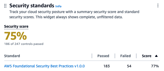
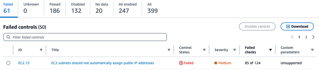
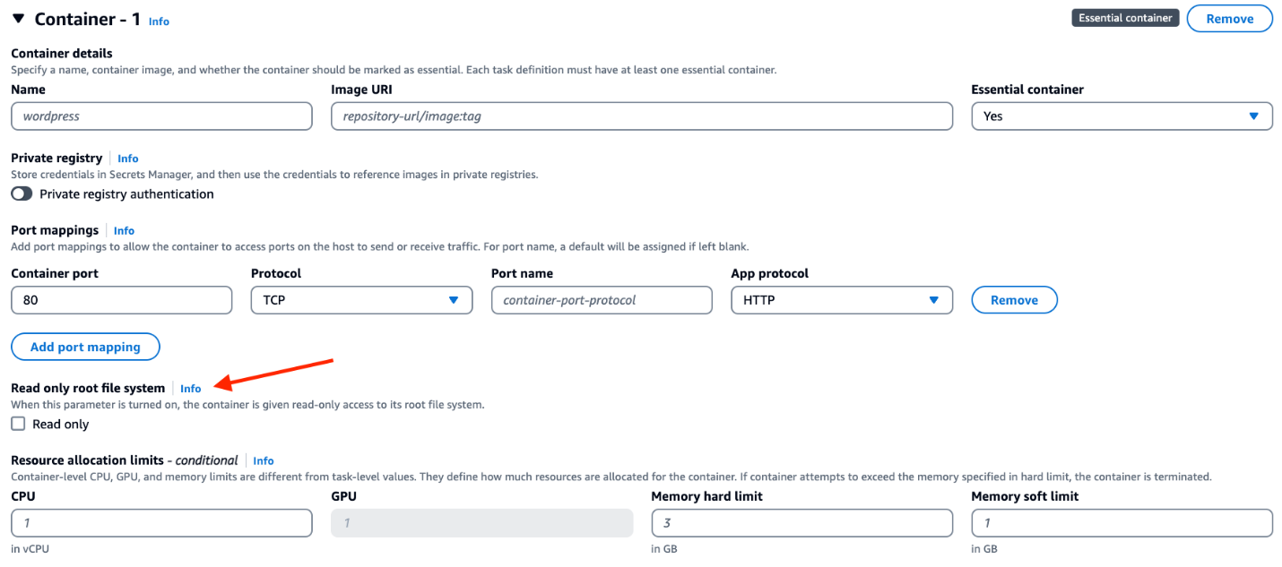


 Chaitanya Vejendla is a Senior Solutions Architect specialized in DataLake & Analytics primarily working for Healthcare and Life Sciences industry division at AWS. Chaitanya is responsible for helping life sciences organizations and healthcare companies in developing modern data strategies, deploy data governance and analytical applications, electronic medical records, devices, and AI/ML-based applications, while educating customers about how to build secure, scalable, and cost-effective AWS solutions. His expertise spans across data analytics, data governance, AI, ML, big data, and healthcare-related technologies.
 Ramesh H Singh is a Senior Product Manager Technical (External Services) at AWS in Seattle, Washington, currently with the Amazon DataZone team. He is passionate about building high-performance ML/AI and analytics products that enable enterprise customers to achieve their critical goals using cutting-edge technology.
 Rishabh Asthana is a Front-end Engineer at AWS, working with the Amazon DataZone team based in New York City, USA.
 Somdeb Bhattacharjee is an Enterprise Solutions Architect based out of New York, USA focused on helping customers on their cloud journey. He has interest in Databases, Big Data and Analytics.


 Poulomi Dasgupta is a Senior Analytics Solutions Architect with AWS. She is passionate about helping customers build cloud-based analytics solutions to solve their business problems. Outside of work, she likes travelling and spending time with her family.
 Ranjan Burman is an Analytics Specialist Solutions Architect at AWS. He specializes in Amazon Redshift and helps customers build scalable analytical solutions. He has more than 16 years of experience in different database and data warehousing technologies. He is passionate about automating and solving customer problems with cloud solutions.
 Jason Pedreza is a Senior Redshift Specialist Solutions Architect at AWS with data warehousing experience handling petabytes of data. Prior to AWS, he built data warehouse solutions at Amazon.com and Amazon Devices. He specializes in Amazon Redshift and helps customers build scalable analytic solutions.
 Agasthi Kothurkar is an AWS Solutions Architect, and is based in Boston. Agasthi works with enterprise customers as they transform their business by adopting the Cloud. Prior to joining AWS, he worked with leading IT consulting organizations on customers engagements spanning Cloud Architecture, Enterprise Architecture, IT Strategy, and Transformation. He is passionate about applying Cloud technologies to resolve complex real world business problems.


 Vijay Gopalakrishnan is a Director of Product Management with Salesforce with several years of experience in the data space. He currently is a part of the Salesforce Data Cloud team.
 Ravi Bhattiprolu is a Sr. Partner Solutions Architect at AWS. Ravi works with strategic ISV partners, Salesforce and Tableau, to deliver innovative and well-architected products and solutions that help joint customers achieve their business and technical objectives.
 Avijit Goswami is a Principal Solutions Architect at AWS specialized in data and analytics. He supports AWS strategic customers in building high-performing, secure, and scalable data lake solutions on AWS using AWS managed services and open-source solutions. Outside of his work, Avijit likes to travel, hike, watch sports, and listen to music.
 Ife Stewart is a Principal Solutions Architect in the Strategic ISV segment at AWS. She has been engaged with Salesforce Data Cloud over the last 2 years to help build integrated customer experiences across Salesforce and AWS. Ife has over 10 years of experience in technology. She is an advocate for diversity and inclusion in the technology field.
 Mike Patterson is a Senior Customer Solutions Manager in the Strategic ISV segment at AWS. He has partnered with Salesforce Data Cloud to align business objectives with innovative AWS solutions to achieve impactful customer experiences. In Mike’s spare time, he enjoys spending time with his family, sports, and outdoor activities.

 Ashok Chintalapati is a software development engineer for Amazon EMR at Amazon Web Services.
 Steve Koonce is an Engineering Manager for EMR at Amazon Web Services.

 Emmanuele Levi is a Solutions Architect in the Enterprise Software and SaaS team, based in London. Emanuele helps UK customers on their journey to refactor monolithic applications into modern microservices SaaS architectures. Emanuele is mainly interested in event-driven patterns and designs, especially when applied to analytics and AI, where he has expertise in the fraud-detection industry.
 Lorenzo Nicora is a Senior Streaming Solution Architect helping customers across EMEA. He has been building cloud-native, data-intensive systems for over 25 years, working across industries, in consultancies and product companies. He has leveraged open-source technologies extensively and contributed to several projects, including Apache Flink.
 Nicholas Tunney is a Senior Partner Solutions Architect for Worldwide Public Sector at AWS. He works with Global SI partners to develop architectures on AWS for clients in the government, nonprofit healthcare, utility, and education sectors. He is also a core member of the SaaS Technical Field Community where he gets to meet clients from all over the world who are building SaaS on AWS.


 Ritesh Kumar Sinha is an Analytics Specialist Solutions Architect based out of San Francisco. He has helped customers build scalable data warehousing and big data solutions for over 16 years. He loves to design and build efficient end-to-end solutions on AWS. In his spare time, he loves reading, walking, and doing yoga.
 Tahir Aziz is an Analytics Solution Architect at AWS. He has worked with building data warehouses and big data solutions for over 15+ years. He loves to help customers design end-to-end analytics solutions on AWS. Outside of work, he enjoys traveling and cooking.
 Omama Khurshid is an Acceleration Lab Solutions Architect at Amazon Web Services. She focuses on helping customers across various industries build reliable, scalable, and efficient solutions. Outside of work, she enjoys spending time with her family, watching movies, listening to music, and learning new technologies.
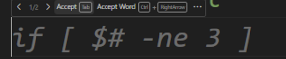
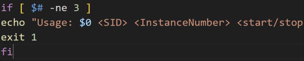
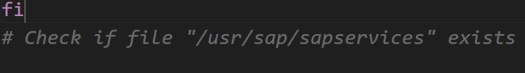
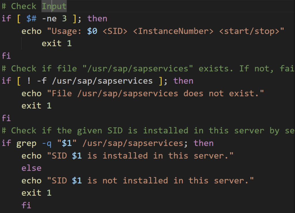
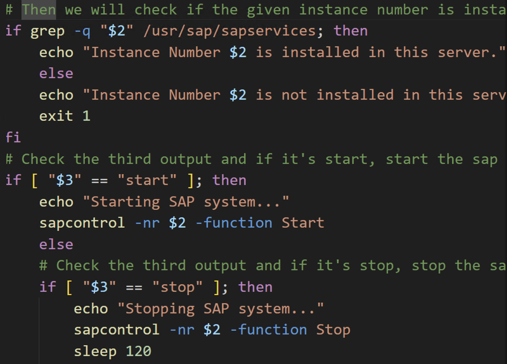
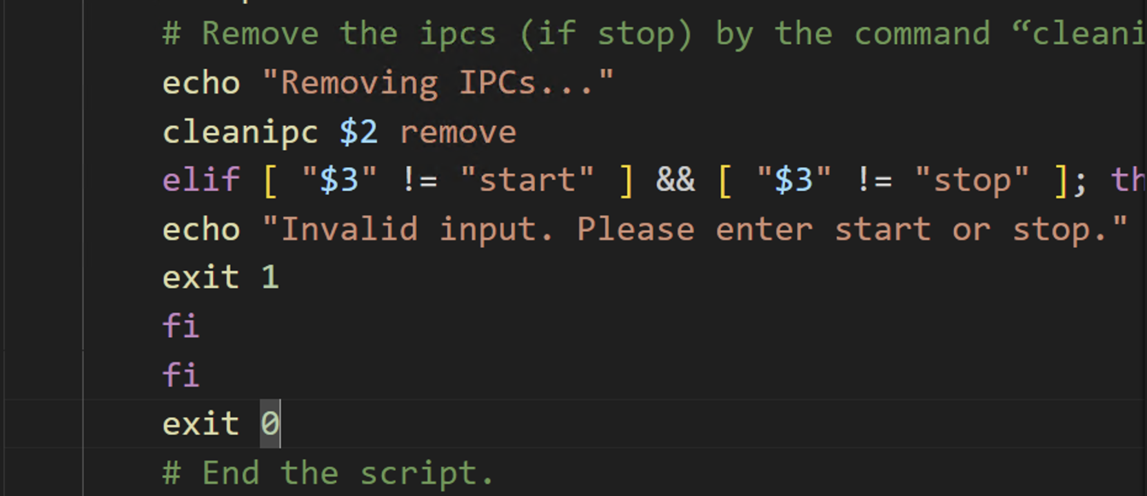
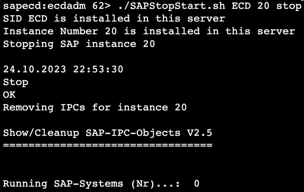


 Sharmila Shanmugam is a Solutions Architect at Amazon Web Services. She is passionate about solving the customers’ business challenges with technology and automation and reduce the operational overhead. In her current role, she helps customers across industries in their digital transformation journey and build secure, scalable, performant and optimized workloads on AWS.
 Harsh Bansal is an Analytics Solutions Architect with Amazon Web Services. In his role, he collaborates closely with clients, assisting in their migration to cloud platforms and optimizing cluster setups to enhance performance and reduce costs. Before joining AWS, he supported clients in leveraging OpenSearch and Elasticsearch for diverse search and log analytics requirements.
 Rohit Kumar works as a Cloud Support Engineer in the Support Engineering team at Amazon Web Services. He focuses on Amazon OpenSearch Service, offering guidance and technical help to customers, helping them create scalable, highly available, and secure solutions on AWS Cloud. Outside of work, Rohit enjoys watching or playing cricket. He also loves traveling and discovering new places. Essentially, his routine revolves around eating, traveling, cricket, and repeating the cycle.


 Praveen Nischal is a Cloud Software Engineer, and leads the cloud workload performance framework at Intel.
 Mulugeta Mammo is a Senior Software Engineer, and currently leads the OpenSearch Optimization team at Intel.
 Akash Shankaran is a Software Architect and Tech Lead in the Xeon software team at Intel. He works on pathfinding opportunities, and enabling optimizations for data services such as OpenSearch.
 Sarthak Aggarwal is a Software Engineer at Amazon OpenSearch Service. He has been contributing towards open-source development with indexing and storage performance as a primary area of interest.
 Prabhakar Sithanandam is a Principal Engineer with Amazon OpenSearch Service. He primarily works on the scalability and performance aspects of OpenSearch.


 Joshua Bright is a Senior Product Manager at Amazon Web Services. Joshua leads data lake integration initiatives within the OpenSearch Service team. Outside of work, Joshua enjoys listening to birds while walking in nature.


 Nihar Sheth is a Senior Product Manager at Amazon Web Services. He is passionate about developing intuitive product experiences that solve complex customer problems and enable customers to achieve their business goals.
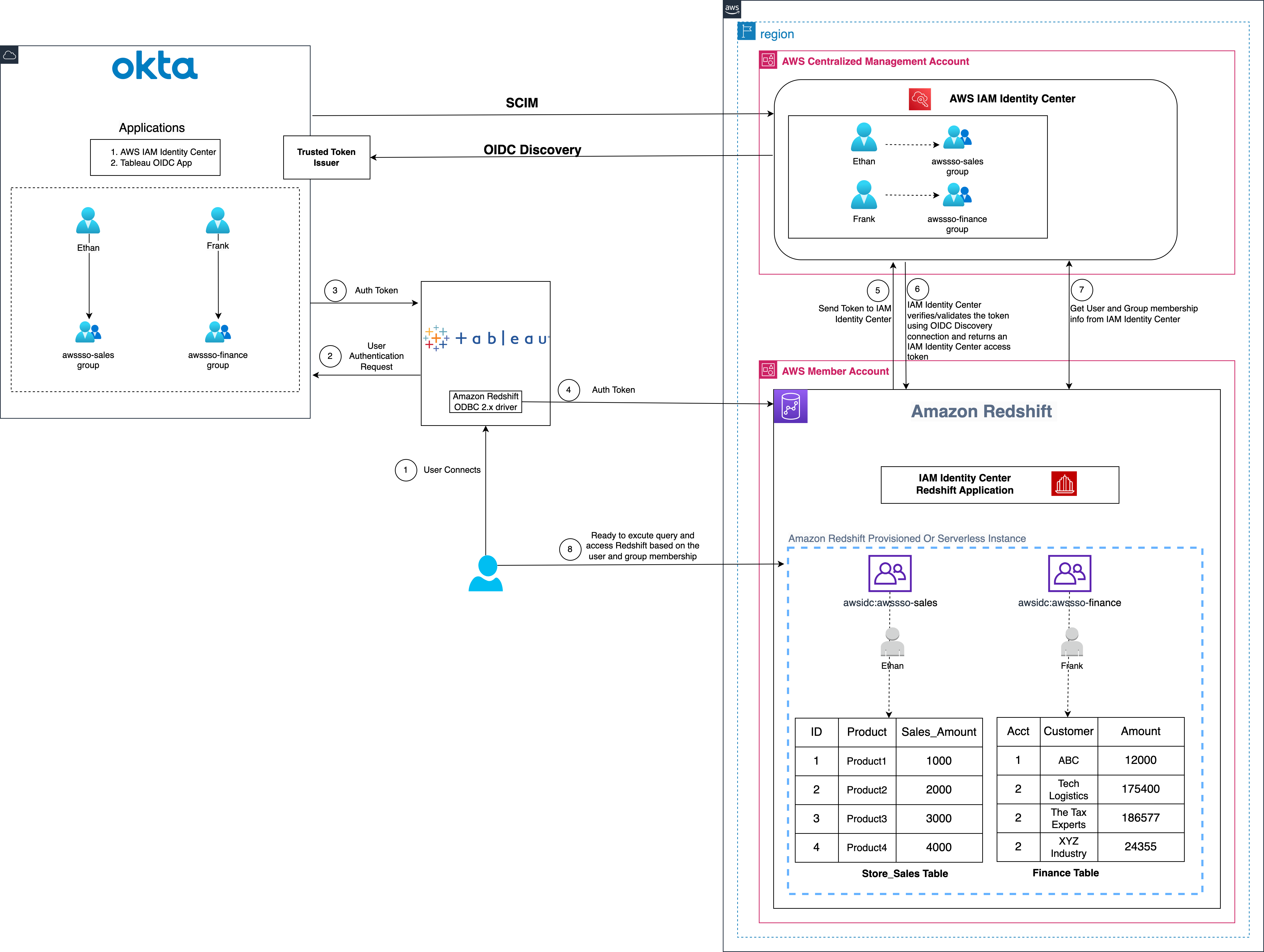


 Sid Wray is a Senior Product Manager at Salesforce based in the Pacific Northwest with nearly 20 years of experience in Digital Advertising, Data Analytics, Connectivity Integration and Identity and Access Management. He currently focuses on supporting ISV partners for Salesforce Data Cloud.
 Jade Koskela is a Principal Software Engineer at Salesforce. He has over a decade of experience building Tableau with a focus on areas including data connectivity, authentication, and identity federation.

