Tag Archives: Intermediate (200)

Build a multi-tenant healthcare system with Amazon OpenSearch Service

Post Syndicated from Ezat Karimi original https://aws.amazon.com/blogs/big-data/build-a-multi-tenant-healthcare-system-with-amazon-opensearch-service/

Healthcare systems face significant challenges managing vast amounts of data while maintaining regulatory compliance, security, and performance. This post explores strategies for implementing a multi-tenant healthcare system using Amazon OpenSearch Service.

In this context, tenants are distinct healthcare entities, sharing a common platform while maintaining isolated data environments. Hospital departments (like emergency, radiology, or patient care), clinics, insurance providers, laboratories, and research institutions are examples of these tenants.

In this post, we address common multi-tenancy challenges and provide actionable solutions for security, tenant isolation, workload management, and cost optimization across diverse healthcare tenants.

Understanding multi-tenant healthcare systems

Tenants in healthcare systems are diverse and have distinct requirements. For example, emergency departments need round-the-clock high availability with subsecond response times for patient care, along with strict access controls for sensitive trauma data. Research departments run complex, resource-intensive queries that are less time-sensitive but require robust anonymization protocols to maintain HIPAA compliance when working with patient data. Outpatient clinics operate during business hours with predictable usage patterns and moderate performance requirements. Administrative systems focus on financial data with scheduled batch processing and require access to billing information and insurance details only. Specialty departments like radiology and cardiology have unique requirements specific to the tasks they perform. For example, radiology requires high storage capacity and bandwidth for large medical imaging files, along with specialized indexing for metadata searches.

Understanding tenant requirements is essential for designing an effective multi-tenant architecture that balances resource sharing with appropriate isolation while maintaining regulatory compliance.

Isolation models

OpenSearch’s hierarchical structure consists of four main levels. At the top level is the domain, which contains one or more nodes that store and search data. Within the domain, indexes contain documents and define how they are stored and searched. Documents are individual records or data entries stored within an index, and each document consists of fields, which are individual data elements with specific data types and values.

Indexes include mappings and settings. Mappings define the schema of documents within an index, specifying field names and their data types. Settings configure various operational aspects of an index, such as the number of primary shards and replica shards.

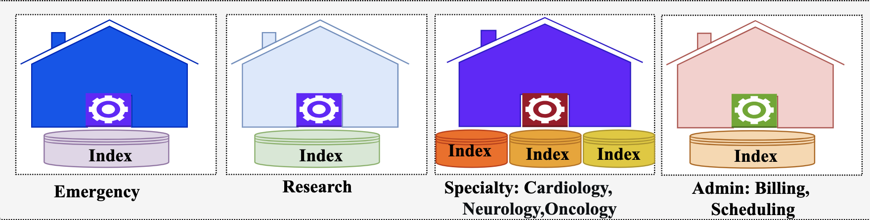
The isolation model in a multi-tenant OpenSearch system can be at domain, index, or document level. The model you select for your multi-tenant healthcare system impacts security, performance, and cost. For healthcare organizations, as depicted in the following diagram, a hybrid approach typically works best, matching isolation levels to tenant requirements.

Multi-Tenancy Isolation Models

Multi-Tenancy Isolation Models

For emergency units, consider domain-based isolation, providing maximum separation by deploying separate OpenSearch domains for each tenant. Although it’s more expensive, it reduces resource contention and provides consistent performance for critical systems. This isolation simplifies compliance by physically separating sensitive patient data.

Similarly, for clinical research tenants, consider domain-based isolation despite its higher cost. Given the resource-intensive nature of research workloads—particularly genomics and population health analytics that process terabytes of data with complex algorithms—separate domains prevent these demanding operations from impacting other tenants.

For specialty departments like cardiology or radiology, where workload patterns are similar but data access patterns are distinct, index-based isolation is a good fit. These departments share a domain but maintain separate indexes. This approach provides strong logical separation while allowing more efficient resource utilization.

For administrative departments where data is less sensitive, a document-based isolation is sufficient, and multiple tenants can share the same indexes.

Data modeling

Effective data modeling is crucial for maintaining performance and manageability in a multi-tenant healthcare system. Implement a consistent index naming convention that incorporates tenant identifiers, data categories, and time periods like {tenant-id}-{data-type}-{time-period}. Tenant-id identifies the entity, for example, cardiology. Examples of the indexes are cardiology-ecg-202505 or radiology-mri-202505. This structured approach simplifies data management, access control, and lifecycle policies.

Consider data access patterns when designing your index strategy. For example, for time-series data like vital signs or telemetry readings, time-based indexes with appropriate rotation policies will improve performance and simplify data lifecycle management.

For shared indexes using document-based isolation, make sure tenant identifiers are consistently applied and indexed for efficient tenant-based filtering.

Tenant management

Effective tenant management prevents resource contention and provides consistent performance across your healthcare system. Implement a hybrid isolation model using a tenant tiering framework based on criticality. The following table outlines the tiering framework.

Tier Tenant Type SLA Resources Operational Limits Behavior
Tier-1 Critical

Emergency departments

ICU/Critical care

Operating rooms

24/7 SLA 99.99%

Sub-second response

RPO: Near zero

RTO: Less than 15 minutes

Guaranteed 50% CPU, 50% memory

Dedicated hot nodes

2 replicas minimum

100 concurrent requests

20 MB request size

30-second timeout

No throttling

Priority query routing

Preemptive scaling

Automatic failover

Tier-2 Urgent

Inpatient units

Specialty departments

Radiology/imaging

24/7 SLA with 99.9% availability

Less than 2-second response time

RPO: Less than 15 minutes

RTO: Less than 1 hour

Guaranteed 30% CPU, 30% memory

Shared hot nodes

1–2 replicas

50 concurrent requests

15 MB request size 60-second timeout

Limited throttling during peak

High-priority query routing

Automatic scaling

Automated recovery

Tier-3 Standard

Outpatient clinics

Primary care

Pharmacy

Laboratory

Business hours SLA (8 AM – 8 PM)

99.5% availability Less than 5-second response time

RPO: Less than 1 hour

RTO: Less than 4 hours

Guaranteed 15% CPU, 15% memory

Shared nodes

1 replica

25 concurrent requests

10 MB request size

120-second timeout

Moderate throttling

Standard query routing

Fair thread allocation

Manual scaling

Business hours optimization

Tier-4 Research

Clinical research

Genomics

Population health

Best-effort

SLA, up to 99% availability

Less than 30-second response time

RPO: Less than 24 hours

RTO:  Less than 24 hours

Guaranteed 5% CPU, 10% memory

Burst capacity during off-hours

0–1 replicas

10 concurrent requests

50 MB request size

300-second timeout

Aggressive throttling during pea

Compute optimized instances

Large heap size

Research-specific plugins

Tier-5 Admin

Billing/finance

HR systems

Inventory management

Business hours SLA (9 AM – 5 PM) 99% availability Less than 10-second response time

RPO: Less than 24 hours

RTO: Less than 48 hours

No guaranteed resources

Burstable capacity

UltraWarm for historical

1 replica

5 concurrent requests

5 MB request size

180-second timeout

Aggressive throttling

Lowest priority query routing

Batch processing preferred

Off-hours scheduling

Cost-optimized storage

Workload management

When you use OpenSearch Service for multi-tenancy, you must balance your tenants’ workloads to make sure you deliver the resources needed for each to ingest, store, and query their data effectively. A multi-layered workload management framework with a rule-based proxy and OpenSearch Service workload management can effectively address these challenges. For details, see this blog post: Workload management in OpenSearch-based multi-tenant centralized logging platforms.

Security framework

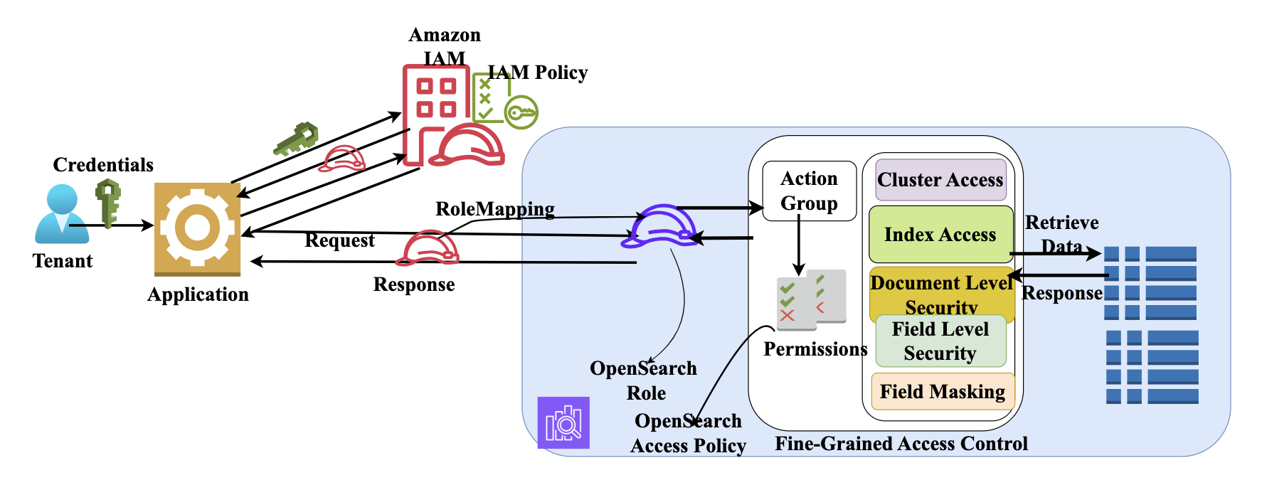
Healthcare data requires protection due to its sensitive nature and regulatory requirements. The OpenSearch Service security framework is specifically adaptable to healthcare’s strict security requirements. This framework combines multiple layers of access control, captured in the following diagram.

Multi-tenancy fine-grained access control in Amazon OpenSearch Service

Multi-tenancy fine-grained access control in Amazon OpenSearch Service

An important step in this framework is role mapping, where AWS Identity and Access Management (IAM) roles are mapped to OpenSearch roles for role-based access control (RBAC). For example, emergency departments can implement the ED-Physician role with access to patient history across departments, and the ED-Staff role with access to vital sign and medication data. You can map emergency department roles to OpenSearch roles.

With document-level security (DLS), you can limit emergency department staff to active emergency patients only while restricting access to discharged patient data only to the providers who treat them. With field-level security (FLS), you can allow access to medical fields while masking billing and insurance data. You can also provide attribute-based access control (ABAC) policies to allow access based on patient status.

For research departments, you can create Clinical-Researcher roles with read-only access to datasets. Integrate academic roles to research roles to make sure researchers only access data for studies they’re authorized to conduct. For DLS, implement filters to make sure researchers only access approved documents. Use FLS to anonymize HIPAA identifiers. For research departments, ABAC should evaluate the study phase and researcher’s location.

For outpatient care, you can define Medical-Provider roles with full access to assigned patients’ records and Medical-Assistant roles limited to documenting vitals and preliminary information. For DLS, limit access to patient’s physicians only. For FLS, restrict access to medical data only, while limiting nurses to demographic, vital signs, and medication fields. Implement time-aware ABAC policies that restrict access to patient records outside of business hours unless the provider is on-call.

For administrative departments, you can implement Financial roles with access to charge codes and insurance information but no clinical data. For DLS, make sure financial staff only access billing documents. FLS provides access to billing codes, dates of service, and insurance fields while masking clinical content.

For specialty departments, you can create technician roles like Radiologist and apply DLS filters restricting access to the data to these roles and referring physician. FLS allows technicians to see clinical history and previous findings specific to their specialty.

Enable comprehensive audit logging to track access to protected health information. Configure these logs to capture user identity, accessed data, timestamp, and access context. These audit trails are essential for regulatory compliance and security investigations.

Managing data lifecycle for compliance

Index State Management (ISM) capabilities combined with OpenSearch Service storage tiering enable an elaborate approach to data lifecycle management that can be tailored to diverse tenant needs. ISM provides a robust way to automate the lifecycle of indexes by defining policies that dictate transitions between Hot, UltraWarm, and Cold storage tiers based on criteria like index age or size. This automation can extend to the archive tier by creating snapshots, which are stored in Amazon Simple Storage Service (Amazon S3) and can be further transitioned to Amazon S3 Glacier or Glacier Deep Archive for long-term, cost-effective archiving of data that is rarely accessed.

Frame your ISM policy along the following guidelines:

Keep critical patient data in hot storage for 180 days to support immediate access. Transition to warm storage for the next 12 months, then move to cold storage for years 2–7. After 7 years, archive records.

For research data benefits, use project-based lifecycle policies rather than strictly time-based transitions. Maintain research datasets in hot storage during active project phases, regardless of data age. When projects conclude, transition data to warm storage for 12 months. Move to cold storage for the following 5–10 years based on research significance. Afterward, archive records.

For outpatient clinic data, keep recent patient records in hot storage for 90 days, aligning index rollover with typical follow-up windows. Transition to warm storage for months 4–18, coinciding with common annual visit patterns. Move to cold storage for years 2–7. Archive after 7 years.

For administrative data, maintain current fiscal year data in hot storage with automated transitions at year-end boundaries. Move previous fiscal year data to warm storage for 18 months to support auditing and reporting. Transition to cold storage for years 3–7. Archive financial records after 7 years.

For the specialty department data, keep recent metadata in hot storage for 90 days while moving large files, like images, to warm storage after 30 days. Transition complete records to cold storage after 18 months. Archive after 7 years.

Cost management and optimization

Healthcare organizations must balance performance requirements with budget constraints. Effective cost management strategies are essential for sustainable operations.

Implement comprehensive tagging strategies that mirror your index naming conventions to create a unified approach to resource management and cost tracking. Like the index naming convention, design your tags to identify the tenant, application, and data type (for example, “tenant=cardiology” or “application=ecg“). These tags, combined with AWS Cost Explorer, provide visibility into expenses across organizational boundaries.

Develop cost allocation mechanisms that fairly distribute expenses across different tenants. Consider implementing tiered pricing structures based on data volume, query complexity, and service-level guarantees. This approach aligns costs with value and encourages efficient resource utilization.

Optimize your infrastructure based on tenant-specific metrics and usage patterns. Monitor document counts, indexing rates, and query patterns to right-size your clusters and node types. Use different instance types for different workloads—for example, use compute-optimized instances for query-intensive applications.

Use OpenSearch Service storage tiering to optimize costs. UltraWarm provides significant cost savings for infrequently accessed data while maintaining reasonable query performance. Cold storage offers even greater savings for data that’s rarely accessed but must be retained for compliance purposes.

Conclusion

Building a multi-tenant healthcare system on OpenSearch Service requires careful planning and implementation. By addressing tenant isolation, security, data lifecycle management, workload control, and cost optimization, you can create a platform that delivers improved operational efficiency while maintaining strict compliance with healthcare regulations.


About the Authors

Ezat Karimi is a Senior Solutions Architect at AWS, based in Austin, TX. Ezat specializes in designing and delivering modernization solutions and strategies for database applications. Working closely with multiple AWS teams, Ezat helps customers migrate their database workloads to the AWS Cloud.

Jon Handler is a Senior Principal Solutions Architect at Amazon Web Services based in Palo Alto, CA. Jon works closely with OpenSearch and Amazon OpenSearch Service, providing help and guidance to a broad range of customers who have vector, search, and log analytics workloads that they want to move to the AWS Cloud. Prior to joining AWS, Jon’s career as a software developer included 4 years of coding a large-scale, ecommerce search engine. Jon holds a Bachelor’s of the Arts from the University of Pennsylvania, and a Master’s of Science and a PhD in Computer Science and Artificial Intelligence from Northwestern University.

Develop and deploy a generative AI application using Amazon SageMaker Unified Studio

Post Syndicated from Amit Maindola original https://aws.amazon.com/blogs/big-data/develop-and-deploy-a-generative-ai-application-using-amazon-sagemaker-unified-studio/

Picture this: You’re a financial analyst starting your Monday morning with a steaming cup of coffee, ready to review your investment portfolio. But instead of manually scouring dozens of news websites, financial reports, and industry analyses, you simply ask your AI assistant: “What global events happened over the weekend that might impact my technology stock holdings?” Within seconds, you receive a comprehensive analysis of relevant news, sentiment scores, and potential investment implications—all powered by a sophisticated generative AI application you built yourself.

This scenario isn’t science fiction; it’s the reality that modern financial professionals can create today. In an era where information moves at the speed of light and industry conditions can shift dramatically overnight, staying informed isn’t just an advantage—it’s essential for survival in competitive financial landscapes. The challenge lies in processing the overwhelming volume of global information that could impact investments while distinguishing reliable insights from noise.

Amazon SageMaker – Develop and scale AI use cases with the broadest set of tools

Luckily for us, technology is making this more straightforward. The next generation of Amazon SageMaker with Amazon SageMaker Unified Studio is a single data and AI development environment where you can find and access the data in your organization and act on it using the best tools across different use cases. SageMaker Unified Studio brings together the functionality and tools from existing AWS analytics and artificial intelligence and machine learning (AI/ML) services, including Amazon EMR , AWS Glue, Amazon Athena, Amazon Redshift , Amazon Bedrock, and Amazon SageMaker AI. From within SageMaker Unified Studio, you can find, access, and query data and AI assets across your organization, then work together in projects to securely build and share analytics and AI artifacts, including data, models, and generative AI applications.

With SageMaker Unified Studio, you can efficiently build generative AI applications in a trusted and secure environment using Amazon Bedrock. You can choose from a selection of high-performing foundation models (FMs) and advanced customization capabilities like Amazon Bedrock Knowledge Bases, Amazon Bedrock Guardrails, Amazon Bedrock Agents, and Amazon Bedrock Flows. You can rapidly tailor and deploy generative AI applications and share with the built-in catalog for discovery.

What makes SageMaker Unified Studio particularly powerful for organizations is its integration with Amazon Bedrock Flows to build generative AI workflows, which is changing how organizations think about AI application development.

Amazon Bedrock Flows for generative AI application development

With Amazon Bedrock Flows, you can build and execute complex generative AI workflows without writing code, using an intuitive visual interface that democratizes AI development. This capability is transformative for organizations where speed, accuracy, and adaptability are paramount. It offers the following benefits:

  • Visual workflow development – Users can design AI applications by dragging and dropping components onto a canvas, making AI logic transparent and modifiable
  • Business logic flexibility – The service supports complex business logic through conditional branching, multi-path decision trees, and dynamic routing
  • Democratizing AI development – Business experts can directly contribute to AI application development without requiring extensive technical expertise
  • Seamless integration – Amazon Bedrock Flows integrates with FMs, knowledge bases, guardrails, and other AWS services
  • Reduced development complexity – The service handles infrastructure management and scaling through serverless execution and SDK APIs

Solution overview

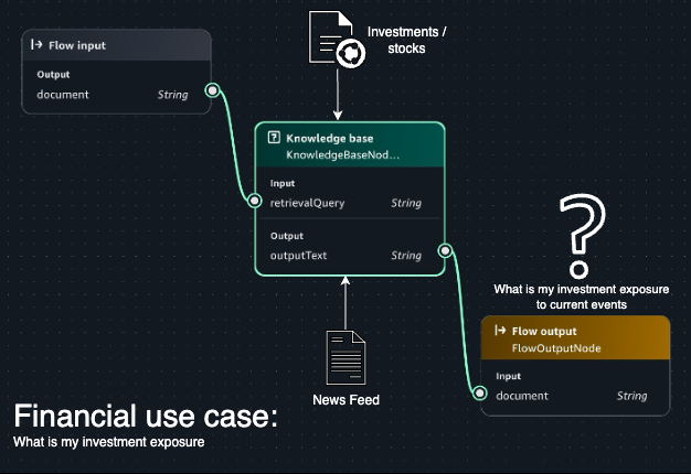
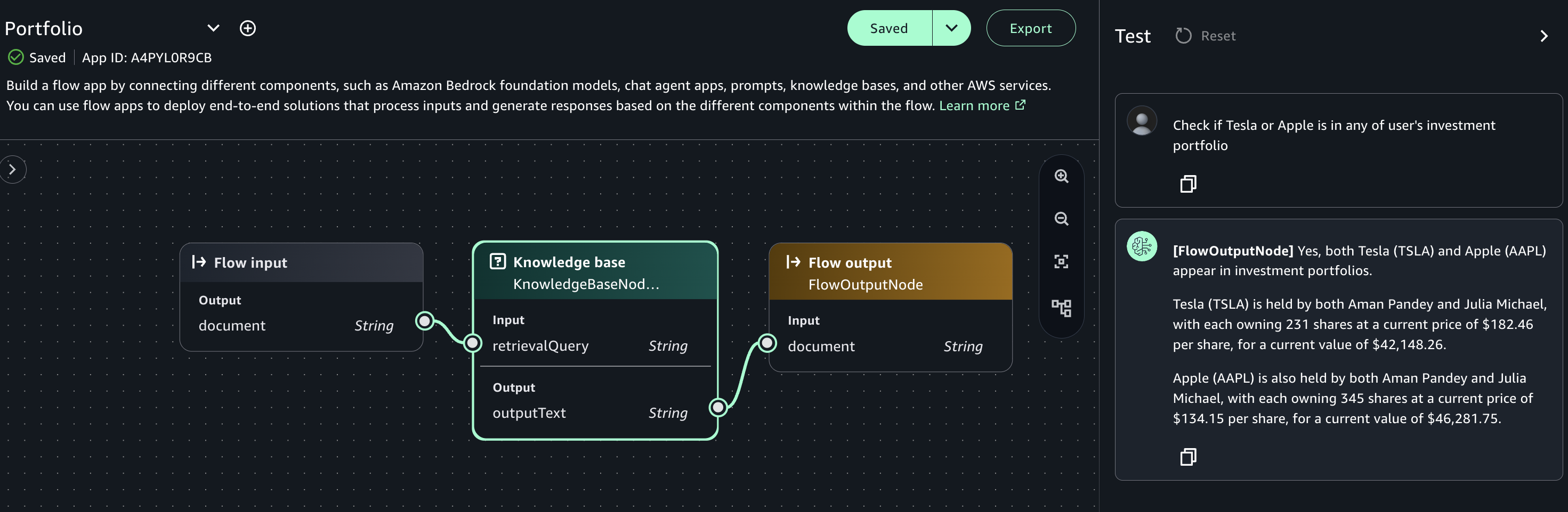
In this post, we explore a financial use case, in which we want to stay on top of latest global events and determine our investment or financial exposure based on this. We can use a SageMaker Unified Studio flow application to pull in latest news summaries, derive sentiment based on news summary, and determine their effects on my investments. The following diagram illustrates this use case.

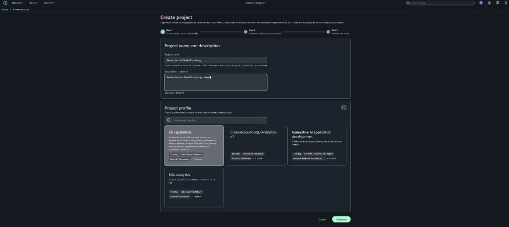
In the following sections, we show how to create a new project and build a flow application using a generative AI profile in SageMaker Unified Studio.

Prerequisites

For this walkthrough, you must have the following prerequisites:

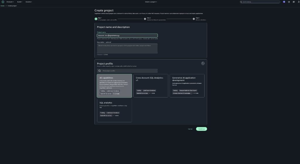
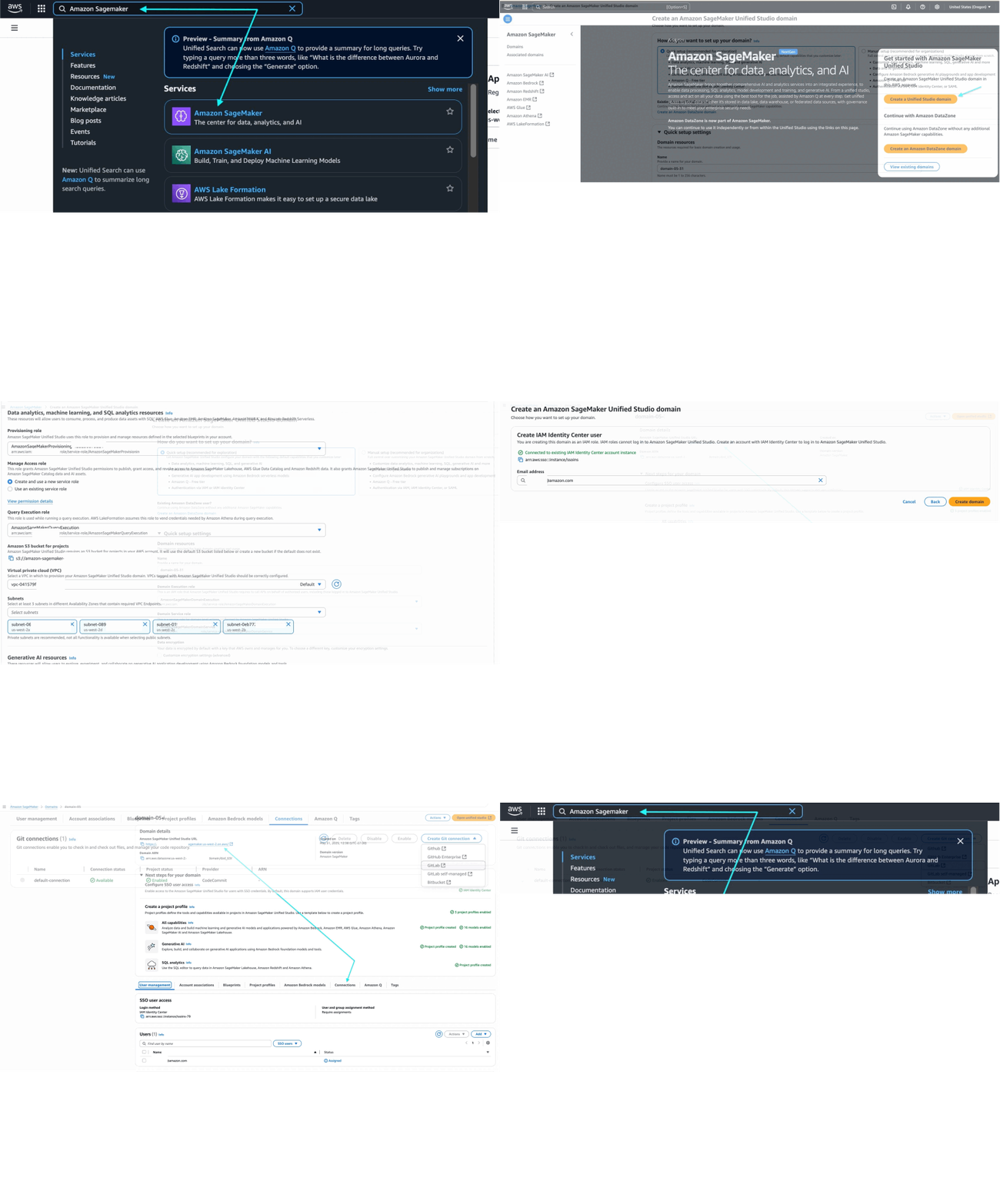
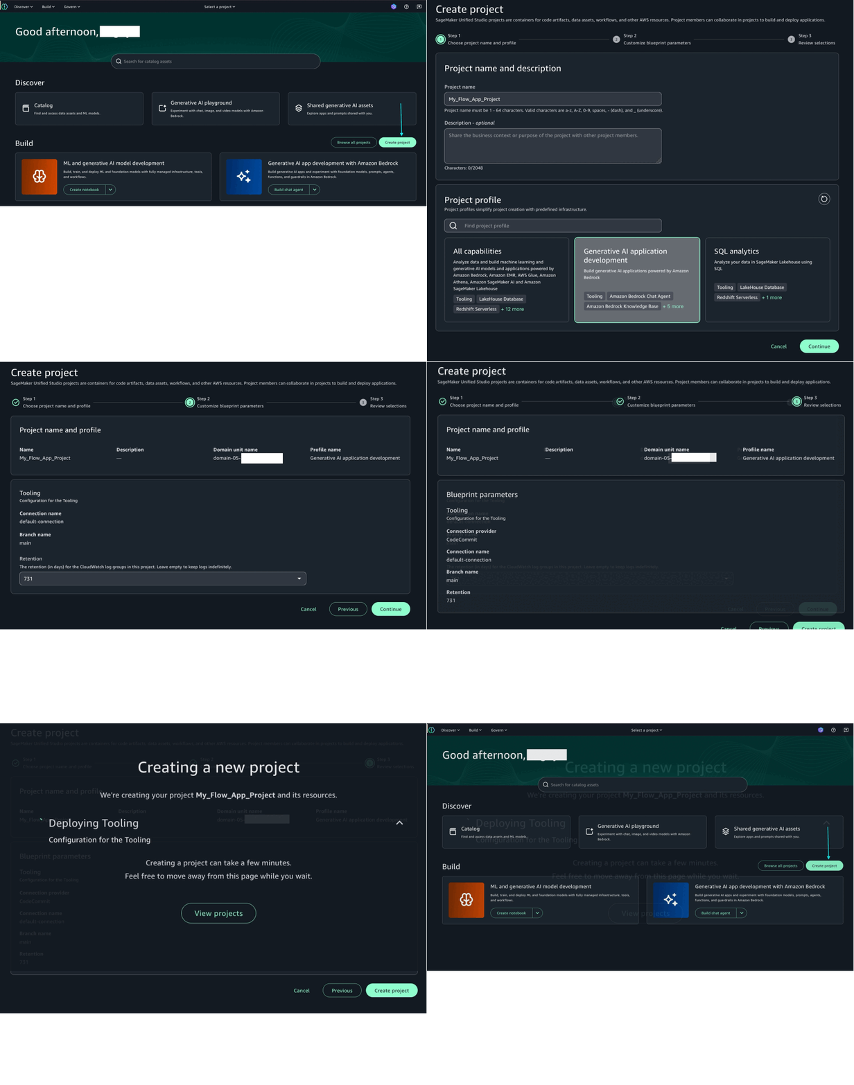
  • A demo project – Create a demo project in your SageMaker Unified Studio domain. For instructions, see Create a project. For this example, we choose All capabilities in the project profile section, which includes the generative AI project profile enabled.

Create new project and build a flow application in SageMaker Unified Studio

In this section, we create a new a flow application that uses an Amazon Bedrock knowledge base to provide information about your personal portfolio. Complete the following steps:

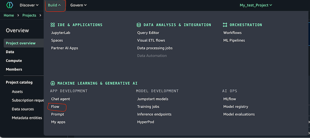
  1. In SageMaker Unified Studio, open the project you created as a prerequisite and choose Build and then Flow.

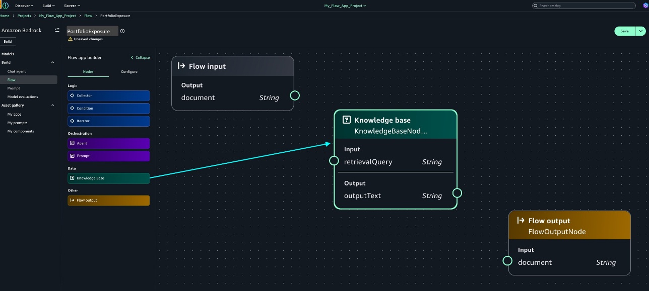
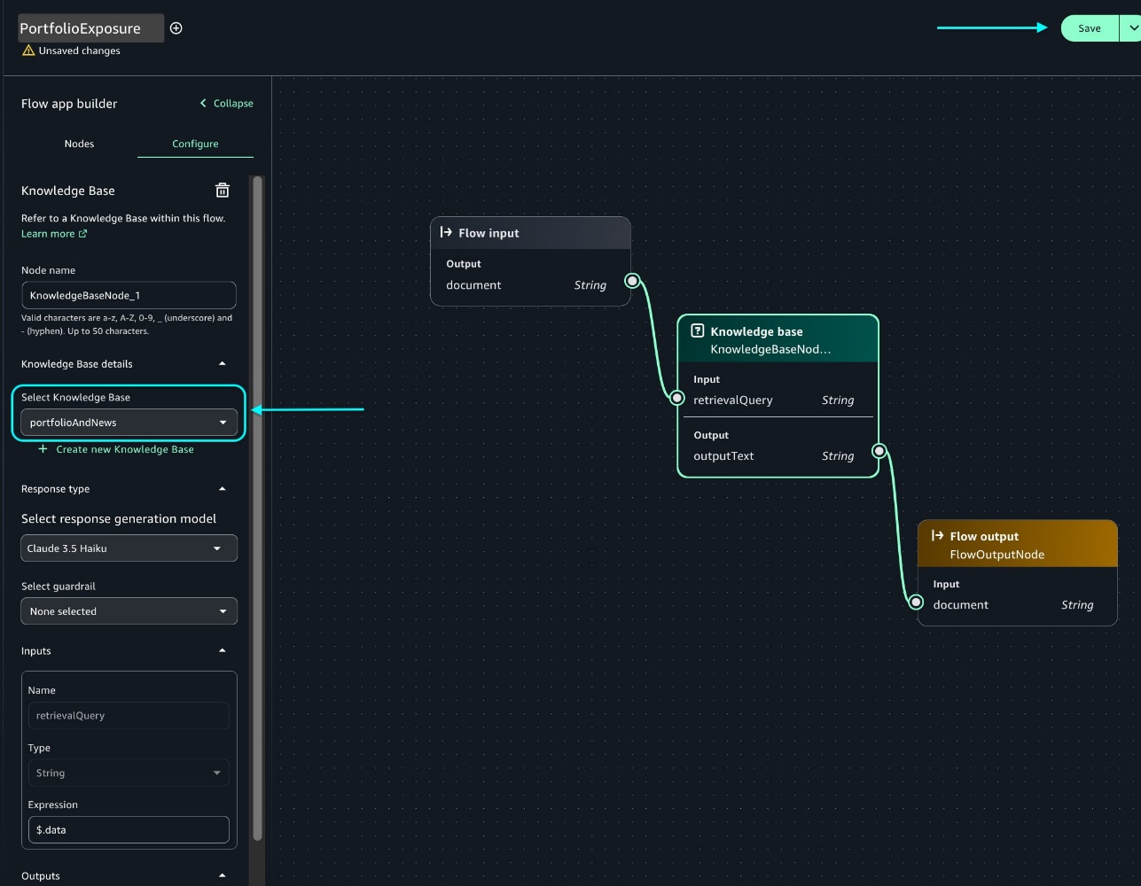
  1. Drag Knowledge Base from Nodes to the design panel to add a knowledge base that will include the user’s investment portfolio and news articles and other information like earnings call transcripts, financial analyst reports, and so on.

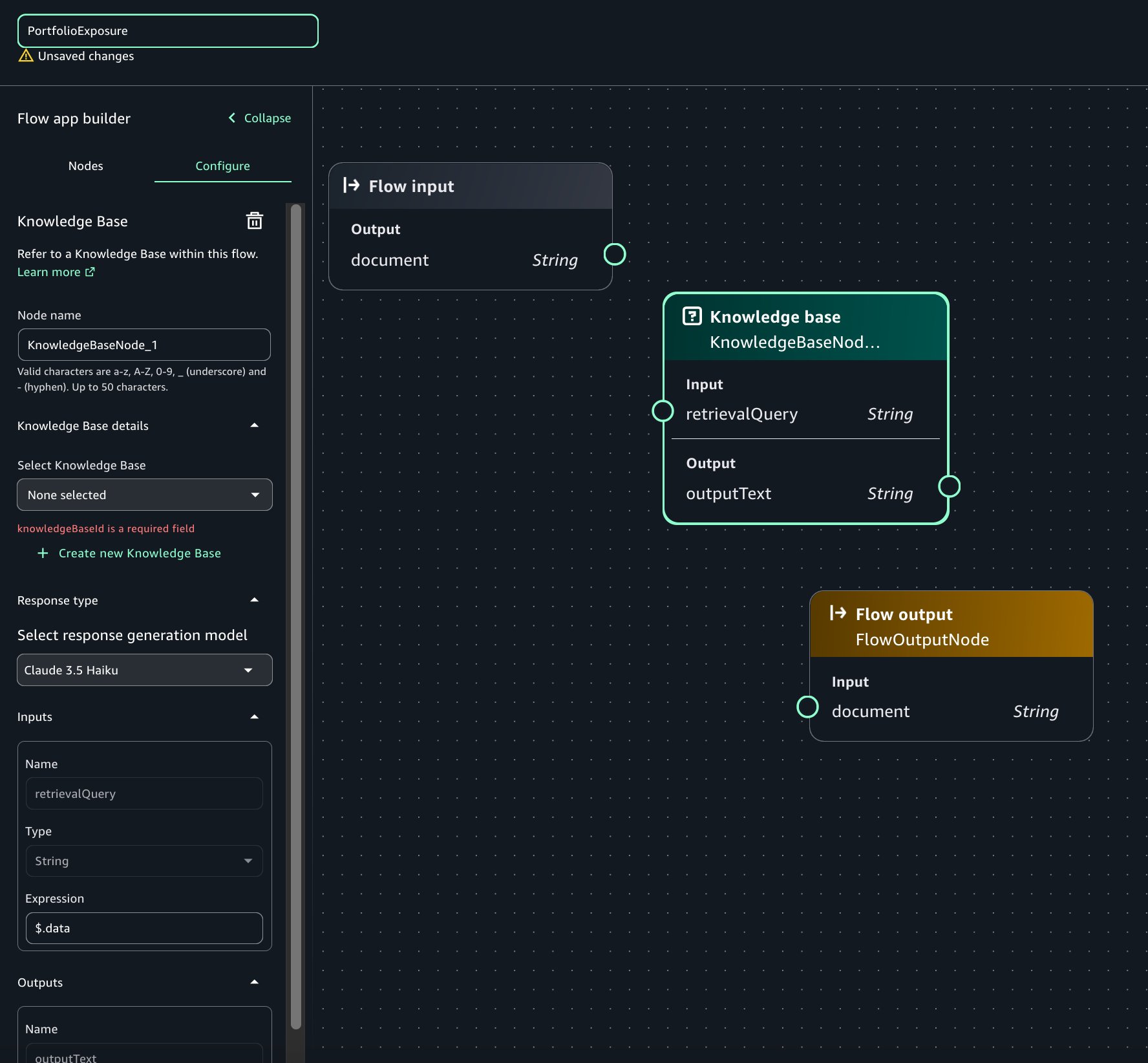
  1. Choose the Knowledge Base node and configure the knowledge base as follows:
  2. Add a name for your knowledge base name (for example, portfolio…).
  3. Choose the model (for example, Claude 3.5 Haiku).

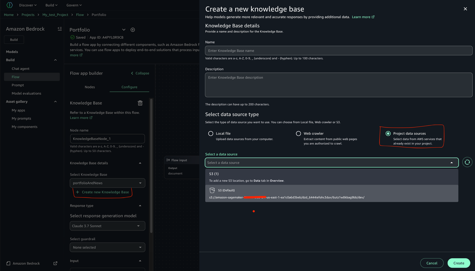
  1. Choose Create new Knowledge Base.
  2. Enter a name for the knowledge base.
  3. Select Project data source.
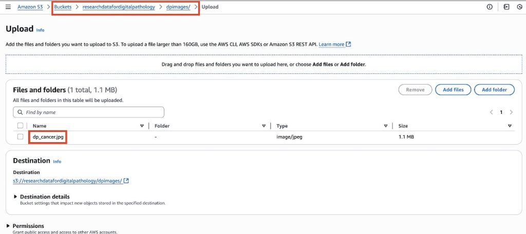
  4. For Select a data source, choose the Amazon Simple Storage Service (Amazon S3) bucket location where you uploaded your data.
  5. Choose Create.

The knowledge base creation process takes a few minutes to complete.

  1. When the knowledge base is ready, choose Save to save it to the flow.

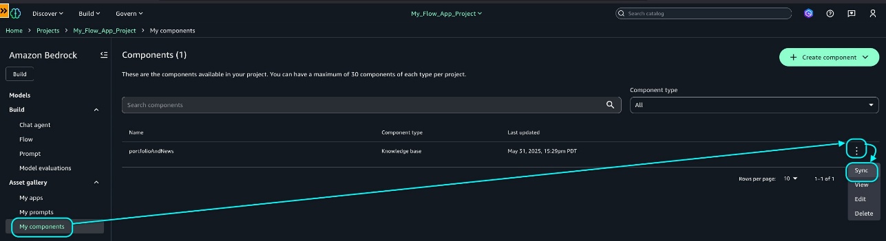
  1. Choose My components, and on the options menu (three vertical dots), choose Sync to sync the knowledge base.

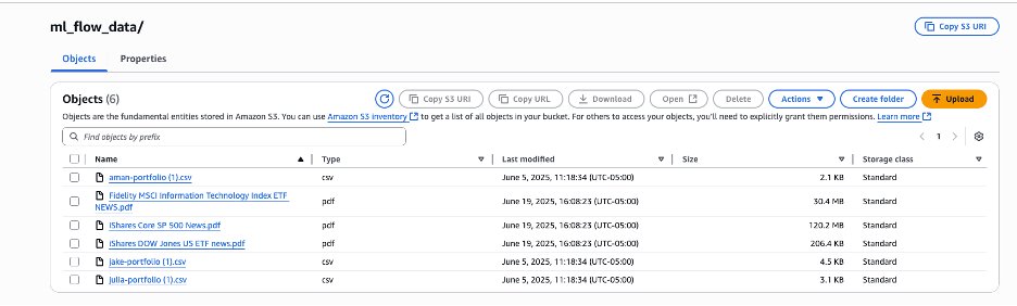
Make sure the S3 bucket has all the data (user portfolio data and latest news information data) before syncing the knowledge base.

We don’t provide any financial or news information data as part of this post. Upload current events or news data and investment portfolio data from your own data sources.

Test the flow application

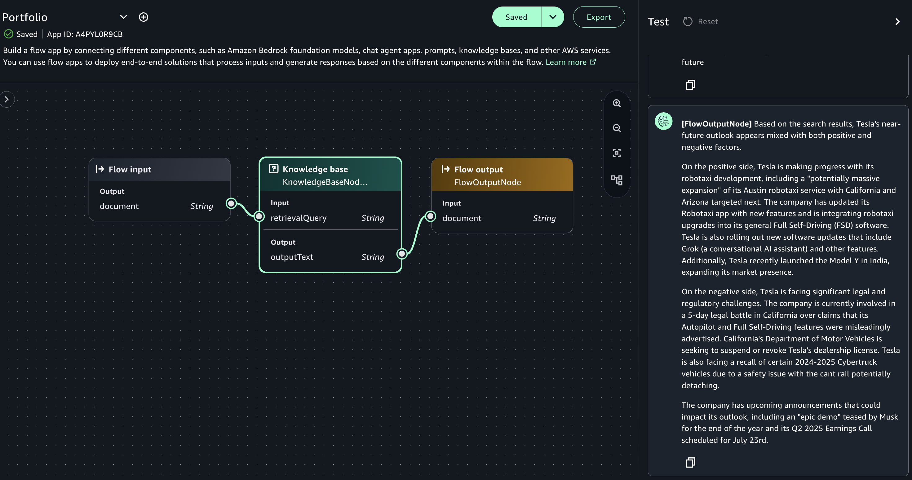
After the knowledge base sync is complete, you can return to the flow application and ask questions. Using SageMaker Unified Studio flows, a financial analyst can provide a more personalized and customized financial outlook to their customers using rich internal financial information on their customer’s investment portfolio and latest publicly available current events and news information. The following are some example questions that you can ask to test the knowledge base:

Check if Tesla or Apple is in any of user's investment portfolio

Please check latest news information to provide information if Tesla has positive, negative or neutral outlook in the near future

Flow-based applications offer a visual approach to creating complex AI workflows. By chaining different nodes, each optimized for specific functions, you can create sophisticated solutions that are more reliable, maintainable, and efficient than single-prompt approaches. These flows allow for conditional logic and branching paths, mimicking human decision-making processes and enabling more nuanced responses based on context and intermediate results.

Clean up

To avoid ongoing charges in your AWS account, delete the resources you created during this tutorial:

  1. Delete the project.
  2. Delete the domain created as part of the prerequisites.

Conclusion

In this post, we demonstrated how to use Amazon Bedrock Flows in SageMaker Unified Studio to build a sophisticated generative AI application for financial analysis and investment decision-making without extensive coding knowledge. With this integration, you can create sophisticated financial analysis workflows through an intuitive visual interface, where you can process industry data, analyze news sentiment, and assess investment implications in real time. The solution integrates seamlessly with AWS services and FMs while providing essential features like automatic scaling, compliance controls, and audit capabilities. The implementation process involves setting up a SageMaker Unified Studio domain, configuring knowledge bases with portfolio and news data, and creating visual workflows that can analyze complex financial information. This democratized approach to AI development allows both technical and business teams to collaborate effectively, significantly reducing development time while maintaining the sophisticated capabilities needed for modern financial analysis.

To get started, explore the SageMaker Unified Studio documentation, set up a project in your AWS environment, and discover how this solution can transform your organization’s data analytics capabilities.


About the authors

Amit Maindola is a Senior Data Architect focused on data engineering, analytics, and AI/ML at Amazon Web Services. He helps customers in their digital transformation journey and enables them to build highly scalable, robust, and secure cloud-based analytical solutions on AWS to gain timely insights and make critical business decisions.

Arghya Banerjee is a Sr. Solutions Architect at AWS in the San Francisco Bay Area, focused on helping customers adopt and use the AWS Cloud. He is focused on big data, data lakes, streaming and batch analytics services, and generative AI technologies.

Melody Yang is a Principal Analytics Architect for Amazon EMR at AWS. She is an experienced analytics leader working with AWS customers to provide best practice guidance and technical advice in order to assist their success in data transformation. Her areas of interests are open-source frameworks and automation, data engineering and DataOps.

Gaurav Parekh is a Solutions Architect at AWS, specializing in generative AI and data analytics, with extensive experience building production AI systems on AWS.

Introducing v2 of Powertools for AWS Lambda (Java)

Post Syndicated from Philipp Page original https://aws.amazon.com/blogs/compute/introducing-v2-of-powertools-for-aws-lambda-java/

Modern applications increasingly rely on Serverless technologies such as Amazon Web Services (AWS) Lambda to provide scalability, cost efficiency, and agility. The Serverless Applications Lens for the AWS Well-Architected Framework focuses on how to design, deploy, and architect your Serverless applications to overcome some of these challenges.

Powertools for AWS Lambda is a developer toolkit that helps you implement Serverless best practices and directly translates AWS Well-Architected recommendations into actionable, developer friendly utilities. Following the community’s continued successful adoption of Powertools for AWS in Python, Java, TypeScript, and .NET, this post announces the general availability of Powertools for AWS Lambda (Java) v2 coming with major performance improvements, enhanced core utilities, and a brand-new Kafka utility.

Powertools for AWS (Java) v2 provides three updated core utilities:

  • Logging: A re-designed Java idiomatic logging module providing structured logging that streamlines log aggregation and analysis.
  • Metrics: An improved metrics experience allowing custom metrics collection using CloudWatch Embedded Metric Format (EMF).
  • Tracing: An annotation-based way to collect distributed tracing data with AWS X-Ray to visualize and analyze request flows.

Along with the updated core utilities, v2 of the developer toolkit adds two brand new features:

  • GraalVM native image support: Native image support for GraalVM across all core utilities reducing Lambda cold start times up to 75.61% (p95).
  • Kafka utility: This new utility integrates with Amazon Managed Streaming for Apache Kafka (Amazon MSK) and self-managed Kafka event sources on Lambda and allows developers to deserialize directly into Kafka native types such as ConsumerRecords.

Learn more about how to migrate to v2 in our upgrade guide.

Getting started using Powertools for AWS Lambda (Java) v2

Powertools for AWS Lambda (Java) v2 is readily accessible as a Java package on Maven Central and integrates with popular build tools such as Maven and Gradle. This post focuses on Maven-based implementation samples to help you get started quickly. Gradle examples are available for all utilities in the documentation and the examples repository.

The toolkit is compatible with Java 11 and newer versions, making sure you can use modern Java features while building Serverless applications. Examples on how to install each utility are outlined in each section of the post and complete configuration examples are also available in the Powertools documentation.

Logging

The Logging utility helps implement structured logging when running on Lambda while still using familiar Java logging libraries such as slf4j, log4j, and logback. v2 of Logging allows you to do the following:

  • Output structured JSON logs enriched with Lambda context
  • Choose the logging backend of your choice among log4j2 and logback
  • Add structured arguments to logs that get serialized into arbitrarily nested JSON objects
  • Add global log keys using the slf4j default Mapped Diagnostic Context (MDC)

To add the logging utility to your project, include it as a dependency in your Java Maven project. The following example shows how to add the log4j2 logging backend to your application:

<!-- In the dependencies section -->
<dependency>
    <groupId>software.amazon.lambda</groupId>
    <artifactId>powertools-logging-log4j</artifactId>
    <!-- Alternatively, if you wish to use the logback backend
    <artifactId>powertools-logging-logback</artifactId> 
    -->
    <version>2.1.1</version>
</dependency>
<!-- In the build plugins section -->
<plugin>
    <groupId>dev.aspectj</groupId>
    <artifactId>aspectj-maven-plugin</artifactId>
    <configuration>
        <aspectLibraries>
            <aspectLibrary>
                <groupId>software.amazon.lambda</groupId>
                <artifactId>powertools-logging</artifactId>
                <version>2.1.1</version>
            </aspectLibrary>
        </aspectLibraries>
    </configuration>
</plugin>

Create a custom JsonTemplateLayout appender in your log4j2.xml file:

<?xml version="1.0" encoding="UTF-8"?>
<Configuration>
    <Appenders>
        <Console name="JsonAppender" target="SYSTEM_OUT">
            <JsonTemplateLayout eventTemplateUri="classpath:LambdaJsonLayout.json" />
        </Console>
    </Appenders>
    <Loggers>
        <Logger name="JsonLogger" level="INFO" additivity="false">
            <AppenderRef ref="JsonAppender"/>
        </Logger>
        <Root level="info">
            <AppenderRef ref="JsonAppender"/>
        </Root>
    </Loggers>
</Configuration>

To add structured logging to your functions, apply the @Logging annotation to your Lambda handler and use the familiar slf4j Java API when writing log statements. This allows you to adopt the logging utility without major code refactoring. Powertools handles routing to the correct logging backend for you. The following example shows how to add global log keys using MDC, and add a structured entry argument to your log message:

public class App implements RequestHandler<SQSEvent, String> {
    private static final Logger log = LoggerFactory.getLogger(App.class);

    @Logging
    public String handleRequest(final SQSEvent input, final Context context) {
        // Add a global log key using Mapped Diagnostic Context MDC
        MDC.put("myCustomKey", "willBeLoggedForAllLogStatements");

        // Log a message with a structured argument (any JSON serializable Object)
        log.info("My message", entry("anotherCustomKey", Map.of("nested", "object")));

        // ... return response
    }
}

Lambda sends the following JSON-formatted output to Amazon CloudWatch Logs (note how the Java Map gets auto-serialized into a JSON object):

{
  "level": "INFO",
  "message": "My message",
  "cold_start": true,
  "function_arn": "arn:aws:lambda:us-east-1:012345678912:function:AppFunction",
  "function_memory_size": 512,
  "function_name": "AppFunction",
  "function_request_id": "0150a2a4-c5aa-4277-9345-17bad039f6c0",
  "function_version": "$LATEST",
  "sampling_rate": 0.1,
  "service": "powertools-java-sample",
  "timestamp": "2025-05-20T08:35:28.565Z",
  "myCustomKey": "willBeLoggedForAllLogStatements",
  "anotherCustomKey": {
    "nested": "object"
  }
}

Metrics

CloudWatch offers essential built-in service metrics for monitoring application throughput, error rates, and resource usage. Users also need to capture workload specific custom metrics relevant to their business use-case following AWS Well-Architected best-practices.

Powertools for AWS (Java) enables you to create custom metrics asynchronously by outputting metrics in CloudWatch EMF directly to standard output—an approach that needs no other configuration. The Lambda service sends the EMF formatted metrics to CloudWatch on your behalf.

The Metrics utility allows you to:

  • Create custom metrics asynchronously using CloudWatch EMF
  • Reduce latency by avoiding synchronous metric publishing
  • Automatically track cold starts in a custom CloudWatch metric
  • Avoid manually validating your output against the EMF specification
  • Keep you code clean by avoiding manual flushing to standard output

To add the Metrics utility to your project, add the following Maven dependency:

<!-- In the dependencies section -->
<dependency>
    <groupId>software.amazon.lambda</groupId>
    <artifactId>powertools-metrics</artifactId>
    <version>2.1.1</version>
</dependency>
<!-- In the build plugins section -->
<plugin>
    <groupId>dev.aspectj</groupId>
    <artifactId>aspectj-maven-plugin</artifactId>
    <configuration>
        <aspectLibraries>
            <aspectLibrary>
                <groupId>software.amazon.lambda</groupId>
                <artifactId>powertools-metrics</artifactId>
                <version>2.1.1</version>
            </aspectLibrary>
        </aspectLibraries>
    </configuration>
</plugin>

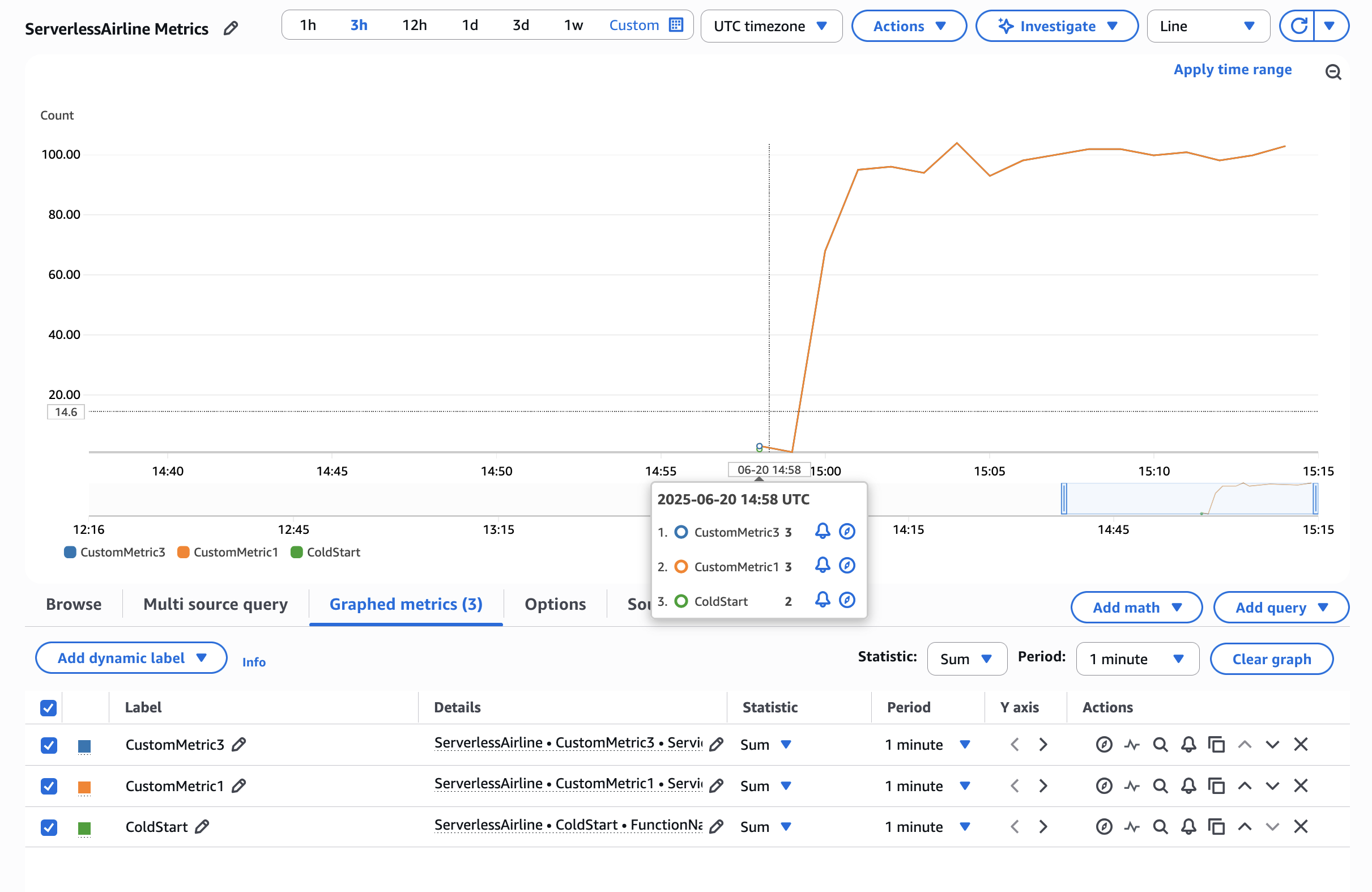
To add custom metrics to your Lambda function, place the @FlushMetrics annotation on your Lambda handler. The library takes care of validating and flushing your metrics to standard output before the Lambda function terminates. The following example shows how you can automatically capture a cold start metric and emit your own custom metrics:

public class App implements RequestHandler<SQSEvent, String> {
    private static final Logger log = LoggerFactory.getLogger(App.class);
    private static final Metrics metrics = MetricsFactory.getMetricsInstance();

    // This configures a default namespace and service dimension for all metrics
    @FlushMetrics(namespace = "ServerlessAirline", service = "payment", captureColdStart = true)
    public String handleRequest(final SQSEvent input, final Context context) {
        // The Metrics instance is a singleton
        metrics.addMetric("CustomMetric1", 1, MetricUnit.COUNT);

        // Publish metrics with non-default configuration options
        DimensionSet dimensionSet = new DimensionSet();
        dimensionSet.addDimension("Service", "AnotherService");
        metrics.flushSingleMetric("CustomMetric2", 1, MetricUnit.COUNT, "AnotherNamespace", dimensionSet);

        // ... return response
    }
}
AWS CloudWatch Metrics Graph View of metrics generated by Metrics utility example.

Figure 1. AWS CloudWatch Metrics Graph View

Tracing

The Tracing utility provides an annotation-based integration with X-Ray for distributed tracing with minimal configuration. Tracing allows you to:

  • Gain visibility into your own methods calls and AWS service interactions visualized in the X-Ray console
  • Automatically capture method responses and errors
  • Automatically capture Lambda cold start information as part of your traces
  • Add custom metadata to traces for more context and debugging information
  • Enable or disable tracing features through environment variables without code changes

To add the Tracing utility to your project, add the following Maven dependency:

<!-- In the dependencies section -->
<dependency>
    <groupId>software.amazon.lambda</groupId>
    <artifactId>powertools-tracing</artifactId>
    <version>2.1.1</version>
</dependency>
<!-- In the build plugins section -->
<plugin>
    <groupId>dev.aspectj</groupId>
    <artifactId>aspectj-maven-plugin</artifactId>
    <configuration>
        <aspectLibraries>
            <aspectLibrary>
                <groupId>software.amazon.lambda</groupId>
                <artifactId>powertools-tracing</artifactId>
                <version>2.1.1</version>
            </aspectLibrary>
        </aspectLibraries>
    </configuration>
</plugin>

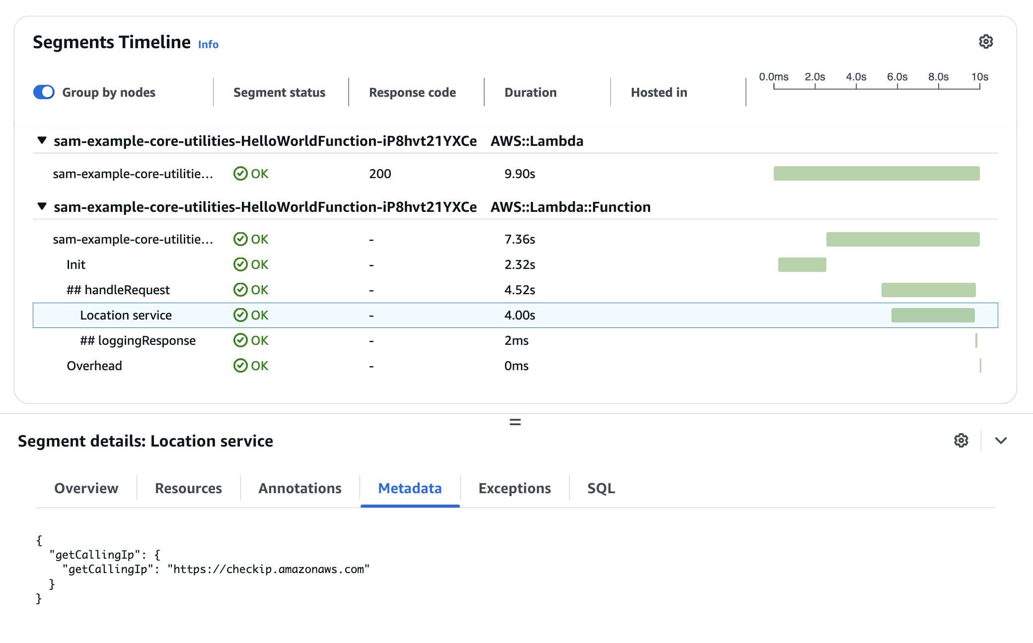
To enable tracing in your Lambda function, annotate your Lambda handler and your custom methods that you want to trace with the @Tracing annotation. Each annotation maps to a sub-segment of your main Lambda handler in X-Ray and becomes visible in the console.

public class App implements RequestHandler<APIGatewayProxyRequestEvent, APIGatewayProxyResponseEvent> {
    private static final Logger log = LoggerFactory.getLogger(App.class);

    @Tracing
    public APIGatewayProxyResponseEvent handleRequest(final APIGatewayProxyRequestEvent input, final Context context) {
        // ... business logic
        
        // Get calling IP with tracing
        String location = getCallingIp("https://checkip.amazonaws.com");

        // ... return response
    }

    @Tracing(segmentName = "Location service")
    private String getCallingIp(String address) {
        // Implementation to get IP address
        log.info("Retrieving caller IP address");
        
        // Add custom metadata to current sub-segment
        URL url = new URL(address);
        putMetadata("getCallingIp", address);
        
        // ...
        return "127.0.0.1";
    }
}

The X-Ray console displays a generated service map when traffic begins flowing through your application. Applying the Tracing annotation to your Lambda function handler method or any other methods in the execution chain provides you with comprehensive visibility into the traffic patterns throughout your application. The following figure shows how the custom metadata added in the example is associated with the custom sub-segment.

Picture showing the generated traces in the AWS X-Ray console. Shows the custom named Location service trace along with its metadata as a JSON object.

Figure 2. AWS X-Ray waterfall trace view

Reducing Lambda cold start duration

A key feature in Powertools for AWS Lambda (Java) v2 is GraalVM native image support for all core utilities. Compiling your Lambda functions to native executables allows you to significantly reduce cold start times and memory usage. Using Powertools v2 with GraalVM allows you to reduce cold starts up to 75.61% (p95) compared to using the managed Java runtime. The following benchmark compares the cold start times of an application using all core utilities (logging, metrics, tracing) on the managed java21 runtime as compared to the Lambda provided.al2023 runtime running a GraalVM compiled native image (go to the supported Lambda runtimes):

Environment p95 (ms) Min (ms) Avg (ms) Max (ms) Max Memory (MB) N
Powertools for AWS (Java) v2: JVM 1682.92 1224.55 1224.55 2229.81 205.04 234
Powertools for AWS (Java) v2: GraalVM 542.86 404.92 504.77 752.85 93.46 369

This improvement is particularly valuable for latency-sensitive applications and functions that scale frequently. Check out a full working example on GitHub.

Lambda MSK Event Source Mapping Integration

The new Kafka utility introduced with Powertools for AWS Lambda (Java) v2 streamlines working with the Lambda MSK Event Source Mapping (ESM) and self-managed Kafka event sources. It provides a familiar experience for developers working with Apache Kafka by allowing direct conversion from Lambda events to Kafka’s native types. The key features include:

  • Direct deserialization into Kafka ConsumerRecords<K, V> objects while using the Lambda-native RequestHandler interface
  • Support for deserializing JSON, Avro, and Protobuf encoded records for key and value fields with and without usage of a Schema Registry when producing the messages

To add the Kafka utility to your project, include the powertools-kafka library as a Maven dependency in your pom.xml:

<!-- In the dependencies section -->
<dependency>
    <groupId>software.amazon.lambda</groupId>
    <artifactId>powertools-kafka</artifactId>
    <version>2.1.1</version>
</dependency>
<!-- Kafka clients dependency - compatibility works for >= 3.0.0 -->
<dependency>
    <groupId>org.apache.kafka</groupId>
    <artifactId>kafka-clients</artifactId>
    <version>4.0.0</version>
</dependency>

Use the @Deserialization annotation on your Lambda handler to deserialize messages as native Kafka ConsumerRecords. Make sure to specify the deserializer type. The following example shows how to deserialize Avro encoded record values with String keys. As in a regular Lambda handler, declare the input type to your function in the RequestHandler generic parameters and the utility discovers the deserialization types automatically. The AvroProduct class in the following example is an auto-generated Java class using the Java org.apache.avro.avro library.

public class App implements RequestHandler<ConsumerRecords<String, AvroProduct>, Void> {
    private static final Logger log = LoggerFactory.getLogger(App.class);

    @Deserialization(type = DeserializationType.KAFKA_AVRO)
    public Void handleRequest(ConsumerRecords<String, AvroProduct> consumerRecords, Context context) {
        log.info("Deserialized {} records.", consumerRecords.records().size()); 

        // ... Business logic 
        
        return null;
    }
}

Conclusion

Powertools for AWS Lambda (Java) v2 represents the next evolution in the toolkit for building robust, observable, and high-performing Serverless applications. Throughout this post, we’ve explored the enhanced core observability utilities with their new features, the performance gains through GraalVM native image support, and the new Kafka utility that supports using familiar Kafka patterns when working on Lambda.

Powertools also offers more utilities to handle common Serverless design patterns. Each utility is designed with the same principles of clarity and minimal overhead.To learn more:

  1. Visit the documentation for detailed guides and examples
  2. Try the sample applications
  3. Join the community on GitHub to share your experience and get help

Your next Serverless application awaits with Powertools for AWS Lambda (Java) v2. We would love to hear your feedback!

Build an analytics pipeline that is resilient to Avro schema changes using Amazon Athena

Post Syndicated from Mohammad Sabeel original https://aws.amazon.com/blogs/big-data/build-an-analytics-pipeline-that-is-resilient-to-avro-schema-changes-using-amazon-athena/

As technology progresses, the Internet of Things (IoT) expands to encompass more and more things. As a result, organizations collect vast amounts of data from diverse sensor devices monitoring everything from industrial equipment to smart buildings. These sensor devices frequently undergo firmware updates, software modifications, or configuration changes that introduce new monitoring capabilities or retire obsolete metrics. As a result, the data structure (schema) of the information transmitted by these devices evolves continuously.

Organizations commonly choose Apache Avro as their data serialization format for IoT data due to its compact binary format, built-in schema evolution support, and compatibility with big data processing frameworks. This becomes crucial when sensor manufacturers release updates that add new metrics or deprecate old ones, allowing for seamless data processing. For example, when a sensor manufacturer releases a firmware update that adds new temperature precision metrics or deprecates legacy vibration measurements, Avro’s schema evolution capabilities allow for seamless handling of these changes without breaking existing data processing pipelines.

However, managing schema evolution at scale presents significant challenges. For example, organizations need to store and process data from thousands of sensors and update their schemas independently, handle schema changes occurring as frequently as every hour due to rolling device updates, maintain historical data compatibility while accommodating new schema versions, query data across multiple time periods with different schemas for temporal analysis, and ensure minimal query failures due to schema mismatches.

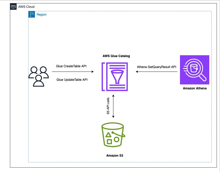
To address this challenge, this post demonstrates how to build such a solution by combining Amazon Simple Storage Service (Amazon S3) for data storage, AWS Glue Data Catalog for schema management, and Amazon Athena for one-time querying. We’ll focus specifically on handling Avro-formatted data in partitioned S3 buckets, where schemas can change frequently while providing consistent query capabilities across all data regardless of schema versions.

This solution is specifically designed for Hive-based tables, such as those in the AWS Glue Data Catalog, and is not applicable for Iceberg tables. By implementing this approach, organizations can build a highly adaptive and resilient analytics pipeline capable of handling extremely frequent Avro schema changes in partitioned S3 environments.

Solution overview

In this post as an example, we’re simulating a real-world IoT data pipeline with the following requirements:

  • IoT devices continuously upload sensor data in Avro format to an S3 bucket, simulating real-time IoT data ingestion
  • The schema change happens frequently over time
  • Data will be partitioned hourly to reflect typical IoT data ingestion patterns
  • Data needs to be queryable using the most recent schema version through Amazon Athena.

To achieve these requirements, we demonstrate the solution using automated schema detection. We use AWS Command Line Interface (AWS CLI) and AWS SDK for Python (Boto3) scripts to simulate an automated mechanism that continually monitors the S3 bucket for new data, detects schema changes in incoming Avro files, and triggers necessary updates to the AWS Glue Data Catalog.

For schema evolution handling, our solution will demonstrate how to create and update table definitions in the AWS Glue Data Catalog, incorporate Avro schema literals to handle schema changes, and use the Athena partition projection for efficient querying across schema versions. The data steward or admin needs to know when and how the schema is updated so that the admin can manually change the columns in the UpdateTable API call. For validation and querying, we use Amazon Athena queries to verify table definitions and partition details and demonstrate successful querying of data across different schema versions. By simulating these components, our solution addresses the key requirements outlined in the introduction:

  • Handling frequent schema changes (as often as hourly)
  • Managing data from thousands of sensors updating independently
  • Maintaining historical data compatibility while accommodating new schemas
  • Enabling querying across multiple time periods with different schemas
  • Minimizing query failures due to schema mismatches

Although in a production environment this would be integrated into a sophisticated IoT data processing application, our simulation using AWS CLI and Boto3 scripts effectively demonstrates the principles and techniques for managing schema evolution in large-scale IoT deployments.

The following diagram illustrates the solution architecture.

Prerequisites:

To perform the solution, you need to have the following prerequisites:

Create the base table

In this section, we simulate the initial setup of a data pipeline for IoT sensor data. This step is crucial because it establishes the foundation for our schema evolution demonstration. This initial table serves as the starting point from which our schema will evolve. It allows us to demonstrate how to handle schema changes over time. In this scenario, the base table contains three key fields: customerID (bigint), sentiment (a struct containing customerrating), and dt (string) as a partition column. And Avro schema literal (‘avro.schema.literal’)along with other configurations. Follow these steps:

  1. Create a new file named `CreateTableAPI.py` with the following content. Replace 'Location': 's3://amzn-s3-demo-bucket/' with your S3 bucket details and <AWS Account ID> with your AWS account ID:
import boto3
import time

if __name__ == '__main__':
    database_name = " blogpostdatabase"
    table_name = "blogpost_table_test"
    catalog_id = ''
    client = boto3.client('glue')

    response = client.create_table(
        CatalogId=catalog_id,
        DatabaseName=database_name,
        TableInput={
            'Name': table_name,
            'Description': 'sampletable',
            'Owner': 'root',
            'TableType': 'EXTERNAL_TABLE',
            'LastAccessTime': int(time.time()),
            'LastAnalyzedTime': int(time.time()),
            'Retention': 0,
            'Parameters' : {
                'avro.schema.literal': '{"type" : "record", "name" : "customerdata", "namespace" : "com.data.test.avro", "fields" : [{ "name" : "customerID", "type" : "long", "default" : -1 },{ "name" : "sentiment", "type" : [ "null", { "type" : "record", "name" : "sentiment", "doc" : "***** CoreETL ******", "fields" : [ { "name" : "customerrating", "type" : "long", "default" : 0 }] } ], "default" : 0 }]}'
            },
            'StorageDescriptor': {
                'Columns': [
                    {
                        'Name': 'customerID',
                        'Type': 'bigint',
                        'Comment': 'from deserializer'
                    },
                    {
                        'Name': 'sentiment',
                        'Type': 'struct<customerrating:bigint>',
                        'Comment': 'from deserializer'
                    }
                ],
                'Location': 's3:///',
                'InputFormat': 'org.apache.hadoop.hive.ql.io.avro.AvroContainerInputFormat',
                'OutputFormat': 'org.apache.hadoop.hive.ql.io.avro.AvroContainerOutputFormat',
                'SerdeInfo': {
                    'SerializationLibrary': 'org.apache.hadoop.hive.serde2.avro.AvroSerDe',
                    'Parameters': {
                        'avro.schema.literal': '{"type" : "record", "name" : "customerdata", "namespace" : "com.data.test.avro", "fields" : [{ "name" : "customerID", "type" : "long", "default" : -1 },{ "name" : "sentiment", "type" : [ "null", { "type" : "record", "name" : "sentiment", "doc" : "***** CoreETL ******", "fields" : [ { "name" : "customerrating", "type" : "long", "default" : 0 } ] } ], "default" : 0 }]}'
                    }
                }
            },
            'PartitionKeys': [
                {
                    'Name': 'dt',
                    'Type': 'string'
                }
            ]
        }
    )

    print(response)
  1. Run the script using the command:
python3 CreateTableAPI.py

The schema literal serves as a form of metadata, providing a clear description of your data structure. In Amazon Athena, Avro table schema Serializer/Deserializer (SerDe) properties are essential for schema is compatible with the data stored in files, facilitating accurate translation for query engines. These properties enable the precise interpretation of Avro-formatted data, allowing query engines to correctly read and process the information during execution.

The Avro schema literal provides a detailed description of the data structure at the partition level. It defines the fields, their data types, and any nested structures within the Avro data. Amazon Athena uses this schema to correctly interpret the Avro data stored in Amazon S3. It makes sure that each field in the Avro file is mapped to the correct column in the Athena table.

The schema information helps Athena optimize query run by understanding the data structure in advance. It can make informed decisions about how to process and retrieve data efficiently. When the Avro schema changes (for example, when new fields are added), updating the schema literal allows Athena to recognize and work with the new structure. This is crucial for maintaining query compatibility as your data evolves over time. The schema literal provides explicit type information, which is essential for Avro’s type system. This provides accurate data type conversion between Avro and Athena SQL types.

For complex Avro schemas with nested structures, the schema literal informs Athena how to navigate and query these nested elements. The Avro schema can specify default values for fields, which Athena can use when querying data where certain fields might be missing. Athena can use the schema to perform compatibility checks between the table definition and the actual data, helping to identify potential issues. In the SerDe properties, the schema literal tells the Avro SerDe how to deserialize the data when reading it from Amazon S3.

It’s crucial for the SerDe to correctly interpret the binary Avro format into a form Athena can query. The detailed schema information aids in query planning, allowing Athena to make informed decisions about how to execute queries efficiently. The Avro schema literal specified in the table’s SerDe properties provides Athena with the exact field mappings, data types, and physical structure of the Avro file. This enables Athena to perform column pruning by calculating precise byte offsets for required fields, reading only those specific portions of the Avro file from S3 rather than retrieving the entire record.

Parameters' : {
                'avro.schema.literal': '{"type" : "record", "name" : "customerdata", "namespace" : "com.data.test.avro", "fields" : [{ "name" : "customerID", "type" : "long", "default" : -1 },{ "name" : "sentiment", "type" : [ "null", { "type" : "record", "name" : "sentiment", "doc" : "***** CoreETL ******", "fields" : [ { "name" : "customerrating", "type" : "long", "default" : 0 }] } ], "default" : 0 }]}'
            },
  1. After creating the table, verify its structure using the SHOW CREATE TABLE command in Athena:
CREATE EXTERNAL TABLE `blogpost_table_test`(
  `customerid` bigint COMMENT 'from deserializer', 
  `sentiment` struct<customerrating:bigint> COMMENT 'from deserializer')
PARTITIONED BY ( 
  `dt` string)
ROW FORMAT SERDE 
  'org.apache.hadoop.hive.serde2.avro.AvroSerDe' 
WITH SERDEPROPERTIES ( 
  'avro.schema.literal'='{\"type\" : \"record\", \"name\" : \"customerdata\", \"namespace\" : \"com.data.test.avro\", \"fields\" : [{ \"name\" : \"customerID\", \"type\" : \"long\", \"default\" : -1 },{ \"name\" : \"sentiment\", \"type\" : [ \"null\", { \"type\" : \"record\", \"name\" : \"sentiment\", \"doc\" : \"***** CoreETL ******\", \"fields\" : [ { \"name\" : \"customerrating\", \"type\" : \"long\", \"default\" : 0 } ] } ], \"default\" : 0 }]}') 
STORED AS INPUTFORMAT 
  'org.apache.hadoop.hive.ql.io.avro.AvroContainerInputFormat' 
OUTPUTFORMAT 
  'org.apache.hadoop.hive.ql.io.avro.AvroContainerOutputFormat'
LOCATION
  's3://amzn-s3-demo-bucket/'
TBLPROPERTIES (
  'avro.schema.literal'='{\"type\" : \"record\", \"name\" : \"customerdata\", \"namespace\" : \"com.data.test.avro\", \"fields\" : [{ \"name\" : \"customerID\", \"type\" : \"long\", \"default\" : -1 },{ \"name\" : \"sentiment\", \"type\" : [ \"null\", { \"type\" : \"record\", \"name\" : \"sentiment\", \"doc\" : \"***** CoreETL ******\", \"fields\" : [ { \"name\" : \"customerrating\", \"type\" : \"long\", \"default\" : 0 } ] } ], \"default\" : 0 }]}')

Note that the table is created with the initial schema as described below:

[
  {
    "Name": "customerid",
    "Type": "bigint",
    "Comment": "from deserializer"
  },
  {
    "Name": "sentiment",
    "Type": "struct<confirmedImpressions:bigint>",
    "Comment": "from deserializer"
  },
  {
    "Name": "dt",
    "Type": "string",
    "PartitionKey": "Partition (0)"
  }
]

With the table structure in place, you can load the first set of IoT sensor data and establish the initial partition. This step is crucial for setting up the data pipeline that will handle incoming sensor data.

  1. Download the example sensor data from the following S3 bucket
s3://aws-blogs-artifacts-public/artifacts/BDB-4745

Download initial schema from the first partition

aws s3 cp s3://aws-blogs-artifacts-public/artifacts/BDB-4745/dt=2024-03-21/initial_schema_sample1.avro 

Download second schema from the second partition

aws s3 cp s3://aws-blogs-artifacts-public/artifacts/BDB-4745/dt=2024-03-22/second_schema_sample2.avro

Download third schema from the third partition

aws s3 cp s3://aws-blogs-artifacts-public/artifacts/BDB-4745/dt=2024-03-23/third_scehama_sample3avro
  1. Upload the Avro-formatted sensor data to your partitioned S3 location. This represents your first day of sensor readings, organized in the date-based partition structure. Replace the bucket name amzn-s3-demo-bucket with your S3 bucket name and add a partitioned folder for the dt field.
s3://amzn-s3-demo-bucket/dt=2024-03-21/
  1. Register this partition in the AWS Glue Data Catalog to make it discoverable. This tells AWS Glue where to find your sensor data for this specific date:
ALTER TABLE  iot_sensor_data ADD PARTITION (dt='2024-03-21');
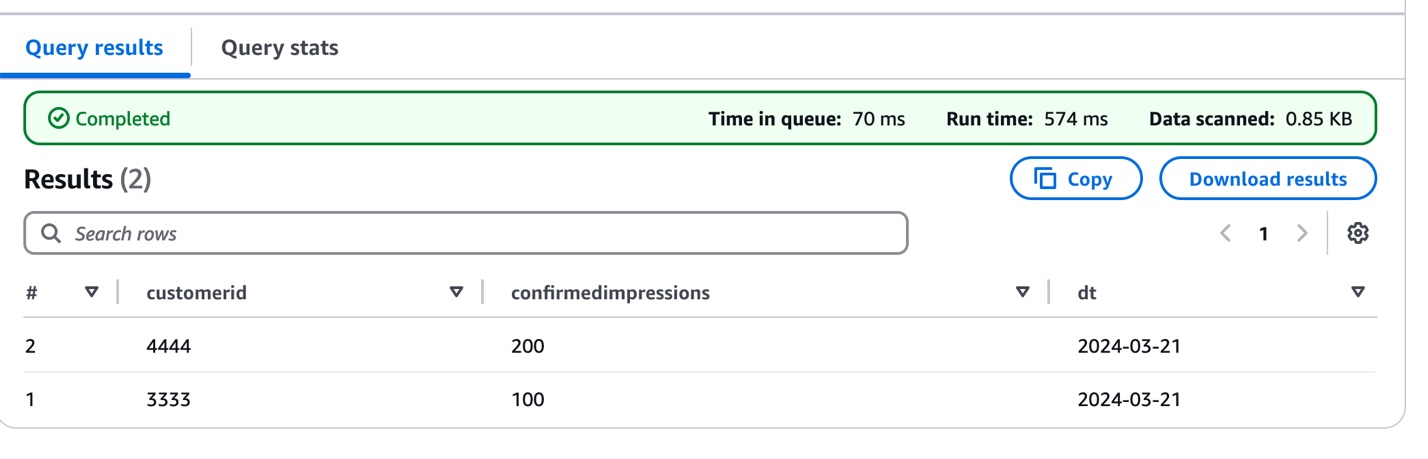
  1. Validate your sensor data ingestion by querying the newly loaded partition. This query helps verify that your sensor readings are correctly loaded and accessible:
SELECT * FROM "blogpostdatabase "."iot_sensor_data" WHERE dt='2024-03-21';

The following screenshot shows the query results.

This initial data load establishes the foundation for the IoT data pipeline, which means you can begin tracking sensor measurements while preparing for future schema evolution as sensor capabilities expand or change.

Now, we demonstrate how the IoT data pipeline handles evolving sensor capabilities by introducing a schema change in the second data batch. As sensors receive firmware updates or new monitoring features, their data structure needs to adapt accordingly. To show this evolution, we add data from sensors that now include visibility measurements:

  1. Examine the evolved schema structure that accommodates the new sensor capability:
{
  "fields": [
    {
      "Name": "customerid",
      "Type": "bigint",
      "Comment": "from deserializer"
    },
    {
      "Name": "sentiment",
      "Type": "struct<confirmedImpressions:bigint,visibility:bigint>",
      "Comment": "from deserializer"
    },
    {
      "Name": "dt",
      "Type": "string",
      "PartitionKey": "Partition (0)"
    }
  ]
}

Note the addition of the visibility field within the sentiment structure, representing the sensor’s enhanced monitoring capability.

  1. Upload this enhanced sensor data to a new date partition:
s3://amzn-s3-demo-bucket/dt=2024-03-22/
  1. Verify data consistency across both the original and enhanced sensor readings:
SELECT * FROM "blogpostdatabase"."blogpost_table_test" LIMIT 10;

This demonstrates how the pipeline can handle sensor upgrades while maintaining compatibility with historical data. In the next section, we explore how to update the table definition to properly manage this schema evolution, providing seamless querying across all sensor data regardless of when the sensors were upgraded. This approach is particularly valuable in IoT environments where sensor capabilities frequently evolve, which means you can maintain historical data while accommodating new monitoring features.

Update the AWS Glue table

To accommodate evolving sensor capabilities, you need to update the AWS Glue table schema. Although traditional methods such as MSCK REPAIR TABLE or ALTER TABLE ADD PARTITION work for small datasets for updating partition information, you can use an alternate method to handle tables with more than 100K partitions efficiently.

We use the Athena partition projection, which eliminates the need to process extensive partition metadata, which can be time-consuming for large datasets. Instead, it dynamically infers partition existence and location, allowing for more efficient data management. This method also speeds up query planning by quickly identifying relevant partitions, leading to faster query execution. Additionally, it reduces the number of API calls to the metadata store, potentially lowering costs associated with these operations. Perhaps most importantly, this solution maintains performance as the number of partitions grows, prodicing scalability for evolving datasets. These benefits combine to create a more efficient and cost-effective way of handling schema evolution in large-scale data environments.

To update your table schema to handle the new sensor data, follow these steps:

  1. Copy the following code into the UpdateTableAPI.py file:
import boto3

client = boto3.client('glue')

db = 'blogpostdatabase'
tb = 'blogpost_table_test'

response = client.get_table(
    DatabaseName=db,
    Name=tb
)

print(response)


table_input = {
    'Description': response['Table'].get('Description', ''),
    'Name': response['Table'].get('Name', ''),
    'Owner': response['Table'].get('Owner', ''),
    'Parameters': response['Table'].get('Parameters', {}),
    'PartitionKeys': response['Table'].get('PartitionKeys', []),
    'Retention': response['Table'].get('Retention'),
    'StorageDescriptor': response['Table'].get('StorageDescriptor', {}),
    'TableType': response['Table'].get('TableType', ''),
    'ViewExpandedText': response['Table'].get('ViewExpandedText', ''),
    'ViewOriginalText': response['Table'].get('ViewOriginalText', '')

}

for col in table_input['StorageDescriptor']['Columns']:
    if col['Name'] == 'sentiment':
        col['Type'] = 'struct<confirmedImpressions:bigint,visibility:bigint>'


table_input['StorageDescriptor']['SerdeInfo']['Parameters']['avro.schema.literal'] = '{"type" : "record", "name" : "customerdata", "namespace" : "com.data.test.avro", "fields" : [{ "name" : "customerID", "type" : "long", "default" : -1 },{ "name" : "sentiment", "type" : [ "null", { "type" : "record", "name" : "sentiment", "doc" : "***** CoreETL ******", "fields" : [ { "name" : "customerrating", "type" : "long", "default" : 0 },{"name":"visibility","type":"long","default":0}] } ], "default" : 0 }]}'
table_input['Parameters']['avro.schema.literal'] = '{"type" : "record", "name" : "customerdata", "namespace" : "com.data.test.avro", "fields" : [{ "name" : "customerID", "type" : "long", "default" : -1 },{ "name" : "sentiment", "type" : [ "null", { "type" : "record", "name" : "sentiment", "doc" : "***** CoreETL ******", "fields" : [ { "name" : "customerrating", "type" : "long", "default" : 0 },{"name":"visibility","type":"long","default":0} ] } ], "default" : 0 }]}'
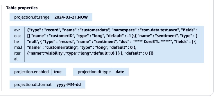
table_input['Parameters']['projection.dt.type'] = 'date'
table_input['Parameters']['projection.dt.format'] = 'yyyy-MM-dd'
table_input['Parameters']['projection.enabled'] = 'true'
table_input['Parameters']['projection.dt.range'] = '2024-03-21,NOW'

response = client.update_table(
    DatabaseName=db,
    TableInput=table_input
)

This Python script demonstrates how to update an AWS Glue table to accommodate schema evolution and enable partition projection:

  1. It uses Boto3 to interact with AWS Glue API.
  2. Retrieves the current table definition from the AWS Glue Data Catalog.
  3. Updates the 'sentiment' column structure to include new fields.
  4. Modifies the Avro schema literal to reflect the updated structure.
  5. Adds partition projection parameters for the partition column dt
    table_input['Parameters']['projection.dt.type'] = 'date'
    table_input['Parameters']['projection.dt.format'] = 'yyyy-MM-dd'
    table_input['Parameters']['projection.enabled'] = 'true'
    table_input['Parameters']['projection.dt.range'] = '2024-03-21,NOW'

    1. Sets projection type to 'date'
    2. Defines date format as 'yyyy-MM-dd'
    3. Enables partition projection
    4. Sets date range from '2024-03-21' to 'NOW'
projection.date.type='date' --> Data type of the partition column
projection.date.format='yyyy-MM-dd' -> Data format of the partition column
projection.enabled='true' -> Enable the partition projection
projection.date.range='2024-04-26,NOW'. -> The range of the partition column
  1. Run the script using the following command:
python3 UpdateTableAPI.py

The script applies all changes back to the AWS Glue table using the UpdateTable API call. The following screenshot shows the table property with the new Avro schema literal and the partition projection.

After the table property is updated, you don’t need to add the partitions manually using the MSCK REPAIR TABLE or ALTER TABLE command. You can validate the result by running the query in the Athena console.

SELECT * FROM "blogpostdatabase"." blogpost_table_test " limit 10;

The following screenshot shows the query results.

This schema evolution strategy efficiently handles new data fields across different time periods. Consider the 'visibility' field introduced on 2024-03-22. For data from 2024-03-21, where this field doesn’t exist, the solution automatically returns a default value of 0. This approach makes the query consistent across all partitions, regardless of their schema version.

Here’s the Avro schema configuration that enables this flexibility:

{
  "type": "record",
  "name": "customerdata",
  "fields": [
    {"name": "customerID", "type": "long", "default": -1},
    {"name": "sentiment", "type": ["null", {
      "type": "record",
      "name": "sentiment",
      "fields": [
        {"name": "customerrating", "type": "long", "default": 0},
        {"name": "visibility", "type": "long", "default": 0}
      ]
    }], "default": null}
  ]
}

Using this configuration, you can run queries across all partitions without modifications, maintain backward compatibility without data migration, and support gradual schema evolution without breaking existing queries.

Building on the schema evolution example, we now introduce a third enhancement to the sensor data structure. This new iteration adds a text-based classification capability through a 'category' field (string type) to the sentiment structure. This represents a real-world scenario where sensors receive updates that add new classification capabilities, requiring the data pipeline to handle both numeric measurements and textual categorizations.

The following is the enhanced schema structure:

{
  "fields": [
    {
      "Name": "customerid",
      "Type": "bigint"
    },
    {
      "Name": "sentiment",
      "Type": "struct<confirmedImpressions:bigint,visibility:bigint,category:string>"
    },
    {
      "Name": "dt",
      "Type": "string"
    }
  ]
}

This evolution demonstrates how the solution flexibly accommodates different data types as sensor capabilities expand while maintaining compatibility with historical data.

To implement this latest schema evolution for the new partition (dt=2024-03-23), we update the table definition to include the ‘category’ field. Here’s the modified UpdateTableAPI.py script that handles this change:

  1. Update the file UpdateTableAPI.py:
import boto3

client = boto3.client('glue')

db = 'blogpostdatabase'
tb = 'blogpost_table_test'

response = client.get_table(
DatabaseName=db,
Name=tb
)

print(response)


table_input = {
'Description': response['Table'].get('Description', ''),
'Name': response['Table'].get('Name', ''),
'Owner': response['Table'].get('Owner', ''),
'Parameters': response['Table'].get('Parameters', {}),
'PartitionKeys': response['Table'].get('PartitionKeys', []),
'Retention': response['Table'].get('Retention'),
'StorageDescriptor': response['Table'].get('StorageDescriptor', {}),
'TableType': response['Table'].get('TableType', ''),
'ViewExpandedText': response['Table'].get('ViewExpandedText', ''),
'ViewOriginalText': response['Table'].get('ViewOriginalText', '')

}

for col in table_input['StorageDescriptor']['Columns']:
if col['Name'] == 'sentiment':
col['Type'] = 'struct<confirmedImpressions:bigint,visibility:bigint,category:string>'


table_input['StorageDescriptor']['SerdeInfo']['Parameters']['avro.schema.literal'] = '{"type" : "record", "name" : "customerdata", "namespace" : "com.data.test.avro", "fields" : [{ "name" : "customerID", "type" : "long", "default" : -1 },{ "name" : "sentiment", "type" : [ "null", { "type" : "record", "name" : "sentiment", "doc" : "***** CoreETL ******", "fields" : [ { "name" : "customerrating", "type" : "long", "default" : 0 },{"name":"visibility","type":"long","default":0},{"name":"category","type":"string","default":"null"} ] } ], "default" : 0 }]}'
table_input['Parameters']['avro.schema.literal'] = '{"type" : "record", "name" : "customerdata", "namespace" : "com.data.test.avro", "fields" : [{ "name" : "customerID", "type" : "long", "default" : -1 },{ "name" : "sentiment", "type" : [ "null", { "type" : "record", "name" : "sentiment", "doc" : "***** CoreETL ******", "fields" : [ { "name" : "customerrating", "type" : "long", "default" : 0 },{"name":"visibility","type":"long","default":0},{"name":"category","type":"string","default":"null"} ] } ], "default" : 0 }]}'
table_input['Parameters']['projection.dt.type'] = 'date'
table_input['Parameters']['projection.dt.format'] = 'yyyy-MM-dd'
table_input['Parameters']['projection.enabled'] = 'true'
table_input['Parameters']['projection.dt.range'] = '2024-03-21,NOW'

response = client.update_table(
DatabaseName=db,
TableInput=table_input
)
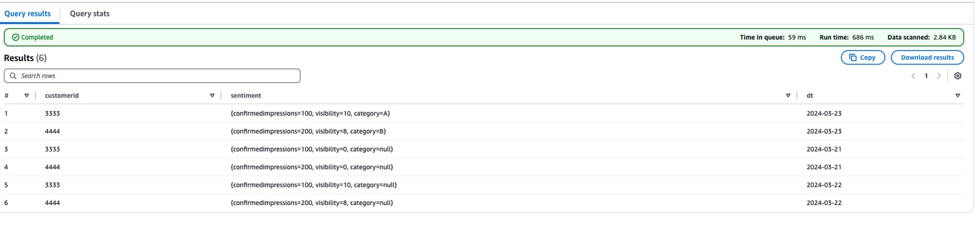
  1. Verify the changes by running the following query:
SELECT * FROM "blogpostdatabase"."blogpost_table_test" LIMIT 10;

The following screenshot shows the query results.

There are three key changes in this update:

  1. Added 'category' field (string type) to the sentiment structure
  2. Set default value "null" for the category field
  3. Maintained existing partition projection settings

To support that latest sensor data enhancement, we updated the table definition to include a new text-based 'category' field in the sentiment structure. The modified UpdateTableAPI script adds this capability while maintaining the established schema evolution patterns. It achieves this by updating both the AWS Glue table schema and the Avro schema literal, setting a default value of "null" for the category field.

This provides backward compatibility. Older data (before 2024-03-23) shows "null" for the category field, and new data includes actual category values. The script maintains the partition projection settings, enabling efficient querying across all time periods.

You can verify this update by querying the table in Athena, which will now show the complete data structure, including numeric measurements (customerrating, visibility) and text categorization (category) across all partitions. This enhancement demonstrates how the solution can seamlessly incorporate different data types while preserving historical data integrity and query performance.

Cleanup

To avoid incurring future costs, delete your Amazon S3 data if you no longer need it.

Conclusion

By combining Avro’s schema evolution capabilities with the power of AWS Glue APIs, we’ve created a robust framework for managing diverse, evolving datasets. This approach not only simplifies data integration but also enhances the agility and effectiveness of your analytics pipeline, paving the way for more sophisticated predictive and prescriptive analytics.

This solution offers several key advantages. It’s flexible, adapting to changing data structures without disrupting existing analytics processes. It’s scalable, able to handle growing volumes of data and evolving schemas efficiently. You can automate it and reduce the manual overhead in schema management and updates. Finally, because it minimizes data movement and transformation costs, it’s cost-effective.

Related references


About the authors

Mohammad Sabeel Mohammad Sabeel is a Senior Cloud Support Engineer at Amazon Web Services (AWS) with over 14 years of experience in Information Technology (IT). As a member of the Technical Field Community (TFC) Analytics team, he is a Subject matter expert in Analytics services AWS Glue, Amazon Managed Workflows for Apache Airflow (MWAA), and Amazon Athena services. Sabeel provides expert guidance and technical support to enterprise and strategic customers, helping them optimize their data analytics solutions and overcome complex challenges. With deep subject matter expertise he enables organizations to build scalable, efficient, and cost-effective data processing pipelines.

Indira Balakrishnan Indira Balakrishnan is a Principal Solutions Architect in the Amazon Web Services (AWS) Analytics Specialist Solutions Architect (SA) Team. She helps customers build cloud-based Data and AI/ML solutions to address business challenges. With over 25 years of experience in Information Technology (IT), Indira actively contributes to the AWS Analytics Technical Field community, supporting customers across various Domains and Industries. Indira participates in Women in Engineering and Women at Amazon tech groups to encourage girls to pursue STEM path to enter careers in IT. She also volunteers in early career mentoring circles.
New AWS whitepaper: AWS User Guide to Financial Services Regulations and Guidelines in Australia

Post Syndicated from Julian Busic original https://aws.amazon.com/blogs/security/new-aws-whitepaper-aws-user-guide-to-financial-services-regulations-and-guidelines-in-australia/

Amazon Web Services (AWS) has released substantial updates to its AWS User Guide to Financial Services Regulations and Guidelines in Australia to help financial services customers in Australia accelerate their use of AWS.

The updates reflect the Australian Prudential Regulation Authority’s (APRA) publication of the Prudential Standard CPS 230 Operational Risk Management (CPS 230), which became effective from July 1, 2025. It also reflects that APRA rescinded its 2018 information paper “Outsourcing Involving Cloud Computing Services” in February 2025.

The updated whitepaper continues our efforts to help AWS customers navigate APRA’s regulatory expectations in a shared responsibility environment. It is intended for APRA-regulated institutions that are looking to run workloads on AWS and is particularly useful for leadership, governance, security, risk, and compliance teams that need to understand APRA requirements and guidance.

The whitepaper summarizes APRA’s requirements and guidance related to operational risk management and information security. It also gives APRA-regulated institutions information they can use to commence their due diligence and assess how to implement the appropriate programs for their use of AWS.

As the regulatory environment continues to evolve, we’ll provide further updates through the AWS Security Blog and the AWS Compliance page. You can find more information on cloud-related regulatory compliance at the AWS Compliance Center. You can also reach out to your AWS account manager for help finding the resources you need.

If you have feedback about this post, submit comments in the Comments section below. If you have questions about this post, contact AWS Support.

Julian Busic
Julian Busic

Julian is a Security Solutions Architect for AWS with a focus on regulatory engagement. He works with our customers, their regulators, and AWS teams to help customers raise the bar on secure cloud adoption and usage. Julian has over 15 years of experience working in risk and technology across the financial services industry in Australia and New Zealand.
Krish De
Krish De

Krish is a Principal FSI Governance, Risk & Compliance (GRC) specialist. He works with AWS customers, their regulators, and AWS teams to safely accelerate customers’ cloud adoption by providing prescriptive guidance on GRC. Krish has over 20 years of experience working in governance, risk, and technology across the financial services industry in Australia, New Zealand, and the United States.
Paul Curtis
Paul Curtis

Paul is a Principal FSI Risk & Compliance Specialist. He works with AWS financial services customers assisting them in navigating the regulatory environment while transforming their risk and controls management through the transparency and potential for automation that AWS makes available. Paul has over 20 years of experience working in risk and technology across APAC.
Katherine Velos
Katherine Velos

Katherine is the lead legal counsel for AWS Financial Services in ANZ and has supported AWS Sales and Marketing teams in EMEA and Asia-Pacific.

AWS Security Incident Response: The customer’s journey to accelerating the incident response lifecycle

Post Syndicated from Jason Hurst original https://aws.amazon.com/blogs/security/aws-security-incident-response-the-customers-journey-to-accelerating-the-incident-response-lifecycle/

Organizations face mounting challenges in building and maintaining effective security incident response programs. Studies from IBM and Morning Consult show security teams face two major challenges: over 50 percent of security alerts go unaddressed because of resource constraints and alert fatigue, while false positives consume 30 percent of investigation time, delaying responses to true positive threats

According to the 2024 IBM Cost of a Data Breach Report, organizations now take an average of 258 days to identify and contain security events. The report also reveals that nearly half of SOC teams report increased detection and response times over the past two years, with 80 percent indicating that manual threat investigation significantly impacts their response times.

Despite these challenges, according to the 2024 IBM Security Services Benchmark Report, organizations with mature incident response capabilities demonstrate a 50 percent reduction in mean time to resolution (MTTR) and achieve cost savings of up to 58 percent per incident. These improvements are driven by the adoption of automated workflows, integrated tools, and streamlined communication processes that accelerate threat detection and containment.

In this post, we walk you through a real-world scenario to show how AWS Security Incident Response can immediately generate benefits by accelerating every step of your incident response lifecycle, how it integrates with other native AWS services such as Amazon GuardDuty, AWS Security Hub, and AWS Systems Manager, and how to integrate third-party threat detection findings for inclusion in your automated monitoring, triage, and containment capabilities.

How AWS Security Incident Response can help

AWS Security Incident Response is a Tier 1 service that launched in December 2024. The service is an AWS-native, purpose-built security incident response solution for customers that can be used as a better-together experience with other AWS services in the areas of detection and response (GuardDuty and Security Hub), networking and content delivery (AWS WAF and AWS Shield), and management and governance (Systems Manager). AWS Security Incident Response is also integrated across AWS Partners through a service specific Partner Specialization program. More detailed information is available in the AWS Security Incident Response documentation.

AWS Security Incident Response complements existing services by enhancing your security posture through streamlined incident management capabilities before, during, and after security events.

Key challenges

AWS Security Incident Response addresses three common challenges:

  • Alert fatigue: It can reduce alert fatigue and accelerate security investigations through automated monitoring and intelligent triage, reducing false positives and helping to prevent security team burnout.
  • Fragmented access and communications: By simplifying AWS Management Console permissions management and unifying incident response team communications, it can resolve fragmented access issues.
  • Security skills gaps: It can bridge cloud security skills gaps by providing 24/7 access to AWS security experts who support the incidents including credential compromise, data exfiltration, and ransomware. The AWS Security Incident Response service allows security teams to handle immediate security challenges while maintaining focus on strategic long-term preparedness and operational improvements.

Service integration

AWS Security Incident Response complements and integrates with AWS security services to provide comprehensive incident response capabilities. The service works seamlessly with:

This integration helps you build efficient incident response capabilities that can minimize the time, cost, and impact of security events throughout your organization’s cloud journey, while helping to reduce investments in additional staffing, training, and tool maintenance.

Distinct capabilities

The AWS Security Incident Response service offers:

  • Expert knowledge from the AWS Customer Incident Response Team (CIRT)
  • Tools through APIs and the console
  • Streamlined processes for handling security incidents

Prerequisites

Before implementing the capabilities described in this post, make sure that you have:

  • Configured the appropriate AWS Identity and Access Management (IAM) permissions
  • Established incident response team contacts
  • Set up notification channels
  • (OPTIONAL) Enabled GuardDuty in your accounts and AWS Regions
  • (OPTIONAL) Enabled SecurityHub in your accounts and Regions
  • (OPTIONAL) Deployed the required AWS CloudFormation StackSets for automated actions

These prerequisites help make sure that you can fully utilize the service’s automated detection, triage, and response capabilities.

The service provides automated monitoring and analysis capabilities within its own service infrastructure, enabling automatic triage of findings from GuardDuty and Security Hub.

For automated containment actions in your AWS accounts, you must first deploy the required CloudFormation StackSets and configure the appropriate IAM permissions. This helps make sure that you maintain full control over automated actions taken in your environment while benefiting from the service’s detection capabilities. This automation can be customized based on variables you establish, such as known CIDR ranges (specific ranges of IP addresses that define your network) and IP addresses, and you can implement GuardDuty suppression rules to help reduce false positives and alert volumes. As a result, the service can serve as a powerful augmentation to your existing security incident response programs and tools.

Setting up AWS Security Incident Response

Your cloud administrator, with AWSSecurityIncidentResponseFullAccess permissions, has established the incident response team in the service. The service notifies individuals, your partners or managed security service provider (MSSP), and other contacts added to the team, supporting a rapid escalation to alert the required parties and respond to the event.

As a best practice, your team establishes minimal privileges for accessing and managing information within AWS Security Incident Response cases. This helps make sure that team members have appropriate access levels to case details, findings, and investigation data while maintaining security and compliance requirements. AWS Security Incident Response provides multiple API actions, such as CreateCaseComment (to add notes to investigations) and GetCase (to retrieve case metadata), to limit whom and which actions can be performed against differing cases. For development and testing environments, AWS provides role-based policies that you can use such as AWSSecurityIncidentResponseCaseFullAccess and AWSSecurityIncidentResponseReadOnlyAccess for role-based access control (as shown in Figure 1). For production environments, we recommend creating custom IAM policies following the principle of least privilege based on your security requirements.

Figure 1: Permissions policies for security incident response

Figure 1: Permissions policies for security incident response

Following your configuration of the AWS Security Incident Response service, your security team reviews the email distribution list or alias for notifications for notifications from the service, as shown in Figure 2. You have developed items in your backlog to take advantage of Amazon EventBridge integrations to add in pager duty, Jira, and other services in the future for additional notification mechanisms.

Figure 2: Use the console to manage your incident response team membership

Figure 2: Use the console to manage your incident response team membership

Detecting and responding to suspicious activity

At 2:00 AM, days after AWS Security Incident Response has been set up, the service detects a combination of suspicious activities through GuardDuty findings, including anomalous IAM user behavior (such as shown in Figure 3), unusual API calls from unknown IP addresses, and a surge of Amazon Elastic Compute Cloud (Amazon EC2) instance creations that deviate from your account’s normal baseline. This pattern of activities matches known threat behaviors monitored by GuardDuty Extended Threat Detection. Without the service, security teams would need to manually analyze and correlate these separate findings across accounts and Regions. Instead, the service automatically identifies the pattern of suspicious activities.

Figure 3: Pattern of potentially suspicious activity

Figure 3: Pattern of potentially suspicious activity

One of the anomalous behaviors is a surge of unrecognized EC2 instance creations, complete with SSH keys (secure credentials used for remote access) and security group configurations (firewall rules that control network traffic) allowing internet connectivity. Using this example scenario, let’s walk through how the service’s automated monitoring, triage and containment capabilities, access management, API actions for custom integrations, collaboration tools, and 24/7 AWS security experts work together to help you navigate security incident response challenges across your AWS environment.

Incident Response Timeline
    dateFormat HH:mm
    axisFormat %H:%M
    
    section Detection
    GuardDuty Alerts          :02:00, 15m
    Automated Analysis        :after Detection, 10m
    
    section Investigation
    Case Creation             :02:25, 5m
    Team Notification         :02:30, 5m
    Initial Assessment        :02:35, 25m
    
    section Response
    AWS CIRT Engagement       :03:00, 30m
    Resource Tagging          :03:30, 15m
    Containment Actions       :03:45, 30m
    
    section Resolution
    Threat Elimination        :04:15, 30m
    Service Restoration       :04:45, 45m
    Documentation             :05:30, 30m

With the initial detection complete, the next phase focuses on centralizing and analyzing the security findings to understand the full scope of the incident.

Centralizing security findings: A systematic approach

GuardDuty begins to generate findings in your enabled Regions.

Note: GuardDuty must be enabled in your accounts and Regions. For setup instructions, see the GuardDuty documentation.

Because AWS Security Incident Response is integrated with GuardDuty, these findings are automatically sent to the service for internal processing, analysis, and auto-triage without manual effort. The service’s proactive response and alert triaging feature analyzes multiple factors, including your account’s historical baseline activity, specific GuardDuty finding types, and correlation patterns across accounts. In this case, it identified anomalous EC2 instance creation activity that deviated significantly from your environment’s normal patterns.

When the service identifies a true positive, an AWS Security Incident Response case is opened automatically (see Figure 4), resulting in a notification to the incident response team you configured earlier. A central benefit is how the service correlates disparate events—connecting the instance creations with the security group modifications—to paint a complete picture of the potential security event.

Figure 4: Automated incident remediation flow

Figure 4: Automated incident remediation flow

This proactive monitoring and analysis, as documented in your monthly service reports, demonstrates tangible benefits by reducing alert fatigue, and providing intelligent triage capabilities to SOC teams every day. The service’s automated analysis and correlation capabilities set the stage for rapid response when security events occur, which means that your team can focus on strategic security initiatives instead of spending time manually investigating alerts. The service feature helps you maintain strong security in two ways:

  • Comprehensive monitoring across configured Regions.
  • Integration with third-party security tools. This automated approach reduces the time, cost, and impact of security events.

As the investigation progresses from initial detection to detailed analysis, the GuardDuty integration provides crucial insights into the threat patterns.

From detection to action: The GuardDuty integration story

As your security team responds to the internal detection mechanisms, AWS Security Incident Response processes security findings in three key steps:

  • It analyzes GuardDuty alerts to identify genuine security threats
  • Using GuardDuty Extended Threat Detection, it correlates related events to identify threat patterns
  • It tracks the threat sequence, from initial actions (deleting logs or creating unauthorized access) through to potential data theft attempts

For this event, the sequence started with the deletion of CloudTrail logs, followed by the creation of unauthorized access keys. As the threat progressed, the service identified suspicious Amazon Simple Storage Service (Amazon S3) object access patterns and potential data exfiltration attempts, along with sophisticated evasion techniques and persistence mechanisms. Each of these signals maps directly to specific MITRE ATT&CK® tactics, techniques and procedures (TTPs), revealing the systematic nature of a potential ransomware threat. For detailed mapping of AWS Security Incident Response findings to MITRE ATT&CK® frameworks, see Mapping AWS security services to MITRE frameworks for threat detection and mitigation.

The service assists in correlation and analysis, evaluating patterns such as deletion of CloudTrail trails, creation of new access keys, and suspicious actions targeting S3 objects. When the AI and machine learning (AI/ML) capabilities of GuardDuty detect these concerning patterns over periods of time, the service automatically elevates the situation by creating an AWS Security Incident Response case on your behalf, bringing additional resources and focused attention to the situation. The incident response team defined in the earlier steps are then notified by email or other methods (shown in Figure 5) that a new triaged event has been created and to begin their investigations. 

The benefits include the service coordinating communication across your affected accounts. Instead of juggling multiple alerts and trying to piece together the scope of the potential ransomware incident, GuardDuty Extended Threat Detection provides a comprehensive view of the threat sequence, while the AWS Security Incident Response case offers a single, coherent channel for triaging these signals and providing coordination as your global team comes online to join the response effort.

Figure 5: Incident alert message

Figure 5: Incident alert message

Additional examples and further information are available in Introducing Amazon GuardDuty Extended Threat Detection: AI/ML attack sequence identification for enhanced cloud security.

Note: For brevity, Security Hub’s workflow details have been omitted because they mirror the monitoring and escalation processes described above for GuardDuty. Both services integrate closely and share similar operational patterns, with GuardDuty findings being sent to Security Hub within five minutes of detection. Security Hub enhances security coverage by aggregating findings from multiple AWS services and third-party partners.

With the threat patterns identified, your team moves to the next phase—engaging AWS CIRT for specialized expertise and advanced investigation capabilities.

Partnering with AWS CIRT through the incident response case

Your team continues investigating the event and discovers that they need additional assistance. An authorized user in your account opens a service supported case to request assistance from AWS. 

The AWS Security Incident Response case establishes a direct communication channel with AWS CIRT (shown in Figure 6) with a one-click escalation of the case within the console, providing immediate access to specialized expertise. Upon case escalation, AWS CIRT engages through the incident response case with a 15-minute acknowledgement timeframe, bringing their advanced tooling and specialized knowledge to analyze patterns across your accounts—even in environments with limited logging capabilities. This partnership delivers:

  • Real-time collaboration through conference bridge video calls
  • Advanced artifact analysis and pattern recognition
  • Technical guidance for investigation and containment
  • Recommendations for improving security posture
Figure 6: Connect with the AWS CIRT

Figure 6: Connect with the AWS CIRT

Figure 6 is an example of how this would appear in your account, with the resolver set to Self for a self-managed case.

Returning to the scenario, you discover that multiple accounts have insufficient logging enabled—which limits the available investigation data. While AWS CIRT can provide additional insights through specialized tooling, maintaining comprehensive logging across your accounts remains crucial for security visibility, compliance requirements, and thorough incident investigations. The capabilities of AWS CIRT complement—but do not replace—proper logging practices. This capability provides an understanding of the scope of the incident, as they see patterns and activities otherwise invisible to you.

The collaboration begins with AWS CIRT analyzing your environment using their tooling, looking for anomalous patterns beyond what you see in your immediate logs. Through the incident response case, they help you understand the scope of your situation by:

  • Communicating their findings
  • Recommending additional investigation paths
  • Sharing analysis showing similar EC2 instance creation patterns from other environments

AWS CIRT uses the incident response case to establish a bridge call, bringing together their team and yours for real-time collaboration. During these calls, AWS CIRT shares their ongoing analysis of artifacts and service data, helping you understand what happened, why it happened, and how to prevent similar issues in the future. They also provide guidance on implementing proper logging across your accounts to improve your future security posture.

Managing the incident through intelligent tagging

As AWS CIRT begins their analysis, your team implements real-time resource tagging using the incident case ID. This systematic tagging approach proves crucial for tracking and managing the suspicious EC2 instances across your accounts. By using tags, you can quickly implement isolation policies and track costs while maintaining clear documentation of affected resources throughout the investigation. 

Your tag-based approach helps track affected resources to implement isolation policies. You used the incident case ID tags to quickly identify resources connected to the incident, which you use to apply targeted access controls and containment measures. The tags also help you track costs associated with the incident, giving your finance team precise visibility into the event’s financial impact.

Working alongside the AWS Security Incident Response service, you find that using the incident case ID as your primary tag key (shown in Figure 7) created a consistent way to correlate resources across affected accounts. This proves especially helpful when coordinating with AWS CIRT, because you can quickly direct them to specific resources requiring investigation. Even after containment, these tags continue to provide value in supporting your post-incident analysis and helping you implement targeted security controls based on what you learn from the incident.

Figure 7: Incident tags

Figure 7: Incident tags

Automated containment options through Systems Manager integration

While working with AWS CIRT to understand the incident scope, you can also use Systems Manager to help automatically contain threats. Your team previously deployed the required CloudFormation StackSets across your organization, enabling Amazon EC2 containment actions through Systems Manager.

The setup process required deploying CloudFormation StackSets with specific IAM roles and Systems Manager configurations across your accounts. This infrastructure allows the AWS Security Incident Response service to make containment actions on your behalf. These actions can be reversed if needed—similar to using an undo function—so that you can restore systems to their previous state.

When authorized through your pre-deployed CloudFormation StackSets, AWS Security Incident Response service can request Systems Manager to implement containment measures. Containment actions require explicit customer authorization and proper IAM permissions to be configured in advance. The service isolates the tagged suspicious instances by modifying their security groups and network access, while preserving their state to maintain forensic integrity for analysis. 

The containment process happens in three steps:

  1. Isolate: Remove compromised instances from security groups
  2. Preserve: Create backup copies (snapshots) of affected systems
  3. Investigate: Collect system information using Systems Manager

These actions can be reversed if needed, supporting containment decisions for legitimate workloads.

The automation capabilities help streamline containment procedures across multiple instances, reducing the time taken to contain impacted resources. The service maintains detailed logs of each action in the incident response case, providing your team with clear visibility into the containment efforts.

Through this response capability, combined with the guidance from AWS CIRT, you can contain the incident’s spread within minutes rather than hours. The Systems Manager integration provides a reliable way to implement containment actions while preserving evidence for investigation (shown in Figure 8).

Figure 8: Systems Manager documents for containment actions

Figure 8: Systems Manager documents for containment actions

Resolution and lessons learned

As the incident moves toward resolution, your team works through a systematic process to verify containment, alleviate threats, and restore services. Working alongside AWS CIRT through the AWS Security Incident Response case, you implement a structured approach to make sure that affected resources are secured and normal operations can safely resume. The immediate resolution actions fall into three main categories:

  • Containment confirmation through Systems Manager verification
    • Verify security group modifications are in place
    • Confirm network isolation of affected instances
    • Validate that automated containment actions were successful
    • Review Systems Manager logs for containment action completion
  • Verification of threat alleviation across affected resources
    • Analyze GuardDuty findings to confirm that there’s no new suspicious activity
    • Review tagged resources for complete containment
    • Verify termination of unauthorized access attempts
    • Confirm removal of persistence mechanisms
    • Check for remaining unauthorized IAM access
  • Service restoration and access control normalization
    • Restore legitimate workload access based on verified baselines
    • Implement updated security group configurations
    • Reset affected IAM credentials and access keys
    • Re-establish normal network connectivity for verified clean resources
    • Update resource tags to reflect post-incident status

Documentation and reporting:

As the incident reaches resolution, AWS Security Incident Response service compiles a comprehensive incident timeline. This documentation accelerates your reporting process, helping you quickly generate required reports for executives, regulators, and cyber insurance providers—all from within the incident response case.

The incident response case captures the complete timeline of events, starting with GuardDuty Extended Threat Detection identifying the initial threat sequences. Each step of the incident response is documented, from the moment suspicious EC2 instance creations were detected, through the MITRE ATT&CK® tactics observed, to the containment actions implemented through Systems Manager integration, and finally to the resolution steps that proved effective.

Long-term Improvements: Through this collaborative post-incident review process, your team:

  • Implements enhanced logging based on AWS CIRT recommendations
  • Updates security controls to help prevent similar incidents
  • Improves incident response processes based on lessons learned
  • Strengthens your security posture through targeted improvements

Conclusion

This example illustrates how AWS Security Incident Response service can enhance security operations through automated detection, triage, containment, access, and coordinated response capabilities. The service’s integration with AWS Security Hub and Amazon GuardDuty provides efficient handling of security events, while the optional escalation to the AWS CIRT can provide valuable expertise and specialized tooling to help accelerate every stage of your incident response lifecycle and strengthen your security posture.

AWS Security Incident Response service serves as a critical component of a comprehensive security operations strategy, delivering measurable benefits through:

  • Continuous threat monitoring for automated correlation and machine learning to identify high-priority security risks while minimizing false positives.
  • Reduced incident response times through automated detection and coordinated response
  • Enhanced investigation capabilities through direct AWS CIRT collaboration
  • Streamlined, rapid containment
  • Comprehensive incident documentation and audit trails to support and accelerate reporting requirements
  • Cost savings of up to 58 percent per incident

To prepare for, respond to and recover from security incidents faster and more efficiently today, visit AWS Security Incident Response or contact your AWS account team to schedule a discussion.

Additional resources

Here are some additional AWS resources that your teams can use to further improve your security incident response capabilities: 

Before an event:

  • AWS Customer Playbook Framework: Publicly available response frameworks that use AWS CIRT lessons learned from security events
  • Assisted Log Enabler: A tool that assists customers to enable logs, including the following: Amazon VPC Flow Logs, AWS CloudTrail, Amazon Elastic Kubernetes Service audit and authenticator logs, Amazon Route 53 Resolver Query Logs, Amazon S3 server access logs, and Elastic Load Balancing logs

During an event:

  • Athena Security Analytics Bootstrap: A tool for customers who need a quick method to set up Amazon Athena and perform investigations on AWS service logs archived in S3 buckets

Before or following an event:

Jason Hurst

Jason Hurst

Jason is a Senior Incident Responder and the Knowledge Manager for AWS CIRT. He is passionate about developing others, teaching part-time at a local technical college. Jason has three dogs that entertain him in his spare time.

Christopher Rae

Christopher Rae

Christopher is a Principal Worldwide Security Specialist at AWS, where he drives worldwide business development strategy and implementation to accelerate and scale adoption of AWS security solutions. He is passionate about the intersection of cybersecurity and emerging technologies, with 20+ years of experience in strategic leadership roles delivering security products and services to media, entertainment, and telecommunications customers globally.

Nooms Charania

Nooms Charania

Nooms is a Sr. PMT – ES at AWS Global Services Security, with an MBA from Yale and engineering background from USC. He specializes in technical product management and previously interned with AWS during his MBA program.

New whitepaper available: AICPA SOC 2 Compliance Guide on AWS

Post Syndicated from Abdul Javid original https://aws.amazon.com/blogs/security/new-whitepaper-available-aicpa-soc-2-compliance-guide-on-aws/

We’re excited to announce the release of our latest whitepaper, AICPA SOC 2 Compliance Guide on AWS, which provides in-depth guidance on implementing and maintaining SOC 2-aligned controls using AWS services.

Building and operating cloud-native services in alignment with the AICPA’s Trust Services Criteria requires thoughtful planning and robust implementation. This new whitepaper helps cloud architects, security and compliance teams, and DevOps professionals design environments that meet SOC 2 requirements while leveraging AWS’s shared responsibility model.

What’s inside the whitepaper:

  • Overview of the SOC 2 framework—including Common Criteria (CC 1–CC 9) and category-specific criteria (Security, Availability, Processing Integrity, Confidentiality, Privacy)
  • Mapping of each Trust Services Criterion to AWS services and constructs
  • Guidance on implementing complementary user entity controls (CUECs)
  • Strategies for evidence collection, documentation, and audit procedures
  • Risk and governance for executives
  • Best practices for automating compliance and preparing for SOC 2 readiness assessments

Download AICPA SOC 2 Compliance Guide on AWS.

For further assistance, contact AWS Security Assurance Services.

If you have feedback about this post, submit comments in the Comments section below.

Abdul Javid

Abdul Javid

Abdul is a Senior Security Assurance Consultant and PCI DSS Qualified Security Assessor with AWS Security Assurance Services, and has more than 25 years of IT Governance, Operations, Security, Risk and Compliance. Abdul leverages his experience and knowledge to advise AWS customers with guidance and advisory on their compliance journey. Abdul earned a M.S in Computer Science from IIT, Chicago and holds various industry recognized sought after certifications in security, program & risk management from prominent organizations like AWS, HITRUST, ISACA, PMI, PCI DSS, ISC2.

Viktor Mu

Viktor Mu

Viktor is a Senior Assurance Consultant with AWS Security Assurance Services and has more than a decade of experience specializing in security and compliance assessments. In addition to technical certifications from AWS, Viktor holds several industry recognized audit and security certifications, including PCI QSA, CISA, etc. In his current role, Viktor is focusing on helping partners and customers understand the opportunities for cloud technology to handle security and compliance frameworks like SOC 2 in key market verticals and regulated industries.

Wil Woodrum

Wil Woodrum

Wil is a Senior Assurance Consultant with AWS Security Assurance Services. He has more than 20 years of experience in leading the development and implementation of effective systems of control for enterprise IT operations and assessing compliance with multiple frameworks, including SOC 2, PCI, NIST 800-53, and FedRAMP. Wil earned a Master of Business Administration from the Pennsylvania State University and maintains the following certifications: CISSP, CRISC, PCI QSA, CISA, AWS SAA, and ITIL. In his current role, Wil has specialized in assisting AWS customers to achieve compliance with NIST 800-53, FedRAMP, StateRAMP, and SOC 2 control frameworks.

Beyond IAM access keys: Modern authentication approaches for AWS

Post Syndicated from Mitch Beaumont original https://aws.amazon.com/blogs/security/beyond-iam-access-keys-modern-authentication-approaches-for-aws/

When it comes to AWS authentication, relying on long-term credentials, such as AWS Identity and Access Management (IAM) access keys, introduces unnecessary risks; including potential credential exposure, unauthorized sharing, or theft. In this post, I present five common use cases where AWS customers traditionally use IAM access keys and present more secure alternatives that you should consider.

AWS CLI access: Embrace CloudShell

If you’re primarily using access keys for AWS Command Line Interface (AWS CLI) access, consider AWS CloudShell—a browser-based CLI that minimizes the need for local credential management while providing the same powerful CLI capabilities that you’re accustomed to.

AWS CLI with enhanced security: IAM Identity Center

If you need a more robust solution, AWS CLI v2 combined with AWS IAM Identity Center offers a superior authentication approach. This integration enables:

  • Centralized user management
  • Seamless multi-factor authentication (MFA) integration
  • Enhanced security controls

Configuration is straightforward using the AWS CLI documentation, and MFA can be enabled following the IAM Identity Center MFA guide.

Local development: IDE integration

For developers working in local environments, modern integrated development environments (IDEs) such as Visual Studio Code, with AWS Toolkit support offer secure authentication through IAM Identity Center. This alleviates the need for static access keys while maintaining a smooth development experience. Learn more about AWS IDE integrations.

AWS compute services and CI/CD access

When your applications and automation pipelines need AWS resource access, whether running on AWS compute services (Amazon Elastic Compute Cloud (Amazon EC2), Amazon Elastic Container Service (Amazon ECS), or AWS Lambda) or through continuous integration and delivery (CI/CD) tools, IAM roles can provide the ideal solution. These roles automatically manage temporary credential rotation and follow security best practices.

  • For AWS compute services: Use standard IAM roles with your compute resources. Review the EC2 IAM roles documentation for implementation details.
  • For AWS-hosted CI/CD: When using AWS CodePipeline or AWS CodeBuild for example, use service-linked roles to manage permissions securely.
  • For CI/CD tools self-hosted on Amazon EC2: If you’re running tools such as Jenkins or GitLab on AWS resources, use the instance profile roles the same as you would with other compute services.

For third-party CI/CD services (such as GitHub Actions, CircleCI, and so on), see External access requirements.

External access requirements

For scenarios involving third-party applications or on-premises workloads, AWS offers three methods:

  • Third-party applications: Implement temporary security credentials through IAM roles instead of static access keys. Never use root account access keys. See third-party access documentation.
  • On-premises workloads: Use AWS IAM Roles Anywhere to generate temporary credentials for non-AWS workloads. For more information, see Access for non AWS workloads.
  • CI/CD software as a service (SaaS): For cloud-based CI/CD services, use OpenID Connect (OIDC) integration with IAM roles to minimize the need for long-term credentials. This allows your CI/CD pipelines to obtain temporary credentials through trust relationships. See the AWS OIDC provider documentation for implementation details.

Best practice: Principle of least privilege

Regardless of your authentication method, always implement the principle of least privilege. This helps make sure that users and applications have only the permissions they need. For guidance on crafting precise IAM policies, see Techniques for writing least privilege IAM policies.

Note: AWS also offers policy generation based on AWS CloudTrail logs, helping you create permission templates based on actual usage patterns. Learn about this feature in the IAM policy generation documentation.

Conclusion

As you’ve seen, there are numerous secure alternatives to IAM access keys that you can use to enhance your AWS authentication strategy while reducing security risks. By using tools such as CloudShell, IAM Identity Center, IDE integrations, IAM roles, and IAM Roles Anywhere, you can implement robust authentication mechanisms that align with modern security best practices.Key takeaways:

  • Prefer temporary credentials over long-term access keys
  • Choose the authentication method that best fits your use case
  • Implement the principle of least privilege across all access methods
  • Take advantage of the built-in tools provided by AWS for policy generation and management
  • Regularly review and update your authentication methods as new solutions become available

By making these changes, you can not only improve your security posture but also streamline your authentication processes across your AWS environment. Start small by identifying your current IAM access key use cases and gradually transition to these more secure alternatives. Your future self—and your security team—will thank you.

If you have feedback about this post, submit comments in the Comments section below.

Mitch Beaumont

Mitch Beaumont

Mitch is a Principal Solutions Architect for Amazon Web Services based in Sydney, Australia. Mitch works with some of Australia’s largest financial services customers, helping them to continually raise the security bar for the products and features that they build and ship. Outside of work, Mitch enjoys spending time with his family, photography, and surfing.

Building resilient multi-tenant systems with Amazon SQS fair queues

Post Syndicated from Maximilian Schellhorn original https://aws.amazon.com/blogs/compute/building-resilient-multi-tenant-systems-with-amazon-sqs-fair-queues/

Today, AWS introduced Amazon Simple Queue Service (Amazon SQS) fair queues, a new feature that mitigates noisy neighbor impact in multi-tenant systems. With fair queues, your applications become more resilient and easier to operate, reducing operational overhead while improving quality of service for your customers.

In distributed architectures, message queues have become the backbone of resilient system design. They act as buffers between components, allowing services to process work asynchronously and at their own pace. When a sudden traffic spike hits your application, queues prevent cascading failures by buffering work and ensuring that downstream services aren’t overwhelmed. Amazon SQS has long been a go-to solution for developers building scalable applications because it’s a fully managed serverless solution that can seamlessly scale to ingest millions of messages per second.

In this post, you learn how to use Amazon SQS fair queues and understand their inner workings through a practical example.

Overview

Many modern applications follow a multi-tenant architecture, where a single application instance serves multiple tenants. A tenant is any entity that shares resources with others. It could be a customer, client application, or request type. This approach reduces operational costs and simplifies maintenance through efficient resource utilization. One example of such shared resources are queues and their associated consumer capacity.

However, multi-tenant systems face challenges when one tenant becomes a noisy neighbor. This tenant impacts others by overutilizing your system’s resources. With queues, this tenant causes a backlog by sending a large volume of messages or by requiring longer processing time. Regular queues deliver older messages first, which increases message dwell time for all tenants in such scenarios. This makes it difficult to maintain quality of service and forces teams to over-provision resources or build complex custom solutions.

Amazon SQS fair queues help maintain low dwell time for other tenants when there is a noisy neighbor. This happens transparently without requiring changes to your existing message processing logic. You define what constitutes a tenant in your system, and Amazon SQS handles the complex orchestration of mitigating noisy neighbor impact.

How it works

Amazon SQS continually monitors the distribution of messages received but not yet deleted (in-flight) by consumers across all tenants. When the system detects an imbalance:

  1. It identifies the noisy tenant, the one causing the queue to build a backlog.
  2. It automatically adjusts message delivery order to prioritize messages belonging to quiet (non-noisy) tenants.
  3. It maintains overall queue throughput.

Consider the following example that consists of a multi-tenant queue and four different tenants (A, B, C, and D).

In the steady state condition, the queue has no backlog, and in-flight messages are evenly distributed among tenants. All messages are consumed immediately when they land in the queue. The dwell time of messages is low for all tenants. Notice that not all consumer capacity is fully utilized in this steady state. The steady state condition is illustrated in the following diagram.

Figure 1: A multi-tenant queue in steady state condition

Figure 1: A multi-tenant queue in steady state condition

Now consider a noisy tenant scenario in which the number of messages of tenant A increases significantly and creates a backlog in the queue. Consumers are busy processing the messages mostly from tenant A, and messages from other tenants are waiting in the backlog, leading to a higher dwell time for all tenants. This noisy tenant scenario is illustrated in the following screenshot.

Figure 2: A multi-tenant queue with a noisy tenant

Figure 2: A multi-tenant queue with a noisy tenant

When a single tenant starts to occupy a significant portion of consumer resources, Amazon SQS fair queues considers this tenant as a noisy neighbor and prioritizes returning messages belonging to other tenants. This prioritization helps maintain low dwell times for quiet tenants (B, C, D), while the dwell time for tenant A’s messages will be elevated until the queue backlog is consumed—but without impacting other tenants. Fair queues are illustrated in the following diagram.

Figure 3: A multi-tenant queue with fair queues

Figure 3: A multi-tenant queue with fair queues

Amazon SQS doesn’t limit the consumption rate per tenant. Consumers can receive messages from noisy neighbor tenants when there is consumer capacity and the queue has no other messages to return. Like Amazon SQS standard queues, fair queues allow virtually unlimited throughput, and there are no limits on the number of tenants you can have in your queue.

How to use

The following is a quick overview of how to get started with Amazon SQS fair queues in your applications. See the feature documentation for a detailed walkthrough. These are the high-level steps the walkthrough follows:

  1. Enable Amazon SQS fair queues by adding a tenant identifier (MessageGroupId) to your messages
  2. Configure Amazon CloudWatch metrics to monitor Amazon SQS fair queues behavior
  3. You can use the example application to observe the Amazon SQS fair queues behavior with varying message volumes

Enable Amazon SQS fair queues by adding a tenant identifier (MessageGroupId) to your messages

Your message producers can add a tenant identifier by setting a MessageGroupId on an outgoing message:

// Send message with tenant identifier
SendMessageRequest request = new SendMessageRequest()
    .withQueueUrl(queueUrl)
    .withMessageBody(messageBody)
    .withMessageGroupId("tenant-123");  // Tenant identifier
sqs.sendMessage(request);

The new fairness capability will be applied automatically in all Amazon SQS standard queues for messages with the MessageGroupId property. It’s important to mention that it doesn’t require any change in the consumer code. It has no impact on API latency and doesn’t come with any throughput limitations.

Configure Amazon CloudWatch metrics to monitor Amazon SQS fair queues behavior

You can monitor Amazon SQS fair queues with Amazon CloudWatch metrics. The following terms are important in this context:

  • Noisy groups – A noisy message group represents a noisy neighbor tenant of a multi-tenant queue.
  • Quiet groups – Message groups excluding noisy groups.

When you use fair queues, Amazon SQS now emits the following additional metrics:

  • ApproximateNumberOfNoisyGroups
  • ApproximateNumberOfMessagesVisibleInQuietGroups
  • ApproximateNumberOfMessagesNotVisibleInQuietGroups
  • ApproximateNumberOfMessagesDelayedInQuietGroups
  • ApproximateAgeOfOldestMessageInQuietGroups

The new ApproximateNumberOfNoisyGroups metric gives the number of message groups (tenants) that are considered noisy in a fair queue. This metric helps identify the number of potential noisy neighbors in multi-tenant environments by tracking message groups consuming disproportionate resources. Use this metric to set alarms that trigger when the number of noisy groups exceeds your acceptable threshold, indicating potential queue fairness issues.

Amazon SQS already provides several standard queue-level metrics that offer approximate insights into the queue’s state, message processing, and potential bottlenecks. These metrics look at all messages in a queue. With fair queues, there’s a new set of four equivalent metrics, shown in the preceding list, that allow the exclusion of messages from noisy neighbor groups and target only quiet groups (non-noisy tenants). Hence, they all have the InQuietGroups suffix.

To monitor the effect of Amazon SQS fair queues you can compare metrics that have the InQuietGroups suffix with standard queue-level metrics. During traffic surges for a specific tenant, the general queue-level metrics might reveal increasing backlogs or older message ages. However, looking at the quiet groups in isolation, you can identify that most non-noisy message groups or tenants aren’t impacted, and you can estimate the total number of impacted message groups.

The following graph shows how the standard queue backlog metric (ApproximateNumberOfMessagesVisible) increases due to a noisy tenant while the backlog for non-noisy tenants (ApproximateNumberOfMessagesVisibleInQuietGroups) remains low.

Figure 4: Queue backlog for noisy and quiet groups

Figure 4: Queue backlog for noisy and quiet groups

While these new metrics provide a good overview of Amazon SQS fair queues behavior, it can be beneficial to understand which specific tenant is causing the load. Use Amazon CloudWatch Contributor Insights to see metrics about the top-N contributors, the total number of unique contributors, and their usage. This is especially helpful in scenarios where you’re dealing with thousands of tenants that would otherwise lead to high-cardinality data (and cost) when emitting traditional metrics. The following screenshot shows an example of a Contributor Insights dashboard on the AWS console that visualizes the top 10 contributors based on MessageGroupId.

Figure 5: Container Insights ReceivedMessagesPerMessageGroupId dashboard

Figure 5: Container Insights ReceivedMessagesPerMessageGroupId dashboard

Contributor Insights creates these metrics based on data from your application log output. Let your code log the number of messages being processed, and the corresponding MessageGroupId within your application. You can find a full example in the sample application in the next section.

Example application

To make it even more straightforward to get started, we’ve prepared an example application that you can use to observe the Amazon SQS fair queues behavior with varying message volumes. You can find the source code repository, infrastructure as code (IaC), and the instructions to run the sample on the sqs-fair-queues repository on GitHub.

The example application includes a load generator to simulate multi-tenant traffic and provides an Amazon CloudWatch dashboard that displays the most important metrics to visualize fair queue behavior. The following screenshot shows an example of the dashboard.


Figure 6: CloudWatch FairQueuesDashboard

Conclusion

Amazon SQS fair queues automatically mitigates the noisy neighbor impact in multi-tenant queues. Even when one tenant generates high message volumes or requires longer processing times (that is, becomes a noisy neighbor), the feature maintains consistent message dwell times for other tenants. When you add a tenant identifier to your messages, Amazon SQS fair queues will automatically detect and mitigate noisy neighbor impact, providing fair access to the queue for other tenants.

We recommend reviewing the Amazon SQS Developer Guide to get started and exploring the sample applications to test the behavior with varying message volumes.

Integrating Amazon OpenSearch Ingestion with Amazon RDS and Amazon Aurora

Post Syndicated from Michael Torio original https://aws.amazon.com/blogs/big-data/integrating-amazon-opensearch-ingestion-with-amazon-rds-and-amazon-aurora/

Unlocking powerful search capabilities for millions of items should be fast, accurate, and effortless while maintaining high relevance. Relational databases are a popular storage method for structured data, and organizations use them extensively to store their core business information. Although relational databases excel at storing and retrieving structured data, they often struggle with searching through large blocks of unstructured text and, for performance reasons, typically don’t index all columns.

In contrast, search engines such as OpenSearch index all fields, enabling rich search capabilities, including semantic search, and powerful aggregations for summarizing and analyzing numeric data. Traditionally, organizations have managed complex, inefficient, and expensive data synchronization processes, including extract, transform, and load (ETL) pipelines, to keep their search indices up to date with their databases. Those looking to enhance their applications with advanced search features need a simpler solution that can maintain search index synchronization with their databases without the overhead of managing custom data sync processes.

We are happy to announce the general availability of the integration of Amazon OpenSearch Service with Amazon Relational Database Service (Amazon RDS) and Amazon Aurora. This new integration eliminates complex data pipelines and enables near real-time data synchronization between Amazon Aurora (including Amazon Aurora MySQL-Compatible Edition and Amazon Aurora PostgreSQL-Compatible Edition) and Amazon RDS databases (including Amazon RDS for MySQL and Amazon RDS for PostgreSQL), and Amazon OpenSearch Service, unlocking advanced search capabilities such as hybrid search, ranked results, and faceted search on transactional databases. You can now deliver low-latency, high-throughput search results, live inventory updates, and personalized recommendations while focusing on creating exceptional customer experiences instead of managing data synchronization. This integration reduces the operational burden of maintaining complex ETL pipelines, reducing costs while providing instant data availability for search operations.

Amazon OpenSearch Ingestion provides near real-time data synchronization between Amazon Aurora or Amazon RDS and OpenSearch Service. Select your Aurora or RDS database, and OpenSearch Ingestion handles the rest, supporting both Aurora MySQL or RDS for MySQL (8.0 and above) and Aurora PostgreSQL or RDS for PostgreSQL (16 and above).

Solution overview

Here’s how these services work together:

  • Data ingestion – OpenSearch Ingestion first loads your database snapshot from Amazon Simple Storage Service (Amazon S3), where Aurora or Amazon RDS has exported the initial data. It then uses Aurora or Amazon RDS change data capture (CDC) streams to replicate further changes in near real time and indexes them into OpenSearch Service. This automated process keeps your data is consistently up to date in OpenSearch, making it readily available for search and analysis without manual intervention.
  • Real-time querying – OpenSearch Service offers powerful query capabilities that enable you to perform complex searches and aggregations on your data. Whether you need to analyze trends, detect anomalies, or perform search queries to return relevant results for your application, OpenSearch Service provides the tools you need.

The following diagram illustrates the solution architecture for Amazon Aurora as a source:

A diagram of a processAI-generated content may be incorrect.

Getting Started

Configuring Your Database Source

Before setting up synchronization, you need to configure your source database’s logging settings. For Aurora MySQL, configure your cluster parameter group with enhanced binary log settings. For Amazon RDS, enable basic binary logging or logical replication through your instance parameter group settings. These logging configurations enable OpenSearch Ingestion to capture and replicate data changes from your database.

The sample HR database with Aurora MySQL is a good example to show how this integration works.

Before creating the view, we now explain how OpenSearch will represent this data. OpenSearch mappings define how documents and their fields are stored and indexed, similar to how a database schema defines tables and columns. The OpenSearch Ingestion pipeline uses dynamic mappings by default, automatically converting Aurora or Amazon RDS data types to appropriate OpenSearch field types. For example, database DATE fields become OpenSearch date types, and numeric fields are mapped to corresponding OpenSearch numeric types. Although you can customize these mappings using index templates, the default mappings typically handle common data types correctly, including dates, numbers, and text fields.

GET employees/_mapping

To demonstrate the integration’s ability to handle complex data relationships, we now examine how OpenSearch Ingestion handles joined data. We create a view in the sample HR database that combines information from multiple related tables into a single, searchable document in OpenSearch. This approach shows how you can transform normalized database structures into denormalized documents that are optimized for search operations.

This employee_details view combines data from multiple tables, creating a rich, denormalized representation of employee information. When replicated to OpenSearch, this view becomes a single, comprehensive document for each employee. This structure is ideal for search operations, allowing for fast and complex queries across what were originally separate tables. For example, you could easily search for employees in a specific department and country or analyze salary distributions across regions—queries that would be more complex and potentially slower in the original normalized database structure.
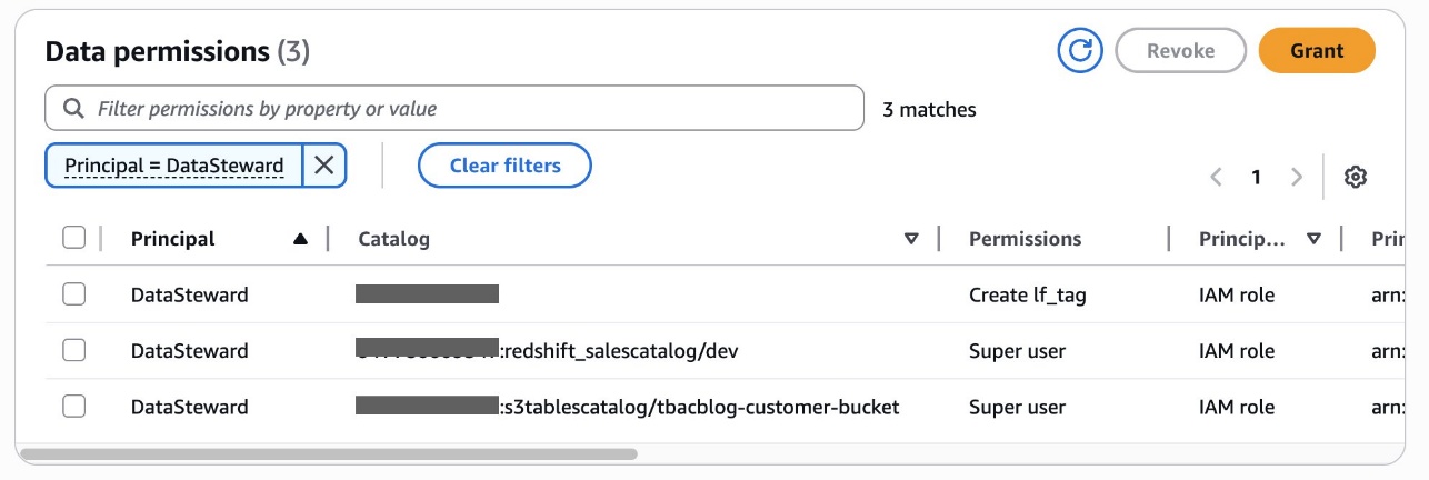
In the pipeline configuration shown in the following screenshot, you can check how OpenSearch Ingestion connects to the HR database. The configuration identifies the source database and the specific tables we want to replicate. While we created a view to understand the data relationships, the pipeline tracks changes from the underlying base tables (employees, departments, locations, and regions). OpenSearch Ingestion automatically maintains these relationships, which means that changes to these tables are properly reflected in your OpenSearch index, keeping your search data consistent with your source database.

In the gif shown below, you can see a demo of setting up this integration using the visual editor of OpenSearch Ingestion.

You can also specify index mapping templates to map your Aurora or Amazon RDS fields to the correct fields in your OpenSearch Service indexes.
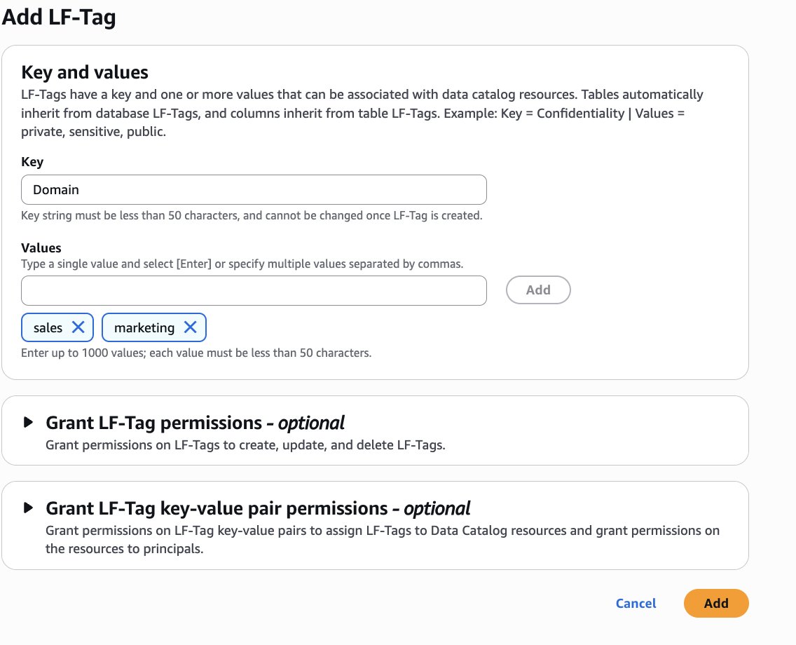
For a comprehensive overview of configuration settings for the pipeline, refer to the OpenSearch Data Prepper documentation. You must set up AWS Identity and Access Management (IAM) roles for the pipeline. For instructions, refer to Configure the pipeline role.

After you configure the integration in OpenSearch Ingestion, the pipeline automatically creates indexes that you can view in OpenSearch Dashboards. OpenSearch Ingestion first triggers an automatic export of your Aurora or Amazon RDS database to Amazon S3, then loads this snapshot data from S3 into your OpenSearch cluster to create the initial indices. After this initial load, OpenSearch Ingestion continually captures changes using binary logs (binlog) for MySQL-based databases or write-ahead logs (WAL) for PostgreSQL-based databases. This way, your OpenSearch indices stay synchronized with your source database in near real time. You can view your indices in OpenSearch Dashboards by invoking:
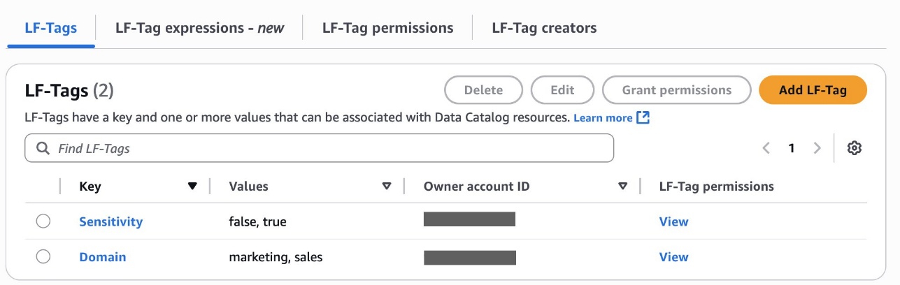
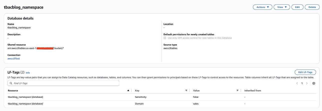
GET _cat/indices

Example response:

Demonstrating near real time data synchronization

Consider the first five entries in the employee table:

When you make changes to your database, OpenSearch Ingestion updates Amazon OpenSearch Service with the change data. For example, the following code updates an employee’s salary:

UPDATE hr.employees SET SALARY = 26000 WHERE EMPLOYEE_ID = 100;

Amazon Aurora sends out a change notice, your OpenSearch Ingestion pipeline picks it up, and OpenSearch Ingestion sends the changed record to OpenSearch in near real time. You can verify this with an OpenSearch query:

GET employees/_search

Important details about this feature:

  • Monitoring – Track pipeline performance and data synchronization through CloudWatch metrics and the OpenSearch Ingestion dashboard
  • Limitations – Requires same-Region and same-account deployment, primary keys for optimal synchronization, and currently has no data definition language (DDL) statement support

Conclusion

Amazon Aurora or Amazon RDS integration with Amazon OpenSearch Service is now generally available in all AWS Regions where OpenSearch Ingestion is available.

To learn more, refer to the AWS documentation for Aurora or Amazon RDS integration with Amazon OpenSearch Service:


About the authors

Michael Torio is an Associate Specialist Solutions Architect at AWS focused on Amazon OpenSearch Service based out of Mountain View, CA. Michael enjoys helping customers leverage cloud technologies to solve their business challenges.

Sohaib Katariwala is a Senior Specialist Solutions Architect at AWS focused on Amazon OpenSearch Service based out of Chicago, IL. His interests are in all things data and analytics. More specifically he loves to help customers use AI in their data strategy to solve modern day challenges.

Arjun Nambiar is a Product Manager with Amazon OpenSearch Service. He focuses on ingestion technologies that enable ingesting data from a wide variety of sources into Amazon OpenSearch Service at scale. Arjun is interested in large-scale distributed systems and cloud-centered technologies, and is based out of Seattle, Washington.

Scale your AWS Glue for Apache Spark jobs with R type, G.12X, and G.16X workers

Post Syndicated from Noritaka Sekiyama original https://aws.amazon.com/blogs/big-data/scale-your-aws-glue-for-apache-spark-jobs-with-r-type-g-12x-and-g-16x-workers/

With AWS Glue, organizations can discover, prepare, and combine data for analytics, machine learning (ML), AI, and application development. At its core, AWS Glue for Apache Spark jobs operate by specifying your code and the number of Data Processing Units (DPUs) needed, with each DPU providing computing resources to power your data integration tasks. However, although the existing workers effectively serve most data integration needs, today’s data landscapes are becoming increasingly complex at larger scale. Organizations are dealing with larger data volumes, more diverse data sources, and increasingly sophisticated transformation requirements.

Although horizontal scaling (adding more workers) effectively addresses many data processing challenges, certain workloads benefit significantly from vertical scaling (increasing the capacity of individual workers). These scenarios include processing large, complex query plans, handling memory-intensive operations, or managing workloads that require substantial per-worker resources for operations such as large join operations, complex aggregations, and data skew scenarios. The ability to scale both horizontally and vertically provides the flexibility needed to optimize performance across diverse data processing requirements.

Responding to these growing demands, today we are pleased to announce the general availability of AWS Glue R type, G.12X, and G.16X workers, the new AWS Glue worker types for the most demanding data integration workloads. G.12X and G.16X workers offer increased compute, memory, and storage, making it possible for you to vertically scale and run even more intensive data integration jobs. R type workers offer increased memory to meet even more memory-intensive requirements. Larger worker types not only benefit the Spark executors, but also in cases where the Spark driver needs larger capacity—for instance, because the job query plan is large. To learn more about Spark driver and executors, see Key topics in Apache Spark.

This post demonstrates how AWS Glue R type, G.12X, and G.16X workers help you scale up your AWS Glue for Apache Spark jobs.

R type workers

AWS Glue R type workers are designed for memory-intensive workloads where you need more memory per worker than G worker types. G worker types run with a 1:4 vCPU to memory (GB) ratio, whereas R worker types run with a 1:8 vCPU to memory (GB) ratio. R.1X workers provide 1 DPU, with 4 vCPU, 32 GB memory, and 94 GB of disk per node. R.2X workers provide 2 DPU, with 8 vCPU, 64 GB memory, and 128 GB of disk per node. R.4X workers provide 4 DPU, with 16 vCPU, 128 GB memory, and 256 GB of disk per node. R.8X workers provide 8 DPU, with 32 vCPU, 256 GB memory, and 512 GB of disk per node. As with G worker types, you can choose R type workers with a single parameter change in the API, AWS Command Line Interface (AWS CLI), or AWS Glue Studio. Regardless of the worker used, the AWS Glue jobs have the same capabilities, including automatic scaling and interactive job authoring using notebooks. R type workers are available with AWS Glue 4.0 and 5.0.

The following table shows compute, memory, disk, and Spark configurations for each R worker type.

AWS Glue Worker Type DPU per Node vCPU Memory (GB) Disk (GB) Approximate Free Disk Space (GB) Number of Spark Executors per Node Number of Cores per Spark Executor
R.1X 1 4 32 94 44 1 4
R.2X 2 8 64 128 78 1 8
R.4X 4 16 128 256 230 1 16
R.8X 8 32 256 512 485 1 32

To use R type workers on an AWS Glue job, change the setting of the worker type parameter. In AWS Glue Studio, you can choose R 1X, R 2X, R 4X, or R 8X under Worker type.

In the AWS API or AWS SDK, you can specify R worker types in the WorkerType parameter. In the AWS CLI, you can use the --worker-type parameter in a create-job command.

To use R worker types on an AWS Glue Studio notebook or interactive sessions, set R.1X, R.2X, R.4X, or R.8X in the %worker_type magic:

R type workers are priced at $0.52 per DPU-hour for each job, billed per second with a 1-minute minimum.

G.12X and G.16X workers

AWS Glue G.12X and G.16X workers give you more compute, memory, and storage to run your most demanding jobs. G.12X workers provide 12 DPU, with 48 vCPU, 192 GB memory, and 768 GB of disk per worker node. G.16X workers provide 16 DPU, with 64 vCPU, 256 GB memory, and 1024 GB of disk per node. G.16x is double the resources of the existing largest worker type G.8X. You can enable G.12X and G.16X workers with a single parameter change in the API, AWS CLI, or AWS Glue Studio. Regardless of the worker used, the AWS Glue jobs have the same capabilities, including automatic scaling and interactive job authoring using notebooks. G.12X and G.16X workers are available with AWS Glue 4.0 and 5.0.The following table shows compute, memory, disk, and Spark configurations for each G worker type.

AWS Glue Worker Type DPU per Node vCPU Memory (GB) Disk (GB) Approximate Free Disk Space (GB) Number of Spark Executors per Node Number of Cores per Spark Executor
G.025X 0.25 2 4 84 34 1 2
G.1X 1 4 16 94 44 1 4
G.2X 2 8 32 138 78 1 8
G.4X 4 16 64 256 230 1 16
G.8X 8 32 128 512 485 1 32
G.12X (new) 12 48 192 768 741 1 48
G.16X (new) 16 64 256 1024 996 1 64

To use G.12X and G.16X workers on an AWS Glue job, change the setting of the worker type parameter to G.12X or G.16X. In AWS Glue Studio, you can choose G 12X or G 16X under Worker type.

In the AWS API or AWS SDK, you can specify G.12X or G.16X in the WorkerType parameter. In the AWS CLI, you can use the --worker-type parameter in a create-job command.

To use G.12X and G.16X on an AWS Glue Studio notebook or interactive sessions, set G.12X or G.16X in the %worker_type magic:

G type workers are priced at $0.44 per DPU-hour for each job, billed per second with a 1-minute minimum. This is the same pricing as the existing worker types.

Choose the right worker type for your workload

To optimize job resource utilization, run your expected application workload to identify the ideal worker type that aligns with your application’s requirements. Start with general worker types like G.1X or G.2X, and monitor your job run from AWS Glue job metrics, observability metrics, and Spark UI. For more details about how to monitor the resource metrics for AWS Glue jobs, see Best practices for performance tuning AWS Glue for Apache Spark jobs.

When your data processing workload is well distributed across workers, G.1X or G.2X work very well. However, some workloads might require more resources per worker. You can use the new G.12X, G.16X, and R type workers to address them. In this section, we discuss typical use cases where vertical scaling is effective.

Large join operations

Some joins might involve large tables where one or both sides need to be broadcast. Multi-way joins require multiple large datasets to be held in memory. With skewed joins, certain partition keys have disproportionately large data volumes. Horizontal scaling doesn’t help when the entire dataset needs to be in memory on each node for broadcast joins.

High-cardinality group by operations

This use case includes aggregations on columns with many unique values, operations requiring maintenance of large hash tables for grouping, and distinct counts on columns with high uniqueness. High-cardinality operations often result in large hash tables that need to be maintained in memory on each node. Adding more nodes doesn’t reduce the size of these per-node data structures.

Window functions and complex aggregations

Some operations might require a large window frame, or involve computing percentiles, medians, or other rank-based analytics across large datasets, in addition to complex grouping sets or CUBE operations on high-cardinality columns. These operations often require keeping large portions of data in memory per partition. Adding more nodes doesn’t reduce the memory requirement for each individual window or grouping operation.

Complex query plans

Complex query plans can have many stages and deep dependency chains, operations requiring large shuffle buffers, or multiple transformations that need to maintain large intermediate results. These query plans often involve large amounts of intermediate data that need to be held in memory. More nodes don’t necessarily simplify the plan or reduce per-node memory requirements.

Machine learning and complex analytics

With ML and analytics use cases, model training might involve large feature sets, wide transformations requiring substantial intermediate data, or complex statistical computations requiring entire datasets in memory. Many ML algorithms and complex analytics require the entire dataset or large portions of it to be processed together, which can’t be effectively distributed across more nodes.

Data skew scenarios

In some data skew scenarios, you might have to process heavily skewed data where certain partitions are significantly larger, or perform operations on datasets with high-cardinality keys, leading to uneven partition sizes. Horizontal scaling can’t address the fundamental issue of data skew, where some partitions remain much larger than others regardless of the number of nodes.

State-heavy stream processing

State-heavy stream processing can include stateful operations with large state requirements, windowed operations over streaming data with large window sizes, or processing micro-batches with complex state management. Stateful stream processing often requires maintaining large amounts of state per key or window, which can’t be easily distributed across more nodes without compromising the integrity of the state.

In-memory caching

These scenarios might include large datasets that must be be cached for repeated access, iterative algorithms requiring multiple passes over the same data, or caching large datasets for fast access, which often requires keeping substantial portions of data in each node’s memory. Horizontal scaling might not help if the entire dataset needs to be cached on each node for optimal performance.

Data skew example scenarios

Several common patterns can typically cause data skew, such as sorting or groupBy transformations on columns with non-uniformed value distributions, and join operations where certain keys appear more frequently than other keys.

In the following example, we compare the behavior with two different worker types, G.2X and R.2X in the same sample workload to process skewed data.

With G.2X workers

With the G.2X worker type, an AWS Glue job with 10 workers failed due to a No space on left device error while writing records into Amazon Simple Storage Service (Amazon S3). This was mainly caused by large shuffling on a specific column. The following Spark UI view shows the job details.

The Jobs tab shows two completed jobs and one active job where 8 tasks failed out of 493 tasks. Let’s drill down to the details.

The Executors tab shows an uneven distribution of data processing across the Spark executors, which indicates data skew in this failed job. Executors with IDs 2, 7, and 10 have failed tasks and read approximately 64.5 GiB of shuffle data as shown in the Shuffle Read column. In contrast, the other executors show 0.0 B of shuffle data in the Shuffle Read column.

The G.2X worker type can handle most Spark workloads such as data transformations and join operations. However, in this example, there was significant data skew, which caused certain executors to fail due to exceeding the allocated memory.

With R.2X workers

With the R.2X worker type, an AWS Glue job with 10 workers successfully ran without any failures. The number of workers is the same as the previous example—the only difference is the worker type. R workers have two times more memory compared to G workers. The following Spark UI view shows more details.

The Jobs tab shows three completed jobs. No failures are shown on this page.

The Executors tab shows no failed tasks per executor even though there’s an uneven distribution of shuffle reads across executors.

The results showed that R.2X workers successfully completed the workload that failed on G.2X workers using the same number of executors but with the additional memory capacity to handle the skewed data distribution.

Conclusion

In this post, we demonstrated how AWS Glue R type, G.12X, and G.16X workers can help you vertically scale your AWS Glue for Apache Spark jobs. You can start using the new R type, G.12X, and G.16X workers to scale your workload today. For more information on these new worker types and AWS Regions where the new workers are available, visit the AWS Glue documentation.

To learn more, see Getting Started with AWS Glue.


About the Authors

Noritaka Sekiyama is a Principal Big Data Architect with AWS Analytics services. He’s responsible for building software artifacts to help customers. In his spare time, he enjoys cycling on his road bike.

Tomohiro Tanaka is a Senior Cloud Support Engineer at Amazon Web Services. He’s passionate about helping customers use Apache Iceberg for their data lakes on AWS. In his free time, he enjoys a coffee break with his colleagues and making coffee at home.

Peter Tsai is a Software Development Engineer at AWS, where he enjoys solving challenges in the design and performance of the AWS Glue runtime. In his leisure time, he enjoys hiking and cycling.

Matt Su is a Senior Product Manager on the AWS Glue team. He enjoys helping customers uncover insights and make better decisions using their data with AWS Analytics services. In his spare time, he enjoys skiing and gardening.

Sean McGeehan is a Software Development Engineer at AWS, where he builds features for the AWS Glue fulfillment system. In his leisure time, he explores his home of Philadelphia and work city of New York.

Orchestrate data processing jobs, querybooks, and notebooks using visual workflow experience in Amazon SageMaker

Post Syndicated from Naohisa Takahashi original https://aws.amazon.com/blogs/big-data/orchestrate-data-processing-jobs-querybooks-and-notebooks-using-visual-workflow-experience-in-amazon-sagemaker/

Automation of data processing and data integration tasks and queries is essential for data engineers and analysts to maintain up-to-date data pipelines and reports. Amazon SageMaker Unified Studio is a single data and AI development environment where you can find and access the data in your organization and act on it using the ideal tools for your use case. SageMaker Unified Studio offers multiple ways to integrate with data through the Visual ETL, Query Editor, and JupyterLab builders. SageMaker is natively integrated with Apache Airflow and Amazon Managed Workflows for Apache Airflow (Amazon MWAA), and is used to automate the workflow orchestration for jobs, querybooks, and notebooks with a Python-based DAG definition.

Today, we are excited to launch a new visual workflows builder in SageMaker Unified Studio. With the new visual workflow experience, you don’t need to code the Python DAGs manually. Instead, you can visually define the orchestration workflow in SageMaker Unified Studio, and the visual definition is automatically converted to a Python DAG definition that is supported in Airflow. This post demonstrates the new visual workflow experience in SageMaker Unified Studio.

Example use case

In this post, a fictional ecommerce company sells many different products, like books, toys, and jewelry. Customers can leave reviews and star ratings for each product so other customers can make informed decisions about what they should buy. We use a sample synthetic review dataset for demonstration purposes, which includes different products and customer reviews.In this example, we demonstrate the new visual workflow experience with a data processing job, SQL querybook, and notebook. We also identify the top 10 customers who have contributed the most helpful votes per category.The following diagram illustrates the solution architecture.

In the following sections, we show how to configure a series of components using data processing jobs, querybooks, and notebooks with SageMaker Unified Studio visual workflows. You can use sample data to extract information from the specific category, update partition metadata, and display query results in the notebook using Python code.

Prerequisites

To get started, you must have the following prerequisites:

  • An AWS account
  • A SageMaker Unified Studio domain. To use the sample data provided in this blog post, your domain should be in us-east-1 region.
  • A SageMaker Unified Studio project with the Data analytics and AI-ML model development project profile
  • A workflow environment

Create a data processing job

The first step is to create a data processing job to run visual transformations to identify top contributing customers per category. Complete the following steps to create a data processing job:

  1. On the top menu, under Build, choose Visual ETL flow.
  2. Choose the plus sign, and under Data sources, choose Amazon S3.
  3. Choose the Amazon S3 source node and enter the following values:
    1. S3 URI: s3://aws-bigdata-blog/generated_synthetic_reviews/data/
    2. Format: Parquet
  4. Choose Update node.
  5. Choose the plus sign, and under Transform, choose Filter.
  6. Choose the Filter node and enter the following values:
    1. Filter Type: Global AND
    2. Key: product_category
    3. Operation: ==
    4. Value: Books
  7. Choose Update node.
  8. Choose the plus sign, and under Data targets, choose Amazon S3.
  9. Choose the S3 node and enter the following values:
    1. S3 URI: Use the Amazon S3 location from the project overview page and add the suffix /data/books_synthetic_reviews/ (for example, /dzd_al0ii4pi2sqv68/awi0lzjswu0yhc/dev/data/books_synthetic_reviews/)
    2. Format: Parquet
    3. Compression: Snappy
    4. Partition keys: marketplace
    5. Mode: Overwrite
    6. Update Catalog: True
    7. Database: Choose your database
    8. Table: books_synthetic_review
    9. Include header: False
  10. Choose Update node.

At this point, you should have an end-to-end visual flow. Now you can publish it.

  1. Choose Save to project to save the draft flow.
  2. Change Job name to filter-books-synthetic-review, then choose Update.

The data processing job has been successfully created.

Create a querybook

Complete the following steps to create a querybook to run a SQL query against the source table to recognize partitions:

  1. Choose the plus sign next to the querybook tab to open new querybook.
  2. Enter the following query and choose Save to project. The query MSCK REPAIR TABLE is prepared for recognizing partitions in the table. We don’t run this querybook yet because the querybook is designed to be triggered by a workflow.

MSCK REPAIR TABLE `books_synthetic_review`;

  1. For Querybook title, enter QueryBook-synthetic-review-<timestamp>, then choose Save changes.

The querybook to recognize new partitions has been successfully created.

Create a notebook

Next, we create notebook to generate output and visualize the results. Complete following steps:

  1. On the top menu, under Build, choose JupyterLab.
  2. Choose File, New, and Notebook to create a new notebook.
  3. Enter the following code snippets into notebook cells and save them (provide your AWS account ID, AWS Region, and S3 bucket):
import sys
!{sys.executable} -m pip install PyAthena
from sagemaker_studio import Project
from pyathena import connect
import pandas as pd

project = Project()
s3_path = f'{project.s3.root}/sys/athena/'
region = project.connection().physical_endpoints[0].aws_region
database = project.connection().catalog().databases[0].name

conn = connect(s3_staging_dir=s3_path, region_name=region)

print("Top 10 most helpful commented customer, Books category")
df = pd.read_sql(f"""
select customer_id, sum(helpful_votes) helpful_votes_sum from {database}.books_synthetic_review group by customer_id order by sum(helpful_votes) desc limit 10;
""", conn)
df
  1. Choose File, Save Notebook.

  1. Rename the file name, and choose Rename and Save.
  2. Choose the Git sidebar and choose the plus sign next to the file name.

  1. Enter the commit message and choose COMMIT.
  2. Choose Push to Remote.

Create a workflow

Complete the following steps to create a workflow:

  1. On the top menu, under Build, choose Workflows.
  2. Choose Create new workflow.

  1. Choose the plus sign, then choose Data processing job.

  1. Choose the Data processing job node, then choose Browse jobs.
  2. Select filter-books-synthetic-review and choose Select.

  1. Choose the plus sign, then choose Querybook.
  2. Choose the Querybook node, then choose Browse files.
  3. Select QueryBook-synthetic-review-<timestamp>.sqlnb and choose Select.
  4. Choose the plus sign, then choose Notebook.
  5. Choose the Notebook node, then choose Browse files.
  6. Select synthetics-review-result.ipynb and choose Select.

At this point, you should have an end-to-end visual workflow. Now you can publish it.

  1. Choose Save to project to save the draft flow.
  2. Change Workflow name to synthetic-review-workflow and choose Save to project.

Run the workflow

To run your workflow, complete following steps:

  1. Choose Run on the workflow details page.

  1. Choose View runs to see the running workflow.

When the run is complete, you can check the notebook task result by choosing the run ID (manual__<timestamp>), then choose the notebook task ID (notebook-task-xxxx).

You can find the IDs of the top 10 customers who have contributed the most helpful votes in the notebook output.

Clean up

To avoid incurring future charges, clean up the resources you created during this walkthrough:

  1. On the workflows page, select your workflow, and under Actions, choose Delete workflow.

  1. On the Visual ETL flows page, select filter-books-synthetics-review, and under Actions, choose Delete flow.
  2. In Query Editor, enter and run the following SQL to drop table:
DROP TABLE `books_synthetic_review`;
  1. In JupyterLab, in the File Browser sidebar, choose (right-click) each notebook (synthetics-review-result.ipynb and QueryBook-synthetic-review-<timestamp>.sqlnb) and choose Delete.
  2. Commit with git and then push to the remote repository.

Conclusion

The new visual workflow editor in SageMaker Unified Studio can help you orchestrate your data integration tasks visually without requiring deep expertise in Airflow. Through the visual interface, data engineers and analysts can focus on their core tasks instead of spending time on manual workflow Python DAG code implementation.Visual workflows offer several advantages, including an intuitive visual interface for workflow design and automatic conversion of visual workflows to Python DAG definitions. The integration with Airflow and Amazon MWAA further enhances the utility, and improved monitoring capabilities provide greater visibility into workflow runs. These features contribute to reduced development time in workflow creation. Visual workflows make workflow automation easy for a variety of use cases, such as data engineers orchestrating complex ETL pipelines or analysts maintaining regular reports.We encourage you to explore visual workflows in SageMaker Unified Studio, and discover how they can streamline your data processing and analytics workflows. For more information about SageMaker Unified Studio and its features, see AWS documentation.


About the authors

Naohisa Takahashi is a Senior Cloud Support Engineer on the AWS Support Engineering team. He supports customers resolve technical issues and launch systems. In his spare time, he plays board games with his friends.

Noritaka Sekiyama is a Principal Big Data Architect with AWS Analytics services. He’s responsible for building software artifacts to help customers. In his spare time, he enjoys cycling on his road bike.

Iris Tian is a UX designer on the Amazon SageMaker Unified Studio team. She designs intuitive, end-to-end experiences that simplify and streamline workflows across data processing and orchestration. In her spare time, she enjoys snowboarding and visiting museums.

Regan Baum is a Senior Software Development Engineer on the Amazon SageMaker Unified Studio team. She designs, implements, and maintains features that enable customers to manage their workflows in SageMaker Unified Studio. Outside of work, she enjoys hiking and running.

Yuhang Huang is a Software Development Manager on the Amazon SageMaker Unified Studio team. He leads the engineering team to design, build, and operate scheduling and orchestration capabilities in SageMaker Unified Studio. In his free time, he enjoys playing tennis.
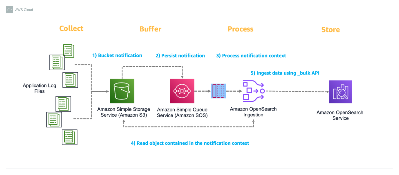
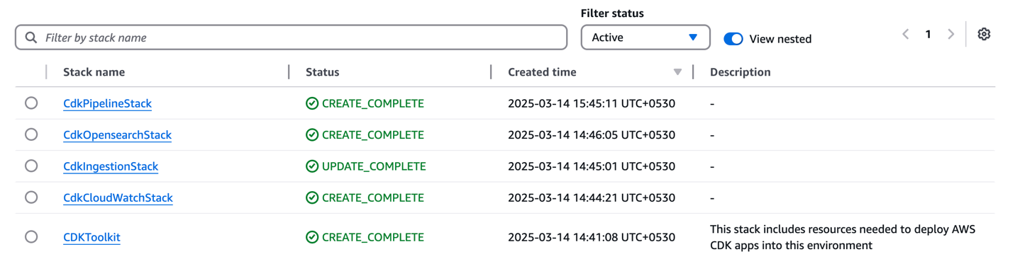
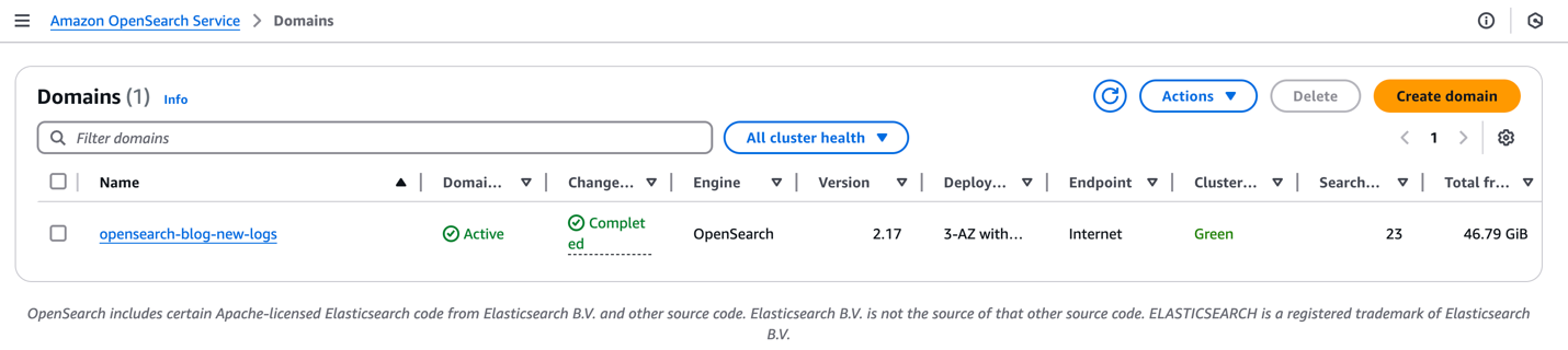
Gal Heyne is a Senior Technical Product Manager for AWS Analytics services with a strong focus on AI/ML and data engineering. She is passionate about developing a deep understanding of customers’ business needs and collaborating with engineers to design simple-to-use data products.

Near real-time baggage operational insights for airlines using Amazon Kinesis Data Streams

Post Syndicated from Subhash Sharma original https://aws.amazon.com/blogs/big-data/near-real-time-baggage-operational-insights-for-airlines-using-amazon-kinesis-data-streams/

To provide a seamless travel experience, aviation enterprises must streamline baggage handling to be as efficient as possible. Traditional baggage analytics systems often struggle with adaptability, real-time insights, data integrity, operational costs, and security, limiting their effectiveness in dynamic environments. Real-time analytics can help in several aspects, such as improving staffing decisions, baggage rerouting, payload planning, and predictive maintenance of Internet of Things (IoT) sensors and belt loaders.

In this post, we explore a framework developed by IBM to modernize baggage analytics using Amazon Web Services (AWS) managed services such as Amazon Kinesis Data Streams, Amazon DynamoDB Streams, Amazon Managed Service for Apache Flink, Amazon QuickSight, Amazon Q in QuickSight, AWS Glue, Amazon SageMaker, and Amazon Aurora within a serverless architecture. This approach delivers significant cost savings, enhanced scalability, and improved performance while providing better security and operational efficiency to meet the evolving needs of airlines. Before diving into the solution’s architecture, we first examine the traditional baggage analytics process and the need for modernization.

Importance of baggage analytics

Baggage management is a process that starts at baggage check-in and ends with the passenger claiming their baggage in a happy path scenario. The following figure explains the high-level baggage management process and respective key performance indicators (KPI). The illustration highlights the critical role of payload planning (part 1), baggage loading (part 2), and below wing payload closeout (part 3) in the flight departure process, all of which directly impact the flight on-time departure metric (part 4). Enhancing the KPIs associated with these essential steps is vital for airlines to optimize operations.

Baggage analytics KPIs

Figure 1: Baggage analytics KPIs

Common KPIs for baggage loading include baggage handling time, turnaround time impact, mishandled baggage rate, baggage accuracy rate, and baggage loading error rate. Similarly, the baggage check-in process plays a crucial role in enhancing the passenger experience. Analyzing variations in this metric across different stations and time periods provides valuable insights for identifying potential bottlenecks and improving efficiency.Airlines can measure performance KPIs using the following business process metrics:

  • Wait times – Wait times are the duration that a process step is waiting on an upstream dependency and are an important factor affecting the overall wait time. Analytics can help identify the potential areas (for example, stations, bag rooms, pier locations, belt loaders, or baggage types) where the processes and system can be fine-tuned to improve the overall wait time.
  • Error rate – Error rate is the time spent on correcting errors or defects. Within these processes, error rate is usually a result of data inconsistencies across multiple systems, manual data entries because of system unavailability or limited aircraft turn-around time, and inconsistencies between payload planning rules and loading procedures. Analytics can help classify these errors among system availability issues, outdated rules, inconsistent data between systems, and other factors. The classification can help prioritize fine-tuning and removing redundancies across systems, rules, and data.
  • Rework time – Rework time is time spent on correcting errors or defects. It can be improved but can’t be avoided, considering last-minute baggage, wheelchairs, ski equipment, and ship or aircraft changes that result in a new payload plan. Analytics can help classify the type, time, and frequency of rework activities across stations, staff members, baggage types, and scenarios related to flight delays and ship changes.
  • Cycle time – Cycle time is the time it takes to complete the process. You can improve the payload planning process cycle time by automating the payload distribution process. To do so, you need to identify and improve the time taken by the payload planning, loading, and closeout processes to reduce the complete departure process cycle time. In many cases, you can improve cycle time by adjusting the processes and adding extra resources, such as workforce, or in other cases by introducing automation. Analytics can identify these time-consuming steps and can be extended to use predictive models to apply mitigation strategies.

Traditional baggage analytics

As explained in the following figure, the traditional baggage handling solution uses monolithic databases with several upstream and downstream dependencies. Upstream dependencies include bags, flight and passenger event feeds to subscribe to the real-time changes in flight, checked bags, and passenger itinerary changes. Downstream dependencies include staffing and customer notifications. The core application interfaces include belt loaders, IoT devices, kiosks, handheld scanners, and web applications for monitoring and reporting. The airline typically stores the reports in the operational database referred to in the diagram as baggage handling (relational database), retaining historical data spanning multiple years, and makes them available to all personnel on the airline’s network. The traditional approach to baggage analytics entails nightly processing of data batches into an enterprise data warehouse (EDW) to generate performance metrics related to airlines’ baggage handling processes.

Traditional baggage analytics

Figure 2: Traditional baggage analytics

Need for modernization

Modernizing baggage analytics is crucial for airlines to achieve growth and enhance operational efficiency. Key factors influencing the modernization are as follows:

  • Inefficiencies in near real-time decision-making – Current systems can’t process and analyze data in real time, leading to delayed responses to operational issues. Integration and data silos hinder insights, preventing proactive decision-making on baggage handling, routing, and anomaly detection.
  • Limitations of traditional ETL solutions – Legacy extract, transform, and load (ETL) processes are batch-driven, slow, and resource-intensive, making them unsuitable for dynamic airline operations. High maintenance costs and frequent failures reduce system reliability and availability.
  • Challenges in proactive anomaly detection and resolution during irregular operations – Airlines struggle to anticipate baggage issues during irregular operations, such as flight delays and weather disruptions. Without predictive analytics, preemptive actions remain a challenge in optimizing staffing, reducing mishandled baggage, and enhancing operational efficiency.

Solution

The modernization of baggage operations must include breaking down the monolithic database into distinct databases based on business capabilities to address performance bottlenecks. Business capabilities can be described as fundamental abilities or competencies that a business possesses and that enable it to achieve its objectives and deliver value to its customers.

As explained in the following figure, the business capabilities for baggage management can be defined as baggage acceptance (check-in), baggage loading, baggage offloading, baggage tracking, baggage mishandling and claims, baggage rerouting, and more. [part 1]. The solution proposes Amazon DynamoDB for an operational database across all baggage management capabilities. DynamoDB global tables provide 99.999% availability with near-zero Recovery Time Objective (RTO) and Recovery Point Objective (RPO), which is crucial for mission-critical baggage handling systems. More details related to baggage operational database modernization can be found at Enhance the reliability of airlines’ mission-critical baggage handling using Amazon DynamoDB in the AWS Database Blog.

The proposed logical solution for baggage operational analytics suggests segregating operational data from historical data, referred to in the diagram as baggage analytics and historical reporting database, to enhance efficiency and alleviate the burden on the operational database [part 3].

Modern baggage analytics

Figure 3: Modern baggage analytics

The solution further uses streaming architecture for the ongoing transfer of data from the operational database to the baggage analytics and historical reporting database [part 2]. This approach aims to facilitate near real-time analytics.The key features for a robust streaming architecture include:

  • Low-latency processing to enable near real-time updates
  • Scalability and elasticity to handle dynamic workloads efficiently
  • Fault tolerance and durability to promote data reliability with replication
  • The ability for multiple consumers to process the same data in parallel at full speed without bottlenecks or interference
  • Exactly one-time processing to avoid duplication and maintain data integrity
  • Ability to replay messages

Real-time streaming on AWS Cloud

The solution uses either Kinesis Data Streams or DynamoDB Streams as a viable streaming solution for processing for change data capture (CDC) within milliseconds. For further information, refer to Streaming options for change data capture and Choose the right change data capture strategy for your Amazon DynamoDB applications.

In this architecture, Kinesis Data Streams is selected to enable fan-out to multiple downstream consumers, extended data retention, and integration with Amazon Managed Service for Apache Flink. Amazon Managed Service for Apache Flink performs stateful stream processing—such as windowed aggregation, filtering, and anomaly detection—before passing data to DynamoDB or Aurora for further analytical aggregation and reporting. Although DynamoDB Streams could also have been used, Kinesis Data Streams provides greater flexibility and throughput for the scale of event processing required here. Additionally, Kinesis Data Streams data retention allows message replays for improved reliability and analysis.

Baggage analytics on AWS Cloud

The solution will use Amazon Simple Storage Service (Amazon S3) for structured and unstructured data storage and Amazon Aurora PostgreSQL-Compatible Edition for relational aggregations. Aurora is well-suited for handling complex aggregations across multiple dimensions (such as month, year, station, and shift) with efficient indexing and SQL functions optimized for reporting. Its relational capabilities support analytical queries needed for performance metrics while providing scalability and efficiency

The following figure explains the high-level cloud architecture for baggage analytics using AWS services.

Baggage real-time analytic architecture on AWS

Figure 4: Near real-time baggage analytics architecture on AWS

The solution can support the following analytics:

  • Interactive and investigative analytics which can produce charts and graphs and discover patterns and anomalies in the baggage data used by product owners. The solution proposes using Amazon QuickSight, which is an interactive tool. Additionally, the solution proposes Amazon Q in QuickSight for natural language queries using a chat-based interface. Amazon QuickSight can be configured using an AWS Glue crawler to automatically discover and extract metadata from various data stores such as Amazon S3 and Amazon Aurora and catalog it in a centralized repository. Amazon QuickSight can be configured to use Amazon Athena to read the data catalog.
  • Predictive analytics used by data scientists involves analyzing historical data to predict future events or behaviors. It uses statistical algorithms and machine learning (ML) techniques to forecast outcomes. The proposed solution is to use a SageMaker notebook to perform predictive analytics on baggage data.

Conclusion

Cloud-based solutions such as Kinesis Data Streams, Athena, and QuickSight revolutionize baggage analytics with scalable, cost-effective infrastructure. By integrating real-time data streaming, analysis, and visualization, they eliminate data silos and enable data-driven decision-making.This modernization optimizes processes, proactively resolving issues to minimize passenger disruptions. Embracing cloud-powered analytics isn’t just a necessity but a strategic step toward greater efficiency, resilience, and customer satisfaction.With this solution, airlines can enhance preemptive issue resolution in baggage operations. Real-time analytics enables better workforce planning, allowing airlines to predict staffing needs at departure and arrival stations, reducing labor costs while ensuring smooth operations. Additionally, data-driven insights help identify inefficiencies during irregular operations, enabling informed decisions for traffic diversion and process optimization.

Check out more AWS Partners or contact an AWS Representative to know how we can help accelerate your business.

Further reading

IBM Consulting is an AWS Premier Tier Services Partner that helps customers who use AWS to harness the power of innovation and drive their business transformation. They are recognized as a Global Systems Integrator (GSI) for over 22 competencies, including travel and hospitality consulting. For more information, please contact an IBM Representative.


About the authors

Neeraj Kaushik is an Open Group Certified Distinguish Architect at IBM with two decades of experience in client-facing delivery roles. His experience spans several industries, including travel and transportation, banking, retail, education, healthcare, and anti-human trafficking. As a trusted advisor, he works directly with the client executive and architects on business strategy to define a technology roadmap. As a hands-on Chief Architect AWS Professional Certified Solution Architect, AWS Certified Machine Learning Specialist and Natural Language Processing Expert, he has led multiple complex cloud modernization programs and AI initiatives.

Jay Pandya is a Senior Partner Solutions Architect in the Global Systems Integrator (GSI) team at Amazon Web Services (AWS). He has over 30 years of IT experience and is helping and providing guidance to AWS GSI partners to build, design, and architect agile, scalable, highly available, and secure solutions on AWS. Outside of the office, Jay enjoys spending time with his family and traveling, and he is an aviation enthusiast and avid sports and Formula 1 fan.

Vijay Gokarn is a Senior Solution Architect at IBM with extensive experience across industries including financial services, healthcare, industrial, retail, and travel and hospitality. He leads complex AWS transformation initiatives, drawing on his hands-on expertise as an AWS Certified Solutions Architect Associate. Vijay specializes in serverless architectures, event-driven systems, and enterprise modernization. As a skilled architect and team leader, he has delivered impactful solutions in cloud modernization, digital banking, and intelligent automation. His passion lies in bridging business strategy with technical execution to drive scalable digital transformation.

Subhash Sharma is Sr. Partner Solutions Architect at AWS. He has more than 25 years of experience in delivering distributed, scalable, highly available, and secured software products using Microservices, AI/ML, the Internet of Things (IoT), and Blockchain using a DevSecOps approach. In his spare time, Subhash likes to spend time with family and friends, hike, walk on beach, and watch TV.

Overcome your Kafka Connect challenges with Amazon Data Firehose

Post Syndicated from Swapna Bandla original https://aws.amazon.com/blogs/big-data/overcome-your-kafka-connect-challenges-with-amazon-data-firehose/

Apache Kafka is a popular open source distributed streaming platform that is widely used in the AWS ecosystem. It’s designed to handle real-time, high-throughput data streams, making it well-suited for building real-time data pipelines to meet the streaming needs of modern cloud-based applications.

For AWS customers looking to run Apache Kafka, but don’t want to worry about the undifferentiated heavy lifting involved with self-managing their Kafka clusters, Amazon Managed Streaming for Apache Kafka (Amazon MSK) offers fully managed Apache Kafka. This means Amazon MSK provisions your servers, configures your Kafka clusters, replaces servers when they fail, orchestrates server patches and upgrades, makes sure clusters are architected for high availability, makes sure data is durably stored and secured, sets up monitoring and alarms, and runs scaling to support load changes. With a managed service, you can spend your time developing and running streaming event applications.

For applications to use data sent to Kafka, you need to write, deploy, and manage application code that consumes data from Kafka.

Kafka Connect is an open-source component of the Kafka project that provides a framework for connecting with external systems such as databases, key-value stores, search indexes, and file systems from your Kafka clusters. On AWS, our customers commonly write and manage connectors using the Kafka Connect framework to move data out of their Kafka clusters into persistent storage, like Amazon Simple Storage Service (Amazon S3), for long-term storage and historical analysis.

At scale, customers need to programmatically manage their Kafka Connect infrastructure for consistent deployments when updates are required, as well as the code for error handling, retries, compression, or data transformation as it is delivered from your Kafka cluster. However, this introduces a need for investment into the software development lifecycle (SDLC) of this management software. Although the SDLC is a cost-effective and time-efficient process to help development teams build high-quality software, for many customers, this process is not desirable for their data delivery use case, particularly when they could dedicate more resources towards innovating for other key business differentiators. Beyond SDLC challenges, many customers face fluctuating data streaming throughput. For instance:

  • Online gaming businesses experience throughput variations based on game usage
  • Video streaming applications see changes in throughput depending on viewership
  • Traditional businesses have throughput fluctuations tied to consumer activity

Striking the right balance between resources and workload can be challenging. Under-provisioning can lead to consumer lag, processing delays, and potential data loss during peak loads, hampering real-time data flows and business operations. On the other hand, over-provisioning results in underutilized resources and unnecessary high costs, making the setup economically inefficient for customers. Even the action of scaling up your infrastructure introduces additional delays because resources need to be provisioned and acquired for your Kafka Connect cluster.

Even when you can estimate aggregated throughput, predicting throughput per individual stream remains difficult. As a result, to achieve smooth operations, you might resort to over-provisioning your Kafka Connect resources (CPU) for your streams. This approach, though functional, might not be the most efficient or cost-effective solution.

Customers have been asking for a fully serverless solution that will not only handle managing resource allocation, but transition the cost model to only pay for the data they are delivering from the Kafka topic, instead of underlying resources that require constant monitoring and management.

In September 2023, we announced a new integration between Amazon and Amazon Data Firehose, allowing builders to deliver data from their MSK topics to their destination sinks with a fully managed, serverless solution. With this new integration, you no longer needed to develop and manage your own code to read, transform, and write your data to your sink using Kafka Connect. Data Firehose abstracts away the retry logic required when reading data from your MSK cluster and delivering it to the desired sink, as well as infrastructure provisioning, because it can scale out and scale in automatically to adjust to the volume of data to transfer. There are no provisioning or maintenance operations required on your side.

At release, the checkpoint time to start consuming data from the MSK topic was the creation time of the Firehose stream. Data Firehose couldn’t start reading from other points on the data stream. This caused challenges for several different use cases.

For customers that are setting up a mechanism to sink data from their cluster for the first time, all data in the topic older than the timestamp of Firehose stream creation would need another way to be persisted. For example, customers using Kafka Connect connectors, like These users were limited in using Data Firehose because they wanted to sink all the data from the topic to their sink, but Data Firehose couldn’t read data from earlier than the timestamp of Firehose stream creation.

For other customers that were running Kafka Connect and needed to migrate from their Kafka Connect infrastructure to Data Firehose, this required some extra coordination. The release functionality of Data Firehose means you can’t point your Firehose stream to a specific point on the source topic, so a migration requires stopping data ingest to the source MSK topic and waiting for Kafka Connect to sink all the data to the destination. Then you can create the Firehose stream and restart the producers such that the Firehose stream can then consume new messages from the topic. This adds additional, and non-trivial, overhead to the migration effort when attempting to cut over from an existing Kafka Connect infrastructure to a new Firehose stream.

To address these challenges, we’re happy to announce a new feature in the Data Firehose integration with Amazon MSK. You can now specify the Firehose stream to either read from the earliest position on the Kafka topic or from a custom timestamp to begin reading from your MSK topic.

In the first post of this series, we focused on managed data delivery from Kafka to your data lake. In this post, we extend the solution to choose a custom timestamp for your MSK topic to be synced to Amazon S3.

Overview of Data Firehose integration with Amazon MSK

Data Firehose integrates with Amazon MSK to offer a fully managed solution that simplifies the processing and delivery of streaming data from Kafka clusters into data lakes stored on Amazon S3. With just a few clicks, you can continuously load data from your desired Kafka clusters to an S3 bucket in the same account, eliminating the need to develop or run your own connector applications. The following are some of the key benefits to this approach:

  • Fully managed service – Data Firehose is a fully managed service that handles the provisioning, scaling, and operational tasks, allowing you to focus on configuring the data delivery pipeline.
  • Simplified configuration – With Data Firehose, you can set up the data delivery pipeline from Amazon MSK to your sink with just a few clicks on the AWS Management Console.
  • Automatic scaling – Data Firehose automatically scales to match the throughput of your Amazon MSK data, without the need for ongoing administration.
  • Data transformation and optimization – Data Firehose offers features like JSON to Parquet/ORC conversion and batch aggregation to optimize the delivered file size, simplifying data analytical processing workflows.
  • Error handling and retries – Data Firehose automatically retries data delivery in case of failures, with configurable retry durations and backup options.
  • Offset select option – With Data Firehose, you can select the starting position for the MSK delivery stream to be delivered within a topic from three options:
    • Firehose stream creation time – This allows you to deliver data starting from Firehose stream creation time. When migrating from to Data Firehose, if you have an option to pause the producer, you can consider this option.
    • Earliest – This allows you to deliver data starting from MSK topic creation time. You can choose this option if you’re setting a new delivery pipeline with Data Firehose from Amazon MSK to Amazon S3.
    • At timestamp – This option allows you to provide a specific start date and time in the topic from where you want the Firehose stream to read data. The time is in your local time zone. You can choose this option if you prefer not to stop your producer applications while migrating from Kafka Connect to Data Firehose. You can refer to the Python script and steps provided later in this post to derive the timestamp for the latest events in your topic that were consumed by Kafka Connect.

The following are benefits of the new timestamp selection feature with Data Firehose:

  • You can select the starting position of the MSK topic, not just from the point that the Firehose stream is created, but from any point from the earliest timestamp of the topic.
  • You can replay the MSK stream delivery if required, for example in the case of testing scenarios to select from different timestamps with the option to select from a specific timestamp.
  • When migrating from Kafka Connect to Data Firehose, gaps or duplicates can be managed by selecting the starting timestamp for Data Firehose delivery from the point where Kafka Connect delivery ended. Because the new custom timestamp feature isn’t monitoring Kafka consumer offsets per partition, the timestamp you select for your Kafka topic should be a few minutes before the timestamp at which you stopped Kafka Connect. The earlier the timestamp you select, the more duplicate records you will have downstream. The closer the timestamp to the time of Kafka Connect stopping, the higher the likelihood of data loss if certain partitions have fallen behind. Be sure to select a timestamp appropriate to your requirements.

Overview of solution

We discuss two scenarios to stream data.

In Scenario 1, we migrate to Data Firehose from Kafka Connect with the following steps:

  1. Derive the latest timestamp from MSK events that Kafka Connect delivered to Amazon S3.
  2. Create a Firehose delivery stream with Amazon MSK as the source and Amazon S3 as the destination with the topic starting position as Earliest.
  3. Query Amazon S3 to validate the data loaded.

In Scenario 2, we create a new data pipeline from Amazon MSK to Amazon S3 with Data Firehose:

  1. Create a Firehose delivery stream with Amazon MSK as the source and Amazon S3 as the destination with the topic starting position as At timestamp.
  2. Query Amazon S3 to validate the data loaded.

The solution architecture is depicted in the following diagram.

Prerequisites

You should have the following prerequisites:

  • An AWS account and access to the following AWS services:
  • An MSK provisioned or MSK serverless cluster with topics created and data streaming to it. The sample topic used in this is order.
  • An EC2 instance configured to use as a Kafka admin client. Refer to Create an IAM role for instructions to create the client machine and IAM role that you will need to run commands against your MSK cluster.
  • An S3 bucket for delivering data from Amazon MSK using Data Firehose.
  • Kafka Connect to deliver data from Amazon MSK to Amazon S3 if you want to migrate from Kafka Connect (Scenario 1).

Migrate to Data Firehose from Kafka Connect

To reduce duplicates and minimize data loss, you need to configure your custom timestamp for Data Firehose to read events as close to the timestamp of the oldest committed offset that Kafka Connect reported. You can follow the steps in this section to visualize how the timestamps of each committed offset will vary by partition across the topic you want to read from. This is for demonstration purposes and doesn’t scale as a solution for workloads with a large number of partitions.

Sample data was generated for demonstration purposes by following the instructions referenced in the following GitHub repo. We set up a sample producer application that generates clickstream events to simulate users browsing and performing actions on an imaginary ecommerce website.

To derive the latest timestamp from MSK events that Kafka Connect delivered to Amazon S3, complete the following steps:

  1. From your Kafka client, query Amazon MSK to retrieve the Kafka Connect consumer group ID:
    ./kafka-consumer-groups.sh --bootstrap-server $bs --list --command-config client.properties

  2. Stop Kafka Connect.
  3. Query Amazon MSK for the latest offset and associated timestamp for the consumer group belonging to Kafka Connect.

You can use the get_latest_offsets.py Python script from the following GitHub repo as a reference to get the timestamp associated with the latest offsets for your Kafka Connect consumer group. To enable authentication and authorization for a non-Java client with an IAM authenticated MSK cluster, refer to the following GitHub repo for instructions on installing the aws-msk-iam-sasl-signer-python package for your client.

python3 get_latest_offsets.py --broker-list $bs --topic-name “order” --consumer-group-id “connect-msk-serverless-connector-090224” --aws-region “eu-west-1”

Note the earliest timestamp across all the partitions.

Create a data pipeline from Amazon MSK to Amazon S3 with Data Firehose

The steps in this section are applicable to both scenarios. Complete the following steps to create your data pipeline:

  1. On the Data Firehose console, choose Firehose streams in the navigation pane.
  2. Choose Create Firehose stream.
  3. For Source, choose Amazon MSK.
  4. For Destination, choose Amazon S3.
  5. For Source settings, browse to the MSK cluster and enter the topic name you created as part of the prerequisites.
  6. Configure the Firehose stream starting position based on your scenario:
    1. For Scenario 1, set Topic starting position as At Timestamp and enter the timestamp you noted in the previous section.
    2. For Scenario 2, set Topic starting position as Earliest.
  7. For Firehose stream name, leave the default generated name or enter a name of your preference.
  8. For Destination settings, browse to the S3 bucket created as part of the prerequisites to stream data.

Within this S3 bucket, by default, a folder structure with YYYY/MM/dd/HH will be automatically created. Data will be delivered to subfolders pertaining to the HH subfolder according to the Data Firehose to Amazon S3 ingestion timestamp.

  1. Under Advanced settings, you can choose to create the default IAM role for all the permissions that Data Firehose needs or choose existing an IAM role that has the policies that Data Firehose needs.
  2. Choose Create Firehose stream.

On the Amazon S3 console, you can verify the data streamed to the S3 folder according to your chosen offset settings.

Clean up

To avoid incurring future charges, delete the resources you created as part of this exercise if you’re not planning to use them further.

Conclusion

Data Firehose provides a straightforward way to deliver data from Amazon MSK to Amazon S3, enabling you to save costs and reduce latency to seconds. To try Data Firehose with Amazon S3, refer to the Delivery to Amazon S3 using Amazon Data Firehose lab.


About the Authors

Swapna Bandla is a Senior Solutions Architect in the AWS Analytics Specialist SA Team. Swapna has a passion towards understanding customers data and analytics needs and empowering them to develop cloud-based well-architected solutions. Outside of work, she enjoys spending time with her family.

Austin Groeneveld is a Streaming Specialist Solutions Architect at Amazon Web Services (AWS), based in the San Francisco Bay Area. In this role, Austin is passionate about helping customers accelerate insights from their data using the AWS platform. He is particularly fascinated by the growing role that data streaming plays in driving innovation in the data analytics space. Outside of his work at AWS, Austin enjoys watching and playing soccer, traveling, and spending quality time with his family.

Build conversational AI search with Amazon OpenSearch Service

Post Syndicated from Bharav Patel original https://aws.amazon.com/blogs/big-data/build-conversational-ai-search-with-amazon-opensearch-service/

Retrieval Augmented Generation (RAG) is a well-known approach to creating generative AI applications. RAG combines large language models (LLMs) with external world knowledge retrieval and is increasingly popular for adding accuracy and personalization to AI. It retrieves relevant information from external sources, augments the input with this data, and generates responses based on both. This approach reduces hallucinations, improves fact accuracy, and allows for up-to-date, efficient, and explainable AI systems. RAG’s ability to break through classical language model limitations has made it applicable to broad AI use cases.

Amazon OpenSearch Service is a versatile search and analytics tool. It is capable of performing security analytics, searching data, analyzing logs, and many other tasks. It can also work with vector data with a k-nearest neighbors (k-NN) plugin, which makes it helpful for more complex search strategies. Because of this feature, OpenSearch Service can serve as a knowledge base for generative AI applications that integrate language generation with search results.

By preserving context over several exchanges, honing responses, and providing a more seamless user experience, conversational search enhances RAG. It helps with complex information needs, resolves ambiguities, and manages multi-turn reasoning. Conversational search provides a more natural and personalized interaction, yielding more accurate and pertinent results, even though standard RAG performs well for single queries.

In this post, we explore conversational search, its architecture, and various ways to implement it.

Solution overview

Let’s walk through the solution to build conversational search. The following diagram illustrates the solution architecture.

The new OpenSearch feature known as agents and tools is used to create conversational search. To develop sophisticated AI applications, agents coordinate a variety of machine learning (ML) tasks. Every agent has a number of tools; each intended for a particular function. To use agents and tools, you need OpenSearch version 2.13 or later.

Prerequisites

To implement this solution, you need an AWS account. If you don’t have one, you can create an account. You also need an OpenSearch Service domain with OpenSearch version 2.13 or later. You can use an existing domain or create a new domain.

To use the Amazon Titan Text Embedding and Anthropic Claude V1 models in Amazon Bedrock, you need to enable access to these foundation models (FMs). For instructions, refer to Add or remove access to Amazon Bedrock foundation models.

Configure IAM permissions

Complete the following steps to set up an AWS Identity and Access Management (IAM) role and user with appropriate permissions:

  1. Create an IAM role with the following policy that will allow the OpenSearch Service domain to invoke the Amazon Bedrock API:
    {
        "Version": "2012-10-17",
        "Statement": [
            {
                "Sid": "Statement1",
                "Effect": "Allow",
                "Action": [
                    "bedrock:InvokeAgent",
                    "bedrock:InvokeModel"
                ],
                "Resource": [
                    "arn:aws:bedrock:${Region}::foundation-model/amazon.titan-embed-text-v1",
                    "arn:aws:bedrock: ${Region}::foundation-model/anthropic.claude-instant-v1"
                ]
            }
        ]
    }
    

Depending on the AWS Region and model you use, specify those in the Resource section.

  1. Add opensearchservice.amazonaws.com as a trusted entity.
  2. Make a note of the IAM role Amazon Resource name (ARN).
  3. Assign the preceding policy to the IAM user that will create a connector.
  4. Create a passRole policy and assign it to IAM user that will create the connector using Python:
    {
        "Version": "2012-10-17",
        "Statement": [
            {
                "Effect": "Allow",
                "Action": "iam:PassRole",
                "Resource": "arn:aws:iam::${AccountId}:role/OpenSearchBedrock"
            }
        ]
    }
  5. Map the IAM role you created to the OpenSearch Service domain role using the following steps:
    • Log in to the OpenSearch Dashboard and open the Security page from the navigation menu.
    • Choose Roles and select ml_all_access.
    • Choose Mapped Users and Manage Mapping.
    • Under Users, add the ARN of the IAM user you created.

Establish a connection to the Amazon Bedrock model using the MLCommons plugin

In order to identify patterns and relationships, an embedding model transforms input data—such as words or images—into numerical vectors in a continuous space. Similar objects are grouped together to make it easier for AI systems to comprehend and respond to intricate user enquiries.

Semantic search concentrates on the purpose and meaning of a query. OpenSearch stores data in a vector index for retrieval and transforms it into dense vectors (lists of numbers) using text embedding models. We are using amazon.titan-embed-text-v1 hosted on Amazon Bedrock, but you will need to evaluate and choose the right model for your use case. The amazon.titan-embed-text-v1 model maps sentences and paragraphs to a 1,536-dimensional dense vector space and is optimized for the task of semantic search.

Complete the following steps to establish a connection to the Amazon Bedrock model using the MLCommons plugin:

  1. Establish a connection by using the Python client with the connection blueprint.
  2. Modify the values of the host and region parameters in the provided code block. For this example, we’re running the program in Visual Studio Code with Python version 3.9.6, but newer versions should also work.
  3. For the role ARN, use the ARN you created earlier, and run the following script using the credentials of the IAM user you created:
    import boto3
    import requests 
    from requests_aws4auth import AWS4Auth
    
    host = 'https://search-test.us-east-1.es.amazonaws.com/'
    region = 'us-east-1'
    service = 'es'
    credentials = boto3.Session().get_credentials()
    awsauth = AWS4Auth(credentials.access_key, credentials.secret_key, region, service, session_token=credentials.token)
    
    path = '_plugins/_ml/connectors/_create'
    url = host + path
    
    payload = {
      "name": "Amazon Bedrock Connector: embedding",
      "description": "The connector to bedrock Titan embedding model",
      "version": 1,
      "protocol": "aws_sigv4",
      "parameters": {
        "region": "us-east-1",
        "service_name": "bedrock",
        "model": "amazon.titan-embed-text-v1"
      },
      "credential": {
        "roleArn": "arn:aws:iam::<accountID>:role/opensearch_bedrock_external"
      },
      "actions": [
        {
          "action_type": "predict",
          "method": "POST",
          "url": "https://bedrock-runtime.${parameters.region}.amazonaws.com/model/${parameters.model}/invoke",
          "headers": {
            "content-type": "application/json",
            "x-amz-content-sha256": "required"
          },
          "request_body": "{ \"inputText\": \"${parameters.inputText}\" }",
          "pre_process_function": "connector.pre_process.bedrock.embedding",
          "post_process_function": "connector.post_process.bedrock.embedding"
        }
      ]
    }
    
    headers = {"Content-Type": "application/json"}
    
    r = requests.post(url, auth=awsauth, json=payload, headers=headers, timeout=15)
    print(r.status_code)
    print(r.text)
    
  4. Run the Python program. This will return connector_id.
    python3 connect_bedrocktitanembedding.py
    200
    {"connector_id":"nbBe65EByVCe3QrFhrQ2"}
  5. Create a model group against which this model will be registered in the OpenSearch Service domain:
    POST /_plugins/_ml/model_groups/_register
    {
      "name": "embedding_model_group",
      "description": "A model group for bedrock embedding models"
    }

    You get the following output:

    {
      "model_group_id": "1rBv65EByVCe3QrFXL6O",
      "status": "CREATED"
    }
  6. Register a model using connector_id and model_group_id:
    POST /_plugins/_ml/models/_register
    {
        "name": "titan_text_embedding_bedrock",
        "function_name": "remote",
        "model_group_id": "1rBv65EByVCe3QrFXL6O",
        "description": "test model",
        "connector_id": "nbBe65EByVCe3QrFhrQ2",
       "interface": {}
    }

You get the following output:

{
  "task_id": "2LB265EByVCe3QrFAb6R",
  "status": "CREATED",
  "model_id": "2bB265EByVCe3QrFAb60"
}
  1. Deploy a model using the model ID:
POST /_plugins/_ml/models/2bB265EByVCe3QrFAb60/_deploy

You get the following output:

{
  "task_id": "bLB665EByVCe3QrF-slA",
  "task_type": "DEPLOY_MODEL",
  "status": "COMPLETED"
}

Now the model is deployed, and you will see that in OpenSearch Dashboards on the OpenSearch Plugins page.

Create an ingestion pipeline for data indexing

Use the following code to create an ingestion pipeline for data indexing. The pipeline will establish a connection to the embedding model, retrieve the embedding, and then store it in the index.

PUT /_ingest/pipeline/cricket_data_pipeline {
    "description": "batting score summary embedding pipeline",
    "processors": [
        {
            "text_embedding": {
                "model_id": "GQOsUJEByVCe3QrFfUNq",
                "field_map": {
                    "cricket_score": "cricket_score_embedding"
                }
            }
        }
    ]
}

Create an index for storing data

Create an index for storing data (for this example, the cricket achievements of batsmen). This index stores raw text and embeddings of the summary text with 1,536 dimensions and uses the ingest pipeline we created in the previous step.

PUT cricket_data {
    "mappings": {
        "properties": {
            "cricket_score": {
                "type": "text"
            },
            "cricket_score_embedding": {
                "type": "knn_vector",
                "dimension": 1536,
                "space_type": "l2",
                "method": {
                    "name": "hnsw",
                    "engine": "faiss"
                }
            }
        }
    },
    "settings": {
        "index": {
            "knn": "true"
        }
    }
}

Ingest sample data

Use the following code to ingest the sample data for four batsmen:

POST _bulk?pipeline=cricket_data_pipeline
{"index": {"_index": "cricket_data"}}
{"cricket_score": "Sachin Tendulkar, often hailed as the 'God of Cricket,' amassed an extraordinary batting record throughout his 24-year international career. In Test cricket, he played 200 matches, scoring a staggering 15,921 runs at an average of 53.78, including 51 centuries and 68 half-centuries, with a highest score of 248 not out. His One Day International (ODI) career was equally impressive, spanning 463 matches where he scored 18,426 runs at an average of 44.83, notching up 49 centuries and 96 half-centuries, with a top score of 200 not out – the first double century in ODI history. Although he played just one T20 International, scoring 10 runs, his overall batting statistics across formats solidified his status as one of cricket's all-time greats, setting numerous records that stand to this day."}
{"index": {"_index": "cricket_data"}}
{"cricket_score": "Virat Kohli, widely regarded as one of the finest batsmen of his generation, has amassed impressive statistics across all formats of international cricket. As of April 2024, in Test cricket, he has scored over 8,000 runs with an average exceeding 50, including numerous centuries. His One Day International (ODI) record is particularly stellar, with more than 12,000 runs at an average well above 50, featuring over 40 centuries. In T20 Internationals, Kohli has maintained a high average and scored over 3,000 runs. Known for his exceptional ability to chase down targets in limited-overs cricket, Kohli has consistently ranked among the top batsmen in ICC rankings and has broken several batting records throughout his career, cementing his status as a modern cricket legend."}
{"index": {"_index": "cricket_data"}}
{"cricket_score": "Adam Gilchrist, the legendary Australian wicketkeeper-batsman, had an exceptional batting record across formats during his international career from 1996 to 2008. In Test cricket, Gilchrist scored 5,570 runs in 96 matches at an impressive average of 47.60, including 17 centuries and 26 half-centuries, with a highest score of 204 not out. His One Day International (ODI) record was equally remarkable, amassing 9,619 runs in 287 matches at an average of 35.89, with 16 centuries and 55 half-centuries, and a top score of 172. Gilchrist's aggressive batting style and ability to change the course of a game quickly made him one of the most feared batsmen of his era. Although his T20 International career was brief, his overall batting statistics, combined with his wicketkeeping skills, established him as one of cricket's greatest wicketkeeper-batsmen."}
{"index": {"_index": "cricket_data"}}
{"cricket_score": "Brian Lara, the legendary West Indian batsman, had an extraordinary batting record in international cricket during his career from 1990 to 2007. In Test cricket, Lara amassed 11,953 runs in 131 matches at an impressive average of 52.88, including 34 centuries and 48 half-centuries. He holds the record for the highest individual score in a Test innings with 400 not out, as well as the highest first-class score of 501 not out. In One Day Internationals (ODIs), Lara scored 10,405 runs in 299 matches at an average of 40.48, with 19 centuries and 63 half-centuries. His highest ODI score was 169. Known for his elegant batting style and ability to play long innings, Lara's exceptional performances, particularly in Test cricket, cemented his status as one of the greatest batsmen in the history of the game."}

Deploy the LLM for response generation

Use the following code to deploy the LLM for response generation. Modify the values of host, region, and roleArn in the provided code block.

  1. Create a connector by running the following Python program. Run the script using the credentials of the IAM user created earlier.
    import boto3
    import requests 
    from requests_aws4auth import AWS4Auth
    
    host = 'https://search-test.us-east-1.es.amazonaws.com/'
    region = 'us-east-1'
    service = 'es'
    credentials = boto3.Session().get_credentials()
    awsauth = AWS4Auth(credentials.access_key, credentials.secret_key, region, service, session_token=credentials.token)
    
    path = '_plugins/_ml/connectors/_create'
    url = host + path
    
    payload = {
      "name": "BedRock Claude instant-v1 Connector ",
      "description": "The connector to BedRock service for claude model",
      "version": 1,
      "protocol": "aws_sigv4",
      "parameters": {
        "region": "us-east-1",
        "service_name": "bedrock",
        "anthropic_version": "bedrock-2023-05-31",
        "max_tokens_to_sample": 8000,
        "temperature": 0.0001,
        "response_filter": "$.completion"
      },
       "credential": {
            "roleArn": "arn:aws:iam::accountId:role/opensearch_bedrock_external"
        },
      "actions": [
        {
          "action_type": "predict",
          "method": "POST",
          "url": "https://bedrock-runtime.${parameters.region}.amazonaws.com/model/anthropic.claude-instant-v1/invoke",
          "headers": {
            "content-type": "application/json",
            "x-amz-content-sha256": "required"
          },
          "request_body": "{\"prompt\":\"${parameters.prompt}\", \"max_tokens_to_sample\":${parameters.max_tokens_to_sample}, \"temperature\":${parameters.temperature},  \"anthropic_version\":\"${parameters.anthropic_version}\" }"
        }
      ]
     }
        
    
    headers = {"Content-Type": "application/json"}
    
    r = requests.post(url, auth=awsauth, json=payload, headers=headers, timeout=15)
    print(r.status_code)
    print(r.text)

If it ran successfully, it would return connector_id and a 200-response code:

200
{"connector_id":"LhLSZ5MBLD0avmh1El6Q"}
  1. Create a model group for this model:
    POST /_plugins/_ml/model_groups/_register
    {
        "name": "claude_model_group",
        "description": "This is an example description"
    }

This will return model_group_id; make a note of it:

{
  "model_group_id": "LxLTZ5MBLD0avmh1wV4L",
  "status": "CREATED"
}
  1. Register a model using connection_id and model_group_id:
    POST /_plugins/_ml/models/_register
    {
        "name": "anthropic.claude-v1",
        "function_name": "remote",
        "model_group_id": "LxLTZ5MBLD0avmh1wV4L",
        "description": "LLM model",
        "connector_id": "LhLSZ5MBLD0avmh1El6Q",
        "interface": {}
    }
    

It will return model_id and task_id:

{
  "task_id": "YvbVZ5MBtVAPFbeA7ou7",
  "status": "CREATED",
  "model_id": "Y_bVZ5MBtVAPFbeA7ovb"
}
  1. Finally, deploy the model using an API:
POST /_plugins/_ml/models/Y_bVZ5MBtVAPFbeA7ovb/_deploy

The status will show as COMPLETED. That means the model is successfully deployed.

{
  "task_id": "efbvZ5MBtVAPFbeA7otB",
  "task_type": "DEPLOY_MODEL",
  "status": "COMPLETED"
}

Create an agent in OpenSearch Service

An agent orchestrates and runs ML models and tools. A tool performs a set of specific tasks. For this post, we use the following tools:

  • VectorDBTool – The agent use this tool to retrieve OpenSearch documents relevant to the user question
  • MLModelTool – This tool generates user responses based on prompts and OpenSearch documents

Use the embedding model_id in VectorDBTool and LLM model_id in MLModelTool:

POST /_plugins/_ml/agents/_register {
    "name": "cricket score data analysis agent",
    "type": "conversational_flow",
    "description": "This is a demo agent for cricket data analysis",
    "app_type": "rag",
    "memory": {
        "type": "conversation_index"
    },
    "tools": [
        {
            "type": "VectorDBTool",
            "name": "cricket_knowledge_base",
            "parameters": {
                "model_id": "2bB265EByVCe3QrFAb60",
                "index": "cricket_data",
                "embedding_field": "cricket_score_embedding",
                "source_field": [
                    "cricket_score"
                ],
                "input": "${parameters.question}"
            }
        },
        {
            "type": "MLModelTool",
            "name": "bedrock_claude_model",
            "description": "A general tool to answer any question",
            "parameters": {
                "model_id": "gbcfIpEByVCe3QrFClUp",
                "prompt": "\n\nHuman:You are a professional data analysist. You will always answer question based on the given context first. If the answer is not directly shown in the context, you will analyze the data and find the answer. If you don't know the answer, just say don't know. \n\nContext:\n${parameters.cricket_knowledge_base.output:-}\n\n${parameters.chat_history:-}\n\nHuman:${parameters.question}\n\nAssistant:"
            }
        }
    ]
}

This returns an agent ID; take note of the agent ID, which will be used in subsequent APIs.

Query the index

We have batting scores of four batsmen in the index. For the first query, let’s specify the player name:

POST /_plugins/_ml/agents/<agent ID>/_execute {
    "parameters": {
        "question": "What is batting score of Sachin Tendulkar ?"
    }
}

Based on context and available information, it returns the batting score of Sachin Tendulkar. Note the memory_id from the response; you will need it for subsequent questions in the next steps.

We can ask a follow-up question. This time, we don’t specify the player name and expect it to answer based on the earlier question:

POST /_plugins/_ml/agents/<agent ID>/_execute {
    "parameters": {
        "question": " How many T20 international match did he play?",
        "next_action": "then compare with Virat Kohlis score",
        "memory_id": "so-vAJMByVCe3QrFYO7j",
        "message_history_limit": 5,
        "prompt": "\n\nHuman:You are a professional data analysist. You will always answer question based on the given context first. If the answer is not directly shown in the context, you will analyze the data and find the answer. If you don't know the answer, just say don't know. \n\nContext:\n${parameters.population_knowledge_base.output:-}\n\n${parameters.chat_history:-}\n\nHuman:always learn useful information from chat history\nHuman:${parameters.question}, ${parameters.next_action}\n\nAssistant:"
    }
}

In the preceding API, we use the following parameters:

  • Question and Next_action – We also pass the next action to compare Sachin’s score with Virat’s score.
  • Memory_id – This is memory assigned to this conversation. Use the same memory_id for subsequent questions.
  • Prompt – This is the prompt you give to the LLM. It includes the user’s question and the next action. The LLM should answer only using the data indexed in OpenSearch and must not invent any information. This way, you prevent hallucination.

Refer to ML Model tool for more details about setting up these parameters and the GitHub repo for blueprints for remote inferences.

The tool stores the conversation history of the questions and answers in the OpenSearch index, which is used to refine answers by asking follow-up questions.

In real-world scenarios, you can map memory_id against the user’s profile to preserve the context and isolate the user’s conversation history.

We have demonstrated how to create a conversational search application using the built-in features of OpenSearch Service.

Clean up

To avoid incurring future charges, delete the resources created while building this solution:

  1. Delete the OpenSearch Service domain.
  2. Delete the connector.
  3. Delete the index.

Conclusion

In this post, we demonstrated how to use OpenSearch agents and tools to create a RAG pipeline with conversational search. By integrating with ML models, vectorizing questions, and interacting with LLMs to improve prompts, this configuration oversees the entire process. This method allows you to quickly develop AI assistants that are ready for production without having to start from scratch.

If you’re building a RAG pipeline with conversational history to let users ask follow-up questions for more refined answers, give it a try and share your feedback or questions in the comments!


About the author

Bharav Patel is a Specialist Solution Architect, Analytics at Amazon Web Services. He primarily works on Amazon OpenSearch Service and helps customers with key concepts and design principles of running OpenSearch workloads on the cloud. Bharav likes to explore new places and try out different cuisines.

Remote access to AWS: A guide for hybrid workforces

Post Syndicated from Itay Meller original https://aws.amazon.com/blogs/security/remote-access-to-aws-a-guide-for-hybrid-workforces/

Amazon Web Services (AWS) customers can enable secure remote access to their cloud resources, supporting business operations with both speed and agility. As organizations embrace flexible work environments, employees can safely connect to AWS resources from various locations using different devices. AWS provides comprehensive security solutions that help organizations maintain strong protection of corporate resources, manage appropriate access controls, and meet compliance requirements while enabling productive remote work environments.

Because there are different types of workloads—from Amazon Elastic Compute Cloud (Amazon EC2) instances to web applications—running in the AWS Cloud, there are correspondingly multiple remote access use cases for using or operating these workloads. For example, access to an EC2 instance and its operating system to perform operations such as troubleshooting, log analysis, and data retrieval. Other use cases require access to web applications such as Jenkins, Salesforce, or the Kubernetes UI deployed on AWS.

To support these use cases, AWS provides multiple services and features that help you address access patterns using different approaches. One of the key challenges that you might face when implementing remote access solutions is understanding the tradeoffs of the different approaches and solutions. This post is designed to help you decide which remote access approach is best for your use-case.

Use cases

In this post, we address the following use cases:

Challenges associated with remote access

  • Cost: The cost of a remote access solution is a key factor for businesses.
  • Increased exposure surface: Securing a VPC with several EC2 instances, S3 buckets, and a database is a different task than securing the identities, devices, and communications channels used for remote access to the infrastructure.
  • Increased risk: Susceptibility to social engineering threats. Humans accessing workloads are the weakest link in any security program, introducing risks to data and infrastructure that otherwise wouldn’t have existed.
  • User experience (UX): The UX is a key factor in remote access. Lacking a well-designed UX can introduce risks by making it difficult to conduct day-to-day operations or respond quickly to incidents that affect users at scale.

A solution to mitigate the risks associated with remote access is to not provide it at certain levels, and you might sometimes choose this approach. In these cases, access to workloads that must be secure is only possible from trusted locations (such as company offices) and managed devices (such as company-issued laptops). For the remainder of this post, we talk about approaches and solutions available for you when you need to provide remote access from various locations and devices.

The different approaches

Before diving deeper into the services and features, let’s explore the different approaches for providing remote access to your users (shown in Figure 1). The main differentiator among them is where the trust boundary lies.

Figure 1: The different approaches along with the corresponding solutions

Figure 1: The different approaches along with the corresponding solutions

  • Network-based approach: Users are given access to your network through VPCs and are granted broad access to the actual target resource, web application, or EC2 instances. The trust boundary in this case is the VPC.
  • Host-based approach: Users have access to the host running the application. This is commonly used for operator access. The trust boundary is the host.
  • Application-based approach: Users access the application using their corporate credentials. This is commonly the case for software as a service (SaaS) applications. The trust boundary is the application.
  • End-user computing approach: End-user computing (EUC) is a combination of technologies, policies, and processes that gives users secure, remote access to applications, desktops, and data that they need to get their work done. Desktops are operated centrally in the cloud and interacted with using streamed pixels to users’ devices. This approach shifts the trust boundary from the user device to desktops and data residing in the cloud.

These approaches aren’t mutually exclusive and occasionally overlap or can be combined in a zero trust model. Zero trust is centered on the idea that access to resources shouldn’t be based solely on the network location but on authentication and authorization of each request using multiple factors; including the user identity, device, and location, among others.

The trust boundary primarily depends on the criticality of the target resource, the risk tolerance of the organization, and the complexity of the implementation. Wider trust boundaries (such as in a network-based approach) increase the exposed surface area—because the whole network is exposed to trusted users and access to the network grants access to all the resources inside it—but are the simplest to implement. Tighter trust boundaries (such as a zero trust model) considerably reduce the exposed surface area but require implementing multiple factors that feed into the authorization context.

For example, organizations might provide network-based access from trusted devices to operators for a VPC with web-servers and databases, but only allow end-user computing based access for contractors or third-party users using non-corporate devices, also known as bring your own device (BYOD).

When selecting your remote access solution, you need to consider the desired trust boundary, authentication, authorization, user experience, access visibility and cost, which we explore in the following sections.

Network-based approach

The network-based approach is popular when users need access to multiple resources residing in specific networks in a straightforward manner, while keeping the networks disconnected from the public internet. When providing access at the network level, managing security configurations such as authorization, authentication, and auditing happens at the resource (application or machine) and client device, introducing challenges at scale.

AWS Client VPN is a fully managed service that you can use to securely connect users to VPCs from virtually any location using OpenVPN-based clients. Users can authenticate using your organization’s identity provider (IdP) in combination with certificate-based authentication. The service supports authorization rules that act as firewall rules to grant users access to specific CIDR blocks based on membership in an Active Directory group or a group defined in a SAML-based IdP. Additionally, you can use client connect handlers to run custom authorization logic based on device, user, and connection attributes.

After the required infrastructure is set up, users can connect to the target VPC and access EC2 instances or web applications at the network level inside their authorization scope. The UX is as straightforward as connecting using client software installed on the user’s device and authenticating using corporate authentication policies. A client VPN provides visibility into users’ connections to the VPN through connection logs, which are streamed to an Amazon CloudWatch log group. Connection logging provides visibility into each user’s initial VPN connection; getting visibility into what happened during the connection requires gathering the data from the target resource, network, or the user’s device.

After the user is authenticated and authorized, their device gains network access to the relevant VPC—and potentially other VPCs that are peered—or is connected through AWS Transit Gateway to that VPC. This can potentially provide network access to resources and networks outside the scope of the user.

A client VPN-based solution should be implemented when the network is the intended trust boundary around resources (for example, at the subnet or security group level) and group-level access control is sufficient. See Get started with AWS Client VPN.

Host-based approach

Providing access to hosts isn’t always necessary. One way to mitigate risks related to unauthorized host access is to not allow it and rely on fully automated operations instead. In practice, operators and developers still require access to hosts for visibility, tuning the operating system settings, applying patches, or manually restarting a service.

For access to EC2 instances, you can use features such as AWS Systems Manager Session Manager or EC2 Instance Connect Endpoint. Both of these features provide access to a host without exposing it to the internet, and because they use AWS Identity and Access Management (IAM), they authenticate, authorize, and log every session request made to AWS CloudTrail, and provide capabilities such as IAM Conditions (for example, aws:SourceIp) to apply conditional access, often minimizing the need for a network-based approach.

These two features mainly differ in the way they operate. Session Manager requires an agent, which is installed by default on several Amazon Machine Images (AMIs). The agent establishes an outbound connection—through the internet or a VPC endpoint—to the service endpoints, so you don’t have to modify the host’s inbound security group rules. It allows SSH connections tunneled over a proxy connection and provides in-session logging providing visibility into users’ commands within a session.

EC2 Instance Connect doesn’t require that you install an agent; it allows a secure native SSH connection, using short-lived SSH keys. As such, it requires that inbound connections from the EC2 Instance Connect service on port 22 be allowed on the host’s security group.

Most customers use Session Manager unless they don’t want to have an agent installed on the virtual machine or require a native SSH experience.

End-user computing approach

End-user computing services like the Amazon WorkSpaces Family or Amazon AppStream 2.0 stream desktops and applications as encrypted pixels to remote users while keeping data safely within your Amazon Virtual Private Cloud (Amazon VPC) and connected private networks. Unauthorized access to the client device is exposed only to encrypted pixels, which essentially moves the trust boundary from the device accessing the resources to the virtual desktop running in the cloud.

You can dive deeper into the differences between these different services in Unified access to AWS End User Computing services.

These services are particularly popular among customers who want to minimize the user’s device as the trust boundary. This can improve operational efficiency, especially when dealing with untrusted devices or highly sensitive data, because you significantly narrow the scope of what needs to be protected. This can also reduce the use (and costs) of expensive hardware.

The idea is that a user first authenticates using credentials provided by the corporate Active Directory or a SAML federation to the corporate identity provider. After the user is authenticated and authorized, an encrypted streaming session begins and the client is remotely operating a desktop or application that’s deployed in an Amazon VPC, with an elastic network interface (ENI) deployed to the customer’s managed VPC.

When adopting end-user computing for remote access, you can choose the UX and the cost structure that best fit your use case (for example, persistent access to a desktop or on-demand access to specific applications). You can also select different compute and storage options depending on the desired performance.

AWS End User Computing provides different machine types to accommodate different UX requirements and with different pricing models depending on the consumption model being used.

For more information, see Getting Started with Amazon Workspaces and Getting Started with AppStream 2.0.

Application-based approach

IAM Identity Center is primarily known for simplifying user access to AWS accounts within an organization at scale. It also provides single sign-on (SSO) access to supported web applications, giving users seamless access to these applications after they sign in using their directory credentials. Identity Center supports two application types:

If you use customer managed applications that support SAML 2.0 and OAuth 2.0, you can federate your IdP to IAM Identity Center through SAML 2.0 and use Identity Center to manage user access to those applications.

For organizations operating AWS environments at scale with multiple accounts, using IAM Identity Center is the recommended service to provide access to web applications and is provided at no additional cost.

Combining multiple approaches in a zero trust model

The zero trust model combines multiple factors including the user identity, device, location, and others, to evaluate and grant access requests. One way that you can implement this model to provide remote access to workloads deployed in a VPC is to use AWS Verified Access. With Verified Access, you can provide secure access to corporate applications without a client VPN and support TCP-based connections to a VPC, be it to web applications or EC2 or RDS instances. Authentication can be done using an existing IdP or AWS IAM Identity Center and a device management service that can provide additional information to improve authorization decisions based on context from the device. Those authorization decisions are expressed as Cedar policies that you author based on your access requirements. The service provides extensive logging for each web request, so you can investigate anomalies and view information about the access that was granted. For more information, see Get Started with Amazon Verified Access.

Understanding the tradeoffs

To select the right solution for your workforce, work backwards from the use case. Start by identifying and classifying the asset inventory and mapping the users accessing it and their access patterns.

Things to consider based on the classification:

  • Visibility: Determine the level of visibility into remote access activities and the type of information that you’ll need to detect and recover from a security event or to comply with regulatory and compliance requirements.
  • Authentication and authorization: Determine if your existing IAM mechanisms are sufficient. You might need to identify a temporary access management system or include information coming from user devices to address risks of compromised employees.
  • Network access: Know your users and what type of network access, if any, they need. When considering network access, include the potential risks of overly permissive access.
  • Cost: To determine costs, you need to know how many users and resources will be supported by remote access. Also, how many connections you expect and for how much time. Use that information to help determine the total cost of ownership of your solution.
  • Endpoint security: For each resource, understand risks associated with providing access to it from a user’s device. Know what mechanisms you have (or can implement) to detect threats and unauthorized access or provide additional context for the authorization decision granting access to a resource.
  • User experience: Compare the cost of a streamed user experience to one that’s locally installed to see if any additional cost is balanced by the improved security of the streamed UX.

The following provides an overview of the different solutions and the factors that can help you make an informed decision.

Solution Use cases Trust Boundary Provides access to Protocol User experience Authentication Authorization Visibility Cost
Client VPN
  • User access to internal applications
  • Operator access to IP resources in VPC
Network VPCs, subnets, security groups IP Client based,native
  • Single sign-on (SAML-based)
  • Active Directory
  • Mutual (certificate based)
  • Per CIDR (Authorization rules)
  • Lambda Authorizer for custom code
Connection logging (CloudWatch) Connection time and endpoint association
AWS Session Manager
  • Operator access to EC2 or on-premises instances
Host EC2 Instances: Linux, Windows, or MacOS (EC2 only) SSH or RDP Native
  • IAM
  • IAM
CloudTrail, or in-session logging using CloudWatch and Amazon S3) No additional cost for accessing EC2 instances
EC2 Instance Connect Endpoint
  • Operator access to EC2 instances
Host EC2 Instances: Linux or Windows SSH or RDP Native
  • IAM
  • IAM
CloudTrail No additional cost
IAM Identity Center
  • User access to SAML 2.0 and OAuth 2.0 applications
Application Web applications HTTP(S) Native
  • IAM Identity Center
  • IAM Identity Center
CloudTrail No additional cost
Amazon Verified Access
  • User accesses web or TCP-based applications deployed in a VPC
Amazon Verified Access
  • Web applications
  • TCP resources
HTTP(S) or TCP Native
  • IAM Identity Center or OIDC
  • Custom using Cedar policies
  • Allows device signals
Per request logging Per application or bandwidth
Amazon Workspaces
  • User accesses a virtual persistent desktop in a VPC
Cloud desktop Persistent virtual desktop WSP or PCoIP Client based, or non-native
  • Identity provider
  • Group membership
CloudTrail Per instance
Amazon AppStream 2.0
  • User accesses a virtual desktop in a VPC
Cloud desktop Non persistent virtual desktops and applications NICE DCV Client based or non-native
  • Identity provider
  • Group membership
CloudTrail Per instance

Conclusion

In this post, you learned about different approaches and solutions for providing remote access for your organization’s workforce. This included tactical recommendations on how to find the remote access solution that suits your needs best based on factors such as costs, user experience, and risk. By understanding those tradeoffs, you can now map out the different use-cases based on your infrastructure and threat model and build a remote access strategy to meet your needs. As you experiment and adopt the different tools, careful planning is required when designing and deploying the services. For example, which account to deploy the service to or how to provision access to the services. Use resources such as the AWS Security Reference Architecture (AWS SRA) and the individual service documentation pages to help guide your journey.

If you have feedback about this post, submit comments in the Comments section below.

Itay Meller

Itay Meller

Itay is a Security Specialist Solutions Architect at AWS, with a strong background in cybersecurity R&D and leadership roles across various security-focused companies. With deep expertise in cloud security, Itay helps organizations securely adopt and scale their AWS environments by addressing complex security and compliance challenges.

Maxim Raya

Maxim Raya

Maxim is a Security Specialist Solutions Architect at AWS. In this role, he helps clients accelerate their cloud transformation by increasing their confidence in the security and compliance of their AWS environments.

Enhance data ingestion performance in Amazon Redshift with concurrent inserts

Post Syndicated from Raghu Kuppala original https://aws.amazon.com/blogs/big-data/enhance-data-ingestion-performance-in-amazon-redshift-with-concurrent-inserts/

Amazon Redshift is a fully managed petabyte data warehousing service in the cloud. Its massively parallel processing (MPP) architecture processes data by distributing queries across compute nodes. Each node executes identical query code on its data portion, enabling parallel processing.

Amazon Redshift employs columnar storage for database tables, reducing overall disk I/O requirements. This storage method significantly improves analytic query performance by minimizing data read during queries. Data has become many organizations’ most valuable asset, driving demand for real-time or near real-time analytics in data warehouses. This demand necessitates systems that support simultaneous data loading while maintaining query performance. This post showcases the key improvements in Amazon Redshift concurrent data ingestion operations.

Challenges and pain points for write workloads

In a data warehouse environment, managing concurrent access to data is crucial yet challenging. Customers using Amazon Redshift ingest data using various approaches. For example, you might commonly use INSERT and COPY statements to load data to a table, which are also called pure write operations. You might have requirements for low-latency ingestions to maximize data freshness. To achieve this, you can submit queries concurrently to the same table. To enable this, Amazon Redshift implements snapshot isolation by default. Snapshot isolation provides data consistency when multiple transactions are running simultaneously. Snapshot isolation guarantees that each transaction sees a consistent snapshot of the database as it existed at the start of the transaction, preventing read and write conflicts that could compromise data integrity. With snapshot isolation, read queries are able to execute in parallel, so you can take advantage of the full performance that the data warehouse has to offer.

However, pure write operations execute sequentially. Specifically, pure write operations need to acquire an exclusive lock during the entire transaction. They only release the lock when the transaction has committed the data. In these cases, the performance of the pure write operations is constrained by the speed of serial execution of the writes across sessions.

To understand this better, let’s look at how a pure write operation works. Every pure write operation includes pre-ingestion tasks such as scanning, sorting, and aggregation on the same table. After the pre-ingestion tasks are complete, the data is written to the table while maintaining data consistency. Because the pure write operations run serially, even the pre-ingestion steps ran serially due to lack of concurrency. This means that when multiple pure write operations are submitted concurrently, they are processed one after another, with no parallelization even for the pre-ingestion steps. To improve the concurrency of ingestion to the same table and meet low latency requirements for ingestion, customers often use workarounds through the use of staging tables. Specifically, you can submit INSERT ... VALUES(..) statements into staging tables. Then, you perform joins with other tables, such FACT and DIMENSION tables, prior to appending data using ALTER TABLE APPEND into your target tables. This approach isn’t desirable because it requires you to maintain staging tables and potentially have a larger storage footprint due to data block fragmentation from the use of ALTER TABLE APPEND statements.

In summary, the sequential execution of concurrent INSERT and COPY statements, due to their exclusive locking behavior, creates challenges if you want to maximize the performance and efficiency of your data ingestion workflows in Amazon Redshift. To overcome these limitations, you must adopt workaround solutions, introducing additional complexity and overhead. The following section outlines how Amazon Redshift has addressed these pain points with improvements to concurrent inserts.

Concurrent inserts and its benefits

With Amazon Redshift patch 187, Amazon Redshift has introduced significant improvement in concurrency for data ingestion with support for concurrent inserts. This improves concurrent execution of pure write operations such as COPY and INSERT statements, accelerating the time for you to load data into Amazon Redshift. Specifically, multiple pure write operations are able to progress simultaneously and complete pre-ingestion tasks such as scanning, sorting, and aggregation in parallel.

To visualize this improvement, let’s consider an example of two queries, executed concurrently from different transactions.

The following is query 1 in transaction 1:

INSERT INTO table_a SELECT * FROM table_b WHERE table_b.column_x = 'value_a';

The following is query 2 in transaction 2:

INSERT INTO table_a SELECT * FROM table_c WHERE table_c.column_y = 'value_b'

The following figure illustrates a simplified visualization of pure write operations without concurrent inserts.

Without concurrent inserts, the key components are as follows:

  • First, both pure write operations (INSERT) need to read data from table b and table c, respectively.
  • The segment in pink is the scan step (reading data) and the segment in green is write step (actually inserting the data).
  • In the “Before concurrent inserts” state, both queries would run sequentially. Specifically, the scan step in query 2 waits for the insert step in query 1 to complete before it begins.

For example, consider two identically sized queries across different transactions. Both queries need to scan the same amount of data and insert the same amount of data into the target table. Let’s say both are issued at 10:00 AM. First, query 1 would spend from 10:00 AM to 10:50 AM scanning the data and 10:50 AM to 11:00 AM inserting the data. Next, because query 2 is identical in scan and insertion volumes, query 2 would spend from 11:00 AM to 11:50 AM scanning the data and 11:50 AM to 12:00 PM inserting the data. Both transactions started at 10:00 AM. The end-to-end runtime is 2 hours (transaction 2 ends at 12:00 PM).The following figure illustrates a simplified visualization of pure write operations with concurrent inserts, compared with the previous example.

With concurrent inserts enabled, the scan step of query 1 and query 2 can progress simultaneously. When either of the queries need to insert data, they now do so serially. Let’s consider the same example, with two identically sized queries across different transactions. Both queries need to scan the same amount of data and insert the same amount of data into the target table. Again, let’s say both are issued at 10:00 AM. At 10:00 AM, query 1 and query 2 begin executing concurrently. From 10:00 AM to 10:50 AM, query 1 and query 2 are able to scan the data in parallel. From 10:50 AM to 11:00 AM, query 1 inserts the data into the target table. Next, from 11:00 AM to 11:10 AM, query 2 inserts the data into the target table. The total end-to-end runtime for both transactions is now reduced to 1 hour and 10 minutes, with query 2 completing at 11:10 AM. In this scenario, the pre-ingestion steps (scanning the data) for both queries are able to run concurrently, taking the same amount of time as in the previous example (50 minutes). However, the actual insertion of data into the target table is now executed serially, with query 1 completing the insertion first, followed by query 2. This demonstrates the performance benefits of the concurrent inserts feature in Amazon Redshift. By allowing the pre-ingestion steps to run concurrently, the overall runtime is improved by 50 minutes compared to the sequential execution before the feature was introduced.

With concurrent inserts, pre-ingestion steps are able to progress simultaneously. Pre-ingestion tasks could be one or a combination of tasks, such as scanning, sorting, and aggregation. There are significant performance benefits achieved in the end-to-end runtime of the queries.

Benefits

You can now benefit from these performance improvements without any additional configuration because the concurrent processing is handled automatically by the service. There are multiple benefits from the improvements in concurrent inserts. You can experience the improvement of end-to-end performance of ingestion workloads when you’re writing to the same table. Internal benchmarking shows that concurrent inserts can improve end-to-end runtime by up to 40% for concurrent insert transactions to the same tables. This feature is particularly beneficial for scan-heavy queries (queries that spend more time reading data than they spend time writing data). The higher the ratio of scan:insert in any query, higher the performance improvement expected.

This feature also improves the throughput and performance for multi-warehouse writes through data sharing. Multi-warehouse writes through data sharing helps you scale your write workloads across dedicated Redshift clusters or serverless workgroups, optimizing resource utilization and achieving more predictable performance for your extract, transform, and load (ETL) pipelines. Specifically, in multi-warehouse writes through data sharing, queries from different warehouses can write data on the same table. Concurrent inserts improve the end-to-end performance of these queries by reducing resource contention and enabling them to make progress simultaneously.

The following figure shows the performance improvements from internal tests from concurrent inserts, with the orange bar indicating the performance improvement for multi-warehouse writes through data sharing and the blue bar denoting the performance improvement for concurrent inserts on the same warehouse. As the graph indicates, queries with higher scan components relative to insert components benefit up to 40% with this new feature.

You can also experience additional benefits as a result of using concurrent inserts to manage your ingestion pipelines. When you directly write data to the same tables by using the benefit of concurrent inserts instead of using workarounds with ALTER TABLE APPEND statements, you can reduce your storage footprint. This comes in two forms: first from the elimination of temporary tables, and second from the reduction in table fragmentation from frequent ALTER TABLE APPEND statements. Additionally, you can avoid operational overhead of managing complex workarounds and rely on frequent background and customer-issued VACUUM DELETE operations to manage the fragmentation caused by appending temporary tables to your target tables.

Considerations

Although the concurrent insert enhancements in Amazon Redshift provide significant benefits, it’s important to be aware of potential deadlock scenarios that can arise in a snapshot isolation environment. Specifically, in a snapshot isolation environment, deadlocks can occur in certain conditions when running concurrent write transactions on the same table. The snapshot isolation deadlock happens when concurrent INSERT and COPY statements are sharing a lock and making progress, and another statement needs to perform an operation (UPDATE, DELETE, MERGE, or DDL operation) that requires an exclusive lock on the same table.

Consider the following scenario:

  • Transaction 1:
    INSERT/COPY INTO table_A;

  • Transaction 2:
    INSERT/COPY INTO table_A;
    <UPDATE/DELETE/MERGE/DDL statement> table_A

A deadlock can occur when multiple transactions with INSERT and COPY operations are running concurrently on the same table with a shared lock, and one of those transactions follows its pure write operation with an operation that requires an exclusive lock, such as an UPDATE, MERGE, DELETE, or DDL statement. To avoid the deadlock in these situations, you can separate statements requiring an exclusive lock (UPDATE, MERGE, DELETE, DDL statements) to a different transaction so that INSERT and COPY statements can progress simultaneously, and the statements requiring exclusive locks can execute after them. Alternatively, for transactions with INSERT and COPY statements and MERGE, UPDATE, and DELETE statements on same table, you can include retry logic in your applications to work around potential deadlocks. Refer to Potential deadlock situation for concurrent write transactions involving a single table for more information about deadlocks, and see Concurrent write examples for examples of concurrent transactions.

Conclusion

In this post, we demonstrated how Amazon Redshift has addressed a key challenge: improving concurrent data ingestion performance into a single table. This enhancement can help you meet your requirements for low latency and stricter SLAs when accessing the latest data. The update exemplifies our commitment to implementing critical features in Amazon Redshift based on customer feedback.


About the authors

Raghu Kuppala is an Analytics Specialist Solutions Architect experienced working in the databases, data warehousing, and analytics space. Outside of work, he enjoys trying different cuisines and spending time with his family and friends.

Sumant Nemmani is a Senior Technical Product Manager at AWS. He is focused on helping customers of Amazon Redshift benefit from features that use machine learning and intelligent mechanisms to enable the service to self-tune and optimize itself, ensuring Redshift remains price-performant as they scale their usage.

Gagan Goel is a Software Development Manager at AWS. He ensures that Amazon Redshift features meet customer needs by prioritising and guiding the team in delivering customer-centric solutions, monitor and enhance query performance for customer workloads.

Kshitij Batra is a Software Development Engineer at Amazon, specializing in building resilient, scalable, and high-performing software solutions.

Sanuj Basu is a Principal Engineer at AWS, driving the evolution of Amazon Redshift into a next-generation, exabyte-scale cloud data warehouse. He leads engineering for Redshift’s core data platform — including managed storage, transactions, and data sharing — enabling customers to power seamless multi-cluster analytics and modern data mesh architectures. Sanuj’s work helps Redshift customers break through th

Amazon OpenSearch Service 101: Create your first search application with OpenSearch

Post Syndicated from Sriharsha Subramanya Begolli original https://aws.amazon.com/blogs/big-data/amazon-opensearch-service-101-create-your-first-search-application-with-opensearch/

Organizations today face the challenge of managing and deriving insights from an ever-expanding universe of data in real time. Industrial Internet of Things (IoT) sensors stream millions of temperature, pressure, and performance metrics from field equipment every second. Ecommerce platforms need to surface relevant products from vast catalogs instantly. Security teams must analyze system logs in real time to detect threats. As data volumes grow, organizations increasingly struggle with fragmented monitoring tools that create critical visibility gaps and slow incident response times. The cost of commercial observability solutions becomes prohibitive, forcing teams to manage multiple separate tools and increasing both operational overhead and troubleshooting complexity. Across these diverse scenarios, the ability to efficiently search, analyze, and visualize data in real time has become crucial for business success.

Amazon OpenSearch Service addresses these challenges by providing a fully managed search and analytics service. This managed service configures, manages, and scales OpenSearch clusters so you can focus on your search workloads and end customers. Amazon OpenSearch Serverless further makes it straightforward to run search and log analytics workloads by automatically scaling compute and storage resources up and down to match your application’s demands—with no infrastructure to manage. Whether you’re processing continuous streams of IoT telemetry, enabling product discovery, or performing security analytics, OpenSearch Service scales to meet your needs.

In this post, we walk you through a search application building process using Amazon OpenSearch Service. Whether you’re a developer new to search or looking to understand OpenSearch fundamentals, this hands-on post shows you how to build a search application from scratch—starting with the initial setup; diving into core components such as indexing, querying, result presentation; and culminating in the execution of your first search query.

Components of OpenSearch Service

Before building your first search application, it’s important to understand some key architectural components in OpenSearch. The fundamental unit of information in OpenSearch is a document stored in JSON format. These documents are organized into indices—collections of related documents that function similar to database tables. When you search for information, OpenSearch queries these indices to find matching documents.

OpenSearch operates on a distributed architecture where multiple servers, called nodes, work together in a cluster or domain. Each cluster can utilize dedicated master nodes that focus solely on cluster management tasks, such as maintaining cluster state, managing indices, and orchestrating shard allocation. These specialized nodes enhance cluster stability by offloading cluster management duties from data nodes. Data nodes, on the other hand, handle the storage, indexing, and querying of data—essentially performing the heavy lifting of data operations. Together, they provide scalability, availability, and efficient data processing in the cluster. Configure dedicated coordinator nodes that specialize in routing and distributing search and indexing requests across the cluster. These nodes reduce the load on data nodes, which allows them to focus on data storage, indexing, and search operations.

Coordinator nodes in OpenSearch are most beneficial in the following scenarios:

  1. Large cluster deployments – When managing substantial data volumes across many nodes.
  2. Query-intensive workloads – For environments handling frequent search queries or aggregations, especially those with complex date histograms or multiple aggregations, benefit from faster query processing.
  3. Heavy dashboard utilization – OpenSearch Dashboards can be resource-intensive. Offloading this responsibility to dedicated coordinator nodes reduces the strain on data nodes.

To manage large datasets efficiently, OpenSearch splits indices into smaller pieces called shards. Each shard is distributed across the cluster, with a recommended size of 10–50 GB for optimal performance. For reliability and high availability, OpenSearch maintains replica copies of these shards on different nodes, which means that your data remains accessible even if some nodes fail.

Search operations in OpenSearch are powered by inverted indices, a data structure that maps terms to the documents containing them. The BM25 ranking algorithm helps make sure that search results are relevant to users’ queries. Although searches happen in near real time, with configurable refresh intervals, individual document retrievals are immediate.

This architecture provides the foundation for handling high-volume IoT data streams, complex full-text search operations, and real-time analytics, all while maintaining fault tolerance. Understanding these components will help you make informed decisions as you build your search application.OpenSearch Dashboards is a visualization and analytics tool for exploring, analyzing, and visualizing data in real time. It provides an intuitive interface for querying, monitoring, and reporting on OpenSearch data using visualizations such as charts, graphs, and maps. Key features include interactive dashboards, alerting, anomaly detection, security monitoring, and trace analytics.

Sample Amazon OpenSearch Service tutorial application overview

The following architecture diagram demonstrates how to build and deploy a scalable, fully managed search application on Amazon Web Services (AWS). The architecture uses Amazon OpenSearch Service for indexing and searching data. The UI application is deployed on AWS App Runner and interacts with Amazon OpenSearch Service through secure serverless Amazon API Gateway and AWS Lambda.

Scope of Solution

Here is the end-to-end workflow for our application detailing how user requests are handled from initial access through to data retrieval or indexing:

  1. Users access the application through AWS App Runner, which hosts the frontend interface.
  2. Amazon Cognito handles user authentication and authorization for secure access to the application.
  3. When users interact with the application, their requests are sent to API Gateway. API Gateway communicates with Amazon Cognito to verify user authentication status. It serves as the primary entry point for all API operations and routes the requests appropriately. It forwards requests to Lambda functions within the virtual private cloud (VPC).
  4. Lambda functions process the requests, performing either:
  5. Data indexing operations into OpenSearch Service
  6. Search queries against the OpenSearch Service cluster
  7. The OpenSearch Service cluster resides within a private subnet in a VPC for enhanced security.

Prerequisites

Before you deploy the solution, review the prerequisites.

Install the sample app

The entire infrastructure is deployed using AWS Cloud Development Kit (AWS CDK), with cluster configurations customizable through the cdk.json file on GitHub. This deployment approach provides consistent and repeatable infrastructure creation while maintaining security best practices. The steps to deploy this infrastructure are available in this README file. After deployment, you’ll access a comprehensive search application built with Cloudscape React components that includes:

  1. Interactive search functionality – Test various OpenSearch query methods including prefix match keyword searches, phrase matching, fuzzy searches, and field-specific queries against the sample product dataset
  2. Document management tools – Bulk index the product catalog with a single click or delete and recreate the index as needed for testing purposes
  3. Educational resources – Access embedded guides explaining OpenSearch concepts, query syntax, and best practices

Index the documents

After you’ve deployed this search application, the first step is to index some documents into OpenSearch Service. Sign in to the search application UI and follow these steps:

  1. To trigger a bulk index process, under Index Documents in the navigation pane, choose Bulk Index Product Catalog.
  2. Choose Index Product catalog, as shown in the following screenshot.

The Lambda function indexes a comprehensive ecommerce product catalog into your newly created OpenSearch Service cluster. This sample dataset includes detailed fashion and lifestyle products spanning multiple categories. Each product record contains rich metadata, including title, detailed description, category, color, and price.

Bulk Index Process

Keyword searches

OpenSearch Service offers multiple search features. For an exhaustive list, refer to Search features. We focus on a few keyword search types to help you get started with OpenSearch.

With the product catalog in OpenSearch, you can perform prefix searches through the search application’s intuitive interface. To better understand the search functionality, expand the Guide section at the top of the interface. This interactive guide explains how various kinds of searches work, complete with a practical example in context of the product catalog dataset. The guide includes best practices and a link to the detailed documentation to help you make the most of OpenSearch’s powerful query capabilities.

You can do a prefix search on any of the three key search fields: Title, Description, or Color.

A typical prefix match query looks like this:

{
  "query": {
    "match_phrase_prefix": {
      "attribute_name": {
        "query": "attribute_value",
        "max_expansions": 10,
        "slop": 1
      }
    }
  }
}

You can use this query pattern to find documents where specific fields begin with your search term, offering an intuitive “starts with” search experience.

The following image illustrates a practical example of the Prefix Match search. Entering “Ru” in the title field matches products with titles such as “Running”, “Runners” and “Ruby.” Prefix Match search is particularly useful when users only remember the beginning of a product name or are searching across multiple variations or simply exploring product categories.

Prefix Match example

Multi Match search enables searching across multiple fields simultaneously. For example, you can search for “Coral” across product title, description, and color fields simultaneously. The search query can be customized using field boosting in which matches in certain fields carry more weight than others.

A typical multi match query looks like this:

{
  "query": {
    "multi_match": {
      "query": "Coral",
      "fields": [
        "title^3",
        "description",
        "color"
      ],
      "type": "best_fields"
    }
  }
}

You can explore Wildcard Match, Range Filter, and other search features through the search application. For developers and administrators managing this search infrastructure, OpenSearch Dashboards is a native, developer-friendly interface for indexing, searching, and managing your data. It serves as a comprehensive control center where you can interact directly with your indices, test queries, and monitor performance in real time. The following screenshot shows OpenSearch Dashboards which provides an interactive UI to explore, analyze and visualize search and log data.

OpenSearch Dashboards

While our example demonstrates lexical search functionality on a sample product catalog, OpenSearch Service is equally powerful for observability usecases. When handling time-series data from logs, metrics, or traces, OpenSearch excels at real-time analytics and visualization. For instance, DevOps teams can index application logs and system telemetry data, then use date histograms and statistical aggregations to identify performance bottlenecks or security anomalies as they occur. This real-time search allows IT teams to detect and respond to incidents with minimal delay. Using OpenSearch Dashboards, teams can create live operational dashboards that update automatically as new data streams in. For IoT applications monitoring thousands of sensors, this means temperature anomalies or equipment failures can trigger immediate alerts through OpenSearch’s alerting capabilities. These observability workloads benefit from the same distributed architecture that powers our product search example, with the added advantage of time-series optimized indices and retention policies for managing high-volume streaming data efficiently.

Beyond search management, you can configure alerts for specific conditions, set up notification channels for operational events, and enable data discovery features. If you want to experiment with the same search queries we implemented in our application, you can launch OpenSearch Dashboards and use relevant index and search APIs from the Dev Tools section, which is an ideal environment for developing and testing before implementing in your production application. Because our OpenSearch Service cluster resides within a private subnet, you need to create a Secure Shell (SSH) tunnel to access the dashboard. For more information and steps to do this, refer to How do I use an SSH tunnel to access OpenSearch Dashboards with Amazon Cognito authentication from outside a VPC? in the Knowledge Center. So far, we’ve explored OpenSearch’s query domain-specific language (DSL). However, for those coming in from a traditional database background, OpenSearch also offers SQL and Piped Processing Language (PPL) functionality, making the transition smoother. You can explore more on this at SQL and PPL in the OpenSearch documentation.

In this post, we introduced you to different types of keyword searches. You can also store documents as vector embeddings in OpenSearch and use it for semantic search, hybrid search, multimodal search, or to implement Retrieval Augmented Generation (RAG) pattern.

Conclusion

You can now build sample search applications by following the steps outlined in this post and the implementation details available at sample-for-amazon-opensearch-service-tutorials-101 on GitHub. By using the distributed architecture of Amazon OpenSearch Service, an AWS managed service, you get fast, scalable search capabilities that grow with your business, built-in security and compliance controls, and automated cluster management—all with pay-only-for-what-you-use pricing flexibility.

Ready to learn more? Check out the Amazon OpenSearch Service Developer Guide. For more insights, best practices and architectures, and industry trends, refer to Amazon OpenSearch Service blog posts and hands-on workshops at AWS Workshops. Please also visit the OpenSearch Service Migration Hub if you are ready to migrate legacy or self-managed workloads to OpenSearch Service.

We hope this detailed guide and accompanying code will help you get started. Try it out, let us know your thoughts in the comments section, and feel free to reach out to us for questions!


About the authors

SriharshaSriharsha Subramanya Begolli works as a Senior Solutions Architect with Amazon Web Services (AWS), based in Bengaluru, India. His primary focus is assisting large enterprise customers in modernizing their applications and developing cloud-based systems to meet their business objectives. His expertise lies in the domains of data and analytics.

Fraser SequeiraFraser Sequeira is a Startups Solutions Architect with Amazon Web Services (AWS) based in Melbourne, Australia. In his role at AWS, Fraser works closely with startups to design and build cloud-native solutions on AWS, with a focus on analytics and streaming workloads. With over 10 years of experience in cloud computing, Fraser has deep expertise in big data, real-time analytics, and building event-driven architecture on AWS. He enjoys staying on top of the latest technology innovations from AWS and sharing his learnings with customers. He spends his free time tinkering with new open source technologies.

Implement secure hybrid and multicloud log ingestion with Amazon OpenSearch Ingestion

Post Syndicated from Xiaoxue Xu original https://aws.amazon.com/blogs/big-data/implement-secure-hybrid-and-multicloud-log-ingestion-with-amazon-opensearch-ingestion/

Running applications across hybrid or multicloud environments creates a common challenge: fragmented logs scattered across different platforms. This fragmentation complicates monitoring, slows troubleshooting, and reduces operational visibility. To address this, many organizations seek to implement secure log ingestion from all environments into a centralized platform.

Amazon OpenSearch Service provides a unified solution for real-time search, analytics, and log management across your entire infrastructure. Amazon OpenSearch Ingestion, a fully managed data collector, simplifies data processing with built-in capabilities to filter, transform, and enrich your logs before analysis.

However, securely sending logs from non-AWS environments presents a challenge. Every request to OpenSearch Ingestion requires AWS Signature Version 4 (AWS SigV4) authentication, traditionally requiring long-term credentials that introduce security risks. AWS Identity and Access Management Roles Anywhere solves this problem by providing temporary credentials for workloads running outside AWS.

In this post, we demonstrate how to configure Fluent Bit, a fast and flexible log processor and router supported by various operating systems, to securely send logs from any environment to OpenSearch Ingestion using IAM Roles Anywhere. This approach alleviates the need for long-term credentials while providing a comprehensive view of your application logs across all environments—improving security, simplifying operations, and enhancing your ability to quickly resolve issues.

Solutions overview

The solution in this post uses Fluent Bit to collect logs, retrieve temporary credentials from IAM Roles Anywhere, and sign HTTP log ingestion requests with AWS SigV4 before sending them to the OpenSearch Ingestion pipeline. The following diagram shows the architecture.

Architecture for log ingestion with AWS IAM Roles Anywhere

This solution provisions the following key components:

  • Certificate authority – For this post, we use AWS Private Certificate Authority (AWS Private CA) as the certificate authority (CA) source. Alternatively, you can integrate with an external CA; for more details, see IAM Roles Anywhere with an external certificate authority. Certificates issued from public CAs can’t be used as trust anchors for IAM Roles Anywhere.
  • X.509 Certificate – We use a sample private certificate stored in AWS Certificate Manager (ACM) and issued by AWS Private CA.
  • IAM Roles Anywhere configuration – This includes the following:
    • Trust anchor – Establishes trust between IAM Roles Anywhere and the specified CA.
    • IAM role – Grants permissions for log ingestion and trusts the IAM Roles Anywhere service principal. At minimum, this role must be granted permission for the osis:Ingest action.
    • Profile – Defines which roles IAM Roles Anywhere can assume and the maximum permissions granted with the temporary credentials.
  • OpenSearch Service domain – For this post, we use an OpenSearch Service domain, which is an AWS provisioned equivalent of an open source OpenSearch cluster. We create the domain within a virtual private cloud (VPC); see VPC versus public domains for more information. Alternatively, you can use an Amazon OpenSearch Serverless collection, which is an OpenSearch cluster that scales compute capacity based on your application’s needs.
  • OpenSearch Ingestion – This is configured to receive logs over HTTP as the pipeline source and forward them to the OpenSearch Service domain as the pipeline sink.

Connectivity between AWS and your hybrid or multicloud environments

You can access your OpenSearch Ingestion pipelines using an interface VPC endpoint with push-based HTTP source, which provides private IP address connectivity. For production environments, we recommend using these private connections through interface endpoints for enhanced security.

Setting up this connectivity requires additional configuration, such as creating an AWS Site-to-Site VPN connection with your hybrid and multicloud network. Although this post focuses on the log ingestion solution, you can find detailed guidance on network connectivity in the following resources:

How Fluent Bit retrieves temporary credentials using IAM Roles Anywhere

Using the HTTP output plugin, Fluent Bit can send logs to the OpenSearch Ingestion pipeline. The following diagram is a simplified view of how Fluent Bit retrieves AWS credentials.

How Fluent Bit retrieve AWS credentials

On Linux systems, Fluent Bit can use an AWS Command Line Interface (AWS CLI) profile that uses the credential_process parameter to trigger an external process. This external process is invoked to generate or retrieve credentials not directly supported by the AWS CLI.

The following are two common mechanisms for the external process:

Although both options are viable, this post focuses on IAM Roles Anywhere. In this setup, the AWS IAM Roles Anywhere Credential Helper is executed to handle the signing process for the CreateSession API. This returns credentials in a JSON format that Fluent Bit can consume.

As of this writing, the Fluent Bit aws_profile configuration is supported only on Linux. It is untested on other Unix-based systems (such as macOS) and is not implemented for Windows.

Prerequisites

Before you begin this walkthrough, make sure you have the following:

Deploy AWS resources with AWS CloudFormation

Follow these steps to deploy AWS resources required for this solution:

  1. Choose Launch Stack:


  2. Enter a unique name for Stack name. The default value is osis-with-iamra.
  3. Configure the stack parameters. Default values are provided in the following table.
Parameter Default value Description
CACommonName example.com Common Name for the CA
CACountry US Organization for the CA
CAOrganization Example Org Country for the CA
CAValidityInDays 1826 Validity period in days for the CA certificate
VPCCIDR 10.0.0.0/16 IPv4 CIDR range for the VPC used for OpenSearch Service domain
PublicSubnetCIDR 10.0.0.0/24 IPv4 CIDR range for public subnet
PrivateSubnet1CIDR 10.0.1.0/24 IPv4 CIDR range for private subnet
PrivateSubnet2CIDR 10.0.2.0/24 IPv4 CIDR range for private subnet
DomainName test-domain Name of the OpenSearch Service domain
PipelineName test-pipeline Name of the OpenSearch Ingestion pipeline
PipelineIngestionPath /test-ingestion-path Ingestion path for the OpenSearch Ingestion pipeline
  1. Select the acknowledgement check box and choose Create Stack.
    Stack deployment takes about 30 minutes to complete.
  2. When stack creation is complete, navigate to the Outputs tab on the AWS CloudFormation console and note down the values for the resources created.
    The following table summarizes the output values.
Output Description Example value
ACMCertificateArn Amazon Resource Name (ARN) of the ACM certificate. You will use this for exporting certificate and private key files using the AWS CLI in a later step. arn:aws:acm:aa-example-1:111122223333:certificate/a1b2c3d4-5678-90ab-cdef-EXAMPLE11111
CertificateAuthorityArn ARN of the Private CA. arn:aws:acm-pca:aa-example-1:111122223333:certificate-authority/a1b2c3d4-5678-90ab-cdef-EXAMPLE22222
TrustAnchorArn ARN of the IAM Roles Anywhere profile. You will use this value for configuring credential_process for IAM Roles Anywhere in a later step. arn:aws:rolesanywhere:aa-example-1:111122223333:trust-anchor/a1b2c3d4-5678-90ab-cdef-EXAMPLE33333
IngestionRoleArn ARN of the OpenSearch Ingestion role. You will use this value for configuring credential_process for IAM Roles Anywhere in a later step. arn:aws:iam::111122223333:role/role-name-with-path
ProfileArn ARN of the IAM Roles Anywhere profile. You will use this value for configuring credential_process for IAM Roles Anywhere in a later step. arn:aws:rolesanywhere:aa-example-1:111122223333:profile/a1b2c3d4-5678-90ab-cdef-EXAMPLE44444
OpenSearchDomainEndpoint Endpoint of the VPC OpenSearch domain. You will use this public endpoint for querying your index after ingestion. vpc-my-domain-123456789012.aa-example-1.es.amazonaws.com
PipelineEndpoint Endpoint of the OpenSearch Ingestion pipeline. You will use this public endpoint in the Fluent Bit configuration. my-pipeline-123456789012.aa-example-1.osis.amazonaws.com
PipelineIngestionPath Ingestion path for the OpenSearch Ingestion pipeline. /test-ingestion-path

Export a sample private certificate using CloudShell

Follow these steps to export the sample private certificate created by the CloudFormation stack:

  1. Open CloudShell. For more details, see Navigating the AWS CloudShell interface.
  2. Export the certificate ARN from the CloudFormation outputs. If you changed the stack name in the previous step, use that value for <stack-name>, otherwise use the default value osis-with-iamra.
export CERT_ARN=$(aws cloudformation describe-stacks \
    --stack-name <stack-name> \
    --query 'Stacks[0].Outputs[?OutputKey==`ACMCertificateArn`].OutputValue' \
    --output text)
  1. Extract the certificate and private key files:
# Generate and save the passphrase
export PASSPHRASE=$(openssl rand -base64 32)

# Export certificate using environment variables
aws acm export-certificate \
    --certificate-arn $CERT_ARN \
    --passphrase $(echo -n "$PASSPHRASE" | base64) \
    > cert_export.json

# Extract components to separate files
jq -r '.Certificate' cert_export.json > certificate.pem
jq -r '.PrivateKey' cert_export.json > encrypted_private_key.pem

# Decrypt the private key
openssl rsa -in encrypted_private_key.pem -out private_key.pem -passin pass:"$PASSPHRASE"

# Clear environment variables
unset PASSPHRASE CERT_ARN
  1. Download the extracted certificate and private key files from CloudShell:
    1. /home/cloudshell-user/certificate.pem
    2. /home/cloudshell-user/private_key.pem

Configure an AWS CLI profile

Follow these steps to configure an AWS CLI profile for your log ingestion environment:

  1. Store the downloaded certificate and private key to your environment. For an automated approach to generate and rotate certificates, see Set up AWS Private Certificate Authority to issue certificates for use with IAM Roles Anywhere.
  2. Create a new profile named osis-pipeline-credentials that invokes the credential process. Replace the placeholders with your specific values. Find the values for trusted-anchor-arn, profile-arn, and ingestion-role-arn in your CloudFormation stack outputs.
aws configure set profile.osis-pipeline-credentials.credential_process "</path/to/aws_signing_helper> credential-process \
      --certificate </path/to/certificate.pem> \
      --private-key </path/to/private_key.pem> \
      --trust-anchor-arn <trusted-anchor-arn> \
      --profile-arn <profile-arn> \
      --role-arn <ingestion-role-arn>"
  1. Verify your configuration. Open the ~/.aws/config file and confirm it contains a profile named osis-pipeline-credentials similar to the following:
[profile osis-pipeline-credentials]
credential_process = </path/to/aws_signing_helper> credential-process       --certificate </path/to/certificate.pem>       --private-key </path/to/private_key.pem>       --trust-anchor-arn <trusted-anchor-arn>       --profile-arn <profile-arn>       --role-arn <ingestion-role-arn>

Configure Fluent Bit

Run the following command to create a Fluent Bit configuration. Replace the placeholders with your specific values. Find the osis-pipeline-endpoint and pipeline-ingestion-path values in your CloudFormation stack outputs.

cat << 'EOF' > ~/fluent-bit.conf
[INPUT]
  name                  tail
  path                  /var/log/syslog
  read_from_head        true
  refresh_interval      5
[OUTPUT]
  name 			http
  match	   		*
  aws_service 		osis
  host 			<osis-pipeline-endpoint>
  port 			443
  uri 			<pipeline-ingestion-path> 
  format 		json
  aws_auth	 	true
  aws_region 		<aa-example-1>   
  aws_profile 		osis-pipeline-credentials
  tls 			On
EOF

This example configuration includes the following:

  • Uses the tail input plugin to monitor the /var/log/syslog file
  • Uses the http output plugin to flush log records to the OpenSearch Ingestion pipeline endpoint
  • Uses the osis-pipeline-credentials profile to obtain temporary AWS credentials for SigV4 authentication (aws_auth set to true)

Test the solution

Follow these steps to test the setup:

  1. Start the Fluent Bit client with the configuration file fluent-bit.conf that you created in the previous step. Replace the placeholder with the value applicable to your environment. For Ubuntu 24.04, the default path of the Fluent Bit client is /opt/fluent-bit/bin/fluent-bit. Adjust the path if using other distributions.

sudo AWS_CONFIG_FILE=~/.aws/config <path-to-fluent-bit> -c ~/fluent-bit.conf

  1. Because the solution in this post launched the OpenSearch Service domain within a VPC, you will need an environment that has connectivity to the VPC. For this post, we create a CloudShell VPC environment to run the commands in the next step. Find the VPC, subnet, and security group to use from your CloudFormation stack outputs.
  2. The solution that you deployed through AWS CloudFormation dynamically creates indexes based on ingestion timestamps, format logs-%{yyyy.MM.dd}. You can specify your preferred naming using OpenSearch Ingestion index management. You can query your OpenSearch index using your preferred tool to see the ingested logs from Fluent Bit. We use awscurl in a CloudShell environment as shown in the following example. Replace the placeholders with your specific values. Find the opensearch-domain-endpoint value in your CloudFormation stack outputs.
pip install awscurl

export OPENSEARCH_DOMAIN_ENDPOINT=https://<opensearch-domain-endpoint>

# List indices matching logs-%{yyyy.MM.dd} format and get most recent one to query
export INDEX=$(awscurl --service es "$OPENSEARCH_DOMAIN_ENDPOINT/_cat/indices?v" | grep -E "logs-[0-9]{4}\.[0-9]{2}\.[0-9]{2}" | sort -r | head -1 | awk '{print $3}')

awscurl --service es $OPENSEARCH_DOMAIN_ENDPOINT/$INDEX/_search \
        -X GET -H "Content-Type: application/json" \
        -d '{
            "size": 10,
            "sort": [
              {"@timestamp": {"order": "desc"}}
            ],
            "query": { "match_all": {} }
          }' | jq '.hits.hits[]._source'

The following is an example of the expected output:

{
  "date": 1732039662.399506,
  "log": "2024-11-19T18:07:42.399375+00:00 test-server fluent-bit[9986]: 200 OK",
  "@timestamp": "2024-11-19T18:07:42.812Z"
}
{
  "date": 1732039662.399501,
  "log": "2024-11-19T18:07:42.399224+00:00 test-server fluent-bit[9986]: [2024/11/19 18:07:42] [ info] [output:http:http.0] test-pipeline-123456789012.us-east-2.osis.amazonaws.com:443, HTTP status=200",
  "@timestamp": "2024-11-19T18:07:42.812Z"
}
...

Clean up

To avoid future charges, remove the deployed resources:

  1. Delete the CloudFormation stack.
  2. Remove generated files from CloudShell:

rm cert_export.json encrypted_private_key.pem certificate.pem private_key.pem

Conclusion

In this post, we demonstrated how to obtain temporary credentials from IAM Roles Anywhere and securely ingest logs from hybrid or multicloud environments into OpenSearch Service using OpenSearch Ingestion. This approach minimizes the risk of credential exposure while enabling centralized log collection from distributed workloads. This solution is particularly valuable for organizations managing complex infrastructures across multiple environments and looking to consolidate observability data in OpenSearch Service. For additional details, refer to the following resources:

If you have questions or feedback about this post, please leave them in the comments section.


About the Authors

Xiaoxue Xu is a Solutions Architect for AWS based in Toronto. She primarily works with financial services customers to help secure their workload and design scalable solutions on the AWS Cloud.

Simran Singh is a Senior Solutions Architect at AWS. In this role, he assists our large enterprise customers in meeting their key business objectives using AWS. His areas of expertise include artificial intelligence and machine learning, security, and improving the experience of developers building on AWS.

Amazon Bedrock baseline architecture in an AWS landing zone

Post Syndicated from Abdel-Rahman Awad original https://aws.amazon.com/blogs/architecture/amazon-bedrock-baseline-architecture-in-an-aws-landing-zone/

As organizations increasingly adopt Amazon Bedrock to build and deploy large-scale AI applications, it’s important that they understand and adopt critical network access controls to protect their data and workloads. These generative AI-enabled applications might have access to sensitive or confidential information within their knowledge bases, Retrieval Augmented Generation (RAG) data sources, or models themselves, which could pose a risk if exposed to unauthorized parties. Additionally, organizations might want to limit access to certain AI models to specific teams or services, making sure only authorized users can use the most powerful capabilities. Another important consideration is cost optimization, because organizations need to be able to monitor and control access to manage various aspects of their cloud spending.

In this post, we explore the Amazon Bedrock baseline architecture and how you can secure and control network access to your various Amazon Bedrock capabilities within AWS network services and tools. We discuss key design considerations, such as using Amazon VPC Lattice auth policies, Amazon Virtual Private Cloud (Amazon VPC) endpoints, and AWS Identity and Access Management (IAM) to restrict and monitor access to your Amazon Bedrock capabilities.

By the end of this post, you will have a better understanding of how to configure your AWS landing zone to establish secure and controlled network connectivity to Amazon Bedrock across your organization using VPC Lattice.

Solution overview

Addressing the aforementioned challenges requires a well-designed network architecture and security controls. For this, we use the standard AWS Landing Zone Accelerator networking configuration. It provides a good starting point for managing network communication across multiple accounts. On top of the AWS Landing Zone Accelerator network design, we add two shared accounts.

In this solution design, we create a centralized architecture for managing organization AI capabilities across different accounts. The architecture consists of three main parts that work together to provide secure and controlled access to AI services:

  • Service network account – This account serves as the central networking hub for the organization, managing network connectivity and access policies. Through this account, network administrators can centrally manage and control access to AI services across the organization. The account follows AWS Landing Zone Accelerator networking practices that scale with enterprise organizational needs.
  • Generative AI account – This account hosts the organization’s Amazon Bedrock capabilities and serves as the central point for AI/ML management. The organization’s AI/ML scientists and prompt engineers will centrally build and manage Amazon Bedrock capabilities. The account provides access to various large language models (LLMs) through Amazon Bedrock by using VPC interface endpoints, while also enabling centralized monitoring of cost consumption and access patterns.
  • Workload accounts (dev, test, prod) – These accounts represent different environments where teams develop and deploy applications that consume AI services. Through secure network connections established through the service network account, these workload accounts can access the AI capabilities hosted in the generative AI account. This separation enforces proper isolation between development, testing, and production workloads while maintaining secure access to AI services.
Amazon Bedrock baseline architecture in an AWS landing zone

Amazon Bedrock baseline architecture in an AWS landing zone

The following diagram illustrates the solution architecture.

The service network account has its own VPC Lattice service network—a centralized networking construct that enables service-to-service communication across your organization, which is shared with workload accounts using AWS Resource Access Manager (AWS RAM) to enable VPC Lattice Service network sharing.

Workload accounts (dev, test, prod) establish VPC associations with the shared VPC Lattice service network by creating a service network association in their VPC. When an application in these accounts makes a request, it first queries the VPC resolver for DNS resolution. The resolver routes the traffic to the VPC Lattice service network.

Access control is implemented through an VPC Lattice auth policy. The service network policies determine which accounts can access the VPC Lattice service network, and service-level policies control access to specific AI services and define what actions each account can perform.

In the central AI services account, we find the proxy layer, we create a VPC Lattice service that points to a proxy layer, which acts as a single entry point, providing workload accounts access to Amazon Bedrock. This proxy layer then connects to Amazon Bedrock through VPC endpoints. Through this setup, the AI team can configure which foundation models (FMs) are available and manage access permissions for different workload accounts. After the necessary policies and connections are in place, workload accounts can access Amazon Bedrock capabilities through the established secure pathway. This setup enables secure, cross-account access to AI services while maintaining centralized control and monitoring.

Network components

We use VPC Lattice, which is a fully managed application networking service that helps you simplify network connectivity, security, and monitoring for service-to-service communication needs. With VPC Lattice, organizations can achieve a centralized connectivity pattern to control and monitor access to the services required for building generative AI applications.

For details about VPC Lattice, refer to the Amazon VPC Lattice User Guide. The following is an overview of the constructs you can use in setting up the centralized pattern in this solution:

  • VPC Lattice service network – You can use the VPC Lattice service network to provide central connectivity and security to the central AI services account. The service network is a logical grouping mechanism that simplifies how you can enable connectivity across VPCs or accounts, and apply common security policies for application communication patterns. You can create a service network in an account and share it with other accounts within or outside AWS Organizations using AWS RAM.
  • VPC Lattice service – In a service network, you can associate a VPC Lattice service, which consists of a listener (protocol and port number), routing rules that allow for control of the application flow (for example, path, method, header-based, or weighted routing), and target group, which defines the application infrastructure. A service can have multiple listeners to meet various client capabilities. Supported protocols include HTTP, HTTPS, gRPC, and TLS. The path-based routing allows control to various high-performing FMs and other capabilities you would need to build a generative AI application.
  • Proxy layer – You use a proxy layer for the VPC Lattice service target group. The proxy layer can be built based on your organization’s preference of AWS services, such as AWS Lambda, AWS Fargate, or Amazon Elastic Kubernetes Service (Amazon EKS). The purpose of the proxy layer is to provide a single entry point to access LLMs, knowledge bases, and other capabilities that are tested and approved according to your organization’s compliance requirements.
  • VPC Lattice auth policies – For security, you use VPC Lattice auth policies. VPC Lattice auth policies are specified using the same syntax as IAM policies. You can apply an auth policy to VPC Lattice service network as well as to the VPC Lattice service.
  • Fully Qualified Domain Names –To facilitate service discovery, VPC Lattice supports custom domain names for your services and resources, and maintains a Fully Qualified Domain Name (FQDN) for each VPC Lattice service and resource you define. You can use these FQDNs in your Amazon Route 53 private hosted zone configurations, and empower business units or teams to discover and access services and resources.
  • Service network VPC – Business units or teams can access generative AI services in a service network using service network VPC associations or a service network VPC endpoint.
  • Monitoring – You can choose to enable monitoring at the VPC Lattice service network level and VPC Lattice service level. VPC Lattice generates metrics and logs for requests and responses, making it more efficient to monitor and troubleshoot applications

The preceding guidance takes a “secure by default” approach—you must be explicit about which features, models, and so on should be accessed by which business unit. The setup also enables you to implement a defense-in-depth strategy at multiple layers of the network:

  • The first level of defense is that business team needs to connect to the service network in order to get access to the generative AI service through the central AI service account.
  • The second level includes network-level security protections in the business team’s VPC for the service network, such as security groups and network access control lists (ACLs). By using these, you can allow access to specific workloads or teams in a VPC.
  • The third level is through the VPC Lattice auth policy, which you can apply at two layers: at the service network level to allow authenticated requests within the organization, and at the service level to allow access to specific models and features.

VPC Lattice auth policy

This solution makes it possible to centrally manage access to Amazon Bedrock resources across your organization. This approach uses an VPC Lattice auth policy to centrally control Amazon Bedrock resources and manage it from one location across all the organization accounts.

Typically, the auth policy on the service network is operated by the network or cloud administrator. For example, allowing only authenticated requests from specific workloads or teams in your AWS organization. In the following example, access is granted to invoke the generated AI service for authenticated requests and to principals that are part of the o-123456example organization:

{
   "Version": "2012-10-17",
   "Statement": [
      {
         "Effect": "Allow",
         "Principal": "*",
         "Action": "vpc-lattice-svcs:Invoke",
         "Resource": "*",
         "Condition": {
            "StringEquals": {
               "aws:PrincipalOrgID": [ 
                  "o-123456example"
               ]
            }
         }
      }
   ]
}

The auth policy at the service level is managed by the central AI service team to set fine-grained controls, which can be more restrictive than the coarse-grained authorization applied at the service network level. For example, the following policy restricts access to claude-3-haiku for only business-team1:

{
   "Version":"2012-10-17",
   "Statement":[
      {
         "Effect": "Allow",
         "Principal": {
            "AWS": [
               "arn:aws:iam::<account-number>:role/businss-team1"
            ]
         },
         "Action": "vpc-lattice-svcs:Invoke",
         "Resource": [
            "arn:aws:vpc-lattice:<aws-region>:<account-number>:service/svc-0123456789abcdef0/*"
         ],
         "Condition": {
            "StringEquals": {
               "vpc-lattice-svcs:RequestQueryString/modelid": "claude-3-haiku"            }
         }
      }
   ]
}

Monitoring and tracking

This design employs three monitoring approaches, using Amazon CloudWatch, AWS CloudTrail, and VPC Lattice access logs. This strategy provides a view of service usage, security, and performance.

CloudWatch metrics offer real-time monitoring of VPC Lattice service performance and usage. CloudWatch tracks metrics such as request counts and response times for Amazon Bedrock related endpoints, allowing for the setup of alarms for proactive management of service health and capacity. This enables monitoring of overall usage patterns of Amazon Bedrock models across different business units, facilitating capacity planning and resource allocation. CloudTrail provides detailed API-level auditing of Amazon Bedrock related actions. It logs cross-account access attempts and interactions with Amazon Bedrock services, providing a compliance and security audit trail. This tracking of who is accessing which Amazon Bedrock models, when, and from which accounts helps organizations adhere to their organizational policies.VPC Lattice access logs provide detailed insights into HTTP/HTTPS requests to Amazon Bedrock services, capturing specific usage patterns of AI models by different business teams. These logs contain client-specific information, which for example can be used to enable organizations to implement capabilities such as charge-back models. This allows for accurate attribution of AI service usage to specific teams or departments, facilitating fair cost allocation and responsible resource utilization across the organization. These services work together to enhance security, optimize performance, and provide valuable insights for managing cross-account Amazon Bedrock access.

Conclusion

In this post, we explored the importance of securing and controlling network access to Amazon Bedrock capabilities within an organization’s AWS landing zone. We discussed the key business challenges, such as the need to protect sensitive information in Amazon Bedrock knowledge bases, limit access to AI models, and optimize cloud costs by monitoring and controlling Amazon Bedrock capabilities. To address these challenges, we outlined a multi-layered network solution that uses AWS networking services, including a VPC Lattice auth policy to restrict and monitor access to Amazon Bedrock capabilities. Try out this solution for your own use case, and share your feedback in the comments.


About the authors