Tag Archives: Migration

Let’s Architect! Streamlining business with migration and modernization

Post Syndicated from Luca Mezzalira original https://aws.amazon.com/blogs/architecture/lets-architect-streamlining-business-with-migration-and-modernization/

Many customers migrate their systems to Amazon Web Services (AWS) to increase their competitive edge and drive business value. To maximize the benefits of a cloud migration, companies tend to move their applications in conjunction with modernization initiatives. These joined efforts help your applications gain more agility, scalability, and resilience. Modernizing the portfolio of workloads with AWS means that you can re-platform, refactor, or replace these workloads by using containers, serverless technologies, purpose-built data stores, and software automation. These functionalities allow you to benefit from the best of the AWS agility and total cost optimization (TCO) benefits.

In this edition of Let’s Architect! we share hands-on activities, customer stories, and tips and tricks to migrate and modernize your applications with AWS.

Migrating to the cloud: What is the cost of doing nothing?

Would you think that small companies always migrate faster than large enterprises? Actually, cloud migration speed doesn’t necessarily depend on the size of the business! Company size is not a clear indicator of migration and modernization success, but a shift of culture and mindset is essential for successful company evolution.

When it comes to migration, the cost of doing nothing is not just financial: Businesses can also expect a slower pace of innovation and a higher security burden. This video analyzes the financial benefits of migration and shares mental models for approaching an AWS cloud migration, and Marriott team members explain how they planned their migration and the lessons learned along the way.

Take me to this re:Invent 2022 video!

Benefits of an early migration start

Benefits of an early migration start

Modernization pathways for a legacy .NET Framework monolithic application on AWS

Organizations aim to deliver the best technological solutions based on customer needs. At any stage in their cloud adoption journey, businesses often end up managing and building monolithic applications. Let’s explore a migration path for a monolithic .NET Framework application to a modern microservices-based stack on AWS, and discuss AWS tools to break the monolith into microservices and containerize applications.

Cost optimization is another key factor for modernizing your workloads and solutions include moving to Linux-based systems or using open-source database engines. This Migrate and Modernize enterprise workloads with AWS video walks you through the process of migrating and modernizing enterprise workloads with AWS.

Take me to this blog post with more detail!

A modernized microservices-based rearchitecture

A modernized microservices-based rearchitecture

Implementing a serverless-first strategy in an enterprise

Organizations of all sizes want to benefit from the agility, cost savings, and developer experience that serverless architectures can provide on AWS. For large enterprises, the return on investment (ROI) can be massive, but overcoming architecture inertia while ensuring security best practices and governance stay in place is a hurdle that many struggle with. In this lightning talk, learn how your organization can implement a serverless-first strategy to overcome these obstacles. Delta Air Lines shares the story of making serverless-first a reality as part of their AWS journey.

Take me to this video

Benefits of serverless

Benefits of serverless

Application Migration with AWS

This workshop shows you how to migrate and modernize a fictional application to the AWS Cloud by:

  1. Performing a database migration
  2. Migrating and modernizing your web server using different migration strategies (for example, breaking down the monolith into containers)
  3. Teaching you how to improve Operation excellence, Security, Performance efficiency, and Cost optimization of the deployed architecture by following these pillars of the AWS Well-Architected Framework.

Take me to this workshop!

Different migration strategies for web servers

Different migration strategies for web servers

See you next time!

Thanks for exploring architecture tools and resources with us!

Next time we’ll talk about distributed systems with containers.

To find all the posts from this series, check out the Let’s Architect! page of the AWS Architecture Blog.

How BookMyShow saved 80% in costs by migrating to an AWS modern data architecture

Post Syndicated from Mahesh Vandi Chalil original https://aws.amazon.com/blogs/big-data/how-bookmyshow-saved-80-in-costs-by-migrating-to-an-aws-modern-data-architecture/

This is a guest post co-authored by Mahesh Vandi Chalil, Chief Technology Officer of BookMyShow.

BookMyShow (BMS), a leading entertainment company in India, provides an online ticketing platform for movies, plays, concerts, and sporting events. Selling up to 200 million tickets on an annual run rate basis (pre-COVID) to customers in India, Sri Lanka, Singapore, Indonesia, and the Middle East, BookMyShow also offers an online media streaming service and end-to-end management for virtual and on-ground entertainment experiences across all genres.

The pandemic gave BMS the opportunity to migrate and modernize our 15-year-old analytics solution to a modern data architecture on AWS. This architecture is modern, secure, governed, and cost-optimized architecture, with the ability to scale to petabytes. BMS migrated and modernized from on-premises and other cloud platforms to AWS in just four months. This project was run in parallel with our application migration project and achieved 90% cost savings in storage and 80% cost savings in analytics spend.

The BMS analytics platform caters to business needs for sales and marketing, finance, and business partners (e.g., cinemas and event owners), and provides application functionality for audience, personalization, pricing, and data science teams. The prior analytics solution had multiple copies of data, for a total of over 40 TB, with approximately 80 TB of data in other cloud storage. Data was stored on‑premises and in the cloud in various data stores. Growing organically, the teams had the freedom to choose their technology stack for individual projects, which led to the proliferation of various tools, technology, and practices. Individual teams for personalization, audience, data engineering, data science, and analytics used a variety of products for ingestion, data processing, and visualization.

This post discusses BMS’s migration and modernization journey, and how BMS, AWS, and AWS Partner Minfy Technologies team worked together to successfully complete the migration in four months and saving costs. The migration tenets using the AWS modern data architecture made the project a huge success.

Challenges in the prior analytics platform

  • Varied Technology: Multiple teams used various products, languages, and versions of software.
  • Larger Migration Project: Because the analytics modernization was a parallel project with application migration, planning was crucial in order to consider the changes in core applications and project timelines.
  • Resources: Experienced resource churn from the application migration project, and had very little documentation of current systems.
  • Data : Had multiple copies of data and no single source of truth; each data store provided a view for the business unit.
  • Ingestion Pipelines: Complex data pipelines moved data across various data stores at varied frequencies. We had multiple approaches in place to ingest data to Cloudera, via over 100 Kafka consumers from transaction systems and MQTT(Message Queue Telemetry Transport messaging protocol) for clickstreams, stored procedures, and Spark jobs. We had approximately 100 jobs for data ingestion across Spark, Alteryx, Beam, NiFi, and more.
  • Hadoop Clusters: Large dedicated hardware on which the Hadoop clusters were configured incurring fixed costs. On-premises Cloudera setup catered to most of the data engineering, audience, and personalization batch processing workloads. Teams had their implementation of HBase and Hive for our audience and personalization applications.
  • Data warehouse: The data engineering team used TiDB as their on-premises data warehouse. However, each consumer team had their own perspective of data needed for analysis. As this siloed architecture evolved, it resulted in expensive storage and operational costs to maintain these separate environments.
  • Analytics Database: The analytics team used data sourced from other transactional systems and denormalized data. The team had their own extract, transform, and load (ETL) pipeline, using Alteryx with a visualization tool.

Migration tenets followed which led to project success:

  • Prioritize by business functionality.
  • Apply best practices when building a modern data architecture from Day 1.
  • Move only required data, canonicalize the data, and store it in the most optimal format in the target. Remove data redundancy as much possible. Mark scope for optimization for the future when changes are intrusive.
  • Build the data architecture while keeping data formats, volumes, governance, and security in mind.
  • Simplify ELT and processing jobs by categorizing the jobs as rehosted, rewritten, and retired. Finalize canonical data format, transformation, enrichment, compression, and storage format as Parquet.
  • Rehost machine learning (ML) jobs that were critical for business.
  • Work backward to achieve our goals, and clear roadblocks and alter decisions to move forward.
  • Use serverless options as a first option and pay per use. Assess the cost and effort for rearchitecting to select the right approach. Execute a proof of concept to validate this for each component and service.

Strategies applied to succeed in this migration:

  • Team – We created a unified team with people from data engineering, analytics, and data science as part of the analytics migration project. Site reliability engineering (SRE) and application teams were involved when critical decisions were needed regarding data or timeline for alignment. The analytics, data engineering, and data science teams spent considerable time planning, understanding the code, and iteratively looking at the existing data sources, data pipelines, and processing jobs. AWS team with partner team from Minfy Technologies helped BMS arrive at a migration plan after a proof of concept for each of the components in data ingestion, data processing, data warehouse, ML, and analytics dashboards.
  • Workshops – The AWS team conducted a series of workshops and immersion days, and coached the BMS team on the technology and best practices to deploy the analytics services. The AWS team helped BMS explore the configuration and benefits of the migration approach for each scenario (data migration, data pipeline, data processing, visualization, and machine learning) via proof-of-concepts (POCs). The team captured the changes required in the existing code for migration. BMS team also got acquainted with the following AWS services:
  • Proof of concept – The BMS team, with help from the partner and AWS team, implemented multiple proofs of concept to validate the migration approach:
    • Performed batch processing of Spark jobs in Amazon EMR, in which we checked the runtime, required code changes, and cost.
    • Ran clickstream analysis jobs in Amazon EMR, testing the end-to-end pipeline. Team conducted proofs of concept on AWS IoT Core for MQTT protocol and streaming to Amazon S3.
    • Migrated ML models to Amazon SageMaker and orchestrated with Amazon MWAA.
    • Created sample QuickSight reports and dashboards, in which features and time to build were assessed.
    • Configured for key scenarios for Amazon Redshift, in which time for loading data, query performance, and cost were assessed.
  • Effort vs. cost analysis – Team performed the following assessments:
    • Compared the ingestion pipelines, the difference in data structure in each store, the basis of the current business need for the data source, the activity for preprocessing the data before migration, data migration to Amazon S3, and change data capture (CDC) from the migrated applications in AWS.
    • Assessed the effort to migrate approximately 200 jobs, determined which jobs were redundant or need improvement from a functional perspective, and completed a migration list for the target state. The modernization of the MQTT workflow code to serverless was time-consuming, decided to rehost on Amazon Elastic Compute Cloud (Amazon EC2) and modernization to Amazon Kinesis in to the next phase.
    • Reviewed over 400 reports and dashboards, prioritized development in phases, and reassessed business user needs.

AWS cloud services chosen for proposed architecture:

  • Data lake – We used Amazon S3 as the data lake to store the single truth of information for all raw and processed data, thereby reducing the copies of data storage and storage costs.
  • Ingestion – Because we had multiple sources of truth in the current architecture, we arrived at a common structure before migration to Amazon S3, and existing pipelines were modified to do preprocessing. These one-time preprocessing jobs were run in Cloudera, because the source data was on-premises, and on Amazon EMR for data in the cloud. We designed new data pipelines for ingestion from transactional systems on the AWS cloud using AWS Glue ETL.
  • Processing – Processing jobs were segregated based on runtime into two categories: batch and near-real time. Batch processes were further divided into transient Amazon EMR clusters with varying runtimes and Hadoop application requirements like HBase. Near-real-time jobs were provisioned in an Amazon EMR permanent cluster for clickstream analytics, and a data pipeline from transactional systems. We adopted a serverless approach using AWS Glue ETL for new data pipelines from transactional systems on the AWS cloud.
  • Data warehouse – We chose Amazon Redshift as our data warehouse, and planned on how the data would be distributed based on query patterns.
  • Visualization – We built the reports in Amazon QuickSight in phases and prioritized them based on business demand. We discussed with business users their current needs and identified the immediate reports required. We defined the phases of report and dashboard creation and built the reports in Amazon QuickSight. We plan to use embedded reports for external users in the future.
  • Machine learning – Custom ML models were deployed on Amazon SageMaker. Existing Airflow DAGs were migrated to Amazon MWAA.
  • Governance, security, and compliance – Governance with Amazon Lake Formation was adopted from Day 1. We configured the AWS Glue Data Catalog to reference data used as sources and targets. We had to comply to Payment Card Industry (PCI) guidelines because payment information was in the data lake, so we ensured the necessary security policies.

Solution overview

BMS modern data architecture

The following diagram illustrates our modern data architecture.

The architecture includes the following components:

  1. Source systems – These include the following:
    • Data from transactional systems stored in MariaDB (booking and transactions).
    • User interaction clickstream data via Kafka consumers to DataOps MariaDB.
    • Members and seat allocation information from MongoDB.
    • SQL Server for specific offers and payment information.
  2. Data pipeline – Spark jobs on an Amazon EMR permanent cluster process the clickstream data from Kafka clusters.
  3. Data lake – Data from source systems was stored in their respective Amazon S3 buckets, with prefixes for optimized data querying. For Amazon S3, we followed a hierarchy to store raw, summarized, and team or service-related data in different parent folders as per the source and type of data. Lifecycle polices were added to logs and temp folders of different services as per teams’ requirements.
  4. Data processing – Transient Amazon EMR clusters are used for processing data into a curated format for the audience, personalization, and analytics teams. Small file merger jobs merge the clickstream data to a larger file size, which saved costs for one-time queries.
  5. Governance – AWS Lake Formation enables the usage of AWS Glue crawlers to capture the schema of data stored in the data lake and version changes in the schema. The Data Catalog and security policy in AWS Lake Formation enable access to data for roles and users in Amazon Redshift, Amazon Athena, Amazon QuickSight, and data science jobs. AWS Glue ETL jobs load the processed data to Amazon Redshift at scheduled intervals.
  6. Queries – The analytics team used Amazon Athena to perform one-time queries raised from business teams on the data lake. Because report development is in phases, Amazon Athena was used for exporting data.
  7. Data warehouse – Amazon Redshift was used as the data warehouse, where the reports for the sales teams, management, and third parties (i.e., theaters and events) are processed and stored for quick retrieval. Views to analyze the total sales, movie sale trends, member behavior, and payment modes are configured here. We use materialized views for denormalized tables, different schemas for metadata, and transactional and behavior data.
  8. Reports – We used Amazon QuickSight reports for various business, marketing, and product use cases.
  9. Machine learning – Some of the models deployed on Amazon SageMaker are as follows:
    • Content popularity – Decides the recommended content for users.
    • Live event popularity – Calculates the popularity of live entertainment events in different regions.
    • Trending searches – Identifies trending searches across regions.

Walkthrough

Migration execution steps

We standardized tools, services, and processes for data engineering, analytics, and data science:

  • Data lake
    • Identified the source data to be migrated from Archival DB, BigQuery, TiDB, and the analytics database.
    • Built a canonical data model that catered to multiple business teams and reduced the copies of data, and therefore storage and operational costs. Modified existing jobs to facilitate migration to a canonical format.
    • Identified the source systems, capacity required, anticipated growth, owners, and access requirements.
    • Ran the bulk data migration to Amazon S3 from various sources.
  • Ingestion
    • Transaction systems – Retained the existing Kafka queues and consumers.
    • Clickstream data – Successfully conducted a proof of concept to use AWS IoT Core for MQTT protocol. But because we needed to make changes in the application to publish to AWS IoT Core, we decided to implement it as part of mobile application modernization at a later time. We decided to rehost the MQTT server on Amazon EC2.
  • Processing
  • Listed the data pipelines relevant to business and migrated them with minimal modification.
  • Categorized workloads into critical jobs, redundant jobs, or jobs that can be optimized:
    • Spark jobs were migrated to Amazon EMR.
    • HBase jobs were migrated to Amazon EMR with HBase.
    • Metadata stored in Hive-based jobs were modified to use the AWS Glue Data Catalog.
    • NiFi jobs were simplified and rewritten in Spark run in Amazon EMR.
  • Amazon EMR clusters were configured one persistent cluster for streaming the clickstream and personalization workloads. We used multiple transient clusters for running all other Spark ETL or processing jobs. We used Spot Instances for task nodes to save costs. We optimized data storage with specific jobs to merge small files and compressed file format conversions.
  • AWS Glue crawlers identified new data in Amazon S3. AWS Glue ETL jobs transformed and uploaded processed data to the Amazon Redshift data warehouse.
  • Datawarehouse
    • Defined the data warehouse schema by categorizing the critical reports required by the business, keeping in mind the workload and reports required in future.
    • Defined the staging area for incremental data loaded into Amazon Redshift, materialized views, and tuning the queries based on usage. The transaction and primary metadata are stored in Amazon Redshift to cater to all data analysis and reporting requirements. We created materialized views and denormalized tables in Amazon Redshift to use as data sources for Amazon QuickSight dashboards and segmentation jobs, respectively.
    • Optimally used the Amazon Redshift cluster by loading last two years data in Amazon Redshift, and used Amazon Redshift Spectrum to query historical data through external tables. This helped balance the usage and cost of the Amazon Redshift cluster.
  • Visualization
    • Amazon QuickSight dashboards were created for the sales and marketing team in Phase 1:
      • Sales summary report – An executive summary dashboard to get an overview of sales across the country by region, city, movie, theatre, genre, and more.
      • Live entertainment – A dedicated report for live entertainment vertical events.
      • Coupons – A report for coupons purchased and redeemed.
      • BookASmile – A dashboard to analyze the data for BookASmile, a charity initiative.
  • Machine learning
    • Listed the ML workloads to be migrated based on current business needs.
    • Priority ML processing jobs were deployed on Amazon EMR. Models were modified to use Amazon S3 as source and target, and new APIs were exposed to use the functionality. ML models were deployed on Amazon SageMaker for movies, live event clickstream analysis, and personalization.
    • Existing artifacts in Airflow orchestration were migrated to Amazon MWAA.
  • Security
    • AWS Lake Formation was the foundation of the data lake, with the AWS Glue Data Catalog as the foundation for the central catalog for the data stored in Amazon S3. This provided access to the data by various functionalities, including the audience, personalization, analytics, and data science teams.
    • Personally identifiable information (PII) and payment data was stored in the data lake and data warehouse, so we had to comply to PCI guidelines. Encryption of data at rest and in transit was considered and configured in each service level (Amazon S3, AWS Glue Data Catalog, Amazon EMR, AWS Glue, Amazon Redshift, and QuickSight). Clear roles, responsibilities, and access permissions for different user groups and privileges were listed and configured in AWS Identity and Access Management (IAM) and individual services.
    • Existing single sign-on (SSO) integration with Microsoft Active Directory was used for Amazon QuickSight user access.
  • Automation
    • We used AWS CloudFormation for the creation and modification of all the core and analytics services.
    • AWS Step Functions was used to orchestrate Spark jobs on Amazon EMR.
    • Scheduled jobs were configured in AWS Glue for uploading data in Amazon Redshift based on business needs.
    • Monitoring of the analytics services was done using Amazon CloudWatch metrics, and right-sizing of instances and configuration was achieved. Spark job performance on Amazon EMR was analyzed using the native Spark logs and Spark user interface (UI).
    • Lifecycle policies were applied to the data lake to optimize the data storage costs over time.

Benefits of a modern data architecture

A modern data architecture offered us the following benefits:

  • Scalability – We moved from a fixed infrastructure to the minimal infrastructure required, with configuration to scale on demand. Services like Amazon EMR and Amazon Redshift enable us to do this with just a few clicks.
  • Agility – We use purpose-built managed services instead of reinventing the wheel. Automation and monitoring were key considerations, which enable us to make changes quickly.
  • Serverless – Adoption of serverless services like Amazon S3, AWS Glue, Amazon Athena, AWS Step Functions, and AWS Lambda support us when our business has sudden spikes with new movies or events launched.
  • Cost savings – Our storage size was reduced by 90%. Our overall spend on analytics and ML was reduced by 80%.

Conclusion

In this post, we showed you how a modern data architecture on AWS helped BMS to easily share data across organizational boundaries. This allowed BMS to make decisions with speed and agility at scale; ensure compliance via unified data access, security, and governance; and to scale systems at a low cost without compromising performance. Working with the AWS and Minfy Technologies teams helped BMS choose the correct technology services and complete the migration in four months. BMS achieved the scalability and cost-optimization goals with this updated architecture, which has set the stage for innovation using graph databases and enhanced our ML projects to improve customer experience.


About the Authors

Mahesh Vandi Chalil is Chief Technology Officer at BookMyShow, India’s leading entertainment destination. Mahesh has over two decades of global experience, passionate about building scalable products that delight customers while keeping innovation as the top goal motivating his team to constantly aspire for these. Mahesh invests his energies in creating and nurturing the next generation of technology leaders and entrepreneurs, both within the organization and outside of it. A proud husband and father of two daughters and plays cricket during his leisure time.

Priya Jathar is a Solutions Architect working in Digital Native Business segment at AWS. She has more two decades of IT experience, with expertise in Application Development, Database, and Analytics. She is a builder who enjoys innovating with new technologies to achieve business goals. Currently helping customers Migrate, Modernise, and Innovate in Cloud. In her free time she likes to paint, and hone her gardening and cooking skills.

Vatsal Shah is a Senior Solutions Architect at AWS based out of Mumbai, India. He has more than nine years of industry experience, including leadership roles in product engineering, SRE, and cloud architecture. He currently focuses on enabling large startups to streamline their cloud operations and help them scale on the cloud. He also specializes in AI and Machine Learning use cases.

Migrate Google BigQuery to Amazon Redshift using AWS Schema Conversion tool (SCT)

Post Syndicated from Jagadish Kumar original https://aws.amazon.com/blogs/big-data/migrate-google-bigquery-to-amazon-redshift-using-aws-schema-conversion-tool-sct/

Amazon Redshift is a fast, fully-managed, petabyte scale data warehouse that provides the flexibility to use provisioned or serverless compute for your analytical workloads. Using Amazon Redshift Serverless and Query Editor v2, you can load and query large datasets in just a few clicks and pay only for what you use. The decoupled compute and storage architecture of Amazon Redshift enables you to build highly scalable, resilient, and cost-effective workloads. Many customers migrate their data warehousing workloads to Amazon Redshift and benefit from the rich capabilities it offers. The following are just some of the notable capabilities:

  • Amazon Redshift seamlessly integrates with broader analytics services on AWS. This enables you to choose the right tool for the right job. Modern analytics is much wider than SQL-based data warehousing. Amazon Redshift lets you build lake house architectures and then perform any kind of analytics, such as interactive analytics, operational analytics, big data processing, visual data preparation, predictive analytics, machine learning (ML), and more.
  • You don’t need to worry about workloads, such as ETL, dashboards, ad-hoc queries, and so on, interfering with each other. You can isolate workloads using data sharing, while using the same underlying datasets.
  • When users run many queries at peak times, compute seamlessly scales within seconds to provide consistent performance at high concurrency. You get one hour of free concurrency scaling capacity for 24 hours of usage. This free credit meets the concurrency demand of 97% of the Amazon Redshift customer base.
  • Amazon Redshift is easy-to-use with self-tuning and self-optimizing capabilities. You can get faster insights without spending valuable time managing your data warehouse.
  • Fault Tolerance is inbuilt. All of the data written to Amazon Redshift is automatically and continuously replicated to Amazon Simple Storage Service (Amazon S3). Any hardware failures are automatically replaced.
  • Amazon Redshift is simple to interact with. You can access data with traditional, cloud-native, containerized, and serverless web services-based or event-driven applications and so on.
  • Redshift ML makes it easy for data scientists to create, train, and deploy ML models using familiar SQL. They can also run predictions using SQL.
  • Amazon Redshift provides comprehensive data security at no extra cost. You can set up end-to-end data encryption, configure firewall rules, define granular row and column level security controls on sensitive data, and so on.
  • Amazon Redshift integrates seamlessly with other AWS services and third-party tools. You can move, transform, load, and query large datasets quickly and reliably.

In this post, we provide a walkthrough for migrating a data warehouse from Google BigQuery to Amazon Redshift using AWS Schema Conversion Tool (AWS SCT) and AWS SCT data extraction agents. AWS SCT is a service that makes heterogeneous database migrations predictable by automatically converting the majority of the database code and storage objects to a format that is compatible with the target database. Any objects that can’t be automatically converted are clearly marked so that they can be manually converted to complete the migration. Furthermore, AWS SCT can scan your application code for embedded SQL statements and convert them.

Solution overview

AWS SCT uses a service account to connect to your BigQuery project. First, we create an Amazon Redshift database into which BigQuery data is migrated. Next, we create an S3 bucket. Then, we use AWS SCT to convert BigQuery schemas and apply them to Amazon Redshift. Finally, to migrate data, we use AWS SCT data extraction agents, which extract data from BigQuery, upload it into the S3 bucket, and then copy to Amazon Redshift.

Prerequisites

Before starting this walkthrough, you must have the following prerequisites:

  1. A workstation with AWS SCT, Amazon Corretto 11, and Amazon Redshift drivers.
    1. You can use an Amazon Elastic Compute Cloud (Amazon EC2) instance or your local desktop as a workstation. In this walkthrough, we’re using Amazon EC2 Windows instance. To create it, use this guide.
    2. To download and install AWS SCT on the EC2 instance that you previously created, use this guide.
    3. Download the Amazon Redshift JDBC driver from this location.
    4. Download and install Amazon Corretto 11.
  2. A GCP service account that AWS SCT can use to connect to your source BigQuery project.
    1. Grant BigQuery Admin and Storage Admin roles to the service account.
    2. Copy the Service account key file, which was created in the Google cloud management console, to the EC2 instance that has AWS SCT.
    3. Create a Cloud Storage bucket in GCP to store your source data during migration.

This walkthrough covers the following steps:

  • Create an Amazon Redshift Serverless Workgroup and Namespace
  • Create the AWS S3 Bucket and Folder
  • Convert and apply BigQuery Schema to Amazon Redshift using AWS SCT
    • Connecting to the Google BigQuery Source
    • Connect to the Amazon Redshift Target
    • Convert BigQuery schema to an Amazon Redshift
    • Analyze the assessment report and address the action items
    • Apply converted schema to target Amazon Redshift
  • Migrate data using AWS SCT data extraction agents
    • Generating Trust and Key Stores (Optional)
    • Install and start data extraction agent
    • Register data extraction agent
    • Add virtual partitions for large tables (Optional)
    • Create a local migration task
    • Start the Local Data Migration Task
  • View Data in Amazon Redshift

Create an Amazon Redshift Serverless Workgroup and Namespace

In this step, we create an Amazon Redshift Serverless workgroup and namespace. Workgroup is a collection of compute resources and namespace is a collection of database objects and users. To isolate workloads and manage different resources in Amazon Redshift Serverless, you can create namespaces and workgroups and manage storage and compute resources separately.

Follow these steps to create Amazon Redshift Serverless workgroup and namespace:

  • Navigate to the Amazon Redshift console.
  • In the upper right, choose the AWS Region that you want to use.
  • Expand the Amazon Redshift pane on the left and choose Redshift Serverless.
  • Choose Create Workgroup.
  • For Workgroup name, enter a name that describes the compute resources.
  • Verify that the VPC is the same as the VPC as the EC2 instance with AWS SCT.
  • Choose Next.

  • For Namespace name, enter a name that describes your dataset.
  • In Database name and password section, select the checkbox Customize admin user credentials.
    • For Admin user name, enter a username of your choice, for example awsuser.
    • For Admin user password: enter a password of your choice, for example MyRedShiftPW2022
  • Choose Next. Note that data in Amazon Redshift Serverless namespace is encrypted by default.
  • In the Review and Create page, choose Create.
  • Create an AWS Identity and Access Management (IAM) role and set it as the default on your namespace, as described in the following. Note that there can only be one default IAM role.
    • Navigate to the Amazon Redshift Serverless Dashboard.
    • Under Namespaces / Workgroups, choose the namespace that you just created.
    • Navigate toSecurity and encryption.
    • Under Permissions, choose Manage IAM roles.
    • Navigate to Manage IAM roles. Then, choose the Manage IAM roles drop-down and choose Create IAM role.
    • Under Specify an Amazon S3 bucket for the IAM role to access, choose one of the following methods:
      • Choose No additional Amazon S3 bucket to allow the created IAM role to access only the S3 buckets with a name starting with redshift.
      • Choose Any Amazon S3 bucket to allow the created IAM role to access all of the S3 buckets.
      • Choose Specific Amazon S3 buckets to specify one or more S3 buckets for the created IAM role to access. Then choose one or more S3 buckets from the table.
    • Choose Create IAM role as default. Amazon Redshift automatically creates and sets the IAM role as default.
  • Capture the Endpoint for the Amazon Redshift Serverless workgroup that you just created.

Create the S3 bucket and folder

During the data migration process, AWS SCT uses Amazon S3 as a staging area for the extracted data. Follow these steps to create the S3 bucket:

  • Navigate to the Amazon S3 console
  • Choose Create bucket. The Create bucket wizard opens.
  • For Bucket name, enter a unique DNS-compliant name for your bucket (e.g., uniquename-bq-rs). See rules for bucket naming when choosing a name.
  • For AWS Region, choose the region in which you created the Amazon Redshift Serverless workgroup.
  • Select Create Bucket.
  • In the Amazon S3 console, navigate to the S3 bucket that you just created (e.g., uniquename-bq-rs).
  • Choose “Create folder” to create a new folder.
  • For Folder name, enter incoming and choose Create Folder.

Convert and apply BigQuery Schema to Amazon Redshift using AWS SCT

To convert BigQuery schema to the Amazon Redshift format, we use AWS SCT. Start by logging in to the EC2 instance that we created previously, and then launch AWS SCT.

Follow these steps using AWS SCT:

Connect to the BigQuery Source

  • From the File Menu choose Create New Project.
  • Choose a location to store your project files and data.
  • Provide a meaningful but memorable name for your project, such as BigQuery to Amazon Redshift.
  • To connect to the BigQuery source data warehouse, choose Add source from the main menu.
  • Choose BigQuery and choose Next. The Add source dialog box appears.
  • For Connection name, enter a name to describe BigQuery connection. AWS SCT displays this name in the tree in the left panel.
  • For Key path, provide the path of the service account key file that was previously created in the Google cloud management console.
  • Choose Test Connection to verify that AWS SCT can connect to your source BigQuery project.
  • Once the connection is successfully validated, choose Connect.

Connect to the Amazon Redshift Target

Follow these steps to connect to Amazon Redshift:

  • In AWS SCT, choose Add Target from the main menu.
  • Choose Amazon Redshift, then choose Next. The Add Target dialog box appears.
  • For Connection name, enter a name to describe the Amazon Redshift connection. AWS SCT displays this name in the tree in the right panel.
  • For Server name, enter the Amazon Redshift Serverless workgroup endpoint captured previously.
  • For Server port, enter 5439.
  • For Database, enter dev.
  • For User name, enter the username chosen when creating the Amazon Redshift Serverless workgroup.
  • For Password, enter the password chosen when creating Amazon Redshift Serverless workgroup.
  • Uncheck the “Use AWS Glue” box.
  • Choose Test Connection to verify that AWS SCT can connect to your target Amazon Redshift workgroup.
  • Choose Connect to connect to the Amazon Redshift target.

Note that alternatively you can use connection values that are stored in AWS Secrets Manager. 

Convert BigQuery schema to an Amazon Redshift

After the source and target connections are successfully made, you see the source BigQuery object tree on the left pane and target Amazon Redshift object tree on the right pane.

Follow these steps to convert BigQuery schema to the Amazon Redshift format:

  • On the left pane, right-click on the schema that you want to convert.
  • Choose Convert Schema.
  • A dialog box appears with a question, The objects might already exist in the target database. Replace?. Choose Yes.

Once the conversion is complete, you see a new schema created on the Amazon Redshift pane (right pane) with the same name as your BigQuery schema.

The sample schema that we used has 16 tables, 3 views, and 3 procedures. You can see these objects in the Amazon Redshift format in the right pane. AWS SCT converts all of the BigQuery code and data objects to the Amazon Redshift format. Furthermore, you can use AWS SCT to convert external SQL scripts, application code, or additional files with embedded SQL.

Analyze the assessment report and address the action items

AWS SCT creates an assessment report to assess the migration complexity. AWS SCT can convert the majority of code and database objects. However, some of the objects may require manual conversion. AWS SCT highlights these objects in blue in the conversion statistics diagram and creates action items with a complexity attached to them.

To view the assessment report, switch from the Main view to the Assessment Report view as follows:

The Summary tab shows objects that were converted automatically, and objects that weren’t converted automatically. Green represents automatically converted or with simple action items. Blue represents medium and complex action items that require manual intervention.

The Action Items tab shows the recommended actions for each conversion issue. If you select an action item from the list, AWS SCT highlights the object to which the action item applies.

The report also contains recommendations for how to manually convert the schema item. For example, after the assessment runs, detailed reports for the database/schema show you the effort required to design and implement the recommendations for converting Action items. For more information about deciding how to handle manual conversions, see Handling manual conversions in AWS SCT. Amazon Redshift takes some actions automatically while converting the schema to Amazon Redshift. Objects with these actions are marked with a red warning sign.

You can evaluate and inspect the individual object DDL by selecting it from the right pane, and you can also edit it as needed. In the following example, AWS SCT modifies the RECORD and JSON datatype columns in BigQuery table ncaaf_referee_data to the SUPER datatype in Amazon Redshift. The partition key in the ncaaf_referee_data table is converted to the distribution key and sort key in Amazon Redshift.

Apply converted schema to target Amazon Redshift

To apply the converted schema to Amazon Redshift, select the converted schema in the right pane, right-click, and then choose Apply to database.

Migrate data from BigQuery to Amazon Redshift using AWS SCT data extraction agents

AWS SCT extraction agents extract data from your source database and migrate it to the AWS Cloud. In this walkthrough, we show how to configure AWS SCT extraction agents to extract data from BigQuery and migrate to Amazon Redshift.

First, install AWS SCT extraction agent on the same Windows instance that has AWS SCT installed. For better performance, we recommend that you use a separate Linux instance to install extraction agents if possible. For big datasets, you can use several data extraction agents to increase the data migration speed.

Generating trust and key stores (optional)

You can use Secure Socket Layer (SSL) encrypted communication with AWS SCT data extractors. When you use SSL, all of the data passed between the applications remains private and integral. To use SSL communication, you must generate trust and key stores using AWS SCT. You can skip this step if you don’t want to use SSL. We recommend using SSL for production workloads.

Follow these steps to generate trust and key stores:

  1. In AWS SCT, navigate to Settings → Global Settings → Security.
  2. Choose Generate trust and key store.
  3. Enter the name and password for trust and key stores and choose a location where you would like to store them.
  4. Choose Generate.

Install and configure Data Extraction Agent

In the installation package for AWS SCT, you find a sub-folder agent (\aws-schema-conversion-tool-1.0.latest.zip\agents). Locate and install the executable file with a name like aws-schema-conversion-tool-extractor-xxxxxxxx.msi.

In the installation process, follow these steps to configure AWS SCT Data Extractor:

  1. For Listening port, enter the port number on which the agent listens. It is 8192 by default.
  2. For Add a source vendor, enter no, as you don’t need drivers to connect to BigQuery.
  3. For Add the Amazon Redshift driver, enter YES.
  4. For Enter Redshift JDBC driver file or files, enter the location where you downloaded Amazon Redshift JDBC drivers.
  5. For Working folder, enter the path where the AWS SCT data extraction agent will store the extracted data. The working folder can be on a different computer from the agent, and a single working folder can be shared by multiple agents on different computers.
  6. For Enable SSL communication, enter yes. Choose No here if you don’t want to use SSL.
  7. For Key store, enter the storage location chosen when creating the trust and key store.
  8. For Key store password, enter the password for the key store.
  9. For Enable client SSL authentication, enter yes.
  10. For Trust store, enter the storage location chosen when creating the trust and key store.
  11. For Trust store password, enter the password for the trust store.
*************************************************
*                                               *
*     AWS SCT Data Extractor Configuration      *
*              Version 2.0.1.666                *
*                                               *
*************************************************
User name: Administrator
User home: C:\Windows\system32\config\systemprofile
*************************************************
Listening port [8192]: 8192
Add a source vendor [YES/no]: no
No one source data warehouse vendors configured. AWS SCT Data Extractor cannot process data extraction requests.
Add the Amazon Redshift driver [YES/no]: YES
Enter Redshift JDBC driver file or files: C:\Users\Administrator\Desktop\BQToRedshiftSCTProject\redshift-jdbc42-2.1.0.9.jar
Working folder [C:\Windows\system32\config\systemprofile]: C:\Users\Administrator\Desktop\BQToRedshiftSCTProject
Enable SSL communication [YES/no]: YES
Setting up a secure environment at "C:\Windows\system32\config\systemprofile". This process will take a few seconds...
Key store [ ]: C:\Users\Administrator\Desktop\BQToRedshiftSCTProject\TrustAndKeyStores\BQToRedshiftKeyStore
Key store password:
Re-enter the key store password:
Enable client SSL authentication [YES/no]: YES
Trust store [ ]: C:\Users\Administrator\Desktop\BQToRedshiftSCTProject\TrustAndKeyStores\BQToRedshiftTrustStore
Trust store password:
Re-enter the trust store password:

Starting Data Extraction Agent(s)

Use the following procedure to start extraction agents. Repeat this procedure on each computer that has an extraction agent installed.

Extraction agents act as listeners. When you start an agent with this procedure, the agent starts listening for instructions. You send the agents instructions to extract data from your data warehouse in a later section.

To start the extraction agent, navigate to the AWS SCT Data Extractor Agent directory. For example, in Microsoft Windows, double-click C:\Program Files\AWS SCT Data Extractor Agent\StartAgent.bat.

  • On the computer that has the extraction agent installed, from a command prompt or terminal window, run the command listed following your operating system.
  • To check the status of the agent, run the same command but replace start with status.
  • To stop an agent, run the same command but replace start with stop.
  • To restart an agent, run the same RestartAgent.bat file.

Register the Data Extraction Agent

Follow these steps to register the Data Extraction Agent:

  1. In AWS SCT, change the view to Data Migration view (other) and choose + Register.
  2. In the connection tab:
    1. For Description, enter a name to identify the Data Extraction Agent.
    2. For Host name, if you installed the Data Extraction Agent on the same workstation as AWS SCT, enter 0.0.0.0 to indicate local host. Otherwise, enter the host name of the machine on which the AWS SCT Data Extraction Agent is installed. It’s recommended to install the Data Extraction Agents on Linux for better performance.
    3. For Port, enter the number entered for the Listening Port when installing the AWS SCT Data Extraction Agent.
    4. Select the checkbox to use SSL (if using SSL) to encrypt the AWS SCT connection to the Data Extraction Agent.
  3. If you’re using SSL, then in the SSL Tab:
    1. For Trust store, choose the trust store name created when generating Trust and Key Stores (optionally, you can skip this if SSL connectivity isn’t needed).
    2. For Key Store, choose the key store name created when generating Trust and Key Stores (optionally, you can skip this if SSL connectivity isn’t needed).
  4. Choose Test Connection.
  5. Once the connection is validated successfully, choose Register.

Add virtual partitions for large tables (optional)

You can use AWS SCT to create virtual partitions to optimize migration performance. When virtual partitions are created, AWS SCT extracts the data in parallel for partitions. We recommend creating virtual partitions for large tables.

Follow these steps to create virtual partitions:

  1. Deselect all objects on the source database view in AWS SCT.
  2. Choose the table for which you would like to add virtual partitioning.
  3. Right-click on the table, and choose Add Virtual Partitioning.
  4. You can use List, Range, or Auto Split partitions. To learn more about virtual partitioning, refer to Use virtual partitioning in AWS SCT. In this example, we use Auto split partitioning, which generates range partitions automatically. You would specify the start value, end value, and how big the partition should be. AWS SCT determines the partitions automatically. For a demonstration, on the Lineorder table:
    1. For Start Value, enter 1000000.
    2. For End Value, enter 3000000.
    3. For Interval, enter 1000000 to indicate partition size.
    4. Choose Ok.

You can see the partitions automatically generated under the Virtual Partitions tab. In this example, AWS SCT automatically created the following five partitions for the field:

    1. <1000000
    2. >=1000000 and <=2000000
    3. >2000000 and <=3000000
    4. >3000000
    5. IS NULL

Create a local migration task

To migrate data from BigQuery to Amazon Redshift, create, run, and monitor the local migration task from AWS SCT. This step uses the data extraction agent to migrate data by creating a task.

Follow these steps to create a local migration task:

  1. In AWS SCT, under the schema name in the left pane, right-click on Standard tables.
  2. Choose Create Local task.
  3. There are three migration modes from which you can choose:
    1. Extract source data and store it on a local pc/virtual machine (VM) where the agent runs.
    2. Extract data and upload it on an S3 bucket.
    3. Choose Extract upload and copy, which extracts data to an S3 bucket and then copies to Amazon Redshift.
  4. In the Advanced tab, for Google CS bucket folder enter the Google Cloud Storage bucket/folder that you created earlier in the GCP Management Console. AWS SCT stores the extracted data in this location.
  5. In the Amazon S3 Settings tab, for Amazon S3 bucket folder, provide the bucket and folder names of the S3 bucket that you created earlier. The AWS SCT data extraction agent uploads the data into the S3 bucket/folder before copying to Amazon Redshift.
  6. Choose Test Task.
  7. Once the task is successfully validated, choose Create.

Start the Local Data Migration Task

To start the task, choose the Start button in the Tasks tab.

  • First, the Data Extraction Agent extracts data from BigQuery into the GCP storage bucket.
  • Then, the agent uploads data to Amazon S3 and launches a copy command to move the data to Amazon Redshift.
  • At this point, AWS SCT has successfully migrated data from the source BigQuery table to the Amazon Redshift table.

View data in Amazon Redshift

After the data migration task executes successfully, you can connect to Amazon Redshift and validate the data.

Follow these steps to validate the data in Amazon Redshift:

  1. Navigate to the Amazon Redshift QueryEditor V2.
  2. Double-click on the Amazon Redshift Serverless workgroup name that you created.
  3. Choose the Federated User option under Authentication.
  4. Choose Create Connection.
  5. Create a new editor by choosing the + icon.
  6. In the editor, write a query to select from the schema name and table name/view name you would like to verify. Explore the data, run ad-hoc queries, and make visualizations and charts and views.

The following is a side-by-side comparison between source BigQuery and target Amazon Redshift for the sports data-set that we used in this walkthrough.

Clean up up any AWS resources that you created for this exercise

Follow these steps to terminate the EC2 instance:

  1. Navigate to the Amazon EC2 console.
  2. In the navigation pane, choose Instances.
  3. Select the check-box for the EC2 instance that you created.
  4. Choose Instance state, and then Terminate instance.
  5. Choose Terminate when prompted for confirmation.

Follow these steps to delete Amazon Redshift Serverless workgroup and namespace

  1. Navigate to Amazon Redshift Serverless Dashboard.
  2. Under Namespaces / Workgroups, choose the workspace that you created.
  3. Under Actions, choose Delete workgroup.
  4. Select the checkbox Delete the associated namespace.
  5. Uncheck Create final snapshot.
  6. Enter delete in the delete confirmation text box and choose Delete.

Follow these steps to delete the S3 bucket

  1. Navigate to Amazon S3 console.
  2. Choose the bucket that you created.
  3. Choose Delete.
  4. To confirm deletion, enter the name of the bucket in the text input field.
  5. Choose Delete bucket.

Conclusion

Migrating a data warehouse can be a challenging, complex, and yet rewarding project. AWS SCT reduces the complexity of data warehouse migrations. Following this walkthrough, you can understand how a data migration task extracts, downloads, and then migrates data from BigQuery to Amazon Redshift. The solution that we presented in this post performs a one-time migration of database objects and data. Data changes made in BigQuery when the migration is in progress won’t be reflected in Amazon Redshift. When data migration is in progress, put your ETL jobs to BigQuery on hold or replay the ETLs by pointing to Amazon Redshift after the migration. Consider using the best practices for AWS SCT.

AWS SCT has some limitations when using BigQuery as a source. For example, AWS SCT can’t convert sub queries in analytic functions, geography functions, statistical aggregate functions, and so on. Find the full list of limitations in the AWS SCT user guide. We plan to address these limitations in future releases. Despite these limitations, you can use AWS SCT to automatically convert most of your BigQuery code and storage objects.

Download and install AWS SCT, sign in to the AWS Console, checkout Amazon Redshift Serverless, and start migrating!


About the authors

Cedrick Hoodye is a Solutions Architect with a focus on database migrations using the AWS Database Migration Service (DMS) and the AWS Schema Conversion Tool (SCT) at AWS. He works on DB migrations related challenges. He works closely with EdTech, Energy, and ISV business sector customers to help them realize the true potential of DMS service. He has helped migrate 100s of databases into the AWS cloud using DMS and SCT.

Amit Arora is a Solutions Architect with a focus on Database and Analytics at AWS. He works with our Financial Technology and Global Energy customers and AWS certified partners to provide technical assistance and design customer solutions on cloud migration projects, helping customers migrate and modernize their existing databases to the AWS Cloud.

Jagadish Kumar is an Analytics Specialist Solution Architect at AWS focused on Amazon Redshift. He is deeply passionate about Data Architecture and helps customers build analytics solutions at scale on AWS.

Anusha Challa is a Senior Analytics Specialist Solution Architect at AWS focused on Amazon Redshift. She has helped many customers build large-scale data warehouse solutions in the cloud and on premises. Anusha is passionate about data analytics and data science and enabling customers achieve success with their large-scale data projects.

Migrate from Snowflake to Amazon Redshift using AWS Glue Python shell

Post Syndicated from Raks Khare original https://aws.amazon.com/blogs/big-data/migrate-from-snowflake-to-amazon-redshift-using-aws-glue-python-shell/

As the most widely used cloud data warehouse, Amazon Redshift makes it simple and cost-effective to analyze your data using standard SQL and your existing ETL (extract, transform, and load), business intelligence (BI), and reporting tools. Tens of thousands of customers use Amazon Redshift to analyze exabytes of data per day and power analytics workloads such as BI, predictive analytics, and real-time streaming analytics without having to manage the data warehouse infrastructure. It natively integrates with other AWS services, facilitating the process of building enterprise-grade analytics applications in a manner that is not only cost-effective, but also avoids point solutions.

We are continuously innovating and releasing new features of Amazon Redshift, enabling the implementation of a wide range of data use cases and meeting requirements with performance and scale. For example, Amazon Redshift Serverless allows you to run and scale analytics workloads without having to provision and manage data warehouse clusters. Other features that help power analytics at scale with Amazon Redshift include automatic concurrency scaling for read and write queries, automatic workload management (WLM) for concurrency scaling, automatic table optimization, the new RA3 instances with managed storage to scale cloud data warehouses and reduce costs, cross-Region data sharing, data exchange, and the SUPER data type to store semi-structured data or documents as values. For the latest feature releases for Amazon Redshift, see Amazon Redshift What’s New. In addition to improving performance and scale, you can also gain up to three times better price performance with Amazon Redshift than other cloud data warehouses.

To take advantage of the performance, security, and scale of Amazon Redshift, customers are looking to migrate their data from their existing cloud warehouse in a way that is both cost optimized and performant. This post describes how to migrate a large volume of data from Snowflake to Amazon Redshift using AWS Glue Python shell in a manner that meets both these goals.

AWS Glue is serverless data integration service that makes it easy to discover, prepare, and combine data for analytics, machine learning (ML), and application development. AWS Glue provides all the capabilities needed for data integration, allowing you to analyze your data in minutes instead of weeks or months. AWS Glue supports the ability to use a Python shell job to run Python scripts as a shell, enabling you to author ETL processes in a familiar language. In addition, AWS Glue allows you to manage ETL jobs using AWS Glue workflows, Amazon Managed Workflows for Apache Airflow (Amazon MWAA), and AWS Step Functions, automating and facilitating the orchestration of ETL steps.

Solution overview

The following architecture shows how an AWS Glue Python shell job migrates the data from Snowflake to Amazon Redshift in this solution.

Architecture

The solution is comprised of two stages:

  • Extract – The first part of the solution extracts data from Snowflake into an Amazon Simple Storage Service (Amazon S3) data lake
  • Load – The second part of the solution reads the data from the same S3 bucket and loads it into Amazon Redshift

For both stages, we connect the AWS Glue Python shell jobs to Snowflake and Amazon Redshift using database connectors for Python. The first AWS Glue Python shell job reads a SQL file from an S3 bucket to run the relevant COPY commands on the Snowflake database using Snowflake compute capacity and parallelism to migrate the data to Amazon S3. When this is complete, the second AWS Glue Python shell job reads another SQL file, and runs the corresponding COPY commands on the Amazon Redshift database using Redshift compute capacity and parallelism to load the data from the same S3 bucket.

Both jobs are orchestrated using AWS Glue workflows, as shown in the following screenshot. The workflow pushes data processing logic down to the respective data warehouses by running COPY commands on the databases themselves, minimizing the processing capacity required by AWS Glue to just the resources needed to run the Python scripts. The COPY commands load data in parallel both to and from Amazon S3, providing one of the fastest and most scalable mechanisms to transfer data from Snowflake to Amazon Redshift.

Because all heavy lifting around data processing is pushed down to the data warehouses, this solution is designed to provide a cost-optimized and highly performant mechanism to migrate a large volume of data from Snowflake to Amazon Redshift with ease.

Glue Workflow

The entire solution is packaged in an AWS CloudFormation template for simplicity of deployment and automatic provisioning of most of the required resources and permissions.

The high-level steps to implement the solution are as follows:

  1. Generate the Snowflake SQL file.
  2. Deploy the CloudFormation template to provision the required resources and permissions.
  3. Provide Snowflake access to newly created S3 bucket.
  4. Run the AWS Glue workflow to migrate the data.

Prerequisites

Before you get started, you can optionally build the latest version of the Snowflake Connector for Python package locally and generate the wheel (.whl) package. For instructions, refer to How to build.

If you don’t provide the latest version of the package, the CloudFormation template uses a pre-built .whl file that may not be on the most current version of Snowflake Connector for Python.

By default, the CloudFormation template migrates data from all tables in the TPCH_SF1 schema of the SNOWFLAKE_SAMPLE_DATA database, which is a sample dataset provided by Snowflake when an account is created. The following stored procedure is used to dynamically generate the Snowflake COPY commands required to migrate the dataset to Amazon S3. It accepts the database name, schema name, and stage name as the parameters.

CREATE OR REPLACE PROCEDURE generate_copy(db_name VARCHAR, schema_name VARCHAR, stage_name VARCHAR)
   returns varchar not null
   language javascript
   as
   $$
var return_value = "";
var sql_query = "select table_catalog, table_schema, lower(table_name) as table_name from " + DB_NAME + ".information_schema.tables where table_schema = '" + SCHEMA_NAME + "'" ;
   var sql_statement = snowflake.createStatement(
          {
          sqlText: sql_query
          }
       );
/* Creates result set */
var result_scan = sql_statement.execute();
while (result_scan.next())  {
       return_value += "\n";
       return_value += "COPY INTO @"
       return_value += STAGE_NAME
       return_value += "/"
       return_value += result_scan.getColumnValue(3);
       return_value += "/"
       return_value += "\n";
       return_value += "FROM ";
       return_value += result_scan.getColumnValue(1);
       return_value += "." + result_scan.getColumnValue(2);
       return_value += "." + result_scan.getColumnValue(3);
       return_value += "\n";
       return_value += "FILE_FORMAT = (TYPE = CSV FIELD_DELIMITER = '|' COMPRESSION = GZIP)";
       return_value += "\n";
       return_value += "OVERWRITE = TRUE;"
       return_value += "\n";
       }
return return_value;
$$
;

Deploy the required resources and permissions using AWS CloudFormation

You can use the provided CloudFormation template to deploy this solution. This template automatically provisions an Amazon Redshift cluster with your desired configuration in a private subnet, maintaining a high standard of security.

  1. Sign in to the AWS Management Console, preferably as admin user.
  2. Select your desired Region, preferably the same Region where your Snowflake instance is provisioned.
  3. Choose Launch Stack:
  4. Choose Next.
  5. For Stack name, enter a meaningful name for the stack, for example, blog-resources.

The Parameters section is divided into two subsections: Source Snowflake Infrastructure and Target Redshift Configuration.

  1. For Snowflake Unload SQL Script, it defaults to S3 location (URI) of a SQL file which migrates the sample data in the TPCH_SF1 schema of the SNOWFLAKE_SAMPLE_DATA database.
  2. For Data S3 Bucket, enter a prefix for the name of the S3 bucket that is automatically provisioned to stage the Snowflake data, for example, sf-migrated-data.
  3. For Snowflake Driver, if applicable, enter the S3 location (URI) of the .whl package built earlier as a prerequisite. By default, it uses a pre-built .whl file.
  4. For Snowflake Account Name, enter your Snowflake account name.

You can use the following query in Snowflake to return your Snowflake account name:

SELECT CURRENT_ACCOUNT();
  1. For Snowflake Username, enter your user name to connect to the Snowflake account.
  2. For Snowflake Password, enter the password for the preceding user.
  3. For Snowflake Warehouse Name, enter the warehouse name for running the SQL queries.

Make sure the aforementioned user has access to the warehouse.

  1. For Snowflake Database Name, enter the database name. The default is SNOWFLAKE_SAMPLE_DATA.
  2. For Snowflake Schema Name, enter schema name. The default is TPCH_SF1.

CFN Param Snowflake

  1. For VPC CIDR Block, enter the desired CIDR block of Redshift cluster. The default is 10.0.0.0/16.
  2. For Subnet 1 CIDR Block, enter the CIDR block of the first subnet. The default is 10.0.0.0/24.
  3. For Subnet 2 CIDR Block, enter the CIDR block of the first subnet. The default is 10.0.1.0/24.
  4. For Redshift Load SQL Script, it defaults to S3 location (URI) of a SQL file which migrates the sample data in S3 to Redshift.

The following database view in Redshift is used to dynamically generate Redshift COPY commands required to migrate the dataset from Amazon S3. It accepts the schema name as the filter criteria.

CREATE OR REPLACE VIEW v_generate_copy
AS
SELECT
    schemaname ,
    tablename  ,
    seq        ,
    ddl
FROM
    (
        SELECT
            table_id   ,
            schemaname ,
            tablename  ,
            seq        ,
            ddl
        FROM
            (
                --COPY TABLE
                SELECT
                    c.oid::bigint  as table_id   ,
                    n.nspname      AS schemaname ,
                    c.relname      AS tablename  ,
                    0              AS seq        ,
                    'COPY ' + n.nspname + '.' + c.relname + ' FROM ' AS ddl
                FROM
                    pg_namespace AS n
                INNER JOIN
                    pg_class AS c
                ON
                    n.oid = c.relnamespace
                WHERE
                    c.relkind = 'r'
                --COPY TABLE continued                
                UNION                
                SELECT
                    c.oid::bigint as table_id   ,
                    n.nspname     AS schemaname ,
                    c.relname     AS tablename  ,
                    2             AS seq        ,
                    '''${' + '2}' + c.relname + '/'' iam_role ''${' + '1}'' gzip delimiter ''|'' EMPTYASNULL REGION ''us-east-1''' AS ddl
                FROM
                    pg_namespace AS n
                INNER JOIN
                    pg_class AS c
                ON
                    n.oid = c.relnamespace
                WHERE
                    c.relkind = 'r'
                --END SEMICOLON                
                UNION                
                SELECT
                    c.oid::bigint as table_id  ,
                    n.nspname     AS schemaname,
                    c.relname     AS tablename ,
                    600000005     AS seq       ,
                    ';'           AS ddl
                FROM
                    pg_namespace AS n
                INNER JOIN
                    pg_class AS c
                ON
                    n.oid = c.relnamespace
                WHERE
                    c.relkind = 'r' 
             )
        ORDER BY
            table_id  ,
            schemaname,
            tablename ,
            seq 
    );

SELECT ddl
FROM v_generate_copy
WHERE schemaname = 'tpch_sf1';
  1. For Redshift Database Name, enter your desired database name, for example, dev.
  2. For Number of Redshift Nodes, enter the desired compute nodes, for example, 2.
  3. For Redshift Node Type, choose the desired node type, for example, ra3.4xlarge.
  4. For Redshift Password, enter your desired password with the following constraints: it must be 8–64 characters in length, and contain at least one uppercase letter, one lowercase letter, and one number.
  5. For Redshift Port, enter the Amazon Redshift port number to connect to. The default port is 5439.

CFN Param Redshift 1 CFN Param Redshift 2

  1. Choose Next.
  2. Review and choose Create stack.

It takes around 5 minutes for the template to finish creating all resources and permissions. Most of the resources have the prefix of the stack name you specified for easy identification of the resources later. For more details on the deployed resources, see the appendix at the end of this post.

Create an IAM role and external Amazon S3 stage for Snowflake access to the data S3 bucket

In order for Snowflake to access the TargetDataS3Bucket created earlier by CloudFormation template, you must create an AWS Identity and Access Management (IAM) role and external Amazon S3 stage for Snowflake access to the S3 bucket. For instructions, refer to Configuring Secure Access to Amazon S3.

When you create an external stage in Snowflake, use the value for TargetDataS3Bucket on the Outputs tab of your deployed CloudFormation stack for the Amazon S3 URL of your stage.

CF Output

Make sure to name the external stage unload_to_s3 if you’re migrating the sample data using the default scripts provided in the CloudFormation template.

Convert Snowflake tables to Amazon Redshift

You can simply run the following DDL statements to create TPCH_SF1 schema objects in Amazon Redshift. You can also use AWS Schema Conversion Tool (AWS SCT) to convert Snowflake custom objects to Amazon Redshift. For instructions on converting your schema, refer to Accelerate Snowflake to Amazon Redshift migration using AWS Schema Conversion Tool.

CREATE SCHEMA TPCH_SF1;
SET SEARCH_PATH to TPCH_SF1;
CREATE TABLE customer (
  c_custkey int8 not null ,
  c_name varchar(25) not null,
  c_address varchar(40) not null,
  c_nationkey int4 not null,
  c_phone char(15) not null,
  c_acctbal numeric(12,2) not null,
  c_mktsegment char(10) not null,
  c_comment varchar(117) not null,
  Primary Key(C_CUSTKEY)
) ;

CREATE TABLE lineitem (
  l_orderkey int8 not null ,
  l_partkey int8 not null,
  l_suppkey int4 not null,
  l_linenumber int4 not null,
  l_quantity numeric(12,2) not null,
  l_extendedprice numeric(12,2) not null,
  l_discount numeric(12,2) not null,
  l_tax numeric(12,2) not null,
  l_returnflag char(1) not null,
  l_linestatus char(1) not null,
  l_shipdate date not null ,
  l_commitdate date not null,
  l_receiptdate date not null,
  l_shipinstruct char(25) not null,
  l_shipmode char(10) not null,
  l_comment varchar(44) not null,
  Primary Key(L_ORDERKEY, L_LINENUMBER)
)  ;

CREATE TABLE nation (
  n_nationkey int4 not null,
  n_name char(25) not null ,
  n_regionkey int4 not null,
  n_comment varchar(152) not null,
  Primary Key(N_NATIONKEY)                                
) ;

CREATE TABLE orders (
  o_orderkey int8 not null,
  o_custkey int8 not null,
  o_orderstatus char(1) not null,
  o_totalprice numeric(12,2) not null,
  o_orderdate date not null,
  o_orderpriority char(15) not null,
  o_clerk char(15) not null,
  o_shippriority int4 not null,
  o_comment varchar(79) not null,
  Primary Key(O_ORDERKEY)
) ;

CREATE TABLE part (
  p_partkey int8 not null ,
  p_name varchar(55) not null,
  p_mfgr char(25) not null,
  p_brand char(10) not null,
  p_type varchar(25) not null,
  p_size int4 not null,
  p_container char(10) not null,
  p_retailprice numeric(12,2) not null,
  p_comment varchar(23) not null,
  PRIMARY KEY (P_PARTKEY)
) ;

CREATE TABLE partsupp (
  ps_partkey int8 not null,
  ps_suppkey int4 not null,
  ps_availqty int4 not null,
  ps_supplycost numeric(12,2) not null,
  ps_comment varchar(199) not null,
  Primary Key(PS_PARTKEY, PS_SUPPKEY)
) ;

CREATE TABLE region (
  r_regionkey int4 not null,
  r_name char(25) not null ,
  r_comment varchar(152) not null,
  Primary Key(R_REGIONKEY)                             
) ;

CREATE TABLE supplier (
  s_suppkey int4 not null,
  s_name char(25) not null,
  s_address varchar(40) not null,
  s_nationkey int4 not null,
  s_phone char(15) not null,
  s_acctbal numeric(12,2) not null,
  s_comment varchar(101) not null,
  Primary Key(S_SUPPKEY)
);

Run an AWS Glue workflow for data migration

When you’re ready to start the data migration, complete the following steps:

  1. On the AWS Glue console, choose Workflows in the navigation pane.
  2. Select the workflow to run (<stack name>snowflake-to-redshift-migration).
  3. On the Actions menu, choose Run.Glue Workflow Run
  4. To check the status of the workflow, choose the workflow and on the History tab, select the Run ID and choose View run details.
    Glue Workflow Status
  5. When the workflow is complete, navigate to the Amazon Redshift console and launch the Amazon Redshift query editor v2 to verify the successful migration of data.
  6. Run the following query in Amazon Redshift to get row counts of all tables migrated from Snowflake to Amazon Redshift. Make sure to adjust the table_schema value accordingly if you’re not migrating the sample data.
SELECT tab.table_schema,
       tab.table_name,
       nvl(tinf.tbl_rows,0) tbl_rows,
       nvl(tinf.size,0) size
FROM svv_tables tab
LEFT JOIN svv_table_info tinf 
          on tab.table_schema = tinf.schema 
          and tab.table_name = tinf.”table”
WHERE tab.table_type = 'BASE TABLE'
      and tab.table_schema in ('tpch_sf1')
ORDER BY tbl_rows;

Redshift Editor

  1. Run the following query in Snowflake to compare and validate the data:
USE DATABASE snowflake_sample_data;
SELECT  TABLE_CATALOG,
        TABLE_SCHEMA,
        TABLE_NAME,
        ROW_COUNT,
        BYTES AS SIZE,
        COMMENT
FROM INFORMATION_SCHEMA.TABLES
WHERE TABLE_SCHEMA = 'TPCH_SF1'
ORDER BY ROW_COUNT;

Snowflake Editor

Clean up

To avoid incurring future charges, delete the resources you created as part of the CloudFormation stack by navigating to the AWS CloudFormation console, selecting the stack blog-resources, and choosing Delete.

Conclusion

In this post, we discussed how to perform an efficient, fast, and cost-effective migration from Snowflake to Amazon Redshift. Migrations from one data warehouse environment to another can typically be very time-consuming and resource-intensive; this solution uses the power of cloud-based compute by pushing down the processing to the respective warehouses. Orchestrating this migration with the AWS Glue Python shell provides additional cost optimization.

With this solution, you can facilitate your migration from Snowflake to Amazon Redshift. If you’re interested in further exploring the potential of using Amazon Redshift, please reach out to your AWS Account Team for a proof of concept.

Appendix: Resources deployed by AWS CloudFormation

The CloudFormation stack deploys the following resources in your AWS account:

  • Networking resourcesAmazon Virtual Private Cloud (Amazon VPC), subnets, ACL, and security group.
  • Amazon S3 bucket – This is referenced as TargetDataS3Bucket on the Outputs tab of the CloudFormation stack. This bucket holds the data being migrated from Snowflake to Amazon Redshift.
  • AWS Secrets Manager secrets – Two secrets in AWS Secrets Manager store credentials for Snowflake and Amazon Redshift.
  • VPC endpoints – The two VPC endpoints are deployed to establish a private connection from VPC resources like AWS Glue to services that run outside of the VPC, such as Secrets Manager and Amazon S3.
  • IAM roles – IAM roles for AWS Glue, Lambda, and Amazon Redshift. If the CloudFormation template is to be deployed in a production environment, you need to adjust the IAM policies so they’re not as permissive as presented in this post (which were set for simplicity and demonstration). Particularly, AWS Glue and Amazon Redshift don’t require all the actions granted in the *FullAccess policies, which would be considered overly permissive.
  • Amazon Redshift cluster – An Amazon Redshift cluster is created in a private subnet, which isn’t publicly accessible.
  • AWS Glue connection – The connection for Amazon Redshift makes sure that the AWS Glue job runs within the same VPC as Amazon Redshift. This also ensures that AWS Glue can access the Amazon Redshift cluster in a private subnet.
  • AWS Glue jobs – Two AWS Glue Python shell jobs are created:
    • <stack name>-glue-snowflake-unload – The first job runs the SQL scripts in Snowflake to copy data from the source database to Amazon S3. The Python script is available in S3. The Snowflake job accepts two parameters:
      • SQLSCRIPT – The Amazon S3 location of the SQL script to run in Snowflake to migrate data to Amazon S3. This is referenced as the Snowflake Unload SQL Script parameter in the input section of the CloudFormation template.
      • SECRET – The Secrets Manager ARN that stores Snowflake connection details.
    • <stack name>-glue-redshift-load – The second job runs another SQL script in Amazon Redshift to copy data from Amazon S3 to the target Amazon Redshift database. The Python script link is available in S3. The Amazon Redshift job accepts three parameters:
      • SQLSCRIPT – The Amazon S3 location of the SQL script to run in Amazon Redshift to migrate data from Amazon S3. If you provide custom SQL script to migrate the Snowflake data to Amazon S3 (as mentioned in the prerequisites), the file location is referenced as LoadFileLocation on the Outputs tab of the CloudFormation stack.
      • SECRET – The Secrets Manager ARN that stores Amazon Redshift connection details.
      • PARAMS – This includes any additional parameters required for the SQL script, including the Amazon Redshift IAM role used in the COPY commands and the S3 bucket staging the Snowflake data. Multiple parameter values can be provided separated by a comma.
  • AWS Glue workflow – The orchestration of Snowflake and Amazon Redshift AWS Glue Python shell jobs is managed via an AWS Glue workflow. The workflow <stack name>snowflake-to-redshift-migration runs later for actual migration of data.

About the Authors

Raks KhareRaks Khare is an Analytics Specialist Solutions Architect at AWS based out of Pennsylvania. He helps customers architect data analytics solutions at scale on the AWS platform.

Julia BeckJulia Beck is an Analytics Specialist Solutions Architect at AWS. She supports customers in validating analytics solutions by architecting proof of concept workloads designed to meet their specific needs.

Seamlessly migrate on-premises legacy workloads using a strangler pattern

Post Syndicated from Arnab Ghosh original https://aws.amazon.com/blogs/architecture/seamlessly-migrate-on-premises-legacy-workloads-using-a-strangler-pattern/

Replacing a complex workload can be a huge job. Sometimes you need to gradually migrate complex workloads but still keep parts of the on-premises system to handle features that haven’t been migrated yet. Gradually replacing specific functions with new applications and services is known as a “strangler pattern.”

When you use a strangler pattern, monolithic workloads are broken down and individual services are scheduled for rehosting, replatforming, and even retirement. As you do this, there is value in having a uniform point of access for the various services, as well as a uniform level of security and a way to manage workloads in the cloud and on-premises.

This blog post covers how to implement a strangler architecture pattern for on-premises legacy workloads to create uniform access and security across your workloads. We walk you through how to implement this pattern, which uses an API facade to ensure your customers continue to see and use the same interface while you “strangle” the monolith by incrementally creating and deploying new microservices in the cloud.

Solution overview

API facade with connectivity to an on-premises monolith

Figure 1. API facade with connectivity to an on-premises monolith

This solution uses Amazon API Gateway to create an API facade for your on-premises monolith application. As you deploy new microservices on AWS, you can create new API resources/methods under the same API Gateway endpoint (to learn more about creating REST APIs, see Creating a REST API in Amazon API Gateway).

AWS Direct Connect, along with API Gateway private integrations that use virtual private cloud (VPC) links, provide secure network connectivity to your on-premises services.

The following sections provide more detail on these services and their functions.

On-premises Connectivity

Direct Connect provides a dedicated connection between the on-premises services and AWS. This allows you to implement a hybrid workload by securely connecting the API Gateway and the application deployed on your on-premises environment.

You can use an AWS Site-to-Site VPN to connect to on-premises environments, but Direct Connect is preferred for its reduced latency and dedicated bandwidth.

API facade

API Gateway creates the facade for customer APIs/services (the monolith and the new microservices) deployed in the on-premises environment as well as the ones migrated to AWS.

API Gateway uses private integrations to securely connect to on-premises services and resources launched into Amazon Virtual Private Cloud (Amazon VPC) like re-hosted microservices running on Amazon Elastic Compute Cloud (Amazon EC2) or modernized applications running on container services like Amazon Elastic Container Service (Amazon ECS).

The Network Load Balancer is part of the private integration for API Gateway. It acts as a high throughput, high availability resource that fronts the API backends deployed either in the on-premises environment or Amazon VPC. Network Load Balancers support different target types. Use the IP target type to target on-premises servers hosting legacy workloads and use the instance and Application Load Balancer target types for applications hosted within AWS environments.

Security

Use AWS Web Application Firewall for API Gateway REST endpoints. It provides the ability to monitor and block HTTP and HTTPS traffic according to stateless and stateful rule groups.

Amazon GuardDuty provides threat detection across your microservices.

(Optional) Enable AWS Shield Advanced for Amazon CloudFront distributions that are configured for regional API Gateway endpoints. This provides added distributed denial of service (DDoS) protection beyond AWS Shield Standard, which is automatically included.

Logging and monitoring

AWS X-Ray and Amazon CloudWatch give you visibility into your requests and assorted service metrics.

AWS CloudTrail allows you to track interactions with your infrastructure through the AWS control plane APIs.

Strangler process

The strangler pattern allows you to smoothly migrate resources from on-premises environments by placing a cloud-based API facade in front of them. The next sections show an example scenario of what a strangler pattern-based migration process could look like for a given workload.

Putting a facade in front of the monolith

First, we add our API Gateway facade in front of our on premises monolith. The API Gateway acts as a facade to the customer APIs/services (the monolith and the new microservices) deployed in the on-premises environment as well as the ones migrated to AWS. This means that as the on-premises monolith application is strangled and new microservices are created, the new services are added to the API Gateway so that they can consumed along with the monolith services, as shown in Figure 2.

API facade with connectivity to an on-premises monolith

Figure 2. API facade with connectivity to an on-premises monolith

Breaking up the monolith behind the facade

Next, let’s break up our monolith into component microservices, as shown in Figure 3. This allows us more flexibility in deciding how best to migrate individual services. With the strangler pattern, we can incrementally update sections of code and functionality of the monolith (extract as a microservice with minimum dependency to the monolith application) without needing to completely refactor the entire application. Eventually, all the monolith’s services and components will be migrated, and the legacy system can be retired. Monoliths can be decomposed by business capability, subdomain, transactions, or based on the teams that maintain them.

Microservices A and B being decomposed from a legacy monolith, component C scheduled for retirement is not broken out into a microservice

Figure 3. Microservices A and B being decomposed from a legacy monolith, component C scheduled for retirement is not broken out into a microservice

Migrating microservices into the cloud

With our monolith broken up into its component microservices, we can begin moving the microservices into the cloud.

In our example, we rehost microservice A and refactor microservice B.

  • Rehosting a microservice: Here, we take microservice A and rehost it from on-premises virtual machines onto EC2 instances in AWS. We have deployed the microservice across multiple Availability Zones with Amazon EC2 Auto Scaling group. As you see from Figure 4, even after deployment to AWS, microservice A continues to have limited dependency on the monolith application. This dependency will eventually be removed as the strangling process is completed and the monolith is completely decomposed.
Microservice A being rehosted onto EC2 instances within an Amazon EC2 Auto Scaling Group

Figure 4. Microservice A being rehosted onto EC2 instances within an Amazon EC2 Auto Scaling Group

  • Refactoring a microservice: With functionality broken out across microservices, we can opt to refactor certain services using containerization and orchestration platforms like Amazon ECS. Here, we take microservice B and containerize it using Docker and then use Amazon ECS to deploy it.
Microservice B being refactored and after containerization and being moved onto Amazon ECS

Figure 5. Microservice B being refactored and after containerization and being moved onto Amazon ECS

Retire the monolith

Finally, when ready (application users have all been migrated to the new microservice endpoints), you can retire the legacy monolith application. Figure 6 shows the end state where the monolith application is retired along with hybrid connectivity. The API facade now serves the new migrated microservices. At this point, you can decide to retire application components.

Microservices A and B after the legacy monolith retired and on-premises connectivity has ceased

Figure 6. Microservices A and B after the legacy monolith retired and on-premises connectivity has ceased

Conclusion

In this blog post, we showed you how to use a strangler pattern to smoothly transition on-premises workloads through a hybrid migration process with a uniform entry point in AWS. We walked you through the process of strangling a legacy monolith by decomposing it into microservices and bringing microservices into the cloud one by one with migration approaches that best fit each service.

Ready to get started? Learn how to implement private integration for API Gateway. See how to further integrate mediation layers to support legacy XML and other non-JSON-based API responses. Get hands-on with the Break a Monolith Application into Microservices project.

A guide to migrating to Zabbix 6.0 LTS by Edgars Melveris / Zabbix Summit Online 2021

Post Syndicated from Edgars Melveris original https://blog.zabbix.com/a-guide-to-migrating-to-zabbix-6-0-lts-by-edgars-melveris-zabbix-summit-online-2021/18569/

Upgrading to a new software version can be an intimidating process, especially if you are upgrading your Zabbix instance for the first time. In this blog post, we will take a look at the upgrade process itself, the necessary pre-requisites, and also what changes you can expect to the existing functionality when you’ve migrated to Zabbix 6.0 LTS.

The full recording of the speech is available on the official Zabbix Youtube channel.

Pre-upgrade checklist

Database versions

The first step before performing the upgrade to a new Zabbix version is ensuring that your underlying infrastructure is ready for the upgrade process. There are some changes in Zabbix that you should be aware of and address before the upgrade. One of these changes is the list of supported database engines and their versions for Zabbix 6.0 LTS:

  • MySQL/Percona 8.0.x
  • MariaDB 10.5.0 -10.6.x
  • PostgreSQL 13.x
  • Oracle 19c – 21c

And if you’re using PostgreSQL + TimescaleDB or Zabbix proxies:

  • TimescaleDB 2.0.1-2.3
  • SQLite 3.3.5 – 3.34.x

You may have noticed that we have increased the version requirements for the Zabbix backend databases. The reason for this is Zabbix utilizes the features that only these newer database versions provide, thus ensuring optimal Zabbix performance. If you’re using an unsupported database version, Zabbix will not start. There will be a configuration parameter to override this behavior, but that is not recommended since we cannot ensure that your Zabbix version will work without encountering any performance issues or crashes. A database upgrade to a supported version should be performed first before moving to Zabbix 6.0 LTS.

Supported operating systems

Zabbix supports all Linux distributions and many other Unix-like operating systems. Unfortunately, it is not feasible to provide Zabbix packages for each and every distribution out there. One of the major changes that were made back in Zabbix 5.2 – we no longer provide packages for RHEL/CentOS 7. This is because some of the libraries included in these distributions are outdated, and it becomes more and more complicated to build Zabbix on these OS versions. Though it is still possible to build Zabbix from sources if you provide the correct versions of the required libraries.

Some of the officially supported operating systems for Zabbix 6.0 LTS:

  • RHEL/CentOS/Oracle Linux 8
  • Ubuntu 18.04+
  • Debian 10+
  • SLES 12+

Other installation options

There are additional Zabbix deployment options:

  • Docker – all of the dependencies are already provided in the official docker images
  • Cloud image – the image includes all of the required dependencies
  • Zabbix appliance – All of the available Zabbix appliance images contain the required dependencies

Environment review

Before upgrading between major Zabbix versions, it is very much recommended to do an environment review and take a look at the pending maintenance tasks for our environment and also do a health check. Some of the things that we should consider before performing the upgrade to Zabbix 6.0 LTS:

  • Apply any required OS or DB upgrades before upgrading Zabbix and check for any issues before moving on
  • Check for any customizations in your installation – are there any DB schema changes? Any custom modules or patches?
    • The best way to test this is to make a copy of your existing Zabbix instance and test the upgrade in a QA environment.
  • Are the required packages available for all of the Zabbix components?
  • Are all proxies installed on the supported OS versions?
  • Check the documentation for any known issues in the version to which you are upgrading

Important changes that affect the upgrade process

There are some changes in Zabbix 6.0 LTS that could potentially affect the upgrade process or your existing Zabbix workflows.

API Changes

Below is a list of documentation pages related to API changes between versions 5.0 and 6.0:

  • https://www.zabbix.com/documentation/6.0/manual/api/changes_5.4_-_6.0
  • https://www.zabbix.com/documentation/current/manual/api/changes_5.2_-_5.4
  • https://www.zabbix.com/documentation/5.2/manual/api/changes_5.0_-_5.2

Some of the more important API changes:

  • Trigger and calculated/aggregated item syntax change introduced in Zabbix 5.4 also change the API calls responsible for creating triggers (ZBXNEXT-6451)
    • You will need to change the trigger syntax in your API calls to avoid any issues
  • For user.create and user.update methods the user_medias parameter was renamed to medias (ZBX-17955)
    • user_medias parameter is now deprecated
  • The type property is no longer supported for user.create, user.update, and user.get methods (ZBXNEXT-6148)
    • The type property is not supported for the user object since we now define it in user roles
  • Items no longer support applications. Applications have been replaced with tags (ZBXNEXT-2976)
  • Since value maps can no longer be defined globally, the valuemap.create and valuemap.get methods now require a hostid field (ZBXNEXT-5868)

Other important changes

There are a couple of important changes that users should be aware of when migrating to Zabbix 6.0 LTS:

  • Previously, trailing spaces in passwords – both when setting a password and entering it, were trimmed. This has been changed, and trailing spaces in passwords are no longer trimmed.
  • Global value maps that remain unused will be removed
  • Existing audit log records will be removed due to major changes in the audit log design.

Upgrade steps

Next,  let’s discuss the steps that you should take to perform the upgrade procedure in a correct and safe manner:

  • Backup your database, as well as any customizations (external scripts, alert scripts) and configuration files
  • Update the Zabbix server and Zabbix frontend
    • Once the new Zabbix server process is started, it will automatically check the database schema version and automatically upgrade it
    • Depending on the database size and the version from which you are migrating – this can take a while
    • Once the automatic database schema upgrade is done, the Zabbix server will be started automatically
  • Update your proxies. Proxies are required to have the same major version as the Zabbix server
  • Check if there are no issues and your Zabbix instance is up and running
    • Check if the metrics are being collected by your Zabbix server and Zabbix proxies
    • Check if the triggers are detecting any problems and if you’re receiving notifications about them

Backup

Let’s take a more in-depth look at the backup process and discuss the required steps with some examples:

  • Backup the database – methods depend on the DB type
    • In most cases, you can ignore history and trends tables – simply backing up only your configuration data
    • History and trends tables tend to be extremely large. That’s why the above approach is a lot faster
    • If at some point you are required to perform a restore from this backup, history, and trends tables will have to be manually recreated
  • Backup the Zabbix configuration files
  • Optionally – backup any custom alert scripts, external scripts, and any other customizations

Example MySQL database backup with history and trends tables ignored:

mysqldump -uroot -p --single-transaction --ignore-table=zabbix.history --ignore-table=zabbix.history_uint --ignoretable=zabbix.history_text --ignore-table=zabbix.history_log --ignore-table=zabbix.history_str --ignore-table=zabbix.trends --ignore-table=zabbix.trends_uint zabbix | gzip > zabbix_backup.sql.gz

Backing up the configuration

At the very least, you should back up the configuration files located in:

  • /etc/zabbix/*
  • external scripts from /usr/lib/zabbix/externalscripts/
  • alert scripts from /usr/lib/zabbix/alertscripts
  • /etc/httpd/conf.d/zabbix.conf
  • /etc/php-fpm.d/zabbix.conf

Upgrade process with docker

There are multiple approaches to running Zabbix in docker. For this example, we will assume that you’re running Zabbix server and Zabbix frontend in docker and using the official Zabbix docker images with a MySQL backend database and apache web backend.

Stop the Zabbix server, frontend, and proxy containers:

docker stop my-zabbix-server
docker stop my-zabbix-frontend

Start the Zabbix 6.0 LTS container and point it at the same backend database:

docker run --name my-zabbix-server-6.0 -e DB_SERVER_HOST="some-mysql-server" -e
MYSQL_USER="some-user" -e MYSQL_PASSWORD="some-password" -d zabbix/zabbixserver-mysql:6.0-latest

Once again, an automatic DB schema upgrade will be started

Lastly, start the Zabbix frontend container:

docker run --name my-zabbix-web-apache-6.0 -e DB_SERVER_HOST="some-mysqlserver" -e MYSQL_USER="some-user" -e MYSQL_PASSWORD="some-password" -e ZBX_SERVER_HOST= "my-zabbix-server-6.0" -d zabbix/zabbix-web-apache-mysql:6.0-latest

Upgrade process with Zabbix packages

Upgrading the main Zabbix components

If you’re using the official Zabbix packages, then the upgrade process will take a few more steps and can seem a bit more complicated. Let’s take a look at the required upgrade steps in detail. For our example, we will use a CentOS 8 OS distribution.

Install the Zabbix 6.0 LTS release package. This will add the necessary Zabbix 6.0 LTS repository information:

rpm -Uvh https://repo.zabbix.com/zabbix/6.0/rhel/8/x86_64/zabbix-release-6.0-1.el8.noarch.rpm

Clear the DNF package manager cache:

dnf clean all

Install all of the required packages:

dnf install zabbix-server-mysql zabbix-web zabbix-web-mysql zabbix-web-deps
zabbix-apache-conf zabbix-selinux-policy

Start Zabbix components and observe the log file. You should see that the database schema upgrade is in progress. Once it has finished, all of the internal Zabbix processes should be started without any issues:

17602:20210921:131335.333 completed 96% of database upgrade
17602:20210921:131335.355 completed 97% of database upgrade
17602:20210921:131335.379 completed 98% of database upgrade
17602:20210921:131335.606 completed 99% of database upgrade
17602:20210921:131335.711 completed 100% of database upgrade
17602:20210921:131335.711 database upgrade fully completed
17602:20210921:131335.804 server #0 started [main process]
17602:20210921:131335.808 server #2 started [configuration syncer #1]
17602:20210921:131335.810 server #1 started [service manager #1]

Upgrading the Zabbix proxies

In addition, we are also required to update our Zabbix proxies. The procedure is very similar to what we did in our previous steps:

Install the Zabbix 6.0 LTS release package:

rpm -Uvh https://repo.zabbix.com/zabbix/6.0/rhel/8/x86_64/zabbix-release-6.0-1.el8.noarch.rpm

Clear the DNF package manager cache:

dnf clean all

Update the Zabbix proxy packages:

dnf update zabbix-proxy-mysql(pgsql, sqlite3)

For MySQL, PostgreSQL, and Oracle proxy backend databases, the DB schema is performed automatically.

For Zabbix proxies using SQLite3 backend databases, automatic database schema upgrade is not supported. We will simply have to remove the old SQLite3 database file – it will then be automatically recreated once we start the Zabbix proxy.

rm –rf /tmp/proxy.sqlite

Post-upgrade tasks

After the upgrade to Zabbix 6.0 LTS, there are a few additional tasks that we should take care of. Let’s take a look at what needs to be done.

History table primary key

Zabbix 6.0 LTS backend database history table schema has been changed. These tables now contain primary keys. The upgrade or these history tables is not done automatically since it can cause additional downtime. Depending on the size of the database, executing the required changes can be extremely slow since every record in the history tables needs to be altered. In addition, duplicate entries in history tables could potentially cause this manual database schema upgrade to fail. There are multiple benefits to the history table schema changes:

  • All history tables will now have primary keys
  • Decreased history table storage size
  • Increased history table query performance
  • Not recommended when upgrading an existing instance

For new Zabbix 6.0 LTS installations, this change will be included by default, while for the existing installations, it is recommended to thoroughly test the history table schema change procedure and evaluate the potential downtimes. The exact history table upgrade steps will be documented with the release of Zabbix 6.0 LTS.

Check new processes

There are some new Zabbix processes that have been added to Zabbix 6.0 LTS that yous should be aware of:

  • StartHistoryPollers
    • The process responsible for handling calculated, aggregated, and internal checks requiring a database connection
    • The default value is 5. Consider increasing this number if you have many such items
  • If migrating from 4.0: StartLLDProcessors
    • Worker process for low-level discovery tasks
    • The default value is 2. Consider increasing if you have many low-level discovery rules.

Update the existing templates

If you’ve performed a Zabbix upgrade before, you will be aware of the fact that Zabbix does not update your existing templates automatically since we assume there could be some custom changes performed by the end-users on said templates. Therefore, to see the aforementioned new processes in the Zabbix server internal monitoring graphs, you should download and import the latest Zabbix server template.

You can download the templates from the official Zabbix git page. You can read the release notes to see the full list of the updated templates and changes that have been performed on said templates.

Update the Zabbix agents

You may also consider upgrading your Zabbix agents. This is not mandatory since Zabbix agents are backward compatible, so you can use an older version of Zabbix agents with Zabbix 6.0 LTS. All of the previous functionality will continue to function, but you may still consider updating the agents since the updates could contain some bug fixes or support for a brand new set of items.

Upgrading the Zabbix agent:

dnf install zabbix-agent

Upgrading the Zabbix agent 2:

dnf install zabbix-agent2

New Zabbix packages

You may have noticed that in Zabbix 6.0 LTS, there are multiple new packages. Most of these packages are repackagings of some of the old components for better package management, but there are exceptions:

  • zabbix-selinux-policy – basic SELinux policy for Zabbix
  • zabbix-sql-scripts – All of the .sql backend database scripts
    • These used to be a part of the zabbix-server package
    • This package is required to, for example, deploy the initial Zabbix database schema or data during the Zabbix install process.
  • zabbix-web-service – The service responsible for the scheduled report generation

Questions

Q: Are my custom templates going to be affected in any way by the upgrade process?

A: Yes, all of your templates will continue to work. Any changes that we have made to trigger syntax, for example, will be automatically applied to your existing entities.


Q: How long will the migration process take? How can I estimate the downtime?

A: Unfortunately, it’s impossible to estimate a precise downtime duration without creating a QA copy of your existing Zabbix instance with the same exact hardware and checking the downtime duration there with a test upgrade. At the end of the day, this will depend not only on the size of the database but also on the size of individual tables, the version from which you are upgrading, and how optimized your software and hardware are.


Q: What about migrating from a very old version – say Zabbix 3.0 or older?

A: It should work, but there can be some caveats and additional pre-requisites required for the older version upgrades. I would recommend going through our previous Summit recordings since we have covered the upgrade process for older versions in previous years. Those should provide you a pre-requisite checklist that you can perform before upgrading to Zabbix 6.0 LTS.

The post A guide to migrating to Zabbix 6.0 LTS by Edgars Melveris / Zabbix Summit Online 2021 appeared first on Zabbix Blog.

Summary of Zabbix Summit Online 2021, Zabbix 6.0 LTS release date and Zabbix Workshops

Post Syndicated from Arturs Lontons original https://blog.zabbix.com/summary-of-zabbix-summit-online-2021-zabbix-6-0-lts-release-date-and-zabbix-workshops/17155/

Now that the Zabbix Summit Online 2021 has concluded, we are thrilled to report we hosted attendees from over 3000 organizations from more than 130 countries all across the globe.

This year, the main focus of the speeches was the upcoming Zabbix 6.0 LTS release, as well as speeches focused on automating Zabbix data collection and configuration, Integrating Zabbix within existing company infrastructures, and migrating from legacy tools to Zabbix. 21 speakers in total presented their use cases and talked about new Zabbix features during the Summit with over 8 hours of content.

In case you missed the Summit or wish to come back to some of the speeches – both the presentations (in PDF format) and the videos of the speeches are available on the Zabbix Summit Online 2021 Event page.

Zabbix 6.0 LTS release date

As for Zabbix 6.0 LTS – as per our statement during the event, you can expect Zabbix 6.0 LTS to release in early 2022. At the time of this post, the latest pre-release version is Zabbix 6.0 Alpha 7, with the first Beta version scheduled for release VERY soon. Feel free to deploy the latest pre-release version and take a look at features such as Geomaps, Business Service monitoring, improved Audit log, UX improvements, Anomaly detection with Machine Learning, and more! The list of the latest released Zabbix 6.0 versions as well as the improvements and fixes they contain is available in the Release notes section of our website.

Zabbix 6.0 LTS Workshops

The workshops will focus on particular Zabbix 6.0 LTS features and will be available once the Zabbix 6.0 LTS is released. The workshops will provide a unique chance to learn and practice the configuration of specific Zabbix 6.0 LTS features under the guidance of a certified Zabbix trainer at absolutely no cost! Some of the topics covered in the workshops will include – Deploying Zabbix server HA cluster, Creating triggers for Baseline monitoring and Anomaly detection, Displaying your infrastructure status on Geomaps, Deploying Business Service monitoring with root cause analysis, and more!

Upcoming events

But there’s more! On December 9 2021 Zabbix will host PostgreSQL Monitoring Day with Zabbix & Postgres Pro. The speeches will focus on monitoring PostgreSQL databases, running Zabbix on PostgreSQL DB backends with TimescaleDB, and securing your Zabbix + PostgreSQL instances. If you’re currently using PostgreSQL DB backends r plan to do so in the future – you definitely don’t want to miss out!

As for 2022 – you can expect multiple meetups regarding Zabbix 6.0 LTS features and use cases, as well as events focused on specific monitoring use cases. More information will be publicly available with the release of Zabbix 6.0 LTS.

New – AWS Migration Hub Refactor Spaces Helps to Incrementally Refactor Your Applications

Post Syndicated from Sébastien Stormacq original https://aws.amazon.com/blogs/aws/new-aws-migration-hub-refactor-spaces-helps-to-incrementally-refactor-your-applications/

I am excited to announce the preview of AWS Migration Hub Refactor Spaces, a new capability of AWS Migration Hub to let you refactor existing applications into distributed applications, typically based on microservices.

There are multiple reasons why you want to refactor existing applications. You might want to make your code more modular, use more modern frameworks, use different data storage, etc. In general, when refactoring, your objective is to make your application easier to maintain and evolve over time. Other benefits might include handling larger workloads, increasing resiliency, or lowering costs. But let’s face it, refactoring is hard. I usually compare refactoring to changing the engines, cabin seats, and entertainment system of a plane while keeping the plane in the air, fully loaded with passengers, and without having them notice any change.

When talking with customers who have successfully been through these refactoring projects, we noticed a common pattern: the Strangler Fig design pattern.

strangler fig

A strangler fig is a family of plants that grow their roots from the top of the trees that host them, eventually enveloping or replacing their host. Author Martin Fowler first coined the term to describe a migration design pattern. The idea is “to gradually create a new system around the edges of the old, letting it grow slowly over several years until the old system is strangled”.

How Can I Apply This Plant Behavior To My Application Migration?
Inspired by this family of plants, I might want to extract capabilities from a monolithic application and rewrite them as microservices. Then, I incrementally route traffic away from the old to the new. Over time, all of the requests are routed to microservices, and the existing application is retired.

While effective, this approach to application transformation creates hurdles. I must create the required infrastructure to separate the existing applications and the microservices. In the AWS cloud, this often involves creating multiple AWS accounts, so teams or services can more easily operate independently. Having multiple accounts is the most efficient way to separate concerns and billing across teams. When dealing with multiple AWS accounts, it is required to maintain networking infrastructure to connect my existing application and new services together. Furthermore, I must create a routing control system to route traffic gradually from the old application to the new services in different accounts. Creating and managing that infrastructure at scale is complex. It introduces additional risks and costs to the refactor project.

How Refactor Spaces Helps
AWS Migration Hub Refactor Spaces takes care of the heavy lifting for me. First, it lays down the networking infrastructure to enable connectivity between multiple AWS accounts. Second, it creates and manages a mechanism to route API calls away from my legacy application.

Let’s imagine I have a monolithic application that I want to refactor. The application is made of a web-based front-end using ReactJS. The front-end application is hosted on Amazon Simple Storage Service (Amazon S3) and distributed through Amazon CloudFront. The front-end makes API calls to a monolithic application developed in NodeJS or Python and deployed on several EC2 instances. The API uses a relational database, because this is how we store data since the company existed.

The architecture of this application is illustrated by the following diagram.

refactor spaces - monolith

Each API has a distinct URI. For example the /cart API handles the shopping basket, the /order API handles the ordering system, etc. I apply the strangler fig pattern and decide to extract the /cart capabilities to a set of new microservices. I create an AWS account for these microservices. I develop and deploy a set of AWS Lambda functions to implement the cart management functionalities. I chose to use Amazon DynamoDB for the shopping basket data storage because of its low latency at scale.

The schema of my new architecture is shown in the following diagram:

Refactor Space - target architectureBut now I have two challenges. First, I have to design, code, and deploy a routing mechanism to route API calls made by the front-end application to the correct back-end: either the monolith, or the new microservices. This service will likely be deployed into a distinct AWS account. Then, I have to configure network connectivity between these multiple AWS accounts.

This is where Refactor Spaces comes into the picture.

Introducing AWS Migration Hub Refactor Spaces
Refactor Spaces makes it easy to manage application refactoring by taking care of the two challenges I just described: the routing of the API calls and the network connectivity between AWS accounts. It is made of Environments, Services, and an Application proxy. Let’s see it in action.

I open the AWS Management Console, navigate to AWS Migration Hub, and select Refactor Spaces.

I first create a Refactor Spaces Environment. An Environment is a multi-account network fabric consisting of peered VPCs. This lets AWS resources in service VPCs added to the environment communicate directly across AWS accounts. It also provides a unified view of networking and services across accounts.

In Create environment, I give my environment a name and a description, and then select Next.

Refactor Spaces - Create environment

Then, I define my application. I give my application a name, and select the VPC where the proxy will be deployed.

An application is a services container. It has a proxy that defines routes. The proxy lets your front-end application use a single endpoint to contact multiple services. All of the traffic hits the single proxy endpoint, and then it’s sent to multiple services based on your rules.

Refactor Space - Create application

You may want to use multiple AWS accounts as explained before. Typically, an application is made of one AWS Account that hosts the Refactor Spaces Application proxy, one or multiple AWS accounts to host the legacy application, and one AWS account for the first microservice. Therefore, I invite the other AWS account owners to join this Refactor Spaces environment. I add one principal per AWS Account. Refactor Spaces doesn’t reinvent the wheel, but it leverages AWS Resource Access Manager (RAM) to do so.

This step is optional. Refactor Spaces may work within one AWS Account. It is possible to share the environments with other AWS accounts at a later stage.

I enter the AWS account IDs as Principals, and then select Next.

Refactor Space - Shared Accounts

Finally, I review my choices and select Create & share environment (not shown here).

Assuming that the microservices are ready to use, the next step is registering them as Refactor Spaces Services. Refactor Spaces Services are entities that provide business capabilities, typically microservices. These services are reachable through unique endpoints, and they can interoperate across accounts in a Refactor Spaces Environment. In this example, there are four services:

  • The monolithic app. This is the default service where Refactor Spaces routes all API calls initiated by the front-end.
  • Three microservices to implement the /cart capability. I decided to refactor this capability with three distinct sevices: AddItem, RemoveItem, and ListItems.

A Refactor Spaces Service may target any compute resource type: EC2, containers deployed on AWS Fargate, an Application Load Balancer, an AWS Lambda function, etc.

I select Create service from the left menu. The service configuration is in three steps. First, I select the Refactor Spaces Environment and Application where I want to define this service. Second, I give my service a name and a description. And third, I select the service endpoint: either an HTTP/HTTPS URL in a VPC, or a Lambda function.

The monolithic application is the default route where Refactor Spaces Application proxy routes all of the API calls, unless otherwise specified. I enter / as Source path and select Include child paths. Then, I make make sure Match all is selected for HTTP verbs.

When finished, I select Create service. I repeat this process for each of my microservices. For this demo, I create four Refactor Spaces Services in total.

AWS Migration Hub refactor Spaces - create service

The last step defines the routing rules for the Refactor Spaces Application proxy. When configured, the proxy becomes the new API endpoint for my front-end application. The sole change that I have to make in my front-end application is to point it at the Refactor Spaces Application proxy URI. The proxy routes API calls to Services, according to a route definition. An Application proxy supports routing to all compute platforms with public or private visibility. At the moment, private endpoints must be referred through a public DNS name or their private IP address. Each API call is run against the set of routes configured in the proxy. When a path matches a rule, the request is sent to the target service configured for that path. Proxies have a default route that forwards requests to a default service if they don’t match any of the path rules.

I select the service that I just created. Then, I enter the route Source path and the HTTP Verb to support. When my service expects subpaths (such as /cart/123), I make sure to select Include child paths, as well.

Refactor Spaces - Define route

I repeat this process for the GetItem and RemoveItem microservices. They are invoked for different HTTP verbs: GET and DELETE respectively.

Based on this configuration, Refactor Spaces creates and manages the following architecture for me. The Refactor Spaces Application proxy and network fabric are deployed in a separate AWS account. I might further configure the Amazon API Gateway based on the needs of my monolithic application or microservices.

Refactor Spaces - final architecture

The ultimate change is for the application front-end. I modify its configuration to point to the Refactor Spaces Application proxy endpoint, instead of the monolith’s endpoint. From now on, Refactor Spaces routes API calls to the monolith by default. It routes the /cart calls for GET, POST, and DELETE verbs to my new microservices implemented as Lambda functions.

Over time, I will repeat this process to move other capabilities out of the monolithic application, one-by-one, until the old monolith is strangled replaced by the new microservices architecture.

Pricing and Availaibility
AWS Migration Hub Refactor Spaces is available today in the ten following AWS Regions: US East (N. Virginia), US West (Oregon), US East (Ohio), Asia Pacific (Singapore) Asia Pacific (Sydney), Asia Pacific (Tokyo), Europe (Ireland), Europe (Frankfurt), Europe (London), and Europe (Stockholm). As per usual, we’re looking forward to expanding to additional Regions in the future.

This new capability is available today as an open preview, and no registration is necessary. You can start to use it today. There is no charge for using Refactor Space during the preview period. However, you may be charged for the resources that it provisions on your AWS accounts: Amazon API Gateway, AWS Transit Gateway, and Network Load Balancer. The pricing details are available on AWS Migration Hub’s pricing page. Billing will start when Refactor Spaces will be generally available.

Go and start refactoring your applications today!

— seb

Copy large datasets from Google Cloud Storage to Amazon S3 using Amazon EMR

Post Syndicated from Andrew Lee original https://aws.amazon.com/blogs/big-data/copy-large-datasets-from-google-cloud-storage-to-amazon-s3-using-amazon-emr/

Many organizations have data sitting in various data sources in a variety of formats. Even though data is a critical component of decision-making, for many organizations this data is spread across multiple public clouds. Organizations are looking for tools that make it easy and cost-effective to copy large datasets across cloud vendors. With Amazon EMR and the Hadoop file copy tools Apache DistCp and S3DistCp, we can migrate large datasets from Google Cloud Storage (GCS) to Amazon Simple Storage Service (Amazon S3).

Apache DistCp is an open-source tool for Hadoop clusters that you can use to perform data transfers and inter-cluster or intra-cluster file transfers. AWS provides an extension of that tool called S3DistCp, which is optimized to work with Amazon S3. Both these tools use Hadoop MapReduce to parallelize the copy of files and directories in a distributed manner. Data migration between GCS and Amazon S3 is possible by utilizing Hadoop’s native support for S3 object storage and using a Google-provided Hadoop connector for GCS. This post demonstrates how to configure an EMR cluster for DistCp and S3DistCP, goes over the settings and parameters for both tools, performs a copy of a test 9.4 TB dataset, and compares the performance of the copy.

Prerequisites

The following are the prerequisites for configuring the EMR cluster:

  1. Install the AWS Command Line Interface (AWS CLI) on your computer or server. For instructions, see Installing, updating, and uninstalling the AWS CLI.
  2. Create an Amazon Elastic Compute Cloud (Amazon EC2) key pair for SSH access to your EMR nodes. For instructions, see Create a key pair using Amazon EC2.
  3. Create an S3 bucket to store the configuration files, bootstrap shell script, and the GCS connector JAR file. Make sure that you create a bucket in the same Region as where you plan to launch your EMR cluster.
  4. Create a shell script (sh) to copy the GCS connector JAR file and the Google Cloud Platform (GCP) credentials to the EMR cluster’s local storage during the bootstrapping phase. Upload the shell script to your bucket location: s3://<S3 BUCKET>/copygcsjar.sh. The following is an example shell script:
#!/bin/bash
sudo aws s3 cp s3://<S3 BUCKET>/gcs-connector-hadoop3-latest.jar /tmp/gcs-connector-hadoop3-latest.jar
sudo aws s3 cp s3://<S3 BUCKET>/gcs.json /tmp/gcs.json
  1. Download the GCS connector JAR file for Hadoop 3.x (if using a different version, you need to find the JAR file for your version) to allow reading of files from GCS.
  2. Upload the file to s3://<S3 BUCKET>/gcs-connector-hadoop3-latest.jar.
  3. Create GCP credentials for a service account that has access to the source GCS bucket. The credentials should be named json and be in JSON format.
  4. Upload the key to s3://<S3 BUCKET>/gcs.json. The following is a sample key:
{
   "type":"service_account",
   "project_id":"project-id",
   "private_key_id":"key-id",
   "private_key":"-----BEGIN PRIVATE KEY-----\nprivate-key\n-----END PRIVATE KEY-----\n",
   "client_email":"service-account-email",
   "client_id":"client-id",
   "auth_uri":"https://accounts.google.com/o/oauth2/auth",
   "token_uri":"https://accounts.google.com/o/oauth2/token",
   "auth_provider_x509_cert_url":"https://www.googleapis.com/oauth2/v1/certs",
   "client_x509_cert_url":"https://www.googleapis.com/robot/v1/metadata/x509/service-account-email"
}
  1. Create a JSON file named gcsconfiguration.json to enable the GCS connector in Amazon EMR. Make sure the file is in the same directory as where you plan to run your AWS CLI commands. The following is an example configuration file:
[
   {
      "Classification":"core-site",
      "Properties":{
         "fs.AbstractFileSystem.gs.impl":"com.google.cloud.hadoop.fs.gcs.GoogleHadoopFS",
         "google.cloud.auth.service.account.enable":"true",
         "google.cloud.auth.service.account.json.keyfile":"/tmp/gcs.json",
         "fs.gs.status.parallel.enable":"true"
      }
   },
   {
      "Classification":"hadoop-env",
      "Configurations":[
         {
            "Classification":"export",
            "Properties":{
               "HADOOP_USER_CLASSPATH_FIRST":"true",
               "HADOOP_CLASSPATH":"$HADOOP_CLASSPATH:/tmp/gcs-connector-hadoop3-latest.jar"
            }
         }
      ]
   },
   {
      "Classification":"mapred-site",
      "Properties":{
         "mapreduce.application.classpath":"/tmp/gcs-connector-hadoop3-latest.jar"
      }
   }
]

Launch and configure Amazon EMR

For our test dataset, we start with a basic cluster consisting of one primary node and four core nodes for a total of five c5n.xlarge instances. You should iterate on your copy workload by adding more core nodes and check on your copy job timings in order to determine the proper cluster sizing for your dataset.

  1. We use the AWS CLI to launch and configure our EMR cluster (see the following basic create-cluster command):
aws emr create-cluster \
--name "My First EMR Cluster" \
--release-label emr-6.3.0 \
--applications Name=Hadoop \
--ec2-attributes KeyName=myEMRKeyPairName \
--instance-type c5n.xlarge \
--instance-count 5 \
--use-default-roles

  1. Create a custom bootstrap action to be performed at cluster creation to copy the GCS connector JAR file and GCP credentials to the EMR cluster’s local storage. You can add the following parameter to the create-cluster command to configure your custom bootstrap action:
--bootstrap-actions Path="s3://<S3 BUCKET>/copygcsjar.sh"

Refer to Create bootstrap actions to install additional software for more details about this step.

  1. To override the default configurations for your cluster, you need to supply a configuration object. You can add the following parameter to the create-cluster command to specify the configuration object:
--configurations file://gcsconfiguration.json

Refer to Configure applications when you create a cluster for more details on how to supply this object when creating the cluster.

Putting it all together, the following code is an example of a command to launch and configure an EMR cluster that can perform migrations from GCS to Amazon S3:

aws emr create-cluster \
--name "My First EMR Cluster" \
--release-label emr-6.3.0 \
--applications Name=Hadoop \
--ec2-attributes KeyName=myEMRKeyPairName \
--instance-type c5n.xlarge \
--instance-count 5 \
--use-default-roles \
--bootstrap-actions Path="s3:///copygcsjar.sh" \
--configurations file://gcsconfiguration.json

Submit S3DistCp or DistCp as a step to an EMR cluster

You can run the S3DistCp or DistCp tool in several ways.

When the cluster is up and running, you can SSH to the primary node and run the command in a terminal window, as mentioned in this post.

You can also start the job as part of the cluster launch. After the job finishes, the cluster can either continue running or be stopped. You can do this by submitting a step directly via the AWS Management Console when creating a cluster. Provide the following details:

  • Step type – Custom JAR
  • NameS3DistCp Step
  • JAR locationcommand-runner.jar
  • Argumentss3-dist-cp --src=gs://<GCS BUCKET>/ --dest=s3://<S3 BUCKET>/
  • Action of failure – Continue

We can always submit a new step to the existing cluster. The syntax here is slightly different than in previous examples. We separate arguments by commas. In the case of a complex pattern, we shield the whole step option with single quotation marks:

aws emr add-steps \
--cluster-id j-ABC123456789Z \
--steps 'Name=LoadData,Jar=command-runner.jar,ActionOnFailure=CONTINUE,Type=CUSTOM_JAR,Args=s3-dist-cp,--src=gs://<GCS BUCKET>/, --dest=s3://<S3 BUCKET>/'

DistCp settings and parameters

In this section, we optimize the cluster copy throughput by adjusting the number of maps or reducers and other related settings.

Memory settings

We use the following memory settings:

-Dmapreduce.map.memory.mb=1536
-Dyarn.app.mapreduce.am.resource.mb=1536

Both parameters determine the size of the map containers that are used to parallelize the transfer. Setting this value in line with the cluster resources and the number of maps defined is key to ensuring efficient memory usage. You can calculate the number of launched containers by using the following formula:

Total number of launched containers = Total memory of cluster / Map container memory

Dynamic strategy settings

We use the following dynamic strategy settings:

-Ddistcp.dynamic.max.chunks.tolerable=4000
-Ddistcp.dynamic.split.ratio=3 -strategy dynamic

The dynamic strategy settings determine how DistCp splits up the copy task into dynamic chunk files. Each of these chunks is a subset of the source file listing. The map containers then draw from this pool of chunks. If a container finishes early, it can get another unit of work. This makes sure that containers finish the copy job faster and perform more work than slower containers. The two tunable settings are split ratio and max chunks tolerable. The split ratio determines how many chunks are created from the number of maps. The max chunks tolerable setting determines the maximum number of chunks to allow. The setting is determined by the ratio and the number of maps defined:

Number of chunks = Split ratio * Number of maps
Max chunks tolerable must be > Number of chunks

Map settings

We use the following map setting:

-m 640

This determines the number of map containers to launch.

List status settings

We use the following list status setting:

-numListstatusThreads 15

This determines the number of threads to perform the file listing of the source GCS bucket.

Sample command

The following is a sample command when running with 96 core or task nodes in the EMR cluster:

hadoop distcp
-Dmapreduce.map.memory.mb=1536 \
-Dyarn.app.mapreduce.am.resource.mb=1536 \
-Ddistcp.dynamic.max.chunks.tolerable=4000 \
-Ddistcp.dynamic.split.ratio=3 \
-strategy dynamic \
-update \
-m 640 \
-numListstatusThreads 15 \
gs://<GCS BUCKET>/ s3://<S3 BUCKET>/

S3DistCp settings and parameters

When running large copies from GCS using S3DistCP, make sure you have the parameter fs.gs.status.parallel.enable (also shown earlier in the sample Amazon EMR application configuration object) set in core-site.xml. This helps parallelize getFileStatus and listStatus methods to reduce latency associated with file listing. You can also adjust the number of reducers to maximize your cluster utilization. The following is a sample command when running with 24 core or task nodes in the EMR cluster:

s3-dist-cp -Dmapreduce.job.reduces=48 --src=gs://<GCS BUCKET>/--dest=s3://<S3 BUCKET>/

Testing and performance

To test the performance of DistCp with S3DistCp, we used a test dataset of 9.4 TB (157,000 files) stored in a multi-Region GCS bucket. Both the EMR cluster and S3 bucket were located in us-west-2. The number of core nodes that we used in our testing varied from 24–120.

The following are the results of the DistCp test:

  • Workload – 9.4 TB and 157,098 files
  • Instance types – 1x c5n.4xlarge (primary), c5n.xlarge (core)
Nodes Throughput Transfer Time Maps
24 1.5GB/s 100 mins 168
48 2.9GB/s 53 mins 336
96 4.4GB/s 35 mins 640
120 5.4GB/s 29 mins 840

The following are the results of the S3DistCp test:

  • Workload – 9.4 TB and 157,098 files
  • Instance types – 1x c5n.4xlarge (primary), c5n.xlarge (core)
Nodes Throughput Transfer Time Reducers
24 1.9GB/s 82 mins 48
48 3.4GB/s 45 mins 120
96 5.0GB/s 31 mins 240
120 5.8GB/s 27 mins 240

The results show that S3DistCP performed slightly better than DistCP for our test dataset. In terms of node count, we stopped at 120 nodes because we were satisfied with the performance of the copy. Increasing nodes might yield better performance if required for your dataset. You should iterate through your node counts to determine the proper number for your dataset.

Using Spot Instances for task nodes

Amazon EMR supports the capacity-optimized allocation strategy for EC2 Spot Instances for launching Spot Instances from the most available Spot Instance capacity pools by analyzing capacity metrics in real time. You can now specify up to 15 instance types in your EMR task instance fleet configuration. For more information, see Optimizing Amazon EMR for resilience and cost with capacity-optimized Spot Instances.

Clean up

Make sure to delete the cluster when the copy job is complete unless the copy job was a step at the cluster launch and the cluster was set up to stop automatically after the completion of the copy job.

Conclusion

In this post, we showed how you can copy large datasets from GCS to Amazon S3 using an EMR cluster and two Hadoop file copy tools: DistCp and S3DistCp.

We also compared the performance of DistCp with S3DistCp with a test dataset stored in a multi-Region GCS bucket. As a follow-up to this post, we will run the same test on Graviton instances to compare the performance/cost of the latest x86 based instances vs. Graviton 2 instances.

You should conduct your own tests to evaluate both tools and find the best one for your specific dataset. Try copying a dataset using this solution and let us know your experience by submitting a comment or starting a new thread on one of our forums.


About the Authors

Hammad Ausaf is a Sr Solutions Architect in the M&E space. He is a passionate builder and strives to provide the best solutions to AWS customers.

Andrew Lee is a Solutions Architect on the Snap Account, and is based in Los Angeles, CA.

New Strategy Recommendations Service Helps Streamline AWS Cloud Migration and Modernization

Post Syndicated from Steve Roberts original https://aws.amazon.com/blogs/aws/new-strategy-recommendations-service-helps-streamline-aws-cloud-migration-and-modernization/

Determining viable strategies for successful application migration and modernization to the cloud takes time. It can also require significant effort, depending on the size and complexity of the application portfolio to analyze. To date, the analysis process has been largely manual and nonstandard in nature, making it difficult to apply at scale on large portfolios. Limited time to make decisions, a lack of domain knowledge and cloud expertise, and low awareness of the available modernization tools and services can compound the effort and complexity.

Today, I’m pleased to announce AWS Migration Hub Strategy Recommendations to help automate the analysis of your application portfolios. Strategy Recommendations analyzes your running applications to determine runtime environments and process dependencies, optionally analyzes source code and databases, and more. The data collected from analysis is assessed against a set of business objectives that you prioritize, such as license cost reduction, speed of migration, reducing operational overhead from using managed services, or modernizing infrastructure using cloud-native technologies. Then, it produces recommendations of viable paths to migrate and modernize your applications.

Any given application could have multiple paths for migration and modernization, including rehosting, replatforming, or refactoring. You’ll get recommendations on all viable paths, and you can elect to override the recommendations as you see fit. Everyone can use Strategy Recommendations, regardless of experience, to lower the effort and time required and complexity involved in assessing application portfolios, whether they’re on premises awaiting migration or already in the AWS Cloud pending further modernization.

Taking as an example a typical N-tier application, an ASP.NET web application with a Microsoft SQL Server database, Strategy Recommendations helps you analyze the various components such as the servers hosting the web front end, the backend servers, and the database itself to determine viable paths and tools you can use to migrate and modernize onto the AWS Cloud. For instance, if your goal is to reduce licensing costs for the application, Strategy Recommendations may recommend you to refactor your application to .NET on Linux using the Porting Assistant for .NET.

Registering your Application Servers for Strategy Recommendations
Registration of the servers hosting your application portfolio with AWS Application Discovery Service is a prerequisite for Strategy Recommendations. The servers to register can be running on-premises as physical servers or virtual machines (VMs), or they can be Amazon Elastic Compute Cloud (Amazon EC2) instances for applications you’ve already migrated with a “lift-and-shift” process. You can find details on the different options for registering your application servers in the AWS Application Discovery Service User Guide.

Automated Data Collection for Analysis
With your servers registered in AWS Application Discovery Service, you can set up automated collection of the process level analysis of your application portfolio using an agentless data collector provided by Strategy Recommendations. The agentless collector can be downloaded as an Open Virtualization Appliance (OVA) for VMWare vCenter environments. If you’ve already migrated some or all of your applications to EC2, there’s also an EC2 Amazon Machine Image (AMI), which includes the collector, to help further analyze these applications for modernization opportunities.

If you don’t want, or cannot use, automated collection methods, or you’ve already collected this data using another tool or service, then you can instead manually import the data for analysis. However, the recommendations you obtain for manually imported data won’t be as in-depth as those originating from automated data collection. One additional benefit of automated collection is that it’s much easier to refresh the data as you progress, too.

Application and process discovery on your servers is language-agnostic. For .NET and Java applications in GitHub and GitHub Enterprise repositories and Microsoft SQL Server databases, you can optionally include detection of cloud anti-patterns. It’s important to note that if you elect to have source code or database analysis performed, no actual code or data is uploaded to Strategy Recommendations; only the results of the analysis are sent. By the way, if you elect to manually import your data for analysis, the option to perform deeper source code and database analysis is not supported.

Analyzing your Application Portfolio
Full details on how to set up automated data collection, the analysis options, and other important prerequisites can be found in the Strategy Recommendations User Guide, so I won’t go into further detail here. Instead, I want to look at how you can start analyzing an application portfolio that’s already been migrated to EC2, with an intent to modernize further, using the agentless collector. As mentioned earlier, Strategy Recommendations supports analysis of application portfolios hosted on physical on-premises servers or virtual machines, or (as shown in this post) on EC2 instances.

To start collection of data for analysis, I need to follow a small number of steps:

  1. Start and configure the Strategy Recommendations agentless collector, using either the downloadable OVA or the provided EC2 AMI.
  2. Configure each of the Windows and Linux instances hosting my applications to allow access from the collector.
  3. Configure my initial business priorities and other application and database preferences to get my initial recommendations. I can fine-tune these options later.

My first stop is at the Migration Hub console, where I click Strategy in the navigation panel to take me to the Get started page. On clicking any of the Download data collector, Download import template, or Get recommendations buttons, I’m first asked to agree to the creation of a service-linked role, granting Strategy Recommendations the necessary permissions to access other services on my behalf. Once I agree, I start at the Configure data sources page of a short wizard. Here, I can view a list of any previously registered collectors. I can also download the OVA version of the data collector and an import template for any application data I want to import manually, outside of automated collection.

Initial data source configuration page

I’m going to use the EC2 AMI-based collector so, before proceeding with this wizard, I open the EC2 console in a new browser tab to launch it. To find the image for the Strategy Recommendations data collector I can either go to the AMIs page, select Public images, and filter by owner 703163444405, or, from the Launch Instances wizard, enter the name AWSMHubApplicationDataCollector in the Search field. Once I’ve found the image, I proceed through the launch wizard as I would for any other AMI.

Configuration of the collector is a simple process, and I’m guided using a series of questions. As I mentioned earlier, full information is in the user guide that I linked to, so I won’t go into every detail here. To start the configuration process, I first use SSH to connect to my collector instance and then run a Docker container, using the command docker exec -it application-data-collector bash. In the running container, I start the configuration Q&A with the command collector setup. During the process, you’re asked to supply data for the following items of information:

  1. Usage agreement and confirmation that all required roles have been set up, followed by a set of AWS access and secret keys.
  2. For on-premises Windows application servers that are not managed by vCenter, or EC2 Windows instances, I need to provide a user ID and password that will allow the collector to connect to my servers using WinRM.
  3. If I have any Linux application servers, I can choose whether the collector connects using SSH or certificate-based authentication.
  4. Finally, I can configure source code analysis for .NET and Java applications in repositories on GitHub or GitHub Enterprise. These require a Git username and personal access token (PAT). I can also configure additional, deeper, source code analysis for C# applications. This does, however, require a separate server running Windows, on which I’ve installed the Porting Assistant for .NET.

Once I have completed these steps, my data collector is registered and ready to start inspecting my servers. Back on the Strategy Recommendations Configure data sources page, I refresh the page and can now see my collector listed.

Registered data collector

The second step is to enable access from the collector to my application servers, details for which can be found in the Step 4: Set up the Strategy Recommendations collector topic of the user guide. For my Windows Server, I used RDP to connect and then downloaded and ran two PowerShell scripts from links provided in the guide to configure WinRM. For larger server fleets, you might consider using AWS Systems Manager Automation to perform this task. For my Linux servers, having chosen to use SSH authentication for the collector, I needed to copy public key material generated during collector configuration process to each server.

At this point, the servers to be analyzed are known to AWS Application Discovery Service, the Strategy Recommendations data collector is configured, and each server is configured to allow access from the collector. It’s now time for my third and final step; namely, to set my business and other priorities for the analysis and let the service get to work to generate my recommendations.

Back in the Get started page in Strategy Recommendations, since my collector is registered and I have no manual application data to import, I just choose Next. This takes me to the Specify Preferences page, where I set my business priorities and other preferences. I can revise these and reanalyze at any time, but for now, I use drag and drop to set License cost reduction, Modernizing infrastructure using cloud-native technologies, and Reduce operational overhead with managed services as my highest priorities. I leave the remaining options, for application and database preferences, unchanged.

Configuring my business priorities and other settings for the analysis recommendations

Choosing Next, I reach the Review page, summarizing my choices, then choose Start data analysis. One item of note, the analysis runs against all servers that you’ve configured in Application Discovery Service, so you may see more servers being processed than you imported in the earlier step (servers not configured to allow access by the collector show up in results with a collection status of “data collection failed”).

With analysis complete, my recommendations are summarized (no anti-pattern analysis has been run yet).

Initial recommendations from server analysis

One of my servers is running Windows and hosts an older version of nopCommerce, originally a .NET Framework-based application, and a related SQL Server database. As my highest business priority was license cost reduction, I start my inspection at that server. The recommendations available so far are based on inspection of just the server itself. Analysis of the source code and components comprising the application may likely influence those recommendations, so I request further analysis of the application source code by drilling down to the server and application of interest.

Adding source code analysis for the server application

Code analysis creates a JSON-format report file in Amazon Simple Storage Service (Amazon S3), which when I open it, shows anti-patterns such as accessing log files using Windows file system paths instead of a cloud-based service such as Amazon CloudWatch, fixed IP addresses, a server-specific database connection, and more.

Following code analysis, the suggested recommendations update slightly from those based on just inspection of the servers. One application component that was originally recommended for a replatforming approach is now a candidate for refactoring.

Revised recommendations

Returning to my server of interest, clicking the Strategy options tab shows me the recommendations. The results of the code analysis have played a part in the weightings, along with my business priorities. The image below shows the initial recommendations, which are based on just analysis of the server itself.

The initial recommendations

Below are the revised recommendations for the server, following source code analysis.

Revised recommendations following source code analysis

The recommendations for the server also include replatforming the application’s SQL Server database to MySQL on Amazon Relational Database Service (RDS). This is suggested because in my priorities, I requested consideration of managed services. Before following this recommendation I may want to perform an additional anti-pattern analysis of the database, which I can do after creating a secret in AWS Secrets Manager to hold the database credentials (check the user guide topic on database analysis for more details). Analysis of databases, which is currently only available for SQL Server, identifies migration incompatibilities such as unsupported data types.

In the screenshots, you’ll notice additional viable paths for migration and modernization. This applies to both servers and application components. I can choose a viable path over the recommended strategy if I so want by selecting the viable strategy option and clicking Set preferred. In the screenshot below, for the nopCommerce application component, I’ve chosen to prefer the replatform route to containers for the application, using AWS App2Container. And of course, I can always rewind to the start and adjust my business priorities and other options and reanalyze my data.

Setting a preferred approach for a recommendation

Taking the initial recommendations, then using code and database analysis, or revising your priorities for analysis and the suggested recommendations, provides scope to experiment with multiple “what if” options to discover the optimal strategy for migrating and modernizing application portfolios to the cloud. Once that optimal strategy is determined, you can communicate it to downstream teams to begin the migration and modernization process for your application portfolio.

Get Recommendations for Migration and Modernization Today
You can get started analyzing your servers and application portfolios today with AWS Migration Hub Strategy Recommendations, at no extra charge, in the US East (N. Virginia), US West (Oregon), Asia Pacific (Sydney), Asia Pacific (Tokyo), Europe (Frankfurt), Europe (Ireland), and Europe (London) Regions. You can, of course, deploy the applications you choose to migrate and modernize based on recommendations from the tool to all Regions. As I noted earlier, you can find more details on prerequisites, getting started with the collector, and working with recommendations in the user guide.

— Steve

Migrate Resources Between AWS Accounts

Post Syndicated from Ashok Srirama original https://aws.amazon.com/blogs/architecture/migrate-resources-between-aws-accounts/

Have you ever wondered how to move resources between Amazon Web Services (AWS) accounts? You can really view this as a migration of resources. Migrating resources from one AWS account to another may be desired or required due to your business needs. Following are a few scenarios where this may be of benefit:

  1. When you acquire, sell, or merge overseas operations from other businesses.
  2. When you move regional operations from one Managed Service Provider (MSP) to another.
  3. When you reorganize your AWS account and organizational structure.

This process may involve migrating the infrastructure either partially or completely.

In this blog, we will discuss various approaches to migrating resources based on type, configuration, and workload needs. Usually, the first consideration is infrastructure. What’s in your environment? What are the interdependencies? How will you migrate each resource?

Using this information, you can outline a plan on how you will approach migrating each of the resources in your portfolio, and in what order.

Here are some considerations to address for a typical migration:

Let’s look at each of these considerations in detail.

Migrating infrastructure

To migrate infrastructure that includes ephemeral resources, you can use one of the following Infrastructure as Code (IaC) approaches, shown in Figure 1. IaC templates are like programming scripts that automate the provisioning of IT resources.

Figure 1. Approaches to migrate infrastructure using IaC

Figure 1. Approaches to migrate infrastructure using IaC

1. If you are already using AWS CloudFormation templates, you can easily import the existing templates to the target AWS account.

AWS CloudFormation simplifies provisioning and management on AWS. You can create templates for quick and reliable provisioning of services or applications (called “stacks”).

2. You can use tools like Former2 to templatize your existing resources in the source AWS account and deploy them in the target account.

Former2 is an open-source project that allows you to generate IaC templates. For example, AWS CloudFormation or HashiCorp Terraform can be generated from the existing resources within your AWS account. Read Accelerate infrastructure as code development with open source Former2 for step-by-step guidance.

Migrating compute resources

To migrate compute resources that have a persistent state, you can use one of the following approaches, shown in Figure 2. These provide a virtual computing environment, allowing you to launch instances with a variety of operating systems.

Figure 2. Approaches to migrate compute resources

Figure 2. Approaches to migrate compute resources

1. If you are already using AWS Backup service and AWS Organizations to centrally manage backup policies, you can enable AWS Backup cross-account management feature. This manages, monitors, restores your backup, and copies jobs across AWS accounts. Ensure you have both accounts in same AWS Organization. Once the backups are available in the target account, you can restore EC2 instances. Follow detailed instructions at Creating backup copies across AWS accounts.

AWS Backup is a fully managed data protection service that centralizes and automates data across AWS services, in the cloud, and on-premises. You can configure backup policies and monitor activity for your AWS resources. You can automate and consolidate backup tasks that were previously performed service-by-service. This removes the need to create custom scripts and use manual processes.

2. Create an Amazon Machine Image of your EC2 instances and share it with the target account. You can launch new EC2 instances using the shared AMI. Follow step-by-step instructions: How do I transfer an Amazon EC2 instance or AMI to a different AWS account?

Amazon Machine Image (AMI) provides the information required to launch an instance. Specify an AMI and then launch multiple instances from a single AMI with the same configuration. You can use different AMIs to launch instances when you need instances with different configurations.

For migrating non-persistent compute resources, refer Migrating Infrastructure section.

Migrating storage resources

AWS offers various storage services including object, file, and block storage. To migrate objects from a S3 bucket, you can take the following approaches, shown in Figure 3a.

Figure 3a. Approaches to migrate S3 buckets

Figure 3a. Approaches to migrate S3 buckets

1. Use Amazon S3 command line interface (CLI) commands to copy the initial load of objects from the source account to the target account. Read How can I copy S3 objects from another AWS account? After the initial copy, you can enable Amazon S3 replication feature to continuously replicate object changes across accounts. Add a bucket policy to grant source bucket permission to replicate objects in destination bucket. Read this walkthrough on how to configure replications.

2. If the S3 bucket contains large number of objects, use Amazon S3 Batch operations to copy objects across AWS accounts in bulk. Read Cross-account bulk transfer of files using Amazon S3 Batch Operations.

To migrate files from an Amazon EFS file system, you can take the following approach, shown in Figure 3b.

Figure 3b. Approach to migrate EFS file systems

Figure 3b. Approach to migrate EFS file systems

Use AWS DataSync agent to transfer data from one EFS file system to another. AWS DataSync is an online transfer service that simplifies moving, copying, and synchronizing large amounts of data between on-premises storage systems and AWS storage services. Read Transferring file data across AWS Regions and accounts using AWS DataSync for step-by-step guidance.

Migrating database resources

AWS offers various purpose-built database engines. These include relational, key-value, document, in-memory, graph, time series, wide column, and ledger databases. To migrate relational databases, you can take one of the following approaches, shown in Figure 4.

Figure 4. Approaches to migrate relational database resources

Figure 4. Approaches to migrate relational database resources

1. If you want to continuously replicate data changes, use AWS Database Migration Service (AWS DMS) to replicate your data across AWS accounts with high availability. The source database remains fully operational during the migration, minimizing downtime to applications that rely on the database. You can set up a DMS task for either one-time migration or on-going replication. An on-going replication task keeps your source and target databases in sync. Once set up, the on-going replication task will continuously apply source changes to the target with minimal latency. Learn how to Set Up AWS DMS for Cross-Account Migration.

AWS DMS is a cloud service that streamlines the migration of relational databases, data warehouses, NoSQL databases, and other types of data stores. You can use AWS DMS to migrate your data into the AWS Cloud or between combinations of cloud and on-premises setups.

2. Use RDS Snapshots to create and share database backups across AWS accounts. Use the shared snapshots to launch new Amazon Relational Database Service (RDS) instances in the target account. Read step-by-step instructions: How can I share an encrypted Amazon RDS DB snapshot with another account?

3. Use AWS Backup to create backup policies that automatically back up your AWS resources. Use AWS Backup cross-account management feature to manage and monitor your backup, restore, and copy jobs across AWS accounts. Once the backups are available in the target account, you can restore RDS instances. Learn about Creating backup copies across AWS accounts.

In this section, we discussed relational databases migration. You can also use AWS DMS for migrating other databases. Read supported AWS DMS source and target databases.

Conclusion

In this blog post, we discussed various approaches you can take to migrate resources from one account to another depending upon the resource type and configuration. Additionally, you can also explore CloudEndure Migration for continuous data replication. Learn more about Migrating workloads across AWS Regions with CloudEndure Migration.

Middleware-assisted Zero-downtime Live Database Migration to AWS

Post Syndicated from Seif Elharaki original https://aws.amazon.com/blogs/architecture/middleware-assisted-zero-downtime-live-database-migration-to-aws/

When trying to figure out how to refactor your applications to leverage AWS Managed Services, you have some decisions to make. You may have decided to move your storage layer to AWS before the computational layer. This may help with using advanced database features, in addition to reducing costs associated with writing and reading data. AWS Professional Services recently helped a large customer with this implementation.

With more than a quarter billion daily users, this customer uses highly transactional NoSQL databases that are few hundred GBs in size. Volume of data is growing rapidly. The downtime requirements for the migration were stringently low, as their applications are used globally, 24-7. The source data layer was Cloud Datastore, which runs outside of AWS. The destination was Amazon DynamoDB. Several hundred globally distributed applications (writing to and reading from the database) had little or no room for refactoring in the initial phase. While the go-to solution for this scenario is usually AWS Database Migration Service, Cloud Datastore is not yet supported by AWS DMS as a source.

Using a configurable middleware to migrate in-use data layer

The architectural approach chosen was to develop a custom middleware that the applications would communicate with rather than directly calling the database. Common database operations such as Get, Put, Delete, Conditional Updates, Deletes, and Transactions, would be issued against this middleware that is loaded as an in-memory library. Data would be read from and written to this middleware layer. It would then issue reads and writes to multiple databases with configurable load factors. The solution was developed and tested in stages (Dual-Write Single-Read, Dual-Write Dual-Read, and Single-Write Single-Read) as shown in the diagrams following.

Architecture: routing database traffic to multiple storage targets

Figure 1 shows the initial state when the application layer communicates directly with the source database.

Figure 1. Architecture of initial state: Generic 2 or 3 tier application with application and storage layers running inside or outside AWS Cloud

Figure 1. Architecture of initial state: Generic 2 or 3 tier application with application and storage layers running inside or outside AWS Cloud

Figures 2 and 3 illustrate the intermediate and final states, respectively, with database traffic moved to DynamoDB progressively.

Figure 2. Architecture of intermediate state: The middleware layer introduced to switch database traffic between source and target databases

Figure 2. Architecture of intermediate state: The middleware layer introduced to switch database traffic between source and target databases

Figure 3. Architecture of post-migration final state

Figure 3. Architecture of post-migration final state

A closer look into the configurable stages of the migration

Initially, the middleware should be tested with the source database alone. It can then be configured to work with DynamoDB in Dual-Write mode. Reads will still continue from the source database. The target database is synchronized by copying old data in parallel.

In the next stage, reads are expanded to the target database. Reading from two sources allows in-memory comparison of the final result set. This ensures consistency of the data being returned. Upon successful validation, the system is finally configured as Single-Write Single-Read, operating solely on the target database. This is the “Point of no Return,” where the target database surges ahead with new data. In this mode, the migration is deemed complete, and the older database is ready to be taken offline.

This multi-stage approach results in a “live migration” of the data layer to DynamoDB with zero downtime. Higher-level applications are also left intact. This increases the speed and accuracy of the overall migration.

Configurable stages of migration load balanced traffic to underlying databases

The middleware layer acts as a valve or switch regulating traffic from the applications to one or more databases. This allows support for a canary-like load balancing, where a certain percentage of traffic can be diverted in either direction. We can visualize this behavior with the analogy of a 3-stage dial, as shown in Figures 4 through 6. These stages are developed and tested in a non-production environment with production-like data. All related sets of tables should be migrated together.

Dual-Write Single-Read stage

Figure 4. Migration Stage 1: Dual-Write Single-Read mode

Figure 4. Migration Stage 1: Dual-Write Single-Read mode

In this stage, shown in Figure 4, data is written to both the source database and the target database (DynamoDB). At this point, data is read only from the source, because the target is not ready to handle reads yet. While new data is being written to the target database, older data is copied and backfilled by background processes.

Avoid data corruption while copying older data. Don’t change it while you’re bringing the target database on par with the source. The middleware can implement a locking mechanism for write operations based on primary keys. One way to monitor the movement of older data can be a temporary table, which the copying process can update. The middleware can read this table to allow or deny a write operation. In most use cases, writes taper off with time, making it easier for older data to be copied without running into contention.

Dual-Write Dual-Read stage

Figure 5. Migration Stage 2: Dual-Write Dual-Read mode

Figure 5. Migration Stage 2: Dual-Write Dual-Read mode

The prerequisite of this stage is the parity of content between the two databases. As shown in Figure 5, both reads and writes are routed to both databases. In this stage, the middleware layer activates data validation. The records that are read from both the data layers are compared and contrasted for accuracy and consistency. This allows any discrepancies in the data to be fixed and the solution redeployed.

Single-Write Single-Read stage

Figure 6. Migration Stage 3: Single-Write Single-Read mode

Figure 6. Migration Stage 3: Single-Write Single-Read mode

In this stage shown in Figure 6, all reads and writes are directed only to the target database on AWS. This is the “Point of no Return”, as new data is written to the target database alone. The source database falls behind, and can be taken offline for eventual retirement.

Dealing with differences in database features

Apart from acting as a switch, the job of the middleware layer in this design pattern is to accept, translate, and forward the generic database call. For example, when it receives a “Put” call, it must invoke the “Put” API on the specific underlying target. After due translation, it follows the rules governing the corresponding service. The middleware layer does this twice for two different underlying databases, when operated in Dual-Write or Dual-Read modes.

You must deal with differences in databases in terms of specific features, limits, and limitations. The following is a non-exhaustive list of such areas:

  1. Specific quantitative limits: DynamoDB imposes a size limit of 16 MB on Transactions. This limit is likely different for the source database.
  2. Behavioral differences for features like indices: Cloud Datastore supports writing empty values to indexed fields which DynamoDB doesn’t support.
  3. Behavioral differences for primary and secondary keys: Other databases might not treat keys the same way DynamoDB treats its hash and sort keys.
  4. Differences in capacity, throughput, and latency: The middleware may need to throttle or even decline requests. This can happen if it starts operating in an Availability Zone where one underlying database is able to scale, but the other can’t scale.

An object-oriented approach can be an efficient way to deal with such differences. Create a base class encapsulating features that are common to different databases. Then use inheritance and polymorphism to account for the differences. This can ensure reusability, readability, and maintainability.

As the AWS Professional Services team has experienced, the resulting tool can be reused several times in a large organization to migrate different application suites. It can potentially be applied to other use cases. These include, but are not limited to:

  1. Support for more storage configurations and databases, abstraction of application code base by making them largely agnostic of underlying database technology
  2. Extensive database compatibility testing using granular migration stages
  3. Modularization and containerization with computational platforms such as Amazon Elastic Kubernetes Service (EKS) or Amazon Elastic Container Service (ECS)

Conclusion

This design pattern showcases the power of abstraction in enabling live database migrations. Several optimizations are possible based on the rate of writes and pre-existing size of the database. The key benefit of this approach is the elimination of the need to make extensive changes in the application layer. This can result in significant savings in terms of effort, time, and cost, especially if different applications are managed by different teams in an organization. In addition, migration to DynamoDB alone can save AWS customers significantly. This depends on the size and access pattern of data, and whether the solution is architected for cost-savings. Refer to the Cost Optimization Pillar of the Well-Architected Framework for further best practices.

Further reading

Zabbix migration in a mid-sized bank environment

Post Syndicated from Angelo Porta original https://blog.zabbix.com/zabbix-migration-in-a-mid-sized-bank-environment/13040/

A real CheckMK/LibreNMS to Zabbix migration for a mid-sized Italian bank (1,700 branches, many thousands of servers and switches). The customer needed a very robust architecture and ancillary services around the Zabbix engine to manage a robust and error-free configuration.

Content

I. Bank monitoring landscape (1:45)
II. Zabbix monitoring project (h2)
III. Questions & Answers (19:40)

Bank monitoring landscape

The bank is one of the 25 largest European banks for market capitalization and one of the 10 largest banks in Italy for:

  • branch network,
  • loans to customers,
  • direct funding from customers,
  • total assets,

At the end of 2019, at least 20 various monitoring tools were used by the bank:

  • LibreNMS for networking,
  • CheckMK for servers besides Microsoft,
  • Zabbix for some limited areas inside DCs,
  • Oracle Enterprise Monitor,
  • Microsoft SCCM,
  • custom monitoring tools (periodic plain counters, direct HTML page access, complex dashboards, etc.)

For each alert, hundreds of emails were sent to different people, which made it impossible to really monitor the environment. There was no central monitoring and monitoring efforts were distributed.

The bank requirements:

  • Single pane of glass for two Data Centers and branches.
  • Increased monitoring capabilities.
  • Secured environment (end-to-end encryption).
  • More automation and audit features.
  • Separate monitoring of two DCs and branches.
  • No direct monitoring: all traffic via Zabbix Proxy.
  • Revised and improved alerting schema/escalation.
  • Parallel with CheckMK and LibreNMS for a certain period of time.

Why Zabbix?

The bank has chosen Zabbix among its competitors for many reasons:

  • better cross feature on the network/server/software environment;
  • opportunity to integrate with other internal bank software;
  • continuous enhancements on every Zabbix release;
  • the best integration with automation software (Ansible); and
  • personnel previous experience and skills.

Zabbix central infrastructure — DCs

First, we had to design one infrastructure able to monitor many thousands of devices in two data centers and the branches, and many items and thousands of values per second, respectively.

The architecture is now based on two database servers clusterized using Patroni and Etcd, as well as many Zabbix proxies (one for each environment — preproduction, production, test, and so on). Two Zabbix servers, one for DCs and another for the branches. We also suggested deploying a third Zabbix server to monitor the two main Zabbix servers. The DC database is replicated on the branches DB server, while the branches DB is replicated on the server handling the DCs using Patroni, so two copies of each database are available at any point in time. The two data centers are located more than 50 kilometers apart from each other. In this picture, the focus is on DC monitoring:

Zabbix central infrastructure — DCs

Zabbix central infrastructure — branches

In this picture the focus is on branches.

Before starting the project, we projected one proxy for each branch, that is, more or less 1,500 proxies. We changed this initial choice during implementation by reducing branch proxies to four.

Zabbix central infrastructure — branches

Zabbix monitoring project

New infrastructure

Hardware

  • Two nodes bare metal Cluster for PostgreSQL DB.
  • Two bare Zabbix Engines — each with 2 Intel Xeon Gold 5120 2.2G, 14C/28T processors, 4 NVMe disks, 256GB RAM.
  • A single VM for Zabbix MoM.
  • Another bare server for databases backup

Software

  • OS RHEL 7.
  • PostgreSQL 12 with TimeScaleDB 1.6 extension.
  • Patroni Cluster 1.6.5 for managing Postgres/TimeScaleDB.
  • Zabbix Server 5.0.
  • Proxy for metrics collection (5 for each DC and 4 for branches).

Zabbix templates customization

We started using Zabbix 5.0 official templates. We deleted many metrics and made changes to templates keeping in mind a large number of servers and devices to monitor. We have:

  • added throttling and keepalive tuning for massive monitoring;
  • relaxed some triggers and related recovery to have no false positives and false negatives;
  • developed a new Custom templates module for Linux Multipath monitoring;
  • developed a new Custom template for NFS/CIFS monitoring (ZBXNEXT 6257);
  • developed a new custom Webhook for event ingestion on third-party software (CMS/Ticketing).

Zabbix configuration and provisioning

  • An essential part of the project was Zabbix configuration and provisioning, which was handled using Ansible tasks and playbook. This allowed us to distribute and automate agent installation and associate the templates with the hosts according to their role in the environment and with the host groups using the CMDB.
  • We have also developed some custom scripts, for instance, to have user alignment with the Active Directory.
  • We developed the single sign-on functionality using the Active Directory Federation Service and Zabbix SAML2.0 in order to interface with the Microsoft Active Directory functionality.


Issues found and solved

During the implementation, we found and solved many issues.

  • Dedicated proxy for each of 1,500 branches turned out too expensive to provide maintenance and support. So, it was decided to deploy fewer proxies and managed to connect all the devices in the branches using only four proxies.
  • Following deployment of all the metrics and the templates associated with over 10,000 devices, the Data Center database exceeded 3.5TB. To decrease the size of the database, we worked on throttling and on keep-alive and had to increase the keep-alive from 15 to 60 minutes and lower the sample interval to 5 minutes.
  • There is no official Zabbix Agent for Solaris 10 operating system. So, we needed to recompile and test this agent extensively.
  • The preprocessing step is not available for NFS stale status (ZBXNEXT-6257).
  • We needed to increase the maximum length of user macro to 2,048 characters on the server-side (ZBXNEXT-2603).
  • We needed to ask for JavaScript preprocessing user macros support (ZBXNEXT-5185).

Project deliverables

  • The project was started in April 2020, and massive deployment followed in July/August.
  • At the moment, we have over 5,000 monitored servers in two data centers and over 8,000 monitored devices in branches — servers, ATMs, switches, etc.
  • Currently, the data center database is less than 3.5TB each, and the branches’ database is about 0.5 TB.
  • We monitor two data centers with over 3,800 NPVS (new values per second).
  • Decommissioning of LibreNMS and CheckML is planned for the end of 2020.

Next steps

  • To complete the data center monitoring for other devices — to expand monitoring to networking equipment.
  • To complete branch monitoring for switches and Wi-Fi AP.
  • To implement Custom Periodic reporting.
  • To integrate with C-level dashboard.
  • To tune alerting and escalation to send the right messages to the right people so that messages will not be discarded.

Questions & Answers

Question. Have you considered upgrading to Zabbix 5.0 and using TimeScaleDB compression? What TimeScaleDB features are you interested in the most — partitioning or compression?

Answer. We plan to upgrade to Zabbix 5.0 later. First, we need to hold our infrastructure stress testing. So, we might wait for some minor release and then activate compression.

We use Postgres solutions for database, backup, and cluster management (Patroni), and TimeScaleDB is important to manage all this data efficiently.

Question. What is the expected NVPS for this environment?

Answer. Nearly 4,000 for the main DC and about 500 for the branches — a medium-large instance.

Question. What methods did you use to migrate from your numerous different solutions to Zabbix?

Answer. We used the easy method — installed everything from scratch as it was a complex task to migrate from too many different solutions. Most of the time, we used all monitoring solutions to check if Zabbix can collect the same monitoring information.

Why businesses are migrating to AWS Managed Cloud Hosting during the COVID-19 pandemic

Post Syndicated from Andy Haine original https://www.anchor.com.au/blog/2021/02/why-businesses-are-migrating-to-aws-managed-cloud-hosting-during-the-covid-19-pandemic/

COVID-19 has been an eye-opening experience for many of us. Prior to the current pandemic, many of us, as individuals, had never experienced the impacts of a global health crisis before. The same can very much be said for the business world. Quite simply, many businesses never considered it, nor had a plan in place to survive it.

As a consequence, we’ve seen the devastating toll that COVID-19 has had on some businesses and even entire sectors. According to an analysis by Oxford Economics, McKinsey and McKinsey Global Institute, certain sectors such as manufacturing, accommodation and food services, arts, entertainment and recreation, transportation and warehousing and educational services will take at least 5 years to recover from the impact of COVID-19 and return to pre-pandemic contributions to GDP. There is one industry however, that was impacted by the pandemic in the very opposite way; technology services.

The growth of our digital landscape

With many countries going into varying levels of lockdown, schools and workplaces shutting down their premises, and social distancing enforcement in many facets of our new COVID-safe lives, our reliance on technology has skyrocketed throughout 2020. In 2020, “buy online” searches increased by 50% over 2019, almost doubling during the first wave of the pandemic in March. Looking at statistics from the recent Black Friday sales event gives us a staggering further example of how much our lives have transitioned into the digital world.

In the US, Black Friday online searches increased by 34.13% this year. Even here in Australia, where there is significantly less tradition surrounding the Thanksgiving/Black Friday events, online searches for Black Friday still also increased by 34.39%. Globally, when you compare October 2019 to October 2020, online retail traffic numbers grew by a massive 30%, which accounts for billions of visitors.

Retail isn’t the only sector that now relies on the cloud far more heavily than ever before. Enterprises have also had to move even more of their operations into the cloud to accommodate the sudden need for remote working facilities. With lockdowns occurring all over the world for sometimes unknown lengths of time, businesses have had to quickly adapt to allow employees to continue their roles from their own homes. Likewise, the education sector is another who have had to adapt to providing their resources and services to students remotely. Cloud computing platforms, such as AWS, are the only viable platforms that are set up to handle such vast volumes of data while remaining both reliable and affordable.

Making the transition to online

With such clear growth in the digital sector, it makes sense that businesses who already existed online, or were quick to transition to an online presence at the start of the pandemic, have by far and large had the best chance at surviving. In the early months of the pandemic, many bricks and mortar businesses returned to their innovative roots, finding ways to digitise and mobilise their products and services. Many in the hospitality industry, for example, had to quickly adapt to online ordering and delivery to stay afloat, while many other businesses and sectors transitioned in new and unexpected ways too.

What many of these businesses had in common, was to decide somewhere along the way how to get online quickly, while being mindful of costs and long-term sustainability. When it comes to flexibility, availability and reliability, there really is no competition to cloud computing to be able to consistently deliver all three.

What is AWS Managed Cloud Hosting?

Amazon Web Services has taken over the world as one of the leading public cloud infrastructure providers, offering an abundance of products and services that can greatly assist you in bringing your business presence online.

AWS provides pay-as-you-go infrastructure that allows businesses to scale their IT resources with the business demand. Prior to the proliferation of cloud providers, businesses would turn to smaller localised companies, such as web hosts and software development agencies, to provide them with what they needed. Over recent years, things have greatly progressed as cloud services have become more expansive, integrated and able to cater to more complex business requirements than ever before.

When you first create an account with AWS and open up the console menu for the first time, the expansive nature of the services that they provide becomes very apparent.

Here, you’ll find all of the most expected services such as online storage facilities such as (S3), database hosting (RDS), DNS hosting (Route 53) and computing (EC2). But it doesn’t stop there, other popular services include Lambda, Lightsail and VPC, creating an array of infrastructure options large enough to host any environment. At the time of writing, there are 161 different services on offer in the AWS Management Console, spread out over 26 broader categories.

AWS Cloud Uptake during the Pandemic

Due to the flexible, scalable and highly reliable nature of AWS cloud hosting, the uptake of managed cloud services has continued to rise steadily throughout the pandemic. So far in 2020, AWS has experienced a 29% growth, bringing the total value up to a sizable $10.8bn.

With the help of an accredited and reputable AWS MSP (Managed Service Provider), businesses of all scales are able to digitise their operations quickly and cost-effectively. Whether you’re an SMB in the retail space who needs to provide a reliable platform for customers to find and purchase your goods, or an enterprise level business with thousands of staff members who rely on internal networks to perform their work remotely, AWS provides a vast array of services to cater to every need.

If you’re interested in finding out what AWS cloud hosting could do for your business, please don’t hesitate to get in touch with our expert team for a free consultation.

The post Why businesses are migrating to AWS Managed Cloud Hosting during the COVID-19 pandemic appeared first on AWS Managed Services by Anchor.

Field Notes: Migrating File Servers to Amazon FSx and Integrating with AWS Managed Microsoft AD

Post Syndicated from Kyaw Soe Hlaing original https://aws.amazon.com/blogs/architecture/field-notes-migrating-file-servers-to-amazon-fsx-and-integrating-with-aws-managed-microsoft-ad/

Amazon FSx provides AWS customers with the native compatibility of third-party file systems with feature sets for workloads such as Windows-based storage, high performance computing (HPC), machine learning, and electronic design automation (EDA).  Amazon FSx automates the time-consuming administration tasks such as hardware provisioning, software configuration, patching, and backups. Since Amazon FSx integrates the file systems with cloud-native AWS services, this makes them even more useful for a broader set of workloads.

Amazon FSx for Windows File Server provides fully managed file storage that is accessible over the industry-standard Server Message Block (SMB) protocol. Built on Windows Server, Amazon FSx delivers a wide range of administrative features such as data deduplication, end-user file restore, and Microsoft Active Directory (AD) integration.

In this post, I explain how to migrate files and file shares from on-premises servers to Amazon FSx with AWS DataSync in a domain migration scenario. Customers are migrating their file servers to Amazon FSx as part of their migration from an on-premises Active Directory to AWS managed Active Directory. Their plan is to replace their file servers with Amazon FSx during Active Directory migration to AWS Managed AD.

Arhictecture diagram

Prerequisites

Before you begin, perform the steps outlined in this blog to migrate the user accounts and groups to the managed Active Directory.

Walkthrough

There are numerous ways to perform the Active Directory migration. Generally, the following five steps are taken:

  1. Establish two-way forest trust between on-premises AD and AWS Managed AD
  2. Migrate user accounts and group with the ADMT tool
  3. Duplicate Access Control List (ACL) permissions in the file server
  4. Migrate files and folders with existing ACL to Amazon FSx using AWS DataSync
  5. Migrate User Computers

In this post, I focus on duplication of ACL permissions and migration of files and folders using Amazon FSx and AWS DataSync. In order to perform duplication of ACL permission in file servers, I use SubInACL tool, which is available from the Microsoft website.

Duplication of the ACL is required because users want to seamlessly access file shares once their computers are migrated to AWS Managed AD. Thus all migrated files and folders have permission with Managed AD users and group objects. For enterprises, the migration of user computers does not happen overnight. Normally, migration takes place in batches or phases. With ACL duplication, both migrated and non-migrated users can access their respective file shares seamlessly during and after migration.

Duplication of Access Control List (ACL)

Before we proceed with ACL duplication, we must ensure that the migration of user accounts and groups was completed. In my demo environment, I have already migrated on-premises users to the Managed Active Directory. In the meantime, we presume that we are migrating identical users to the Managed Active Directory. There might be a scenario where migrated user accounts have different naming such as samAccount name. In this case, we will need to handle this during ACL duplication with SubInACL. For more information about syntax, refer to the SubInACL documentation.

As indicated in following screenshots, I have two users created in the on-premises Active Directory (onprem.local) and those two identical users have been created in the Managed Active Directory too (corp.example.com).

Screenshot of on-premises Active Directory (onprem.local)


Screenshot of Active Directory

In the following screenshot, I have a shared folder called “HR_Documents” in an on-premises file server. Different users have different access rights to that folder. For example, John Smith has “Full Control” but Onprem User1 only have “Read & Execute”. Our plan is to add same access right to identical users from the Managed Active Directory, here corp.example.com, so that once John Smith is migrated to managed AD, he can access to shared folders in Amazon FSx using his Managed Active Directory credential.

Let’s verify the existing permission in the “HR_Documents” folder. Two users from onprem.local are found with different access rights.

Screenshot of HR docs

Screenshot of HR docs

Now it’s time to install SubInACL.

We install it in our on-premises file server. After the SubInACL tool is installed, it can be found under “C:\Program Files (x86)\Windows Resource Kits\Tools” folder by default. To perform an ACL duplication, run command prompt as administrator and run the following command;

Subinacl /outputlog=C:\temp\HR_document_log.txt /errorlog=C:\temp\HR_document_Err_log.txt /Subdirectories C:\HR_Documents\* /migratetodomain=onprem=corp

There are several parameters that I am using in the command:

  • Outputlog = where log file is saved
  • ErrorLog = where error log file is saved
  • Subdirectories = to apply permissions including subfolders and files
  • Migratetodomain= NetBIOS name of source domain and destination domain

Screenshot windows resources kits

screenshot of windows resources kit

If the command is run successfully, you should able to see a summary of the results. If there is no error or failure, you can verify whether ACL permissions are duplicated as expected by looking at the folders and files. In our case, we can see that there is one ACL entry of identical account from corp.example.com is added.

Note: you will always see two ACL entries, one from onprem.local and another one from corp.example.com domain in all the files and folders that you used during migration.  Permissions are now applied to both at the folder and file level.

screenshot of payroll properties

screenshot of doc 1 properties

Migrate files and folders using AWS DataSync

AWS DataSync is an online data transfer service that simplifies, automates, and accelerates moving data between on-premises storage systems and AWS Storage services such as Amazon S3, Amazon Elastic File System (Amazon EFS), or Amazon FSx for Windows File Server. Manual tasks related to data transfers can slow down migrations and burden IT operations. AWS DataSync reduces or automatically handles many of these tasks, including scripting copy jobs, scheduling and monitoring transfers, validating data, and optimizing network utilization.

Create an AWS DataSync agent

An AWS DataSync agent deploys as a virtual machine in an on-premises data center. An AWS DataSync agent can be run on ESXi, KVM, and Microsoft Hyper-V hypervisors. The AWS DataSync agent is used to access on-premises storage systems and transfer data to the AWS DataSync managed service running on AWS. AWS DataSync always performs incremental copies by comparing from a source to a destination and only copying files that are new or have changed.

AWS DataSync supports the following SMB (Server Message Block) locations to migrate data from:

  • Network File System (NFS)
  • Server Message Block (SMB)

In this blog, I use SMB as the source location, since I am migrating from an on-premises Windows File server. AWS DataSync supports SMB 2.1 and SMB 3.0 protocols.

AWS DataSync saves metadata and special files when copying to and from file systems. When files are copied from a SMB file share and Amazon FSx for Windows File Server, AWS DataSync copies the following metadata:

  • File timestamps: access time, modification time, and creation time
  • File owner and file group security identifiers (SIDs)
  • Standard file attributes
  • NTFS discretionary access lists (DACLs): access control entries (ACEs) that determine whether to grant access to an object

Data Synchronization with AWS DataSync

When a task starts, AWS DataSyc goes through different stages. It begins with examining file system follows by data transfer to destination. Once data transfer is completed, it performs verification for consistency between source and destination file systems. You can review detailed information about the data synchronization stages.

DataSync Endpoints

You can activate your agent by using one of the following endpoint types:

  • Public endpoints – If you use public endpoints, all communication from your DataSync agent to AWS occurs over the public internet.
  • Federal Information Processing Standard (FIPS) endpoints – If you need to use FIPS 140-2 validated cryptographic modules when accessing the AWS GovCloud (US-East) or AWS GovCloud (US-West) Region, use this endpoint to activate your agent. You use the AWS CLI or API to access this endpoint.
  • Virtual private cloud (VPC) endpoints – If you use a VPC endpoint, all communication from AWS DataSync to AWS services occurs through the VPC endpoint in your VPC in AWS. This approach provides a private connection between your self-managed data center, your VPC, and AWS services. It increases the security of your data as it is copied over the network.

In my demo environment, I have implemented AWS DataSync as indicated in following diagram. The DataSync Agent can be run either on VMware or Hyper-V and KVM platform in a customer on-premises data center.

Datasync Agent Arhictecture

Once the AWS DataSync Agent setup is completed and the task that defined the source file servers and destination Amazon FSx server is added, you can verify agent status in the AWS Management Console.

Console screenshot

Select Task and then choose Start to start copying files and folders. This will start the replication task (or you can wait until the task runs hourly). You can check the History tab to see a history of the replication task executions.

Console screenshot

Congratulations! You have replicated the contents of an on-premises file server to Amazon FSx. Let’s look and make sure the ACL permissions are still intact in their destination after migration. As shown in the following screenshots, the ACL permissions in the Payroll folder still remains as is, both on-premises users and Managed AD users are inside. Once the user’s computers are migrated to the Managed AD, they can access the same file share in Amazon FSx server using Managed AD credentials.

Payroll properties screenshot

Payroll properties screenshot

Cleaning up

If you are performing testing by following the preceding steps in your own account, delete the following resources, to avoid incurring future charges:

  • EC2 instances
  • Managed AD
  • Amazon FSx file system
  • AWS Datasync

Conclusion

You have learned how to duplicate ACL permissions and shared folder permissions during migration of file servers to Amazon FSx. This process provides a seamless migration experience for users. Once the user’s computers are migrated to the Managed AD, they only need to remap shared folders from Amazon FSx. This can be automated by pushing down shared folders mapping with a Group Policy. If new files or folders are created in the source file server, AWS Datasync will synchronize to Amazon FSx server.

For customers who are planning to do a domain migration from on-premises to AWS Managed Microsoft AD, migration of resources like file servers are common. Handling ACL permissions plays a vital role in providing a seamless migration experience. The duplication of ACL can be an option, otherwise, the ADMT tool can be used to migrate SID information from the source Domain to destination Domain. To migrate SID history, SID filtering needs to be disabled during migration.

If you want to provide feedback about this post, you are welcome to submit in the comments section below.

Field Notes provides hands-on technical guidance from AWS Solutions Architects, consultants, and technical account managers, based on their experiences in the field solving real-world business problems for customers.

Automate thousands of mainframe tests on AWS with the Micro Focus Enterprise Suite

Post Syndicated from Kevin Yung original https://aws.amazon.com/blogs/devops/automate-mainframe-tests-on-aws-with-micro-focus/

Micro Focus – AWS Advanced Technology Parnter, they are a global infrastructure software company with 40 years of experience in delivering and supporting enterprise software.

We have seen mainframe customers often encounter scalability constraints, and they can’t support their development and test workforce to the scale required to support business requirements. These constraints can lead to delays, reduce product or feature releases, and make them unable to respond to market requirements. Furthermore, limits in capacity and scale often affect the quality of changes deployed, and are linked to unplanned or unexpected downtime in products or services.

The conventional approach to address these constraints is to scale up, meaning to increase MIPS/MSU capacity of the mainframe hardware available for development and testing. The cost of this approach, however, is excessively high, and to ensure time to market, you may reject this approach at the expense of quality and functionality. If you’re wrestling with these challenges, this post is written specifically for you.

To accompany this post, we developed an AWS prescriptive guidance (APG) pattern for developer instances and CI/CD pipelines: Mainframe Modernization: DevOps on AWS with Micro Focus.

Overview of solution

In the APG, we introduce DevOps automation and AWS CI/CD architecture to support mainframe application development. Our solution enables you to embrace both Test Driven Development (TDD) and Behavior Driven Development (BDD). Mainframe developers and testers can automate the tests in CI/CD pipelines so they’re repeatable and scalable. To speed up automated mainframe application tests, the solution uses team pipelines to run functional and integration tests frequently, and uses systems test pipelines to run comprehensive regression tests on demand. For more information about the pipelines, see Mainframe Modernization: DevOps on AWS with Micro Focus.

In this post, we focus on how to automate and scale mainframe application tests in AWS. We show you how to use AWS services and Micro Focus products to automate mainframe application tests with best practices. The solution can scale your mainframe application CI/CD pipeline to run thousands of tests in AWS within minutes, and you only pay a fraction of your current on-premises cost.

The following diagram illustrates the solution architecture.

Mainframe DevOps On AWS Architecture Overview, on the left is the conventional mainframe development environment, on the left is the CI/CD pipelines for mainframe tests in AWS

Figure: Mainframe DevOps On AWS Architecture Overview


Best practices

Before we get into the details of the solution, let’s recap the following mainframe application testing best practices:

  • Create a “test first” culture by writing tests for mainframe application code changes
  • Automate preparing and running tests in the CI/CD pipelines
  • Provide fast and quality feedback to project management throughout the SDLC
  • Assess and increase test coverage
  • Scale your test’s capacity and speed in line with your project schedule and requirements

Automated smoke test

In this architecture, mainframe developers can automate running functional smoke tests for new changes. This testing phase typically “smokes out” regression of core and critical business functions. You can achieve these tests using tools such as py3270 with x3270 or Robot Framework Mainframe 3270 Library.

The following code shows a feature test written in Behave and test step using py3270:

# home_loan_calculator.feature
Feature: calculate home loan monthly repayment
  the bankdemo application provides a monthly home loan repayment caculator 
  User need to input into transaction of home loan amount, interest rate and how many years of the loan maturity.
  User will be provided an output of home loan monthly repayment amount

  Scenario Outline: As a customer I want to calculate my monthly home loan repayment via a transaction
      Given home loan amount is <amount>, interest rate is <interest rate> and maturity date is <maturity date in months> months 
       When the transaction is submitted to the home loan calculator
       Then it shall show the monthly repayment of <monthly repayment>

    Examples: Homeloan
      | amount  | interest rate | maturity date in months | monthly repayment |
      | 1000000 | 3.29          | 300                     | $4894.31          |


# home_loan_calculator_steps.py
import sys, os
from py3270 import Emulator
from behave import *

@given("home loan amount is {amount}, interest rate is {rate} and maturity date is {maturity_date} months")
def step_impl(context, amount, rate, maturity_date):
    context.home_loan_amount = amount
    context.interest_rate = rate
    context.maturity_date_in_months = maturity_date

@when("the transaction is submitted to the home loan calculator")
def step_impl(context):
    # Setup connection parameters
    tn3270_host = os.getenv('TN3270_HOST')
    tn3270_port = os.getenv('TN3270_PORT')
	# Setup TN3270 connection
    em = Emulator(visible=False, timeout=120)
    em.connect(tn3270_host + ':' + tn3270_port)
    em.wait_for_field()
	# Screen login
    em.fill_field(10, 44, 'b0001', 5)
    em.send_enter()
	# Input screen fields for home loan calculator
    em.wait_for_field()
    em.fill_field(8, 46, context.home_loan_amount, 7)
    em.fill_field(10, 46, context.interest_rate, 7)
    em.fill_field(12, 46, context.maturity_date_in_months, 7)
    em.send_enter()
    em.wait_for_field()    

    # collect monthly replayment output from screen
    context.monthly_repayment = em.string_get(14, 46, 9)
    em.terminate()

@then("it shall show the monthly repayment of {amount}")
def step_impl(context, amount):
    print("expected amount is " + amount.strip() + ", and the result from screen is " + context.monthly_repayment.strip())
assert amount.strip() == context.monthly_repayment.strip()

To run this functional test in Micro Focus Enterprise Test Server (ETS), we use AWS CodeBuild.

We first need to build an Enterprise Test Server Docker image and push it to an Amazon Elastic Container Registry (Amazon ECR) registry. For instructions, see Using Enterprise Test Server with Docker.

Next, we create a CodeBuild project and uses the Enterprise Test Server Docker image in its configuration.

The following is an example AWS CloudFormation code snippet of a CodeBuild project that uses Windows Container and Enterprise Test Server:

  BddTestBankDemoStage:
    Type: AWS::CodeBuild::Project
    Properties:
      Name: !Sub '${AWS::StackName}BddTestBankDemo'
      LogsConfig:
        CloudWatchLogs:
          Status: ENABLED
      Artifacts:
        Type: CODEPIPELINE
        EncryptionDisabled: true
      Environment:
        ComputeType: BUILD_GENERAL1_LARGE
        Image: !Sub "${EnterpriseTestServerDockerImage}:latest"
        ImagePullCredentialsType: SERVICE_ROLE
        Type: WINDOWS_SERVER_2019_CONTAINER
      ServiceRole: !Ref CodeBuildRole
      Source:
        Type: CODEPIPELINE
        BuildSpec: bdd-test-bankdemo-buildspec.yaml

In the CodeBuild project, we need to create a buildspec to orchestrate the commands for preparing the Micro Focus Enterprise Test Server CICS environment and issue the test command. In the buildspec, we define the location for CodeBuild to look for test reports and upload them into the CodeBuild report group. The following buildspec code uses custom scripts DeployES.ps1 and StartAndWait.ps1 to start your CICS region, and runs Python Behave BDD tests:

version: 0.2
phases:
  build:
    commands:
      - |
        # Run Command to start Enterprise Test Server
        CD C:\
        .\DeployES.ps1
        .\StartAndWait.ps1

        py -m pip install behave

        Write-Host "waiting for server to be ready ..."
        do {
          Write-Host "..."
          sleep 3  
        } until(Test-NetConnection 127.0.0.1 -Port 9270 | ? { $_.TcpTestSucceeded } )

        CD C:\tests\features
        MD C:\tests\reports
        $Env:Path += ";c:\wc3270"

        $address=(Get-NetIPAddress -AddressFamily Ipv4 | where { $_.IPAddress -Match "172\.*" })
        $Env:TN3270_HOST = $address.IPAddress
        $Env:TN3270_PORT = "9270"
        
        behave.exe --color --junit --junit-directory C:\tests\reports
reports:
  bankdemo-bdd-test-report:
    files: 
      - '**/*'
    base-directory: "C:\\tests\\reports"

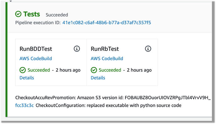
In the smoke test, the team may run both unit tests and functional tests. Ideally, these tests are better to run in parallel to speed up the pipeline. In AWS CodePipeline, we can set up a stage to run multiple steps in parallel. In our example, the pipeline runs both BDD tests and Robot Framework (RPA) tests.

The following CloudFormation code snippet runs two different tests. You use the same RunOrder value to indicate the actions run in parallel.

#...
        - Name: Tests
          Actions:
            - Name: RunBDDTest
              ActionTypeId:
                Category: Build
                Owner: AWS
                Provider: CodeBuild
                Version: 1
              Configuration:
                ProjectName: !Ref BddTestBankDemoStage
                PrimarySource: Config
              InputArtifacts:
                - Name: DemoBin
                - Name: Config
              RunOrder: 1
            - Name: RunRbTest
              ActionTypeId:
                Category: Build
                Owner: AWS
                Provider: CodeBuild
                Version: 1
              Configuration:
                ProjectName : !Ref RpaTestBankDemoStage
                PrimarySource: Config
              InputArtifacts:
                - Name: DemoBin
                - Name: Config
              RunOrder: 1  
#...

The following screenshot shows the example actions on the CodePipeline console that use the preceding code.

Screenshot of CodePipeine parallel execution tests using a same run order value

Figure – Screenshot of CodePipeine parallel execution tests

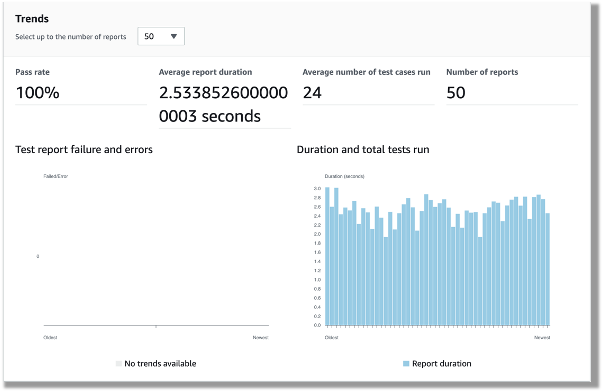
Both DBB and RPA tests produce jUnit format reports, which CodeBuild can ingest and show on the CodeBuild console. This is a great way for project management and business users to track the quality trend of an application. The following screenshot shows the CodeBuild report generated from the BDD tests.

CodeBuild report generated from the BDD tests showing 100% pass rate

Figure – CodeBuild report generated from the BDD tests

Automated regression tests

After you test the changes in the project team pipeline, you can automatically promote them to another stream with other team members’ changes for further testing. The scope of this testing stream is significantly more comprehensive, with a greater number and wider range of tests and higher volume of test data. The changes promoted to this stream by each team member are tested in this environment at the end of each day throughout the life of the project. This provides a high-quality delivery to production, with new code and changes to existing code tested together with hundreds or thousands of tests.

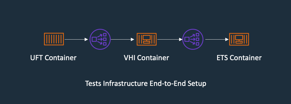
In enterprise architecture, it’s commonplace to see an application client consuming web services APIs exposed from a mainframe CICS application. One approach to do regression tests for mainframe applications is to use Micro Focus Verastream Host Integrator (VHI) to record and capture 3270 data stream processing and encapsulate these 3270 data streams as business functions, which in turn are packaged as web services. When these web services are available, they can be consumed by a test automation product, which in our environment is Micro Focus UFT One. This uses the Verastream server as the orchestration engine that translates the web service requests into 3270 data streams that integrate with the mainframe CICS application. The application is deployed in Micro Focus Enterprise Test Server.

The following diagram shows the end-to-end testing components.

Regression Test the end-to-end testing components using ECS Container for Exterprise Test Server, Verastream Host Integrator and UFT One Container, all integration points are using Elastic Network Load Balancer

Figure – Regression Test Infrastructure end-to-end Setup

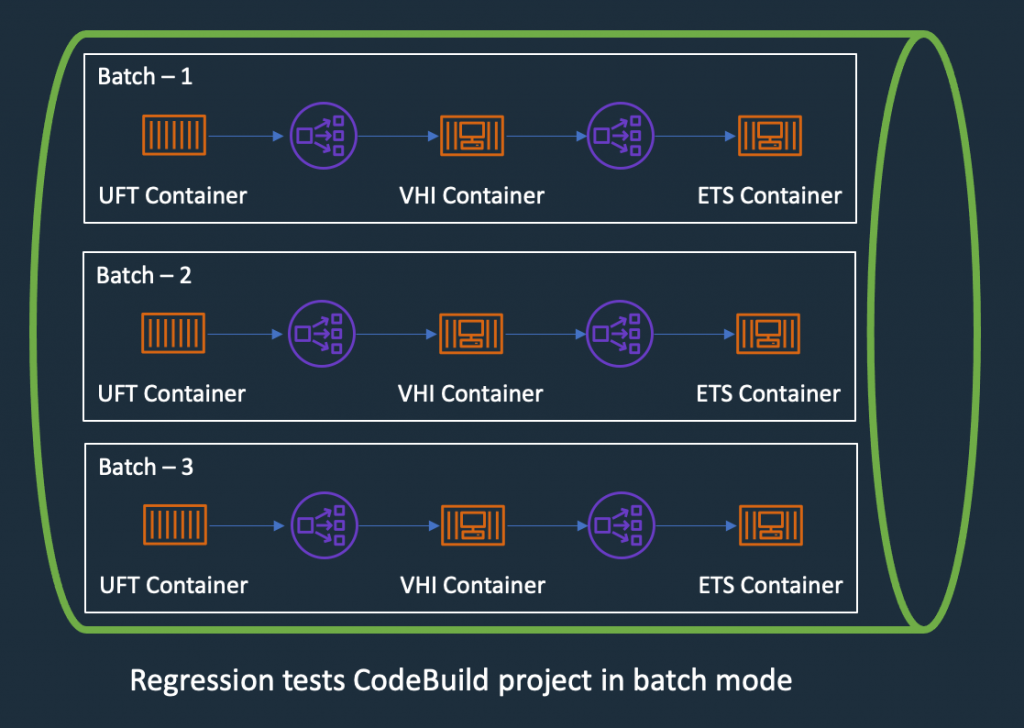
To ensure we have the coverage required for large mainframe applications, we sometimes need to run thousands of tests against very large production volumes of test data. We want the tests to run faster and complete as soon as possible so we reduce AWS costs—we only pay for the infrastructure when consuming resources for the life of the test environment when provisioning and running tests.

Therefore, the design of the test environment needs to scale out. The batch feature in CodeBuild allows you to run tests in batches and in parallel rather than serially. Furthermore, our solution needs to minimize interference between batches, a failure in one batch doesn’t affect another running in parallel. The following diagram depicts the high-level design, with each batch build running in its own independent infrastructure. Each infrastructure is launched as part of test preparation, and then torn down in the post-test phase.

Regression Tests in CodeBuoild Project setup to use batch mode, three batches running in independent infrastructure with containers

Figure – Regression Tests in CodeBuoild Project setup to use batch mode

Building and deploying regression test components

Following the design of the parallel regression test environment, let’s look at how we build each component and how they are deployed. The followings steps to build our regression tests use a working backward approach, starting from deployment in the Enterprise Test Server:

  1. Create a batch build in CodeBuild.
  2. Deploy to Enterprise Test Server.
  3. Deploy the VHI model.
  4. Deploy UFT One Tests.
  5. Integrate UFT One into CodeBuild and CodePipeline and test the application.

Creating a batch build in CodeBuild

We update two components to enable a batch build. First, in the CodePipeline CloudFormation resource, we set BatchEnabled to be true for the test stage. The UFT One test preparation stage uses the CloudFormation template to create the test infrastructure. The following code is an example of the AWS CloudFormation snippet with batch build enabled:

#...
        - Name: SystemsTest
          Actions:
            - Name: Uft-Tests
              ActionTypeId:
                Category: Build
                Owner: AWS
                Provider: CodeBuild
                Version: 1
              Configuration:
                ProjectName : !Ref UftTestBankDemoProject
                PrimarySource: Config
                BatchEnabled: true
                CombineArtifacts: true
              InputArtifacts:
                - Name: Config
                - Name: DemoSrc
              OutputArtifacts:
                - Name: TestReport                
              RunOrder: 1
#...

Second, in the buildspec configuration of the test stage, we provide a build matrix setting. We use the custom environment variable TEST_BATCH_NUMBER to indicate which set of tests runs in each batch. See the following code:

version: 0.2
batch:
  fast-fail: true
  build-matrix:
    static:
      ignore-failure: false
    dynamic:
      env:
        variables:
          TEST_BATCH_NUMBER:
            - 1
            - 2
            - 3 
phases:
  pre_build:
commands:
#...

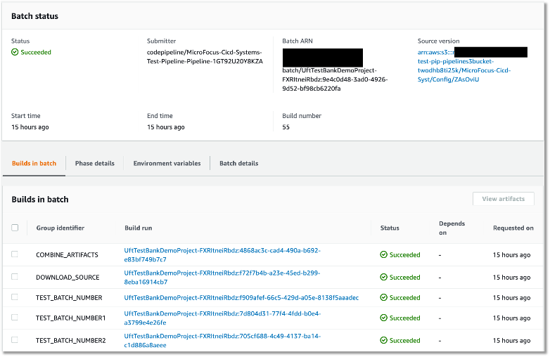
After setting up the batch build, CodeBuild creates multiple batches when the build starts. The following screenshot shows the batches on the CodeBuild console.

Regression tests Codebuild project ran in batch mode, three batches ran in prallel successfully

Figure – Regression tests Codebuild project ran in batch mode

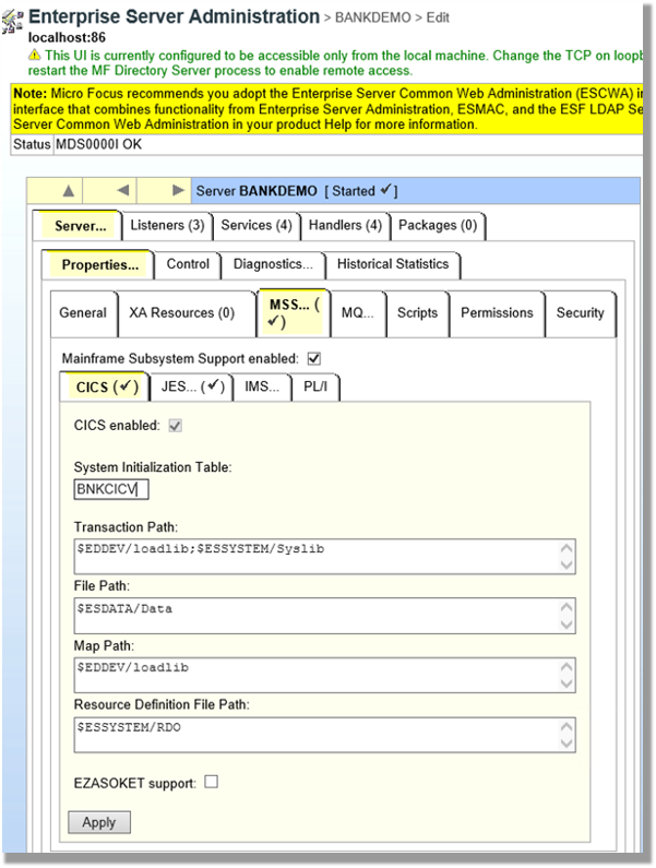
Deploying to Enterprise Test Server

ETS is the transaction engine that processes all the online (and batch) requests that are initiated through external clients, such as 3270 terminals, web services, and websphere MQ. This engine provides support for various mainframe subsystems, such as CICS, IMS TM and JES, as well as code-level support for COBOL and PL/I. The following screenshot shows the Enterprise Test Server administration page.

Enterprise Server Administrator window showing configuration for CICS

Figure – Enterprise Server Administrator window

In this mainframe application testing use case, the regression tests are CICS transactions, initiated from 3270 requests (encapsulated in a web service). For more information about Enterprise Test Server, see the Enterprise Test Server and Micro Focus websites.

In the regression pipeline, after the stage of mainframe artifact compiling, we bake in the artifact into an ETS Docker container and upload the image to an Amazon ECR repository. This way, we have an immutable artifact for all the tests.

During each batch’s test preparation stage, a CloudFormation stack is deployed to create an Amazon ECS service on Windows EC2. The stack uses a Network Load Balancer as an integration point for the VHI’s integration.

The following code is an example of the CloudFormation snippet to create an Amazon ECS service using an Enterprise Test Server Docker image:

#...
  EtsService:
    DependsOn:
    - EtsTaskDefinition
    - EtsContainerSecurityGroup
    - EtsLoadBalancerListener
    Properties:
      Cluster: !Ref 'WindowsEcsClusterArn'
      DesiredCount: 1
      LoadBalancers:
        -
          ContainerName: !Sub "ets-${AWS::StackName}"
          ContainerPort: 9270
          TargetGroupArn: !Ref EtsPort9270TargetGroup
      HealthCheckGracePeriodSeconds: 300          
      TaskDefinition: !Ref 'EtsTaskDefinition'
    Type: "AWS::ECS::Service"

  EtsTaskDefinition:
    Properties:
      ContainerDefinitions:
        -
          Image: !Sub "${AWS::AccountId}.dkr.ecr.us-east-1.amazonaws.com/systems-test/ets:latest"
          LogConfiguration:
            LogDriver: awslogs
            Options:
              awslogs-group: !Ref 'SystemsTestLogGroup'
              awslogs-region: !Ref 'AWS::Region'
              awslogs-stream-prefix: ets
          Name: !Sub "ets-${AWS::StackName}"
          cpu: 4096
          memory: 8192
          PortMappings:
            -
              ContainerPort: 9270
          EntryPoint:
          - "powershell.exe"
          Command: 
          - '-F'
          - .\StartAndWait.ps1
          - 'bankdemo'
          - C:\bankdemo\
          - 'wait'
      Family: systems-test-ets
    Type: "AWS::ECS::TaskDefinition"
#...

Deploying the VHI model

In this architecture, the VHI is a bridge between mainframe and clients.

We use the VHI designer to capture the 3270 data streams and encapsulate the relevant data streams into a business function. We can then deliver this function as a web service that can be consumed by a test management solution, such as Micro Focus UFT One.

The following screenshot shows the setup for getCheckingDetails in VHI. Along with this procedure we can also see other procedures (eg calcCostLoan) defined that get generated as a web service. The properties associated with this procedure are available on this screen to allow for the defining of the mapping of the fields between the associated 3270 screens and exposed web service.

example of VHI designer to capture the 3270 data streams and encapsulate the relevant data streams into a business function getCheckingDetails

Figure – Setup for getCheckingDetails in VHI

The following screenshot shows the editor for this procedure and is initiated by the selection of the Procedure Editor. This screen presents the 3270 screens that are involved in the business function that will be generated as a web service.

VHI designer Procedure Editor shows the procedure

Figure – VHI designer Procedure Editor shows the procedure

After you define the required functional web services in VHI designer, the resultant model is saved and deployed into a VHI Docker image. We use this image and the associated model (from VHI designer) in the pipeline outlined in this post.

For more information about VHI, see the VHI website.

The pipeline contains two steps to deploy a VHI service. First, it installs and sets up the VHI models into a VHI Docker image, and it’s pushed into Amazon ECR. Second, a CloudFormation stack is deployed to create an Amazon ECS Fargate service, which uses the latest built Docker image. In AWS CloudFormation, the VHI ECS task definition defines an environment variable for the ETS Network Load Balancer’s DNS name. Therefore, the VHI can bootstrap and point to an ETS service. In the VHI stack, it uses a Network Load Balancer as an integration point for UFT One test integration.

The following code is an example of a ECS Task Definition CloudFormation snippet that creates a VHI service in Amazon ECS Fargate and integrates it with an ETS server:

#...
  VhiTaskDefinition:
    DependsOn:
    - EtsService
    Type: AWS::ECS::TaskDefinition
    Properties:
      Family: systems-test-vhi
      NetworkMode: awsvpc
      RequiresCompatibilities:
        - FARGATE
      ExecutionRoleArn: !Ref FargateEcsTaskExecutionRoleArn
      Cpu: 2048
      Memory: 4096
      ContainerDefinitions:
        - Cpu: 2048
          Name: !Sub "vhi-${AWS::StackName}"
          Memory: 4096
          Environment:
            - Name: esHostName 
              Value: !GetAtt EtsInternalLoadBalancer.DNSName
            - Name: esPort
              Value: 9270
          Image: !Ref "${AWS::AccountId}.dkr.ecr.us-east-1.amazonaws.com/systems-test/vhi:latest"
          PortMappings:
            - ContainerPort: 9680
          LogConfiguration:
            LogDriver: awslogs
            Options:
              awslogs-group: !Ref 'SystemsTestLogGroup'
              awslogs-region: !Ref 'AWS::Region'
              awslogs-stream-prefix: vhi

#...

Deploying UFT One Tests

UFT One is a test client that uses each of the web services created by the VHI designer to orchestrate running each of the associated business functions. Parameter data is supplied to each function, and validations are configured against the data returned. Multiple test suites are configured with different business functions with the associated data.

The following screenshot shows the test suite API_Bankdemo3, which is used in this regression test process.

the screenshot shows the test suite API_Bankdemo3 in UFT One test setup console, the API setup for getCheckingDetails

Figure – API_Bankdemo3 in UFT One Test Editor Console

For more information, see the UFT One website.

Integrating UFT One and testing the application

The last step is to integrate UFT One into CodeBuild and CodePipeline to test our mainframe application. First, we set up CodeBuild to use a UFT One container. The Docker image is available in Docker Hub. Then we author our buildspec. The buildspec has the following three phrases:

  • Setting up a UFT One license and deploying the test infrastructure
  • Starting the UFT One test suite to run regression tests
  • Tearing down the test infrastructure after tests are complete

The following code is an example of a buildspec snippet in the pre_build stage. The snippet shows the command to activate the UFT One license:

version: 0.2
batch: 
# . . .
phases:
  pre_build:
    commands:
      - |
        # Activate License
        $process = Start-Process -NoNewWindow -RedirectStandardOutput LicenseInstall.log -Wait -File 'C:\Program Files (x86)\Micro Focus\Unified Functional Testing\bin\HP.UFT.LicenseInstall.exe' -ArgumentList @('concurrent', 10600, 1, ${env:AUTOPASS_LICENSE_SERVER})        
        Get-Content -Path LicenseInstall.log
        if (Select-String -Path LicenseInstall.log -Pattern 'The installation was successful.' -Quiet) {
          Write-Host 'Licensed Successfully'
        } else {
          Write-Host 'License Failed'
          exit 1
        }
#...

The following command in the buildspec deploys the test infrastructure using the AWS Command Line Interface (AWS CLI)

aws cloudformation deploy --stack-name $stack_name `
--template-file cicd-pipeline/systems-test-pipeline/systems-test-service.yaml `
--parameter-overrides EcsCluster=$cluster_arn `
--capabilities CAPABILITY_IAM

Because ETS and VHI are both deployed with a load balancer, the build detects when the load balancers become healthy before starting the tests. The following AWS CLI commands detect the load balancer’s target group health:

$vhi_health_state = (aws elbv2 describe-target-health --target-group-arn $vhi_target_group_arn --query 'TargetHealthDescriptions[0].TargetHealth.State' --output text)
$ets_health_state = (aws elbv2 describe-target-health --target-group-arn $ets_target_group_arn --query 'TargetHealthDescriptions[0].TargetHealth.State' --output text)          

When the targets are healthy, the build moves into the build stage, and it uses the UFT One command line to start the tests. See the following code:

$process = Start-Process -Wait  -NoNewWindow -RedirectStandardOutput UFTBatchRunnerCMD.log `
-FilePath "C:\Program Files (x86)\Micro Focus\Unified Functional Testing\bin\UFTBatchRunnerCMD.exe" `
-ArgumentList @("-source", "${env:CODEBUILD_SRC_DIR_DemoSrc}\bankdemo\tests\API_Bankdemo\API_Bankdemo${env:TEST_BATCH_NUMBER}")

The next release of Micro Focus UFT One (November or December 2020) will provide an exit status to indicate a test’s success or failure.

When the tests are complete, the post_build stage tears down the test infrastructure. The following AWS CLI command tears down the CloudFormation stack:


#...
	post_build:
	  finally:
	  	- |
		  Write-Host "Clean up ETS, VHI Stack"
		  #...
		  aws cloudformation delete-stack --stack-name $stack_name
          aws cloudformation wait stack-delete-complete --stack-name $stack_name

At the end of the build, the buildspec is set up to upload UFT One test reports as an artifact into Amazon Simple Storage Service (Amazon S3). The following screenshot is the example of a test report in HTML format generated by UFT One in CodeBuild and CodePipeline.

UFT One HTML report shows regression testresult and test detals

Figure – UFT One HTML report

A new release of Micro Focus UFT One will provide test report formats supported by CodeBuild test report groups.

Conclusion

In this post, we introduced the solution to use Micro Focus Enterprise Suite, Micro Focus UFT One, Micro Focus VHI, AWS developer tools, and Amazon ECS containers to automate provisioning and running mainframe application tests in AWS at scale.

The on-demand model allows you to create the same test capacity infrastructure in minutes at a fraction of your current on-premises mainframe cost. It also significantly increases your testing and delivery capacity to increase quality and reduce production downtime.

A demo of the solution is available in AWS Partner Micro Focus website AWS Mainframe CI/CD Enterprise Solution. If you’re interested in modernizing your mainframe applications, please visit Micro Focus and contact AWS mainframe business development at [email protected].

References

Micro Focus


Peter Woods

Peter Woods

Peter has been with Micro Focus for almost 30 years, in a variety of roles and geographies including Technical Support, Channel Sales, Product Management, Strategic Alliances Management and Pre-Sales, primarily based in Europe but for the last four years in Australia and New Zealand. In his current role as Pre-Sales Manager, Peter is charged with driving and supporting sales activity within the Application Modernization and Connectivity team, based in Melbourne.

Leo Ervin

Leo Ervin

Leo Ervin is a Senior Solutions Architect working with Micro Focus Enterprise Solutions working with the ANZ team. After completing a Mathematics degree Leo started as a PL/1 programming with a local insurance company. The next step in Leo’s career involved consulting work in PL/1 and COBOL before he joined a start-up company as a technical director and partner. This company became the first distributor of Micro Focus software in the ANZ region in 1986. Leo’s involvement with Micro Focus technology has continued from this distributorship through to today with his current focus on cloud strategies for both DevOps and re-platform implementations.

Kevin Yung

Kevin Yung

Kevin is a Senior Modernization Architect in AWS Professional Services Global Mainframe and Midrange Modernization (GM3) team. Kevin currently is focusing on leading and delivering mainframe and midrange applications modernization for large enterprise customers.

Architecting a Data Lake for Higher Education Student Analytics

Post Syndicated from Craig Jordan original https://aws.amazon.com/blogs/architecture/architecting-data-lake-for-higher-education-student-analytics/

One of the keys to identifying timely and impactful actions is having enough raw material to work with. However, this up-to-date information typically lives in the databases that sit behind several different applications. One of the first steps to finding data-driven insights is gathering that information into a single store that an analyst can use without interfering with those applications.

For years, reporting environments have relied on a data warehouse stored in a single, separate relational database management system (RDBMS). But now, due to the growing use of Software as a service (SaaS) applications and NoSQL database options, data may be stored outside the data center and in formats other than tables of rows and columns. It’s increasingly difficult to access the data these applications maintain, and a data warehouse may not be flexible enough to house the gathered information.

For these reasons, reporting teams are building data lakes, and those responsible for using data analytics at universities and colleges are no different. However, it can be challenging to know exactly how to start building this expanded data repository so it can be ready to use quickly and still expandable as future requirements are uncovered. Helping higher education institutions address these challenges is the topic of this post.

About Maryville University

Maryville University is a nationally recognized private institution located in St. Louis, Missouri, and was recently named the second fastest growing private university by The Chronicle of Higher Education. Even with its enrollment growth, the university is committed to a highly personalized education for each student, which requires reliable data that is readily available to multiple departments. University leaders want to offer the right help at the right time to students who may be having difficulty completing the first semester of their course of study. To get started, the data experts in the Office of Strategic Information and members of the IT Department needed to create a data environment to identify students needing assistance.

Critical data sources

Like most universities, Maryville’s student-related data centers around two significant sources: the student information system (SIS), which houses student profiles, course completion, and financial aid information; and the learning management system (LMS) in which students review course materials, complete assignments, and engage in online discussions with faculty and fellow students.

The first of these, the SIS, stores its data in an on-premises relational database, and for several years, a significant subset of its contents had been incorporated into the university’s data warehouse. The LMS, however, contains data that the team had not tried to bring into their data warehouse. Moreover, that data is managed by a SaaS application from Instructure, called “Canvas,” and is not directly accessible for traditional extract, transform, and load (ETL) processing. The team recognized they needed a new approach and began down the path of creating a data lake in AWS to support their analysis goals.

Getting started on the data lake

The first step the team took in building their data lake made use of an open source solution that Harvard’s IT department developed. The solution, comprised of AWS Lambda functions and Amazon Simple Storage Service (S3) buckets, is deployed using AWS CloudFormation. It enables any university that uses Canvas for their LMS to implement a solution that moves LMS data into an S3 data lake on a daily basis. The following diagram illustrates this portion of Maryville’s data lake architecture:

The data lake for the Learning Management System data

Diagram 1: The data lake for the Learning Management System data

The AWS Lambda functions invoke the LMS REST API on a daily schedule resulting in Maryville’s data, which has been previously unloaded and compressed by Canvas, to be securely stored into S3 objects. AWS Glue tables are defined to provide access to these S3 objects. Amazon Simple Notification Service (SNS) informs stakeholders the status of the data loads.

Expanding the data lake

The next step was deciding how to copy the SIS data into S3. The team decided to use the AWS Database Migration Service (DMS) to create daily snapshots of more than 2,500 tables from this database. DMS uses a source endpoint for secure access to the on-premises database instance over VPN. A target endpoint determines the specific S3 bucket into which the data should be written. A migration task defines which tables to copy from the source database along with other migration options. Finally, a replication instance, a fully managed virtual machine, runs the migration task to copy the data. With this configuration in place, the data lake architecture for SIS data looks like this:

Diagram 2: Migrating data from the Student Information System

Diagram 2: Migrating data from the Student Information System

Handling sensitive data

In building a data lake you have several options for handling sensitive data including:

  • Leaving it behind in the source system and avoid copying it through the data replication process
  • Copying it into the data lake, but taking precautions to ensure that access to it is limited to authorized staff
  • Copying it into the data lake, but applying processes to eliminate, mask, or otherwise obfuscate the data before it is made accessible to analysts and data scientists

The Maryville team decided to take the first of these approaches. Building the data lake gave them a natural opportunity to assess where this data was stored in the source system and then make changes to the source database itself to limit the number of highly sensitive data fields.

Validating the data lake

With these steps completed, the team turned to the final task, which was to validate the data lake. For this process they chose to make use of Amazon Athena, AWS Glue, and Amazon Redshift. AWS Glue provided multiple capabilities including metadata extraction, ETL, and data orchestration. Metadata extraction, completed by Glue crawlers, quickly converted the information that DMS wrote to S3 into metadata defined in the Glue data catalog. This enabled the data in S3 to be accessed using standard SQL statements interactively in Athena. Without the added cost and complexity of a database, Maryville’s data analyst was able to confirm that the data loads were completing successfully. He was also able to resolve specific issues encountered on particular tables. The SQL queries, written in Athena, could later be converted to ETL jobs in AWS Glue, where they could be triggered on a schedule to create additional data in S3. Athena and Glue enabled the ETL that was needed to transform the raw data delivered to S3 into prepared datasets necessary for existing dashboards.

Once curated datasets were created and stored in S3, the data was loaded into an AWS Redshift data warehouse, which supported direct access by tools outside of AWS using ODBC/JDBC drivers. This capability enabled Maryville’s team to further validate the data by attaching the data in Redshift to existing dashboards that were running in Maryville’s own data center. Redshift’s stored procedure language allowed the team to port some key ETL logic so that the engineering of these datasets could follow a process similar to approaches used in Maryville’s on-premises data warehouse environment.

Conclusion

The overall data lake/data warehouse architecture that the Maryville team constructed currently looks like this:

The complete architecture

Diagram 3: The complete architecture

Through this approach, Maryville’s two-person team has moved key data into position for use in a variety of workloads. The data in S3 is now readily accessible for ad hoc interactive SQL workloads in Athena, ETL jobs in Glue, and ultimately for machine learning workloads running in EC2, Lambda or Amazon Sagemaker. In addition, the S3 storage layer is easy to expand without interrupting prior workloads. At the time of this writing, the Maryville team is both beginning to use this environment for machine learning models described earlier as well as adding other data sources into the S3 layer.

Acknowledgements

The solution described in this post resulted from the collaborative effort of Christine McQuie, Data Engineer, and Josh Tepen, Cloud Engineer, at Maryville University, with guidance from Travis Berkley and Craig Jordan, AWS Solutions Architects.

Unified serverless streaming ETL architecture with Amazon Kinesis Data Analytics

Post Syndicated from Ram Vittal original https://aws.amazon.com/blogs/big-data/unified-serverless-streaming-etl-architecture-with-amazon-kinesis-data-analytics/

Businesses across the world are seeing a massive influx of data at an enormous pace through multiple channels. With the advent of cloud computing, many companies are realizing the benefits of getting their data into the cloud to gain meaningful insights and save costs on data processing and storage. As businesses embark on their journey towards cloud solutions, they often come across challenges involving building serverless, streaming, real-time ETL (extract, transform, load) architecture that enables them to extract events from multiple streaming sources, correlate those streaming events, perform enrichments, run streaming analytics, and build data lakes from streaming events.

In this post, we discuss the concept of unified streaming ETL architecture using a generic serverless streaming architecture with Amazon Kinesis Data Analytics at the heart of the architecture for event correlation and enrichments. This solution can address a variety of streaming use cases with various input sources and output destinations. We then walk through a specific implementation of the generic serverless unified streaming architecture that you can deploy into your own AWS account for experimenting and evolving this architecture to address your business challenges.

Overview of solution

As data sources grow in volume, variety, and velocity, the management of data and event correlation become more challenging. Most of the challenges stem from data silos, in which different teams and applications manage data and events using their own tools and processes.

Modern businesses need a single, unified view of the data environment to get meaningful insights through streaming multi-joins, such as the correlation of sensory events and time-series data. Event correlation plays a vital role in automatically reducing noise and allowing the team to focus on those issues that really matter to the business objectives.

To realize this outcome, the solution proposes creating a three-stage architecture:

  • Ingestion
  • Processing
  • Analysis and visualization

The source can be a varied set of inputs comprising structured datasets like databases or raw data feeds like sensor data that can be ingested as single or multiple parallel streams. The solution envisions multiple hybrid data sources as well. After it’s ingested, the data is divided into single or multiple data streams depending on the use case and passed through a preprocessor (via an AWS Lambda function). This highly customizable processor transforms and cleanses data to be processed through analytics application. Furthermore, the architecture allows you to enrich data or validate it against standard sets of reference data, for example validating against postal codes for address data received from the source to verify its accuracy. After the data is processed, it’s sent to various sink platforms depending on your preferences, which could range from storage solutions to visualization solutions, or even stored as a dataset in a high-performance database.

The solution is designed with flexibility as a key tenant to address multiple, real-world use cases. The following diagram illustrates the solution architecture.

The architecture has the following workflow:

  1. We use AWS Database Migration Service (AWS DMS) to push records from the data source into AWS in real time or batch. For our use case, we use AWS DMS to fetch records from an on-premises relational database.
  2. AWS DMS writes records to Amazon Kinesis Data Streams. The data is split into multiple streams as necessitated through the channels.
  3. A Lambda function picks up the data stream records and preprocesses them (adding the record type). This is an optional step, depending on your use case.
  4. Processed records are sent to the Kinesis Data Analytics application for querying and correlating in-application streams, taking into account Amazon Simple Storage Service (Amazon S3) reference data for enrichment.

Solution walkthrough

For this post, we demonstrate an implementation of the unified streaming ETL architecture using Amazon RDS for MySQL as the data source and Amazon DynamoDB as the target. We use a simple order service data model that comprises orders, items, and products, where an order can have multiple items and the product is linked to an item in a reference relationship that provides detail about the item, such as description and price.

We implement a streaming serverless data pipeline that ingests orders and items as they are recorded in the source system into Kinesis Data Streams via AWS DMS. We build a Kinesis Data Analytics application that correlates orders and items along with reference product information and creates a unified and enriched record. Kinesis Data Analytics outputs output this unified and enriched data to Kinesis Data Streams. A Lambda function consumer processes the data stream and writes the unified and enriched data to DynamoDB.

To launch this solution in your AWS account, use the GitHub repo.

Prerequisites

Before you get started, make sure you have the following prerequisites:

Setting up AWS resources in your account

To set up your resources for this walkthrough, complete the following steps:

  1. Set up the AWS CDK for Java on your local workstation. For instructions, see Getting Started with the AWS CDK.
  2. Install Maven binaries for Java if you don’t have Maven installed already.
  3. If this is the first installation of the AWS CDK, make sure to run cdk bootstrap.
  4. Clone the following GitHub repo.
  5. Navigate to the project root folder and run the following commands to build and deploy:
    1. mvn compile
    2. cdk deploy UnifiedStreamETLCommonStack UnifiedStreamETLDataStack UnifiedStreamETLProcessStack

Setting up the orders data model for CDC

In this next step, you set up the orders data model for change data capture (CDC).

  1. On the Amazon Relational Database Service (Amazon RDS) console, choose Databases.
  2. Choose your database and make sure that you can connect to it securely for testing using bastion host or other mechanisms (not detailed in scope of this post).
  3. Start MySQL Workbench and connect to your database using your DB endpoint and credentials.
  4. To create the data model in your Amazon RDS for MySQL database, run orderdb-setup.sql.
  5. On the AWS DMS console, test the connections to your source and target endpoints.
  6. Choose Database migration tasks.
  7. Choose your AWS DMS task and choose Table statistics.
  8. To update your table statistics, restart the migration task (with full load) for replication.
  9. From your MySQL Workbench session, run orders-data-setup.sql to create orders and items.
  10. Verify that CDC is working by checking the Table statistics

Setting up your Kinesis Data Analytics application

To set up your Kinesis Data Analytics application, complete the following steps:

  1. Upload the product reference products.json to your S3 bucket with the logical ID prefix unifiedBucketId (which was previously created by cdk deploy).

You can now create a Kinesis Data Analytics application and map the resources to the data fields.

  1. On the Amazon Kinesis console, choose Analytics Application.
  2. Choose Create application.
  3. For Runtime, choose SQL.
  4. Connect the streaming data created using the AWS CDK as a unified order stream.
  5. Choose Discover schema and wait for it to discover the schema for the unified order stream. If discovery fails, update the records on the source Amazon RDS tables and send streaming CDC records.
  6. Save and move to the next step.
  7. Connect the reference S3 bucket you created with the AWS CDK and uploaded with the reference data.
  8. Input the following:
    1. “products.json” on the path to the S3 object
    2. Products on the in-application reference table name
  9. Discover the schema, then save and close.
  10. Choose SQL Editor and start the Kinesis Data Analytics application.
  11. Edit the schema for SOURCE_SQL_STREAM_001 and map the data resources as follows:
Column Name Column Type Row Path
orderId INTEGER $.data.orderId
itemId INTEGER $.data.orderId
itemQuantity INTEGER $.data.itemQuantity
itemAmount REAL $.data.itemAmount
itemStatus VARCHAR $.data.itemStatus
COL_timestamp VARCHAR $.metadata.timestamp
recordType VARCHAR $.metadata.table-name
operation VARCHAR $.metadata.operation
partitionkeytype VARCHAR $.metadata.partition-key-type
schemaname VARCHAR $.metadata.schema-name
tablename VARCHAR $.metadata.table-name
transactionid BIGINT $.metadata.transaction-id
orderAmount DOUBLE $.data.orderAmount
orderStatus VARCHAR $.data.orderStatus
orderDateTime TIMESTAMP $.data.orderDateTime
shipToName VARCHAR $.data.shipToName
shipToAddress VARCHAR $.data.shipToAddress
shipToCity VARCHAR $.data.shipToCity
shipToState VARCHAR $.data.shipToState
shipToZip VARCHAR $.data.shipToZip


  1. Choose Save schema and update stream samples.

When it’s complete, verify for 1 minute that nothing is in the error stream. If an error occurs, check that you defined the schema correctly.

  1. On your Kinesis Data Analytics application, choose your application and choose Real-time analytics.
  2. Go to the SQL results and run kda-orders-setup.sql to create in-application streams.
  3. From the application, choose Connect to destination.
  4. For Kinesis data stream, choose unifiedOrderEnrichedStream.
  5. For In-application stream, choose ORDER_ITEM_ENRICHED_STREAM.
  6. Choose Save and Continue.

Testing the unified streaming ETL architecture

You’re now ready to test your architecture.

  1. Navigate to your Kinesis Data Analytics application.
  2. Choose your app and choose Real-time analytics.
  3. Go to the SQL results and choose Real-time analytics.
  4. Choose the in-application stream ORDER_ITEM_ENRCIHED_STREAM to see the results of the real-time join of records from the order and order item streaming Kinesis events.
  5. On the Lambda console, search for UnifiedStreamETLProcess.
  6. Choose the function and choose Monitoring, Recent invocations.
  7. Verify the Lambda function run results.
  8. On the DynamoDB console, choose the OrderEnriched table.
  9. Verify the unified and enriched records that combine order, item, and product records.

The following screenshot shows the OrderEnriched table.

Operational aspects

When you’re ready to operationalize this architecture for your workloads, you need to consider several aspects:

  • Monitoring metrics for Kinesis Data Streams: GetRecords.IteratorAgeMilliseconds, ReadProvisionedThroughputExceeded, and WriteProvisionedThroughputExceeded
  • Monitoring metrics available for the Lambda function, including but not limited to Duration, IteratorAge, Error count and success rate (%), Concurrent executions, and Throttles
  • Monitoring metrics for Kinesis Data Analytics (millisBehindLatest)
  • Monitoring DynamoDB provisioned read and write capacity units
  • Using the DynamoDB automatic scaling feature to automatically manage throughput

We used the solution architecture with the following configuration settings to evaluate the operational performance:

  • Kinesis OrdersStream with two shards and Kinesis OrdersEnrichedStream with two shards
  • The Lambda function code does asynchronous processing with Kinesis OrdersEnrichedStream records in concurrent batches of five, with batch size as 500
  • DynamoDB provisioned WCU is 3000, RCU is 300

We observed the following results:

  • 100,000 order items are enriched with order event data and product reference data and persisted to DynamoDB
  • An average of 900 milliseconds latency from the time of event ingestion to the Kinesis pipeline to when the record landed in DynamoDB

The following screenshot shows the visualizations of these metrics.

Cleaning up

To avoid incurring future charges, delete the resources you created as part of this post (the AWS CDK provisioned AWS CloudFormation stacks).

Conclusion

In this post, we designed a unified streaming architecture that extracts events from multiple streaming sources, correlates and performs enrichments on events, and persists those events to destinations. We then reviewed a use case and walked through the code for ingesting, correlating, and consuming real-time streaming data with Amazon Kinesis, using Amazon RDS for MySQL as the source and DynamoDB as the target.

Managing an ETL pipeline through Kinesis Data Analytics provides a cost-effective unified solution to real-time and batch database migrations using common technical knowledge skills like SQL querying.


About the Authors

Ram Vittal is an enterprise solutions architect at AWS. His current focus is to help enterprise customers with their cloud adoption and optimization journey to improve their business outcomes. In his spare time, he enjoys tennis, photography, and movies.


Akash Bhatia is a Sr. solutions architect at AWS. His current focus is helping customers achieve their business outcomes through architecting and implementing innovative and resilient solutions at scale.


Modernizing and containerizing a legacy MVC .NET application with Entity Framework to .NET Core with Entity Framework Core: Part 2

Post Syndicated from Pratip Bagchi original https://aws.amazon.com/blogs/devops/modernizing-and-containerizing-a-legacy-mvc-net-application-with-entity-framework-to-net-core-with-entity-framework-core-part-2/

This is the second post in a two-part series in which you migrate and containerize a modernized enterprise application. In Part 1, we walked you through a step-by-step approach to re-architect a legacy ASP.NET MVC application and ported it to .NET Core Framework. In this post, you will deploy the previously re-architected application to Amazon Elastic Container Service (Amazon ECS) and run it as a task with AWS Fargate.

Overview of solution

In the first post, you ported the legacy MVC ASP.NET application to ASP.NET Core, you will now modernize the same application as a Docker container and host it in the ECS cluster.

The following diagram illustrates this architecture.

Architecture Diagram


You first launch a SQL Server Express RDS (1) instance and create a Cycle Store database on that instance with tables of different categories and subcategories of bikes. You use the previously re-architected and modernized ASP.NET Core application as a starting point for this post, this app is using AWS Secrets Manager (2) to fetch database credentials to access Amazon RDS instance. In the next step, you build a Docker image of the application and push it to Amazon Elastic Container Registry (Amazon ECR) (3). After this you create an ECS cluster (4) to run the Docker image as a AWS Fargate task.

Prerequisites

For this walkthrough, you should have the following prerequisites:

This post implements the solution in Region us-east-1.

Source Code

Clone the source code from the GitHub repo. The source code folder contains the re-architected source code and the AWS CloudFormation template to launch the infrastructure, and Amazon ECS task definition.

Setting up the database server

To make sure that your database works out of the box, you use a CloudFormation template to create an instance of Microsoft SQL Server Express and AWS Secrets Manager secrets to store database credentials, security groups, and IAM roles to access Amazon Relational Database Service (Amazon RDS) and Secrets Manager. This stack takes approximately 15 minutes to complete, with most of that time being when the services are being provisioned.

  1. On the AWS CloudFormation console, choose Create stack.
  2. For Prepare template, select Template is ready.
  3. For Template source, select Upload a template file.
  4. Upload SqlServerRDSFixedUidPwd.yaml, which is available in the GitHub repo.
  5. Choose Next.
    Create AWS CloudFormation stack
  6. For Stack name, enter SQLRDSEXStack.
  7. Choose Next.
  8. Keep the rest of the options at their default.
  9. Select I acknowledge that AWS CloudFormation might create IAM resources with custom names.
  10. Choose Create stack.
    Add IAM Capabilities
  11. When the status shows as CREATE_COMPLETE, choose the Outputs tab.
  12. Record the value for the SQLDatabaseEndpoint key.
    CloudFormation output
  13. Connect the database from the SQL Server Management Studio with the following credentials:User id: DBUserand Password:DBU$er2020

Setting up the CYCLE_STORE database

To set up your database, complete the following steps:

  1. On the SQL Server Management console, connect to the DB instance using the ID and password you defined earlier.
  2. Under File, choose New.
  3. Choose Query with Current Connection.Alternatively, choose New Query from the toolbar.
    Run database restore script
  4. Open CYCLE_STORE_Schema_data.sql from the GitHub repository and run it.

This creates the CYCLE_STORE database with all the tables and data you need.

Setting up the ASP.NET MVC Core application

To set up your ASP.NET application, complete the following steps:

  1. Open the re-architected application code that you cloned from the GitHub repo. The Dockerfile added to the solution enables Docker support.
  2. Open the appsettings.Development.json file and replace the RDS endpoint present in the ConnectionStrings section with the output of the AWS CloudFormation stack without the port number which is :1433 for SQL Server.

The ASP.NET application should now load with bike categories and subcategories. See the following screenshot.

Final run

Setting up Amazon ECR

To set up your repository in Amazon ECR, complete the following steps:

  1. On the Amazon ECR console, choose Repositories.
  2. Choose Create repository.
  3. For Repository name, enter coretoecsrepo.
  4. Choose Create repository Create repositiory
  5. Copy the repository URI to use later.
  6. Select the repository you just created and choose View push commands.View Push Commands
  7. In the folder where you cloned the repo, navigate to the AdventureWorksMVCCore.Web folder.
  8. In the View push commands popup window, complete steps 1–4 to push your Docker image to Amazon ECR. Push to Amazon Elastic Repository

The following screenshot shows completion of Steps 1 and 2 and ensure your working directory is set to AdventureWorksMVCCore.Web as below.

Login
The following screenshot shows completion of Steps 3 and 4.

Amazon ECR Push

Setting up Amazon ECS

To set up your ECS cluster, complete the following steps:

    1. On the Amazon ECS console, choose Clusters.
    2. Choose Create cluster.
    3. Choose the Networking only cluster template.
    4. Name your cluster cycle-store-cluster.
    5. Leave everything else as its default.
    6. Choose Create cluster.
    7. Select your cluster.
    8. Choose Task Definitions and choose Create new Task Definition.
    9. On the Select launch type compatibility page choose FARGATE and click Next step.
    10. On the Configure task and container definitions page, scroll to the bottom of the page and choose Configure via JSON.
    11. In the text area, enter the task definition JSON (task-definition.json) provided in the GitHub repo. Make sure to replace [YOUR-AWS-ACCOUNT-NO] in task-definition.json with your AWS account number on the line number 44, 68 and 71. The task definition file assumes that you named your repository as coretoecsrepo. If you named it something else, modify this file accordingly. It also assumes that you are using us-east-1 as your default region, so please consider replacing the region in the task-definition.json on line number 15 and 44 if you are not using us-east-1 region. Replace AWS Account number
    12. Choose Save.
    13. On the Task Definitions page, select cycle-store-td.
    14. From the Actions drop-down menu, choose Run Task.Run task
    15. Choose Launch type is equal to Fargate.
    16. Choose your default VPC as Cluster VPC.
    17. Select at least one Subnet.
    18. Choose Edit Security Groups and select ECSSecurityGroup (created by the AWS CloudFormation stack).Select security group
    19. Choose Run Task

Running your application

Choose the link under the task and find the public IP. When you navigate to the URL http://your-public-ip, you should see the .NET Core Cycle Store web application user interface running in Amazon ECS.

See the following screenshot.

Final run

Cleaning up

To avoid incurring future charges, delete the stacks you created for this post.

  1. On the AWS CloudFormation console, choose Stacks.
  2. Select SQLRDSEXStack.
  3. In the Stack details pane, choose Delete.

Conclusion

This post concludes your journey towards modernizing a legacy enterprise MVC ASP.NET web application using .NET Core and containerizing using Amazon ECS using the AWS Fargate compute engine on a Linux container. Portability to .NET Core helps you run enterprise workload without any dependencies on windows environment and AWS Fargate gives you a way to run containers directly without managing any EC2 instances and giving you full control. Additionally, couple of recent launched AWS tools in this area.

About the Author

Saleha Haider is a Senior Partner Solution Architect with Amazon Web Services.
Pratip Bagchi is a Partner Solutions Architect with Amazon Web Services.


Migrating Subversion repositories to AWS CodeCommit

Post Syndicated from Iftikhar khan original https://aws.amazon.com/blogs/devops/migrating-subversion-repositories-aws-codecommit/

In this post, we walk you through migrating Subversion (SVN) repositories to AWS CodeCommit. But before diving into the migration, we do a brief review of SVN and Git based systems such as CodeCommit.

About SVN

SVN is an open-source version control system. Founded in 2000 by CollabNet, Inc., it was originally designed to be a better Concurrent Versions System (CVS), and is being developed as a project of the Apache Software Foundation. SVN is the third implementation of a revision control system: Revision Control System (RCS), then CVS, and finally SVN.

SVN is the leader in centralized version control. Systems such as CVS and SVN have a single remote server of versioned data with individual users operating locally against copies of that data’s version history. Developers commit their changes directly to that central server repository.

All the files and commit history information are stored in a central server, but working on a single central server means more chances of having a single point of failure. SVN offers few offline access features; a developer has to connect to the SVN server to make a commit that makes commits slower. The single point of failure, security, maintenance, and scaling SVN infrastructure are the major concerns for any organization.

About DVCS

Distributed Version Control Systems (DVCSs) address the concerns and challenges of SVN. In a DVCS (such as Git or Mercurial), you don’t just check out the latest snapshot of the files; rather, you fully mirror the repository, including its full history. If any server dies, and these systems are collaborating via that server, you can copy any of the client repositories back up to the server to restore it. Every clone is a full backup of all the data.

DVCs such as Git are built with speed, non-linear development, simplicity, and efficiency in mind. It works very efficiently with large projects, which is one of the biggest factors why customers find it popular.

A significant reason to migrate to Git is branching and merging. Creating a branch is very lightweight, which allows you to work faster and merge easily.

About CodeCommit

CodeCommit is a version control system that is fully managed by AWS. CodeCommit can host secure and highly scalable private Git repositories, which eliminates the need to operate your source control system and scale its infrastructure. You can use it to securely store anything, from source code to binaries. CodeCommit features like collaboration, encryption, and easy access control make it a great choice. It works seamlessly with most existing Git tools and provides free private repositories.

Understanding the repository structure of SVN and Git

SVNs have a tree model with one branch where the revisions are stored, whereas Git uses a graph structure and each commit is a node that knows its parent. When comparing the two, consider the following features:

  • Trunk – An SVN trunk is like a primary branch in a Git repository, and contains tested and stable code.
  • Branches – For SVN, branches are treated as separate entities with its own history. You can merge revisions between branches, but they’re different entities. Because of its centralized nature, all branches are remote. In Git, branches are very cheap; it’s a pointer for a particular commit on the tree. It can be local or be pushed to a remote repository for collaboration.
  • Tags – A tag is just another folder in the main repository in SVN and remains static. In Git, a tag is a static pointer to a specific commit.
  • Commits – To commit in SVN, you need access to the main repository and it creates a new revision in the remote repository. On Git, the commit happens locally, so you don’t need to have access to the remote. You can commit the work locally and then push all the commits at one time.

So far, we have covered how SVN is different from Git-based version control systems and illustrated the layout of SVN repositories. Now it’s time to look at how to migrate SVN repositories to CodeCommit.

Planning for migration

Planning is always a good thing. Before starting your migration, consider the following:

  • Identify SVN branches to migrate.
  • Come up with a branching strategy for CodeCommit and document how you can map SVN branches.
  • Prepare build, test scripts, and test cases for system testing.

If the size of the SVN repository is big enough, consider running all migration commands on the SVN server. This saves time because it eliminates network bottlenecks.

Migrating the SVN repository to CodeCommit

When you’re done with the planning aspects, it’s time to start migrating your code.

Prerequisites

You must have the AWS Command Line Interface (AWS CLI) with an active account and Git installed on the machine that you’re planning to use for migration.

Listing all SVN users for an SVN repository
SVN uses a user name for each commit, whereas Git stores the real name and email address. In this step, we map SVN users to their corresponding Git names and email.

To list all the SVN users, run the following PowerShell command from the root of your local SVN checkout:

svn.exe log --quiet | ? { $_ -notlike '-*' } | % { "{0} = {0} &amp;amp;lt;{0}&amp;amp;gt;" -f ($_ -split ' \| ')[1] } | Select-Object -Unique | Out-File 'authors-transform.txt'

On a Linux based machine, run the following command from the root of your local SVN checkout:

svn log -q | awk -F '|' '/^r/ {sub("^ ", "", $2); sub(" $", "", $2); print $2" = "$2" &lt;"$2"&gt;"}' | sort -u &gt; authors-transform.txt

The authors-transform.txt file content looks like the following code:

ikhan = ikhan <ikhan>
foobar= foobar <foobar>
abob = abob <abob>

After you transform the SVN user to a Git user, it should look like the following code:

ikhan = ifti khan <[email protected]>
fbar = foo bar <[email protected]>
abob = aaron bob <[email protected]>

Importing SVN contents to a Git repository

The next step in the migration from SVN to Git is to import the contents of the SVN repository into a new Git repository. We do this with the git svn utility, which is included with most Git distributions. The conversion process can take a significant amount of time for larger repositories.

The git svn clone command transforms the trunk, branches, and tags in your SVN repository into a new Git repository. The command depends on the structure of the SVN.

git svn clone may not be available in all installations; you might consider using an AWS Cloud9 environment or using a temporary Amazon Elastic Compute Cloud (Amazon EC2) instance.

If your SVN layout is standard, use the following command:

git svn clone --stdlayout --authors-file=authors.txt  <svn-repo>/<project> <temp-dir/project>

If your SVN layout isn’t standard, you need to map the trunk, branches, and tags folder in the command as parameters:

git svn clone <svn-repo>/<project> --prefix=svn/ --no-metadata --trunk=<trunk-dir> --branches=<branches-dir>  --tags==<tags-dir>  --authors-file "authors-transform.txt" <temp-dir/project>

Creating a bare Git repository and pushing the local repository

In this step, we create a blank repository and match the default branch with the SVN’s trunk name.

To create the .gitignore file, enter the following code:

cd <temp-dir/project>
git svn show-ignore > .gitignore
git add .gitignore
git commit -m 'Adding .gitignore.'

To create the bare Git repository, enter the following code:

git init --bare <git-project-dir>\local-bare.git
cd <git-project-dir>\local-bare.git
git symbolic-ref HEAD refs/heads/trunk

To update the local bare Git repository, enter the following code:

cd <temp-dir/project>
git remote add bare <git-project-dir\local-bare.git>
git config remote.bare.push 'refs/remotes/*:refs/heads/*'
git push bare

You can also add tags:

cd <git-project-dir\local-bare.git>

For Windows, enter the following code:

git for-each-ref --format='%(refname)' refs/heads/tags | % { $_.Replace('refs/heads/tags/','') } | % { git tag $_ "refs/heads/tags/$_"; git branch -D "tags/$_" }

For Linux, enter the following code:

for t in $(git for-each-ref --format='%(refname:short)' refs/remotes/tags); do git tag ${t/tags\//} $t &amp;&amp; git branch -D -r $t; done

You can also add branches:

cd <git-project-dir\local-bare.git>

For Windows, enter the following code:

git for-each-ref --format='%(refname)' refs/remotes | % { $_.Replace('refs/remotes/','') } | % { git branch "$_" "refs/remotes/$_"; git branch -r -d "$_"; }

For Linux, enter the following code:

for b in $(git for-each-ref --format='%(refname:short)' refs/remotes); do git branch $b refs/remotes/$b && git branch -D -r $b; done

As a final touch-up, enter the following code:

cd <git-project-dir\local-bare.git>
git branch -m trunk master

Creating a CodeCommit repository

You can now create a CodeCommit repository with the following code (make sure that the AWS CLI is configured with your preferred Region and credentials):

aws configure
aws codecommit create-repository --repository-name MySVNRepo --repository-description "SVN Migration repository" --tags Team=Migration

You get the following output:

{
    "repositoryMetadata": {
        "repositoryName": "MySVNRepo",
        "cloneUrlSsh": "ssh://ssh://git-codecommit.us-east-2.amazonaws.com/v1/repos/MySVNRepo",
        "lastModifiedDate": 1446071622.494,
        "repositoryDescription": "SVN Migration repository",
        "cloneUrlHttp": "https://git-codecommit.us-east-2.amazonaws.com/v1/repos/MySVNRepo",
        "creationDate": 1446071622.494,
        "repositoryId": "f7579e13-b83e-4027-aaef-650c0EXAMPLE",
        "Arn": "arn:aws:codecommit:us-east-2:111111111111:MySVNRepo",
        "accountId": "111111111111"
    }
}

Pushing the code to CodeCommit

To push your code to the new CodeCommit repository, enter the following code:

cd <git-project-dir\local-bare.git>
git remote add origin https://git-codecommit.us-east-2.amazonaws.com/v1/repos/MySVNRepo
git add *

git push origin --all
git push origin --tags (Optional if tags are mapped)

Troubleshooting

When migrating SVN repositories, you might encounter a few SVN errors, which are displayed as code on the console. For more information, see Subversion client errors caused by inappropriate repository URL.

For more information about the git-svn utility, see the git-svn documentation.

Conclusion

In this post, we described the straightforward process of using the git-svn utility to migrate SVN repositories to Git or Git-based systems like CodeCommit. After you migrate an SVN repository to CodeCommit, you can use any Git-based client and start using CodeCommit as your primary version control system without worrying about securing and scaling its infrastructure.