Tag Archives: open source

Introducing workerd: the Open Source Workers runtime

Post Syndicated from Kenton Varda original https://blog.cloudflare.com/workerd-open-source-workers-runtime/
Introducing workerd: the Open Source Workers runtime

Introducing workerd: the Open Source Workers runtime

Today I’m proud to introduce the first beta release of workerd, the JavaScript/Wasm runtime based on the same code that powers Cloudflare Workers. workerd is Open Source under the Apache License version 2.0.

workerd shares most of its code with the runtime that powers Cloudflare Workers, but with some changes designed to make it more portable to other environments. The name “workerd” (pronounced “worker dee”) comes from the Unix tradition of naming servers with a “-d” suffix standing for “daemon”. The name is not capitalized because it is a program name, which are traditionally lower-case in Unix-like environments.

What it’s for

Self-hosting Workers

workerd can be used to self-host applications that you’d otherwise run on Cloudflare Workers. It is intended to be a production-ready web server for this purpose. workerd has been designed to be unopinionated about hosting environments, so that it should fit nicely into whatever server/VM/container hosting and orchestration system you prefer. It’s just a web server.

Workers has always been based on standardized APIs, so that code is not locked into Cloudflare, and we work closely with other runtimes to promote compatibility. workerd provides another option to ensure that applications built on Workers can run anywhere, by leveraging the same underlying code to get exact, “bug-for-bug” compatibility.

Local development and testing

workerd is also designed to facilitate realistic local testing of Workers. Up until now, this has been achieved using Miniflare, which simulated the Workers API within a Node.js environment. Miniflare has worked well, but in a number of cases its behavior did not exactly match Workers running on Cloudflare. With the release of workerd, Miniflare and the Wrangler CLI tool will now be able to provide a more accurate simulation by leveraging the same runtime code we use in production.

Programmable proxies

workerd can act as an application host, a proxy, or both. It supports both forward and reverse proxy modes. In all cases, JavaScript code can be used to intercept and process requests and responses before forwarding them on. Traditional web servers and proxies have used bespoke configuration languages with quirks that are hard to master. Programming proxies in JavaScript instead provides more power while making the configuration easier to write and understand.

What it is

workerd is not just another way to run JavaScript and Wasm. Our runtime is uniquely designed in a number of ways.

Server-first

Many non-browser JavaScript and Wasm runtimes are designed to be general-purpose: you can use them to build command-line apps, local GUI apps, servers, or anything in between. workerd is not. It specifically focuses on servers, in particular (for now, at least) HTTP servers.

This means in particular that workerd-based applications are event-driven at the top level. Applications do not open listen sockets and accept connections from them; instead, the runtime pushes events to the application. It may seem like a minor difference, but this basic change in perspective directly enables many of the features below.

Web standard APIs

Wherever possible, Workers (and workerd in particular) offers the same standard APIs found in web browsers, such as Fetch, URL, WebCrypto, and others. This means that code built on workerd is more likely to be portable to browsers as well as to other standards-based runtimes. When Workers launched five years ago, it was unusual for a non-browser to offer web APIs, but we are pleased to see that the broader JavaScript ecosystem is now converging on them.

Nanoservices

workerd is a nanoservice runtime. What does that mean?

Microservices have become popular over the last decade as a way to split monolithic servers into smaller components that could be maintained and deployed independently. For example, a company that offers several web applications with a common user authentication flow might have a separate team that maintains the authentication logic. In a monolithic model, the authentication logic might have been offered to the application teams as a library. However, this could be frustrating for the maintainers of that logic, as making any change might require waiting for every application team to deploy an update to their respective server. By splitting the authentication logic into a separate server that all the others talk to, the authentication team is able to deploy changes on their own schedule.

However, microservices have a cost. What was previously a fast library call instead now requires communicating over a network. In addition to added overhead, this communication requires configuration and administration to ensure security and reliability. These costs become greater as the codebase is split into more and more services. Eventually, the costs outweigh the benefits.

Nanoservices are a new model that achieve the benefits of independent deployment with overhead closer to that of library calls. With workerd, many Workers can be configured to run in the same process. Each Worker runs in a separate “isolate”, which gives the appearance of running independently of the others: each isolate loads separate code and has its own global scope. However, when one Worker explicitly sends a request to another Worker, the destination Worker actually runs in the same thread with zero latency. So, it performs more like a function call.

With nanoservices, teams can now break their code into many more independently-deployed pieces without worrying about the overhead.

(Some in the industry prefer to call nanoservices “functions”, implying that each individual function making up an application could be its own service. I feel, however, that this puts too much emphasis on syntax rather than logical functionality. That said, it is the same concept.)

To really make nanoservices work well, we had to minimize the baseline overhead of each service. This required designing workerd very differently from most other runtimes, so that common resources could be shared between services as much as possible. First, as mentioned, we run many nanoservices within a single process, to share basic process overhead and minimize context switching costs. A second big architectural difference between workerd and other runtimes is how it handles built-in APIs. Many runtimes implement significant portions of their built-in APIs in JavaScript, which must then be loaded separately into each isolate. workerd does not; all the APIs are implemented in native code, so that all isolates may share the same copy of that code. These design choices would be difficult to retrofit into another runtime, and indeed these needs are exactly why we chose to build a custom runtime for Workers from the start.

Homogeneous deployment

In a typical microservices model, you might deploy different microservices to containers running across a cluster of machines, connected over a local network. You might manually choose how many containers to dedicate to each service, or you might configure some form of auto-scaling based on resource usage.

workerd offers an alternative model: Every machine runs every service.

workerd’s nanoservices are much lighter-weight than typical containers. As a result, it’s entirely reasonable to run a very large number of them – hundreds, maybe thousands – on a single server. This in turn means that you can simply deploy every service to every machine in your fleet.

Homogeneous deployment means that you don’t have to worry about scaling individual services. Instead, you can simply load balance requests across the entire cluster, and scale the cluster as needed. Overall, this can greatly reduce the amount of administration work needed.

Cloudflare itself has used the homogeneous model on our network since the beginning. Every one of Cloudflare’s edge servers runs our entire software stack, so any server can answer any kind of request on its own. We’ve found it works incredibly well. This is why services on Cloudflare – including ones that use Workers – are able to go from no traffic at all to millions of requests per second instantly without trouble.

Capability bindings: cleaner configuration and SSRF safety

workerd takes a different approach to most runtimes – indeed, to most software development platforms – in how an application accesses external resources.

Most development platforms start from assuming that the application can talk to the whole world. It is up to the application to figure out exactly what it wants to talk to, and name it in some global namespace, such as using a URL. So, an application server that wants to talk to the authentication microservice might use code like this:

// Traditional approach without capability bindings.
fetch("https://auth-service.internal-network.example.com/api", {
  method: "POST",
  body: JSON.stringify(authRequest),
  headers: { "Authorization": env.AUTH_SERVICE_TOKEN }
});

In workerd, we do things differently. An application starts out with no ability to talk to the rest of the world, and must be configured with specific capability bindings that provide it access to specific external resources. So, an application which needs to be able to talk to the authentication service would be configured with a binding called authService, and the code would look something like this:

// Capability-based approach. Hostname doesn't matter; all
// requests to AUTH_SERVICE.fetch() go to the auth service.
env.AUTH_SERVICE.fetch("https://auth/api", {
 method: "POST",
 body: JSON.stringify(authRequest),
});

This may at first appear to be a trivial difference. In both cases, we have to use configuration to control access to external services. In the traditional approach, we’d provide access tokens (and probably the service’s hostname) as environment variables. In the new approach, the environment goes a bit further to provide a full-fledged object. Is this just syntax sugar?

It turns out, this slight change has huge advantages:

First, we can now restrict the global fetch() function to accept only publicly-routable URLs. This makes applications totally immune to SSRF attacks! You cannot trick an application into accessing an internal service unintentionally if the code to access internal services is explicitly different. (In fact, the global fetch() is itself backed by a binding, which can be configured. workerd defaults to connecting it to the public internet, but you can also override it to permit private addresses if you want, or to route to a specific proxy service, or to be blocked entirely.)

With that done, we now have an interesting property: All internal services which an application uses must be configurable. This means:

  • You can easily see a complete list of the internal services an application talks to, without reading all the code.
  • You can always replace these services with mocks for testing purposes.
  • You can always configure an application to authenticate itself differently (e.g. client certificates) or use a different back end, without changing code.

The receiving end of a binding benefits, too. Take the authentication service example, above. The auth service may be another Worker running in workerd as a nanoservice. In this case, the auth service does not need to be bound to any actual network address. Instead, it may be made available strictly to other Workers through their bindings. In this case, the authentication service doesn’t necessarily need to verify that a request received came from an allowed client – because only allowed clients are able to send requests to it in the first place.

Overall, capability bindings allow simpler code that is secure by default, more composable, easier to test, and easier to understand and maintain.

Always backwards compatible

Cloudflare Workers has a hard rule against ever breaking a live Worker running in production. This same dedication to backwards compatibility extends to workerd.

workerd shares Workers’ compatibility date system to manage breaking changes. Every Worker must be configured with a “compatibility date”. The runtime then ensures that the API behaves exactly as it did on that date. At your leisure, you may check the documentation to see if new breaking changes are introduced at a future date, and update your code for them. Most such changes are minor and most code won’t require any changes. However, you are never obliged to update. Old dates will continue to be supported by newer versions of workerd. It is always safe to update workerd itself without updating your code.

What it’s not

To avoid misleading or disappointing anyone, I need to take a moment to call out what workerd is not.

workerd is not a Secure Sandbox

It’s important to note that workerd is not, on its own, a secure way to run possibly-malicious code. If you wish to run code you don’t trust using workerd, you must enclose it in an additional sandboxing layer, such as a virtual machine configured for sandboxing.

workerd itself is designed such that a Worker should not be able to access any external resources to which it hasn’t been granted a capability. However, a complete sandbox solution not only must be designed to restrict access, but also must account for the possibility of bugs – both in software and in hardware. workerd on its own is not sufficient to protect against hardware bugs like Spectre, nor can it adequately defend against the possibility of vulnerabilities in V8 or in workerd’s own code.

The Cloudflare Workers service uses the same code found in workerd, but adds many additional layers of security on top to harden against such bugs. I described some of these in a past blog post. However, these measures are closely tied to our particular environment. For example, we rely on build automation to push V8 patches to production immediately upon becoming available; we separate customers according to risk profile; we rely on non-portable kernel features and assumptions about the host system to enforce security and resource limits. All of this is very specific to our environment, and cannot be packaged up in a reusable way.

workerd is not an independent project

workerd is the core of Cloudflare Workers, a fast-moving project developed by a dedicated team at Cloudflare. We are not throwing code over the wall to forget about, nor are we expecting volunteers to do our jobs for us. workerd’s GitHub repository will be the canonical source used by Cloudflare Workers and our team will be doing much of their work directly in this repository. Just like V8 is developed primarily by the Chrome team for use in Chrome, workerd will be developed primarily by the Cloudflare Workers team for use in Cloudflare Workers.

This means we cannot promise that external contributions will sit on a level playing field with internal ones. Code reviews take time, and work that is needed for Cloudflare Workers will take priority. We also cannot promise we will accept every feature contribution. Even if the code is already written, reviews and maintenance have a cost. Within Cloudflare, we have a product management team who carefully evaluates what features we should and shouldn’t offer, and plenty of ideas generated internally ultimately don’t make the cut.

If you want to contribute a big new feature to workerd, your best bet is to talk to us before you write code, by raising an issue on GitHub early to get input. That way, you can find out if we’re likely to accept a PR before you write it. We also might be able to give hints on how best to implement.

It’s also important to note that while workerd’s internal interfaces may sometimes appear clean and reusable, we cannot make any guarantee that those interfaces won’t completely change on a whim. If you are trying to build on top of workerd internals, you will need to be prepared either to accept a fair amount of churn, or pin to a specific version.

workerd is not an off-the-shelf edge compute platform

As hinted above, the full Cloudflare Workers service involves a lot of technology beyond workerd itself, including additional security, deployment mechanisms, orchestration, and so much more. workerd itself is a portion of our runtime codebase, which is itself a small (albeit critical) piece of the overall Cloudflare Workers service.

We are pleased, though, that this means it is possible for us to release this code under a permissive Open Source license.

Try the Beta

As of this blog post, workerd is in beta. If you want to try it out,
Choose the k-NN algorithm for your billion-scale use case with OpenSearch

Post Syndicated from Jack Mazanec original https://aws.amazon.com/blogs/big-data/choose-the-k-nn-algorithm-for-your-billion-scale-use-case-with-opensearch/

When organizations set out to build machine learning (ML) applications such as natural language processing (NLP) systems, recommendation engines, or search-based systems, often times k-Nearest Neighbor (k-NN) search will be used at some point in the workflow. As the number of data points reaches the hundreds of millions or even billions, scaling a k-NN search system can be a major challenge. Applying Approximate Nearest Neighbor (ANN) search is a great way to overcome this challenge.

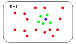
The k-NN problem is relatively simple compared to other ML techniques: given a set of points and a query, find the k nearest points in the set to the query. The naive solution is equally understandable: for each point in the set, compute its distance from the query and keep track of the top k along the way.

K-NN concept

The problem with this naive approach is that it doesn’t scale particularly well. The runtime search complexity is O(Nlogk), where N is the number of vectors and k is the number of nearest neighbors. Although this may not be noticeable when the set contains thousands of points, it becomes noticeable when the size gets into the millions. Although some exact k-NN algorithms can speed search up, they tend to perform similarly to the naive approach in higher dimensions.

Enter ANN search. We can reduce the runtime search latency if we loosen a few constraints on the k-NN problem:

  • Allow indexing to take longer
  • Allow more space to be used at query time
  • Allow the search to return an approximation of the k-NN in the set

Several different algorithms have been discovered to do just that.

OpenSearch is a community-driven, Apache 2.0-licensed, open-source search and analytics suite that makes it easy to ingest, search, visualize, and analyze data. The OpenSearch k-NN plugin provides the ability to use some of these algorithms within an OpenSearch cluster. In this post, we discuss the different algorithms that are supported and run experiments to see some of the trade-offs between them.

Hierarchical Navigable Small Worlds algorithm

The Hierarchical Navigable Small Worlds algorithm (HNSW) is one of the most popular algorithms out there for ANN search. It was the first algorithm that the k-NN plugin supported, using a very efficient implementation from the nmslib similarity search library. It has one of the best query latency vs. recall trade-offs and doesn’t require any training. The core idea of the algorithm is to build a graph with edges connecting index vectors that are close to each other. Then, on search, this graph is partially traversed to find the approximate nearest neighbors to the query vector. To steer the traversal towards the query’s nearest neighbors, the algorithm always visits the closest candidate to the query vector next.

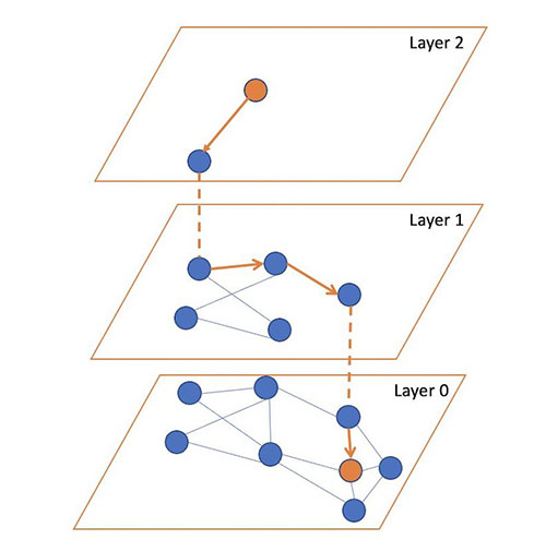
But which vector should the traversal start from? It could just pick a random vector, but for a large index, this might be very far from the query’s actual nearest neighbors, leading to poor results. To pick a vector that is generally close to the query vector to start from, the algorithm builds not just one graph, but a hierarchy of graphs. All vectors are added to the bottom layer, and then a random subset of those are added to the layer above, and then a subset of those are added to the layer above that, and so on.

During search, we start from a random vector in the top layer, partially traverse the graph to find (approximately) the nearest point to the query vector in that layer, and then use this vector as the starting point for our traversal of the layer below. We repeat this until we get to the bottom layer. At the bottom layer, we perform the traversal, but this time, instead of just searching for the nearest neighbor, we keep track of the k-nearest neighbors that are visited along the way.

The following figure illustrates this process (inspired from the image in original paper Efficient and robust approximate nearest neighbor search using Hierarchical Navigable Small World graphs).

You can tune three parameters for HNSW:

  • m – The maximum number of edges a vector will get in a graph. The higher this number is, the more memory the graph will consume, but the better the search approximation may be.
  • ef_search – The size of the queue of the candidate nodes to visit during traversal. When a node is visited, its neighbors are added to the queue to be visited in the future. When this queue is empty, the traversal will end. A larger value will increase search latency, but may provide better search approximation.
  • ef_construction – Very similar to ef_search. When a node is to be inserted into the graph, the algorithm will find its m edges by querying the graph with the new node as the query vector. This parameter controls the candidate queue size for this traversal. A larger value will increase index latency, but may provide a better search approximation.

For more information on HNSW, you can read through the paper Efficient and robust approximate nearest neighbor search using Hierarchical Navigable Small World graphs.

Memory consumption

Although HNSW provides very good approximate nearest neighbor search at low latencies, it can consume a large amount of memory. Each HNSW graph uses roughly 1.1 * (4 * d + 8 * m) * num_vectors bytes of memory:

  • d is the dimension of the vectors
  • m is the algorithm parameter that controls the number of connections each node will have in a layer
  • num_vectors is the number of vectors in the index

To ensure durability and availability, especially when running production workloads, OpenSearch indexes are recommended to have at least one replica shard. Therefore, the memory requirement is multiplied by (1 + number of replicas). For use cases where the data size is 1 billion vectors of 128 dimensions each and m is set to the default value of 16, the estimated amount of memory required would be:

1.1 * (4 * 128 + 8 * 16) * 1,000,000,000 * 2 = 1,408 GB.

If we increase the size of vectors to 512, for example, and the m to 100, which is recommended for vectors with high intrinsic dimensionality, some use cases can require a total memory of approximately 4 TB.

With OpenSearch, we can always horizontally scale the cluster to handle this memory requirement. However, this comes at the expense of raising infrastructure costs. For cases where scaling doesn’t make sense, options to reduce the memory footprint of the k-NN system need to be explored. Fortunately, there are algorithms that we can use to do this.

Inverted File System algorithm

Consider a different approach for approximating a nearest neighbor search: separate your index vectors into a set of buckets, then, to reduce your search time, only search through a subset of these buckets. From a high level, this is what the Inverted File System (IVF) ANN algorithm does. In OpenSearch 1.2, the k-NN plugin introduced support for the implementation of IVF by Faiss. Faiss is an open-sourced library from Meta for efficient similarity search and clustering of dense vectors.

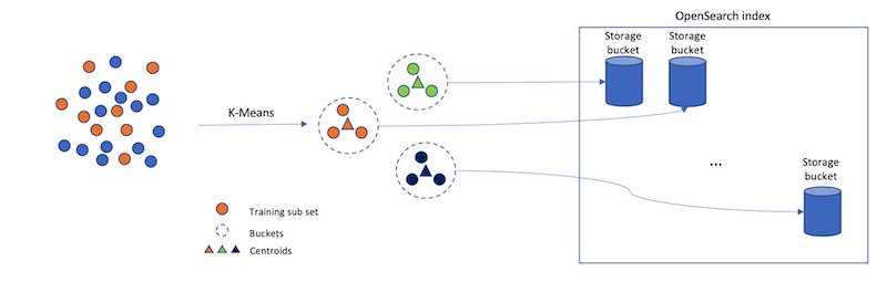
However, if we just randomly split up our vectors into different buckets, and only search a subset of them, this will be a poor approximation. The IVF algorithm uses a more elegant approach. First, before indexing begins, it assigns each bucket a representative vector. When a vector is indexed, it gets added to the bucket that has the closest representative vector. This way, vectors that are closer to each other are placed roughly in the same or nearby buckets.

To determine what the representative vectors for the buckets are, the IVF algorithm requires a training step. In this step, k-Means clustering is run on a set of training data, and the centroids it produces become the representative vectors. The following diagram illustrates this process.

Inverted file system indexing concept

IVF has two parameters:

  • nlist – The number of buckets to create. More buckets will result in longer training times, but may improve the granularity of the search.
  • nprobes – The number of buckets to search. This parameter is fairly straightforward. The more buckets that are searched, the longer the search will take, but the better the approximation.

Memory consumption

In general, IVF requires less memory than HNSW because IVF doesn’t need to store a set of edges for each indexed vector.

We estimate that IVF will roughly require the following amount of memory:

1.1 * (((4 * dimension) * num_vectors) + (4 * nlist * dimension)) bytes

For the case explored for HNSW where there are 1,000,000,000 128-dimensional vectors with one layer of replication, an IVF algorithm with an nlist of 4096 would take roughly 1.1 * (((4 * 128) * 2,000,000,000) + (4 * 4096 * 128)) bytes = 1126 GB.

This savings does come at a cost, however, because HNSW offers a better query latency versus approximation accuracy tradeoff.

Product quantization vector compression

Although you can use HNSW and IVF to speed up nearest neighbor search, they can consume a considerable amount of memory. When we get into the billion-vector scale, we start to require thousands of GBs of memory to support their index structures. As we scale up the number of vectors or the dimension of vectors, this requirement continues to grow. Is there a way to use noticeably less space for our k-NN index?

The answer is yes! In fact, there are a lot of different ways to reduce the amount of memory vectors require. You can change your embedding model to produce smaller vectors, or you can apply techniques like Principle Component Analysis (PCA) to reduce the vector’s dimensionality. Another approach is to use quantization. The general idea of vector quantization is to map a large vector space with continuous values into a smaller space with discrete values. When a vector is mapped into a smaller space, it requires fewer bits to represent. However, this comes at a cost—when mapping to a smaller input space, some information about the vector is lost.

Product quantization (PQ) is a very popular quantization technique in the field of nearest neighbor search. It can be used together with ANN algorithms for nearest neighbor search. Along with IVF, the k-NN plugin added support for Faiss’s PQ implementation in OpenSearch 1.2.

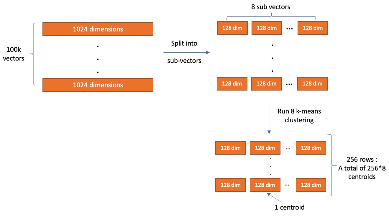
The main idea of PQ is to break up a vector into several sub-vectors and encode the sub-vectors independently with a fixed number of bits. The number of sub-vectors that the original vector is broken up into is controlled by a parameter, m, and the number of bits to encode each sub-vector with is controlled by a parameter, code_size. After encoding finishes, a vector is compressed into roughly m * code_size bits. So, assume we have a set of 100,000 1024-dimensional vectors. With m = 8 and code_size = 8, PQ breaks each vector into 8 128-dimensional sub-vectors and encode each sub-vector with 8 bits.

The values used for encoding are produced during a training step. During training, tables are created with 2code_size entries for each sub-vector partition. Next, k-Means clustering, with a k value of 2code_size, is run on the corresponding partition of sub-vectors from the training data. The centroids produced here are added as the entries to the partition’s table.

After all the tables are created, we encode a vector by replacing each sub-vector with the ID of the closest vector in the partition’s table. In the example where code_size = 8, we only need 8 bits to store an ID because there are 28 elements in the table. So, with dimension = 1024 and m = 8, the total size of one vector (assuming it uses a 32-bit floating point data type) is reduced from 4,096 bytes to roughly 8 bytes!

Product quantization encoding step

When we want to decode a vector, we can reconstruct an approximated version of it by using the stored IDs to retrieve the vectors from each partition’s table. The distance from the query vector to the reconstructed vector can then be computed and used in a nearest neighbor search. (It’s worth noting that, in practice, further optimization techniques like ADC are used to speed up this process for k-NN search).

Product quantization decoding step

Memory consumption

As we mentioned earlier, PQ will encode each vector into roughly m * code_size bits plus some overhead for each vector.

When combining it with IVF, we can estimate the index size as follows:

1.1 * ((((code_size/8) * m + overhead_per_vector) * num_vectors) + (4 * nlist * dimension) + (2 code_size * 4 * dimension) bytes

Using 1 billion vectors, dimension = 128, m = 8, code_size = 8, and nlist = 4096, we get an estimated total memory consumption of 70GB: 1.1 * ((((8 / 8) * 8 + 24) * 1,000,000,000) + (4 * 4096 * 128) + (2^8 * 4 * 128)) * 2 = 70 GB.

Running k-NN with OpenSearch

First make sure you have an OpenSearch cluster up and running. For instructions, refer to Cluster formation. For a more managed solution, you can use Amazon OpenSearch Service.

Before getting into the experiments, let’s go over how to run k-NN workloads in OpenSearch. First, we need to create an index. An index stores a set of documents in a way that they can be easily searched. For k-NN, the index’s mapping tells OpenSearch what algorithms to use and what parameters to use with them. We start by creating an index that uses HNSW as its search algorithm:

PUT my-hnsw-index
{
  "settings": {
    "index": {
      "knn": true,
      "number_of_shards": 10,
      "number_of_replicas" 1,
    }
  },
  "mappings": {
    "properties": {
      "my_vector": {
        "type": "knn_vector",
        "dimension": 4,
        "method": {
          "name": "hnsw",
          "space_type": "l2",
          "engine": "nmslib",
          "parameters": {
            "ef_construction": 128,
            "m": 24
          }
        }
      }
    }
  }
}

In the settings, we need to enable knn so that the index can be searched with the knn query type (more on this later). We also set the number of shards, and the number of replicas each shard will have. An index is made up of a collection of shards. Sharding is how OpenSearch distributes an index across multiple nodes in a cluster. For more information about shards, refer to Sizing Amazon OpenSearch Service domains.

In the mappings, we configure a field called my_vector of type knn_vector to store the vector data. We also pass nmslib as the engine to let OpenSearch know it should use nmslib’s implementation of HNSW. Additionally, we pass l2 as the space_type. The space_type determines the function used to compute the distance between two vectors. l2 refers to the Euclidean distance. OpenSearch also supports cosine similarity and the inner product distance functions.

After the index is created, we can ingest some fake data:

POST _bulk
{ "index": { "_index": "my-hnsw-index", "_id": "1" } }
{ "my_vector": [1.5, 2.5], "price": 12.2 }
{ "index": { "_index": "my-hnsw-index", "_id": "2" } }
{ "my_vector": [2.5, 3.5], "price": 7.1 }
{ "index": { "_index": "my-hnsw-index", "_id": "3" } }
{ "my_vector": [3.5, 4.5], "price": 12.9 }
{ "index": { "_index": "my-hnsw-index", "_id": "4" } }
{ "my_vector": [5.5, 6.5], "price": 1.2 }
{ "index": { "_index": "my-hnsw-index", "_id": "5" } }
{ "my_vector": [4.5, 5.5], "price": 3.7 }
{ "index": { "_index": "my-hnsw-index", "_id": "6" } }
{ "my_vector": [1.5, 5.5, 4.5, 6.4], "price": 10.3 }
{ "index": { "_index": "my-hnsw-index", "_id": "7" } }
{ "my_vector": [2.5, 3.5, 5.6, 6.7], "price": 5.5 }
{ "index": { "_index": "my-hnsw-index", "_id": "8" } }
{ "my_vector": [4.5, 5.5, 6.7, 3.7], "price": 4.4 }
{ "index": { "_index": "my-hnsw-index", "_id": "9" } }
{ "my_vector": [1.5, 5.5, 4.5, 6.4], "price": 8.9 }

After adding some documents to the index, we can search it:

GET my-hnsw-index/_search
{
  "size": 2,
  "query": {
    "knn": {
      "my_vector": {
        "vector": [2, 3, 5, 6],
        "k": 2
      }
    }
  }
}

Creating an index that uses IVF or PQ is a little bit different because these algorithms require training. Before creating the index, we need to create a model using the training API:

POST /_plugins/_knn/models/my_ivfpq_model/_train
{
  "training_index": "train-index",
  "training_field": "train-field",
  "dimension": 128,
  "description": "My model description",
  "method": {
      "name":"ivf",
      "engine":"faiss",
      "parameters":{
        "encoder":{
            "name":"pq",
            "parameters":{
                "code_size": 8,
                "m": 8
            }
        }
      }
  }
}

The training_index and training_field specify where the training data is stored. The only requirement for the training data index is that it has a knn_vector field that has the same dimension as you want your model to have. The method defines the algorithm that should be used for search.

After the training request is submitted, it will run in the background. To check if the training is complete, you can use the GET model API:

GET /_plugins/_knn/models/my_ivfpq_model/filter_path=model_id,state
{
  "model_id" : "my_ivfpq_model",
  "state" : "created"
}

After the model is created, you can create an index that uses this model:

PUT /my-hnsw-index
{
  "settings" : {
    "index.knn": true
    "number_of_shards" : 10,
    "number_of_replicas" : 1,
  },
  "mappings": {
    "properties": {
      "my_vector": {
        "type": "knn_vector",
        "model_id": "my_ivfpq_model"
      }
    }
  }
}

After the index is created, we can add documents to it and search it just like we did for HNSW.

Experiments

Let’s run a few experiments to see how these algorithms perform in practice and what tradeoffs are made. We look at an HNSW versus an IVF index using PQ. For these experiments, we’re interested in search accuracy, query latency, and memory consumption. Because these trade-offs are mainly observed at scale, we use the BIGANN dataset containing 1 billion vectors of 128 dimensions. The dataset also contains 10,000 queries of test data mapping a query to the ground truth closest 100 vectors based on the Euclidean distance.

Specifically, we compute the following search metrics:

  • Latency p99 (ms), Latency p90 (ms), Latency p50 (ms) – Query latency at various quantiles in milliseconds
  • recall@10 – The fraction of the top 10 ground truth neighbors found in the 10 results returned by the plugin
  • Native memory consumption (GB) – The amount of memory used by the plugin during querying

One thing to note is that the BIGANN dataset uses an unsigned integer as the data type. Because the knn_vector field doesn’t support unsigned integers, the data is automatically converted to floats.

To run the experiments, we complete the following steps:

  1. Ingest the dataset into the cluster using the OpenSearch Benchmarks framework (the code can be found on GitHub).
  2. When ingestion is complete, we use the warmup API to prepare the cluster for the search workload.
  3. We run the 10,000 test queries against the cluster 10 times and collect the aggregated results.

The queries return the document ID only, and not the vector, to improve performance (code for this can be found on GitHub).

Parameter selection

One tricky aspect of running experiments is selecting the parameters. There are too many different combinations of parameters to test them all. That being said, we decided to create three configurations for HNSW and IVFPQ:

  • Optimize for search latency and memory
  • Optimize for recall
  • Fall somewhere in the middle

For each optimization strategy, we chose two configurations.

For HNSW, we can tune the m, ef_construction, and ef_search parameters to achieve our desired trade-off:

  • m – Controls the maximum number of edges a node in a graph can have. Because each node has to store all of its edges, increasing this value will increase the memory footprint, but also increase the connectivity of the graph, which will improve recall.
  • ef_construction – Controls the size of the candidate queue for edges when adding a node to the graph. Increasing this value will increase the number of candidates to consider, which will increase the index latency. However, because more candidates will be considered, the quality of the graph will be better, leading to better recall during search.
  • ef_search – Similar to ef_construction, it controls the size of the candidate queue for graph traversal during search. Increasing this value will increase the search latency, but will also improve the recall.

In general, we chose configurations that gradually increased the parameters, as detailed in the following table.

Config ID Optimization Strategy m ef_construction ef_search
hnsw1 Optimize for memory and search latency 8 32 32
hnsw2 Optimize for memory and search latency 16 32 32
hnsw3 Balance between latency, memory, and recall 16 128 128
hnsw4 Balance between latency, memory, and recall 32 256 256
hnsw5 Optimize for recall 32 512 512
hnsw6 Optimize for recall 64 512 512

For IVF, we can tune two parameters:

  • nlist – Controls the granularity of the partitioning. The recommended value for this parameter is a function of the number of vectors in the index. One thing to keep in mind is that there are Faiss indexes that map to Lucene segments. There are several Lucene segments per shard and several shards per OpenSearch index. For our estimates, we assumed that there would be 100 segments per shard and 24 shards, so about 420,000 vectors per Faiss index. With this value, we estimated a good value to be 4096 and kept this constant for the experiments.
  • nprobes – Controls the number of nlist buckets we search. Higher values generally lead to improved recalls at the expense of increased search latencies.

For PQ, we can tune two parameters:

  • mControls the number of partitions to break the vector into. The larger this value is, the better the encoding will approximate the original, at the expense of raising memory consumption.
  • code_sizeControls the number of bits to encode a sub-vector with. The larger this value is, the better the encoding approximates the original, at the expense of raising memory consumption. The max value is 8, so we kept it constant at 8 for all experiments.

The following table summarizes our strategies.

Config ID Optimization Strategy nprobes m (num_sub_vectors)
ivfpq1 Optimize for memory and search latency 8 8
ivfpq2 Optimize for memory and search latency 16 8
ivfpq3 Balance between latency, memory, and recall 32 16
ivfpq4 Balance between latency, memory, and recall 64 32
ivfpq5 Optimize for recall 128 16
ivfpq6 Optimize for recall 128 32

Additionally, we need to figure out how much training data to use for IVFPQ. In general, Faiss recommends between 30,000 and 256,000 training vectors for components involving k-Means training. For our configurations, the maximum k for k-Means is 4096 from the nlist parameter. With this formula, the recommended training set size is between 122,880 and 1,048,576 vectors, so we settled on 1 million vectors. The training data comes from the index vector dataset.

Lastly, for the index configurations, we need to select the shard count. It is recommended to keep the shard size between 10–50 GBs for OpenSearch. Experimentally, we determined that for HNSW, a good number would be 64 shards and for IVFPQ, 42. Both index configurations were configured with one replica.

Cluster configuration

To run these experiments, we used Amazon OpenSearch Service using version 1.3 of OpenSearch to create the clusters. We decided to use the r5 instance family, which provides a good trade-off between memory size and cost.

The number of nodes will depend on the amount of memory that can be used for the algorithm per node and the total amount of memory required by the algorithm. Having more nodes and more memory will generally improve performance, but for these experiments, we want to minimize cost. The amount of memory available per node is computed as memory_available = (node_memory - jvm_size) * circuit_breaker_limit, with the following parameters:

  • node_memory – The total memory of the instance.
  • jvm_size – The OpenSearch JVM heap size. Set to 32 GB.
  • circuit_breaker_limit – The native memory usage threshold for the circuit breaker. Set to 0.5.

Because HNSW and IVFPQ have different memory requirements, we estimate how much memory is needed for each algorithm and determine the required number of nodes accordingly.

For HNSW, with m = 64, the total memory required using the formula from the previous sections is approximately 2,252 GB. Therefore, with r5.12xlarge (384 GB of memory), memory_available is 176 GB and the total number of nodes required is about 12, which we round up to 16 for stability purposes.

Because the IVFPQ algorithm requires less memory, we can use a smaller instance type, the r5.4xlarge instance, which has 128 GB of memory. Therefore, the memory_available for the algorithm is 48 GB. The estimated algorithm memory consumption where m = 64 is a total of 193 GB and the total number of nodes required is four, which we round up to six for stability purposes.

For both clusters, we use c5.2xlarge instance types as dedicated leader nodes. This will provide more stability for the cluster.

According to the AWS Pricing Calculator, for this particular use case, the cost per hour of the HNSW cluster is around $75 an hour, and the IVFPQ cluster costs around $11 an hour. This is important to remember when comparing the results.

Also, keep in mind that these benchmarks can be run using your custom infrastructure, using Amazon Elastic Compute Cloud (Amazon EC2), as long as the instance types and their memory size is equivalent.

Results

The following tables summarize the results from the experiments.

Test ID p50 Query latency (ms) p90 Query latency (ms) p99 Query latency (ms) Recall@10 Native memory consumption (GB)
hnsw1 9.1 11 16.9 0.84 1182
hnsw2 11 12.1 17.8 0.93 1305
hnsw3 23.1 27.1 32.2 0.99 1306
hnsw4 54.1 68.3 80.2 0.99 1555
hnsw5 83.4 100.6 114.7 0.99 1555
hnsw6 103.7 131.8 151.7 0.99 2055
Test ID p50 Query latency (ms) p90 Query latency (ms) p99 Query latency (ms) Recall@10 Native memory consumption (GB)
ivfpq1 74.9 100.5 106.4 0.17 68
ivfpq2 78.5 104.6 110.2 0.18 68
ivfpq3 87.8 107 122 0.39 83
ivfpq4 117.2 131.1 151.8 0.61 114
ivfpq5 128.3 174.1 195.7 0.40 83
ivfpq6 163 196.5 228.9 0.61 114

As you might expect, given how many more resources it uses, the HNSW cluster has lower query latencies and better recall. However, the IVFPQ indexes use significantly less memory.

For HNSW, increasing the parameters does in fact lead to better recall at the expense of latency. For IVFPQ, increasing m has the most significant impact on improving recall. Increasing nprobes improves the recall marginally, but at the expense of significant increases in latencies.

Conclusion

In this post, we covered different algorithms and techniques used to perform approximate k-NN search at scale (over 1 billion data points) within OpenSearch. As we saw in the previous benchmarks section, there isn’t one algorithm or approach that optimises for all the metrics at once. HNSW, IVF, and PQ each allow you to optimize for different metrics in your k-NN workload. When choosing the k-NN algorithm to use, first understand the requirements of your use case (How accurate does my approximate nearest neighbor search need to be? How fast should it be? What’s my budget?) and then tailor the algorithm configuration to meet them.

You can take a look at the benchmarking code base we used on GitHub. You can also get started with approximate k-NN search today following the instructions in Approximate k-NN search. If you’re looking for a managed solution for your OpenSearch cluster, check out Amazon OpenSearch Service.


About the Authors

Jack Mazanec is a software engineer working on OpenSearch plugins. His primary interests include machine learning and search engines. Outside of work, he enjoys skiing and watching sports.

Othmane Hamzaoui is a Data Scientist working at AWS. He is passionate about solving customer challenges using Machine Learning, with a focus on bridging the gap between research and business to achieve impactful outcomes. In his spare time, he enjoys running and discovering new coffee shops in the beautiful city of Paris.
Scaling Git’s garbage collection

Post Syndicated from Taylor Blau original https://github.blog/2022-09-13-scaling-gits-garbage-collection/

At GitHub, we store a lot of Git data: more than 18.6 petabytes of it, to be precise. That’s more than six times the size of the Library of Congress’s digital collections1. Most of that data comes from the contents of your repositories: your READMEs, source files, tests, licenses, and so on.

But some of that data is just junk: some bit of your repository that is no longer important. It could be a file that you force-pushed over, or the contents of a branch you deleted without merging. In general, this slice of repository data is anything that isn’t contained in at least one of your repository’s branches or tags. Normally, we don’t remove any unreachable data from repositories. But occasionally we do, usually to remove sensitive data, like passwords or SSH keys from your repository’s history.

The process for permanently removing unreachable objects from a repository’s history has a history of causing problems within GitHub, especially in busy repositories or ones with lots of objects. In this post, we’ll talk about what those problems were, why we had them, the tools we built to address them, and some interesting ways we’ve built on top of them. All of this work was contributed upstream to the open-source Git project. Let’s dive in.

Object reachability

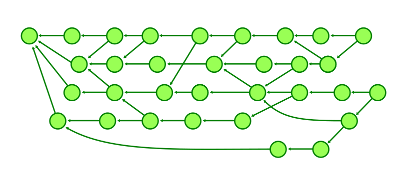
In this post, we’re going to talk a lot about “reachable” and “unreachable” objects. You may have heard these terms before, but perhaps only casually. Since we’re going to use them a lot, it will help to have more concrete definitions of the two. An object is reachable when there is at least one branch or tag along which you can reach the object in question. An object is “reached” by crawling through history—from commits to their parents, commits to their root trees, and trees to their sub-trees and blobs. An object is unreachable when no such branch or tag exists.

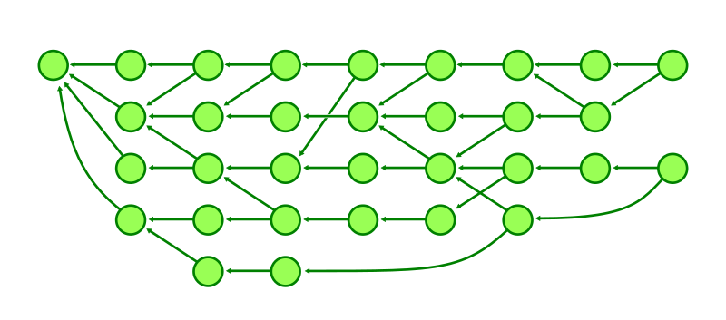
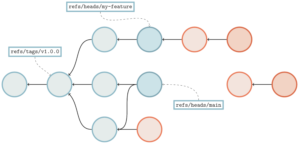
Sample object graph showing commits, with arrows connecting them to their parents. A few commits have boxes that are connected to them, which represent the tips of branches and tags.

Here, we’re looking at a sample object graph. For simplicity, I’m only showing commits (identified here as circles). Arrows point from commits to their parent(s). A few commits have boxes that are connected to them, which represent the tips of branches and tags.

The parts of the graph that are colored blue are reachable, and the red parts are considered unreachable. You’ll find that if you start at any branch or tag, and follow its arrows, that all commits along that path are considered reachable. Note that unreachable commits which have reachable ones as parents (in our diagram above, anytime an arrow points from a red commit to a blue one) are still considered unreachable, since they are not contained within any branch or tag.

Unreachable objects can also appear in clusters that are totally disconnected from the main object graph, as indicated by the two lone red commits towards the right-hand side of the image.

Pruning unreachable objects

Normally, unreachable objects stick around in your repository until they are either automatically or manually cleaned up. If you’ve ever seen the message, “Auto packing the repository for optimum performance,” in your terminal, Git is doing this for you in the background. You can also trigger garbage collection manually by running:

$ git gc --prune=<date>

That tells Git to trigger a garbage collection and remove unreachable objects. But observant readers might notice the optional <date> parameter to the --prune flag. What is that? The short answer is that Git allows you to restrict which objects get permanently deleted based on the last time they were written. But to fully explain, we first need to talk a little bit about a race condition that can occur when removing objects from a Git repository.

Object deletion raciness

Normally, deleting an unreachable object from a Git repository should not be a notable event. Since the object is unreachable, it’s not part of any branch or tag, and so deleting it doesn’t change the repository’s reachable state. In other words, removing an unreachable object from a repository should be as simple as:

  1. Repacking the repository to remove any copies of the object in question (and recomputing any deltas that are based on that object).
  2. Removing any loose copies of the object that happen to exist.
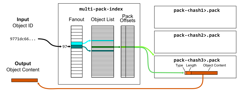
  3. Updating any additional indexes (like the multi-pack index, or commit-graph) that depend on the (now stale) packs that were removed.

The racy behavior occurs when a repository receives one or more pushes during this process. The main culprit is that the server advertises its objects at a different point in time from processing the objects that the client sent based on that advertisement.

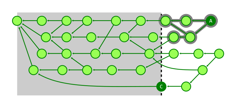
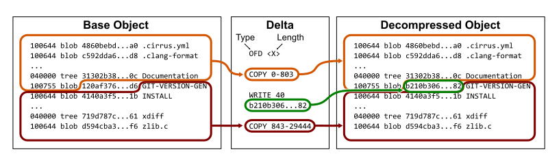
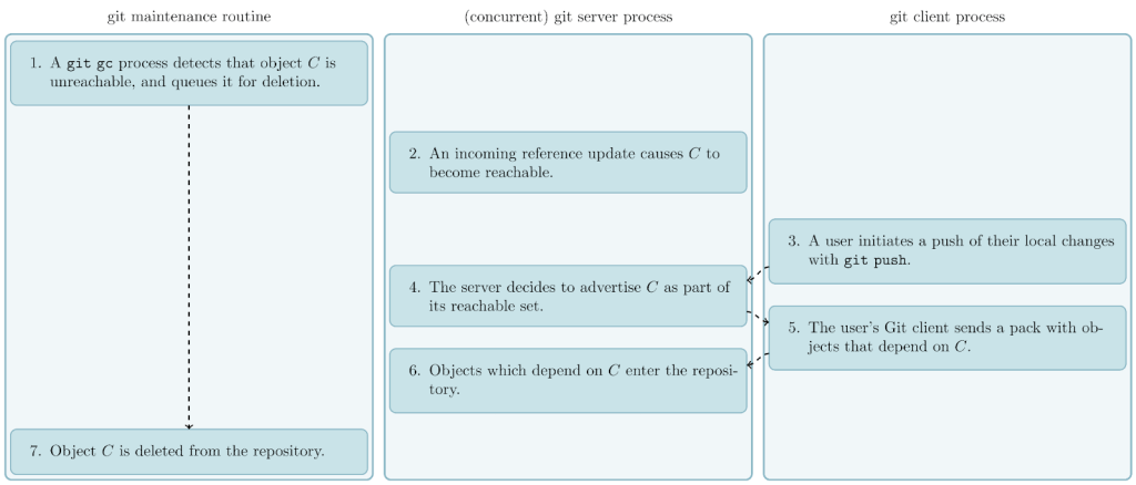
Consider what happens if Git decides (as part of running a git gc operation) that it wants to delete some unreachable object C. If C becomes reachable by some background reference update (e.g., an incoming push that creates a new branch pointing at C), it will then be advertised to any incoming pushes. If one of these pushes happens before C is actually removed, then the repository can end up in a corrupt state. Since the pusher will assume C is reachable (since it was part of the object advertisement), it is allowed to include objects that either reference or depend on C, without sending C itself. If C is then deleted while other reachable parts of the repository depend on it, then the repository will be left in a corrupt state.

Suppose the server receives that push before proceeding to delete C. Then, any objects from the incoming push that are related to it would be immediately corrupt. Reachable parts of the repository that reference C are no longer closed2 over reachability since C is missing. And any objects that are stored as a delta against C can no longer be inflated for the same reason.

Figure demonstrating that one side (responsible for garbage collecting the repository) decides that a certain object is unreachable, while another side makes that object reachable and accepts an incoming push based on that object—before the original side ultimately deletes that (now-reachable) object—leaving the repository in a corrupt state.

In case that was confusing, the above figure should help clear things up. The general idea is that one side (responsible for garbage collecting the repository) decides that a certain object is unreachable, while another side makes that object reachable and accepts an incoming push based on that object—before the original side ultimately deletes that (now-reachable) object—leaving the repository in a corrupt state.

Mitigating object deletion raciness

Git does not completely prevent this race from happening. Instead, it works around the race by gradually expiring unreachable objects based on the last time they were written. This explains the mysterious --prune=<date> option from a few sections ago: when garbage collecting a repository, only unreachable objects which haven’t been written since <date> are removed. Anything else (that is, the set of objects that have been written at least once since <date>) are left around.

The idea is that objects which have been written recently are more likely to become reachable again in the future, and would thus be more likely to be susceptible to the kind of race we talked about above if they were to be pruned. Objects which haven’t been written recently, on the other hand, are proportionally less likely to become reachable again, and so they are safe (or, at least, safer) to remove.

This idea isn’t foolproof, and it is certainly possible to run into the race we talked about earlier. We’ll discuss one such scenario towards the end of this post (along with the way we worked around it). But in practice, this strategy is simple and effective, preventing most instances of potential repository corruption.

Storing loose unreachable objects

But one question remains: how does Git keep track of the age of unreachable objects which haven’t yet aged out of the repository?

The answer, though simple, is at the heart of the problem we’re trying to solve here. Unreachable objects which have been written too recently to be removed from the repository are stored as loose objects, the individual object files stored in .git/objects. Storing these unreachable objects individually means that we can rely on their stat() modification time (hereafter, mtime) to tell us how recently they were written.

But this leads to an unfortunate problem: if a repository has many unreachable objects, and a large number of them were written recently, they must all be stored individually as loose objects. This is undesirable for a number of reasons:

  • Pairs of unreachable objects that share a vast majority of their contents must be stored separately, and can’t benefit from the kind of deduplication offered by packfiles. This can cause your repository to take up much more space than it otherwise would.
  • Having too many files (especially too many in a single directory) can lead to performance problems, including exhausting your system’s available inodes in the extreme case, leaving you unable to create new files, even if there may be space available for them.
  • Any Git operation which has to scan through all loose objects (for example, git repack -d, which creates a new pack containing just your repository’s unpacked objects) will slow down as there are more files to process.

It’s tempting to want to store all of a repository’s unreachable objects into a single pack. But there’s a problem there, too. Since all of the objects in a single pack share the same mtime (the mtime of the *.pack file itself), rewriting any single unreachable object has the effect of updating the mtimes of all of a repository’s unreachable objects. This is because Git optimizes out object writes for packed objects by simply updating the mtime of any pack(s) which contain that object. This makes it nearly impossible to expire any objects out of the repository permanently.

Cruft packs

To solve this problem, we turned to a long-discussed idea on the Git mailing list: cruft packs. The idea is simple: store an auxiliary list of mtime data alongside a pack containing just unreachable objects. To garbage collect a repository, Git places the unreachable objects in a pack. That pack is designated as a “cruft pack” because Git also writes the mtime data corresponding to each object in a separate file alongside that pack. This makes it possible to update the mtime of a single unreachable object without changing the mtimes of any other unreachable object.

To give you a sense of what this looks like in practice, here’s a small example:

a pack of Git objects (represented by rectangles of different colors)

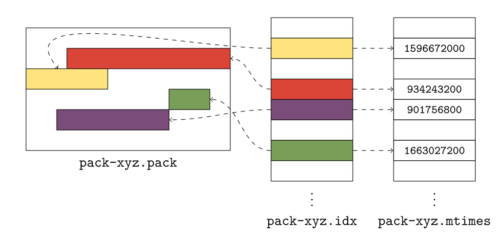
The above figure shows a pack of Git objects (represented by rectangles of different colors), its pack index, and the new .mtimes file. Together, these three files make up what Git calls a “cruft pack,” and it’s what allows Git to store unreachable objects together, without needing a single file for each object.

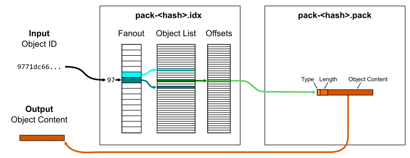
So, how do they work? Git uses the cruft pack to store a collection of object mtimes together in an array stored in the *.mtimes file. In order to discover the mtime for an individual object in a pack, Git first does a binary search on the pack’s index to discover that object’s lexicographic index. Git can then use that offset to read a 4-byte, unsigned integer in the .mtimes file. The .mtimes file contains a table of integers (one for each object in the associated *.pack file), each representing an epoch timestamp containing that object’s mtime. In other words, the *.mtimes file has a table of numbers, where each number represents an individual object’s mtime, encoded as a number of seconds since the Unix epoch.

Crucially, this makes it possible to store all of a repository’s unreachable objects together in a single pack, without having to store them as individual loose objects, bypassing all of the drawbacks we discussed in the last section. Moreover, it allows Git to update the mtime of a single unreachable object, without inadvertently triggering the same update across all unreachable objects.

Since Git doesn’t portably support updating a file in place, updating an object’s mtime (a process which Git calls “freshening”) takes place by writing a separate copy of that object out as a loose file. Of course, if we had to freshen all objects in a cruft pack, we would end up in a situation no better than before. But such updates tend to be unlikely in practice, and so writing individual copies of a small handful of unreachable objects ends up being a reasonable trade off most of the time.

Generating cruft packs

Now that we have introduced the concept of cruft packs, the question remains: how does Git generate them?

Despite being called git gc (short for “garbage collection”), running git gc does not always result in deleting unreachable objects. If you run git gc --prune=never, then Git will repack all reachable objects and move all unreachable objects to the cruft pack. If, however, you run git gc --prune=1.day.ago, then Git will repack all reachable objects, delete any unreachable objects that are older than one day, and repack the remaining unreachable objects into the cruft pack.

This is because of Git’s treatment of unreachable parts of the repository. While Git only relies on having a reachability closure over reachable objects, Git’s garbage collection routine tries to leave unreachable parts of the repository intact to the extent possible. That means if Git encounters some unreachable cluster of objects in your repository, it will either expire all or none of those objects, but never some subset of them.

We’ll discuss how cruft packs are generated with and without object expiration in the two sections below.

Cruft packs without object expiration

When generating a cruft pack with an object expiration of --date=never, our only goal is to collect all unreachable objects together into a single cruft pack. Broadly speaking, this occurs in three steps:

  1. Starting at all of the branches and tags, generate a pack containing only reachable objects.
  2. Looking at all other existing packs, enumerate the list of objects which don’t appear in the new pack of reachable objects. Create a new pack containing just these objects, which are unreachable.
  3. Delete the existing packs.

If any of that was confusing, don’t worry: we’ll break it down here step by step. The first step to collecting a repository’s unreachable objects is to figure out the parts of it that are reachable. If you’ve ever run git repack -A, this is exactly how that command works. Git starts a reachability traversal beginning at each of the branches and tags in your repository. Then it traverses back through history by walking from commits to their parents, trees to their sub-trees, and so on, marking every object that it sees along the way as reachable.

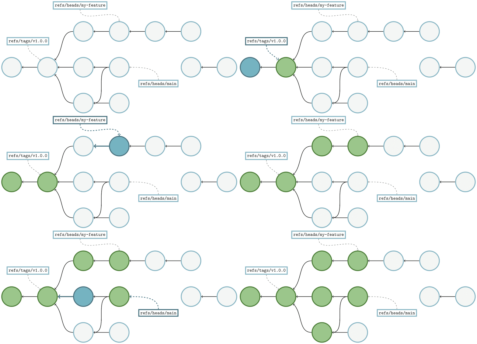
Demonstration of how Git walks through a commit graph, from commit to parent

Here, we’re showing the same commit graph from earlier in the post. Git’s goal at this point is simply to mark every reachable object that it sees, and it’s those objects that will become the contents of a new pack containing just reachable objects. Git starts by examining each reference, and walking from a commit to its parents until it either finds a commit with no parents (indicating the beginning of history), or a commit that it has already marked as reachable.

In the above, the commit being walked is highlighted in dark blue, and any commits marked as reachable are marked in green. At each step, the commit currently being visited gets marked as reachable, and its parent(s) are visited in the next step. By repeating this process among all branches and tags, Git will mark all reachable objects in the repository.

We can then use this set of objects to produce a new pack containing all reachable objects in a repository. Next, Git needs to discover the set of objects that it didn’t mark in the previous stage. A reasonable first approach might be to store the IDs of all of a repository’s objects in a set, and then remove them one by one as we mark objects reachable along our walk.

But this approach tends to be impractical, since each object will require a minimum of 20 bytes of memory in order to insert into this set. At the time of writing, the linux.git repository contains nearly nine million objects, which would require nearly 180 MB of memory just to write out all of their object IDs.

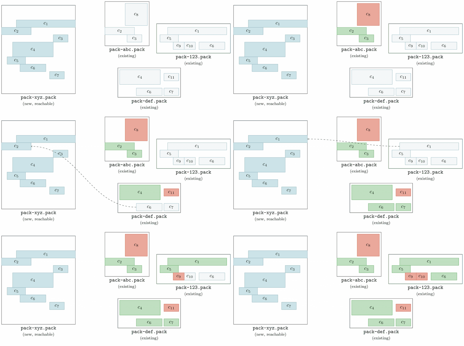
Instead, Git looks through all of the objects in all of the existing packs, checking whether or not each is contained in the new pack of reachable objects. Any object found in an existing pack which doesn’t appear in the reachable pack is automatically included in the cruft pack.

Animation demonstrating how  Git looks through all of the objects in all of the existing packs, checking whether or not each is contained in the new pack of reachable objects.

Here, we’re going one by one among all of the pre-existing packs (here, labeled as pack-abc.pack, pack-def.pack, and pack-123.pack) and inspecting their objects one at a time. We first start with object c8, looking through the reachable pack (denoted as pack-xyz.pack) to see if any of its objects match c8. Since none do, c8 is marked unreachable (which we represent by filling the object with a red background).

This process is repeated for each object in each existing pack. Once this process is complete, all objects that existed in the repository before starting a garbage collection are marked either green, or red (indicating that they are either reachable, or unreachable, respectively).

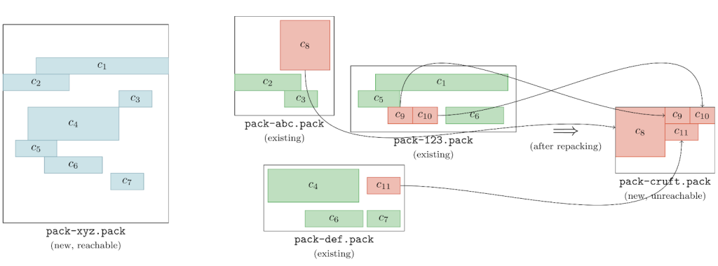
Git can then use the set of unreachable objects to generate a new pack, like below:

A set of labeled Git packs

This pack (on the far right of the above image, denoted pack-cruft.pack) contains exactly the set of unreachable objects present in the repository at the beginning of garbage collection. By keeping track of each unreachable object’s mtime while marking existing objects, Git has enough data to write out a *.mtimes file in addition to the new pack, leaving us with a cruft pack containing just the repository’s unreachable objects.

Here, we’re eliding some technical details about keeping track of each object’s mtime along the way, for brevity and simplicity. The routine is straightforward, though: each time we discover an object, we mark its mtime based on how we discovered the object.

  • If an object is found in a packfile, it inherits its mtime from the packfile itself.
  • If an object is found as a loose object, its mtime comes from the loose object file.
  • And if an object is found in an existing cruft pack, its mtime comes from reading the cruft pack’s *.mtimes file at the appropriate index.

If an object is seen more than once (e.g., an unreachable object stored in a cruft pack was freshened, resulting in another loose copy of the object), the mtime which is ultimately recorded in the new cruft pack is the most recent mtime of all of the above.

Cruft packs with object expiration

Generating cruft packs where some objects are going to expire out of the repository follows a similar, but slightly trickier approach than in the non-expiring case.

Doing a garbage collection with a fixed expiration is known as “pruning.” This essentially boils down to asking Git to pack the contents of a repository into two packfiles: one containing reachable objects, and another containing any unreachable objects. But, it also means that for some fixed expiration date, any unreachable objects which have an mtime older than the expiration date are removed from the repository entirely.

The difficulty in this case stems from a fact briefly mentioned earlier in this post, which is that Git attempts to prevent connected clusters of unreachable objects from leaving the repository if some, but not all, of their objects have aged out.

To make things clearer, here’s an example. Suppose that a repository has a handful of blob objects, all connected to some tree object, and all of these objects are unreachable. Assuming that they’re all old enough, then they will all expire together: no big deal. But what if the tree isn’t old enough to be expired? In this case, even though the blobs connected to it could be expired on their own, Git will keep them around since they’re connected to a tree with a sufficiently recent mtime. Git does this to preserve the repository’s reachability closure in case that tree were to become reachable again (in which case, having the tree and its blobs becomes important).

To ensure that Git preserves any unreachable objects which are reachable from recent objects Git handles this case of cruft pack generation slightly differently. At a high level, it:

  1. Generates a candidate list of cruft objects, using the same process as outlined in the previous section.
  2. Then, to determine the actual list of cruft objects to keep around, it performs a reachability traversal using all of the candidate cruft objects, adding any object it sees along the way to the cruft pack.

To make things a little clearer, here’s an example:

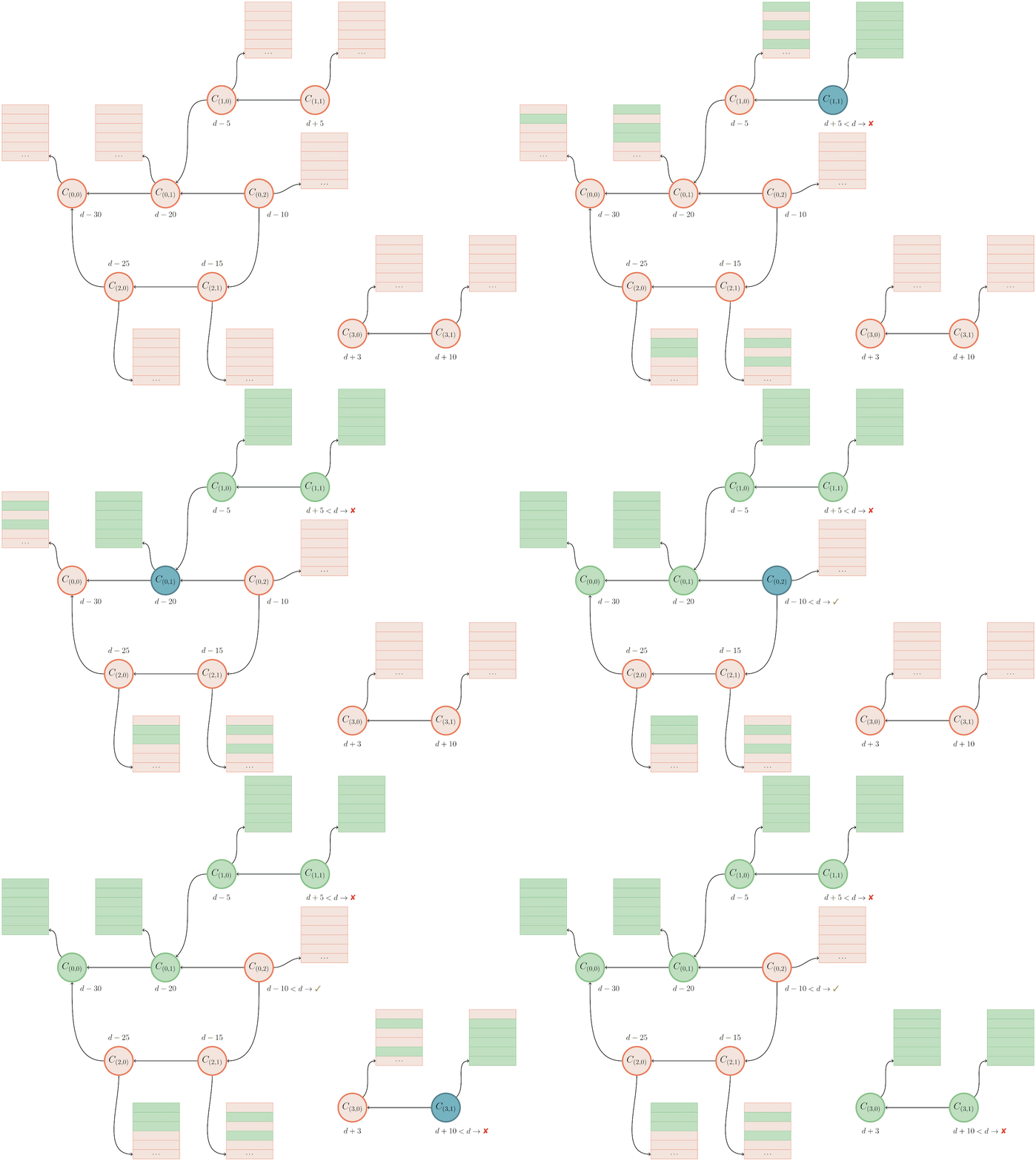
Animation of Git performing  a reachability traversal

After determining the set of unreachable objects (represented above as colored red) Git does a reachability traversal from each entry point into the graph of unreachable objects. Above, commits are represented by circles, trees by rectangles, and tree entries as rows within the larger rectangles. The mtimes are written below each commit.

For now, let’s assume our expiration date is d, so any object whose mtime is greater than d must stay (despite being unreachable), and anything older than d can be pruned. Git traverses through each entry and asks, “Is this object old enough to be pruned?” When the answer is “yes” Git leaves the object alone and moves on to the next entry point. When the answer is “no,” however, (ie., Git is looking at an unreachable object whose mtime is too recent to prune), Git marks that object as “rescued” (indicated by turning it green) and then continues its traversal, marking any reachable objects as rescued.

Objects that are rescued during this pass are written to the cruft pack, preserving their existence in the repository, leaving them to either continue to age, or have their mtimes updated before the next garbage collection.

Let’s take a closer look at the example above. Git starts by looking at object C(1,1), and notice that its mtime is d+5, meaning that (since it happens after our expiration time, d) it is too new to expire. That causes Git to start a reachability traversal beginning at C(1,1), rescuing every object it encounters along the way. Since many objects are shared between multiple commits, rescuing an object from a more recent part of the graph often ends up marking older objects as rescued, too.

After finishing the rescuing pass focused on C(1,1), Git moves on to look at C(0,2). But this commit’s mtime is d-10, which is before our expiration cutoff of d, meaning that it is safe to remove. Git can skip looking at any objects reachable from this commit, since none of them will be rescued.

Finally, Git looks at another connected cluster of the unreachable object graph, beginning at C(3,1). Since this object has an mtime of d+10, it is too new to expire, so Git performs another reachability traversal, rescuing it and any objects reachable from it.

Notice that in the final graph state that the main cluster of commits (the one beginning with C(0,2)) is only partially rescued. In fact, only the objects necessary to retain a reachability closure over the rescued objects among that cluster are saved from being pruned. So even though, for example, commit C(2,1) has only part of its tree entries rescued, that is OK since C(2,1) itself will be pruned (hence any non-rescued tree entries connected to it are unimportant and will also be pruned).

Putting it all together

Now that Git can generate a cruft pack and perform garbage collection on a repository with or without pruning objects, it was time to put all of the pieces together and submit the patches to the open-source Git project.

Other Git sub-commands, like repack, and gc needed to learn about cruft packs, and gain command-line flags and configuration knobs in order to opt-in to the new behavior. With all of the pieces in place, you can now trigger a garbage collection by running either:

$ git gc --prune=1.day.ago --cruft

or

$ git repack -d --cruft --cruft-expiration=1.day.ago

to repack your repository into a reachable pack, and a cruft pack containing unreachable objects whose mtimes are within the past day. More details on the new command-line options and configuration can be found here, here, here, and here.

GitHub submitted the entirety of the patches that comprise cruft packs to the open-source Git project, and the results were released in v2.37.0. That means that you can use the same tools as what we run at GitHub on your own laptop, to run garbage collection on your own repositories.

For those curious about the details, you can read the complete thread on the mailing list archive here.

Cruft packs at GitHub

After a lengthy process of testing to ensure that using cruft packs was safe to carry out across all repositories on GitHub, we deployed and enabled the feature across all repositories. We kept a close eye on repositories with large numbers of unreachable objects, since the process of breaking any deltas between reachable and unreachable objects (since the two are now stored in separate packs, and object deltas cannot cross pack boundaries) can cause the initial cruft pack generation to take a long time. A small handful of repositories with many unreachable objects needed more time to generate their very first cruft pack. In those instances, we generated their cruft packs outside of our normal repository maintenance jobs to avoid triggering any timeouts.

Now, every repository on GitHub and in GitHub Enterprise (in version 3.3 and newer) uses cruft packs to store their unreachable objects. This has made garbage collecting repositories (especially busy ones with many unreachable objects) tractable where it often required significant human intervention before. Before cruft packs, many repositories which required clean up were simply out of our reach because of the possibility of creating an explosion of loose objects which could derail performance for all repositories stored on a fileserver. Now, garbage collecting a repository is a simple task, no matter its size or scale.

During our testing, we ran garbage collection on a handful of repositories, and got some exciting results. For repositories that regularly force-push a single commit to their main branch (leaving a majority of their objects unreachable), their on-disk size dropped significantly. The most extreme example we found during testing caused a repository which used to take 186 gigabytes to store shrink to only take 2 gigabytes of space.

On github/github, GitHub’s main codebase, we were able to shrink the repository from around 57 gigabytes to 27 gigabytes. Even though these savings are more modest, the real payoff is in the objects we no longer have to store. Before garbage collecting, each replica of this repository had nearly 60 million objects, including years of test-merges, force-pushes, and all kinds of sources of unreachable objects. Each of these objects contributed to the I/O cost of repacking this repository. After garbage collecting, only 11.8 million objects remained. Since each object in a repository requires around 150 bytes of memory during repacking, we save around 7 gigabytes of RAM during each maintenance routine.

Limbo repositories

Even though we can easily garbage collect a repository of any size, we still have to navigate the inherent raciness that we described at the beginning of this post.

At GitHub, our approach has been to make this situation easy to recover from automatically instead of preventing it entirely (which would require significant surgery to much of Git’s code). To do this, our approach is to create a “limbo” repository whenever a pruning garbage collection is done. Any objects which get expired from the main repository are stored in a separate pack in the limbo repository. Then, the process to garbage collect a repository looks something like:

  1. Generate a cruft pack of recent unreachable objects in the main repository.
  2. Generate a second cruft pack of expired unreachable objects, stored outside of the main repository, in the “limbo” repository.
  3. After garbage collection has completed, run a git fsck in the main repository to detect any object corruption.
  4. If any objects are missing, recover them by copying them over from the limbo repository.

The process for generating a cruft pack of expired unreachable objects boils down to creating another cruft pack (using exactly the same process we described earlier in this post), with two caveats:

  • The expiration cutoff is set to “never” since we want to keep around any objects which we did expire in the previous step.
  • The original cruft pack is treated as a pack containing reachable objects since we want to ignore any unreachable objects which were too recent to expire (and, thus, are stored in the cruft pack in the main repository).

We have used this idea at GitHub with great success, and now treat garbage collection as a hands-off process from start to finish. The patches to implement this approach are available as a preliminary RFC on the Git mailing list here.

Thank you

This work would not have been possible without generous review and collaboration from engineers from within and outside of GitHub. The Git Systems team at GitHub were great to work with while we developed and deployed cruft packs. Special thanks to Torsten Walter, and Michael Haggerty, who played substantial roles in developing limbo repositories.

Outside of GitHub, this work would not have been possible without careful review from the open-source Git community, especially Derrick Stolee, Jeff King, Jonathan Tan, Jonathan Nieder, and Junio C Hamano. In particular, Jeff King contributed significantly to the original development of many of the ideas discussed above.

Notes


  1. It’s true. According to the Library of Congress themselves, their digital collection amounts to more than 3 petabytes in size [source]. The 18.6 petabytes we store at GitHub actually overcounts by a factor of five, since we store a handful of copies of each repository. In reality, it’s hard to provide an exact number, since data is de-duplicated within a fork network, and is stored compressed on disk. Either way you slice it, it’s a lot of data: you get the point. 
  2. Meaning that for any reachable object part of some repository, any objects reachable from it are also contained in that repository. 

Contributing to open source at GitHub

Post Syndicated from Ariel Deitcher original https://github.blog/2022-09-06-contributing-to-open-source-at-github/

Ariel Deitcher (@mntlty) is a Senior Software Engineer at GitHub, working on Pull Requests and Merge Queue (beta). In this post, he shares the challenges he encountered finding his path to contributing to open source, what it was like contributing to open source at GitHub, and some of the lessons he learned.

Getting started with open source can be overwhelming

As a computer science graduate in 2011 and searching for my first tech job, I read that contributing to an open source project could help. It was a great way to build skills, make industry connections, and gain practical experience with a real-world problem. Perfect, I thought, I’ll just pick an open source project on this new website called GitHub, and, well, actually I wasn’t sure how to do that. Finding that “Goldilocks” project (where the size, language(s), domain, and community felt just right) was a lot harder than I thought, and I didn’t feel self-confident enough to make much progress. Overwhelmed, I decided the timing wasn’t right but resolved to try again someday.

It bugged me that the contribution graph on my GitHub profile remained stubbornly empty, as all the code I had committed lived in private repositories. That changed in 2016 when contributions to private repositories could be shown on my profile, but my contributions to open source had not. Between my family, work, life, and the explosive growth in projects to choose from, making that first contribution to open source felt more daunting than ever.

The opportunity to contribute to open source at GitHub

Fast forward to 2021. I read Working in Public: The Making and Maintenance of Open Source Software by Nadia Eghbal while interviewing at GitHub. I was especially captivated by the Stadium model of open source projects, where a small number of maintainers and occasional contributors are vastly outnumbered by a project’s users. This aligned with my mental model of open source projects, where a few performers on a digital stage would conjure feats of coding wizardry. I could only imagine how vulnerable working in public could be, and hoped it would feel less intimidating working at GitHub.

I joined the GitHub team building Merge Queue (beta), a feature which helps users coordinate their merges to a protected branch, ensures that changes are up to date, and that all required checks pass before automatically merging a pull request. Early on, I shared my long-held goal of contributing code to an open source project with my manager, and discussed the GitHub CLI, an open source tool written in Go which lets users interact with GitHub from the command line, as a possible candidate.

While building Merge Queue, our team carefully integrated it with GitHub’s many APIs and tools, checking each one for compatibility and correctness. Testing different scenarios of merging a pull request with the GitHub CLI, I saw that once a Merge Queue was required, running the CLI command gh pr merge would fail in most cases. The Merge Queue was correctly preventing direct merges to its protected branch, and so I began scoping out what changes the CLI might need to support Merge Queue.

As I didn’t have write access to the CLI repository, I forked it, started a new Codespace, and spent some time getting familiar with the CLI’s contributing guidelines and code. Wanting to minimize my changes, I targeted a few places in the merge command to modify. When I was ready, I pushed a commit to my fork and opened a pull request to share with the CLI maintainers. I expected that I would provide support but defer to them for the final implementation.

In reviewing my pull request with the CLI maintainers, it quickly became clear that my changes were hard to reason about. The merge command had accumulated sufficient technical debt that adding more complexity to it was risky. The team asked if I could refactor the merge command in an initial pull request and follow up with a subsequent pull request for the Merge Queue changes after the first was merged. What I had thought would be a rough guide of changes for the CLI maintainers was, in fact, the opportunity I had been looking for to contribute to open source at GitHub. I confirmed that my manager was onboard with this increased commitment, and was ready to get started.

Refactoring the merge command and adding Merge Queue support

I set out to refactor the merge command with a focus on simplicity, readability, and returning early over deeply nested conditionals. The existing test coverage gave me a confidence boost as I began stepping through the code, copying each section into a separate file for later reference, and wrote comments which I felt captured the intent of the removed section. I then grouped related Git and API operations, consolidated common code into appropriately named functions and variables, trimmed unreachable code paths, created a MergeContext struct to encapsulate state, and leaned into Go’s explicit error returns – all of which gave the code a more linear and consistent structure.

As an example, the mergeRun function, which is the heart of the merge command, went from over 220 lines to just 30:

func mergeRun(opts *MergeOptions) error {
    ctx, err := NewMergeContext(opts)
    if err != nil {
        return err
    }

    // no further action is possible when disabling auto merge
    if opts.AutoMergeDisable {
        return ctx.disableAutoMerge()
    }

    ctx.warnIfDiverged()

    if err := ctx.canMerge(); err != nil {
        return err
    }

    if err := ctx.merge(); err != nil {
        return err
    }

    if err := ctx.deleteLocalBranch(); err != nil {
        return err
    }

    if err := ctx.deleteRemoteBranch(); err != nil {
        return err
    }

    return nil
}

When I was finished, I opened a pull request from my fork to the CLI repository, and was blown away by how supportive the code review process was. After a few rounds of feedback, my code was merged and ready to ship in the next release. I was an open source contributor at GitHub!

Returning to my fork, my original Merge Queue changes were now completely out of date. In fact, much of the code I had on my branch no longer existed on the CLI’s trunk branch. Fortunately, I was now intimately familiar with the merge command and was able to make the Merge Queue changes and tests in a subsequent pull request quickly and with confidence.

Lessons learned

Looking back, I learned that searching for the right open source project on my own, trying to create time outside of work, and context switching from my existing projects were obstacles I could not overcome. Instead, the key for me was to find an open source project that was important to what I was already working on, and that I was accountable for. If this sounds familiar, consider asking your manager if you can devote some time to work on an issue in an open source project that you or your team rely on. It’s much easier to get started with an open source project you know and can align with work you’re already committed to. I recognize how fortunate I was to be in the right place at the right time, and with the right support from my manager, but it wasn’t easy.

Many people I know struggle with impostor syndrome, and working in public made me even more aware of mine. I am learning to accept that even though my commits aren’t perfect, and that I’m afraid of being judged for creating bugs like this regression, which will be discoverable forever, I should still contribute. Despite these challenges, I enjoy picking up new issues in the CLI labeled “help wanted (contributions welcome)” whenever I can, and hope you will too!

AWS Week in Review – September 5, 2022

Post Syndicated from Danilo Poccia original https://aws.amazon.com/blogs/aws/aws-week-in-review-september-5-2022/

This post is part of our Week in Review series. Check back each week for a quick roundup of interesting news and announcements from AWS!

As a new week begins, let’s quickly look back at the most significant AWS news from the previous seven days.

Last Week’s Launches
Here are the launches that got my attention last week:

AWS announces open-sourced credentials-fetcher to simplify Microsoft AD access from Linux containers. You can find more in the What’s New post.

AWS Step Functions now has 14 new intrinsic functions that help you process data more efficiently and make it easier to perform data processing tasks such as array manipulation, JSON object manipulation, and math functions within your workflows without having to invoke downstream services or add Task states.

AWS SAM CLI esbuild support is now generally available. You can now use esbuild in the SAM CLI build workflow for your JavaScript applications.

Amazon QuickSight launches a new user interface for dataset management that replaces the existing popup dialog modal with a full-page experience, providing a clearer breakdown of dataset management categories.

AWS GameKit adds Unity support. With this release for Unity, you can integrate cloud-based game features into Win64, MacOS, Android, or iOS games from both the Unreal and Unity engines with just a few clicks.

AWS and VMware announce VMware Cloud on AWS integration with Amazon FSx for NetApp ONTAP. Read more in Veliswa‘s blog post.

The AWS Region in the United Arab Emirates (UAE) is now open. More info in Marcia‘s blog post.

View of Abu Dhabi in the United Arab Emirates

For a full list of AWS announcements, be sure to keep an eye on the What’s New at AWS page.

Other AWS News
A few more blog posts you might have missed:

Easy analytics and cost-optimization with Amazon Redshift Serverless – Four different use cases of Redshift Serverless are discussed in this post.

Building cost-effective AWS Step Functions workflows – In this blog post, Ben explains the difference between Standard and Express Workflows, including costs, migrating from Standard to Express, and some interesting ways of using both together.

How to subscribe to the new Security Hub Announcements topic for Amazon SNS – You can now receive updates about new Security Hub services and features, newly supported standards and controls, and other Security Hub changes.

Deploying AWS Lambda functions using AWS Controllers for Kubernetes (ACK) – With the ACK service controller for AWS Lambda, you can provision and manage Lambda functions with kubectl and custom resources.

For AWS open-source news and updates, here’s the latest newsletter curated by Ricardo to bring you the most recent updates on open-source projects, posts, events, and more.

Upcoming AWS Events
Depending on where you are on this planet, there are many opportunities to meet and learn:

AWS Summits – Come together to connect, collaborate, and learn about AWS. Registration is open for the following in-person AWS Summits: Ottawa (September 8), New Delhi (September 9), Mexico City (September 21–22), Bogotá (October 4), and Singapore (October 6).

AWS Community DaysAWS Community Day events are community-led conferences to share and learn with one another. In September, the AWS community in the US will run events in the Bay Area, California (September 9) and Arlington, Virginia (September 30). In Europe, Community Day events will be held in October. Join us in Amersfoort, Netherlands (October 3), Warsaw, Poland (October 14), and Dresden, Germany (October 19).

That’s all from me for this week. Come back next Monday for another Week in Review!

Danilo

Git’s database internals V: scalability

Post Syndicated from Derrick Stolee original https://github.blog/2022-09-02-gits-database-internals-v-scalability/

This week, we are exploring Git’s internals with the following concept in mind:

Git is the distributed database at the core of your engineering system.

When the database at the core of an application approaches scale limits of a single database node, a common strategy is to shard the database. By splitting the database into multiple components, we can scale beyond the limits of a single node.

For Git, large repositories can have a similar feeling. While there exist some extremely large monorepos operating with success, they require careful attention and advanced features. For some, that effort is better spent sharding the repository. Just like sharding an application database, there are many ways to split a Git repository, with various trade-offs.

When sharding an application database, there are a number of factors to consider.

Some application databases include automatic horizontal sharding based on a shard key, which is usually a string literal that can be sorted lexicographically so related values appear in the same shard due to a common prefix in the shard key. There is no immediate way to shard Git’s object store in this way. The object IDs are hashes of the object contents and have essentially random prefixes.

Instead, we think of sharding strategies that split the repository by other structures, including logical components, paths in the worktree, and time periods in the commit history.

Component sharding: multi-repo

One way to shard an application database is to split out entire tables that can be operated independently and managed by independent services. The Git equivalent is to split a repository in to multiple smaller repositories with no concrete links between them. This creates a multi-repo sharding strategy.

The common approach to this strategy is to extract functionality out of a monolith into a microservice, but that microservice exists in its own Git repository that is not linked at all to the monolith’s repository. This effort might remove code from the monolith across multiple path prefixes due to the monolith’s architecture.

Multi-repo sharding strategy that extracts functionality out of a monolith into a microservice that exists in its own Git repository.

Using this strategy works best if each microservice is paired with a team that manages that repository, including full responsibility for developing, testing, deploying, and monitoring that service. This is very similar to the application database sharding strategy, where there is typically one application component connected to that database shard. There is no need for other components to be aware of that database since it is hidden by the component interface.

Multi-repo environments work best when there is a similar “human abstraction” where the team is autonomous as long as their service satisfies certain contracts that other teams depend on.

The tricky part of the multi-repo setup is that it requires human overhead to track where these component repositories live and how they link together. The only way to link the connections of the larger service ecosystem is through documentation and siloed experiential knowledge. System-wide efforts, such as security audits, become difficult to track to completion.

Another main downside to the multi-repo organization is that shared dependencies become difficult to manage. Common dependencies must be imported using package managers instead of using source control updates. This can make it difficult to track the consumers of those dependencies, leading to a lack of test coverage when updating those core components.

The next sharding strategy solves some of these multi-repo issues by collecting all of the smaller repositories into one larger super-repository.

Horizontal sharding: submodules

Git submodules allow a repository to include a link to another repository within its worktree. The super repository contains one or more submodules at specific paths in the worktree. The information for each submodule is stored in the .gitmodules file, but the tree entry for that submodule’s path points to a commit in the submodule repository.

Submodules create a way to stitch several smaller repositories into a single larger repository. Each has its own distinct commit history, ref store, and object store. Each has its own set of remotes to synchronize. When cloning the super repository, Git does not recursively clone the submodule by default, allowing the user to opt-in to the submodules they want to have locally.

One main benefit of using a super repository is that it becomes the central hub for finding any of the smaller repositories that form a multi-repo setup. This is similar to a horizontally sharded application database that uses a shard coordinator database to actively balance the shards and run queries on the correct shard.

Diagram showing how a Git super repository can become the central hub for finding any of the smaller repositories that form a multi-repo setup.

Further, certain global properties can be guaranteed via continuous integration builds such as cross-submodule source dependencies. In this setup, the super project creates requirements that it cannot advance a submodule unless all builds and tests in the super project pass. This creates some safety that a core component does not break any consumer in the super project.

This global structure has a cost. The submodule repositories become less independent. Since they have their own Git hosting location, users can update them by pushing changes. This can even be done with local builds that make sure that component is self-consistent. However, any update to the submodule repository is incomplete until the super project updates its path pointer to that commit. At the same time, should the submodule repository move forward before that change has been validated within the super repository?

This contention between the independence of the submodule repository and the inter-dependence of submodules in the super repository is a major hurdle. It is up to the architects of this arrangement to create policies and procedures to ensure that all of the components interact well with the entire system.

One common issue developers have in a submodule environment is when there is a source dependency across multiple submodules. If a breaking change is introduced in one submodule repository, the consumer repositories need to be updated to take advantage of those changes. However, this means that all of the submodules need to coordinate when they are updated into the super repository.

There are a lot of tools out there in the wild to help manage submodules, all built on top of the git submodule command. One famous example is Google’s repo tool that coordinates changes across multiple submodules.

If you are interested in submodules and super repository workflows, then you would likely benefit from coming to Git Merge 2022 (or, watching the videos afterward), especially Emily Shaffer’s talk, “An Improved Workflow for Submodules.”

Using a single worktree: Monorepos

The previous two examples focused on reducing the size of Git repositories by breaking them up based on the worktree. By having fewer files in each repository, fewer developers are interacting with each and the repositories grow more slowly. Each approach had its benefits and trade-offs, and one big issue with each was build-time source dependencies between components.

Another common way to avoid source dependencies across multiple repositories is to only have one repository: a monorepo. Here, I’m defining a monorepo as a repository containing all source code required to build and ship a large system. This does not mean that every single file written by an employee of the company must be tracked in “the monorepo.” Instead, monorepos are defined by their strategy for how they choose to include components in the same repository:

If it ships together, it merges together.

One pattern that is increasing in popularity is the service-oriented architecture (SOA) monorepo. In this environment, all of the code for the application is contained in the same repository, but each component deploys as an independent service. In this pattern, each component can be tested against the current version of all of the other services before it is deployed.

The monorepo pattern solves many of the coordination issues discussed in the previous sharding strategies. The biggest downside is that the repository itself grows very quickly. As discussed in the previous parts of this series, Git has many advanced features that improve performance even for large repositories. Monorepos more frequently need to enable those advanced Git features, even for client repositories.

One of the main costs of a monorepo is actually the build system. If every change to the monorepo requires passing builds across the entire system, then the build system needs to take advantage of incremental builds so updates to a single component do not require building the entire monorepo. Most groups using large monorepos have a team dedicated to the developer experience, including improving the build system. Frequently, these build improvements can also lead to being able to use advanced Git features such as sparse-checkout and partial clone, which can greatly reduce the amount of data necessary for client repositories to interact with the monorepo.

Even with a carefully designed architecture and the best Git features available, monorepos can still grow incredibly fast. It may be valuable to take a monorepo and find creative ways to split it and reset the size to something smaller.

Time-based sharding

One solution to a fast-growing monorepo is to consider it as if it was a time-series database: the changes over time are important, so what if it shards based on time instead of based on the worktree?

When performing a time-based shard, first determine a point in time where the existing monorepo can be paused and all movement on the trunk branch can be blocked. Pausing work on a monorepo is very unusual, so should be done with extreme care and preparation.

After pausing the changes to the monorepo’s trunk, create a new repository with the same root tree as the current trunk of the old monorepo, but with a brand new root commit. Be sure to reference the old monorepo and its tip commit somewhere in the message of that new root commit. This commit can be pushed to a new repository.

Diagram representing the time-based sharding strategy.

For a quick refresher on how we represent Git objects, see the key below.

Key to how Git objects are represented. A green circle represents a commit; a blue triangle represents a tree; and a red box represents a blob.

Any ongoing work in the old monorepo must be replayed on top of the new repository. One way to do this is to rebase each topic branch onto the final commit of the trunk branch, then generate patches with git format-patch and then apply those patches in the new repository with git am.

Diagram representing how ongoing work in the old monorepo is replayed on top of the new repository using rebasing and patches.

After the new monorepo shard is created, the old monorepo can be archived as a read-only repository as all new work continues in the new monorepo. There are likely many updates required to ensure that everyone knows the new monorepo location as well as repository secrets to update. If your repository uses infrastructure as code patterns, then almost all of the information for building, testing, and deploying the monorepo will automatically be ready in the new monorepo.

Even with all of these precautions, performing a time-based shard like this is disruptive and requires a timeframe where no new work is merging into the trunk. If you are considering doing this in your engineering system, then I highly recommend doing a few test runs to make sure you minimize the time between locking the old shard and deploying out of the new shard.

The biggest benefit of this approach is that it can be done at any time regardless of the shape of your worktree. The other sharding methods require some amount of architecture changes in order to split into multiple repos or submodules. This approach cuts out the potentially large commit history and all of the old versions of files without changing the repository structure at the tip.

A time-based shard might be particularly beneficial if your commit history includes some anti-patterns for Git repositories, such as large binary files. If you have done the hard work to clean up the worktree at the tip of your repository, you may still want to clear those old files. This sharding approach is similar to rewriting history, except that the new monorepo can have an even smaller size.

However, that commit history from the old monorepo is still important! We just discussed commit history and file history queries in this blog series. It is extremely important to be able to find the reasons why the code is in its current form. In the new monorepo shard, it will look like the entire codebase was created in a single commit!

To satisfy these history queries, Git can combine the two histories in a way that allows a seamless history query, though at some performance cost. The good news is that these history queries across the shard boundary may be common at first, but become less common as time goes on.

The first step to combining the two shards together is to have a local clone of each. In the new shard, add the object store of the old repository as a Git alternate. Add the full path to the .git/objects directory of the old repository into the .git/objects/info/alternates file in the new repository. While this file exists, it allows Git processes in the new repository to see the objects in the old one.

The second step is to use git replace to create a reference that tells Git to swap the contents of the new root commit with the tip of the old repository. Since those commits share the same root tree, the only change will be the message and commit parents at that point. This allows walking “through” the link into the previous commit history.

Strategy for combining two shards together by having a local clone of each.

It is important to note that operating with replace objects enabled comes at some performance cost. In addition to having the large commit history that existed before the split, some features like the commit-graph file discussed in part II are not compatible with replace objects. For this reason, operating in this combined mode should only be done when it is critical to do history queries across the shard boundary.

One way to guarantee that the combined history is quickly available, but does not affect normal Git operations is to “hide” the replace references using the GIT_REPLACE_REF_BASE environment variable. This writes the replace reference in a non-standard location, so the replacement is only effective when that environment variable is set to your custom value.

Using replace references to view a combined form of the history can also help transition ongoing work from the old repository to the new one. While in the combined mode, users can use git rebase to move their topics from the old history to the new history. They no longer need to use the git format-patch and git am transformation.

Here is a concrete example for how I created a time-based shard of the Git repository starting at the v2.37.0 tag:

$ git init
$ echo /home/stolee/_git/git/src/.git/objects >.git/objects/info/alternates

$ git commit-tree -m "new root commit" \
                  -m "Sharded from e4a4b31577c7419497ac30cebe30d755b97752c5" \
                  -m "Signed-off-by: Derrick Stolee <[email protected]>" \
                  a4a2aa60ab45e767b52a26fc80a0a576aef2a010
b49d35c8288501462ca1a008b3bb2efb9b4c4a9d

$ GIT_REPLACE_REF_BASE=refs/shard git replace \
                  b49d35c8288501462ca1a008b3bb2efb9b4c4a9d \
                  e4a4b31577c7419497ac30cebe30d755b97752c5

$ git log --oneline
b49d35c828 (HEAD -> master) new root commit

$ GIT_REPLACE_REF_BASE=refs/shard git log --oneline -n 5
b49d35c828 (HEAD -> master, replaced) Git 2.37
49c837424a Merge branch 'jc/revert-show-parent-info'
5dba4d6540 Merge tag 'l10n-2.37.0-rnd1' of https://github.com/git-l10n/git-po
fc0f8bcd64 revert: config documentation fixes
71e3a31e40 l10n: sv.po: Update Swedish translation (5367t0f0u)

You can follow the instructions in the sharded repository to experience cloning the two repositories and using the combined history as needed.

Time-based shards can be successful in reducing several dimensions of scale that cause friction in a large monorepo. However, the hurdle of transitioning work to a new repository location may be too disruptive for your group. There is one final sharding strategy I’ll discuss today, and it keeps the logistical structure of the monorepo in a single location while still improving how client repositories interact with the remote repository.

Data offloading

When a database grows, it may be beneficial to recognize that some data elements are infrequently accessed and to move that data to less expensive, but also lower performance storage mechanisms. It is possible to do this with Git repositories as well!

It is possible to think about partial clone as a way to offload data to secondary storage. A blobless clone (created by git clone --filter=blob:none) downloads the full commit history and all reachable trees from the origin server, but only downloads blob contents when necessary. In this way, the initial clone can be much faster and the amount of local storage greatly reduced. This comes at a cost that when Git needs a blob to satisfy a git checkout or git blame query, Git needs to communicate across the network to get that information. Frequently, that network hop requires going great distances across the internet and not just a local area network.

This idea of offloading data to secondary storage can work even better if there is a full clone of the remote repository available to add as an alternate. Perhaps the repository lives on a network fileshare that is accessible on the local network. Perhaps your IT department sets up new machines with a hard-disk drive containing a static copy of the repository from certain points in time. In either case, a blobless partial clone can add that static repository as an alternate, providing a faster lookup location for the blobs that do not exist in the local object store.

One major benefit of this kind of setup is that most custom query indexes, such as the commit-graph and changed-path Bloom filters, work automatically in this environment. This can be a great way to bootstrap local clones while minimizing the effect of missing blobs in a partial clone.

However, the current organization only helps at clone time. All fetches and future operations still grow the local repository size at the same rate, without ever reducing the size of the repository.

It is possible to take this idea of data offloading and use it to move data out of your local repository and into secondary storage, freeing up your expensive-but-fast storage for cheap-but-slower storage.

The key idea is again to use Git alternates, and create an alternate that points to some area of secondary storage. The second step is to discover objects in the repository history that are infrequently used, then copy them to that alternate and delete them from the local copy.

To decide what is an “infrequently used” object, we can use the commit history. The commits themselves are cheap and used for many commit history queries, so always keep those in the local storage. Similarly, keep each root tree. Also, objects reachable from recent root trees should be kept locally. (Feel free to be flexible to what you think “recent” means.)

After we know that we care about these objects, there are many ways we can decide what else should be kept. We could have a hard cutoff where we only keep root trees and no other objects older than that cutoff. We could also taper off the object list by first moving the blobs older than the cutoff, then slowly removing trees at certain depths, keeping fewer and fewer trees as the history gets older and older. There are a lot of possibilities to explore in this space.

Diagram representing secondary storage offloading based on recency.

I don’t know of any existing tool that does this kind of secondary storage offloading based on recency, but I think it could be really useful for some of these large monorepos. If this is something you think would work for your team, then try building it yourself tailored to your specific needs. Just promise that you’ll tell me if you do, because I want to see it!

Let’s keep the conversation going!

Thank you for reading this blog series! I had a lot of fun writing it and thinking about these advanced Git features and some potential extensions.

This may be the end of my prepared writing, but I will keep thinking of Git like a database for a very long time. If you have additional ideas to share, then please ping me on Twitter so we can keep the conversation going. I’ll also be speaking at Git Merge 2022 covering all five parts of this blog series, so I look forward to seeing you there!

Git’s database internals IV: distributed synchronization

Post Syndicated from Derrick Stolee original https://github.blog/2022-09-01-gits-database-internals-iv-distributed-synchronization/

This week, we are exploring Git’s internals with the following concept in mind:

Git is the distributed database at the core of your engineering system.

Git’s distributed nature comes from its decentralized architecture. Each repository can act independently on its own without needing to connect to a central server. Repository hosting providers, such as GitHub, create a central place where contributors can collaborate on changes, but developers can work on their own and share their code with the “official” copy when they are ready. CI/CD systems like GitHub Actions help build farms get the latest changes then run builds and tests.

Instead of guaranteeing consistency across the entire repository, the git fetch and git push commands provide ways for repository owners to synchronize select portions of their repositories through reference updates and sharing Git objects. All of these operations require sharing just enough of the Git object data. Git uses several mechanisms to efficiently compute a small set of objects to share without requiring a full list of objects on each side of the exchange. Doing so requires taking advantage of the object store’s shape, including commit history, tree walking, and custom data structures.

Distributed in the most disconnected way

The first thing to consider about a distributed system is the CAP theorem, which states that the system cannot simultaneously be consistent, available, and resilient to partitions (network disconnections). For most distributed systems, network partitions are supposed to be rare and short, even if they are unavoidable.

With Git, partitions are the default state. Each user chooses when to synchronize information across these distributed copies. Even when they do connect, it can be only a partial update, such as when a user pushes one of their local branches to a remote server.

With this idea of being disconnected by default, Git needs to consider its synchronization mechanisms differently than other databases. Each copy can have an incredibly different state and each synchronization has a different goal state.

To start, let’s focus on the case of git fetch run on a client repository and trying to synchronize with a remote repository. Further, let’s assume that we are trying to get all objects reachable from the remote’s branches in refs/heads/ and we will write copies of those refs in refs/remotes/<remote>.

The first thing that happens in this process is called the ref advertisement where the client requests the list of references available on the remote. There are some subtleties about how this works, such as when using Git’s protocol v2. For our purposes, we can assume that the client sends a request and the server sends back a list of every branch in the refs/heads/ and refs/tags/ namespaces along with the current object ID at that branch. The client then filters from that list of references and continues the rest of the communication using object IDs.

You can test the ref advertisement directly using the git ls-remote command, which requests the ref advertisement but does not download any new objects.

$ git ls-remote --heads origin
4af7188bc97f70277d0f10d56d5373022b1fa385        refs/heads/main
00d12607a27e387ad78b5957afa05e89c87e83a5        refs/heads/maint
718a3a8f04800cd0805e8fba0be8862924e20718        refs/heads/next
b8d67d57febde72ace37d40301a429cd64f3593f        refs/heads/seen

Quick tip: synchronize more frequently

Since client repositories usually only synchronize with remotes when the user manually runs git fetch or git pull, it can be helpful to reduce the amount of object transfer required by synchronizing more frequently. When there are fewer “new” objects, less work is required for the synchronization.

The simplest way to do that is to use Git’s background maintenance feature. The git maintenance start command configures regularly-scheduled maintenance, including an hourly “prefetch” task that downloads the latest objects from all remotes. The remote refs are copied into the hidden refs/prefetch/ namespace instead of the usual refs/remotes/ namespace. This allows foreground git fetch commands to update the refs/remotes/ namespace only when requested manually.

This idea is very simple, since it speeds up foreground synchronizations by making sure there is less work to do. Frequently, it can mean that the only work to do is to update the refs in refs/remotes/ since all of the Git objects already exist in the client repository. Those background fetches are made more efficient by running frequently, but let’s discover exactly what happens during a fetch in order to understand how this is possible.

The ultimate question: Which objects are in one copy but not in another?

This synchronization boils down to a new type of query. In its simplest form, this query needs to find a set of objects that is in one repository but not in another. This is a set difference query. If we had the entire repository contents available, then we could list each object in one copy and check if that object exists in the other. Even if we were not working over a network connection, that algorithm takes time on the order of the number of objects in the repository, far more than the number of objects in the result set difference.

We also care about Git’s object graph. We only want objects that are reachable from some set of references and do not care about unreachable objects. Naively iterating over the object store will pick up objects that are not reachable from our chosen refs, adding wasted objects to the set.

Let’s modify our understanding of this query. Instead of being a simple set difference query where we want all objects that are in one repository but not in another, we actually want a reachable set difference query. We are looking for the set of objects that are reachable from a set of objects and not reachable from another set of objects.

Note that I am using objects as the starting point of the reachable set difference query. The Git client is asking to fetch a given set of objects based on the ref advertisement that is already complete. If the server updates a ref in between, the client will not see that change until the next time it fetches and gets a new copy of the ref advertisement.

Git uses the terms wants and haves to define the starting points of this reachable set difference query.

  • A want is an object that is in the serving repository and the client repository requests. These object IDs come from the server’s ref advertisement that do not exist on the client.
  • A have is an object that the client repository has in its object store. These object IDs come from the client’s references, both in refs/heads/ and in refs/remotes/<remote>/.

At this point, we can define the reachable set difference as the objects reachable from any of the wants but not reachable from any haves. In the most extreme case, the fetch operation done as part of git clone uses no haves and only lists a set of wants.

Given a set of wants and haves, we have an additional wrinkle: the remote might not contain the ‘have’ objects. Using tips of refs/remotes/<remote>/ is a good heuristic for finding objects that might exist on the server, but it is no guarantee.

For this reason, Git uses a fetch negotiation step where the client and server communicate back and forth about sets of wants and haves where they can communicate about whether each is known or not. This allows the server to request that the client looks deeper in its history for more ‘have’ objects that might be in common between the client and the server. After a few rounds of this, the two sides can agree that there is enough information to compute a reachable set difference.

Now that the client and server have agreed on a set of haves and wants, let’s dig into the algorithms for computing the object set.

Walking to discover reachable set differences

Let’s start by talking about the simplest way to compute a reachable set difference: use a graph walk to discover the objects reachable from the haves, then use a graph walk to discover the objects reachable from the wants that were not already discovered.

For a quick refresher on how we represent Git objects, see the key below.

Key to how Git objects are represented visually. A green circle represents a commit; a blue triangle represents a tree; and a red box represents a blob.

As discussed in part II, Git’s commit history can be stored in the commit-graph file for fast commit history queries. In this way, Git could walk all of the commits from the haves, then walk to their root trees, then recursively walk trees until finding all trees and blobs reachable from those commits. During this walk, Git can mark each object in-memory with a special flag indicating it is in this reachable set.

To find the reachable set difference, Git can walk from the want objects following each commit parent, root tree, and recursively through the trees. This second walk ignores the objects that were marked in the previous step so each visited object is part of the set difference.

In the figure below, the commit B is a have and the commit A is a want. Two sets are shown. First, everything reachable from B is grouped into a set. The second set is the reachable set difference containing everything reachable from A but not reachable from B.

Figure representing a walk through two commits: a "want" (commit A) and a "have" (commit B).

While this walking algorithm is a natural one to consider, it has a number of significant performance penalties.

First, we will spend a lot of time parsing trees in order to discover their tree entries. We noted in part III that tree parsing is expensive and that was when talking about file history where we only needed to parse trees along a single path. In addition, there are usually many tree entries that point to the same object. For example, an open source license file is usually added once and never modified in a repository. By contrast, almost every commit has a distinct root tree. Thus, each commit introduces a tree with a tree entry pointing to that license file. Git needs to test if the license file is already in the set each time it parses that tree entry. That’s a lot of work. We will revisit how to reduce the time spent parsing trees and following tree entries later, though it will require a new data structure.

The second performance penalty is that this walk requires visiting the entire commit history and likely walking a majority of the Git objects. That cost is paid even if the only objects in the reachable set difference is one commit that changes the README, resulting in a total of one commit, one tree, and one blob in the set difference. The fact that the cost does not scale with the expected output means that even frequent fetches will not reduce this cost.

Thankfully, there is a way to tweak this algorithm to reduce this second cost without needing any new data structures.

Discovering a frontier

If we think about the reachable set difference problem from the perspective of an arbitrary directed graph, then the full walk algorithm of the previous section is the best we can do. However, the Git object graph has additional structure, including different types of objects. Git uses the structure of the commit history to its advantage here, as well as some assumptions about how Git repositories are typically used.

If we think about Git repositories as storing source code, we can expect that code is mostly changed by creating new code. It is rare that we revert changes and reintroduce the exact copy of a code file that existed in the past. With that in mind, walking the full commit history to find every possible object that ever existed is unlikely to be helpful in determining the set of “new” objects.

Instead of walking every object in the full commit history, Git uses the commit history of the haves and wants to discover a frontier of commits. These commits are the commits that are reachable from the haves but are on the boundary between the reachable set difference and the common history. For a commit A to be in the frontier, there must be at least one commit B whose parent is A and B is reachable from the wants but not reachable from the haves.

This idea of a frontier can be visualized using the git log --boundary query with a commit range parameter. In the example below, we are exploring the commits reachable from d02cc45c7a but not reachable from 3d8e3dc4fc. The commits marked with o are on this boundary.

$ git log --graph --oneline --boundary 3d8e3dc4fc..d02cc45c7a
*   acdb1e1053 Merge branch 'mt/checkout-count-fix'
|\
| * 611c7785e8 checkout: fix two bugs on the final count of updated entries
| * 11d14dee43 checkout: show bug about failed entries being included in final report
| * ed602c3f44 checkout: document bug where delayed checkout counts entries twice
* |   f0f9a033ed Merge branch 'cl/rerere-train-with-no-sign'
|\ \
| * | cc391fc886 contrib/rerere-train: avoid useless gpg sign in training
| o | bbea4dcf42 Git 2.37.1
|  /
o / 3d8e3dc4fc Merge branch 'ds/rebase-update-ref'
 /
o e4a4b31577 Git 2.37

Once Git has determined the commit frontier, it can simplify the object walk somewhat. Starting at the frontier, Git walks those root trees and then recursively all of the reachable trees. These objects are marked as reachable from the wants. Then, the second walk from the haves continues as normal, stopping when it sees objects in this smaller set.

Image representing a simplified object walk starting from the the commit frontier. Git walks those root trees and then recursively all of the reachable trees.

With this new algorithm, we see that the cost of the object walk can be much smaller: we expect the algorithm to walk about as many objects as there exist from a few root trees, plus the new objects in the reachable set difference. This could still be a large set, but at least it does not visit every object in the full history. As part of this, we have many fewer repeated tree entries since they are rarely repeated within a walk from a few root trees.

There is an additional cost to this algorithm, though. We might increase the size of the resulting set! If some of the commits in the set difference really are reverts, then they could be “reintroducing” an older object into the resulting set. If this commit reverted the file at a given path, then every commit in the frontier must not have that version of the file at its root tree. This exact revert case is rare enough that these new objects do not account for a significant drawback, but it is worth mentioning.

We can still do better! In the case of a monorepo, that cost of walking all of the trees in the frontier can still be significant. Is there a way that we can compute a reachable set difference more quickly? Yes, but it requires new data structures!

Reachability bitmaps

When considering set arithmetic, such as set differences, a natural data structure to use is a bitmap. Bitmaps represent sets by associating every possible object with a position, and then using an array of bits over those positions to indicate if each object is in the set. Bitmaps are frequently used by application databases as a query index. A bitmap can store a precomputed set of rows in a table that satisfy some property, helping to speed up queries that request data in that set.

The figure below shows how the object graph from the previous figures is laid out so that every object is associated with a bit position. The bitmap at the top has a 1 in the positions corresponding to objects reachable from the commit A. The other positions have value 0 showing that A cannot reach that object.

Figure showing how the object graph from the previous figures is laid out so that every object is associated with a bit position.

Computing the set difference between two bitmaps requires iterating over the bit positions and reporting the positions that have a 1 in the first bitmap and a 0 in the second bitmap. This is identical to the logical operation of “A AND NOT B,” but applied to every bit position.

In this way, Git can represent the reachable sets using bitmaps and then perform the set difference. However, computing each bitmap is at least as expensive as walking all of the reachable objects. Further, as currently defined, bitmaps take at least one bit of memory per object in the repository, which can also become too expensive.

The critical thing that Git does to solve this cost of constructing the bitmaps is by precomputing the reachability bitmaps and storing them on disk. Recall from part I that Git uses compressed object storage files called packfiles to store the object contents. The git repack command takes all of the objects and creates a new packfile along with a pack-index.

The git repack --write-bitmap-index option computes reachability bitmaps at the same time as it repacks the Git object data into a new packfile. Each bit position is associated with an object in the packfile based on the order the objects appear in that packfile. In addition to the .pack and .idx files, a new .bitmap file stores these bitmaps. Git can also store reachability bitmaps across multiple packfiles using a multi-pack-index.

Each reachability bitmap is associated with a single Git commit. The bitmap stores the set of objects reachable from that commit. A .bitmap file can store reachability bitmaps corresponding to one or more commits.

If every commit had a reachability bitmap, then we could compute the reachable set difference from a set of haves and wants using the following process:

  1. Take the bitmap for each ‘have’ commit and merge them together into the union bitmap storing every object reachable from at least one ‘have’ commit.
  2. Take the bitmap for each ‘want’ commit and merge them together into the union bitmap storing every object reachable from at least one ‘want’ commit.
  3. Perform a set difference on the bitmaps created in the previous step.

The figure below shows this third step of performing the set difference on the two reachability bitmaps. The “A – B” bitmap is formed by including a 1 if and only if that position has a 1 in the A bitmap and a 0 in the B bitmap.

Figure showing third step of performing the set difference on the two reachability bitmaps.

Unfortunately, computing and storing a reachability bitmap for every commit in the entire repository is not realistic. First, consider that each bitmap can take up one bit per object in the repository, then multiply that by the number of commits in the repository to get quadratic growth! This isn’t exactly a lower bound on the size of these bitmaps since Git uses a compressed bitmap encoding as well as a form of delta compression between bitmaps. However, the cost of computing and storing each bitmap is still significant.

Even if we were able to store a reachability bitmap for every commit, it is possible that a new commit is pushed to the repository and then is requested by a fetch before a reachability bitmap could be computed for it. Thus, Git needs some way to compute the reachable set difference even when the requested haves and wants do not have pre-computed bitmaps.

Git solves this by using a commit history walk. Starting at the haves, Git walks the commit history until finding a commit that has a precomputed reachability bitmap. That bitmap is used as a starting point, and the commit walk halts when it finds another reachability bitmap or finds a commit that is already contained in the reachable set because its bit is 1 in the bitmap. After the commit set is explored, Git walks the trees starting at the root trees, ignoring any trees that already exist in the reachability bitmap.

In this way, Git can dynamically compute the reachability bitmap containing the full set of objects reachable from the haves. The process is repeated with the wants. Then, the set difference is computed from those two bitmaps.

If the set of precomputed bitmaps is chosen carefully enough and the object order is selected in such a way that the bitmaps compress efficiently, these operations can be done while walking an incredibly small number of objects and using significantly less memory.

With proper maintenance of the reachability bitmap index, these reachable set difference queries can be much faster than the previous frontier walking strategy while also computing the exact set difference. The extra objects that could appear using the frontier algorithm do not appear using the precomputed bitmaps.

If you want to read more about how commits are chosen for bitmaps or how the bitmaps are compressed, read the original announcement of reachability bitmaps which goes into even greater detail. In particular, that post goes very deep on the fact that the object data is sent over the wire using the same packfile format as the on-disk representation discussed in part I, except that Git allows reference deltas to refer to objects already on the client’s machine. The fact that the on-disk representation and the network transfer format use this common format is one of Git’s strengths.

Pushing to a remote

The previous algorithms were focused on computing the reachable set difference required during a git fetch command. After the client sends the list of haves and wants, the server computes the set difference and uses that to send the objects to the client. The natural opposite of this operation is the git push command where the client sends new objects to the server.

We could use the existing algorithm, but we need to flip around some meanings. The haves and wants become commits that “the server has” and “the client wants the server to have”. One caveat is that, by default, git push doesn’t do a negotiation at the start and instead thinks about the references in refs/remotes/<remote> as the set of haves. You can enable the push.negotiate config option if you find this negotiation to be valuable. This negotiation is important if you have not updated your refs/remotes/<remote> references through a git fetch in a while. The negotiation is more useful if you are using background maintenance because you are more likely to have most of the objects the remote will advertise in the negotiation.

Other than reversing the roles of the haves and wants, the goals of git push are exactly the same as git fetch. The command synchronizes objects from one repository to another. However, we can again think about the typical use of the commands to see that there are some asymmetries.

When a client runs git fetch, that command will typically download new objects from several other contributors to that repository, perhaps merged together by pull requests. These changes are likely to include changes to many files across several directories. When a client runs git push, the information that is new to the remote is typically a single topic branch created by a single contributor. The files modified by this effort are likely to be smaller in number than the git fetch case.

Git exploits this asymmetry using a custom reachable set difference algorithm tailored to these expectations.

Sparse reachable set difference

One major asymmetry with git push is that clients rarely find it worth the cost to precompute reachability bitmaps. That maintenance cost is too CPU intensive compared to the number of times git push is run by a typical user. For Git servers, reachability bitmaps are absolutely critical to efficient function, so that extra maintenance is easy to justify.

Without reachability bitmaps, Git falls back to the frontier algorithm when computing the reachable set difference. This works mostly fine for small projects, but when the client repository is very large, the cost of walking every object reachable from even a single root tree becomes too expensive.

This motivated the sparse reachable set difference algorithm. This algorithm is enabled by the pack.useSparse config option, which is now enabled by default. In addition to using the commit history to construct a frontier of commits, the sparse algorithm uses the structure of the trees themselves to compute the reachable set difference.

Just like the frontier algorithm, Git computes the commit frontier as a base of which objects are in common between the haves and wants. Then, instead of walking all the trees reachable from the root trees in the frontier and then walking the root trees from the wants, Git walks these trees in a single walk.

Instead of exploring the object graph directly by walking from tree to tree one at a time, Git changes the walk to do a breadth-first search on the paths available in these trees. Each node of this walk consists of a path and a set of trees. Each tree is marked as uninteresting or interesting, depending on whether they come from the commit frontier or not, respectively.

The walk is initialized with the empty path and the set of root trees from our commit frontier and the commits reachable from the wants. As Git explores a node, it iterates over each tree in the associated set. For each of those trees, it parses the tree entries and considers the path component from each. If the entry points to a blob, then those blobs are marked as interesting or uninteresting. If the entry points to a tree, then the path component leads to a new node and that tree is added to that node’s tree set.

During this walk, uninteresting trees mark their child trees as uninteresting. When visiting a node, Git skips the node if every contained tree is uninteresting.

These “all uninteresting” nodes represent directories where there are no new objects in the reference being pushed relative to the commit frontier. For a large repository and most changes, the vast majority of trees fit in this category. In this way, this sparse algorithm walks only the trees that are necessary to discover these new objects.

Figure representing a sparse algorithm that walks only the trees that are necessary to discover these new objects.

This sparse algorithm is discussed in more detail in the blog post announcing the option when it was available in Git 2.21.0, though the pack.useSparse option was enabled by default starting in Git 2.27.0.

Heuristics and query planning

In this blog series, we are exploring Git’s internals as if they were a database. This goes both directions: we can apply database concepts such as query indexes to frame these advanced Git features, but we can also think about database features that do not have counterparts in Git.

This area of synchronization is absolutely one area where database concepts could apply, but currently do not. The concept I’m talking about is query planning.

When an application database is satisfying a query, it looks at the query and the available query indexes, then constructs a plan for executing the query. Most query languages are declarative in that they define what output they want, but not how to do that operation. This gives the database engine flexibility in how to best use the given information to satisfy the query.

When Git is satisfying a reachable set difference query, it does the most basic level of query planning. It considers its available query indexes and makes a choice on which to use:

  1. If reachability bitmaps exist, then use the bitmap algorithm.
  2. Otherwise, if pack.useSparse is enabled, then use the sparse algorithm.
  3. If neither previous case holds, then use the frontier algorithm.

This is a simple, and possibly unsatisfying way to do query planning. It takes the available indexes into account, but does not check how well those indexes match with the input data.

What if the reachability bitmaps are stale? We might spend more time in the dynamic bitmap computation than we would in the frontier algorithm.

We can walk commits really quickly with the commit-graph. What if there are only a few commits reachable from the wants but not reachable from the frontier? The sparse algorithm might be more efficient than using reachability bitmaps.

This is an area where we could perform some experiments and create a new, dynamic query planning strategy that chooses the best algorithm based on some heuristics and the shape of the commit history.

Already there is some ability to customize this yourself. You can choose to precompute reachability bitmaps or not. You can modify pack.useSparse to opt out of the sparse algorithm.

A change was merged into the Git project that creates a push.useBitmaps config option so you can compute reachability bitmaps locally but also opt out of using them during git push. Reachability bitmaps are integrated with other parts of Git, so it can be helpful to have them around. However, due to the asymmetry of git fetch and git push, the sparse algorithm can still be faster than the bitmap algorithm. Thus, this config will allow you to have the benefits of precomputed reachability bitmaps while also having fast git push commands. Look forward to this config value being available soon in Git 2.38.0!

Come back tomorrow for the final installment!

Now that we’ve explored all of the different ways Git operates on a repository, we have a better grasp on how Git scales its algorithms with the size of the repository. When application databases grow too quickly, many groups resort to sharding their database. In the next (and final!) part of this blog series, we will consider the different ways to scale a Git repository, including by sharding it into smaller components.

I’ll also be speaking at Git Merge 2022 covering all five parts of this blog series, so I look forward to seeing you there!

[Security Nation] Gordon “Fyodor” Lyon on Nmap, the Open-Source Security Scanner

Post Syndicated from Rapid7 original https://blog.rapid7.com/2022/08/31/security-nation-gordon-fyodor-lyon-on-nmap-the-open-source-security-scanner/

[Security Nation] Gordon “Fyodor” Lyon on Nmap, the Open-Source Security Scanner

In this episode of Security Nation, Jen and Tod chat with Gordon “Fyodor” Lyon, author of the widely used open-source Nmap Security Scanner. On the doorstep of Nmap’s 25th anniversary, Gordon and our hosts talk about the tool’s impact on asset management, as well as the struggles and triumphs of creating and managing the solution. They even cover a few highlights from Hollywood films where Nmap makes a guest appearance.

Stick around for our Rapid Rundown, where Tod and Jen talk about a recent warning from the FBI that decentralized finance (DeFi) – i.e., cryptocurrency – poses some unique risks, which attackers are already exploiting.

Gordon “Fyodor” Lyon

[Security Nation] Gordon “Fyodor” Lyon on Nmap, the Open-Source Security Scanner

Gordon “Fyodor” Lyon authored the open-source Nmap Security Scanner in 1997 and continues to coordinate its development. His company also develops and sells Npcap, a raw networking library and driver for Windows. Npcap is now used in hundreds of other software projects, including Wireshark and Microsoft Defender for Identity. Gordon is a founding member of the Honeynet Project and served on the technical advisory boards for Qualys and AlienVault, as well as editorial boards for many conferences and journals. He authored or co-authored the books “Nmap Network Scanning,” “Know Your Enemy: Honeynets,” and “Stealing the Network: How to Own a Continent.” He runs the “Full Disclosure” mailing list, along with popular security resource sites such as SecLists.Org, SecTools.Org, and Insecure.Org.

Show notes

Interview links

  • Check out Nmap if, for some reason, you haven’t already.
  • Learn about Npcap, the packet capture library tool that Gordon and his company also offer.
  • Watch Gordon and HD Moore, the creator of Metasploit, chat about the evolution of network scanning on YouTube.

Rapid Rundown links

Like the show? Want to keep Jen and Tod in the podcasting business? Feel free to rate and review with your favorite podcast purveyor, like Apple Podcasts.

Want More Inspiring Stories From the Security Community?

Subscribe to Security Nation Today

Git’s database internals III: file history queries

Post Syndicated from Derrick Stolee original https://github.blog/2022-08-31-gits-database-internals-iii-file-history-queries/

This week, we are exploring Git’s internals with the following concept in mind:

Git is the distributed database at the core of your engineering system.

Before making a change to a large software system, it can be critical to understand the reasons why the code is in its current form. Looking at commit messages alone is insufficient for this discovery, and instead it is important to find the changes that modified a specific file or certain lines in that file. Git’s file history commands help users find these important points in time where changes were introduced.

Today, let’s dig into these different file history commands and consider them as a set of queries. We will learn how Git optimizes these queries based on the typical structure of file history and how merges work most of the time. Some additional history options may be required to discover what happened in certain special cases, such as using cherry-picks across multiple branches or mistakenly resolving merge conflicts incorrectly. Further, we will see some specialized data structures that accelerate these queries as repositories grow.

git log as file history

The primary way to discover which commits recently changed a file is to use git log -- <path>. This shows commits where their parent has a different Git object at <path>, but there are some subtleties as to which commits are shown, exactly.

One thing to keep in mind with file history queries is that the commit graph structure is still important. It is possible for two changes to happen in parallel and then be connected to the trunk through a merge. To help clarify what is happening with these queries, all examples in this section will assume that the --graph and --oneline options are also specified. The --graph option shows the relationships between commits and in particular will show when two commits are parallel to each other in the history. It also avoids interleaving two parallel sequences of commits that happen to have been created at the same time. I personally recommend that you use --graph whenever using these history walks.

The most important thing to remember is that commits are snapshots, not diffs. For a quick refresher on how we represent Git objects, see the key below.

A key to how different git objects are represented. A green circle represents a commit; a blue triangle represents a tree; and a red box represents a blob.

Git needs to dynamically compute the difference between two commits to see if <path> was changed. This means that Git loads the root trees for those two commits, then compares their tree entry for the first directory of <path> and compares the object ID found in each. This comparison is done recursively until equal object IDs are found (no difference) or all parts of <path> are walked and we find the two different objects at <path> for the two commits.

Image of two Git root trees, representing how Git dynamically computes the difference between two commits.

If we find equality during this process, we say that the two commits are treesame on this path.

For a commit with only one parent, we say that commit is interesting if it is not treesame. This is a natural idea, since this matches the only meaningful diff we could compute for that commit.

Similarly, a merge commit is considered interesting if it is not treesame to any of its parents. The figure below shows a number of interesting commits for a given path based on these treesame relationships.

Figure showing a number of interesting commits for a given path based on these treesame relationships.

In the case of an uninteresting merge commit where there is at least one treesame parent, Git makes different decisions based on the history query type.

Simplified history

By default, git log -- <path> shows the simplified history of <path>. This is defined in the git log documentation, but I’ll present an alternative definition here.

When the simplified history mode encounters a merge commit, it compares the merge commit to each parent in order. If Git finds a treesame parent, then it stops computing diffs at the current merge, marks the merge as uninteresting, and moves on to that parent. If all parents are not treesame, then Git marks the merge as interesting and adds all parents to the walk.

For a path that is not changed very often, almost every merge commit will be treesame to its first parent. This allows Git to skip checking all of the commits made reachable by merges that did not “introduce” a change to the trunk. When a topic branch is merged into the trunk, the new merge commit rarely has any merge conflicts, so it will be treesame to its second parent for all the files that were changed in that topic. The merge would then not be treesame to its first parent on any of these paths.

Figure representing how a merge commit is compared to each parent in order to determine whether it should be marked as interesting.

In the case that the merge commit is different from all of its parents on the path, then the merge is marked as interesting and all parents are added to the walk. This happens frequently when the path is a directory that has different sets of files change, but can also happen if the same file is modified by parallel changes and conflicts were resolved during the merge.

Here is an example query where two parallel topics both modified files inside the src/ directory:

$ git log --graph --oneline -- src/
*   80423fa Merge pull request #800 from ...
|\
| * 9313670 build(deps): bump Newtonsoft.Json in /src/shared/Core
* | 47ba58f diagnose: don't await Git exit on config list
|/
* 5637aa9 macos build: use runtime instead of osx-x64
* 7a99cc0 Fixes typo in Mac dist script

Note that the merge commits with a treesame parent are marked as uninteresting, even if they are different to their first parent. This means that the merge commit will not appear in the file history, even if it is responsible for introducing that change into the commit history. You can add the –show-pulls option to git log to make it output the merge commits that are different to their first parent. This can be particularly helpful if you are trying to also track which pull request was involved in that change.

Here is the output for the previous example, except that --show-pulls is added. Notice the additional “Merge pull request…” lines:

$ git log --graph --oneline --show-pulls -- src/
*   80423fa Merge pull request #800 from ...
|\
| * 9313670 build(deps): bump Newtonsoft.Json in /src/shared/Core
* | 77f7922 Merge pull request #804 from ...
* | 47ba58f diagnose: don't await Git exit on config list
|/
* b83bf02 Merge pull request #788 from ...
* 5637aa9 macos build: use runtime instead of osx-x64
* cf5a693 Merge pull request #778 from ...
* 7a99cc0 Fixes typo in Mac dist script

While this logic to skip huge chunks of history may seem confusing at first, it is a critical performance feature. It allows skipping commits that did not contribute to the latest version of the file. This works almost all of the time, but it is important to know some of the reasons why commits that might be interesting would be skipped by the simplified history mode.

Reverted Changes. Sometimes a pull request changes a file in its first version, but review feedback finds a different way to solve the problem without changing the file. The author might remove the changes to that file within their branch, but really has at least two commits editing the file. The end result makes no changes to the file since one commit reverts the previous changes. When that topic is merged, the merge commit is treesame to its first parent on that path and the topic branch is skipped.

Cherry-picks. Some bug fixes are critical to apply in multiple places, such as maintenance branches to solve security issues. If a commit is cherry-picked in multiple places, then it can look like “the same change” is happening in several parallel branches. If those branches eventually merge, they might merge automatically without conflict because all of the tips agree on the file contents. Thus, the simplified history walk will choose only one of these branches to walk and will discover one of the cherry-picks but not the others.

The previous two reasons are common but mostly harmless reasons why a commit could be skipped during simplified history. As someone who has worked on Git for several years, I can attest that the most common reason someone asks “what happened to my change?” is because of the more difficult third reason:

Merge conflict resolution. When resolving a merge, it is possible to make any number of mistakes. In particular, a common case is that someone gets confused and takes all of their changes and drops all changes from the other side of the merge. When this happens, simplified history works against us because Git sees a treesame parent and ignores the other side that had meaningful changes that were dropped by the merge conflict resolution.

These kinds of merge resolution issues are confusing on first glance, but we can use other history modes to discover what happened.

Full history

The --full-history mode changes from the simplified history mode by walking every commit in the history, regardless of treesame parents on merge commits. A merge commit is marked as interesting if there is at least one parent that is different at the path.

When used with --graph, Git performs parent rewriting to connect the parent links to the next interesting commit reachable from that parent. While the --full-history mode is sure to show all of the possible changes to the path, it is overly noisy. Here is the same repository used in the previous examples, but with --full-history we see many more merge commits:

$ git log --graph --oneline --full-history -- src/
*   5d869d9 Merge pull request #806 from ...
|\
* \   80423fa Merge pull request #800 from ...
|\ \
| |/
|/|
| * 9313670 build(deps): bump Newtonsoft.Json in /src/shared/Core
* |   77f7922 Merge pull request #804 from ...
|\ \
| * | 47ba58f diagnose: don't await Git exit on config list
* | | 162d657 Merge pull request #803 from ...
|/ /
* / 10935fb Merge pull request #700 from ...
|/
*   2d79a03 Merge pull request #797 from ...
|\
* | e209b3d Merge pull request #790 from ...
|/
*   b83bf02 Merge pull request #788 from ...
|\
| * 5637aa9 macos build: use runtime instead of osx-x64

Notice that these new merge commits have a second parent that wraps around and links back into the main history line. This is because that merge brought in a topic branch that did not change the src/ directory, but the first parent of the merge had some changes to the src/ directory relative to the base of the topic branch.

In this way, --full-history will show merges that bring in a topic branch whose history goes “around” meaningful changes. In a large repository, this noise can be so much that it is near impossible to find the important changes you are looking for.

The next history mode was invented to remove this extra noise.

Full history with simplified merges

In addition to --full-history, you can add the --simplify-merges option. This mode performs extra smoothing on the output of the --full-history mode, specifically dropping merge commits unless they actually are important for showing meaningful changes.

Recall from the --full-history example that some merge commits rewrote the second parent to be along the first-parent history. The --simplify-merges option starts by removing those parent connections and instead showing the merge as having a single parent. Then, Git inspects that commit as if it had a single parent from the beginning. If it is treesame to its only parent then that commit is removed. Git then rewrites any connections to that commit as going to its parent instead. This process continues until all simplifications are made, then the resulting history graph is shown.

$ git log --graph --oneline --full-history --simplify-merges -- src/
*   80423fa Merge pull request #800 from ...
|\
| * 9313670 build(deps): bump Newtonsoft.Json in /src/shared/Core
* | 47ba58f diagnose: don't await Git exit on config list
|/
* 5637aa9 macos build: use runtime instead of osx-x64
* 7a99cc0 Fixes typo in Mac dist script

Notice that this history is exactly the same as the simplified history example for this query. That is intentional: these should be the same results unless there really was an interesting change that was skipped.

If these history modes usually have the same output, then why wouldn’t we always use --full-history --simplify-merges? The reason is performance. Not only does simplified history speed up the query by skipping a large portion of commits, it also allows iterative output. The simplified history can output portions of the history without walking the entire history. By contrast, the --simplify-merges algorithm is defined recursively starting at commits with no parents. Git cannot output a single result until walking all reachable commits and computing their diffs on the input path. This can be extremely slow for large repositories.

One common complaint I have heard from Git users is “Git lost my change!” This typically takes the form where a developer knows that they merged in a commit that updated a file, but that change is no longer in the tip of that branch and running git log -- <path> does not show the commit they wrote! This kind of problem is due to file history simplification working as designed and skipping that commit, but it’s because someone created a faulty merge commit that is causing this unexpected behavior. If there is any chance that Git is skipping a commit that you know changed a file, then try to use --full-history with --simplify-merges.

To demonstrate, I took the previous example repository and created a branch that improperly resolved a merge to ignore valid changes that already existed in the trunk. Look carefully at the difference between the two history modes:

$ git log --graph --oneline -- src
* 5637aa9 macos build: use runtime instead of osx-x64
* 7a99cc0 Fixes typo in Mac dist script

$ git log --graph --oneline --full-history --simplify-merges -- src
*   7da271b Update with latest trunk
|\
| *   80423fa Merge pull request #800 from ...
| |\
| | * 9313670 build(deps): bump Newtonsoft.Json in /src/shared/Core
* | | 0b408b0 Resolve merge conflicts
|\| |
| |/
|/|
| * 47ba58f diagnose: don't await Git exit on config list
|/
* 5637aa9 macos build: use runtime instead of osx-x64
* 7a99cc0 Fixes typo in Mac dist script

When the actual history is shown, you can see that I created two “bad” merge commits: 7da271b Update with latest trunk and 0b408b0 Resolve merge conflicts. These both set the src directory equal to their first parents instead of allowing the merge to take the changes from both sides.

This history mode is a good tool to have in your arsenal.

Unfortunately, --full-history with --simplify-merges remains an expensive operation and I do not recommend using it by default. There remains no way to perform merge simplification without exploring the entire commit graph, even with the generation numbers discussed in part II. This remains an open problem, so if you have ideas about how to speed up this operation, then please bring those ideas to the Git developer community! I, for one, will be particularly interested!

Other history queries

Now that we’ve gone deep on the query modes for git log -- <path>, let’s consider a few other file history queries that shift the formula slightly in their own ways.

git log -L

The git log -L option allows specifying a portion of a file instead of an entire file. This helps you focus your history query to a specific function or set of lines. There are two main ways to use it:

  1. git log -L<from>,<to>:<path>: In the file at <path> show any changes in the lines between <from> and <to>.
  2. git log -L:<identifier>:<path>: In the file at <path>, find the code associated with <identifier> and show any changes to those lines. Usually, <identifier> is a function name, but it can also refer to a class or struct.

The -L mode modifies the definition of “treesame” to also consider two versions of the file to be the same if they have the same content at these lines. Importantly, Git will track how the line numbers change as the line content stays the same, but other changes to earlier lines might add or delete lines to the file outside of this range. After that definition of treesame is updated, the history walk is the same as in the simplified history mode.

In this way, the -L mode is more expensive because it needs to compute blob content diffs instead of only comparing object IDs. However, that performance difference can be worthwhile, as it reduces your time spent reading changes to the file that are not important to the section of the file you are reading.

git blame and git annotate

While git log will show all the commits that have changed a given file, the git blame and git annotate commands show the commits that most-recently changed each line of the file. The only difference between the commands is the output style.

To compute these most-recent changes, Git tracks each line in a similar way as it does for git log -L, but then drops the line from consideration once it has found a commit that changed that line.

Speeding up file history queries

The previous sections detailed the types of file history queries available in Git. These queries are similar to the commit history queries from part II in that it helps to walk the commits more quickly. However, file history queries spend a significant amount of time testing treesame relationships by computing diffs.

Recall from part I that we can navigate to the Git object specified by a path at a given commit by following a sequence of object links:

  • First, the commit has a root tree object ID that points to a tree object. The commit-graph file speeds this up slightly by including the root tree inside the commit-graph file instead of needing to parse the commit object directly.
  • Next, for each directory component in the path, Git parses a tree to find the matching tree entry and discovers the object ID of the next tree in the list.
  • Finally, the last tree entry points to the object ID for the object at the path. This could be a tree or a blob object.

The git log -L and git blame queries go an additional step further by computing a content diff of two blobs. We will not focus on this part right now, because this only happens if the blobs are already different.

Structuring repositories for fast history queries

Git spends most of its time parsing trees to satisfy these file history queries. There are a few different dimensions in the structure of the repository that can affect how much time is spent parsing trees:

  1. Tree depth: The number of directories required to reach the specified path means that more trees need to be parsed before finding the object ID for that path. For example, Java namespaces are tied to the directory structure of the source files, so the tree depth tends to be high in these repositories.
  2. Adjacent changes: When comparing two commits at a given path, Git can walk both sides of the comparison at the same time. If two tree entries point to the same object ID at any point along the list of trees, then Git can stop parsing trees and determine the commits are treesame at the path. This happens less frequently if the path is in a directory full of other files that are changed often. For example, a README file for a subproject might be rarely changed, but lives next to the code for that project that changes frequently.

If you are making choices to structure your repository, you might notice that these two dimensions are competing with each other. If you try to reduce the tree depth by using wider directory structures, then you will create more frequent adjacent changes. In reality, a middle ground is best between the two extremes of a very wide or very deep repository.

The other way your repository structure can change the performance of file history queries is actually in the commit history itself. Some repositories require a linear history through rebases or squash-merges. These repositories do not gain any performance benefits from the commit-skipping feature of simplified file history. On the other hand, a linear history will have the exact same history output for all of the history modes, so there is no need to use the advanced modes.

Luckily, Git has a feature that can speed up these file history queries regardless of the repository shape.

Changed-path Bloom filters

To speed up file history queries, Git has an optional query index that allows it to skip parsing trees in the vast majority of cases.

The changed path Bloom filters index stores a data structure called a Bloom filter for every commit. This index is stored in the commit-graph file, so you can compute it yourself using the git commit-graph write --reachable --changed-paths command. Once the changed-path Bloom filters are enabled in your commit-graph, all future writes will update them. This includes the commit-graph writes done by background maintenance enabled by git maintenance start.

A commit’s Bloom filter is a probabilistic set. It stores the information for each path changed between the first parent and that commit. Instead of storing those paths as a list, the Bloom filter uses hash algorithms to flip a set of bits that look random, but are predictable for each input path.

This Bloom filter allows us to ask the question: Is a given path treesame between the first parent and this commit? The answer can be one of two options:

  • Yes, probably different. In this case, we don’t know for sure that the path is different, so we need to parse trees to compute the diff.
  • No, definitely treesame. In this case, we can trust the filter and continue along the first-parent history without parsing any trees.

The parameters of the Bloom filter are configured in such a way that a random treesame path has a 98% likelihood of being reported as definitely treesame by the filter.

While running git log -- <path>, Git is in simplified history mode and checks the first parent of each commit to see if it is treesame. If the changed-path Bloom filter reports that the commit is treesame, then Git ignores the other parents and moves to the next commit without parsing any trees! If <path> is infrequently changed, then almost all commits will be treesame to their first parents for <path> and the Bloom filters can save 98% of the tree-parsing time!

It is reasonable to consider the overhead of checking the Bloom filters. Fortunately, the filters use hash algorithms in such a way that it is possible to hash the input <path> value into a short list of integers once at the start of the query. The remaining effort is to load the filter from the commit-graph file, modulo those integers based on the size of the filter, then check if certain bits are set in the filter. In this way, a single key is being tested against multiple filters, which is a bit unusual compared to the typical application of Bloom filters.

Git also takes advantage of the directory structure of <path>. For example, if the path is given as A/B/C/d.txt, then any commit that changed this path also changed A, A/B, and A/B/C. All of these strings are stored in the changed-path Bloom filter. Thus, we can reduce the number of false positives by testing all of these paths against each filter. If any of these paths is reported as treesame, then the full path must also be treesame.

To test the performance of these different modes, I found a deep path in the Linux kernel repository that was infrequently changed, but some adjacent files are frequently changed: drivers/gpu/drm/i915/TODO.txt.

Command No
commit-graph
No Bloom filters Bloom filters
git log -- <path> 1.03s 0.67s 0.18s
git log --full-history -- <path> 17.8s 11.0s 3.81s
git log --full-history --simplify-merges -- <path> 19.7s 13.3s 5.39s

For queries such as git log -L and git blame, the changed-path Bloom filters only prevent that initial treesame check. When there is a difference between two commits, the content-based diff algorithm still needs to do the same amount of work. This means the performance improvements are more modest for these queries.

For this example, I used a path that is changed slightly more frequently than the previous one, but in the same directory: drivers/gpu/drm/i915/Makefile.

Command No
commit-graph
No Bloom filters Bloom filters
git blame <path> 1.04s 0.82s 0.21s
git log -L100,110:<path> 9.67s 2.64s 1.38s

These performance gains are valuable for a normal user running Git commands in their terminal, but they are extremely important for Git hosting services such as GitHub that use these same Git history queries to power the web history interface. Computing the changed-path Bloom filters in advance can save thousands of CPU hours due to the frequency that users request this data from that centralized source.

Come back tomorrow for more!

Today, we went even deeper into Git’s internals and how its file history modes act as specialized queries into the commit history. Learning these advanced query types is similar to learning advanced language features of SQL such as different JOIN types. The commit-graph file again operated as a query index to accelerate these history queries.

In the next part of this blog series, we will explore how Git acts as a distributed database. Specifically, we will dig into how git fetch and git push help synchronize remote copies of a repository. The structure of the commit graph will be critical, but the cost of parsing trees will be even more immediate. We’ll talk about how reachability bitmaps can speed up some of these operations, but also explore some reasons why bitmaps are not always used.

I’ll also be speaking at Git Merge 2022 covering all five parts of this blog series, so I look forward to seeing you there!

Git’s database internals II: commit history queries

Post Syndicated from Derrick Stolee original https://github.blog/2022-08-30-gits-database-internals-ii-commit-history-queries/

This week, we are exploring Git’s internals with the following concept in mind:

Git is the distributed database at the core of your engineering system.

Git’s role as a version control system has multiple purposes. One is to help your team make collaborative changes to a common repository. Another purpose is to allow individuals to search and investigate the history of the repository. These history investigations form an interesting query type when thinking of Git as a database.

Not only are history queries an interesting query type, but Git commit history presents interesting data shapes that inform how Git’s algorithms satisfy those queries.

Let’s dig into some common history queries now.

Git history queries

History queries can take several forms. For this post, we are focused only on history queries based entirely on the commits themselves. In part III we will explore file history queries.

Recent commits

Users most frequently interact with commit history using git log to see the latest changes in the current branch. git log shows the commit history which relies on starting at some known commits and then visiting their parent commits and continuing to “walk” parent relationships until all interesting commits are shown to the user. This command can be modified to compare the commits in different branches or display commits in a graphical visualization.

$ git log --oneline --graph 091680472db
* 091680472db Merge branch 'tb/midx-race-in-pack-objects'
|\
| * 4090511e408 builtin/pack-objects.c: ensure pack validity from MIDX bitmap objects
| * 5045759de85 builtin/pack-objects.c: ensure included `--stdin-packs` exist
| * 58a6abb7bae builtin/pack-objects.c: avoid redundant NULL check
| * 44f9fd64967 pack-bitmap.c: check preferred pack validity when opening MIDX bitmap
* | d8c8dccbaaf Merge branch 'ds/object-file-unpack-loose-header-fix'
|\ \
| * | 8a50571a0ea object-file: convert 'switch' back to 'if'
* | | a9e7c3a6efe Merge branch 'pb/use-freebsd-12.3-in-cirrus-ci'
|\ \ \
| * | | c58bebd4c67 ci: update Cirrus-CI image to FreeBSD 12.3
| | |/
| |/|
* | | b3b2ddced29 Merge branch 'ds/bundle-uri'
|\ \ \
| * | | 89c6e450fe4 bundle.h: make "fd" version of read_bundle_header() public
| * | | 834e3520ab6 remote: allow relative_url() to return an absolute url

Containment queries

We sometimes also need to get extra information about our commit history, such as asking “which tags contain this commit?” The git tag --contains command is one way to answer that question.

$ git tag --contains 4ae3003ba5
v2.36.0
v2.36.0-rc0
v2.36.0-rc1
v2.36.0-rc2
v2.36.1
v2.37.0
v2.37.0-rc0
v2.37.0-rc1
v2.37.0-rc2

The similar git branch --contains command will report all branches that can reach a given commit. These queries can be extremely valuable. For example, they can help identify which versions of a product have a given bugfix.

Merge base queries

When creating a merge commit, Git uses a three-way merge algorithm to automatically resolve the differences between the two independent commits being merged. As the name implies, a third commit is required: a merge base.

A merge base between two commits is a commit that is in the history of both commits. Technically, any commit in their common history is sufficient, but the three-way merge algorithm works better if the difference between the merge base and each side of the merge is as small as possible.

Git tries to select a single merge base that is not reachable from any other potential merge base. While this choice is usually unique, certain commit histories can permit multiple “best” merge bases, in which case Git prints all of them.

The git merge-base command takes two commits and outputs the object ID of the merge base commit that satisfies all of the properties described earlier.

$ git merge-base 3d8e3dc4fc d02cc45c7a
3d8e3dc4fc22fe41f8ee1184f085c600f35ec76f

One thing that can help to visualize merge commits is to explore the boundary between two commit histories. When considering the commit range B..A, a commit C is on the boundary if it is reachable from both A and B and there is at least one commit that is reachable from A and not reachable from B and has C as its parent. In this way, the boundary commits are the commits in the common history that are parents of something in the symmetric difference. There are a number of commits on the boundary of these two example commits, but one of them can reach all of the others providing the unique choice in merge base.

$ git log --graph --oneline --boundary 3d8e3dc4fc..d02cc45c7a
* d02cc45c7a2c Merge branch 'mt/pkt-line-comment-tweak'
|\
| * ce5f07983d18 pkt-line.h: move comment closer to the associated code
* | acdb1e1053c5 Merge branch 'mt/checkout-count-fix'
|\ \
| * | 611c7785e8e2 checkout: fix two bugs on the final count of updated entries
| * | 11d14dee4379 checkout: show bug about failed entries being included in final report
| * | ed602c3f448c checkout: document bug where delayed checkout counts entries twice
* | | f0f9a033ed3c Merge branch 'cl/rerere-train-with-no-sign'
|\ \ \
| * | | cc391fc88663 contrib/rerere-train: avoid useless gpg sign in training
| o | | bbea4dcf42b2 Git 2.37.1
| / /
o / / 3d8e3dc4fc22 Merge branch 'ds/rebase-update-ref' <--- Merge Base
/ /
o / e4a4b31577c7 Git 2.37
/
o 359da658ae32 Git 2.35.4

These simple examples are only a start to the kind of information Git uses from a repository’s commit history. We will discuss some of the important ways the structure of commits can be used to accelerate these queries.

The commit graph

Git stores snapshots of the repository as commits and each commit stores the following information:

  • The object ID for the tree representing the root of the worktree at this point in time.
  • The object IDs for any number of parent commits representing the previous points in time leading to this commit. We use different names for commits based on their parent count:
  • Zero parents: these commits are the starting point for the history and are called root commits.
  • One parent: these are typical commits that modify the repository with respect to the single parent. These commits are frequently referred to as patches, since their differences can be communicated in patch format using git format-patch.
  • Two parents: these commits are called merges because they combine two independent commits into a common history.
  • Three or more parents: these commits are called _octopus merges_since they combine an arbitrary number of independent commits.
  • Name and email information for the author and committer, which can be different.
  • Time information for the author time and committer time, which can be different.
  • A commit message, which represents additional metadata. This information is mostly intended for human consumption, so you should write it carefully. Some carefully-formatted trailer lines in the message can be useful for automation. One such trailer is the Co-authored-by: trailer which allows having multiple authors of a single commit.

The commit graph is the directed graph whose vertices are the commits in the repository and where a commit has a directed edge to each of its parents. With this representation in mind, we can visualize the commit history as dots and arrows.

Visualization of the git commit graph using dots and arrows.

Graph databases need not apply

There are a number of graph databases that store general-purpose graph relationships. While it would be possible to store commits, trees, and blobs in such a database, those databases are instead designed for queries of limited-depth. They expect to walk only a few relationships, and maybe there are many relationships from a single node.

When considering general-purpose graph databases, think about social networks. Think about the concept of six degrees of separation and how almost every node is reachable within a short distance. In these graphs, the number of relationships at a given node can vary wildly. Further, the relationships are mainly unordered.

Git is not like that. It is rare to refer to a commit directly by its object ID. Instead Git commands focus on the current set of references. The references are much smaller in number than the total number of commits, and we might need to walk thousands of commit-parent edges before satisfying even the simplest queries.

Git also cares about the order of the parent relationships. When a merge commit is created, the parents are ordered. The first parent has a special role here. The convention is that the first parent is the previous value of the branch being updated by the merge operation. If you use pull requests to update a branch, then you can use git log --first-parent to show the list of merge commits created by that pull request.

$ git log --oneline --first-parent
2d79a03 Merge pull request #797 from ldennington/ssl-cert-updates
e209b3d Merge pull request #790 from cornejom/gitlab-support-docs
b83bf02 Merge pull request #788 from ldennington/arm-fix
cf5a693 (tag: v2.0.785) Merge pull request #778 from GyroJoe/main
dd4fe47 Merge pull request #764 from timsu92/patch-1
428b40a Merge pull request #759 from GitCredentialManager/readme-update
0d6f1c8 (tag: v2.0.779) Merge pull request #754 from mjcheetham/bb-newui
a9d78c1 Merge pull request #756 from mjcheetham/win-manifest

Git’s query pattern is so different from general-purpose graph databases that we need to use specialized storage and algorithms suited to its use case.

Git’s commit-graph file

All of Git’s functionality can be done by loading each commit’s contents out of the object store, parsing its header to discover its parents, and then repeating that process for each commit we need to examine. This is fast enough for small repositories, but as the repository increases in size the overhead of parsing these plain-text files to get the graph relationships becomes too expensive. Even the fact that we need a binary search to locate the object within the packfile begins to add up.

Git’s solution is the commit-graph file. You can create one in your own repository using git commit-graph write --reachable, but likely you already get one through git gc --auto or through background maintenance.

The file acts as a query index by storing a structured version of the commit graph data, such as the parent relationships as well as the commit date and root tree information. This information is sufficient to satisfy the most expensive parts of most history queries. This avoids the expensive lookup and parsing of the commit messages from the object store except when a commit needs to be output to the user.

We can think about the commit-graph as a pair of database tables. The first table stores each commit with its object ID, root tree, date, and first two parents as the columns. A special value, -1, is used to indicate that there is no parent in that position, which is important for root commits and patches.

The vast majority of commits have at most two parents, so these two columns are sufficient. However, Git allows an arbitrary number of parents, forming octopus merges. If a commit has three or more parents, then the second parent column has a special bit indicating that it stores a row position in a second table of overflow edges. The remaining parents form a list starting at that row of the overflow edges table, each position stores the integer position of a parent. The list terminates with a parent listed along with a special bit.

In the figure below, the commit at row 0 has a single parent that exists at row 2. The commit at row 4 is a merge whose second parent is at row 5. The commit at row 8 is an octopus merge with first parent at row 3 and the remaining parents come from the parents table: 2, 5, and 1.

Vsiualization of the commit-graph as a database table.

One important thing about the commit-graph file is that it is closed under reachability. That means that if a commit is in the file, then so is its parent. This means that a commit’s parents can be stored as row numbers instead of as full object IDs. This provides a constant-time lookup when traversing between a commit and its parent. It also compresses the commit-graph file since it only needs four bytes per parent.

The structure of the commit-graph file speeds up commit history walks significantly, without any changes to the commit walk algorithms themselves. This is mainly due to the time it takes to visit a commit. Without the commit-graph file, we follow this pattern:

  1. Start with an Object ID.
  2. Do a lookup in the object store to see where that object is stored.
  3. Load the object content from the loose object or pack, decompressing the data from disk.
  4. Parse that object file looking for the parent object IDs.

This loop is visualized below.

Visualization of the loop pattern used to visit a commit without the commit-graph.

When a commit-graph file exists, we have a way to eject out of this loop and into a much tighter loop. We add an extra step before doing a generic object lookup in the object store: use a binary search to find that object ID in the commit-graph file. This operation is logarithmic in the number of commits, not in the total number of objects in the repository. If the commit-graph does not have that commit, then continue in the old loop. Check the commit-graph each time so we can eventually find a commit and its position in the commit-graph file.

Once we have a commit in the commit-graph file, we can navigate immediately to the row that stores that commit’s information, then load the parent commits by their position. This means that we can lookup the parents in constant time without doing any binary search! This loop is visualized below.

Visualization of the loop that looks up parents in constant time without doing any binary search.

This reduced data footprint makes it clear that we can speed up certain queries on the basis of parsing speed alone. The git rev-list command is great for showing this because it prints the object IDs of the commits and not the commit messages. Thus, we can test how long it takes to walk the full commit graph with and without the commit-graph file.

The Linux kernel repository is an excellent candidate for testing these queries, since it is publicly available and has over a million commits. You can replicate these tests by writing a commit-graph file and toggling the core.commitGraph config setting.

Command Without
commit-graph
With
commit-graph
git rev-list v5.19 6.94s 0.98s
git rev-list v5.0..v5.19 2.51s 0.30s
git merge-base v5.0 v5.19 2.59s 0.24s

Avoiding the expensive commit parsing results in a nice constant factor speedup (about 6x in these examples), but we need something more to get even better performance out of certain queries.

Reachability indexes

One of the most important questions we ask about commits is “can commit A reach commit B?” If we can answer that question quickly, then commands such as git tag --contains and git branch --contains become very fast.

Providing a positive answer can be very difficult, and most times we actually want to traverse the full path from A to B, so there is not too much value in that answer. However, we can learn a lot from the opposite answer when we can be sure that A cannot reach B.

The commit-graph file provides a location for adding new information to our commits that do not exist in the commit object format by default. The new information that we store is called a generation number. There are multiple ways to compute a generation number, but the most important property we need to guarantee is the following:

If the generation number of a commit A is less than the generation number of a commit B, then A cannot reach B.

In this way, generation numbers form a negative reachability index in that they can help us determine that some commits definitely cannot reach some other set of commits.

The simplest generation number is called topological level and it is defined this way:

  1. If a commit has no parents, then its topological level is 1.
  2. Otherwise, the topological level of a commit is one more than the maximum of the topological level of its parents.

Our earlier commit graph figure was already organized by topological level, but here it is shown with those levels marked by dashed lines.

Visualization of the commit graph with topological levels marked by dashed lines.

The topological level satisfies the property of a generation number because every commit has topological level strictly larger than its parents, which implies that everything that commit can reach has strictly smaller topological level. Conversely, if something has larger topological level, then it is not reachable from that commit.

You may have noticed that I did not mention what is implied when two commits have the same generation number. While we could surmise that equal topological level implies that neither commit can reach the other, it is helpful to leave equality as an unknown state. This is because commits that are in the repository but have not yet been added to the commit-graph file do not have a precomputed generation number. Internally, Git treats these commits as having generation number infinity which is larger than all of the precomputed generation numbers in the commit-graph. However, Git can do nothing when two commits with generation number infinity are compared. Instead of special-casing these commits, Git does not assume anything about equal generation number.

Stopping walks short with generation numbers

Let’s explore how we can use generation numbers to speed up commit history queries. The first category to explore are reachability queries, such as:

  • git tag --contains <b> returns the list of tags that can reach the commit <b>.
  • git merge-base --is-ancestor <b> <a> returns an exit code of 0 if and only if <b> is an ancestor of <a> (<b> is reachable from <a>)

Both of these queries seek to find paths to a given point <b>. The natural algorithm is to start walking and report success if we ever discover the commit <b>. However, this might lead to walking every single commit before determining that we cannot in fact reach <b>. Before generation numbers, the best approach was to use a breadth-first search using commit date as a heuristic for walking the most recent commits first. This minimized the number of commits to walk in the case that we did eventually find <b>, but does not help at all if we cannot find <b>.

With generation numbers, we can gain two new enhancements to this search.

The first enhancement is that we can stop exploring a commit if its generation number is below the generation number of our target commit. Those commits of smaller generation could never contribute to a path to the target, so avoid walking them. This is particularly helpful if the target commit is very recent, since that cuts out a huge amount of commits from the search space.

In the figure below, we discover that commit A can reach commit B, but we explored every reachable commit with higher generation. We know that we do not need to explore below generation number 4.

Figure showing how generation numbers can speed up commit history queries.

The second enhancement is that we can switch from breadth-first search to a depth-first search. This heuristic exploits some structure about typical repositories. The first parent of a commit is typically special, representing the previous value of the branch before the merge. The later parents are typically small topic branches merging a few new commits into the trunk of the repository. By walking the first parent history, we can navigate quickly to the generation number cutoff where the target commit is likely to be. As we backtrack from that cutoff, we are likely to find the merge commit that introduced the target commit sooner than if we had walked all recent commits first.

In the figure below, we demonstrate the same reachability query from commit A to commit B, where Git avoids walking below generation 4, but the depth-first search also prevents visiting a number of commits that were marked as visited in the previous figure.

Figure showing a reachability query from commit A to commit B enhanced by depth-first search.

Note that this depth-first search approach is less efficient if we do not have the first generation number cutoff optimization, because the walk would spend most of its time exploring very old commits.

These two walks together can introduce dramatic improvements to our reachability queries.

Command Without commit-graph With commit-graph
git tag --contains v5.19~100 7.34s 0.04s
git merge-base --is-ancestor v5.0 v5.19 2.64s 0.02s

Note that since git tag --contains is checking reachability starting at every tag, it needs to walk the entire commit history even from old tags in order to be sure they cannot reach the target commit. With generation numbers, the cutoff saves Git from even starting a walk from those old tags. The git merge-base --is-ancestor command is faster even without generation numbers because it can terminate early once the target commit is found.

However, with the commit-graph file and generation numbers, both commands benefit from the depth-first search as the target commit is on the first-parent history from the starting points.

If you’re interested to read the code for this depth-first search in the Git codebase, then read the can_all_from_reach_with_flags() method which is a very general form of the walk. Take a look at how it is used by other callers such as repo_is_descendant_of() and notice how the presence of generation numbers determines which algorithm to use.

Topological sorting

Generation numbers can help other queries where it is less obvious that a reachability index would help. Specifically, git log --graph displays all reachable commits, but uses a special ordering to help the graphical visualization.

git log --graph uses a sorting algorithm called topological sort to present the commits in a pleasing order. This ordering has one hard requirement and one soft requirement.

The hard requirement is that every commit appears before its parents. This is not guaranteed by default in git log, since the default sort uses commit dates as a heuristic during the walk. Commit dates could be skewed and a commit could appear after one of its parents because of date skew.

The soft requirement is that commits are grouped together in an interesting way. When git log --graph shows a merge commit, it shows the commits “introduced” by the merge before showing the first parent. This means that the second parent is shown first followed by all of the commits it can reach that the first parent cannot reach. Typically, this will look like the commits from the topic branch that were merged in that pull request. We can see how this works with the following example from the git/git repository.

$ git log --oneline --graph -n 10 091680472db
* 091680472d Merge branch 'tb/midx-race-in-pack-objects'
|\
| * 4090511e40 builtin/pack-objects.c: ensure pack validity from MIDX bitmap objects
| * 5045759de8 builtin/pack-objects.c: ensure included `--stdin-packs` exist
| * 58a6abb7ba builtin/pack-objects.c: avoid redundant NULL check
| * 44f9fd6496 pack-bitmap.c: check preferred pack validity when opening MIDX bitmap
* | d8c8dccbaa Merge branch 'ds/object-file-unpack-loose-header-fix'
|\ \
| * | 8a50571a0e object-file: convert 'switch' back to 'if'
* | | a9e7c3a6ef Merge branch 'pb/use-freebsd-12.3-in-cirrus-ci'
|\ \ \
| * | | c58bebd4c6 ci: update Cirrus-CI image to FreeBSD 12.3
| | |/
| |/|
* | | b3b2ddced2 Merge branch 'ds/bundle-uri'
|\ \ \

$ git log --oneline --graph --date-order -n 10 091680472db
* 091680472d Merge branch 'tb/midx-race-in-pack-objects'
|\
* \ d8c8dccbaa Merge branch 'ds/object-file-unpack-loose-header-fix'
|\ \
* \ \ a9e7c3a6ef Merge branch 'pb/use-freebsd-12.3-in-cirrus-ci'
|\ \ \
* \ \ \ b3b2ddced2 Merge branch 'ds/bundle-uri'
|\ \ \ \
* \ \ \ \ 83937e9592 Merge branch 'ns/batch-fsync'
|\ \ \ \ \
* \ \ \ \ \ 377d347eb3 Merge branch 'en/sparse-cone-becomes-default'
|\ \ \ \ \ \
* | | | | | | 2668e3608e Sixth batch
* | | | | | | 4c9b052377 Merge branch 'jc/http-clear-finished-pointer'
|\ \ \ \ \ \ \
* \ \ \ \ \ \ \ db5b7c3e46 Merge branch 'js/ci-gcc-12-fixes'
|\ \ \ \ \ \ \ \
* | | | | | | | | 1bcf4f6271 Fifth batch

Notice that the first example with only --graph brought the commits introduced by the merge to the top of the order. Adding --date-order changes this ordering goal to instead present commits by their commit date, hiding those introduced commits below a long list of merge commits.

The basic algorithm for topological sorting is Kahn’s algorithm which follows two big steps:

  1. Walk all reachable commits, counting the number of times a commit appears as a parent of another commit. Call these numbers the in-degree of the commit, referencing the number of incoming edges.
  2. Walk the reachable commits, but only visit a commit if its in-degree value is zero. When visiting a commit, decrement the in-degree value of each parent.

This algorithm works because at least one of our starting points will have in-degree zero, and then decrementing the in-degree value is similar to deleting the commit from the graph, always having at least one commit with in-degree zero.

But there’s a huge problem with this algorithm! It requires walking all reachable commits before writing even one commit for the user to see. It would be much better if our algorithm would be fast to show the first page of information, so the computation could continue while the user has something to look at.

Typically, Git will show the results in a pager such as less, but we can emulate that experience using a commit count limit with the -n 100 argument. Trying this in the Linux kernel takes over seven seconds!

With generation numbers, we can perform an in-line form of Kahn’s algorithm to quickly show the first page of results. The trick is to perform both steps of the algorithm at the same time.

To perform two walks at the same time, Git creates structures that store the state of each walk. The structures are initialized with the starting commits. The in-degree walk uses a priority queue ordered by generation number and that walk starts by computing in-degrees until the maximum generation in that priority queue is below the minimum generation number of the starting positions. The output walk uses a stack, which gives us the nice grouping of commits, but commits are not added unless their in-degree value is zero.

To guarantee that the output walk can add a commit to the stack, it first checks with the status of the in-degree walk to see that the maximum generation in its queue is below the generation number of that commit. In this way, Git alternates between the two walks. It computes just enough of the in-degrees to know that certain commits have an in-degree of zero, then pauses that walk to output some commits to the user.

Visualization of Git structure that stores the state of each walk in order to perform two walks at the same time.

This has a significant performance improvement for our topological sorting commands.

Command Without commit-graph With commit-graph
git rev-list --topo-order -n 100 v5.19 6.88s 0.02s
git log --graph -n 100 v5.19 7.73s 0.03s
git rev-list --topo-order -n 100 v5.18..v5.19 0.39s 0.02s
git log --graph -n 100 v5.18..v5.19 0.43s 0.03s

The top two commands use an unbounded commit range, which is why the old algorithm takes so long: it needs to visit every reachable commit in the in-degree walk before writing anything to output. The new algorithm with generation numbers can explore only the recent commits.

The second two commands use a commit range (v5.18..v5.19) which focuses the search on the commits that are reachable from one commit, but not reachable from another. This actually adds a third stage to the algorithm, where first Git determines which commits are in this range. That algorithm can use a priority queue based on commit date to discover that range without walking the entire commit history, so the old algorithm speeds up for these cases. The in-degree walk still needs to walk that entire range, so it is still slower than the new algorithm as long as that range is big enough.

This idea of a commit range operating on a smaller subgraph than the full commit history actually requires that our interleaved topological sort needs a third walk to determine which commits should be excluded from the output. If you want to learn more about this three-stage algorithm, then read the commit that introduced the walk to Git’s codebase for the full details.

Generation number v2: corrected commit dates

The earlier definition of a generation number was intentionally generic. This is because there are actually multiple possible generation numbers even in the Git codebase!

The definition of topological level essentially uses the smallest possible integer that could be used to satisfy the property of a generation number. The simplicity is nice for understanding, but it has a drawback. It is possible to make the algorithms using generation number worse if you create your commit history in certain ways.

Most of the time, merge commits introduce a short list of recent commits into the commit history. However, some times those merges introduce a commit that’s based on a very old commit. This can happen when fixing a bug in a really old area of code and the developer wants to apply the fix as early as possible so it can merge into old maintenance branches. However, this means that the topological level is much smaller for that commit than for other commits created at similar times.

In this sense, the commit date is a much better heuristic for limiting the commit walk. The only problem is that we can’t trust it as an accurate generation number! Here is where a solution was found: a new generation number based on commit dates. This was implemented as part of a Google Summer of Code project in 2020.

The corrected commit date is defined as follows:

  • If a commit has no parents, then its corrected commit date is the same as its commit date.
  • Otherwise, determine the maximum corrected commit date of the commit’s parents. If that maximum is larger than the commit date, then add one to that maximum. Otherwise, use the commit date.

Using corrected commit date leads to a wider variety of values in the generation number of each commit in the commit graph. The figure below is the same graph as in the earlier examples, but the commits have been shifted as they could be using corrected commit dates on the horizontal axis.

Visualization of the commit graph with commits shifted as they could be using corrected commit dates on the horizontal axis.

This definition flips the generation number around. If possible, use the commit date. If not, use the smallest possible value that satisfies the generation number properties with respect to the corrected commit dates of the commit’s parents.

In performance testing, corrected commit dates solve these performance issues due to recent commits based on old commits. In addition, some Git commands generally have slight improvements over topological levels.

For example, the search from A to C in the figure below shows how many commits must be visited to determine that A cannot reach C when using topological level.

Visualization of a commit graph search showing how many commits must be visited to determine that A cannot reach C when using topological level.

However, switching to using corrected commit dates, the search space becomes much smaller.

Visualization of the commit graph showing the smaller search space when using corrected commit dates.

Recent versions of Git have transitioned to corrected commit dates, but you can test against topological levels by adjusting the commitGraph.generationVersion config option.

Out of the weeds again

We’ve gone very deep into the commit-graph file and reachability algorithms. The on-disk file format is customized to Git’s needs when answering these commit history queries. Thus, it is a type of query index much like one could define in an application database. The rabbit hole goes deeper, though, with yet another level of query index specialized to other queries.

Make sure that you have a commit-graph file accelerating your Git repositories! You can ensure this happens in one of several ways:

  1. Manually run git commit-graph write --reachable.
  2. Enable the fetch.writeCommitGraph config option.
  3. Run git maintenance start and let Git write it in the background.

In the next part of this blog series, we will explore how Git file history queries use the structure of tree objects and the commit graph to limit how many objects need to be parsed. We’ll also talk about a special file history index that is stored in the commit-graph and greatly accelerates file history queries in large repositories.

I’ll also be speaking at Git Merge 2022 covering all five parts of this blog series, so I look forward to seeing you there!

AWS Week in Review – August 29, 2022

Post Syndicated from Antje Barth original https://aws.amazon.com/blogs/aws/aws-week-in-review-august-29-2022/

I’ve just returned from data and machine learning (ML) conferences in Los Angeles and San Francisco, California. It’s been great to chat with customers and developers about the latest technology trends and use cases. This past week has also been packed with launches at AWS.

Last Week’s Launches
Here are some launches that got my attention during the previous week:

Amazon QuickSight announces fine-grained visual embedding. You can now embed individual visuals from QuickSight dashboards in applications and portals to provide key insights to users where they’re needed most. Check out Donnie’s blog post to learn more, and tune into this week’s The Official AWS Podcast episode.

Sample Web App with a Visual

Sample Web App with a Visual

Amazon SageMaker Automatic Model Tuning is now available in the Europe (Milan), Africa (Cape Town), Asia Pacific (Osaka), and Asia Pacific (Jakarta) Regions. In addition, SageMaker Automatic Model Tuning now reuses SageMaker Training instances to reduce start-up overheads by 20x. In scenarios where you have a large number of hyperparameter evaluations, the reuse of training instances can cumulatively save 2 hours for every 50 sequential evaluations.

Amazon RDS now supports setting up connectivity between your RDS database and EC2 compute instance in one click. Amazon RDS automatically sets up your VPC and related network settings during database creation to enable a secure connection between the EC2 instance and the RDS database.

In addition, Amazon RDS for Oracle now supports managed Oracle Data Guard Switchover and Automated Backups for replicas. With the Oracle Data Guard Switchover feature, you can reverse the roles between the primary database and one of its standby databases (replicas) with no data loss and a brief outage. You can also now create Automated Backups and manual DB snapshots of an RDS for Oracle replica, which reduces the time spent taking backups following a role transition.

Amazon Forecast now supports what-if analyses. Amazon Forecast is a fully managed service that uses ML algorithms to deliver highly accurate time series forecasts.  You can now use what-if analyses to quantify the potential impact of business scenarios on your demand forecasts.

AWS Asia Pacific (Jakarta) Region now supports additional AWS services and EC2 instance types – Amazon SageMaker, AWS Application Migration Service, AWS Glue, Red Hat OpenShift Service on AWS (ROSA), and Amazon EC2 X2idn and X2iedn instances are now available in the Asia Pacific (Jakarta) Region.

For a full list of AWS announcements, be sure to keep an eye on the What’s New at AWS page.

Other AWS News
Here are some additional news, blog posts, and fun code competitions you may find interesting:

Scaling AI and Machine Learning Workloads with Ray on AWS – This past week, I attended Ray Summit in San Francisco, California, and had great conversations with the community. Check out this blog post to learn more about AWS contributions to the scalability and operational efficiency of Ray on AWS.

Ray on AWS

New AWS Heroes – It’s great to see both new and familiar faces joining the AWS Heroes program, a worldwide initiative that acknowledges individuals who have truly gone above and beyond to share knowledge in technical communities. Get to know them in the blog post!

DFL Bundesliga Data ShootoutDFL Deutsche Fußball Liga launched a code competition, powered by AWS: the Bundesliga Data Shootout. The task: Develop a computer vision model to classify events on the pitch. Join the competition as an individual or in a team and win prizes.

Become an AWS GameDay World Champion – AWS GameDay is an interactive, team-based learning experience designed to put your AWS skills to the test by solving real-world problems in a gamified, risk-free environment. Developers of all skill levels can get in on the action, to compete for worldwide glory, as well as a chance to claim the top prize: an all-expenses-paid trip to AWS re:Invent Las Vegas 2022!

Learn more about the AWS Impact Accelerator for Black Founders from one of the inaugural members of the program in this blog post. The AWS Impact Accelerator is a series of programs designed to help high-potential, pre-seed start-ups led by underrepresented founders succeed.

Upcoming AWS Events
Check your calendars and sign up for these AWS events:

AWS SummitAWS Global Summits – AWS Global Summits are free events that bring the cloud computing community together to connect, collaborate, and learn about AWS.

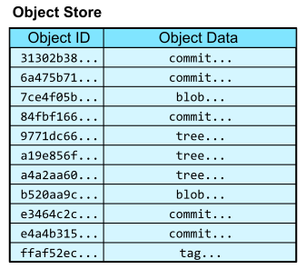
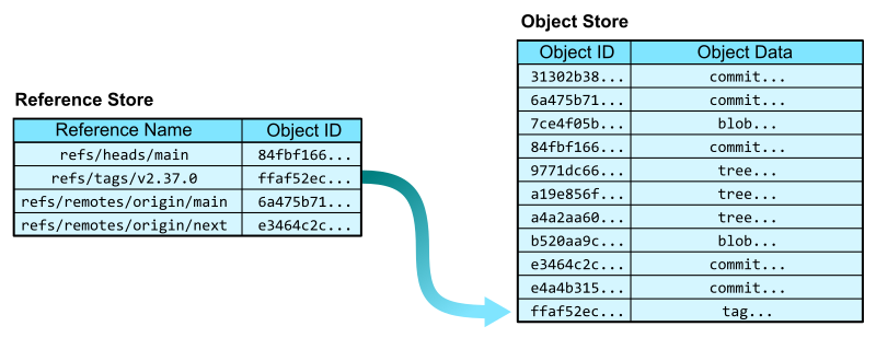
Registration is open for the following in-person AWS Summits that might be close to you in August and September: Canberra (August 31), Ottawa (September 8), New Delhi (September 9), and Mexico City (September 21–22), Bogotá (October 4), and Singapore (October 6).

AWS Community DayAWS Community DaysAWS Community Day events are community-led conferences that deliver a peer-to-peer learning experience, providing developers with a venue for them to acquire AWS knowledge in their preferred way: from one another.

In September, the AWS community will host events in the Bay Area, California (September 9) and in Arlington, Virginia (September 30). In October, you can join Community Days in Amersfoort, Netherlands (October 3), in Warsaw, Poland (October 14), and in Dresden, Germany (October 19).

That’s all for this week. Check back next Monday for another Week in Review! And maybe I’ll see you at the AWS Community Day here in the Bay Area!

Antje

This post is part of our Week in Review series. Check back each week for a quick roundup of interesting news and announcements from AWS!

Git’s database internals I: packed object store

Post Syndicated from Derrick Stolee original https://github.blog/2022-08-29-gits-database-internals-i-packed-object-store/

Developers collaborate using Git. It is the medium that allows us to share code, work independently on our own machines, and then finally combine our efforts into a common understanding. For many, this is done by following some well-worn steps and sticking to that pattern. This works in the vast majority of use cases, but what happens when we need to do something new with Git? Knowing more about Git’s internals helps when exploring those new solutions.

In this five-part blog post series, we will illuminate Git’s internals to help you collaborate via Git, especially at scale.

It might also be interesting because you love data structures and algorithms. That’s what drives me to be interested in and contribute to Git.

Git’s architecture follows patterns that may be familiar to developers, except the patterns come from a different context. Almost all applications use a database to persist and query data. When building software based on an application database system, it’s easy to get started without knowing any of the internals. However, when it’s time to scale your solution, you’ll have to dive into more advanced features like indexes and query plans.

The core idea I want to convey is this:

Git is the distributed database at the core of your engineering system.

Here are some very basic concepts that Git shares with application databases:

  1. Data is persisted to disk.
  2. Queries allow users to request information based on that data.
  3. The data storage is optimized for these queries.
  4. The query algorithms are optimized to take advantage of these structures.
  5. Distributed nodes need to synchronize and agree on some common state.

While these concepts are common to all databases, Git is particularly specialized. Git was built to store plain-text source code files, where most change are small enough to read in a single sitting, even if the codebase contains millions of lines. People use Git to store many other kinds of data, such as documentation, web pages, or configuration files.

While many application databases use long-running processes with significant amounts of in-memory caching, Git uses short-lived processes and uses the filesystem to persist data between executions. Git’s data types are more restrictive than a typical application database. These aspects lead to very specialized data storage and access patterns.

Today, let’s dig into the basics of what data Git stores and how it accesses that data. Specifically, we will learn about Git’s object store and how it uses packfiles to compress data that would otherwise contain redundant information.

Git’s object store

The most fundamental concepts in Git are Git objects. These are the “atoms” of your Git repository. They combine in interesting ways to create the larger structure. Let’s start with a quick overview of the important Git objects. Feel free to skip ahead if you know this, or you can dig deep into Git’s object model if you’re interested.

In your local Git repositories, your data is stored in the .git directory. Inside, there is a .git/objects directory that contains your Git objects.

$ ls .git/objects/
01  34  9a  df  info    pack

$ ls .git/objects/01/
12010547a8990673acf08117134bdc181bd735

$ ls .git/objects/pack/
multi-pack-index
pack-7017e6ce443801478cf19006fc5499ba1c4d2960.idx
pack-7017e6ce443801478cf19006fc5499ba1c4d2960.pack
pack-9f9258a8ffe4187f08a93bcba47784e07985d999.idx
pack-9f9258a8ffe4187f08a93bcba47784e07985d999.pack

The .git/objects directory is called the object store. It is a content-addressable data store, meaning that we can retrieve the contents of an object by providing a hash of those contents.

In this way, the object store is like a database table with two columns: the object ID and the object content. The object ID is the hash of the object content and acts like a primary key.

Table with columns labeled Object ID and Object Data

Upon first encountering content-addressable data stores, it is natural to ask, “How can we access an object by hash if we don’t already know its content?” We first need to have some starting points to navigate into the object store, and from there we can follow links between objects that exist in the structure of the object data.

First, Git has references that allow you to create named pointers to keys in the object database. The reference store mainly exists in the .git/refs/ directory and has its own advanced way of storing and querying references efficiently. For now, think of the reference store as a two-column table with columns for the reference name and the object ID. In the reference store, the reference name is the primary key.

Image showing how the Object ID table relates to the Object Store

Now that we have a reference store, we can navigate into the object store from some human-readable names. In addition to specifying a reference by its full name, such as refs/tags/v2.37.0, we can sometimes use short names, such as v2.37.0 where appropriate.

In the Git codebase, we can start from the v2.37.0 reference and follow the links to each kind of Git object.

  • The refs/tags/v2.37.0 reference points to an annotated tag object. An annotated tag contains a reference to another object (by object ID) and a plain-text message.
  • That tag’s object references a commit object. A commit is a snapshot of the worktree at a point in time, along with connections to previous versions. It contains links to parent commits, a root tree, as well as metadata, such as commit time and commit message.
  • That commit’s root tree references a tree object. A tree is similar to a directory in that it contains entries that link a path name to an object ID.
  • From that tree, we can follow the entry for README.md to find a blob object. Blobs store file contents. They get their name from the tree that points to them.

Image displaying hops through the object database in response to a user request.

From this example, we navigated from a ref to the contents of the README.md file at that position in the history. This very simple request of “give me the README at this tag” required several hops through the object database, linking an object ID to that object’s contents.

These hops are critical to many interesting Git algorithms. We will explore how the graph structure of the object store is used by Git’s algorithms in parts two through four. For now, let’s focus on the critical operation of linking an object ID to the object contents.

Object store queries

To store and access information in an application database, developers interact with the database using a query language such as SQL. Git has its own type of query language: the command-line interface. Git commands are how we interact with the Git object store. Since Git has its own structure, we do not get the full flexibility of a relational database. However, there are some parallels.

To select object contents by object ID, the git cat-file command will do the object lookup and provide the necessary information. We’ve already been using git cat-file -p to present “pretty” versions of the Git object data by object ID. The raw content is not always fit for human readers, with object IDs stored as raw hashes and not hexadecimal digits, among other things like null bytes. We can also use git cat-file -t to show the type of an object, which is discoverable from the initial few bytes of the object data.

To insert an object into the object store, we can write directly to a blob using git hash-object. This command takes file content and writes it into a blob in the object store. After the input is complete, Git reports the object ID of the written blob.

$ git hash-object -w --stdin
Hello, world!
af5626b4a114abcb82d63db7c8082c3c4756e51b

$ git cat-file -t af5626b4a114abcb82d63db7c8082c3c4756e51b
blob

$ git cat-file -p af5626b4a114abcb82d63db7c8082c3c4756e51b
Hello, world!

More commonly, we not only add a file’s contents to the object store, but also prepare to create new commit and tree objects to reference that new content. The git add command hashes new changes in the worktree and stores their blobs in the object store then writes the list of objects to a staging area known as the Git index. The git commit command takes those staged changes and creates trees pointing to all of the new blobs, then creates a new commit object pointing to the new root tree. Finally, git commit also updates the current branch to point to the new commit.

The figure below shows the process of creating several Git objects and finally updating a reference that happens when running git commit -a -m "Update README.md" when the only local edit is a change to the README.md file.

Image showing the process of creating several Git objects and updating references

We can do slightly more complicated queries based on object data. Using git log --pretty=format:<format-string>, we can make custom queries into the commits by pulling out “columns” such as the object ID and message, and even the committer and author names, emails, and dates. See the git log documentation for a full column list.

There are also some prebuilt formats ready for immediate use. For example, we can get a simple summary of a commit using git log --pretty=reference -1 <ref>. This query parses the commit at <ref> and provides the following information:

  • An abbreviated object ID.
  • The first sentence of the commit message.
  • The commit date in short form.
$ git log --pretty=reference -1 378b51993aa022c432b23b7f1bafd921b7c43835
378b51993aa0 (gc: simplify --cruft description, 2022-06-19)

Now that we’ve explored some of the queries we can make in Git, let’s dig into the actual storage of this data.

Compressed object storage: packfiles

Looking into the .git/objects directory again, we might see several directories with two-digit names. These directories then contain files with long hexadecimal names. These files are called loose objects, and the filename corresponds to the object ID of an object: the first two hexadecimal characters form the directory name while the rest form the filename. While the files themselves are compressed, there is not much interesting about querying these files, since Git relies on filesystem queries to satisfy most of these needs.

However, it does not take many objects before it is infeasible to store an entire Git repository using only loose objects. Not only does it strain the filesystem to have so many files, it is also inefficient when storing many versions of the same text file. Thus, Git’s packed object store in the .git/objects/pack/ directory forms a more efficient way to store Git objects.

Packfiles and pack-indexes

Each *.pack file in .git/objects/pack/ is called a packfile. Packfiles store multiple objects in compressed forms. Not only is each object compressed individually, they can also be compressed against each other to take advantage of common data.

At its simplest, a packfile contains a concatenated list of objects. It only stores the object data, not the object ID. It is possible to read a packfile to find objects by object ID, but it requires decompressing and hashing each object to compare it to the input hash. Instead, each packfile is paired with a pack-index file ending with .idx. The pack-index file stores the list of object IDs in lexicographical order so a quick binary search is sufficient to discover if an object ID is in the packfile, then an offset value points to where the object’s data begins within the packfile. The pack-index operates like a query index that speeds up read queries that rely on the primary key (object ID).

One small optimization is that a fanout table of 256 entries provides boundaries within the full list of object IDs based on their first byte. This reduces the time spent by the binary search, specifically by focusing the search on a smaller number of memory pages. This works particularly well because object IDs are uniformly distributed so the fanout ranges are well-balanced.

If we have a number of packfiles, then we could ask each pack-index in sequence to look up the object. A further enhancement to packfiles is to put several pack-indexes together in a single multi-pack-index, which stores the same offset data plus which packfile the object is in.

Lookups and prefixes work the same as in pack-indexes, except now we can skip the linear issue with many packs. You can read more about the multi-pack-index file and how it helps scale monorepo maintenance at GitHub.

Diffable object content

Packfiles also have a hyper-specialized version of row compression called deltification. Since read queries are only indexed by the object ID, we can perform extra compression on the object data part.

Git was built to store source code, which consists of plain-text files that are used as input to a compiler or interpreter to create applications. Git was also built to store many versions of this source code as it is changed by humans. This provides additional context about the kind of data typically stored in Git: diffable files with significant portions in common. If you’ve ever wondered why you shouldn’t store large binary files in Git repositories, this is the reason.

The field of software engineering has made it clear that it is difficult to understand applications in their entirety. Humans can grasp a very high-level view of an architecture and can parse small sections of code, but we cannot store enough information in our brains to grasp huge amounts of concrete code at once. You can read more about this in the excellent book, The Programmer’s Brain by Dr. Felienne Hermans.

Because of the limited size of our working memory, it is best to change code in small, well-documented iterations. This helps the code author, any code reviewers, and future developers looking at the code history. Between iterations, a significant majority of the code remains fixed while only small portions change. This allows Git to use difference algorithms to identify small diffs between the content of blob objects.

There are many ways to compute a difference between two blobs. Git has several difference algorithms implemented which can have drastically different results. Instead of focusing on unstructured differences, I want to focus on differences between structured object data. Specifically, tree objects usually change in small ways that are easy to compress.

Tree diffs

Git’s tree objects can also be compared using a difference algorithm that is aware of the structure of tree entries. Each tree entry stores a mode (think Unix file permissions), an object type, a name, and an object ID. Object IDs are for all intents and purposes random, but most edits will change a file without changing its mode, type, or name. Further, large trees are likely to have only a few entries change at a time.

For example, the tip commit at any major Git release only changes one file: the GIT-VERSION-GEN file. This means also that the root tree only has one entry different from the previous root tree:

$ git diff v2.37.0~1 v2.37.0
diff --git a/GIT-VERSION-GEN b/GIT-VERSION-GEN
index 120af376c1..b210b306b7 100755
--- a/GIT-VERSION-GEN
+++ b/GIT-VERSION-GEN
@@ -1,7 +1,7 @@
 #!/bin/sh

 GVF=GIT-VERSION-FILE
-DEF_VER=v2.37.0-rc2
+DEF_VER=v2.37.0

 LF='
 '

$ git cat-file -p v2.37.0~1^{tree} >old
$ git cat-file -p v2.37.0^{tree} >new

$ diff old new
13c13
< 100755 blob 120af376c147799e6c0069bac1f61709a0286cd6  GIT-VERSION-GEN
---
> 100755 blob b210b306b7554f28dc687d1c503517d2a5f87082  GIT-VERSION-GEN

Once we have an algorithm that can compute diffs for Git objects, the packfile format can take advantage of that.

Delta compression

The packfile format begins with some simple header information, but then it contains Git object data concatenated together. Each object’s data starts with a type and a length. The type could be the object type, in which case the content in the packfile is the full object content (subject to DEFLATE compression). The object’s type could instead be an offset delta, in which case the data is based on the content of a previous object in the packfile.

An offset delta begins with an integer offset value pointing to the relative position of a previous object in the packfile. The remaining data specifies a list of instructions which either instruct how to copy data from the base object or to write new data chunks.

Thinking back to our example of the root tree for Git’s v2.37.0 tag, we can store that tree as an offset delta to the previous root tree by copying the tree up until the object ID 120af37..., then write the new object ID b210b30..., and finally copy the rest of the previous root tree.

Keep in mind that these instructions are also DEFLATE compressed, so the new data chunks can also be compressed similarly to the base object. For the example above, we can see that the root tree for v2.37.0 is around 19KB uncompressed, 14KB compressed, but can be represented as an offset delta in only 50 bytes.

$ git rev-parse v2.37.0^{tree}
a4a2aa60ab45e767b52a26fc80a0a576aef2a010

$ git cat-file -s v2.37.0^{tree}
19388

$ ls -al .git/objects/a4/a2aa60ab45e767b52a26fc80a0a576aef2a010
-r--r--r--   1 ... ... 13966 Aug  1 13:24 a2aa60ab45e767b52a26fc80a0a576aef2a010

$ git rev-parse v2.37.0^{tree} | git cat-file --batch-check="%(objectsize:disk)"
50

Also, an offset delta can be based on another object that is also an offset delta. This creates a delta chain that requires computing the object data for each object in the list. In fact, we need to traverse the delta links in order to even determine the object type.

For this reason, there is a cost to storing objects efficiently this way. At read time, we need to do a bit extra work to materialize the raw object content Git needs to parse to satisfy its queries. There are multiple ways that Git tries to optimize this trade-off.

One way Git minimizes the extra work when parsing delta chains is by keeping the delta-chains short. The pack.depth config value specifies an upper limit on how long delta chains can be while creating a packfile. The default limit is 50.

When writing a packfile, Git attempts to use a recent object as the base and order the delta chain in reverse-chronological order. This allows the queries that involve recent objects to have minimum overhead, while the queries that involve older objects have slightly more overhead.

However, while thinking about the overhead of computing object contents from a delta chain, it is important to think about what kind of resources are being used. For example, to compute the diff between v2.37.0 and its parent, we need to load both root trees. If these root trees are in the same delta chain, then that chain’s data on disk is smaller than if they were stored in raw form. Since the packfile also places delta chains in adjacent locations in the packfile, the cost of reading the base object and its delta from disk is almost identical to reading just the base object. The extra overhead of some CPU during the parse is very small compared to the disk read. In this way, reading multiple objects in the same delta chain is faster than reading multiple objects across different chains.

In addition, some Git commands query the object store in such a way that we are very likely to parse multiple objects in the same delta chain. We will cover this more in part III when discussing file history queries.

In addition to persisting data efficiently to disk, the packfile format is also critical to how Git synchronizes Git object data across distributed copies of the repository during git fetch and git push. We will learn more about this in part IV when discussing distributed synchronization.

Packfile maintenance

In order to take advantage of packfiles and their compressed representation of Git objects, Git needs to actually write these packfiles. It is too expensive to create a packfile for every object write, so Git batches the packfile write into certain commands.

You could roll your own packfile using git pack-objects and create a pack-index for it using git index-pack. However, you instead might want to recompute a new packfile containing your entire object store using git repack -a or git gc.

As your repository grows, it becomes more difficult to replace your entire object store with a new packfile. For starters, you need enough space to store two copies of your Git object data. In addition, the computation effort to find good delta compression is very expensive and demanding. An optimal way to do delta compression takes quadratic time over the number objects, which is quickly infeasible. Git uses several heuristics to help with this, but still the cost of repacking everything all at once can be more than we are willing to spend, especially if we are just a client repository and not responsible for serving our Git data to multiple users.

There are two primary ways to update your object store for efficient reads without rewriting the entire object store into a new packfile. One is the geometric repacking option where you can run git repack --geometric to repack only a portion of packfiles until the resulting packfiles form a geometric sequence. That is, each packfile is some fixed multiple smaller than the next largest one. This uses the multi-pack-index to keep logarithmic performance for object lookups, but will occasionally tip over to repack all of the object data. That “tip over” moment only happens when the repository doubles in size, which does not happen very often.

Another approach to reducing the amount of work spent repacking is the incremental repack task in the git maintenance command. This task collects packfiles below a fixed size threshold and groups them together, at least until their total size is above that threshold. The default threshold is two gigabytes. This task is used by default when you enable background maintenance with the git maintenance start command. This also uses the multi-pack-index to keep fast lookups, but also will not rewrite the entire object store for large repositories since once a packfile is larger than the threshold it is not considered for repacking. The storage is slightly inefficient here, since objects in newer packfiles could be stored as deltas to objects in those fixed packs, but the simplicity in avoiding expensive repository maintenance is worth that slight overhead.

If you’re interested in keeping your repositories well maintained, then think about these options. You can always perform a full repack that recomputes all delta chains using git repack -adf at any time you are willing to spend that upfront maintenance cost.

What could Git learn from other databases?

Now that we have some understanding about how Git stores and accesses packed object data, let’s think about features that exist in application database systems that might be helpful here.

One thing to note is that there are no B-trees to be found! Almost every database introduction talks about how B-trees are used to efficiently index data in a database table. Why are they not present here in Git?

The main reason Git does not use B-trees is because it doesn’t do “live updating” of packfiles and pack-indexes. Once a packfile is written, it is static until it is replaced by another packfile containing its objects. That packfile is also not accessed by Git processes until its pack-index is completely written.

In this world, objects are dynamically added to the object store by adding new loose object files (such as in git add or git commit) or by adding new packfiles (such as in git fetch). If a packfile has fixed content, then we can do the most space-and-time efficient index: a binary search tree. Specifically, performing binary search on the list of object IDs in a pack-index is very efficient. It’s not an exact binary search because there is an initial fan-out table for the first byte of the object ID. It’s kind of like a rooted binary tree, except the root node has 256 children instead of only two.

B-trees excel when data is being inserted or removed from the tree. Being able to track those modifications with minimal modifications to the overall tree structure is critical for an application database serving many concurrent requests.

Git does not currently have the capability to update a packfile in real time without shutting down concurrent reads from that file. Such a change could be possible, but it would require updating Git’s storage significantly. I think this is one area where a database expert could contribute to the Git project in really interesting ways.

Another difference between Git and most database systems is that Git runs as short-lived processes. Typically, we think of the database as a process that has data cached in memory. We send queries to the existing process and it returns results and keeps running. Instead, Git starts a new process with every “query” and relies on the filesystem for persisted state. Git also relies on the operating system to cache the disk pages during and between the processes. Expert database systems tell the kernel to stop managing disk pages and instead the database manages the page cache since it knows its usage needs better than a general purpose operating system could predict.

What if Git had a long-running daemon that could satisfy queries on-demand, but also keep that in-memory representation of data instead of needing to parse objects from disk every time? Although the current architecture of Git is not well-suited to this, I believe it is an idea worth exploring in the future.

Come back tomorrow for more!

In the next part of this blog series, we will explore how Git commit history queries use the structure of Git commits to present interesting information to the user. We’ll also explore the commit-graph file and how it acts as a specialized query index for these commands.

I’ll also be speaking at Git Merge 2022 covering all five parts of this blog series, so I look forward to seeing you there!

Open sourcing our fork of PgBouncer

Post Syndicated from Justin Kwan original https://blog.cloudflare.com/open-sourcing-our-fork-of-pgbouncer/

Open sourcing our fork of PgBouncer

Open sourcing our fork of PgBouncer

Cloudflare operates highly available Postgres production clusters across multiple data centers, supporting the transactional workloads of our core service offerings such as our DNS Resolver, Firewall, and DDoS Protection.

Multiple PgBouncer instances sit at the front of the gateway layer per each cluster, acting as a TCP proxy that provides Postgres connection pooling. PgBouncer’s pooling enables upstream applications to connect to Postgres, without having to constantly open and close connections (expensive) at the database level, while also reducing the number of Postgres connections used. Each tenant acquires client-side connections from PgBouncer instead of Postgres directly.

Open sourcing our fork of PgBouncer

PgBouncer will hold a pool of maximum server-side connections to Postgres, allocating those across multiple tenants to prevent Postgres connection starvation. From here, PgBouncer will forward backend queries to HAProxy, which load balances across Postgres primary and read replicas.

As an intern at Cloudflare I got to work on improving how our database clusters behave under load and open source the resulting code.

We run our Postgres infrastructure in non-containerized, bare metal environments which consequently leads to multitenant resource contention between Postgres users. To enforce stricter tenant performance isolation at the database level (CPU time utilized, memory consumption, disk IO operations), we’d like to configure and enforce connection limits per user and connection pool at PgBouncer.

To do that we had to add features and fix bugs in PgBouncer. Rather than continue to maintain a private fork we are open sourcing our code for others to use.

Authentication Rejection

The PgBouncer connection pooler offers options to enforce server connection pool size limits (effective concurrency) per user via static configuration. However, an authentication bug upstream prevented these features from correctly working when Postgres was set to use HBA authentication. Administrators who sensibly use server-side authentication could not take advantage of these user-level features.

This ongoing issue has also been experienced by others in the open-source community:

https://github.com/pgbouncer/pgbouncer/issues/484
https://github.com/pgbouncer/pgbouncer/issues/596

Root Cause

PgBouncer needs a Postgres user’s password when proxying submitted queries from client connection to a Postgres server connection. PgBouncer will fetch a user’s Postgres password defined in userlist.txt (auth_file) when a user first logs in to compare against the provided password. However, if the user is not defined in userlist.txt, Pgbouncer will fetch their password from the Postgres pg_shadow system view for comparison. This password will be used when PgBouncer subsequently forwards queries from this user to Postgres. The same applies when Postgres is configured to use HBA authentication.

Following serious debugging efforts and time spent in GDB, we found that multiple user objects are typically created for a single real user: via configuration loading from the [users] section and upon the user’s first login. In PgBouncer, any users requiring a shadow auth query would be stored under their respective database struct instance, whereas any user with a password defined in userlist.txt would be stored globally. Because the non-authenticated user already existed in memory after being parsed from the [users] section, PgBouncer assumed that the user was defined in userlist.txt, where the shadow authentication query could be skipped. It would not bother to fetch and set the user’s password upon first login, resulting in an empty user password. This is why subsequent queries submitted by the user would be rejected with authentication failure at Postgres.

To solve this, we simplified the code to globally store all users in one place rather than store different types of users (requiring different methods of authentication) in a disaggregated fashion per database or globally. Also, rather than assuming a user is authenticated if they merely exist, we keep track of whether the user requires authentication via auth query or from fetching their password from userlist.txt. This depends on how they were created.

We saw the value in troubleshooting and fixing these issues; it would unlock an entire class of features in PgBouncer for our use cases, while benefiting many in the open-source community.

New Features

We’ve also done work to implement and support additional features in PgBouncer to enforce stricter tenant performance isolation.

Previously, PgBouncer would only prevent tenants from exceeding preconfigured limits, not particularly helpful when it’s too late and a user is misbehaving or already has too many connections. PgBouncer now supports enforcing or shrinking per user connection pool limits at runtime, where it is most critically needed to throttle tenants who are issuing a burst of expensive queries, or are hogging connections from other tenants. We’ve also implemented new administrative commands to throttle the maximum connections per user or per pool at runtime.

PgBouncer also now supports statically configuring and dynamically enforcing connection limits per connection pool. This feature is extremely important in order to granularly throttle a tenant’s misbehaving connection pool without throttling and reducing availability on its other non-misbehaving pools.

PgBouncer Configuration
[users]
dns_service_user = max_user_connections=60
firewall_service_user = max_user_connections=80
[pools]
user1.database1 = pool_size=90
PgBouncer Runtime Commands
SET USER dns_service_user = ‘max_user_connections=40’;
SET POOL dns_service_user.dns_db = ‘pool_size=30’;

These new features required major refactoring around how PgBouncer stores users, databases weakly referenced and stored passwords of different users, and how we enforce killing server side connections while still in use.

Conclusion

We are committed to improving PgBouncer in open source and contributing all of our features to benefit the wider community. If you are interested, please consider contributing to our open source PgBouncer fork. After all, it is the community that makes PgBouncer possible!

Introducing Trilogy: a new database adapter for Ruby on Rails

Post Syndicated from Matthew Draper original https://github.blog/2022-08-25-introducing-trilogy-a-new-database-adapter-for-ruby-on-rails/

We’ve open sourced the database adapter we use at GitHub to connect Ruby on Rails and Active Record clients to MySQL-compatible database servers.

Trilogy is a client library for MySQL-compatible database servers, designed for performance, flexibility, and ease of embedding. We released Trilogy, with its Ruby-native wrapper, in December, and have now rounded out the set with the release of activerecord-trilogy-adapter, an Active Record adapter that allows a Ruby on Rails application to use Trilogy in place of the built-in mysql2-based adapter.

Why does Trilogy exist?

The Trilogy library is specifically designed to perform efficiently when embedded in environments like the Ruby VM, which benefits from special handling of blocking syscalls, and conscious use of dynamic memory allocation. It also aims to provide strong portability and compatibility, using a custom implementation of the network protocol to minimize dependencies needed for compilation.

After starting off on the original mysql gem, GitHub switched to mysql2 in 2011, gaining performance and reliability. But over the following years, we found it was still not quite meeting our needs. Trilogy was initially developed by Hailey Somerville and Brian Lopez to further improve GitHub’s performance and reliability, and has been backing all of our Rails monolith’s query activity since 2015. (The name is a pun: it’s the third adapter GitHub has used, and it’s used to query sequel.)

Open sourcing this adapter is the culmination of a long term effort, primarily championed first by Aaron Patterson and then by Eileen M. Uchitelle, to extract valuable database-communication behavior we’d collected and upstream it into other layers of Active Record—most recently, deferred connection verification and automatic reconnection.

Should you use Trilogy?

Compared to the mysql2 gem, Trilogy avoids a dependency on the libmariadb / libmysqlclient library, which can simplify gem installation and eliminate version mismatch issues, and minimizes the number of times data must be copied in memory when building and parsing network packets. It should simplify gem installation and be more efficient under heavy query loads.

Trilogy is thoroughly production-tested to work well for our applications, but there may be protocol features it doesn’t support (yet?) that other database configurations might require. For that reason, while we do encourage other Rails applications to try using Trilogy to interface with their MySQL-compatible database servers, it would be prudent to check things out in a staging environment first. Other than that, it should be a drop-in compatible change.

The Trilogy adapter is currently only compatible with the version of Rails that we use to run GitHub: the in-development main branch of rails/rails. After Active Record 7.1.0 is released, we will maintain a release that is compatible with the current supported release series.

Trilogy is a strong option when connecting to a MySQL-compatible database server, and we would love to hear from you if you give it a try.

Pushing Open-Source Security Forward: Insights From Black Hat 2022

Post Syndicated from Jesse Mack original https://blog.rapid7.com/2022/08/19/pushing-open-source-security-forward-insights-from-black-hat-2022/

Pushing Open-Source Security Forward: Insights From Black Hat 2022

Open-source security has been a hot topic in recent years, and it’s proven to be something of a double-edged sword. On the one hand, there’s an understanding of the potential that open-source tools hold for democratizing security, making industry best practices accessible to more organizations and helping keep everyone’s data better protected from attackers. On the other hand, open-source codebases have been the subject of some of the most serious and high-impact vulnerabilities we’ve seen over the past 12 months, namely Log4Shell and Spring4Shell.

While the feeling around open-source understandably wavers between excitement and trepidation, one thing is for sure: Open-source frameworks are here to stay, and it’s up to us to ensure they deliver on their potential and at the same time remain secure.

The future of open-source was common theme at Black Hat 2022, and two members of the Rapid7 research team — Lead Security Research Spencer McIntyre and Principal Security Researcher Curt Barnard — shined a light on the work they’ve been doing to improve and innovate with open-source tools. Here’s a look at their presentations from Black Hat, and how their efforts are helping push open-source security forward.

A more powerful Metasploit

Spencer, whose work focuses primarily on Rapid7’s widely used attacker emulation and penetration testing tool Metasploit, shared the latest and greatest improvements he and the broader team have made to the open-source framework in the past year. The upgrades they’ve made reflect a reality that security pros across the globe are feeling everyday: The perimeter is disappearing.

In a threat environment shaped by ransomware, supply chain attacks, and widespread vulnerabilities like Log4Shell, bad actors are increasingly stringing together complex attack workflows leveraging multiple vulnerabilities. These techniques allow adversaries to go from outside to within an organization’s network more quickly and easily than ever before.

The updates Spencer and team have made to Metasploit are intended to help security teams keep up with this shift, with more modern, streamlined workflows for testing the most common attack vectors. These recent improvements to Metasploit include:

Credential capturing: Credential capture is a key component of the attacker emulation toolkit, but previously, the process for this in Metasploit involved spinning up 13 different modules and managing and specifying configurations for each. Now, Metasploit offers a credential capture plugin that lets you configure all options from a single start/stop command, eliminating redundant work.

User interface (UI) optimization: URLs are commonly used to identify endpoints — particularly web applications — during attacker emulation. Until now, Metasploit required users to manually specify quite a few components when using URLs. The latest update to the Metasploit UI understands a URL’s format, so users can copy and paste them from anywhere, even right from their browser.

Payloadless session capabilities: When emulating attacks, exploits typically generate Meterpreter payloads, making them easy to spot for many antivirus and EDR solutions — and reducing their effectiveness for security testing. Metasploit now lets you run post-exploitation actions and operations without needing a payload. You can tunnel modules through SSH sessions or create a WinRM session for any Metasploit module compatible with the shell session type, removing the need for a payload like reverse shell or Meterpreter.

SMB server support: Metasploit Version 6 included SMB 3 server support, but only for client modules, which was limiting for users who were working with modern Windows targets that had disabled SMB 3 client support. Now, SMB 3 is available in all SMB server modules, so you can target modern Windows environments and have them fetch (often payload) files from Metasploit. This means you don’t need to install and configure an external service to test for certain types of vulnerabilities, including PrintNightmare.

Defaultinator: Find default credentials faster

Metasploit is at the heart of Rapid7’s commitment to open-source security, but we’re not stopping there. In addition to continually improving Metasploit, our research team works on new open-source projects that help make security more accessible for all. The latest of those is Defaultinator, a new tool that Curt Barnard announced the release of in his Black Hat Arsenal talk this year. (Curt also joined our podcast, Security Nation, to preview the announcement — check out that episode if you haven’t yet!)

Defaultinator is an open-source tool for looking up default usernames and passwords, providing an easy-to-search data repository in which security pros can query these commonly used credentials to find and eliminate them from their environment. This capability is becoming increasingly important for security teams, for a few key reasons:

  • Some commonly used pieces of hardware in IT environments come with default credentials that could give attackers an easily exploitable method of network access. Curt gave the example of the Raspberry Pi microcontroller board, which always comes with the username “pi” and password “raspberry” for initial login — a security flaw that resulted in a 10 CVSS vulnerability published in 2021.
  • Meanwhile, IoT devices have been proliferating, and many of these manufacturers don’t have security best practices at the front of their mind. That means hardcoded default credentials for first-time logins are common in this type of tool.
  • Many software engineers (Curt included) spend a lot of time in Stack Overflow, and many of the code snippets found there contain example usernames and passwords. If you aren’t careful when copying and pasting, default credentials could make their way into your production environment.

With a whopping 54 CVEs for hardcoded usernames and passwords released just in 2022 so far (by Curt’s count), security pros are in need of a fast, accurate way to audit for default credentials. But until now, the tools for these kinds of audits just haven’t been out there, let alone widely available.

That’s why it was so important to make Defaultinator, the first tool of its kind for querying default usernames and passwords, an open-source solution — to ensure broad accessibility and help as many defenders as possible. Defaultinator offers an API search-based utility or a web-based user interface if you prefer not to interact with the API. It runs in Docker, and the quickstart repository on Github takes just four lines of code to get up and running.

Watch the replays of Spencer’s and Curt’s presentations, as well as other great sessions from Black Hat 2022, at our replay page.

Additional reading:

NEVER MISS A BLOG

Get the latest stories, expertise, and news about security today.

OCSF: Working Together to Standardize Data

Post Syndicated from Rapid7 original https://blog.rapid7.com/2022/08/10/ocsf-working-together-to-standardize-data/

OCSF: Working Together to Standardize Data

Teams spend a lot of time normalizing data before any analysis, investigation, or response can begin. It’s an unacceptable burden for you. And its days are finally numbered.

Rapid7 and other security vendors are collaborating on an Open Cybersecurity Schema Framework (OCSF), an open standard for both data producers and users to adopt. Much like the MITRE Att@ck Framework, common language and understanding change everything.

OCSF, includes contributions from 17 leading cybersecurity and technology organizations: AWS, Cloudflare, CrowdStrike, DTEX, IBM Security, IronNet, JupiterOne, Okta, Palo Alto Networks, Rapid7, Salesforce, Securonix, Splunk, Sumo Logic, Tanium, Trend Micro, and Zscaler.

OCSF is an open standard that can be adopted in any environment, application, or solution provider and fits with existing security standards and processes. As cybersecurity solution providers incorporate OCSF standards into their products, security data normalization will become simpler, allowing teams to focus on analyzing data, identifying threats, and stopping attackers before they cause damage.

“We, as security vendors, need to do right by the security teams who work tirelessly to protect not only their organizations, but the greater community, against a constantly evolving array of threats,” said Sam Adams, Vice President of Detection and Response, Rapid7. “A step towards that is standardizing the data on which these teams rely. If we can minimize the complexity of using security data from disparate sources, we can save security professionals millions of hours every year. Rapid7 has a proud history of supporting the open-source community. We are thrilled to join our peers who share this belief and build a solution that will break down data silos, removing a heavy burden that hinders security teams’ efforts to stay ahead of threats.”

Data holds the key

The key to efficiently detecting and rapidly responding to today’s threats and attacks is data and how you use that data. It’s mission-critical for security teams to evaluate data from various sources (e.g. the endpoint, threat intelligence feeds, logs, etc.), coordinating with a myriad of security tools and solutions. In a recent study, SOC Modernization and the Role of XDR, eight in 10 organizations said they collect, process, and analyze security operations data from more than 10 sources. While it might sound like a lot, survey respondents actually want to use more data, in order to keep up with the evolving attack surface.

As the industry comes together to unburden security teams of the work required to collect and normalize data, Rapid7 will be rolling out support for OCSF, starting with InsightIDR, our joint SIEM and XDR solution. Look for updates on OCSF support in the coming months!

Additional reading:

NEVER MISS A BLOG

Get the latest stories, expertise, and news about security today.

AWS Week in Review – August 8, 2022

Post Syndicated from Steve Roberts original https://aws.amazon.com/blogs/aws/aws-week-in-review-august-8-2022/

As an ex-.NET developer, and now Developer Advocate for .NET at AWS, I’m excited to bring you this week’s Week in Review post, for reasons that will quickly become apparent! There are several updates, customer stories, and events I want to bring to your attention, so let’s dive straight in!

Last Week’s launches
.NET developers, here are two new updates to be aware of—and be sure to check out the events section below for another big announcement:

Tiered pricing for AWS Lambda will interest customers running large workloads on Lambda. The tiers, based on compute duration (measured in GB-seconds), help you save on monthly costs—automatically. Find out more about the new tiers, and see some worked examples showing just how they can help reduce costs, in this AWS Compute Blog post by Heeki Park, a Principal Solutions Architect for Serverless.

Amazon Relational Database Service (RDS) released updates for several popular database engines:

  • RDS for Oracle now supports the April 2022 patch.
  • RDS for PostgreSQL now supports new minor versions. Besides the version upgrades, there are also updates for the PostgreSQL extensions pglogical, pg_hint_plan, and hll.
  • RDS for MySQL can now enforce SSL/TLS for client connections to your databases to help enhance transport layer security. You can enforce SSL/TLS by simply enabling the require_secure_transport parameter (disabled by default) via the Amazon RDS Management console, the AWS Command Line Interface (AWS CLI), AWS Tools for PowerShell, or using the API. When you enable this parameter, clients will only be able to connect if an encrypted connection can be established.

Amazon Elastic Compute Cloud (Amazon EC2) expanded availability of the latest generation storage-optimized Is4gen and Im4gn instances to the Asia Pacific (Sydney), Canada (Central), Europe (Frankfurt), and Europe (London) Regions. Built on the AWS Nitro System and powered by AWS Graviton2 processors, these instance types feature up to 30 TB of storage using the new custom-designed AWS Nitro System SSDs. They’re ideal for maximizing the storage performance of I/O intensive workloads that continuously read and write from the SSDs in a sustained manner, for example SQL/NoSQL databases, search engines, distributed file systems, and data analytics.

Lastly, there’s a new URL from AWS Support API to use when you need to access the AWS Support Center console. I recommend bookmarking the new URL, https://support.console.aws.amazon.com/, which the team built using the latest architectural standards for high availability and Region redundancy to ensure you’re always able to contact AWS Support via the console.

For a full list of AWS announcements, be sure to keep an eye on the What’s New at AWS page.

Other AWS News
Here’s some other news items and customer stories that you may find interesting:

AWS Open Source News and Updates – Catch up on all the latest open-source projects, tools, and demos from the AWS community in installment #123 of the weekly open source newsletter.

In one recent AWS on Air livestream segment from AWS re:MARS, discussing the increasing scale of machine learning (ML) models, our guests mentioned billion-parameter ML models which quite intrigued me. As an ex-developer, my mental model of parameters is a handful of values, if that, supplied to methods or functions—not billions. Of course, I’ve since learned they’re not the same thing! As I continue my own ML learning journey I was particularly interested in reading this Amazon Science blog on 20B-parameter Alexa Teacher Models (AlexaTM). These large-scale multilingual language models can learn new concepts and transfer knowledge from one language or task to another with minimal human input, given only a few examples of a task in a new language.

When developing games intended to run fully in the cloud, what benefits might there be in going fully cloud-native and moving the entire process into the cloud? Find out in this customer story from Return Entertainment, who did just that to build a cloud-native gaming infrastructure in a few months, reducing time and cost with AWS services.

Upcoming events
Check your calendar and sign up for these online and in-person AWS events:

AWS Storage Day: On August 10, tune into this virtual event on twitch.tv/aws, 9:00 AM–4.30 PM PT, where we’ll be diving into building data resiliency into your organization, and how to put data to work to gain insights and realize its potential, while also optimizing your storage costs. Register for the event here.

AWS SummitAWS Global Summits: These free events bring the cloud computing community together to connect, collaborate, and learn about AWS. Registration is open for the following AWS Summits in August:

AWS .NET Enterprise Developer Days 2022 – North America: Registration for this free, 2-day, in-person event and follow-up 2-day virtual event opened this past week. The in-person event runs September 7–8, at the Palmer Events Center in Austin, Texas. The virtual event runs September 13–14. AWS .NET Enterprise Developer Days (.NET EDD) runs as a mini-conference within the DeveloperWeek Cloud conference (also in-person and virtual). Anyone registering for .NET EDD is eligible for a free pass to DeveloperWeek Cloud, and vice versa! I’m super excited to be helping organize this third .NET event from AWS, our first that has an in-person version. If you’re a .NET developer working with AWS, I encourage you to check it out!

That’s all for this week. Be sure to check back next Monday for another Week in Review roundup!

— Steve
This post is part of our Week in Review series. Check back each week for a quick roundup of interesting news and announcements from AWS!

Building and using Managed Components with WebCM

Post Syndicated from Yo'av Moshe original https://blog.cloudflare.com/building-using-managed-components-webcm/

Building and using Managed Components with WebCM

Building and using Managed Components with WebCM

Managed Components are here to shake up the way third-party tools integrate with websites. Two months ago we announced that we’re open sourcing parts of the most innovative technologies behind Cloudflare Zaraz, making them accessible and usable to everyone online. Since then, we’ve been working hard to make sure that the code is well documented and all pieces are fun and easy to use. In this article, I want to show you how Managed Components can be useful for you right now, if you manage a website or if you’re building third-party tools. But before we dive in, let’s talk about the past.

Third-party scripts are a threat to your website

For decades, if you wanted to add an analytics tool to your site, a chat widget, a conversion pixel or any other kind of tool – you needed to include an external script. That usually meant adding some code like this to your website:

<script src=”https://example.com/script.js”></script>

If you think about it – it’s a pretty terrible idea. Not only that you’re now asking the browser to connect to another server, fetch and execute more JavaScript code – you’re also completely giving up the control on your website. How much do you really trust this script? And how much do you trust that the script’s server wasn’t hacked, or will never get hacked in the future? In the previous blog post we showed how including one script usually results in more network calls, hogging the browser and slowing everything down. But the worst thing about these scripts is that they are completely unrestricted: JavaScript code running in the browser can hijack users, steal their credentials or credit card information, use their devices to mine cryptocurrencies, manipulate your website, leak PII, and more. Since the code in those scripts is usually minified, it’s practically impossible for you to read it and figure out what it’s doing.

Managed Components change all that. Like apps on your phone, they’re built around a permissions system. You decide if you allow a component to connect to a remote server, if you allow it to use cookies, to run code, to inject a widget to pages and more. Unlike the world of minified external scripts, it is a framework that promotes transparency. Website owners can toggle permissions on and off, and if a Managed Component wasn’t granted a permission, it will not have access to the relevant API.

But Managed Components do more than wrapping the current system with permissions – they also provide functionality that was never available before: making server-side connections, caching information, using a key-value store, manipulating responses before they are handed to the browser and more. The core of this functionality comes from the ability to execute code outside the browser. Freeing the browser from running code that was previously executed in the browser, means that your website can become approximately 40% faster. It also results in a smaller attack surface in case your tool’s vendor gets hacked.

All of this is possible thanks to the new Managed Components API. We designed it together with vendors, to make sure you can use them to write any tool, while keeping performance, security and privacy a top priority. At its core, a Managed Component is just a JavaScript module, and so every JavaScript developer should feel right at home when building one. Check out the two examples in our previous blog post to see how they actually look like, or see some Managed Components we already open sourced on GitHub.

WebCM is the open source Component Manager

When tools are loaded with a <script> tag, their code is executed by the browser. Since Managed Components don’t run in the browser, their code needs to be executed somewhere else. This is the Component Manager. We designed the APIs around Managed Components deliberately to not be tied to a specific Component Manager, and in fact, there are already two in the world: Cloudflare Zaraz, and WebCM.

WebCM, Web-based Component Manager, is our open source reference implementation of a Component Manager. If you run a website, you can use WebCM today to run Managed Components on your website, even if you’re not a Cloudflare user. If you want to create a Managed Component, you can use it like an SDK.

Over the last few months, we’ve been helping vendors to write their own Managed Components, and we will continue to do so. We open sourced WebCM to ensure that Managed Components are a technology of the Web as a whole. Everyone should be able to use WebCM to load and create Managed Components. Let’s see how to use it!

Getting started with WebCM in 5 minutes

Getting started with WebCM is easier than you think. Because WebCM works like a proxy, you can use it regardless of how your website is built. In a new folder, create a simple HTML file and call it index.html:

<!DOCTYPE html>
<html lang=”en”>
  <head>
	<meta charset="UTF-8">
	<title>My Website</title>
  </head>
  <body>
    	<h1>WebCM test website</h1>  
  </body>
</html>

Let’s serve this file by launching an HTTP serve in the same folder:

You can use Node.js:

npx http-server -p 8000

You can use Python:

python3 -m http.server

Or anything else that would serve our HTML file on http://localhost:8000/index.html.

Next, create a configuration file for WebCM. In a new directory, create a file called webcm.config.ts.

export default {
  components: [
    {
      name: 'demo',
      permissions: [
        'access_client_kv',
        'provide_server_functionality',
        'provide_widget',
        'serve_static_files',
        'client_network_requests',
      ],
    },
  ],
  target: 'http://127.0.0.1:8000',
  hostname: 'localhost',
  trackPath: '/webcm/track',
  ecommerceEventsPath: '/webcm/ecommerce',
  clientEventsPath: '/webcm/system',
  port: 8080
}

Let’s go over this configuration file:

  • components is an array that lists all the Managed Components you want to load. For now, we will load the demo component. Note that all we needed was to specify “demo”, and WebCM will go and get it from NPM for us. Other Managed Components are available on NPM too, and you can install components from other sources too. For each component, we’re defining what permissions we are giving it. You can read more about the permissions in the specifications. If we try to add the component without granting it its required permissions, WebCM will alert us.
  • target is where our origin HTTP server runs. In the previous step, we set it to run on port 8000.
  • port is the port under which WebCM will serve our website.
  • hostname is the host WebCM will bind to.
  • trackPath, clientEventsPath, ecommerceEventsPath are paths that WebCM will use to send events from the browser to its backend. We can leave these paths as they are for now, and will see how they’re used later.

! Note: Node version 17 or higher is needed for the next section

While keeping your HTTP server running, and in the same directory as webcm.config.ts, run npx webcm. Node will fetch WebCM and start it for you, and WebCM will read the configuration. First, it will fetch the required components to a components folder. When done, it will start another server that proxies your origin.

If you open http://localhost:8080/index.html in your browser now, you’d see the same page you saw at http://localhost:8000/index.html. While the pages might look similar, the one running on port 8080 has our demo Managed Component running. Moving your mouse and clicking around the page should result in messages being printed in your WebCM terminal, showing that the component was loaded and that it is receiving data. You will also notice that the page now displays a simple weather widget – this a Managed Component Widget that got appended to your page. The weather information was fetched without the browser needing to contact any additional server, and WebCM can cache that information to make sure it is served fast. Lastly, if you go to http://localhost:8080/webcm/demo/cheese, you’ll see that the component is serving a static image of a cheese. This is an example of how Managed Components can expose new endpoints on your servers, if you allow them.

The Demo Component, like its name suggests, is just a demo. We use it to showcase and test the Managed Components APIs. What if we want to add a real Managed Component to our site? Google Analytics is used by more than half of the websites on the internet, so let’s see how we edit our webcm.config.ts file to load it.

export default {
  components: [
    {
      name: 'demo',
      permissions: [
        'access_client_kv',
        'provide_server_functionality',
        'provide_widget',
        'serve_static_files',
        'client_network_requests',
      ],
    },
    {
      name: 'google-analytics',
      settings: { 'tid': 'UA-XXXXXX' },
      permissions: [
        'access_client_kv',
      ],
    },
  ],
  target: 'http://127.0.0.1:8000',
  hostname: 'localhost',
  trackPath: '/webcm/track',
  ecommerceEventsPath: '/webcm/ecommerce',
  clientEventsPath: '/webcm/system',
  port: 8080
}

In the above example, we just replaced our demo component with the Google Analytics Managed Component. Note that this component requires much fewer permissions to run – that’s because it is running 100% server-side. Remember to replace UA-XXXXXX with your real Google Universal Analytics (version 3) account identifier.

Re-running `npx webcm` will now fetch the google-analytics Managed Component and run it, with the settings you provided. If you go now to your proxied website, you won’t see anything changed. But if you go to your Google Analytics dashboard, you will start seeing page views appearing on the Real Time view. WebCM loaded the component and is sending information server-side to Google Analytics.

There are many other components you can play around with, and we’re adding more all the time. Check out the Managed Components organization on NPM or on GitHub to see the full list.

Build your own Managed Component

Managed Components isn’t a closed library of tools you can use. As mentioned before – we are gradually open sourcing more tools from our library on GitHub. If you think our components are doing something weird – please let us know with an issue, or even make a PR. Managed Components are for the benefit of everyone. Over the past few months, the Cloudflare Zaraz community on Discord and on the Cloudflare Community Forum was extremely helpful in actively reporting issues, and so we’re excited to give them the option to take one step closer to the internals behind Cloudflare Zaraz.

While improving existing Managed Components is great, the thing we’re most thrilled about is that you can now build your own Managed Components too. If you’re a third-party tool vendor – this is a way for you to create a version of your tool that is safe and performant, so customers can discover and adopt your tool easily. If you’re a website developer, you might want to tinker with Managed Components to see what kind of things you can easily move away from the browser, for performance gains.

Let’s see how easy it is to create a Managed Component that listens to every page view on our website. Run npm init managed-component in the components directory that WebCM created, and create-managed-component will take you through the process of scaffolding your component files. To start with, our component will not use any special permissions, so you can select none.

Once we’re done with the wizard, we can open our src/index.ts file. By default, our component will add a listener to all page views:

import { ComponentSettings, Manager } from '@managed-components/types'

export default async function (manager: Manager, settings: ComponentSettings) {
  manager.addEventListener('pageview', event => {
    // do the things
  })
}

Let’s edit the comment line so that we can see whenever a page view happens. Note we also prefixed settings with a _ because we’re not using it now:

import { ComponentSettings, Manager } from '@managed-components/types'

export default async function (manager: Manager, _settings: ComponentSettings) {
  manager.addEventListener('pageview', event => {
    console.log(`New pageview at ${event.client.url}`)
  })
}

With these changes, the component will print the current URL whenever a page is viewed on the website. Before trying it out, we need to build our component. In the folder of your component run npm i && npm run build. Then, use the namespace of your component to add it to your webcm.config.ts file and restart WebCM:

export default {
  components: [
    {
      name: 'demo',
      permissions: [
        'access_client_kv',
        'provide_server_functionality',
        'provide_widget',
        'serve_static_files',
        'client_network_requests',
      ],
    },
    {
      name: 'google-analytics',
      settings: { 'tid': 'UA-123456' },
      permissions: [
        'access_client_kv',
      ],
    },
    {
      name: 'your-component-namespace',
      settings: {},
      permissions: [],
    },
  ],
  target: 'http://127.0.0.1:8000',
  hostname: 'localhost',
  trackPath: '/webcm/track',
  ecommerceEventsPath: '/webcm/ecommerce',
  clientEventsPath: '/webcm/system',
  port: 8080
}

This is a very simple component, but it shows how easy it is to build functionality that was previously only available in the browser. You can easily extend your component: use fetch next to the console.log statement and send information to your own analytics warehouse whenever a pageview happens on your site. Read about all the other Managed Components APIs to create widgets, listen to clicks, store cookies, use cache, and much more. These APIs allow you to build richer tools than it was ever possible before.

Your tool is better as a Managed Component

When we started working on Managed Components, many people were asking what would be the motivation of a tool vendor to build a Managed Component. During these last few months, we’ve learned that vendors are often excited about Managed Components for the same reasons we are – it provides a safe way to use their tools, and a streamlined way to integrate their tools in websites. Customers care deeply for these things, so having a Managed Component means that customers are more likely to try out your technology. Vendors will also get huge discoverability benefits, as their tools could be featured in the Cloudflare Zaraz dashboard, exposing them to tens of thousands of Zaraz-enabled websites. We are getting a lot of interest from major vendors in building a Managed Component, and we’re doing our best in actively supporting them in the process. If your company is interested in having a Managed Component, contact us.

We strongly believe that Managed Components can change the way third-party tools are used online. This is only the beginning of making them faster, secure and private. Together with users, and vendors, we will work on constantly improving the capabilities of Managed Components as a community, for the benefit of every user of the World Wide Web. To get started with building your Managed Component, head to managedcomponents.dev and start building. Our team is available to help you at [email protected].

Securing Open-Source Software

Post Syndicated from Bruce Schneier original https://www.schneier.com/blog/archives/2022/07/securing-open-source-software.html

Good essay arguing that open-source software is a critical national-security asset and needs to be treated as such:

Open source is at least as important to the economy, public services, and national security as proprietary code, but it lacks the same standards and safeguards. It bears the qualities of a public good and is as indispensable as national highways. Given open source’s value as a public asset, an institutional structure must be built that sustains and secures it.

This is not a novel idea. Open-source code has been called the “roads and bridges” of the current digital infrastructure that warrants the same “focus and funding.” Eric Brewer of Google explicitly called open-source software “critical infrastructure” in a recent keynote at the Open Source Summit in Austin, Texas. Several nations have adopted regulations that recognize open-source projects as significant public assets and central to their most important systems and services. Germany wants to treat open-source software as a public good and launched a sovereign tech fund to support open-source projects “just as much as bridges and roads,” and not just when a bridge collapses. The European Union adopted a formal open-source strategy that encourages it to “explore opportunities for dedicated support services for open source solutions [it] considers critical.”

Designing an institutional framework that would secure open source requires addressing adverse incentives, ensuring efficient resource allocation, and imposing minimum standards. But not all open-source projects are made equal. The first step is to identify which projects warrant this heightened level of scrutiny—projects that are critical to society. CISA defines critical infrastructure as industry sectors “so vital to the United States that [its] incapacity or destruction would have a debilitating impact on our physical or economic security or public health or safety.” Efforts should target the open-source projects that share those features.

Introducing even more security enhancements to npm

Post Syndicated from Myles Borins original https://github.blog/2022-07-26-introducing-even-more-security-enhancements-to-npm/

The JavaScript community downloads over 5 billion packages from npm a day, and we at GitHub recognize how important it is that developers can do so with confidence. As stewards of the npm registry, it’s important that we continue to invest in improvements that increase developer trust and the overall security of the registry itself.

Today, we are announcing the general availability of an enhanced 2FA experience on npm, as well as sharing additional investments we’ve made to the verification process of accounts and packages.

The following improvements to npm are available today, including:

  • A streamlined login and publishing experience with the npm CLI.
  • The ability to connect GitHub and Twitter accounts to npm.
  • All packages on npm have been re-signed and we’ve added a new npm CLI command to audit package integrity.

Streamlined login and publishing experience

Account security is significantly improved by adopting 2FA, but if the experience adds too much friction, we can’t expect customers to adopt it. We recently announced a variety of enhancements to the npm registry to make 2FA adoption easier for developers—in a public beta release. Early adopters of our new 2FA experience shared feedback around the process of logging in and publishing with the npm CLI, and we recognized there was room for improvement. Our initial design was created to be backwards compatible with npm 6 and other clients; in fact the Yarn project was able to backport support for our new experience to Yarn 1 in less than 10 lines of code!

We’ve been hard at work making the CLI experience better than ever based on this feedback, and the improved login and publish experience is now available in npm 8.15.0 today. With the new experience, users will benefit from:

  • Login and publish authentication are managed in the browser.
  • Login can use an existing session only prompting for your second factor or email verification OTP to create a new session.
  • Publish now supports “remember me for 5 minutes” and allows for subsequent publishes from the same IP + access token to avoid the 2FA prompt for a 5-minute period. This is especially useful when publishing from a npm workspace.

It is currently opt-in with the --auth-type=web flag and will be the default experience in npm 9.


npm login --auth-type=web npm publish --auth-type=web

npm login --auth-type=web

These improved experiences will make it easier for users to secure their accounts. A secure account is the beginning of a secure ecosystem. Check out our documentation to learn more about 2FA in npm.

Connecting GitHub and Twitter Accounts to npm


Screenshot of account recovery options on npm

Developers have been able to include their GitHub and Twitter handles on their npm profiles for almost as long as npm accounts have been available. This data has been helpful to connect the identity of an account on npm to an identity on other platforms; however this data has historically been a free-form text field that wasn’t validated or verified.

That’s why today we are launching the ability to link your npm account to your GitHub and Twitter accounts. Linking of these accounts is performed via official integrations with both GitHub and Twitter and ensures that verified account data are included on npm profiles moving forward. We will no longer be showing the previously unverified GitHub or Twitter data on public user profiles, making it possible for developers to audit identities and trust that an account is who they say they are.

Having a verified link between your identities across platforms significantly improves our ability to do account recovery. This new verified data lays the foundation for automating identity verification as part of account recovery. Over time, we will deprecate this legacy data, but we will continue to honor it for now to ensure that customers do not get locked out of their accounts.

You can verify your packages locally with npm audit signatures

Until today npm users have had to rely on a multi-step process to validate the signature of npm packages. This PGP based process was both complex and required users to have knowledge on cryptographic tools which provided a poor developer experience. Developers relying on this existing process should soon start using the new “audit signatures” command. The PGP keys are set to expire early next year with more details to follow.

Recently, we began work to re-sign all npm packages with new signatures relying on the secure ECDSA algorithm and using an HSM for key management, and you can now rely on this signature to verify the integrity of the packages you install from npm.

We have introduced a new audit signatures command in npm CLI version 8.13.0 and above.

Example of a successful audit signature verification

Example of a successful audit signature verification

The below sample GitHub Actions workflow with audit signature in action.

name: npm Package

on:
  release:
    types: [created]

jobs:
  build:
    runs-on: ubuntu-latest
    steps:
     - uses: actions/checkout@v3

     - uses: actions/setup-node@v3
       with:
        node-version: 16.x
        registry-url: 'https://registry.npmjs.org'

     - run: npm install -g npm

     - run: npm ci

     - run: npm audit signatures

     - run: npm test

     - run: npm publish
       env:
        NODE_AUTH_TOKEN: ${{secrets.npm_token}}

What’s next?

Our primary goal continues to be protecting the npm registry, and our next major milestone will be enforcing 2FA for all high-impact accounts, those that manage packages with more than 1 million weekly downloads or 500 dependents, tripling the number of accounts we will require to adopt a second factor. Prior to this enforcement we will be making even more improvements to our account recovery process, including introducing additional forms of identity verification and automating as much of the process as possible.

Learn more about these features by visiting our documentation:

For questions and comments, open a discussion in our feedback repository.