Post Syndicated from Derrick Stolee original https://github.blog/2022-09-01-gits-database-internals-iv-distributed-synchronization/
This week, we are exploring Git’s internals with the following concept in mind:
Git is the distributed database at the core of your engineering system.
Git’s distributed nature comes from its decentralized architecture. Each repository can act independently on its own without needing to connect to a central server. Repository hosting providers, such as GitHub, create a central place where contributors can collaborate on changes, but developers can work on their own and share their code with the “official” copy when they are ready. CI/CD systems like GitHub Actions help build farms get the latest changes then run builds and tests.
Instead of guaranteeing consistency across the entire repository, the git fetch and git push commands provide ways for repository owners to synchronize select portions of their repositories through reference updates and sharing Git objects. All of these operations require sharing just enough of the Git object data. Git uses several mechanisms to efficiently compute a small set of objects to share without requiring a full list of objects on each side of the exchange. Doing so requires taking advantage of the object store’s shape, including commit history, tree walking, and custom data structures.
Distributed in the most disconnected way
The first thing to consider about a distributed system is the CAP theorem, which states that the system cannot simultaneously be consistent, available, and resilient to partitions (network disconnections). For most distributed systems, network partitions are supposed to be rare and short, even if they are unavoidable.
With Git, partitions are the default state. Each user chooses when to synchronize information across these distributed copies. Even when they do connect, it can be only a partial update, such as when a user pushes one of their local branches to a remote server.
With this idea of being disconnected by default, Git needs to consider its synchronization mechanisms differently than other databases. Each copy can have an incredibly different state and each synchronization has a different goal state.
To start, let’s focus on the case of git fetch run on a client repository and trying to synchronize with a remote repository. Further, let’s assume that we are trying to get all objects reachable from the remote’s branches in refs/heads/ and we will write copies of those refs in refs/remotes/<remote>.
The first thing that happens in this process is called the ref advertisement where the client requests the list of references available on the remote. There are some subtleties about how this works, such as when using Git’s protocol v2. For our purposes, we can assume that the client sends a request and the server sends back a list of every branch in the refs/heads/ and refs/tags/ namespaces along with the current object ID at that branch. The client then filters from that list of references and continues the rest of the communication using object IDs.
You can test the ref advertisement directly using the git ls-remote command, which requests the ref advertisement but does not download any new objects.
$ git ls-remote --heads origin
4af7188bc97f70277d0f10d56d5373022b1fa385        refs/heads/main
00d12607a27e387ad78b5957afa05e89c87e83a5        refs/heads/maint
718a3a8f04800cd0805e8fba0be8862924e20718        refs/heads/next
b8d67d57febde72ace37d40301a429cd64f3593f        refs/heads/seen
Quick tip: synchronize more frequently
Since client repositories usually only synchronize with remotes when the user manually runs git fetch or git pull, it can be helpful to reduce the amount of object transfer required by synchronizing more frequently. When there are fewer “new” objects, less work is required for the synchronization.
The simplest way to do that is to use Git’s background maintenance feature. The git maintenance start command configures regularly-scheduled maintenance, including an hourly “prefetch” task that downloads the latest objects from all remotes. The remote refs are copied into the hidden refs/prefetch/ namespace instead of the usual refs/remotes/ namespace. This allows foreground git fetch commands to update the refs/remotes/ namespace only when requested manually.
This idea is very simple, since it speeds up foreground synchronizations by making sure there is less work to do. Frequently, it can mean that the only work to do is to update the refs in refs/remotes/ since all of the Git objects already exist in the client repository. Those background fetches are made more efficient by running frequently, but let’s discover exactly what happens during a fetch in order to understand how this is possible.
The ultimate question: Which objects are in one copy but not in another?
This synchronization boils down to a new type of query. In its simplest form, this query needs to find a set of objects that is in one repository but not in another. This is a set difference query. If we had the entire repository contents available, then we could list each object in one copy and check if that object exists in the other. Even if we were not working over a network connection, that algorithm takes time on the order of the number of objects in the repository, far more than the number of objects in the result set difference.
We also care about Git’s object graph. We only want objects that are reachable from some set of references and do not care about unreachable objects. Naively iterating over the object store will pick up objects that are not reachable from our chosen refs, adding wasted objects to the set.
Let’s modify our understanding of this query. Instead of being a simple set difference query where we want all objects that are in one repository but not in another, we actually want a reachable set difference query. We are looking for the set of objects that are reachable from a set of objects and not reachable from another set of objects.
Note that I am using objects as the starting point of the reachable set difference query. The Git client is asking to fetch a given set of objects based on the ref advertisement that is already complete. If the server updates a ref in between, the client will not see that change until the next time it fetches and gets a new copy of the ref advertisement.
Git uses the terms wants and haves to define the starting points of this reachable set difference query.
- A want is an object that is in the serving repository and the client repository requests. These object IDs come from the server’s ref advertisement that do not exist on the client.
- A have is an object that the client repository has in its object store. These object IDs come from the client’s references, both in
refs/heads/and inrefs/remotes/<remote>/.
At this point, we can define the reachable set difference as the objects reachable from any of the wants but not reachable from any haves. In the most extreme case, the fetch operation done as part of git clone uses no haves and only lists a set of wants.
Given a set of wants and haves, we have an additional wrinkle: the remote might not contain the ‘have’ objects. Using tips of refs/remotes/<remote>/ is a good heuristic for finding objects that might exist on the server, but it is no guarantee.
For this reason, Git uses a fetch negotiation step where the client and server communicate back and forth about sets of wants and haves where they can communicate about whether each is known or not. This allows the server to request that the client looks deeper in its history for more ‘have’ objects that might be in common between the client and the server. After a few rounds of this, the two sides can agree that there is enough information to compute a reachable set difference.
Now that the client and server have agreed on a set of haves and wants, let’s dig into the algorithms for computing the object set.
Walking to discover reachable set differences
Let’s start by talking about the simplest way to compute a reachable set difference: use a graph walk to discover the objects reachable from the haves, then use a graph walk to discover the objects reachable from the wants that were not already discovered.
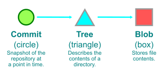
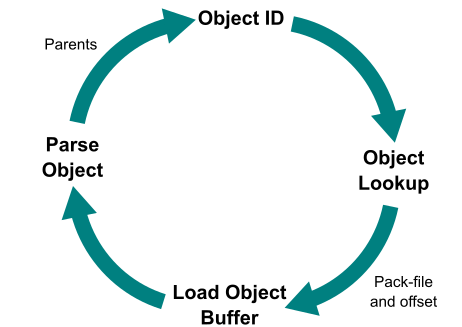
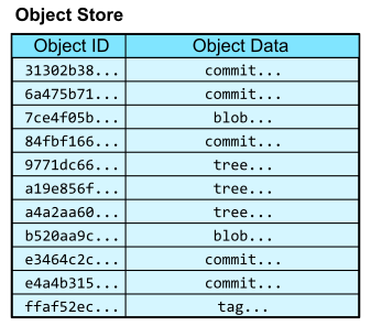
For a quick refresher on how we represent Git objects, see the key below.

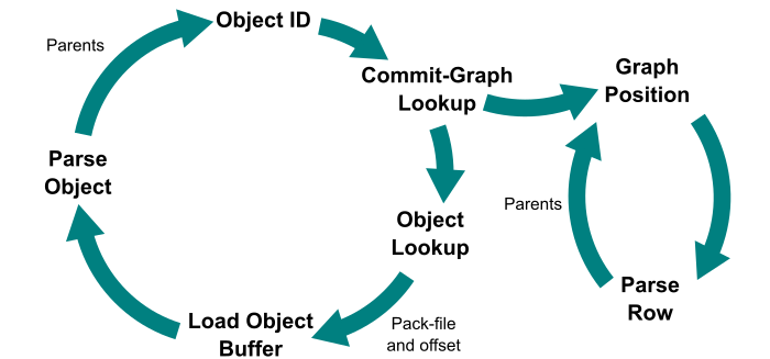
As discussed in part II, Git’s commit history can be stored in the commit-graph file for fast commit history queries. In this way, Git could walk all of the commits from the haves, then walk to their root trees, then recursively walk trees until finding all trees and blobs reachable from those commits. During this walk, Git can mark each object in-memory with a special flag indicating it is in this reachable set.
To find the reachable set difference, Git can walk from the want objects following each commit parent, root tree, and recursively through the trees. This second walk ignores the objects that were marked in the previous step so each visited object is part of the set difference.
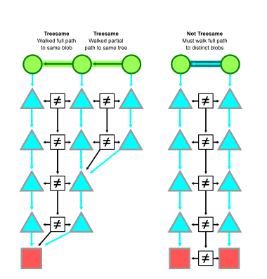
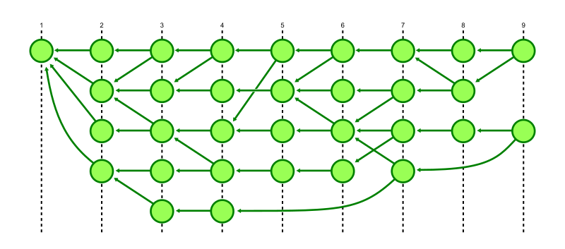
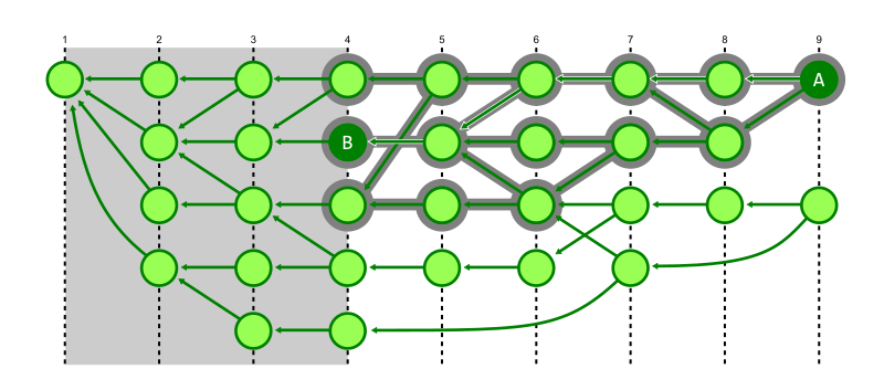
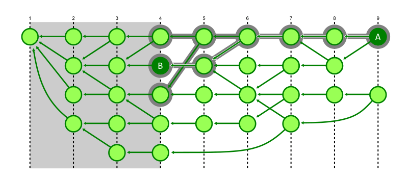
In the figure below, the commit B is a have and the commit A is a want. Two sets are shown. First, everything reachable from B is grouped into a set. The second set is the reachable set difference containing everything reachable from A but not reachable from B.

While this walking algorithm is a natural one to consider, it has a number of significant performance penalties.
First, we will spend a lot of time parsing trees in order to discover their tree entries. We noted in part III that tree parsing is expensive and that was when talking about file history where we only needed to parse trees along a single path. In addition, there are usually many tree entries that point to the same object. For example, an open source license file is usually added once and never modified in a repository. By contrast, almost every commit has a distinct root tree. Thus, each commit introduces a tree with a tree entry pointing to that license file. Git needs to test if the license file is already in the set each time it parses that tree entry. That’s a lot of work. We will revisit how to reduce the time spent parsing trees and following tree entries later, though it will require a new data structure.
The second performance penalty is that this walk requires visiting the entire commit history and likely walking a majority of the Git objects. That cost is paid even if the only objects in the reachable set difference is one commit that changes the README, resulting in a total of one commit, one tree, and one blob in the set difference. The fact that the cost does not scale with the expected output means that even frequent fetches will not reduce this cost.
Thankfully, there is a way to tweak this algorithm to reduce this second cost without needing any new data structures.
Discovering a frontier
If we think about the reachable set difference problem from the perspective of an arbitrary directed graph, then the full walk algorithm of the previous section is the best we can do. However, the Git object graph has additional structure, including different types of objects. Git uses the structure of the commit history to its advantage here, as well as some assumptions about how Git repositories are typically used.
If we think about Git repositories as storing source code, we can expect that code is mostly changed by creating new code. It is rare that we revert changes and reintroduce the exact copy of a code file that existed in the past. With that in mind, walking the full commit history to find every possible object that ever existed is unlikely to be helpful in determining the set of “new” objects.
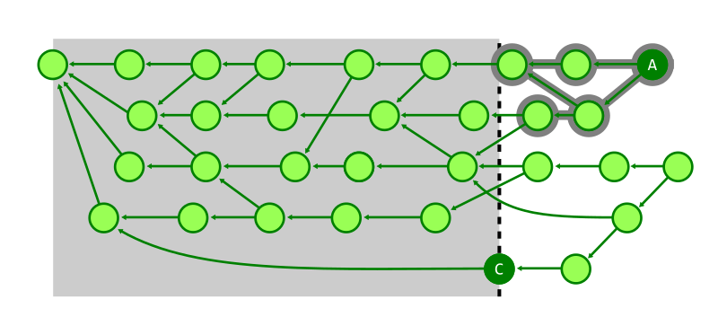
Instead of walking every object in the full commit history, Git uses the commit history of the haves and wants to discover a frontier of commits. These commits are the commits that are reachable from the haves but are on the boundary between the reachable set difference and the common history. For a commit A to be in the frontier, there must be at least one commit B whose parent is A and B is reachable from the wants but not reachable from the haves.
This idea of a frontier can be visualized using the git log --boundary query with a commit range parameter. In the example below, we are exploring the commits reachable from d02cc45c7a but not reachable from 3d8e3dc4fc. The commits marked with o are on this boundary.
$ git log --graph --oneline --boundary 3d8e3dc4fc..d02cc45c7a
*   acdb1e1053 Merge branch 'mt/checkout-count-fix'
|\
| * 611c7785e8 checkout: fix two bugs on the final count of updated entries
| * 11d14dee43 checkout: show bug about failed entries being included in final report
| * ed602c3f44 checkout: document bug where delayed checkout counts entries twice
* |   f0f9a033ed Merge branch 'cl/rerere-train-with-no-sign'
|\ \
| * | cc391fc886 contrib/rerere-train: avoid useless gpg sign in training
| o | bbea4dcf42 Git 2.37.1
|  /
o / 3d8e3dc4fc Merge branch 'ds/rebase-update-ref'
 /
o e4a4b31577 Git 2.37
Once Git has determined the commit frontier, it can simplify the object walk somewhat. Starting at the frontier, Git walks those root trees and then recursively all of the reachable trees. These objects are marked as reachable from the wants. Then, the second walk from the haves continues as normal, stopping when it sees objects in this smaller set.

With this new algorithm, we see that the cost of the object walk can be much smaller: we expect the algorithm to walk about as many objects as there exist from a few root trees, plus the new objects in the reachable set difference. This could still be a large set, but at least it does not visit every object in the full history. As part of this, we have many fewer repeated tree entries since they are rarely repeated within a walk from a few root trees.
There is an additional cost to this algorithm, though. We might increase the size of the resulting set! If some of the commits in the set difference really are reverts, then they could be “reintroducing” an older object into the resulting set. If this commit reverted the file at a given path, then every commit in the frontier must not have that version of the file at its root tree. This exact revert case is rare enough that these new objects do not account for a significant drawback, but it is worth mentioning.
We can still do better! In the case of a monorepo, that cost of walking all of the trees in the frontier can still be significant. Is there a way that we can compute a reachable set difference more quickly? Yes, but it requires new data structures!
Reachability bitmaps
When considering set arithmetic, such as set differences, a natural data structure to use is a bitmap. Bitmaps represent sets by associating every possible object with a position, and then using an array of bits over those positions to indicate if each object is in the set. Bitmaps are frequently used by application databases as a query index. A bitmap can store a precomputed set of rows in a table that satisfy some property, helping to speed up queries that request data in that set.
The figure below shows how the object graph from the previous figures is laid out so that every object is associated with a bit position. The bitmap at the top has a 1 in the positions corresponding to objects reachable from the commit A. The other positions have value 0 showing that A cannot reach that object.

Computing the set difference between two bitmaps requires iterating over the bit positions and reporting the positions that have a 1 in the first bitmap and a 0 in the second bitmap. This is identical to the logical operation of “A AND NOT B,” but applied to every bit position.
In this way, Git can represent the reachable sets using bitmaps and then perform the set difference. However, computing each bitmap is at least as expensive as walking all of the reachable objects. Further, as currently defined, bitmaps take at least one bit of memory per object in the repository, which can also become too expensive.
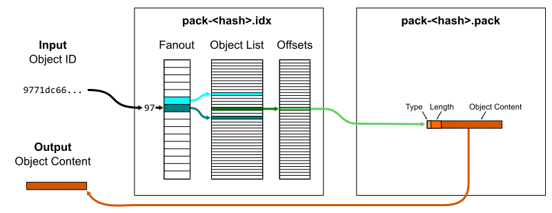
The critical thing that Git does to solve this cost of constructing the bitmaps is by precomputing the reachability bitmaps and storing them on disk. Recall from part I that Git uses compressed object storage files called packfiles to store the object contents. The git repack command takes all of the objects and creates a new packfile along with a pack-index.
The git repack --write-bitmap-index option computes reachability bitmaps at the same time as it repacks the Git object data into a new packfile. Each bit position is associated with an object in the packfile based on the order the objects appear in that packfile. In addition to the .pack and .idx files, a new .bitmap file stores these bitmaps. Git can also store reachability bitmaps across multiple packfiles using a multi-pack-index.
Each reachability bitmap is associated with a single Git commit. The bitmap stores the set of objects reachable from that commit. A .bitmap file can store reachability bitmaps corresponding to one or more commits.
If every commit had a reachability bitmap, then we could compute the reachable set difference from a set of haves and wants using the following process:
- Take the bitmap for each ‘have’ commit and merge them together into the union bitmap storing every object reachable from at least one ‘have’ commit.
- Take the bitmap for each ‘want’ commit and merge them together into the union bitmap storing every object reachable from at least one ‘want’ commit.
- Perform a set difference on the bitmaps created in the previous step.
The figure below shows this third step of performing the set difference on the two reachability bitmaps. The “A – B” bitmap is formed by including a 1 if and only if that position has a 1 in the A bitmap and a 0 in the B bitmap.

Unfortunately, computing and storing a reachability bitmap for every commit in the entire repository is not realistic. First, consider that each bitmap can take up one bit per object in the repository, then multiply that by the number of commits in the repository to get quadratic growth! This isn’t exactly a lower bound on the size of these bitmaps since Git uses a compressed bitmap encoding as well as a form of delta compression between bitmaps. However, the cost of computing and storing each bitmap is still significant.
Even if we were able to store a reachability bitmap for every commit, it is possible that a new commit is pushed to the repository and then is requested by a fetch before a reachability bitmap could be computed for it. Thus, Git needs some way to compute the reachable set difference even when the requested haves and wants do not have pre-computed bitmaps.
Git solves this by using a commit history walk. Starting at the haves, Git walks the commit history until finding a commit that has a precomputed reachability bitmap. That bitmap is used as a starting point, and the commit walk halts when it finds another reachability bitmap or finds a commit that is already contained in the reachable set because its bit is 1 in the bitmap. After the commit set is explored, Git walks the trees starting at the root trees, ignoring any trees that already exist in the reachability bitmap.
In this way, Git can dynamically compute the reachability bitmap containing the full set of objects reachable from the haves. The process is repeated with the wants. Then, the set difference is computed from those two bitmaps.
If the set of precomputed bitmaps is chosen carefully enough and the object order is selected in such a way that the bitmaps compress efficiently, these operations can be done while walking an incredibly small number of objects and using significantly less memory.
With proper maintenance of the reachability bitmap index, these reachable set difference queries can be much faster than the previous frontier walking strategy while also computing the exact set difference. The extra objects that could appear using the frontier algorithm do not appear using the precomputed bitmaps.
If you want to read more about how commits are chosen for bitmaps or how the bitmaps are compressed, read the original announcement of reachability bitmaps which goes into even greater detail. In particular, that post goes very deep on the fact that the object data is sent over the wire using the same packfile format as the on-disk representation discussed in part I, except that Git allows reference deltas to refer to objects already on the client’s machine. The fact that the on-disk representation and the network transfer format use this common format is one of Git’s strengths.
Pushing to a remote
The previous algorithms were focused on computing the reachable set difference required during a git fetch command. After the client sends the list of haves and wants, the server computes the set difference and uses that to send the objects to the client. The natural opposite of this operation is the git push command where the client sends new objects to the server.
We could use the existing algorithm, but we need to flip around some meanings. The haves and wants become commits that “the server has” and “the client wants the server to have”. One caveat is that, by default, git push doesn’t do a negotiation at the start and instead thinks about the references in refs/remotes/<remote> as the set of haves. You can enable the push.negotiate config option if you find this negotiation to be valuable. This negotiation is important if you have not updated your refs/remotes/<remote> references through a git fetch in a while. The negotiation is more useful if you are using background maintenance because you are more likely to have most of the objects the remote will advertise in the negotiation.
Other than reversing the roles of the haves and wants, the goals of git push are exactly the same as git fetch. The command synchronizes objects from one repository to another. However, we can again think about the typical use of the commands to see that there are some asymmetries.
When a client runs git fetch, that command will typically download new objects from several other contributors to that repository, perhaps merged together by pull requests. These changes are likely to include changes to many files across several directories. When a client runs git push, the information that is new to the remote is typically a single topic branch created by a single contributor. The files modified by this effort are likely to be smaller in number than the git fetch case.
Git exploits this asymmetry using a custom reachable set difference algorithm tailored to these expectations.
Sparse reachable set difference
One major asymmetry with git push is that clients rarely find it worth the cost to precompute reachability bitmaps. That maintenance cost is too CPU intensive compared to the number of times git push is run by a typical user. For Git servers, reachability bitmaps are absolutely critical to efficient function, so that extra maintenance is easy to justify.
Without reachability bitmaps, Git falls back to the frontier algorithm when computing the reachable set difference. This works mostly fine for small projects, but when the client repository is very large, the cost of walking every object reachable from even a single root tree becomes too expensive.
This motivated the sparse reachable set difference algorithm. This algorithm is enabled by the pack.useSparse config option, which is now enabled by default. In addition to using the commit history to construct a frontier of commits, the sparse algorithm uses the structure of the trees themselves to compute the reachable set difference.
Just like the frontier algorithm, Git computes the commit frontier as a base of which objects are in common between the haves and wants. Then, instead of walking all the trees reachable from the root trees in the frontier and then walking the root trees from the wants, Git walks these trees in a single walk.
Instead of exploring the object graph directly by walking from tree to tree one at a time, Git changes the walk to do a breadth-first search on the paths available in these trees. Each node of this walk consists of a path and a set of trees. Each tree is marked as uninteresting or interesting, depending on whether they come from the commit frontier or not, respectively.
The walk is initialized with the empty path and the set of root trees from our commit frontier and the commits reachable from the wants. As Git explores a node, it iterates over each tree in the associated set. For each of those trees, it parses the tree entries and considers the path component from each. If the entry points to a blob, then those blobs are marked as interesting or uninteresting. If the entry points to a tree, then the path component leads to a new node and that tree is added to that node’s tree set.
During this walk, uninteresting trees mark their child trees as uninteresting. When visiting a node, Git skips the node if every contained tree is uninteresting.
These “all uninteresting” nodes represent directories where there are no new objects in the reference being pushed relative to the commit frontier. For a large repository and most changes, the vast majority of trees fit in this category. In this way, this sparse algorithm walks only the trees that are necessary to discover these new objects.

This sparse algorithm is discussed in more detail in the blog post announcing the option when it was available in Git 2.21.0, though the pack.useSparse option was enabled by default starting in Git 2.27.0.
Heuristics and query planning
In this blog series, we are exploring Git’s internals as if they were a database. This goes both directions: we can apply database concepts such as query indexes to frame these advanced Git features, but we can also think about database features that do not have counterparts in Git.
This area of synchronization is absolutely one area where database concepts could apply, but currently do not. The concept I’m talking about is query planning.
When an application database is satisfying a query, it looks at the query and the available query indexes, then constructs a plan for executing the query. Most query languages are declarative in that they define what output they want, but not how to do that operation. This gives the database engine flexibility in how to best use the given information to satisfy the query.
When Git is satisfying a reachable set difference query, it does the most basic level of query planning. It considers its available query indexes and makes a choice on which to use:
- If reachability bitmaps exist, then use the bitmap algorithm.
- Otherwise, if
pack.useSparseis enabled, then use the sparse algorithm. - If neither previous case holds, then use the frontier algorithm.
This is a simple, and possibly unsatisfying way to do query planning. It takes the available indexes into account, but does not check how well those indexes match with the input data.
What if the reachability bitmaps are stale? We might spend more time in the dynamic bitmap computation than we would in the frontier algorithm.
We can walk commits really quickly with the commit-graph. What if there are only a few commits reachable from the wants but not reachable from the frontier? The sparse algorithm might be more efficient than using reachability bitmaps.
This is an area where we could perform some experiments and create a new, dynamic query planning strategy that chooses the best algorithm based on some heuristics and the shape of the commit history.
Already there is some ability to customize this yourself. You can choose to precompute reachability bitmaps or not. You can modify pack.useSparse to opt out of the sparse algorithm.
A change was merged into the Git project that creates a push.useBitmaps config option so you can compute reachability bitmaps locally but also opt out of using them during git push. Reachability bitmaps are integrated with other parts of Git, so it can be helpful to have them around. However, due to the asymmetry of git fetch and git push, the sparse algorithm can still be faster than the bitmap algorithm. Thus, this config will allow you to have the benefits of precomputed reachability bitmaps while also having fast git push commands. Look forward to this config value being available soon in Git 2.38.0!
Come back tomorrow for the final installment!
Now that we’ve explored all of the different ways Git operates on a repository, we have a better grasp on how Git scales its algorithms with the size of the repository. When application databases grow too quickly, many groups resort to sharding their database. In the next (and final!) part of this blog series, we will consider the different ways to scale a Git repository, including by sharding it into smaller components.
I’ll also be speaking at Git Merge 2022 covering all five parts of this blog series, so I look forward to seeing you there!
![[Security Nation] Gordon “Fyodor” Lyon on Nmap, the Open-Source Security Scanner](https://blog.rapid7.com/content/images/2022/08/urbaneparty-blackhat-500px.jpg)