Post Syndicated from James Beswick original https://aws.amazon.com/blogs/compute/capturing-client-events-using-amazon-api-gateway-and-amazon-eventbridge/
This post is written by Tim Bruce, Senior Solutions Architect, DevAx.
Event producers are one of the three main components in an event-driven architecture. Event producers create and publish events to event routers, which send them to event consumers. Any portion of a system, including a mobile or web client, can be an event producer.
To extend the event model to your mobile and web clients, you must implement standards for security, messaging formats, and event storage.
This post shows how to build a client-enabled event-handling solution. It uses Amazon EventBridge, Amazon API Gateway, AWS Lambda, and Amazon Cognito. This architecture supports routing client events to internal and external destinations. It provides a blueprint that you can use to simplify the integration.
Overview
This example creates a RESTful API using API Gateway. It sends events directly to EventBridge without the need for compute services. In production, you have more requirements than only receiving and forwarding events. Additional requirements include security, user identification, validation, enrichment, transformation, event forwarding, and storing.
In this example, API Gateway provides security and user identification by invoking a Lambda authorizer. The authorizer generates a policy and returns client identification to API Gateway. API Gateway then performs request validation and message enrichment before forwarding the events to EventBridge.
EventBridge evaluates the events against rules and forwards the events to targets. The rules apply transformation to the events and forward an event to up to five targets. Targets include AWS services, such as Amazon Kinesis Data Firehose, and many third-party solutions, such as Zendesk, with HTTPS endpoints.
Lastly, Kinesis Data Firehose provides a cost-effective solution to store events into an Amazon S3 bucket. Before storing the events, Kinesis Data Firehose transforms records via Lambda transformers. It also partitions records using data in the record or calculated data via a Lambda function. Kinesis Data Firehose uses this partitioning data to create keys in the bucket and store matching records within the keys.
Example architecture

The example consists of the following resources defined in the AWS SAM template:
- An API Gateway instance to receive the messages.
- A Lambda authorizer to validate requests.
- An EventBridge event bus to receive events.
- An EventBridge rule to forward all events to Kinesis Data Firehose.
- An EventBridge rule to forward specific events to Zendesk.
- An EventBridge API destination to connect to your Zendesk.
- A Kinesis Data Firehose to transform, partition, and store events in an S3 bucket.
- A Lambda Kinesis Data Firehose data transformation.
- An S3 bucket to store event data.
Data flow

- Application clients collect or generate the events.
- The client sends the events to API Gateway as URL-encoded JSON. The client includes the user’s JWT in an authorization header with the request for validation.
- The Lambda authorizer validates the JWT with Amazon Cognito and returns the user’s unique clientID value to API Gateway.
- API Gateway transforms the request into events, appending clientId, the bus name, and environment.
- API Gateway sends the events to EventBridge.
- EventBridge rules match the events and:
- Forwards all client events to Kinesis Data Firehose.
- Forwards client events with detail.eventType of “loyaltypurchase” to Zendesk.
- Kinesis Data Firehose receives the records.
- The Kinesis Data Firehose data transformation processes each record, moving the client ID to the detail object.
- Kinesis Data Firehose partitions the records and stores them in an S3 bucket.
Overall design
The following sections discuss details of the solution, starting from the event in a web or mobile client. This solution requires the client to create an HTTPS request, including the user’s JWT as an authorization header.
{"entries": [{"entry": "{\"eventType\": \"searching\", \"schemaVersion\":1, \"data\": {\"searchTerm\":\"games\"}}"}]}
The preceding JSON shows a sample request body for this solution. The top-level item “entries” is an array of “entry” items. API Gateway will translate each “entry” to the event-detail field in EventBridge events. The client must escape the data for “entry” to prevent translation errors.
API Gateway and Lambda authorizer
API Gateway receives the request and validates the JWT by invoking the Lambda authorizer. The authorizer generates a policy allowing the request for valid tokens. It adds the Amazon Cognito “custom:clientId” custom attribute to the response context before returning the response to API Gateway. The “custom:clientId” attribute is a unique client identifier in the form of a UUID that downstream systems can use to retrieve data about the customer.
API Gateway validates the request by matching the request body against a model. Models represent what a request should look like. A mapping template then transforms valid requests to the format required by EventBridge. Mapping templates use velocity templating language (VTL) to do this.

This mapping template uses a #foreach loop to process the array “entries” from the request body. The process enriches each event with the user’s “custom:clientId” and stage variables for bus name and environment from API Gateway.

The preceding API Gateway AWS integration enables API Gateway to send the events to EventBridge without using compute services, such as Lambda or Amazon EC2. The integration and IAM execution role enable API Gateway to call the EventBridge PutEvents API to do this.
EventBridge rules and transformations
EventBridge rules match events against criteria, transform the events, and forward the events to targets. There are two rules in this example. One processes events for Zendesk tickets and the other forwards data to Kinesis Data Firehose to store events for triage and analytics.
This example creates service tickets in the Zendesk ticketing system. The tickets trigger agents to contact customers who are expecting a call to complete their purchases. The software client, by sending the event directly, reducing time-to-action for back-office processes and helping improve customer satisfaction.

This rule matches client event messages for loyalty purchases and forwards details to the Zendesk API. The rule includes a transformation, which selects a portion of the event before sending the information to the target.
EventBridge uses an API destination to store details about the HTTP endpoint and usage policies. Additionally, an EventBridge connection and an AWS Secrets Manager secret store details. These include the authentication policy and authentication credentials to connect to the API destination.

Successfully processed events open tickets in Zendesk using the API destination. Agents now have a list of customers to contact.
Enterprises often require storing the events for troubleshooting or analytics. EventBridge does not include a newline between records when forwarding events to Kinesis Data Firehose. Because of this, it may be more challenging to discern each record when analyzing the data.
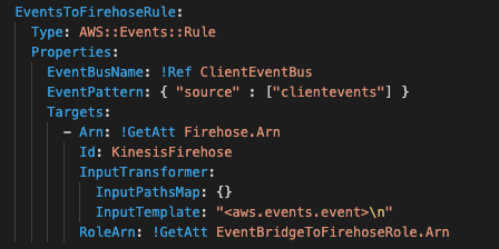
A rule for all client events changes this behavior. This AWS CloudFormation snippet defines the rule that will transform each event, adding a new line after each. The “\n” character in the InputTemplate field adds the separator between records before forwarding the data to Kinesis Data Firehose.
After, Kinesis Data Firehose receives each record separated by a new line, enabling both triage and analytics without extra overhead.
Kinesis Data Firehose to S3
Kinesis Data Firehose is a cost-effective way to batch and write records to S3. It offers optional transformation capabilities by invoking a Lambda function. This example uses a Lambda function that moves the “clientID” field to the detail section of the event record.
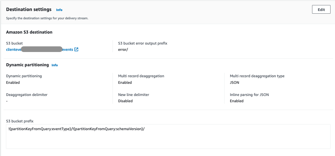
Kinesis Data Firehose also supports dynamic partitioning of records when writing to S3. It selects data from the records or data calculated by a Lambda function. In this example, it selects data from the records to store data in separate folders in S3.
Event durability considerations
You can extend this example using an EventBridge archive and Amazon Kinesis Data Streams. Archiving allows you to create an encrypted archive of matching events. You can define the data retention in days, from one through indefinite. You can replay events from your archive when you must re-process data.
Kinesis Data Streams is a serverless data streaming solution. The EventBridge rule for all records can forward data to Kinesis Data Streams instead of Kinesis Data Firehose. Multiple applications can consume the Kinesis Data Streams. Kinesis Data Firehose would consume this stream of data and store it in S3.
Prerequisites
You need the following prerequisites to deploy the example solution:
- AWS account
- AWS CLI
- AWS Serverless Application Model (AWS SAM) CLI
- Python 3.9
- An AWS Identity and Access Management (IAM) role with appropriate access.
- A Zendesk trial account
- A Zendesk API key
Implementation
The full source of the solution is in the GitHub repository and is deployed with AWS SAM.
- Create a Secrets Manager secret using the command the AWS CLI:
aws secretsmanager create-secret --name proto/Zendesk --secret-string '{"username":"<YOUR EMAIL>","apiKey":"<YOUR APIKEY>"} - Clone the solution repository using git:
git clone https://github.com/aws-samples/client-event-sample - Build the AWS SAM project:
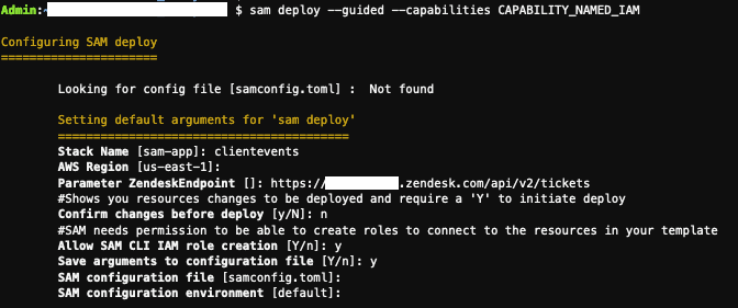
sam build --use-container - Deploy the project using AWS SAM:
sam deploy --guided --capabilities CAPABILITY_NAMED_IAM
- From the outputs from the deployment, set the following shell variables:
APPCLIENTID=<output APPCLIENTID> APIID=<output APIID> REGION=<region you deployed to> - Create a user in Amazon Cognito using the AWS CLI:
aws cognito-idp sign-up --client-id $APPCLIENTID --username <YOUR USER ID> --password <YOUR PASSWORD> --user-attributes Name=email,Value=<YOUR EMAIL> - After you receive the confirmation code, confirm the user using the AWS CLI:
aws cognito-idp confirm-sign-up --client-id $APPCLIENTID --username <userid> --confirmation-code <confirmation code> - Test the user login with the AWS CLI:
aws cognito-idp initiate-auth --auth-flow USER_PASSWORD_AUTH --client-id $APPCLIENTID --auth-parameters USERNAME=<YOUR USER ID>,PASSWORD=<YOUR PASSWORD>
If successful, this returns a JSON web token (JWT).
Testing the client event solution
- The sample repository includes an event generator in the util directory. The generator uses your credentials and simulates events from a user’s software client. From the utils directory, run the generator:
python3 generator.py
 --minutes <minutes to run generator> --batch <batch size from 1-10>
 --errors <True|False> --userid <YOUR USER ID> --password <YOUR
PASSWORD> --region $REGION --appclientid $APPCLIENTID --apiid $APIID - Log in to your Zendesk console and view the created tickets.
- After five minutes, review the “clientevents” bucket to view the event records.
Cleaning up
To remove the example:
- Delete the data stored in the clientevents buckets created from the template.
- Delete the stack using the command:
sam delete --stack-name clientevents - Delete the secret using the command:
aws secretsmanager delete-secret --secret-id <arn of secret>
Conclusion
This post shows how to send client events to an API and EventBridge to enable new customer experiences. The example covers enabling new experiences by creating a way for software clients to send events with minimal custom code. This blueprint shows how you can include client events in your solution, featuring validation, enrichment, transformation, and storage.
You can modify the example code provided here for your use in your organization. This enables your client software to register events without modifying backend code.
For more serverless learning resources, visit Serverless Land.