Tag Archives: serverless

AWS Lambda enhances event processing with provisioned mode for SQS event-source mapping

Post Syndicated from Micah Walter original https://aws.amazon.com/blogs/aws/aws-lambda-enhances-sqs-processing-with-new-provisioned-mode-3x-faster-scaling-16x-higher-capacity/

Today, we’re announcing the general availability of provisioned mode for AWS Lambda with Amazon Simple Queue Service (Amazon SQS) Event Source Mapping (ESM), a new feature that customers can use to optimize the throughput of their event-driven applications by configuring dedicated polling resources. Using this new capability, which provides 3x faster scaling, and 16x higher concurrency, you can process events with lower latency, handle sudden traffic spikes more effectively, and maintain precise control over your event processing resources.

Modern applications increasingly rely on event-driven architectures where services communicate through events and messages. Amazon SQS is commonly used as an event source for Lambda functions, so developers can build loosely coupled, scalable applications. Although the SQS ESM automatically handles queue polling and function invocation, customers with stringent performance requirements have asked for more control over the polling behavior to handle spiky traffic patterns and maintain low processing latency.

Provisioned mode for SQS ESM addresses these needs by introducing event pollers, which are dedicated resources that remain ready to handle expected traffic patterns. These event pollers can auto scale up to 1000 per concurrent executions per minute, more than three times faster than before to handle sudden spikes in event traffic and provide up to 20,000 concurrency–16 times higher capacity to process millions of events with Lambda functions. This enhanced scaling behavior helps customers maintain predictable low latency even during traffic surges.

Enterprises across various industries, from financial services to gaming companies, are using AWS Lambda with Amazon SQS to process real-time events for their mission-critical applications. These organizations, which include some of the largest online gaming platforms and financial institutions, require consistent subsecond processing times for their event-driven workloads, particularly during periods of peak usage. Provisioned mode for SQS ESM is a capability you can use to meet your stringent performance requirements while maintaining cost controls.

Enhanced control and performance

With provisioned mode, you can configure both minimum and maximum numbers of event pollers for your SQS ESM. Each event poller represents a unit of compute that handles queue polling, event batching, and filtering before invoking Lambda functions. Each event poller can handle up to 1 MB/sec of throughput, up to 10 concurrent invokes, or up to 10 SQS polling API calls per second. By setting a minimum number of event pollers, you enable your application to maintain a baseline processing capacity that can immediately handle sudden traffic increases. We recommend that you set the minimum event pollers required to handle your known peak workload requirements. The optional maximum setting helps prevent overloading downstream systems by limiting the total processing throughput.

The new mode delivers significant improvements in how your event-driven applications handle varying workloads. When traffic increases, your ESM detects the growing backlog within seconds and dynamically scales event pollers between your configured minimum and maximum values three times faster than before. This enhanced scaling capability is complemented by a substantial increase in processing capacity, with support for up to 2 GBps of aggregate traffic, and up to 20K concurrent requests—16x higher than previously possible. By maintaining a minimum number of ready-to-use event pollers, your application achieves predictable performance, handling sudden traffic spikes without the delay typically associated with scaling up resources. During low traffic periods, your ESM automatically scales down to your configured minimum number of event pollers, which means you can optimize costs while maintaining responsiveness.

Let’s try it out

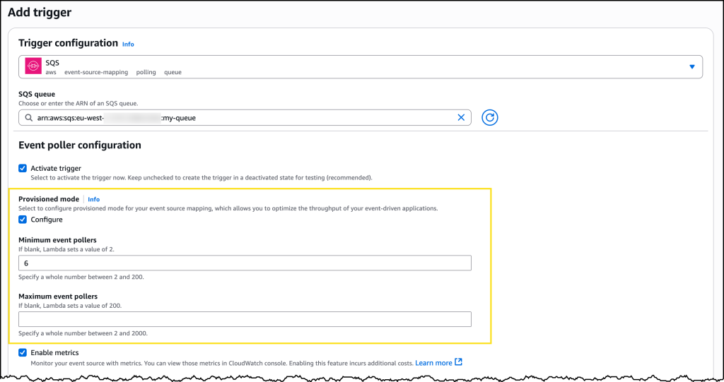
Enabling provisioned mode is straightforward in the AWS Management Console. You need to already have an SQS queue configured and a Lambda function. To get started, in the Configuration tab for your Lambda function, choose Triggers, then Add trigger. This will bring up a user interface where you can configure your trigger. Choose SQS from the dropdown menu for source and then select the SQS queue you want to use.

Under Event poller configuration, you will now see a new option called Provisioned mode. Select Configure to reveal settings for Minimum event pollers and Maximum event pollers, each with defaults and minimum and maximum values displayed.

Configuration panel for SQS provisioned Mode

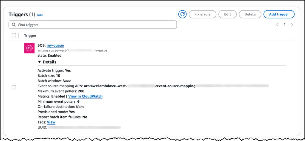
After you have configured Provisioned mode, you can save your trigger. If you need to make changes later, you can find the current configuration under the Triggers tab in the AWS Lambda configuration section, and you can modify your current settings there.

SQS Provisioned Poller confiig

Monitoring and observability

You can monitor your provisioned mode usage through Amazon CloudWatch metrics. The ProvisionedPollers metric shows the number of active event pollers processing events in one-minute windows.

Now available

Provisioned mode for Lambda SQS ESM is available today in all commercial AWS Regions. You can start using this feature through the AWS Management Console, AWS Command Line Interface (AWS CLI), or AWS SDKs. Pricing is based on the number of event pollers provisioned and the duration they’re provisioned for, measured in Event Poller Units (EPUs). Each EPU supports up to 1 MB per second throughput capacity per event poller, with minimum 2 event pollers per ESM. See the AWS pricing page for more information on EPU charges.

To learn more about provisioned mode for SQS ESM, visit the AWS Lambda documentation. Start building more responsive event-driven applications today with enhanced control over your event processing resources.

AWS Lambda networking over IPv6

Post Syndicated from John Lee original https://aws.amazon.com/blogs/compute/aws-lambda-networking-over-ipv6/

IPv4 address exhaustion is a challenge in modern networking, as most IPv4 addresses have been depleted with the growth of the internet. Previously, AWS Lambda only supported inbound and outbound connectivity over IPv4, but it has since introduced support for dual-stack endpoints, so that you can transition from IPv4 to IPv6. AWS continues to add support for IPv6, recently announcing support for inbound IPv6 connectivity over AWS PrivateLink, and dual-stack endpoint support for Amazon API Gateway.

With these IPv6 capabilities now available in Lambda, you should understand how to use them effectively. This post examines the benefits of transitioning Lambda functions to IPv6, provides practical guidance for implementing dual-stack support in your Lambda environment, and considerations for maintaining compatibility with existing systems during migration.

Benefits of transitioning

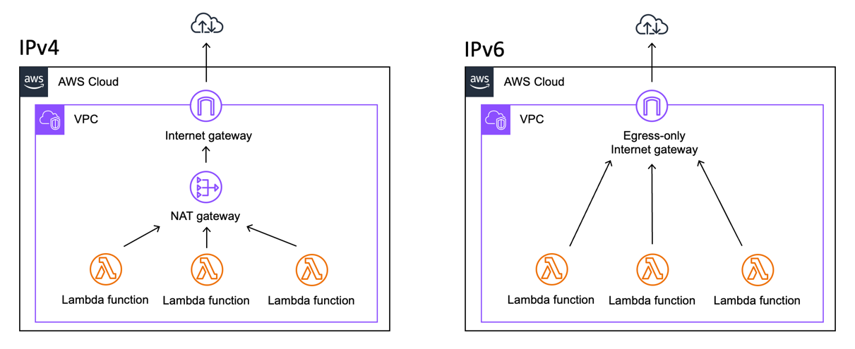
You can transition to IPv6 to future-proof your overall architecture by preparing ahead of the broader transition to IPv6, and establish compatibility with IPv6 clients or services. IPv6 also eliminates the need for a NAT gateway when the Lambda functions need internet connectivity from a private subnet in your Amazon Virtual Private Cloud (Amazon VPC). Lambda functions can direct traffic to the egress-only internet gateway, potentially eliminating the NAT gateway and its associated charges and streamlining network design. This transition provides cost savings, as egress-only internet gateways are free to use, as opposed to NAT gateways that incurs an hourly charge. Furthermore, IPv6 offers improved network efficiency by eliminating NAT translation overhead, so that Lambda functions can establish direct connections with clients. IPv6 also has more advantages such as native Quality of Service (QoS), which streamlines header structure and reduces packet fragmentations.

Architectural implications

Lambda functions are often deployed inside of a VPC to access VPC resources. For VPC Lambda functions to access the internet, routing traffic through an NAT gateway is a common approach. For Lambda functions with IPv6 support, Lambda functions can now route traffic directly through the egress-only internet gateway, which eliminates the need for a NAT gateway and the extra hop, as shown in the following figures.

architecture diagram showing egress traffic in both ipv4 and ipv6 environments

Figure 1. Lambda internet connectivity through a NAT Gateway (IPv4) and Lambda internet connectivity through an egress-only internet gateway (IPv6).

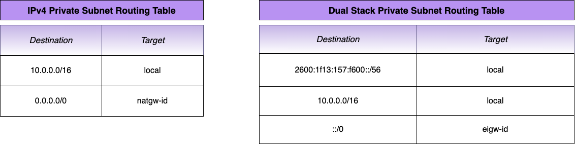
Once the egress-only internet gateway is in place, you need to update the route table to reflect this. If you have used 0.0.0.0/0 as the default route for IPv4 traffic, you should add ::/0 as the default route for IPv6 traffic. The following image shows the updated route table.

ipv4 and ipv6 route tables

Figure 2. Lambda private subnet routing tables for an NAT Gateway (IPv4) as opposed to a dual-stack including an egress-only internet gateway (IPv6)

If you are using Lambda function URLs, no transition is needed. Lambda function URLs are inherently IPv6-capable and can be accessed by IPv6 clients without needing architectural changes or modifications. This IPv6 compatibility for function URLs operates independently of your Lambda function’s VPC configuration, and clients can reach your Lambda function URLs over IPv6 even when dual-stack is not enabled in your VPC.

For Lambda functions that interact exclusively with AWS services through internal traffic, IPv6 offers limited benefits. For example, in an architecture where a Lambda function processes requests from Amazon API Gateway and queries a database hosted on Amazon Relational Database Service (Amazon RDS), no architectural change is expected. Internal traffic routes using the RDS cluster endpoint and Lambda Amazon Resource Name (ARN), not IP addresses, as shown in the following figure.

architecture diagram showing traffic going through API GW, Lambda, and RDS

Figure 3. A common architecture pattern where Lambda processes events from API Gateway and reads/writes to Amazon RDS. You reference the Lambda function ARN and RDS cluster endpoint instead of IPv4/IPv6 addresses.

Transitioning from IPv4 to IPv6

By default, Lambda functions communicate over IPv4 to their destinations. For Lambda functions to communicate with IPv6 destinations, dual-stack VPC configuration is needed. This allows Lambda functions to communicate over both IPv4 and IPv6.

If your VPC does not have IPv6 support, then you need to first add IPv6 support for your VPC. You need to follow these steps to enable IPv6 traffic for a Lambda function:

  1. Assign IPv6 block to VPC: You need to edit the existing VPC CIDRs to add an IPv6 CIDR block. If you select the option of Amazon-provided IPv6 CIDR block, then you are assigned a /56 IPv6 CIDR block from the Amazon pool of IPv6 addresses. You also have the option to assign an Amazon VPC IP Address Manager allocated or your own IPv6 CIDR block.
  2. Assign IPv6 block to Subnets: After assigning an IPv6 CIDR block to the VPC, you must manually configure IPv6 CIDR blocks for each existing subnet, with each subnet receiving a portion of the VPC’s IPv6 address space.
  3. Update route tables: For your Lambda function’s IPv6 traffic to reach the internet, you need to add a route (::/0) to the egress-only internet gateway.
  4. Update security groups: By default, security groups allow all outbound traffic. To restrict outbound IPv6 traffic from your Lambda function, you must remove the default egress rule and add specific restrictive outbound rules. For inbound traffic, security group rules are needed when your Lambda function receives direct network connections, such as traffic through AWS PrivateLink connections.
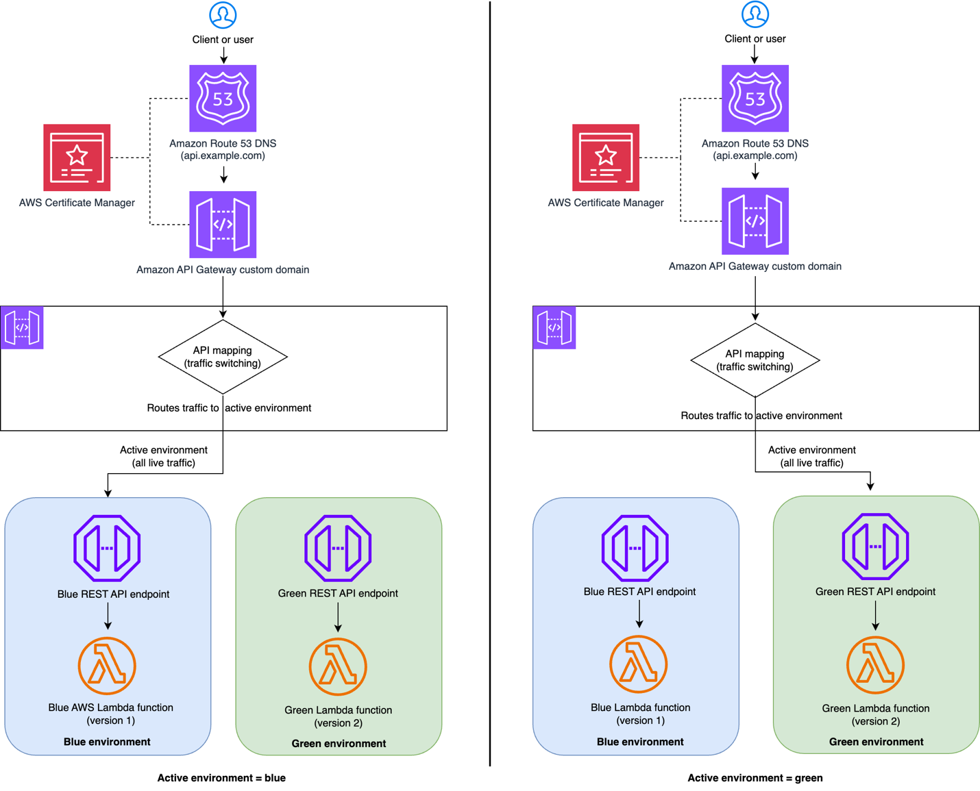
  5. Enable IPv6 dual-stack on the Lambda function: When you assign IPv6 addresses for your Lambda function’s subnet, you can enable IPv6 dual-stack for the Lambda function. Then, Lambda creates new Elastic network interfaces (ENI) with IPv4 and IPv6 protocols with both IPv4 and IPv6 addresses. Although most updates to the Lambda function have zero downtime, enabling dual-stack may cause disruption in connectivity. To prevent downtime during the transition, we recommend using Lambda versions and aliases to implement a blue/green deployment strategy. You can publish your IPv6-enabled Lambda function as a new version while keeping the current version active and serve traffic through the alias. After testing the new IPv6 version, you can update the alias to switch the traffic. This approach provides a rollback capability, and you can revert the alias to point back to the previous version if needed.

When you have completed these steps, your Lambda function can support dual-stack networking and communicate over both IPv4 and IPv6.

Conclusion

In this post, we covered the benefits of transitioning your AWS Lambda functions from IPv4 to IPv6, the architectural implications, and steps for how you could make the transition.We recommend transitioning your Lambda functions to support both IPv4 and IPv6 traffic to gain its benefits. The Lambda IPv6 support helps address IPv4 exhaustion while providing cost savings and network clarification. Once organizations transition to supporting only IPv6 traffic, they can eliminate NAT gateways for Lambda functions needing internet access, thus reducing both costs and architectural complexity. As AWS expands IPv6 support across services, transitioning Lambda functions to dual-stack networking positions organizations for long-term compatibility while delivering immediate operational benefits.

For more information on how to enable IPv6 access for Lambda functions in dual-stack VPC, see the Lambda documentation. For more serverless learning resources, visit Serverless Land.

Optimizing nested JSON array processing using AWS Step Functions Distributed Map

Post Syndicated from Biswanath Mukherjee original https://aws.amazon.com/blogs/compute/optimizing-nested-json-array-processing-using-aws-step-functions-distributed-map/

When you’re working with large datasets, you’ve likely encountered the challenge of processing complex JSON structures in your automated workflows. You need to preprocess arrays within nested JSON objects before you can run parallel processing on them. Extracting data used to require custom code and extra processing steps, delaying you from building your core application logic.

With AWS Step Functions Distributed Map, you can process large datasets with concurrent iterations of workflow steps across data entries. Using the enhanced ItemsPointer feature of Distributed Maps, you can extract array data directly from JSON objects stored in Amazon S3. Alternatively, for JSON object as state input, you can use Items (JSONata) or ItemsPath (JSONPath). With this enhancement you can point directly to arrays nested within JSON structures, eliminating the need for custom preprocessing of your data. With ItemsPointer, Items, and ItemsPath you can select the nested array data and simplify your workflows.

In this post, we explore how to optimize processing array data embedded within complex JSON structures using AWS Step Functions Distributed Map. You’ll learn how to use ItemsPointer to reduce the complexity of your state machine definitions, create more flexible workflow designs, and streamline your data processing pipelines—all without writing additional transformation code or AWS Lambda functions.

This post is part of a series of post about AWS Step Functions Distributed Map:

Use case: e-commerce product data enrichment

In this e-commerce use case example, you’ll build a sample application that demonstrates processing of product inventory data for an e-commerce application using AWS Step Functions Distributed Map. The application receives a JSON file from an upstream application containing an array of product information. The Step Functions workflow reads the JSON file containing product data from an S3 bucket and iterates over the array to enrich each product data in the array.

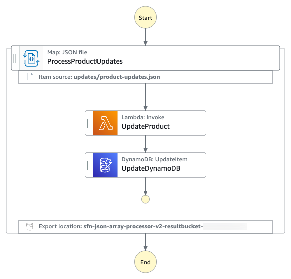
The following diagram presents the AWS Step Functions state machine.

JSON array processing workflow

JSON array processing workflow

The JSON array is processed using the following workflow:

  1. The state machine reads the product-updates.json file from an input S3 bucket. The file contains a JSON array of products.
  2. The Distributed Map state in the state machine, selects the JSON array node using ItemsPointer and iterates over the JSON array.
  3. For each of the items within the array, the state machine invokes a Lambda function for data enrichment. The Lambda function adds product stock and price information to the product data.
  4. The state machine saves the updated product data in an Amazon DynamoDB table.
  5. Finally, the state machine uploads the execution metadata into an output S3 bucket. See limits related to state machine executions and task executions.

MaxConcurrency can be configured to specify the number of child workflow executions in a Distributed Map that can run in parallel. If not specified, then Step Functions doesn’t limit concurrency and runs 10,000 parallel child workflow executions.

You can read a JSON file from a S3 bucket using ItemReader and its sub-fields. If the JSON file, from the S3 bucket, contains a nested object structure, you can select the specific node with your data set with an ItemsPointer. For example, the following input JSON file:

{
  "version": "2024.1",
  "timestamp": "2025-09-26T10:49:36.646197",
  "productUpdates": {
    "items": [
      {
        "productId": "PROD-001",
        "name": "Wireless Headphones",
        "price": 79.99,
        "stock": 150,
        "category": "Electronics"
      },
      {
        "productId": "PROD-002",
        "name": "Smart Watch",
        "category": "Electronics"
      },
      …
    ]
  }
}

The following JSONata-based workflow configuration extracts a nested list of products from productUpdates/items:

"ItemReader": {
   "Resource": "arn:aws:states:::s3:getObject",
   "ReaderConfig": {
      "InputType": "JSON",
      "ItemsPointer": "/productUpdates/items"
   },
   "Arguments": {
      "Bucket": "amzn-s3-demo-bucket",
      "Key": "updates/product-updates.json"
   }
}

For JSONPath-based workflow note that Arguments is replaced with Parameters:

"ItemReader": {
   "Resource": "arn:aws:states:::s3:getObject",
   "ReaderConfig": {
      "InputType": "JSON",
      "ItemsPointer": "/productUpdates/items"
   },
   "Arguments": {
      "Bucket": "amzn-s3-demo-bucket",
      "Key": "updates/product-updates.json"
   }
}

The ItemReader field is not needed when your dataset is JSON data from a previous step. ItemsPointer is only applicable when the input JSON objects read from an S3 bucket. If you are using JSON as state input to a Distributed Map, then you can use the ItemsPath (for JSONPath) or Items (for JSONata) field to specify a location in the input that points to JSON array or object used for iterations.

Prerequisite

To use Step Functions Distributed Map, verify you have:

Set up and run the workflow

Run the following steps to deploy the Step Functions state machine.

  1. Clone the GitHub repository in a new folder and navigate to the project folder.
    git clone https://github.com/aws-samples/sample-stepfunctions-json-array-processor.git
    cd sample-stepfunctions-json-array-processor

  2. Run the following commands to deploy the application.
    sam deploy --guided

    Enter the following details:

    • Stack name: Stack name for CloudFormation (for example, stepfunctions-json-array-processor)
    • AWS Region: A supported AWS Region (for example, us-east-1)
    • Accept all other default values.

    The outputs from the sam deploy will be used in the subsequent steps.

  3. Run the following command to generate product-updates.json file containing a nested JSON array of sample products and upload the product-updates.json file to the input S3 bucket. Replace InputBucketName with the value from sam deploy output.
    python3 scripts/generate_sample_data.py <InputBucketName>

  4. Run the following command to start execution of the Step Functions workflow. Replace the StateMachineArn with the value from sam deploy output.
    aws stepfunctions start-execution \
      --state-machine-arn <StateMachineArn> \
      --input '{}'

    The state machine reads the input product-updates.json file and invokes a Lambda function to update the database for every product in the array after adding price and stock information. The execution metadata is also uploaded into the results bucket.

Monitor and verify results

Run the following steps to monitor and verify the test results.

  1. Run the following command to get the details of the execution. Replace executionArn with your state machine ARN.
    aws stepfunctions describe-execution --execution-arn <executionArn>

    Wait until the status shows SUCCEEDED.

  2. Run the following commands to validate the processed output from ProductCatalogTableName DynamoDB table. Replace the value ProductCatalogTableName with the value from sam deploy output.
    aws dynamodb scan --table-name <ProductCatalogTableName>

  3. Check that the DynamoDB table contains the enriched product data including price and stock attributes. Example output:
    {
        "Items": [
            {
                "ProductId": {
                    "S": "PROD-005"
                },
                "lastUpdated": {
                    "S": "2025-10-07T20:33:34.507Z"
                },
                "stock": {
                    "N": "129"
                },
                "price": {
                    "N": "139.25"
                }
            },
            {
                "ProductId": {
                    "S": "PROD-003"
                },
                "lastUpdated": {
                    "S": "2025-10-07T20:33:34.576Z"
                },
                "stock": {
                    "N": "471"
                },
                "price": {
                    "N": "40.92"
                }
            },
    	      …
        ],
        "Count": 5,
        "ScannedCount": 5,
        "ConsumedCapacity": null
    }

Clean up

To avoid costs, remove all resources you’ve created while following along with this post.

Run the following command after replacing the <placeholder> variable to delete the resources you deployed for this post’s solution:

aws s3 rm s3://<InputBucketName> --recursive
aws s3 rm s3://<ResultBucketName> --recursive
sam delete

Conclusion

In this post, you learned how to use Step Functions Distributed Map for extracting array data natively from JSON objects stored in a S3 bucket. By removing custom data extraction code, you can simplify the processing of your large-scale parallel workloads. With ItemsPointer you can extract array data within JSON files stored in a S3 bucket , and with Items(JSONata) or ItemsPath (JSONPath), you can extract arrays from complex JSON state input, adding flexibility to your workflow designs.

New input sources for Distributed Map are available in all commercial AWS Regions where AWS Step Functions is available. For a complete list of AWS Regions where Step Functions is available, see the AWS Region Table. To get started, you can use the Distributed Map mode today in the AWS Step Functions console. To learn more, visit the Step Functions developer guide.

For more serverless learning resources, visit Serverless Land.

Introducing AWS Lambda event source mapping tools in the AWS Serverless MCP Server

Post Syndicated from Ben Freiberg original https://aws.amazon.com/blogs/compute/introducing-aws-lambda-event-source-mapping-tools-in-the-aws-serverless-mcp-server/

Modern serverless applications increasingly rely on event-driven architectures, where AWS Lambda functions process events from various sources like Amazon Kinesis, Amazon DynamoDB Streams, Amazon Simple Queue Service (Amazon SQS), Amazon Managed Streaming for Apache Kafka (Amazon MSK), and self-managed Apache Kafka.

Although event source mappings (ESM) offer a powerful mechanism for integrating AWS Lambda with stream and queue-based sources, configuring them to align with high-level architectural goals can sometimes involve navigating a broad set of options and parameters. Achieving an optimal configuration typically requires mapping developer intent to several technical settings, which can introduce inefficiencies or operational overhead.

In May 2025, AWS launched the AWS Serverless MCP Server, which provided AI-powered assistance for serverless application development, including infrastructure provisioning, deployment automation, and architectural guidance. Building on this foundation, AWS is now expanding the Serverless MCP Server to include specialized ESM tools.

These new dedicated tools in the AWS Serverless Model Context Protocol (MCP) Server combine the power of AI assistance with ESM expertise to enhance how developers build and manage event-driven serverless applications using Lambda. The new ESM tools provide contextual guidance specific to ESM configuration that address the challenges of event-driven development.

This post describes how the new tools under Serverless MCP Server work with AI coding assistants to streamline event source mapping management. Learn how to use this solution to accelerate your event-driven development workflow and build robust, high-performing applications more efficiently.

Overview

An event source mapping is a Lambda resource that reads items from stream and queue-based services and invokes a function with batches of records. Within an event source mapping, resources called event pollers actively poll for new messages and invoke functions. Using ESMs, AWS Lambda functions can automatically consume events from various sources without requiring custom polling infrastructure. Lambda handles the complexity of scaling, batching, filtering, and error handling, helping developers focus on business logic.

Navigating ESM configurations

Configuring these mappings optimally, especially for virtual private cloud (VPC)-based sources like Apache Kafka, requires additional understanding of networking, permissions, and performance tuning.

When working with event source mappings, developers need to address several technical considerations. For Kafka Streams using VPC-based Amazon Managed Streaming for Apache Kafka or self-managed Apache Kafka, configurations involve networking setup to enable Lambda access to Kafka topics. Developers must manage bootstrap servers, AWS Identity and Access Management (IAM) permissions, and topic access settings, while also handling authentication including SASL/SCRAM credentials, mTLS certificate management, and Kafka ACL permissions.

Developers need to know how to translate performance requirements, such as processing 1,000 events per second, into specific ESM parameter configurations. Depending on the stream source, this involves determining appropriate batch sizes, parallelization factors, and retry policies while managing iterator age, offset lag and potential timeout issues. Additionally, developers need visibility into configuration effectiveness and other diagnostic information to optimize resource allocation and ensure reliable event processing.

Dedicated event source mapping tools

The new ESM tools in the open source AWS Serverless MCP Server address these challenges by providing AI assistants with proven knowledge of event source mapping patterns and best practices. These tools guide developers through the entire ESM lifecycle, from initial setup to optimization and troubleshooting. They also enhance the event-driven development experience by translating the developers intent into detailed, technical configuration, helping developers express high-level goals such as desired throughput, latency, or reliability requirements. The new tools cover all areas of event source mapping management:

  • Setup and configuration: Developers initialize new event source mapping configurations using AWS Serverless Application Model (AWS SAM) templates, select appropriate event source settings, and configure networking requirements for VPC-based sources like Amazon MSK.
  • Optimization and tuning: As applications evolve, the tools assists with fine-tuning ESM parameters like batch size, batching window, retry policies, and parallelization factors based on performance goals and telemetry data.
  • Troubleshooting and diagnostics: Specialized tools diagnose ESM connectivity issues, analyze Amazon CloudWatch Logs and metrics, and recommend solutions for common problems like VPC misconfigurations or permission errors.

Event source mapping tools in action

This example walks you through a scenario of creating, optimizing, and troubleshooting an event source mapping for Amazon MSK to demonstrate the capabilities of the new ESM tools.

Prerequisites and installation

To get started, download or update the AWS Serverless MCP Server from GitHub or Python Package Index (PyPi) and follow the installation instructions. You can use this MCP server with any AI coding assistant of your choice, such as Amazon Q Developer, Cursor, Cline, Kiro, and more.

Add the following code to your MCP client configuration:

{
  "mcpServers": {
    "awslabs.aws-serverless-mcp-server": {
      "command": "uvx",
      "args": [
        "awslabs.aws-serverless-mcp-server@latest"
      ],
      "env": { 
        "AWS_PROFILE": "your-aws-profile",
        "AWS_REGION": "us-east-1",
        "FASTMCP_LOG_LEVEL": "ERROR"
      }
    }
  }
}

The Serverless MCP Server incorporates built-in guardrails to ensure secure and controlled development. By default, the server operates in a read-only mode, allowing only non-mutating actions. With this safety-first approach, you can explore ESM capabilities and architectural patterns while preventing unintended changes to your applications or infrastructure.

Creating and configuring an event source mapping

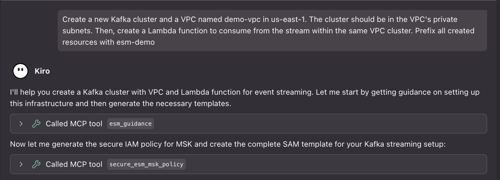
Imagine you want to set up a Lambda function to process events from an Amazon MSK cluster. Start by prompting your AI assistant:

Create a new Kafka cluster and a VPC named <your-vpc-name> in <your-aws-region>. The cluster should be in the VPC’s private subnets. Then, create a Lambda function to consume from the stream within the same VPC cluster. Prefix all created resources with <your-prefix>.

AI prompt to create a new Kafka cluster and ESM

The agent uses the esm_guidance to receive tailored guidance based on your use case and performance requirements. The tool analyzes your intent and provides step-by-step instructions for setting up the ESM with optimal configurations.

Apart from creating deployment and initialization scripts and supporting documentation, properly configured IAM polices and security groups rules to access the cluster are also generated. The assistant then validates the ESM parameters against AWS limits and best practices.

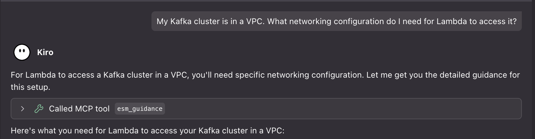
Next, you want to understand the networking requirements:

My Kafka cluster is in a VPC. What networking configuration do I need for Lambda to access it?

AI assistant prompt for setting up Kafka ESM networking connectivity

The Serverless MCP Server provides specialized guidance for VPC-based Kafka configurations using the esm_guidance tool with guidance_type=”networking”. This guidance provides detailed information about subnet requirements, security group rules, and NAT gateway setup, and it validates your network topology for reliable connectivity.

Optimizing event source mapping performance

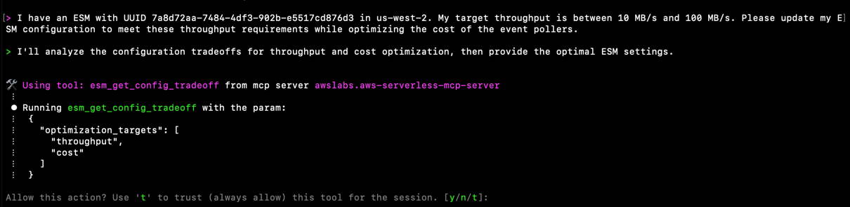
After your ESM is running, you notice that processing latency is higher than expected. You can ask for optimization guidance:

I have an ESM with UUID <your-esm-uuid> in <your-aws-region>. My target throughput is between 10 MB/s and 100 MB/s. Please update my ESM configuration to meet these throughput requirements while optimizing the cost of the event pollers.

AI prompt to optimize Kinesis ESM throughput
The server uses the esm_optimize tool to analyze your current configuration and provide optimization recommendations. The tool supports three main actions:

  • Analysis mode: (action="analyze") Analyzes configuration tradeoffs for your optimization targets (throughput, latency, cost, failure rate)
  • Validation mode: (action="validate") Validates your ESM configuration against AWS limits and event source restrictions
  • Template generation: (action="generate_template") Creates updated AWS SAM templates with optimized configurations

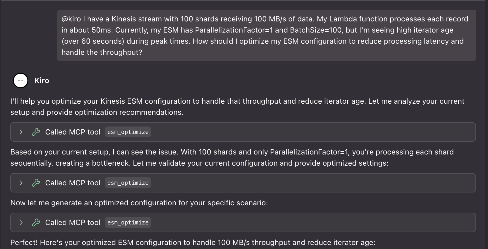
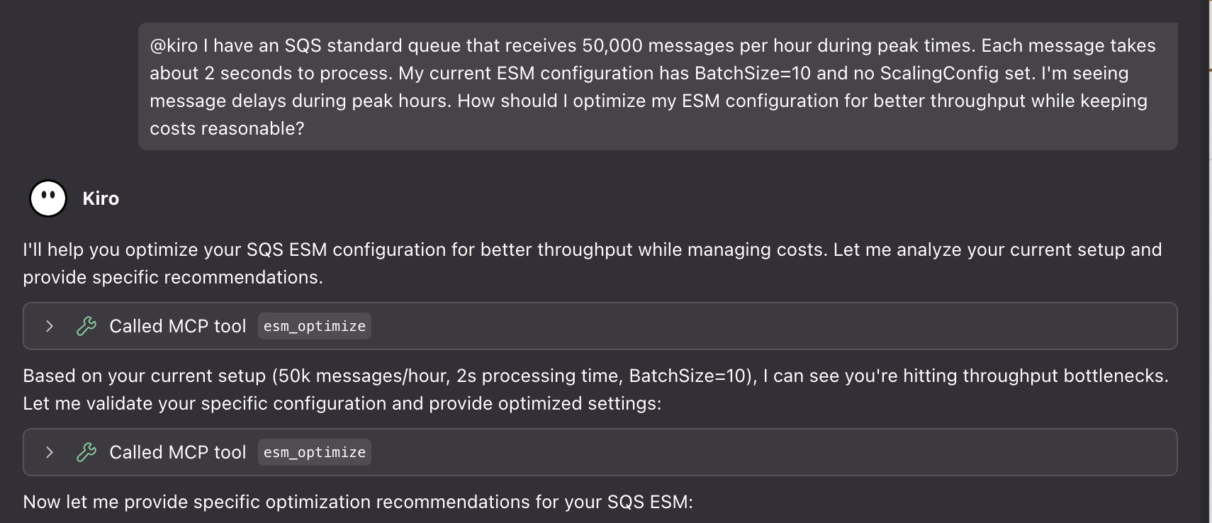
You can use this tool to get guidance on your event source mapping configurations for Amazon SQS, Amazon Kinesis Data Streams, and Amazon DynamoDB Streams. Here are two examples:

I have a Kinesis stream with 100 shards receiving 100 MB/s of data. My Lambda function processes each record in about 50ms. Currently, my ESM has ParallelizationFactor=1 and BatchSize=100, but I’m seeing high iterator age (over 60 seconds) during peak times. How should I optimize my ESM configuration to reduce processing latency and handle the throughput?

AI prompt to optimize Kinesis ESM throughput

I have an SQS standard queue that receives 50,000 messages per hour during peak times. Each message takes about 2 seconds to process. My current ESM configuration has BatchSize=10 and no ScalingConfig set. I’m seeing message delays during peak hours. How should I optimize my ESM configuration for better throughput while keeping costs reasonable?

The tool generates updated AWS Serverless Application Model (AWS SAM) templates with the recommended configurations, making it easy to apply the changes through your deployment pipeline. However, it always requires explicit user confirmation before any deployment.

Troubleshooting event source mapping issues

When an issue arises, the ESM tools provide diagnostic capabilities. For example, if your ESM stops processing events:

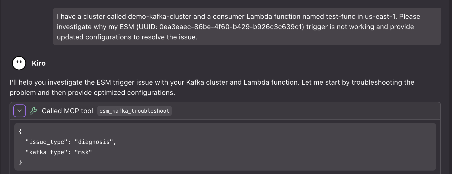
I have a cluster called <your-kafka-cluster-name> and a consumer Lambda function named <your-lambda-function-name>in <your-aws-region>. Please investigate why my ESM (UUID: <your-esm-uuid>) trigger is not working and provide updated configurations to resolve the issue.

AI assistant prompt for investigation an issue with Kafka ESM

The server uses the esm_kafka_troubleshoot tool to provide comprehensive troubleshooting for Apache Kafka clusters. The tool supports two main modes:

  • Diagnostic mode: (issue_type="diagnosis") Analyzes your ESM status and provides diagnostic indicators. This helps identify whether timeouts occur before or after reaching Kafka brokers. It categorizes issues into specific types for targeted resolution.
  • Resolution mode: Provides step-by-step resolution guidance for specific issues.

AI prompt to start debugging an issue with a Kafka ESM

The tool automatically detects your event source type and provides tailored guidance. It validates VPC connectivity, examines IAM permissions, checks security group configurations, and analyzes CloudWatch Logs to provide a detailed diagnosis report with specific remediation steps.

Key benefits

The event source mapping tools in the AWS Serverless MCP Server provide unique advantages over traditional event source mapping configuration approaches:

  • AI-powered configuration translation: The tools translate high-level developer intent (such as process 1,000 events per second) into specific ESM parameters like batch size, parallelization factor, and batching window.
  • Complete infrastructure-as-code generation: Unlike generic AWS CLI tools that provide individual commands, ESM tools generate complete AWS SAM templates, initialization scripts, cleanup scripts, and validation scripts for end-to-end automation.
  • Proactive network validation: For VPC-based event sources like Amazon MSK or self-managed Kafka, the tools validate network topology, security group rules, and connectivity before deployment, preventing common silent failures.
  • Context-aware troubleshooting: The diagnostic tools correlate ESM status, CloudWatch metrics, VPC configuration, and IAM permissions to provide comprehensive root cause analysis with specific remediation steps.

New tools available in the Serverless MCP Server

The event source mapping tools are designed to minimize trust permission prompts by using a small set of primary tools that internally call specialized functions. The tools can be classified into three main categories:

  • esm_guidance: This tool provides comprehensive guidance on creating and configuring event source mappings for all event sources (DynamoDB, Kinesis, Kafka, SQS). It handles setup, networking guidance, and troubleshooting based on the guidance_type parameter. The tool automatically generates AWS SAM templates, IAM policies, and security group configurations.
  • esm_optimize: This advanced optimization tool analyzes configuration tradeoffs, validates ESM settings, and generates AWS SAM templates for performance tuning. It supports three actions:
    • analyze: Provides configuration tradeoff analysis for failure rate, latency, throughput, and cost optimization
    • validate: Validates ESM configurations against AWS limits and event source restrictions
    • generate_template: Creates AWS SAM templates with optimized configurations
  • esm_kafka_troubleshoot: This specialized troubleshooting tool for Kafka ESM issues supports both Amazon MSK and self-managed Apache Kafka clusters. It also provides diagnostic capabilities and step-by-step resolution guidance for connectivity, authentication, and network issues.

The primary tools internally call specialized helper functions to provide comprehensive functionality that help generate IAM polices, security groups, scaling and concurrency configurations, and validate configurations.

Visit the Serverless MCP Server documentation for the full list of tools and resources.

Best practices and considerations

When building event-driven applications with the AWS Serverless MCP Server, start by using its guidance tools for architectural decisions. The server helps you choose appropriate event sources, understand networking requirements, and configure optimal settings based on your performance goals.For Kafka-based ESMs, pay special attention to VPC configuration. Use the server’s network troubleshooting tools to validate connectivity before deployment. The server can detect common issues like missing NAT gateways, incorrect security group rules, or subnet routing problems.Monitor your event source mappings continuously using the server’s diagnostic tools. Set up alerts for key metrics like iterator age, error rates, and throttling. The server can help you interpret these metrics and recommend configuration adjustments to maintain optimal performance.

Conclusion

The new event source mapping tools in the open-source AWS Serverless MCP Server simplify event source mapping management throughout the development lifecycle, from initial setup to ongoing optimization and troubleshooting. By combining AI assistance with ESM expertise, it helps developers build and deploy event-driven applications more efficiently while avoiding common configuration pitfalls.

As organizations continue to adopt event-driven serverless computing, tools that simplify ESM management and accelerate delivery become increasingly valuable.

To get started, visit the GitHub repository and explore the documentation. Share your experiences and suggestions through the GitHub repository to improve the MCP server’s capabilities and help shape the future of AI-assisted event-driven development.

For more serverless learning resources, visit Serverless Land.

Processing Amazon S3 objects at scale with AWS Step Functions Distributed Map S3 prefix

Post Syndicated from Biswanath Mukherjee original https://aws.amazon.com/blogs/compute/processing-amazon-s3-objects-at-scale-with-aws-step-functions-distributed-map-s3-prefix/

If you’re building large scale enterprise applications, you’ve likely faced the complexities of processing large volumes of data files. Whether you’re analyzing your application logs, processing customer data files, or transforming machine learning datasets, you know the complexity involved in orchestrating workflows. You’ve probably written nested workflows and additional custom code to process objects from Amazon Simple Storage Service (Amazon S3) buckets.

With AWS Step Functions Distributed Map, you can process large scale datasets by running concurrent iterations of workflow steps across data entries in parallel, achieving massive scale with simplified management.

With the new prefix-based iteration feature and LOAD_AND_FLATTEN transformation parameter for Distributed Map, your workflows can now iterate over S3 objects under a specified prefix using S3ListObjectsV2 to process their contents in a single Map state, avoiding nested workflows and reducing operational complexity.

In this post, you’ll learn how to process Amazon S3 objects at scale with the new AWS Step Functions Distributed Map S3 prefix and transformation capabilities.

Use case: Application log processing and summarization

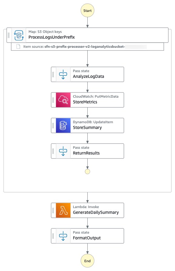
You’ll build a sample Step Functions state machine that demonstrates processing of all the log files from the given S3 prefix using a Distributed Map. You’ll analyze all the log files to build a summary INFO, WARNING and ERROR messages in the log file on hourly basis. The following diagram presents the AWS Step Functions state machine:

Log files processing workflow

Log files processing workflow

  1. The state machine iterates over all the log files from the specified S3 prefix using S3 ListObjectsV2 and process them using AWS Step Functions Distributed Map.
  2. For each log file entry, the state machine puts hourly ErrorCount metric into Amazon CloudWatch.
  3. The state machine then stores hourly metrics count in a Amazon DynamoDB table.
  4. The state machine then invokes an AWS Lambda function to perform metrics aggregation.

The following is an example of the parameters in an ItemReader configured to iterate over the content of S3 objects using S3 ListObjectsV2.

{
  "QueryLanguage": "JSONata",
  "States": {
    ...
    "Map": {
        ...
        "ItemReader": {
            "Resource": "arn:aws:states:::s3:listObjectsV2",
            "ReaderConfig": {
                // InputType is required if Transformation is LOAD_AND_FLATTEN. Use one of the given values
                "InputType": "CSV | JSON | JSONL | PARQUET",
                // Transformation is OPTIONAL and defaults to NONE if not present
                "Transformation": "NONE | LOAD_AND_FLATTEN" 
            },
            "Arguments": {
                "Bucket": "amzn-s3-demo-bucket1",
                "Prefix": "{% $states.input.PrefixKey %}"
            }
        },
        ...
    }
}

With the LOAD_AND_FLATTEN option, your state machine will do the following:

  1. Read the actual content of each object listed by the Amazon S3 ListObjectsV2 call.
  2. Parse the content based on InputType (CSV, JSON, JSONL, Parquet).
  3. Create items from the file contents (rows/records) rather than metadata.

We recommend including a trailing slash on your prefix. For example, if you select data with a prefix of folder1, your state machine will process both folder1/myData.csv and folder10/myData.csv. Using folder1/ will strictly process only one folder. All of the objects listed by prefix need to be in the same data format. For example, if you are selecting InputType as JSONL, your S3 prefix should contain only JSONL files and not a mix of other types.

The context object is an internal JSON structure that is available during an execution. The context object contains information about your state machine and execution. Your workflows can reference the context object in a JSONata expression with $states.context.

Within a Map state, the context object includes the following data:

"Map": {
   "Item": {
      "Index" : Number,
      "Key"   : "String", // Only valid for JSON objects
      "Value" : "String",
      "Source": "String"
   }
}

For each Map iteration, the Index contains the index number for the array item that is being currently processed.

A Key is only available when iterating over JSON objects. Value contains the array item being processed. For example, for the following input JSON object, Names will be assigned to Key and {"Bob", "Cat"} will be assigned to Value.

{
	"Names": {"Bob", "Cat"}
} 

Source contains one of the following:

  • For state input: STATE_DATA
  • For Amazon S3 LIST_OBJECTS_V2 with Transformation=NONE, the value will show the S3 URI for the bucket. For example: S3://amzn-s3-demo-bucket1
  • For all the other input types, the value will be the Amazon S3 URI. For example: S3://amzn-s3-demo-bucket1/object-key

Using LOAD_AND_FLATTEN and the Source field, you can connect child executions to their sources.

Prerequisites

Set up and run the workflow

Run the following steps to deploy and test the Step Functions state machine.

  1. Clone the GitHub repository in a new folder and navigate to the project folder.
    git clone https://github.com/aws-samples/sample-stepfunctions-s3-prefix-processor.git
    cd sample-stepfunctions-s3-prefix-processor

  2. Run the following commands to deploy the application.
    sam deploy --guided

  3. Enter the following details:
    • Stack name: Stack name for CloudFormation (for example, stepfunctions-s3-prefix-processor)
    • AWS Region: A supported AWS Region (for example, us-east-1)
    • Accept all other default values.

    The outputs from the AWS SAM deploy will be used in the subsequent steps.

  4. Run the following command to generate sample log files.
    python3 scripts/generate_logs.py

  5. Run the following to upload the log files to the S3 bucket with the /logs/daily prefix. Replace amzn-s3-demo-bucket1 with the value from the sam deploy output.
    aws s3 sync logs/ s3://amzn-s3-demo-bucket1/logs/ --exclude '*' --include '*.log'

  6. Run the following command to execute the Step Functions workflow. Replace the StateMachineArn with the value from the sam deploy output.
    aws stepfunctions start-execution \
      --state-machine-arn <StateMachineArn> \
      --input '{}'

    The Step Function state machine iterates over all the log files with the S3 prefix /logs/daily and processes them in parallel. The workflow updates the metrics in CloudWatch, stores hourly metrics count in DynamoDB, then invokes an AWS Lambda function to aggregate the metrics.

Monitor and verify results

Run the following steps to monitor and verify the test results.

  1. Run the following command to get the details of the execution. Replace executionArn with your state machine ARN.
    aws stepfunctions describe-execution --execution-arn <executionArn>

  2. When the status shows SUCCEEDED, run the following commands to check the processed output from the LogAnalyticsSummaryTableName DynamoDB table. Replace the value LogAnalyticsSummaryTableName with the value from the sam deploy output.
    aws dynamodb scan --table-name <LogAnalyticsSummaryTableName>

  3. Check that hourly ERROR, WARN, and INFO logs statistics are saved in the DynamoDB table. The following is a sample output:
    {
        "Items": [
            {
                "ProcessingTime": {
                    "S": "2025-10-07T23:45:10.790Z"
                },
                "WarningCount": {
                    "N": "2"
                },
                "HourOfDay": {
                    "S": "13"
                },
                "TotalRecords": {
                    "N": "5"
                },
                "ErrorCount": {
                    "N": "3"
                },
                "InfoCount": {
                    "N": "0"
                },
                "HourKey": {
                    "S": "2025-10-08 13"
                }
            },
            {
                "ProcessingTime": {
                    "S": "2025-10-07T23:45:07.456Z"
                },
                "WarningCount": {
                    "N": "3"
                },
                "HourOfDay": {
                    "S": "09"
                },
                "TotalRecords": {
                    "N": "6"
                },
                "ErrorCount": {
                    "N": "2"
                },
                "InfoCount": {
                    "N": "1"
                },
                "HourKey": {
                    "S": "2025-10-08 09"
                }
            },
            …
    ],
        "Count": 24,
        "ScannedCount": 24,
        "ConsumedCapacity": null
    }

  4. Run the following command to check the output of the Step Functions state machine execution output.
    aws stepfunctions describe-execution --execution-arn <executionArn> --query 'output' --output text

    The following is a sample output:

    {
      "Summary": {
        "date": "2025-10-08",
        "totalErrors": 50,
        "totalWarnings": 41,
        "totalRecords": 133,
        "hourlyBreakdown": {
          "00": {
            "errors": 1,
            "warnings": 3,
            "records": 5
          },
          "01": {
            "errors": 1,
            "warnings": 1,
            "records": 5
          },
          "02": {
            "errors": 2,
            "warnings": 3,
            "records": 5
          },
          "03": {
            "errors": 3,
            "warnings": 2,
            "records": 7
          },
    …
    …
        "generatedAt": "2025-10-08T05:19:05.603889"
      }
    }

    The output of the Step Functions state machine shows the daily summary insights of the log files created by the Lambda function.

Clean up

To avoid costs, remove all resources created for this post once you’re done. Run the following command after replacing amzn-s3-demo-bucket1 with your own bucket name to delete the resources you deployed for this post’s solution:

aws s3 rm s3://amzn-s3-demo-bucket1 --recursive
sam delete
rm -rf logs/

Conclusion

In this post, you learned how AWS Step Functions Distributed Map can use prefix-based iteration with LOAD_AND_FLATTEN transformation to read and process multiple data objects from Amazon S3 buckets directly. You no longer need one step to process object metadata and another to load the data objects. Loading and flatting in one step is particularly valuable for data processing pipelines, batch operations, and event-driven architectures where objects are continually added to S3 locations. By eliminating the need to maintain object manifests, you can build more resilient, dynamic data processing workflows with less code and fewer moving parts.

New input sources for Distributed Map are available in all commercial AWS Regions where AWS Step Functions is available. To get started, you can use the Distributed Map mode today in the AWS Step Functions console. To learn more, visit the Step Functions developer guide.

For more serverless learning resources, visit Serverless Land.

Breaking down monolith workflows: Modularizing AWS Step Functions workflows

Post Syndicated from Sahithi Ginjupalli original https://aws.amazon.com/blogs/compute/breaking-down-monolith-workflows-modularizing-aws-step-functions-workflows/

You can use AWS Step Functions to orchestrate complex business problems. However, as workflows grow and evolve, you can find yourself grappling with monolithic state machines that become increasingly difficult to maintain and update. In this post, we show you strategies for decomposing large Step Functions workflows into modular, maintainable components. We dive deep into architectural patterns like parent-child workflows, domain-based separation, and shared utilities that can help you break down complexity while maintaining business functionality. By implementing these decoupling techniques, you can achieve faster deployments, better error isolation, and reduced operational overhead – all while keeping your workflows scalable and efficient. Whether you’re dealing with payment processing, data transformation, or complex business logic, these patterns will help you build more resilient and manageable Step Functions applications.

The Complexity of Single-State Machine Architectures

While monolithic workflows can be suitable for simple, linear processes with limited states and clear dependencies, they become problematic when handling complex business logic across multiple domains. If your workflow involves more than 15-20 states, crosses multiple business domains, or requires frequent updates from different teams, it’s a strong indicator that you should consider a decomposed approach instead of a monolithic one. However, monolithic workflows remain a valid choice for scenarios with straightforward business logic, single-team ownership, infrequent changes, and workflows with less than 15 states – especially when rapid development and simplified debugging are priorities.

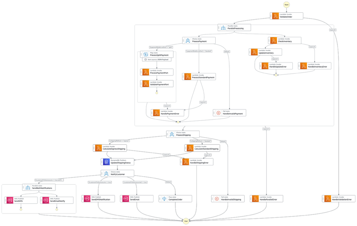
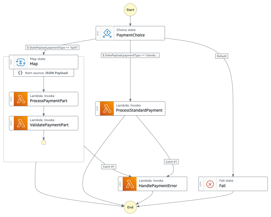
Let’s examine a real-world example of such a monolithic workflow and understand the challenges it presents for development teams, operational efficiency, and business agility. Below is an example of a state machine that is a mix of payment processes, inventory management, and notification mechanisms for an e-commerce implementation:

Figure 1: A state machine that is a mix of payment processes, inventory management, and notification mechanisms for an e-commerce implementation

Figure 1: A state machine that is a mix of payment processes, inventory management, and notification mechanisms for an e-commerce implementation

State Explosion

Modifying a single state in a monolithic workflow triggers a cascade of changes across multiple interconnected states due to their tight coupling and dependencies. For example, adding a new payment method would require modifications across various states including validation, processing, and error handling, creating a ripple effect throughout the workflow. This inter dependency makes even simple changes complex and risky, as altering one component can have unintended consequences on other parts of the workflow.

Looking at the provided architecture, we can see a clear example of state explosion where a single workflow handles multiple business processes including order validation, payment processing, inventory management, shipping calculations, and customer notifications. This creates a complex web of dependent states that becomes increasingly difficult to manage. The result is a “spider web” of states that becomes progressively harder to understand, debug, and maintain.

Version Management

Version management in monolithic workflows requires deploying the entire workflow even for minor changes to individual components, making it difficult to isolate and update specific business logic. The provided architecture demonstrates the version management challenge clearly. For instance, if the shipping calculation logic needs an urgent fix, the entire workflow must be redeployed, requiring comprehensive testing of all components, including unmodified ones, to ensure nothing breaks in the process.

Resource Limitations

While not immediately visible in the architecture diagram, Monolithic workflows face operational constraints as they grow in complexity, particularly with state transitions, maximum event payload size, and execution history size. Refer to the Service quotas documentation to understand such limits. These constraints become critical bottlenecks as workflows grow in complexity and handle increased transaction volumes. In the monolithic state machine, long-running operations like payment processing and shipping calculations, combined with multiple state transitions, could approach these limits, especially for high-volume scenarios.

Additionally, we also come across generic design challenges such as error handling. In monolithic approach, workflows leads to redundant try-catch blocks and retry configurations across different operations. This creates challenges in implementing distinct error strategies for different business scenarios and makes it difficult to maintain proper rollback mechanisms when failures occur in middle states.

These challenges collectively highlight the need for a more modular approach to Step Functions workflow design.

Transforming Complex Workflows Through Decomposition

When transforming complex monolithic workflows into more manageable components, you can employ several decomposition strategies to achieve better modularity and maintainability. These strategies include the parent-child pattern, which creates a hierarchical structure of workflows, domain separation that breaks down workflows based on business capabilities, shared utilities that serve as reusable components for common operations, and specialized error workflows for centralized error handling. Each of these strategies can be implemented either individually or in combination, depending on the specific requirements and complexity of the application, allowing organizations to create more efficient, scalable, and maintainable Step Functions workflows while ensuring proper separation of concerns and reduced operational overhead.

Parent-Child Pattern

The parent-child pattern represents a hierarchical approach to workflow organization where a main (parent) workflow orchestrates multiple sub-workflows (children). Parent workflows manage the overall business process and coordination, while child workflows handles specific, short-lived operations. This pattern is particularly effective when you need to balance between orchestration complexity and execution speed.

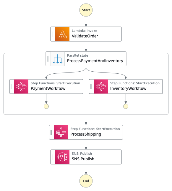
 Figure 2 : Decoupled parent state machine

Figure 2 : Decoupled parent state machine

The current monolithic workflow can be restructured by creating a parent workflow focused on order orchestration while delegating specific operations to Express child workflows. The parent workflow would maintain the high-level flow from order validation through completion, while time-sensitive operations like ValidateOrder, ProcessPayment, and ProcessShipping could become Express child workflows.

Kindly note that during an architecture re-vamp, Express workflows are different when compared to Standard Workflows. For example, you cannot have an Express parent workflow invoke a Standard child workflow. Also, an Express workflow does not support Job-run (.sync) or Callback (.waitForTaskToken) service integration patterns. You can refer to the differences between Standard and Express workflows documentation to choose the right architecture pattern.

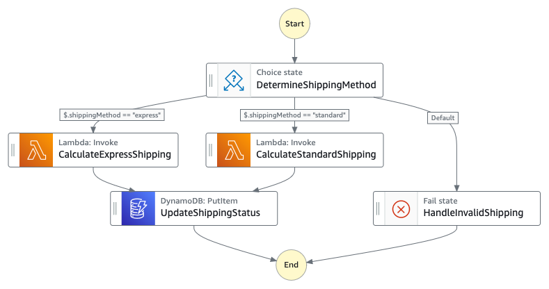
For instance, the payment processing section could be transformed into a child Express workflow that handles all payment-related states (ProcessPayment, ProcessStandardPayment, ValidatePaymentPart) as a single unit. An express workflow is more suitable for sections like payment processing as their executions complete within 5 minutes. Hence this would also reduce the over-all cost of the workflow. Similarly, the shipping calculation logic involving CalculateExpressShipping and CalculateStandardShipping could be consolidated into another Express child workflow, leading to reduced costs and easier updates to shipping logic.

Domain Separation

Domain separation involves breaking down workflows based on distinct business capabilities or functional areas. Each domain-specific workflow becomes responsible for a complete business function, operating independently while communicating through well-defined interfaces. This approach aligns closely with micro-service architecture principles and domain-driven design. The architecture shows clear boundaries between different business domains that can be separated into independent workflows. Three primary domains emerge:

  1. Payment Domain: Encompassing ValidateOrder, ProcessPayment, ValidatePaymentPart, and related error handlers
  2. Inventory Domain: Including CheckInventory, UpdateInventory, and associated states
  3. Shipping Domain: Containing ProcessShipping, shipping calculations, and shipping status updates

Each domain would become its own workflow, with clear input/output contracts. This separation would allow specialized teams to maintain and deploy updates to their domain workflows independently ensuring implementation of domain-specific retry policies, error handling, and business rules without affecting other domains. For example, the payment team could enhance payment processing logic without impacting shipping or inventory operations.

 Figure 3 : Child state machine that handles payment workflow

Figure 3 : Child state machine that handles payment workflow

 Figure 4 : Child state machine that handles shipping workflow

Figure 4 : Child state machine that handles shipping workflow

Shared Utilities

Shared utility workflows serve as reusable components for common operations that appear across multiple business processes. These workflows encapsulate standard functionality like notification handling, data validation, logging, or audit trail creation. By centralizing these common operations, organizations can ensure consistency and reduce duplication across their Step Functions applications.

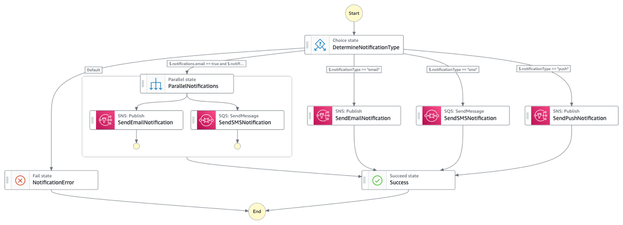
The current architecture repeats several common patterns that could be extracted into shared utility workflows. Most notably, the notification handling logic (SendEmail, SendSMSNotification, SendPushNotification) appears as a cluster of states at the end of the workflow. This could be consolidated into a single “NotificationManager” utility workflow that handles all types of notifications. These utility workflows could then be called from any other workflow in the system, ensuring consistent behavior and reducing code duplication.

 Figure 5 : Re-usable notification workflow

Figure 5 : Re-usable notification workflow

Error Workflows

Error workflows represent a specialized form of decomposition focused on centralizing error handling and recovery logic. Instead of embedding complex error handling in each business workflow, organizations can create dedicated workflows that manage different types of failures, retries, and compensation actions. This approach provides a consistent and maintainable way to handle errors across the application.

Each of these decomposition strategies can be used individually or in combination, depending on the specific needs of your application. For instance, utilization of Domain Separation pattern has resulted in streamlined error workflows. The key is to choose the appropriate combination that provides the right balance of maintainability, scalability, and operational efficiency for your use case. However, implementing all four strategies in a phased approach would provide the most comprehensive solution for long-term maintainability and scalability.

Results:

The comparison between monolithic and decoupled approaches reveals notable differences in performance and operational metrics. In order to emulate similar test environments across monolithic and decomposed state machines, we tested them in us-east-1 AWS region. We made use of the aforementioned workflows, both monolithic and decomposed to achieve a similar end goal. Pricing comparison is based on a monolithic workflow processing 11 state transitions per workflow across 30,000 monthly requests. For the decomposed approach, calculations assume Express child workflows configured with 64MB memory and 100ms execution duration, while the parent workflow handles 8 state transitions per workflow for the same volume of 30,000 monthly requests. AWS Lambda task states in both approaches complete within 2 seconds of execution time.

When decoupled, the workflows can be re-designed to use either Express or Standard mechanisms depending on their execution time and integration pattern requirements. In this use-case, we identified multiple workflows like PaymentProcessing, CalculateExpressShipping that are revamped to use Express workflows as per their requirement. While the monolithic approach shows a slightly faster execution duration of 11.5 seconds compared to 13 seconds in the decomposed approach, the monthly pricing significantly favors the decoupled architecture at $6.37 USD versus $11.90 USD for the monolithic approach. The decoupled approach demonstrates superior debugging capabilities with better error isolation and domain-specific debugging, contrasting with the monolithic approach’s complex debugging challenges due to heavy payloads and middle-state failure tracking. Additionally, the decoupled architecture benefits from smaller payload sizes through distributed data handling, whereas the monolithic workflow carries larger payloads across its 18 state transitions.


Monolithic Approach Decoupled Approach
Execution Duration 11.5 seconds for complete workflow execution 13 seconds with distributed processing across parent-child workflows
Monthly Pricing $11.90 USD (476,000 billable state transitions) $6.37 USD (Combined cost of Standard parent workflow and Express child workflows)
Debug Effort High – Complex debugging due to heavy payloads and difficulty in tracking failures in middle states. Cannot effectively use ResultSelector when final notification state needs all details. Lower – Easier to debug with isolated domains and smaller payloads. Better error isolation and domain-specific debugging.
Payload Size Larger payload size throughout workflow execution as all data needs to be carried across 18 state transitions Smaller payload size due to domain separation and distributed data handling across parent-child workflows

Conclusion

The need for decomposing Step Functions workflows becomes evident when you face challenges with monolithic workflows such as state explosion, version management complexities, and resource limitations. These challenges result in reduced operational efficiency, increased debugging complexity, and higher maintenance overhead as demonstrated by the comparison results showing differences in execution duration, pricing, debugging effort, and payload management. Organizations should evaluate workflow decomposition when they observe workflows exceeding 15-20 states, multiple team involvement in workflow maintenance, frequent independent updates across different business domains, complex error handling requirements, and the need for reusable components across workflows. The implementation of decomposition strategies through parent-child pattern for hierarchical workflow organization, domain separation for business capability isolation, shared utilities for common operations, and dedicated error workflows for centralized error handling has shown tangible benefits in terms of reduced costs, better error isolation, and more efficient payload management.

While implementing decomposition strategies, organizations must be cautious to avoid over-decomposition of workflows, maintaining tight coupling between workflows, and ignoring core design principles of loose coupling and single responsibility. This strategic approach to workflow decomposition ultimately leads to more maintainable, scalable, and cost-effective Step Functions applications that better serve business needs while reducing operational overhead. The transformation from monolithic to decomposed workflows represents a significant architectural improvement that enables organizations to better manage complex business processes while maintaining operational efficiency and system reliability.

BASF Digital Farming builds a STAC-based solution on Amazon EKS

Post Syndicated from Kevin S. Ridolfi original https://aws.amazon.com/blogs/architecture/basf-digital-farming-builds-a-stac-based-solution-on-amazon-eks/

This post was co-written with Frederic Haase and Julian Blau with BASF Digital Farming GmbH.

At xarvio – BASF Digital Farming, our mission is to empower farmers around the world with cutting-edge digital agronomic decision-making tools. Central to this mission is our crop optimization platform, xarvio FIELD MANAGER, which delivers actionable insights through a range of geospatial assets, including satellite imagery, drone data, and application maps from sprayers.

In this post, we show you how we built a scalable geospatial data solution on AWS to efficiently catalog, manage, and visualize both raster and vector datasets through the web. We walk you through our solution based on the SpatioTemporal Asset Catalog (STAC) specification and the open source eoAPI ecosystem, detailing the solution architecture, key technologies, and lessons learned during deployment. This builds upon a previous post on efficient satellite imagery ingestion using AWS Serverless, extending our discussion to the full lifecycle of geospatial data management at scale.

Requirements for our geospatial data solution

BASF Digital Farming’s xarvio FIELD MANAGER platform operates at exceptional scale in the geospatial data ecosystem, processing hundreds of millions of satellite images that translate into STAC items, which further decompose into billions of individual geospatial artifacts. Unlike traditional satellite data providers such as European Space Agency (ESA) who work with predictable, structured data flows, we operate in an inherently dynamic agricultural environment where we ingest near-daily satellite imagery per field from a diverse array of sensors and providers globally. Our mission to support farmers worldwide with advanced digital agronomic decision advice demands a reliable, cloud-based infrastructure capable of handling this massive data velocity and volume and applying advanced quality assurance processes including cloud detection and anomaly detection algorithms. The platform’s true value emerges through our machine learning (ML) pipelines that transform raw satellite data into actionable insights. For example, estimating accurate absolute biomass such as Leaf Area Index (LAI) helps farmers make precise, data-driven agronomic decisions that optimize crop yield and resource utilization across fields worldwide.

STAC and eoAPI ecosystem

To efficiently manage our growing archive of geospatial data, we adopted the Spatio Temporal Asset Catalog (STAC) specification, an open standard that provides a common language to describe and catalog raster and vector datasets. With STAC, we can standardize metadata across diverse sources like satellite imagery, UAV datasets, and prescription maps, making it straightforward to search, filter, and retrieve assets across our platform. We built our platform using the eoAPI ecosystem, an integrated suite of open source tools designed to handle the full lifecycle of geospatial data on the cloud. At its core is pgSTAC, which provides a performant PostGIS-backed STAC API implementation. With pgSTAC, we can index millions of STACi Items efficiently, with support for spatial, temporal, and attribute-based filtering at scale. On top of that, we use Tiles in PostGIS (TiPG) to serve tiled vector data directly from our PostGIS database. This enables real-time visualization of field boundaries, management zones, and application histories as lightweight Mapbox Vector Tiles (MVT), without requiring an external tile server. For raster assets, including satellite and drone imagery, we rely on TiTiler, a modern dynamic tile server built for Cloud Optimized GeoTIFFs (COGs). With TiTiler, we can stream imagery on-demand as WMTS or XYZ tiles, perform dynamic rendering (such as NDVI or false color composites), and integrate seamlessly into web maps and mobile apps.

Solution overview

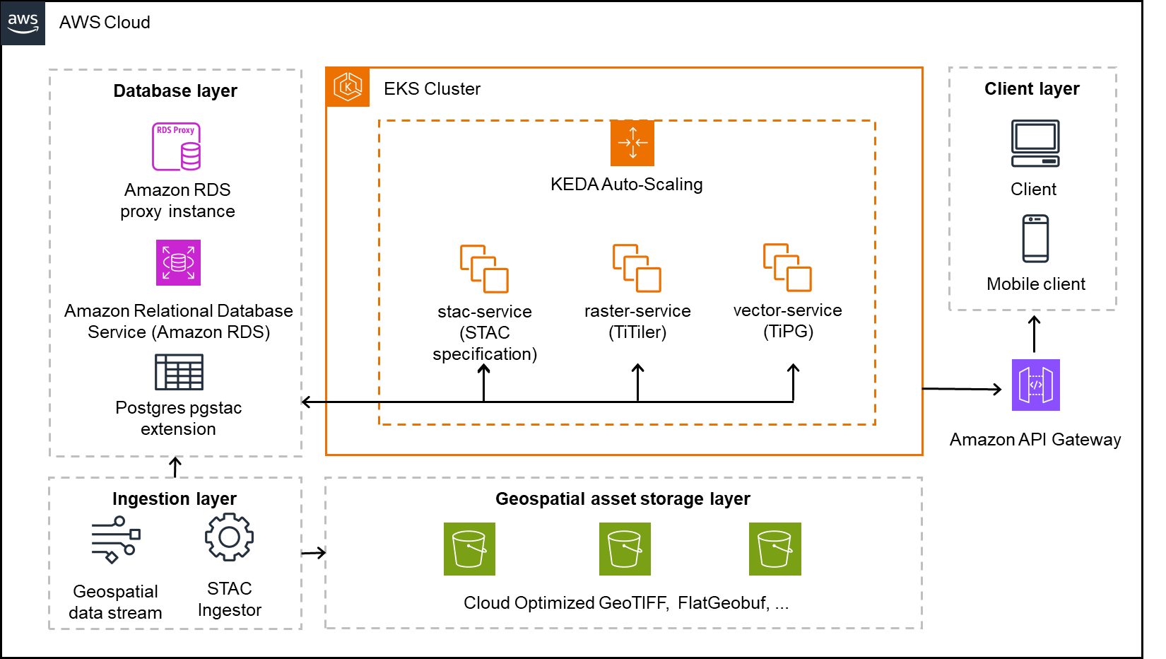
The following architecture diagram shows how we implemented our geospatial data platform on AWS. In this section, we explain each component of the architecture and how they work together to process millions of satellite images and geospatial assets daily. The solution uses Amazon Elastic Kubernetes Service (Amazon EKS) as the core computing platform, with Amazon Simple Storage Service (Amazon S3) for storage and Amazon Relational Database Service (Amazon RDS) for metadata management. We break down the architecture into four main layers: core services, storage, database, and ingestion.

A detailed AWS Cloud architecture visualization showcasing a complete geospatial data processing system across four distinct layers. The database layer features an EKS Cluster managing STAC, raster, and vector services, all connected to Amazon RDS through a proxy instance. The client layer supports both desktop and mobile access via Amazon API Gateway. The ingestion layer processes geospatial data streams through a STAC ingestor, feeding into a robust storage layer utilizing Cloud Optimized GeoTIFF and FlatGeobuf technologies. The architecture emphasizes scalability and efficient spatial data handling through PostgreSQL with pgstac extension, enabling seamless integration of various geospatial services and data formats.

Core services layer

The solution uses an EKS cluster hosting three key services:

  • stac-service – Implements the STAC API specification to catalog and serve metadata for both raster and vector datasets
  • raster-service – Powered by TiTiler, this service dynamically renders and tiles cloud-optimized raster data (for example, COGs) for seamless integration into web and mobile maps
  • vector-service – Built with TiPG, this component serves vector data (for example, boundaries or application zones) as tiled MVT layers directly from the database or from Amazon S3

These services are containerized and orchestrated within Kubernetes, allowing for high availability, modular separation, and simplified continuous integration and delivery (CI/CD) workflows.

KEDA-based automatic scaling

We use Kubernetes Event-Driven Autoscaling (KEDA) to scale our platform services dynamically based on real-time workloads. With KEDA, we can scale individual pods based on precise event-driven metrics such as the STAC ingestion queue depth or visualization request load. This supports responsive performance during peak activity while maintaining lean resource usage during idle periods, aligning perfectly with our need for elasticity in a data-intensive, variable-load environment.

Geospatial asset storage layer

The platform stores all raw and processed geospatial assets in S3 buckets, optimized for performance and durability. This layer holds COGs for raster imagery and FlatGeobuf or similar formats for vector data. These formats are chosen for their support of streaming access, indexing, and cloud-based performance.

Database layer

The metadata backbone of the system is a PostgreSQL database hosted on Amazon RDS, extended with the pgSTAC plugin. This setup enables efficient indexing and querying of millions of STAC items and collections. An RDS proxy sits in front of the database, providing connection pooling and resiliency, especially under bursty or concurrent access patterns common in geospatial applications.

Ingestion layer

An independent ingestion component handles batch or streaming geospatial data inputs. This component processes satellite imagery, drone data, or prescription maps and pushes relevant metadata into the STAC API and storage assets into Amazon S3. The ingestion engine is decoupled from serving infrastructure, enabling asynchronous and large-scale data loading.

Amazon API Gateway and clients

Public access to the platform is handled through Amazon API Gateway, allowing clients—whether browser-based or mobile—to interact securely with the services. The API gateway provides a unified entrypoint and is used for applying rate limiting, authorization, and routing policies.

Solution benefits

The solution offers the following benefits:

  • Rapid onboarding with STAC standardization – By aligning with the STAC specification, we’ve significantly reduced the time to onboard new data domains like sprayer application maps. Compared to previous approaches in our legacy system, metadata modeling and integration are now both standardized and automated, so we can expose new geospatial data products to clients in days instead of weeks or months.
  • Optimized storage with COGs and Amazon S3 – Storing raster and vector assets in Amazon S3 using cloud-optimized formats (such as COGs for imagery or FlatGeobuff for vectors) reduces storage costs while enabling low-latency, streaming access. This avoids the need for preprocessing or extract, transform, and load (ETL)-heavy pipelines and simplifies client delivery.
  • Large-scale ingestion with a batch STAC ingestor – Our custom STAC ingestor supports both real-time and batch-mode operations. This has made it possible to onboard satellite constellations, drone imagery, and historical datasets in bulk without disrupting running services. The ingestion service uses optimized database ingestion functions, capable of ingesting thousands of items per second, providing high-throughput and reliable data integration at scale.
  • PostgreSQL, pgSTAC, and Amazon RDS Proxy for a scalable metadata backbone – With pgSTAC and Amazon RDS Proxy, we benefit from advanced spatial-temporal querying while making sure database connection management is handled gracefully, even under high concurrency. This combination offers reliability without compromising performance.
  • Scalable deployment with Amazon EKS – Hosting the solution on Amazon EKS provides full control over deployments, resource tuning, and service orchestration. Combined with automatic scaling, we dynamically adjust compute capacity based on demand, facilitating resilience and cost-efficiency.

Learnings

As part of building this solution, we learned the following:

  • RDS Proxy is essential for automatically scaled environments – Given our use of automatic scaling pods in Amazon EKS, we found that RDS Proxy is critical. It handles connection pooling efficiently and protects the underlying PostgreSQL database from connection exhaustion during sudden scale-up events. Without it, we encountered spiky load failures and blocked connections during high-ingest periods.
  • Batch STAC ingestor is a core component – Our custom STAC ingestor proved to be an indispensable piece of the system. It interfaces directly with pgSTAC to perform large-scale, automated ingestions of geospatial metadata from streams and archives. Without this tool, onboarding data providers or processing legacy imagery at scale would have been labor-intensive and error-prone.
  • COGs are non-negotiable – For fast, scalable visualization of large raster datasets, COGs are essential, particularly if raster datasets exceed several gigabytes. They enable efficient HTTP range requests, alleviate the need for preprocessing, and work seamlessly with TiTiler for real-time tile rendering. Non-COG formats led to noticeably slower performance and weren’t suitable for cloud-based visualization.
  • Serverless-compliant, optimized for Amazon EKS (for now) – Although the architecture is designed to be serverless-compatible, we opted for an Amazon EKS first approach due to the nature of our other application landscape. Components like TiTiler and TiPG benefit from persistent, memory-tuned environments that are harder to achieve in a serverless runtime. However, the solution remains modular and stateless by design, and certain subsystems (such as ingestion triggers, notifications, or monitoring) are already candidates for future serverless migration to further improve elasticity and reduce operational overhead.

Conclusion

BASF Digital Farming GmbH has successfully implemented a STAC-based geospatial data platform on Amazon EKS, enabling efficient management and visualization of satellite imagery, drone data, and application maps. This architecture helps us onboard new data sources within weeks rather than months. The new platform also processes twice as much data in a single day while cutting costs by 50%, thanks to reduced data handling through the STAC schema and the efficiencies of automatic scaling. By adopting the STAC standard, the architecture improves data discoverability, reduces search latency, and supports more efficient analytic workflows.

Organizations looking to build similar geospatial data solutions can use AWS services like Amazon EKS, Amazon S3, and Amazon RDS along with open source tools like STAC and eoAPI to create scalable, cost-effective solutions. Learn more about building containerized applications on AWS at Containers on AWS.

Zero downtime blue/green deployments with Amazon API Gateway

Post Syndicated from Biswanath Mukherjee original https://aws.amazon.com/blogs/compute/zero-downtime-blue-green-deployments-with-amazon-api-gateway/

Modern applications require deployment strategies that minimize downtime and reduce risk. Blue/green deployment is a strategy that reduces downtime and risk by running two identical production environments called “blue” and “green”. At any given time, only one environment serves live production traffic while the other remains idle. This strategy provides immediate fallback to the previous stable version if issues arise after the new deployment. Let’s say a company is deploying a new version of its application. The following diagram shows the blue/green deployment strategy they are using.

Complete blue/green deployment strategy, including testing, monitoring, and conditional rollback procedures

As shown in the preceding diagram, current production traffic is served by the blue environment. During deployment of the new version of the application, the following sequence of activities happens:

  1. Deploy the new version of the application: Deploy the new version to the green environment.
  2. Test thoroughly: Test the new version in the green environment by invoking the API invoke URL from API Gateway. This does not affect production traffic, which continues to be served by the blue environment.
  3. Switch traffic: After you have thoroughly tested the green environment, redirect all production traffic from the blue to the green environment.
  4. Monitor and take any necessary action: Continue to monitor the green environment as it serves production traffic. Keep the blue environment ready for immediate rollback to the previous stable version, in case any issues arise in the green environment. At this point, one of two possible outcomes happens:
    1. If you identify any issues with the green environment in production, roll back to the previous stable version of the blue environment and fix the green environment before retrying.
    2. If you observe no issues with the green environment, decommission the blue environment. The green environment is now the new blue environment, the environment with stable production version of the application serving live traffic.

In this post, you learn how to implement blue/green deployments by using Amazon API Gateway for your APIs. For this post, we use AWS Lambda functions on the backend. However, you can follow the same strategy for other backend implementations of the APIs. All the required infrastructure is deployed by using AWS Serverless Application Model (AWS SAM).

Solution overview

As you follow along with this post, you will implement the following blue/green deployment architecture by using API Gateway custom domain API mapping. You use API mappings to connect API stages to a custom domain name. After you create a domain name and configure DNS records, you use API mappings to send traffic to your APIs through your custom domain name.

AWS serverless architecture showing blue /green deployment using Amazon API Gateway custom domain

As shown in the preceding diagram, the blue/green deployment architecture includes four primary AWS services – Amazon Route 53, Amazon API Gateway, AWS Lambda functions, and AWS Certificate Manager (ACM). When you send a request to the API, the Route 53 resolves the domain to the API Gateway custom domain. API Gateway handles HTTPS termination by using a configured ACM certificate. API Gateway examines the incoming request path and headers to route the request to the active environment.

You first set up the blue environment along with the Route 53 DNS configuration, API Gateway custom domain mapping, ACM and test it with Route 53 URL. This is your production environment serving live traffic. After that, deploy a new version of the application in the green environment and test it by invoking the API invoke URL from API Gateway while live traffic is still being served from the blue environment. Then, switch the traffic from the blue environment to the green environment by using API Gateway custom domain API mapping. This ensures that there is no change in the external (client-facing) API custom domain URL. Live traffic is now served by the green environment. If you observe any issues during this time, you can quickly roll back to the blue environment and fix the green environment. If the green environment is stable, you can decommission the blue environment.

This post uses two separate regional API endpoints to simulate blue/green environments and traffic routing between them but you can this same architectural pattern using single API endpoint with two stages representing blue and green environments.

Prerequisites

Complete the following prerequisites before you start setting up the solution:

Set up and test the solution

Note that this is a sample project to understand the concept and not for direct usage in production. The sample project contains three APIs.

  • Health GET API to know the current health of the environment and which environment the request was served from.
  • Pets GET API to get the list of available pets.
  • Order POST API to place a pet order.

Follow the steps below to setup blue/green deployment and test it.

  1. Clone the repository and navigate to the directory (all commands run from here)
    Clone the GitHub repository in a new folder and navigate to the stacks folder.

    git clone https://github.com/aws-samples/sample-blue-green-deployment-with-api-gateway.git
    cd sample-blue-green-deployment-with-api-gateway/stacks

  2. Deploy the blue environment
    You will first setup the blue environment. Run the following commands to deploy the blue environment:

    sam build -t blue-stack.yaml
    sam deploy -g -t blue-stack.yaml

    Enter the following details:

    • Stack name: The CloudFormation stack name (for example, blue-green-api-blue)
    • AWS Region: A supported AWS Region (for example, us-east-1)
    • BlueLambdaFunction has no authentication. Is this okay?: y
    • SAM configuration file: blue-samconfig.toml

    Keep everything else set to their default values. You will use the SAM deploy output for the subsequent steps. Going forward, you can run the following command to deploy the blue environment resources:

    sam build -t blue-stack.yaml
    sam deploy -t blue-stack.yaml --config-file blue-samconfig.toml

  3. Test the blue environment

    Run the following commands to test the blue environment after replacing ApiEndpoint with BlueApiEndpoint from the SAM deploy output in each case. First, test Health check API to know the health of the environment. Run the following command.

    curl --request GET \ 
    --url https://<ApiEndpoint>/health

    Sample response:

    {
      "status": "healthy", 
      "environment": "blue", 
      "version": "v1.0.0", 
      "timestamp": "2025-09-05T13:11:11.248267Z"
    }

    Second, test the pets GET API request to get the list of available pets. Run the following command.

    curl --request GET \ 
    --url https://<ApiEndpoint>/pets

    Sample response:

    {
      "environment": "blue",
      "version": "v1.0.0",
      "pets": [
        {
          "id": 1,
          "name": "Buddy",
          "category": "dog",
          "status": "available"
        },
        {
          "id": 2,
          "name": "Whiskers",
          "category": "cat",
          "status": "available"
        },
        {
          "id": 3,
          "name": "Charlie",
          "category": "bird",
          "status": "pending"
        }
      ]
    }

    Now, test create order POST API to place an order for a pet:

    curl --request POST \
      --url https://<ApiEndpoint>/orders \
      --header 'content-type: application/json' \
      --data '{
      "id": 1,
      "name": "Buddy"
    }'

    Expected response:

    {
      "confirmationNumber": "ORD-3251C0F4", 
      "environment": "blue",
      "version": "v1.0.0",
      "timestamp": "2025-09-05T13:16:04.703666Z", 
      "data": 
      {
        "id": 1, 
        "name": "Buddy", 
        "status": "ordered"
      }
    }
    

    Check that the response contains the environment attribute set to blue and the version attribute set to v1.0.0

  4. Deploy API Gateway custom domain pointing to the blue environment

    Run the following commands to deploy Amazon API Gateway custom domain with API mapping pointing to the blue environment created in the previous step.

    sam build -t custom-domain-stack.yaml
    sam deploy -g -t custom-domain-stack.yaml

    Enter the following details:

    • Stack name: (for example, blue-green-api-custom-domain)
    • AWS Region: A supported AWS Region (for example, us-east-1)
    • PublicHostedZoneId: The Route 53 public hosted zone ID (for example, ABXXXXXXXXXXXXXXXXXYZ)
    • CustomDomainName: The Route 53 domain name (for example, api.example.com)
    • CertificateArn: The ACM certificate ARN (for example, arn:aws:acm:us-east-1:123456789012:certificate/abc123)
    • ActiveApiId: The value of the BlueApiId output from the blue-stack deployment
    • ActiveApiStage: The value of the BlueApiStage output from the blue-stack deployment
    • SAM configuration file: custom-domain-samconfig.toml

    Keep everything else to their default values. You will use the SAM deploy output for the subsequent steps. At this point the production (live) traffic is routed to blue environment.

  5. Test the production (live) traffic which is routed to blue environment

    Follow the test method mentioned in step 3 to test the production environment, but replace ApiEndpoint with CustomDomainUrl. Check that the production environment response contains the environment attribute set to blue and the version attribute set to v1.0.0

  6. Deploy the green environment

    You will now deploy the v2.0.0 of the application on green environment. Run the following commands to deploy the green environment:

    sam build -t green-stack.yaml
    sam deploy -g -t green-stack.yaml

    Enter the following details:

    • Stack name: (for example, blue-green-api-green)
    • AWS Region: Select the same Region as the blue environment (for example, us-east-1)
    • GreenLambdaFunction has no authentication. Is this okay?: y
    • SAM configuration file: green-samconfig.toml

    Keep everything else to default values. You will use the SAM deploy output for the subsequent steps. Going forward, you can run the following commands to deploy the green environment.

    sam build -t green-stack.yaml
    sam deploy -t green-stack.yaml --config-file green-samconfig.toml
    

  7. Test the green environment
    Follow the test method shown in step 3 to test the production environment, but replace ApiEndpoint with GreenApiEndpoint. Validate that the response contains the environment attribute set to green and the version attribute set to v2.0.0
  8. Switch the live traffic to the green environment
    Run the following command to switch live traffic to the green environment:

    sam deploy -g -t custom-domain-stack.yaml  --config-file custom-domain-samconfig.toml

    Enter the following details:

    • Stack name: Keep it as it is.
    • AWS Region: Keep it as it is.
    • PublicHostedZoneId: Keep it as it is.
    • CustomDomainName: Keep it as it is.
    • CertificateArn: Keep it as it is.
    • ActiveApiId: The value of GreenApiEndpoint output from the green-stack deployment
    • ActiveApiStage: The value of GreenApiStage output from the green-stack deployment
    • SAM configuration file: Keep it as it is.

    Keep everything else at their default values.

  9. Test the production environment (now green) again

    Follow the test method shown in step 3 to test the production environment (now green) again, and be sure to replace ApiEndpoint with CustomDomainUrl from SAM deploy output. Validate that the response now contains the environment attribute set to green and the version attribute set to v2.0.0. Note that it may take a minute or two for the change to be seen due to local DNS caching, during this time some of the traffic may be still served from the blue environment. After switching the live traffic to the green environment, if there is an issue, you can switch the live traffic back to the blue environment and fix the green environment. Depending on whether you need to roll back to the previous stable blue environment or decommission the blue environment when you no longer need it, follow either step 10 or 11.

  10. (Option 1) Roll back to the blue environment, if necessary
    Run the following command to roll back to the blue environment, if necessary.

    sam deploy -g -t custom-domain-stack.yaml  --config-file custom-domain-samconfig.toml

    Enter the following details:

    • Stack name: Keep it as it is.
    • AWS Region: Keep it as it is.
    • PublicHostedZoneId: Keep it as it is.
    • CustomDomainName: Keep it as it is.
    • CertificateArn: Keep it as it is.
    • ActiveApiId: Value of BlueApiEndpoint output from the blue-stack deployment.
    • ActiveApiStage: The value of BlueApiStage output from the blue-stack deployment.
    • SAM configuration file: Keep it as it is.

    Keep everything else to their default values. Live traffic is switched to the blue environment. You can confirm that by following step 3.

  11. (Option 2) Decommission the blue environment when you no longer need it
    Run the following command to decommission (delete) the blue environment when you no longer need it. Replace blue-stack-name with your blue deployment stack name:

    sam delete --stack-name <blue-stack-name> --no-prompts

Clean up

To avoid costs, remove all resources created along this post once you’re done.

Run the following command after replacing the <placeholder> variables to delete the resources you deployed for this post’s solution:

# Delete all stacks (in reverse order)
# Delete custom domain
sam delete --stack-name <api-custom-domain-stack-name> --no-prompts
# Delete green stack
sam delete --stack-name <green-stack-name> --no-prompts
# Delete blue stack, if already not deleted in step 10
sam delete --stack-name <blue-stack-name> --no-prompts

Conclusion

Blue/green deployments with API Gateway provide a robust, scalable solution for zero-downtime deployments that deliver significant technical and operational advantages. This post’s solution architecture enables traffic switching at the API Gateway level while maintaining complete isolation between the blue and green environments to prevent interference. The solution offers immediate rollback capabilities for quick issue resolution and supports comprehensive testing through production-like validation before any traffic switching occurs.

Following this solution you can build a solid foundation for production blue/green deployments for your serverless microservice architecture that maintains the flexibility to adapt to your specific requirements while ensuring reliability, scalability, and operational excellence. To learn more about serverless architectures see Serverless Land.

Serverless ICYMI Q3 2025

Post Syndicated from Julian Wood original https://aws.amazon.com/blogs/compute/serverless-icymi-q3-2025/

Welcome to the 30th edition of the AWS Serverless ICYMI (in case you missed it) quarterly recap. At the end of a quarter, we share the most recent product launches, feature enhancements, blog posts, videos, live streams, and other interesting things that you might have missed!

In case you missed our last ICYMI, check out previous ICYMI posts.

Figure 1: Serverless calendar Q3 2025

Figure 1: Serverless calendar Q3 2025

GOTO Serverless Bengaluru

The Asia Serverless and GenAI Tour comprised 24 events across five countries. Cities included New Delhi, Bengaluru, Singapore, Manila, Bangkok, Perth, Melbourne, and Sydney. The GOTO Serverless conference in Bengaluru, India, formed the centerpiece with additional Developer Days, executive roundtables, user groups, cloud clubs, and specialized workshops. Thank you to all the developers who joined us on this incredible journey across Asia!

AWS Lambda

AWS Lambda now offers console to IDE integration and remote debugging capabilities that streamline the developer workflow from browser to Visual Studio Code and its clones. These enhancements reduce context switching and help developers debug Lambda functions directly in their preferred IDE environment.

The console to IDE feature provides an Open in Visual Studio Code button, enabling developers to move quickly from viewing their function in the browser to editing it in their IDE. AWS automatically handles setup, including the AWS Toolkit installation. Developers can also install dependencies and make code changes, which can automatically sync back to the cloud console. Watch the video to see how it works:

Remote debugging allows you to reduce debugging time from hours to minutes while simplifying local environment setups. You can set breakpoints and debug Lambda functions running in the actual cloud environment with complete access to Amazon VPC resources and AWS Identity and Access Management (AWS IAM) execution roles. The debugging connection uses AWS IoT Secure Tunneling Service, and AWS automatically cleans up debugging configuration after completion. Watch the video to see how it works:

Lambda now integrates with LocalStack directly in the AWS Toolkit for Visual Studio Code. This simplifies local testing of serverless applications involving multiple AWS services. You can now deploy serverless applications to LocalStack using the same commands, debug Lambda functions with one-click setup, and test end-to-end event-driven workflows locally before deploying to the cloud.

Lambda response streaming now supports a maximum response payload size of 200 MB, 10 times higher than before. Response streaming helps build applications that progressively stream response payloads back to clients, improving performance for latency-sensitive workloads by reducing time to first byte (TTFB) performance.

AWS Lambda Hackathon

The AWS Lambda Hackathon, challenged developers to build serverless applications solving real-world business problems using Lambda. With 3,732 participants and 331 project submissions, the competition showcased innovative serverless solutions across diverse domains.

Figure 2: AWS Lambda Hackathon

Figure 2: AWS Lambda Hackathon

We announced winners on July 22, 2025, with $15,000 in total prizes awarded:

  • First Place ($6,000): ForestShield: AWS Deforestation Detection by Younes Laaroussi is a serverless forest monitoring system that tracks deforestation in real-time.
  • Second Place ($4,000): Smart Meeting Assistant by Eduard-David Jitareanu lets you upload audio recordings to create and manage Jira tasks automatically.
  • Third Place ($3,000): Drone SoundAware by Ian Brumby allows drone operators to plan, assess, and optimize flight routes while reducing noise impact on communities.
  • Honorable Mentions ($500):
    • OutScan by Sheldon Aristide is an AI-powered, serverless genomic radar analyzing viral mutations in real-time to detect pandemic threats.
    • Buzz CSV by Damien Pace transforms Excel files into actionable insights through natural language queries.
    • Smart Clip AI by Alexander Bolaño turns long videos into short, high-impact clips.
    • VA Rating Assistant by Chris Lassiter helps you upload medical documents and uses AI to identify potential VA disability claims and ratings, helping veterans access benefits faster and more accurately.

Amazon ECS

Amazon ECS now offers Managed Instances, a new compute option that combines EC2 flexibility with fully managed infrastructure. The functionality automatically handles instance provisioning, scaling, and maintenance while allowing you to use the full range of EC2 capabilities. Key features include:

  • Automated security patching every 14 days with configurable maintenance windows
  • Intelligent task placement and resource optimization across instances
  • Support for custom instance attributes including GPU, CPU architecture, and network performance requirements
  • Built on Bottlerocket OS with automated security updates
  • Deep integration with EC2 pricing options
  • Default cost-optimized instance selection with option for custom specifications

Watch the video to learn more.

Amazon ECS now enables built-in blue/green deployments. This reduces the need for custom deployment tooling while making containerized application releases safer and more reliable. The new capability provisions the new application version (green) alongside the existing version (blue), allowing validation before routing production traffic. ECS also introduced deployment lifecycle hooks powered by Lambda functions that integrate custom validation steps multiple stages of deployment. Watch the video to learn more.

Amazon S3

Amazon S3 Vectors is now available in preview. This is a cloud object store with native support for storing vector datasets and with sub-second query performance for AI applications. Vector buckets is a new bucket type with dedicated APIs for storing, accessing, and querying vector data without infrastructure provisioning.

Figure 3: Amazon S3 Vectors

Figure 3: Amazon S3 Vectors

Amazon S3 Metadata now supports metadata for all your S3 objects. This allows you to analyze and query metadata for your entire S3 storage footprint. S3 Metadata live inventory tables gives you a fully managed Apache Iceberg table, including existing objects. This provides a fully managed snapshot of all objects and metadata, refreshed within 1 hour of changes. S3 Metadata journal tables offer a near-real-time view of object-level changes.

S3 also now supports a preview in the AWS Console for S3 Tables, making it easier to understand data structure and content without writing SQL. S3 Batch Operations now supports bulk target selection for managing buckets through the console. S3 also now supports conditional deletes in S3 general purpose buckets, allowing safer deletion operations.

Amazon EventBridge

Amazon EventBridge now provides enhanced logging capabilities with detailed information about successes, failures, and status codes. This new observability feature provides visibility into the complete event journey, showing when events are published, matched against rules, delivered to subscribers, or encounter failures. You can send logs to Amazon CloudWatch Logs, S3, or Amazon Data Firehose.

Generative AI with serverless

Discover how to effectively build AI agents on AWS Serverless shows how to use Amazon Bedrock AgentCore, Lambda, and ECS to build production-ready agentic AI systems. The blog explains how to use the Strands Agents SDK, which is a framework for building AI agents. The post includes storing session state, implementing authentication using Amazon Cognito and Amazon API Gateway, integrating tools through MCP, and establishing observability using OpenTelemetry.

Figure 4: Agentic loop

Figure 4: Agentic loop

A series on serverless generative AI architectural patterns (part1, part2) explores non-real-time generative AI scenarios. These include buffered asynchronous request-response using Amazon SQS queues, multimodal parallel fan-out using EventBridge or Amazon SNS, and non-interactive batch processing using AWS Step Functions or AWS Glue.

Kiro: Spec-driven AI development

AWS introduced Kiro, an agentic AI-powered IDE now available in preview. It is built on the open-source Code OSS platform (the same foundation as VS Code) so you can use your existing extensions. Kiro brings a spec-driven approach to software development that bridges the gap between rapid prototyping and production-ready code. Kiro emphasizes structured development. It breaks down developer prompts into comprehensive requirements, system design documents, and task lists before writing any code. You can download Kiro for macOS, Windows, and Linux from the Kiro website.

Amazon Bedrock AgentCore

Amazon Bedrock AgentCore is now available in preview, offering a set of services that help developers quickly and securely deploy AI agents at scale. AgentCore supports frameworks including CrewAI, LangGraph, LlamaIndex, and Strands Agents, and works with any model in or outside Amazon Bedrock.

AgentCore includes seven modular services:

  • AgentCore Runtime provides sandboxed low-latency serverless environments with up to 8-hour runtime support
  • AgentCore Memory manages both short-term and long-term memory with built-in policies
  • AgentCore Observability offers step-by-step visualization with OpenTelemetry support
  • AgentCore Identity provides a secure token vault for OAuth 2.0 and API keys.
  • AgentCore Gateway transforms APIs and Lambda functions into agent-ready tools with a unified MCP interface
  • AgentCore Browser enables managed web automation
  • AgentCore Code Interpreter provides safe code execution environments.

Amazon Bedrock

Amazon Bedrock continues to expand its foundation model selection with new models now generally available. Qwen models bring four fully managed open-weight models which excel at sophisticated coding tasks, multi-tool agentic workflows, and adaptive reasoning through hybrid thinking modes. DeepSeek-V3.1 delivers performance improvements on certain benchmarks while maintaining cost efficiency through its mixture-of-experts architecture.

Amazon SNS

Amazon SNS now supports three additional message filtering operators: wildcard matching, anything-but wildcard matching, and anything-but prefix matching. SNS also now supports message group IDs in standard topics, enabling fair queue functionality for subscribed SQS standard queues.

Serverless Compute Blog Posts

July

August

September

Serverless Office Hours weekly livestream

July

August

September

Videos

The Serverless landing page has more information. The Lambda resources page contains case studies, webinars, whitepapers, customer stories, reference architectures, and even more Getting Started tutorials.

You can also follow the Developer Advocacy team members who work on Serverless to see the latest news, follow conversations, and interact with the team.

And finally, visit ServerlessLand for all your serverless needs.

Deploying AI models for inference with AWS Lambda using zip packaging

Post Syndicated from Ayush Kulkarni original https://aws.amazon.com/blogs/compute/deploying-ai-models-for-inference-with-aws-lambda-using-zip-packaging/

AWS Lambda provides an event-driven programming model, scale-to-zero capability, and integrations with over 200 AWS services. This can make it a good fit for CPU-based inference applications that use customized, lightweight models and complete within 15 minutes.

Users usually package their function code as container images when using machine learning (ML) models that are larger than 250 MB, which is the Lambda deployment package size limit for zip files. In this post, we demonstrate an approach that downloads ML models directly from Amazon S3 into your function’s memory so that you can continue packaging your function code using zip files. To optimize startup latency without implementing application-level performance optimizations, we use Lambda SnapStart. SnapStart is an opt-in capability available for Java, Python, and .NET functions that optimizes startup latency—from 16.5s down to 1.6s for the application used in this post.

Application architecture

In this post, we demonstrate how to build a chatbot, using a 4-bit quantized version of the DeepSeek-R1-Distill-Qwen-1.5B-GGUF model for inference along with Lambda Function URL (FURL) and Lambda Web Adapter (LWA) to stream text responses. A FURL is a dedicated HTTP(s) endpoint for your Lambda function, and you can use LWA, an open-source project available on AWS Labs, for familiar web application frameworks (such as FastAPI, Next.JS, or Spring Boot) with Lambda. For a detailed explanation of how this response streaming architecture works, refer to this AWS Compute post.

Today, Lambda functions are run on CPU-based Amazon Elastic Compute Cloud (Amazon EC2) instances that use x86 and ARM64 architectures. For this reason, you must use SDKs that enable large language model (LLM) inference on CPUs. In this post, we also demonstrate how to use the llama.cpp project (through the llama-cpp-python library) and the FastAPI web framework to handle web requests. To use models that exceed the 250 MB zip package size limit of Lambda, you can download them from an S3 bucket during function initialization. The following figure describes this architecture in detail.

Architecture diagram demonstrating an AI inference workload with AWS Lambda FURLs and AWS Lambda Web Adapter

Figure 1: Application architecture

You can refer to this GitHub repository for the application code used in this example.

Downloading ML models during function initialization

As an alternative to packaging ML models using OCI container images, you can download them from durable storage, such as Amazon S3, during initialization. Initialization (or INIT) refers to the phase when Lambda downloads your function code, starts the language runtime and runs your function initialization code, which is code outside the handler. Loading large files directly into memory can be faster than first downloading them to disk and then loading them into memory. To do so, you can use a Linux capability called memfd, to directly download the ML model from Amazon S3 directly into memory, while referencing it using a standard file descriptor. Referencing the model using a file descriptor is necessary for llama.cpp to successfully import the model. This is comprised of two steps.

First, create a memory-only file descriptor:


    libc = ctypes.CDLL("libc.so.6", use_errno=True)
    MFD_CLOEXEC = 1
    
    memfd_create = libc.memfd_create
    memfd_create.argtypes = [ctypes.c_char_p, ctypes.c_uint]
    memfd_create.restype = ctypes.c_int
    
    fd = memfd_create(b"model", MFD_CLOEXEC)
    if fd == -1:
        errno = ctypes.get_errno()
    raise OSError(errno, f"memfd_create failed: {os.strerror(errno)}")
    
    return fd

Then, download the model into the memory-mapped file referenced by the previously created file descriptor.

def download_model_to_memfd(bucket, key, chunk_size=100*1024*1024):  # 100MB chunks

    s3 = boto3.client('s3')
    
    # Get file size
    response = s3.head_object(Bucket=bucket, Key=key)
    file_size = response['ContentLength']
    
    # Create memory file
    fd = create_memfd()
    
    # Pre-allocate the full file size
    try:
        os.ftruncate(fd, file_size)
    except OSError as e:
        logger.error(f"Failed to allocate {file_size/1024/1024:.2f}MB in memory: {e}")
        cleanup_fd(fd)
        raise RuntimeError(f"Not enough memory to load model of size {file_size/1024/1024:.2f}MB")
    
    # Calculate parts
    parts = []
    for start in range(0, file_size, chunk_size):
        end = min(start + chunk_size - 1, file_size - 1)
        parts.append({'start': start, 'end': end})
    
    logger.info(f"Downloading {file_size/1024/1024:.2f}MB in {len(parts)} parts")
    
    # Download parts concurrently
    download_func = partial(download_part, s3, bucket, key, fd)
    with ThreadPoolExecutor(max_workers=multiprocessing.cpu_count()) as executor:
        executor.map(download_func, parts)
    
    fd_path = f"/proc/self/fd/{fd}"
    return fd, fd_path

Querying the chatbot

After deploying our sample chatbot application, we begin interacting with it.

The first query to the chatbot results in a new execution environment being initialized. When Lambda runs the initialization code described in the previous section, your ML model is directly downloaded from Amazon S3 into the function’s memory. After this, Lambda runs the function’s handler method. Looking at the X-Ray trace segment in the following figure, we observe that the first Init times out after 10 s. The second Init completes in 16.68 s. Furthermore, the first Init times out because Lambda limits the duration of this phase to 10s. If Init takes longer than this, then Lambda retries it during function invocation applying the function’s configured execution duration timeout.

Screenshot of AWS X-Ray Segments demonstrating INIT duration of 16.68 s

Figure 2: Init duration, indicated by AWS X-Ray trace segment

Optimizing startup performance with SnapStart

To optimize function startup latency, you can use Lambda SnapStart. SnapStart is designed to optimize startup latency stemming from long-running function initialization code. Lambda uses SnapStart to initialize your function when you publish a function version, as shown in the following figure. Then, Lambda takes a Firecracker microVM snapshot of the memory and disk state of the initialized execution environment, encrypts the snapshot, and intelligently caches it to optimize retrieval latency.

Screenshot of AWS Lambda Console showing how to enable SnapStart for your Lambda function

Figure 3: Enabling SnapStart

Querying the chatbot again shows a significant speed-up in initialization latency. You can verify this by viewing your function’s Amazon CloudWatch Logs, and searching for the “RESTORE_REPORT” log line, as shown in the following figure. For the sample application used, restore duration is 1.39 s. This is a considerable improvement over the Init duration of 16.68 s. Performance results may vary. But best of all, you don’t need to change a single line of code to achieve this improvement!

Screenshot of Amazon CloudWatch Logs demonstrating RESTORE duration of 1.39 s

Figure 4: Achieving faster startup latency with SnapStart

Tuning inference performance

Inference performance depends on the CPU resources allocated to your function. Lambda allocates CPU power in proportion to the amount of memory configured for your function. Allocating more memory results in faster inference results, measured by the rate at which prompt tokens are evaluated (tokens evaluated per second), and the rate at which output tokens are produced (tokens generated per second). For this example, we allocate the maximum—in other words 10 GB memory—to maximize performance. Performance results obtained at other memory size configurations are included in the following table. As the table shows, doubling the memory allocated from 5 GB to 10 GB results in an 83% improvement in tokens evaluated and generated (per second), with only a 24% increase in billed GB-seconds. Performance results may vary. Refer to the sample code to instrument performance at different memory sizes.

Memory
Size (MB)
Tokens evaluated per second

Tokens generated

per second

Billed Duration (ms)

Billed

GB-seconds

10240 44.68 29.53 36,660 366.60
9216 41.67 26.77 37,690 339.21
8192 37.17 22.05 44,298 354.38
7168 33.67 21.78 44,818 313.73
6144 28.89 18.43 52,579 315.47
5120 24.41 16.07 59,036 295.18
4096 19.07 12.94 72,648 290.59
3072 13.39 9.20 101,468 304.40
2048 10.01 6.77 135,862 271.72

Table 1: Inference performance at different memory sizes

Understanding how application costs scale with usage

To estimate the cost of running this workload, we begin by making some assumptions about our traffic patterns. We estimate about 30,000 inference calls per month to our Lambda function, with each inference call averaging 10s in duration. We set function memory to 10 GB, because it represents the ideal price-performance for our use case. We deploy our application in the US-West-2 (Oregon) AWS Region. Initially, because our number of invokes is low, we assume a 5% cold-start rate. In other words, 5% of invokes result in a cold-start when a new execution environment is created. When using SnapStart with the Lambda managed Python runtime, you are charged for caching your function’s snapshot and for restoring execution from your function’s snapshot.

With these parameters, the monthly Lambda bill is $91.1, calculated as shown in the following table. The monthly costs shown in the table are only illustrative.

Charge Calculation Monthly Cost
Compute 30,000 inferences * 10 seconds per inference * 10 GB (configured memory) * $0.00001667 per GB-second $50.01
Requests $0.2 per million requests * 30,000 inferences $0.006
SnapStart – Cache 10 GB function memory * 2.59M GB-seconds per month * $0.0000015046 per GB-second $38.99
SnapStart – Restore 10 GB function memory * $0.0001397998 per GB restore * 1500 cold-starts $2.09
Total Compute + Requests + SnapStart Cache + SnapStart Restore $91.1

At low invocation volume, the added charges for the SnapStart account for approximately 50% of total monthly cost. For this added charge, cold-start latency reduces from 16.68 s to1.39 s, without having to implement complex optimizations ourselves. We can demonstrate how these costs scale with usage. We assume that our chatbot grows in popularity with traffic increasing 10 times to 300,000 monthly inference calls. Although cold-start rates for individual Lambda functions can vary due to several factors, Lambda’s re-use of execution environments generally results in cold-start rates decreasing with higher traffic volume. For the purposes of this example, we assume that our cold-start rate drops to 1% of all invokes with the 10 times growth in traffic.With these assumptions, our monthly Lambda bill at 10 times higher traffic volume is $543.3. Added charges for SnapStart now constitute less than 10% of our total bill, as shown in the following table. Monthly costs shown in this table are only illustrative.

Charge Calculation Monthly Cost
Compute 300,000 inferences * 10 seconds per inference * 10 GB (configured memory) * $0.00001667 per GB-second $500.01
Requests $0.2 per million requests * 300,000 inferences $0.06
SnapStart – Cache 10 GB function memory * 2.59M GB-seconds per month * $0.0000015046 per GB-second $38.99
SnapStart – Restore 10 GB function memory * $0.0001397998 per GB restore * 3000 cold-starts $4.18
Total Compute + Requests + SnapStart Cache + SnapStart Restore $543.24

Considerations


Lambda functions are run on CPU-based EC2 instances. If your ML models need GPU-based inference, foundational LLMs, or exceed the Lambda limits on execution duration (15 minutes) and function memory (10 GB), then you can use AWS Machine Learning, AWS Generative AI, or AWS Compute services.

Moreover, you should know the following things about Lambda SnapStart:

Handling uniqueness: If your initialization code generates unique content that is included in the snapshot, then the content isn’t unique when it’s reused across execution environments. To maintain uniqueness when using SnapStart, you must generate unique content after initialization, such as if your code uses custom random number generation that doesn’t rely on built-in-libraries or caches any information such as DNS entries that might expire during initialization. To learn how to restore uniqueness, visit Handling uniqueness with Lambda SnapStart in the Lambda Developer Guide.

Performance tuning: To maximize performance, we recommend that you preload dependencies and initialize resources that contribute to startup latency in your initialization code instead of in the function handler. This moves the latency associated with these operations during version publish, rather than during function invocation and can yield faster startup performance. To learn more, visit Performance tuning for Lambda SnapStart in the Lambda Developer Guide.

Networking best practices: The state of connections that your function establishes during the initialization phase isn’t guaranteed when Lambda resumes your function from a snapshot. In most cases, network connections that an AWS SDK establishes automatically resume. For other connections, review the Networking best practices for Lambda SnapStart in the Lambda Developer Guide.

Conclusion

In this post, we demonstrated how you can download ML models directly from Amazon S3 into your function’s memory, enabling you to deploy your AWS Lambda functions using zip packages. To optimize startup latency without implementing application-level performance optimizations, we also demonstrated the use of Lambda SnapStart, an opt-in capability available for Java, Python, and .NET. For the application used in this post, SnapStart reduced startup latency from 16.68 s down to 1.39 s.

To learn more about Lambda, refer to our documentation. For details about Lambda SnapStart, refer to our launch posts for Java, Python and .Net, and the documentation.

You can refer to this GitHub repository for the application code used in this example.

How to export to Amazon S3 Tables by using AWS Step Functions Distributed Map

Post Syndicated from Chetan Makvana original https://aws.amazon.com/blogs/compute/how-to-export-to-amazon-s3-tables-by-using-aws-step-functions-distributed-map/

Companies running serverless workloads often need to perform extract, transform, and load (ETL) operations on data files stored in Amazon Simple Storage Service (Amazon S3) buckets. Though traditional approaches such as an AWS Lambda trigger for Amazon S3 or Amazon S3 Event Notifications can handle these operations, they might fall short when workflows require enhanced visibility, control, or human intervention. For example, some processes might need manual review of failed records or explicit approval before proceeding to subsequent stages. Customer orchestration solutions to these issues can prove to be complex and error prone.

AWS Step Functions address these challenges by providing built-in workflow management and monitoring capabilities. The Step Functions Distributed Map feature is designed for high-throughput, parallel data processing workflows so that companies can handle complex ETL jobs, fan-out processing, and data visualization at scale. Distributed Map handles each dataset item as an independent child workflow, processing millions of records while maintaining built-in concurrency controls, fault tolerance, and progress tracking. The processed data can be seamlessly exported to various destinations, including Amazon S3 Tables with Apache Iceberg support.

In this post, we show how to use Step Functions Distributed Map to process Amazon S3 objects and export results to Amazon S3 Tables, creating a scalable and maintainable data processing pipeline.

See the associated GitHub repository for detailed instructions about deploying this solution as well as sample code.

Solution overview

Consider a consumer electronics company that regularly participates in industry trade shows and conferences. During these events, interested attendees fill out paper sign-up forms to request product demos, receive newsletters, or join early access programs. After the events, the company’s team scans hundreds of thousands of these forms and uploads them to Amazon S3.Rather than manually reviewing each form, the company wants to automate the extraction of key customer details such as name, email address, mailing address, and interest areas. They’d like to store this structured data in S3 Tables with Apache Iceberg format for downstream analytics and marketing campaign targeting.

Let’s look at how this post’s solution uses Distributed Map to process PDFs in parallel, extract data using Amazon Textract, and write the cleaned output directly to S3 Tables. The result is scalable, serverless post-event data onboarding, as shown in the following figure.

Solution architecture for automated PDF processing workflow with S3 Tables, EventBridge scheduling, Step Functions Distributed Map

The data processing workflow as shown in the preceding diagram includes the following steps:

  1. A user uploads customer interest forms as scanned PDFs to an Amazon S3 bucket.
  2. An Amazon EventBridge Scheduler rule triggers at regular intervals, initiating a Step Functions workflow execution.
  3. The workflow execution activates a Step Functions Distributed Map state, which lists all PDF files uploaded to Amazon S3 since the previous run.
  4. The Distributed Map iterates over the list of objects and passes each object’s metadata (bucket, key, size, entity tag [ETag]) to a child workflow execution.
  5. For each object, the child workflow calls Amazon Textract with the provided bucket and key to extract raw text and relevant fields (name, email address, mailing address, interest area) from the PDF.
  6. The child workflow sends the extracted data to Amazon Data Firehose, which is configured to forward data to S3 Tables.
  7. Firehose batches the incoming data from the child workflow and writes it to S3 Tables at a preconfigured time interval of your choosing.

With data now structured and accessible in S3 Tables, users can easily analyze them using standard SQL queries with Amazon Athena or business intelligence like Amazon QuickSight.

The data-processing workflow

EventBridge Scheduler starts new Step Functions workflows at regular intervals. The timeline for this schedule is flexible. However, When setting up your schedule, make sure the frequency aligns with how far back your state machine is configured to look for PDFs. For example, if your state machine checks for PDFs from the past week, you’d want to schedule it to run weekly. The Step Functions workflow subsequently performs the following three steps (note that these steps are steps 4, 5, 6, and 7 in the preceding workflow diagram:

  1. Extract relevant user data from the PDFs.
  2. Send the extracted user data to Firehose.
  3. Write the data to S3 Tables in Apache Iceberg table format.

The following diagram illustrates this workflow.

Screenshot of AWS Step Function workflow execution showing processing pipeline from S3 ingenstion through Kinesis batch output

Let’s look at each step of the preceding workflow in more detail.

Extract relevant user data from PDF documents

Step Functions uses Distributed Map to process PDFs concurrently in parallel child workflows. It accepts input from JSON, JSONL, CSV, Parquet files, Amazon S3 manifest files stored in Amazon S3 (used to specify particular files for processing), or an Amazon S3 bucket prefix (allows iteration over file metadata for all objects under that prefix). The Step Functions automatically handles parallelization by splitting the dataset and running child workflows for each item, with the ItemBatcher field allowing to group multiple PDFs into a single child workflow execution (e.g., 10 PDFs per batch) to optimize performance and cost.

The following screenshot of the Step Functions console shows the configuration for Distributed Map. For example, we have configured Distributed Map to process 10 customer interest PDFs in a single child workflow.

A screenshot of AWS Step Functions console showing Distributed Map state configuration

The following image shows one example of these scanned PDFs, which includes the customer information that this post’s solution processes.

A screenshot showing sample PDF

Each child workflow then calls the Amazon Textract AnalyzeDocument API with specific queries to extract customer information.

{
  "Document": {
    "S3Object": {
      "Bucket": "<input PDFs bucket>",
      "Name": "{% $states.input.Key %}"
    }
  },
  "FeatureTypes": [
    "QUERIES"
  ],
  "QueriesConfig": {
    "Queries": [
      {
        "Alias": "full_name",
        "Text": "What is the customer's name?"
      },
      {
        "Alias": "phone_number",
        "Text": "What is the customer’s phone number?"
      },
      {
        "Alias": "mailing_address",
        "Text": "What is the customer’s mailing address?"
      },
      {
        "Alias": "interest",
        "Text": "What is the customer’s interest?"
      }
    ]
  }
}

The API analyzes each scanned PDF and returns a JSON structure containing the extracted customer information.

Send the extracted user data to Firehose

The child workflow then uses a Firehose PutRecordBatch API action with service integrations to queue the extracted customer information for further processing. The PutRecordBatch action request includes the Firehose stream name and the data records. The data records include a data blob from step 1 that contains extracted customer information, as shown in the following example.

{
  "DeliveryStreamName": "put_raw_form_data_100",
  "Records": [
    {
      "Data": "{\"full_name\":\"Anthony Ayala\",\"phone_number\":\"001-384-925-0701\",\"mailing_address\":\"38548 Joshua Wall Suite 974, East Heatherfort, OH 32669\",\"interest\":\"Fitness Trackers\",\"processed_date\":\"2025-05-01\"}"
    },
    {
      "Data": "{\"full_name\":\"Becky Williams\",\"phone_number\":\"+1-283-499-2466\",\"mailing_address\":\"227 King Forge Suite 241, East Nathanland, PR 05687\",\"interest\":\"Al Assistants\",\"processed_date\":\"2025-05-01\"}"
    }
  ]
}

Write the data to S3 Tables in Apache Iceberg table format

Firehose efficiently manages data buffering, format conversion, and reliable delivery to various destinations, including Apache Iceberg, raw files in Amazon S3, Amazon OpenSearch Service, or any of the other supported destinations. Apache Iceberg tables can be either self-managed in Amazon S3 or hosted in S3 Tables. Though self-managed Iceberg tables require manual optimization—such as compaction and snapshot expiration—S3 Tables automatically optimize storage for large-scale analytics workloads, improving query performance and reducing storage costs.

Firehose simplifies the process of streaming data by configuring a delivery stream, selecting a data source, and setting an Iceberg table as the destination. After you’ve set it up, the Firehose stream is ready to deliver data. The delivered data can be queried from S3 Tables by using Athena, as shown in the following screenshot of the Athena console.

A screenshot of the Athena console showing a query to select the data we just uploaded

The query results include all processed customer data from the PDFs, as shown in the following screenshot.

A screenshot of the Athena console showing the results of the query we just ran

This integration demonstrates a powerful, code-free solution for transforming raw PDF forms into enriched, queryable data in an Iceberg table. You can use these data for further analysis.

Conclusion

In this post, we showed how to build a scalable, serverless solution for processing PDF documents and exporting the extracted data to S3 Tables by using Step Functions Distributed Map. This architecture offers several key benefits such as reliability, cost-effectiveness, visibility, and maintainability. By leveraging AWS services such as Step Functions, Amazon Textract, Firehose, and S3 Tables, companies can automate their document processing workflows while ensuring optimal performance and operational excellence. This solution can be adapted for various use cases beyond customer interest forms, such as invoice processing, application forms, or any scenario requiring structured data extraction from documents at scale.

Though this example focuses on processing PDF data and writing to S3 Tables, Distributed Map can handle various input sources including JSON, JSONL, CSV, and Parquet files in Amazon S3; items in Amazon DynamoDB tables; Athena query results; and all paginated AWS List APIs. Similarly, through Step Functions service integrations, you can write results to multiple destinations such as DynamoDB tables by using the PutItem service integration.

To get started with this solution, see the associated GitHub repository for deployment instructions and sample code.

R2 SQL: a deep dive into our new distributed query engine

Post Syndicated from Yevgen Safronov original https://blog.cloudflare.com/r2-sql-deep-dive/

How do you run SQL queries over petabytes of data… without a server?

We have an answer for that: R2 SQL, a serverless query engine that can sift through enormous datasets and return results in seconds.

This post details the architecture and techniques that make this possible. We’ll walk through our Query Planner, which uses R2 Data Catalog to prune terabytes of data before reading a single byte, and explain how we distribute the work across Cloudflare’s global network, Workers and R2 for massively parallel execution.

From catalog to query

During Developer Week 2025, we launched R2 Data Catalog, a managed Apache Iceberg catalog built directly into your Cloudflare R2 bucket. Iceberg is an open table format that provides critical database features like transactions and schema evolution for petabyte-scale object storage. It gives you a reliable catalog of your data, but it doesn’t provide a way to query it.

Until now, reading your R2 Data Catalog required setting up a separate service like Apache Spark or Trino. Operating these engines at scale is not easy: you need to provision clusters, manage resource usage, and be responsible for their availability, none of which contributes to the primary goal of getting value from your data.

R2 SQL removes that step entirely. It’s a serverless query engine that executes retrieval SQL queries against your Iceberg tables, right where your data lives.

Designing a query engine for petabytes

Object storage is fundamentally different from a traditional database’s storage. A database is structured by design; R2 is an ocean of objects, where a single logical table can be composed of potentially millions of individual files, large and small, with more arriving every second.

Apache Iceberg provides a powerful layer of logical organization on top of this reality. It works by managing the table’s state as an immutable series of snapshots, creating a reliable, structured view of the table by manipulating lightweight metadata files instead of rewriting the data files themselves.

However, this logical structure doesn’t change the underlying physical challenge: an efficient query engine must still find the specific data it needs within that vast collection of files, and this requires overcoming two major technical hurdles:

The I/O problem: A core challenge for query efficiency is minimizing the amount of data read from storage. A brute-force approach of reading every object is simply not viable. The primary goal is to read only the data that is absolutely necessary.

The Compute problem: The amount of data that does need to be read can still be enormous. We need a way to give the right amount of compute power to a query, which might be massive, for just a few seconds, and then scale it down to zero instantly to avoid waste.

Our architecture for R2 SQL is designed to solve these two problems with a two-phase approach: a Query Planner that uses metadata to intelligently prune the search space, and a Query Execution system that distributes the work across Cloudflare’s global network to process the data in parallel.

Query Planner

The most efficient way to process data is to avoid reading it in the first place. This is the core strategy of the R2 SQL Query Planner. Instead of exhaustively scanning every file, the planner makes use of the metadata structure provided by R2 Data Catalog to prune the search space, that is, to avoid reading huge swathes of data irrelevant to a query.

This is a top-down investigation where the planner navigates the hierarchy of Iceberg metadata layers, using stats at each level to build a fast plan, specifying exactly which byte ranges the query engine needs to read.

What do we mean by “stats”?

When we say the planner uses “stats” we are referring to summary metadata that Iceberg stores about the contents of the data files. These statistics create a coarse map of the data, allowing the planner to make decisions about which files to read, and which to ignore, without opening them.

There are two primary levels of statistics the planner uses for pruning:

Partition-level stats: Stored in the Iceberg manifest list, these stats describe the range of partition values for all the data in a given Iceberg manifest file. For a partition on day(event_timestamp), this would be the earliest and latest day present in the files tracked by that manifest.

Column-level stats: Stored in the manifest files, these are more granular stats about each individual data file. Data files in R2 Data Catalog are formatted using the Apache Parquet. For every column of a Parquet file, the manifest stores key information like:

  • The minimum and maximum values. If a query asks for http_status = 500, and a file’s stats show its http_status column has a min of 200 and a max of 404, that entire file can be skipped.

  • A count of null values. This allows the planner to skip files when a query specifically looks for non-null values (e.g., WHERE error_code IS NOT NULL) and the file’s metadata reports that all values for error_code are null.

Now, let’s see how the planner uses these stats as it walks through the metadata layers.

Pruning the search space

The pruning process is a top-down investigation that happens in three main steps:

  1. Table metadata and the current snapshot

The planner begins by asking the catalog for the location of the current table metadata. This is a JSON file containing the table’s current schema, partition specs, and a log of all historical snapshots. The planner then fetches the latest snapshot to work with.

2. Manifest list and partition pruning

The current snapshot points to a single Iceberg manifest list. The planner reads this file and uses the partition-level stats for each entry to perform the first, most powerful pruning step, discarding any manifests whose partition value ranges don’t satisfy the query. For a table partitioned by day(event_timestamp), the planner can use the min/max values in the manifest list to immediately discard any manifests that don’t contain data for the days relevant to the query.

3. Manifests and file-level pruning

For the remaining manifests, the planner reads each one to get a list of the actual Parquet data files. These manifest files contain more granular, column-level stats for each individual data file they track. This allows for a second pruning step, discarding entire data files that cannot possibly contain rows matching the query’s filters.

4. File row-group pruning

Finally, for the specific data files that are still candidates, the Query Planner uses statistics stored inside Parquet file’s footers to skip over entire row groups.

The result of this multi-layer pruning is a precise list of Parquet files, and of row groups within those Parquet files. These become the query work units that are dispatched to the Query Execution system for processing.


The Planning pipeline

In R2 SQL, the multi-layer pruning we’ve described so far isn’t a monolithic process. For a table with millions of files, the metadata can be too large to process before starting any real work. Waiting for a complete plan would introduce significant latency.

Instead, R2 SQL treats planning and execution together as a concurrent pipeline. The planner’s job is to produce a stream of work units for the executor to consume as soon as they are available.

The planner’s investigation begins with two fetches to get a map of the table’s structure: one for the table’s snapshot and another for the manifest list.

Starting execution as early as possible

From that point on, the query is processed in a streaming fashion. As the Query Planner reads through the manifest files and subsequently the data files they point to and prunes them, it immediately emits any matching data files/row groups as work units to the execution queue.

This pipeline structure ensures the compute nodes can begin the expensive work of data I/O almost instantly, long before the planner has finished its full investigation.

On top of this pipeline model, the planner adds a crucial optimization: deliberate ordering. The manifest files are not streamed in an arbitrary sequence. Instead, the planner processes them in an order matching by the query’s ORDER BY clause, guided by the metadata stats. This ensures that the data most likely to contain the desired results is processed first.

These two concepts work together to address query latency from both ends of the query pipeline.

The streamed planning pipeline lets us start crunching data as soon as possible, minimizing the delay before the first byte is processed. At the other end of the pipeline, the deliberate ordering of that work lets us finish early by finding a definitive result without scanning the entire dataset.

The next section explains the mechanics behind this “finish early” strategy.

Stopping early: how to finish without reading everything

Thanks to the Query Planner streaming work units in an order matching the ORDER BY clause, the Query Execution system first processes the data that is most likely to be in the final result set.

This prioritization happens at two levels of the metadata hierarchy:

Manifest ordering: The planner first inspects the manifest list. Using the partition stats for each manifest (e.g., the latest timestamp in that group of files), it decides which entire manifest files to stream first.

Parquet file ordering: As it reads each manifest, it then uses the more granular column-level stats to decide the processing order of the individual Parquet files within that manifest.

This ensures a constantly prioritized stream of work units is sent to the execution engine. This prioritized stream is what allows us to stop the query early.

For instance, with a query like … ORDER BY timestamp DESC LIMIT 5, as the execution engine processes work units and sends back results, the planner does two things concurrently:

It maintains a bounded heap of the best 5 results seen so far, constantly comparing new results to the oldest timestamp in the heap.

It keeps a “high-water mark” on the stream itself. Thanks to the metadata, it always knows the absolute latest timestamp of any data file that has not yet been processed.

The planner is constantly comparing the state of the heap to the water mark of the remaining stream. The moment the oldest timestamp in our Top 5 heap is newer than the high-water mark of the remaining stream, the entire query can be stopped.

At that point, we can prove no remaining work unit could possibly contain a result that would make it into the top 5. The pipeline is halted, and a complete, correct result is returned to the user, often after reading only a fraction of the potentially matching data.

Currently, R2 SQL supports ordering on columns that are part of the table’s partition key only. This is a limitation we are working on lifting in the future.


Architecture


Query Execution

Query Planner streams the query work in bite-sized pieces called row groups. A single Parquet file usually contains multiple row groups, but most of the time only a few of them contain relevant data. Splitting query work into row groups allows R2 SQL to only read small parts of potentially multi-GB Parquet files.

The server that receives the user’s request and performs query planning assumes the role of query coordinator. It distributes the work across query workers and aggregates results before returning them to the user.

Cloudflare’s network is vast, and many servers can be in maintenance at the same time. The query coordinator contacts Cloudflare’s internal API to make sure only healthy, fully functioning servers are picked for query execution. Connections between coordinator and query worker go through Cloudflare Argo Smart Routing to ensure fast, reliable connectivity.

Servers that receive query execution requests from the coordinator assume the role of query workers. Query workers serve as a point of horizontal scalability in R2 SQL. With a higher number of query workers, R2 SQL can process queries faster by distributing the work among many servers. That’s especially true for queries covering large amounts of files.

Both the coordinator and query workers run on Cloudflare’s distributed network, ensuring R2 SQL has plenty of compute power and I/O throughput to handle analytical workloads.

Each query worker receives a batch of row groups from the coordinator as well as an SQL query to run on it. Additionally, the coordinator sends serialized metadata about Parquet files containing the row groups. Thanks to that, query workers know exact byte offsets where each row group is located in the Parquet file without the need to read this information from R2.

Apache DataFusion

Internally, each query worker uses Apache DataFusion to run SQL queries against row groups. DataFusion is an open-source analytical query engine written in Rust. It is built around the concept of partitions. A query is split into multiple concurrent independent streams, each working on its own partition of data.

Partitions in DataFusion are similar to partitions in Iceberg, but serve a different purpose. In Iceberg, partitions are a way to physically organize data on object storage. In DataFusion, partitions organize in-memory data for query processing. While logically they are similar – rows grouped together based on some logic – in practice, a partition in Iceberg doesn’t always correspond to a partition in DataFusion.

DataFusion partitions map perfectly to the R2 SQL query worker’s data model because each row group can be considered its own independent partition. Thanks to that, each row group is processed in parallel.

At the same time, since row groups usually contain at least 1000 rows, R2 SQL benefits from vectorized execution. Each DataFusion partition stream can execute the SQL query on multiple rows in one go, amortizing the overhead of query interpretation.

There are two ends of the spectrum when it comes to query execution: processing all rows sequentially in one big batch and processing each individual row in parallel. Sequential processing creates a so-called “tight loop”, which is usually more CPU cache friendly. In addition to that, we can significantly reduce interpretation overhead, as processing a large number of rows at a time in batches means that we go through the query plan less often. Completely parallel processing doesn’t allow us to do these things, but makes use of multiple CPU cores to finish the query faster.

DataFusion’s architecture allows us to achieve a balance on this scale, reaping benefits from both ends. For each data partition, we gain better CPU cache locality and amortized interpretation overhead. At the same time, since many partitions are processed in parallel, we distribute the workload between multiple CPUs, cutting the execution time further.


In addition to the smart query execution model, DataFusion also provides first-class Parquet support.

As a file format, Parquet has multiple optimizations designed specifically for query engines. Parquet is a column-based format, meaning that each column is physically separated from others. This separation allows better compression ratios, but it also allows the query engine to read columns selectively. If the query only ever uses five columns, we can only read them and skip reading the remaining fifty. This massively reduces the amount of data we need to read from R2 and the CPU time spent on decompression.

DataFusion does exactly that. Using R2 ranged reads, it is able to read parts of the Parquet files containing the requested columns, skipping the rest.

DataFusion’s optimizer also allows us to push down any filters to the lowest levels of the query plan. In other words, we can apply filters right as we are reading values from Parquet files. This allows us to skip materialization of results we know for sure won’t be returned to the user, cutting the query execution time further.

Returning query results

Once the query worker finishes computing results, it returns them to the coordinator through the gRPC protocol.

R2 SQL uses Apache Arrow for internal representation of query results. Arrow is an in-memory format that efficiently represents arrays of structured data. It is also used by DataFusion during query execution to represent partitions of data.

In addition to being an in-memory format, Arrow also defines the Arrow IPC serialization format. Arrow IPC isn’t designed for long-term storage of the data, but for inter-process communication, which is exactly what query workers and the coordinator do over the network. The query worker serializes all the results into the Arrow IPC format and embeds them into the gRPC response. The coordinator in turn deserializes results and can return to working on Arrow arrays.

Future plans

While R2 SQL is currently quite good at executing filter queries, we also plan to rapidly add new capabilities over the coming months. This includes, but is not limited to, adding:

  • Support for complex aggregations in a distributed and scalable fashion;

  • Tools to help provide visibility in query execution to help developers improve performance;

  • Support for many of the configuration options Apache Iceberg supports.

In addition to that, we have plans to improve our developer experience by allowing users to query their R2 Data Catalogs using R2 SQL from the Cloudflare Dashboard.

Given Cloudflare’s distributed compute, network capabilities, and ecosystem of developer tools, we have the opportunity to build something truly unique here. We are exploring different kinds of indexes to make R2 SQL queries even faster and provide more functionality such as full text search, geospatial queries, and more. 

Try it now!

It’s early days for R2 SQL, but we’re excited for users to get their hands on it. R2 SQL is available in open beta today! Head over to our getting started guide to learn how to create an end-to-end data pipeline that processes and delivers events to an R2 Data Catalog table, which can then be queried with R2 SQL.

We’re excited to see what you build! Come share your feedback with us on our Developer Discord.

A year of improving Node.js compatibility in Cloudflare Workers

Post Syndicated from James M Snell original https://blog.cloudflare.com/nodejs-workers-2025/

We’ve been busy.

Compatibility with the broad JavaScript developer ecosystem has always been a key strategic investment for us. We believe in open standards and an open web. We want you to see Workers as a powerful extension of your development platform with the ability to just drop code in that Just Works. To deliver on this goal, the Cloudflare Workers team has spent the past year significantly expanding compatibility with the Node.js ecosystem, enabling hundreds (if not thousands) of popular npm modules to now work seamlessly, including the ever popular express framework.

We have implemented a substantial subset of the Node.js standard library, focusing on the most commonly used, and asked for, APIs. These include:

Each of these has been carefully implemented to approximate Node.js’ behavior as closely as possible where feasible. Where matching Node.js‘ behavior is not possible, our implementations will throw a clear error when called, rather than silently failing or not being present at all. This ensures that packages that check for the presence of these APIs will not break, even if the functionality is not available.

In some cases, we had to implement entirely new capabilities within the runtime in order to provide the necessary functionality. For node:fs, we added a new virtual file system within the Workers environment. In other cases, such as with node:net, node:tls, and node:http, we wrapped the new Node.js APIs around existing Workers capabilities such as the Sockets API and fetch.

Most importantly, all of these implementations are done natively in the Workers runtime, using a combination of TypeScript and C++. Whereas our earlier Node.js compatibility efforts relied heavily on polyfills and shims injected at deployment time by developer tooling such as Wrangler, we are moving towards a model where future Workers will have these APIs available natively, without need for any additional dependencies. This not only improves performance and reduces memory usage, but also ensures that the behavior is as close to Node.js as possible.

The networking stack

Node.js has a rich set of networking APIs that allow applications to create servers, make HTTP requests, work with raw TCP and UDP sockets, send DNS queries, and more. Workers do not have direct access to raw kernel-level sockets though, so how can we support these Node.js APIs so packages still work as intended? We decided to build on top of the existing managed Sockets and fetch APIs. These implementations allow many popular Node.js packages that rely on networking APIs to work seamlessly in the Workers environment.

Let’s start with the HTTP APIs.

HTTP client and server support

From the moment we announced that we would be pursuing Node.js compatibility within Workers, users have been asking specifically for an implementation of the node:http module. There are countless modules in the ecosystem that depend directly on APIs like http.get(...) and http.createServer(...).

The node:http and node:https modules provide APIs for creating HTTP clients and servers. We have implemented both, allowing you to create HTTP clients using http.request() and servers using http.createServer(). The HTTP client implementation is built on top of the Fetch API, while the HTTP server implementation is built on top of the Workers runtime’s existing request handling capabilities.

The client side is fairly straightforward:

import http from 'node:http';

export default {
  async fetch(request) {
    return new Promise((resolve, reject) => {
      const req = http.request('http://example.com', (res) => {
        let data = '';
        res.setEncoding('utf8');
        res.on('data', (chunk) => {
          data += chunk;
        });
        res.on('end', () => {
          resolve(new Response(data));
        });
      });
      req.on('error', (err) => {
        reject(err);
      });
      req.end();
    });
  }
}

The server side is just as simple but likely even more exciting. We’ve often been asked about the possibility of supporting Express, or Koa, or Fastify within Workers, but it was difficult to do because these were so dependent on the Node.js APIs. With the new additions it is now possible to use both Express and Koa within Workers, and we’re hoping to be able to add Fastify support later. 

import { createServer } from "node:http";
import { httpServerHandler } from "cloudflare:node";

const server = createServer((req, res) => {
  res.writeHead(200, { "Content-Type": "text/plain" });
  res.end("Hello from Node.js HTTP server!");
});

export default httpServerHandler(server);

The httpServerHandler() function from the cloudflare:node module integrates the HTTP server with the Workers fetch event, allowing it to handle incoming requests.

The node:dns module

The node:dns module provides an API for performing DNS queries. 

At Cloudflare, we happen to have a DNS-over-HTTPS (DoH) service and our own DNS service called 1.1.1.1. We took advantage of this when exposing node:dns in Workers. When you use this module to perform a query, it will just make a subrequest to 1.1.1.1 to resolve the query. This way the user doesn’t have to think about DNS servers, and the query will just work.

The node:net and node:tls modules

The node:net module provides an API for creating TCP sockets, while the node:tls module provides an API for creating secure TLS sockets. As we mentioned before, both are built on top of the existing Workers Sockets API. Note that not all features of the node:net and node:tls modules are available in Workers. For instance, it is not yet possible to create a TCP server using net.createServer() yet (but maybe soon!), but we have implemented enough of the APIs to allow many popular packages that rely on these modules to work in Workers.

import net from 'node:net';
import tls from 'node:tls';

export default {
  async fetch(request) {
    const { promise, resolve } = Promise.withResolvers();
    const socket = net.connect({ host: 'example.com', port: 80 },
        () => {
      let buf = '';
      socket.setEncoding('utf8')
      socket.on('data', (chunk) => buf += chunk);
      socket.on('end', () => resolve(new Response('ok'));
      socket.end();
    });
    return promise;
  }
}

A new virtual file system and the node:fs module

What does supporting filesystem APIs mean in a serverless environment? When you deploy a Worker, it runs in Region:Earth and we don’t want you needing to think about individual servers with individual file systems. There are, however, countless existing applications and modules in the ecosystem that leverage the file system to store configuration data, read and write temporary data, and more.

Workers do not have access to a traditional file system like a Node.js process does, and for good reason! A Worker does not run on a single machine; a single request to one worker can run on any one of thousands of servers anywhere in Cloudflare’s global network. Coordinating and synchronizing access to shared physical resources such as a traditional file system harbor major technical challenges and risks of deadlocks and more; challenges that are inherent in any massively distributed system. Fortunately, Workers provide powerful tools like Durable Objects that provide a solution for coordinating access to shared, durable state at scale. To address the need for a file system in Workers, we built on what already makes Workers great.

We implemented a virtual file system that allows you to use the node:fs APIs to read and write temporary, in-memory files. This virtual file system is specific to each Worker. When using a stateless worker, files created in one request are not accessible in any other request. However, when using a Durable Object, this temporary file space can be shared across multiple requests from multiple users. This file system is ephemeral (for now), meaning that files are not persisted across Worker restarts or deployments, so it does not replace the use of the Durable Object Storage mechanism, but it provides a powerful new tool that greatly expands the capabilities of your Durable Objects.

The node:fs module provides a rich set of APIs for working with files and directories:

import fs from 'node:fs';

export default {
  async fetch(request) {
    // Write a temporary file
    await fs.promises.writeFile('/tmp/hello.txt', 'Hello, world!');

    // Read the file
    const data = await fs.promises.readFile('/tmp/hello.txt', 'utf-8');

    return new Response(`File contents: ${data}`);
  }
}

The virtual file system supports a wide range of file operations, including reading and writing files, creating and removing directories, and working with file descriptors. It also supports standard input/output/error streams via process.stdin, process.stdout, and process.stderr, symbolic links, streams, and more.

While the current implementation of the virtual file system is in-memory only, we are exploring options for adding persistent storage in the future that would link to existing Cloudflare storage solutions like R2 or Durable Objects. But you don’t have to wait on us! When combined with powerful tools like Durable Objects and JavaScript RPC, it’s certainly possible to create your own general purpose, durable file system abstraction backed by sqlite storage.

Cryptography with node:crypto

The node:crypto module provides a comprehensive set of cryptographic functionality, including hashing, encryption, decryption, and more. We have implemented a full version of the node:crypto module, allowing you to use familiar cryptographic APIs in your Workers applications. There will be some difference in behavior compared to Node.js due to the fact that Workers uses BoringSSL under the hood, while Node.js uses OpenSSL. However, we have strived to make the APIs as compatible as possible, and many popular packages that rely on node:crypto now work seamlessly in Workers.

To accomplish this, we didn’t just copy the implementation of these cryptographic operations from Node.js. Rather, we worked within the Node.js project to extract the core crypto functionality out into a separate dependency project called ncrypto that is used – not only by Workers but Bun as well – to implement Node.js compatible functionality by simply running the exact same code that Node.js is running.

import crypto from 'node:crypto';

export default {
  async fetch(request) {
    const hash = crypto.createHash('sha256');
    hash.update('Hello, world!');
    const digest = hash.digest('hex');

    return new Response(`SHA-256 hash: ${digest}`);
  }
}

All major capabilities of the node:crypto module are supported, including:

  • Hashing (e.g., SHA-256, SHA-512)

  • HMAC

  • Symmetric encryption/decryption

  • Asymmetric encryption/decryption

  • Digital signatures

  • Key generation and management

  • Random byte generation

  • Key derivation functions (e.g., PBKDF2, scrypt)

  • Cipher and Decipher streams

  • Sign and Verify streams

  • KeyObject class for managing keys

  • Certificate handling (e.g., X.509 certificates)

  • Support for various encoding formats (e.g., PEM, DER, base64)

  • and more…

Process & Environment

In Node.js, the node:process module provides a global object that gives information about, and control over, the current Node.js process. It includes properties and methods for accessing environment variables, command-line arguments, the current working directory, and more. It is one of the most fundamental modules in Node.js, and many packages rely on it for basic functionality and simply assume its presence. There are, however, some aspects of the node:process module that do not make sense in the Workers environment, such as process IDs and user/group IDs which are tied to the operating system and process model of a traditional server environment and have no equivalent in the Workers environment.

When nodejs_compat is enabled, the process global will be available in your Worker scripts or you can import it directly via import process from 'node:process'. Note that the process global is only available when the nodejs_compat flag is enabled. If you try to access process without the flag, it will be undefined and the import will throw an error.

Let’s take a look at the process APIs that do make sense in Workers, and that have been fully implemented, starting with process.env.

Environment variables

Workers have had support for environment variables for a while now, but previously they were only accessible via the env argument passed to the Worker function. Accessing the environment at the top-level of a Worker was not possible:

export default {
  async fetch(request, env) {
    const config = env.MY_ENVIRONMENT_VARIABLE;
    // ...
  }
}

With the new process.env implementation, you can now access environment variables in a more familiar way, just like in Node.js, and at any scope, including the top-level of your Worker:

import process from 'node:process';
const config = process.env.MY_ENVIRONMENT_VARIABLE;

export default {
  async fetch(request, env) {
    // You can still access env here if you need to
    const configFromEnv = env.MY_ENVIRONMENT_VARIABLE;
    // ...
  }
}

Environment variables are set in the same way as before, via the wrangler.toml or wrangler.jsonc configuration file, or via the Cloudflare dashboard or API. They may be set as simple key-value pairs or as JSON objects:

{
  "name": "my-worker-dev",
  "main": "src/index.js",
  "compatibility_date": "2025-09-15",
  "compatibility_flags": [
    "nodejs_compat"
  ],
  "vars": {
    "API_HOST": "example.com",
    "API_ACCOUNT_ID": "example_user",
    "SERVICE_X_DATA": {
      "URL": "service-x-api.dev.example",
      "MY_ID": 123
    }
  }
}

When accessed via process.env, all environment variable values are strings, just like in Node.js.

Because process.env is accessible at the global scope, it is important to note that environment variables are accessible from anywhere in your Worker script, including third-party libraries that you may be using. This is consistent with Node.js behavior, but it is something to be aware of from a security and configuration management perspective. The Cloudflare Secrets Store can provide enhanced handling around secrets within Workers as an alternative to using environment variables.

Importable environment and waitUntil

When not using the nodejs_compat flag, we decided to go a step further and make it possible to import both the environment, and the waitUntil mechanism, as a module, rather than forcing users to always access it via the env and ctx arguments passed to the Worker function. This can make it easier to access the environment in a more modular way, and can help to avoid passing the env argument through multiple layers of function calls. This is not a Node.js-compatibility feature, but we believe it is a useful addition to the Workers environment:

import { env, waitUntil } from 'cloudflare:workers';

const config = env.MY_ENVIRONMENT_VARIABLE;

export default {
  async fetch(request) {
    // You can still access env here if you need to
    const configFromEnv = env.MY_ENVIRONMENT_VARIABLE;
    // ...
  }
}

function doSomething() {
  // Bindings and waitUntil can now be accessed without
  // passing the env and ctx through every function call.
  waitUntil(env.RPC.doSomethingRemote());
}

One important note about process.env: changes to environment variables via process.env will not be reflected in the env argument passed to the Worker function, and vice versa. The process.env is populated at the start of the Worker execution and is not updated dynamically. This is consistent with Node.js behavior, where changes to process.env do not affect the actual environment variables of the running process. We did this to minimize the risk that a third-party library, originally meant to run in Node.js, could inadvertently modify the environment assumed by the rest of the Worker code.

Stdin, stdout, stderr

Workers do not have a traditional standard input/output/error streams like a Node.js process does. However, we have implemented process.stdin, process.stdout, and process.stderr as stream-like objects that can be used similarly. These streams are not connected to any actual process stdin and stdout, but they can be used to capture output that is written to the logs captured by the Worker in the same way as console.log and friends, just like them, they will show up in Workers Logs.

The process.stdout and process.stderr are Node.js writable streams:

import process from 'node:process';

export default {
  async fetch(request) {
    process.stdout.write('This will appear in the Worker logs\n');
    process.stderr.write('This will also appear in the Worker logs\n');
    return new Response('Hello, world!');
  }
}

Support for stdin, stdout, and stderr is also integrated with the virtual file system, allowing you to write to the standard file descriptors 0, 1, and 2 (representing stdin, stdout, and stderr respectively) using the node:fs APIs:

import fs from 'node:fs';
import process from 'node:process';

export default {
  async fetch(request) {
    // Write to stdout
    fs.writeSync(process.stdout.fd, 'Hello, stdout!\n');
    // Write to stderr
    fs.writeSync(process.stderr.fd, 'Hello, stderr!\n');

    return new Response('Check the logs for stdout and stderr output!');
  }
}

Other process APIs

We cannot cover every node:process API in detail here, but here are some of the other notable APIs that we have implemented:

  • process.nextTick(fn): Schedules a callback to be invoked after the current execution context completes. Our implementation uses the same microtask queue as promises so that it behaves exactly the same as queueMicrotask(fn).

  • process.cwd() and process.chdir(): Get and change the current virtual working directory. The current working directory is initialized to /bundle when the Worker starts, and every request has its own isolated view of the current working directory. Changing the working directory in one request does not affect the working directory in other requests.

  • process.exit(): Immediately terminates the current Worker request execution. This is unlike Node.js where process.exit() terminates the entire process. In Workers, calling process.exit() will stop execution of the current request and return an error response to the client.

Compression with node:zlib

The node:zlib module provides APIs for compressing and decompressing data using various algorithms such as gzip, deflate, and brotli. We have implemented the node:zlib module, allowing you to use familiar compression APIs in your Workers applications. This enables a wide range of use cases, including data compression for network transmission, response optimization, and archive handling.

import zlib from 'node:zlib';

export default {
  async fetch(request) {
    const input = 'Hello, world! Hello, world! Hello, world!';
    const compressed = zlib.gzipSync(input);
    const decompressed = zlib.gunzipSync(compressed).toString('utf-8');

    return new Response(`Decompressed data: ${decompressed}`);
  }
}

While Workers has had built-in support for gzip and deflate compression via the Web Platform Standard Compression API, the node:zlib module support brings additional support for the Brotli compression algorithm, as well as a more familiar API for Node.js developers.

Timing & scheduling

Node.js provides a set of timing and scheduling APIs via the node:timers module. We have implemented these in the runtime as well.

import timers from 'node:timers';

export default {
  async fetch(request) {
    timers.setInterval(() => {
      console.log('This will log every half-second');
    }, 500);

    timers.setImmediate(() => {
      console.log('This will log immediately after the current event loop');
    });

    return new Promise((resolve) => {
      timers.setTimeout(() => {
        resolve(new Response('Hello after 1 second!'));
      }, 1000);
    });
  }
}

The Node.js implementations of the timers APIs are very similar to the standard Web Platform with one key difference: the Node.js timers APIs return Timeout objects that can be used to manage the timers after they have been created. We have implemented the Timeout class in Workers to provide this functionality, allowing you to clear or re-fire timers as needed.

Console

The node:console module provides a set of console logging APIs that are similar to the standard console global, but with some additional features. We have implemented the node:console module as a thin wrapper around the existing globalThis.console that is already available in Workers.

How to enable the Node.js compatibility features

To enable the Node.js compatibility features as a whole within your Workers, you can set the nodejs_compat compatibility flag in your wrangler.jsonc or wrangler.toml configuration file. If you are not using Wrangler, you can also set the flag via the Cloudflare dashboard or API:

{
  "name": "my-worker",
  "main": "src/index.js",
  "compatibility_date": "2025-09-21",
  "compatibility_flags": [
    // Get everything Node.js compatibility related
    "nodejs_compat",
  ]
}

The compatibility date here is key! Update that to the most current date, and you’ll always be able to take advantage of the latest and greatest features.

The nodejs_compat flag is an umbrella flag that enables all the Node.js compatibility features at once. This is the recommended way to enable Node.js compatibility, as it ensures that all features are available and work together seamlessly. However, if you prefer, you can also enable or disable some features individually via their own compatibility flags:

Module Enable Flag (default) Disable Flag
node:console enable_nodejs_console_module disable_nodejs_console_module
node:fs enable_nodejs_fs_module disable_nodejs_fs_module
node:http (client) enable_nodejs_http_modules disable_nodejs_http_modules
node:http (server) enable_nodejs_http_server_modules disable_nodejs_http_server_modules
node:os enable_nodejs_os_module disable_nodejs_os_module
node:process enable_nodejs_process_v2
node:zlib nodejs_zlib no_nodejs_zlib
process.env nodejs_compat_populate_process_env nodejs_compat_do_not_populate_process_env

By separating these features, you can have more granular control over which Node.js APIs are available in your Workers. At first, we had started rolling out these features under the one nodejs_compat flag, but we quickly realized that some users perform feature detection based on the presence of certain modules and APIs and that by enabling everything all at once we were risking breaking some existing Workers. Users who are checking for the existence of these APIs manually can ensure new changes don’t break their workers by opting out of specific APIs:

{
  "name": "my-worker",
  "main": "src/index.js",
  "compatibility_date": "2025-09-15",
  "compatibility_flags": [
    // Get everything Node.js compatibility related
    "nodejs_compat",
    // But disable the `node:zlib` module if necessary
    "no_nodejs_zlib",
  ]
}

But, to keep things simple, we recommend starting with the nodejs_compat flag, which will enable everything. You can always disable individual features later if needed. There is no performance penalty to having the additional features enabled.

Handling end-of-life’d APIs

One important difference between Node.js and Workers is that Node.js has a defined long term support (LTS) schedule that allows it to make breaking changes at certain points in time. More specifically, Node.js can remove APIs and features when they reach end-of-life (EOL). On Workers, however, we have a rule that once a Worker is deployed, it will continue to run as-is indefinitely, without any breaking changes as long as the compatibility date does not change. This means that we cannot simply remove APIs when they reach EOL in Node.js, since this would break existing Workers. To address this, we have introduced a new set of compatibility flags that allow users to specify that they do not want the nodejs_compat features to include end-of-life APIs. These flags are based on the Node.js major version in which the APIs were removed:

The remove_nodejs_compat_eol flag will remove all APIs that have reached EOL up to your current compatibility date:

{
  "name": "my-worker",
  "main": "src/index.js",
  "compatibility_date": "2025-09-15",
  "compatibility_flags": [
    // Get everything Node.js compatibility related
    "nodejs_compat",
    // Remove Node.js APIs that have reached EOL up to your
    // current compatibility date
    "remove_nodejs_compat_eol",
  ]
}
  • The remove_nodejs_compat_eol_v22 flag will remove all APIs that reached EOL in Node.js v22. When using removenodejs_compat_eol, this flag will be automatically enabled if your compatibility date is set to a date after Node.js v22’s EOL date (April 30, 2027).

  • The remove_nodejs_compat_eol_v23 flag will remove all APIs that reached EOL in Node.js v23. When using removenodejs_compat_eol, this flag will be automatically enabled if your compatibility date is set to a date after Node.js v24’s EOL date (April 30, 2028).

  • The remove_nodejs_compat_eol_v24 flag will remove all APIs that reached EOL in Node.js v24. When using removenodejs_compat_eol, this flag will be automatically enabled if your compatibility date is set to a date after Node.js v24’s EOL date (April 30, 2028).

If you look at the date for remove_nodejs_compat_eol_v23 you’ll notice that it is the same as the date for remove_nodejs_compat_eol_v24. That is not a typo! Node.js v23 is not an LTS release, and as such it has a very short support window. It was released in October 2023 and reached EOL in May 2024. Accordingly, we have decided to group the end-of-life handling of non-LTS releases into the next LTS release. This means that when you set your compatibility date to a date after the EOL date for Node.js v24, you will also be opting out of the APIs that reached EOL in Node.js v23. Importantly, these flags will not be automatically enabled until your compatibility date is set to a date after the relevant Node.js version’s EOL date, ensuring that existing Workers will have plenty of time to migrate before any APIs are removed, or can choose to just simply keep using the older APIs indefinitely by using the reverse compatibility flags like add_nodejs_compat_eol_v24.

Giving back

One other important bit of work that we have been doing is expanding Cloudflare’s investment back into the Node.js ecosystem as a whole. There are now five members of the Workers runtime team (plus one summer intern) that are actively contributing to the Node.js project on GitHub, two of which are members of Node.js’ Technical Steering Committee. While we have made a number of new feature contributions such as an implementation of the Web Platform Standard URLPattern API and improved implementation of crypto operations, our primary focus has been on improving the ability for other runtimes to interoperate and be compatible with Node.js, fixing critical bugs, and improving performance. As we continue to grow our efforts around Node.js compatibility we will also grow our contributions back to the project and ecosystem as a whole.

Aaron Snell 2025 Summer Intern, Cloudflare Containers
Node.js Web Infrastructure Team
flakey5
Dario Piotrowicz Senior System Engineer
Node.js Collaborator
dario-piotrowicz
Guy Bedford Principal Systems Engineer
Node.js Collaborator
guybedford
James Snell Principal Systems Engineer
Node.js TSC
jasnell
Nicholas Paun Systems Engineer
Node.js Contributor
npaun
Yagiz Nizipli Principal Systems Engineer
Node.js TSC
anonrig

Cloudflare is also proud to continue supporting critical infrastructure for the Node.js project through its ongoing strategic partnership with the OpenJS Foundation, providing free access to the project to services such as Workers, R2, DNS, and more.

Give it a try!

Our vision for Node.js compatibility in Workers is not just about implementing individual APIs, but about creating a comprehensive platform that allows developers to run existing Node.js code seamlessly in the Workers environment. This involves not only implementing the APIs themselves, but also ensuring that they work together harmoniously, and that they integrate well with the unique aspects of the Workers platform.

In some cases, such as with node:fs and node:crypto, we have had to implement entirely new capabilities that were not previously available in Workers and did so at the native runtime level. This allows us to tailor the implementations to the unique aspects of the Workers environment and ensure both performance and security.

And we’re not done yet. We are continuing to work on implementing additional Node.js APIs, as well as improving the performance and compatibility of the existing implementations. We are also actively engaging with the community to understand their needs and priorities, and to gather feedback on our implementations. If there are specific Node.js APIs or npm packages that you would like to see supported in Workers, please let us know! If there are any issues or bugs you encounter, please report them on our GitHub repository. While we might not be able to implement every single Node.js API, nor match Node.js’ behavior exactly in every case, we are committed to providing a robust and comprehensive Node.js compatibility layer that meets the needs of the community.

All the Node.js compatibility features described in this post are available now. To get started, simply enable the nodejs_compat compatibility flag in your wrangler.toml or wrangler.jsonc file, or via the Cloudflare dashboard or API. You can then start using the Node.js APIs in your Workers applications right away.
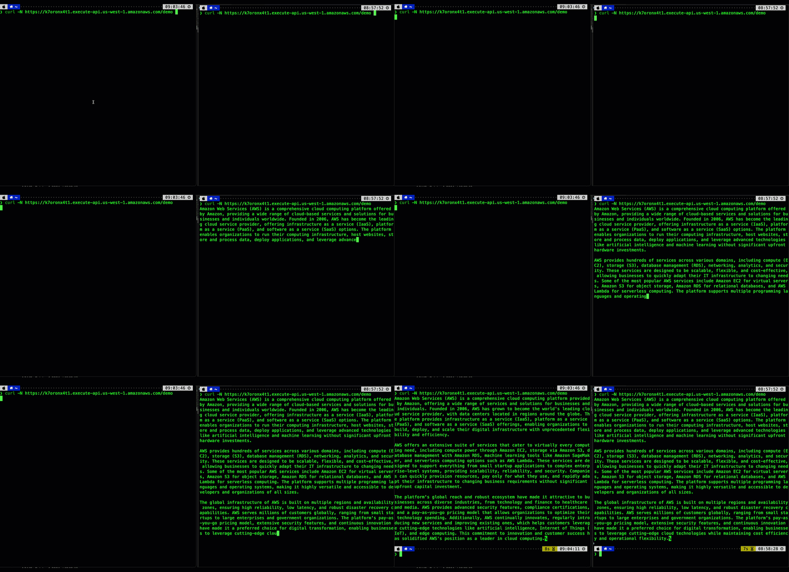
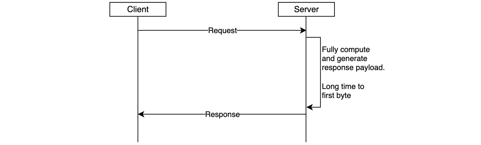
Amazon OpenSearch Serverless monitoring: A CloudWatch setup guide

Post Syndicated from Urmila Iyer original https://aws.amazon.com/blogs/big-data/amazon-opensearch-serverless-monitoring-a-cloudwatch-setup-guide/

Amazon OpenSearch Serverless simplifies the deployment and management of OpenSearch workloads by automatically scaling based on your usage patterns. The service considers key metrics such as shard utilization, storage consumption, and CPU usage while maintaining millisecond-level response times, with the simplicity of a serverless environment.

While OpenSearch Serverless handles scaling automatically, implementing robust monitoring remains crucial for understanding usage patterns, optimizing costs, helping to ensure performance, and maintaining reliability. Proactive monitoring helps organizations detect critical issues with the applications or infrastructure in real time and identify root causes quickly.
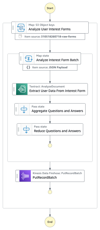
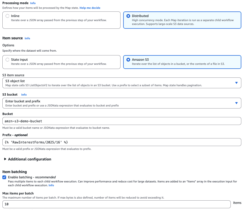
This post is part of our Amazon OpenSearch service monitoring series, focusing on OpenSearch Serverless workloads and deployments. In this post, we explore commonly used Amazon CloudWatch metrics and alarms for OpenSearch Serverless, walking through the process of selecting relevant metrics, setting appropriate thresholds, and configuring alerts. This guide will provide you with a comprehensive monitoring strategy that complements the serverless nature of your OpenSearch deployment while maintaining full operational visibility.

Key benefits of CloudWatch monitoring for OpenSearch Serverless

Implementing CloudWatch monitoring for your OpenSearch Serverless collections offers several key advantages:

  • Near real-time performance monitoring – CloudWatch provides near real-time monitoring, enabling you to track your OpenSearch Serverless collections’ performance as they operate. This immediate visibility allows for swift detection of anomalies or performance issues, enabling prompt response to potential problems.
  • Efficient error diagnosis – You can quickly identify and address common errors without extensive log analysis. For instance, by monitoring ingestion request errors, you can preemptively mitigate bulk indexing request failures.
  • Proactive alerting system – Use the CloudWatch alarm functionality in conjunction with Amazon Simple Notification Service (SNS) to set up custom alerts. By defining specific thresholds for critical metrics, you can receive instant notifications through email or SMS when your OpenSearch Serverless collections approach or exceed these limits.
  • Comprehensive historical analysis – The data retention capabilities of CloudWatch allow for in-depth historical analysis. This helps you to identify long-term performance trends, recognize recurring patterns in resource utilization and optimize workload distribution based on historical insights.

Solution overview

Understanding which metrics to monitor in OpenSearch Serverless helps optimize your system’s performance and reliability. This guide explains the key metrics to monitor, their significance, how to determine appropriate thresholds, and the step-by-step process for setting up alarms. Understanding these fundamentals will help you establish effective monitoring for your OpenSearch Serverless collections and help maintain optimal performance and reliability.

Prerequisites

Before getting started, you must have the following prerequisites:

CloudWatch metrics and recommended alarms for OpenSearch Serverless

The following table summarizes key CloudWatch metrics for OpenSearch Serverless, including recommended alarm thresholds, metric descriptions, and applicable workload types.

Alarm Metric Level Metric Description Alarm Description Use case
IndexingOCU maximum is >= 10 for 5 minutes, three consecutive times Account Level

Serverless compute capacity is measured in OpenSearch Compute Units (OCUs). Each OCU is a combination of 6 GiB of memory and corresponding virtual CPU (vCPU), in addition to data transfer to Amazon Simple Storage Service (Amazon S3).

The IndexingOCU metric reports the number of OCUs used for data ingestion across all collections.

This alarm will alert you when Indexing OCUs scale upto / beyond 10 for more than 15 minutes. Monitor and Optimize Costs
SearchOCU maximum is >= 10 for 5 minutes, three consecutive times Account Level

Serverless compute capacity is measured in OCUs. Each OCU is a combination of 6 GiB of memory and corresponding virtual CPU (vCPU), in addition to data transfer to Amazon S3.

The SearchOCU metric reports the number of OCUs used to search collection data across all collections.

This alarm will alert you when Search OCUs scale upto / beyond 10 for more than 15 minutes. Monitor and Optimize Costs
IngestionRequestLatency maximum is >= 3 secs for 1 minutes, five consecutive times. Collection Level The IngestionRequestLatency metric reports the latency, in seconds, for bulk write operations to a collection. This alarm monitors the maximum latency of bulk write operations to a collection. It triggers when the maximum IngestionRequestLatency exceeds 3 seconds for five consecutive 1-minute intervals (for a total of 5 minutes). This indicates a sustained performance degradation in data ingestion operations, which could impact application performance and data availability. This metric might be crucial to monitor for log-based workloads, where indexing time is critical.
SearchRequestLatency maximum is >= 2 secs for 1 minutes, five consecutive times. Collection Level The SearchRequestLatency metric reports the latency, in seconds, that it takes to complete a search operation against a collection. This alarm monitors the maximum latency of search operations against a collection. It triggers when the maximum SearchRequestLatency exceeds 2 seconds for five consecutive 1-minute intervals (for a total of 5 minutes). Consistently high search latency indicates performance issues that could degrade user experience and application responsiveness. This metric might be crucial to monitor for vector and search-based workloads, where search time is critical.
IngestionRequestErrors sum is >= 100 errors for 1 minute, five consecutive times Collection Level The IngestionRequestErrors metric reports the total number of bulk indexing request errors to a collection. OpenSearch Serverless emits this metric when there are bulk indexing request failures, such as an authentication or availability issue. This alarm monitors the total count of failed bulk indexing operations to a collection. It triggers when the number of IngestionRequestErrors equals or exceeds 100 errors for five consecutive 1-minute intervals (for a total of 5 minutes). Persistent ingestion errors indicate systemic issues that could lead to data loss or inconsistency.
SearchRequestErrors sum is >= 50 errors for 1 minute, five consecutive times Collection Level The SearchRequestErrors metric reports the total number of query errors per minute for a collection. This alarm monitors the total count of failed search query operations in a collection. It triggers when the number of SearchRequestErrors equals or exceeds 50 errors for five consecutive 1-minute intervals (for a total of 5 minutes). Persistent search errors indicate potential issues that could impact application functionality and user experience.
ActiveCollection minimum is 0 for 1 minutes, three consecutive times. Collection Level This metric indicates whether a collection is active. A value of 1 means that the collection is in an ACTIVE state. This value is emitted upon successful creation of a collection and remains 1 until you delete the collection. The metric can’t have a value of 0. The alarm triggers when the metric is missing for three consecutive 1-minute intervals (for a total of 3 minutes). Because an active collection always emits a value of 1, missing data indicates the collection has been deleted or is experiencing serious issues.
Note: Make sure to setup the CloudWatch alarm so that it will treat missing data as breaching.
Monitor Availability of Collection

The specific threshold values mentioned are examples. However, you may need to adjust these thresholds based on the unique requirements and SLAs of your own applications and workloads running on OpenSearch Serverless.

To decide when to raise the global OCU limits, you should regularly review the IndexingOCU and SearchOCU metrics at the account level. If you notice the metrics consistently approaching the set threshold, it’s a good indication that you should consider increasing the overall account limits to accommodate your growing usage.

Additionally, monitor the collection-level metrics like IngestionRequestLatency and SearchRequestLatency. If you notice certain collections have consistently high latency, it might be a sign that the OCU allocation for those specific collections is insufficient. In such cases, you could consider increasing the OCU limits for those high-usage collections, rather than raising the global account limits.

By closely monitoring both the account-level and collection-level metrics, you can make informed decisions about when and how to adjust your OCU limits to maintain optimal performance and cost efficiency for your OpenSearch Serverless deployment.

Steps to create a CloudWatch alarm

CloudWatch Alarms can be created using any of the following methods:

Detailed steps and a / sample code snippet for each method are provided in the following sections.

Using the console

The AWS Management Console provides a user-friendly, visual interface for creating CloudWatch alarms. Follow these step-by-step instructions to set up your alarm through the console.

  1. Navigate to the CloudWatch console
  2. In the navigation pane, choose Alarms and then, All alarms.
  3. Choose Create alarm.

Create an alarm

  1. Choose Select Metric.
  2. Select the namespace AOSS 

Choose CloudWatch Namespace

  1. To setup alerting on IndexingOCU across all collections, navigate to ClientId and select the metric.
  2. Under Conditions:
    1. For Statistic: Select Maximum.
    2. For Period: Select 5 minutes.
    3. For Threshold type: Choose Static and Greater.

Specify metric and conditions

  1. Choose Next. Under Notification, select an SNS topic to notify when the alarm is in ALARM state, OK state, or INSUFFICIENT_DATA state.

Configure Actions

  1. When finished, choose Next. Enter a name and description for the alarm. The name must contain only UTF-8 characters, and can’t contain ASCII control characters. The description can include markdown formatting, which is displayed only in the alarm Details tab in the CloudWatch console. The markdown can be useful to add links to runbooks or other internal resources. Then choose Next.
  2. Under Preview and create, confirm that the information and conditions are what you want, then choose Create alarm.

For detailed documentation, refer to Create a CloudWatch alarm based on a static threshold.

Using the AWS CLI

For those who prefer command-line interfaces or need to automate alarm creation, the AWS CLI offers an efficient alternative. This section demonstrates how to create a CloudWatch alarm using a single CLI command.

To set up a CloudWatch alarm using the AWS CLI, you can use the put-metric-alarm command. The following example demonstrates how to create an alarm that sends an Amazon SNS email when the IndexingOCU exceeds 2 for 15 minutes at the account level. Replace [region] and [account-id] with your AWS Region and account ID.

aws cloudwatch put-metric-alarm \
--alarm-description '# IndexingOCU scaling out' \
--actions-enabled \
--alarm-actions 'arn:aws:sns:[region]:[account-id]:SecurityHubRecurringSummary' \
--metric-name 'IndexingOCU' \
--namespace 'AWS/AOSS' \
--statistic 'Maximum' \
--dimensions '[{"Name":"ClientId","Value":"[account-id]"}]' \
--period 300 \
--evaluation-periods 3 \
--datapoints-to-alarm 3 \
--threshold 2 \
--comparison-operator 'GreaterThanThreshold' \
--treat-missing-data 'ignore'

CloudFormation JSON

Infrastructure as Code (IaC) enables version-controlled, repeatable deployments. This JSON template shows how to define a CloudWatch alarm using AWS CloudFormation, suitable for those who prefer JSON syntax for their IaC implementations.

Replace [region] and [account-id] with your AWS Region and account ID.

{
    "Type": "AWS::CloudWatch::Alarm",
    "Properties": {
        "AlarmDescription": "# IndexingOCU scaling out",
        "ActionsEnabled": true,
        "OKActions": [],
        "AlarmActions": [
            "arn:aws:sns:[region]:[account-id]:SecurityHubRecurringSummary"
        ],
        "InsufficientDataActions": [],
        "MetricName": "IndexingOCU",
        "Namespace": "AWS/AOSS",
        "Statistic": "Maximum",
        "Dimensions": [
            {
                "Name": "ClientId",
                "Value": "[account-id]"
            }
        ],
        "Period": 300,
        "EvaluationPeriods": 3,
        "DatapointsToAlarm": 3,
        "Threshold": 2,
        "ComparisonOperator": "GreaterThanThreshold",
        "TreatMissingData": "ignore"
    }
}

CloudFormation YAML

For teams that prefer YAML’s more readable format, this section provides the equivalent CloudFormation template in YAML. The template creates the same CloudWatch alarm with identical configurations as the JSON version.

Replace [region] and [account-id] with your AWS Region and account ID.

Type: AWS::CloudWatch::Alarm
Properties:
    AlarmDescription: "# IndexingOCU scaling out"
    ActionsEnabled: true
    OKActions: []
    AlarmActions:
        - arn:aws:sns:[region]:[account-id]:SecurityHubRecurringSummary
    InsufficientDataActions: []
    MetricName: IndexingOCU
    Namespace: AWS/AOSS
    Statistic: Maximum
    Dimensions:
        - Name: ClientId
          Value: "[account-id]"
    Period: 300
    EvaluationPeriods: 3
    DatapointsToAlarm: 3
    Threshold: 2
    ComparisonOperator: GreaterThanThreshold
    TreatMissingData: ignore

CloudWatch dashboards

You can use Amazon CloudWatch dashboards to monitor multiple resources in a unified view. For example, the following dashboard provides a consolidated view of OpenSearch Serverless OCU usage, helping you track and manage costs.

View dashboards

Clean up

To avoid incurring unintended future charges, delete the following resources that were created as part of solution walk-through of this post:

  • CloudWatch alarms
  • CloudFormation stacks
  • SNS topics

Conclusion

Effective monitoring helps maintain optimal performance and reliability of your OpenSearch Serverless collections. By implementing the CloudWatch alarms and monitoring strategies outlined in this post, you can work towards proactively identifying and responding to performance issues before they impact your applications, optimize costs by tracking OCU usage patterns, support high availability objectives by monitoring collection health and error rates, and help maintain consistent performance through latency monitoring. Remember that the thresholds suggested in this guide serve as a starting point, you should adjust them based on your specific use cases, performance requirements, and budget constraints. Regular review and refinement of these alarms will help you maintain an efficient and cost-effective OpenSearch Serverless deployment.

Related links

Monitoring Amazon OpenSearch Serverless

Create a CloudWatch alarm based on a static threshold


About the authors

Urmila Iyer

Urmila Iyer

Urmila is a Technical Account Manager at AWS, where she partners with enterprise customers to understand their business objectives and architect solutions that drive meaningful outcomes. With 15 years of experience in IT, including 6 years at AWS, she specializes in data-driven solutions, bringing enthusiasm and expertise to data analytics projects using OpenSearch and real-time analytics platforms.

Parth Shah

Parth Shah

Parth is a Senior Solutions Architect at AWS passionate about solving complex data challenges for strategic customers. As a analytics enthusiast, he helps organizations make sense of their data through innovative cloud solutions, with deep expertise in OpenSearch implementations.
Outside of work, he enjoys spending time with family, exploring different cuisines and playing cricket.

A scalable, elastic database and search solution for 1B+ vectors built on LanceDB and Amazon S3

Post Syndicated from Audra Devoto original https://aws.amazon.com/blogs/architecture/a-scalable-elastic-database-and-search-solution-for-1b-vectors-built-on-lancedb-and-amazon-s3/

This post was co-authored with Owen Janson, Audra Devoto, and Christopher Brown of Metagenomi.

From CRISPR gene editing to industrial biocatalysis, enzymes power some of the most transformative technologies in healthcare, energy, and manufacturing. But discovering novel enzymes that can transform an industry — such as Cas9 for genome engineering — requires sifting through the billions of diverse enzymes encoded by organisms spanning the tree of life. Advances in DNA sequencing and metagenomics have enabled the growth of vast public and proprietary databases containing known protein sequences, but scanning through these collections to identify high value candidates is fundamentally a big data problem as well as a biological one.

At Metagenomi, we’re developing potentially curative therapeutics by using our extensive metagenomics database (MGXdb) to build a toolbox of novel gene editing systems. In this post, we highlight how Metagenomi is tackling the challenge of enzyme discovery at the billion protein scale by using the scalable infrastructure of Amazon Web Services (AWS) to build a high-performance protein database and search solution based on embeddings. By embedding every protein in our large proprietary database into a vector space, making the data accessible using LanceDB built on Amazon Simple Storage Service (Amazon S3), and accessed with AWS Lambda, we were able to transform enzyme discovery into a nearest neighbor search problem and rapidly access previously unexplored discovery space.

Solution overview

At the core of our solution is LanceDB. LanceDB is an open source vector database that enables rapid approximate nearest neighbor (ANN) searches on indexed vectors. LanceDB is particularly well suited for a serverless stack because it’s entirely file-based and is also compatible with Amazon S3 storage. As a result, we can store our database of embedded protein sequences on relatively low-cost Amazon S3, rather than a persistent disk storage such as Amazon Elastic Block Store (Amazon EBS). Instead of constantly running servers, all that is needed to rapidly query the database on-demand is a Lambda function that uses LanceDB to find nearest neighbors directly from the data on S3.

To overcome the challenge of ingesting and querying billions of vector embeddings representing Metagenomi’s large protein database, we devised a method for splitting the database into equal sized parts (folders) stored for low cost on Amazon S3 that can be indexed in parallel and searched with a map-reduce approach using Lambda. The following diagram illustrates this architecture.

AWS architecture showing protein vector processing workflow with ECR, Lambda, and LanceDB

The process follows four steps:

  1. Data vectorization
  2. Data bucketing
  3. Indexing and ingesting data
  4. Querying the database

Data vectorization

To make use of LanceDB’s fast ANN search capabilities, the data must be in vector form. Our metagenomics database consists of billions of proteins, each a string of amino acids. To convert each protein into a vector that captures biologically meaningful information, we run them through a protein language model (pLM), capturing the model’s hidden layers as a vector representation of that protein. Many pLMs can be used to generate protein embeddings, depending on the desired biological information and computational requirements. Here, we use the AMPLIFY_350M model, a transformer encoder model that is fast enough to scale to our entire protein database. We perform a mean-pool of the final hidden layer of the model to produce a 960-dimension vector for each protein. These vectors and their respective unique protein IDs are then stored in HDF5 files.

Data bucketing

To turn our protein vectors into a searchable database, we use LanceDB to build an index suitable for quickly finding ANNs to a query. However, indexing can take a long time and is difficult to distribute across nodes. To speed up indexing, we first divide our data into roughly evenly sized buckets. We then assign each of our embedding HDF5 files to buckets of size roughly equal to 200 million total vectors using a best-fit bin packing algorithm. The exact size packing method used to bucket data depends on the number and dimension of the vectors, as well as their format. Each bucket is ingested into a separate table that will separately reside in a single LanceDB database object store on Amazon S3.

S3 bucket structure showing LanceDB database organization with vector buckets

By bucketing our data, we can produce several smaller databases that can be indexed on separate nodes in a much shorter amount of time. We can also add more data to our database incrementally as a new bucket, instead of reindexing all the existing data.

Ingesting and indexing bucketed data

After the vectorized data has been assigned to a bucket, it’s time to turn it into a LanceDB table and index it to enable fast ANN querying. The details on how to convert your specific data into a LanceDB table can be found in the LanceDB documentation. For each of our buckets of approximately 200 million vectors, we create a LanceDB table with an IVF-PQ index on the cosine distance. For indexing, we use several partitions equal to the square root of the number of inserted rows, and several sub vectors equal to the number of dimensions of our vectors divided by 16.

To make things smoother to query, we name each table after the bucket from which it was created and upload them to a single S3 directory such that their file structure indicates a single LanceDB database with multiple tables.

The following code snippet provides an example of how you might ingest vectors from an HDF5 file containing id and embedding columns into a LanceDB database and index for fast ANN searches based on cosine distance. The only requirements for running this snippet are python >= 3.9, as well as the lancedb, pyarrow, and h5py packages. It should be noted that this snippet was tested and developed using lancedb version 0.21.1 using the asynchronous LanceDB API.

from typing import List, Iterable
from itertools import islice
from math import sqrt
import pyarrow as pa
import datetime
import asyncio
import lancedb
import h5py

def batched(iterable: Iterable, n: int) -> Iterable[List]:
    """Yield batches of n items from iterable."""
    while batch := list(islice(iterable, n)):
        yield batch

async def vectors_to_db(
    vectors: str,
    db: str,
    table_name: str,
    vector_dim: int,
    ingestion_batch_size: int,
) -> int:
    """Ingest and index vectors from an HDF5 file into a LanceDB table.
    Args:
        vectors (str): An HDF5 file containing protein IDs and their
            960-dimension vector representations.
        db (str): Path to the LanceDB database.
        table_name (str): Name of the table to create.
        vector_dim (int): Dimension of the vectors.
    """
    # create db and table
    custom_schema = pa.schema(
        [
            pa.field("embedding", pa.list_(pa.float32(), vector_dim)),
            pa.field("id", pa.string()),
        ]
    )

    # count the total number of rows as they are added to the table
    total_rows = 0

    # open a connection to the new database and create a table
    with await lancedb.connect_async(db) as db_connection:
        with await db_connection.create_table(
            table_name, schema=custom_schema
        ) as table_connection:
            # open vectors file
            with h5py.File(vectors, "r") as vectors_handle:
                # create a generator over the rows
                rows = (
                    {"embedding": e, "id": i}
                    for e, i in zip(
                        vectors_handle["embedding"],
                        vectors_handle["id"],
                    )
                )

                # insert rows in batches to avoid memory issues
                for batch in batched(rows, ingestion_batch_size):
                    total_rows += len(batch)
                    await table_connection.add(batch)

            # optimize the table and remove old data
            await table_connection.optimize(
                cleanup_older_than=datetime.timedelta(days=0)
            )

            # configure the index for the table
            index_config = lancedb.index.IvfPq(
                distance_type="cosine",
                num_partitions=int(sqrt(total_rows)),
                num_sub_vectors=int(
                    vector_dim / 16
                ),
            )

            # index the table
            await table_connection.create_index(
                "embedding", config=index_config
            )

# ingest and index your data
asyncio.run(
    vectors_to_db(
        vectors="./my_vectors.h5",
        db="./test_db",
        table_name="bucket1",
        vector_dim=960,
        ingestion_batch_size=50000
    )
)

The task of vectorizing, ingesting, indexing each bucket could be parallelized over multiple AWS Batch jobs or run on a single Amazon Elastic Compute Cloud (Amazon EC2) instance.

Querying the database

After the data has been bucketed and ingested into a LanceDB database on Amazon S3, we need a way to query it. Because LanceDB can be queried directly from Amazon S3 using the LanceDB Python API, we can use Lambda functions to take a user-provided query vector and search for ANNs, then return the data to the user. However, because our data has been bucketed across several tables in the database, we need to search for nearest neighbors in each bucket and aggregate the results before passing them back to the user.

We implement the query workflow as an AWS Step Functions state machine that manages a query process for each bucket as Lambda processes, as well as a single Lambda process at the end that aggregates the data and writes the resulting ANNs to a .csv file on Amazon S3. However, this could also be implemented as a series of AWS Batch processes or even run locally. The following snippet shows how a process assigned to one bucket could run an ANN query against one of the database’s buckets, requiring only pandas and lancedb to run on python >= 3.9. As detailed before in the ingestion section, we use the asynchronous LanceDB API and lancedb package version 0.21.1.

from typing import List, Iterable
import asyncio
import lancedb
import pandas
import random

async def run_query_async(
    lancedb_s3_uri: str,
    table_name: str,
    q_vec: List[float],
    k: int,
    vec_col: str,
    n_probes: int,
    refine_factor: int,
) -> pandas.DataFrame:
    """Run a query on a LanceDB table.
    Args:
        lancedb_s3_uri (str): S3 URI of the LanceDB database.
        table_name (str): Name of the table to query.
        q_vec (List[float]): Query vector.
        k (int): Number of nearest neighbors to return.
        vec_col (str): Column name of the vector column.
        n_probes (int): Number of probes to use for the query.
        refine_factor (int): Refine factor for the query.
    Returns:
        pandas.DataFrame: DataFrame containing the approximate nearest
        neighbors to the query vector.
    """
    # open a connection to the database and table
    with await lancedb.connect_async(
        lancedb_s3_uri, storage_options={"timeout": "120s"}
    ) as db_connection:
        with await db_connection.open_table(table_name) as table_connection:
            # query the approximate nearest neighbors to the query vector
            df = (
                await table_connection.query()
                .nearest_to(q_vec)
                .column(vec_col)
                .nprobes(n_probes)
                .refine_factor(refine_factor)
                .limit(k)
                .distance_type("cosine")
                .to_pandas()
            )

    return df

# query the example bucket we produced in the last section
bucket1_df = asyncio.run(
    snippets.run_query_async(
        lancedb_s3_uri="s3://mg-analysis/owen/20250415_lancedb_snippet_testing/test_db/",
        table_name="bucket1",
        q_vec=[random.random() for _ in range(960)],
        k=3,
        vec_col="embedding",
        n_probes=1,
        refine_factor=1,
    )
)

The preceding query will return a panda DataFrame of the following structure:

embedding id _distance
[-5.124435, 4.242000, …] id_1 0.000000
[-5.783999, 4.340500, …] id_2 0.001000
[-6.932943, 3.394850, …] id_3 0.04020

Where the embedding column contains the vector representations of the nearest neighbors, the id column their IDs, and the _distance column their cosine distances to the queried vector.

After each bucket has been independently queried across nodes and each has returned a nearest neighbors DataFrame, the results must be merged and subset to return the user. The following snippet shows how you might do this.

def aggregate_nearest_neighbors(
    dfs: List[pandas.DataFrame], k: int
):
    """Aggregate the nearest neighbors for each query vector.
    Args:
        dfs (List[pandas.DataFrame]): A list of DataFrames containing the
            nearest neighbors queried from each bucket.
        k (int): The number of nearest neighbors to aggregate.
    Returns:
        pd.DataFrame: A DataFrame with the aggregated nearest neighbors.
    """
    # concatenate the DataFrames and get the top k nearest neighbors
    return (
        pandas.concat(dfs, ignore_index=True)
        .sort_values(by=["_distance"], ascending=True)
        .reset_index(drop=True)
        .head(k)
    )

# add the dataframes from querying each bucket to a list
dfs = [bucket1_df, bucket2_df, bucket3_df, bucket4_df, bucket_5]

# aggregate the nearest neighbors across all buckets
nearest_neighbors_all_buckets_df = aggregate_nearest_neighbors(dfs, 5)

Optimizing for large batches of queries

Though querying a LanceDB database directly from its S3 object store on Lambda works well for querying the ANNs of one or a few query vectors, some use cases might require querying thousands or even millions of vectors.

One solution we’ve found that scales well to large batches of queries is to modify the preceding query implementation such that it first downloads one of the database buckets to local storage, then queries it locally using the LanceDB API. Because database buckets can have a large storage footprint, this implementation is better suited for AWS Batch jobs than Lambda, and we recommend using optimized instance storage (for example, i4i instances) rather than EBS volumes. After all query Batch jobs finish, a final job can aggregate their results before returning to the user. Orchestration of parallel query jobs and the aggregation job can be done with Nextflow. Though this implementation will have significantly more overhead and latency from downloading the buckets to disk, it can handle larger batches of queries more efficiently and still requires no continuously running server-based database.

Benchmarking results

Indexing strategies and database split sizes depend on your personal need for performance. Consider the following general optimization guidance when customizing to your use case.

An example database created by Metagenomi consisted of 3.5 billion vector embeddings produced by AMPLIFY, of dimension 960. Ingesting and indexing these 3.5B vector embeddings in split sizes of 200M vectors on i4i.8xlarge instances took 108 total compute hours. Because this solution is serverless and can be queried directly from its S3 object store, the only fixed cost of this database is its storage footprint on Amazon S3 (for an indexed database of 3.5B vectors, this is approximately 12.9 TB). Lambda queries can be an exceptionally low-cost querying solution, with many queries costing fractions of a cent.

In general, larger database splits will be more cost effective to query but will result in longer runtimes and longer indexing times. We recommend scaling up database split sizes to the maximum size that results in an acceptable query return time for a single split while also considering limits of parallelization such as maximum concurrent Lambda functions running. Metagenomi identified database splits of 200M vectors each to yield an optimal trade-off in cost and runtime for both small and large queries. We recommend ingesting and indexing on storage-optimized instances, such as those in the i4i family, for optimal performance and cost savings. If querying is to be done on an instance using a disk-based database (as opposed to Lambda and Amazon S3), we also recommend using storage-optimized instances for queries. We found the Lambda implementation could quickly handle single queries requesting up to 50,000 ANNs, or multi queries of up to 100 sequences with fewer than 5 ANNs. Runtime increases linearly with the number of ANNs requested, as shown in the following graph.

Line graph showing query runtime increasing with number of nearest neighbors

Conclusion

In this post, we showed how Metagenomi was able to store and query billions of protein embeddings at low cost using LanceDB implemented with Amazon S3 and AWS Lambda. This work expands on Metagenomi’s patient-driven mission to create curative genetic medicines by accelerating our discovery and engineering platform. Having quick access to the ANN embedding space of a query protein in seconds has enabled the integration of rapid search methods in our extensive analysis pipelines, accelerated the discovery of several diverse and novel enzyme families, and enabled protein engineering efforts by providing scientists with methods to generate and search embeddings on the fly. As Metagenomi continues to rapidly scale protein and DNA databases, horizontal scaling enabled by database splits that can be indexed and searched in parallel facilitates an embedding database solution that scales to future needs.

The solution outlined in this post focuses on vectors produced by a protein large language model (LLM) but can be applied to other vectorized datasets. To learn more about LanceDB integrated with Amazon S3, refer to the LanceDB documentation.

References

  1. Fournier, Quentin, et al. “Protein language models: is scaling necessary?.” bioRxiv (2024): 2024-09.

About the authors

A Lookback at Workers Launchpad and a Warm Welcome to Cohort #6

Post Syndicated from Christopher Rotas original https://blog.cloudflare.com/workers-launchpad-006/

Imagine you have an idea for an AI application that you’re really excited about — but the cost of GPU time and complex infrastructure stops you in your tracks before you even write a line of code. This is the problem founders everywhere face: balancing high infrastructure costs with the need to innovate and scale quickly.

Our startup programs remove those barriers, so founders can focus on what matters the most: building products, finding customers, and growing a business. Cloudflare for Startups launched in 2018 to provide enterprise-level application security and performance services to growing startups. As we built out our Developer Platform, we pivoted last year to offer founders up to $250,000 in cloud credits to build on our Developer Platform for up to one year.

During Birthday Week 2022, we announced our Cloudflare Workers Launchpad Program with an initial $1.25 billion in potential funding for startups building on Cloudflare Workers, made possible through partnerships with 26 leading venture capital (VC) firms. Within months, we expanded VC-backed funding to $2 billion.

Since 2022, we’ve welcomed 145 startups from 23 countries. These startups are solving problems across verticals such as AI and machine learning, developer tools, 3D design, cloud infrastructure, data tools, ad tech, media, logistics, finance, and other industries. We’re especially proud of the female founder representation in recent cohorts — with nearly a third of companies in Cohort #5 run by a female founder. 

Participants engaged in bootcamp sessions with Cloudflare leadership and product teams, covering key topics like product pricing and scaling sales. Startups received hands-on design support from our Solutions Architecture team, empowering these builders to build and scale their full-stack applications on the Cloudflare network. We facilitate countless introductions across the VC network, and are happy to see funding and M&A activity as these startups scale. Cloudflare also identified direct opportunities and acquired Nefeli Networks (Cohort #2) and Outerbase (Cohort #4).

Check out what Launchpad alumni have to say about their experience in the program:

Langbase (Cohort #3)
Ship hyper-personalized AI apps to any LLM, any data, any developer in seconds


“For Langbase, the best part about Workers Launchpad was the incredible support from Cloudflare’s internal teams. It wasn’t just about access to infrastructure; it was the hands-on migration help, rapid feedback loops, and genuine partnership from engineers, product folks, and the broader Cloudflare community. That human support empowered us to iterate faster, solve hard problems, and truly feel like we were building something impactful together. 

Langbase has quickly become one of the most powerful serverless AI clouds for building and deploying AI agents. We process 700 TB of agent memory and 1.2 billion AI agent runs a month. Langbase is an agent lab, and we’ve also launched a coding agent called Command.new, an “agent of agents” that can take your prompts and turn them into production-ready agents by provisioning infrastructure and writing the agent’s code in TypeScript.

My advice for anyone joining future Workers Launchpad cohorts is to use every resource offered. Engage deeply with the Cloudflare teams, ask for feedback early and often, and be open to sharing your challenges and wins, especially in the Discord community, which is super helpful. Cloudflare listens closely to participant feedback and genuinely wants to help startups succeed. Treat it as a two-way conversation and a collaborative growth opportunity. This mindset is what unlocks the real power of the program.”

-Ahmad Awais, Founder & CEO of Langbase

Sherpo.io (Cohort #4)
AI-first no-code platform to build and sell digital content


“Since joining Cohort #4, we’ve exited closed beta and expanded our product suite for content creators. Today, more than 3,000 creators worldwide power their digital product stores with Sherpo, while we continue building and scaling.

We learned as much from fellow startups as from Cloudflare during office hours and sessions, and we got to meet incredible people along the way, including Cloudflare’s CSO, Stephanie Cohen.

For anyone joining, attend every session, listen closely, and ask questions—they’re incredibly valuable. Building on Workers has given us a real advantage, and the team’s pace of innovation only compounds it.”

-Giacomo Di Pinto, Co-Founder & CEO of Sherpo.io

Tightknit AI (Cohort #4)
Embedded community engagement platform built for SaaS


“Beyond the cloud credits that Launchpad provided us to play with every Cloudflare product, the most important aspect of the program we found was our ability to access (and even contribute) to the product roadmap. We were able to connect with product managers and solutions architects that have helped us take our work to the next level.

We’ve recently passed half a million users on the platform and have started to close not just the top Saas businesses in the world, but the top AI companies in the world, including Clay, Gamma, Lindy, beehiiv, Amplitude, Mixpanel, and so many more. The best part is that 100% of application logic is still powered by Cloudflare!

The biggest piece of advice for anyone starting the cohort is attend office hours as much as you can. I can’t tell you how many times we were able to unblock ourselves or even provide real product feedback/bug reports. It was amazing to meet the rest of the cohort and solve problems together that ordinary Cloudflare developers just do not face. So my advice is don’t miss the office hours. They were by far the most valuable part of our experience.”

-Zach Hawtof, Co-Founder & CEO of Tightknit.ai

Render Better (Cohort #4)
Increase e-commerce revenue by automatically optimizing your site speed


“My favorite part of the Launchpad was the community and the leaders who brought us together. The startup and product teams provided expert advice on both business and technical questions through meetings, 1-on-1s, and Discord. Many of them were former founders, so they understood what we were going through and helped us get what we needed. They were crucial in helping us get unstuck, whether we were using obscure Cloudflare features or needed connections to the right people.

I met a lot of great founders who are on the same journey and face the same struggles. Watching them grow was motivating and gave us a morale boost to keep up the fast pace a startup needs.

Since Launchpad, Render Better has scaled to 60 automated site speed optimizations, helping e-commerce sites convert 20% higher powered by Cloudflare Workers. Our growth accelerated after the program, and we’re now optimizing traffic for some of the biggest e-commerce brands like PSD, Polywood, and Self-Portrait. Render Better now processes 5 billion requests each month, made possible by Cloudflare’s global edge network and Workers platform.

Launchpad is truly just that: Cloudflare gives you the resources and attention to help you grow from an idea into something big. Build fast and take as much advantage of the fuel they give you to fly your startup rocket!”

-James Koshigoe, Founder & CEO of Render Better

Launchpad is growing into more than just a program. It is a community of builders and innovators showing what is possible with Cloudflare’s network behind them. With that foundation, we are excited to introduce the next group of entrepreneurs taking the stage in Cohort #6.

Introducing Cohort #6

Before introducing Cohort #6, we want to give one last shout out to Cohort #5. As Launchpad alumni, we cannot wait to see what you achieve. If you didn’t get a chance to check out Cohort #5’s demo day, watch  the recording here.

With that, help us give a warm welcome to the participants of Workers Launchpad Cohort #6:


We’re excited to see what Cohort #6 accomplishes. Follow @CloudflareDev on X and join our Developer Discord to stay updated on their progress. If you’re a startup interested in joining Workers Launchpad, applications for Cohort #7 are now open.

Company

About

Allegory

AI-Powered platform connecting impact to funding

Apgio

Mobile app localization platform with smart AI translations and workflow tooling

Atlas

Building the operating system for restaurants

Bloctave

Configurable rights management platform with instantaneous royalty distribution

Byte

AI code auditor that translates codebases into natural language

Calljmp

Agentic AI backend for apps

Centian

MCP-powered AI Agent middleware for successful and compliant operations

Divinci AI

Release management and quality assurance for custom LLMs

DXOS

An extensible open-core super-app designed to be your team’s brain

Fidsy

AI-native, code-free orchestration platform providing automated data privacy for all AI & Data workflows

Fluentos

Create popups your customers won’t hate

Framebird

Media sharing solution for creatives featuring modern galleries and client review tools

GoPersonal

AI to build, personalize, and manage your ecommerce business

Horizon

Short-form & agentic experiences for apps and websites

Kenobi

Personalizing the Internet with custom web experiences

MonetizationOS

Intelligent decisioning at the edge, for monetising the human and machine web

Natively.dev

Build your dream mobile app using AI, enabling users to take directly to App Stores

Outhire

AI agent automating phone screens without bias

Outsession

Privacy-first AI tools that preserve the therapeutic relationship

Phleid

Direct-to-wallet mobile passes and notifications platform

PlaySafe (By Doge Labs)

Makes voice-chat communities safer by detecting and blocking harassment in real time

Ploton

Help small business businesses grow by building workflows through natural conversation, not complex tools

Project Karna

Multimodal, continuous identity for the post-GenAI enterprise

Schematic

Simplify monetization for GTM teams, allowing them to control pricing, packaging, and entitlements without code changes

SonicLinker

Turn AI-agent visits into revenue

SuiteOp

All-in-one platform to streamline hospitality operations and guest services

SuprSend

Multi-channel notification engine for product and platform teams

Yara AI

Ethical, memory-rich AI for mental health at scale

Zephyr Cloud

Fastest way to go from idea to production

Zero Email

AI native email client that manages your inbox so you don’t have to

Introducing free access to Cloudflare developer features for students

Post Syndicated from Veronica Marin original https://blog.cloudflare.com/workers-for-students/

I can recall countless late nights as a student spent building out ideas that felt like breakthroughs. My own thesis had significant costs associated with the tools and computational resources I needed. The reality for students is that turning ideas into working applications often requires production-grade tools, and having to pay for them can stop a great project before it even starts. We don’t think that cost should stand in the way of building out your ideas.

Cloudflare’s Developer Platform already makes it easy for anyone to go from idea to launch. It gives you all the tools you need in one place to work on that class project, build out your portfolio, and create full-stack applications. We want students to be able to use these tools without worrying about the cost, so starting today, students at least 18 years old in the United States with a verified .edu email can receive 12 months of free access to Cloudflare’s developer features. This is the first step for Cloudflare for Students, and we plan to continue expanding our support for the next generation of builders.


What’s included

12 months of our paid developer features plan at no upfront cost

Eligible student accounts will receive increased usage allotments for our developer features compared to our free plan. That includes Workers, Pages Functions, KV, Containers, Vectorize, Hyperdrive, Durable Objects, Workers Logpush, and Queues. With these, you can build everything from APIs and full-stack apps to data pipelines and websites.

After 12 months, you can easily renew your subscription by upgrading to our Workers Paid plan. If you choose not to, your account will automatically revert to the free plan, and you won’t be charged.

Here’s a look at the increased usage allotments students can receive today. Above those free allotments, our standard usage rates will apply.

Free Plan

Student Accounts (Paid developer features)

Workers

100,000 requests/day

10 million requests/month

+ $.30 per additional million requests

Workers KV

100,000 read operations/day

1,000 write, delete, list operations per day

10 million read operations/month

1 million write, delete, and list operations per month

Hyperdrive

100,000 database queries/day

Unlimited database queries / day

Durable Objects

100,000 requests/day

1 million requests / day

+ $0.15 / per additional million requests

Workers Logs

200,000 log events / day

3 Days of retention

20 million log events / month 

7 Days of retention

+$0.60 per additional million events

Workers Logpush

Not Included

10 million log events / month

+$0.05 per additional million log events

Queues

Not Included

1 million operations/month included 

+$0.40 per additional million operations

Access to a dedicated student developer community

You’ll also have access to a dedicated Discord channel just for students. We want to see what you’re building! This is a place to connect with peers, get support, and share ideas in a community of student developers.

What others have built with Cloudflare’s Developer Platform

Curious about what’s possible with Cloudflare’s developer features? Here are some projects from our community:

by Daniel Foldi


Adventure is a text-based adventure game running on Cloudflare Workers that uses Workers AI to generate the stories with the @cf/google/gemma-3-12b-it model. 

The project’s developer chose Workers AI with the OpenNext adapter because it made deployment simple and handled scaling automatically. It uses the Workers Paid plan mainly to enable Workers Logpush and get access to detailed logs for better monitoring and analysis.

When a new game starts, the server gives the AI a custom prompt to set the scene and explain how the adventure should work. From there, each time the player makes a choice, their story history is sent back to the server, which asks the AI to continue the narrative, allowing the story to evolve dynamically based on the player’s choices.

The code below shows how this logic is implemented:

"use server";
import { getCloudflareContext } from "@opennextjs/cloudflare";

async function prime(env: CloudflareEnv) {
  const id = Math.floor(Math.random() * 1000000);//unique ID for each game run
  const messages = [
    {
      role: "user",
      content:
        `The user is playing a text-based adventure game. Each game is different, this is game ${id}. Your first job is to create a short background story in 3-4 sentences. Scenarios may include interesting locations such as jungles, deserts, caves.
        After the first message, each of your messages will be responses to the user interaction. State three short options (A, B, C). The user responses will be the chosen action. Your responses should end by asking the user about their choice.
        Your message will be shown to the user directly, so avoid "Certainly", "Great", "Let's get started", and other filler content, and avoid bringing up technical details such as "this is game #id".
        The games should have a win condition that is actually feasible given the story, and if the player loses, the message should end with "Try again.".
        `,
    },
  ];
  //Call Workers AI to generate the first response (story intro)
  const { response } = await env.AI.run("@cf/google/gemma-3-12b-it", { messages });

  return [
    ...messages,
    { role: "assistant", content: response }
  ];
}

/**
 * Main server action for the adventure game.
 * If no input yet, it primes the game with the opening story
 * If there is input, it continues the story based on the full history
 * Uses getCloudflareContext from @opennextjs/cloudflare to access env.
 */
export async function adventureAction(input: any[]) {
  let { env } = await getCloudflareContext({ async: true });

  return input.length === 0
  ? await prime(env)
  : [...input,
      { role: "assistant", content: (await env.AI.run("@cf/google/gemma-3-12b-it", { messages: input })).response }
  ];
}

by Matt Cowley


DNS over Discord is a bot that lets you run DNS lookups right inside Discord. Instead of switching to a terminal or online tool, you can use simple slash commands to check records like A, AAAA, MX, TXT, and more.

The developer behind the project chose Cloudflare Workers because it’s a great platform for running small JavaScript apps that handle requests, which made it a good fit for Discord’s slash commands. Since every command translates into a request and the bot sees a lot of traffic, the free tier wasn’t enough, so it now runs on Workers Paid to keep up reliably without hitting request limits.

In this project, the Worker checks if the request is a Discord interaction, and if so, it sends it to the right command (e.g., /dig, /multi-dig, etc.), using a handler that calls out to a custom framework for Discord slash commands. If it’s not from Discord, it can also serve routes like the privacy page or terms of service.

Here’s what that looks like in code:

export default {
  // Process all requests to the Worker
  fetch: async (request, env, ctx) => {
    try {
      // Include the env in the context we pass to the handler
      ctx.env = env;

      // Check if it's a Discord interaction (or a health check)
      const resp = await handler(request, ctx);
      if (resp) return resp;

      // Otherwise, process the request
      const url = new URL(request.url);

      if (request.method === 'GET' && url.pathname === '/privacy')
        return new textResponse(Privacy);

      if (request.method === 'GET' && url.pathname === '/terms')
        return new textResponse(Terms);

      // Fallback if nothing matches
      return new textResponse(null, { status: 404 });
    } catch (err) {
      // Log any errors
      captureException(err);

      // Re-throw the error
      throw err;
    }
  },
};

by James Ross


placeholders.dev is a service that generates placeholder images, making it easy for developers to prototype and scaffold websites without dealing with hosting or asset management. Users can generate placeholders instantly with a simple URL, such as: https://images.placeholders.dev/350x150

Since placeholders are typically used in early development, speed and consistency matter, and images need to load instantly so the workflow isn’t interrupted. Running on Cloudflare Workers makes the service fast and consistent no matter where developers are.

This project uses the Workers Paid plan because it regularly exceeds the free-tier limits on requests and compute time. The Worker below shows the core of how the service works. When a request comes in, it looks at the URL path (like /300x150) to determine the size of the placeholder, applies some defaults for style, and then returns an SVG image on the fly.

export default {
  async fetch(request: Request, env: Env, ctx: ExecutionContext) {
    try {
      const url = new URL(request.url);
      const cache = caches.default;

      // Handle requests for the placeholder API
      if (url.host === 'images.placeholders.dev' || url.pathname.startsWith('/api')) {
        // Try edge cache first
        const cached = await cache.match(url, { ignoreMethod: true });
        if (cached) return cached;

        // Default placeholder options
        const imageOptions: Options = {
   dataUri: false, // always return an unencoded SVG source
          width: 300,
          height: 150,
          fontFamily: 'sans-serif',
          fontWeight: 'bold',
          bgColor: '#ddd',
          textColor: 'rgba(0,0,0,0.5)',
        };

        // Parse sizes from path (e.g. /350 or /350x150)
        const sizeParts = url.pathname.replace('/api', '').replace('/', '').split('x');
        if (sizeParts[0]) {
          const width = sanitizeNumber(parseInt(sizeParts[0], 10));
          const height = sizeParts[1] ? sanitizeNumber(parseInt(sizeParts[1], 10)) : width;
          imageOptions.width = width;
          imageOptions.height = height;
        }

        // Generate SVG placeholder
        const response = new Response(simpleSvgPlaceholder(imageOptions), {
          headers: { 'content-type': 'image/svg+xml; charset=utf-8' },
        });

        // Cache result
        response.headers.set('Cache-Control', 'public, max-age=' + cacheTtl);
        ctx.waitUntil(cache.put(url, response.clone()));

        return response;
      }

      return new Response('Not Found', { status: 404 });
    } catch (err) {
      console.error(err);
      return new Response('Internal Error', { status: 500 });
    }
  },
};

Check out Built With Workers to see what other developers are building with our developer platform.


How do I get started?

This offering is available to United States students at least 18 years old with a verified .edu billing email address.

Based on when your account was created, you can redeem this offer either by signing up for a free Cloudflare account with your .edu email or by filling out a form to request access for your existing .edu account. Just make sure your verified .edu email address is your billing email address.

New .edu accounts

Existing .edu accounts

Creation Date 

Created on/after September 22, 2025

Created prior to September 22, 2025

How to Redeem

Sign up for a free Cloudflare account, add your credit card and ensure your verified .edu email address is added to your billing details.

Ensure your verified .edu email address is added to your billing details.

Fill out our form and a member of our team will help you get access

Note: in order to receive the credit, your verified .edu email address needs to be your billing email address 

Expanding Cloudflare for Students coverage

While our first offering is primarily for institutions in the US, we’re working on expanding support for our students in other countries and plan to add additional higher education domain names after launch. If you’re at an educational institution outside of the United States, please reach out to us and apply for your educational/academic domain to be added. We’ll let you know as soon as it becomes available in your region. Check our Cloudflare for Students page for updates and keep an eye out for emails if you have an account with a newly supported domain.

Whether you’re gearing up for your first hackathon, launching a side project, or looking to build the next big thing, you can get started today with free access and join a global developer community already building on Cloudflare.

Get started by signing up or requesting access today.


Come build with us: Cloudflare’s new hubs for startups

Post Syndicated from Christopher Rotas original https://blog.cloudflare.com/new-hubs-for-startups/

Cloudflare’s offices bring together builders in some of the world’s most popular technology hubs. We have a long history of using those spaces for one-off events and meet ups over the last fifteen years, but we want to do more. Starting in 2026, we plan to open the doors of our offices routinely to startups and builders from outside of our team who need the space to collaborate, meet new people, or just type away at a keyboard in a new (and beautiful) location.

What are our offices meant to be?

Prior to 2020, we expected essentially every team member of Cloudflare to be present in one of our offices five days a week. That worked well for us and helped facilitate the launch of dozens of technologies as well as a community and culture that defined who we are.

Like every other team on the planet, the COVID pandemic forced us to revisit that approach. We used the time to think about what our offices could be, in a world where not every team member showed up every day of the week. While we decided we would be open to remote and hybrid work, we still felt like some of our best work was done in person together. The goal became building spaces that encouraged team members to be present.

Several hard hats and a few leases later, we’ve created a network of offices around the world designed to evolve with the way people work. These spaces aren’t just places to sit — they’re environments that empower people to do their best work — whether that means quiet focus, creative problem-solving, or lively collaboration. From a library tucked into a quiet zone in our waterfront Lisbon office, to the high-ceilinged collaboration areas in the heart of Austin, each office reflects our belief that great spaces support diverse working styles and help teams thrive together.

Our offices are meant to connect our teams, and we believe that by opening our doors to the wider community, we can foster even more innovation and help new companies collaborate better. Cloudflare has always been a hub for builders, and now we’re making that commitment official by welcoming startups into our physical spaces.

Why make them even more open to the community?

Our spaces have served as hosts to community events since the earliest days of Cloudflare. We have brought together just about every group from hackathons to language meet-ups to university orientation sessions. Cloudflare exists to help build a better Internet and in many cases a better digital environment starts with relationships built in a real life environment.

One of the most common pieces of feedback we have received in the last few years after hosting these events is “I really miss connecting with people like this.” And we hear that most often from small teams in the earliest stages of their journey. In the last few years as the start-ups we support with our platform increasingly begin remote-first and only open dedicated spaces in later stages of their growth.

We know that building a company can be a lonely path. We have helped over the last several years by providing a robust free plan and a comprehensive start-up program, but we think we can do more.

Cloudflare’s network supports a significant percentage of the Internet and, as you would expect, the Internet follows the sun. More people use it during the daytime than at night, meaning our data center utilization peaks in specific times of the day. We take advantage of that pattern to run services that are less latency-sensitive in regions overnight.

Our physical locations follow a similar pattern. Utilization resembles a bell curve with Tuesdays, Wednesdays, and Thursdays seeing a lot of traffic while Mondays and Fridays tend to be quieter. Like our CPUs at night, we think we can use that excess capacity to help build a better Internet by giving builders a space to congregate and helping our team connect with more of our users.

How will this work?

Beginning in January of 2026, we plan to make our office locations available to a capped number of external visitors as all-day coworking spaces on select days of each week. We will provide a registration process (more on that below) and set some ground rules. To start, we plan to expand this offering to San Francisco, Austin, London, and Lisbon.

When external visitors arrive, they’ll have access to our common spaces to bring together their teams or just get some work done by themselves. No mandatory talks or obligations. Just fantastic working spaces available to use at no cost.

How can you participate?

We will provide more details in the next few weeks, but the general structure will be based on the following steps.

  1. Enroll in the Cloudflare for Startups Program. Bonus if you are a Workers Launchpad participant or alumni.

  2. Sit tight for now. We will email participating Startup Program customers first to participate with a form requesting office access.

  3. Once the form is filled out, a member of our team will reach out after. If you want to get a head start, fill out the form here.

  4. We plan to roll this out on a cohort basis. Once approved and all requirements are met, register your visit (and that of any additional team members) at least three business days prior to the date requested.

  5. Respect our working spaces as you would your own.

What’s next?

We hope to expand to other locations in the future. Want to get to the front of the line? Sign up for our Startup program here today and we will reach out to Startup Program participants before we roll out the program.

Qwen models are now available in Amazon Bedrock

Post Syndicated from Danilo Poccia original https://aws.amazon.com/blogs/aws/qwen-models-are-now-available-in-amazon-bedrock/

Today we are adding Qwen models from Alibaba in Amazon Bedrock. With this launch, Amazon Bedrock continues to expand model choice by adding access to Qwen3 open weight foundation models (FMs) in a full managed, serverless way. This release includes four models: Qwen3-Coder-480B-A35B-Instruct, Qwen3-Coder-30B-A3B-Instruct, Qwen3-235B-A22B-Instruct-2507, and Qwen3-32B (Dense). Together, these models feature both mixture-of-experts (MoE) and dense architectures, providing flexible options for different application requirements.

Amazon Bedrock provides access to industry-leading FMs through a unified API without requiring infrastructure management. You can access models from multiple model providers, integrate models into your applications, and scale usage based on workload requirements. With Amazon Bedrock, customer data is never used to train the underlying models. With the addition of Qwen3 models, Amazon Bedrock offers even more options for use cases like:

  • Code generation and repository analysis with extended context understanding
  • Building agentic workflows that orchestrate multiple tools and APIs for business automation
  • Balancing AI costs and performance using hybrid thinking modes for adaptive reasoning

Qwen3 models in Amazon Bedrock
These four Qwen3 models are now available in Amazon Bedrock, each optimized for different performance and cost requirements:

  • Qwen3-Coder-480B-A35B-Instruct – This is a mixture-of-experts (MoE) model with 480B total parameters and 35B active parameters. It’s optimized for coding and agentic tasks and achieves strong results in benchmarks such as agentic coding, browser use, and tool use. These capabilities make it suitable for repository-scale code analysis and multistep workflow automation.
  • Qwen3-Coder-30B-A3B-Instruct – This is a MoE model with 30B total parameters and 3B active parameters. Specifically optimized for coding tasks and instruction-following scenarios, this model demonstrates strong performance in code generation, analysis, and debugging across multiple programming languages.
  • Qwen3-235B-A22B-Instruct-2507 – This is an instruction-tuned MoE model with 235B total parameters and 22B active parameters. It delivers competitive performance across coding, math, and general reasoning tasks, balancing capability with efficiency.
  • Qwen3-32B (Dense) – This is a dense model with 32B parameters. It is suitable for real-time or resource-constrained environments such as mobile devices and edge computing deployments where consistent performance is critical.

Architectural and functional features in Qwen3
The Qwen3 models introduce several architectural and functional features:

MoE compared with dense architectures – MoE models such as Qwen3-Coder-480B-A35B, Qwen3-Coder-30B-A3B-Instruct, and Qwen3-235B-A22B-Instruct-2507, activate only part of the parameters for each request, providing high performance with efficient inference. The dense Qwen3-32B activates all parameters, offering more consistent and predictable performance.

Agentic capabilities – Qwen3 models can handle multi-step reasoning and structured planning in one model invocation. They can generate outputs that call external tools or APIs when integrated into an agent framework. The models also maintain extended context across long sessions. In addition, they support tool calling to allow standardized communication with external environments.

Hybrid thinking modes – Qwen3 introduces a hybrid approach to problem-solving, which supports two modes: thinking and non-thinking. The thinking mode applies step-by-step reasoning before delivering the final answer. This is ideal for complex problems that require deeper thought. Whereas the non-thinking mode provides fast and near-instant responses for less complex tasks where speed is more important than depth. This helps developers manage performance and cost trade-offs more effectively.

Long-context handling – The Qwen3-Coder models support extended context windows, with up to 256K tokens natively and up to 1 million tokens with extrapolation methods. This allows the model to process entire repositories, large technical documents, or long conversational histories within a single task.

When to use each model
The four Qwen3 models serve distinct use cases. Qwen3-Coder-480B-A35B-Instruct is designed for complex software engineering scenarios. It’s suited for advanced code generation, long-context processing such as repository-level analysis, and integration with external tools. Qwen3-Coder-30B-A3B-Instruct is particularly effective for tasks such as code completion, refactoring, and answering programming-related queries. If you need versatile performance across multiple domains, Qwen3-235B-A22B-Instruct-2507 offers a balance, delivering strong general-purpose reasoning and instruction-following capabilities while leveraging the efficiency advantages of its MoE architecture. Qwen3-32B (Dense) is appropriate for scenarios where consistent performance, low latency, and cost optimization are important.

Getting started with Qwen models in Amazon Bedrock
To begin using Qwen models, in the Amazon Bedrock console, I choose Model Access from the Configure and learn section of the navigation pane. I then navigate to the Qwen models to request access. In the Chat/Text Playground section of the navigation pane, I can quickly test the new Qwen models with my prompts.

To integrate Qwen3 models into my applications, I can use any AWS SDKs. The AWS SDKs include access to the Amazon Bedrock InvokeModel and Converse API. I can also use these model with any agentic framework that supports Amazon Bedrock and deploy the agents using Amazon Bedrock AgentCore. For example, here’s the Python code of a simple agent with tool access built using Strands Agents:

from strands import Agent
from strands_tools import calculator

agent = Agent(
    model="qwen.qwen3-coder-480b-instruct-v1:0",
    tools=[calculator]
)

agent("Tell me the square root of 42 ^ 9")

with open("function.py", 'r') as f:
    my_function_code = f.read()

agent(f"Help me optimize this Python function for better performance:\n\n{my_function_code}")

Now available
Qwen models are available today in the following AWS Regions:

  • Qwen3-Coder-480B-A35B-Instruct is available in the US West (Oregon), Asia Pacific (Mumbai, Tokyo), and Europe (London, Stockholm) Regions.
  • Qwen3-Coder-30B-A3B-Instruct, Qwen3-235B-A22B-Instruct-2507, and Qwen3-32B are available in the US East (N. Virginia), US West (Oregon), Asia Pacific (Mumbai, Tokyo), Europe (Ireland, London, Milan, Stockholm), and South America (São Paulo) Regions.

Check the full Region list for future updates. You can start testing and building immediately without infrastructure setup or capacity planning. To learn more, visit the Qwen in Amazon Bedrock product page and the Amazon Bedrock pricing page.

Try Qwen models on the Amazon Bedrock console now, and offer feedback through AWS re:Post for Amazon Bedrock or your typical AWS Support channels.

Danilo

DeepSeek-V3.1 model now available in Amazon Bedrock

Post Syndicated from Channy Yun (윤석찬) original https://aws.amazon.com/blogs/aws/deepseek-v3-1-now-available-in-amazon-bedrock/

In March, Amazon Web Services (AWS) became the first cloud service provider to deliver DeepSeek-R1 in a serverless way by launching it as a fully managed, generally available model in Amazon Bedrock. Since then, customers have used DeepSeek-R1’s capabilities through Amazon Bedrock to build generative AI applications, benefiting from the Bedrock’s robust guardrails and comprehensive tooling for safe AI deployment.

Today, I am excited to announce DeepSeek-V3.1 is now available as a fully managed foundation model in Amazon Bedrock. DeepSeek-V3.1 is a hybrid open weight model that switches between thinking mode (chain-of-thought reasoning) for detailed step-by-step analysis and non-thinking mode (direct answers) for faster responses.

According to DeepSeek, the thinking mode of DeepSeek-V3.1 achieves comparable answer quality with better results, stronger multi-step reasoning for complex search tasks, and big gains in thinking efficiency compared with DeepSeek-R1-0528.

Benchmarks DeepSeek-V3.1 DeepSeek-R1-0528
Browsecomp 30.0 8.9
Browsecomp_zh 49.2 35.7
HLE 29.8 24.8
xbench-DeepSearch 71.2 55.0
Frames 83.7 82.0
SimpleQA 93.4 92.3
Seal0 42.6 29.7
SWE-bench Verified 66.0 44.6
SWE-bench Multilingual 54.5 30.5
Terminal-Bench 31.3 5.7
(c)
https://api-docs.deepseek.com/news/news250821

DeepSeek-V3.1 model performance in tool usage and agent tasks has significantly improved through post-training optimization compared to previous DeepSeek models. DeepSeek-V3.1 also supports over 100 languages with near-native proficiency, including significantly improved capability in low-resource languages lacking large monolingual or parallel corpora. You can build global applications to deliver enhanced accuracy and reduced hallucinations compared to previous DeepSeek models, while maintaining visibility into its decision-making process.

Here are your key use cases using this model:

  • Code generation – DeepSeek-V3.1 excels in coding tasks with improvements in software engineering benchmarks and code agent capabilities, making it ideal for automated code generation, debugging, and software engineering workflows. It performs well on coding benchmarks while delivering high-quality results efficiently.
  • Agentic AI tools – The model features enhanced tool calling through post-training optimization, making it strong in tool usage and agentic workflows. It supports structured tool calling, code agents, and search agents, positioning it as a solid choice for building autonomous AI systems.
  • Enterprise applications – DeepSeek models are integrated into various chat platforms and productivity tools, enhancing user interactions and supporting customer service workflows. The model’s multilingual capabilities and cultural sensitivity make it suitable for global enterprise applications.

As I mentioned in my previous post, when implementing publicly available models, give careful consideration to data privacy requirements when implementing in your production environments, check for bias in output, and monitor your results in terms of data security, responsible AI, and model evaluation.

You can access the enterprise-grade security features of Amazon Bedrock and implement safeguards customized to your application requirements and responsible AI policies with Amazon Bedrock Guardrails. You can also evaluate and compare models to identify the optimal model for your use cases by using Amazon Bedrock model evaluation tools.

Get started with the DeepSeek-V3.1 model in Amazon Bedrock
If you’re new to using the DeepSeek-V3.1 model, go to the Amazon Bedrock console, choose Model access under Bedrock configurations in the left navigation pane. To access the fully managed DeepSeek-V3.1 model, request access for DeepSeek-V3.1 in the DeepSeek section. You’ll then be granted access to the model in Amazon Bedrock.

Next, to test the DeepSeek-V3.1 model in Amazon Bedrock, choose Chat/Text under Playgrounds in the left menu pane. Then choose Select model in the upper left, and select DeepSeek as the category and DeepSeek-V3.1 as the model. Then choose Apply.

Using the selected DeepSeek-V3.1 model, I run the following prompt example about technical architecture decision.

Outline the high-level architecture for a scalable URL shortener service like bit.ly. Discuss key components like API design, database choice (SQL vs. NoSQL), how the redirect mechanism works, and how you would generate unique short codes.

You can turn the thinking on and off by toggling Model reasoning mode to generate a response’s chain of thought prior to the final conclusion.

You can also access the model using the AWS Command Line Interface (AWS CLI) and AWS SDK. This model supports both the InvokeModel and Converse API. You can check out a broad range of code examples for multiple use cases and a variety of programming languages.

To learn more, visit DeepSeek model inference parameters and responses in the AWS documentation.

Now available
DeepSeek-V3.1 is now available in the US West (Oregon), Asia Pacific (Tokyo), Asia Pacific (Mumbai), Europe (London), and Europe (Stockholm) AWS Regions. Check the full Region list for future updates. To learn more, check out the DeepSeek in Amazon Bedrock product page and the Amazon Bedrock pricing page.

Give the DeepSeek-V3.1 model a try in the Amazon Bedrock console today and send feedback to AWS re:Post for Amazon Bedrock or through your usual AWS Support contacts.

Channy