Post Syndicated from The History Guy: History Deserves to Be Remembered original https://www.youtube.com/watch?v=71FtfKrl-1M
From Backup to Assurance: Monitoring Veeam with Zabbix
Post Syndicated from Michael Kammer original https://blog.zabbix.com/from-backup-to-assurance-monitoring-veeam-with-zabbix/33694/
Your data isn’t truly protected if you don’t know when that protection fails. Today’s organizations depend on backup infrastructure to safeguard critical workloads, yet a single backup failure, dwindling repository capacity, expired license, security incident, or infrastructure issue can quietly undermine that protection. The key isn’t just having backups – it’s knowing, as quickly and reliably as possible, when something has gone wrong.
Simply having a backup solution in place is not enough. IT teams need continuous visibility into health and operational status. That’s where Zabbix and Veeam come together.
With the latest integrations for Zabbix 8.0 and Veeam Backup & Replication v13, organizations can bring Veeam backup monitoring into their broader infrastructure monitoring strategy, gaining centralized visibility, proactive alerting, and a clearer picture of whether their data protection environment is ready when it is needed. Veeam protects your data. Zabbix makes sure you always know when that protection is at risk.
Two ways to monitor your Veeam environment
Zabbix provides integrations for monitoring Veeam environments through two approaches:
- Veeam Backup & Replication by HTTP
- Veeam Backup Enterprise Manager by HTTP
Both approaches extend Zabbix monitoring into the backup environment, helping teams detect operational and security issues before they become business-impacting incidents.
The Veeam Backup & Replication by HTTP integration provides direct monitoring capabilities for Veeam environments and offers administrators detailed visibility into backup operations and the infrastructure that supports them.
The Veeam Backup Enterprise Manager by HTTP integration is an alternative for organizations that use Veeam Backup Enterprise Manager to centrally manage multiple Veeam Backup & Replication deployments. It uses the Enterprise Manager REST API to bring information from multiple deployments into Zabbix.
It’s important to note that Enterprise Manager is an additional Veeam component and requires a separate installation. For organizations that already have Enterprise Manager deployed, its centralized architecture can make it a valuable option for bringing multiple Veeam environments into a single Zabbix monitoring view.
Veeam Backup & Replication by HTTP: Direct visibility into your backup environment
The Veeam Backup & Replication integration focuses on the operational health of the backup infrastructure and the results of backup activities. With Zabbix, administrators can monitor important components and events, including:
- Backup job status and execution results
- Backup sessions and failures
- Backup repositories and available capacity
- Backup proxies and managed servers
- License status and expiration
- Security Analyzer findings
- Malware detection events
- Authentication and security-related events
NOTE: License, Authorization Events, and Security Analyzer Data require the “Backup Administrator” role; without it, these items are not supported.
This means backup monitoring becomes part of the same monitoring workflow used for servers, applications, networks, storage, and other critical infrastructure. Instead of discovering a failed backup when a recovery is already required, teams can receive an alert as soon as the failure occurs.
Veeam Backup Enterprise Manager by HTTP: Centralized observability across deployments
For organizations managing multiple Veeam Backup & Replication deployments, Veeam Backup Enterprise Manager offers another way to centralize backup information. This Zabbix integration communicates with Enterprise Manager through its REST API and provides centralized monitoring and alerting across multiple Veeam Backup & Replication environments. This gives administrators visibility into areas like:
- Backup infrastructure health
- Backup job status
- Repository utilization
- Operational events
- Job run results
- VM protection status
The result is a consolidated view of backup operations from a single Zabbix dashboard. The integration also works without external scripts and uses a Zabbix script item, helping simplify deployment and ongoing maintenance. This means that Enterprise Manager can be especially useful when an organization already operates it as a centralized management layer for multiple Veeam deployments.
Why monitor Veeam with Zabbix?
Veeam is responsible for protecting data. Zabbix adds a monitoring and alerting layer that helps ensure the protection itself remains healthy. This distinction is important!
A backup job can exist without actually providing reliable protection. Repositories can run out of capacity. Backup jobs can fail repeatedly. Infrastructure components can become unavailable. Licenses can approach expiration. Security-related events can require immediate attention.
Without proactive monitoring, these conditions can remain unnoticed until they have serious consequences. By integrating Veeam into Zabbix, organizations can continuously monitor these conditions and incorporate them into their existing operational processes.
A single pane of glass. IT teams often manage complex environments containing physical and virtual servers, cloud services, networks, storage, applications, and backup infrastructure. Bringing Veeam into Zabbix means that backup operations can be monitored alongside the rest of the environment rather than through an isolated monitoring workflow. This provides a single pane of glass for infrastructure and backup operations and gives administrators a more complete picture of overall service health.
Immediate detection of backup failures. A successful backup is one of the most important indicators that data protection is working as expected. Zabbix can alert teams when backup jobs or sessions fail, allowing them to investigate while there is still time to resolve the problem and complete a successful backup. This changes backup monitoring from a reactive process into a proactive one.
Proactive capacity monitoring. Backup repositories require sufficient capacity to continue protecting data. Monitoring repository utilization and available capacity allows administrators to identify trends and potential capacity problems before they cause backup failures. Instead of reacting to a full repository, teams can plan capacity increases or optimize retention policies ahead of time.
Faster troubleshooting. When something goes wrong, knowing that a backup failed is only the first step. Monitoring the surrounding infrastructure and Veeam components in the same platform can provide valuable context. Zabbix can help teams correlate backup-related events with infrastructure conditions, making it easier to identify potential causes and accelerate troubleshooting.
Reduced recovery risk. The real value of a backup becomes apparent when an organization needs to recover data.
A continuously monitored backup environment provides greater confidence that backup jobs complete successfully, repositories have sufficient capacity, and critical components remain operational. Proactive monitoring, therefore, directly reduces recovery risks and improves both business continuity and disaster recovery readiness.
Security-aware monitoring. Modern backup environments are also an important part of an organization’s security strategy.
Monitoring Veeam security-related information, including malware detection events, Security Analyzer findings, and authentication or security-related events, helps teams identify conditions that may require immediate investigation. Combining these signals with the rest of the organization’s monitoring data can provide additional context when responding to potential threats.
Zabbix 8.0 and Veeam Backup & Replication v13: Keeping the integration current
The latest integration updates for Zabbix 8.0 and Veeam Backup & Replication v13 make it easier for organizations running current versions of these platforms to incorporate Veeam into their monitoring strategy. Keeping integrations aligned with current platform versions is important for organizations that want to modernize their infrastructure while maintaining consistent monitoring and alerting.
Whether you’re observing a single Veeam deployment directly through Veeam Backup & Replication or using Enterprise Manager to centralize multiple deployments, the goal is the same – to
make the state of your backup environment visible and actionable.
From backup monitoring to backup assurance
The biggest benefit of monitoring Veeam with Zabbix is not simply having more metrics or dashboards. It’s the peace of mind that comes from knowing that your data is fully protected at all times. After all, a backup system shouldn’t be something that IT teams think about only when they need to restore data. Its health should be continuously visible, and potential problems should generate alerts before they become emergencies.
Together, Veeam and Zabbix provide a proactive approach to backup monitoring. Veeam protects your data, and Zabbix helps you verify that the protection remains healthy. By combining backup monitoring with broader infrastructure observability, organizations can detect failures earlier, respond faster, plan capacity more effectively, and increase confidence in their business continuity and disaster recovery readiness.
For organizations running Veeam, monitoring the backup environment should be an essential part of the protection strategy, because knowing that your backups are working is just as important as having backups in the first place.
Visit Zabbix to find out more about open source observability, and check out Veeam’s website to discover data protection and resilience solutions.
The post From Backup to Assurance: Monitoring Veeam with Zabbix appeared first on Zabbix Blog.
На второ четене: „Горски цар“
Post Syndicated from Стефан Иванов original https://www.toest.bg/na-vtoro-chetene-gorski-tsar/
„Горски цар“ от Мишел Турние

превод от френски Изабела Георгиева, София: изд. „Парадокс“, 2024
Има книги, които човек препрочита, и книги, които препрочитат него. „Горски цар“ на Мишел Турние принадлежи към втория вид. За първи път го прочетох в гимназията, на онази възраст, когато всеки роман е или откровение, или скука, и той се оказа много важен за мен с някаква смущаваща, почти неприлична настойчивост. После, по инерцията на заразата, изчетох всичко останало на Турние на български и на френски – от „Петкан“ до „Метеорите“ и „Златната капка“. Днес възприемам това като един от решаващите етапи в читателското си развитие, врата с надпис, който се разчита едва след като си я затворил зад себе си. Новото издание на „Парадокс“ в превода на Изабела Георгиева е добър повод за второ четене, което по дефиниция е и разследване на първото.
Сюжетът изглежда като биография, сглобена от случайности, и точно в това е капанът. Абел Тифож, собственик на автосервиз на площад „Порт дьо Терн“, пише своите „Опаки записки“ с лявата си ръка след злополука с манивелата. Заглавието е решение на преводачката, което запазва двусмислието на френското sinistre – едновременно ляво и зловещо. Детството му в колежа „Свети Христофор“ е белязано от Нестор, чудовищно развито дете, което го посвещава в тайнописа на знаците. Обвинението в посегателство над момиченцето Мартина го изпраща към съда. Войната от 1939 г. идва като deus ex machina, която го спасява и отнася. Следват гълъбите на Рейн, пленът в Източна Прусия и ловните гори на Роминтен, където Гьоринг царува като карикатурен людоед сред трофеите си. Накрая идва Калтенборн – националполитическа школа за елитни момчета. Там Тифож, облечен в пълната си митологическа униформа, обикаля околните села на кон и събира деца за Райха. Главите се казват „Роминтенският човекоядец“ и „Калтенборнският човекоядец“ и не хитруват.
Сърцевината на романа е понятието фория, носенето. Тифож открива екстаза на тялото, което носи друго тяло.
Около него изгражда цяла теология, опряна на свети Христофор, пренесъл Христос през реката, и на баладата на Гьоте, в която бащата носи сина си през нощта, а Горският цар го отнема. Турние, възпитаник на Башлар и слушател на Леви-Строс, строи символна машина с часовникарска прецизност. Всеки знак има своя обратен образ и благословията се среща със своята злокачествена инверсия. Носенето спасява и поглъща. Роговете на елена са едновременно триумф и огледален фалос. Дори името на героя е шифър. Тифож е замъкът на Жил дьо Ре, спътника на Жана д’Арк и детеубиеца, когото Юисманс описва в „Там долу“ и Жорж Батай го анализира в свое изследване.
Прочетен в контекста на цялото творчество на Турние, романът разкрива и своята генеалогия. В „Петкан“ той обръща Дефо и превръща Робинзон от колонизатор в ученик на дивака. В „Метеорите“ разиграва мита за близнаците като утопия на затвореното тяло. „Горски цар“ е най-тъмният панел в този триптих от пренаписани митове. Тук методът е подложен на най-тежкото изпитание, защото материалът му е историята, която не търпи алегория. Турние го знае и затова подковава фикцията с бележки под линия към Нюрнбергския процес, сякаш документът е призван да удържи мита да не отлети в чиста поезия.
Тук критическото четене трябва да бъде по-внимателно от възхищението. Силата на книгата и нейният проблем са едно и също нещо. Тифож чете света като йероглифи, изписани лично за него, и романът му дава право, защото съдбата наистина му намига.
Читателят е поканен да опознае една херменевтика, която логически съвпада с параноята и естетически съвпада с фашизма.
Сюзан Зонтаг пише своето есе „Очарователният фашизъм“ пет години след романа. Тя описва точно този култ към здравото тяло, ритуала и подчинението като еротика. Турние го показва отвътре, с лупа и без морален коментар и затова е неудобен. Педофилският подтекст се мярка като сянка, достатъчно ясна, за да я видиш, и достатъчно неназована, за да те направи съучастник в мълчанието. Финалът е изкупление с почти католическа хореография. Тифож носи еврейското момче Ефраим през блатото и потъва под тежестта му, докато над него се върти златна шестолъчна звезда. Красиво е, може би прекалено красиво. Символната система се затваря като ковчеже и изкушението да я приемеш като прошка е силно. При първото четене тази звезда ме разплака. При второто ме накара да се запитам кой всъщност е спасен – дали това е детето, героят или авторът.

Паралелите със световната литература се предлагат сами. „Тенекиеният барабан“ на Грас разказва същата епоха през погледа на детето, което отказва да порасне. „Горски цар“ я разказва през погледа на великана, който отказва на детето да порасне. „Доктор Фаустус“ на Томас Ман проследява как германският мит се превръща в катастрофа. Турние стига до същото, но с френска наслада от германския мит.
„Лолита“ на Набоков е най-близкият роднина по техника и отново е с чудовищен разказвач, чиято реторика е по-обаятелна от моралния ни рефлекс.
„Доброжелателните“ на Джонатан Лител, трийсет и шест години по-късно, повтарят жеста с есесовец вместо с френски пленник и показват колко далеч е отишъл Турние пръв. Над всички тях стои Перо, защото приказката за людоеда е първият текст, в който децата се броят като запаси. Шльондорф екранизира романа през 1996 г. с Джон Малкович и доказа неволно, че тази книга не понася добре буквалността на образа. Митът оцелява в изречението и умира в кадъра.
Днешният свят предлага на романа неочаквано добри условия за четене. Фразата на Тифож „Всичко на този свят е знак“ звучи като мото на алгоритмичната епоха. Всеки има персонален поток от знамения, скроени лично за него, и лесно се убеждава, че небето не е пусто. Апофенията („немотивирано виждане за взаимовръзка, съпровождаща се с характерното чувство за неадекватна важност“) вече е бизнес модел. Култът към младото тяло, униформата и строя се връща в новите войни, в които детските военно-патриотични организации отново маршируват в камуфлаж. Дигиталната икономика на вниманието е може би най-ефективният людоед, който човечеството е изобретило, защото отвлича децата, без да ги изнася от стаята им.
За българския читател Калтенборн звучи смущаващо познато. Пионерските лагери, чавдарчетата с връзките, бригадирските движения, спартакиадите с масовите гимнастически фигури бяха българската версия на форията. Колективното тяло беше носено от идеологията, която претендираше, че го обича. Днешните патриотични лагери с бойна подготовка и възторжената реторика за „здрав дух в здраво тяло“ показват, че тази хореография е оцеляла и е сменила единствено знамената.
Още по-точен е паралелът с Роминтен. Гьоринг, който се изживява като пазител на гората и убива в нея, има своя български двойник в социалистическите ловни стопанства. Има го и в днешните резервати, където властта продължава да трофеизира природата и да се снима до убития елен. Отделно, че страстта към знаците е почти национален спорт от пророчествата на Ванга до конспиративните канали в социалните мрежи. Почти всеки у нас е малко Тифож, убеден, че съдбата му намига персонално.
Второто четене прави очарованието на „Горски цар“ по-подозрително и затова по-ценно. Книгата, която в гимназията ми изглеждаше като тайно познание, днес ми изглежда като изпит по бдителност. Турние ни учи да четем знаците и едновременно с това ни показва какво става с онзи, който ги чете твърде добре. Постижение е да се напише красив, умен и опасен роман, срещу който читателят трябва да се защитава със същата интелигентност, с която му се наслаждава.
Никой от нас не чете единствено най-новите книги. Тогава защо само за тях се пише? „На второ четене“ е рубрика, в която отваряме списъците с книги, публикувани преди поне година, четем ги и препоръчваме любимите си от тях. За нея медията „Тоест“ е отличена с Националната награда „Христо Г. Данов“ (2025) за принос в представянето на българската книга.
Рубриката е част от партньорската програма Читателски клуб „Тоест“, благодарение на която активните дарители на „Тоест“ получават 20% отстъпка от коричната цена на всички книги на включените издателства. Изборът на заглавия обаче е единствено на авторите Стефан Иванов, Севда Семер и Антония Апостолова, които биха ви препоръчали тези книги и ако имаше как да се разходите с тях в книжарницата.
Patch Tuesday – October 2026
Post Syndicated from Adam Barnett original https://www.rapid7.com/blog/post/em-patch-tuesday-october-2026
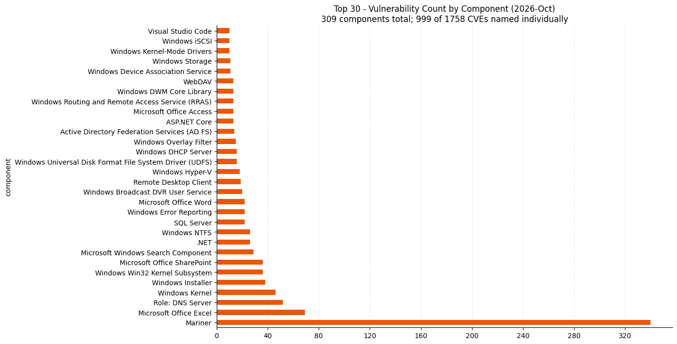
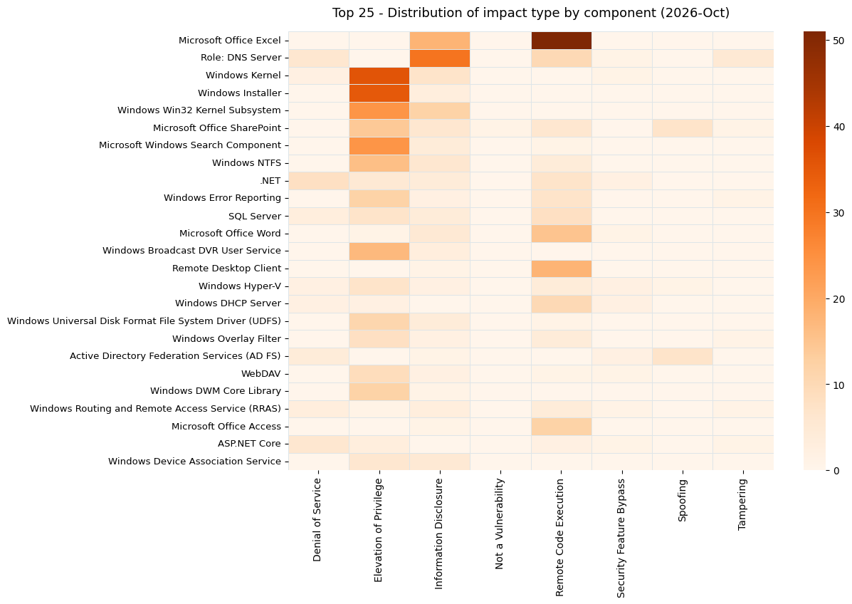
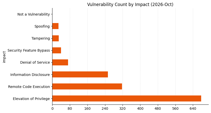
Microsoft is publishing 1,413 own-product vulnerabilities on October 2026 Patch Tuesday, including 1,102 vulnerabilities in Windows. Anyone who enjoyed last month’s record-setting Patch Tuesday will love the October 2026 edition, because it’s much bigger still. As Rapid7 has noted over the course of 2026, there is every reason to suppose that vulnerability volumes will continue to rise. Microsoft is aware of exploitation in the wild for just one of the vulnerabilities published today, as well as public disclosure for two others.
Windows Shell: zero-day security feature bypass
The Windows Shell is Microsoft’s term for the GUI interaction logic for the entire OS provided by explorer.exe and associated libraries and APIs, and for the second time this year, the Windows Shell is the site of an exploited-in-the-wild zero-day vulnerability. Today’s specimen is CVE-2026-96951. Once again, the immediate prize for an attacker is a Mark of the Web (MOTW) bypass. What this means is that Windows won’t provide the user with a dialog explaining that Windows protected their PC, because in this case, it didn’t. Exploitation requires that a user opens a specially crafted malicious file or visits an attacker-controlled site, so the evergreen advice about being careful what you click remains valid. Fans of vintage operating systems should note that Windows Server 2012 doesn’t receive a patch, although Server 2012 R2 does. The advisory acknowledges reporters from multiple organizations, although none from within Microsoft. The vulnerability also affected Microsoft’s Outlook.com cloud services, although Outlook.com was patched in a build dated several weeks ago.
.NET Framework: zero-day security feature bypass
Microsoft is aware of some level of public disclosure of CVE-2026-108398, a .NET Framework security feature bypass. Exploitation requires an attacker with an existing foothold to register a malicious .NET assembly for loading by a protected process, bypassing Windows Defender Application Control (WDAC) enforcement. Microsoft rebranded WDAC as App Control for Business several years ago, so you may know it under its new name. The Microsoft Learn page for Application Control for Windows points out that “your organization’s data is one of its most valuable assets… and threat actors want it”, and this is, of course, correct. The patch presumably removes an attacker-controlled location from the list of places .NET Framework searches for registered assemblies, which are typically contained within DLLs and executables. If any further indications were needed that vulnerability volumes are increasing industry-wide, this is only the second month that Microsoft has published vulnerabilities with six-digit CVE numbers, but these extra-large CVEs will seem unremarkable from now on.
Outlook: multiple no-interaction RCEs
The sheer volume of vulnerabilities in recent Patch Tuesday releases can easily include several examples of potentially concerning vulnerabilities, each of which might have been more remarkable in its own right back when volumes were lower. Today, Microsoft has published five separate remote code execution vulnerabilities in Outlook where the preview pane is a vector, meaning that simply scrolling past an email in the Outlook reading pane would be sufficient to trigger exploitation. Worse still, Outlook might helpfully display the preview without any user interaction at all. All five of CVE-2026-70242, CVE-2026-97749, CVE-2026-97016, CVE-2026-88156, and CVE-2026-70291 receive fixes in the same patches. No-interaction Outlook preview pane vulnerabilities can sometimes feature prominently in state-backed actor campaigns, with CVE-2023-23397 as a prominent example in this category.
Edge: security updates unclear
In September 2026, Microsoft did not appear to publish any desktop browser security advisories between the start of the month and Patch Tuesday. In October, a slightly different approach has emerged: several recent entries in the Edge security updates release notes mention new versions of Edge which incorporate the latest updates from the Chromium project, but without detailing which vulnerabilities have been fixed, stating instead, “CVE’s will be added as soon as available,” and directing readers to the Security Update Guide (SUG). At the time of writing, the SUG lists a total of zero vulnerabilities addressed in Edge in the first 13 days of October, and the “CVE’s added soon” message has been up for over a week. As a result, defenders have no obvious way of knowing which recent vulnerabilities Microsoft has addressed in Edge.
Microsoft lifecycle update
In Microsoft product lifecycle news, today sees Windows 11 24H2 Home & Pro reach end of servicing, while Windows Server 2022 moves to extended support, with free critical security updates continuing but no further feature development. Also this month, the final curtain falls for Windows Server 2012 and 2012 R2 with the expiry of the third and final year of cash-for-updates Extended Security Update (ESU) program for these aging workhorses. Microsoft lists the end of ESU Year 3 on October 14, 2026, in both cases. Microsoft has a long history of providing at least some security patches for products beyond the end of support, with Server 2008 being a case in point, but the time to move past Server 2012 is now. Office 2021 also moves into retirement on October 14; this includes the Long-Term Servicing Channel, with no ESU available in that case.
Also on October 15, 2026, Exchange Server 2016 and Exchange Server 2019 finally join the “no ESU” club, after two previous six-month reprieves. Microsoft seems to really mean it this time, since any future Exchange Server CVEs released by MSRC will stop mentioning Exchange 2016 and 2019. However, Microsoft points out that a lack of warnings does not mean those unsupported versions are not vulnerable to future security issues.
Summary charts
Scope workloads and share resilience policies with AWS Resilience Hub
Post Syndicated from Sinisa Mikasinovic original https://aws.amazon.com/blogs/architecture/scope-workloads-and-share-resilience-policies-with-aws-resilience-hub/
A resilience plan is useful only while it reflects the application you run. After a migration or deployment, a service can acquire a new dependency while its documented recovery objectives stay the same. In a shared Kubernetes cluster, even deciding which resources belong to that service can take investigation.
On September 18, 2026, the Next generation of AWS Resilience Hub introduced three capabilities to help you keep workload scope and resilience requirements aligned with your running environment:
- Amazon Elastic Kubernetes Service (Amazon EKS) label support for service input sources selects Kubernetes resources using the labels that already describe your workloads.
- Generative AI-powered Dependency Insights analyzes a service’s discovered dependencies and highlights the patterns worth reviewing.
- Resilience policy sharing through AWS Organizations lets a central team define resilience requirements once and make them available to member accounts.
In this post, you follow a team reviewing the resilience of a sample workload named checkout on Amazon EKS, representing an online store’s checkout service. The team starts by defining which Kubernetes resources belong to checkout, using labels to distinguish it from inventory in the same namespace. This establishes the resource boundary for the resilience review.
With that boundary defined, the team examines discovered dependencies and uses Dependency Insights to prioritize findings for investigation. A cross-Region dependency becomes a concrete question about whether checkout’s recovery design accounts for the services it requires to operate. The service owner then works with a central resilience team to validate the recovery requirements and apply a shared policy. Maintaining those requirements centrally gives teams a common definition to adopt across accounts, while policy events help the central team track adoption.
You perform these steps using the console or the AWS Command Line Interface (AWS CLI). The workload generates synthetic traffic to demonstrate dependency discovery.
About the application model: In the Next generation of Resilience Hub, the primary unit of assessment is a service. Services can be grouped into systems, and user journeys describe paths through them. See the key changes and the overview of the new hierarchy in the Next generation of Resilience Hub.
Prerequisites
To follow the examples, you need:
- Access to the Next generation of AWS Resilience Hub in a supported AWS Region.
- An Amazon EKS cluster with sample, labeled workloads and permission to configure access to the cluster.
- If you follow the CLI examples, install or update the AWS CLI using the installation and update instructions. Your installation must support the resiliencehubv2 commands. These examples use Bash.
- An AWS Identity and Access Management (IAM) role that Resilience Hub can assume, with the
AWSResilienceHubV2AssessmentExecutionPolicymanaged policy attached. The console can create this role when you create a service. - Kubernetes RBAC permissions and an EKS access entry that grant this role access to Kubernetes resources. The permissions guide provides the manifest and commands.
- For policy sharing, an organization with all features enabled and access to its management account.
The examples use two accounts: a workload account containing the EKS cluster and Resilience Hub service, and a management account that owns the shared policy.
For the CLI examples, configure profiles named workload and management for the respective accounts. Replace the example cluster ARN and other placeholders with your own values, and set the Region:
Each command uses --profile to select the account. Follow either the console steps or their CLI equivalents for each operation.
Amazon EKS label support for service input sources
A service input source tells Resilience Hub where to discover a service’s resources. Input sources can be AWS CloudFormation stacks, Terraform state files, resource tags, or Amazon EKS clusters. For an EKS input source, you select the namespaces to include. With this launch, you can also use Kubernetes label selectors to filter resources within those namespaces.
A namespace can contain workloads owned by different teams. With labels, you can select checkout’s resources without including inventory or reorganizing the namespace for an assessment. You use the same labels your teams already maintain.
How it works
Specify the cluster and one or more namespaces, then add label selectors to filter resources within each namespace. A selector contains a key, an operator, and values. Selectors within a namespace use AND logic: an object must match all of them. Without a selector, Resilience Hub discovers every supported object in the selected namespaces.
Checkout and inventory share the production namespace. Their resources carry app=checkout and app=inventory, respectively. Selecting production with app In checkout includes checkout’s Deployment and ReplicaSet and excludes inventory.
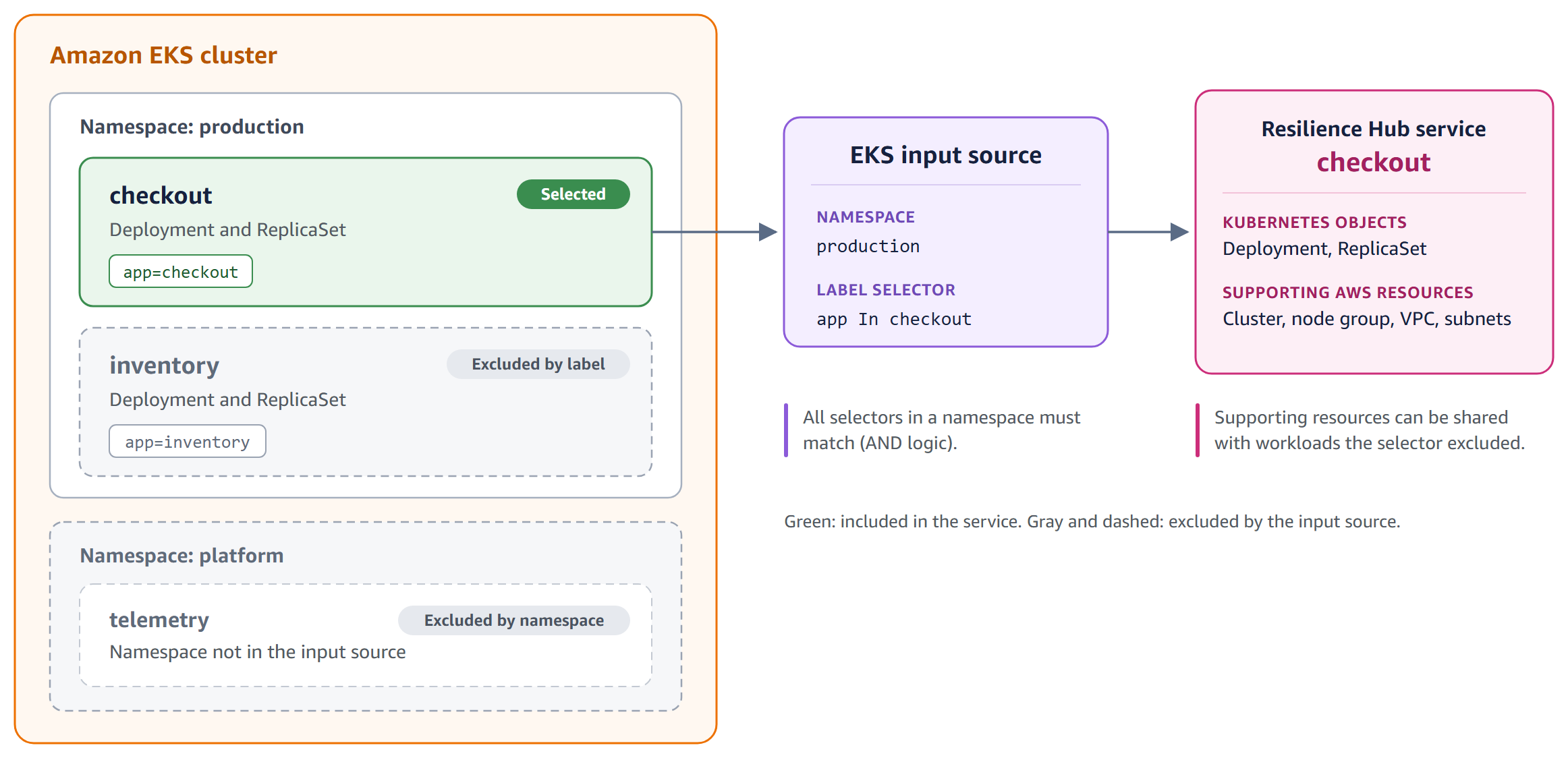
Figure 1: Selecting checkout resources with a Kubernetes label
The resource list also includes supporting AWS infrastructure, such as the cluster, node group, virtual private cloud (VPC), and subnets. Labels select Kubernetes objects. They don’t make that shared infrastructure exclusive to checkout.
How to use it
In the Resilience Hub console:
- Choose Create service and enter a name. Under Permission, choose Create default role to create an IAM role with the required AWS permissions, or choose Use another role to select an existing role.
- Under Service resource discovery, choose Amazon EKS cluster and enter the cluster ARN.
- Choose Configure namespaces, enter
production, and add a label selector with keyapp, operatorIn, and valuecheckout. - Choose Save, select Enable dependency discovery for this service, then choose Create service. Resource discovery starts automatically.
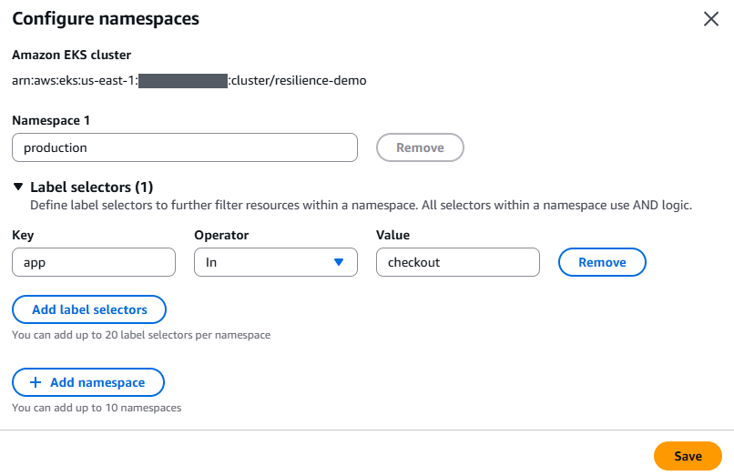
Figure 2: Scoping the checkout service to one namespace and one label
If you prefer to use the AWS CLI instead of the console, run the following commands to create the service and add its EKS input source.
Skip this block if you already created the service using the preceding console steps.
The console displays selector operators as In, NotIn, Exists, and NotExists. In the API, use IN, NOT_IN, EXISTS, and DOES_NOT_EXIST, respectively.
In the following command, replace ResilienceHubRole with your service’s IAM role name.
After resource discovery completes, you can use the following command to list the discovered resource types. If you created the service on the console, first set SERVICE_ARN to that service’s ARN.
Generative AI-powered Dependency Insights
Dependency Insights uses generative AI to summarize discovered dependencies and highlight patterns that warrant resilience review. It provides an overview and categorized findings.
The Resources list describes the service’s components. The Dependencies list shows endpoints discovered through DNS activity, including AWS service endpoints in other Regions and external APIs. When that list grows to hundreds of entries, Dependency Insights helps you prioritize what to investigate.
How it works
Dependency Insights builds on dependency discovery, an optional, separately priced feature. Dependency discovery analyzes DNS activity through Amazon Route 53 Resolver and does not require installing an agent in your workload. It examines up to 35 days of available history and continues monitoring for changes. The dependency list shows each endpoint’s name, location, and when it was first and last seen.
Dependency Insights analyzes this list, filters out common service activity that typically does not indicate resilience risk, and highlights patterns such as these:
| Pattern | What to investigate |
| Cross-Region dependencies | Whether a call to another Region is intentional, and how it affects recovery |
| New dependencies | Whether an endpoint first observed within the last seven days changes the documented architecture |
| Third-party dependencies | How the service behaves when an external provider is unavailable |
| Uneven usage | Whether activity reflects a scheduled job or a dependency used only at certain times |
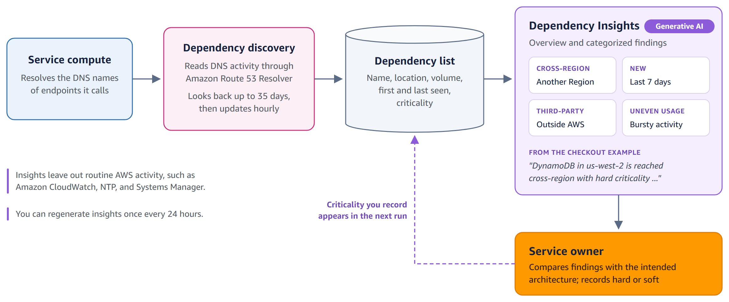
Figure 3: Turning dependency data into a focused review
Insights prioritize review. They don’t prescribe fixes or list every dependency. Use the full dependency list when you need detail. A new workload’s insights reflect only the history it has generated.
How to use it
In the Resilience Hub console, wait for initial dependency discovery to complete before generating insights:
- Open the service. On the Assessment tab, scroll to the Dependencies section to review discovered dependencies.
- Choose Generate insights.
- Read the overview and compare each finding with the intended architecture.
You can regenerate insights once every 24 hours. This limit applies whether you generate them through the console or the AWS CLI.
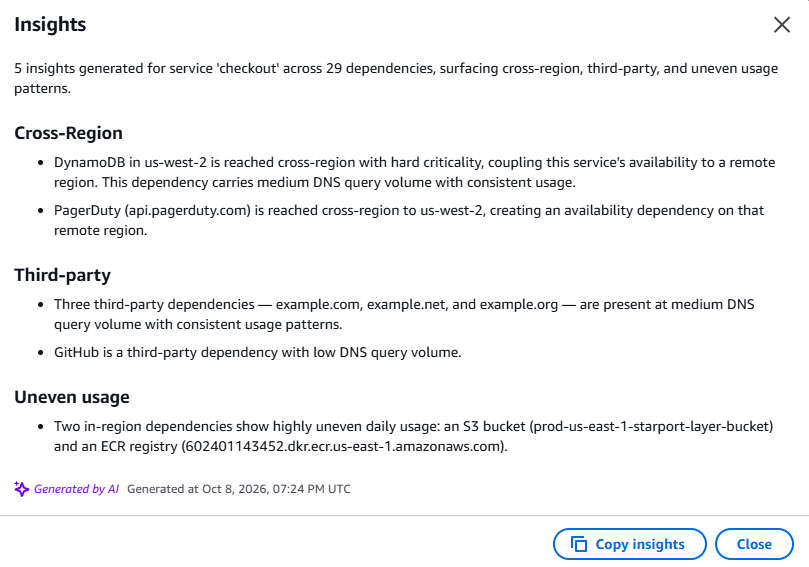
Figure 4: Dependency Insights for the checkout service
If you prefer the AWS CLI, use the following commands instead of the console steps. Set SERVICE_ARN to your service’s ARN.
Enable dependency discovery only if it is not already enabled. After initial discovery completes, review the dependency list and generate insights. If you already generated insights on the console, skip start-dependency-insights and use get-dependency-insights to retrieve the existing result.
Generation can complete asynchronously. Run get-dependency-insights again if the returned status is IN_PROGRESS.
The checkout service produced five insights across 29 dependencies. The following response shows the generated overview and all five findings:
The first finding identifies a cross-Region Amazon DynamoDB dependency. If checkout requires that dependency to accept orders, a disruption in the remote Region could prevent it from operating even when its Amazon EKS resources remain healthy. The service owner should verify which operations require the table and review how those operations behave when it is unavailable. That review determines whether the dependency fits the recovery design or whether the architecture needs to change. DNS activity alone cannot answer that question.
The uneven-usage finding points to container image infrastructure. Image downloads during pod startup can produce bursts of DNS activity. This is a pattern to investigate, rather than evidence that your application has an outage.
Classify a dependency as hard if the service fails without it, or soft if the service degrades but keeps running. In the sample environment, we had classified the DynamoDB dependency as hard using the following command. The comment describes an illustrative failure assumption, which requires validation through testing:
Resilience policy sharing through AWS Organizations
After reviewing checkout’s dependencies, the service owner can validate its recovery requirements with the business and the central site reliability engineering (SRE) team. Dependency findings inform that discussion. They don’t automatically determine the policy targets.
The central SRE team can codify the agreed requirements into a resilience policy, defining availability and recovery targets for critical services. The management account or a delegated administrator can share that policy across the organization so service owners can apply the centrally maintained requirements without creating separate copies.
The policy owner can review attachment and detachment events to track adoption. If a service stops using the policy, the SRE team can engage its owner to understand why and determine whether different requirements are appropriate. Application owners remain responsible for meeting the targets.
How it works
A policy can combine four target types: availability, recovery from an Availability Zone disruption, recovery from a Regional disruption, and data recovery. The recovery time objective (RTO) specifies the targeted recovery time. The recovery point objective (RPO) specifies the tolerable period of data loss.
When sharing is on, the policy appears in every member account alongside the account’s own policies, and its ARN shows which account owns it. Each service owner chooses whether to apply it. If a requirement must apply regardless of that choice, associate the policy with a system containing the relevant services instead, as described in Applying resilience policies across accounts.
The owning account can review a timeline of the services that start or stop using the policy. Turning sharing off stops evaluating member services against the policy and removes it from the services that used it, so coordinate changes with the teams involved.
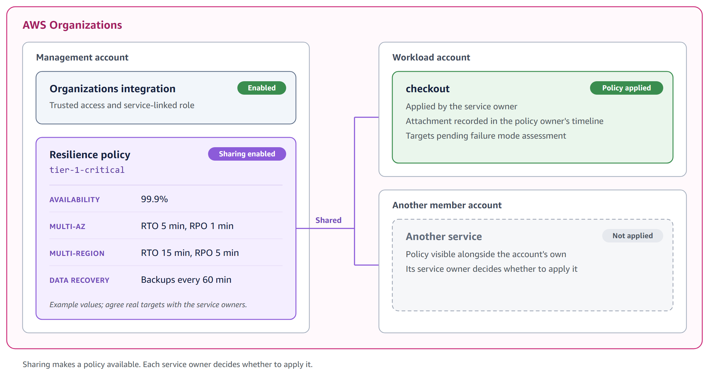
Figure 5: One policy definition, shared with member accounts
How to use it
The organization integration is a one-time setup in the management account:
- In the Resilience Hub console, open AWS Organizations settings.
- Select Enable trusted access and create a service-linked role, then choose Create integration.
To confirm that the service-linked role exists in a member account:
Next, create the policy in the management account with sharing turned on. Policy names can contain letters, numbers, hyphens, and underscores, but no spaces. The following targets are examples. Agree on real values with the business and service owners. This example uses an availability target of 99.9 percent.
In the workload account, find the shared policy and apply it to the service. On the console, choose Change policy on the service and select the shared policy. With the AWS CLI:
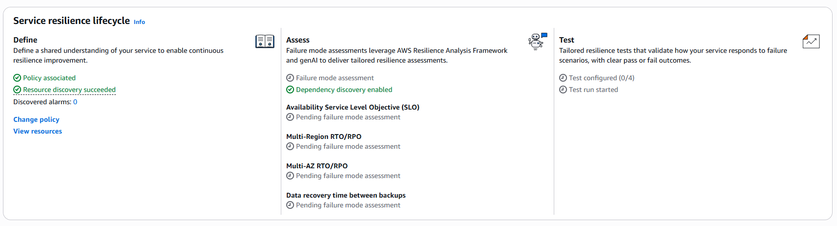
Figure 6: Policy targets are defined. Assessment of those targets is still pending
Back in the management account, the policy owner can confirm adoption:
An attachment event confirms adoption, not compliance. After we applied the shared policy, the console changed each target from Not defined in policy to Pending failure mode assessment. A failure mode assessment and appropriate resilience testing are needed to determine whether the service meets those targets.
Things to know
- Shared clusters. Labels decide which Kubernetes objects belong to a service. On a cluster that several workloads share, review the discovered dependencies to confirm they belong to the service, as described in the guidance for shared EKS clusters.
- What DNS-based discovery can’t see. Connections made directly by IP address aren’t discovered, AWS Lambda functions need VPC connectivity to be covered, and very infrequent calls might not appear in initial results. See Coverage and known limitations.
- Timing. Results reflect the history available to the service. Give a new workload time to build history before drawing conclusions from its insights. You can regenerate insights once every 24 hours.
Cleanup
If you created resources to try these capabilities, remove them when you finish. Turning sharing off also removes the policy from every member service that uses it, so only do this for a demonstration policy:
Delete the EKS cluster as well if you created it only for this walkthrough.
Conclusion
Start with a service whose architecture and ownership you know. Use EKS labels to check its Kubernetes resource boundary, then review Dependency Insights against its intended behavior. If several teams maintain the same requirements separately, consider a shared policy.
You can use the capabilities together or independently. Label support applies to EKS workloads. Dependency Insights and policy sharing also support services beyond EKS. Insights focus the investigation. Your architecture review determines what to change.
Further reading
- What changes with Next generation Resilience Hub
- Viewing discovered dependencies
- Dependency Insights considerations
- Sharing a policy across your organization
- Setting up Organizations integration
About the author
Should Elon Musk and Jeff Bezos Work Together to Get to the Moon?
Post Syndicated from The Atlantic original https://www.youtube.com/shorts/e3gljKiS2xA
Part 2 – Cybersecurity journeys: What even is this job?
Post Syndicated from Shannon Brazil original https://aws.amazon.com/blogs/security/part-2-cybersecurity-journeys-what-even-is-this-job/
If you’ve ever looked at a list of cybersecurity jobs and felt like none of them fit you, you might just be looking at a short list. Most career guides cover the same few roles, like the analyst watching alerts or the pen tester (penetration tester, someone hired to legally break into systems to find weaknesses) looking for a way in. Those jobs matter, but they’re a small slice of a field with room for a lot of different skills. The three people in this post do work you probably won’t find in those guides, and none of them started out qualified for it. What they had in common was a willingness to aim at something before they were ready and to build the skills on the way there. If you’ve ever talked yourself out of a role because you didn’t tick every box, their stories are worth a few minutes, because the move each of them made is one you can make too.
In Part 1: I didn’t plan this, I shared how three people found their way into security from a warehouse floor, a marketing desk, and a teenager’s bedroom. This week is about where people end up after they’re inside. I’ve been in security for over a decade, and while putting this series together I kept running into work I hadn’t come across before: measuring the risk of a million applications at once, building detection tools from the customer service side of the house, and thinking seriously about how to secure infrastructure that’s being launched into orbit.
The skill tree

Jason Lane, Security Engineer
When Jason Lane told me he plans his career like a Dungeons & Dragons character build, I assumed he was being metaphorical, but he meant it literally. “Think of it like a video game skill tree,” he said, and then walked me through the whole framework. You start by picturing your level 20 character, the version of yourself with the skills and the role you actually want, and then you work backward. At level 19, what choices get you to 20? At level 18, what needs to be true so you even have those options? You keep stepping back until you’re standing at level 1, looking at a path you built from the top down.
For Jason, level 20 was vulnerability research (finding unknown security flaws in software before attackers do). At the time he was a systems administrator, keeping servers and networks running, which gave him a solid grasp of how systems fit together but little exposure to picking apart the applications on top of them. That gap, application security, was the next node on his tree, so he called an IT recruiter, laid out his plan, and was honest about where he stood. The recruiter found a credit card processing company that needed an application security engineer and was open to someone who wasn’t one yet. For Jason it was a paid apprenticeship in the exact skill he was after; for the company it was a motivated engineer who would grow into the role. He describes it as a deal where both sides got what they needed, and that framing matters: he wasn’t settling for less, he was trading a steeper learning curve for a faster path to where he wanted to be.
He spent 4 years there taking applications apart to understand what made them breakable, and when he had learned what that role could teach him, he applied the same framework again. A friend offered to get him an interview at Google, and Jason’s honest reaction, that he wasn’t smart enough to work there, is the kind of self-doubt most of us recognize (also known as imposter syndrome). His friend didn’t buy it, the interviewers didn’t either, and they hired him. The lesson he took from it is one worth borrowing: the voice telling you that you don’t belong in the room is often wrong, and the way to quiet it is to put in the work until the skills speak for themselves. He went on to spend nearly 7 years doing Android vulnerability research, the kind of deep technical work most companies don’t have the budget for.
That track record opened the door to Amazon. When the team that measures application risk interviewed him, the hiring manager’s pitch was simple: we could really use your vulnerability research experience. Years of tearing systems apart to find what made them breakable turned out to be the perfect background for judging which systems were most at risk. Today, Jason measures risk across roughly a million applications at Amazon, evaluating which ones would cause the most damage if compromised and which are most likely to be targeted, so the organization can focus on the most dangerous ones first. When his manager recently presented the team’s work to a new senior leader, the example he used was a project Jason had built from scratch. Jason’s name wasn’t on the slide, and he told me he didn’t need it to be, but you could hear the pride in his voice.
When I asked what he’d tell someone with a big vision and no idea where to start, he said to get obsessively clear about where you’re going, because the gaps will show up on their own. He compared it to planning a 100-mile trip and realizing you aren’t wearing shoes; once you see it, you can’t unsee it. And if it turns out the dream is really a hobby, he’s at peace with that too.
| “If you can wait for Saturday, maybe you should just wait for Saturday. There’s nothing wrong with that.” —Jason Lane |
If you’ve been waiting for someone to hand you a career ladder, Jason’s approach offers another option: decide where you want to end up, and let that tell you what to learn next.
Full circle

Jason Goodman, Security Engineer
Where Jason Lane planned his career from the finish line, Jason Goodman’s career has looked more like a pinball machine, bouncing through three security disciplines in about a year and picking up new skills along the way.
The foundation was laid long before he knew it. Eight years ago, before Amazon acquired Ring, he was working in customer service, troubleshooting doorbells and helping customers with their accounts, and before that he sold computers at Best Buy. “That was the most tech I had,” he told me, grinning. What pointed him toward security was partly a nudge from his father-in-law, who worked in IT, and partly what he was seeing on the phones every day: the occasional account access that didn’t look right, the quiet signals that something might be off. Those patterns made him want to understand the systems behind them, so while he was still in customer service he went back to school for a cybersecurity degree.
He didn’t wait until graduation to start building toward the move. He reached out to the manager of the internal threat team (the people who look for misuse of access from inside an organization) and asked a question anyone can ask: what could I do to keep progressing while I’m in school? That turned into stretch projects, and here is the part worth noticing, he earned the bigger ones by delivering the smaller ones first. His standout project was a fraud prevention dashboard that helped the team spot potential misuse of customer account access, a blind spot nobody had flagged. He had the credibility to be handed it because he’d already shown up for the low-stakes work, and it opened the door to his first security engineering role on that same team.
From there he moved to an adversarial threat detection team (the people who watch for outside attackers trying to get in), which meant flipping his mindset overnight: instead of asking what someone on the inside could do with their existing access, he was now asking how someone on the outside would try to break in. A later move took him into application security, where the work shifted from responding after the fact to building security into processes from the ground up.
| “I’m in my third discipline in a year since transitioning out of customer service into security engineering.” —Jason Goodman |
What I find fascinating is how much carried over from one role to the next. The Splunk queries (Splunk is a tool for searching and analyzing large volumes of log data) he learned in customer service carried into internal threat work, the detection logic from insider investigations carried into adversarial detection, and now in application security he has come full circle, working alongside the same customer service teams he started with, except this time he’s helping build the security around them.
Through all of it, he has leaned on four different mentors, and the way he found them is worth stealing. Finding one mentor who truly invests in you is hard; finding four is rare. Jason didn’t wait to be assigned anyone. He reached out to people whose work he admired, starting with that internal threat manager during school, asked specific questions, and stayed in touch over the years as he grew. Each mentor served a different purpose: one for navigating school, one for stretch projects, one for learning to think like an adversary, and one for getting grounded in application security. “I’ve always felt like I could take at least a little nugget from each one of them,” he said. Next on his list is offensive security, meaning pen testing and red teaming (simulating real attackers to test how well an organization defends itself). He figures starting on defense was the right call: learn what attackers do and how to stop them, then learn to think like one.
If your current role feels unrelated to security, Jason’s story is a good reminder that the skills you’re building now may be exactly the ones your first security job needs. The analytical habit of noticing when something is off, the patience to explain a problem clearly, even the instincts you pick up from a completely different field all transfer. The trick is learning to name what you already have and point it at the work you want.
The edge of the map

Harshvardhan Chunawala, Solutions Architect, AWS Startups
Harshvardhan Chunawala was still in high school when he started finding security flaws in real products and reporting them to the companies that built them. He had started out building websites and web applications, and after he understood how software was put together, he couldn’t stop wondering how it could be pulled apart. Rather than wait until he had a degree or a job to explore that, he began poking at real products on his own, and when he found a flaw he contacted the company and worked with them to fix it.
Today he advises startup founders at AWS on security and volunteers his time to teach cloud and security courses to students, who often ask him where to start when entry-level work is being automated. His answer has changed over the years. Now that generative AI can answer the surface-level questions, he believes curiosity matters more than credentials, because the people who stand out are the ones who keep asking questions after the tool runs out of answers.
| “AI tools put everyone on the same starting line. Interest and passion has become the driving force.” —Harshvardhan Chunawala |
What surprised me most, though, was where his own curiosity took him. While studying at Carnegie Mellon University (CMU), he ended up working on space missions, including time as a mission operator for the Iris lunar rover (Iris and CMU’s next rover, MoonRanger, appear with him in the photo above). If you had asked me a few years ago whether security belonged anywhere near a rover on the Moon, I wouldn’t have known what to say, but Harshvardhan would have answered right away: anything that can be commanded remotely can be commanded by the wrong person.
When I asked about the future of security, he took the conversation completely off the map. He talked about robots entering people’s homes and about data centers moving from land to underwater to space. A satellite has to be protected in orbit, where nobody can physically reach a compromised system, and on the ground, where the stations that command it are targets too. “So are cyber security specialists going to go under astronaut training?” he asked, grinning, and he was only half joking. He has already written a two-part guide to incident response for satellite operations on AWS, so for him, this corner of the map is already part of the job.
If you’re drawn to an area that doesn’t look like a security job yet, Harshvardhan’s story is worth taking seriously: the move he keeps making is to follow a question past the point where the easy answers run out, into territory nobody has fully mapped. You don’t need a satellite to do that. Pick the corner of technology that genuinely fascinates you, start asking how it could be attacked and defended, and you might find you’re standing at the edge of a role that doesn’t have a name yet.
The thread
These three stories share one thread: the job you end up loving might be one you haven’t heard of yet. Jason Lane mapped his moves in advance, Jason Goodman carried his skills through three disciplines in a single year, and Harshvardhan is already helping AWS customers secure satellites and the ground systems that run them. None of them could answer “what do you do?” in a single sentence, and I suspect that’s true for a lot of people doing interesting work in this field.
If you’re curious about the roles that exist beyond the ones you already know, here are a few places to start exploring:
- The NICE Workforce Framework for Cybersecurity lays out dozens of security work roles and the skills each one needs
- CyberSeek offers an interactive career pathway map showing how entry-level roles connect to advanced ones
- AWS Skill Builder has free security and cloud training you can start today
- CISA’s Cybersecurity Awareness Month page has more resources for this October
In Part 3: The work behind the work, we pull back the curtain on what the day-to-day of security actually looks like compared to what people imagine.
Have you found a corner of security most people don’t know exists? Share your story on LinkedIn!
Resolving concurrent write conflicts for Apache Iceberg tables in Amazon Redshift
Post Syndicated from Sanjay Devireddy original https://aws.amazon.com/blogs/big-data/resolving-concurrent-write-conflicts-for-apache-iceberg-tables-in-amazon-redshift/
In Getting started with Apache Iceberg write support in Amazon Redshift – Part 1, you learned how to create Apache Iceberg tables and write to them with INSERT. In Part 2, you modified data at the row level with DELETE, UPDATE, and MERGE. Both posts assumed your write had the table to itself. In production, that is rarely true: streaming jobs, scheduled pipelines, and one-time transformations frequently write to the same table at the same time. Amazon Redshift now resolves many of these concurrent writes automatically, committing changes that previously failed and were forced to retry. In this post, we explain why concurrent writes to Iceberg tables conflict, how Amazon Redshift resolves the conflicts that don’t actually overlap, how the engine escalates its checks from operations to partitions to individual files, and the throughput improvement it provides.
The challenge of concurrent writes
Apache Iceberg uses optimistic concurrency control (OCC) to keep a table consistent when more than one writer commits at the same time. Each writer prepares its changes against the table’s current version and commits by atomically advancing the table version in the catalog, on the condition that no other writer advanced it first. If another writer commits in the meantime, the condition fails and the entire write is discarded. This strictness maintains snapshot isolation semantics: if the later commit were applied anyway, it would replace the table version without the earlier writer’s changes, silently losing a committed write.
Readers don’t encounter this problem. An Iceberg scan always reads a committed snapshot, so a read is never invalidated by a concurrent write. That leaves write-write conflicts as the only case the engine must resolve, and resolving them correctly is what preserves snapshot isolation semantics for the table.
The problem is the bluntness of this check. The condition is evaluated against the table version, not against the rows or partitions each writer touched. At that grain, its answer is correct in that the version really did change. However, it says nothing about whether the two writes overlapped in the data underneath. Two writers that modified entirely separate partitions, or that independently inserted new data, conflict exactly as hard as two that rewrote the same rows. This happens whenever their query-start-to-commit windows overlap.
Consider a retail analytics platform with a customer_orders Iceberg table. A streaming pipeline might land new orders continuously with hundreds of inserts a minute. A nightly compliance job deletes records older than seven years, and takes about an hour to run. The two writes never touch the same data: the stream only adds recent orders, and the compliance job only removes old ones. Under basic optimistic concurrency, that doesn’t matter. If a single streaming insert commits at any point during that hour, the compliance job loses the race, its hour of work is discarded, and the next attempt re-scans terabytes of data only to re-enter the same race. The table version conflict was real even though the data conflict was not.
The common ways to avoid this are all manual, and each carries a cost. You can serialize your writers so that only one commits at a time, which gives up concurrency entirely. You can split a single logical table into several physical tables so that no two writers ever share one. This trades a clean data model and the ability to query across them for the ability to write in parallel. Or you can wrap every write in an application-side retry loop and absorb the cost of re-running statements that never actually conflicted. In each case, the effort goes toward working around the commit protocol rather than toward your data.
How Amazon Redshift resolves write conflicts
When a commit loses the race, Amazon Redshift now asks a more precise question before giving up: Did the writers that committed ahead of it actually change the same partitions or files or rows it changed? When the answer is no, there’s no reason to discard the work. Instead of aborting, Amazon Redshift rebases the change (similar to git rebase), replaying the already-prepared write onto the latest version of the table and committing that result. Both writes land, with no re-scan, no re-execution, and no retry loop in your application.
In the retail example, the compliance delete previously failed the moment a streaming insert committed inside its execution window. Now Amazon Redshift examines both writes, sees that the inserts only added data files while the delete only removed others, and confirms they never touched the same data. Because the changes are provably independent, Amazon Redshift rebases the delete onto the updated table version and commits it. Both writes succeed, the hour of work is preserved, and downstream consumers see both changes.
This behavior is automatic for eligible writes, with no clustering keys to choose, no repartitioning, and no setting to enable. When two writes genuinely conflict, the behavior is unchanged from today: the conflict surfaces and the later writer fails and must retry.
Two principles govern how the resolution works. The first is that a conflict is a matter of granularity. A failed race isn’t automatically a conflict. It’s a question that can be asked at different resolutions. The engine can ask whether any writer removed data at all or whether they only added it, and if data was removed, whether it came from the same partition, the same file, or the same rows that the current write touched. The finer the granularity examined, the more apparent conflicts turn out to be independent changes that can safely coexist. But finer checks also cost more: taken to the limit, the engine could intersect two change sets row by row, and that is expensive and usually unnecessary. So Amazon Redshift evaluates the least expensive level first and examines a finer level only when it must.
The second principle is that correctness takes precedence over concurrency. Conflict resolution works entirely from table metadata and never re-scans data or re-plans a query. When the engine can’t prove that two writes are independent, it doesn’t guess. It declines to resolve the conflict and the write retries, exactly as it would today. An unnecessary retry costs a small amount of time, whereas an incorrect resolution risks losing data, so the system is deliberately biased toward the safe outcome. Resolution operates under snapshot isolation, the same model Amazon Redshift already uses for Iceberg reads. Engines such as Apache Spark, Amazon EMR, and Amazon Athena honor it through the table’s isolation-level property, so a table shared across engines retains consistent semantics. For tables whose write isolation property is set to serializable, Amazon Redshift preserves the stricter contract and surfaces every conflict rather than resolving it. This is the Iceberg table property write.*.isolation-level. It’s unrelated to the Amazon Redshift database isolation level set with ALTER DATABASE … ISOLATION LEVEL, which governs Amazon Redshift transactions and has no effect on Iceberg commit conflict resolution.
Resolving at the right granularity
When a commit loses the race, the engine escalates through a sequence of checks, from the cheapest to the most precise. Each level is a complete resolution on its own and if a check proves the writes independent, the rebase commits and no finer check runs. The following diagram shows this escalation sequence: an operation-level check first, then partition-level, then file-level. Each level either proves the writes independent or escalates to the next, and a genuine conflict surfaces only after the last.
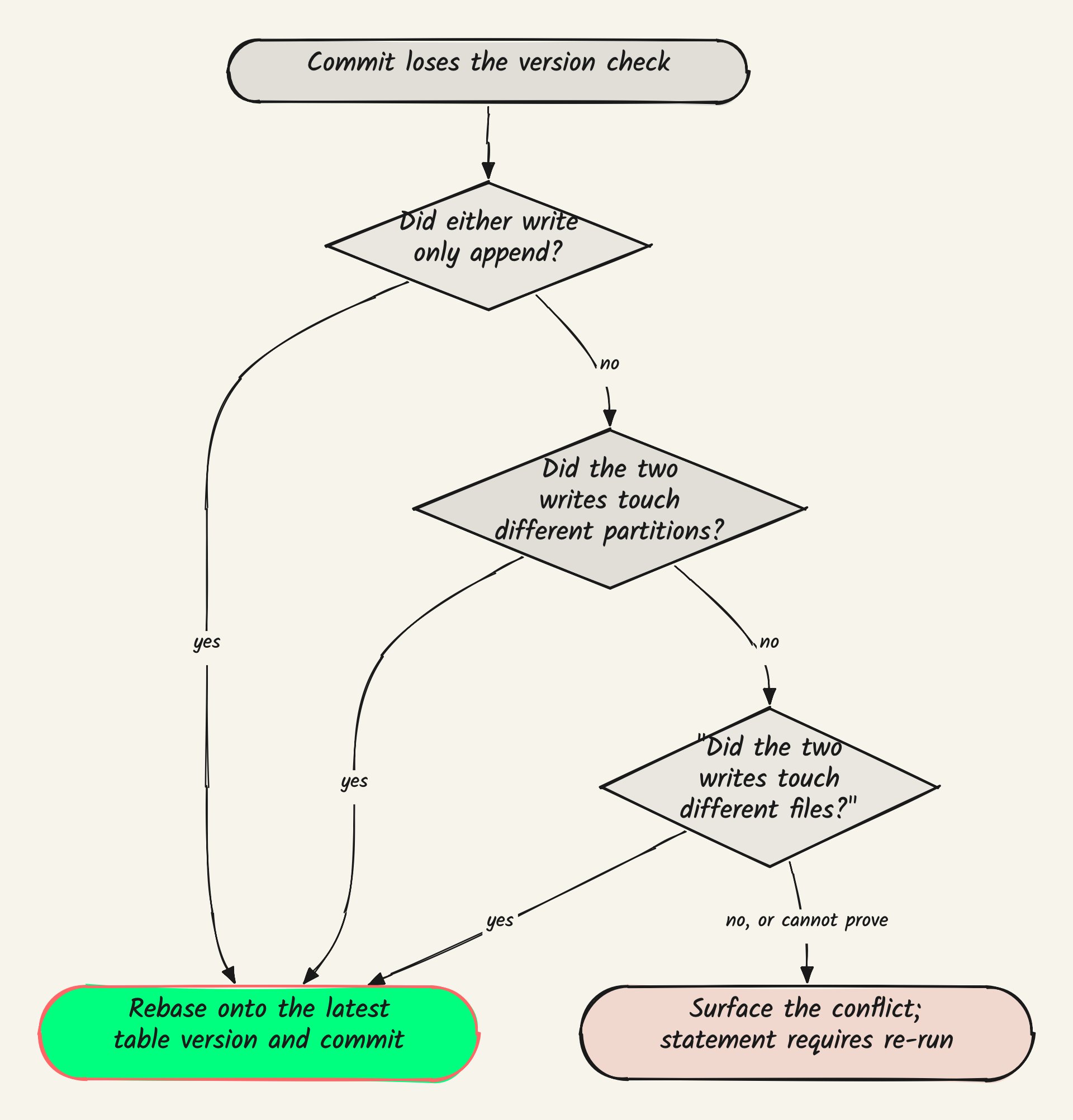
Figure 1: The conflict-resolution escalation from operation-level to partition-level to file-level checks
The first check is by operation. A write that only added data, for example an INSERT consisting of new data landing from a streaming job, can’t have removed anything another writer relied on, so any write can be rebased against it. This single rule resolves every combination in which at least one of the two writes only appended. A DELETE, UPDATE, or MERGE commits cleanly against a stream of concurrent inserts, and an INSERT commits cleanly over any other concurrent change, including a compaction.
Next, when both writes removed data, the engine compares the partitions they each touched. Writes that modified disjoint partitions, for example batch jobs updating different dates or per-Region pipelines maintaining their own slices of one table, are independent by construction and both can commit cleanly.
Finally, when both writes touch the same partition, the engine compares the individual files that each one changed. Two jobs deleting different rows of the same date partition usually land in different files, and when they do, both can commit cleanly. Only when two writes modified the same file does the conflict surface and the statement re-run. The protocol additionally has headroom for one further level: distinguishing changes to different rows within a single file.
The following table summarizes the outcomes by operation pair. Read down for the concurrent write that committed first, and across for your write.
| Your write ↓ / Concurrent write → | INSERT |
DELETE / UPDATE / MERGE |
Compaction | ALTER |
|
| 1 | INSERT |
Resolves | Resolves | Resolves | Re-run required |
| 2 | DELETE / UPDATE / MERGE |
Resolves | Resolves based on partitions or files touched. A same-file change surfaces as a conflict | Resolves based on partitions or files touched. A same-file change surfaces as a conflict | Re-run required |
| 3 | ALTER |
Re-run required | Re-run required | Re-run required | Re-run required |
Performance
To measure the effect, we ran an increasing number of concurrent writers committing to a single Iceberg table over a fixed window. We compared basic optimistic concurrency mode, where a losing commit is aborted and re-runs, against automatic conflict resolution mode being enabled. Every writer issued the same single-statement INSERT, so the only variable across the various runs was contention rather than workload. We scaled 1–16 concurrent writers and recorded, for each configuration, how many commits succeeded and how many were rejected as conflicts.
Setup: one unpartitioned Iceberg table registered in the AWS Glue Data Catalog in the US East (N. Virginia) AWS Region (us-east-1). Each writer is an independent session issuing autocommit INSERT statements in a loop over a 60-second period. We report the commits completed and the attempts rejected as conflicts for each configuration.
The first figure shows write throughput as writers are added, normalized to the single-writer case so the comparison doesn’t depend on instance type or table size.
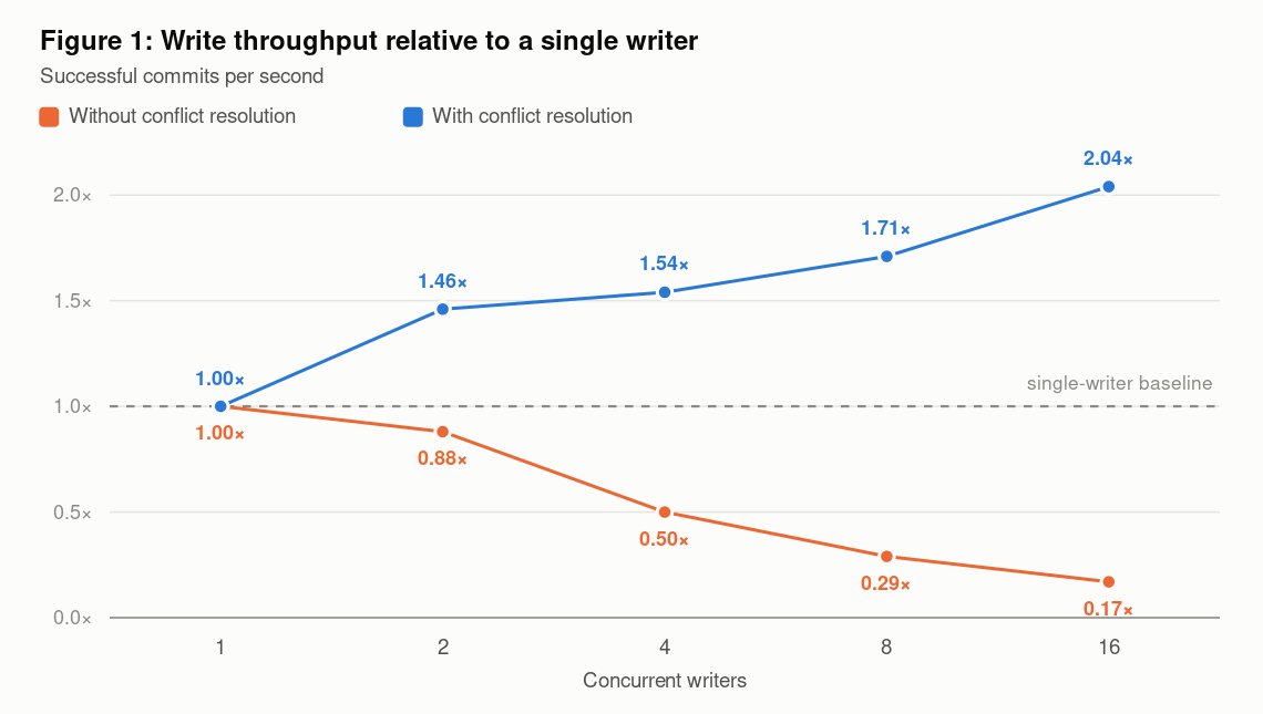
Figure 2: Write throughput as concurrent writers increase, with and without automatic conflict resolution
Under basic optimistic concurrency, adding writers makes writing to the table slower. At 16 writers, throughput falls to 0.17× of a single writer, because nearly every writer’s work is discarded and redone rather than committed. With automatic conflict resolution the same workload scales to roughly 2×, and no commit is rejected in any measured configuration. At 16 concurrent writers, 12× more commits complete in the same window. The second figure shows why.
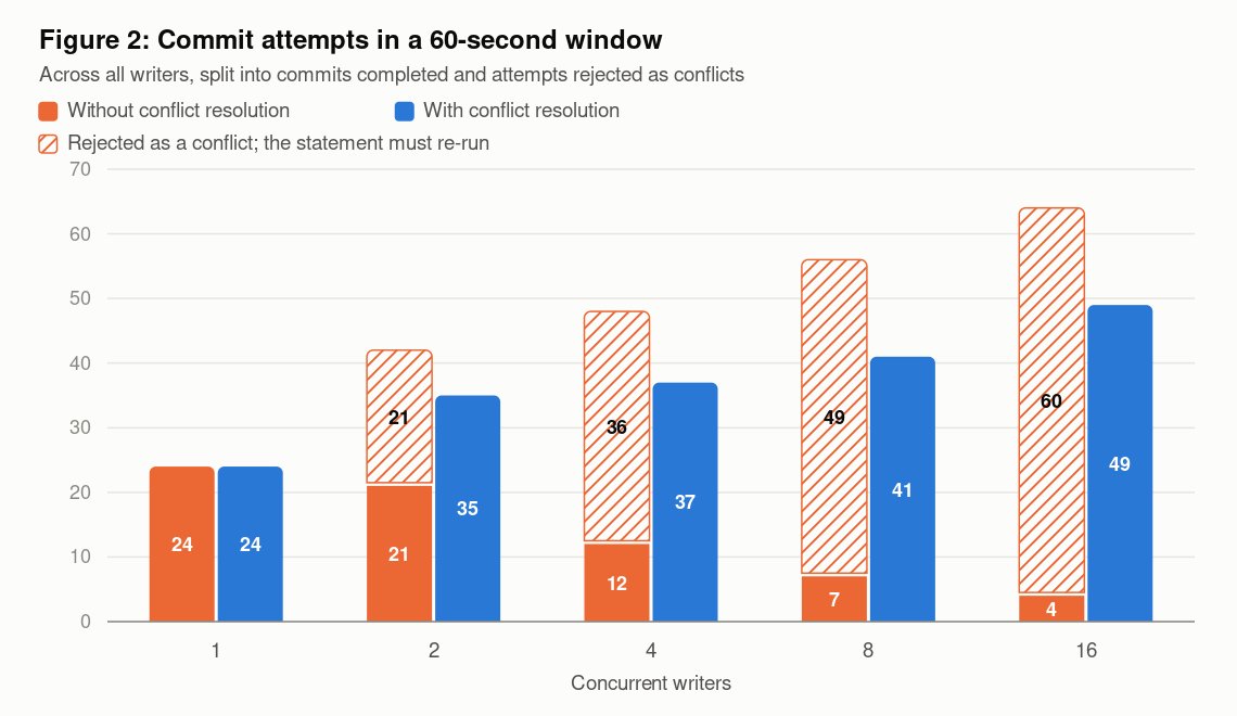
Figure 3: Commit failure rate as concurrent writers increase, with and without automatic conflict resolution
The baseline’s failure rate is almost exactly (N−1)/N, for example 50 percent at two writers, 75 percent at four writers, and 94 percent at 16 writers. This illustrates the table-level check that occurred previously: only one writer wins each commit round and every other writer in flight is rejected. Additional writers translate almost entirely into repeated work rather than progress. With conflict resolution enabled, the same runs record no conflicts at all, because every write in this workload is an append, and an append never removes data another writer relied on.
This benchmark isolates the most basic append case deliberately: a single unpartitioned table and insert-only writers, which is the pattern behind continuous ingestion. Workloads that remove data exercise the partition and file checks described earlier, where the outcome depends on whether the two writes touched the same partition and the same files.
Fleet Results
Before conflict resolution, concurrent-write conflicts were the single largest cause of failed Iceberg writes in Amazon Redshift, accounting for roughly one in five failed Iceberg write queries each week. We rolled out this feature in stages, beginning with the operation-level check that covers concurrent appends. As that stage reached full fleet deployment in early September 2026, conflict errors from concurrent writes dropped to nearly zero, even as Iceberg write volume on the fleet more than doubled. One residual spike shown below came from a workload issuing concurrent UPDATE statements, a conflict class that subsequent partition and file level checks will resolve as they deploy across the fleet.
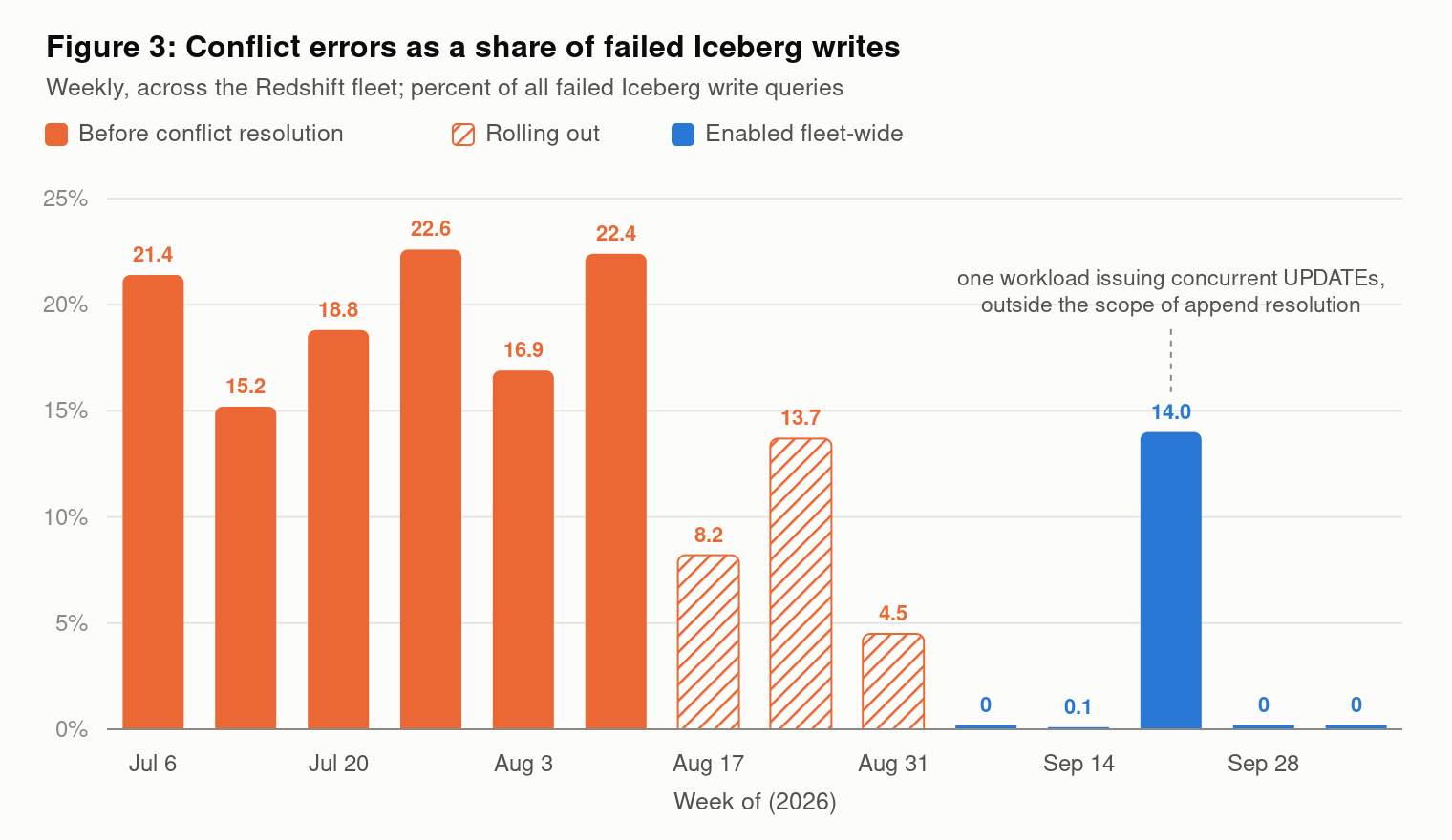
Figure 3: Conflict errors as a share of failed Iceberg writes
Observing conflict resolution
Every Iceberg commit attempt is recorded in the stl_iceberg_commit system table, including the outcome, the number of attempts, the concurrent operations the write rebased over, and the time spent rebasing. To see how often resolution is engaging on an example table:
Conclusion
Concurrent writes are a fact of production data lakes, and until now, they forced you to serialize writers, partition around the problem, or retry. With automatic conflict resolution, Amazon Redshift commits concurrent writes that don’t actually overlap. These include any mix of writes alongside concurrent appends, and row-level writes that changed different partitions or different files of the same table. To get started, write to your Iceberg tables from multiple jobs on patch 203 or later. Non-conflicting commits start to resolve on their own. To learn more about Iceberg write support in Amazon Redshift, see Part 1 and Part 2.
About the authors
Exploring AWS Lambda Web Functions for building web applications
Post Syndicated from Julian Wood original https://aws.amazon.com/blogs/compute/exploring-aws-lambda-web-functions-for-building-web-applications/
You can now run a standard Node.js web server on AWS Lambda with Lambda Web Functions, a new type of Lambda function. Deploy it with one command or AWS CloudFormation and get a public HTTPS endpoint with no adapter layer and no servers or load balancers to manage.
Lambda Web Functions suit server-side rendered web apps, REST and GraphQL APIs, streaming endpoints, and microservices. Building on the launch announcement, this post uses a sample application to show how one execution environment handles many requests at once and how the same app serves a global audience. See how active-CPU billing keeps the cost of waiting low while your code waits, with memory and requests billed separately.
Overview
Lambda launched in 2014 with a minimal model: upload your code, and the service handles everything else. For over a decade that code ran as an event handler, invoked once per event such as a batch of queue messages or an object landing in Amazon Simple Storage Service (Amazon S3). We now call this an Event Function and it remains the right choice for event-driven work.
Web Functions are a second type of Lambda function, running on the same Firecracker-based isolation as Event Functions. Instead of a handler that receives an event, your code runs as a standard HTTP server that listens on a port, which is what lets a web framework, or in this case a plain Node.js server, run unmodified.
A Web Function is made of three resources:
- Web Function is the top-level resource with a name and configuration.
- Revision is an immutable snapshot of your code and configuration which Lambda creates each time you deploy code or change revision configuration, so you can roll back by routing traffic to an earlier revision.
- Endpoint is a network entry point with a unique HTTPS domain, an authentication type, and the rules that route traffic to your revisions.
At launch, Web Functions run Node.js 24 on Arm64, with 2 vCPUs and 2 GB of memory per execution environment. Web Functions support Amazon Virtual Private Cloud (VPC) connectivity, allowing your function to access resources that exist within a VPC.
Walkthrough
Node.js frameworks that start an HTTP server, such as Express, Fastify, and Hono, run without adapters. Next.js in standalone mode needs a small index.js that sets its host and port. This post uses a plain Node.js server to stay dependency-free.
The full source is available in the Serverless Patterns collection along with other Web Functions patterns.
Prerequisites
You need an AWS account with the AWS Command Line Interface (AWS CLI) installed and configured and Node.js installed locally.
The pattern instructions show how to clone the repo and change to the pattern directory or download the pattern .zip file to run the example.
The app
The dashboard is a single Node.js HTTP server that streams live server metrics to the browser over server-sent events (SSE).
The runtime provides the address to listen on in the AWS_LAMBDA_HTTP_ENDPOINT environment variable, in host:port form. The server reads it and starts listening, exactly as it would anywhere else:
The runtime is nodejs24.x, and it loads index.js at the package root by default. To use a different entry file, set AWS_LAMBDA_NODEJS_ENTRYPOINT to its path.
Run locally
You can run the server locally with npm start.
Browse to http://localhost:3000/ to view the dashboard streaming from the local server.
Deploy
- Deploy using the single command:
For this example, you can also use
npm run deploydefined in thepackage.jsonfile.
The AWS CLI bundles your code, creates the function and an endpoint named dev with a live HTTPS URL. It also creates an execution role and a versioned S3 bucket, if one does not exist, that all CLI-deployed Web Functions in the Region share.
- Press Enter to create the resources.
The AWS CLI output shows the URL in the format: https://<id>.<shard>.lambda-web.<region>.on.aws
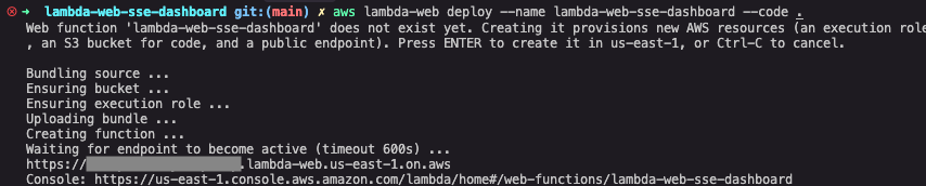
Figure 1: AWS CLI showing the aws lambda-web deploy command.
Browse to the URL and the dashboard loads, already streaming. This endpoint is public and the sample has no authentication, so use it for evaluation and delete it when you finish.
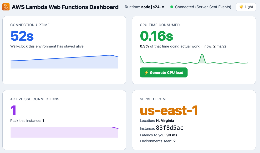
Figure 2: The app streaming dashboard showing function information.
The dashboard shows how long the execution environment has been alive and how many streaming connections it is holding open. It shows how much CPU it has used with a button to generate real CPU load on demand. The function runs in the US East (N. Virginia) Region (us-east-1). From my laptop in the United Kingdom, latency is 90 ms.
The dashboard updates every two seconds over a single HTTP streaming response. A Web Function environment is a long-lived process, so it keeps the connection open and keeps pushing data to the browser. The long-lived process can also run background tasks outside the main request path, such as emitting telemetry events.
An Event Function environment serves one request at a time. It can stream a response during an invocation, but each open stream occupies a whole environment. Lambda freezes the environment between invocations, so background work stops.
Active-CPU billing
If the environment stays alive for minutes at a time, what are you paying for? You pay for requests, consumed memory, and the CPU time the environment consumes. For this example, compare connection uptime with CPU time. The environment keeps running but uses only a fraction of a second of CPU.
Choose Generate CPU load, and the app runs a cryptographic hashing loop for about 1.5 seconds. CPU time climbs on the chart, then falls back to near zero when the work stops. When a request waits on a database, downstream API, or AI inference, your code uses little CPU, so the wait costs less than it would under wall-clock billing.
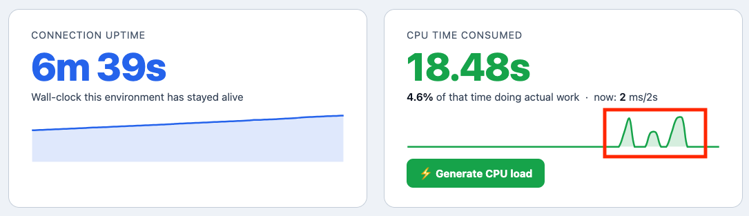
Figure 3: CPU chart mid-spike after choosing Generate CPU load.
For pricing details, read the AWS Lambda pricing page.
Concurrency and scale-out
With Web Functions, each execution environment handles many requests at once, not one at a time. As environments approach their concurrency limit, Lambda adds more environments and removes them again when traffic falls.
You can control how a Web Function scales. maxConcurrencyPerEnvironment sets the maximum number of requests each execution environment handles at once, up to 128, with a default of 64. On the endpoint, maxEnvironments caps the number of execution environments and rateLimit caps requests per second. You can use these two settings to protect downstream dependencies such as databases and external APIs. Both apply in each Region the endpoint serves and maxEnvironments applies to each revision. Requests above a limit receive HTTP 429 and are not queued.
Generate load on the app. Send 300 streaming requests to the /api/events endpoint, with up to 200 open at once, rather than a burst of quick responses.
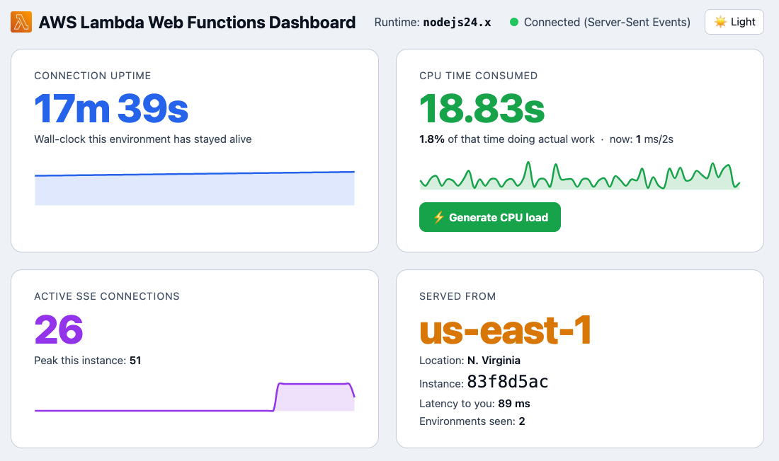
Figure 4: Concurrency showing increased connections in a single execution environment.
The dashboard updates to reflect the active SSE connections and peak for the currently connected execution environment.
The runtime also writes a per-environment summary record to Amazon CloudWatch Logs every minute with the instance ID, request count, peak concurrency, and CPU time. A CloudWatch Logs Insights query aggregates them across the fleet:
From a sample run of 300 streaming requests with up to 200 open at once, the logs showed the following:
- Execution environments used: 5.
- Total requests handled: 484.
- Peak concurrency on a single environment: 59.
- Total CPU consumed across the whole fleet: 4.75 seconds.
One environment peaked at 59 connections, near the default limit of 64. Lambda adds environments before existing ones reach their limit, so this load used five. Event Functions serve one request per environment, so 200 open streams would need up to 200 environments. Across 484 requests, the whole fleet used about 4.8 seconds of CPU.
Each environment reports only its own connections, because Lambda routes each request independently with no session affinity.
Going multi-Region
The same app can serve each caller from the Region with the lowest latency. Because an endpoint’s type and Regions are fixed when you create it, going global means adding a new endpoint:
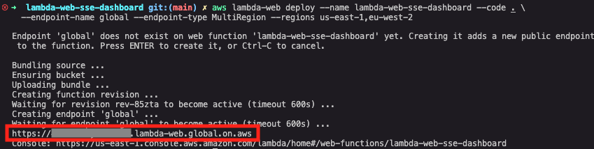
Figure 5: AWS CLI creating a global endpoint.
Lambda replicates your code and revision configuration, including environment variables, to each Region, and centralizes logs in the home Region. In this case, Lambda replicates to Europe (London) Region (eu-west-2). It provides a single global domain URL and uses Amazon Route 53 latency-based routing to send each request to the lowest-latency Region.
Browse to the new global URL which is now in the format: https://<domain>.lambda-web.global.on.aws
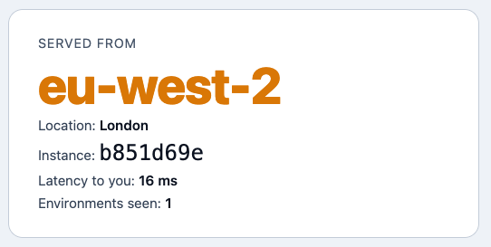
Figure 6: The app dashboard showing routing to the local Region.
From my laptop in the United Kingdom, the request routes to eu-west-2 (London) in 16 ms, where the single-Region endpoint in us-east-1 replied in 90 ms. These are single measurements from one location, not a benchmark. Each request goes to the Region with the lowest latency for the caller through the same URL. Lambda manages the DNS routing, so there are no load balancers or Route 53 records to configure.
Authentication and running behind Amazon CloudFront
Each endpoint has an authentication type that you can change without redeploying code.
With ApplicationManaged, the endpoint is public, and your code handles authentication (OAuth, JWT, a session cookie, or Amazon Cognito). Administrators can prevent public endpoints across an organization with a service control policy that uses the lambda:Request/WebFunctionAuthType condition key.
With IamAuth, Lambda validates each request with AWS Signature Version 4 (SigV4) for single-Region endpoints and SigV4a for multi-Region endpoints. Only callers with the lambda:InvokeWebFunctionEndpoint permission reach your app, which suits service-to-service APIs. Endpoints are always reachable over the public internet, and IamAuth controls who can invoke them.
Endpoints use a Lambda-provided domain. For a custom domain, edge caching, and AWS WAF, place Amazon CloudFront in front of the endpoint. Use IamAuth with origin access control so the Lambda domain cannot bypass CloudFront which still passes your application’s own Authorization header through to your code.
Build it with an agent
Because deployment is a single aws lambda-web deploy command and the code is an ordinary HTTP server, you can scaffold, build, and deploy an app from a prompt using AWS skills for coding agents. The Agent Toolkit for AWS includes Web Functions.
Clean up
To remove the default resources that the aws lambda-web deploy command created, see the cleanup instructions in the repo.
Conclusion
AWS Lambda Web Functions bring the serverless operating model to web applications without adapter layers. You write a standard Node.js HTTP server, deploy it with one command or CloudFormation, and get a scalable, pay-per-use HTTPS endpoint with global routing built in. Deploy the sample application from the Serverless Patterns collection along with other Web Functions patterns. Read the Lambda Web Functions documentation to go deeper and the Lambda roadmap.
For more serverless learning resources, visit Serverless Land.
[$] KDE Linux at two
Post Syndicated from jzb original https://lwn.net/Articles/1099486/
KDE Linux, the KDE Project’s second
stab at creating its own distribution, was first introduced as “Project Banana”
at the Akademy conference in 2024 by
Harald Sitter. Nate Graham announced
the first alpha-quality release during Akademy 2025. Graham and Sitter
paired up at Akademy 2026 to
provide an update on its progress, lay out plans for refining the distribution to
address user feedback, and discuss some of the problems that still need to be
dealt with. KDE Linux is still not-quite-ready for prime time, but Graham hopes
that it will be suitable for widespread use soon—for an undefined value of
“soon”.
Ivanti Connect Secure zero-day exploited in the wild (CVE-2026-104935)
Post Syndicated from Rapid7 original https://www.rapid7.com/blog/post/etr-ivanti-connect-secure-zero-day-exploited-in-the-wild-cve-2026-104935
Overview
On October 13, 2026, Ivanti published a security advisory for CVE-2026-104935, a high-severity authentication bypass by spoofing (CWE-290) affecting Ivanti Connect Secure (ICS). The vulnerability has a CVSSv3.0 score of 8.6 and allows a remote, unauthenticated attacker to execute arbitrary commands.
Ivanti reports that exploitation in the wild has already occurred prior to disclosure, affecting a limited number of customers. This indicates that exploitation has been occurring as a zero-day vulnerability. The U.S. Cybersecurity and Infrastructure Security Agency (CISA) confirms exploitation in the wild, and added CVE-2026-104935 to its Known Exploited Vulnerabilities (KEV) catalog on the same day as the vendor’s public disclosure. The digital forensics firm Volexity has published a detailed blog post describing the threat actor activity, which was detected in early October 2026. Volexity notes that in addition to leveraging CVE-2026-104935 as a zero-day, the threat actor also leveraged an as-yet unpatched privilege escalation vulnerability which Ivanti are planning to patch at a later date.
According to the vendor, a portion of the vulnerability was initially discovered through its product security program and patched in the July 2026 release of 25.1.3.0. Exploitation occurred while Ivanti was working to backport the fix to the remaining supported versions.
Ivanti Connect Secure is a popular enterprise VPN solution and naturally sits on the edge of a corporate environment. The product has a history of being targeted by attackers, with zero-day exploitation of other vulnerabilities occurring back in both 2024 and 2025.
Given the confirmed exploitation, the ability to execute commands without authentication, along with the history of the product, Rapid7 recommends that organizations running affected versions apply the appropriate update on an emergency basis outside of normal patching cycles.
Mitigation guidance
Vendor-supplied updates are available to remediate CVE-2026-104935. Ivanti lists the following affected and resolved versions:
|
Ivanti Connect Secure affected versions |
Resolved versions |
|---|---|
|
25.1.1.1 and prior in the applicable code line |
25.1.1.2 |
|
25.1.2.2 and prior in the applicable code line |
25.1.3.0, 25.1.3.1 |
|
22.8R2.4 and prior in the applicable code line |
22.8R2.5 |
Note that the vendor advisory confirms that versions 22.7.x and below are unaffected.
At the time of the advisory, Ivanti states that reliable indicators of compromise are not available, however Volexity have published several here. Rapid7 strongly recommends looking for signs of compromise even after the patch has been applied. Customers who suspect exploitation should follow the vendor’s recovery steps.
For the latest mitigation guidance, please refer to the vendor’s security advisory.
Rapid7 customers
Exposure Command, Vulnerability Management, and Nexpose
Exposure Command, Vulnerability Management, and Nexpose customers can assess exposure to CVE-2026-104935 with a vulnerability check expected to be available in the October 14 content release.
Updates
-
October 13, 2026: Initial publication.
Under the hood, off the hot path: How D1 scales to millions of databases
Post Syndicated from David Laban original https://blog.cloudflare.com/d1-control-plane/
Traditional database architecture assumes you have one or two big database clusters per application, usually accompanied by a connection pooling solution. AI-assisted development and vibe coding platforms turn this model inside out and are driving applications toward many small databases: one per user, application, preview environment, or tenant.
That model fits D1 particularly well. D1 is Cloudflare's managed, serverless database based on SQLite. It allows you to create millions of databases and only pay for what you use.
The question becomes: how do you scale the control plane for millions of databases without making every query slower by sending it through centralized bottlenecks?
We made a lot of architectural changes to scale out D1 to support platforms with millions of created databases, hundreds of thousands of which are active at any point.
This post is a behind-the-scenes deep dive into how the D1 control plane works. Many of the architectural patterns we will describe can be used by anyone building on top of Cloudflare’s Developer Platform. The post also gives a glimpse into how we build our own control planes.
Growth in numbers
There was already a steady growth in D1 usage when we started planning these changes, but we knew we would need to support a much bigger scale once large platforms started building with D1.
Here is how things have played out so far.
D1 has seen a 15x growth in the number of live non-deleted databases over the past one year, and a 65x growth over the past 2 years (as of October 8, 2026).
We have also seen 18x growth in the number of daily active databases over the past year (as of October 8, 2026). A database is considered active if it executed at least one query during that day.
Established and successful platforms are already building with D1, using the same tools available to all Cloudflare users.
"ChatGPT Sites lets anyone turn ideas into shareable experiences. D1 gives our users a simple, scalable way to add features like custom metrics, leaderboards, and comments to their dashboards, games, and tools."
– Jon Abrams, ChatGPT Sites @ OpenAI
While we were making the changes described in this blog post, we periodically load-tested against a target well above our expected growth. This guided where to focus our optimization efforts.
Guiding engineering principles
Applications built on the Cloudflare Developer Platform range from full-stack applications to service APIs, from internal single-user portals to massive multi-tenant vibe coding platforms, and everything in between.
While building out the D1 control plane to support millions of databases, the following tenets and principles were guiding our architecture decisions and are useful for anyone building their control and data planes on our platform.
- Design all processes with failure and idempotency in mind. Failures will happen, so the system needs to self-correct where possible and continue making progress.
- Avoid centralized single-region components in any hot path for data plane operations (in our case all query requests).
- Use Workers KV, a globally distributed KV store, for critical routing metadata so that cache misses only rarely need to query central databases.
- Use Hyperdrive to access central Postgres databases for efficient connection pooling and optimized routing and caching, using read replicas wherever possible.
- Periodically precompute aggregations in the database to avoid scan queries during user request processing.
- Use eventual consistency and queuing between components that don’t need strong consistency to increase reliability and availability.
- Load-test the application with realistic workloads to discover bottlenecks and inefficiencies, and focus on optimizing those first.
There are more engineering principles we follow internally to build our systems, but the above are generic enough and apply to anyone building on Cloudflare.
The following sections will dive into the main system components and processes of the D1 control plane regarding the lifecycle of a D1 database, and showcase how to put these principles into practice with a real-world system.
High-level architecture
Let’s start off by introducing the main components of D1.
There are a few more arrows and boxes missing from the diagram for secondary processes supporting D1, but these are the ones providing D1’s public feature set. We will explore the rest in dedicated sections in the rest of the blog post.
First of all, each D1 database is backed by one SQLite Durable Object, which makes it very easy to create millions of them.
The “HTTP API” shape represents all our API surfaces including the Cloudflare dashboard, Wrangler, and Cloudflare CLI. All API requests go through Cloudflare’s edge gateway and are served by the D1 Edge API Worker.
The diagram shows the HTTP endpoints that allow users to execute SQL queries against their databases as the “Query endpoints”. The remaining endpoints include the usual database operations like creating, deleting, and listing databases, along with import/export and time travel features. These are shown as the “CRUD endpoints”.
The CRUD endpoints use Hyperdrive to query a Postgres cluster in our central data centers (referred to as “Core”). There are two configurations. One configuration has caching enabled and targets the Postgres read replicas. The other configuration has caching disabled and targets the Postgres primary.
The Edge API Worker might invoke the D1 Eyeball Worker (depending on the type of request). The Eyeball Worker is our proxy for all requests that need to be handled by the underlying D1 Durable Objects (DO). This allows us to put all query handling inside the Eyeball Worker, including observability, automatic retries, error handling, and other query-specific behaviors.
Workers KV acts as our caching layer at the edge for read-heavy metadata and can be read by all the D1 Workers.
The “Worker Binding” shape represents all users’ Workers with a D1 Worker binding. Requests from the D1 Binding go directly to the D1 Eyeball Worker, which in turn forwards the request to the Durable Object backing the database and proxies the response back to the User Worker.
We have two methods for users to execute queries in their databases. One is over the HTTP API query endpoints, and the other is through a Worker they deploy in their accounts with a D1 Binding.
In terms of operations, we fold each operation into one of the following categories:
- Data plane: any database query related request; should be as fast as possible and always at the edge.
- Control plane: any HTTP API operation or internal flows that run in response to a non-query user request; they can depend on central single-region components.
- Background asynchronous plane: any analytical and billing-related workflow; can be eventually consistent and runs anywhere.
There is a lot more under the hood, so let’s dive into the key flows.
Fast on-demand database creation close to the user
Multi-tenant platforms and AI agent-driven development require creating a lot of database instances in a fast, cost-efficient, and reliable way.
The following is an example Wrangler command to create a D1 database:
% time wrangler d1 create "demo-01"

✅ Successfully created DB 'demo-01' in region WEUR
...
0.56s user 0.13s system 42% cpu 1.614 total
When a user creates a D1 database, several things need to happen before the database is ready to receive queries.
- Check that the account can create more databases against the free tier limit or its account limits.
- Generate a unique D1 database UUID, a unique Durable Object ID (
newUniqueId()), and initialize the underlying Durable Object (DO) with the account and database information. - Persist the newly created database’s information in Postgres (one row per database, including metadata and the mapping to the initialized Durable Object ID).
- Write the mapping from a database ID to the Durable Object ID in Workers KV (later used by the data plane and the query endpoints).
Let’s examine the actual flow and how we recover from failures at each step.
Once a database creation request comes in, our Edge API Worker handler is invoked in the nearest Cloudflare location at the edge. Edge API queries our Postgres read replicas over Hyperdrive with caching enabled (with cache TTL of a few seconds) to get the number of non-deleted databases for the given account.
The Edge API Worker forwards control plane requests to data centers near our Postgres cluster for endpoints that do multiple round-trips to Postgres (step 2), and the “create database” endpoint is one of them. The reason is that a round-trip from afar can be hundreds of milliseconds, whereas being near Postgres can be a few milliseconds. For endpoints that do at most one Postgres query we don’t need to do this optimization since Hyperdrive already handles efficient routing through the Cloudflare network.
Creating a D1 database without any options places the database near the request’s location by default. You can influence the location of the database by providing an explicit location hint or a jurisdiction. The location hints and jurisdiction options are identical to what Durable Objects support, so when these are provided they are just passed straight through to the underlying Durable Object initialization.
With the default creation we want the D1 databases to be created near the original location of the request, close to the user. To achieve this, during step 4 of the diagram, we internally forward the request execution to a data center close to the original request’s location and invoke the underlying Durable Object from there. This ensures that the underlying Durable Object is placed near the user.
You can implement similar routing techniques by using explicit Worker placement hints and at runtime invoking the right Worker via Service Bindings.
The creation endpoint is a bit of a weird case in terms of placement because even though we query Postgres at least two times, we also do a long-distance call to the underlying Durable Objects, which differ per request, so running the request to either side of the world could be inefficient. That's why we leaned towards forwarding the initial request near Postgres.
The next step is to generate the database UUID along with a new unique Durable Object ID using the newUniqueId() API and invoke the init(options) RPC function on the new Durable Object’s stub. The Durable Object stores the information in its durable storage so that every incoming request from that point on has all the metadata for the linked database.
Once the Edge API Worker gets the initialization response, it persists the database metadata into our central Postgres primary database over Hyperdrive, one metadata row per database.
The steps above are wrapped in a retry loop (steps 5-7 in the diagram). When the DO initialization or the write to Postgres fails we retry with different IDs (this is important, as we will see in the next section).
The write to Postgres is the “creation checkpoint” where a database is considered created even if the final response fails to reach the user. The database from that point on is included in all the control plane operations and can be bound to a Worker to serve queries.
At this point the D1 database is ready to receive queries.
The final creation confirmation RPC to the Durable Object happens in a waitUntil() and is OK to fail. This call signals the DO that the database is now active, and the DO updates Workers KV with the database metadata so that any subsequent query can immediately read the information from Workers KV cache without needing to query Postgres.
A common question is why can’t the creation flow run entirely inside a Postgres transaction to simplify the process? The answer is simply that it cannot scale, since it leads to connections being held while the Durable Object is being initialized, which could be on the other side of the world.
Heartbeats for self-correcting databases
Each D1 Durable Object periodically heartbeats the control plane to get the latest database state (active or deleted) and account limits (more on this in the enforcement sections later). The interval is 30 seconds with a per-database jitter on top. We also have knobs to change the interval by database or account, or disable heartbeats entirely.
Heartbeats can tolerate slightly out-of-date data, meaning they can be served by Hyperdrive’s multiple caching layers or by a Postgres read replica. This heartbeat flow enables the Durable Object to self-correct to reflect the source of truth (Postgres) regarding the creation and deletion of databases.
One clarifying detail before we move on. The reason we use different database UUID and Durable Object IDs for each retry in the creation flow of the previous section (step 5) is that if we reused the database UUIDs with fresh Durable Object IDs, multiple Durable Objects would think they own the same database leading to difficult-to-debug situations. The periodic heartbeats also act as a cleanup for orphaned objects.
Also, it’s important that we first initialize the Durable Object before we persist the database mapping in Postgres, otherwise query requests could start to flow to the Durable Object and would be rejected due to uninitialized state.
For example, let’s assume the following failure scenario and why it is self-correcting:
- We executed everything from the previous section until we initialized Durable Object A, and then, the write to Postgres fails.
- The Worker retries the loop and initializes a new DO with a different ID B, and this time it persists to Postgres.
- We now have two Durable Objects initialized and running as part of this request, but only one of them is valid.
- The user can only query Durable Object B because that’s the only ID available in Postgres, which is our source of truth.
- Within 30 seconds, DO A sends its next heartbeat to the control plane and receives back a response that its database does not exist. This will trigger DO A to mark itself as deleted.
A similar flow happens for the deletion endpoint.
Another self-correcting behavior of the heartbeats is making sure the Workers KV data eventually reflects reality: whether a database is active or deleted.
The final step of the creation flow to update Workers KV is “best-effort” and can fail without causing problems. It’s eventually consistent, and the next time the Durable Object heartbeats it will ensure that the Workers KV item has been written with the correct value. Since Workers KV is eventually consistent without a way to do a consistent read, the Durable Object acts as the serialization point for the writes to the Workers KV items.
Deletion works the same way in reverse: the Durable Object owns writing its “deleted” state to Workers KV, again best-effort during the actual deletion operation, and if that fails the heartbeat will correct it eventually. The Durable Object stores the active or deleted state in its storage too, so it can reject or accept query requests immediately, even if Workers KV is stale and allows requests through.
Overall, the database heartbeats are the fallback mechanism for getting into a consistent state when operations need to write into an external datastore and also update the Durable Object itself.
Decoupling the hot path: keeping queries off the central database
The key principle for query endpoints is to avoid talking to Postgres or any other centralized single-region component. Each query request over HTTP executes our Edge API Worker close to the original user request location, and then goes straight to the D1 Durable Object via the Eyeball Worker.
The Edge API Worker is responsible for doing standard HTTP API authentication, resource-based authorization, rate limiting at the account and database level, request validation, checking the entitlements of the account, and other API-related functions before executing the actual business logic.
The Eyeball Worker, on the other hand, skips these extra checks (apart from its own dedicated rate limiting), since under the hood, a D1 Binding is a Service Binding to the D1 Eyeball Worker. Each user Worker’s D1 Binding carries encoded information that authorizes access to one specific D1 database that the D1 Eyeball Worker validates and allows the request through.
The following diagram shows the execution of a query through the HTTP API.
- A user sends a query request over the HTTP API.
- The Edge API Worker first tries to load the mapping from a D1 UUID to the database metadata from Workers KV.
- In rare cases, the item cannot be found in Workers KV, either because the write failed as described earlier or potentially due to an availability issue. We then fall back to reading the mapping from Hyperdrive targeting the Postgres replicas. Before querying the actual replicas, Hyperdrive first checks its cache in the caller location, then its cache near the Postgres cluster location, and only if both are cache misses queries the Postgres replicas for the mapping.
- Once we have the mapping, the Edge API Worker calls the Eyeball Worker over Worker Service Bindings passing the relevant IDs.
- The Eyeball Worker does its validation and forwards the query request to the D1 Durable Object.
- The D1 Durable Object executes the SQL query and returns the result through Eyeball Worker to the Edge API Worker, which returns it back to the user.
// Edge API Worker
const parsed = parseQueries(request);

const cachedDB = await withRetries(getCachedDatabase(parsed.dbUuid));

const response = await env.EYEBALL_WORKER.query({
  db: cachedDB,
  queries: parsed.queries,
});

return response;
If you are wondering why we use newUniqueId() during the database creation rather than addressing Durable Objects by “name” to eliminate steps 2 and 3 above, the answer is to avoid a lookup round-trip to a central mapping of “name” to “Durable Object ID” during query requests. The Durable Object ID alone would not be enough, since we also need other metadata to help us pick the right Durable Object Namespace to use in our Eyeball Worker. Hence, we would replace one lookup with two.
In most cases, even with many of our own applications, addressing Durable Objects by name works great, and it removes the need for a lookup from your own IDs to a Durable Object ID, so use that as a starting point and only move to unique DO IDs if you have to.
You might also wonder why we use Workers KV when we already have Hyperdrive Caching.
Workers KV is a durable datastore, not just a cache: if an item falls out of KV's edge cache, the read is served from KV's own storage rather than Postgres, keeping Postgres out of the data plane. In a catastrophic cache purge scenario, a million databases trying to fetch their routing information would lead to metastable failures.
As a reminder, query requests from a user Worker with a D1 Binding do not need to resolve the D1 UUID mapping metadata because the binding itself holds that information internally, so requests go straight to the Eyeball Worker and the Durable Object.
For the query execution itself and how Durable Objects are implemented under the hood, read our blog post about D1 read replication that dives into all the nitty-gritty details.
Next, let's look at the asynchronous processes that support D1.
Enforcing storage usage limits
All platforms that reach a certain scale eventually need to enforce billing and usage limits. At the time of writing, D1 has a 5 GB per-account storage limit on the Free plan and 1 TB on Workers Paid (can be raised on request).
In general, usage limit enforcement and billing systems are good candidates for eventual consistency and asynchronous processing, and in the following sections we will explore how D1 implements the enforcement of these limits.
Asynchronous update processing with queues
The first step of the journey is that each Durable Object publishes storage usage updates to a Kafka-like queue for batching and asynchronous processing. The control plane does not need to process every update synchronously: it is fine if a load spike is not reflected immediately and our usage information is stale. The important thing is that it cannot overload Postgres and impact users of D1. We ensure this by limiting the number of queue consumers, and therefore the write load on Postgres.
The queue consumer system runs inside Cloudflare’s central data centers (“Core”), whereas the Durable Objects themselves are spread everywhere in the world at the edge. The usage is aggregated locally per edge server and then published into the internal queue system.
The guiding principle here is that we use a queue to smooth out and batch writes to our central regional Postgres data store.
Batching usage deltas and pre-aggregations
The queue consumer writes the latest reported size for each database into a Postgres table. This isn’t what we need for enforcement decisions though. For enforcement decisions, we need the sum of all storage usage across the whole account. When we come to read the usage at enforcement time, we can’t afford to run SELECT sum(storage) FROM database_stats WHERE account_id = ?. The cost of this query scales linearly with the number of databases on each account. This doesn’t scale for accounts with millions of D1 databases, like some of the agentic coding platforms built with D1.
Ideally, we want a lookup table that will allow us to go directly from account ID to total database storage. The solution is to use incremental view maintenance to precompute the total, and keep it up to date when we have database storage changes.
Let’s call this table account_database_stats.
In theory, we could make the queue consumer update database_stats and account_database_stats itself for every update that comes in. In practice, this would end up with a lot of write lock contention on a single row for large accounts. Instead, we add a third table called account_database_stats_changes that acts like a queue of changes. This is a log of all changes, and can have multiple entries per account. We then periodically aggregate updates from that table into account_database_stats. The flow looks like this:
- The queue consumer writes usage info to the
database_statstable for a specific database. - A trigger calculates the difference in storage for that database and puts the delta in an
account_database_stats_changestable (one row per delta). - A scheduled job runs every second to consume everything in
account_database_stats_changesand updateaccount_database_statswith the sum of those deltas.
Concretely, the scheduled job runs this query:
WITH updates AS MATERIALIZED (
  DELETE FROM account_database_stats_changes
  RETURNING *
),
changes AS MATERIALIZED (
  SELECT
    account_id,
    SUM(storage_change) AS storage
  FROM updates
  GROUP BY account_id
)
INSERT INTO account_database_stats (account_id, storage)
SELECT
  account_id,
  storage
FROM changes
ON CONFLICT (account_id) DO UPDATE
SET storage = account_database_stats.storage + EXCLUDED.storage;
It gets a list of updates from account_database_stats_changes, aggregates them by account, and then writes the deltas to the per-account table. This avoids write contention on any particular row, because we aggregate the changes before writing them.
The Common Table Expression (CTE) DELETE ... RETURNING atomically consumes the pending changes and passes the deleted rows to the next CTE. Postgres executes the data-modifying CTE exactly once and to completion. The query then groups those changes by account and applies one aggregated update per account, reducing write contention.
This schema design is a pattern used by many other Cloudflare teams, and it lets us scale to millions of resources per account without each additional resource making common operations more expensive.
It’s worth noting that the total is eventually consistent. It’s not like first-class incremental view maintenance that you find in some other databases. We are already using a queue to get the updates from the Durable Objects into Postgres, so we are already fine with eventual consistency.
Cached reads via Hyperdrive
We now have a lookup table for each account’s total storage. What next?
Each D1 Durable Object periodically retrieves the account’s usage through the periodic heartbeat we mentioned earlier. We query Postgres with SELECT storage FROM account_database_stats WHERE account_id = ? and compare that to the account’s entitlement and tier limits. If the total is over the limit then we forbid all writes that would increase the database size.
The query goes to Postgres replicas through Hyperdrive, and uses Hyperdrive’s built-in cache. Hyperdrive’s cache key is made up of the query and all parameter values, with the expiration time-to-live being a few seconds. By using the account ID as the only parameter, every database on that account will share the same cached value, which is what we want.
Time for a neat cache trick. Cached reads via Hyperdrive by default have a 60s expiration, and the Hyperdrive cache configuration applies to all queries. For specific queries we want cached values with lower expiration time. By adding a dynamic_ttl parameter to the query we generate a different cache key every X seconds, therefore reading fresh values sooner.
-- $2 = Math.floor(Date.now() / (X * 1000))
SELECT storage, $2 as dynamic_ttl
FROM account_database_stats WHERE account_id = $1
It might be tempting to make a query that takes account ID and database ID as parameters. That would let you find the account total and subtract the total for the current database. That would get an exact answer to the question “how much storage is this database allowed to use before we start enforcing?”, which would allow the database to start enforcing limits earlier.
Doing this would mean that the database ID would be included in Hyperdrive’s cache key, which would make cache hit rates very poor. For accounts with millions of active databases, an account-based cache key means that most of the heartbeats use the same cached account information from Hyperdrive and never reach Postgres.
Limit enforcement is slightly slower than it could be in terms of reaction to usage changes, but this is acceptable.
Separately from the above flow, we have a process that periodically snapshots the storage usage information from Postgres into a ClickHouse cluster, so that we can get a historical view of storage over time. These ClickHouse events are also the source of truth for storage usage billing purposes.
Enforcing row usage limits at the edge
D1 also enforces daily execution usage limits for free tier customers. The pattern we use here is different, and is worth mentioning as well.
Whenever an SQL query is executed in a Durable Object, we track how many rows it reads and writes (including index updates if needed) to perform the query. When the query execution completes, we publish a usage event that ends up in another ClickHouse cluster. These events are what drive our row-based usage billing.
A central component, call it “Limiter”, runs in our Core data centers and periodically queries the usage events from ClickHouse since the start of the day:
SELECT account_id, sum(rows_read) as reads, sum(rows_written) as writes
FROM requests
WHERE timestamp > toStartOfDay(now())
GROUP BY account_id HAVING reads > ? or writes > ?
ClickHouse deals with this kind of query better than Postgres, and we also benefit from not overloading our Postgres cluster for analytical queries.
For every account that is over the limit, we check their entitlements and tier (this limit applies only to free tier users). If they are over a limit, we email them (deduplicated throughout the day), and set a key in Quicksilver, our internal globally distributed key-value store with fast sub-second replication, with an expiry date at the end of the day. If the account upgrades to the Workers Paid tier, we receive a message on a queue and clear the Quicksilver key.
Each D1 Durable Object periodically checks Quicksilver at the edge to find out whether its account has been limited, and in case it is, they reject any future query execution until the limit is lifted.
Someone building on the Developer Platform can use Workers KV Instant, which is built on top of Quicksilver.
This pattern avoids any load into the regional Postgres for the entire flow and uses the right tool for the right job. Doing analytics queries with ClickHouse is more efficient than doing them in Postgres.
This pattern is common across the company, but different from the approach we use for storage usage limit enforcement. In the future, we may migrate other limit enforcements to use this pattern instead.
Conclusion
The D1 architecture is designed around separating control plane concerns from hot-path query execution.
Each decision follows our guiding principles: reducing central regional bottlenecks, using caching and read replicas along with eventual consistency when possible to scale out read throughput, and choosing the right data store for each job: Postgres for transactional metadata, ClickHouse for analytics, and Workers KV for globally replicated routing data.
If you are building a vibe coding platform and want to offer your users managed SQLite databases in a fast, cost-efficient, and reliable way, consider using D1.
If you are building applications on Workers and the Developer Platform, the patterns and trade-offs covered here reflect real decisions made for D1. Use them as a foundation in your own applications.
Check out the D1 documentation, and let us know what you build in the D1 Discord channel!
Acknowledgements
Massive thanks to Cloudflare’s internal Databases and Hyperdrive teams, who helped us find problematic usage patterns and suggested improvements.
Nix and Lix local root-privilege-escalation vulnerabilities
Post Syndicated from jzb original https://lwn.net/Articles/1100247/
The Lix and Nix projects have jointly
disclosed a set of vulnerabilities that can be used to escalate privileges
to root on systems running the Lix or Nix daemons. “All systems that build
” Releases with fixes from each project
untrusted derivations are affected.
are available today. CVE IDs have not yet been requested. See the announcement
for more details on the vulnerabilities.
Your Smart TV Is Spying On You – Here’s How to Lock It Down
Post Syndicated from Crosstalk Solutions original https://www.youtube.com/watch?v=DyTDMEIqKe0
Alexis Nikole Nelson | Happy Snacking, Don’t Die! | Talks at Google
Post Syndicated from Talks at Google original https://www.youtube.com/watch?v=lHai_qaI3HI
Sony A7R6 VS Medium Format
Post Syndicated from Matt Granger original https://www.youtube.com/shorts/7DeEQHQ3C-Y
AWS Weekly Roundup: Prime Day 2026 by the numbers, Claude Haiku 5.5, Amazon Nova 2.5 Sonic, and more (October 13, 2026)
Post Syndicated from Daniel Abib original https://aws.amazon.com/blogs/aws/aws-weekly-roundup-prime-day-2026-by-the-numbers-claude-haiku-5-5-amazon-nova-2-5-sonic-and-more-october-13-2026/
Some numbers are hard to picture until you sit with them for a moment. Last week we published the Prime Day 2026 metrics, and the one that stuck with me is 2.3 quadrillion: the daily requests Amazon ElastiCache peaked at during the event. Prime Day ran back in June, so this post always lands as a retrospective, and that gap is part of what makes it worth reading. By the time the numbers reach you, the only evidence that any of it happened is that nothing went wrong.
The rest of the week pulled in a different direction: smaller, cheaper, and more constrained. Claude Haiku 5.5 arrived on Amazon Bedrock at roughly 75 percent less than Haiku 4.5, Amazon Nova 2.5 Sonic made voice agents quicker on their feet, and Strands Box showed up to put real boundaries around what an agent is allowed to do. Now, let’s get into this week’s AWS news…
Headlines
All the numbers: Amazon Prime Day 2026 powered by AWS is the latest entry in a tradition that goes back to 2016, and the scale is still difficult to hold in your head. Over the four days of Prime Day, Amazon DynamoDB processed more than 59 trillion requests while peaking at 192 million requests per second, and kept single-digit millisecond responses throughout. AWS Lambda handled over 2.3 trillion invocations per day. Amazon EBS peaked above 24.8 trillion I/O operations, moving more than an exabyte of data daily. Amazon ECS launched an average of 158.3 million tasks per day on AWS Fargate, a 47.7 percent jump over last year, and AWS Graviton powered up to 49 percent of the Amazon EC2 compute that Amazon.com used.
The number I keep coming back to, though, isn’t a throughput record. The team ran more than 44,000 AWS Fault Injection Service experiments ahead of the event, more than six times what they ran in 2025. Those are deliberate failures injected on purpose, months in advance, so that the trillions of requests above turn into an ordinary shopping afternoon. If you’re preparing for your own peak moment, AWS Countdown Premium is built for exactly that kind of planning.
Last week’s launches
Here are some launches and updates from this past week that caught my attention:
- Claude Haiku 5.5 is now available on AWS – You can now use the fastest model in the Claude 5.5 family on Amazon Bedrock and Claude Platform on AWS, at around 75 percent less than Claude Haiku 4.5 for most tasks. It’s the first Haiku with effort controls, so you can tune cost against intelligence per task instead of fixing one setting for a whole workload. It pairs naturally with Claude Opus 5.5: Opus plans and makes the judgment calls, and because Haiku is fast and cheap, you can run many Haiku subagents in parallel for routing, classification, and small code changes across many files.
- Amazon Nova 2.5 Sonic for voice agents – You can now build real-time voice agents on a speech-to-speech Amazon Nova model with better reasoning, instruction following, and tool-calling accuracy, plus lower latency. That combination matters for multi-step work: a support agent can look up an order, check return eligibility, and start the return inside one conversation. It keeps expressive voices in seven languages, controllable turn-taking, and a 256K context window, and pairs with Strands Bidi Agents, now generally available, to get a production voice agent going in a few lines of code.
- Amazon GuardDuty RDS Protection now detects data exfiltration and destruction – Amazon GuardDuty now looks past login anomalies to the queries themselves on Amazon Aurora PostgreSQL and Amazon RDS for PostgreSQL. RDS Protection for data activity builds behavioral baselines and uses ML-based anomaly detection plus threat intelligence to flag unusual data access, with no agents, extra infrastructure, or database configuration changes. This closes a real gap: once an attacker has valid credentials from phishing or a misconfiguration, their queries can look indistinguishable from your application’s.
- AWS Lambda supports OAuth for self-managed Apache Kafka event sources – You can now authenticate Lambda Kafka consumers through your enterprise identity provider, such as Amazon Cognito or Okta. Event source mappings previously supported only SASL/PLAIN, SASL/SCRAM, and mTLS, which left teams in regulated industries unable to use Kafka ESM at all. Now you get the automatic scaling, batching, error handling, and event filtering of Kafka ESM with the same identity governance you apply everywhere else. It works with self-hosted clusters and managed offerings including Confluent Cloud, Aiven, and Redpanda.
- Amazon Redshift adds Apache Iceberg materialized views – You can now pre-compute expensive joins and aggregations once in Amazon Redshift and store the result as an Iceberg table in Amazon S3, registered in the AWS Glue Data Catalog. You create them with familiar SQL, and the results are immediately queryable by any Iceberg-compatible engine, including Amazon Athena, Apache Spark, Trino, and Snowflake. Redshift keeps them current by recomputing only what changed. There’s a good deep dive on the AWS Big Data blog if you want the details.
For a full list of AWS announcements, be sure to keep an eye on the What’s New with AWS page.
Other AWS news
Here are some additional posts and resources that you might find interesting:
- Introducing Strands Box: AI agent sandboxes powered by Dogwood – As more of us let agents run shell commands and call APIs without approving every step, isolation alone stops being enough. Strands Box is an open source sandbox (Apache 2.0, developer preview) that combines OS-level containment with fine-grained policies written in Dogwood, so permissions can depend on what the agent has already done. You can say “let the agent post to the incident channel, but no more than three times every 10 minutes” and have that enforced from outside the agent’s process. It also keeps real credentials out of the agent’s environment by attaching them at an egress gateway.
- AWS Continuum sets a new standard in autonomous code security – Related to that theme, AWS Continuum for Penetration Testing now integrates into your CI/CD pipeline in public preview, turning penetration testing into a deploy-time event instead of something that happens off to the side. Developers get findings with severity, affected endpoints, and remediation guidance right in the pipeline output, and the pipeline re-tests to verify fixes.
- How Postman runs Agent Mode for 40 million developers on Amazon Bedrock – A look at the architecture behind a feature serving a very large developer audience. Worth reading if you’re moving an agentic feature from a demo to something that has to hold up under real traffic.
- ICYMI: What landed for AI builders in September 2026 – If you lost track of a month that included a lot of model launches, this is a tidy catch-up in one place.
Upcoming AWS events
Check your calendar and sign up for upcoming AWS events:
- AWS re:Invent – re:Invent returns to Las Vegas from November 30 to December 4, and reserved seating is now open. The session catalog is live, so register and claim your spots in chalk talks, workshops, and builders’ sessions before they fill up.
- AWS Community Days – Community-led conferences planned and delivered by community leaders, and this is a busy stretch. Upcoming stops include San Francisco (October 13), Miami (October 14), Brisbane (October 16), Cape Town (October 16), Malta (October 16), and Mumbai (October 17). Here in Brazil, the community calendar has more editions coming before the end of the year.
Join the AWS Builder Center to connect with builders, share solutions, and access content that supports your development. Browse here for upcoming AWS-led in-person and virtual events and developer-focused events.
That’s all for this week. Check back next Monday for another Weekly Roundup!
– Daniel Abib
This post is part of our Weekly Roundup series. Check back each week for a quick roundup of interesting news and announcements from AWS!
Rewinding the exponential: How we keep hardware usage down
Post Syndicated from Cathy Chi original https://blog.cloudflare.com/rewinding-the-exponential/
More than 20% of the web sits behind Cloudflare’s network, and our team, the Data team, owns the data pipeline responsible for plumbing that data (and more) from our global network to applicable central data centers. The Cloudflare network is a globally distributed system supporting tens of thousands of servers. Data that power Cloudflare Logs, SQL API, observability, internal analytics, and more flow through this network and use our data pipeline to serve customers.
In May of this year, we were providing data delivery at roughly two billion events per second. This includes customer traffic as well as data sent from internal teams. Year after year, we tackle the same problem — exponential traffic growth against linear hardware growth. We have to react to this increase in order to keep resource costs under control. Over the past five years, we’ve made various improvements to compensate for the data volume increase in comparison to hardware allocation, equivalent to deferring two and a half years of hardware expansion. This post details those changes: breaking up our monolithic data schema in 2022, adjusting compression in 2024, rearchitecting pipeline replication in spring 2026, decentralizing sampling in summer 2026, and introducing aggregations into the pipeline in fall 2026.
Background
Our pipeline starts with an internal service called Logfwdr, where we collect from highly distributed data sources (think: Workers, FL). We then feed this data to a set of centralized receivers, which eventually push them onto our buffering system, Buftee. Consumers fetch data from Buftee and distribute data to their final destinations, like ClickHouse, which we rely on heavily.
Unpacking the monolith
In 2022, we dismantled our one and only schema. Previously, there was a single stream packed with every product's fields, forcing Cloudflare-internal consumers to ingest everything and demux or discard records via filters. At the time, most of Cloudflare’s data products were built on HTTP, Security and CDN metadata. In 2021, our message schema looked like this:
Some fields here belonged under the same product, but some were completely irrelevant to each other. The hypothesis was that none of these teams require 100% of fields in the monolithic schema. In other words, we can create small messages for each product’s required fields. Although we were going to duplicate fields, some of them in every message, replacing this firehose with product-specific schemas actually reduced the backbone bandwidth usage by 35-40%, knocking out roughly a year’s worth of compressed traffic growth.
Compression
By 2024, as traffic steadily grew, we were tackling network congestion issues on a daily basis. To react to this, we changed our compression algorithm from LZ4 to zstd. We had already experimented with zstd compression before, but we noticed a higher CPU usage at the time. Therefore, we were careful to track the metrics to ensure the trade-off was worth it.
Initially, we rolled this change out to a few servers. To our relief, we didn’t observe a noticeable difference in CPU usage.
With more confidence, we gradually rolled out to our entire fleet, which also showed little impact to CPUs. In the end, there was nearly a 40% reduction in compressed traffic throughput. The uncompressed bytes remained at the same growth, meaning we could support more than 1.5x the amount of traffic with the same size pipe. Or another way to put it, the estimated growth-equivalent reductions put us at about 10 months prior.
Now, in 2026, we attempted three strategies to reduce uncompressed bytes (and thus, compressed bytes).
Load balancing
To make analytics resilient against regional disasters, our systems require redundant data to be stored in multiple centralized regions (data subject to Customer Metadata Boundaries is stored strictly within its designated region). Historically, the simplest way to achieve disaster resilience was double-writing: Logfwdr transmitted two full copies of every non-regional analytics event — one to each centralized region. Each region then independently processed a complete copy through to ClickHouse. We also apply sampling in each region, an incredibly scalable technique that works for all volumes of data during any traffic conditions. We downsample high-volume traffic while rare events are preserved.
This infrastructure was manageable when only a handful of streams used secondary regions. However, as we expanded disaster resilience across almost all analytics streams, Logfwdr traffic doubled across the board. Sending every event, twice, over wide-area transit was unsustainable against our exponential traffic growth.
We had already tackled a similar challenge for Logpush. For Logpush, Logfwdr treats the centralized data centers as a unified, shared pool of receivers: each message is sent to only one region, failing over to another destination if a machine or facility is unreachable. That model had already proven its worth during large incidents, shifting traffic seamlessly from one location to another without human intervention. This automatic failover was possible because Logpush delivery is stateless, as customer destinations do not care which centralized data center pushes the logs.
Analytics was trickier. Unlike stateless logs, ClickHouse clusters in both regions still need a full copy of non-regional data to allow instant, independent query failover. The breakthrough was decoupling pipeline transit from database redundancy:
1. Shared Ingest Pool: We adopted Logpush’s model to the analytics streams. Logfwdr dispatches each event exactly once across wide-area transit to whichever centralized receiver is available.
2. Late Replication from centralized regions: Instead of replicating traffic at source, replication happens as late as possible in the pipeline. Data lands in our distributed buffering layer, Buftee, and remote inserters stream cross-data-center copies downstream.
3. Resilient Failure Handling: If a centralized region goes down, Logfwdrs immediately routes all non-regional traffic to the surviving region. If the inter-data center connection blips, each cluster continues ingesting its local share without backpressure; remote inserters catch up from Buftee's retention buffer once the backbone recovers.
For the datasets we migrated, the cutover eliminated approximately 43 GB/s of compressed transit traffic while adding only ~7 GB/s of cross-data-center replication on our pipeline. Two architectural factors explain this asymmetry:
1. Replication happens downstream of sampling: In the old model, Logfwdrs transmitted two copies of raw, unsampled events over wide-area transit. In the new model, Logfwdrs send a single copy to centralized receivers, which immediately apply sampling before buffering into Buftee, carrying only this already-compacted stream.
2. Better compression through uniform partitioning: Data at source is fragmented across thousands of individual servers. After centralization, streams are aggregated and partitioned into uniform batches over wider time windows. This structural uniformity allows compression algorithms to achieve dramatically higher compression ratios than Logfwdr transit batches ever could.
Overall, this was a net reduction of 36 GB/s across wide-area networks. We rolled this out initially to two datasets, HTTP analytics and Ready-Analytics, our in-house one-click analytics product.
We’ve been actively migrating more datasets to this load-balanced architecture since the spring.
Sampling from the get-go
Another strategy we employed was further expanding our sampling mechanism so that we pulled critical processing earlier into the pipeline. Sampling was already used in our centralized services, particularly the receivers, easing pressure on downstream systems. We can be more resource efficient if we send less data downstream (without sacrificing data quality).
The solution here was to simply sample in Logfwdr, in addition to maintaining the sampling in centralized receivers. How the sampling algorithm works here, in short, is each dataset has a key that producer teams have chosen to index and sample the data. When sampling, we first shuffle the records for each key to eliminate bias. Then, for each group of records, we select a sample size equal to the square root of the total count of the records. The result is a representative sample, whether sampled once or twice. To produce estimates, we scale calculations against the sample rate. For example, if we sample 10 out of 100 records, the sample rate would be 10/100, and the unbiased estimate of the original count would be 10*10 = 100.
To ensure this approach was working well, we compared the number of rows written to ClickHouse against the estimated sum for total count using a variety of keys across a variety of traffic footprints, so that “least seen” keys to “most seen” keys were captured across the spectrum.
The result is that for keys with more data, the sample rate decreases. However, keys with less data were sampled comparably. Thus, we still kept a representative sample while delivering and storing fewer events. We’re not compromising the quality of data delivered, even when we deliver less in quantity.
If we look at this more closely, using power laws, we can observe that the double-sampled (red) grows at roughly x0.319 v. sampled-once/control (blue) at x0.485. Another way to picture this is, a key that has 100x more data than another key would have stored roughly 10x the number of rows if single-sampled. Now, it will only store roughly 4x the number of rows. Concretely, a total of 11.6 million events is represented by 18k rows in ClickHouse as opposed to 79k. Double sampling attenuates storage of the “most seen” keys, while still retaining the same detail per event for “least seen” keys.
We initially implemented this strategy against three of our top datasets. Every single one at least halved the amount of compressed data we were originally sending on the wire to centralized receivers. That’s 25GB/s altogether, or over 2PB/day.
Aggregating
Cloudflare offers several analytics datasets built on rollups: aggregates of the raw events computed at ingest time. This makes the opposite tradeoff to sampling: rather than answering any question approximately, we answer a fixed set of questions exactly, provided we choose the dimensions and metrics up front.
For example, in the HTTP dataset, we measure the number of unique occurrences of IP addresses during a given minute rather than the individual IPs themselves. Another example is we sum the total number of GET, POST, PUT, etc. requests for a given domain, for that minute, grouped by the HTTP method. None of these computations actually necessitate waiting until the tail-end of the pipeline to start calculating.
Historically, this aggregation occurred towards the end of the pipeline, inside the inserters which read from Buftee and insert into ClickHouse. Decentralizing this aggregation was an opportunity to spread out load and reduce the amount of data we centralize.
Hence, we built an aggregation functionality that is utilized every step of the way, creating repeated opportunities to combine matching partial aggregates as data converges. Much like sampling, records are grouped by a key, which determines which records can be combined. We aggregate on each instance of Logfwdr. We aggregate again after the partially aggregated events reach the centralized receivers, which push these re-aggregated events onto dedicated partitioned buffers. Because these buffers bring together records from multiple receivers, we aggregate another time after they’ve been read in batches by the ClickHouse inserters. Finally, we aggregate in ClickHouse with aggregating table engines.
The first dataset we rolled this out to was for the HTTP traffic. In just this one dataset alone, we dropped from 9+ GB/s to <2 GB/s in compressed bytes traffic. Even though this is currently the highest cardinality dataset, the aggregations on it still gave us an approximate 80% reduction on the wire.
This aggregation feature is powerful for datasets that can collapse easily, especially for use cases like usage metrics where accuracy on the sums and counts is paramount. It also means we can offer producer teams another option to reduce resource usage besides sampling, which we did. Like Ready-Analytics, we created a generic in-house one-click aggregating analytics product, called Ready-Aggregates. As we continue to iterate on this new feature in the pipeline, we expect to see savings continue to mount.
Impact
The starkest proof of this exponential growth is how rapidly traffic growth consumes headroom.
Take Ready-Analytics for example, where two of the three mechanisms, load balancing and sampling techniques, were applied. In mid-May, load balancing dropped traffic by 50%, plunging from ~26 GB/s to ~13 GB/s. Two months later, traffic had already started surging back up to ~20 GB/s. That’s about half of the reduction, erased by organic traffic growth. We then created even more headroom by reducing this dataset’s throughput rate to the single digits, ~8GB/, when sampling rolled out.
Without both interventions, Ready-Analytics alone would have breached 60 GB/s by September. By processing less data in centralized data centers, we also save a significant amount of CPUs and memory. The following graphs show the impact of load-balancing and sampling in Logfwdr on the CPU and memory usage of just the Ready-Analytics receivers: a ~50% reduction, regaining ~750 CPUs and 3.5 TiB of memory.
Across the entire pipeline altogether, from spring to fall, load balancing (~38 GB/s saved), sampling (~25 GB/s saved across top datasets), and aggregating (~7+ GB/s so far), eliminated ~70 GB/s of compressed traffic from our backbone. These cliff drops provide immediate relief.
If we zoom out such that we look at five years from now, the changes made in this year alone have just as much impact as the short-term benefits. We’ve halved the amount of data we’d be processing in another half a decade’s time. The structural and algorithmic optimizations we have and will continue to make are essential to keep hardware demands sustainable.
If you’re interested in helping us solve these challenges at scale, we’re hiring!
Stopping business email compromise with AI-driven email security: How VIPRE protects modern enterprises on AWS
Post Syndicated from Pedram Jahangiri original https://aws.amazon.com/blogs/architecture/stopping-business-email-compromise-with-ai-driven-email-security-how-vipre-protects-modern-enterprises-on-aws/
If your organization has experienced sophisticated email impersonation attempts that bypass traditional security tools, you need advanced protection against business email compromise (BEC). This post shows you how VIPRE uses AI in its email security solution, deployed on AWS for enterprise customers. The solution identifies and stops these incidents before they reach end users, and it integrates directly with existing Microsoft 365 environments.
In this post, you will discover:
- How AI-powered detection identifies and blocks BEC attempts.
- Why cloud-native architecture on AWS provides stronger protection.
- Steps to implement VIPRE IES without disrupting your email flow.
Email security challenges facing modern enterprises
BEC presents significant security challenges for your organization as you rely on email for critical business communications:
- Sophisticated impersonation: Unlike traditional phishing that relies on fraudulent links or attachments, BEC incidents use social engineering and convincing impersonations to manipulate human behavior. According to data gathered by VIPRE Security Group, almost half of spam email messages (49 percent) are BEC scams, where criminals pretend to be someone important in a company. They usually target CEOs, HR staff, and IT departments.
- Legacy protection gaps: Traditional Secure Email Gateways (SEGs) that rely on mail exchange (MX) record redirection are often blind to internal traffic, lateral movement, or thread hijacks. This creates security gaps that sophisticated actors can exploit.
- Cloud collaboration issues: As you move toward zero trust architectures and cloud-native collaboration, email remains a weak link that can be exploited through various vectors.
VIPRE needed to develop a solution that could protect against these advanced incidents while integrating with modern cloud email environments such as Microsoft 365.
Solution overview
To address the challenges of sophisticated email risks, VIPRE developed Integrated Email Security (IES), a cloud-native solution built entirely on AWS. This solution uses AI-powered detection and native Microsoft 365 integration to protect against advanced BEC incidents.
The solution consists of two primary components:
- Machine learning (ML) detection engine: VIPRE IES uses multiple ML layers that analyze the entire email structure to identify and stop sophisticated incidents. These layers include semantic similarity models that detect subtle impersonations, contextual language models that detect manipulation tactics, intent and topic analysis, and advanced dynamic behavioral analysis of embedded links and attachments.
- Cloud-native architecture: Built on AWS services, VIPRE IES processes over half a million messages per day in production and is designed to scale to millions, with low latency and high reliability. The serverless architecture scales rapidly to meet demand fluctuations while maintaining security and performance.
This automated approach provides protection against BEC incidents without requiring MX record changes, making deployment straightforward and non-disruptive. Key features of the solution include:
- Native integration: VIPRE IES integrates directly with Microsoft 365 through secure APIs, providing rapid, low-friction deployment.
- Real-time analysis: Messages are analyzed in real time for impersonation attempts, unusual patterns, and deceptive content, with suspicious messages appropriately quarantined or flagged.
- Detection capabilities: The solution looks beyond traditional indicators to catch subtle signs of manipulation, including urgency triggers, financial requests, and digital signature mismatches.
- Unified management: A centralized dashboard provides visibility into risks, supports quarantine management, and delivers insights into incident patterns and trends.
VIPRE IES uses specific machine learning models on AWS infrastructure to identify BEC attempts while minimizing administrative overhead.
Architecture and implementation
The following diagram illustrates the solution architecture.
Figure 1: VIPRE IES architecture on AWS
VIPRE IES uses a distributed, event-driven architecture specifically designed to identify and stop business email compromise and AI-generated phishing attempts. The system combines AI and ML technologies in a cost-effective manner to analyze and neutralize email-based risks. The architecture consists of four key layers:
- Data ingestion layer built on Amazon Simple Queue Service (Amazon SQS), Amazon Simple Storage Service (Amazon S3), and Amazon Elastic Container Service (Amazon ECS) for decoupled, elastic scaling.
- AI and ML detection pipeline where semantic analysis and dynamic sandboxing evaluate the message’s true intent using custom BERT models on Amazon ECS with NVIDIA GPUs for high-performance email analysis.
- Response management and remediation layer built on Amazon Managed Streaming for Apache Kafka (Amazon MSK) and Amazon ECS acts as the immediate enforcement engine based on the risk events generated by the analysis pipeline.
- Search and analytics layer uses Amazon Relational Database Service (Amazon RDS), Amazon OpenSearch Service, and Amazon MSK to provide real-time analysis and search capabilities with sub-second latency.
Data ingestion
Processing millions of email messages reliably presents significant challenges, especially with unpredictable traffic spikes. VIPRE’s ingest mechanism uses AWS services to tackle this with a highly resilient system that maintains performance and availability regardless of volume.
- Every incoming email stream is treated as a discrete job. The raw payload is immediately committed to Amazon S3 as an object. Amazon S3 delivers 99.999999999 percent (11 9s) durability, providing a reliable foundation for email payload storage.
- The actual processing job (a lightweight reference pointing to the Amazon S3 object) is then queued in Amazon SQS, a fully managed message queuing service. This decoupling supports reliable message handling, buffers traffic spikes, and decouples ingestion from downstream processing.
- Stateless microservices orchestrated by Amazon ECS with AWS Fargate for serverless container management, pull Amazon SQS jobs, fetch the Amazon S3 payload, and initiate the detection pipeline.
AI and ML detection with layered intelligence
After ingesting email data, the solution performs analysis using a multi-stage workflow where multiple engines are executed in parallel and phases are coordinated using fan-in and fan-out patterns. Based on how engines operate there are roughly four kinds of analysis done:
- Static analysis:
- Engines in this category look at the email as passive data.
- Definitions, rules, signatures, heuristics and classifiers are updated using hot reload.
- Behavioral analysis:
- Various artifacts extracted from the email body (links, attachments) are opened in a controlled environment (also known as a sandbox) where the execution is monitored and passed through ML classifiers and other engines to identify unexpected behavior.
- ML classifiers are versioned and shipped along with sandbox Docker images.
- Heuristics and rule updates are done using Amazon S3 and Amazon S3 events.
- Semantic analysis:
- Email text is passed through a pipeline for text understanding which uses multiple bi-directional transformer models to perform natural language processing (NLP) tasks such as named entity recognition and coreference, intent summarization, zero-shot classification, and semantic similarity matching.
- The models used are strongly versioned, deployed in Docker images stored in Amazon Elastic Container Registry (Amazon ECR), using PyTorch and scheduled to execute on NVIDIA GPUs.
- Heuristics and classified embedding datasets can be updated separately through packages stored in Apache Parquet format in Amazon S3, with Amazon Managed Workflows for Apache Airflow (Amazon MWAA) orchestrating data pipeline workflows.
- Apply contextual intelligence:
- Global (customer independent) and local (customer dependent) data feeds are correlated and injected during analysis for context enrichment and detection.
- Global: artifacts extracted from the email are checked against the latest emergent risks and IoCs, and verified against reputation and classification feeds.
- Local: sender reputation, trust lists, roles, and similar signals are injected into the analysis context.
- Intelligence collected by the system (discovered risks, regardless of the source) is fed back into the security data lake from where it’s available for rapid identification of emerging risks. Amazon CloudWatch provides centralized monitoring and governance across the entire detection pipeline.
- Global (customer independent) and local (customer dependent) data feeds are correlated and injected during analysis for context enrichment and detection.
Response management and remediation
This layer serves as the platform’s control plane, translating detection verdicts into automated actions based on customizable VIPRE IES Action Rule Definitions. Administrators can define specific match expressions against the aggregated threat model to trigger precise remediation workflows.
In inline mode, the service acts as a final gateway so that high-severity risks, such as confirmed malware or severe BEC, are quarantined and prevented from landing in the end-user’s mailbox. This immediate intervention keeps a risk’s dwell time minimal, neutralizing the concern instantly.
The service provides granular workflows for managing quarantined messages. These include:
- Administrator release: Admins maintain full visibility, with the ability to review audit logs, engine scores, and raw payloads to safely release false positives.
- End-user self-release: For lower-risk categories (for example, bulk mail), users receive a secure metadata digest so they can self-release items directly from a portal. This reduces administrative overhead while ensuring all user actions remain fully audited for review.
Post-delivery remediation (clawback)
Beyond inline blocking, the system uses native API integrations with mail providers to execute programmatic clawbacks. This allows the service to instantly retract malicious messages from user inboxes post-delivery, neutralizing “time-bomb” threats and preventing lateral movement.
By balancing immediate inline enforcement with flexible release workflows, the response and remediation service maximizes protection without disrupting legitimate business communication.
Search and analytics
This layer closes the loop, transforming the continuous stream of security telemetry into actionable, real-time intelligence for security operators.
- Every state change and verdict across the entire system is published as an event to the Amazon MSK cluster. Amazon MSK provides the highly durable, ordered, and scalable event stream necessary to handle massive data velocity.
- Events are consumed, contextually enriched with metadata (for example, user, group profile), and committed to Amazon Relational Database Service (Amazon RDS), which provides automated backups and high availability, to serve as the long-term, auditable system of record.
- The system delivers instant search results by using change data capture (CDC) to stream updates from Amazon RDS in real time. This low-latency pipeline populates Amazon OpenSearch Service for sub-second analytical queries across security telemetry.
- The search and analytics service exposes a powerful API that powers VIPRE’s dashboards and interactive reports. These perform sub-second, complex analytical queries that give security teams real-time visibility into their security posture and risk. Queries and results are strictly scoped by the client’s tenant ID, enforcing multi-tenant isolation and providing data separation assurance while supporting rapid incident response.
Real-world protection: how VIPRE IES stops advanced BEC incidents
VIPRE IES’s AI-powered detection successfully identifies and blocks sophisticated BEC and other evasive incidents that traditional email security would miss. Here’s how it works in real-world scenarios:
- The “urgent wire transfer” incident: An employee in the accounting or finance department receives an email seemingly from their CEO or CFO. The email has a sense of urgency, stating a critical business deal requires an immediate wire transfer to a new vendor. VIPRE IES’s intent-aware AI classifies the email as a financial request, detects urgency triggers in language patterns, and identifies user impersonation along with other risk indicators to automatically quarantine the message.
- The “confidential or legal matter” incident: An employee receives an email from what appears to be a senior leader or the legal department, with a subject line such as “Confidential Legal Matter – Attorney-Client Privilege.” The email asks the employee to provide sensitive information. VIPRE IES’s semantic analysis engine flags the use of emotionally charged, high-pressure language to create a false sense of urgency and secrecy.
- The “thread hijacking” incident: When supply chain partners’ email accounts are compromised and actors insert fraudulent payment instructions into legitimate email threads, VIPRE’s conversation thread scoring and domain analysis immediately identify these sophisticated incidents, protecting against scenarios using fake message threads.
- The “QR code (quishing)” scenario: A QR code incident (quishing) involves an actor embedding an image of a QR code into an email, often with a sense of urgency such as a “security update” or “password expiration,” to trick the recipient into scanning the code with their mobile device, which then directs them to a phishing site. VIPRE IES addresses this evasion by using multiple layers of advanced analysis including using image analysis to decode the URL and then perform real-time behavioral analysis of the URL in an isolated cloud sandbox.
These use cases demonstrate how VIPRE IES provides protection against the full spectrum of modern BEC incidents by applying multiple AI and ML detection layers to analyze message context, sender behavior, and communication patterns.
Results and impact
When you implement VIPRE IES, the combination of its advanced detection capabilities and its native AWS architecture provides a force-multiplier effect across three critical areas:
1. Neutralizing sophisticated BEC email
By using the elasticity of AWS compute to run deep AI and ML semantic analysis at scale, VIPRE IES successfully blocks sophisticated BEC incidents that bypass traditional security tools. This significantly reduces an organization’s exposure to financial fraud and wire transfer scams by identifying malicious intent in real time.
These capabilities are proven in production. In a sample 24-hour period across VIPRE’s Europe (EU) and North America (NA) production environments, VIPRE IES scanned 517,726 messages (376,847 in EU and 140,879 in NA) and detected 5,508 BEC attempts (3,853 in EU and 1,655 in NA). BEC attempts accounted for approximately 1 percent of all scanned messages. Each of those detections represents a potential fraud attempt identified by the system. This depth of analysis also operates at speed. P95 message-processing latency (hourly average) ranges from 1.4 to 15 seconds with dynamic sandboxing disabled, and from 39 to 78 seconds with full sandbox analysis enabled. This maintains real-time protection without disrupting legitimate mail flow.
2. Operational efficiency and reduced alert fatigue
The precision of the IES detection model, supported by the high-throughput processing of Amazon SQS, Amazon MSK, and Amazon ECS, means that security teams can focus on investigating genuine risks rather than managing false positives. This minimizes alert fatigue and supports a more proactive defense posture.
3. Accelerated time-to-protection
Because the platform is built on a cloud-native, API-driven framework, deployment is remarkably fast. Without the need for MX record changes, the solution can be deployed in minutes rather than days, accelerating protection while maintaining existing email infrastructure. This agility also provides immediate visibility into internal risks that traditional gateways often miss.
Beyond the immediate technical mitigation of BEC and zero-day threats, the platform’s native integration supports stringent enterprise compliance through robust encryption, granular role-based access control (RBAC), and comprehensive audit logging. These security improvements help rebuild trust in email communications across all levels of your organization, from end users to executive leadership.
Conclusion
Modern email threats outpace conventional security tools, creating dangerous blind spots in your defenses. Built on AWS services and using advanced AI and ML capabilities, VIPRE IES provides a cloud-native solution that protects against sophisticated BEC incidents. By offloading the “heavy lifting” of infrastructure to the global reach and elasticity of the AWS Cloud, VIPRE IES delivers a security fabric that is as resilient as it is precise.
VIPRE Security and AWS worked together to create a targeted solution that addresses specific email security challenges with precision and scalability. By removing the need for MX record changes and integrating directly with Microsoft 365, VIPRE IES offers a deployment path that accelerates time-to-value.
To get started with improving your email security:
- Review your current email security posture to identify gaps in BEC protection.
- Explore VIPRE IES in the AWS Marketplace to understand deployment options.
- Connect with AWS and VIPRE teams to discuss your specific security requirements.
Learn more about AWS security best practices and cloud-native email protection:
- AWS Well-Architected Security Pillar
- Amazon SQS
- Amazon ECS
- AI and ML on AWS
- Zero trust architectures
- Amazon S3
- AWS Fargate
- Amazon MSK
- Amazon RDS
- Amazon OpenSearch Service
- Amazon CloudWatch
- Amazon ECR
- Amazon MWAA
Learn more
VIPRE Security Group
VIPRE Security Group is a leading provider of internet security solutions that protect businesses and home users from cyber risks. For more than 25 years, VIPRE has provided one of the world’s largest intelligence clouds, delivering exceptional protection against today’s most aggressive online risks. The award-winning portfolio includes next-generation antivirus endpoint cloud and EDR solutions, MDR, pen-testing, advanced email security products, data loss awareness, intelligence for real-time malware analysis, and security awareness and compliance training.
About the authors
Bulk Executor for Amazon DynamoDB, Part 2: Lessons we learned the hard way
Post Syndicated from Jason Hunter original https://aws.amazon.com/blogs/architecture/bulk-executor-for-amazon-dynamodb-part-2-lessons-we-learned-the-hard-way/
In the Introducing open source Bulk Executor for Amazon DynamoDB blog post, you learned about the purpose and usage of the Bulk Executor tool. In this Part 2 post, we share the story of how we built it: the design tradeoffs, surprises, gotchas, and eventual workarounds. Think of it as your travel guide for working with Amazon DynamoDB and AWS Glue.
Design requirements
Bulk Executor is a project designed to run actions in bulk against many or all items in a table. For example you can mass delete old items or compare two tables for equality.
Three core requirements shaped most of the decisions that follow: running a bulk command should feel like a local script (real-time output, interruptible with ^C), it should scale to hundreds of parallel workers without the user managing infrastructure, and it should be straightforward to add new commands without tight coupling to the framework.
Selecting AWS Glue
We selected AWS Glue to drive the parallel execution. It’s a serverless service where you submit jobs that get distributed across workers (compute instances), each running tasks in parallel. For more information, see Key topics in Apache Spark. Our command-line client starts a job and AWS Glue handles distributing the work across potentially hundreds of workers.
We also considered Amazon Simple Queue Service (Amazon SQS) with AWS Lambda, AWS Fargate, Amazon EMR, and Ray. We decided to use AWS Glue because it gave us both serverless parallelism and a built-in DynamoDB connector, so we got much of the hard stuff at no cost. The following short code sample shows how to read or write items:
The Spark DataFrame gave us the built-in capabilities that we needed. Specifically:
- A where/filter that accepts a Spark SQL condition to filter the data.
- An orderBy that sorts the data.
- A limit that controls the number of items.
On the back of these capabilities, we built the find command as our first command with its --where, --orderby, and --limit parameters requiring almost no coding on our part. If you want to print the 100 most recent undelivered orders, you can issue a bulk command like this:
The count command uses the same code but counts the items instead of printing them. The delete command does the same, but after finding the items runs parallel batch delete calls to remove them.
One downside of the Spark connector is that it doesn’t fully represent the source table data types. It simplifies the data and, for example, makes no distinction between a string set and a list of strings.
Estimating costs
When working against large tables, we wanted to give a cost estimate before starting the work. Predicting the future is always hard. Here’s how we did it.
For reads, we look at the table’s metadata (updated approximately every 6 hours, so beware a table that you recently loaded can read as smaller than it really is) to learn its recent size and calculate the read request units necessary for a full scan. For on-demand tables the math is straightforward: call the Pricing API to get the cost per million read request units for the region, multiply, done.
For provisioned mode, cost depends on the provisioned level, auto scaling headroom, and job duration, making estimation harder. Our heuristic is to take two-thirds of the on-demand price (divide by 1.5). The reasoning: a table provisioned at 100 percent utilization costs about 30 percent of the equivalent on-demand throughput. However, 100 percent is rarely achievable in practice. At 50 percent utilization, the cost is about 60 percent. We use 67 percent because it’s better to quote a little high.
For the delete command, write costs depend on how many items match, which we don’t know until after scanning. So delete calculates pricing in two phases: first the read cost estimate up front, then after finding the matches, the write cost based on the size of the deletion set.
For the fill command, which mass loads synthetic data according to a custom generator, we first generate some sample items to know the approximate size of the items, then price accordingly.
We don’t estimate AWS Glue Data Processing Unit (DPU) costs for two reasons. First, knowing how much compute will be required can’t be done simply. Second, we observed that for large jobs, DPU costs tend to be a small fraction of the DynamoDB costs. This makes sense, because an AWS Glue worker running at a small hourly cost can drive a huge amount of database activity. For small jobs, DPU is a larger fraction because of the overhead of getting things started, but the absolute dollars are low. You can specify --XWaitForDPU to see actual DPU costs reported after execution.
Every --X parameter is a parameter to the Bulk Executor itself, as opposed to the command being run. We modeled this after the Java Virtual Machine convention.
Job termination (^C)
We needed a way for the caller to terminate processing, for example if the pricing estimate comes back higher than expected. Pressing ^C stops the client Python script immediately but leaves the AWS Glue job running until its timeout.
We solved this by having the Python code catch the interrupt signal programmatically. An interrupt handler sees the ^C and sets an interrupted flag. This flag gets noticed by a watcher loop that’s always running. Usually it’s watching for things like AWS Glue state changes. But when it sees the interrupt, it actively directs the AWS Glue job to stop before proceeding with a clean exit of the client-side program. Now one ^C cleanly stops both sides.
Mandating point-in-time recovery (PITR)
A command like delete has the potential to delete more than anticipated. We made the design choice to require point-in-time recovery (PITR) to be enabled on any table receiving a mutating command. That way if your --where clause doesn’t do exactly what you wanted, you have a way to roll back.
This is one reason we built out the revert-export command to undo writes in place based on a PITR-driven incremental export. See our previous blog post “Recover from accidental DynamoDB changes using Bulk Executor”.
Watching execution (CloudWatch Live Tail)
In our first version, the client polled Amazon CloudWatch Logs for AWS Glue worker output. This was inefficient and meant output appeared delayed and in chunks. Switching to Amazon CloudWatch Live Tail let job output stream to the client in near real-time.
This introduced a problem: when find returned only a small number of matches things worked fine, but with large result sets we got incomplete output. The root cause: Live Tail displays at most 500 events per second. Beyond that, it streams only a sample of matching events.
Our solution was to write large output (from find or diff) to an Amazon Simple Storage Service (Amazon S3) bucket and only stream the first 10 results to the terminal, plus a link to the full data set.
Live Tail had two more surprises. Events can arrive out of order, so we built a reordering layer. Also, AWS Glue jobs can complete before their final log events appear in CloudWatch (there are a few seconds of propagation delay), so we couldn’t stop listening the moment the job stopped. We implemented a “microwave popcorn monitor”: stop listening only after a few seconds of silence.
Fast and useful error handling
When an AWS Glue task hits an error, it logs an exception and by default the stack trace goes into the logs for the client to see. If the error is in only one task, that’s manageable, if a bit verbose. But if it’s something that hits every task (like a bad --where clause), you get hundreds of identical stack traces flooding the terminal. We addressed this with four patterns.
On the client side, each command validates parameters before starting the AWS Glue job. A typo gets caught locally without AWS Glue ever spinning up.
Inside AWS Glue, we create an error_accumulator that’s a Spark accumulator. Instead of letting exceptions propagate up from tasks en masse, each task adds its exception to the accumulator. The Spark driver then extracts the first error and prints only that: one clean message instead of hundreds of duplicates, followed by a graceful job shutdown.
Continuously, on the client side, the Live Tail stream of events goes through a pattern matcher looking for error patterns that will never self-resolve (like AccessDeniedException, ModuleNotFoundError, OutOfMemoryError) and can trigger an immediate job stop rather than letting every task fail with the same error.
Also, to prevent “scary” stack traces for something as simple as a typo in a --where clause, we use a special app-specific exception type that a command can choose to throw when wanting to give an error and not a stack trace. Only developer-type errors should generate stack traces.
It took a while but we developed an approach to error handling that we liked: catch errors as quickly as possible, simplify them down to show the user only what’s necessary, and have the final line of each execution indicate if the job succeeded or failed (and why). We also added color coding (red for errors, yellow for warnings) to make issues easier to spot.
DynamoDB connector compared to direct access
The AWS Glue connector reads and writes DataFrames, but it has no way to delete items. For the delete command we had no choice but to make direct DynamoDB API calls. The command logic uses the connector to first find the matching items (giving a DataFrame), then iterates over the items to perform deletes using batch writes. Here’s a simplified version:
Each Spark partition gets a slice of the matching items, and foreachPartition() runs the delete function in parallel across workers. The batch_writer() handles batching the individual deletes into efficient batch_write_item calls under the hood.
We built fill and load-export to write items directly by using batch_writer also, instead of constructing a DataFrame.
This pattern of going direct worked so well that it inspired us to rethink how we approached the first commands we wrote. We built a scancount command to explore whether counting could be faster without the connector.
The answer: consistently faster, because of less overhead. The connector-based count has to load every item into the AWS Glue context to then filter them and count what survived the filter. With scancount, we use DynamoDB segmented scan with push-down predicates and Select: COUNT so nothing comes out of the database except the count itself with the filter already having been applied. Each worker scans its own segment of the table in parallel:
The tradeoff: scancount accepts a raw --filter-expression instead of the higher-level --where Spark SQL syntax, since there’s no DataFrame involved.
The code for diff and copy also does direct reads instead of using the connector. With these commands, it wasn’t for speed but to make sure they keep perfect data type fidelity.
A side note on diff: it was important for each task to write its subset of output directly to its own Amazon S3 object, without ever centralizing the output back to the driver, which would not scale.
Rate limiting
The connector provides built-in rate limiting. However, for our commands making direct API calls (such as delete, fill, copy, and scancount), there’s no rate limiting. With enough AWS Glue workers running loops unconstrained, it usually generates unwanted throttles.
We built a distributed rate limiter that coordinates across all workers. The approach is described in detail in Rate-limiting calls to Amazon DynamoDB using Python Boto3, Part 1 and Part 2: Distributed Coordination.
Users control this with --XMaxReadRate and --XMaxWriteRate parameters. If unspecified, we investigate the environment to infer the appropriate rates based on account and table settings and quotas.
Recently, we added a feature to issue a (yellow) warning if the max read or write rate won’t allow the work to complete within the --XTimeout (which defaults to one hour). Better to warn the user early: if even the maximum rate can’t finish within the timeout, the user can restart with a higher rate or a longer timeout.
Building a library of commands
We started with the idea that commands should be straightforward to drop in, like new Unix commands. The loose coupling has paid off in contributions from outside the original core team. So far we’ve seen:
- The diff command contributed by Chris Gillespie.
- The
sqlcommand contributed by John Terhune. - The
loadcommand contributed by Arjan Schaaf. - The load-export and revert-export commands contributed by Ruskin Dantra.
Each command is its own Python module loaded by name. The contract is lightweight: export a run(job, spark_context, glue_context, parsed_args) function and use the shared conventions (the error_accumulator for exceptions, the distributed rate limiter for DynamoDB calls, and a shared library to help with cost estimates).
Upgrading to new AWS Glue versions, with the help of AI
A few months ago, we migrated from AWS Glue 4 to AWS Glue 5. The benefits: faster job startup and a new DynamoDB connector that loads directly into a DataFrame (the old connector required a DynamicFrame intermediate step, adding overhead and complexity).
The migration also gave us a chance to measure the new connector against the old one. We used AI tooling to generate a suite of stress tests comparing both connectors under AWS Glue 5, varying table sizes and read/write patterns. The AI ran these tests for hours, collected the results, and produced a comparison report that gave us the confidence the upgrade was worthwhile.
This migration had been on our backlog for a while and we kept postponing it. With AI handling the test generation and execution, we finished it in one interactive working session.
Since then we’ve upgraded to AWS Glue 6, this time to capture the 30 percent lower costs for DPU-hours.
Implementing an AI linter
We noticed some things are hard to test using either unit tests or end-to-end tests. For example, we have some data that exists in three places in three different formats, and we want to make sure those three definitions do not drift apart.
First, we have a README that explains some aspects of security. You can either let us generate a new AWS Glue job role for you, or you can pass in your own custom role by name. It explains, in English prose, the minimum AWS Identity and Access Management (IAM) permissions required by the AWS Glue job role if you create your own. That’s one definition.
The second definition is that when we create the role, we attach the right set of permissions on the role. The third definition is that when you provide the role we check the role’s effective permissions (partly through the IAM policy simulator and partly by reading its attached policies) to confirm that you’ve given the role the proper minimum. This follows the principle that we should error out early here if not, instead of on first execution.
It would be a bad and subtle bug if, as the permissions requirements change, any of the three differently-formatted statements of the same core facts diverge. It’s not easy to compare English prose with role-creating logic with IAM-checking logic.
Our solution was to create an AI linter. It’s a folder in the project with a README that defines the linter behavior and a subfolder with a set of rules each held as a markdown file. When desired, we can ask AI to run the linting. No coding required.
Other rules we have say that every command (including commands in the future) should impose rate limiting, whether through the connector or Python library. That’s not easy to test, but easy for AI to reason about. Another rule is every command with large output must write the output to Amazon S3 (following a particular location selection convention) and output to the terminal a bounded preview with a link.
Any false alarms are only informative to us as a development team, and we can refine the rules to remove them. Of course, AI authored the markdown files themselves too.
Conclusion
None of the problems we solved were individually massive. They were all little things: Live Tail sampling events, ^C not reaching the remote job, error messages repeating hundreds of times, not knowing costs in advance, unbounded read and write rates. But each one made the tool frustrating to use until we fixed it. If you’re building your own tooling on AWS Glue, we hope these solutions save you some discovery time. We also hope our experience using AI for long-running or hard-to-run tests gives you some ideas.
The project is open source on GitHub and we welcome contributions. Now that you’ve seen the internals, you have everything you need to write your own commands. Write the run() function and rely on the harness for the rest. If you think it’s generally useful, send us a pull request!