Knowledge management is often one of the biggest challenges most companies face internally. Teams spend several working hours trying to either inefficiently look for information or constantly asking colleagues about information already documented somewhere. A lot of time is spent on the internal employee communication channels (in our case, Slack) simply trying to figure out answers to repetitive questions. On our journey to automate the responses to these repetitive questions, we needed first to figure out exactly how much time and effort is spent by on-call engineers answering such repetitive questions.
We soon identified that many of the internal engineering tools’ on-call activities involve answering users’ (internal users) questions on various Slack channels. Many of these questions have already been asked or documented on the wiki. These inquiries hinder on-call engineers’ productivity and affect their ability to focus on operational tasks. Once we figured out that on-call employees spend a lot of time answering Slack queries, we decided on a journey to determine the top questions.
We considered smaller groups of teams for this study and found out that:
The topmost user queries are “How do I do ABC?” or “Is XYZ broken?”.
The second most commonly asked questions revolve around access requests, approvals, or other permissions. The answer to such questions is often URLs to existing documentation.
These findings informed us that we didn’t just need an artificial intelligence (AI) based autoresponder to repetitive questions. We must, in fact, also leverage these channels’ chat histories to identify patterns.
Gathering user votes for shortlisted vendors
In light of saving costs and time and considering the quality of existing solutions already available in the market, we decided not to reinvent the wheel and instead purchase an existing product. And to figure out which product to purchase, we needed to do a comparative analysis. And thus began our vendor comparison journey!
While comparing the feature sets offered by different vendors, we understood that our users need to play a part in this decision-making process. However, sharing our vendor analysis with our users and allowing them to choose the bot of their choice posed several challenges:
Users could be biased towards known bots (from previous experiences).
Users could be biased towards big brands with a preconceived notion that big brands mean better features and better user support.
Users may likely pick the most expensive vendor, assuming that a higher cost means higher efficiency.
To ensure that we receive unbiased feedback, here’s how we opened users up to voting. We highlighted the top features of each vendor’s bot compared to other shortlisted bots. We hid the names of the bots to avoid brand attraction. At a high level, here’s what the categorisation looked like:
Features
Vendor 1 (name hidden)
Vendor 2 (name hidden)
Vendor 3 (name hidden)
Enables crowdsourcing, everyone is incentivised to participate. Participants/SME names are visible. Everyone can access the web UI and see how the responses configured on the bot.
–
–
Lowers discussions on channels by providing easy ways to raise tickets to the team instead of discussing on Slack.
–
Only a specific set of admins (or oncall engineers) feed and maintain the bot thus ensuring information authenticity and reliability.
Easy bot feeding mechanism/web UI to update FAQs.
–
Superior natural language processing capabilities.
–
Please vote
Vendor 1
Vendor 2
Vendor 3
Although none of the options had all the features our users wanted, about 60% chose Vendor 1 (OneBar). From this, we discovered the core features that our users needed while keeping them involved in the decision-making process.
Matching our requirements with available vendors’ feature sets
Although our users made their preferences clear, we still needed to ensure that the feature sets available in the market suited our internal requirements in terms of the setup and the features available in portals that we envisioned replacing. As part of our requirements gathering process, here are some of the critical conditions that became more and more prominent:
An ability to crowdsource Slack discussions/conclusions and save them directly from Slack (preferably with a single command).
An ability to auto-respond to Slack queries without calling the bot manually.
The bot must be able to respond to queries only on the preconfigured Slack channel (not a Slack-wide auto-responder that is already available).
Ability to auto-detect frequently asked questions on the channels would mean less work for platform engineers to feed the bot manually and periodically.
A trusted and secured data storage setup and a responsive customer support team.
Proof of concept
We considered several tools (including some of the tools used by our HR for auto-answering employee questions). We then decided to do a complete proof of concept (POC) with OneBar to check if it fulfils our internal requirements.
These were the phases in which we conducted the POC for the shortlisted vendor (OneBar):
Phase 1: Study the traffic, see what insights OneBar shows and what it could/should potentially show. Then think about how an ideal oncall or support should behave in such an environment. i.e. we could identify specific messages in history and describe what should’ve happened to each one of them.
Phase 2: Create required records in OneBar and configure it to match the desired behaviour as closely as possible.
Phase 3: Let the tool run for a couple of weeks and then evaluate how well it responds to questions, how often people search directly, how much information they add, etc. Onebar adds all these metrics in the app making it easier to monitor activity.
In addition to the Onebar POC, we investigated other solutions and did a thorough vendor comparison and analysis. After running the POC and investigating other vendors, we decided to use OneBar as its features best meet our needs.
Prioritising Slack channels
While we had multiple Slack channels that we’d love to have enabled the shortlisted bot on, our initial contract limited our use of the bot to only 20 channels. We could not use OneBar to auto-scan more than 20 Slack channels.
Users could still chat directly with the bot to get answers to FAQs based on what was fed to the bot’s knowledge base (KB). They could also access the web login, which displays its KB, other valuable features, and additional features for admins/experts.
Slack channels that we enabled the licensed features on were prioritised based on:
Most messages sent on the channel per month, i.e. most active channels.
Most members impacted, i.e. channels with a large member count.
To do this, we used Slack analytics reports and identified the channels that fit our prioritisation criteria.
Change is difficult but often essential
Once we’d onboarded the vendor, we began training and educating employees on using this new Knowledge Management system for all their FAQs. It was a challenge as change is always complex but essential for growth.
A series of tech talks and training conducted across the company and at more minor scales also helped guide users about the bot’s features and capabilities.
At the start, we suffered from a lack of data resulting in incorrect responses from the bot. But as the team became increasingly aware of the features and learned more about its capabilities, the bot’s number of KB items grew, resulting in a much more efficient experience. It took us around one quarter to feed the bot consistently to see accurate and frequent responses from it.
Crowdsourcing our internal glossary
With an increasing number of acronyms and company-specific words emerging each year, the number of acronyms and company-specific abbreviations that new joiners face is immense.
We solved this issue by using the bot’s channel-specific KB feature. We created a specific Slack channel dedicated to storing and retrieving definitions of acronyms and other words. This solution turned out to be a big hit with our users.
And who fed the bot with the terms and glossary items? Who better than our onboarding employees to train the bot to help other onboarders. A targeted campaign dedicated to feeding the bot excited many of our onboarders. They began to play around with the bot’s features and provide it with as many glossary items as possible, thus winning swags!
In a matter of weeks, the user base grew from a couple of hundred to around 3000. This effort was also called out in one of our company-wide All Hands meetings, a big win for our team!
Join us
Grab is the leading superapp platform in Southeast Asia, providing everyday services that matter to consumers. More than just a ride-hailing and food delivery app, Grab offers a wide range of on-demand services in the region, including mobility, food, package and grocery delivery services, mobile payments, and financial services across 428 cities in eight countries.
Powered by technology and driven by heart, our mission is to drive Southeast Asia forward by creating economic empowerment for everyone. If this mission speaks to you, join our team today!
Detecting fraud schemes used to require investigations using large amounts and varying types of data that come from many different anti-fraud systems. Investigators then need to combine the different types of data and use statistical methods to uncover suspicious claims, which is time consuming and inefficient in most cases.
We are always looking for ways to improve fraud investigation methods and stay one step ahead of our ever-growing fraudsters. In the introductory blog of this series, we’ve mentioned experimenting with a set of Graph Network technologies, including Graph Visualisation.
In this post, we will introduce our Graph Visualisation Platform and briefly illustrate how it makes fraud investigations easier and more effective.
Why visualise a graph?
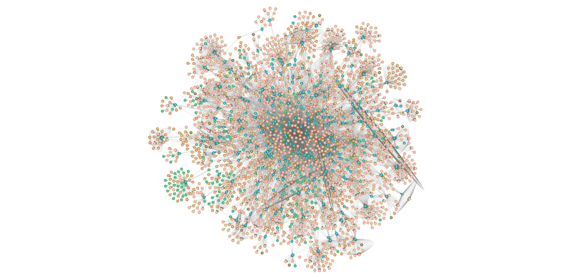
If you’re a fan of crime shows, you would have come across scenes like a detective putting together evidence, such as pictures, notes and articles, on a board and connecting them with thumb tacks and yarn. When you look at the board, it’s easy to see the relationships between the different pieces of evidence. That’s what graphs do, especially in fraud detection.
In the same way, while graph data is the raw material of an investigation, some of the most interesting relationships are often inferred rather than modelled directly in the data. Visualising these relationships can give a unique “big picture” of the data that is difficult or impossible to obtain with traditional relational tables and business intelligence tools.
On the other hand, graph visualisation enhances the quick identification of relationships and significant structures because it is an intuitive way to help detect patterns. Plus, the human brain processes visual information much faster; that’s where our Graph Visualisation platform comes in.
What is the Graph Visualisation platform?
Graph Visualisation platform is a full-featured investigation platform that can reveal hidden connections and context in data by transforming raw records into highly visual and interactive maps. From there, investigators can grab any data point and quickly see relationships, patterns, and anomalies, and if necessary, drill down to investigate further.
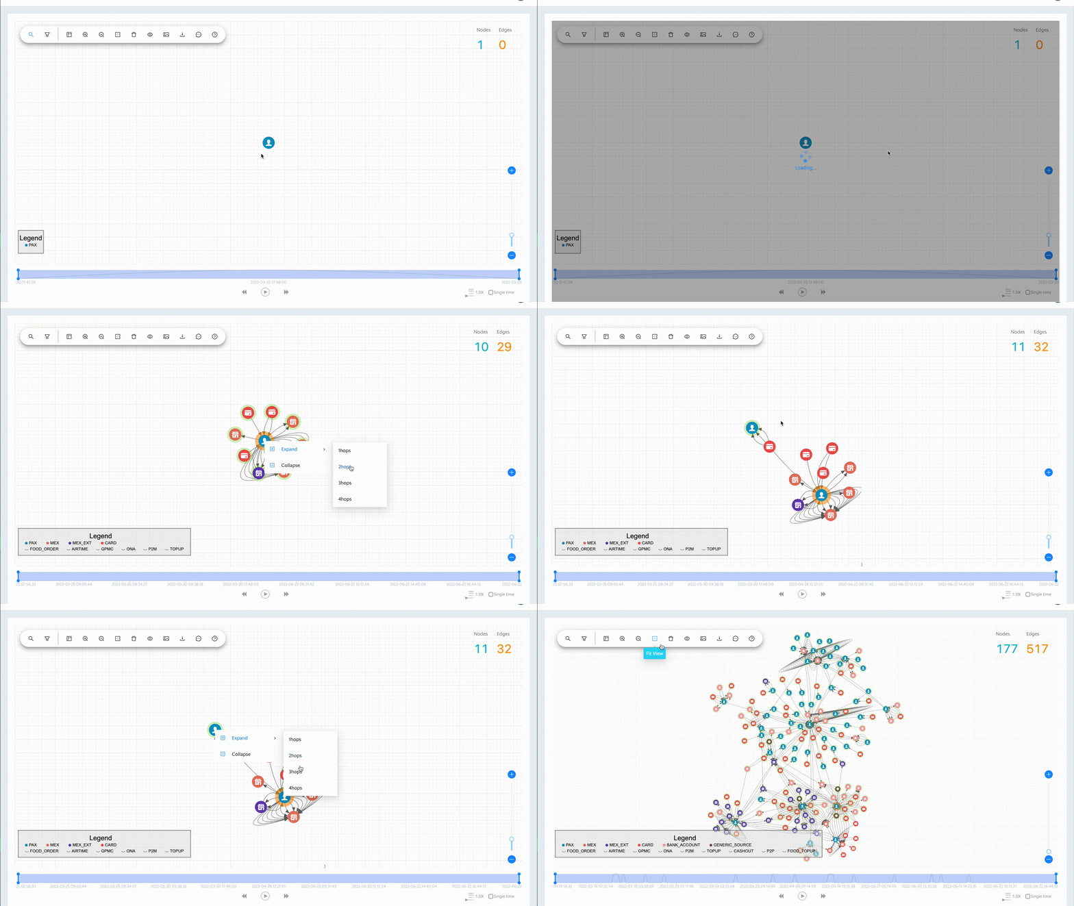
This is all done without writing a manual query, switching between anti-fraud systems, or having to think about data science! These are some of the interactions on the platform that easily make anomalies or relevant patterns stand out.
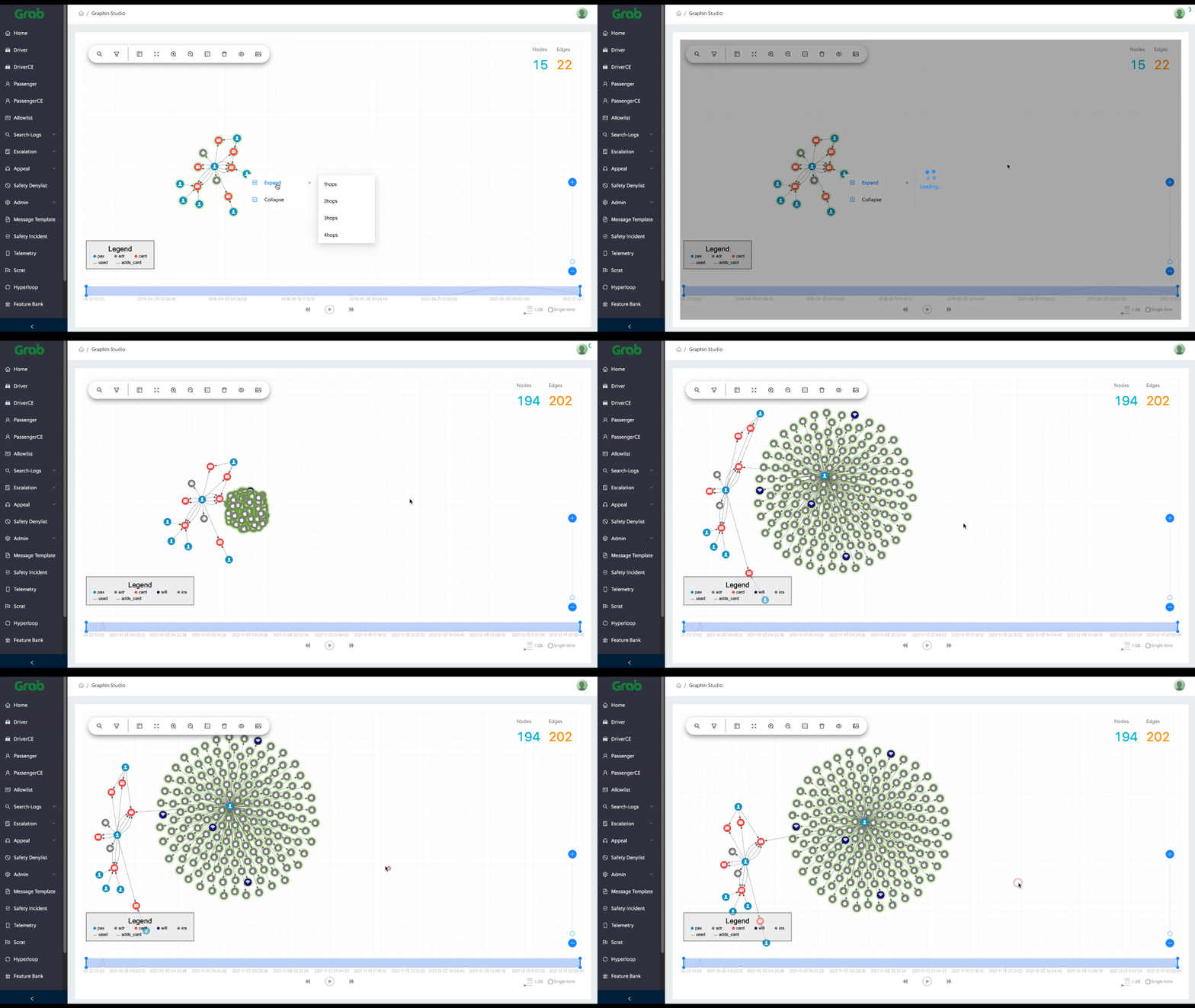
Expanding the data
To date, we have over three billion nodes and edges in our storage system. It is not possible (nor necessary) to show all of the data at once. The platform allows the user to grab any data point and easily expand to view the relationships.
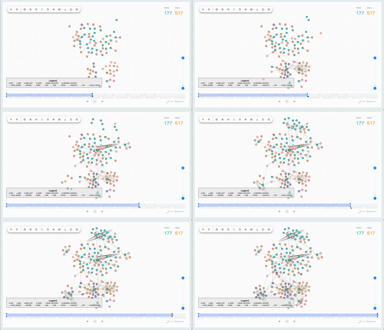
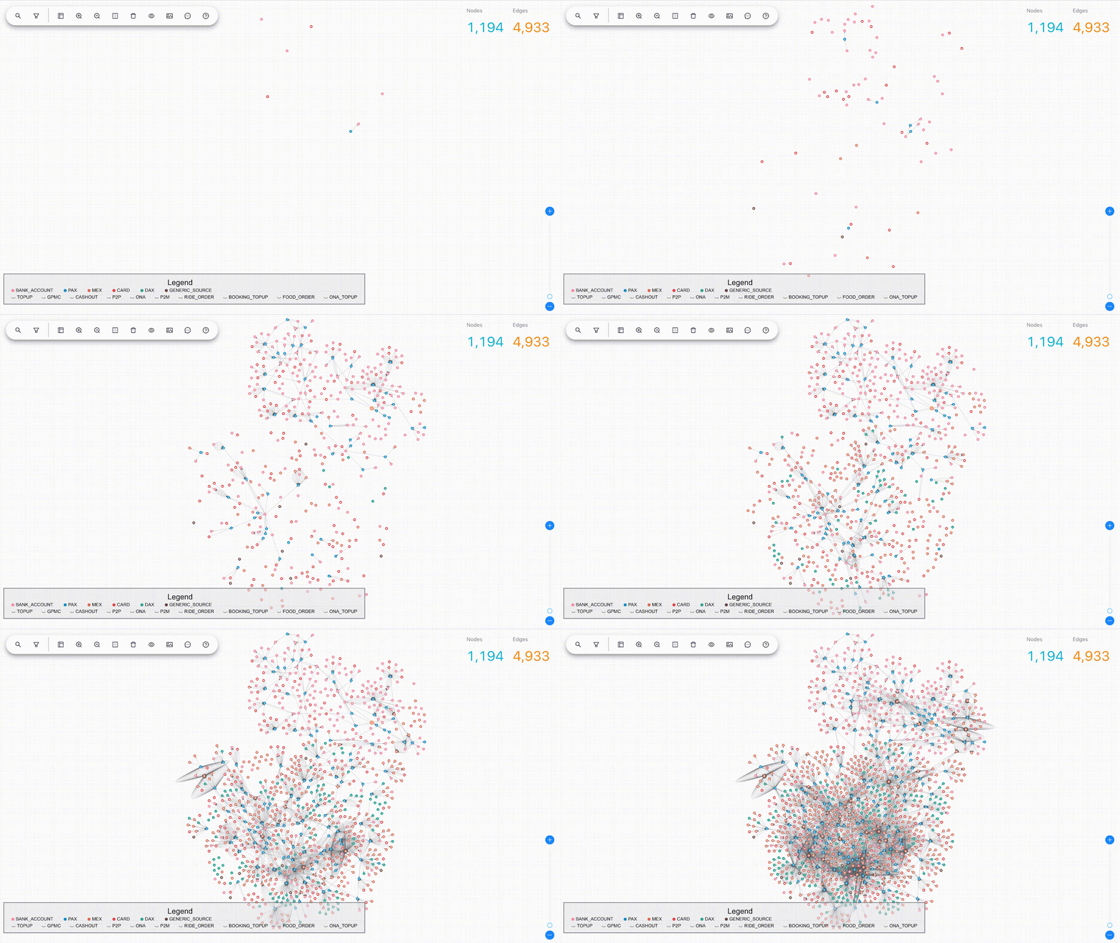
Timeline tracking and history replay
The Graph Visualisation platform’s interactive time filter lets you see temporal relationships within your data and clearly reveals the chronological progression of events. You can start with a specific time of interest, track everything that happens after, then quickly focus on the time and relationships that matter most.
10X investigations
Here are a few examples of how the Graph Visualisation platform facilitates fraud investigations.
Appeal confirmation
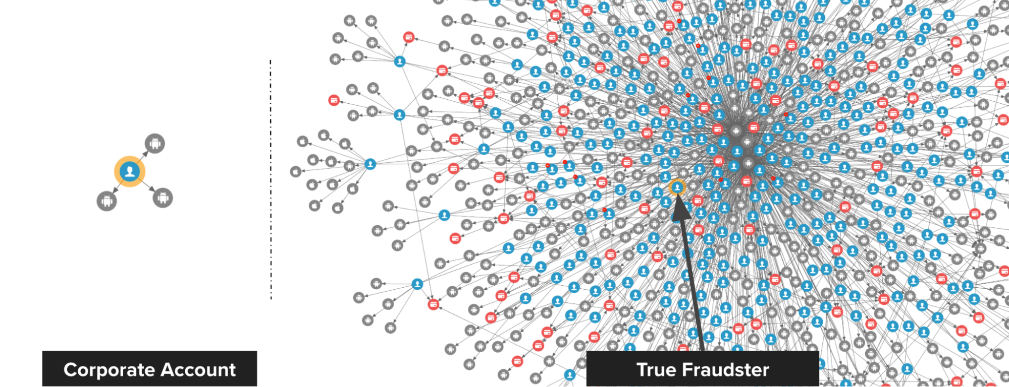
The following image shows the difference between a true fraudster and a falsely identified one. On the left, we have a Grab rental corporate account that was falsely detected by a fraud rule. Upon review, we discovered that there is no suspicious connection to this account, thus the account got unblocked.
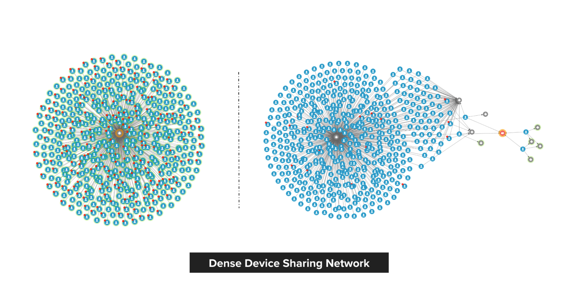
On the right, we have a passenger that was blocked by the system and they appealed. Investigations showed that the passenger is, in fact, part of an extremely dense device-sharing network, so we maintained our decision to block.
Modus operandi discovery
Passenger sharing device
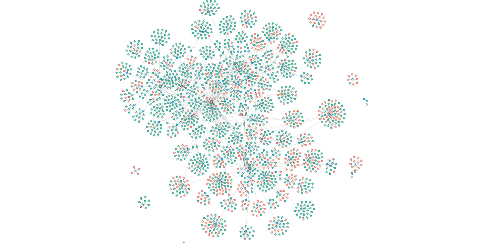
Fraudsters tend to share physical resources to maximise their revenue. With our Graph Visualisation platform, you can see exactly how this pattern looks like. The image below shows a device that is shared by a lot of fraudsters.
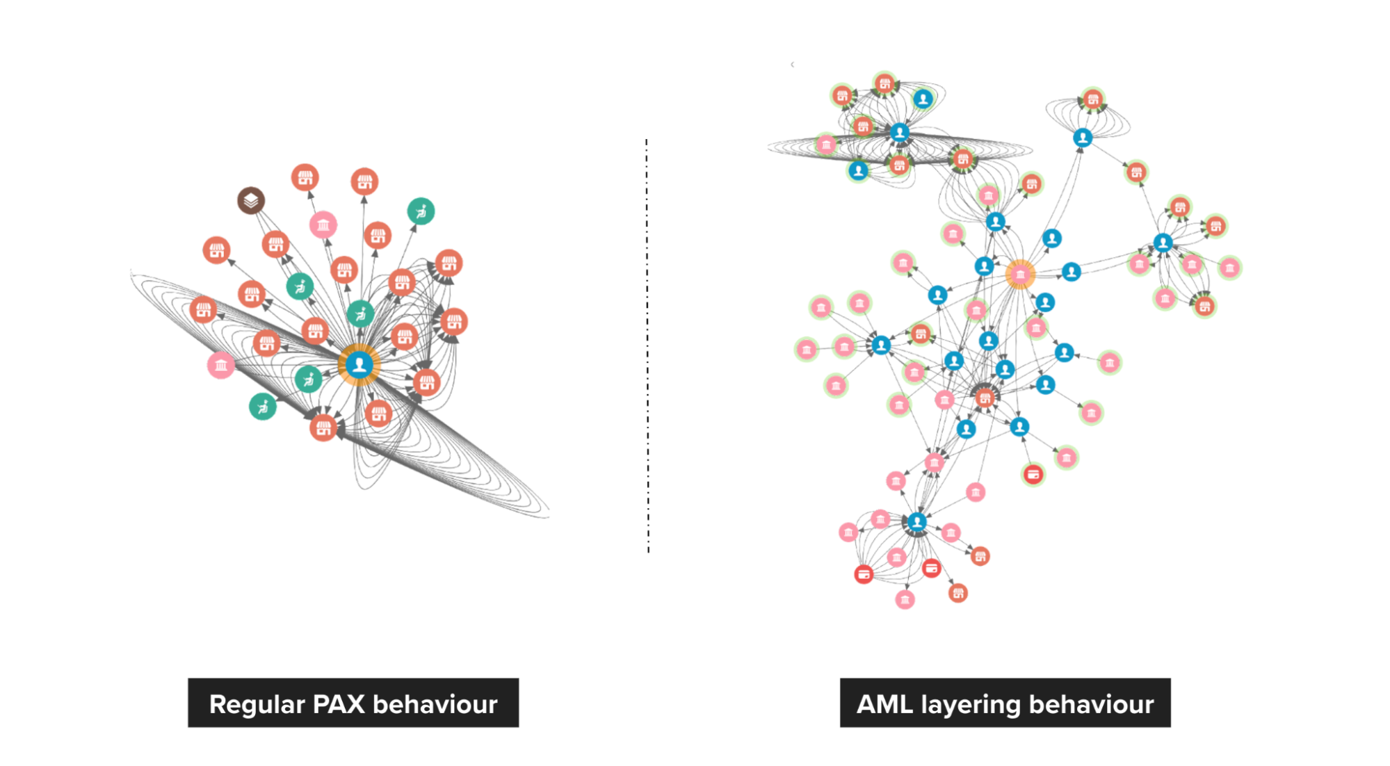
Anti-money laundering (AML)
On the left, we see a pattern of healthy spending on Grab. However, on the right, we can see that passengers are highly connected, and it has frequent large amount transfers to other payment providers.
Closing thoughts
Graph Visualisation is an intuitive way to investigate suspicious connections and potential patterns of crime. Investigators can directly interact with any data point to get the details they need and literally view the relationships in the data to make fast, accurate, and defensible decisions.
While fraud detection is a good use case for Graph Visualisation, it’s not the only possibility. Graph Visualisation can help make anything more efficient and intelligent, especially if you have highly connected data.
In the next part of this blog series, we will talk about the Graph service platform and the importance of building graph services with graph databases. Check out the other articles in this series:
Grab is the leading superapp platform in Southeast Asia, providing everyday services that matter to consumers. More than just a ride-hailing and food delivery app, Grab offers a wide range of on-demand services in the region, including mobility, food, package and grocery delivery services, mobile payments, and financial services across 428 cities in eight countries.
Powered by technology and driven by heart, our mission is to drive Southeast Asia forward by creating economic empowerment for everyone. If this mission speaks to you, join our team today!
Facial recognition technology is one of the many modern technologies that previously only appeared in science fiction movies. The roots of this technology can be traced back to the 1960s and have since grown dramatically due to the rise of deep learning techniques and accelerated digital transformation in recent years.
In this blog post, we will talk about the various applications of facial recognition technology in Grab, as well as provide details of the technical components that build up this technology.
Application of facial recognition technology
At Grab, we believe in prevention, protection, and action to create a safer every day for our consumers, partners, and the community as a whole. All selfies collected by Grab are handled according to Grab’s Privacy Policy and securely protected under privacy legislation in the countries in which we operate. We will elaborate in detail in a section further below.
One key incident prevention method is to verify the identity of both our consumers and partners:
From the perspective of protecting the safety of passengers, having a reliable driver authentication process can avoid unauthorized people from delivering a ride. This ensures that trips on Grab are only completed by registered licensed driver-partners that have passed our comprehensive background checks.
From the perspective of protecting the safety of driver-partners, verifying the identity of new passengers using facial recognition technology helps to deter crimes targeting our driver-partners and make incident investigations easier.
Safety incidents that arise from lack of identity verification
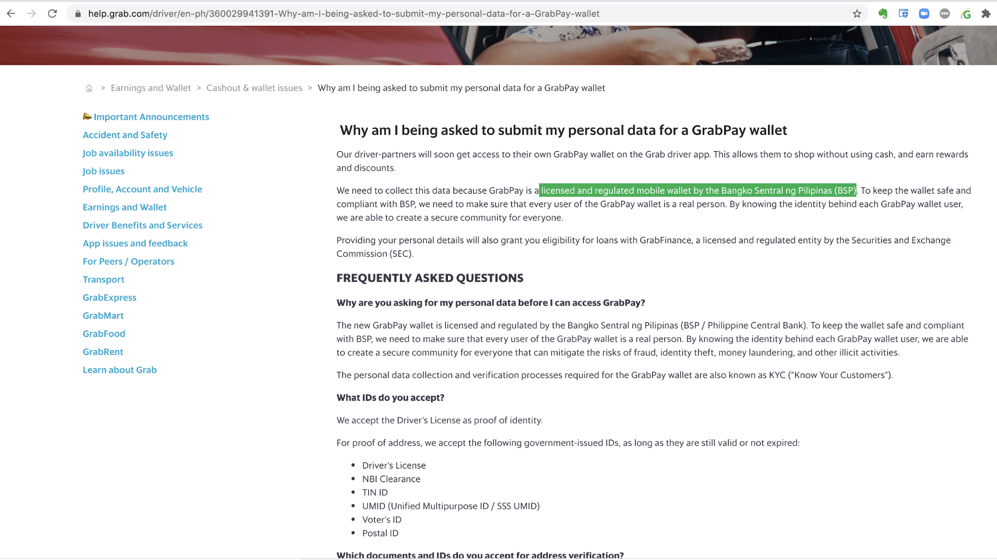
Facial recognition technology is also leveraged to improve Grab digital financial services, particularly in facilitating the “electronic Know Your Customer” (e-KYC) process. KYC is a standard regulatory requirement in the financial services industry to verify the identity of customers, which commonly serves to deter financial crime, such as money laundering.
Traditionally, customers are required to visit a physical counter to verify their government-issued ID as proof of identity. Today, with the widespread use of mobile devices, coupled with the maturity of facial recognition technologies, the process has become much more seamless and can be done entirely digitally.
Figure 1: GrabPay wallet e-KYC regulatory requirements in the Philippines
Overview of facial recognition technology
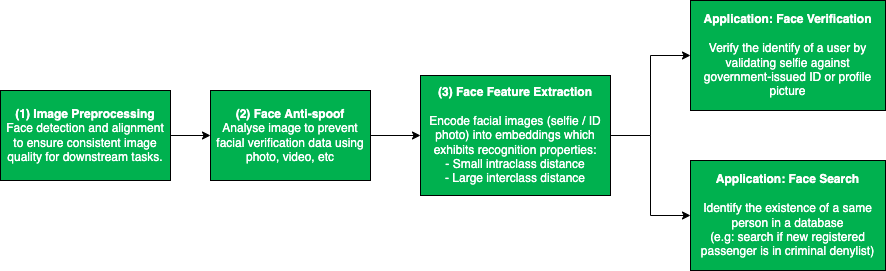
Figure 2: Face recognition flow
The typical facial recognition pipeline involves multiple stages, which starts with image preprocessing, face anti-spoof, followed by feature extraction, and finally the downstream applications – face verification or face search.
The most common image preprocessing techniques for face recognition tasks are face detection and face alignment. The face detection algorithm locates the face region in an image, and is usually followed by face alignment, which identifies the key facial landmarks (e.g. left eye, right eye, nose, etc.) and transforms them into a standardised coordinate space. Both of these preprocessing steps aim to ensure a consistent quality of input data for downstream applications.
Face anti-spoof refers to the process of ensuring that the user-submitted facial image is legitimate. This is to prevent fraudulent users from stealing identities (impersonating someone else by using a printed photo or replaying videos from mobile screens) or hiding identities (e.g. wearing a mask). The main approach here is to extract low-level spoofing cues, such as the moiré pattern, using various machine learning techniques to determine whether the image is spoofed.
After passing the anti-spoof checks, the user-submitted images are sent for face feature extraction, where important features that can be used to distinguish one person from another are extracted. Ideally, we want the feature extraction model to produce embeddings (i.e. high-dimensional vectors) with small intra-class distance (i.e. faces of the same person) and large inter-class distance (i.e. faces of different people), so that the aforementioned downstream applications (i.e. face verification and face search) become a straightforward task – thresholding the distance between embeddings.
Face verification is one of the key applications of facial recognition and it answers the question, “Is this the same person?”. As previously alluded to, this can be achieved by comparing the distance between embeddings generated from a template image (e.g. government-issued ID or profile picture) and a query image submitted by the user. A short distance indicates that both images belong to the same person, whereas a large distance indicates that these images are taken from different people.
Face search, on the other hand, tackles the question, “Who is this person?”, which can be framed as a vector/embedding similarity search problem. Image embeddings belonging to the same person would be highly similar, thus ranked higher, in search results. This is particularly useful for deterring criminals from re-onboarding to our platform by blocking new selfies that match a criminal profile in our criminal denylist database.
Face anti-spoof
For face anti-spoof, the most common methods used to attack the facial recognition system are screen replay and printed paper. To distinguish these spoof attacks from genuine faces, we need to solve two main challenges.
The first challenge is to obtain enough data of spoof attacks to enable the training of models. The second challenge is to carefully train the model to focus on the subtle differences between spoofed and genuine cases instead of overfitting to other background information.
Figure 3: Original face (left), screen replay attack (middle), synthetic data with a moiré pattern (right)
Collecting large volumes of spoof data is naturally hard since spoof cases in product flows are very rare. To overcome this problem, one option is to synthesise large volumes of spoof data instead of collecting the real spoof data. More specifically, we synthesise moiré patterns on genuine face images that we have, and use the synthetic data as the screen replay attack data. This allows our model to use small amounts of real spoof data and sufficiently identify spoofing, while collecting more data to train the model.
Figure 4: Data preparation with patch data
On the other hand, a spoofed face image contains lots of information with subtle spoof cues such as moiré patterns that cannot be detected by the naked eye. As such, it’s important to train the model to identify spoof cues instead of focusing on the possible domain bias between the spoof data and genuine data. To achieve this, we need to change the way we prepare the training data.
Instead of using the entire selfie image as the model input, we firstly detect and crop the face area, then evenly split the cropped face area into several patches. These patches are used as input to train the model. During inference, images are also split into patches the same way and the final result will be the average of outputs from all patches. After this data preprocessing, the patches will contain less global semantic information and more local structure features, making it easier for the model to learn and distinguish spoofed and genuine images.
Face verification
“Data is food for AI.” – Andrew Ng, founder of Google Brain
The key success factors of artificial intelligence (AI) models are undoubtedly driven by the volume and quality of data we hold. At Grab, we have one of the largest and most comprehensive face datasets, covering a wide range of demographic groups in Southeast Asia. This gives us a strong advantage to build a highly robust and unbiased facial recognition model that serves the region better.
As mentioned earlier, all selfies collected by Grab are securely protected under privacy legislation in the countries in which we operate. We take reasonable legal, organisational and technical measures to ensure that your Personal Data is protected, which includes measures to prevent Personal Data from getting lost, or used or accessed in an unauthorised way. We limit access to these Personal Data to our employees on a need to know basis. Those processing any Personal Data will only do so in an authorised manner and are required to treat the information with confidentiality.
Also, selfie data will not be shared with any other parties, including our driver, delivery partners or any other third parties without proper authorisation from the account holder. They are strictly used to improve and enhance our products and services, and not used as a means to collect personal identifiable data. Any disclosure of personal data will be handled in accordance with Grab Privacy Policy.
Other than data, model architecture also plays an important role, especially when handling less common face verification scenarios, such as ”selfie to ID photo” and “selfie to masked selfie” verifications.
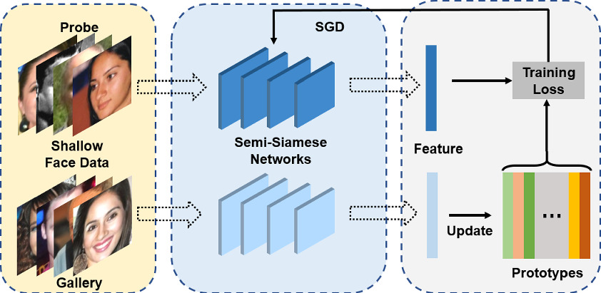
The main challenge of “selfie to ID photo” verification is the shallow nature of the dataset, i.e. a large number of unique identities, but a low number of image samples per identity. This type of dataset lacks representation in intra-class diversity, which would commonly lead to model collapse during model training. Besides, “selfie to ID photo” verification also poses numerous challenges that are different from general facial recognition, such as aging (old ID photo), attrited ID card (normal wear and tear), and domain difference between printed ID photo and real-life selfie photo.
To address these issues, we leveraged a novel training method named semi-Siamese training (SST) 2, which is proposed by Du et al. (2020). The key idea is to enlarge intra-class diversity by ensuring that the backbone Siamese networks have similar parameters, but are not entirely identical, hence the name “semi-Siamese”.
Just like typical Siamese network architecture, feature vectors generated by the subnetworks are compared to compute the loss functions, such as Arc-softmax, Triplet loss, and Large margin cosine loss, all of which aim to reduce intra-class distance while increasing the inter-class distances. With the usage of the semi-Siamese backbone network, intra-class diversity is further promoted as it is guaranteed by the difference between the subnetworks, making the training convergence more stable.
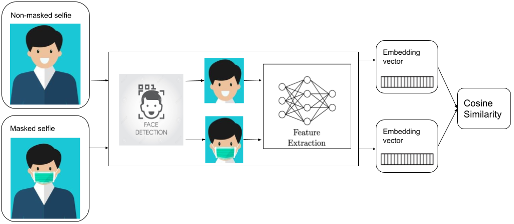
Figure 6: Masked face verification
Another type of face verification problem we need to solve these days is the “selfie to masked selfie” verification. To pass this type of face verification, users are required to take off their masks as previous face verification models are unable to verify people with masks on. However, removing face masks to do face verification is inconvenient and risky in a crowded environment, which is a pain for many of our driver-partners who need to do verification from time to time.
To help ease this issue, we developed a face verification model that can verify people even while they are wearing masks. This is done by adding masked selfies into the training data and training the model with both masked and unmasked selfies. This not only enables the model to perform verification for people with masks on, but also helps to increase the accuracy of verifying those without masks. On top of that, masked selfies act as data augmentation and help to train the model with stronger ability of extracting features from the face.
Face search
As previously mentioned, once embeddings are produced by the facial recognition models, face search is fundamentally no different from face verification. Both processes use the distance between embeddings to decide whether the faces belong to the same person. The only difference here is that face search is more computationally expensive, since face verification is a 1-to-1 comparison, whereas face search is a 1-to-N comparison (N=size of the database).
In practice, there are many ways to significantly reduce the complexity of the search algorithm from O(N), such as using Inverted File Index (IVF) and Hierarchical Navigable Small World (HNSW) graphs. Besides, there are also various methods to increase the query speed, such as accelerating the distance computation using GPU, or approximating the distances using compressed vectors. This problem is also commonly known as Approximate Nearest Neighbor (ANN). Some of the great open-sourced vector similarity search libraries that can help to solve this problem are ScaNN3 (by Google), FAISS4(by Facebook), and Annoy (by Spotify).
What’s next?
In summary, facial recognition technology is an effective crime prevention and reduction tool to strengthen the safety of our platform and users. While the enforcement of selfie collection by itself is already a strong deterrent against fraudsters misusing our platform, leveraging facial recognition technology raises the bar by helping us to quickly and accurately identify these offenders.
As technologies advance, face spoofing patterns also evolve. We need to continuously monitor spoofing trends and actively improve our face anti-spoof algorithms to proactively ensure our users’ safety.
With the rapid growth of facial recognition technology, there is also a growing concern regarding data privacy issues. At Grab, consumer privacy and safety remain our top priorities and we continuously look for ways to improve our existing safeguards.
In May 2022, Grab was recognised by the Infocomm Media Development Authority in Singapore for its stringent data protection policies and processes through the award of Data Protection Trustmark (DPTM) certification. This recognition reinforces our belief that we can continue to draw the benefits from facial recognition technology, while avoiding any misuse of it. As the saying goes, “Technology is not inherently good or evil. It’s all about how people choose to use it”.
Join us
Grab is the leading superapp platform in Southeast Asia, providing everyday services that matter to consumers. More than just a ride-hailing and food delivery app, Grab offers a wide range of on-demand services in the region, including mobility, food, package and grocery delivery services, mobile payments, and financial services across 428 cities in eight countries.
Powered by technology and driven by heart, our mission is to drive Southeast Asia forward by creating economic empowerment for everyone. If this mission speaks to you, join our team today!
References
Niu, D., Guo R., and Wang, Y. (2021). Moiré Attack (MA): A New Potential Risk of Screen Photos. Advances in Neural Information Processing Systems. https://papers.nips.cc/paper/2021/hash/db9eeb7e678863649bce209842e0d164-Abstract.html ↩
Du, H., Shi, H., Liu, Y., Wang, J., Lei, Z., Zeng, D., & Mei, T. (2020). Semi-Siamese Training for Shallow Face Learning. European Conference on Computer Vision, 36–53. Springer. ↩
Guo, R., Sun, P., Lindgren, E., Geng, Q., Simcha, D., Chern, F., & Kumar, S. (2020). Accelerating Large-Scale Inference with Anisotropic Vector Quantization. International Conference on Machine Learning. https://arxiv.org/abs/1908.10396 ↩
Johnson, J., Douze, M., & Jégou, H. (2019). Billion-scale similarity search with GPUs. IEEE Transactions on Big Data, 7(3), 535–547. ↩
In an introductory article, we talked about the importance of Graph Networks in fraud detection. In this article, we will be adding some further context on graphs, graph technology and some common use cases.
Connectivity is the most prominent feature of today’s networks and systems. From molecular interactions, social networks and communication systems to power grids, shopping experiences or even supply chains, networks relating to real-world systems are not random. This means that these connections are not static and can be displayed differently at different times. Simple statistical analysis is insufficient to effectively characterise, let alone forecast, networked system behaviour.
As the world becomes more interconnected and systems become more complex, it is more important to employ technologies that are built to take advantage of relationships and their dynamic properties. There is no doubt that graphs have sparked a lot of attention because they are seen as a means to get insights from related data. Graph theory-based approaches show the concepts underlying the behaviour of massively complex systems and networks.
What are graphs?
Graphs are mathematical models frequently used in network science, which is a set of technological tools that may be applied to almost any subject. To put it simply, graphs are mathematical representations of complex systems.
Origin of graphs
The first graph was produced in 1736 in the city of Königsberg, now known as Kaliningrad, Russia. In this city, there were two islands with two mainland sections that were connected by seven different bridges.
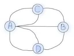
Famed mathematician Euler wanted to plot a journey through the entire city by crossing each bridge only once. Euler proceeded to abstract the four regions of the city and the seven bridges into edges but he demonstrated that the problem was unsolvable. A simplified abstract graph is shown in Fig 1.
Fig 1 Abstraction graph
The graph’s four dots represent Königsberg’s four zones, while the lines represent the seven bridges that connect them. Zones connected by an even number of bridges is clearly navigable because several paths to enter and exit are available. Zones connected by an odd number of bridges can only be used as starting or terminating locations because the same route can only be taken once.
The number of edges associated with a node is known as the node degree. If two nodes have odd degrees and the rest have even degrees, the Königsberg problem could be solved. For example, exactly two regions must have an even number of bridges while the rest have an odd number of bridges. However, as illustrated in Fig 1, no Königsberg location has an even number of bridges, rendering this problem unsolvable.
Definition of graphs
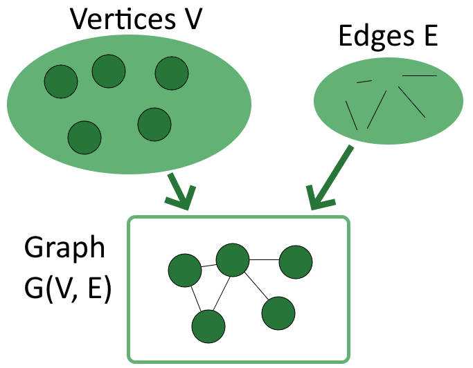
A graph is a structure that consists of vertices and edges. Vertices, or nodes, are the objects in a problem, while edges are the links that connect vertices in a graph.
Vertices are the fundamental elements that a graph requires to function; there should be at least one in a graph. Vertices are mathematical abstractions that refer to objects that are linked by a condition.
On the other hand, edges are optional as graphs can still be defined without any edges. An edge is a link or connection between any two vertices in a graph, including a connection between a vertex and itself. The idea is that if two vertices are present, there is a relationship between them.
We usually indicate V={v1, v2, …, vn} as the set of vertices, and E = {e1, e2, …, em} as the set of edges. From there, we can define a graph G as a structure G(V, E) which models the relationship between the two sets:
Fig 2 Graph structure
It is worth noting that the order of the two sets within parentheses matters, because we usually express the vertices first, followed by the edges. A graph H(X, Y) is therefore a structure that models the relationship between the set of vertices X and the set of edges Y, not the other way around.
Graph data model
Now that we have covered graphs and their typical components, let us move on to graph data models, which help to translate a conceptual view of your data to a logical model. Two common graph data formats are Resource Description Framework (RDF) and Labelled Property Graph (LPG).
Resource Description Framework (RDF)
RDF is typically used for metadata and facilitates standardised exchange of data based on their relationships. RDFs typically consist of a triple: a subject, a predicate, and an object. A collection of such triples is an RDF graph. This can be depicted as a node and a directed edge diagram, with each triple representing a node-edge-node graph, as shown in Fig 3.
Literals – data type value, i.e. text, integer, etc.
Blank nodes – have no identification; similar to anonymous or existential variables.
Let us use an example to illustrate this. We have a person with the name Art and we want to plot all his relationships. In this case, the IRI is http://example.org/art and this can be shortened by defining a prefix like ex.
In this example, the IRI http://xmlns.com/foaf/0.1/knows defines the relationship knows. We define foaf as the prefix for http://xmlns.com/foaf/0.1/. The following code snippet shows how a graph like this will look.
In the last two lines, you can see how a literal and blank node would be depicted in an RDF graph. The variable foaf:age is a literal node with the integer value of 23, while foaf:based_near is an anonymous spatial entity with a node identifier of underscore. Outside the context of this graph, o1 is a data identifier with no meaning.
Multiple IRIs, intended for use in RDF graphs, are typically stored in an RDF vocabulary. These IRIs often begin with a common substring known as a namespace IRI. In some cases, namespace IRIs are also associated with a short name known as a namespace prefix. In the example above, http://xmlns.com/foaf/0.1/ is the namespace IRI and foaf and ex are namespace prefixes.
Note: RDF graphs are considered atemporal as they provide a static snapshot of data. They can use appropriate language extensions to communicate information about events or other dynamic properties of entities.
An RDF dataset is a set of RDF graphs that includes one or more named graphs as well as exactly one default graph. A default graph is one that can be empty, and has no associated IRI or name, while each named graph has an IRI or a blank node corresponding to the RDF graph and its name. If there is no named graph specified in a query, the default graph is queried (hence its name).
Labelled Property Graph (LPG)
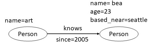
A labelled property graph is made up of nodes, links, and properties. Each node is given a label and a set of characteristics in the form of arbitrary key-value pairs. The keys are strings, and the values can be any data type. A relationship is then defined by adding a directed edge that is labelled and connects two nodes with a set of properties.
In Fig 4, we have an LPG that shows two nodes: art and bea. The bea node has two characteristics, age and proximity, that are connected by a known edge. This edge has the attribute since because it commemorates the year that art and bea first met.
Fig 4 Labelled Property Graph: Example 1
Nodes, edges and properties must be defined when designing an LPG data model. In this scenario, based_near might not be applicable to all vertices, but they should be defined. You might be wondering, why not represent the city Seattle as a node and add an edge marked as based_near that connects a person and the city?
In general, if there is a value linked to a large number of other nodes in the network and it requires additional properties to correlate with other nodes, it should be represented as a node. In this scenario, the architecture defined in Fig 5 is more appropriate for traversing based_near connections. It also gives us the ability to link any new attributes to the based_near relationship.
Fig 5 Labelled Property Graph: Example 2
Now that we have the context of graphs, let us talk about graph databases, how they help with large data queries and the part they play in Graph Technology.
Graph database
A graph database is a type of NoSQL database that stores data using network topology. The idea is derived from LPG, which represents data sets with vertices, edges, and attributes.
Vertices are instances or entities of data that represent any object to be tracked, such as people, accounts, locations, etc.
Edges are the critical concepts in graph databases which represent relationships between vertices. The connections have a direction that can be unidirectional (one-way) or bidirectional (two-way).
Properties represent descriptive information associated with vertices. In some cases, edges have properties as well.
Graph databases provide a more conceptual view of data that is closer to reality. Modelling complex linkages becomes simpler because interconnections between data points are given the same weight as the data itself.
Graph database vs. relational database
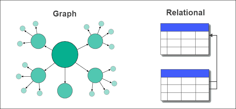
Relational databases are currently the industry norm and take a structured approach to data, usually in the form of tables. On the other hand, graph databases are agile and focus on immediate relationship understanding. Neither type is designed to replace the other, so it is important to know what each database type has to offer.
Fig 6 Graph database vs relational database
There is a domain for both graph and relational databases. Graph databases outperform typical relational databases, especially in use cases involving complicated relationships, as they take a more naturalistic and flowing approach to data.
The key distinctions between graph and relational databases are summarised in the following table:
Type
Graph
Relational
Format
Nodes and edges with properties
Tables with rows and columns
Relationships
Represented with edges between nodes
Created using foreign keys between tables
Flexibility
Flexible
Rigid
Complex queries
Quick and responsive
Requires complex joins
Use case
Systems with highly connected relationships
Transaction focused systems with more straightforward relationships
Table. 1 Graph vs. Relational Databases
Advantages and disadvantages
Every database type has its advantages and disadvantages; knowing the distinctions as well as potential options for specific challenges is crucial. Graph databases are a rapidly evolving technology with improved functions compared with other database types.
Advantages
Some advantages of graph databases include:
Agile and flexible structures.
Explicit relationship representation between entities.
Real-time query output – speed depends on the number of relationships.
Disadvantages
The general disadvantages of graph databases are:
No standardised query language; depends on the platform used.
Not suitable for transactional-based systems.
Small user base, making it hard to find troubleshooting support.
Graph technology
Graph technology is the next step in improving analytics delivery. Traditional analytics is insufficient to meet complicated business operations, distribution, and analytical concerns as data quantities expand.
Graph technology aids in the discovery of unknown correlations in data that would otherwise go undetected or unanalysed. When the term graph is used to describe a topic, three distinct concepts come to mind: graph theory, graph analytics, and graph data management.
Graph theory – A mathematical notion that uses stack ordering to find paths, linkages, and networks of logical or physical objects, as well as their relationships. Can be used to model molecules, telephone lines, transport routes, manufacturing processes, and many other things.
Graph analytics – The application of graph theory to uncover nodes, edges, and data linkages that may be assigned semantic attributes. Can examine potentially interesting connections in data found in traditional analysis solutions, using node and edge relationships.
Graph database – A type of storage for data generated by graph analytics. Filling a knowledge graph, which is a model in data that indicates a common usage of acquired knowledge or data sets expressing a frequently held notion, is a typical use case for graph analytics output.
While the architecture and terminology are sometimes misunderstood, graph analytics’ output can be viewed through visualisation tools, knowledge graphs, particular applications, and even some advanced dashboard capabilities of business intelligence tools. All three concepts above are frequently used to improve system efficiency and even to assist in dynamic data management. In this approach, graph theory and analysis are inextricably linked, and analysis may always rely on graph databases.
Graph-centric user stories
Fraud detection
Traditional fraud prevention methods concentrate on discrete data points such as individual accounts, devices, or IP addresses. However, today’s sophisticated fraudsters avoid detection by building fraud rings using stolen and fake identities. To detect such fraud rings, we need to look beyond individual data points to the linkages that connect them.
Graph technology greatly transcends the capabilities of a relational database, by revealing hard-to-find patterns. Enterprise businesses also employ Graph technology to supplement their existing fraud detection skills to tackle a wide range of financial crimes, including first-party bank fraud, fraud, and money laundering.
Real-time recommendations
An online business’s success depends on systems that can generate meaningful recommendations in real time. To do so, we need the capacity to correlate product, customer, inventory, supplier, logistical, and even social sentiment data in real time. Furthermore, a real-time recommendation engine must be able to record any new interests displayed during the consumer’s current visit in real time, which batch processing cannot do.
Graph databases outperform relational and other NoSQL data stores in terms of delivering real-time suggestions. Graph databases can easily integrate different types of data to get insights into consumer requirements and product trends, making them an increasingly popular alternative to traditional relational databases.
Supply chain management
With complicated scenarios like supply chains, there are many different parties involved and companies need to stay vigilant in detecting issues like fraud, contamination, high-risk areas or unknown product sources. This means that there is a need to efficiently process large amounts of data and ensure transparency throughout the supply chain.
To have a transparent supply chain, relationships between each product and party need to be mapped out, which means there will be deep linkages. Graph databases are great for these as they are designed to search and analyse data with deep links. This means they can process enormous amounts of data without performance issues.
Identity and access management
Managing multiple changing roles, groups, products and authorisations can be difficult, especially in large organisations. Graph technology integrates your data and allows quick and effective identity and access control. It also allows you to track all identity and access authorisations and inheritances with significant depth and real-time insights.
Network and IT operations
Because of the scale and complexity of network and IT infrastructure, you need a configuration management database (CMDB) that is far more capable than relational databases. Neptune is an example of a CMDB and graph database that allows you to correlate your network, data centre, and IT assets to aid troubleshooting, impact analysis, and capacity or outage planning.
A graph database allows you to integrate various monitoring tools and acquire important insights into the complicated relationships that exist between various network or data centre processes. Possible applications of graphs in network and IT operations range from dependency management to automated microservice monitoring.
Risk assessment and monitoring
Risk assessment is crucial in the fintech business. With multiple sources of credit data such as ecommerce sites, mobile wallets and loan repayment records, it can be difficult to accurately assess an individual’s credit risk. Graph Technology makes it possible to combine these data sources, quantify an individual’s fraud risk and even generate full credit reviews.
One clear example of this is IceKredit, which employs artificial intelligence (AI) and machine learning (ML) techniques to make better risk-based decisions. With Graph technology, IceKredit has also successfully detected unreported links and increased efficiency of financial crime investigations.
Social network
Whether you’re using stated social connections or inferring links based on behaviour, social graph databases like Neptune introduce possibilities for building new social networks or integrating existing social graphs into commercial applications.
Having a data model that is identical to your domain model allows you to better understand your data, communicate more effectively, and save time. By decreasing the time spent data modelling, graph databases increase the quality and speed of development for your social network application.
Artificial intelligence (AI) and machine learning (ML)
AI and ML use statistical and analytical approaches to find patterns in data and provide insights. However, there are two prevalent concerns that arise – the quality of data and effectiveness of the analytics. Some AI and ML solutions have poor accuracy because there is not enough training data or variants that have a high correlation to the outcome.
These ML data issues can be solved with graph databases as it’s possible to connect and traverse links, as well as supplement raw data. With Graph technology, ML systems can recognise each column as a “feature” and each connection as a distinct characteristic, and then be able to identify data patterns and train themselves to recognise these relationships.
Conclusion
Graphs are a great way to visually represent complex systems and can be used to easily detect patterns or relationships between entities. To help improve graphs’ ability to detect patterns early, businesses should consider using Graph technology, which is the next step in improving analytics delivery.
Graph technology typically consists of:
Graph theory – Used to find paths, linkages and networks of logical or physical objects.
Graph analytics – Application of graph theory to uncover nodes, edges, and data linkages.
Graph database – Storage for data generated by graph analytics.
Although predominantly used in fraud detection, Graph technology has many other use cases such as making real-time recommendations based on consumer behaviour, identity and access control, risk assessment and monitoring, AI and ML, and many more.
Check out our next blog article, where we will be talking about how our Graph Visualisation Platform enhances Grab’s fraud detection methods.
Grab is the leading superapp platform in Southeast Asia, providing everyday services that matter to consumers. More than just a ride-hailing and food delivery app, Grab offers a wide range of on-demand services in the region, including mobility, food, package and grocery delivery services, mobile payments, and financial services across 428 cities in eight countries.
Powered by technology and driven by heart, our mission is to drive Southeast Asia forward by creating economic empowerment for everyone. If this mission speaks to you, join our team today!
Trustworthy experiments are key to making sound decisions, so analysts and data scientists put a lot of effort into analysing them and making business impacts. An extension of Grab’s Experimentation (GrabX) platform, Automated Experiment Analysis is one of Grab’s data products that helps automate statistical analyses of experiments. It also provides automatic experimental data pipelines and customised tests for different types of experiments.
Designed to help Grab in its journey of innovation and data-driven decision making, the data product helps to:
Standardise and automate the basic experiment analysis process on Grab experiments.
Ensure post-experiment results are reproducible under a company-wide standard, and easily reviewed by each other.
Democratise the institutional knowledge of experimentation across functions.
Background
Today, the GrabX platform provides the ability to define, configure, and execute online controlled experiments (OCEs), often called A/B tests, to gather trustworthy data and make data-driven decisions about how to improve our products.
Before the automated analysis, each experiment was analysed manually on an ad-hoc basis. This manual and federated model brings in several challenges at the company level:
Inefficiency: Repetitive nature of data pipeline building and basic post-experiment analyses incur large costs and deplete the analysts’ bandwidth from running deeper analyses.
Lack of quality control: Risk of unstandardised, inaccurate or late results as the platform cannot exercise data-governance/control or extend offerings to Grab’s other entities.
Lack of scalability and availability: GrabX users have varied backgrounds and skills, making their approaches to experiments different and not easily transferable/shared. E.g. Some teams may use more advanced techniques to speed up their experiments without using too much resources but these techniques are not transferable without considerable training.
Solution
Architecture details
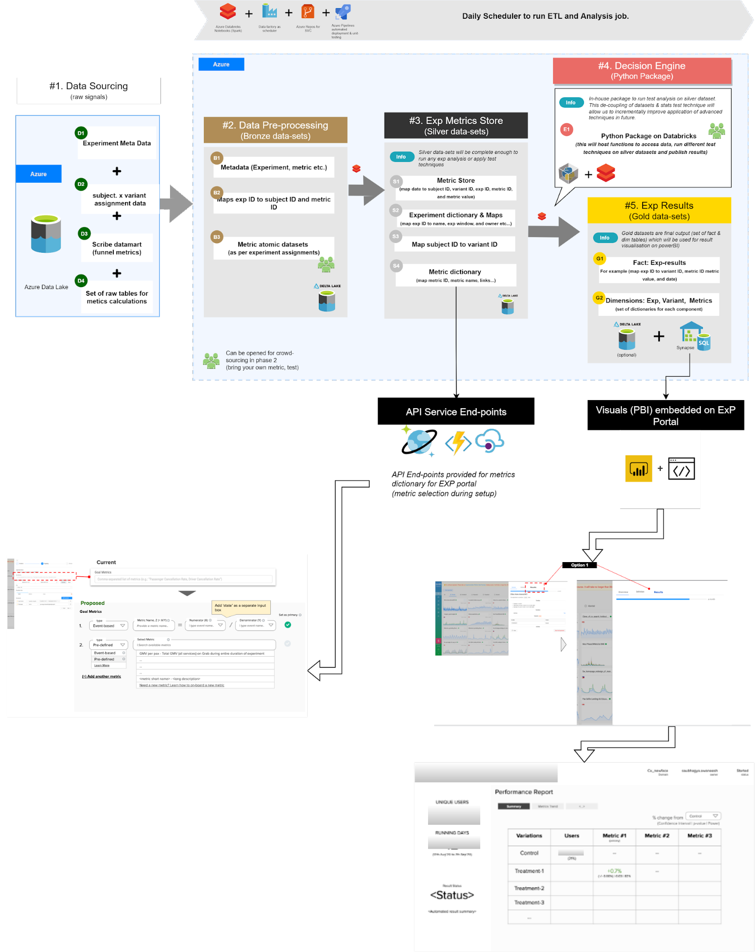
Architecture diagram
When users set up experiments on GrabX, they can configure the success metrics they are interested in. These metrics configurations are then stored in the metadata as “bronze”, “silver”, and “gold” datasets depending on the corresponding step in the automated data pipeline process.
Metrics configuration and “bronze” datasets
In this project, we have developed a metrics glossary that stores information about what the metrics are and how they are computed. The metrics glossary is stored in CosmoDB and serves as an API Endpoint for GrabX so users can pick from the list of available metrics. If a metric is not available, users can input their custom metrics definition.
This metrics selection, as an analysis configuration, is then stored as a “bronze” dataset in Azure Data Lake as metadata, together with the experiment configurations. Once the experiment starts, the data pipeline gathers all experiment subjects and their assigned experiment groups from our clickstream tracking system.
In this case, the experiment subject refers to the facets of the experiment. For example, if the experiment subject is a user, then the user will go through the same experience throughout the entire experimentation period.
Metrics computation and “silver” datasets
In this step, the metrics engine gathers all metrics data based on the metrics configuration and computes the metrics for each experiment subject. This computed data is then stored as a “silver” dataset and is the foundation dataset for all statistical analyses.
“Silver” datasets are then passed through the “Decision Engine” to get the final “gold” datasets, which contain the experiment results.
Results visualisation and ”gold” datasets
In “gold” datasets, we have the result of the experiment, along with some custom messages we want to show our users. These are saved in sets of fact and dim tables (typically used in star schemas).
For users to visualise the result on GrabX, we leverage the embedded Power BI visualisation. We build the visualisation using a “gold” dataset and embed it to each experiment page with a fixed filter. By doing so, users can experience the end-to-end flow directly from GrabX.
Implementation
The implementation consists of four key engineering components:
Analysis configuration setup
A data pipeline
Automatic analysis
Results visualisation
Analysis configuration is part of the experiment setup process where users select success metrics they are interested in. This is an essential configuration for post-experiment analysis, in addition to the usual experiment configurations (e.g. sampling strategies).
It ensures that the reported experiment results will align with the hypothesis setup, which helps avoid one of the common pitfalls in OCEs 1.
There are three types of metrics available:
Pre-defined metrics: These metrics are already defined in the Scribe datamart, e.g. Gross Merchandise Value (GMV) per pax.
Event-based metrics: Users can specify an ad-hoc metric in the form of a funnel with event names for funnel start and end.
Build your own metrics: Users have the flexibility to define a metric in the form of a SQL query.
A data pipeline here mainly consists of data sourcing and data processing. We use Azure Data Factory to schedule ETL pipelines so we can calculate the metrics and statistical analysis. ETL jobs are written in spark and run using Databricks.
Data pipelines are streamlined to the following:
Load experiments and metrics metadata, defined at the experiment creation stage.
Load experiment and clickstream events.
Load experiment assignments. An experiment assignment maps a randomisation unit ID to the corresponding experiment or variant IDs.
Merge the data mentioned above for each experiment variant, and obtain sufficient data to do a deeper results analysis.
Automatic analysis uses an internal python package “Decision Engine”, which decouples the dataset and statistical tests, so that we can incrementally improve applications of advanced techniques. It provides a comprehensive set of test results at the variant level, which include statistics, p-values, confidence intervals, and the test choices that correspond to the experiment configurations. It’s a crowdsourced project which allows all to contribute what they believe should be included in fundamental post-experiment analysis.
Results visualisation leverages PowerBI, which is embedded in the GrabX UI, so users can run the experiments and review the results on a single platform.
Impact
At the individual user level, Automated Experiment Analysis is designed to enable analysts and data scientists to associate metrics with experiments, and present the experiment results in a standardised and comprehensive manner. It speeds up the decision-making process and frees up the bandwidths of analysts and data scientists to conduct deeper analyses.
At the user community level, it improves the efficiency of running experimental analysis by capturing all experiments, their results, and the launch decision within a single platform.
Learnings/Conclusion
Automated Experiment Analysis is the first building block to boost the trustworthiness of OCEs in Grab. Not all types of experiments are fully onboard, and they might not need to be. Through this journey, we believe these key learnings would be useful for experimenters and platform teams:
To standardise and simplify several experimental analysis steps, there needs to be automation data pipelines, analytics tools, and a metrics store in the infrastructure.
The “Decision Engine” analytics tool should be decoupled from the other engineering components, so that it can be incrementally improved in future.
To democratise knowledge and ensure service coverage, many components need to have a crowdsourcing feature, e.g. the metrics store has a BYOM function, and “Decision Engine” is an open-sourced internal python package.
Tracking implementation is important. To standardise data pipelines and achieve scalability, we need to standardise the way we implement tracking.
What’s next?
A centralised metric store – We built a metric calculation dictionary, which currently contains around 30-40 basic business metrics, but its functionality is limited to GrabX Experimentation use case.
If the metric store is expected to serve more general uses, it needs to be further enriched by allowing some “smarts”, e.g. fabric-agnostic metrics computations 2, other types of data slicing, and some considerations with real-time metrics or signals.
An end-to-end experiment guide rail – Currently, we provide automatic data analysis after an experiment is done, but no guardrail features at multiple experiment stages, e.g. sampling strategy choices, sample size recommendation from the planning stage, and data quality check during/after the experiment windows. Without the end-to-end guardrails, running experiments will be very prone to pitfalls. We therefore plan to add some degree of automation to ensure experiments adhere to the standards used by the post-experimental analysis.
A more comprehensive analysis toolbox – The current state of the project mainly focuses on infrastructure development, so it starts with basic frequentist’s A/B testing approaches. In future versions, it can be extended to include sequential testing, CUPED 3, attribution analysis, Causal Forest, heterogeneous treatment effects, etc.
Join us
Grab is the leading superapp platform in Southeast Asia, providing everyday services that matter to consumers. More than just a ride-hailing and food delivery app, Grab offers a wide range of on-demand services in the region, including mobility, food, package and grocery delivery services, mobile payments, and financial services across 428 cities in eight countries.
Powered by technology and driven by heart, our mission is to drive Southeast Asia forward by creating economic empowerment for everyone. If this mission speaks to you, join our team today!
References
Dmitriev, P., Gupta, S., Kim, D. W., & Vaz, G. (2017, August). A dirty dozen: twelve common metric interpretation pitfalls in online controlled experiments. In Proceedings of the 23rd ACM SIGKDD international conference on knowledge discovery and data mining (pp. 1427-1436). ↩
Deng, A., Xu, Y., Kohavi, R., & Walker, T. (2013, February). Improving the sensitivity of online controlled experiments by utilising pre-experiment data. In Proceedings of the sixth ACM international conference on Web search and data mining (pp. 123-132). ↩
Prior to 2021, Grab’s search architecture was designed to only support textual matching, which takes in a user query and looks for exact matches within the ecosystem through an inverted index. This legacy system meant that only textual matching results could be fetched.
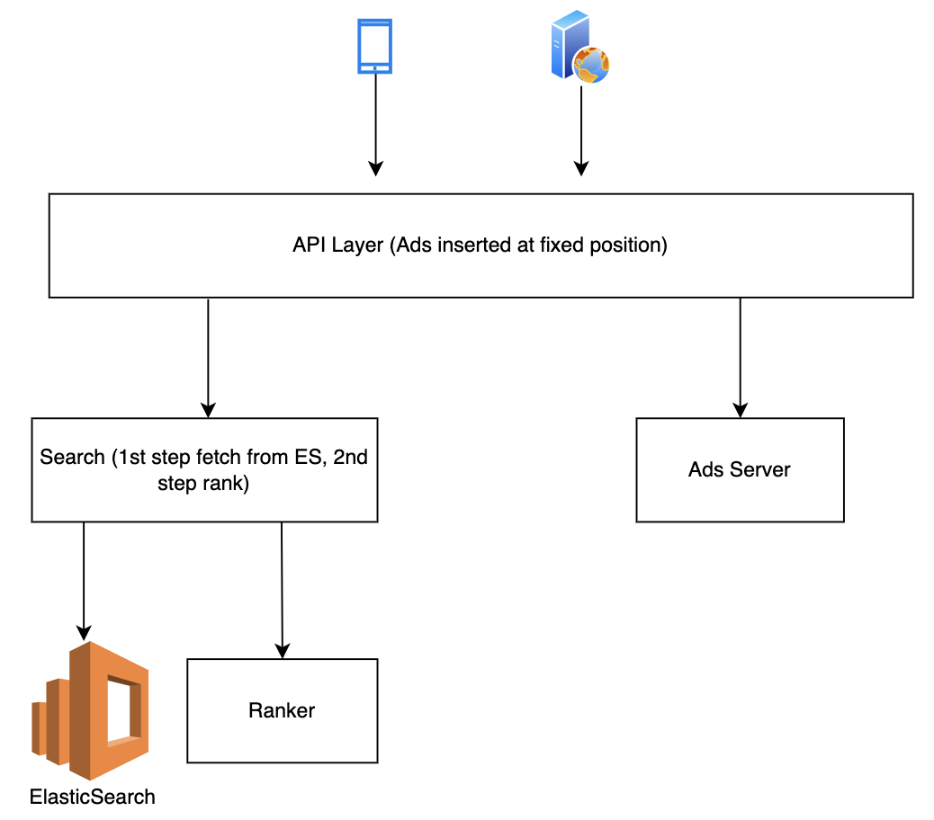
In the second half of 2021, the Deliveries search team worked on improving this architecture to make it smarter, more scalable and also unlock future growth for different search use cases at Grab. The figure below shows a simplified overview of the legacy architecture.
Legacy architecture
Problem statement
With the legacy system, we noticed several problems.
Search results were textually matched without considering intention and context
If a user types in a query “Roti Prata” (flatbread), he is likely looking for Roti Prata dishes and those matches with the dish name should be prioritised compared with matches with the merchant-partner’s name or matches with other entities.
In the legacy system, all entities whose names partially matched “Roti Prata” were displayed and ranked according to hard coded weights, and matches with merchant-partner names were always prioritised, even if the user intention was clearly to search for the “Roti Prata” dish itself.
This problem was more common in Mart, as users often intended to search for items instead of shops. Besides the lack of intention recognition, the search system was also unable to take context into consideration; users searching the same keyword query at different times and locations could have different objectives. E.g. if users search for “Bread” in the day, they may be likely to look for cafes while searches at night could be for breakfast the next day.
Search results from multiple business verticals were not blended effectively
In Grab’s context, results from multiple verticals were often merged. For example, in Mart searches, Ads and Mart organic search results were displayed together; in Food searches, Ads, Food and Mart organic results were blended together.
In the legacy architecture, multiple business verticals were merged on the Deliveries API layer, which resulted in the leak of abstraction and loss of useful data as data from the search recall stage was also not taken into account during the merge stage.
Inability to quickly scale to new search use cases and difficulty in reusing existing components
The legacy code base was not written in a structured way that could scale to new use cases easily. If new search use cases cannot be built on top of an existing system, it can be rather tedious to keep rebuilding the function every time there is a new search use case.
Solution
In this section, solutions from both architecture and implementation perspectives are presented to address the above problem statements.
Architecture
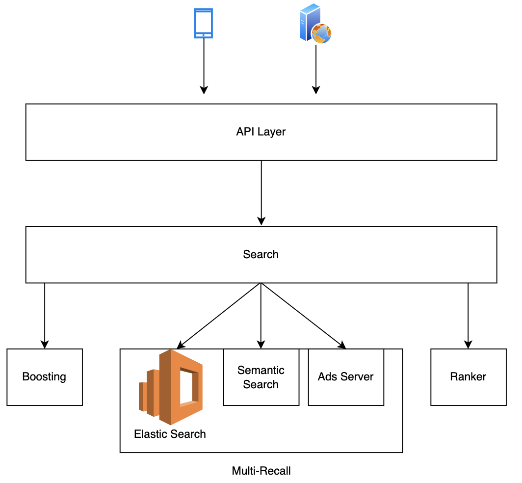
In the new architecture, the flow is extended from lexical recall only to multi-layer including boosting, multi-recall, and ranking. The addition of boosting enables capabilities like intent recognition and query expansion, while the change from single lexical recall to multi-recall opens up the potential for other recall methods, e.g. embedding based and graph based.
These help address the first problem statement. Furthermore, the multi-recall framework enables fetching results from multiple business verticals, addressing the second problem statement. In the new framework, results from different verticals and different recall methods were grouped and ranked together without any leak of abstraction or loss of useful data from search recall stage in ranking.
Upgraded architecture
Implementation
We believe that the key to a platform’s success is modularisation and flexible assembling of plugins to enable quick product iteration. That is why we implemented a combination of a framework defined by the platform and plugins provided by service teams. In this implementation, plugins are assembled through configurations, which addresses the third problem statement and has two advantages:
Separation of concern. With the main flow abstracted and maintained by the platform, service team developers could focus on the application logic by writing plugins and fitting them into the main flow. In this case, developers without search experience could quickly enable new search flows.
Reusing plugins and economies of scale. With more use cases onboarded, more plugins are written by service teams and these plugins are reusable assets, resulting in scale effect. For example, an Ads recall plugin could be reused in Food keyword or non-keyword searches, Mart keyword or non-keyword searches and universal search flows as all these searches contain non-organic Ads. Similarly, a Mart recall plugin could be reused in Mart keyword or non-keyword searches, universal search and Food keyword search flows, as all these flows contain Mart results. With more plugins accumulated on our platform, developers might be able to ship a new search flow by just reusing and assembling the existing plugins.
Conclusion
Our platform now has a smart search with intent recognition and semantic (embedding-based) search. The process of adding new modules is also more straightforward and adds intention recognition to the boosting step as well as embedding as an additional recall to the multi-recall step. These modules can be easily reused by other use cases.
On top of that, we also have a mixed Ads and an organic framework. This means that data in the recall stage is taken into consideration and Ads can now be ranked together with organic results, e.g. text relevance.
With a modularised design and plugins provided by the platform, it is easier for clients to use our platform with a simple onboarding process. Furthermore, plugins can be reused to cater to new use cases and achieve a scale effect.
Join us
Grab is the leading superapp platform in Southeast Asia, providing everyday services that matter to consumers. More than just a ride-hailing and food delivery app, Grab offers a wide range of on-demand services in the region, including mobility, food, package and grocery delivery services, mobile payments, and financial services across 428 cities in eight countries.
Powered by technology and driven by heart, our mission is to drive Southeast Asia forward by creating economic empowerment for everyone. If this mission speaks to you, join our team today!
Prior to 2021, Grab’s search architecture was designed to only support textual matching, which takes in a user query and looks for exact matches within the ecosystem through an inverted index. This legacy system meant that only textual matching results could be fetched.
In the second half of 2021, the Deliveries search team worked on improving this architecture to make it smarter, more scalable and also unlock future growth for different search use cases at Grab. The figure below shows a simplified overview of the legacy architecture.
Legacy architecture
Problem statement
With the legacy system, we noticed several problems.
Search results were textually matched without considering intention and context
If a user types in a query “Roti Prata” (flatbread), he is likely looking for Roti Prata dishes and those matches with the dish name should be prioritised compared with matches with the merchant-partner’s name or matches with other entities.
In the legacy system, all entities whose names partially matched “Roti Prata” were displayed and ranked according to hard coded weights, and matches with merchant-partner names were always prioritised, even if the user intention was clearly to search for the “Roti Prata” dish itself.
This problem was more common in Mart, as users often intended to search for items instead of shops. Besides the lack of intention recognition, the search system was also unable to take context into consideration; users searching the same keyword query at different times and locations could have different objectives. E.g. if users search for “Bread” in the day, they may be likely to look for cafes while searches at night could be for breakfast the next day.
Search results from multiple business verticals were not blended effectively
In Grab’s context, results from multiple verticals were often merged. For example, in Mart searches, Ads and Mart organic search results were displayed together; in Food searches, Ads, Food and Mart organic results were blended together.
In the legacy architecture, multiple business verticals were merged on the Deliveries API layer, which resulted in the leak of abstraction and loss of useful data as data from the search recall stage was also not taken into account during the merge stage.
Inability to quickly scale to new search use cases and difficulty in reusing existing components
The legacy code base was not written in a structured way that could scale to new use cases easily. If new search use cases cannot be built on top of an existing system, it can be rather tedious to keep rebuilding the function every time there is a new search use case.
Solution
In this section, solutions from both architecture and implementation perspectives are presented to address the above problem statements.
Architecture
In the new architecture, the flow is extended from lexical recall only to multi-layer including boosting, multi-recall, and ranking. The addition of boosting enables capabilities like intent recognition and query expansion, while the change from single lexical recall to multi-recall opens up the potential for other recall methods, e.g. embedding based and graph based.
These help address the first problem statement. Furthermore, the multi-recall framework enables fetching results from multiple business verticals, addressing the second problem statement. In the new framework, results from different verticals and different recall methods were grouped and ranked together without any leak of abstraction or loss of useful data from search recall stage in ranking.
Upgraded architecture
Implementation
We believe that the key to a platform’s success is modularisation and flexible assembling of plugins to enable quick product iteration. That is why we implemented a combination of a framework defined by the platform and plugins provided by service teams. In this implementation, plugins are assembled through configurations, which addresses the third problem statement and has two advantages:
Separation of concern. With the main flow abstracted and maintained by the platform, service team developers could focus on the application logic by writing plugins and fitting them into the main flow. In this case, developers without search experience could quickly enable new search flows.
Reusing plugins and economies of scale. With more use cases onboarded, more plugins are written by service teams and these plugins are reusable assets, resulting in scale effect. For example, an Ads recall plugin could be reused in Food keyword or non-keyword searches, Mart keyword or non-keyword searches and universal search flows as all these searches contain non-organic Ads. Similarly, a Mart recall plugin could be reused in Mart keyword or non-keyword searches, universal search and Food keyword search flows, as all these flows contain Mart results. With more plugins accumulated on our platform, developers might be able to ship a new search flow by just reusing and assembling the existing plugins.
Conclusion
Our platform now has a smart search with intent recognition and semantic (embedding-based) search. The process of adding new modules is also more straightforward and adds intention recognition to the boosting step as well as embedding as an additional recall to the multi-recall step. These modules can be easily reused by other use cases.
On top of that, we also have a mixed Ads and an organic framework. This means that data in the recall stage is taken into consideration and Ads can now be ranked together with organic results, e.g. text relevance.
With a modularised design and plugins provided by the platform, it is easier for clients to use our platform with a simple onboarding process. Furthermore, plugins can be reused to cater to new use cases and achieve a scale effect.
Join us
Grab is the leading superapp platform in Southeast Asia, providing everyday services that matter to consumers. More than just a ride-hailing and food delivery app, Grab offers a wide range of on-demand services in the region, including mobility, food, package and grocery delivery services, mobile payments, and financial services across 428 cities in eight countries.
Powered by technology and driven by heart, our mission is to drive Southeast Asia forward by creating economic empowerment for everyone. If this mission speaks to you, join our team today!
The Docs-as-Code concept has been gaining traction in the past few years as more tech companies start implementing this approach. One of the most widely-known examples is Spotify, that uses Docs-as-Code to publish documentation in an internal developer portal.
Since the start of 2021, Grab has also adopted a Docs-as-Code approach to improve our technical documentation. Before we talk about how this is done at Grab, let’s explain what this concept really means.
What is Docs-as-Code?
Docs-as-Code is a mindset of creating and maintaining technical documentation. The goal is to empower engineers to write technical documentation frequently and keep it up to date by integrating with their tools and processes.
This means that technical documentation is placed in the same repository as the code, making it easier for engineers to write and update. Next, we’ll go through the motivations behind this initiative.
Why embark on this journey?
After speaking to Grab engineers, we found that some of their biggest challenges are around finding and writing documentation. Like many other companies on the same journey, Grab is rather big and our engineers are split into many different teams. Within each team, technical documentation can be stored on different platforms and in different formats, e.g. Google drive documents, text files, etc. This makes it hard to find relevant information, especially if you are trying to find another team’s documentation.
On top of that, we realised that the documentation process is disconnected from an engineer’s everyday activities, making technical documentation an awkward afterthought. This means that even if people could find the information, there was a good chance that it would not be up to date.
To address these issues, we need a centralised platform, a single source of truth, so that people can find and discover technical documentation easily. But first, we need to change how we write technical documentation. This is where Docs-as-Code comes in.
How does Docs-as-Code solve the problem?
With Docs-as-Code, technical documentation is:
Written in plaintext.
Editable in a code editor.
Stored in the same repository as the source code so it’s easier to update docs whenever a code change is committed.
Published on a central platform.
The idea is to consolidate all technical documentation on a central platform, making it easier to discover and find content by using an easy-to-navigate information architecture and targeted search.
How is Grab embracing Docs-as-Code?
We’ve developed an internal developer portal that simplifies the process of writing, reviewing and publishing technical documentation.
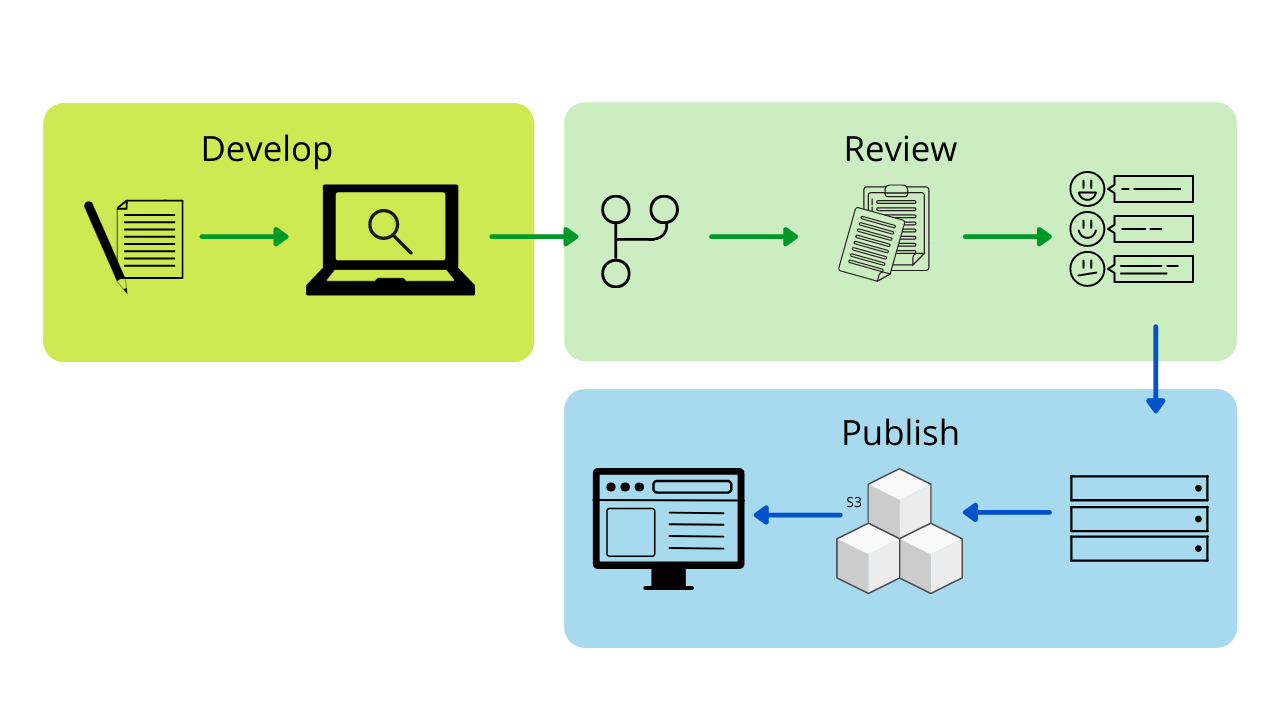
Here’s a brief overview of the process:
Create a dedicated docs folder in a Git repository.
Push Markdown files into the docs folder.
Configure the developer portal to publish docs from the respective code repository.
The latest version of the documentation will automatically be built and published in the developer portal.
Simplified documentation process
This way, technical documentation is closer to the source code and integrated into the code development process. Writing and updating technical documentation becomes part of writing code, and this encourages engineers to keep documentation updated.
Measuring success
Whenever there’s a change throughout big organisations like Grab, it can be tough to implement. But thankfully, our engineers recognised the importance of improving documentation and making it easier to maintain or update.
We surveyed our users and here’s what some have said about our Docs-as-Code initiative:
“[W]ith the doc and source code in one place, test backend engineers can now make doc changes via standard code review process and re-use the same content for CLI helper message and documentation.” – Kang Yaw Ong, Test Automation – Engineering Manager
“[Docs-as-Code] is a great initiative, as it keeps documentation in line and up-to-date with the development of a project. Managing documentation using a version control system and the same tools to handle merges and conflicts reduces overhead and friction in an engineer’s workflow.” – Eugene Chiang, Foundations – Engineering Manager
Progress and future optimisations
Since we first started the Docs-as-Code initiative in Grab, we’ve made a lot of progress in terms of adoption – approximately 80% of Grab services will have their technical documentation on the internal portal by April 2022.
We’ve also improved overall user experience by enhancing stability and performance, improving navigation and content formatting, and enabling feedback. But it doesn’t stop there; we are continuously improving the internal portal and providing more features for our engineers.
Apart from technical documentation, we are also applying the Docs-as-Code approach to our technical training content. This means moving both self-paced and workshop training content to a centralised repository and providing engineers a single platform for all their learning needs.
Special thanks to the Tech Learning – Documentation team for their contributions to this blog post.
We are hiring!
We are looking for more technical content developers to join the team. If you’re keen on joining our Docs-as-Code journey and improving developer experience, check out our open listings in Singapore and Malaysia.
Join us in driving this initiative forward and making documentation more approachable for everyone!
Join us
Grab is the leading superapp platform in Southeast Asia, providing everyday services that matter to consumers. More than just a ride-hailing and food delivery app, Grab offers a wide range of on-demand services in the region, including mobility, food, package and grocery delivery services, mobile payments, and financial services across 428 cities in eight countries.
Powered by technology and driven by heart, our mission is to drive Southeast Asia forward by creating economic empowerment for everyone. If this mission speaks to you, join our team today!
As a leading superapp in Southeast Asia, Grab serves millions of consumers daily. This naturally makes us a target for fraudsters and to enhance our defences, the Integrity team at Grab has launched several hyper-scaled services, such as the Griffin real-time rule engine and Advanced Feature Engineering. These systems enable data scientists and risk analysts to develop real-time scoring, and take fraudsters out of our ecosystems.
Apart from individual fraudsters, we have also observed the fast evolution of the dark side over time. We have had to evolve our defences to deal with professional syndicates that use advanced equipment such as device farms and GPS spoofing apps to perform fraud at scale. These professional fraudsters are able to camouflage themselves as normal users, making it significantly harder to identify them with rule-based detection.
Since 2020, Grab’s Integrity team has been advancing fraud detection with more sophisticated techniques and experimenting with a range of graph network technologies such as graph visualisations, graph neural networks and graph analytics. We’ve seen a lot of progress in this journey and will be sharing some key learnings that might help other teams who are facing similar issues.
What are Graph-based Prediction Platforms?
“You can fool some of the people all of the time, and all of the people some of the time, but you cannot fool all of the people all of the time.” – Abraham Lincoln
A Graph-based Prediction Platform connects multiple entities through one or more common features. When such entities are viewed as a macro graph network, we uncover new patterns that are otherwise unseen to the naked eye. For example, when investigating if two users are sharing IP addresses or devices, we might not be able to tell if they are fraudulent or just family members sharing a device.
However, if we use a graph system and look at all users sharing this device or IP address, it could show us if these two users are part of a much larger syndicate network in a device farming operation. In operations like these, we may see up to hundreds of other fake accounts that were specifically created for promo and payment fraud. With graphs, we can identify fraudulent activity more easily.
Grab’s Graph-based Prediction Platform
Leveraging the power of graphs, the team has primarily built two types of systems:
Graph Database Platform: An ultra-scalable storage system with over one billion nodes that powers:
Graph Visualisation: Risk specialists and data analysts can review user connections real-time and are able to quickly capture new fraud patterns with over 10 dimensions of features (see Fig 1).
Fig 1: Graph visualisation
Network-based feature system: A configurable system for engineers to adjust machine learning features based on network connectivity, e.g. number of hops between two users, numbers of shared devices between two IP addresses.
Graph-based Machine Learning: Unlike traditional fraud detection models, Graph Neural Networks (GNN) are able to utilise the structural correlations on the graph and act as a sustainable foundation to combat many different kinds of fraud. The data science team has built large-scale GNN models for scenarios like anti-money laundering and fraud detection.
Fig 2 shows a Money Laundering Network where hundreds of accounts coordinate the placement of funds, layering the illicit monies through a complex web of transactions making funds hard to trace, and consolidate funds into spending accounts.
Fig 2: Money Laundering Network
What’s next?
In the next article of our Graph Network blog series, we will dive deeper into how we develop the graph infrastructure and database using AWS Neptune. Stay tuned for the next part.
Join us
Grab is the leading superapp platform in Southeast Asia, providing everyday services that matter to consumers. More than just a ride-hailing and food delivery app, Grab offers a wide range of on-demand services in the region, including mobility, food, package and grocery delivery services, mobile payments, and financial services across 428 cities in eight countries.
Powered by technology and driven by heart, our mission is to drive Southeast Asia forward by creating economic empowerment for everyone. If this mission speaks to you, join our team today!
This article illustrates how the Cauldron Machine Learning (ML) Platform team uses GitLab parent-child pipelines to dynamically generate GitLab CI files to solve several limitations of GitLab for large repositories, namely:
Limitations to the number of includes (100 by default).
Simplifying the GitLab CI file from 1800 lines to 50 lines.
Reducing the need for nested gitlab-ci yml files.
Introduction
Cauldron is the Machine Learning (ML) Platform team at Grab. The Cauldron team provides tools for ML practitioners to manage the end to end lifecycle of ML models, from training to deployment. GitLab and its tooling are an integral part of our stack, for continuous delivery of machine learning.
One of our core products is MerLin Pipelines. Each team has a dedicated repo to maintain the code for their ML pipelines. Each pipeline has its own subfolder. We rely heavily on GitLab rules to detect specific changes to trigger deployments for the different stages of different pipelines (for example, model serving with Catwalk, and so on).
Background
Approach 1: Nested child files
Our initial approach was to rely heavily on static code generation to generate the child gitlab-ci.yml files in individual stages. See Figure 1 for an example directory structure. These nested yml files are pre-generated by our cli and committed to the repository.
Figure 1: Example directory structure with nested gitlab-ci.yml files.
Child gitlab-ci.yml files are added by using the include keyword.
Figure 2: Example root .gitlab-ci.yml file, and include clauses.
Figure 3: Example child `.gitlab-ci.yml` file for a given stage (Deploy Model) in a pipeline (pipeline 1).
As teams add more pipelines and stages, we soon hit a limitation in this approach:
There was a soft limit in the number of includes that could be in the base .gitlab-ci.yml file.
It became evident that this approach would not scale to our use-cases.
Approach 2: Dynamically generating a big CI file
Our next attempt to solve this problem was to try to inject and inline the nested child gitlab-ci.yml contents into the root gitlab-ci.yml file, so that we no longer needed to rely on the in-built GitLab “include” clause.
To achieve it, we wrote a utility that parsed a raw gitlab-ci file, walked the tree to retrieve all “included” child gitlab-ci files, and to replace the includes to generate a final big gitlab-ci.yml file.
Figure 4 illustrates the resulting file is generated from Figure 3.
Figure 4: “Fat” YAML file generated through this approach, assumes the original raw file of Figure 3.
This approach solved our issues temporarily. Unfortunately, we ended up with GitLab files that were up to 1800 lines long. There is also a soft limit to the size of gitlab-ci.yml files. It became evident that we would eventually hit the limits of this approach.
Solution
Our initial attempt at using static code generation put us partially there. We were able to pre-generate and infer the stage and pipeline names from the information available to us. Code generation was definitely needed, but upfront generation of code had some key limitations, as shown above. We needed a way to improve on this, to somehow generate GitLab stages on the fly. After some research, we stumbled upon Dynamic Child Pipelines.
Quoting the official website:
Instead of running a child pipeline from a static YAML file, you can define a job that runs your own script to generate a YAML file, which is then used to trigger a child pipeline.
This technique can be very powerful in generating pipelines targeting content that changed or to build a matrix of targets and architectures.
We were already on the right track. We just needed to combine code generation with child pipelines, to dynamically generate the necessary stages on the fly.
Architecture details
Figure 5: Flow diagram of how we use dynamic yaml generation. The user raises a merge request in a branch, and subsequently merges the branch to master.
Implementation
The user Git flow can be seen in Figure 5, where the user modifies or adds some files in their respective Git team repo. As a refresher, a typical repo structure consists of pipelines and stages (see Figure 1). We would need to extract the information necessary from the branch environment in Figure 5, and have a stage to programmatically generate the proper stages (for example, Figure 3).
In short, our requirements can be summarized as:
Detecting the files being changed in the Git branch.
Extracting the information needed from the files that have changed.
Passing this to be templated into the necessary stages.
Let’s take a very simple example, where a user is modifying a file in stage_1 in pipeline_1 in Figure 1. Our desired output would be:
Figure 6: Desired output that should be dynamically generated.
Our template would be in the form of:
Figure 7: Example template, and information needed. Let’s call it template_file.yml.
First, we need to detect the files being modified in the branch. We achieve this with native git diff commands, checking against the base of the branch to track what files are being modified in the merge request. The output (let’s call it diff.txt) would be in the form of:
M pipelines/pipeline_1/stage_1/modelserving.yaml
Figure 8: Example diff.txt generated from git diff.
We must extract the yellow and green information from the line, corresponding to pipeline_name and stage_name.
Figure 9: Information that needs to be extracted from the file.
We take a very simple approach here, by introducing a concept called stop patterns.
Stop patterns are defined as a comma separated list of variable names, and the words to stop at. The colon (:) denotes how many levels before the stop word to stop.
For example, the stop pattern:
pipeline_name:pipelines
tells the parser to look for the folder pipelines and stop before that, extracting pipeline_1 from the example above tagged to the variable name pipeline_name.
The stop pattern with two colons (::):
stage_name::pipelines
tells the parser to stop two levels before the folder pipelines, and extract stage_1 as stage_name.
Our cli tool allows the stop patterns to be comma separated, so the final command would be:
We elected to write the util in Rust due to its high performance, and its rich templating libraries (for example, Tera) and decent cli libraries (clap).
Combining all these together, we are able to extract the information needed from git diff, and use stop patterns to extract the necessary information to be passed into the template. Stop patterns are flexible enough to support different types of folder structures.
Figure 10: Example Rust code snippet for parsing the Git diff file.
When triggering pipelines in the master branch (see right side of Figure 5), the flow is the same, with a small caveat that we must retrieve the same diff.txt file from the source branch. We achieve this by using the rich GitLab API, retrieving the pipeline artifacts and using the same util above to generate the necessary GitLab steps dynamically.
Impact
After implementing this change, our biggest success was reducing one of the biggest ML pipeline Git repositories from 1800 lines to 50 lines. This approach keeps the size of the .gitlab-ci.yaml file constant at 50 lines, and ensures that it scales with however many pipelines are added.
Our users, the machine learning practitioners, also find it more productive as they no longer need to worry about GitLab yaml files.
Learnings and conclusion
With some creativity, and the flexibility of GitLab Child Pipelines, we were able to invest some engineering effort into making the configuration re-usable, adhering to DRY principles.
Grab is the leading superapp platform in Southeast Asia, providing everyday services that matter to consumers. More than just a ride-hailing and food delivery app, Grab offers a wide range of on-demand services in the region, including mobility, food, package and grocery delivery services, mobile payments, and financial services across 428 cities in eight countries.
Powered by technology and driven by heart, our mission is to drive Southeast Asia forward by creating economic empowerment for everyone. If this mission speaks to you, join our team today!
To build a NoOps managed streaming platform in Grab, the Coban team has:
Engineered an ecosystem on top of Apache Kafka.
Successfully adopted it to production for both transactional and analytical use cases.
Made it a battle-tested industrial-standard platform.
In 2021, the Coban team embarked on a new journey (Kafka Connect) that enables and empowers Grabbers to move data in and out of Apache Kafka seamlessly and conveniently.
Kafka Connect stack in Grab
This is what Coban’s Kafka Connect stack looks like today. Multiple data sources and data sinks, such as MySQL, S3 and Azure Data Explorer, have already been supported and productionised.
The Coban team has been using Protobuf as the serialisation-deserialisation (SerDes) format in Kafka. Therefore, the role of Confluent schema registry (shown at the top of the figure) is crucial to the Kafka Connect ecosystem, as it serves as the building block for conversions such as Protobuf-to-Avro, Protobuf-to-JSON and Protobuf-to-Parquet.
What problems are we trying to solve?
Problem 1: Change Data Capture (CDC)
In a big organisation like Grab, we handle large volumes of data and changes across many services on a daily basis, so it is important for these changes to be reflected in real time.
In addition, there are other technical challenges to be addressed:
As shown in the figure below, data is written twice in the code base – once into the database (DB) and once as a message into Kafka. In order for the data in the DB and Kafka to be consistent, the two writes have to be atomic in a two-phase commit protocol (or other atomic commitment protocols), which is non-trivial and impacts availability.
Some use cases require data both before and after a change.
Problem 2: Message mirroring for disaster recovery
The Coban team has done some research on Kafka MirrorMaker, an open-source solution. While it can ensure better data consistency, it takes significant effort to adopt it onto existing Kubernetes infrastructure hosted by the Coban team and achieve high availability.
Another major challenge that the Coban team faces is offset mirroring and translation, which is a known challenge in Kafka communities. In order for Kafka consumers to seamlessly resume their work with a backup Kafka after a disaster, we need to cater for offset translation.
Data ingestion into Azure Event Hubs
Azure Event Hubs has a Kafka-compatible interface and natively supports JSON and Avro schema. The Coban team uses Protobuf as the SerDes framework, which is not supported by Azure Event Hubs. It means that conversions have to be done for message ingestion into Azure Event Hubs.
Solution
To tackle these problems, the Coban team has picked Kafka Connect because:
It is an open-source framework with a relatively big community that we can consult if we run into issues.
It has the ability to plug in transformations and custom conversion logic.
Let us see how Kafka Connect can be used to resolve the previously mentioned problems.
Kafka Connect with Debezium connectors
Debezium is a framework built for capturing data changes on top of Apache Kafka and the Kafka Connect framework. It provides a series of connectors for various databases, such as MySQL, MongoDB and Cassandra.
Here are the benefits of MySQL binlog streams:
They not only provide changes on data, but also give snapshots of data before and after a specific change.
Some producers no longer have to push a message to Kafka after writing a row to a MySQL database. With Debezium connectors, services can choose not to deal with Kafka and only handle MySQL data stores.
Architecture
In case of DB upgrades and outages
DB Data Definition Language (DDL) changes, migrations, splits and outages are common in database operations, and each operation type has a systematic resolution.
The Debezium connector has built-in features to handle DDL changes made by DB migration tools, such as pt-online-schema-change, which is used by the Grab DB Ops team.
To deal with MySQL instance changes and database splits, the Coban team leverages on the Kafka Connect framework’s ability to change the offsets of connectors. By changing the offsets, Debezium connectors can properly function after DB migrations and resume binlog synchronisation from any position in any binlog file on a MySQL instance.
The CDC project on MySQL via Debezium connectors has been greatly successful in Grab. One of the biggest examples is its adoption in the Elasticsearch optimisation carried out by GrabFood, which has been published in another blog.
MirrorMaker2 with offset translation
Kafka MirrorMaker2 (MM2), developed in and shipped together with the Apache Kafka project, is a utility to mirror messages and consumer offsets. However, in the Coban team, the MM2 stack is deployed on the Kafka Connect framework per connector because:
A few Kafka Connect clusters have already been provisioned.
Compared to launching three connectors bundled in MM2, Coban can have finer controls on MirrorSourceConnector and MirrorCheckpointConnector, and manage both of them in an infrastructure-as-code way via Hashicorp Terraform.
Success stories
Ensuring business continuity is a key priority for Grab and this includes the ability to recover from incidents quickly. In 2021H2, there was a campaign that ran across many teams to examine the readiness and robustness of various services and middlewares. Coban’s Kafka is one of these services that proved to be robust after rounds of chaos engineering. With MM2 on Kafka Connect to mirror both messages and consumer offsets, critical services and pipelines could safely be replicated and launched across AWS regions if outages occur.
Because the Coban team has proven itself as the battle-tested Kafka service provider in Grab, other teams have also requested to migrate streams from self-managed Kafka clusters to ones managed by Coban. MM2 has been used in such migrations and brought zero downtime to the streams’ producers and consumers.
Mirror to Azure Event Hubs with an in-house converter
The Analytics team runs some real time ingestion and analytics projects on Azure. To support this cross-cloud use case, the Coban team has adopted MM2 for message mirroring to Azure Event Hubs.
Typically, Event Hubs only accept JSON and Avro bytes, which is incompatible with the existing SerDes framework. The Coban team has developed a custom converter that converts bytes serialised in Protobuf to JSON bytes at runtime.
These steps explain how the converter works:
Deserialise bytes in Kafka to a Protobuf DynamicMessage according to a schema retrieved from the Confluent™ schema registry.
Perform a recursive post-order depth-first-search on each field descriptor in the DynamicMessage.
Convert every Protobuf field descriptor to a JSON node.
Serialise the root JSON node to bytes.
The converter has not been open sourced yet.
Deployment
Docker containers are the Coban team’s preferred infrastructure, especially since some production Kafka clusters are already deployed on Kubernetes. The long-term goal is to provide Kafka in a software-as-a-service (SaaS) model, which is why Kubernetes was picked. The diagram below illustrates how Kafka Connect clusters are built and deployed.
What’s next?
The Coban team is iterating on a unified control plane to manage resources like Kafka topics, clusters and Kafka Connect. In the foreseeable future, internal users should be able to provision Kafka Connect connectors via RESTful APIs and a graphical user interface (GUI).
At the same time, the Coban team is closely working with the Data Engineering team to make Kafka Connect the preferred tool in Grab for moving data in and out of external storages (S3 and Apache Hudi).
Coban is hiring!
The Coban (Real-time Data Platform) team at Grab in Singapore is hiring software and site reliability engineers at all levels as we double down on growing our platform capabilities.
Join us in building state-of-the-art, mission critical, TB/hour scale data platforms that enable thousands of engineers, data scientists, and analysts to serve millions of consumers, businesses, and partners across Southeast Asia!
Join us
Grab is a leading superapp in Southeast Asia, providing everyday services that matter to consumers. More than just a ride-hailing and food delivery app, Grab offers a wide range of on-demand services in the region, including mobility, food, package and grocery delivery services, mobile payments, and financial services across over 400 cities in eight countries.
Powered by technology and driven by heart, our mission is to drive Southeast Asia forward by creating economic empowerment for everyone. If this mission speaks to you, join our team today!
At Grab, we run large marketing campaigns every day. A typical campaign may require executing multiple actions for millions of users all at once. The actions may include sending rewards, awarding points, and sending messages. Here is what a campaign may look like: On 1st Jan 2022, send two ride rewards to all the users in the “heavy users” segment. Then, send them a congratulatory message informing them about the reward.
Years ago, Grab’s marketing team used to stay awake at midnight to manually trigger such campaigns. They would upload a file at 12 am and then wait for a long time for the campaign execution to complete. To solve this pain point and support more capabilities down this line, we developed a “batch job” service, which is part of our in-house real-time automation engine, Trident.
The following are some services we use to support Grab’s marketing teams:
Rewards: responsible for managing rewards.
Messaging: responsible for sending messages to users. For example, push notifications.
Segmentation: responsible for storing and retrieving segments of users based on certain criteria.
For simplicity, only the services above will be referenced for this article. The “batch job” service we built uses rewards and messaging services for executing actions, and uses the segmentation service for fetching users in a segment.
System requirements
Functional requirements
Apply a sequence of actions targeting a large segment of users at a scheduled time, display progress to the campaign manager and provide a final report.
For each user, the actions must be executed in sequence; the latter action can only be executed if the preceding action is successful.
Non-functional requirements
Quick execution and high turnover rate.
Definition of turnover rate: the number of scheduled jobs completed per unit time.
Maximise resource utilisation and balance server load.
For the sake of brevity, we will not cover the scheduling logic, nor the generation of the report. We will focus specifically on executing actions.
Naive approach
Let’s start thinking from the most naive solution, and improve from there to reach an optimised solution.
Here is the pseudocode of a naive action executor.
def executeActionOnSegment(segment, actions):
   for user in fetchUsersInSegment(segment):
       for action in actions:
           success := doAction(user, action)
           if not success:
               break
           recordActionResult(user, action)

def doAction(user, action):
   if action.type == "awardReward":
       rewardService.awardReward(user, action.meta)
   elif action.type == "sendMessage":
       messagingService.sendMessage(user, action.meta)
   else:
       # other action types ...
One may be able to quickly tell that the naive solution does not satisfy our non-functional requirements for the following reasons:
Execution is slow:
The programme is single-threaded.
Actions are executed for users one by one in sequence.
Each call to the rewards and messaging services will incur network trip time, which impacts time cost.
Resource utilisation is low: The actions will only be executed on one server. When we have a cluster of servers, the other servers will sit idle.
Here are our alternatives for fixing the above issues:
Actions for different users should be executed in parallel.
API calls to other services should be minimised.
Distribute the work of executing actions evenly among different servers.
Note: Actions for the same user have to be executed in sequence. For example, if a sequence of required actions are (1) award a reward, (2) send a message informing the user to use the reward, then we can only execute action (2) after action (1) is successfully done for logical reasons and to avoid user confusion.
Our approach
A message queue is a well-suited solution to distribute work among multiple servers. We selected Kafka, among numerous message services, due to its following characteristics:
High throughput: Kafka can accept reads and writes at a very high speed.
Robustness: Events in Kafka are distributedly stored with redundancy, without a need to worry about data loss.
Pull-based consumption: Consumers can consume events at their own speed. This helps to avoid overloading our servers.
When a scheduled campaign is triggered, we retrieve the users from the segment in batches; each batch comprises around 100 users. We write the batches into a Kafka stream, and all our servers consume from the stream to execute the actions for the batches. The following diagram illustrates the overall flow.
Data in Kafka is stored in partitions. The partition configuration is important to ensure that the batches are evenly distributed among servers:
Number of partitions: Ensure that the number of stream partitions is greater than or equal to the max number of servers we will have in our cluster. This is because one Kafka partition can only be consumed by one consumer. If we have more consumers than partitions, some consumers will not receive any data.
Partition key: For each batch, assign a hash value as the partition key to randomly allocate batches into different partitions.
Now that work is distributed among servers in batches, we can consider how to process each batch faster. If we follow the naive logic, for each user in the batch, we need to call the rewards or messaging service to execute the actions. This will create very high QPS (queries per second) to those services, and incur significant network round trip time.
To solve this issue, we decided to build batch endpoints in rewards and messaging services. Each batch endpoint takes in a list of user IDs and action metadata as input parameters, and returns the action result for each user, regardless of success or failure. With that, our batch processing logic looks like the following:
In the implementation of batch endpoints, we also made optimisations to reduce latency. For example, when awarding rewards, we need to write the records of a reward being given to a user in multiple database tables. If we make separate DB queries for each user in the batch, it will cause high QPS to DB and incur high network time cost. Therefore, we grouped all the users in the batch into one DB query for each table update instead.
Benchmark tests show that using the batch DB query reduced API latency by up to 85%.
Further optimisations
As more campaigns started running in the system, we came across various bottlenecks. Here are the optimisations we implemented for some major examples.
Shard stream by action type
Two widely used actions are awarding rewards and sending messages to users. We came across situations where the sending of messages was blocked because a different campaign of awarding rewards had already started. If millions of users were targeted for rewards, this could result in significant waiting time before messages are sent, ultimately leading them to become irrelevant.
We found out the API latency of awarding rewards is significantly higher than sending messages. Hence, to make sure messages are not blocked by long-running awarding jobs, we created a dedicated Kafka topic for messages. By having different Kafka topics based on the action type, we were able to run different types of campaigns in parallel.
Shard stream by country
Grab operates in multiple countries. We came across situations where a campaign of awarding rewards to a small segment of users in one country was delayed by another campaign that targeted a huge segment of users in another country. The campaigns targeting a small set of users are usually more time-sensitive.
Similar to the above solution, we added different Kafka topics for each country to enable the processing of campaigns in different countries in parallel.
Remove unnecessary waiting
We observed that in the case of chained actions, messaging actions are generally the last action in the action list. For example, after awarding a reward, a congratulatory message would be sent to the user.
We realised that it was not necessary to wait for a sending message action to complete before processing the next batch of users. Moreover, the latency of the sending messages API is lower than awarding rewards. Hence, we adjusted the sending messages API to be asynchronous, so that the task of awarding rewards to the next batch of users can start while messages are being sent to the previous batch.
Conclusion
We have architected our batch jobs system in such a way so that it can be enhanced and optimised without redoing its work. For example, although we currently obtain the list of targeted users from a segmentation service, in the future, we may obtain this list from a different source, for example, all Grab Platinum tier members.
Join us
Grab is a leading superapp in Southeast Asia, providing everyday services that matter to consumers. More than just a ride-hailing and food delivery app, Grab offers a wide range of on-demand services in the region, including mobility, food, package and grocery delivery services, mobile payments, and financial services across over 400 cities in eight countries.
Powered by technology and driven by heart, our mission is to drive Southeast Asia forward by creating economic empowerment for everyone. If this mission speaks to you, join our team today!
Telematics is a collection of sensor data such as accelerometer data, gyroscope data, and GPS data that a driver’s mobile phone provides, and we collect, during the ride. With this information, we apply data science logic to detect traffic events such as harsh braking, acceleration, cornering, and unsafe lane changes, in order to help improve our consumers’ ride experience.
Introduction
As Grab grows to meet our consumers’ needs, the number of driver-partners has also grown. This requires us to ensure that our consumers’ safety continues to remain the highest priority as we scale. We developed an in-house telematics engine which uses mobile phone sensors to determine, evaluate, and quantify the driving behaviour of our driver-partners. This telemetry data is then evaluated and gives us better insights into our driver-partners’ driving patterns.
Through our data, we hope to improve our driver-partners’ driving habits and reduce the likelihood of driving-related incidents on our platform. This telemetry data also helps us determine optimal insurance premiums for driver-partners with risky driving patterns and reward driver-partners who have better driving habits.
In addition, we also merge telematics data with spatial data to further identify areas where dangerous driving manoeuvres happen frequently. This data is used to inform our driver-partners to be alert and drive more safely in such areas.
Background
With more consumers using the Grab app, we realised that purely relying on passenger feedback is not enough; we had no definitive way to tell which driver-partners were actually driving safely, when they deviated from their routes or even if they had been involved in an accident.
To help address these issues, we developed an in-house telematics engine that analyses telemetry data, identifies driver-partners’ driving behaviour and habits, and provides safety reports for them.
Architecture details
As shown in the diagram, our telematics SDK receives raw sensor data from our driver-partners’ devices and processes it in two ways:
On-device processing for crash detection: Used to determine situations such as if the driver-partner has been in an accident.
Raising traffic events and generating safety reports after each job: Useful for detecting events like speeding and harsh braking.
Note: Safety reports are generated by our backend service using sensor data that is only uploaded as a text file after each ride.
Implementation
Our telematics framework relies on accelerometer, gyroscope and GPS sensors within the mobile device to infer the vehicle’s driving parameters. Both accelerometer and gyroscope are triaxial sensors, and their respective measurements are in the mobile device’s frame of reference.
That being said, the data collected from these sensors have no fixed sample rate, so we need to implement sensor data time synchronisation. For example, there will be temporal misalignment between gyroscope and accelerometer data if they do not share the same timestamp. The sample rate that comes from the accelerometer and gyroscope also varies independently. Therefore, we need to uniformly sample the sensor data to be at the same frequency rate.
This synchronisation process is done in two steps:
Interpolation to uniform time grid at a reasonably higher frequency.
Decimation from the higher frequency to the output data rate for accelerometer and gyroscope data.
We then use the Fourier Transform to transform a signal from time domain to frequency domain for compression. These components are then written to a text file on the mobile device, compressed, and uploaded after the end of each ride.
Learnings/Conclusion
There are a few takeaways that we learned from this project:
Sensor data frequency: There are many device manufacturers out there for Android and each one of them has a different sensor chipset. The frequency of the sensor data may vary from device to device.
Four-wheel (4W) vs two-wheel (2W): The behaviour is different for a driver-partner on 2W vs 4W, so we need different rules for each.
Hardware axis-bias: The device may not be aligned with the vehicle during the ride. It cannot be assumed that the phone will remain in a fixed orientation throughout the trip, so the mobile device sensors might not accurately measure the acceleration/braking or sharp turning of the vehicle.
Sensor noise: There are artifacts in sensor readings, which are basically a single outlier event that represents an error and is not a valid sensor reading.
Time-synchronisation: GPS, accelerometer, and gyroscope events are captured independently by three different sensors and have different time formats. These events will need to be transformed into the same time grid in order to work together. For example, the GPS location from 30 seconds prior to the gyroscope event will not work as they are out of sync.
Data compression and network consumption: Longer rides will contain more telematics data. It will result in a bigger upload size and increase in time for file compression.
What’s next?
There are a few milestones that we want to accomplish with our telematics framework in the future. However, our number one goal is to extend telematics to all bookings across Grab verticals. We are also planning to add more on-device rules and data processing for event detections to further eliminate future delays from backend communication for crash detection.
With the data from our telematics framework, we can improve our passengers’ experience and improve safety for both passengers and driver-partners.
Join us
Grab is a leading superapp in Southeast Asia, providing everyday services that matter to consumers. More than just a ride-hailing and food delivery app, Grab offers a wide range of on-demand services in the region, including mobility, food, package and grocery delivery services, mobile payments, and financial services across over 400 cities in eight countries.
Powered by technology and driven by heart, our mission is to drive Southeast Asia forward by creating economic empowerment for everyone. If this mission speaks to you, join our team today!
Typically, modern applications use various database engines for their service needs; within Grab, these would be MySQL, Aurora and DynamoDB. Lately, the Caspian team has observed an increasing need to consume real-time data for many service teams. These real-time changes in database records help to support online and offline business decisions for hundreds of teams.
Because of that, we have invested time into synchronising data from MySQL, Aurora and Dynamodb to the message queue, i.e. Kafka. In this blog, we share how real-time data ingestion has helped since it was launched.
Introduction
Over the last few years, service teams had to write all transactional data twice: once into Kafka and once into the database. This helped to solve the inter-service communication challenges and obtain audit trail logs. However, if the transactions fail, data integrity becomes a prominent issue. Moreover, it is a daunting task for developers to maintain the schema of data written into Kafka.
With real-time ingestion, there is a notably better schema evolution and guaranteed data consistency; service teams no longer need to write data twice.
You might be wondering, why don’t we have a single transaction that spans the services’ databases and Kafka, to make data consistent? This would not work as Kafka does not support being enlisted in distributed transactions. In some situations, we might end up having new data persisting into the services’ databases, but not having the corresponding message sent to Kafka topics.
Instead of registering or modifying the mapped table schema in Golang writer into Kafka beforehand, service teams tend to avoid such schema maintenance tasks entirely. In such cases, real-time ingestion can be adopted where data exchange among the heterogeneous databases or replication between source and replica nodes is required.
While reviewing the key challenges around real-time data ingestion, we realised that there were many potential user requirements to include. To build a standardised solution, we identified several points that we felt were high priority:
Make transactional data readily available in real time to drive business decisions at scale.
Capture audit trails of any given database.
Get rid of the burst read on databases caused by SQL-based query ingestion.
To empower Grabbers with real-time data to drive their business decisions, we decided to take a scalable event-driven approach, which is being facilitated with a bunch of internal products, and designed a solution for real-time ingestion.
Anatomy of architecture
The solution for real-time ingestion has several key components:
Stream data storage
Event producer
Message queue
Stream processor
Figure 1. Real time ingestion architecture
Stream storage
Stream storage acts as a repository that stores the data transactions in order with exactly-once guarantee. However, the level of order in stream storage differs with regards to different databases.
For MySQL or Aurora, transaction data is stored in binlog files in sequence and rotated, thus ensuring global order. Data with global order assures that all MySQL records are ordered and reflects the real life situation. For example, when transaction logs are replayed or consumed by downstream consumers, consumer A’s Grab food order at 12:01:44 pm will always appear before consumer B’s order at 12:01:45 pm.
However, this does not necessarily hold true for DynamoDB stream storage as DynamoDB streams are partitioned. Audit trails of a given record show that they go into the same partition in the same order, ensuring consistent partitioned order. Thus when replay happens, consumer B’s order might appear before consumer A’s.
Moreover, there are multiple formats to choose from for both MySQL binlog and DynamoDB stream records. We eventually set ROW for binlog formats and NEW_AND_OLD_IMAGES for DynamoDB stream records. This depicts the detailed information before and after modifying any given table record. The binlog and DynamoDB stream main fields are tabulated in Figures 2 and 3 respectively.
Figure 2. Binlog record schema
Figure 3. DynamoDB stream record schema
Event producer
Event producers take in binlog messages or stream records and output to the message queue. We evaluated several technologies for the different database engines.
For MySQL or Aurora, three solutions were evaluated: Debezium, Maxwell, and Canal. We chose to onboard Debezium as it is deeply integrated with the Kafka Connect framework. Also, we see the potential of extending solutions among other external systems whenever moving large collections of data in and out of the Kafka cluster.
One such example is the open source project that attempts to build a custom DynamoDB connector extending the Kafka Connect (KC) framework. It self manages checkpointing via an additional DynamoDB table and can be deployed on KC smoothly.
However, the DynamoDB connector fails to exploit the fundamental nature of storage DynamoDB streams: dynamic partitioning and auto-scaling based on the traffic. Instead, it spawns only a single thread task to process all shards of a given DynamoDB table. As a result, downstream services suffer from data latency the most when write traffic surges.
In light of this, the lambda function becomes the most suitable candidate as the event producer. Not only does the concurrency of lambda functions scale in and out based on actual traffic, but the trigger frequency is also adjustable at your discretion.
Kafka
This is the distributed data store optimised for ingesting and processing data in real time. It is widely adopted due to its high scalability, fault-tolerance, and parallelism. The messages in Kafka are abstracted and encoded into Protobuf.
Stream processor
The stream processor consumes messages in Kafka and writes into S3 every minute. There are a number of options readily available in the market; Spark and Flink are the most common choices. Within Grab, we deploy a Golang library to deal with the traffic.
Use cases
Now that we’ve covered how real-time data ingestion is done in Grab, let’s look at some of the situations that could benefit from real-time data ingestion.
1. Data pipelines
We have thousands of pipelines running hourly in Grab. Some tables have significant growth and generate workload beyond what a SQL-based query can handle. An hourly data pipeline would incur a read spike on the production database shared among various services, draining CPU and memory resources. This deteriorates other services’ performance and could even block them from reading. With real-time ingestion, the query from data pipelines would be incremental and span over a period of time.
Another scenario where we switch to real-time ingestion is when a missing index is detected on the table. To speed up the query, SQL-based query ingestion requires indexing on columns such as created_at, updated_at and id. Without indexing, SQL based query ingestion would either result in high CPU and memory usage, or fail entirely.
Although adding indexes for these columns would resolve this issue, it comes with a cost, i.e. a copy of the indexed column and primary key is created on disk and the index is kept in memory. Creating and maintaining an index on a huge table is much costlier than for small tables. With performance consideration in mind, it is not recommended to add indexes to an existing huge table.
Instead, real-time ingestion overshadows SQL-based ingestion. We can spawn a new connector, archiver (Coban team’s Golang library that dumps data from Kafka at minutes-level frequency) and compaction job to bubble up the table record from binlog to the destination table in the Grab data lake.
Figure 4. Using real-time ingestion for data pipelines
2. Drive business decisions
A key use case of enabling real-time ingestion is driving business decisions at scale without even touching the source services. Saga pattern is commonly adopted in the microservice world. Each service has its own database, splitting an overarching database transaction into a series of multiple database transactions. Communication is established among services via message queue i.e. Kafka.
In an earlier tech blog published by the Grab Search team, we talked about how real-time ingestion with Debezium optimised and boosted search capabilities. Each MySQL table is mapped to a Kafka topic and one or multiple topics build up a search index within Elasticsearch.
With this new approach, there is no data loss, i.e. changes via MySQL command line tool or other DB management tools can be captured. Schema evolution is also naturally supported; the new schema defined within a MySQL table is inherited and stored in Kafka. No producer code change is required to make the schema consistent with that in MySQL. Moreover, the database read has been reduced by 90 percent including the efforts of the Data Synchronisation Platform.
Figure 5. Grab Search team use case
The GrabFood team exemplifies mostly similar advantages in the DynamoDB area. The only differences compared to MySQL are that the frequency of the lambda functions is adjustable and parallelism is auto-scaled based on the traffic. By auto-scaling, we mean that more lambda functions will be auto-deployed to cater to a sudden spike in traffic, or destroyed as the traffic falls.
Figure 6. Grab Food team use case
3. Database replication
Another use case we did not originally have in mind is incremental data replication for disaster recovery. Within Grab, we enable DynamoDB streams for tier 0 and critical DynamoDB tables. Any insert, delete, modify operations would be propagated to the disaster recovery table in another availability zone.
When migrating or replicating databases, we use the strangler fig pattern, which offers an incremental, reliable process for migrating databases. This is a method whereby a new system slowly grows on top of an old system and is gradually adopted until the old system is “strangled” and can simply be removed. Figure 7 depicts how DynamoDB streams drive real-time synchronisation between tables in different regions.
Figure 7. Data replication among DynamoDB tables across different regions in DBOps team
4. Deliver audit trails
Reasons for maintaining data audit trails are manifold in Grab: regulatory requirements might mandate businesses to keep complete historical information of a consumer or to apply machine learning techniques to detect fraudulent transactions made by consumers. Figure 8 demonstrates how we deliver audit trails in Grab.
Figure 8. Deliver audit trails in Grab
Summary
Real time ingestion is playing a pivotal role in Grab’s ecosystem. It:
boosts data pipelines with less read pressure imposed on databases shared among various services;
empowers real-time business decisions with assured resource efficiency;
provides data replication among tables residing in various regions; and
delivers audit trails that either keep complete history or help unearth fraudulent operations.
Since this project launched, we have made crucial enhancements to facilitate daily operations with several in-house products that are used for data onboarding, quality checking, maintaining freshness, etc.
We will continuously improve our platform to provide users with a seamless experience in data ingestion, starting with unifying our internal tools. Apart from providing a unified platform, we will also contribute more ideas to the ingestion, extending it to Azure and GCP, supporting multi-catalogue and offering multi-tenancy.
In our next blog, we will drill down to other interesting features of real-time ingestion, such as how ordering is achieved in different cases and custom partitioning in real-time ingestion. Stay tuned!
Join us
Grab is a leading superapp in Southeast Asia, providing everyday services that matter to consumers. More than just a ride-hailing and food delivery app, Grab offers a wide range of on-demand services in the region, including mobility, food, package and grocery delivery services, mobile payments, and financial services across over 400 cities in eight countries.
Powered by technology and driven by heart, our mission is to drive Southeast Asia forward by creating economic empowerment for everyone. If this mission speaks to you, join our team today!
Earlier in 2021 we published an article on Trident, Grab’s in-house real-time if this, then that (IFTTT) engine which manages campaigns for the Grab Loyalty Programme. The Grab Loyalty Programme encourages consumers to make Grab transactions by rewarding points when transactions are made. Grab rewards two types of points namely OVOPoints and GrabRewards Points (GRP). OVOPoints are issued for transactions made in Indonesia and GRP are for the transactions that are made in all other markets. In this article, the term GRP will be used to refer to both OVOPoints and GrabRewards Points.
Rewarding GRP is one of the main components of the Grab Loyalty Programme. By rewarding GRP, our consumers are incentivised to transact within the Grab ecosystem. Consumers can then redeem their GRP for a range of exciting items on the GrabRewards catalogue or to offset the cost of their spendings.
As we continue to grow our consumer base and our product offerings, a more robust platform is needed to ensure successful points transactions. In this post, we will share the challenges in rewarding GRP and how Abacus, our Point Issuance platform helps to overcome these challenges while managing various use cases.
Challenges
Growing number of products
The number of Grab’s product offerings has grown as part of Grab’s goal in becoming a superapp. The demand for rewarding GRP increased as each product team looked for ways to retain consumer loyalty. For this, we needed a platform which could support the different requirements from each product team.
External partnerships
Grab’s external partnerships consist of both one- and two-way point exchanges. With selected partners, Grab users are able to convert their GRP for the partner’s loyalty programme points, and the other way around.
Use cases
Besides the need to cater for the growing number of products and external partnerships, Grab needed a centralised points management system which could cater to various use cases of points rewarding. Let’s take a look at the use cases.
Any product, any points
There are many products in Grab and each product should be able to reward different GRP for different scenarios. Each product rewards GRP based on the goal they are trying to achieve.
The following examples illustrate the different scenarios:
GrabCar: Reward 100 GRP for when a driver cancels a booking as a form of compensation or to reward GRP for every ride a consumer makes.
GrabFood: Reward consumers for each meal order.
GrabPay: Reward consumers three times the number of GRP for using GrabPay instead of cash as the mode of payment.
More points for loyal consumers
Another use case is to reward loyal consumers with more points. This incentivises consumers to transact within the Grab ecosystem. One example are membership tiers granted based on the number of GRP a consumer has accumulated. There are four membership tiers: Member, Silver, Gold and Platinum.
Point multiplier
There are different points multipliers for different membership tiers. For example, a Gold member would earn 2.25 GRP for every dollar spent while a Silver member earns only 1.5 GRP for the same amount spent. A consumer can view their membership tier and GRP information from the account page on the Grab app.
GrabRewards Points and membership tier information
Growing number of transactions
Teams within Grab and external partners use GRP in their business. There is a need for a platform that can process millions of transactions every day with high availability rates. Errors can easily impact the issuance of points which may affect our consumers’ trust.
Our solution – Abacus
To overcome the challenges and cater for various use cases, we developed a Points Management System known as Abacus. It offers an interface for external partners with the capability to handle millions of daily transactions without significant downtime.
Points rewarding
There are seven main components of Abacus as shown in the following architectural diagram. Details of each component are explained in this section.
Abacus architecture
Transaction input source
The points rewarding process begins when a transaction is complete. Abacus listens to streams for completed transactions on the Grab platform. Each transaction that abacus receives in the stream carries the data required to calculate the GRP to be rewarded such as country ID, product ID, and payment ID etc.
Apart from computing the number of GRP to be rewarded for a transaction and then rewarding the points, Abacus also allows clients from within the Grab platform and outside of the Grab platform to make an API call to reward GRP to consumers. The client who wants to reward their consumers with GRP will call Abacus with either a specific point value (for example 100 points) or will provide the necessary details like transaction amount and the relevant multipliers for Abacus to compute the points and then reward them.
Point Calculation module
The Point Calculation module calculates the GRP using the data and multipliers that are unique to each transaction.
Point Calculation dependencies for internal services
Point Calculation dependencies are the multipliers needed to calculate the number of points. The Point Calculation module fetches the correct point multipliers for each transaction. The multipliers are configured by specific country teams when the product is launched. They may vary by country to allow country teams the flexibility to achieve their growth and retention targets. There are different types of multipliers.
Vertical multiplier: The multiplier for each vertical. A vertical is a service or product offered by Grab. Examples of verticals are GrabCar and GrabFood. The multiplier can be different for each vertical.
EPPF multiplier: The effective price per fare multiplier. EPPF is the reference conversion rate per point. For example:
EPPF = 1.0; if you are issuing X points per SGD1
EPPF = 0.1; if you are issuing X points per THB10
EPPF = 0.0001; if you are issuing X points per IDR10,000
Payment Type multiplier: The multiplier for different modes of payments.
Tier multiplier: The multiplier for each tier.
Point Calculation formula for internal clients
The Point Calculation module uses a formula to calculate GRP. The formula is the product of all the multipliers and the transaction amount.
Example of multipliers for payment options and tiers
Point Calculation dependencies for external clients
External partners supply the Point Calculation dependencies which are then configured in our backend at the time of integration. These external partners can set their own multipliers instead of using the above mentioned multipliers which are specific to Grab. This document details the APIs which are used to award points for external clients.
Simple Queue Service
Abacus uses Amazon Simple Queue Service (SQS) to ensure that the points system process is robust and fault tolerant.
Point Awarding SQS
If there are no errors during the Point Calculation process, the Point Calculation module will send a message containing the points to be awarded to the Point Awarding SQS.
Retry SQS
The Point Calculation module may not receive the required data when there is a downtime in the Point Calculation dependencies. If this occurs, an error is triggered and the Point Calculation module will send a message to Retry SQS. Messages sent to the Retry SQS will be re-processed by the Point Calculation module. This ensures that the points are properly calculated despite having outages on dependencies. Every message that we push to either the Point Awarding SQS or Retry SQS will have a field called Idempotency key which is used to ensure that we reward the points only once to a particular transaction.
Point Awarding module
The successful calculation of GRP triggers a message to the Point Awarding module via the Point SQS. The Point Awarding module tries to reward GRP to the consumer’s account. Upon successful completion, an ACK is sent back to the Point SQS signalling that the message was successfully processed and triggers deletion of the message. If Point SQS does not receive an ACK, the message is redelivered after an interval. This process ensures that the points system is robust and fault tolerant.
Ledger
GRP is rewarded to the consumer once it is updated in the Ledger. The Ledger tracks how many GRP a consumer has accumulated, what they were earned for, and the running total number of GRP.
Notification service
Once the Ledger is updated, the Notification service sends the consumer a message about the GRP they receive.
Point Kafka stream
For all successful GRP transactions, Abacus sends a message to the Point Kafka stream. Downstream services listen to this stream to identify the consumer’s behaviour and take the appropriate actions. Services of this stream can listen to events they are interested in and execute their business logic accordingly. For example, a service can use the information from the Point Kafka stream to determine a consumer’s membership tier.
Points expiry
Further addition to Abacus is the handling of points expiry. The Expiry Extension module enables activity-based points expiry. This enables GRP to not expire as long as the consumer makes one Grab transaction within the next three or six months from their last transaction.
The Expiry Extension module updates the point expiry date to the database after successfully rewarding GRP to the consumer. At the end of each month, a process loads all consumers whose points will expire in that particular month and sends it to the Point Expiry SQS. The Point Expiry Consumer will then expire all the points for the consumers and this data is updated in the Ledger. This process repeats on a monthly basis.
Expiry Extension module
Points expiry date is always the last day of the third or sixth month. For example, Adam makes a transaction on 10 January. His points expiry date is 31 July which is six months from the month of his last transaction. Adam then makes a transaction on 28 February. His points expiry period is shifted by one month to 31 August.
Points expiry
Conclusion
The Abacus platform enables us to perform millions of GRP transactions on a daily basis. Being able to curate rewards for consumers increases the value proposition of our products and consumer retention. If you have any comments or questions about Abacus, feel free to leave a comment below.
Special thanks to Arianto Wibowo and Vaughn Friesen.
Join us
Grab is a leading superapp in Southeast Asia, providing everyday services that matter to consumers. More than just a ride-hailing and food delivery app, Grab offers a wide range of on-demand services in the region, including mobility, food, package and grocery delivery services, mobile payments, and financial services across over 400 cities in eight countries.
Powered by technology and driven by heart, our mission is to drive Southeast Asia forward by creating economic empowerment for everyone. If this mission speaks to you, join our team today!
In large organisations, it is a common practice to isolate the cloud resources of different verticals. Amazon Web Services (AWS) Virtual Private Cloud (VPC) is a convenient way of doing so. At Grab, while our core AWS services reside in a main VPC, a number of Grab Tech Families (TFs) have their own dedicated VPC. One such example is GrabKios. Previously known as “Kudo”, GrabKios was acquired by Grab in 2017 and has always been residing in its own AWS account and dedicated VPC.
In this article, we explore how we exposed an Apache Kafka cluster across multiple Availability Zones (AZs) in Grab’s main VPC, to producers and consumers residing in the GrabKios VPC, via a VPC Endpoint Service. This design is part of Coban unified stream processing platform at Grab.
There are several ways of enabling communication between applications across distinct VPCs; VPC peering is the most straightforward and affordable option. However, it potentially exposes the entire VPC networks to each other, needlessly increasing the attack surface.
Security has always been one of Grab’s top concerns and with Grab’s increasing growth, there is a need to deprecate VPC peering and shift to a method of only exposing services that require remote access. The AWS VPC Endpoint Service allows us to do exactly that for TCP/IPv4 communications within a single AWS region.
Setting up a VPC Endpoint Service compared to VPC peering is already relatively complex. On top of that, we need to expose an Apache Kafka cluster via such an endpoint, which comes with an extra challenge. Apache Kafka requires clients, called producers and consumers, to be able to deterministically establish a TCP connection to all brokers forming the cluster, not just any one of them.
Last but not least, we need a design that optimises performance and cost by limiting data transfer across AZs.
Note: All variable names, port numbers and other details used in this article are only used as examples.
Architecture overview
As shown in this diagram, the Kafka cluster resides in the service provider VPC (Grab’s main VPC) while local Kafka producers and consumers reside in the service consumer VPC (GrabKios VPC).
In Grab’s main VPC, we created a Network Load Balancer (NLB) and set it up across all three AZs, enabling cross-zone load balancing. We then created a VPC Endpoint Service associated with that NLB.
Next, we created a VPC Endpoint Network Interface in the GrabKios VPC, also set up across all three AZs, and attached it to the remote VPC endpoint service in Grab’s main VPC. Apart from this, we also created a Route 53 Private Hosted Zone .grab and a CNAME record kafka.grab that points to the VPC Endpoint Network Interface hostname.
Lastly, we configured producers and consumers to use kafka.grab:10000 as their Kafka bootstrap server endpoint, 10000/tcp being an arbitrary port of our choosing. We will explain the significance of these in later sections.
Network Load Balancer setup
On the NLB in Grab’s main VPC, we set up the corresponding bootstrap listener on port 10000/tcp, associated with a target group containing all of the Kafka brokers forming the cluster. But this listener alone is not enough.
As mentioned earlier, Apache Kafka requires producers and consumers to be able to deterministically establish a TCP connection to all brokers. That’s why we created one listener for every broker in the cluster, incrementing the TCP port number for each new listener, so each broker endpoint would have the same name but with different port numbers, e.g. kafka.grab:10001 and kafka.grab:10002.
We then associated each listener with a dedicated target group containing only the targeted Kafka broker, so that remote producers and consumers could differentiate between the brokers by their TCP port number.
The following listeners and associated target groups were set up on the NLB:
In the Kafka brokers’ Security Group (SG), we added an ingress SG rule allowing 9094/tcp traffic from each of the three private IP addresses of the NLB. As mentioned earlier, the NLB was set up across all three AZs, with each having its own private IP address.
On the GrabKios VPC (consumer side), we created a new SG and attached it to the VPC Endpoint Network Interface. We also added ingress rules to allow all producers and consumers to connect to tcp/10000-10003.
Kafka setup
Kafka brokers typically come with a listener on port 9092/tcp, advertising the brokers by their private IP addresses. We kept that default listener so that local producers and consumers in Grab’s main VPC could still connect directly.
$ kcat -L -b 10.0.0.1:9092
 3 brokers:
 broker 101 at 10.0.0.1:9092 (controller)
 broker 201 at 10.0.0.2:9092
 broker 301 at 10.0.0.3:9092
... truncated output ...
We also configured all brokers with an additional listener on port 9094/tcp that advertises the brokers by:
Their shared private name kafka.grab.
Their distinct TCP ports previously set up on the NLB’s dedicated listeners.
$ kcat -L -b 10.0.0.1:9094
 3 brokers:
 broker 101 at kafka.grab:10001 (controller)
 broker 201 at kafka.grab:10002
 broker 301 at kafka.grab:10003
... truncated output ...
Note that there is a difference in how the broker’s endpoints are advertised in the two outputs above. The latter enables connection to any particular broker from the GrabKios VPC via the VPC Endpoint Service.
It would definitely be possible to advertise the brokers directly with the remote VPC Endpoint Interface hostname instead of kafka.grab, but relying on such a private name presents at least two advantages.
First, it decouples the Kafka deployment in the service provider VPC from the infrastructure deployment in the service consumer VPC. Second, it makes the Kafka cluster easier to expose to other remote VPCs, should we need it in the future.
Limiting data transfer across Availability Zones
At this stage of the setup, our Kafka cluster is fully reachable from producers and consumers in the GrabKios VPC. Yet, the design is not optimal.
When a producer or a consumer in the GrabKios VPC needs to connect to a particular broker, it uses its individual endpoint made up of the shared name kafka.grab and the broker’s dedicated TCP port.
The shared name arbitrarily resolves into one of the three IP addresses of the VPC Endpoint Network Interface, one for each AZ.
Hence, there is a fair chance that the obtained IP address is neither in the client’s AZ nor in that of the target Kafka broker. The probability of this happening can be as high as 2/3 when both client and broker reside in the same AZ and 1/3 when they do not.
While that is of little concern for the initial bootstrap connection, it becomes a serious drawback for actual data transfer, impacting the performance and incurring unnecessary data transfer cost.
For this reason, we created three additional CNAME records in the Private Hosted Zone in the GrabKios VPC, one for each AZ, with each pointing to the VPC Endpoint Network Interface zonal hostname in the corresponding AZ:
kafka-az1.grab
kafka-az2.grab
kafka-az3.grab
Note that we used az1, az2, az3 instead of the typical AWS 1a, 1b, 1c suffixes, because the latter’s mapping is not consistent across AWS accounts.
We also reconfigured each Kafka broker in Grab’s main VPC by setting their 9094/tcp listener to advertise brokers by their new zonal private names.
$ kcat -L -b 10.0.0.1:9094
 3 brokers:
 broker 101 at kafka-az1.grab:10001 (controller)
 broker 201 at kafka-az2.grab:10002
 broker 301 at kafka-az3.grab:10003
... truncated output ...
Our private zonal names are shared by all brokers in the same AZ while TCP ports remain distinct for each broker. However, this is not clearly shown in the output above because our cluster only counts three brokers, one in each AZ.
The previous common name kafka.grab remains in the GrabKios VPC’s Private Hosted Zone and allows connections to any broker via an arbitrary, likely non-optimal route. GrabKios VPC producers and consumers still use that highly-available endpoint to initiate bootstrap connections to the cluster.
Future improvements
For this setup, scalability is our main challenge. If we add a new broker to this Kafka cluster, we would need to:
Assign a new TCP port number to it.
Set up a new dedicated listener on that TCP port on the NLB.
Configure the newly spun up Kafka broker to advertise its service with the same TCP port number and the private zonal name corresponding to its AZ.
Add the new broker to the target group of the bootstrap listener on the NLB.
Update the network SG rules on the service consumer side to allow connections to the newly allocated TCP port.
We rely on Terraform to dynamically deploy all AWS infrastructure and on Jenkins and Ansible to deploy and configure Apache Kafka. There is limited overhead but there are still a few manual actions due to a lack of integration. These include transferring newly allocated TCP ports and their corresponding EC2 instances’ IP addresses to our Ansible inventory, commit them to our codebase and trigger a Jenkins job deploying the new Kafka broker.
Another concern of this setup is that it is only applicable for AWS. As we are aiming to be multi-cloud, we may need to port it to Microsoft Azure and leverage the Azure Private Link service.
In both cases, running Kafka on Kubernetes with the Strimzi operator would be helpful in addressing the scalability challenge and reducing our adherence to one particular cloud provider. We will explain how this solution has helped us address these challenges in a future article.
Special thanks to David Virgil Naranjo whose blog post inspired this work.
Join us
Grab is a leading superapp in Southeast Asia, providing everyday services that matter to consumers. More than just a ride-hailing and food delivery app, Grab offers a wide range of on-demand services in the region, including mobility, food, package and grocery delivery services, mobile payments, and financial services across over 400 cities in eight countries.
Powered by technology and driven by heart, our mission is to drive Southeast Asia forward by creating economic empowerment for everyone. If this mission speaks to you, join our team today!
GrabAds is a service that provides businesses with an opportunity to market their products to Grab’s consumer base. During the pandemic, as the demand for food delivery grew, we realised that ads could be a service we offer to our small restaurant merchant-partners to expand their reach. This would allow them to not only mitigate the loss of in-person traffic but also grow by attracting more customers.
Many of these small merchant-partners had no experience with digital advertising and we provided an easy-to-use, scalable option that could match their business size. On the other side of the equation, our large network of merchant-partners provided consumers with more choices. For hungry consumers stuck at home, personalised ads and promotions helped them satisfy their cravings, thus fulfilling their intent of opening the Grab app in the first place!
Why build our own ad server?
Building an ad server is an ambitious undertaking and one might rightfully ask why we should invest the time and effort to build a technically complex distributed system when there are several reasonable off-the-shelf solutions available.
The answer is we didn’t, at least not at first. We used one of these off-the-shelf solutions to move fast and build a minimally viable product (MVP). The result of this experiment was a resounding success; we were providing clear value to our merchant-partners, our consumers and Grab’s overall business.
However, to take things to the next level meant scaling the ads business up exponentially. Apart from being one of the few companies with the user engagement to support an ads business at scale, we also have an ecosystem that combines our network of merchant-partners, an understanding of our consumers’ interactions across multiple services in the Grab superapp, and a payments solution, GrabPay, to close the loop. Furthermore, given the hyperlocal nature of our business, the in-app user experience is highly customised by location. In order to integrate seamlessly with this ecosystem, scale as Grab’s overall business grows and handle personalisation using machine learning (ML), we needed an in-house solution.
What we built
We designed and built a set of microservices, streams and pipelines which orchestrated the core ad serving functionality, as shown below.
Targeting – This is the first step in the ad serving flow. We fetch a set of candidate ads specifically targeted to the request based on keywords the user searched for, the user’s location, the time of day, and the data we have about the user’s preferences or other characteristics. We chose ElasticSearch as the data store for our ads repository as it allows us to query based on a disparate set of targeting criteria.
Capping – In this step, we filter out candidate ads which have exceeded various caps. This includes cases where an advertising campaign has already reached its budget goal, as well as custom requirements about the frequency an ad is allowed to be shown to the same user. In order to make this decision, we need to know how much budget has already been spent and how many times an ad has already been shown. We chose ScyllaDB to store these “stats”, which is scalable, low-cost and can handle the large read and write requirements of this process (more on how this data gets written to ScyllaDB in the Tracking step).
Pacing – In this step, we alter the probability that a matching ad candidate can be served, based on a specific campaign goal. For example, in some cases, it is desirable for an ad to be shown evenly throughout the day instead of exhausting the entire ad budget as soon as possible. Similar to Capping, we require access to information on how many times an ad has already been served and use the same ScyllaDB stats store for this.
Scoring – In this step, we score each ad. There are a number of factors that can be used to calculate this score including predicted clickthrough rate (pCTR), predicted conversion rate (pCVR) and other heuristics that represent how relevant an ad is for a given user.
Ranking – This is where we compare the scored candidate ads with each other and make the final decision on which candidate ads should be served. This can be done in several ways such as running a lottery or performing an auction. Having our own ad server allows us to customise the ranking algorithm in countless ways, including incorporating ML predictions for user behaviour. The team has a ton of exciting ideas on how to optimise this step and now that we have our own stack, we’re ready to execute on those ideas.
Pricing – After choosing the winning ads, the final step before actually returning those ads in the API response is to determine what price we will charge the advertiser. In an auction, this is called the clearing price and can be thought of as the minimum bid price required to outbid all the other candidate ads. Depending on how the ad campaign is set up, the advertiser will pay this price if the ad is seen (i.e. an impression occurs), if the ad is clicked, or if the ad results in a purchase.
Tracking – Here, we close the feedback loop and track what users do when they are shown an ad. This can include viewing an ad and ignoring it, watching a video ad, clicking on an ad, and more. The best outcome is for the ad to trigger a purchase on the Grab app. For example, placing a GrabFood order with a merchant-partner; providing that merchant-partner with a new consumer. We track these events using a series of API calls, Kafka streams and data pipelines. The data ultimately ends up in our ScyllaDB stats store and can then be used by the Capping and Pacing steps above.
Principles
In addition to all the usual distributed systems best practices, there are a few key principles that we focused on when building our system.
Latency – Latency is important for ads. If the user scrolls faster than an ad can load, the ad won’t be seen. The longer an ad remains on the screen, the more likely the user will notice it, have their interest piqued and click on it. As such, we set strict limits on the latency of the ad serving flow. We spent a large amount of effort tuning ElasticSearch so that it could return targeted ads in the shortest amount of time possible. We parallelised parts of the serving flow wherever possible and we made sure to A/B test all changes both for business impact and to ensure they did not increase our API latency.
Graceful fallbacks – We need user-specific information to make personalised decisions about which ads to show to a given user. This data could come in the form of segmentation of our users, attributes of a single user or scores derived from ML models. All of these require the ad server to make dependency calls that could add latency to the serving flow. We followed the principle of setting strict timeouts and having graceful fallbacks when we can’t fetch the data needed to return the most optimal result. This could be due to network failures or dependencies operating slower than usual. It’s often better to return a non-personalised result than no result at all.
Global optimisation – Predicting supply (the amount of users viewing the app) and demand (the amount of advertisers wanting to show ads to those users) is difficult. As a superapp, we support multiple types of ads on various screens. For example, we have image ads, video ads, search ads, and rewarded ads. These ads could be shown on the home screen, when booking a ride, or when searching for food delivery. We intentionally decided to have a single ad server supporting all of these scenarios. This allows us to optimise across all users and app locations. This also ensures that engineering improvements we make in one place translate everywhere where ads or promoted content are shown.
What’s next?
Grab’s ads business is just getting started. As the number of users and use cases grow, ads will become a more important part of the mix. We can help our merchant-partners grow their own businesses while giving our users more options and a better experience.
Some of the big challenges ahead are:
Optimising our real-time ad decisions, including exciting work on using ML for more personalised results. There are many factors that can be considered in ad personalisation such as past purchase history, the user’s location and in-app browsing behaviour. Another area of optimisation is improving our auction strategy to ensure we have the most efficient ad marketplace possible.
Expanding the types of ads we support, including experimenting with new types of content, finding the best way to add value as Grab expands its breadth of services.
Scaling our services so that we can match Grab’s velocity and handle growth while maintaining low latency and high reliability.
Join us
Grab is a leading superapp in Southeast Asia, providing everyday services that matter to consumers. More than just a ride-hailing and food delivery app, Grab offers a wide range of on-demand services in the region, including mobility, food, package and grocery delivery services, mobile payments, and financial services across over 400 cities in eight countries.
Powered by technology and driven by heart, our mission is to drive Southeast Asia forward by creating economic empowerment for everyone. If this mission speaks to you, join our team today!
In recent years, Identity and Access Management has gained importance within technology industries as attackers continue to target large corporations in order to gain access to private data and services. To address this issue, the Grab Identity team has been using a 6-digit PIN to authenticate a user during a sensitive transaction such as accessing a GrabPay Wallet. We also use SMS one-time passwords (OTPs) to log a user into the application.
We look at existing mechanisms that Grab uses to authenticate its users and how biometric authentication helps strengthen application security and save costs. We also look at the various technical decisions taken to ensure the robustness of this feature as well as some key learnings.
Introduction
The mechanisms we use to authenticate our users have evolved as the Grab Identity team consistently refines our approach. Over the years, we have observed several things:
OTP and Personal Identification Number (PIN) are susceptible to hacking and social engineering.
These methods have high user friction (e.g. delay or failure to receive SMS, need to launch Facebook/Google).
Shared/rented driver accounts cause safety concerns for passengers and increases potential for fraud.
High OTP costs at $0.03/SMS.
Social engineering efforts have gotten more advanced – attackers could pretend to be your friends and ask for your OTP or even post phishing advertisements that prompt for your personal information.
With more sophisticated social engineering attacks on the rise, we need solutions that can continue to protect our users and Grab in the long run.
Background
When we looked into developing solutions for these problems, which was mainly about cost and security, we went back to basics and looked at what a secure system meant.
Knowledge Factor: Something that you know (password, PIN, some other data)
Possession Factor: Something physical that you have (device, keycards)
Inherent Factor: Something that you are (face ID, fingerprint, voice)
We then compared the various authentication mechanisms that the Grab app currently uses, as shown in the following table:
Authentication factor
1. Something that you know
2. Something physical that you have
3. Something that you are
OTP
✔️
✔️
Social
✔️
PIN
✔️
Biometrics
✔️
✔️
With methods based on the knowledge and possession factors, it is still possible for attackers to get users to reveal sensitive account information. On the other hand, biometrics are something you are born with and that makes it more complex to mimic. Hence, we have added biometrics as an additional layer to enhance Grab’s existing authentication methods and build a more secure platform for our users.
Solution
Biometric authentication powered by device biometrics provides a robust platform to enhance trust. This is because modern phones provide a few key features that allow client server trust to be established:
Biometric sensor (fingerprint or face ID).
Advent of devices with secure enclaves.
A secure enclave, being a part of the device, is separate from the main operating system (OS) at the kernel level. The enclave is used to store private keys that can be unlocked only by the biometrics on the device.
Any changes to device security such as changing a PIN or adding another fingerprint will invalidate all prior access to this secure enclave. This means that when we enroll a user in biometrics this way, we can be sure that any payload from said device that matches the public part of said private key is authorised by the user that created it.
Architecture details
The important part of the approach lies in the enrollment flow. The process is quite simple and can be described in the following steps:
Create an elevated public/private key pair that requires users authentication.
Ask users to authenticate in order to prove they are the device holders.
Sign payload with confirmed unlocked private key and send public key to finish enrolling.
Store returned reference id in the encrypted shared preferences/keychain.
Implementation
The key implementation details is as follows:
Grab’s HellfireSDK confirms if the device is not rooted.
Uses SHA512withECDSA for hashing algorithm.
Encrypted shared preferences/keychain to store data.
Secure enclave to store private keys.
These key technologies allow us to create trust between devices and services. The raw biometric data stays within the device and instead sends an encrypted signature of biometry data to Grab for verification purposes.
Impact
Biometric login aims to resolve the many problems highlighted earlier in this article such as reducing user friction and saving SMS OTP costs.
We are still experimenting with this feature so we do not have insights on business impact yet. However, from early experiment runs, we estimate over 90% adoption rate and a success rate of nearly 90% for biometric logins.
Learnings/Conclusion
As methods of executing identity theft or social engineering get more creative, simply using passwords and PINs is not enough. Grab, and many other organisations, are realising that it’s important to augment existing security measures with methods that are inherent and unique to users.
By using biometrics as an added layer of security in a multi-factor authentication strategy, we can keep our users safe and decrease the probability of successful attacks. Not only do we ensure that the user is a legitimate entity, we also ensure that we protect their privacy by ensuring that the biometric data remains on the user’s device.
What’s next?
IdentitySDK – this feature will be moved into an SDK so other teams integrate it via plug and play.
Standalone biometrics – biometric authentication is currently tightly coupled with PIN i.e. biometric authentication happens in place of PIN if biometric authentication is set up. Therefore, users would never see both PIN and biometric in the same session, which limits our robustness in terms of multi-factor authentication.
Integration with DAX and beyond – We plan to enable this feature for all teams who need to use biometric authentication.
Join us
Grab is a leading superapp in Southeast Asia, providing everyday services that matter to consumers. More than just a ride-hailing and food delivery app, Grab offers a wide range of on-demand services in the region, including mobility, food, package and grocery delivery services, mobile payments, and financial services across over 400 cities in eight countries.
Powered by technology and driven by heart, our mission is to drive Southeast Asia forward by creating economic empowerment for everyone. If this mission speaks to you, join our team today!
A research publication authored by Tenindra Abeywickrama (Grab), Victor Liang (Grab) and Kian-Lee Tan (NUS) based on their work, which was awarded the Best Scalable Data Science Paper Award for 2021.
Matching the right passengers to the right driver-partners is a critically important task in ride-hailing services. Doing this suboptimally can lead to passengers taking longer to reach their destinations and drivers losing revenue. Perhaps, the most challenging of all is that this is a continuous process with a constant stream of new ride requests and new driver-partners becoming available. This makes computing matchings a very computationally expensive task requiring high throughput.
We discovered that one component of the typically used algorithm to find matchings has a significant impact on efficiency that has hitherto gone unnoticed. However, we also discovered a useful property of real-world optimal matchings that allows us to improve the algorithm, in an interesting scenario of practice informing theory.
A real-world example
Let us consider a simple matching algorithm as depicted in Figure 1, where passengers and driver-partners are matched by travel time. In the figure, we have three driver-partners (D1, D2, and D3) and three passengers (P1, P2, and P3).
Finding the travel time involves computing the fastest route from each driver-partner to each passenger, for example the dotted routes from D1 to P1, P2 and P3 respectively. Finding the assignment of driver-partners to passengers that minimise the overall travel time involves representing the problem in a more abstract way as a bipartite graph shown below.
In the bipartite graph, the set of passengers and the set of driver-partners form the two bipartite sets, respectively. The edges connecting them represent the travel time of the fastest routes, and their costs are shown in the cost matrix on the right.
Figure 1. Example driver-to-passenger matching scenario
Finding the optimal assignment is known as solving the minimum weight bipartite matching problem (also known as the assignment problem). This problem is often solved using a technique called the Kuhn-Munkres (KM) algorithm1 (also known as the Hungarian Method).
If we were to run the algorithm on the scenario shown in Figure 1, we would find the optimal matching highlighted in red on the cost matrix shown in the figure. However, there is an important step that we have not paid great attention to so far, and that is the computation of the cost matrix. As it turns out, this step has quite a significant impact on performance in real-world settings.
Impact of the cost matrix
Past work that solves the assignment problem assumes the cost matrix is given as input, but we observe that the time taken to compute the cost matrix is not always trivial. This is especially true in our real-world scenario. Firstly, matching driver-partners and passengers is a continuous process, as we mentioned earlier. Costs are not fixed; they change over time as driver-partners move and new passenger requests are received.
This means the matrix must be recomputed each time we attempt a matching (for example every X seconds). Not only is finding the shortest path between a single passenger and driver-partner computationally expensive, we must do this for all pairs of passengers and driver-partners. In fact, in the real world, the time taken to compute the matrix is longer than the time taken to compute the optimal assignment! A simple consideration of time complexity suggests that this is true.
If m is the number of driver-partners/passengers we are trying to match, the KM algorithm typically runs in O(m^3). If n is the number of nodes in the road network, then computing the cost matrix runs in O(m x n log n) using Dijkstra’s algorithm2.
We know that n is around 400,000 for Singapore’s road network (and much larger for bigger cities), thus we can reasonably expect O(m x n log n) to dominate O(m^3) for m < 1500, which is the kind of value for m we expect in the real-world. We ran experiments on Singapore’s road network to verify this, as shown in Figure 2.
Figure 2. Proportion of time to compute the matrix vs. assignment for varying m on the Singapore road network
In Figure 2a, we can see that m must be greater than 2500, before the assignment time overtakes the matrix computation time. Even if we use a modern and advanced technique like Contraction Hierarchies3 to compute the fastest path, the observation holds, as shown in Figure 2b. This shows we can significantly improve overall matching performance if we can reduce the matrix computation time.
A redeeming intuition: Spatial locality of matching
While studying real-world locations of passengers and driver-partners, we observed an interesting property, which we dubbed “spatial locality of matching”. We find that the passenger assigned to each driver-partner in an optimal matching is one of the nearest passengers to the driver-partner (it might not be the nearest). This makes intuitive sense as passengers and driver-partners will be distributed throughout a city and it’s unlikely that the best match for a particular driver-partner is on the other side of the city.
In Figure 3, we see an example scenario exhibiting spatial locality of matching. While this is an idealised case to demonstrate the principle, it is not a significant departure from the real-world. From the cost matrix shown, it is very easy to see which assignment will give the lowest total travel time.
Figure 3. Example driver-partner to passenger matching scenario exhibiting spatial locality of matching
Now, it begs the question, do we even need to compute the other costs to find the optimal matching? For example, can we avoid computing the cost from D3 to P1, which are very far apart and unlikely to be matched?
Incremental Kuhn-Munkres
As it turns out, there is a way to take advantage of spatial locality of matching to reduce cost computation time. We propose an Incremental KM algorithm that computes costs only when they are required, and (hopefully) avoids computing all of them. Our modified KM algorithm incorporates an inexpensive lower-bounding technique to achieve this without adding significant overhead, as we will elaborate in the next section.
Figure 4. System overview of Incremental Kuhn-Munkres implementation
Retrieving objects nearest to a query point by their fastest route is a very well studied problem (commonly referred to as k-Nearest Neighbour search)4. We employ this concept to implement a priority queue Qi for each driver ui, as displayed in Figure 4. These priority queues allow retrieving the nearest passengers by a lower-bound on the travel time. The top of a priority queue implies a lower-bound on the travel time for all passengers that have not been retrieved yet. We can then use this minimum lower-bound as a lower-bound edge cost for all bipartite edges associated with that driver-partner for which we have not computed the exact cost so far.
Now, the KM algorithm can proceed as usual, using the virtual edge cost implied by the relevant priority queue, to avoid computing the exact edge cost. Of course, there may be circumstances where the virtual edge cost is insufficiently accurate for KM to compute the optimal matching. To solve this, we propose refinement rules that detect when a virtual edge cost is insufficient.
If a rule is triggered, we refine the queue by retrieving the top element and computing its exact edges; this is where the “incremental” part comes from. In almost all cases, this will also increase the minimum key (lower-bound) in the priority queue.
If you’re interested in finding out more, you can delve deeper into the pruning rules, inner workings of the algorithm and mathematical proofs of correctness by reading our research paper5.
For now, it suffices to say that the Incremental KM algorithm produces the exact same result as the original KM algorithm. It just does so in an optimistic incremental way, hoping that we can find the result without computing all possible costs. This is perfectly suited to take advantage of spatial locality of matching. Moreover, not only do we save time by avoiding computing exact costs, we avoid computing longer fastest paths/travel times to further away passengers that are more computationally expensive than those for nearby passengers.
Experimental investigation
Competition
We conducted a thorough experimental investigation to verify the practical performance of the proposed techniques. We implemented two variants of our Incremental KM technique, differing in the implementation of the priority queue and the shortest path technique used.
IKM-DIJK: Uses Dijkstra’s algorithm to compute shortest paths. Priority queues are simply the priority queue of the Dijkstra’s search from each driver-partner. This adds no overhead over the regular KM algorithm, so any speedup comes for free.
IKM-GAC: Uses state-of-the-art lower-bound technique COLT6 to implement the priority queues and G-tree4, a fast technique to compute shortest paths. The COLT index must be built for each assignment, and this overhead is included in all running times.
We compared our proposed variants against the regular KM algorithm using Dijkstra and G-tree, respectively, to compute the entire cost matrix up front. Thus, we can make an apples-to-apples comparison to see how effective our techniques are.
Datasets
We ran experiments using the real-world road network for Singapore. For the Singapore dataset, we also use a real production workload consisting of Grab bookings over a 7-day period from December 2018.
Performance evaluation
To test our technique on the Singapore workload, we created an assignment problem by first choosing the window size W in seconds. Then, we batched all the bookings in a randomly selected window of that size and used the passenger and driver-partner locations from these bookings to create the bipartite sets. Next, we found an optimal matching using each technique and reported the results averaged over several randomly selected windows for several metrics.
Figure 5. Average percentage of the cost matrix computed by each technique vs. batching window size
In Figure 5, we verify that our proposed techniques are indeed computing fewer exact costs compared to their counterparts. Naturally, the original KM variants compute 100% of the matrix.
Figure 6. Average running time to find an optimal assignment by each technique vs. batching window size
In Figure 6, we can see the running times of each technique. The results in the figure confirm that the reduced computation of exact costs translates to a significant reduction of running time by over an order of magnitude. This verifies that the time saved is greater than any overhead added. Remember, the improvement of IKM-DIJK comes essentially for free! On the other hand, using IKM-GAC can achieve very low running times.
Figure 7. Maximum throughput supported by each technique vs. batching window size
In Figure 7, we report a slightly different metric. We measure m, the maximum number of passengers/driver-partners that can be batched within the time window W. This can be considered as the maximum throughput of each technique. Our technique supports significantly higher throughput.
Note that the improvement is smaller than in other cases because real-world values of m rarely reach these levels, where the assignment time starts to take up a greater proportion of the overall computation time.
Conclusion
In summary, computing assignment costs do indeed have a significant impact on the running time of finding optimal assignments. However, we show that by utilising the spatial locality of matching inherent in real-world assignment problems, we can avoid computing exact costs, unless absolutely necessary, by modifying the KM algorithm to work incrementally.
We presented an interesting case where practice informs the theory, with our novel modifications to the classical KM algorithm. Moreover, our technique can be potentially applied beyond driver-partner and passenger matching in ride-hailing services.
For example, the Route Inspection algorithm also uses shortest path edge costs to find a minimum-weight bipartite matching, and our technique could be a drop-in replacement. It would also be interesting to see if these principles can be generalised and applied to other domains where the assignment problem is used.
Acknowledgements
This research was jointly conducted between Grab and the Grab-NUS AI Lab within the Institute of Data Science at the National University of Singapore (NUS). Tenindra Abeywickrama was previously a postdoctoral fellow at the lab and now a data scientist with Grab.
Special thanks to Kian-Lee Tan from NUS for co-authoring this paper.
Join us
Grab is a leading superapp in Southeast Asia, providing everyday services that matter to consumers. More than just a ride-hailing and food delivery app, Grab offers a wide range of on-demand services in the region, including mobility, food, package and grocery delivery services, mobile payments, and financial services across over 400 cities in eight countries.
Powered by technology and driven by heart, our mission is to drive Southeast Asia forward by creating economic empowerment for everyone. If this mission speaks to you, join our team today!
References
H. W. Kuhn. 1955. The Hungarian method for the assignment problem. Naval Research Logistics Quarterly 2, 1-2 (1955), 83–97 ↩
Dijkstra, E.W. A note on two problems in connexion with graphs. Numer. Math. 1, 269–271 (1959) ↩
Robert Geisberger, Peter Sanders, Dominik Schultes, and Daniel Delling. 2008. Contraction Hierarchies: Faster and Simpler Hierarchical Routing in Road Networks. In WEA. 319–333 ↩
Ruicheng Zhong, Guoliang Li, Kian-Lee Tan, Lizhu Zhou, and Zhiguo Gong. 2015. G-Tree: An Efficient and Scalable Index for Spatial Search on Road Networks. IEEE Trans. Knowl. Data Eng. 27, 8 (2015), 2175–2189 ↩↩2
Tenindra Abeywickrama, Victor Liang, and Kian-Lee Tan. 2021. Optimizing bipartite matching in real-world applications by incremental cost computation. Proc. VLDB Endow. 14, 7 (March 2021), 1150–1158 ↩
Tenindra Abeywickrama, Muhammad Aamir Cheema, and Sabine Storandt. 2020. Hierarchical Graph Traversal for Aggregate k Nearest Neighbors Search in Road Networks. In ICAPS. 2–10 ↩
In 2016, Clayton Christensen, a Harvard Business School professor, wrote a book called Competing Against Luck. In his book, he talked about the kind of jobs that exist in our everyday life and how we can uncover hidden jobs through the act of non-consumption. Non-consumption is the inability for a consumer to fulfil an important Job to be Done (JTBD).
JTBD is a framework; it is a different way of looking at consumer goals and is based on the notion that people buy products and services to get a job done. In this article, we will walk through what the JTBD framework is, look at an example of a popular JTBD, and look at how we use the JTBD framework in one of Grab’s services.
JTBD framework
In his book, Clayton Christensen gives the example of the milkshake, as a JTBD example. In the mid-90s, a fast food chain was trying to understand how to improve the milkshakes they were selling and how they could sell more milkshakes. To sell more, they needed to improve the product. To understand the job of the milkshake, they interviewed their customers. They asked their customers why they were buying the milkshakes, and what progress the milkshake would help them make.
Job 1: To fill their stomachs
One of the key insights was the first job, the customers wanted something that could fill their stomachs during their early morning commute to the office. Usually, these car drives would take one to two hours, so they needed something to keep them awake and to keep themselves full.
In this scenario, the competition could be a banana, but think about the properties of a banana. A banana could fill your stomach but your hands get dirty and sticky after peeling it. Bananas cannot do a good job here. Another competitor could be a Snickers bar, but it is rather unhealthy, and depending on how many bites you take, you could finish it in one minute.
By understanding the job the milkshake was performing, the restaurant now had a specific way of improving the product. The milkshake could be made milkier so it takes time to drink through a straw. The customer can then enjoy the milkshake throughout the journey; the milkshake is optimised for the job.
Milkshake
Job 2: To make children happy
As part of the study, they also interviewed parents who came to buy milkshakes in the afternoon, around 3:00 PM. They found out that the parents were buying the milkshakes to make their children happy.
By knowing this, they were able to optimise the job by offering a smaller version of the milkshake which came in different flavours like strawberry and chocolate. From this milkshake example, we learn that multiple jobs can exist for one product. From that, we can make changes to a product to meet those different jobs.
JTBD at GrabFood
A team at GrabFood wanted to prioritise which features or products to build, and performed a prioritisation exercise. However, there was a lack of fundamental understanding of why our consumers were using GrabFood or any other food delivery services. To gain deeper insights on this, we conducted a JTBD study.
We applied the JTBD framework in our research investigation. We used the force diagram framework to find out what job a consumer wanted to achieve and the corresponding push and pull factors driving the consumer’s decision. A job here is defined as the progress that the consumer is trying to make in a particular context.
Force diagram
There were four key points in the force diagram:
What jobs are people using GrabFood for?
What did people use prior to GrabFood to get the jobs done?
What pushed them to seek a new solution? What is attractive about this new solution?
What are the things that will make them go back to the old product? What are the anxieties of the new product?
By applying this framework, we progressively asked these questions in our interview sessions:
Can you remind us of the last time you used GrabFood? — This was to uncover the situation or the circumstances.
Why did you order this food? — This was to get down to the core of the need.
Can you tell us, before GrabFood, what did you use to get the same job done?
From the interview sessions, we were able to uncover a number of JTBDs, one example was working parents buying food for their families. Before GrabFood, most of them were buying from food vendors directly, but that is a time consuming activity and it adds additional friction to an already busy day. This led them in search of a new solution and GrabFood provided that solution.
Let’s look at this JTBD in more depth. One anxiety that parents had when ordering GrabFood was the sheer number of choices they had to make in order to check out their order:
Force diagram – inertia, anxiety
There was already a solution for this problem: bundles! Food bundles is a well-known concept from the food and beverage industry; items that complement each other are bundled together for a more efficient checkout experience.
Force diagram – pull, push
However, not all GrabFood merchants created bundles to solve this problem for their consumers. This was an untapped opportunity for the merchants to solve a critical problem for their consumers. Eureka! We knew that we needed to help merchants create bundles in an efficient way to solve for the consumer’s JTBD.
We decided to add a functionality to the GrabMerchant app that allowed merchants to create bundles. We built an algorithm that matched complementary items and automatically suggested these bundles to merchants. The merchant only had to tap a button to create a bundle instantly.
Bundle
The feature was released and thousands of restaurants started adding bundles to their menu. Our JTBD analysis proved to be correct: food and beverage entrepreneurs were now equipped with an essential tool to drive growth and we removed an obstacle for parents to choose GrabFood to solve for their JTBD.
Conclusion
At Grab, we understand the importance of research. We educate designers and other non-researcher employees to conduct research studies. We also encourage the sharing of research findings, and we ensure that research insights are consumable. By using the JTBD framework and asking questions specifically to understand the job of our consumers and partners, we are able to gain fundamental understanding of why our consumers are using our products and services. This helps us improve our products and services, and optimise it for the jobs that need to be done throughout Southeast Asia.
This article was written based on an episode of the Grab Design Podcast – a conversation with Grab Lead Researcher Soon Hau Chua. Want to listen to the Grab Design Podcast? Join the team, we’re hiring!
Special thanks to Amira Khazali and Irene from Tech Learning.
Join us
Grab is a leading superapp in Southeast Asia, providing everyday services that matter to consumers. More than just a ride-hailing and food delivery app, Grab offers a wide range of on-demand services in the region, including mobility, food, package and grocery delivery services, mobile payments, and financial services across over 400 cities in eight countries.
Powered by technology and driven by heart, our mission is to drive Southeast Asia forward by creating economic empowerment for everyone. If this mission speaks to you, join our team today!
The collective thoughts of the interwebz
Manage Consent
To provide the best experiences, we use technologies like cookies to store and/or access device information. Consenting to these technologies will allow us to process data such as browsing behavior or unique IDs on this site. Not consenting or withdrawing consent, may adversely affect certain features and functions.
Functional
Always active
The technical storage or access is strictly necessary for the legitimate purpose of enabling the use of a specific service explicitly requested by the subscriber or user, or for the sole purpose of carrying out the transmission of a communication over an electronic communications network.
Preferences
The technical storage or access is necessary for the legitimate purpose of storing preferences that are not requested by the subscriber or user.
Statistics
The technical storage or access that is used exclusively for statistical purposes.The technical storage or access that is used exclusively for anonymous statistical purposes. Without a subpoena, voluntary compliance on the part of your Internet Service Provider, or additional records from a third party, information stored or retrieved for this purpose alone cannot usually be used to identify you.
Marketing
The technical storage or access is required to create user profiles to send advertising, or to track the user on a website or across several websites for similar marketing purposes.