This advisory covers a number of issues identified in Velociraptor and disclosed by a security code review performed by Tim Goddard from CyberCX. We also thank Rhys Jenkins for working with the Velociraptor team to identify and rectify these issues. All of these identified issues have been fixed as of Version 0.6.5-2, released July 26, 2022.
CVE-2022-35629: Velociraptor client ID spoofing
Velociraptor uses client IDs to identify each client uniquely. The client IDs are derived from the client’s own cryptographic key and so usually require this key to be compromised in order to spoof another client.
Due to a bug in the handling of the communication between the client and server, it was possible for one client, already registered with their own client ID, to send messages to the server claiming to come from another client ID. This may allow a malicious client to attribute messages to another victim client ID (for example, claiming the other client contained some indicator or other data).
The impact of this issue is low because a successful exploitation would require:
The malicious client to identify a specific host’s client ID – since client IDs are random, it is unlikely that an attacker could guess a valid client ID. Client IDs are also not present in network communications, so without access to the Velociraptor server, or indeed the host’s Velociraptor client writeback file, it is difficult to discover the client ID.
Each collection of new artifacts from the client contains a unique random “flow ID.” In order to insert new data into a valid collection, the malicious client will need to guess the flow ID for a valid current flow. Therefore, this issue is most likely to affect client event monitoring feeds, which do not contain random flow IDs.
CVE-2022-35630: Unsafe HTML injection in artifact collection report
Velociraptor allows the user to export a “collection report” in HTML. This is a standalone HTML file containing a summary of the collection. The server will generate the HTML file, and the user’s browser will download it. Users then open the HTML file from their local disk.
A cross-site scripting (XSS) issue in generating this report made it possible for malicious clients to inject JavaScript code into the static HTML file.
The impact of this issue is considered low because the file is served locally (i.e. from a file:// URL) and so does not have access to server cookies or other information (although it may facilitate phishing attacks). This feature is also not used very often.
CVE-2022-35631: Filesystem race on temporary files
The Velociraptor client uses a local buffer file to store data it is unable to deliver to the server quickly enough. Although the file is created with restricted permissions, the filename is predictable (and stored in the client’s configuration file).
On MacOS and Linux, it may be possible to perform a symlink attack by replacing this predictable file name with a symlink to another file and have the Velociraptor client overwrite the other file.
This issue can be mitigated by using an in-memory buffer mechanism instead, or specifying that the buffer file should be created in a directory only writable by root. Set the Client.local_buffer.filename_linux to an empty string, or a directory only writable by root.
By default, on Windows, the buffer file is stored in C:\Program Files\Velociraptor\Tools,which is created with restricted permissions only writable by Administrators. Therefore, Windows clients in the default configuration are not affected by this issue.
CVE-2022-35632: XSS in user interface
The Velociraptor GUI contains an editor suggestion feature that can be used to offer help on various functions. It can also display the description field of a VQL function, plugin or artifact. This field was not properly sanitized and can lead to cross-site scripting (XSS).
Prior to the 0.6.5 release, the artifact description was also sent to this function, but after 0.6.5, this is no longer the case for performance reasons.
On servers older than 0.6.5, an authenticated attacker with the ARTIFACT_WRITER permission (usually only given to administrators) could create an artifact with raw HTML in the description field and trigger this XSS. Servers with version 0.6.5 or newer are not affected by this issue.
Remediation
To remediate these vulnerabilities, Velociraptor users should upgrade their servers.
Disclosure timeline
July, 2022: Issues discovered by Tim Goddard from CyberCX
July 11, 2022: Vulnerabilities disclosed by CyberCX
Well, hello there! Thanks for reading our inaugural blog post.
Who are we, you ask? We are the AWS Customer Incident Response Team (CIRT). The AWS CIRT is a specialized 24/7 global Amazon Web Services (AWS) team that provides support to customers during active security events on the customer side of the AWS Shared Responsibility Model. The team is made up of AWS Global Services Consultants and Solutions Architects with experience in incident response.
When the AWS CIRT supports you, you will receive assistance with triage and recovery for an active security event on AWS. We will assist in root cause analysis through the use of AWS service logs and provide you with recommendations for recovery. We will also provide security tips and best practices to help you avoid security events in the future.
AWS CIRT is thrilled to talk with you in this new medium! This is AWS after all; getting customer feedback and taking steps to make your experience better is our number one goal. The AWS CIRT has heard from customers that they are challenged with 24/7 security event prevention, detection, analysis, and response to security events. You’ve told us that you are seeking the right AWS skill sets, knowledge, and best practices to address your security response needs in the case of an active security event. AWS CIRT wants to share our knowledge with you so that you can excel in preventing and detecting security events in the cloud.
Figure 1 shows the two different sides of the shared responsibility model, in which AWS is responsible for security OF the cloud, while customers are responsible for security IN the cloud.
Figure 1: The Customer/AWS Shared Responsibility Model
In addition to this blog post, we’ve been working overtime on our favorite social media platform, AWS Twitch. In December 2021, we developed five episodes to share with you some of the most common causes of security events. We received so much positive customer feedback that we decided to create a bi-weekly series! You can find all episodes of The Safe Room on AWS Twitch.
We mentioned earlier that our number one goal is to help you. We’ve heard from you, and understand that many of you do not have the tools or playbooks necessary to operate your AWS workloads securely. We are pleased to announce that we have developed open-source tools to support your security needs:
AWS Customer Playbook Framework – Publicly available response frameworks that use AWS CIRT lessons learned from security events
AWS CloudSaga – A tool for testing security controls and alerts within an AWS environment by using generated simulated events based on common security events seen by the AWS CIRT
Stay tuned to this blog. More tools are coming soon!
We’ve told you who we are and what we do—now, how do you contact us? All AWS Customers can engage the AWS CIRT through an AWS support case. Yes, that is correct. We support allAWS customers! For those customers that do have an account team, you can start an escalation to the AWS CIRT with the account team. However, we will always require that you open an AWS support case.
Thanks again for stopping by and giving us your eyeballs for a few minutes. Please stay tuned to this blog, because this is where we will comment on security trends and interesting stuff we find in the security world, as well as make new open source tools public.
Cloud safe, everyone!
If you have feedback about this post, submit comments in the Comments section below. If you have questions about this post, contact AWS Support.
Want more AWS Security news? Follow us on Twitter.
Docker has transformed the way
many people develop and deploy software. It wasn’t the first
implementation of containers on Linux, but Docker’s ideas about how
containers should be structured and managed were different from its
predecessors. Those ideas matured into industry standards, and an
ecosystem of software has grown around them. Docker continues to be a
major player in the ecosystem, but it is no longer the only whale in the
sea — Red Hat has also done a lot of work on
container tools, and alternative implementations are
now available for many of Docker’s offerings.
Our recent Backup Awareness Survey showed that 61% of Americans who own a computer and back it up are not very confident that all of their data is being backed up. That just goes to show how complicated some backup solutions are.
And what good is a backup service if it’s hard to get your data back when you need it?
The Backblaze Computer Backup client is designed to stay out of the way and back up your data, while making restoring that data a walk in the park. One of the popular ways of enhancing our backup service is a feature called Extended Version History. But, we’ve found that some people still don’t quite understand what it does. With that in mind, I wanted to write an overview of the feature, how it works, and why it’s useful for anyone that uses our Computer Backup service, whether it’s for personal use or for their company or family group.
Extended Version History Explained
First, we need to define two key terms, “retention” and “version,” to help explain Extended Version History.
What Is Retention?
In simple terms, retention is how long something in your backup is kept backed up.
What Is a Version?
It seems simple enough, but it’s worth explaining what we mean by a “version.” Without getting in the weeds, whenever a file is added or created on your computer, that is a version. Whenever you change a file on your computer, whether you add more lines to a spreadsheet or edit your recent vacation photos, those changes also create another version of the file.
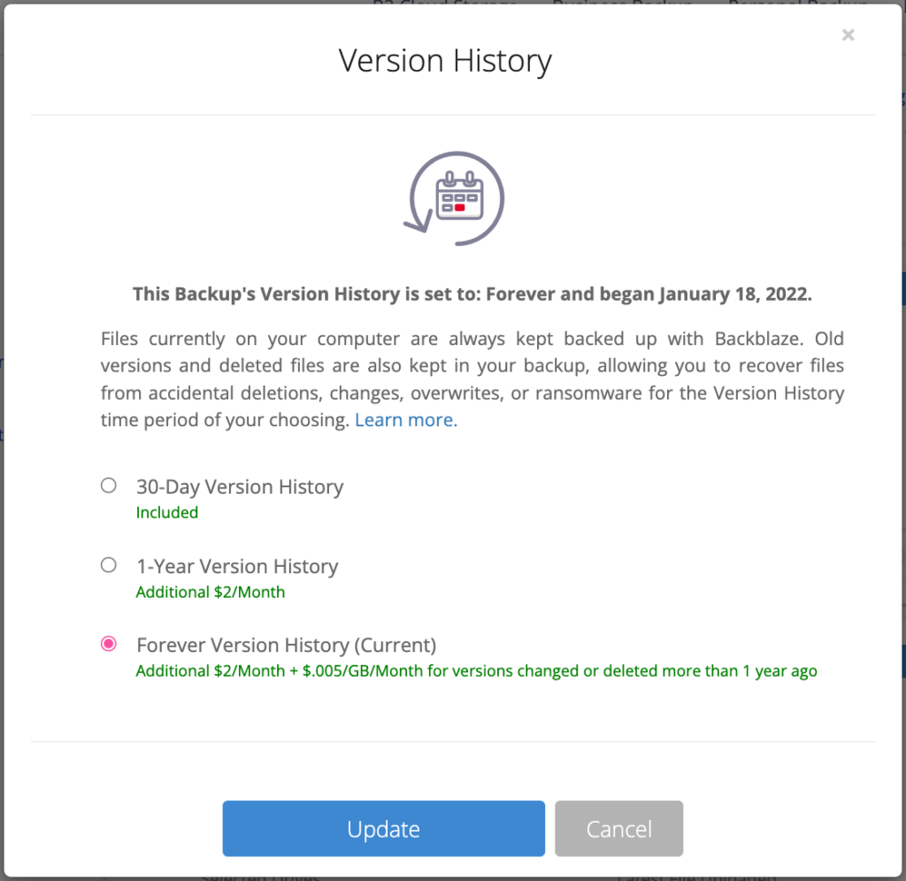
When you understand what retention is and what a version is, it’s easy to understand Extended Version History. It’s a feature that allows you to set a retention timeframe that specifies how long all the older versions—the version history—of your files should be kept as part of your backup.
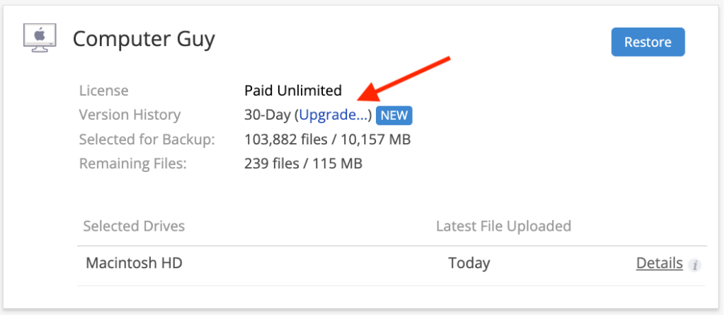
How Long Is Backblaze’s Retention?
The standard Backblaze Computer Backup service comes with 30 days of Version History for the files that are backed up. This means that you can go back in time (using our roll back time feature) and access older versions of files for 30 days from the date they were last changed or deleted. After that 30-day mark, the version of the file that’s 30 days old will leave your backup, but any newer files will remain.
Note: If you last changed or added a file more than 30 days ago, but have not made any changes to it, it will remain in your backup as long as it remains on your computer (or is unchanged). If it gets removed or changed, that’s when the 30-day retention period starts.
What Does Extended Version History Do?
With Extended Version History, you can increase that 30-day period to one year or even forever. This essentially increases the duration for which you can roll back time when going to access your data.
A Very Simple Example (With Babies!)
As a new uncle, I have babies on the brain. Let’s say that a baby was born on July 1st and our family creates a spreadsheet to chart the growth of the baby. Every single day, we add a row to the spreadsheet to add in the baby’s weight, height, and maybe a cute note. The previous rows don’t get deleted, and so the spreadsheet grows by one row every single day.
On July 30th, our spreadsheet will have 30 rows (one per day). If that spreadsheet was being backed up by Backblaze, I could go back in time to July 1st and get a copy of that spreadsheet from the very first day, with just a single row of baby information. However, if I tried to do that on July 31, that original version would be gone, but I could go back and get a copy from July 2nd, the version with the first two rows of baby data. If I tried to go back on, say, August 30th, I could get a copy from August 1, which would have all of July’s rows of baby data.
To illustrate the point, here’s me as a Soviet baby.
With Extended Version History, using that same example, I have more time (a year or forever) to go back and retrieve that original copy of the spreadsheet created on July 1 with just the first row.
Why would you want the spreadsheet with just one row? Who knows, it’s an example!
Why Extended Version History? Because Mistakes Happen!
Our Backup Awareness Month survey found that 67% of respondents have reported accidentally deleting a file. 44% reported losing data, or access to data, because a shared or synced drive or folder was deleted. Having Extended Version History turned on for your Backblaze backup helps avoid data loss because of accidental deletions.
You may not always realize right away (or within 30 days) that you deleted a file accidentally. Or you may not regularly check that shared drive until it’s too late and your older versions are gone. With Extended Version History, you can go back in time up to a year later or forever later and get those files back.
How to Get Extended Version History?
I encourage everyone I know to enable Extended Version History as soon as they install Backblaze on their computer.
Step 1: Click “Upgrade.”
Step 2: Select how long you want to keep files—one year or forever.
One thing to keep in mind is that simply turning on Extended Version History won’t automatically extend the “life” of your files retroactively. For example, if you open your account on July 1 and enable Extended Version History on July 28, only the versions from July 28 onward will have Extended Version History, not the versions created between July 1 and July 28. Once enabled, any new or changed files will have their retention rate increased, which is why doing so when you first install Backblaze is the best policy.
Consider Extended Version History as getting additional “mistake insurance” for your data. If something happens, or you lose access to shared files and that goes unnoticed, we’ll have your back!
The JavaScript community downloads over 5 billion packages from npm a day, and we at GitHub recognize how important it is that developers can do so with confidence. As stewards of the npm registry, it’s important that we continue to invest in improvements that increase developer trust and the overall security of the registry itself.
Today, we are announcing the general availability of an enhanced 2FA experience on npm, as well as sharing additional investments we’ve made to the verification process of accounts and packages.
The following improvements to npm are available today, including:
A streamlined login and publishing experience with the npm CLI.
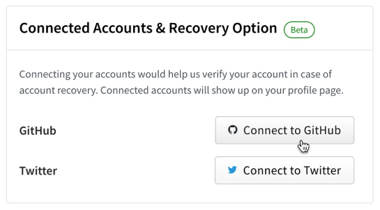
The ability to connect GitHub and Twitter accounts to npm.
All packages on npm have been re-signed and we’ve added a new npm CLI command to audit package integrity.
Streamlined login and publishing experience
Account security is significantly improved by adopting 2FA, but if the experience adds too much friction, we can’t expect customers to adopt it. We recently announced a variety of enhancements to the npm registry to make 2FA adoption easier for developers—in a public beta release. Early adopters of our new 2FA experience shared feedback around the process of logging in and publishing with the npm CLI, and we recognized there was room for improvement. Our initial design was created to be backwards compatible with npm 6 and other clients; in fact the Yarn project was able to backport support for our new experience to Yarn 1 in less than 10 lines of code!
We’ve been hard at work making the CLI experience better than ever based on this feedback, and the improved login and publish experience is now available in npm 8.15.0 today. With the new experience, users will benefit from:
Login and publish authentication are managed in the browser.
Login can use an existing session only prompting for your second factor or email verification OTP to create a new session.
Publish now supports “remember me for 5 minutes” and allows for subsequent publishes from the same IP + access token to avoid the 2FA prompt for a 5-minute period. This is especially useful when publishing from a npm workspace.
It is currently opt-in with the --auth-type=web flag and will be the default experience in npm 9.
These improved experiences will make it easier for users to secure their accounts. A secure account is the beginning of a secure ecosystem. Check out our documentation to learn more about 2FA in npm.
Connecting GitHub and Twitter Accounts to npm
Developers have been able to include their GitHub and Twitter handles on their npm profiles for almost as long as npm accounts have been available. This data has been helpful to connect the identity of an account on npm to an identity on other platforms; however this data has historically been a free-form text field that wasn’t validated or verified.
That’s why today we are launching the ability to link your npm account to your GitHub and Twitter accounts. Linking of these accounts is performed via official integrations with both GitHub and Twitter and ensures that verified account data are included on npm profiles moving forward. We will no longer be showing the previously unverified GitHub or Twitter data on public user profiles, making it possible for developers to audit identities and trust that an account is who they say they are.
Having a verified link between your identities across platforms significantly improves our ability to do account recovery. This new verified data lays the foundation for automating identity verification as part of account recovery. Over time, we will deprecate this legacy data, but we will continue to honor it for now to ensure that customers do not get locked out of their accounts.
You can verify your packages locally with npm audit signatures
Until today npm users have had to rely on a multi-step process to validate the signature of npm packages. This PGP based process was both complex and required users to have knowledge on cryptographic tools which provided a poor developer experience. Developers relying on this existing process should soon start using the new “audit signatures” command. The PGP keys are set to expire early next year with more details to follow.
Recently, we began work to re-sign all npm packages with new signatures relying on the secure ECDSA algorithm and using an HSM for key management, and you can now rely on this signature to verify the integrity of the packages you install from npm.
We have introduced a new audit signatures command in npm CLI version 8.13.0 and above.
Example of a successful audit signature verification
The below sample GitHub Actions workflow with audit signature in action.
Our primary goal continues to be protecting the npm registry, and our next major milestone will be enforcing 2FA for all high-impact accounts, those that manage packages with more than 1 million weekly downloads or 500 dependents, tripling the number of accounts we will require to adopt a second factor. Prior to this enforcement we will be making even more improvements to our account recovery process, including introducing additional forms of identity verification and automating as much of the process as possible.
Learn more about these features by visiting our documentation:
Кметът на Царево – Георги Лапчев /многомандатник ГЕРБ-ераст/ щял да обжалва заповедта за еко-защитата на залива Корал, става ясно от репортаж на БНР. Най-същественият мотив за обжалването на заповедта посочва…
AWS Single Sign-On (AWS SSO) is now AWS IAM Identity Center. Amazon Web Services (AWS) is changing the name to highlight the service’s foundation in AWS Identity and Access Management (IAM), to better reflect its full set of capabilities, and to reinforce its recommended role as the central place to manage access across AWS accounts and applications. Although the technical capabilities of the service haven’t changed with this announcement, we want to take the opportunity to walk through some of the important features that drive our recommendation to consider IAM Identity Center your front door into AWS.
If you’ve worked with AWS accounts, chances are that you’ve worked with IAM. This is the service that handles authentication and authorization requests for anyone who wants to do anything in AWS. It’s a powerful engine, processing half a billion API calls per second globally, and it has underpinned and secured the growth of AWS customers since 2011. IAM provides authentication on a granular basis—by resource, within each AWS account. Although this gives you unsurpassed ability to tailor permissions, it also requires that you establish permissions on an account-by-account basis for credentials (IAM users) that are also defined on an account-by-account basis.
As AWS customers increasingly adopted a multi-account strategy for their environments, in December 2017 we launched AWS Single Sign-On (AWS SSO)—a service built on top of IAM to simplify access management across AWS accounts. In the years since, customer adoption of multi-account AWS environments continued to increase the need for centralized access control and distributed access management. AWS SSO evolved accordingly, adding integrations with new identity providers, AWS services, and applications; features for the consistent management of permissions at scale; multiple compliance certifications; and availability in most AWS Regions. The variety of use cases supported by AWS SSO, now known as AWS IAM Identity Center, makes it our recommended way to manage AWS access for workforce users.
IAM Identity Center, just like AWS SSO before it, is offered at no extra charge. You can follow along with our walkthrough in your own console by choosing Getting started on the console main page. If you don’t have the service enabled, you will be prompted to choose Enable IAM Identity Center, as shown in Figure 1.
Figure 1: IAM Identity Center Getting Started page
Freedom to choose your identity source
Once you’re in the IAM Identity Center console, you can choose your preferred identity source for use across AWS, as shown in Figure 2. If you already have a workforce directory, you can continue to use it by connecting, or federating, it. You can connect to the major cloud identity providers, including Okta, Ping Identity, Azure AD, JumpCloud, CyberArk, and OneLogin, as well as Microsoft Active Directory Domain Services. If you don’t have or don’t want to use a workforce directory, you have the option to create users in Identity Center. Whichever source you decide to use, you connect or create it in one place for use in multiple accounts and AWS or SAML 2.0 applications.
Figure 2 Choosing and connecting your identity source
Management of fine-grained permissions at scale
As noted before, IAM Identity Center builds on the per-account capabilities of IAM. The difference is that in IAM Identity Center, you can define and assign access across multiple AWS accounts. For example, permission sets create IAM roles and apply IAM policies in multiple AWS accounts, helping to scale the access of your users securely and consistently.
You can use predefined permission sets based on AWS managed policies, or custom permission sets, where you can still start with AWS managed policies but then tailor them to your needs.
Recently, we added the ability to use IAM customer managed policies (CMPs) and permissions boundary policies as part of Identity Center permission sets, as shown in Figure 3. This helps you improve your security posture by creating larger and finer-grained policies for least privilege access and by tailoring them to reference the resources of the account to which they are applied. By using CMPs, you can maintain the consistency of your policies, because CMP changes apply automatically to the permission sets and roles that use the CMP. You can govern your CMPs and permissions boundaries centrally, and auditors can find, monitor, and review them in one place. If you already have existing CMPs for roles you manage in IAM, you can reuse them without the need to create, review, and approve new inline policies.
Figure 3: Specify permission sets in IAM Identity Center
By default, users and permission sets in IAM Identity Center are administered by the management account in an organization in AWS Organizations. This management account has the power and authority to manage member accounts in the organization as well. Because of the power of this account, it is important to exercise least privilege and tightly control access to it. If you are managing a complex organization supporting multiple operations or business units, IAM Identity Center allows you to delegate a member account that can administer user permissions, reducing the need to access the AWS Organizations management account for daily administrative work.
One place for application assignments
If your workforce uses Identity Center enabled applications, such as Amazon Managed Grafana, Amazon SageMaker Studio, or AWS Systems Manager Change Manager, you can assign access to them centrally, through IAM Identity Center, and your users can have a single sign-on experience.
If you do not have a separate cloud identity provider, you have the option to use IAM Identity Center as a single place to manage user assignments to SAML 2.0-based cloud applications, such as top-tier customer relationship management (CRM) applications, document collaboration tools, and productivity suites. Figure 4 shows this option.
Figure 4: Assign users to applications in IAM Identity Center
Conclusion
IAM Identity Center (the successor to AWS Single Sign-On) is where you centrally create or connect your workforce users once, and manage their access to multiple AWS accounts and applications. It’s our recommended front door into AWS, because it gives you the freedom to choose your preferred identity source for use across AWS, helps you strengthen your security posture with consistent permissions across AWS accounts and applications, and provides a convenient experience for your users. Its new name highlights the service’s foundation in IAM, while also reflecting its expanded capabilities and recommended role.
With Amazon GuardDuty, you can monitor your AWS accounts and workloads to detect malicious activity. Today, we are adding to GuardDuty the capability to detect malware. Malware is malicious software that is used to compromise workloads, repurpose resources, or gain unauthorized access to data. When you have GuardDuty Malware Protection enabled, a malware scan is initiated when GuardDuty detects that one of your EC2 instances or container workloads running on EC2 is doing something suspicious. For example, a malware scan is triggered when an EC2 instance is communicating with a command-and-control server that is known to be malicious or is performing denial of service (DoS) or brute-force attacks against other EC2 instances.
GuardDuty supports many file system types and scans file formats known to be used to spread or contain malware, including Windows and Linux executables, PDF files, archives, binaries, scripts, installers, email databases, and plain emails.
When potential malware is identified, actionable security findings are generated with information such as the threat and file name, the file path, the EC2 instance ID, resource tags and, in the case of containers, the container ID and the container image used. GuardDuty supports container workloads running on EC2, including customer-managed Kubernetes clusters or individual Docker containers. If the container is managed by Amazon Elastic Kubernetes Service (EKS) or Amazon Elastic Container Service (Amazon ECS), the findings also include the cluster name and the task or pod ID so application and security teams can quickly find the affected container resources.
As with all other GuardDuty findings, malware detections are sent to the GuardDuty console, pushed through Amazon EventBridge, routed to AWS Security Hub, and made available in Amazon Detective for incident investigation.
How GuardDuty Malware Protection Works When you enable malware protection, you set up an AWS Identity and Access Management (IAM)service-linked role that grants GuardDuty permissions to perform malware scans. When a malware scan is initiated for an EC2 instance, GuardDuty Malware Protection uses those permissions to take a snapshot of the attached Amazon Elastic Block Store (EBS) volumes that are less than 1 TB in size and then restore the EBS volumes in an AWS service account in the same AWS Region to scan them for malware. You can use tagging to include or exclude EC2 instances from those permissions and from scanning. In this way, you don’t need to deploy security software or agents to monitor for malware, and scanning the volumes doesn’t impact running workloads. The EBS volumes in the service account and the snapshots in your account are deleted after the scan. Optionally, you can preserve the snapshots when malware is detected.
The service-linked role grants GuardDuty access to AWS Key Management Service (AWS KMS) keys used to encrypt EBS volumes. If the EBS volumes attached to a potentially compromised EC2 instance are encrypted with a customer-managed key, GuardDuty Malware Protection uses the same key to encrypt the replica EBS volumes as well. If the volumes are not encrypted, GuardDuty uses its own key to encrypt the replica EBS volumes and ensure privacy. Volumes encrypted with EBS-managed keys are not supported.
Security in cloud is a shared responsibility between you and AWS. As a guardrail, the service-linked role used by GuardDuty Malware Protection cannot perform any operation on your resources (such as EBS snapshots and volumes, EC2 instances, and KMS keys) if it has the GuardDutyExcluded tag. Once you mark your snapshots with GuardDutyExcluded set to true, the GuardDuty service won’t be able to access these snapshots. The GuardDutyExcluded tag supersedes any inclusion tag. Permissions also restrict how GuardDuty can modify your snapshot so that they cannot be made public while shared with the GuardDuty service account.
The EBS volumes created by GuardDuty are always encrypted. GuardDuty can use KMS keys only on EBS snapshots that have a GuardDuty scan ID tag. The scan ID tag is added by GuardDuty when snapshots are created after an EC2 finding. The KMS keys that are shared with GuardDuty service account cannot be invoked from any other context except the Amazon EBS service. Once the scan completes successfully, the KMS key grant is revoked and the volume replica in GuardDuty service account is deleted, making sure GuardDuty service cannot access your data after completing the scan operation.
Enabling Malware Protection for an AWS Account If you’re not using GuardDuty yet, Malware Protection is enabled by default when you activate GuardDuty for your account. Because I am already using GuardDuty, I need to enable Malware Protection from the console. If you’re using AWS Organizations, your delegated administrator accounts can enable this for existing member accounts and configure if new AWS accounts in the organization should be automatically enrolled.
In the GuardDuty console, I choose Malware Protection under Settings in the navigation pane. There, I choose Enable and then Enable Malware Protection.
Snapshots are automatically deleted after they are scanned. In General settings, I have the option to retain in my AWS account the snapshots where malware is detected and have them available for further analysis.
In Scan options, I can configure a list of inclusion tags, so that only EC2 instances with those tags are scanned, or exclusion tags, so that EC2 instances with tags in the list are skipped.
Testing Malware Protection GuardDuty Findings To generate several Amazon GuardDuty findings, including the new Malware Protection findings, I clone the Amazon GuardDuty Tester repo:
First, I create an AWS CloudFormation stack using the guardduty-tester.template file. When the stack is ready, I follow the instructions to configure my SSH client to log in to the tester instance through the bastion host. Then, I connect to the tester instance:
$ ssh tester
From the tester instance, I start the guardduty_tester.sh script to generate the findings:
$ ./guardduty_tester.sh

***********************************************************************
* Test #1 - Internal port scanning                                    *
* This simulates internal reconaissance by an internal actor or an   *
* external actor after an initial compromise. This is considered a    *
* low priority finding for GuardDuty because its not a clear indicator*
* of malicious intent on its own.                                     *
***********************************************************************


Starting Nmap 6.40 ( http://nmap.org ) at 2022-05-19 09:36 UTC
Nmap scan report for ip-172-16-0-20.us-west-2.compute.internal (172.16.0.20)
Host is up (0.00032s latency).
Not shown: 997 filtered ports
PORT     STATE  SERVICE
22/tcp   open   ssh
80/tcp   closed http
5050/tcp closed mmcc
MAC Address: 06:25:CB:F4:E0:51 (Unknown)

Nmap done: 1 IP address (1 host up) scanned in 4.96 seconds

-----------------------------------------------------------------------

***********************************************************************
* Test #2 - SSH Brute Force with Compromised Keys                     *
* This simulates an SSH brute force attack on an SSH port that we    *
* can access from this instance. It uses (phony) compromised keys in  *
* many subsequent attempts to see if one works. This is a common      *
* techique where the bad actors will harvest keys from the web in     *
* places like source code repositories where people accidentally leave*
* keys and credentials (This attempt will not actually succeed in     *
* obtaining access to the target linux instance in this subnet)       *
***********************************************************************

2022-05-19 09:36:29 START
2022-05-19 09:36:29 Crowbar v0.4.3-dev
2022-05-19 09:36:29 Trying 172.16.0.20:22
2022-05-19 09:36:33 STOP
2022-05-19 09:36:33 No results found...
2022-05-19 09:36:33 START
2022-05-19 09:36:33 Crowbar v0.4.3-dev
2022-05-19 09:36:33 Trying 172.16.0.20:22
2022-05-19 09:36:37 STOP
2022-05-19 09:36:37 No results found...
2022-05-19 09:36:37 START
2022-05-19 09:36:37 Crowbar v0.4.3-dev
2022-05-19 09:36:37 Trying 172.16.0.20:22
2022-05-19 09:36:41 STOP
2022-05-19 09:36:41 No results found...
2022-05-19 09:36:41 START
2022-05-19 09:36:41 Crowbar v0.4.3-dev
2022-05-19 09:36:41 Trying 172.16.0.20:22
2022-05-19 09:36:45 STOP
2022-05-19 09:36:45 No results found...
2022-05-19 09:36:45 START
2022-05-19 09:36:45 Crowbar v0.4.3-dev
2022-05-19 09:36:45 Trying 172.16.0.20:22
2022-05-19 09:36:48 STOP
2022-05-19 09:36:48 No results found...
2022-05-19 09:36:49 START
2022-05-19 09:36:49 Crowbar v0.4.3-dev
2022-05-19 09:36:49 Trying 172.16.0.20:22
2022-05-19 09:36:52 STOP
2022-05-19 09:36:52 No results found...
2022-05-19 09:36:52 START
2022-05-19 09:36:52 Crowbar v0.4.3-dev
2022-05-19 09:36:52 Trying 172.16.0.20:22
2022-05-19 09:36:56 STOP
2022-05-19 09:36:56 No results found...
2022-05-19 09:36:56 START
2022-05-19 09:36:56 Crowbar v0.4.3-dev
2022-05-19 09:36:56 Trying 172.16.0.20:22
2022-05-19 09:37:00 STOP
2022-05-19 09:37:00 No results found...
2022-05-19 09:37:00 START
2022-05-19 09:37:00 Crowbar v0.4.3-dev
2022-05-19 09:37:00 Trying 172.16.0.20:22
2022-05-19 09:37:04 STOP
2022-05-19 09:37:04 No results found...
2022-05-19 09:37:04 START
2022-05-19 09:37:04 Crowbar v0.4.3-dev
2022-05-19 09:37:04 Trying 172.16.0.20:22
2022-05-19 09:37:08 STOP
2022-05-19 09:37:08 No results found...
2022-05-19 09:37:08 START
2022-05-19 09:37:08 Crowbar v0.4.3-dev
2022-05-19 09:37:08 Trying 172.16.0.20:22
2022-05-19 09:37:12 STOP
2022-05-19 09:37:12 No results found...
2022-05-19 09:37:12 START
2022-05-19 09:37:12 Crowbar v0.4.3-dev
2022-05-19 09:37:12 Trying 172.16.0.20:22
2022-05-19 09:37:16 STOP
2022-05-19 09:37:16 No results found...
2022-05-19 09:37:16 START
2022-05-19 09:37:16 Crowbar v0.4.3-dev
2022-05-19 09:37:16 Trying 172.16.0.20:22
2022-05-19 09:37:20 STOP
2022-05-19 09:37:20 No results found...
2022-05-19 09:37:20 START
2022-05-19 09:37:20 Crowbar v0.4.3-dev
2022-05-19 09:37:20 Trying 172.16.0.20:22
2022-05-19 09:37:23 STOP
2022-05-19 09:37:23 No results found...
2022-05-19 09:37:23 START
2022-05-19 09:37:23 Crowbar v0.4.3-dev
2022-05-19 09:37:23 Trying 172.16.0.20:22
2022-05-19 09:37:27 STOP
2022-05-19 09:37:27 No results found...
2022-05-19 09:37:27 START
2022-05-19 09:37:27 Crowbar v0.4.3-dev
2022-05-19 09:37:27 Trying 172.16.0.20:22
2022-05-19 09:37:31 STOP
2022-05-19 09:37:31 No results found...
2022-05-19 09:37:31 START
2022-05-19 09:37:31 Crowbar v0.4.3-dev
2022-05-19 09:37:31 Trying 172.16.0.20:22
2022-05-19 09:37:34 STOP
2022-05-19 09:37:34 No results found...
2022-05-19 09:37:35 START
2022-05-19 09:37:35 Crowbar v0.4.3-dev
2022-05-19 09:37:35 Trying 172.16.0.20:22
2022-05-19 09:37:38 STOP
2022-05-19 09:37:38 No results found...
2022-05-19 09:37:38 START
2022-05-19 09:37:38 Crowbar v0.4.3-dev
2022-05-19 09:37:38 Trying 172.16.0.20:22
2022-05-19 09:37:42 STOP
2022-05-19 09:37:42 No results found...
2022-05-19 09:37:42 START
2022-05-19 09:37:42 Crowbar v0.4.3-dev
2022-05-19 09:37:42 Trying 172.16.0.20:22
2022-05-19 09:37:46 STOP
2022-05-19 09:37:46 No results found...

-----------------------------------------------------------------------

***********************************************************************
* Test #3 - RDP Brute Force with Password List                        *
* This simulates an RDP brute force attack on the internal RDP port  *
* of the windows server that we installed in the environment.  It uses*
* a list of common passwords that can be found on the web. This test  *
* will trigger a detection, but will fail to get into the target      *
* windows instance.                                                   *
***********************************************************************

Sending 250 password attempts at the windows server...
Hydra v9.4-dev (c) 2022 by van Hauser/THC & David Maciejak - Please do not use in military or secret service organizations, or for illegal purposes (this is non-binding, these *** ignore laws and ethics anyway).

Hydra (https://github.com/vanhauser-thc/thc-hydra) starting at 2022-05-19 09:37:46
[WARNING] rdp servers often don't like many connections, use -t 1 or -t 4 to reduce the number of parallel connections and -W 1 or -W 3 to wait between connection to allow the server to recover
[INFO] Reduced number of tasks to 4 (rdp does not like many parallel connections)
[WARNING] the rdp module is experimental. Please test, report - and if possible, fix.
[DATA] max 4 tasks per 1 server, overall 4 tasks, 1792 login tries (l:7/p:256), ~448 tries per task
[DATA] attacking rdp://172.16.0.24:3389/
[STATUS] 1099.00 tries/min, 1099 tries in 00:01h, 693 to do in 00:01h, 4 active
1 of 1 target completed, 0 valid password found
Hydra (https://github.com/vanhauser-thc/thc-hydra) finished at 2022-05-19 09:39:23

-----------------------------------------------------------------------

***********************************************************************
* Test #4 - CryptoCurrency Mining Activity                            *
* This simulates interaction with a cryptocurrency mining pool which *
* can be an indication of an instance compromise. In this case, we are*
* only interacting with the URL of the pool, but not downloading      *
* any files. This will trigger a threat intel based detection.        *
***********************************************************************

Calling bitcoin wallets to download mining toolkits

-----------------------------------------------------------------------

***********************************************************************
* Test #5 - DNS Exfiltration                                          *
* A common exfiltration technique is to tunnel data out over DNS      *
* to a fake domain.  Its an effective technique because most hosts    *
* have outbound DNS ports open.  This test wont exfiltrate any data,  *
* but it will generate enough unusual DNS activity to trigger the     *
* detection.                                                          *
***********************************************************************

Calling large numbers of large domains to simulate tunneling via DNS

***********************************************************************
* Test #6 - Fake domain to prove that GuardDuty is working            *
* This is a permanent fake domain that customers can use to prove that*
* GuardDuty is working.  Calling this domain will always generate the *
* Backdoor:EC2/C&CActivity.B!DNS finding type                         *
***********************************************************************

Calling a well known fake domain that is used to generate a known finding

; <<>> DiG 9.11.4-P2-RedHat-9.11.4-26.P2.amzn2.5.2 <<>> GuardDutyC2ActivityB.com any
;; global options: +cmd
;; Got answer:
;; ->>HEADER<<- opcode: QUERY, status: NOERROR, id: 11495
;; flags: qr rd ra; QUERY: 1, ANSWER: 8, AUTHORITY: 0, ADDITIONAL: 1

;; OPT PSEUDOSECTION:
; EDNS: version: 0, flags:; udp: 4096
;; QUESTION SECTION:
;GuardDutyC2ActivityB.com.	IN	ANY

;; ANSWER SECTION:
GuardDutyC2ActivityB.com. 6943	IN	SOA	ns1.markmonitor.com. hostmaster.markmonitor.com. 2018091906 86400 3600 2592000 172800
GuardDutyC2ActivityB.com. 6943	IN	NS	ns3.markmonitor.com.
GuardDutyC2ActivityB.com. 6943	IN	NS	ns5.markmonitor.com.
GuardDutyC2ActivityB.com. 6943	IN	NS	ns7.markmonitor.com.
GuardDutyC2ActivityB.com. 6943	IN	NS	ns2.markmonitor.com.
GuardDutyC2ActivityB.com. 6943	IN	NS	ns4.markmonitor.com.
GuardDutyC2ActivityB.com. 6943	IN	NS	ns6.markmonitor.com.
GuardDutyC2ActivityB.com. 6943	IN	NS	ns1.markmonitor.com.

;; Query time: 27 msec
;; SERVER: 172.16.0.2#53(172.16.0.2)
;; WHEN: Thu May 19 09:39:23 UTC 2022
;; MSG SIZE  rcvd: 238


*****************************************************************************************************
Expected GuardDuty Findings

Test 1: Internal Port Scanning
Expected Finding: EC2 Instance  i-011e73af27562827b  is performing outbound port scans against remote host. 172.16.0.20
Finding Type: Recon:EC2/Portscan

Test 2: SSH Brute Force with Compromised Keys
Expecting two findings - one for the outbound and one for the inbound detection
Outbound:  i-011e73af27562827b  is performing SSH brute force attacks against  172.16.0.20
Inbound:  172.16.0.25  is performing SSH brute force attacks against  i-0bada13e0aa12d383
Finding Type: UnauthorizedAccess:EC2/SSHBruteForce

Test 3: RDP Brute Force with Password List
Expecting two findings - one for the outbound and one for the inbound detection
Outbound:  i-011e73af27562827b  is performing RDP brute force attacks against  172.16.0.24
Inbound:  172.16.0.25  is performing RDP brute force attacks against  i-0191573dec3b66924
Finding Type : UnauthorizedAccess:EC2/RDPBruteForce

Test 4: Cryptocurrency Activity
Expected Finding: EC2 Instance  i-011e73af27562827b  is querying a domain name that is associated with bitcoin activity
Finding Type : CryptoCurrency:EC2/BitcoinTool.B!DNS

Test 5: DNS Exfiltration
Expected Finding: EC2 instance  i-011e73af27562827b  is attempting to query domain names that resemble exfiltrated data
Finding Type : Trojan:EC2/DNSDataExfiltration

Test 6: C&C Activity
Expected Finding: EC2 instance  i-011e73af27562827b  is querying a domain name associated with a known Command & Control server.
Finding Type : Backdoor:EC2/C&CActivity.B!DNS
After a few minutes, the findings appear in the GuardDuty console. At the top, I see the malicious files found by the new Malware Protection capability. One of the findings is related to an EC2 instance, the other to an ECS cluster.
First, I select the finding related to the EC2 instance. In the panel, I see the information on the instance and the malicious file, such as the file name and path. In the Malware scan details section, the Trigger finding ID points to the original GuardDuty finding that triggered the malware scan. In my case, the original finding was that this EC2 instance was performing RDP brute force attacks against another EC2 instance.
Here, I choose Investigate with Detective and, directly from the GuardDuty console, I go to the Detective console to visualize AWS CloudTrail and Amazon Virtual Private Cloud (Amazon VPC) flow data for the EC2 instance, the AWS account, and the IP address affected by the finding. Using Detective, I can analyze, investigate, and identify the root cause of suspicious activities found by GuardDuty.
When I select the finding related to the ECS cluster, I have more information on the resource affected, such as the details of the ECS cluster, the task, the containers, and the container images.
Using the GuardDuty tester scripts makes it easier to test the overall integration of GuardDuty with other security frameworks you use so that you can be ready when a real threat is detected.
Comparing GuardDuty Malware Protection with Amazon Inspector At this point, you might ask yourself how GuardDuty Malware Protection relates to Amazon Inspector, a service that scans AWS workloads for software vulnerabilities and unintended network exposure. The two services complement each other and offer different layers of protection:
Amazon Inspector offers proactive protection by identifying and remediating known software and application vulnerabilities that serve as an entry point for attackers to compromise resources and install malware.
GuardDuty Malware Protection detects malware that is found to be present on actively running workloads. At that point, the system has already been compromised, but GuardDuty can limit the time of an infection and take action before a system compromise results in a business-impacting event.
Availability and Pricing Amazon GuardDuty Malware Protection is available today in all AWS Regions where GuardDuty is available, excluding the AWS China (Beijing), AWS China (Ningxia), AWS GovCloud (US-East), and AWS GovCloud (US-West) Regions.
At launch, GuardDuty Malware Protection is integrated with these partner offerings:
With GuardDuty, you don’t need to deploy security software or agents to monitor for malware. You only pay for the amount of GB scanned in the file systems (not for the size of the EBS volumes) and for the EBS snapshots during the time they are kept in your account. All EBS snapshots created by GuardDuty are automatically deleted after they are scanned unless you enable snapshot retention when malware is found. For more information, see GuardDuty pricing and EBS pricing. Note that GuardDuty only scans EBS volumes less than 1 TB in size. To help you control costs and avoid repeating alarms, the same volume is not scanned more often than once every 24 hours.
In March 2020, we introduced Amazon Detective, a fully managed service that makes it easy to analyze, investigate, and quickly identify the root cause of potential security issues or suspicious activities.
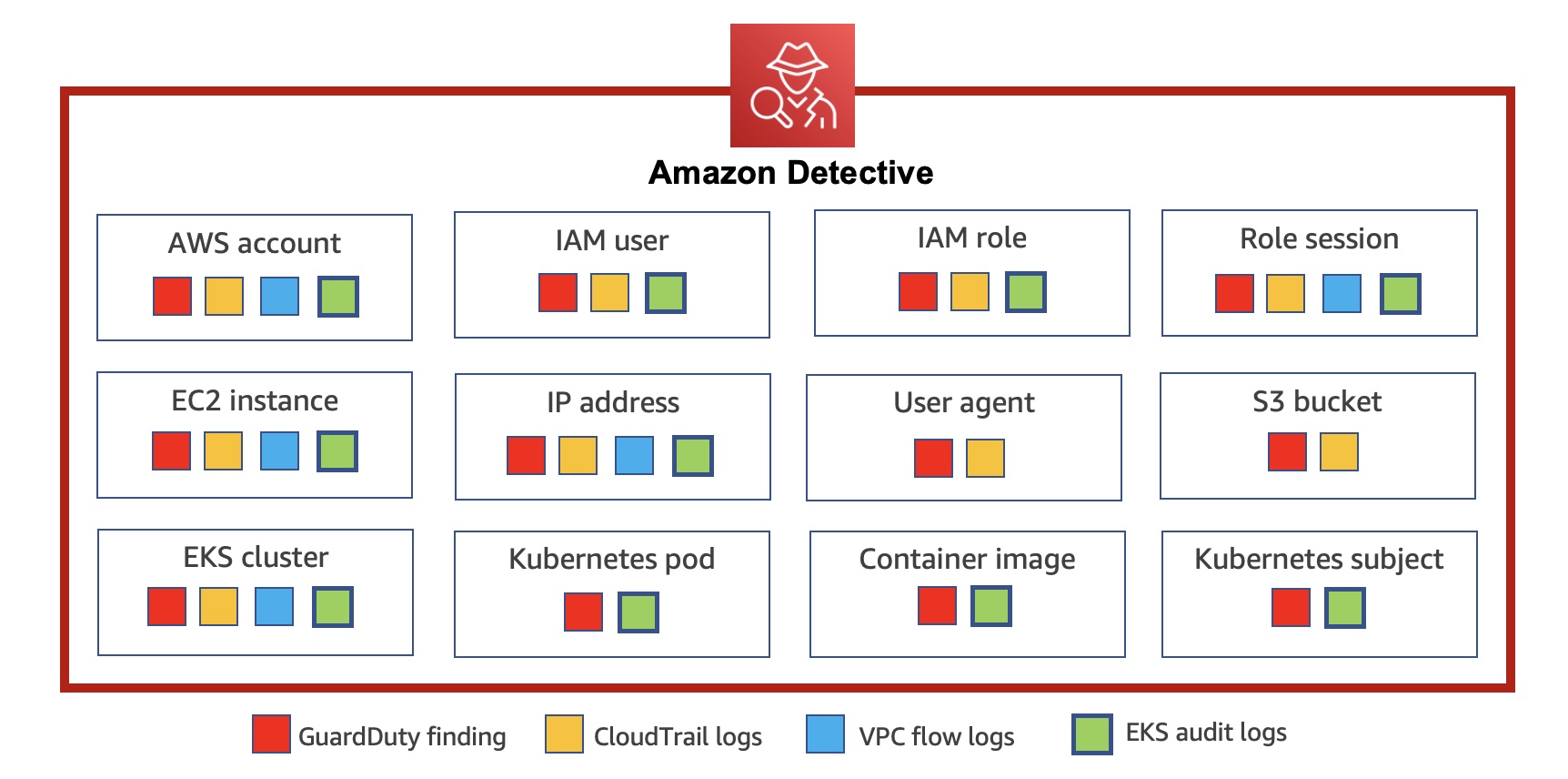
Customers are rapidly moving to containers to deploy Kubernetes workloads with Amazon Elastic Kubernetes Service (Amazon EKS). Its highly programmatic nature allows thousands of individual container deployments and millions of configuration changes to occur in seconds. To effectively secure EKS workloads, it is important to monitor container deployments and configurations that are captured in the form of EKS audit logs and to correlate activities to user activity and network traffic happening across AWS accounts.
Today we announce new capabilities in Amazon Detective to expand security investigation coverage for Kubernetes workloads running on Amazon EKS. When you enable this new feature, Amazon Detective automatically starts ingesting EKS audit logs to capture chronological API activity from users, applications, and the control plane in Amazon EKS for clusters, pods, container images, and Kubernetes subjects (Kubernetes users and service accounts).
Detective automatically correlates user activity using CloudTrail, and network activity using Amazon VPC Flow logs, without the need for you to enable, store, or retain logs manually. The service gleans key security information from these logs and retains them in a security behavioral graph database that enables fast cross-referenced access to twelve months of activity. Detective provides a data analysis and visualization layer purpose-built to answer common security questions backed by a behavioral graph database that allows you to quickly investigate potential malicious behavior associated with your EKS workloads.
You can rapidly respond to security issues rather than focusing on log management, operational systems, or ongoing security tooling maintenance. Detective’s EKS capabilities come with a free 30-day trial for all customers that allows you to ensure that the capabilities meet your needs and to fully understand the cost for the service on an ongoing basis.
Getting Started with Security Investigations for EKS Audit Logs To get started, enable Amazon Detective with just a few clicks in the AWS Management Console. GuardDuty is a prerequisite of Amazon Detective. When you try to enable Detective, Detective checks whether GuardDuty has been enabled for your account. You must either enable GuardDuty or wait for 48 hours. This allows GuardDuty to assess the data volume that your account produces.
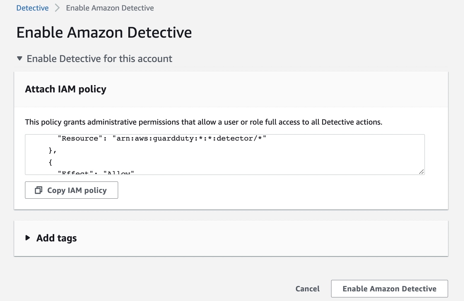
You can enable your account by attaching the AWS IAM policy or delegate it to an administrator of your organization. To learn more, refer to Setting up Detective in the AWS documentation.
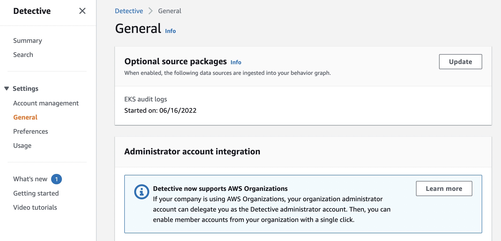
To enable EKS support in Detective as an existing customer, navigate to the Settings menu in the left panel and select General. Under Optional source packages, enable EKS audit logs.
If you are a new customer of Detective, the EKS protection feature will be enabled by default. If you do not want to trial EKS audit logs right away, you can disable this feature within the first week of enabling Detective and preserve the full 30-day free trial period to use in the future.
Once enabled, Detective will begin monitoring the Kubernetes audit logs that are generated by Amazon EKS, extracting and correlating information for security usage. You do not need to enable any log sources or make any configuration changes to your existing EKS clusters or future deployments.
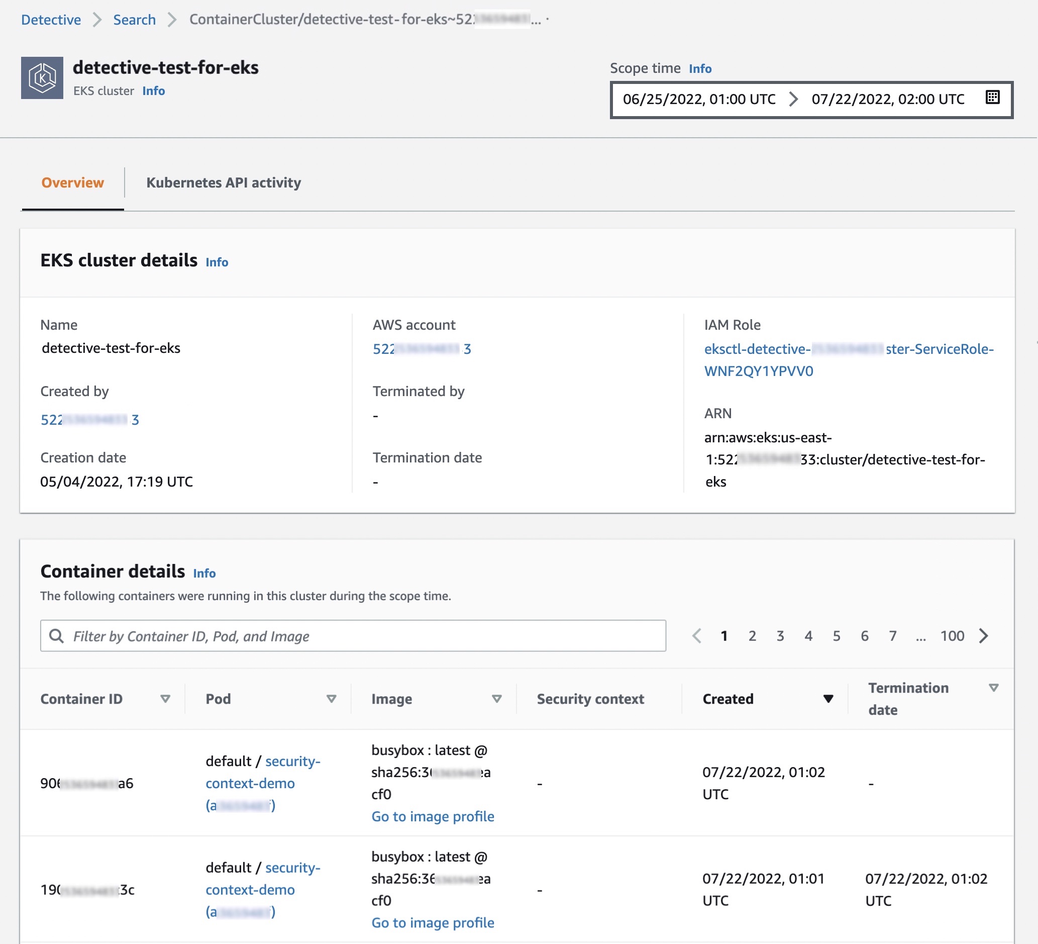
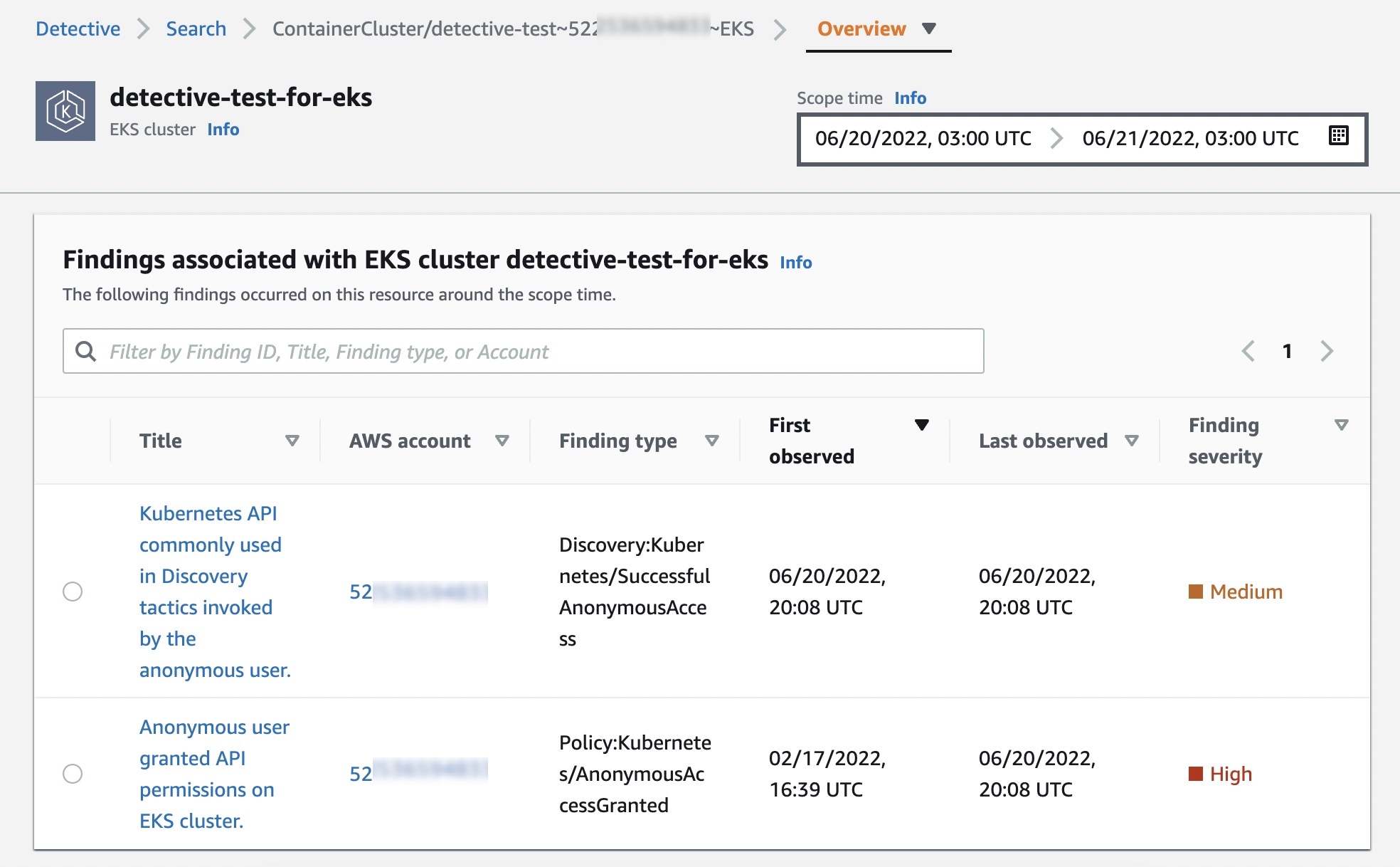
You can see recent monitoring results of your EKS clusters on the Summary page.
When you choose one of the EKS clusters, you will see the details of containers running in the cluster, Kubernetes API activities, and network activities that occurred on this resource around the scope time.
In the Overview tab, you also see details about all containers running in the cluster, including their pod, image and security context.
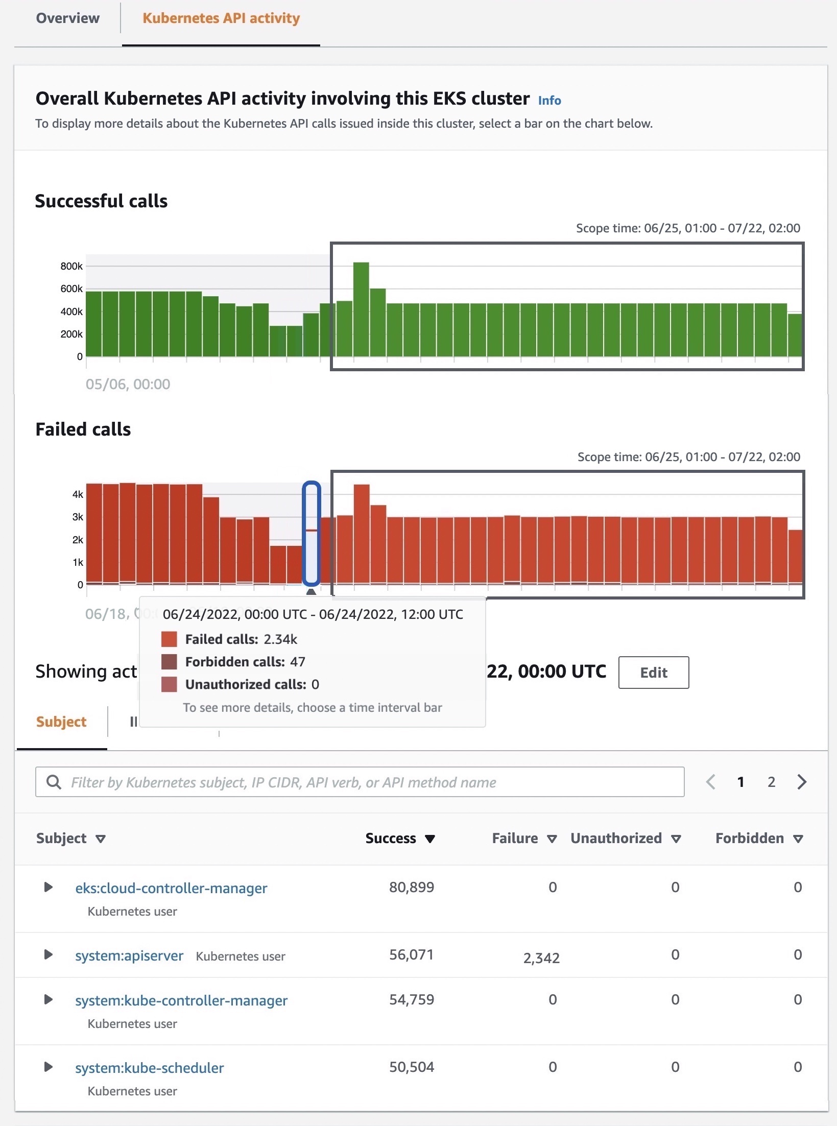
In the Kubernetes API activity tab, you can get an overview of the full API activities involving the EKS cluster. You can choose a time range to drill down based on specific API methods within the EKS cluster. When you select a specific time, you can see API subjects, IP addresses, and the number of API calls by the success, failure, unauthorized, or forbidden state.
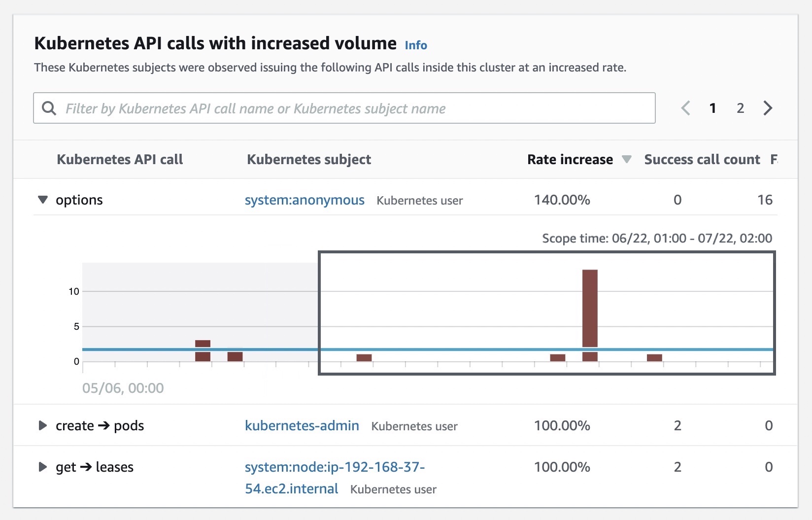
You can also see details of newly observed Kubernetes API calls inside this cluster for the first time and subjects with increased volume that happened inside the cluster.
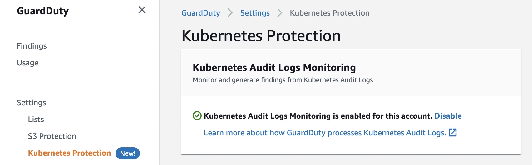
Enabling GuardDuty EKS Protection In January 2022, Amazon GuardDuty expanded coverage to EKS cluster activity to identify malicious or suspicious behavior that represents potential threats to container workloads.
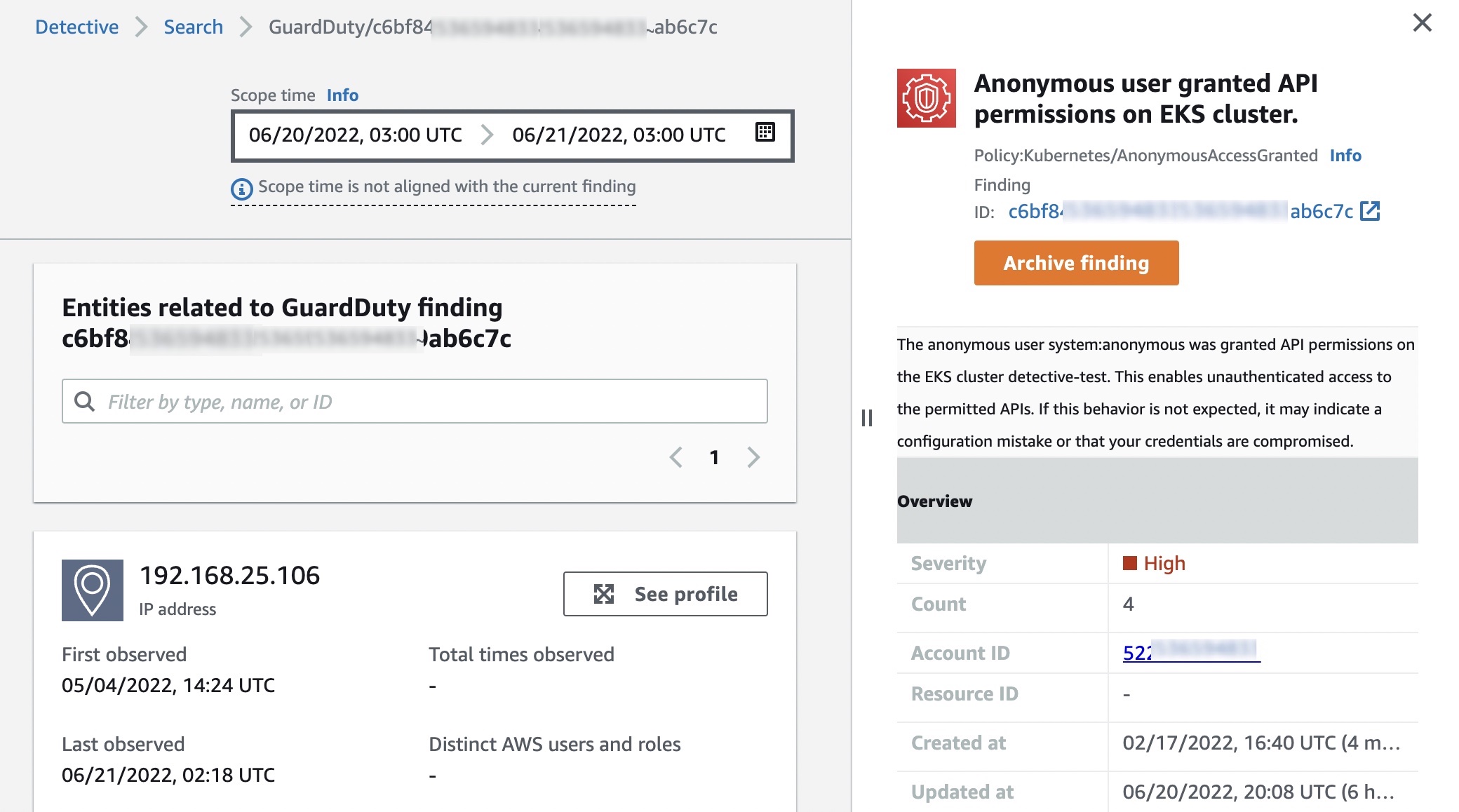
When the optional GuardDuty EKS Protection is enabled, GuardDuty will continuously monitor your EKS deployments and alert you to threats detected in your workloads. You can view and investigate these security findings in Detective.
With Detective for EKS enabled, you can quickly access information about the resources involved in the finding, such as their CloudTrail and Kubernetes API activity, and netflow information. This can aid in investigation and help you determine root cause, impact, and other related resources that may also be compromised.
Now Available You can now use Amazon Detective for EKS protection in all Regions where Amazon Detective is available. This feature is priced based on the volume of audit logs processed and analyzed by Detective.
Detective provides a free 30-day trial to all customers that enable EKS coverage, allowing customers to ensure that Detective’s capabilities meet security needs and to get an estimate of the service’s monthly cost before committing to paid usage. To learn more, see the Detective pricing page.
Security updates have been issued by Debian (spip), Mageia (libtiff and logrotate), Oracle (java-1.8.0-openjdk and java-11-openjdk), SUSE (gpg2, logrotate, and phpPgAdmin), and Ubuntu (python-bottle).
Over the years I’ve been lurking around the Linux kernel and have investigated the TCP code many times. But when recently we were working on Optimizing TCP for high WAN throughput while preserving low latency, I realized I have gaps in my knowledge about how Linux manages TCP receive buffers and windows. As I dug deeper I found the subject complex and certainly non-obvious.
In this blog post I’ll share my journey deep into the Linux networking stack, trying to understand the memory and window management of the receiving side of a TCP connection. Specifically, looking for answers to seemingly trivial questions:
How much data can be stored in the TCP receive buffer? (it’s not what you think)
How fast can it be filled? (it’s not what you think either!)
Our exploration focuses on the receiving side of the TCP connection. We’ll try to understand how to tune it for the best speed, without wasting precious memory.
A case of a rapid upload
To best illustrate the receive side buffer management we need pretty charts! But to grasp all the numbers, we need a bit of theory.
We’ll draw charts from a receive side of a TCP flow, running a pretty straightforward scenario:
The client opens a TCP connection.
The client does send(), and pushes as much data as possible.
The server doesn’t recv() any data. We expect all the data to stay and wait in the receive queue.
How much data can fit in the server’s receive buffer? It turns out it’s not exactly the same as the default read buffer size on Linux; we’ll get there.
Assuming infinite bandwidth, what is the minimal time – measured in RTT – for the client to fill the receive buffer?
First, there is the buffer budget limit. ss manpage calls it skmem_rb, in the kernel it’s named sk_rcvbuf. This value is most often controlled by the Linux autotune mechanism using the net.ipv4.tcp_rmem setting:
Alternatively it can be manually set with setsockopt(SO_RCVBUF) on a socket. Note that the kernel doubles the value given to this setsockopt. For example SO_RCVBUF=16384 will result in skmem_rb=32768. The max value allowed to this setsockopt is limited to meager 208KiB by default:
The aforementioned blog post discusses why manual buffer size management is problematic – relying on autotuning is generally preferable.
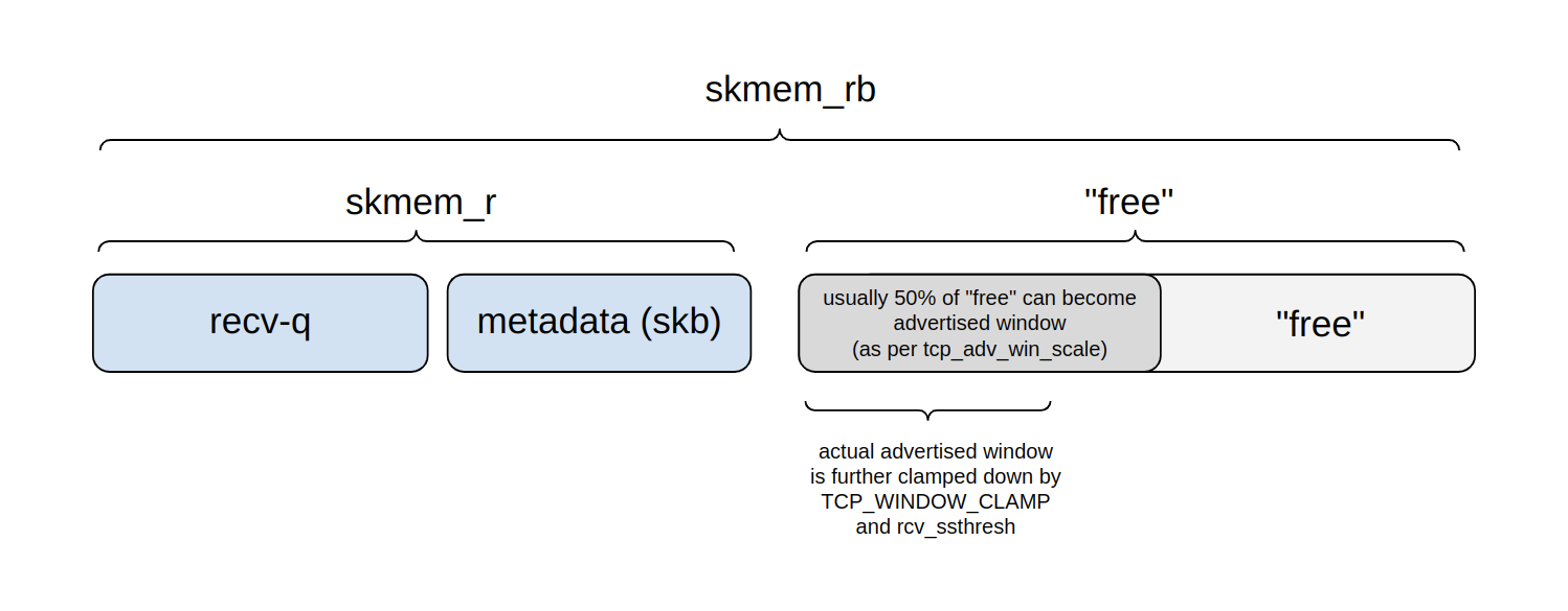
Here’s a diagram showing how skmem_rb budget is being divided:
In any given moment, we can think of the budget as being divided into four parts:
Recv-q: part of the buffer budget occupied by actual application bytes awaiting read().
Another part of is consumed by metadata handling – the cost of struct sk_buff and such.
Those two parts together are reported by ss as skmem_r – kernel name is sk_rmem_alloc.
What remains is “free”, that is: it’s not actively used yet.
However, a portion of this “free” region is an advertised window – it may become occupied with application data soon.
The remainder will be used for future metadata handling, or might be divided into the advertised window further in the future.
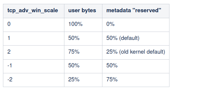
The upper limit for the window is configured by tcp_adv_win_scale setting. By default, the window is set to at most 50% of the “free” space. The value can be clamped further by the TCP_WINDOW_CLAMP option or an internal rcv_ssthresh variable.
How much data can a server receive?
Our first question was “How much data can a server receive?”. A naive reader might think it’s simple: if the server has a receive buffer set to say 64KiB, then the client will surely be able to deliver 64KiB of data!
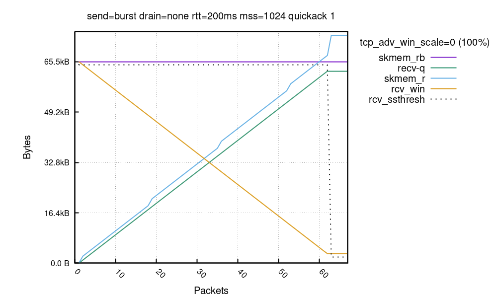
But this is totally not how it works. To illustrate this, allow me to temporarily set sysctl tcp_adv_win_scale=0. This is not a default and, as we’ll learn, it’s the wrong thing to do. With this setting the server will indeed set 100% of the receive buffer as an advertised window.
Here’s our setup:
The client tries to send as fast as possible.
Since we are interested in the receiving side, we can cheat a bit and speed up the sender arbitrarily. The client has transmission congestion control disabled: we set initcwnd=10000 as the route option.
The server has a fixed skmem_rb set at 64KiB.
The server has tcp_adv_win_scale=0.
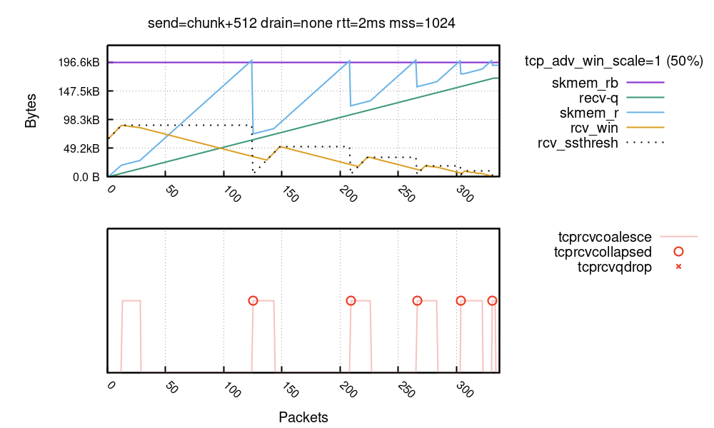
There are so many things here! Let’s try to digest it. First, the X axis is an ingress packet number (we saw about 65). The Y axis shows the buffer sizes as seen on the receive path for every packet.
First, the purple line is a buffer size limit in bytes – skmem_rb. In our experiment we called setsockopt(SO_RCVBUF)=32K and skmem_rb is double that value. Notice, by calling SO_RCVBUF we disabled the Linux autotune mechanism.
Green recv-q line is how many application bytes are available in the receive socket. This grows linearly with each received packet.
Then there is the blue skmem_r, the used data + metadata cost in the receive socket. It grows just like recv-q but a bit faster, since it accounts for the cost of the metadata kernel needs to deal with.
The orange rcv_win is an advertised window. We start with 64KiB (100% of skmem_rb) and go down as the data arrives.
Finally, the dotted line shows rcv_ssthresh, which is not important yet, we’ll get there.
Running over the budget is bad
It’s super important to notice that we finished with skmem_r higher than skmem_rb! This is rather unexpected, and undesired. The whole point of the skmem_rb memory budget is, well, not to exceed it. Here’s how ss shows it:
$ ss -m
Netid  State  Recv-Q  Send-Q  Local Address:Port  Peer Address:Port
tcp    ESTAB  62464   0       127.0.0.3:1234      127.0.0.2:1235
     skmem:(r73984,rb65536,...)
As you can see, skmem_rb is 65536 and skmem_r is 73984, which is 8448 bytes over! When this happens we have an even bigger issue on our hands. At around the 62nd packet we have an advertised window of 3072 bytes, but while packets are being sent, the receiver is unable to process them! This is easily verifiable by inspecting an nstat TcpExtTCPRcvQDrop counter:
In our run 13 packets were dropped. This variable counts a number of packets dropped due to either system-wide or per-socket memory pressure – we know we hit the latter. In our case, soon after the socket memory limit was crossed, new packets were prevented from being enqueued to the socket. This happened even though the TCP advertised window was still open.
This results in an interesting situation. The receiver’s window is open which might indicate it has resources to handle the data. But that’s not always the case, like in our example when it runs out of the memory budget.
The sender will think it hit a network congestion packet loss and will run the usual retry mechanisms including exponential backoff. This behavior can be looked at as desired or undesired, depending on how you look at it. On one hand no data will be lost, the sender can eventually deliver all the bytes reliably. On the other hand the exponential backoff logic might stall the sender for a long time, causing a noticeable delay.
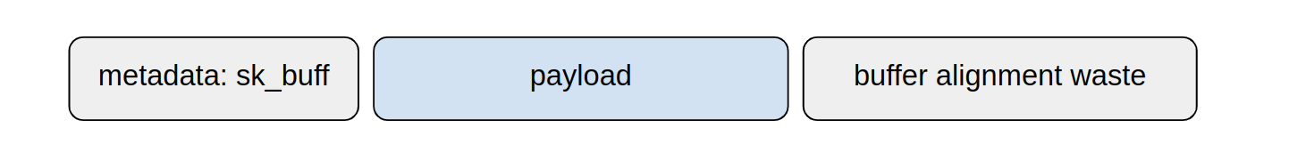
The root of the problem is straightforward – Linux kernel skmem_rb sets a memory budget for both the data and metadata which reside on the socket. In a pessimistic case each packet might incur a cost of a struct sk_buff + struct skb_shared_info, which on my system is 576 bytes, above the actual payload size, plus memory waste due to network card buffer alignment:
We now understand that Linux can’t just advertise 100% of the memory budget as an advertised window. Some budget must be reserved for metadata and such. The upper limit of window size is expressed as a fraction of the “free” socket budget. It is controlled by tcp_adv_win_scale, with the following values:
By default, Linux sets the advertised window at most at 50% of the remaining buffer space.
Even with 50% of space “reserved” for metadata, the kernel is very smart and tries hard to reduce the metadata memory footprint. It has two mechanisms for this:
TCP Coalesce – on the happy path, Linux is able to throw away struct sk_buff. It can do so, by just linking the data to the previously enqueued packet. You can think about it as if it was extending the last packet on the socket.
TCP Collapse – when the memory budget is hit, Linux runs “collapse” code. Collapse rewrites and defragments the receive buffer from many small skb’s into a few very long segments – therefore reducing the metadata cost.
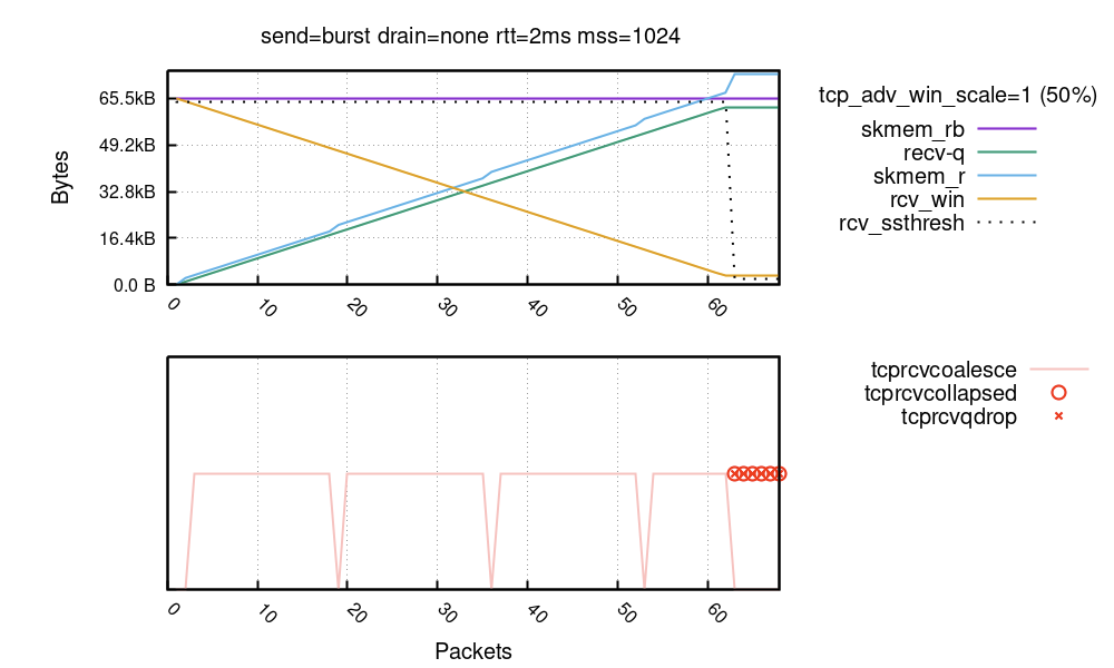
Here’s an extension to our previous chart showing these mechanisms in action:
TCP Coalesce is a very effective measure and works behind the scenes at all times. In the bottom chart, the packets where the coalesce was engaged are shown with a pink line. You can see – the skmem_r bumps (blue line) are clearly correlated with a lack of coalesce (pink line)! The nstat TcpExtTCPRcvCoalesce counter might be helpful in debugging coalesce issues.
The TCP Collapse is a bigger gun. Mike wrote about it extensively, and I wrote a blog post years ago, when the latency of TCP collapse hit us hard. In the chart above, the collapse is shown as a red circle. We clearly see it being engaged after the socket memory budget is reached – from packet number 63. The nstat TcpExtTCPRcvCollapsed counter is relevant here. This value growing is a bad sign and might indicate bad latency spikes – especially when dealing with larger buffers. Normally collapse is supposed to be run very sporadically. A prominent kernel developer describes this pessimistic situation:
This also means tcp advertises a too optimistic window for a given allocated rcvspace: When receiving frames, sk_rmem_alloc can hit sk_rcvbuf limit and we call tcp_collapse() too often, especially when application is slow to drain its receive queue […] This is a major latency source.
If the memory budget remains exhausted after the collapse, Linux will drop ingress packets. In our chart it’s marked as a red “X”. The nstat TcpExtTCPRcvQDrop counter shows the count of dropped packets.
rcv_ssthresh predicts the metadata cost
Perhaps counter-intuitively, the memory cost of a packet can be much larger than the amount of actual application data contained in it. It depends on number of things:
Network card: some network cards always allocate a full page (4096, or even 16KiB) per packet, no matter how small or large the payload.
Payload size: shorter packets, will have worse metadata to content ratio since struct skb will be comparably larger.
Whether XDP is being used.
L2 header size: things like ethernet, vlan tags, and tunneling can add up.
Cache line size: many kernel structs are cache line aligned. On systems with larger cache lines, they will use more memory (see P4 or S390X architectures).
The first two factors are the most important. Here’s a run when the sender was specially configured to make the metadata cost bad and the coalesce ineffective (the details of the setup are messy):
You can see the kernel hitting TCP collapse multiple times, which is totally undesired. Each time a collapse kernel is likely to rewrite the full receive buffer. This whole kernel machinery, from reserving some space for metadata with tcp_adv_win_scale, via using coalesce to reduce the memory cost of each packet, up to the rcv_ssthresh limit, exists to avoid this very case of hitting collapse too often.
* The scheme does not work when sender sends good segments opening
* window and then starts to feed us spaghetti. But it should work
* in common situations. Otherwise, we have to rely on queue collapsing.
Notice that the rcv_ssthresh line dropped down on the TCP collapse. This variable is an internal limit to the advertised window. By dropping it the kernel effectively says: hold on, I mispredicted the packet cost, next time I’m given an opportunity I’m going to open a smaller window. Kernel will advertise a smaller window and be more careful – all of this dance is done to avoid the collapse.
Normal run – continuously updated window
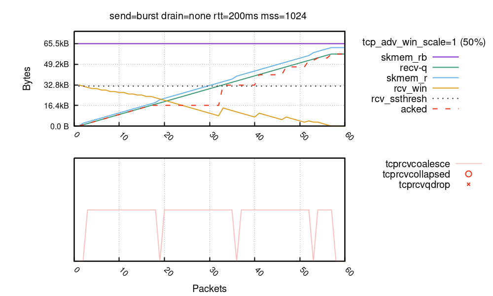
Finally, here’s a chart from a normal run of a connection. Here, we use the default tcp_adv_win_wcale=1 (50%):
Early in the connection you can see rcv_win being continuously updated with each received packet. This makes sense: while the rcv_ssthresh and tcp_adv_win_scale restrict the advertised window to never exceed 32KiB, the window is sliding nicely as long as there is enough space. At packet 18 the receiver stops updating the window and waits a bit. At packet 32 the receiver decides there still is some space and updates the window again, and so on. At the end of the flow the socket has 56KiB of data. This 56KiB of data was received over a sliding window reaching at most 32KiB .
The saw blade pattern of rcv_win is enabled by delayed ACK (aka QUICKACK). You can see the “acked” bytes in red dashed line. Since the ACK’s might be delayed, the receiver waits a bit before updating the window. If you want a smooth line, you can use quickack 1 per-route parameter, but this is not recommended since it will result in many small ACK packets flying over the wire.
In normal connection we expect the majority of packets to be coalesced and the collapse/drop code paths never to be hit.
Large receive windows – rcv_ssthresh
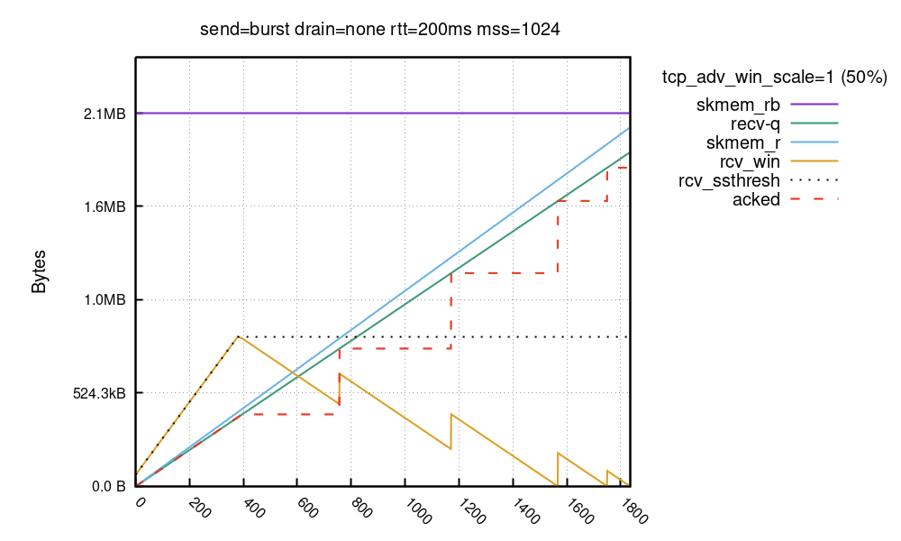
For large bandwidth transfers over big latency links – big BDP case – it’s beneficial to have a very wide advertised window. However, Linux takes a while to fully open large receive windows:
In this run, the skmem_rb is set to 2MiB. As opposed to previous runs, the buffer budget is large and the receive window doesn’t start with 50% of the skmem_rb! Instead it starts from 64KiB and grows linearly. It takes a while for Linux to ramp up the receive window to full size – ~800KiB in this case. The window is clamped by rcv_ssthresh. This variable starts at 64KiB and then grows at a rate of two full-MSS packets per each packet which has a “good” ratio of total size (truesize) to payload size.
Stack is conservative about RWIN increase, it wants to receive packets to have an idea of the skb->len/skb->truesize ratio to convert a memory budget to RWIN. Some drivers have to allocate 16K buffers (or even 32K buffers) just to hold one segment (of less than 1500 bytes of payload), while others are able to pack memory more efficiently.
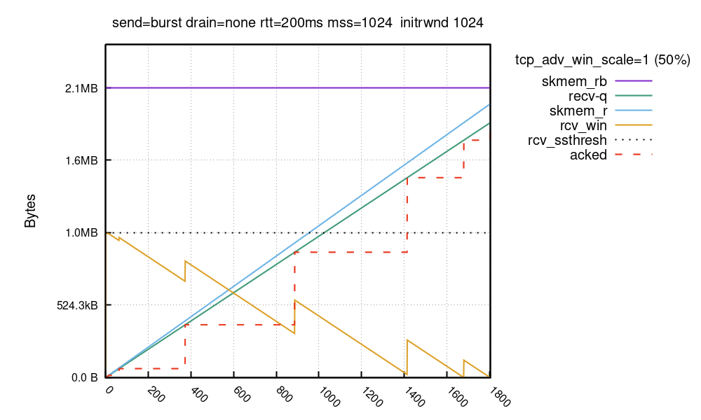
$ ip route change local 127.0.0.0/8 dev lo initrwnd 1000
With the patch and the route change deployed, this is how the buffers look:
The advertised window is limited to 64KiB during the TCP handshake, but with our kernel patch enabled it’s quickly bumped up to 1MiB in the first ACK packet afterwards. In both runs it took ~1800 packets to fill the receive buffer, however it took different time. In the first run the sender could push only 64KiB onto the wire in the second RTT. In the second run it could immediately push full 1MiB of data.
This trick of aggressive window opening is not really necessary for most users. It’s only helpful when:
You have high-bandwidth TCP transfers over big-latency links.
The metadata + buffer alignment cost of your NIC is sensible and predictable.
Immediately after the flow starts your application is ready to send a lot of data.
The sender has configured large initcwnd.
You care about shaving off every possible RTT.
On our systems we do have such flows, but arguably it might not be a common scenario. In the real world most of your TCP connections go to the nearest CDN point of presence, which is very close.
Getting it all together
In this blog post, we discussed a seemingly simple case of a TCP sender filling up the receive socket. We tried to address two questions: with our isolated setup, how much data can be sent, and how quickly?
With the default settings of net.ipv4.tcp_rmem, Linux initially sets a memory budget of 128KiB for the receive data and metadata. On my system, given full-sized packets, it’s able to eventually accept around 113KiB of application data.
Then, we showed that the receive window is not fully opened immediately. Linux keeps the receive window small, as it tries to predict the metadata cost and avoid overshooting the memory budget, therefore hitting TCP collapse. By default, with the net.ipv4.tcp_adv_win_scale=1, the upper limit for the advertised window is 50% of “free” memory. rcv_ssthresh starts up with 64KiB and grows linearly up to that limit.
On my system it took five window updates – six RTTs in total – to fill the 128KiB receive buffer. In the first batch the sender sent ~64KiB of data (remember we hacked the initcwnd limit), and then the sender topped it up with smaller and smaller batches until the receive window fully closed.
I hope this blog post is helpful and explains well the relationship between the buffer size and advertised window on Linux. Also, it describes the often misunderstood rcv_ssthresh which limits the advertised window in order to manage the memory budget and predict the unpredictable cost of metadata.
In case you wonder, similar mechanisms are in play in QUIC. The QUIC/H3 libraries though are still pretty young and don’t have so many complex and mysterious toggles…. yet.
I haven’t written about Apple’s Lockdown Mode yet, mostly because I haven’t delved into the details. This is how Apple describes it:
Lockdown Mode offers an extreme, optional level of security for the very few users who, because of who they are or what they do, may be personally targeted by some of the most sophisticated digital threats, such as those from NSO Group and other private companies developing state-sponsored mercenary spyware. Turning on Lockdown Mode in iOS 16, iPadOS 16, and macOS Ventura further hardens device defenses and strictly limits certain functionalities, sharply reducing the attack surface that potentially could be exploited by highly targeted mercenary spyware.
At launch, Lockdown Mode includes the following protections:
Messages: Most message attachment types other than images are blocked. Some features, like link previews, are disabled.
Web browsing: Certain complex web technologies, like just-in-time (JIT) JavaScript compilation, are disabled unless the user excludes a trusted site from Lockdown Mode.
Apple services: Incoming invitations and service requests, including FaceTime calls, are blocked if the user has not previously sent the initiator a call or request.
Wired connections with a computer or accessory are blocked when iPhone is locked.
Configuration profiles cannot be installed, and the device cannot enroll into mobile device management (MDM), while Lockdown Mode is turned on.
What Apple has done here is really interesting. It’s common to trade security off for usability, and the results of that are all over Apple’s operating systems—and everywhere else on the Internet. What they’re doing with Lockdown Mode is the reverse: they’re trading usability for security. The result is a user experience with fewer features, but a much smaller attack surface. And they aren’t just removing random features; they’re removing features that are common attack vectors.
There aren’t a lot of people who need Lockdown Mode, but it’s an excellent option for those who do.
Customers with mainframes want to use Amazon Web Services (AWS) to increase agility, maximize the value of their investments, and innovate faster. On June 8, 2022, AWS announced the general availability of AWS Mainframe Modernization, a new service that makes it faster and simpler for customers to modernize mainframe-based workloads.
In this post, we discuss the common use cases and the augmentation architecture patterns that help liberate data from mainframe for modern data analytics, get rid of expensive and unsupported tape storage solutions for mainframe, build new capabilities that integrate with core mainframe workloads, and enable agile development and testing by adopting CI/CD for mainframe.
Pattern 1: Augment mainframe data retention with backup and archival on AWS
Mainframes process and generate the most business-critical data. It’s imperative to provide data protection via solutions, such as data backup, archiving, and disaster recovery. Mainframes usually use automated tape libraries—virtual tape libraries for backup and archive. These tapes need to be stored, organized, and transported to vaults and disaster recovery sites. All this can be very expensive and rigid.
There is a more cost-effective approach that helps simplify the operations of tape libraries: leverage AWS partner tools, such as Model9, to transparently migrate the data on tape storage to AWS.
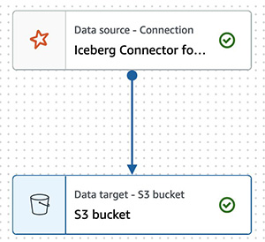
As depicted in Figure 1, mainframe data can be transferred via the secured network connection using AWS Transfer Family services or AWS DataSync to AWS cloud storage services, such as Amazon Elastic File System, Amazon Elastic Block Store, and Amazon Simple Storage Service (S3). After data is stored in AWS cloud, you can configure and move data among these services to meet with the business data processing need. Depending on data storage requirements, data storage costs can be further optimized by configuring S3 Lifecyle policies to move data among Amazon S3 storage classes. For long-term data archiving purpose, you can choose S3 Glacier storage class to achieve durability, resilience, and the optimal cost effectiveness.
Figure 1. Mainframe data backup and archival augmentation
Pattern 2: Augment mainframe with agile development and test environments including CI/CD pipeline on AWS
For any business-critical business application, a typical mainframe workload requires development and test environments to support production workloads. It’s common to see the lengthy application development lifecycle, a lack of automated testing, and an absent CI/CD pipeline with most of mainframes. Furthermore, the existing mainframe development processes and tools are outdated, as they are unable to keep up with the business pace, resulting in a growing backlog. Organizations with mainframes look for application development solutions to solve these challenges.
As demonstrated in Figure 2, AWS developer tools orchestrate code compilation, testing, and deployment among mainframe test environments. Mainframe test environments are either provided by the mainframe vendors as emulators or by AWS partners, such as Micro Focus. You can load the preferred developer tools and run an integrated development environment (IDE) from Amazon WorkSpaces or Amazon AppStream 2.0. Developers create or modify code in the IDE, and then commit and push their code to AWS CodeCommit. As soon as the code is pushed, an event is generated and triggers the pipeline in AWS CodePipeline to build the new code in a compilation environment via AWS CodeBuild. The pipeline pushes the new code to the test environment.
To optimize cost, you can scale the test environment capacity to meet needs. The tests are executed, and the test environment can be shut down when not in use. When the tests are successful, the pipeline pushes the code back to the mainframe via AWS CodeDeploy and an intermediary server. On the mainframe side, the code can go through a recompilation and final testing before being pushed to production.
You can further optimize operations and licensing cost of mainframe emulator by leveraging the managed integrated development and test environment provided by AWS Mainframe Modernization service.
Figure 2. Mainframe CI/CD augmentation
Pattern 3: Augment mainframe with agile data analytics on AWS
Core business applications running on mainframes generate a lot of data throughout the years. Decades of historical business transactions and massive amounts of user data present an opportunity to develop deep business insight. By creating a data lake using the AWS big data services, you can gain faster analytics capabilities and better insight into core business data originated from mainframe applications.
Figure 3 depicts data being pulled from relational, hierarchical, or mainframe file-based data stores on mainframes. These data are presented in various formats and stored as DB2 for z/OS, VSAM, IMS DB, IDMS, DMS, or other formats. You can use AWS partners data replication and change data capture tools from AWS Marketplace or AWS cloud services, such as Amazon Managed Streaming for Apache Kafka for near real-time data streaming, Transfer Family services, and DataSync for moving data in batch from mainframes to AWS.
Pattern 4: Augment mainframe with new functions and channels on AWS
Organizations with a mainframe use AWS to innovate and iterate quickly, as they often lack agility. For example, a common scenario for a bank could be providing a mobile application for customer engagements, such as supporting a marketing campaign for a new credit card.
As depicted in Figure 4, with the data replicated from mainframes to AWS cloud and analyzed by AWS big data and analytics services, new business functions can be developed on cloud-native applications by using Amazon API Gateway, AWS Lambda, and AWS Fargate. These new business applications can interact with mainframe data, and the combination can give deep business insight.
To add new innovation capabilities, with time-series data generated by the new business function applications, using Amazon Forecast can predict domain-specific metrics, such as inventory, workforce, web traffic, and finances. Amazon Lex can build virtual agents, automate informational response to customer enquiries, and improve business productivity. Adding Amazon SageMaker, you can prepare data gathered from mainframe and new business applications at scale to build, train, and deploy machine learning models for any business cases.
You can further improve customer engagement by incorporating Amazon Connect and Amazon Pinpoint to build multichannel communications.
Figure 4. Mainframe new functions and channels augmentation
Conclusion
To increase agility, maximize the value of investments, and innovate faster, organizations can adopt the patterns discussed in this post to augment mainframes by using AWS services to build resilient data protection solution, provision agile CI/CD integrated development and test environment, liberate mainframe data and developing innovation solutions for new digital customer experience. With AWS Mainframe Modernization service, you can accelerate this journey and innovate faster.
At Amazon Web Services (AWS) we prioritize security, performance, and strong encryption in our cloud services. In order to be prepared for quantum computer advancements, we’ve been investigating the use of quantum-safe algorithms for key exchange in the TLS protocol. In this blog post, we’ll first bring you up to speed on what we’ve been doing on the TLS front. Then, we’ll focus on the QUIC transport protocol and show how you can enable and experiment with the newly released post-quantum (PQ) key exchange by using our s2n-quic library. The s2n-quic library is an open-source implementation of the QUIC protocol.
Why use PQ-hybrid key establishment in s2n-quic?
A large-scale quantum computer could break the current public key cryptography that is used to establish keys for secure communication connections. Although a large-scale quantum computer isn’t available today, traffic that is recorded now could be decrypted by one in the future. With such concerns in mind, the recent US Congress Quantum Computing Cybersecurity Preparedness Act and the White House National Security Memorandum set a goal of a timely and equitable transition of cryptographic systems to quantum-resistant cryptography.
PQ-hybrid key establishment in TLS is a feature that introduces post-quantum KEMs used in conjunction with classical Elliptic Curve Diffie-Hellman (ECDH) key exchange. The client and server still do an ECDH key exchange. Additionally, the server encapsulates a post-quantum shared secret to the client’s post-quantum KEM public key, which is advertised in the ClientHello message. This strategy combines the high assurance of a classical key exchange with the security of the proposed post-quantum key exchanges, to ensure that the handshakes are protected as long as the ECDH or the post-quantum shared secret cannot be broken.
After decapsulating the secret, the client and server have an ECDH and a post-quantum shared secret, which they concatenate and use to derive the symmetric keys that are used in the Authenticated Encryption with Additional Data (AEAD) cipher in TLS. These symmetric keys used by the AEAD cipher for data encryption will be secure against a quantum computer, which means that the TLS communication is secure against a quantum computer. The AWS implementation of TLS is s2n-tls, a streamlined open source implementation of TLS. The s2n-tls implementation already supports PQ-hybrid key exchange with ECDH and three NIST PQC Project KEMs (Kyber, BIKE, and SIKE) for TLS 1.2 and 1.3. The use of KEMs for TLS 1.2 is described in the draft-campagna-tls-bike-sike-hybrid IETF draft, and the use of KEMs for TLS 1.3 is described in the draft-ietf-tls-hybrid-design IETF draft.
Note: The Kyber, BIKE, and SIKE implementations follow the algorithm specifications described in NIST PQ Project Round 3, which are expected to be updated as standardization proceeds.
How PQ-hybrid key exchange works in s2n-quic
AWS recently announceds2n-quic, an open-source Rust implementation of the QUIC protocol. QUIC is an encrypted transport protocol that is designed for performance and is the foundation of HTTP/3. For tunnel establishment, QUIC uses TLS 1.3 carried over QUIC transport. To alleviate the harvest-now-decrypt-later concerns for customers that use s2n-quic, in the next section we show you how to enable PQ-hybrid key establishment in s2n-quic. AWS services and software that use s2n-quic will automatically inherit the ability to support quantum-safe key exchanges in the future when post-quantum algorithms are standardized and are officially supported in s2n-quic.
The s2n-quic implementation is written in the Rust programming language. It can use either s2n-tls (the TLS library for AWS) or rustls (the TLS library in Rust) to perform the TLS handshake. If you build s2n-quic with s2n-tls, then s2n-quic inherits the post-quantum support that is offered in s2n-tls. In turn, s2n-tls is built over other crypto libraries such as the AWS libcrypto (AWS-LC) or alternatively OpenSSL crypto library (libcrypto). AWS-LC is a general-purpose cryptographic library that is maintained by AWS, which will incorporate standardized post-quantum algorithms. Therefore, building s2n-tls with AWS-LC will provide s2n-tls with the post-quantum cryptographic algorithms for use in s2n-quic.
Such a model allows for AWS services and software that use s2n-quic to automatically inherit the standardized post-quantum options as they are implemented in s2n-tls and its underlying crypto libraries. There will be no need to tweak s2n-quic to support post-quantum TLS 1.3 handshakes. The whole stack of protocol implementations is architected in an agile manner without duplication of work.
The public s2n-quic GitHub repository includes an example that demonstrates how to build the library with PQ-hybrid key exchange support, along with a server and client to test. The PQ-hybrid key exchange feature test requires CMake in Linux or macOS. The experiments below were run in an Amazon Linux 2 instance with rustc, Cargo, Clang, and CMake installed. Connections that you establish with this experimental build of s2n-quic will support PQ-hybrid key exchange.
To test PQ-hybrid key establishment
Clone s2n-quic by using the following commands:
git clone https://github.com/aws/s2n-quic cd s2n-quic
Run the example post-quantum s2n-quic client and server in the post-quantum directory to confirm that they negotiate a PQ-hybrid key by using the following commands:
cd examples/post-quantum cargo run –bin pq_server cargo run –bin pq_client
Note: Although these examples with the PQ-hybrid feature experimental build of s2n-quic are self-contained, if you want to manually change and build s2n-quic and s2n-tls to enable PQ-hybrid key exchange, you have to update the default_tls13 policy in s2n-tls to point to security_policy_pq_tls_1_0_2021_05_26 in tls/s2n_security_policies.c. Then you rebuild s2n-tls and override the location that s2n-quic links to by setting the S2N_TLS_DIR, S2N_TLS_LIB_DIR, and S2N_TLS_INCLUDE_DIR environment variables at build time.
To confirm the PQ-hybrid key establishment, you capture the QUIC negotiation by using the following tcpdump command:
sudo tcpdump -i lo port 4433 -w test.pcap
Open the capture by using a packet capture visualization application. First you look at the ClientHello message, as shown in the capture in Figure 1 taken from Wireshark.
Figure 1: pq_client ClientHello in QUIC
In the QUIC CRYPTO frame, you can see the TLS 1.3 cipher suites, and that the TLS version is 1.3 while the supported key exchange groups are classical ECDH (with identifiers 0x0017, 0x0018, 0x001d) and 0x2f39, 0x2f3a, 0x2f37…. 0x2f1f. The 0x2f… groups are the agreed upon identifiers (not standardized yet) for PQ-hybrid key exchange. You also see the PQ-hybrid X25519+Kyber512 (with identifier 12089 or 0x2f39) key share that is offered by the client. That key share includes 32 bytes for the Curve25519 ephemeral ECDH client public key, 800 bytes for the ephemeral Kyber512 public key, and 4 bytes for the identifier and the key share length.
Note: The post-quantum KEMs implementations at the time of this writing follow the NIST Round 3 Kyber, BIKE, and SIKE specifications. We expect these specifications to change as the NIST PQC Project proceeds with standardization. Post-quantum support in s2n-tls and s2n-quic will be experimental until NIST has selected and published standardized algorithms and identifiers. Pushing the change to the main branch now would mean that s2n-quic clients would be sending a PQ-hybrid key share that won’t be used until the servers on the internet start supporting it. The actual algorithms and their identifiers will still be integrated in future releases of s2n-tls and AWS-LC. Therefore, s2n-quic will still be able to negotiate the NIST and IETF standardized options. Meanwhile, we will continue to experiment with post-quantum QUIC and its potential challenges.
Next, take a look at the server-negotiated keys in the ServerHello message, as shown in Figure 2.
Figure 2: pq_server ServerHello in QUIC
You can again see the TLS 1.3 cipher suite, the TLS version being 1.3, and the picked PQ-hybrid X25519+Kyber512 key share. The key share includes 4 bytes for the identifier and the key share length, 32 bytes for the Curve25519 ephemeral ECDH server public key, and 768 bytes for the Kyber512 ciphertext that encapsulates a post-quantum shared secret to the client’s ephemeral Kyber512 public key (included in its ClientHello message).
The rest of the handshake completes successfully by deriving symmetric keys from the X25519 and Kyber512 post-quantum shared secrets (as defined in the draft-ietf-tls-hybrid-design IETF draft) and encrypting the rest of the messages with Advanced Encryption Standard with Galois/Counter Mode (AES-GCM) by using these symmetric keys over QUIC.
Benchmark
Now you can benchmark the post-quantum QUIC client and server by using netbench, a transport protocol benchmarking tool that is available in the s2n-quic repository.
To benchmark the post-quantum QUIC client and server
Go in the netbench directory and build it with the correct flags for the experimental post-quantum QUIC examples, by using the following commands:
cd s2n-quic/netbench RUSTFLAGS=”–cfg s2n_quic_unstable –cfg s2n_quic_enable_pq_tls” cargo build –release
Generate the netbench scenario by using the following commands:
In this example, you’re trying to create 10,000 sequential QUIC connections. The scenario opens a connection, sends a single byte, receives a single byte, closes it, and repeats 10,000 times.
The drivers read the request_response.json to run the scenario. Then the driver is wrapped in a collector that outputs statistics to another JSON file. At the end of all of the 10,000 runs, the cli feature is used to generate the report.
Figure 3 shows the performance results for X25519, X25519+Kyber512, X25519+BIKE-1, and X25519+SIKEp434 key exchange. All connections used an ECDSA P256 server certificate for authentication.
Figure 3: PQ-hybrid key exchange impact on QUIC connection rates
The x-axis is time in seconds. The y-axis is the number of times send is called—which, for 1 byte per connection, practically means that the diagram shows the connection establishment rate (per second). The absolute performance numbers in these benchmarks are not important, because the results could change based on the netbench scenario parameters. The performance difference between PQ-hybrid key exchange algorithms is what this graph is highlighting.
You can see that the classical X25519 achieves higher connection rates, because it is the most efficient option (that offers no post-quantum protection). The performance of Kyber is competitive and achieves 8% fewer connections per second when used with X25519 in a PQ-hybrid key exchange. BIKE-1 is relatively efficient, but adds some extra latency and introduces two frames for the ClientHello, which leads to 37% fewer connections per second. SIKEp434, although it offers much smaller public keys and ciphertexts, is orders of magnitude slower, which means it offers 95% fewer connections per second. These results match previous results we have shared before and other research works, where the most efficient signature algorithms ended up with higher connection rates and lower connection failure probabilities due to overload.
Conclusion
In this post, we showed how you can use s2n-quic in conjunction with s2n-tls to enable QUIC connections to negotiate encryption keys in a quantum-resistant manner. If you’re interested in learning more about s2n-quic, join us at AWS re:Inforce in July for the breakout session entitled NIS304: Using s2n-quic: Bringing QUIC, the secure transport protocol, to AWS.
As always, if you’re interested in using or contributing to s2n-quic, the source code and documentation are publicly available under the terms of the Apache Software License 2.0 from our s2n-quic GitHub repository. If you package or distribute s2n-quic or s2n-tls, or use it as part of a large multi-user service, you might be eligible for pre-notification of security issues. Contact [email protected] for more information. If you discover a potential security issue in s2n-quic or s2n-tls, we ask that you notify AWS Security by using our vulnerability reporting page.
If you have feedback about this post, submit comments in the Comments section below. If you have questions about this post, contact AWS Support.
Want more AWS Security news? Follow us on Twitter.
The AWS Cloud Development Kit (AWS CDK) is an open-source software development framework to define your cloud application resources using familiar programming languages. AWS CDK uses the familiarity and expressive power of programming languages for modeling your applications. Constructs are the basic building blocks of AWS CDK apps. A construct represents a “cloud component” and encapsulates everything that AWS CloudFormation needs to create the component. Furthermore, AWS Construct Library lets you ease the process of building your application using predefined templates and logic. Three levels of constructs exist:
L1 – These are low-level constructs called Cfn (short for CloudFormation) resources. They’re periodically generated from the AWS CloudFormation Resource Specification. The name pattern is CfnXyz, where Xyz is name of the resource. When using these constructs, you must configure all of the resource properties. This requires a full understanding of the underlying CloudFormation resource model and its corresponding attributes.
L2 – These represent AWS resources with a higher-level, intent-based API. They provide additional functionality with defaults, boilerplate, and glue logic that you’d be writing yourself with L1 constructs. AWS constructs offer convenient defaults and reduce the need to know all of the details about the AWS resources that they represent. This is done while providing convenience methods that make it simpler to work with the resources and as a result creating your application.
L3 – These constructs are called patterns. They’re designed to complete common tasks in AWS, often involving multiple types of resources.
In this post, I show a sample architecture and how the complexity of an AWS CDK application is reduced by using L2 constructs.
Overview of the sample architecture
This solution uses Amazon API Gateway, AWS Lambda, and Amazon DynamoDB. I implement a simple serverless web application. The application receives a POST request from a user via API Gateway and forwards it to a Lambda function using proxy integration. The Lambda function writes the request body to a DynamoDB table.
You can follow the instructions in the README file of the GitHub repository to deploy the stack. In the following walkthrough, I explain each logical unit and the differences when implementing it using L1 and L2 constructs. Before each code sample, I’ll show the path in the GitHub repository where you can find its source.
Create the DynamoDB table
First, I create a DynamoDB table to store the request content.
L1 construct
With L1 constructs, I must define each attribute of a table separately. For the DynamoDB table, these are keySchema, attributeDefinitions, and provisionedThroughput. They all require detailed CloudFormation knowledge, for example, how a keyType is defined.
The corresponding L2 construct lets me use the default values for readCapacity (5) and writeCapacity (5). To further reduce the complexity, I define the attributes and the partition key simultaneously. In addition, I utilize the dynamodb.AttributeType.STRING enum.
Next, I create a Lambda function which receives the request and stores the content in the DynamoDB table. The runtime code uses Node.js.
L1 construct
When creating a Lambda function using L1 construct, I must specify all of the properties at creation time – the business logic code location, runtime, and the function handler. This includes the role for the Lambda function to assume. As a result, I must provide the Attribute Resource Name (ARN) of the role. In the “Granting permissions” sections later in this post, I show how to create this role.
I can achieve the same result with less complexity by leveraging the NodejsFunction L2 construct for Lambda function. It sets a default version for Node.js runtime unless another one is explicitly specified. The construct creates a Lambda function with automatic transpiling and bundling of TypeScript or Javascript code. This results in smaller Lambda packages that contain only the code and dependencies needed to run the function, and it uses esbuild under the hood. The Lambda function handler code is located in the runtime directory of the API logical unit. I provide the path to the Lambda handler file in the entry property. I don’t have to specify the handler function name, because the NodejsFunction construct uses the handler name by default. Moreover, a Lambda execution role isn’t required to be provided during L2 Lambda construct creation. If no role is specified, then a default one is generated which has permissions for Lambda execution. In the section ‘Granting Permissions’, I describe how to customize the role after creating the construct.
Every step, from creating a new API Gateway REST API, to the deployment process, must be configured individually. With an L1 construct, I must have a good understanding of CORS and the exact configuration of headers and methods.
Furthermore, I must know all of the specifics, such as for the Lambda integration type I must know how to construct the URI.
Creating an API Gateway REST API with CORS enabled is simpler with L2 constructs. I can leverage the defaultCorsPreflightOptions property and the construct builds the required options method. To set origins and methods, I can use the apigateway.Cors enum. To configure the Lambda proxy option, all I need to do is to set the proxy variable in the method to true. A default deployment is created automatically.
In the sample application, I must give permissions to two different resources:
API Gateway REST API to invoke the Lambda function.
Lambda function to write data to the DynamoDB table.
L1 construct
For both resources, I must define AWS Identity and Access Management (IAM) roles. This requires in-depth knowledge of IAM, how policies are structured, and which actions are required. In the following code snippet, I start by creating the policy documents. Afterward, I create a role for each resource. These are provided at creation time to the corresponding constructs as shown earlier.
The database construct exposes a function to grant write access to any IAM role. The function creates a policy, which allows dynamodb:PutItem on the database table and adds it as an additional policy to the role.
At this point, all permissions are in place, except that Lambda function doesn’t have permissions to write data to the DynamoDB table yet. To grant write access, I call the grantWriteData function of the Database construct with the IAM role of the Lambda function.
lib/deployment.ts
database.grantWriteData(api.cfnLambdaIamRole)
L2 construct
Creating an API Gateway REST API with the LambdaIntegration construct generates the IAM role and attaches the role to the API Gateway REST API method. Giving the Lambda function permission to write to the DynamoDB table can be achieved with the following single line:
To reduce complexity even further, I can leverage L3 constructs. In the case of this sample architecture, I can utilize the LambdaRestApi construct. This construct uses a default Lambda proxy integration. It automatically generates a method and a deployment, and grants permissions. As a result, I can achieve the same with even less code.
Many services in this post are available in the AWS Free Tier. However, using this solution may incur costs, and you should tear down the stack if you don’t need it anymore. Cleanup steps are included in the RADME file of the GitHub repository.
Conclusion
In this post, I highlight the difference between using L1 and L2 AWS CDK constructs with an example architecture. Leveraging L2 constructs reduces the complexity of your application by using predefined patterns, boiler plate, and glue logic. They offer convenient defaults and reduce the need to know all of the details about the AWS resources they represent, while providing convenient methods that make it simpler to work with the resource. Additionally, I showed how to reduce complexity for common tasks even further by using an L3 construct.
Visit the AWS CDK documentation to learn more about building resilient, scalable, and cost-efficient architectures with the expressive power of a programming language.
Transactional data lake technologies such as Apache Hudi, Delta Lake, Apache Iceberg, and AWS Lake Formation governed tables is evolving rapidly, and gaining great popularity. These technologies simplified the data processing pipeline significantly, and they provided further useful capabilities like upserts, rolling back, and time travel queries.
In the first post of this series, we went through how to process Apache Hudi, Delta Lake, and Apache Iceberg datasets using AWS Glue connectors. AWS Glue simplifies reading and writing your data in those data lake formats, and building the data lakes on top of those technologies. Running the sample notebooks on AWS Glue Studio notebook, you could interactively develop and run your code, then immediately see the results. The notebooks let you explore how those technologies work when you have coding experience.
This second post focuses on other use cases for customers who prefer visual job authoring without writing custom code. Even without coding experience, you can easily build your transactional data lakes on AWS Glue Studio visual editor, and take advantage of those transactional data lake technologies. In addition, you can also use Amazon Athena to query the data stored using Hudi and Iceberg. This tutorial demonstrates how to read and write each format on AWS Glue Studio visual editor, and then how to query from Athena.
Process Apache Hudi, Delta Lake, Apache Iceberg dataset at scale
The following are the instructions to read/write tables using each data lake format on AWS Glue Studio Visual Editor. You can use any of the marketplace connector or the custom connector based on your requirements.
To continue this tutorial, you must create the following AWS resources in advance:
Reads/writes using the connector on AWS Glue Studio Visual Editor
In this tutorial, you read and write each of the transaction data lake format data on the AWS Glue Studio Visual Editor. There are three main configurations: connection, connection options, and job parameters that you must configure per the data lake format. Note that no code is included in this tutorial. Let’s see how it works.
Apache Hudi writes
Complete following steps to write into Apache Hudi table using the connector:
Open AWS Glue Studio.
Choose Jobs.
Choose Visual with a source and target.
For Source, choose Amazon S3.
For Target, choose hudi-0101-byoc-connector.
Choose Create.
Under Visual, choose Data source – S3 bucket.
Under Node properties, for S3 source type, choose S3 location.
For S3 URL, enter s3://covid19-lake/rearc-covid-19-world-cases-deaths-testing/json/.
Choose Data target – Connector.
Under Node properties, for Connection, choose hudi-0101-byoc-connection.
For Connection options, enter the following pairs of Key and Value (choose Add new option to enter a new pair).
Key: path. Value: <Your S3 path for Hudi table location>
Under Job details, for IAM Role, choose your IAM role.
Under Advanced properties, for Job parameters, choose Add new parameter.
For Key, enter --conf.
For Value, enter spark.serializer=org.apache.spark.serializer.KryoSerializer.
Choose Save.
Choose Run.
Apache Hudi reads
Complete following steps to read from the Apache Hudi table that you created in the previous section using the connector:
Open AWS Glue Studio.
Choose Jobs.
Choose Visual with a source and target.
For Source, choose hudi-0101-byoc-connector.
For Target, choose Amazon S3.
Choose Create.
Under Visual, choose Data source – Connection.
Under Node properties, for Connection, choose hudi-0101-byoc-connection.
For Connection options, choose Add new option.
For Key, enter path. For Value, enter your S3 path for your Hudi table that you created in the previous section.
Choose Transform – ApplyMapping, and choose Remove.
Choose Data target – S3 bucket.
Under Data target properties, for Format, choose JSON.
For S3 Target type. choose S3 location.
For S3 Target Location enter your S3 path for output location.
Under Job details, for IAM Role, choose your IAM role.
Choose Save.
Choose Run.
Delta Lake writes
Complete the following steps to write into the Delta Lake table using the connector:
Open AWS Glue Studio.
Choose Jobs.
Choose Visual with a source and target.
For Source, choose Amazon S3.
For Target, choose delta-100-byoc-connector.
Choose Create.
Under Visual, choose Data source – S3 bucket.
Under Node properties, for S3 source type, choose S3 location.
For S3 URL, enter s3://covid19-lake/rearc-covid-19-world-cases-deaths-testing/json/.
Choose Data target – Connector.
Under Node properties, for Connection, choose your delta-100-byoc-connection.
For Connection options, choose Add new option.
For Key, enter path. For Value, enter your S3 path for Delta table location. Choose Add new option.
For Key, enter partitionKeys. For Value, enter iso_code.
Under Job details, for IAM Role, choose your IAM role.
Under Advanced properties, for Job parameters, choose Add new parameter.
For Key, enter --conf.
For Value, enter spark.sql.extensions=io.delta.sql.DeltaSparkSessionExtension --conf spark.sql.catalog.spark_catalog=org.apache.spark.sql.delta.catalog.DeltaCatalog.
Choose Save.
Choose Run.
Delta Lake reads
Complete the following steps to read from the Delta Lake table that you created in the previous section using the connector:
Open AWS Glue Studio.
Choose Jobs.
Choose Visual with a source and target.
For Source, choose delta-100-byoc-connector.
For Target, choose Amazon S3.
Choose Create.
Under Visual, choose Data source – Connection.
Under Node properties, for Connection, choose delta-100-byoc-connection.
For Connection options, choose Add new option.
For Key, enter path. For Value, enter your S3 path for Delta table that you created in the previous section. Choose Add new option.
For Key, enter partitionKeys. For Value, enter iso_code.
Choose Transform – ApplyMapping, and choose Remove.
Choose Data target – S3 bucket.
Under Data target properties, for Format, choose JSON.
For S3 Target type, choose S3 location.
For S3 Target Location enter your S3 path for output location.
Under Job details, for IAM Role, choose your IAM role.
Under Advanced properties, for Job parameters, choose Add new parameter.
For Key, enter --conf.
For Value, enter spark.sql.extensions=io.delta.sql.DeltaSparkSessionExtension --conf spark.sql.catalog.spark_catalog=org.apache.spark.sql.delta.catalog.DeltaCatalog.
Choose Save.
Choose Run.
Apache Iceberg writes
Complete the following steps to write into Apache Iceberg table using the connector:
Open AWS Glue console.
Choose Databases.
Choose Add database.
For database name, enter iceberg, and choose Create.
Open AWS Glue Studio.
Choose Jobs.
Choose Visual with a source and target.
For Source, choose Amazon S3.
For Target, choose iceberg-0131-byoc-connector.
Choose Create.
Under Visual, choose Data source – S3 bucket.
Under Node properties, for S3 source type, choose S3 location.
For S3 URL, enter s3://covid19-lake/rearc-covid-19-world-cases-deaths-testing/json/.
Choose Data target – Connector.
Under Node properties, for Connection, choose iceberg-0131-byoc-connection.
For Connection options, choose Add new option.
For Key, enter path. For Value, enter glue_catalog.iceberg.test.
Choose SQL under Transform to create a new AWS Glue Studio node.
Under Node properties, for Node parents, choose ApplyMapping.
Under Transform, for SQL alias, verify that myDataSource is entered.
For SQL query, enter CREATE TABLE glue_catalog.iceberg.test AS SELECT * FROM myDataSource WHERE 1=2. This is to create a table definition with no records because the Iceberg target requires table definition before data ingestion.
Under Job details, for IAM Role, choose your IAM role.
Under Advanced properties, for Job parameters, choose Add new parameter.
For Key, enter --conf.
For Value, enter the following value (replace the placeholder your_s3_bucket with your S3 bucket name): spark.sql.catalog.glue_catalog=org.apache.iceberg.spark.SparkCatalog --conf spark.sql.catalog.glue_catalog.warehouse=s3://your_s3_bucket/iceberg/warehouse --conf spark.sql.catalog.glue_catalog.catalog-impl --conf park.sql.catalog.glue_catalog.io-impl=org.apache.iceberg.aws.s3.S3FileIO --conf spark.sql.catalog.glue_catalog.lock-impl=org.apache.iceberg.aws.glue.DynamoLockManager --conf spark.sql.catalog.glue_catalog.lock.table=iceberg_lock --conf spark.sql.extensions=org.apache.iceberg.spark.extensions.IcebergSparkSessionExtensions
Choose Save.
Choose Run.
Apache Iceberg reads
Complete the following steps to read from Apache Iceberg table that you created in the previous section using the connector:
Open AWS Glue Studio.
Choose Jobs.
Choose Visual with a source and target.
For Source, choose Apache Iceberg Connector for AWS Glue 3.0.
For Target, choose Amazon S3.
Choose Create.
Under Visual, choose Data source – Connection.
Under Node properties, for Connection, choose your Iceberg connection name.
For Connection options, choose Add new option.
For Key, enter path. For Value, enter glue_catalog.iceberg.test.
Choose Transform – ApplyMapping, and choose Remove.
Choose Data target – S3 bucket.
Under Data target properties, for Format, choose JSON.
For S3 Target type, choose S3 location.
For S3 Target Location enter your S3 path for the output location.
Under Job details, for IAM Role, choose your IAM role.
Under Advanced properties, for Job parameters, choose Add new parameter.
For Key, enter --conf.
For Value, enter the following value (replace the placeholder your_s3_bucket with your S3 bucket name): spark.sql.catalog.glue_catalog=org.apache.iceberg.spark.SparkCatalog --conf spark.sql.catalog.glue_catalog.warehouse=s3://your_s3_bucket/iceberg/warehouse --conf spark.sql.catalog.glue_catalog.catalog-impl --conf park.sql.catalog.glue_catalog.io-impl=org.apache.iceberg.aws.s3.S3FileIO --conf spark.sql.catalog.glue_catalog.lock-impl=org.apache.iceberg.aws.glue.DynamoLockManager --conf spark.sql.catalog.glue_catalog.lock.table=iceberg_lock --conf spark.sql.extensions=org.apache.iceberg.spark.extensions.IcebergSparkSessionExtensions
Choose Save.
Choose Run.
Query from Athena
The Hudi table and the iceberg tables created with the above instructions are also queryable from Athena.
This post summarized how to utilize Apache Hudi, Delta Lake, and Apache Iceberg on AWS Glue platform, as well as demonstrated how each format works with the AWS Glue Studio Visual Editor. You can start using those data lake formats easily in any of the AWS Glue DynamicFrames, Spark DataFrames, and Spark SQL on the AWS Glue jobs, the AWS Glue Studio notebooks, and the AWS Glue Studio visual editor.
About the Author
Noritaka Sekiyama is a Principal Big Data Architect on the AWS Glue team. He enjoys collaborating with different teams to deliver results like this post. In his spare time, he enjoys playing video games with his family.
In this blog post, you’ll learn how to extend the solution so you can use AWS Chatbot to remediate the findings in your Slack channel. You’ll receive the findings from Security Hub and then run AWS CLI commands from your Slack channel to remediate the reported security findings.
AWS Chatbot works by acting as a subscriber to an Amazon Simple Notification Service (Amazon SNS) topic that can receive notifications from either Amazon CloudWatch or Amazon EventBridge, and have them delivered to the configured Slack channels or Amazon Chime chat rooms. You can apply standard AWS Identity and Access Management (IAM) permissions to the Slack channel or Amazon Chime chatroom, and you can also associate some channel guardrails to provide granular control on what commands can be run from the channel. For example, you may want to allow running commands that would allow getting more details on findings reported from Security Hub, and remediating and archiving those findings, but use channel guardrails to prevent anyone from disabling Security Hub. Another example is that you might want to allow the channel members to query AWS CloudTrail logs in order to get more details on findings, but you use channel guardrails to prevent them from disabling AWS CloudTrail or changing the destination Amazon Simple Storage Services (Amazon S3) bucket.
Overview of ChatOps and ChatSecOps concepts
ChatOps, also known as Chat Operations, refers to using chatbots, tools, and clients to communicate, notify, assign, and launch operational tasks and issues. You can use your existing Slack channels and Amazon Chime chatrooms to receive alerts and notifications about operational issues or tasks, and you can also respond to those incidents or tasks in real time from the same chat room. SecOps is a philosophy of encouraging collaboration between the ITOps and Security teams of an organization. ChatSecOps, also known as Chat Security Operations, uses the ChatOps technology to enable customers to put SecOps in practice.
ChatSecOps facilitates this collaboration by allowing security-related notifications to be delivered to common chat rooms used by SecOps teams, providing visibility on the issues and actions that are taken to investigate and remediate the reported issues. SecOps teams can share threat analysis reports, compliance finding reports, and information on security vulnerabilities in these channels and work closely with DevOps teams to perform further analysis, investigation, and remediation of the issues and findings. This helps to ensure visibility and collaboration across the SecOps and DevOps teams and promotes the philosophy of DevSecOps.
Prerequisites
To get started, you’ll need the following prerequisites:
You need to grant permissions to the users in Slack channels, which you can do in one of the following ways:
Associate a channel IAM role with AWS Chatbot. This method provides similar permissions to all the members of the Slack channel. A channel IAM role is more useful if all your channel members require the same set of permissions. The channel IAM role can also be used to restrict the permissions provided by the user IAM role.
Define user roles. User roles require channel members to choose their own roles. This allows different users in your channel to have different sets of permissions. User roles are also useful when you don’t want new channel members to perform actions as soon as they join the channel.
For detailed instructions about setting up AWS Chatbot and defining permissions, see Getting started with AWS Chatbot. For more information about setting boundaries on the permissions that can be allowed by the channel and user IAM roles, see Channel guardrails.
Integrate the Slack channel with AWS Chatbot
After you set up the Slack channel with required permissions, you integrate the ChatOps for AWS app with your channel by using the following steps.
To integrate the Slack channel with AWS Chatbot
Log in to Slack by using either the Slack app or web browser.
In the Slack sidebar, from the Channels section, choose the channel name.
In the right pane, choose the channel name to open the channel configuration window.
Choose the Integrations tab, then choose Add an App.
In the search bar, enter AWS Chatbot. In the search results list, choose the Add button for AWS Chatbot.
On the Integrations tab, under Apps, you should see ChatOps for AWS, as shown in Figure 1.
Figure 1: Integrate the ChatOps for AWS app with your Slack channel
Now you’re ready to start running the commands. Note that you need to add @aws before writing any commands. For more information , see Running AWS CLI commands from Slack channels.
Use case: Amazon S3 Block Public Access enabled at the account level
The Amazon S3 Block Public Access feature provides settings for access points, buckets, and accounts to help you manage public access to Amazon S3 resources. With S3 Block Public Access, account administrators and bucket owners can set up centralized controls to limit public access to your S3 resources. These controls are enforced regardless of how the resources are created.
Amazon GuardDuty tracks and reports S3 Block Public Access feature configurations at the account level, as well as the bucket level. These findings are automatically sent to Security Hub.
To remediate finding for Amazon S3 Block Public Access from the Slack channel
You receive a Security Hub notification that Amazon S3 Block Public Access was disabled for an account in your designated Slack channel.
Figure 2: Notification received from Security Hub in Slack channel
This notification indicates that S3 Block Public Access was disabled for a specific account.
Note: Your Slack channel members require permissions to investigate and remediate the findings received in the Slack channel. As described earlier, you can grant permissions using a channel IAM role or a user IAM role. You should follow the principal of least privilege access when granting access and use IAM Access Analyzer to review the permissions that are granted through the channel or user IAM role.
Before you take any action, you need to find the current S3 Block Public Access configuration for the account. To do this, run the following AWS CLI command from the Slack channel, replacing <your_account_id> with the AWS account ID you are investigating.
Figure 3: AWS CLI command output in Slack channel indicating that S3 Block Public Access is disabled
You see that the output in Figure 3 shows that all the parameters of PublicAccessBlockConfiguration are set to false, which indicates that the Block Public Access feature is disabled at the account level.
To remediate this issue, run the following AWS CLI command in your Slack channel, replacing <your_account_id> with the AWS account ID you are investigating.
In the response from AWS Chatbot, look for Result was null to verify that the command was run without any errors.
Figure 4: AWS CLI command run from Slack channel to enable S3 Block Public Access
To check the current status of the configuration, and to validate whether the issue has been resolved, again run the following AWS CLI command from the Slack channel, replacing <your_account_id> with the AWS account ID you are investigating:
In the response, you see that all the parameters of PublicAccessBlockConfiguration are set to false, which indicates that the Block Public Access feature is enabled at the account level.
Figure 5: AWS CLI command output in Slack channel indicating S3 Block Public Access is enabled
Another example use case is that you get a security finding notifying you about unencrypted Amazon Elastic Block Store (Amazon EBS) volumes. You can remediate the finding by running AWS CLI commands to encrypt the volume. In addition to interacting with AWS services by running standard AWS CLI commands in the Slack channel, you can further extend this capability to run operating system (OS)-level commands by using AWS Systems Manager runbooks, using the same mechanism described in this post. For more information, see AWS Systems Manager Runbooks in the AWS Chatbot Administrator Guide.
Conclusion
In this blog post, you learned how to run AWS CLI commands from Slack channels to remediate your security findings. This allows you to receive alerts and notifications from Security Hub and other security services such as Amazon GuardDuty, then investigate and remediate the issues from a single platform. You can integrate AWS Chatbot with your security operation team’s Slack channel or Amazon Chime chatroom, and manage your security operations in a more collaborative, transparent, and automated manner.
If you have any questions about this post, let us know in the Comments section below. For more information about AWS Chatbot, see the AWS Chatbot Administrator Guide.
Want more AWS Security news? Follow us on Twitter.
The collective thoughts of the interwebz
Manage Consent
To provide the best experiences, we use technologies like cookies to store and/or access device information. Consenting to these technologies will allow us to process data such as browsing behavior or unique IDs on this site. Not consenting or withdrawing consent, may adversely affect certain features and functions.
Functional
Always active
The technical storage or access is strictly necessary for the legitimate purpose of enabling the use of a specific service explicitly requested by the subscriber or user, or for the sole purpose of carrying out the transmission of a communication over an electronic communications network.
Preferences
The technical storage or access is necessary for the legitimate purpose of storing preferences that are not requested by the subscriber or user.
Statistics
The technical storage or access that is used exclusively for statistical purposes.The technical storage or access that is used exclusively for anonymous statistical purposes. Without a subpoena, voluntary compliance on the part of your Internet Service Provider, or additional records from a third party, information stored or retrieved for this purpose alone cannot usually be used to identify you.
Marketing
The technical storage or access is required to create user profiles to send advertising, or to track the user on a website or across several websites for similar marketing purposes.