Tag Archives: Advanced (300)

How to revoke federated users’ active AWS sessions

Post Syndicated from Matt Howard original https://aws.amazon.com/blogs/security/how-to-revoke-federated-users-active-aws-sessions/

When you use a centralized identity provider (IdP) for human user access, changes that an identity administrator makes to a user within the IdP won’t invalidate the user’s existing active Amazon Web Services (AWS) sessions. This is due to the nature of session durations that are configured on assumed roles. This situation presents a challenge for identity administrators.

In this post, you’ll learn how to revoke access to specific users’ sessions on AWS assumed roles through the use of AWS Identity and Access Management (IAM) policies and service control policies (SCPs) via AWS Organizations.

Session duration overview

When you configure IAM roles, you have the option of configuring a maximum session duration that specifies how long a session is valid. By default, the temporary credentials provided to the user will last for one hour, but you can change this to a value of up to 12 hours.

When a user assumes a role in AWS by using their IdP credentials, that role’s credentials will remain valid for the length of their session duration. It’s convenient for end users to have a maximum session duration set to 12 hours, because this prevents their sessions from frequently timing out and then requiring re-login. However, a longer session duration also poses a challenge if you, as an identity administrator, attempt to revoke or modify a user’s access to AWS from your IdP.

For example, user John Doe is leaving the company and you want to verify that John has his privileges within AWS revoked. If John has access to IAM roles with long-session durations, then he might have residual access to AWS despite having his session revoked or his user identity deleted within the IdP. Perhaps John assumed a role for his daily work at 8 AM and then you revoked his credentials within the IdP at 9 AM. Because John had already assumed an AWS role, he would still have access to AWS through that role for the duration of the configured session, 8 PM if the session was configured for 12 hours. Therefore, as a security best practice, AWS recommends that you do not set the session duration length longer than is needed. This example is displayed in Figure 1.

Figure 1: Session duration overview

Figure 1: Session duration overview

In order to restrict access despite the session duration being active, you could update the roles that are assumable from an IdP with a deny-all policy or delete the role entirely. However, this is a disruptive action for the users that have access to this role. If the role was deleted or the policy was updated to deny all, then users would no longer be able to assume the role or access their AWS environment. Instead, the recommended approach is to revoke access based on the specific user’s principalId or sourceIdentity values.

The principalId is the unique identifier for the entity that made the API call. When requests are made with temporary credentials, such as assumed roles through IdPs, this value also includes the session name, such as [email protected]. The sourceIdentity identifies the original user identity that is making the request, such as a user who is authenticated through SAML federation from an IdP. As a best practice, AWS recommends that you configure this value within the IdP, because this improves traceability for user sessions within AWS. You can find more information on this functionality in the blog post, How to integrate AWS STS SourceIdentity with your identity provider.

Identify the principalId and sourceIdentity by using CloudTrail

You can use AWS CloudTrail to review the actions taken by a user, role, or AWS service that are recorded as events. In the following procedure, you will use CloudTrail to identify the principalId and sourceIdentity contained in the CloudTrail record contents for your IdP assumed role.

To identify the principalId and sourceIdentity by using CloudTrail

  1. Assume a role in AWS by signing in through your IdP.
  2. Perform an action such as a creating an S3 bucket.
  3. Navigate to the CloudTrail service.
  4. In the navigation pane, choose Event History.
  5. For Lookup attributes, choose Event name. For Event name, enter CreateBucket.
  6. Figure 2: Looking up the CreateBucket event in the CloudTrail event history

    Figure 2: Looking up the CreateBucket event in the CloudTrail event history

  7. Select the corresponding event record and review the event details. An example showing the userIdentity element is as follows.

"userIdentity": {
	"type": "AssumedRole",
	"principalId": 
"AROATVGBKRLCHXEXAMPLE:[email protected]",
	"arn": "arn:aws:sts::111122223333:assumed-
role/roleexample/[email protected]",
	"accountId": "111122223333",
	"accessKeyId": "ASIATVGBKRLCJEXAMPLE",
	"sessionContext": {
		"sessionIssuer": {
			"type": "Role",
			"principalId": "AROATVGBKRLCHXEXAMPLE",
			"arn": 
"arn:aws:iam::111122223333:role/roleexample",
			"accountId": "111122223333",
			"userName": "roleexample"
		},
		"webIdFederationData": {},
		"attributes": {
			"creationDate": "2022-07-05T15:48:28Z",
			"mfaAuthenticated": "false"
		},
		"sourceIdentity": "[email protected]"
	}
}

In this event record, you can see that principalId is “AROATVGBKRLCHXEXAMPLE:[email protected]” and sourceIdentity was specified as “[email protected]”. Now that you have these values, let’s explore how you can revoke access by using SCP and IAM policies.

Use an SCP to deny users based on IdP user name or revoke session token

First, you will create an SCP, a policy that can be applied to an organization to offer central control of the maximum available permissions across the accounts in the organization. More information on SCPs, including steps to create and apply them, can be found in the AWS Organizations User Guide.

The SCP will have a deny-all statement with a condition for aws:userid, which will evaluate the principalId field; and a condition for aws:SourceIdentity, which will evaluate the sourceIdentity field. In the following example SCP, the users John Doe and Mary Major are prevented from accessing AWS, in member accounts, regardless of their session duration, because each action will check against their aws:userid and aws:SourceIdentity values and be denied accordingly.

SCP to deny access based on IdP user name


{
	"Version": "2012-10-17",
	"Statement": [
		{
			"Effect": "Deny",
			"Action": "*",
			"Resource": "*",
			"Condition": {
				"StringLike": {
					"aws:userid": [
						"*:[email protected]",
						"*:[email protected]"
				]
			}
		}
	},
	{
			"Effect": "Deny",
			"Action": "*",
			"Resource": "*",
			"Condition": {
				"StringEquals": {
					"aws:SourceIdentity": [
						"[email protected]",
						"[email protected]"
					]
				}
			}
		}
	]
}

Use an IAM policy to revoke access in the AWS Organizations management account

SCPs do not affect users or roles in the AWS Organizations management account and instead only affect the member accounts in the organization. Therefore, using an SCP alone to deny access may not be sufficient. However, identity administrators can revoke access in a similar way within their management account by using the following procedure.

To create an IAM policy in the management account

  1. Sign in to the AWS Management Console by using your AWS Organizations management account credentials.
  2. Follow these steps to use the JSON policy editor to create an IAM policy. Use the JSON of the SCP shown in the preceding section, SCP to deny access based on IdP user name, in the IAM JSON editor.
  3. Follow these steps to add the IAM policy to roles that IdP users may assume within the account.

Revoke active sessions when role chaining

At this point, the user actions on the IdP assumable roles within the AWS organization have been blocked. However, there is still an edge case if the target users use role chaining (use an IdP assumedRole credential to assume a second role) that uses a different RoleSessionName than the one assigned by the IdP. In a role chaining situation, the users will still have access by using the cached credentials for the second role.

This is where the sourceIdentity field is valuable. After a source identity is set, it is present in requests for AWS actions that are taken during the role session. The value that is set persists when a role is used to assume another role (role chaining). The value that is set cannot be changed during the role session. Therefore, it’s recommended that you configure the sourceIdentity field within the IdP as explained previously. This concept is shown in Figure 3.

Figure 3: Role chaining with sourceIdentity configured

Figure 3: Role chaining with sourceIdentity configured

A user assumes an IAM role via their IdP (#1), and the CloudTrail record displays sourceIdentity: [email protected] (#2). When the user assumes a new role within AWS (#3), that CloudTrail record continues to display sourceIdentity: [email protected] despite the principalId changing (#4).

However, if a second role is assumed in the account through role chaining and the sourceIdentity is not set, then it’s recommended that you revoke the issued session tokens for the second role. In order to do this, you can use the SCP policy at the end of this section, SCP to revoke active sessions for assumed roles. When you use this policy, the issued credentials related to the roles specified will be revoked for the users currently using them, and only users who were not denied through the previous SCP or IAM policies restricting their aws:userid will be able to reassume the target roles to obtain a new temporary credential.

If you take this approach, you will need to use an SCP to apply across the organization’s member accounts. The SCP must have the human-assumable roles for role chaining listed and a token issue time set to a specific time when you want users’ access revoked. (Normally, this time window would be set to the present time to immediately revoke access, but there might be circumstances in which you wish to revoke the access at a future date, such as when a user moves to a new project or team and therefore requires different access levels.) In addition, you will need to follow the same procedures in your management account by creating a customer-managed policy by using the same JSON with the condition statement for aws:PrincipalArn removed. Then attach the customer managed policy to the individual roles that are human-assumable through role chaining.

SCP to revoke active sessions for assumed roles


{
	"Version": "2012-10-17",
	"Statement": [
		{
			"Sid": "RevokeActiveSessions",
			"Effect": "Deny",
			"Action": [
				"*"
			],
			"Resource": [
				"*"
			],
			"Condition": {
				"StringEquals": {
					"aws:PrincipalArn": [
						"arn:aws:iam::<account-id>:role/<role-name>",
						"arn:aws:iam::<account-id>:role/<role-name>"
					]
				},
				"DateLessThan": {
					"aws:TokenIssueTime": "2022-06-01T00:00:00Z"
				}
			}
		}
	]
}

Conclusion and final recommendations

In this blog post, I demonstrated how you can revoke a federated user’s active AWS sessions by using SCPs and IAM policies that restrict the use of the aws:userid and aws:SourceIdentity condition keys. I also shared how you can handle a role chaining situation with the aws:TokenIssueTime condition key.

This exercise demonstrates the importance of configuring the session duration parameter on IdP assumed roles. As a security best practice, you should set the session duration to no longer than what is needed to perform the role. In some situations, that could mean an hour or less in a production environment and a longer session in a development environment. Regardless, it’s important to understand the impact of configuring the maximum session duration in the user’s environment and also to have proper procedures in place for revoking a federated user’s access.

This post also covered the recommendation to set the sourceIdentity for assumed roles through the IdP. This value cannot be changed during role sessions and therefore persists when a user conducts role chaining. Following this recommendation minimizes the risk that a user might have assumed another role with a different session name than the one assigned by the IdP and helps prevent the edge case scenario of revoking active sessions based on TokenIssueTime.

You should also consider other security best practices, described in the Security Pillar of the AWS Well-Architected Framework, when you revoke users’ AWS access. For example, rotating credentials such as IAM access keys in situations in which IAM access keys are regularly used and shared among users. The example solutions in this post would not have prevented a user from performing AWS actions if that user had IAM access keys configured for a separate IAM user in the environment. Organizations should limit long-lived security credentials such as IAM keys and instead rotate them regularly or avoid their use altogether. Also, the concept of least privilege is highly important to limit the access that users have and scope it solely to the requirements that are needed to perform their job functions. Lastly, you should adopt a centralized identity provider coupled with the AWS IAM Identity Center (successor to AWS Single Sign-On) service in order to centralize identity management and avoid the need for multiple credentials for users.

If you have feedback about this post, submit comments in the Comments section below. If you have questions about this post, start a new thread on the AWS Identity and Access Management re:Post or contact AWS Support.

Want more AWS Security news? Follow us on Twitter.
Author

Matt Howard

Matt is a Principal Technical Account Manager (TAM) for AWS Enterprise Support. As a TAM, Matt provides advocacy and technical guidance to help customers plan and build solutions using AWS best practices. Outside of AWS, Matt enjoys spending time with family, sports, and video games.

Setting up a secure CI/CD pipeline in a private Amazon Virtual Private Cloud with no public internet access

Post Syndicated from MJ Kubba original https://aws.amazon.com/blogs/devops/setting-up-a-secure-ci-cd-pipeline-in-a-private-amazon-virtual-private-cloud-with-no-public-internet-access/

With the rise of the cloud and increased security awareness, the use of private Amazon VPCs with no public internet access also expanded rapidly. This setup is recommended to make sure of proper security through isolation. The isolation requirement also applies to code pipelines, in which developers deploy their application modules, software packages, and other dependencies and bundles throughout the development lifecycle. This is done without having to push larger bundles from the developer space to the staging space or the target environment. Furthermore, AWS CodeArtifact is used as an artifact management service that will help organizations of any size to securely store, publish, and share software packages used in their software development process.

We’ll walk through the steps required to build a secure, private continuous integration/continuous development (CI/CD) pipeline with no public internet access while maintaining log retention in Amazon CloudWatch. We’ll utilize AWS CodeCommit for source, CodeArtifact for the Modules and software packages, and Amazon Simple Storage Service (Amazon S3) as artifact storage.

Prerequisites

The prerequisites for following along with this post include:

  • An AWS Account
  • A Virtual Private Cloud (Amazon VPC)
  • A CI/CD pipeline – This can be CodePipeline, Jenkins or any CI/CD tool you want to integrate CodeArtifact with, we will use CodePipeline in our walkthrough here.

Solution walkthrough

The main service we’ll focus on is CodeArtifact, a fully managed artifact repository service that makes it easy for organizations of any size to securely store, publish, and share software packages used in their software development process. CodeArtifact works with commonly used package managers and build tools, such as Maven and Gradle (Java), npm and yarn (JavaScript), pip and twine (Python), or NuGet (.NET).

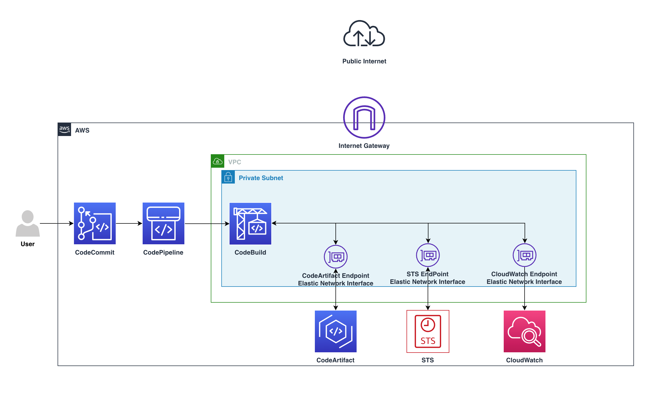
user checkin code to CodeCommit, CodePipeline will detect the change and start the pipeline, in CodeBuild the build stage will utilize the private endpoints and download the software packages needed without the need to go over the internet.

Users push code to CodeCommit, CodePipeline will detect the change and start the pipeline, in CodeBuild the build stage will utilize the private endpoints and download the software packages needed without the need to go over the internet.

The preceding diagram shows how the requests remain private within the VPC and won’t go through the Internet gateway, by going from CodeBuild over the private endpoint to CodeArtifact service, all within the private subnet.

The requests will use the following VPC endpoints to connect to these AWS services:

  • CloudWatch Logs endpoint (for CodeBuild to put logs in CloudWatch)
  • CodeArtifact endpoints
  • AWS Security Token Service (AWS STS) endpoint
  • Amazon Simple Storage Service (Amazon S3) endpoint

Walkthrough

  1. Create a CodeCommit Repository:
    1. Navigate to your CodeCommit Console then click on Create repository
Screenshot: Create repository button

Figure 2. Screenshot: Create repository button.

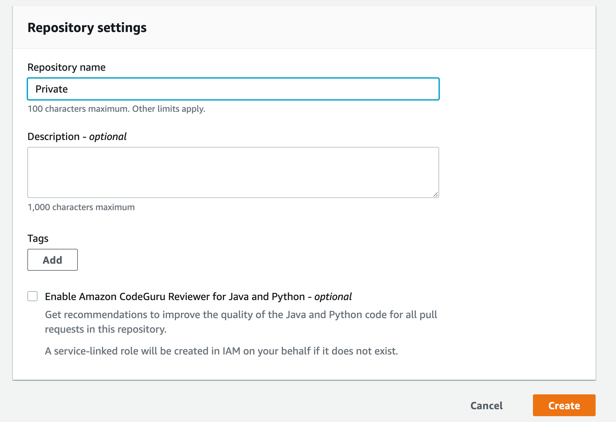
    1. Type in name for the repository then click Create
Screenshot: Repository setting with name shown as "Private" and empty Description

Figure 3. Screenshot: Repository setting with name shown as “Private” and empty Description.

    1. Scroll down and click Create file
Figure 4. Create file button.

Figure 4. Create file button.

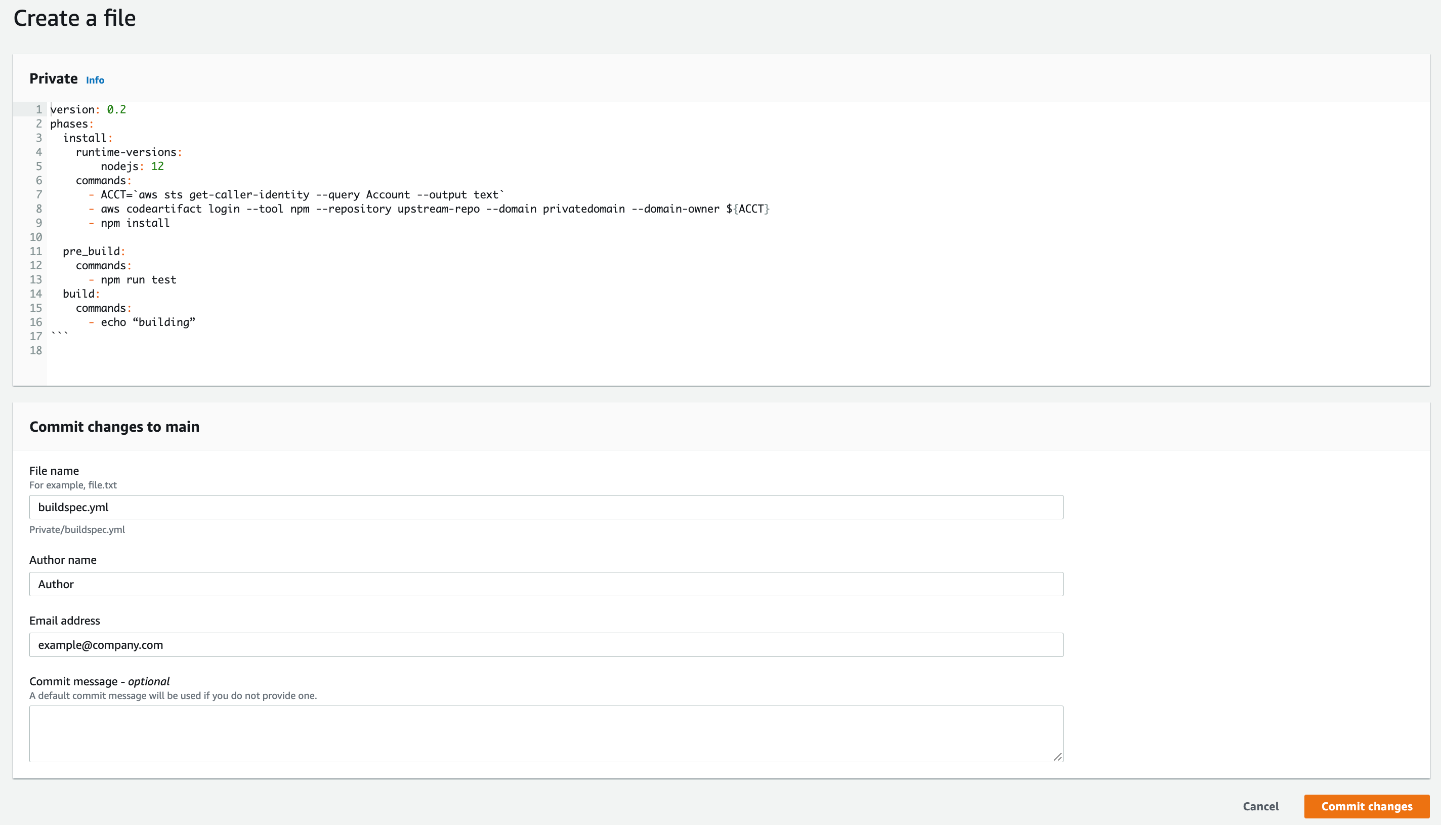
    1. Copy the example buildspec.yml file and paste it to the editor

Example buildspec.yml file:

version: 0.2
phases:
  install:
    runtime-versions:
        nodejs: 16
    
commands:
      - export AWS_STS_REGIONAL_ENDPOINTS=regional
      - ACCT=`aws sts get-caller-identity --region ${AWS_REGION} --query Account --output text`
      - aws codeartifact login --tool npm --repository Private --domain private --domain-owner ${ACCT}
      - npm install
  build:
    commands:
      - node index.js
    1. Name the file buildspec.yml, type in your name and your email address then Commit changes
Figure 5. Screenshot: Create file page.

Figure 5. Screenshot: Create file page.

  1. Create CodeArtifact
    1. Navigate to your CodeArtifact Console then click on Create repository
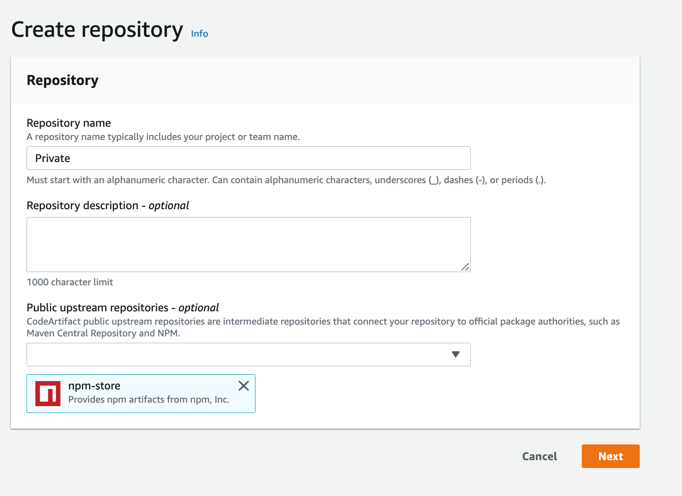
    2. Give it a name and select npm-store as public upsteam repository
Figure 6. Screenshot: Create repository page with Repository name "Private".

Figure 6. Screenshot: Create repository page with Repository name “Private”.

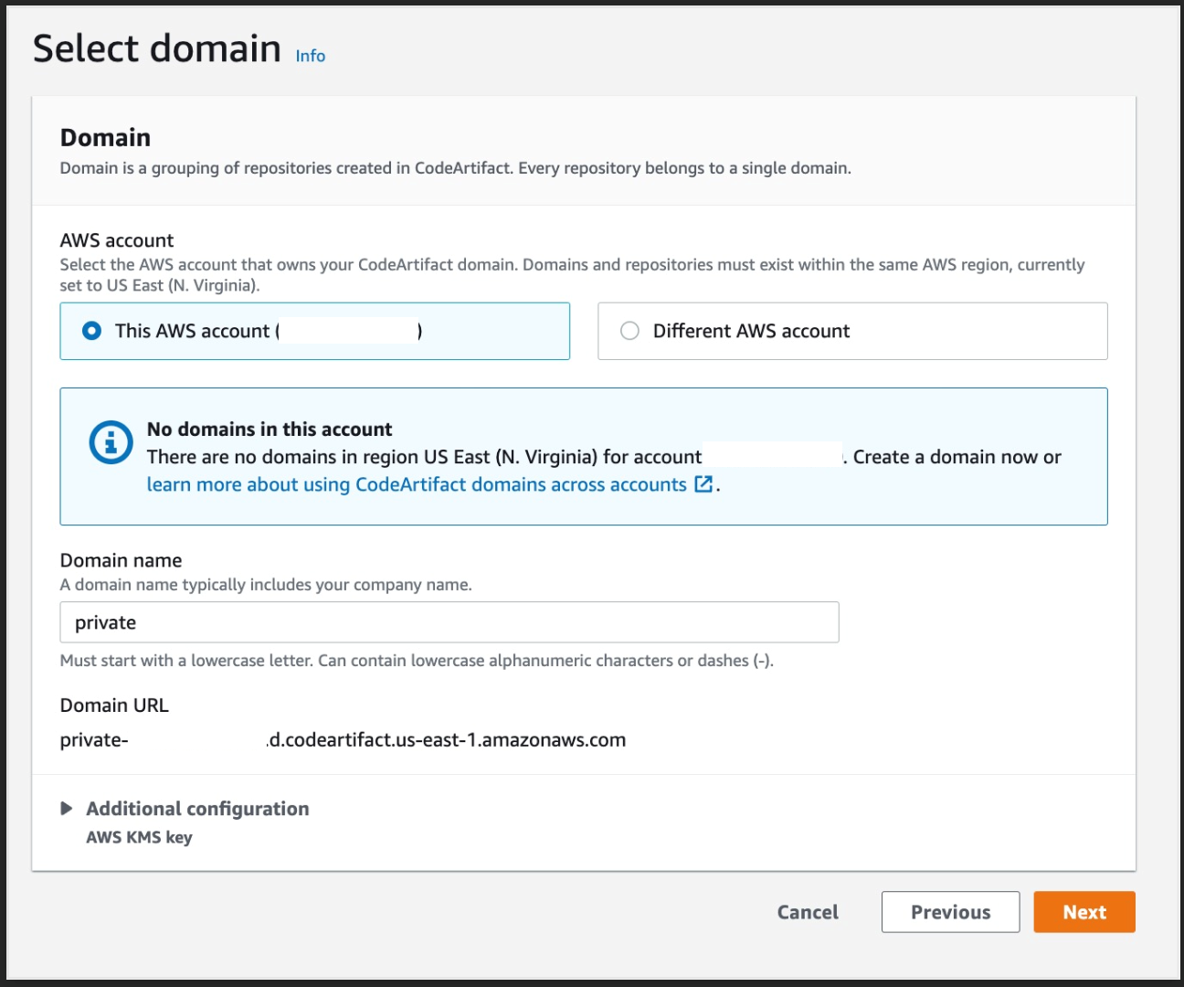
    1. For the Domain Select this AWS account and enter a domain name
Figure 7. Screenshot: Select domain page.

Figure 7. Screenshot: Select domain page.

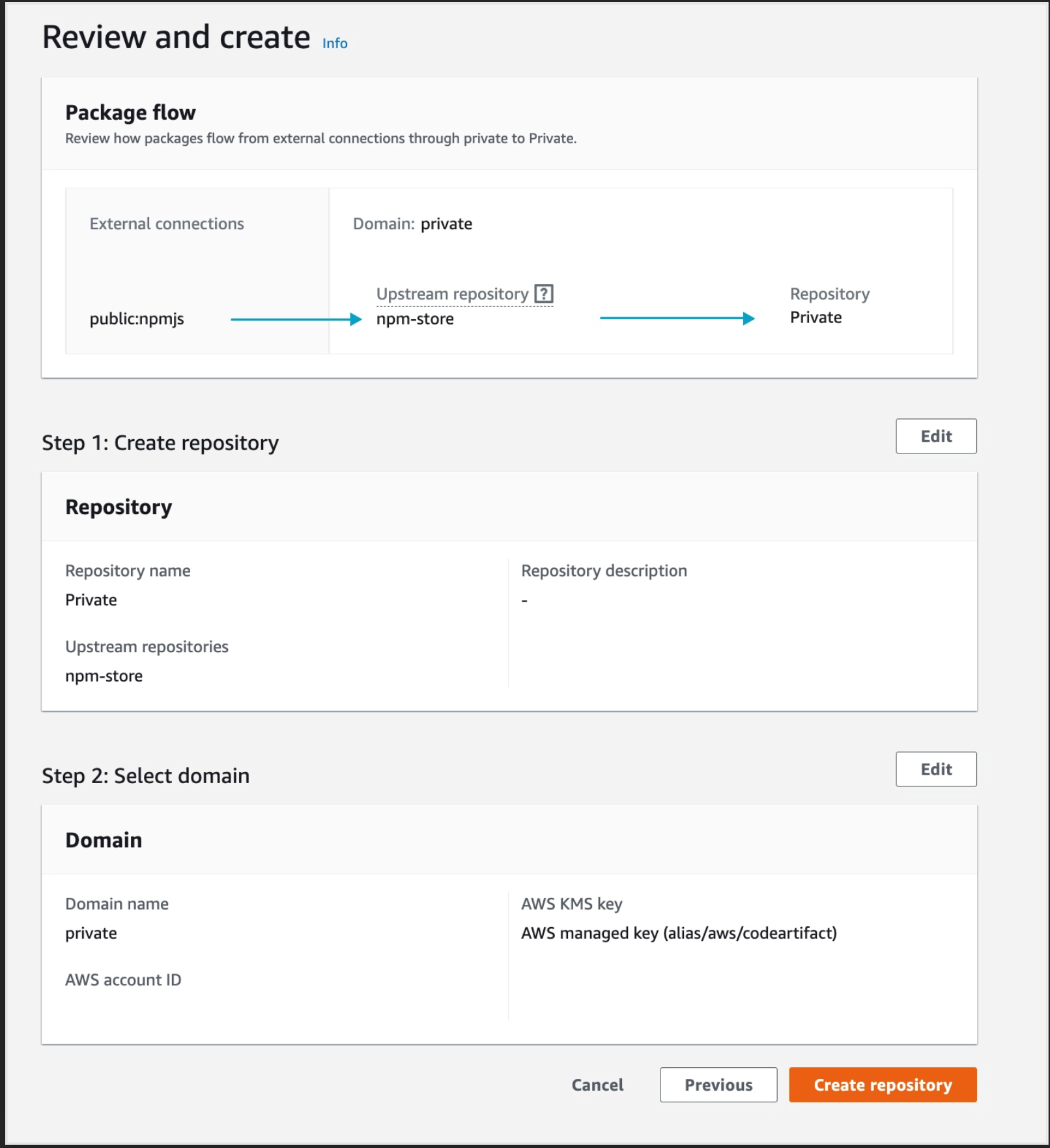
    1. Click Next then Create repository
Figure 8. Screenshot: Create repository review page.

Figure 8. Screenshot: Create repository review page.

  1. Create a CI/CD using CodePipeline
    1. Navigate to your CodePipeline Console then click on Create pipeline
Figure 9. Screenshot: Create pipeline button.

Figure 9. Screenshot: Create pipeline button.

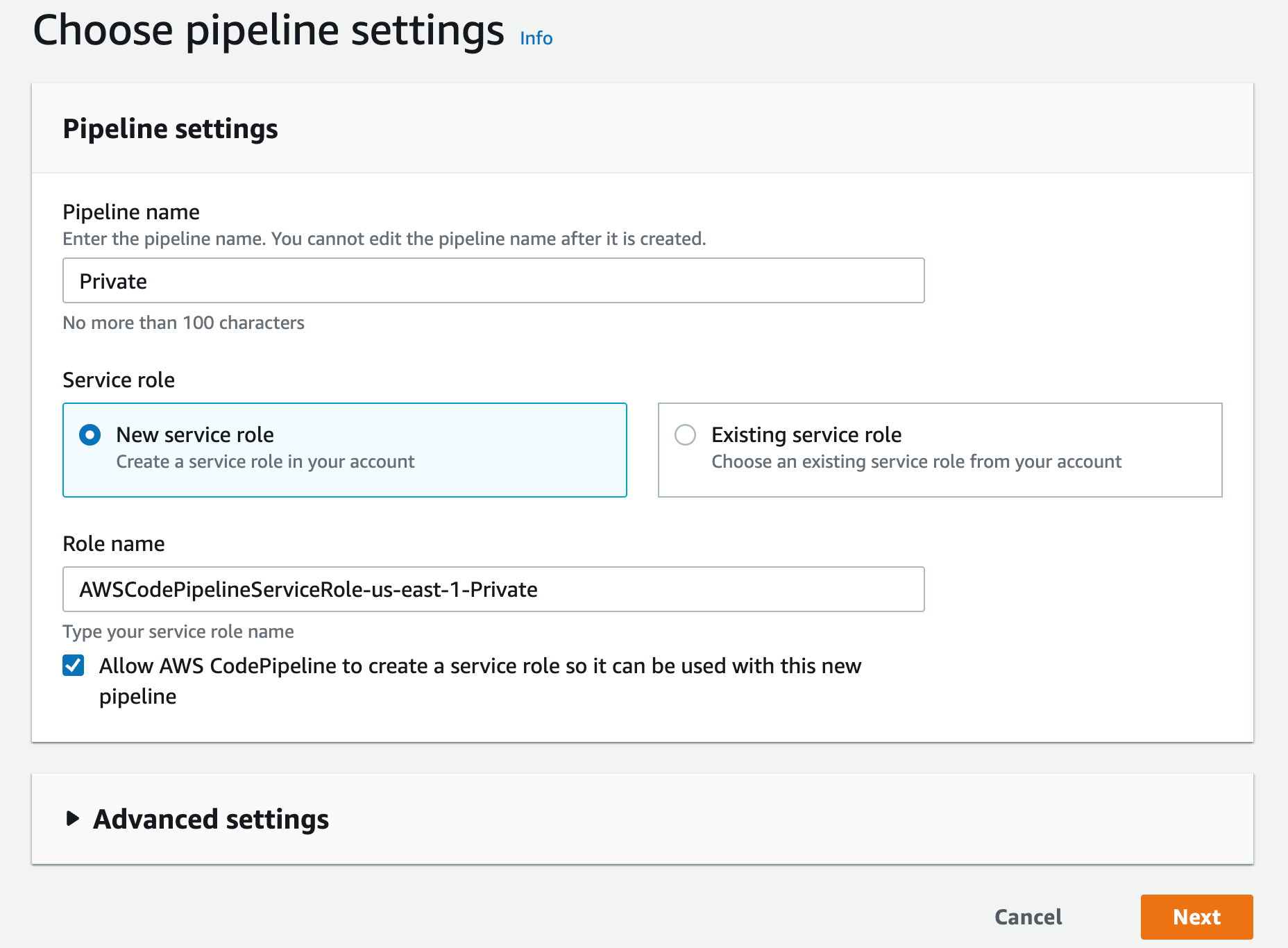
    1. Type a name, leave the Service role as “New service role” and click next
Figure 10. Screenshot: Choose pipeline setting page with pipeline name "Private".

Figure 10. Screenshot: Choose pipeline setting page with pipeline name “Private”.

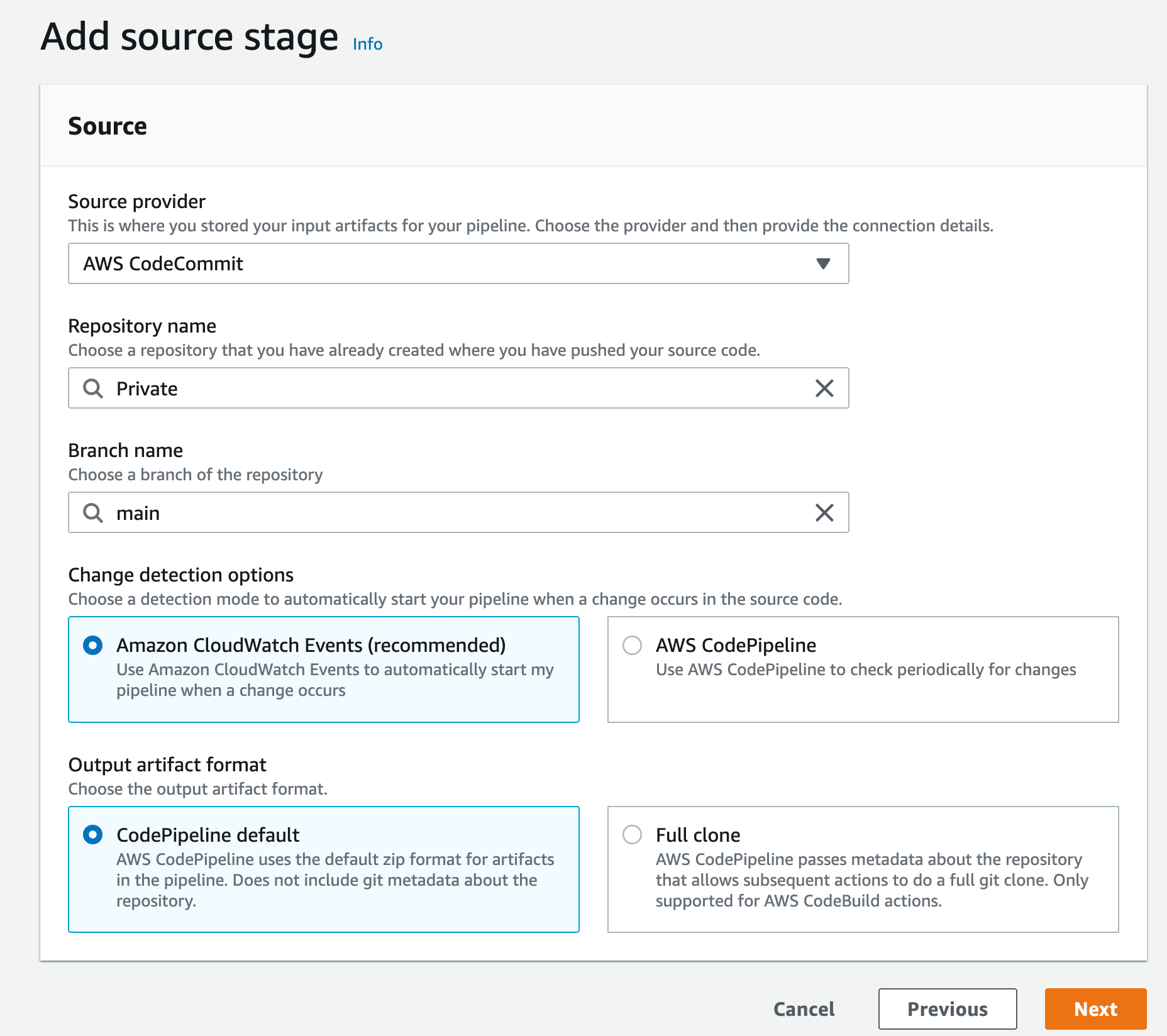
    1. Select AWS CodeCommit as your Source provider
    2. Then choose the CodeCommit repository you created earlier and for branch select main then click Next
Figure 11. Screenshot: Create pipeline add source stage.

Figure 11. Screenshot: Create pipeline add source stage.

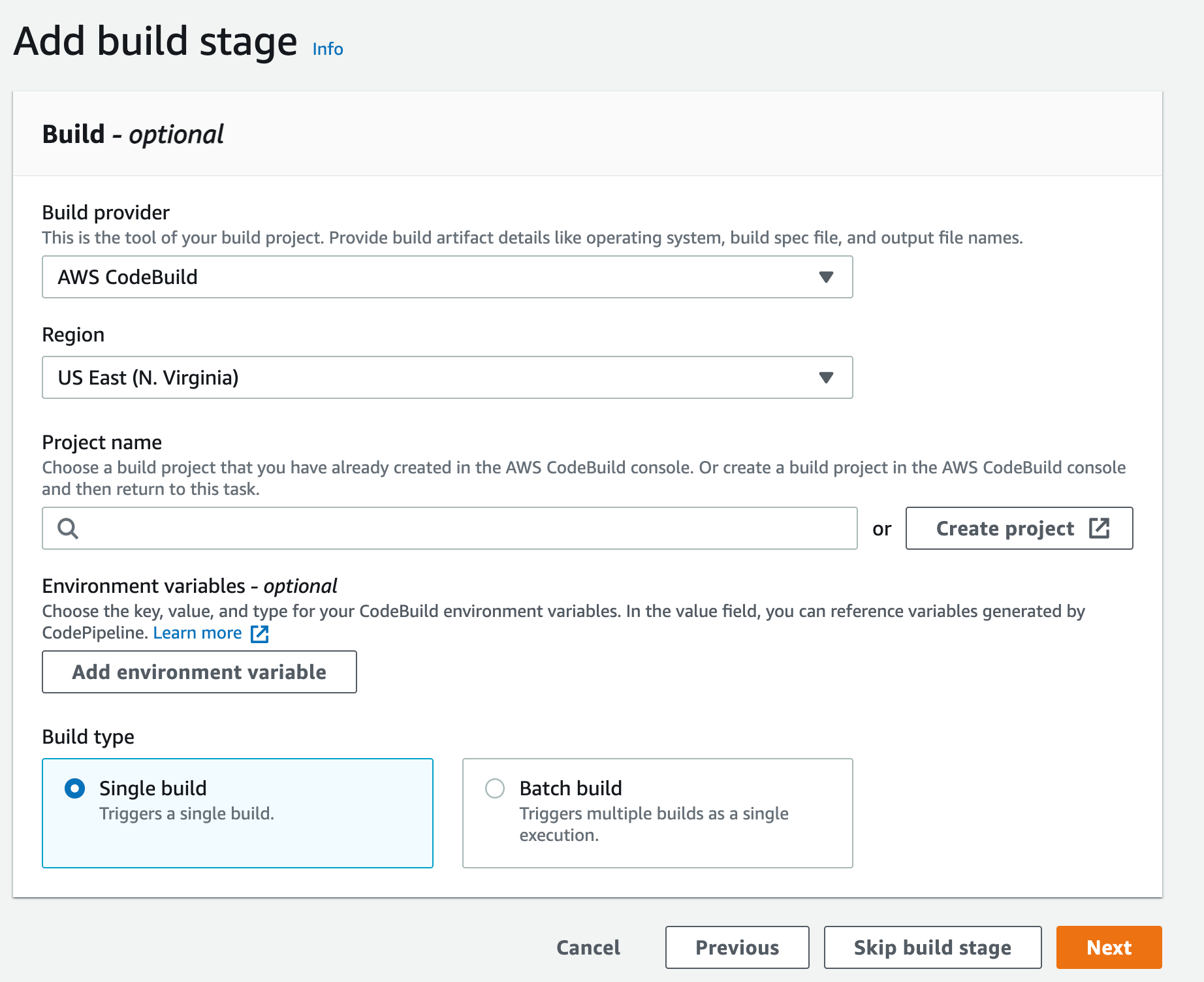
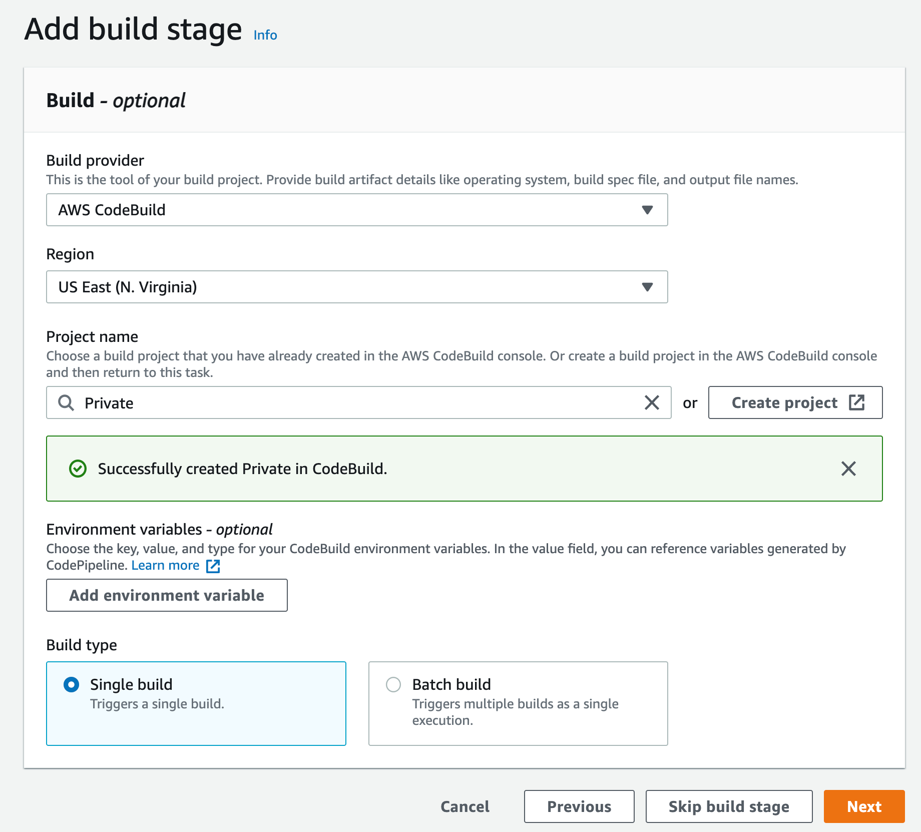
    1. For the Build Stage, Choose AWS CodeBuild as the build provider, then click Create Project
Figure 12. Screenshot: Create pipeline add build stage.

Figure 12. Screenshot: Create pipeline add build stage.

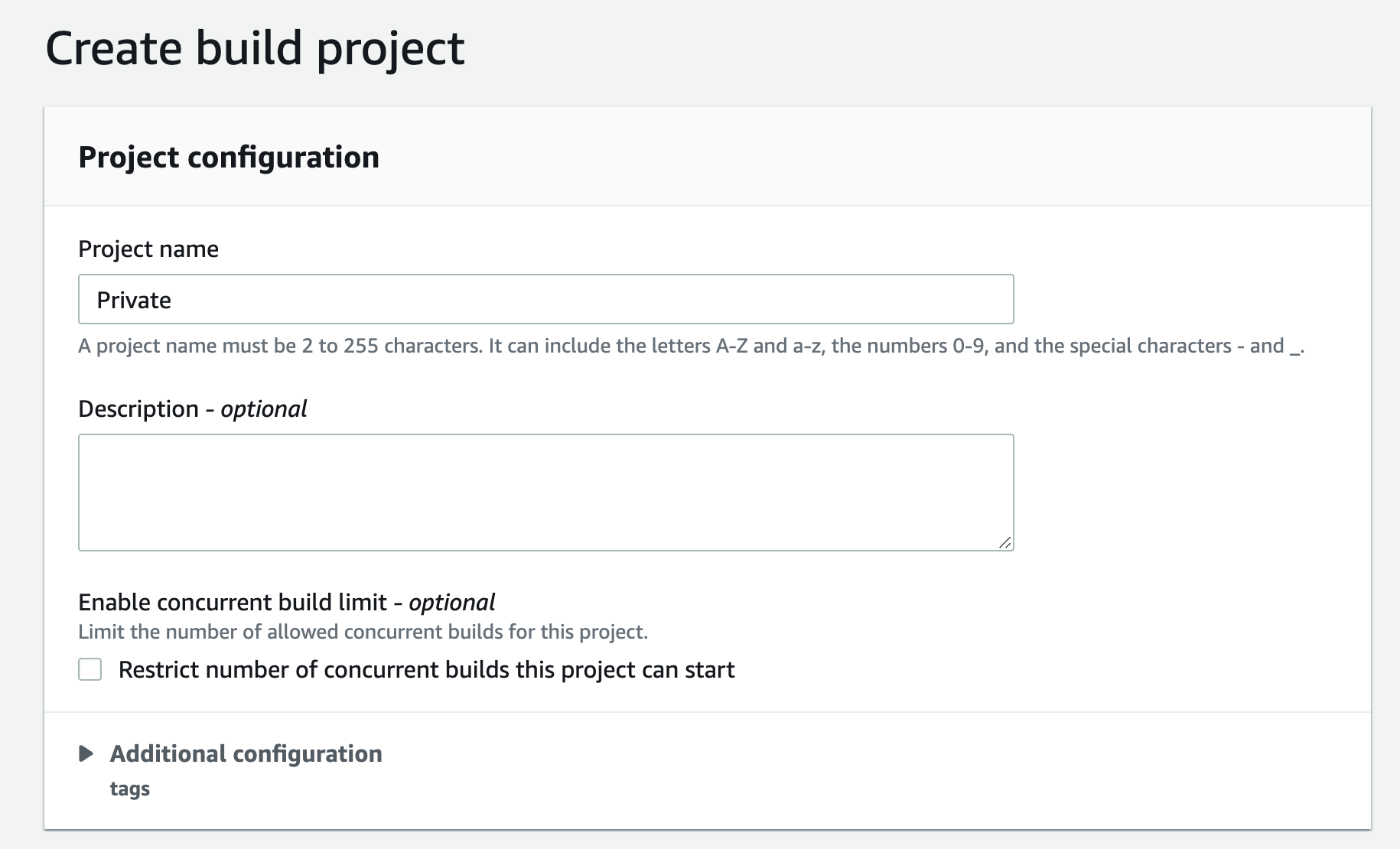
    1. This will open new window to create the new Project, Give this project a name
Figure 13. Screenshot: Create pipeline create build project window.

Figure 13. Screenshot: Create pipeline create build project window.

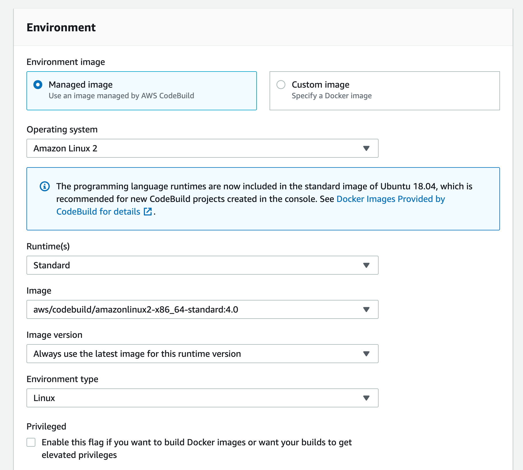
    1.  Scroll down to the Environment section: select pick Managed image,
    2. For Operating system select “Amazon Linux 2”,
    3. Runtime “Standard” and
    4. For Image select the aws/codebuild/amazonlinux2-x86+64-standard:4.0
      For the Image version: Always use the latest image for this runtime version
    5. Select Linux for the Environment type
    6. Leave the Privileged option unchecked and set Service Role to “New service role”
Figure 14. Screenshot: Create pipeline create build project, setting up environment window.

Figure 14. Screenshot: Create pipeline create build project, setting up environment window.

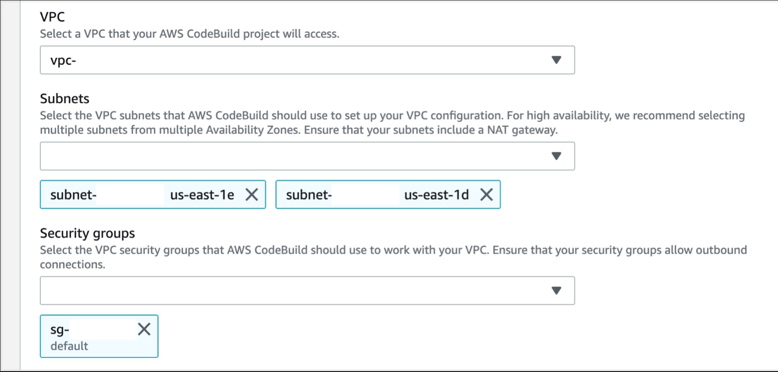
    1. Expand Additional configurations and scroll down to the VPC section, select the desired VPC, your Subnets (we recommend selecting multiple AZs, to ensure high availability), and Security Group (the security group rules must allow resources that will use the VPC endpoint to communicate with the AWS service to communicate with the endpoint network interface, default VPC security group will be used here as an example)
Figure 15. Screenshot: Create pipeline create build project networking window.

Figure 15. Screenshot: Create pipeline create build project networking window.

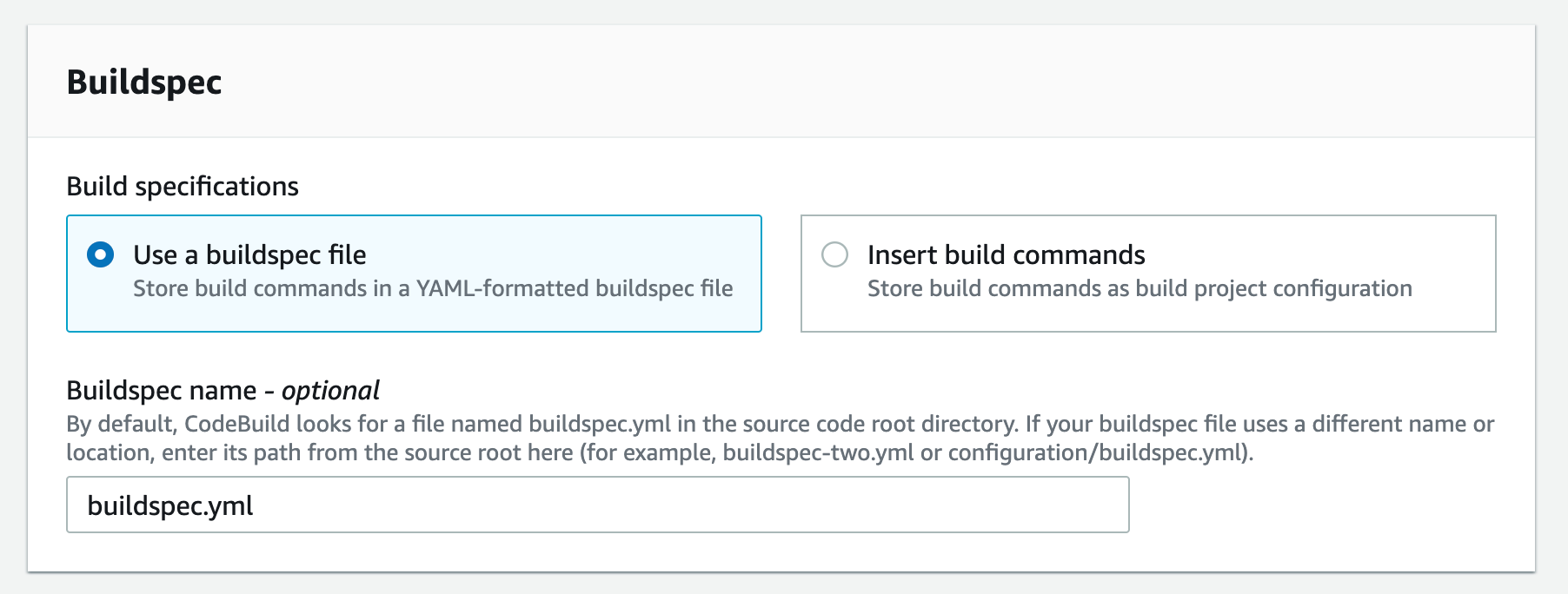
    1. Scroll down to the Buildspec and select “Use a buildspec file” and type “buildspec.yml” for the Buildspec name
Figure 16. Screenshot: Create pipeline create build project buildspec window.

Figure 16. Screenshot: Create pipeline create build project buildspec window.

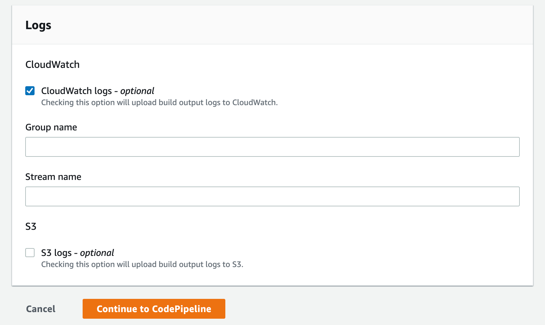
    1. Select the CloudWatch logs option you can leave the group name and stream empty this will let the service use the default values and click Continue to CodePipeline
Figure 17. Screenshot: Create pipeline create build project logs window.

Figure 17. Screenshot: Create pipeline create build project logs window.

    1. This will create the new CodeBuild Project, update the CodePipeline page, now you can click Next
Figure 18. Screenshot: Create pipeline add build stage window.

Figure 18. Screenshot: Create pipeline add build stage window.

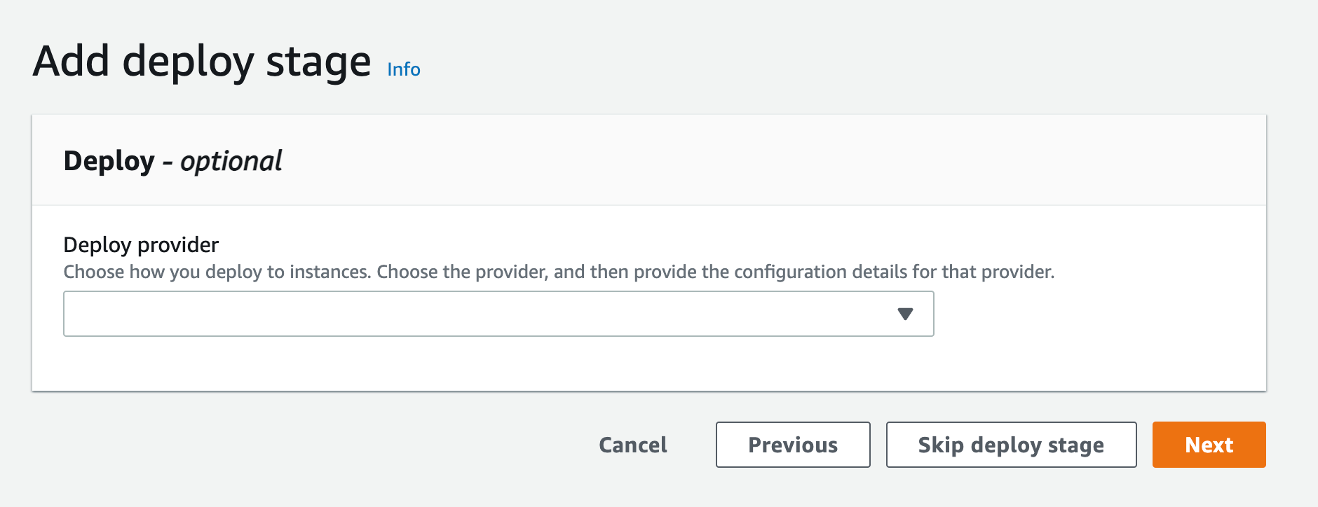
    1.  Since we are not deploying this to any environment, you can skip the deploy stage and click “Skip deploy stage”

Figure 19. Screenshot: Create pipeline add deploy stage.

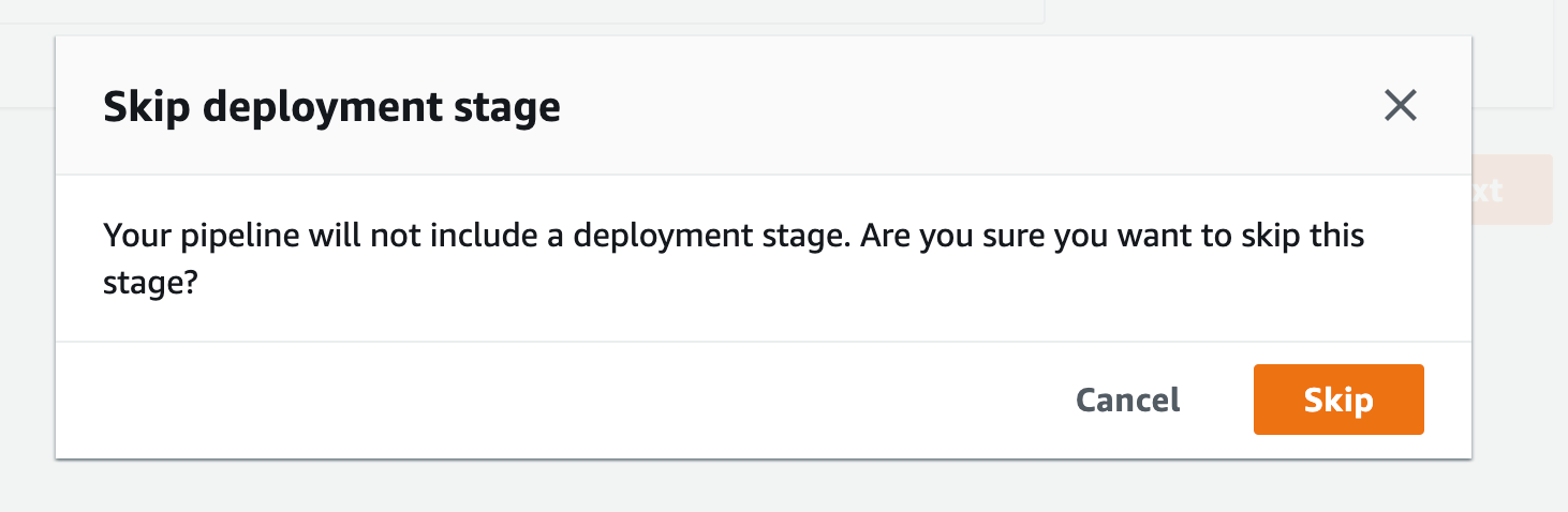
Figure 20. Screenshot: Create pipeline skip deployment stage confirmation.

Figure 20. Screenshot: Create pipeline skip deployment stage confirmation.

    1. After you get the popup click skip again you’ll see the review page, scroll all the way down and click Create Pipeline
  1. Create a VPC endpoint for Amazon CloudWatch Logs. This will enable CodeBuild to send execution logs to CloudWatch:
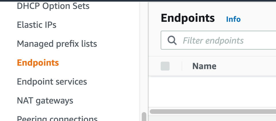
    1. Navigate to your VPC console, and from the navigation menu on the left select “Endpoints”.
Figure 21. Screenshot: VPC endpoint.

Figure 21. Screenshot: VPC endpoint.

    1.  click Create endpoint Button.
Figure 22. Screenshot: Create endpoint.

Figure 22. Screenshot: Create endpoint.

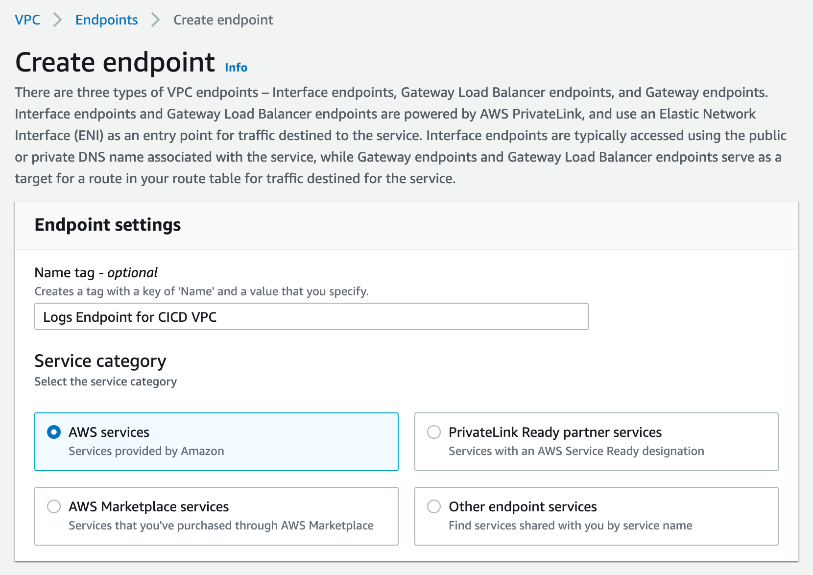
    1. For service Category, select “AWS Services”. You can set a name for the new endpoint, and make sure to use something descriptive.
Figure 23. Screenshot: Create endpoint page.

Figure 23. Screenshot: Create endpoint page.

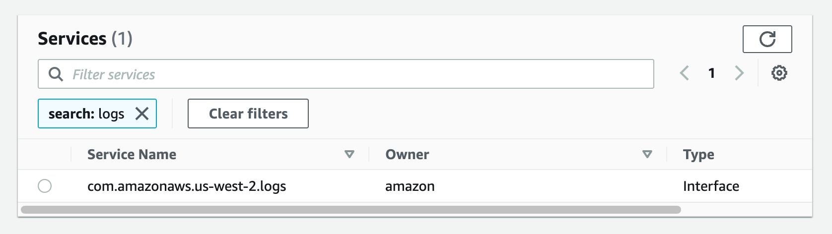
    1. From the list of services, search for the endpoint by typing logs in the search bar and selecting the one with com.amazonaws.us-west-2.logs.
      This walkthrough can be done in any region that supports the services. I am going to be using us-west-2, please select the appropriate region for your workload.
Figure 24. Screenshot: create endpoint select services with com.amazonaws.us-west-2.logs selected.

Figure 24. Screenshot: create endpoint select services with com.amazonaws.us-west-2.logs selected.

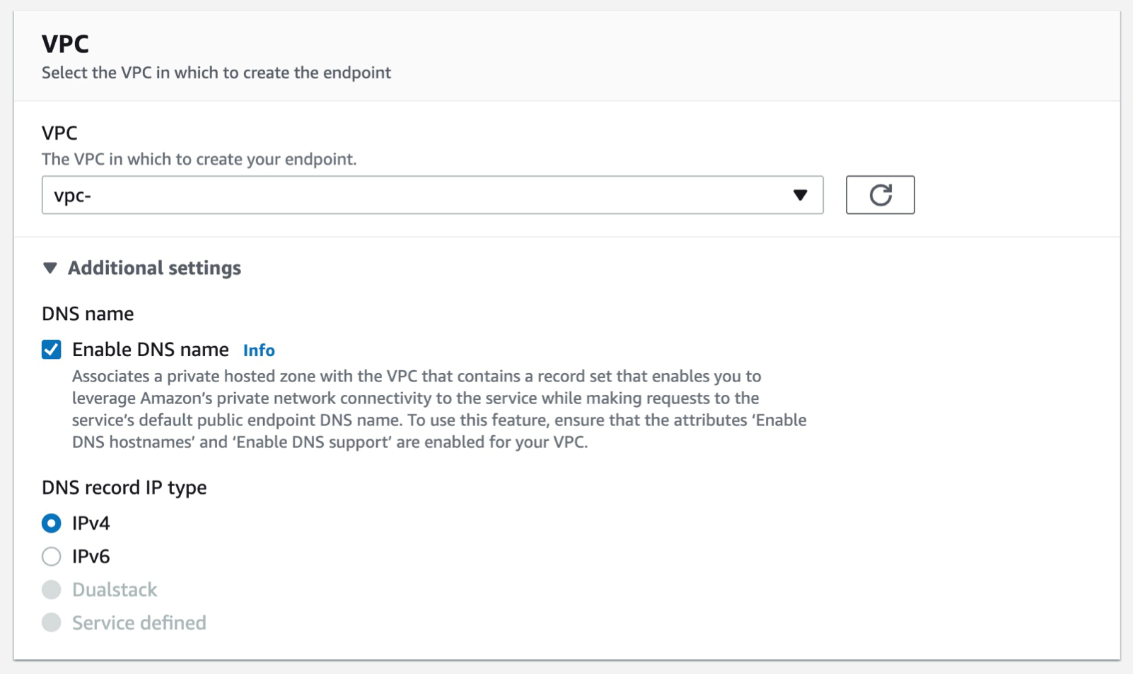
    1. Select the VPC that you want the endpoint to be associated with, and make sure that the Enable DNS name option is checked under additional settings.
Figure 25. Screenshot: create endpoint VPC setting shows VPC selected.

Figure 25. Screenshot: create endpoint VPC setting shows VPC selected.

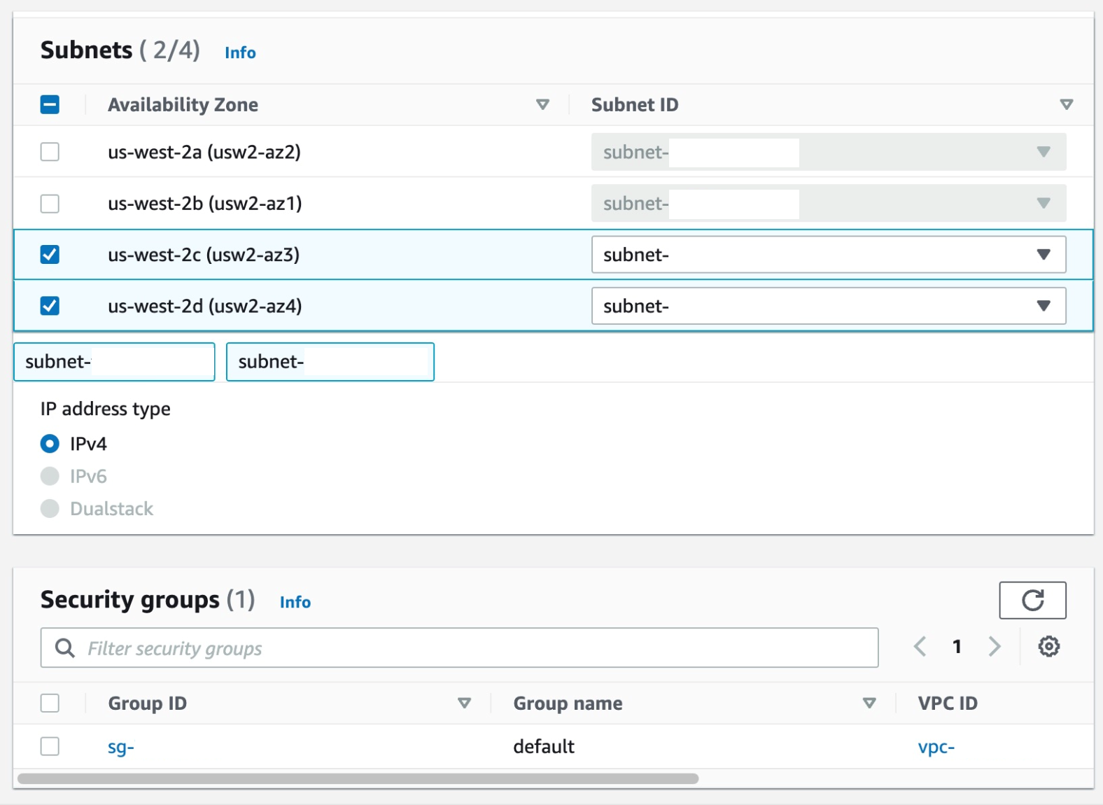
    1. Select the Subnets where you want the endpoint to be associated, and you can leave the security group as default and the policy as empty.
Figure 26. Screenshot: create endpoint subnet setting shows 2 subnet selected and default security group selected.

Figure 26. Screenshot: create endpoint subnet setting shows 2 subnet selected and default security group selected.

    1. Select Create Endpoint.
Figure 27. Screenshot: create endpoint button.

Figure 27. Screenshot: create endpoint button.

  1. Create a VPC endpoint for CodeArtifact. At the time of writing this article, CodeArifact has two endpoints: one is for API operations like service level operations and authentication, and the other is for using the service such as getting modules for our code. We’ll need both endpoints to automate working with CodeArtifact. Therefore, we’ll create both endpoints with DNS enabled.

In addition, we’ll need AWS Security Token Service (AWS STS) endpoint for get-caller-identity API call:

Follow steps a-c from the steps that were used from the creating the Logs endpoint above.

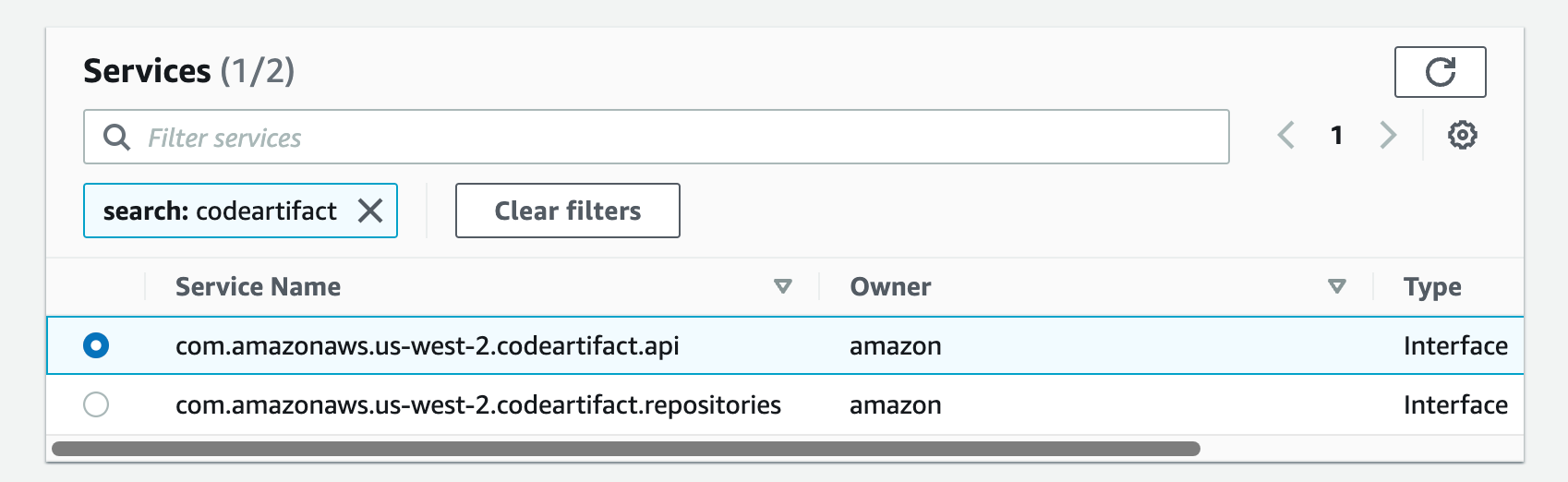
a. From the list of services, you can search for the endpoint by typing codeartifact in the search bar and selecting the one with com.amazonaws.us-west-2.codeartifact.api.

Figure 28. Screenshot: create endpoint select services with com.amazonaws.us-west-2.codeartifact.api selected.

Figure 28. Screenshot: create endpoint select services with com.amazonaws.us-west-2.codeartifact.api selected.

Follow steps e-g from Part 4.

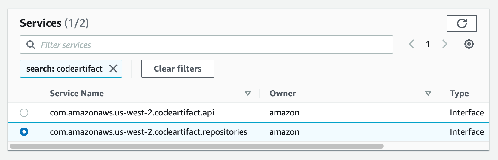
Then, repeat the same for com.amazon.aws.us-west-2.codeartifact.repositories service.

Figure 29. Screenshot: create endpoint select services with com.amazonaws.us-west-2.codeartifact.api selected.

Figure 29. Screenshot: create endpoint select services with com.amazonaws.us-west-2.codeartifact.api selected.

  1. Enable a VPC endpoint for AWS STS:

Follow steps a-c from Part 4

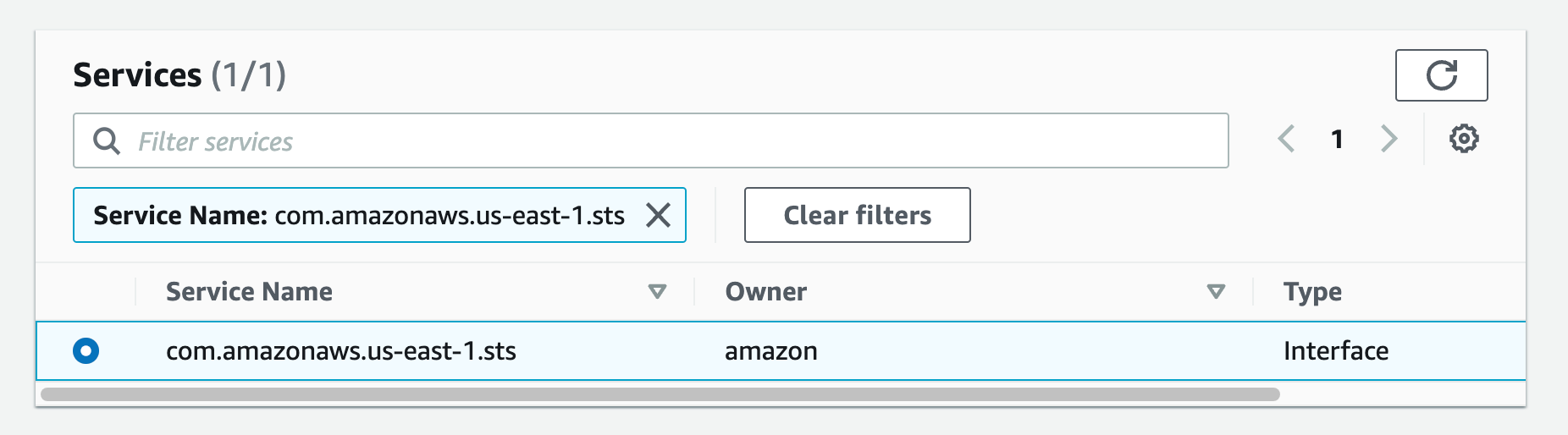
a. From the list of services you can search for the endpoint by typing sts in the search bar and selecting the one with com.amazonaws.us-west-2.sts.

Figure 30.Screenshot: create endpoint select services with com.amazon.aws.us-west-2.codeartifact.repositories selected.

Figure 30.Screenshot: create endpoint select services with com.amazon.aws.us-west-2.codeartifact.repositories selected.

Then follow steps e-g from Part 4.

  1. Create a VPC endpoint for S3:

Follow steps a-c from Part 4

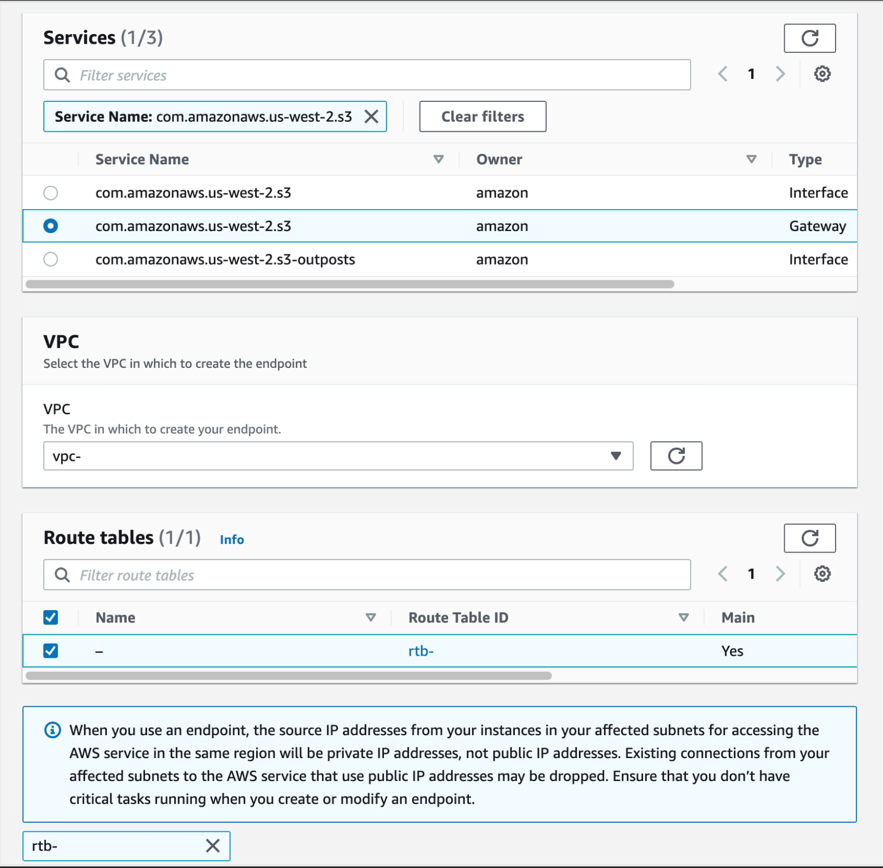
a. From the list of services you can search for the endpoint by typing sts in the search bar and selecting the one with com.amazonaws.us-west-2.s3, select the one with type of Gateway

Then select your VPC, and select the route tables for your subnets, this will auto update the route table with the new S3 endpoint.

Figure 31. Screenshot: create endpoint select services with com.amazonaws.us-west-2.s3 selected.

Figure 31. Screenshot: create endpoint select services with com.amazonaws.us-west-2.s3 selected.

  1. Now we have all of the endpoints set. The last step is to update your pipeline to point at the CodeArtifact repository when pulling your code dependencies. I’ll use CodeBuild buildspec.yml as an example here.

Make sure that your CodeBuild AWS Identity and Access Management (IAM) role has the permissions to perform STS and CodeArtifact actions.

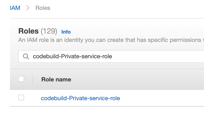
Navigate to IAM console and click Roles from the left navigation menu, then search for your IAM role name, in our case since we selected “New service role” option in step 2.k was created with the name “codebuild-Private-service-role” (codebuild-<BUILD PROJECT NAME>-service-role)

Figure 32. Screenshot: IAM roles with codebuild-Private-service-role role shown in search.

Figure 32. Screenshot: IAM roles with codebuild-Private-service-role role shown in search.

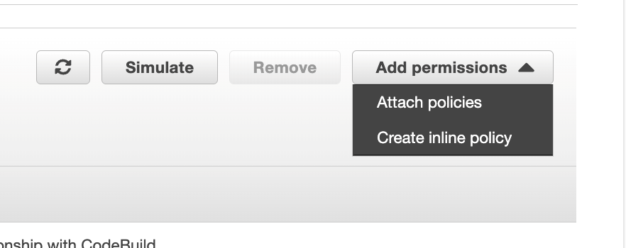
From the Add permissions menu, click on Create inline policy

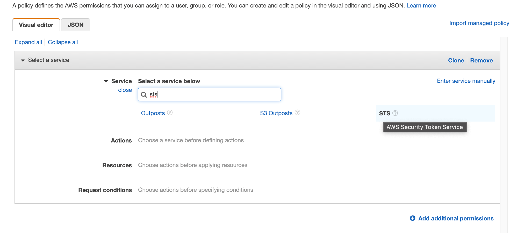
Search for STS in the services then select STS

Figure 34. Screenshot: IAM visual editor with sts shown in search.

Figure 34. Screenshot: IAM visual editor with sts shown in search.

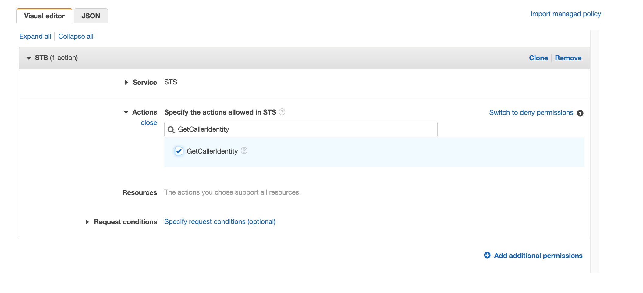
Search for “GetCallerIdentity” and select the action

Figure 35. Screenshot: IAM visual editor with GetCallerIdentity in search and action selected.

Figure 35. Screenshot: IAM visual editor with GetCallerIdentity in search and action selected.

Repeat the same with “GetServiceBearerToken”

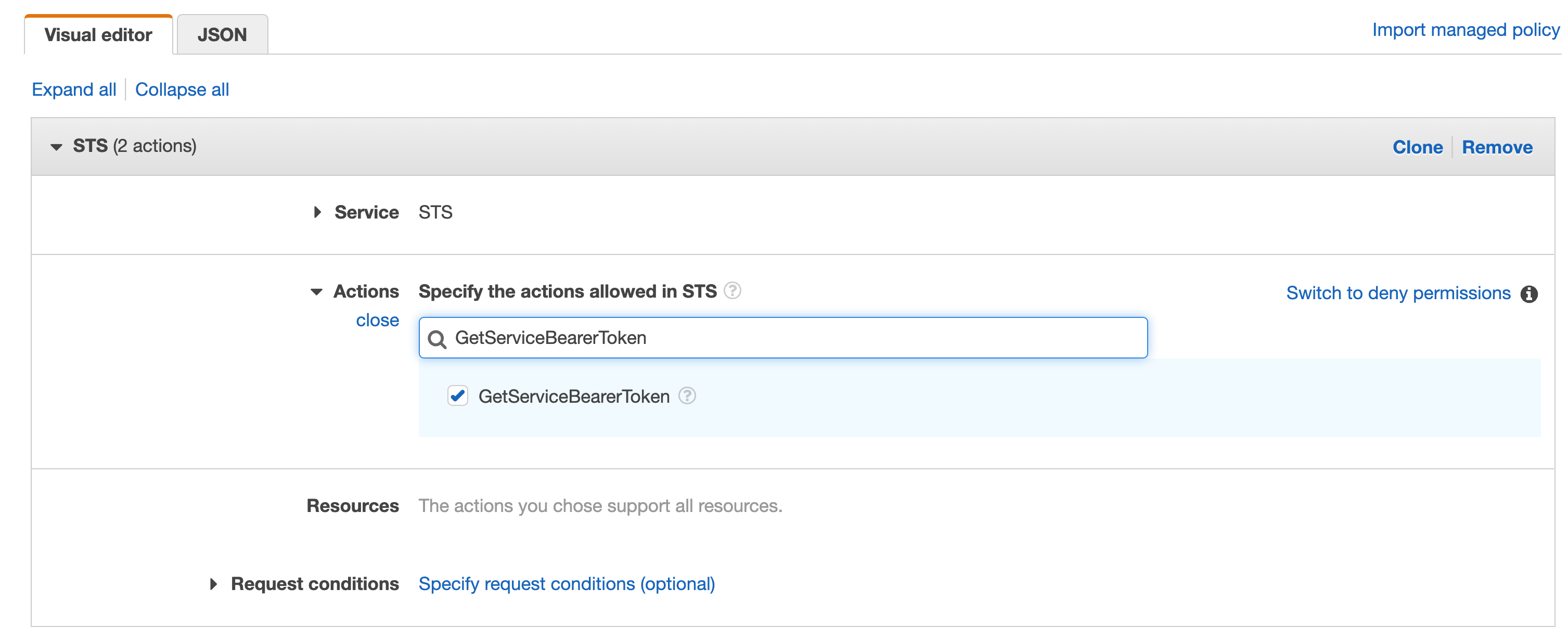
Figure 36. Screenshot: IAM visual editor with GetServiceBearerToken in search and action selected.

Figure 36. Screenshot: IAM visual editor with GetServiceBearerToken in search and action selected.

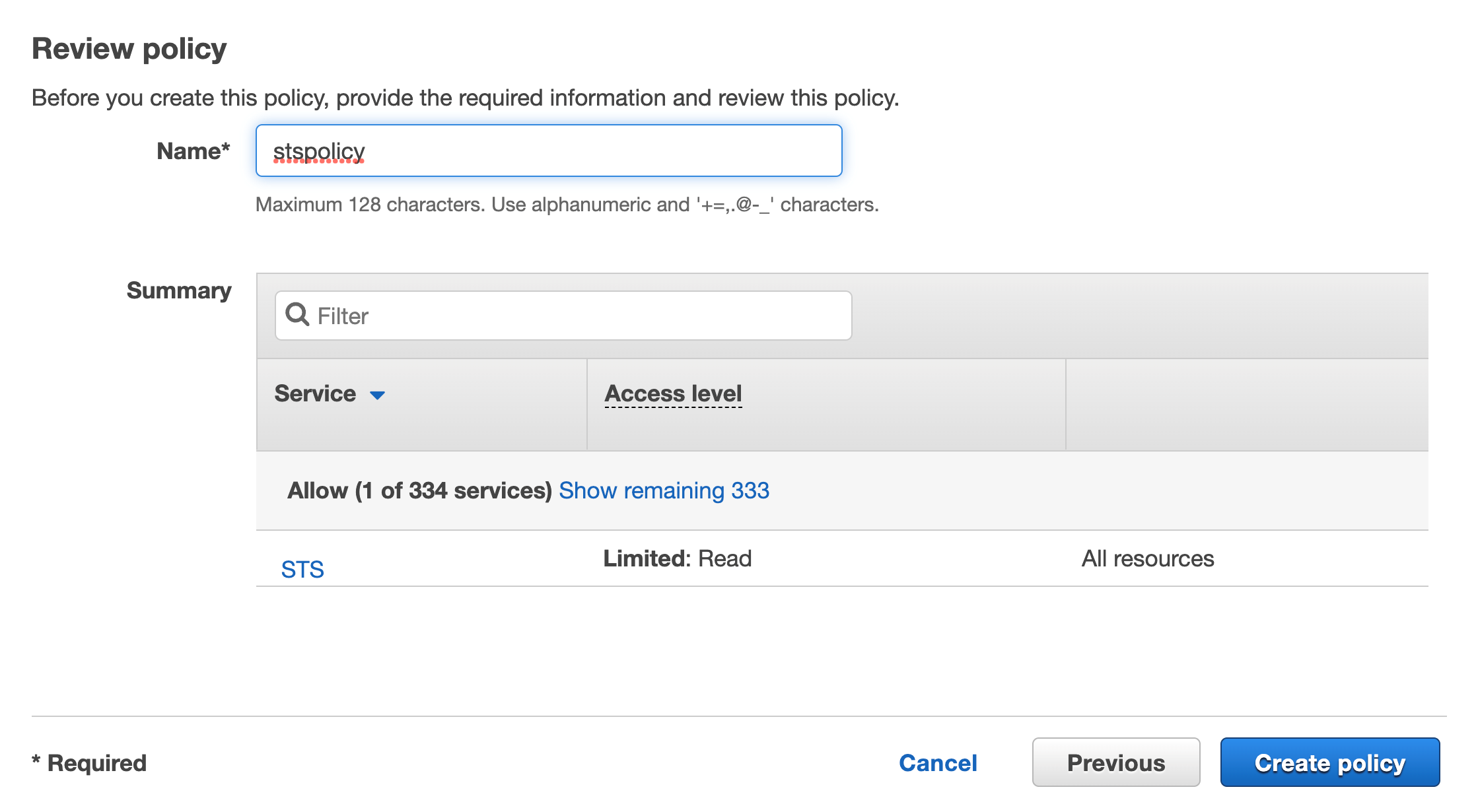
Click on Review, add a name then click on Create policy

Figure 37. Screenshot: Review page and Create policy button.

Figure 37. Screenshot: Review page and Create policy button.

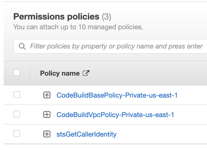
You should see the new inline policy added to the list

Figure 38. Screenshot: shows the new in-line policy in the list.

Figure 38. Screenshot: shows the new in-line policy in the list.

For CodeArtifact actions we will do the same on that role, click on Create inline policy

Figure 39. Screenshot: attach policies.

Figure 39. Screenshot: attach policies.

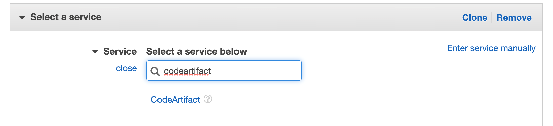
Search for CodeArtifact in the services then select CodeArtifact

Figure 40. Screenshot: select service with CodeArtifact in search.

Figure 40. Screenshot: select service with CodeArtifact in search.

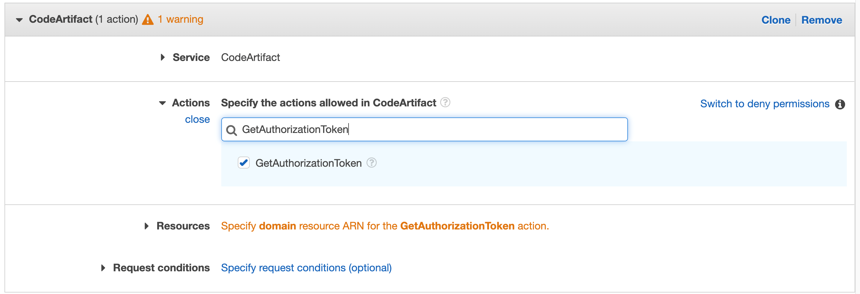
Search for “GetAuthorizationToken” in actions and select that action in the check box

Figure 41. CodeArtifact: with GetAuthorizationToken in search.

Figure 41. CodeArtifact: with GetAuthorizationToken in search.

Repeat for “GetRepositoryEndpoint” and “ReadFromRepository”

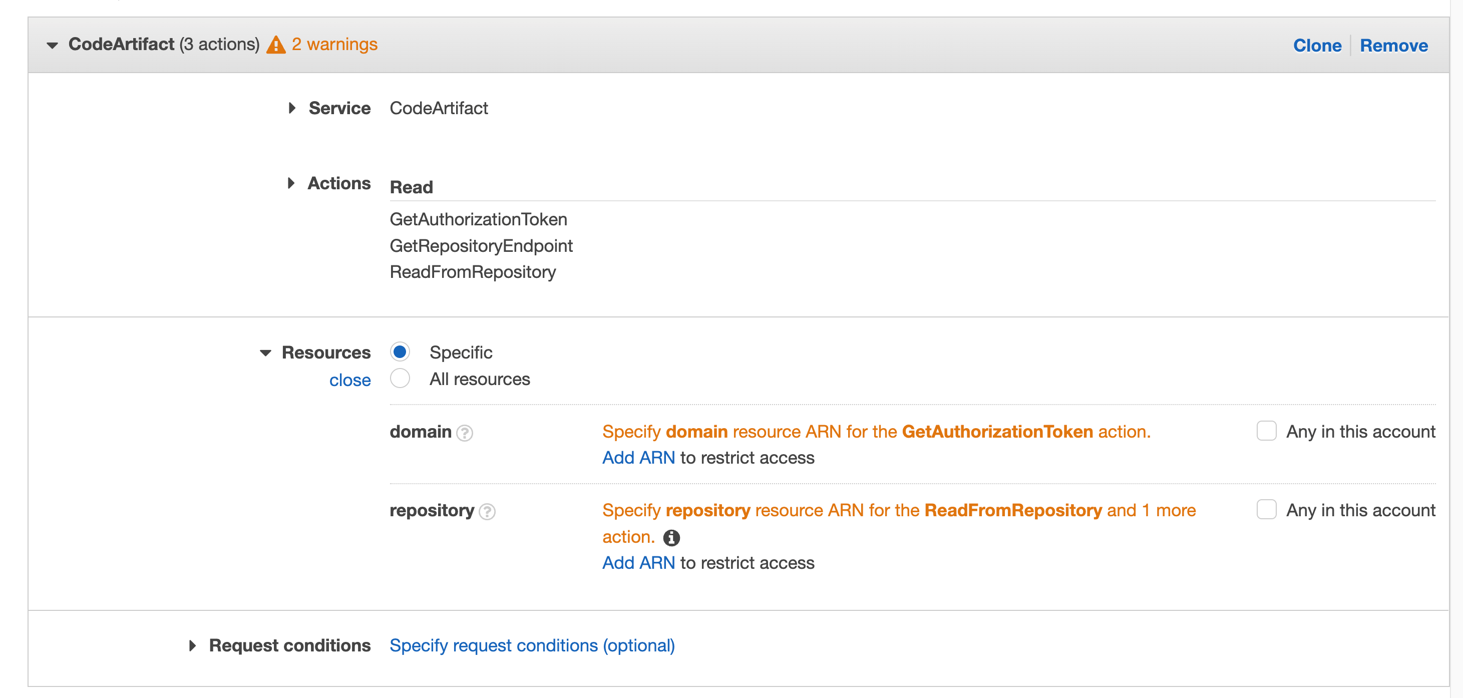
Click on Resources to fix the 2 warnings, then click on Add ARN on the first one “Specify domain resource ARN for the GetAuthorizationToken action.”

Figure 42. Screenshot: with all selected filed and 2 warnings.

Figure 42. Screenshot: with all selected filed and 2 warnings.

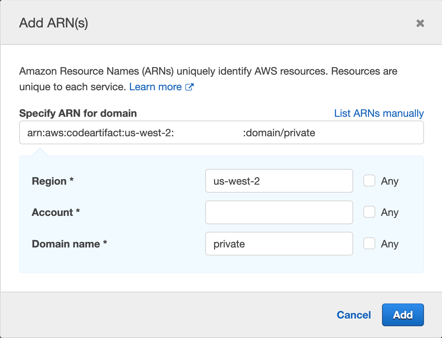
You’ll get a pop up with fields for Region, Account and Domain name, enter your region, your account number, and the domain name, we used “private” when we created our domain earlier.

Figure 43. Screenshot: Add ARN page.

Figure 43. Screenshot: Add ARN page.

Then click Add

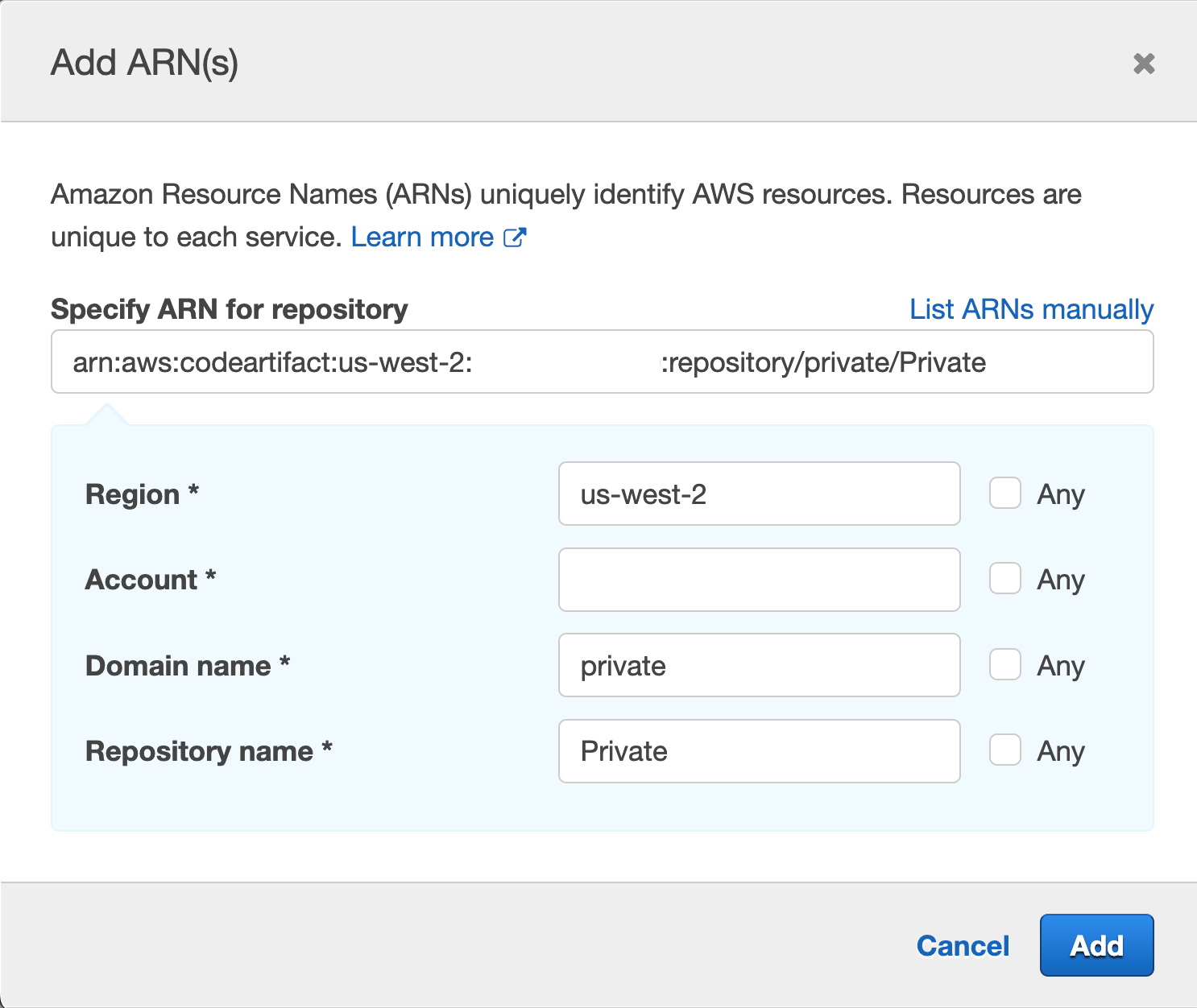
Repeat the same process for “Specify repository resource ARN for the ReadFromRepository and 1 more”, and this time we will provide Region, Account ID, Domain name and Repository name, we used “Private” for the repository we created earlier and “private” for domain

Figure 44. Screenshot: add ARN page.

Figure 44. Screenshot: add ARN page.

Note it is best practice to specify the resource we are targeting, we can use the checkbox for “Any” but we want to narrow the scope of our IAM role best we can.

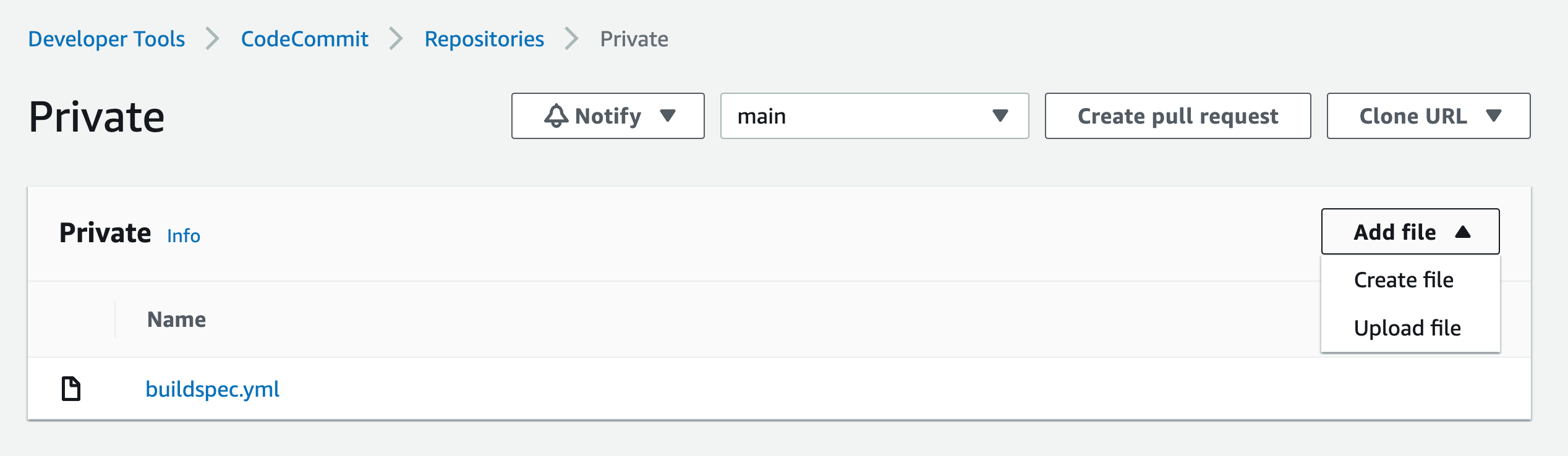
  1. Navigate to CodeCommit then click on the repo you created earlier in step1
Figure 45. Screenshot: CodeCommit repo.

Figure 45. Screenshot: CodeCommit repo.

Click on Add file dropdown, then Create file button

Paste the following in the editor space:

{
  "dependencies": {
    "mathjs": "^11.2.0"
  }
}

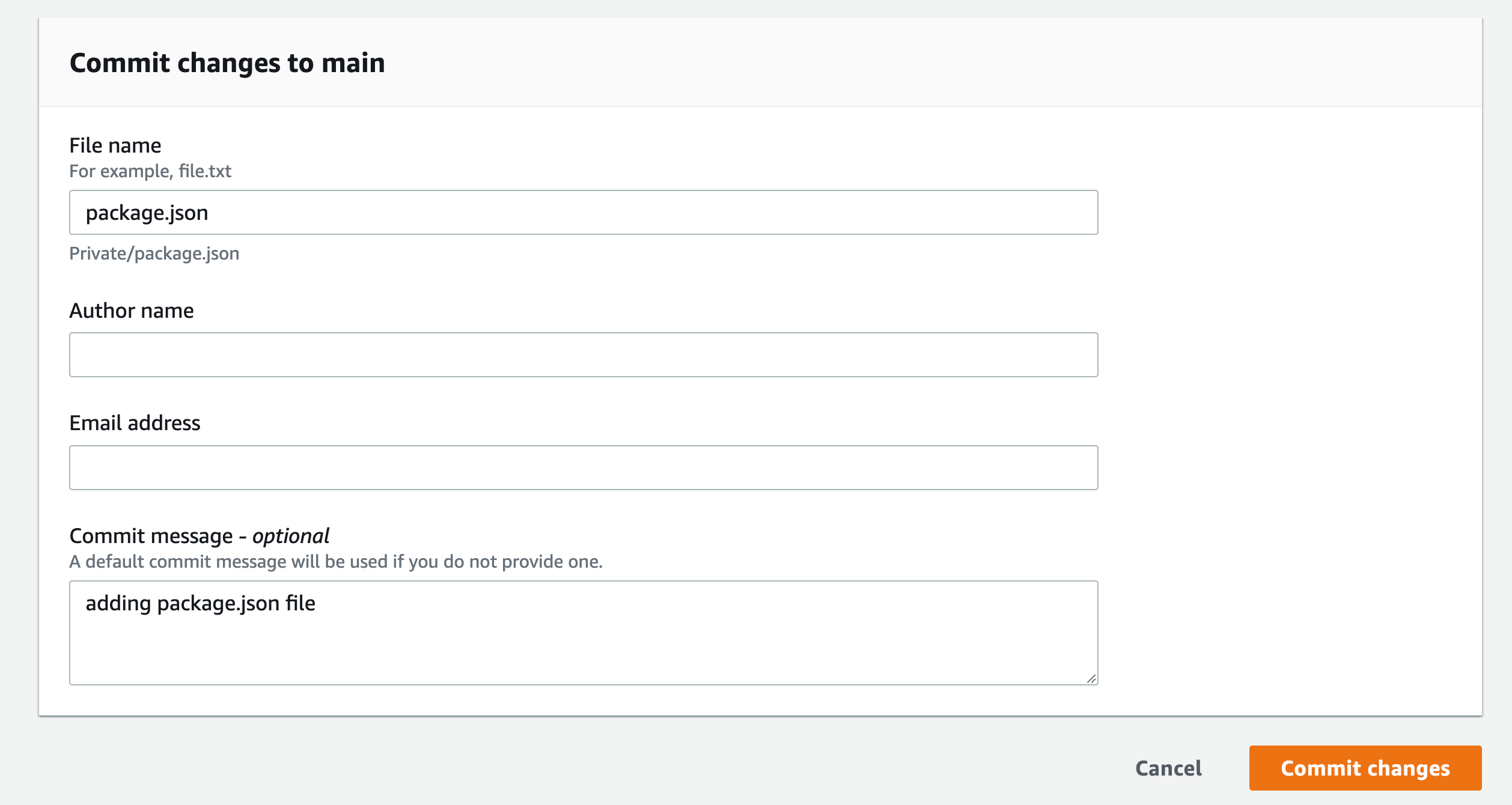
Name the file “package.json”

Add your name and email, and optional commit message

Repeat this process for “index.js” and paste the following in the editor space:

const { sqrt } = require('mathjs')
console.log(sqrt(49).toString())

Figure 46. Screenshot: CodeCommit Commit changes button.

Figure 46. Screenshot: CodeCommit Commit changes button.


This will force the pipeline to kick off and start building the application

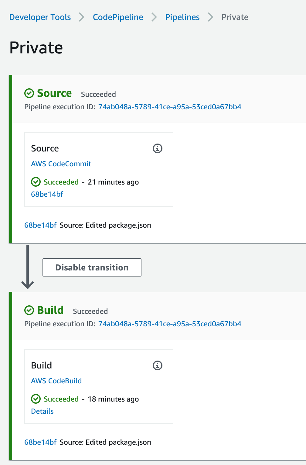
Figure 47. Screenshot: CodePipeline.

Figure 47. Screenshot: CodePipeline.

This is a very simple application that gets the square root of 49 and log it to the screen, if you click on the Details link from the pipeline build stage, you’ll see the output of running the NodeJS application, the logs are stored in CloudWatch and you can navigate there by clicking on the link the View entire log “Showing the last xx lines of the build log. View entire log”

Figure 48. Screenshot: Showing the last 54 lines of the build log. View entire log.

Figure 48. Screenshot: Showing the last 54 lines of the build log. View entire log.

We used npm example in the buildspec.yml above, Similar setup will be used for pip and twine,

For Maven, Gradle, and NuGet, you must set Environment variables and change your settings.xml and build.gradle, as well as install the plugin for your IDE. For more information, see here.

Cleanup

Navigate to VPC endpoint from the AWS console and delete the endpoints that you created.

Navigate to CodePipeline and delete the Pipeline you created.

Navigate to CodeBuild and delete the Build Project created.

Navigate to CodeCommit and delete the Repository you created.

Navigate to CodeArtifact and delete the Repository and the domain you created.

Navigate to IAM and delete the Roles created:

For CodeBuild: codebuild-<Build Project Name>-service-role

For CodePipeline: AWSCodePipelineServiceRole-<Region>-<Project Name>

Conclusion

In this post, we deployed a full CI/CD pipeline with CodePipeline orchestrating CodeBuild to build and test a small NodeJS application, using CodeArtifact to download the application code dependencies. All without going to the public internet and maintaining the logs in CloudWatch.

About the author:

MJ Kubba

MJ Kubba is a Solutions Architect who enjoys working with public sector customers to build solutions that meet their business needs. MJ has over 15 years of experience designing and implementing software solutions. He has a keen passion for DevOps and cultural transformation.

Team Collaboration with Amazon CodeCatalyst

Post Syndicated from original https://aws.amazon.com/blogs/devops/team-collaboration-with-amazon-codecatalyst/

Amazon CodeCatalyst enables teams to collaborate on features, tasks, bugs, and any other work involved when building software. CodeCatalyst was announced at re:Invent 2022 and is currently in preview.

Introduction:

In a prior post in this series, Using Workflows to Build, Test, and Deploy with Amazon CodeCatalyst, I discussed reading The Unicorn Project, by Gene Kim, and how the main character, Maxine, struggles with a complicated software development lifecycle (SLDC) after joining a new team. Some of the challenges she encounters include:

  • Continually delivering high-quality updates is complicated and slow
  • Collaborating efficiently with others is challenging
  • Managing application environments is increasingly complex
  • Setting up a new project is a time-consuming chore

In this post, I will focus on the second bullet, and how CodeCatalyst helps you collaborate from anywhere with anyone.

Prerequisites

If you would like to follow along with this walkthrough, you will need to:

Walkthrough

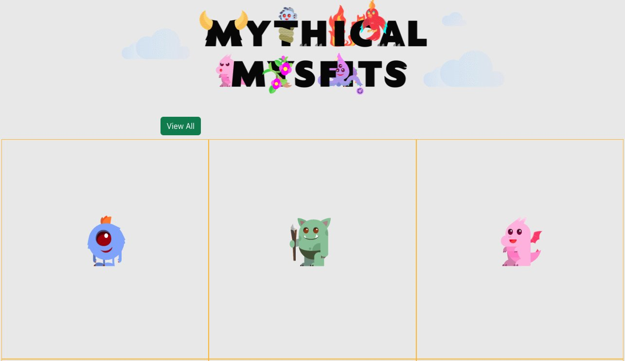
Similar to the prior post, I am going to use the Modern Three-tier Web Application blueprint in this walkthrough. A CodeCatalyst blueprint provides a template for a new project. If you would like to follow along, you can launch the blueprint as described in Creating a project in Amazon CodeCatalyst.  This will deploy the Mythical Mysfits sample application shown in the following image.

The Mythical Mysfits user interface showing header and three Mysfits

Figure 1. The Mythical Mysfits user interface showing header and three Mysfits

For this Walkthrough, let us assume that I need to make a simple change to the application. The legal department would like to add a footer that includes the text “© 2023 Demo Organization.” I will create an issue in CodeCatalyst to track this work and use CodeCatalyst to track the change throughout the entire Software Development Life Cycle (SDLC).

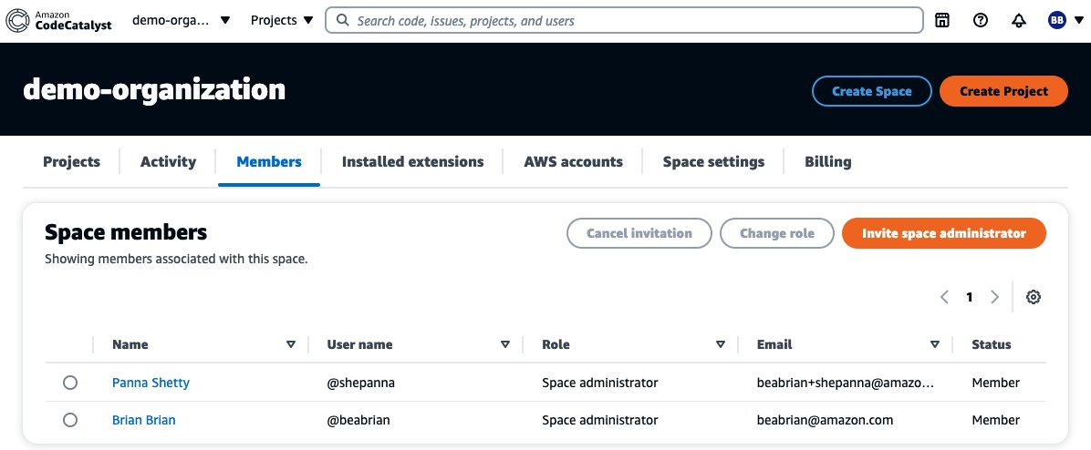
CodeCatalyst organizes projects into Spaces. A space represents your company, department, or group; and contains projects, members, and the associated cloud resources you create in CodeCatalyst. In this walkthrough, my Space currently includes two members, Brian Beach and Panna Shetty, as shown in the following screenshot.  Note that both users are administrators, but CodeCatalyst supports multiple roles. You can read more about roles in members of your space.

The space members configuration page showing two users

Figure 2. The space members configuration page showing two users

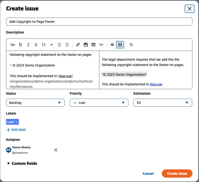
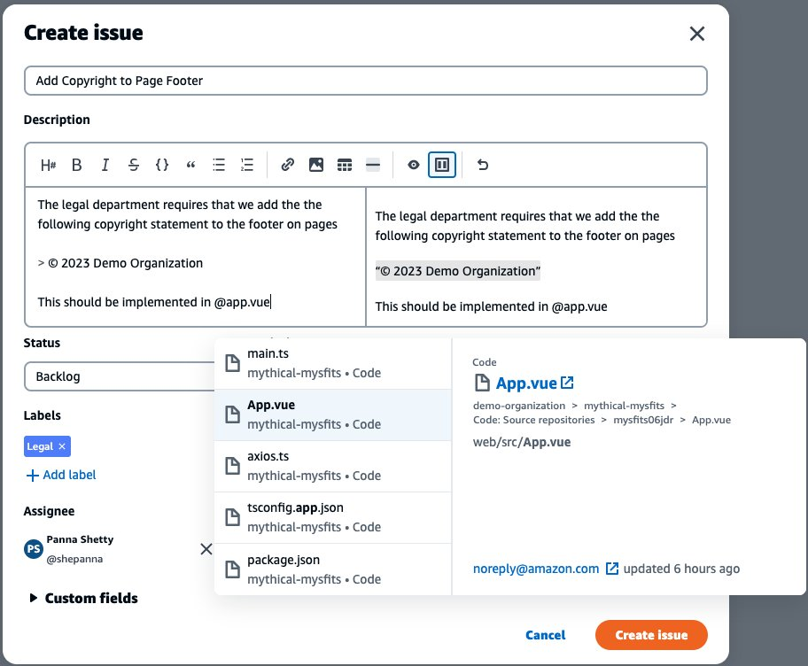
To begin, Brian creates a new issue to track the request from legal. He assigns the issue to Panna, but leaves it in the backlog for now. Note that CodeCatalyst supports multiple metadata fields to organize your work. This issue is not impacting users and is relatively simple to fix. Therefore, Brian has categorized it as low priority and estimated the effort as extra small (XS). Brian has also added a label, so all the requests from legal can be tracked together. Note that these metadata fields are customizable. You can read more in configuring issue settings.

Create issue dialog box with name, description and metadata

Figure 3. Create issue dialog box with name, description and metadata

CodeCatalyst supports rich markdown in the description field. You can read about this in Markdown tips and tricks. In the following screenshot, Brian types “@app.vue” which brings up an inline search for people, issues, and code to help Panna find the relevant bit of code that needs changing later.
Create issue dialog box with type-ahead overlay

Figure 4. Create issue dialog box with type-ahead overlay

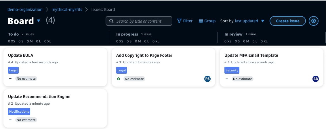
When Panna is ready to begin work on the new feature, she moves the issue from the “Backlog“ to ”In progress.“ CodeCatalyst allows users to manage their work using a Kanban style board. Panna can simply drag-and-drop issues on the board to move the issue from one state to another. Given the small team, Brian and Panna use a single board. However, CodeCatalyst allows you to create multiple views filtered by the metadata fields discussed earlier. For example, you might create a label called Sprint-001, and use that to create a board for the sprint.
Kanban board showing to do, in progress and in review columns

Figure 5. Kanban board showing to do, in progress and in review columns

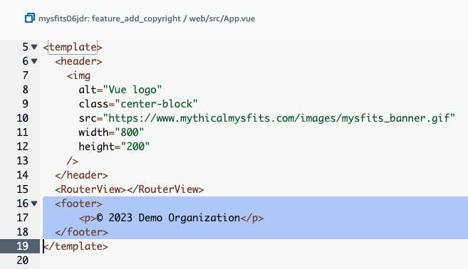
Panna creates a new branch for the change called feature_add_copyright and uses the link in the issue description to navigate to the source code repository. This change is so simple that she decides to edit the file in the browser and commits the change. Note that for more complex changes, CodeCatalyst supports Dev Environments. The next post in this series will be dedicated to Dev Environments. For now, you just need to know that a Dev Environment is a cloud-based development environment that you can use to quickly work on the code stored in the source repositories of your project.

Editor with new lines highlighted

Figure 6. Editor with new lines highlighted

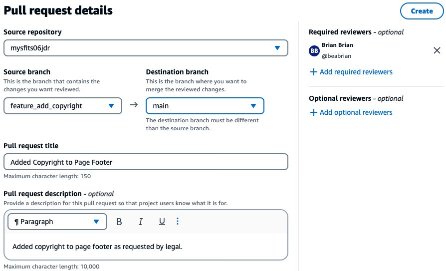
Panna also creates a pull request to merge the feature branch in to the main branch. She identifies Brian as a required reviewer. Panna then moves the issue to the “In review” column on the Kanban board so the rest of the team can track the progress. Once Brian reviews the change, he approves and merges the pull request.

Pull request details with title, description, and reviewed assigned

Figure 7. Pull request details with title, description, and reviewed assigned

When the pull request is merged, a workflow is configured to run automatically on code changes to build, test, and deploy the change. Note that Workflows were covered in the prior post in this series. Once the workflow is complete, Panna is notified in the team’s Slack channel. You can read more about notifications in working with notifications in CodeCatalyst. She verifies the change in production and moves the issue to the done column on the Kanban board.

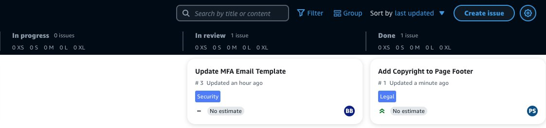
Kanban board showing in progress, in review, and done columns

Figure 8. Kanban board showing in progress, in review, and done columns

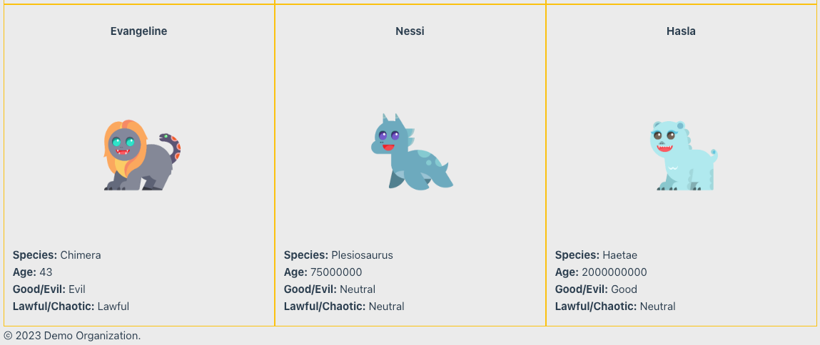
Once the deployment completes, you will see the footer added at the bottom of the page.

Figure 9. The Mythical Mysfits user interface showing footer and three Mysfits

At this point the issue is complete and you have seen how this small team collaborated to progress through the entire software development lifecycle (SDLC).

Cleanup

If you have been following along with this workflow, you should delete the resources you deployed so you do not continue to incur charges. First, delete the two stacks that CDK deployed using the AWS CloudFormation console in the AWS account you associated when you launched the blueprint. These stacks will have names like mysfitsXXXXXWebStack and mysfitsXXXXXAppStack. Second, delete the project from CodeCatalyst by navigating to Project settings and choosing Delete project.

Conclusion

In this post, you learned how CodeCatalyst can help you rapidly collaborate with other developers. I used issues to track feature and bugs, assigned code reviews, and managed pull requests. In future posts I will continue to discuss how CodeCatalyst can address the rest of the challenges Maxine encountered in The Unicorn Project.

About the authors:

Brian Beach

Brian Beach has over 20 years of experience as a Developer and Architect. He is currently a Principal Solutions Architect at Amazon Web Services. He holds a Computer Engineering degree from NYU Poly and an MBA from Rutgers Business School. He is the author of “Pro PowerShell for Amazon Web Services” from Apress. He is a regular author and has spoken at numerous events. Brian lives in North Carolina with his wife and three kids.

Panna Shetty

Panna Shetty is a Sr. Solutions Architect with Amazon Web Services (AWS), working with public sector customers. She enjoys helping customers architect and build scalable and
reliable modern applications using cloud-native technologies.

Secure CDK deployments with IAM permission boundaries

Post Syndicated from Brian Farnhill original https://aws.amazon.com/blogs/devops/secure-cdk-deployments-with-iam-permission-boundaries/

The AWS Cloud Development Kit (CDK) accelerates cloud development by allowing developers to use common programming languages when modelling their applications. To take advantage of this speed, developers need to operate in an environment where permissions and security controls don’t slow things down, and in a tightly controlled environment this is not always the case. Of particular concern is the scenario where a developer has permission to create AWS Identity and Access Management (IAM) entities (such as users or roles), as these could have permissions beyond that of the developer who created them, allowing for an escalation of privileges. This approach is typically controlled through the use of permission boundaries for IAM entities, and in this post you will learn how these boundaries can now be applied more effectively to CDK development – allowing developers to stay secure and move fast.

Time to read 10 minutes
Learning level Advanced (300)
Services used

AWS Cloud Development Kit (CDK)

AWS Identity and Access Management (IAM)

Applying custom permission boundaries to CDK deployments

When the CDK deploys a solution, it assumes a AWS CloudFormation execution role to perform operations on the user’s behalf. This role is created during the bootstrapping phase by the AWS CDK Command Line Interface (CLI). This role should be configured to represent the maximum set of actions that CloudFormation can perform on the developers behalf, while not compromising any compliance or security goals of the organisation. This can become complicated when developers need to create IAM entities (such as IAM users or roles) and assign permissions to them, as those permissions could be escalated beyond their existing access levels. Taking away the ability to create these entities is one way to solve the problem. However, doing this would be a significant impediment to developers, as they would have to ask an administrator to create them every time. This is made more challenging when you consider that security conscious practices will create individual IAM roles for every individual use case, such as each AWS Lambda Function in a stack. Rather than taking this approach, IAM permission boundaries can help in two ways – first, by ensuring that all actions are within the overlap of the users permissions and the boundary, and second by ensuring that any IAM entities that are created also have the same boundary applied. This blocks the path to privilege escalation without restricting the developer’s ability to create IAM identities. With the latest version of the AWS CLI these boundaries can be applied to the execution role automatically when running the bootstrap command, as well as being added to IAM entities that are created in a CDK stack.

To use a permission boundary in the CDK, first create an IAM policy that will act as the boundary. This should define the maximum set of actions that the CDK application will be able to perform on the developer’s behalf, both during deployment and operation. This step would usually be performed by an administrator who is responsible for the security of the account, ensuring that the appropriate boundaries and controls are enforced. Once created, the name of this policy is provided to the bootstrap command. In the example below, an IAM policy called “developer-policy” is used to demonstrate the command.
cdk bootstrap –custom-permissions-boundary developer-policy
Once this command runs, a new bootstrap stack will be created (or an existing stack will be updated) so that the execution role has this boundary applied to it. Next, you can ensure that any IAM entities that are created will have the same boundaries applied to them. This is done by either using a CDK context variable, or the permissionBoundary attribute on those resources. To explain this in some detail, let’s use a real world scenario and step through an example that shows how this feature can be used to restrict developers from using the AWS Config service.

Installing or upgrading the AWS CDK CLI

Before beginning, ensure that you have the latest version of the AWS CDK CLI tool installed. Follow the instructions in the documentation to complete this. You will need version 2.54.0 or higher to make use of this new feature. To check the version you have installed, run the following command.

cdk --version

Creating the policy

First, let’s begin by creating a new IAM policy. Below is a CloudFormation template that creates a permission policy for use in this example. In this case the AWS CLI can deploy it directly, but this could also be done at scale through a mechanism such as CloudFormation Stack Sets. This template has the following policy statements:

  1. Allow all actions by default – this allows you to deny the specific actions that you choose. You should carefully consider your approach to allow/deny actions when creating your own policies though.
  2. Deny the creation of users or roles unless the “developer-policy” permission boundary is used. Additionally limit the attachment of permissions boundaries on existing entities to only allow “developer-policy” to be used. This prevents the creation or change of an entity that can escalate outside of the policy.
  3. Deny the ability to change the policy itself so that a developer can’t modify the boundary they will operate within.
  4. Deny the ability to remove the boundary from any user or role
  5. Deny any actions against the AWS Config service

Here items 2, 3 and 4 all ensure that the permission boundary works correctly – they are controls that prevent the boundary being removed, tampered with, or bypassed. The real focus of this policy in terms of the example are items 1 and 5 – where you allow everything, except the specific actions that are denied (creating a deny list of actions, rather than an allow list approach).

Resources:
  PermissionsBoundary:
    Type: AWS::IAM::ManagedPolicy
    Properties:
      PolicyDocument:
        Statement:
          # ----- Begin base policy ---------------
          # If permission boundaries do not have an explicit allow
          # then the effect is deny
          - Sid: ExplicitAllowAll
            Action: "*"
            Effect: Allow
            Resource: "*"
          # Default permissions to prevent privilege escalation
          - Sid: DenyAccessIfRequiredPermBoundaryIsNotBeingApplied
            Action:
              - iam:CreateUser
              - iam:CreateRole
              - iam:PutRolePermissionsBoundary
              - iam:PutUserPermissionsBoundary
            Condition:
              StringNotEquals:
                iam:PermissionsBoundary:
                  Fn::Sub: arn:${AWS::Partition}:iam::${AWS::AccountId}:policy/developer-policy
            Effect: Deny
            Resource: "*"
          - Sid: DenyPermBoundaryIAMPolicyAlteration
            Action:
              - iam:CreatePolicyVersion
              - iam:DeletePolicy
              - iam:DeletePolicyVersion
              - iam:SetDefaultPolicyVersion
            Effect: Deny
            Resource:
              Fn::Sub: arn:${AWS::Partition}:iam::${AWS::AccountId}:policy/developer-policy
          - Sid: DenyRemovalOfPermBoundaryFromAnyUserOrRole
            Action: 
              - iam:DeleteUserPermissionsBoundary
              - iam:DeleteRolePermissionsBoundary
            Effect: Deny
            Resource: "*"
          # ----- End base policy ---------------
          # -- Begin Custom Organization Policy --
          - Sid: DenyModifyingOrgCloudTrails
            Effect: Deny
            Action: config:*
            Resource: "*"
          # -- End Custom Organization Policy --
        Version: "2012-10-17"
      Description: "Bootstrap Permission Boundary"
      ManagedPolicyName: developer-policy
      Path: /

Save the above locally as developer-policy.yaml and then you can deploy it with a CloudFormation command in the AWS CLI:

aws cloudformation create-stack --stack-name DeveloperPolicy \
        --template-body file://developer-policy.yaml \
        --capabilities CAPABILITY_NAMED_IAM

Creating a stack to test the policy

To begin, create a new CDK application that you will use to test and observe the behaviour of the permission boundary. Create a new directory with a TypeScript CDK application in it by executing these commands.

mkdir DevUsers && cd DevUsers
cdk init --language typescript

Once this is done, you should also make sure that your account has a CDK bootstrap stack deployed with the cdk bootstrap command – to start with, do not apply a permission boundary to it, you can add that later an observe how it changes the behaviour of your deployment. Because the bootstrap command is not using the --cloudformation-execution-policies argument, it will default to arn:aws:iam::aws:policy/AdministratorAccess which means that CloudFormation will have full access to the account until the boundary is applied.

cdk bootstrap

Once the command has run, create an AWS Config Rule in your application to be sure that this works without issue before the permission boundary is applied. Open the file lib/dev_users-stack.ts and edit its contents to reflect the sample below.


import * as cdk from 'aws-cdk-lib';
import { ManagedRule, ManagedRuleIdentifiers } from 'aws-cdk-lib/aws-config';
import { Construct } from "constructs";

export class DevUsersStack extends cdk.Stack {
  constructor(scope: Construct, id: string, props?: cdk.StackProps) {
    super(scope, id, props);

    new ManagedRule(this, 'AccessKeysRotated', {
      configRuleName: 'access-keys-policy',
      identifier: ManagedRuleIdentifiers.ACCESS_KEYS_ROTATED,
      inputParameters: {
        maxAccessKeyAge: 60, // default is 90 days
      },
    });
  }
}

Next you can deploy with the CDK CLI using the cdk deploy command, which will succeed (the output below has been truncated to show a summary of the important elements).

❯ cdk deploy
✨  Synthesis time: 3.05s
✅  DevUsersStack
✨  Deployment time: 23.17s

Stack ARN:
arn:aws:cloudformation:ap-southeast-2:123456789012:stack/DevUsersStack/704a7710-7c11-11ed-b606-06d79634f8d4

✨  Total time: 26.21s

Before you deploy the permission boundary, remove this stack again with the cdk destroy command.

❯ cdk destroy
Are you sure you want to delete: DevUsersStack (y/n)? y
DevUsersStack: destroying... [1/1]
✅ DevUsersStack: destroyed

Using a permission boundary with the CDK test application

Now apply the permission boundary that you created above and observe the impact it has on the same deployment. To update your booststrap with the permission boundary, re-run the cdk bootstrap command with the new custom-permissions-boundary parameter.

cdk bootstrap --custom-permissions-boundary developer-policy

After this command executes, the CloudFormation execution role will be updated to use that policy as a permission boundary, which based on the deny rule for config:* will cause this same application deployment to fail. Run cdk deploy again to confirm this and observe the error message.

❌ Deployment failed: Error: Stack Deployments Failed: Error: The stack
named DevUsersStack failed creation, it may need to be manually deleted 
from the AWS console: 
  ROLLBACK_COMPLETE: 
    User: arn:aws:sts::123456789012:assumed-role/cdk-hnb659fds-cfn-exec-role-123456789012-ap-southeast-2/AWSCloudFormation
    is not authorized to perform: config:PutConfigRule on resource: access-keys-policy with an explicit deny in a
    permissions boundary

This shows you that the action was denied specifically due to the use of a permissions boundary, which is what was expected.

Applying permission boundaries to IAM entities automatically

Next let’s explore how the permission boundary can be extended to IAM entities that are created by a CDK application. The concern here is that a developer who is creating a new IAM entity could assign it more permissions than they have themselves – the permission boundary manages this by ensuring that entities can only be created that also have the boundary attached. You can validate this by modifying the stack to deploy a Lambda function that uses a role that doesn’t include the boundary. Open the file lib/dev_users-stack.ts again and edit its contents to reflect the sample below.

import * as cdk from 'aws-cdk-lib';
import { PolicyStatement } from "aws-cdk-lib/aws-iam";
import {
  AwsCustomResource,
  AwsCustomResourcePolicy,
  PhysicalResourceId,
} from "aws-cdk-lib/custom-resources";
import { Construct } from "constructs";

export class DevUsersStack extends cdk.Stack {
  constructor(scope: Construct, id: string, props?: cdk.StackProps) {
    super(scope, id, props);

    new AwsCustomResource(this, "Resource", {
      onUpdate: {
        service: "ConfigService",
        action: "putConfigRule",
        parameters: {
          ConfigRule: {
            ConfigRuleName: "SampleRule",
            Source: {
              Owner: "AWS",
              SourceIdentifier: "ACCESS_KEYS_ROTATED",
            },
            InputParameters: '{"maxAccessKeyAge":"60"}',
          },
        },
        physicalResourceId: PhysicalResourceId.of("SampleConfigRule"),
      },
      policy: AwsCustomResourcePolicy.fromStatements([
        new PolicyStatement({
          actions: ["config:*"],
          resources: ["*"],
        }),
      ]),
    });
  }
}

Here the AwsCustomResource is used to provision a Lambda function that will attempt to create a new config rule. This is the same result as the previous stack but in this case the creation of the rule is done by a new IAM role that is created by the CDK construct for you. Attempting to deploy this will result in a failure – run cdk deploy to observe this.

❌ Deployment failed: Error: Stack Deployments Failed: Error: The stack named 
DevUsersStack failed creation, it may need to be manually deleted from the AWS 
console: 
  ROLLBACK_COMPLETE: 
    API: iam:CreateRole User: arn:aws:sts::123456789012:assumed-
role/cdk-hnb659fds-cfn-exec-role-123456789012-ap-southeast-2/AWSCloudFormation
    is not authorized to perform: iam:CreateRole on resource:
arn:aws:iam::123456789012:role/DevUsersStack-
AWS679f53fac002430cb0da5b7982bd2287S-1EAD7M62914OZ
    with an explicit deny in a permissions boundary

The error message here details that the stack was unable to deploy because the call to iam:CreateRole failed because the boundary wasn’t applied. The CDK now offers a straightforward way to set a default permission boundary on all IAM entities that are created, via the CDK context variable core:permissionsBoundary in the cdk.json file.

{
  "context": {
     "@aws-cdk/core:permissionsBoundary": {
       "name": "developer-policy"
     }
  }
}

This approach is useful because now you can import constructs that create IAM entities (such as those found on Construct Hub or out of the box constructs that create default IAM roles) and have the boundary apply to them as well. There are alternative ways to achieve this, such as setting a boundary on specific roles, which can be used in scenarios where this approach does not fit. Make the change to your cdk.json file and run the CDK deploy again. This time the custom resource will attempt to create the config rule using its IAM role instead of the CloudFormation execution role. It is expected that the boundary will also protect this Lambda function in the same way – run cdk deploy again to confirm this. Note that the deployment updates from CloudFormation show that this time the role creation succeeds this time, and a new error message is generated.

❌ Deployment failed: Error: Stack Deployments Failed: Error: The stack named
DevUsersStack failed creation, it may need to be manually deleted from the AWS 
console:
  ROLLBACK_COMPLETE: 
    Received response status [FAILED] from custom resource. Message returned: User:
    arn:aws:sts::123456789012:assumed-role/DevUsersStack-
AWS679f53fac002430cb0da5b7982bd2287S-84VFVA7OGC9N/DevUsersStack-
AWS679f53fac002430cb0da5b7982bd22872-MBnArBmaaLJp
    is not authorized to perform: config:PutConfigRule on resource: SampleRule with an explicit deny in a permissions boundary

In this error message you can see that the user it refers to is DevUsersStack-AWS679f53fac002430cb0da5b7982bd2287S-84VFVA7OGC9N rather than the CloudFormation execution role. This is the role being used by the custom Lambda function resource, and when it attempts to create the Config rule it is rejected because of the permissions boundary in the same way. Here you can see how the boundary is being applied consistently to all IAM entities that are created in your CDK app, which ensures the administrative controls can be applied consistently to everything a developer does with a minimal amount of overhead.

Cleanup

At this point you can either choose to remove the CDK bootstrap stack if you no longer require it, or remove the permission boundary from the stack. To remove it, delete the CDKToolkit stack from CloudFormation with this AWS CLI command.

aws cloudformation delete-stack --stack-name CDKToolkit

If you want to keep the bootstrap stack, you can remove the boundary by following these steps:

  1. Browse to the CloudFormation page in the AWS console, and select the CDKToolit stack.
  2. Select the ‘Update’ button. Choose “Use Current Template” and then press ‘Next’
  3. On the parameters page, find the value InputPermissionsBoundary which will have developer-policy as the value, and delete the text in this input to leave it blank. Press ‘Next’ and the on the following page, press ‘Next’ again
  4. On the final page, scroll to the bottom and check the box acknowledging that CloudFormation might create IAM resources with custom names, and choose ‘Submit’

With the permission boundary no longer being used, you can now remove the stack that created it as the final step.

aws cloudformation delete-stack --stack-name DeveloperPolicy

Conclusion

Now you can see how IAM permission boundaries can easily be integrated in to CDK development, helping ensure developers have the control they need while administrators can ensure that security is managed in a way that meets the needs of the organisation as well.

With this being understood, there are next steps you can take to further expand on the use of permission boundaries. The CDK Security and Safety Developer Guide document on GitHub outlines these approaches, as well as ways to think about your approach to permissions on deployment. It’s recommended that developers and administrators review this, and work to develop and appropriate approach to permission policies that suit your security goals.

Additionally, the permission boundary concept can be applied in a multi-account model where each Stage has a unique boundary name applied. This can allow for scenarios where a lower-level environment (such as a development or beta environment) has more relaxed permission boundaries that suit troubleshooting and other developer specific actions, but then the higher level environments (such as gamma or production) could have the more restricted permission boundaries to ensure that security risks are more appropriately managed. The mechanism for implement this is defined in the security and safety developer guide also.

About the authors:

Brian Farnhill

Brian Farnhill is a Software Development Engineer at AWS, helping public sector customers in APAC create impactful solutions running in the cloud. His background is in building solutions and helping customers improve DevOps tools and processes. When he isn’t working, you’ll find him either coding for fun or playing online games.

David Turnbull

David Turnbull is a Software Development Engineer at AWS, helping public sector customers in APAC create impactful solutions running in the cloud. He likes to comprehend new programming languages and has used this to stray out of his line. David writes computer simulations for fun.

Code conversion from Greenplum to Amazon Redshift: Handling arrays, dates, and regular expressions

Post Syndicated from Jagrit Shrestha original https://aws.amazon.com/blogs/big-data/code-conversion-from-greenplum-to-amazon-redshift-handling-arrays-dates-and-regular-expressions/

Amazon Redshift is a fully managed service for data lakes, data analytics, and data warehouses for startups, medium enterprises, and large enterprises. Amazon Redshift is used by tens of thousands of businesses around the globe for modernizing their data analytics platform.

Greenplum is an open-source, massively parallel database used for analytics, mostly for on-premises infrastructure. Greenplum is based on the PostgreSQL database engine.

Many customers have found migration to Amazon Redshift from Greenplum an attractive option instead of managing on-premises Greenplum for the following reasons:

Even though both Greenplum and Amazon Redshift use the open-source PostgreSQL database engine, migration still requires a lot of planning and manual intervention. This post covers the key functions and considerations while performing code conversion from Greenplum to Amazon Redshift. It is focused on the migration of procedures, functions, and views.

Solution overview

AWS Database Migration Service (AWS DMS) and the AWS Schema Conversion Tool (AWS SCT) can migrate most of the objects in a heterogeneous database migration from Greenplum to Amazon Redshift. But there are some situations where code conversion teams encounter errors and warnings for views, procedures, and functions while creating them in Amazon Redshift. To address this type of situation, manual conversion of the code is required.

The posts focuses on how to handle the following while migrating from Greenplum to Amazon Redshift:

  • Arrays
  • Dates and timestamps
  • Regular expressions (regex)

Please note that for this post, we use Greenplum 4.3 and Amazon Redshift PostgreSQL 8.2.

Working with array functions

The AWS SCT doesn’t convert array functions while migrating from Greenplum or PostgreSQL to Amazon Redshift. Developers need to extensively convert those functions manually. This post outlines the most common array functions:

  • ARRAY_UPPER
  • JSON_EXTACT_ARRAY_ELEMENT_TEXT and JSON_ARRAY_LENGTH
  • UNNEST ()
  • STRING_AGG()
  • ANY ARRAY()

ARRAY_UPPER()

This function returns the upper bound of an array. It can be used to extract the nth element from an array in PostgreSQL or Greenplum.

The Greenplum code is as follows:

With temp1 as
(
Select 'John' as FirstName, 'Smith' as LastName ,
array['"111-222-3333"','"101-201-3001"','"XXX-YYY-ZZZZ"','NULL'] as PhoneNumbers
union all
Select 'Bob' as FirstName, 'Haris' as LastName ,
array['222-333-4444','201-301-4001','AAA-BBB-CCCC'] as PhoneNumbers
union all
Select 'Mary' as FirstName, 'Jane' as LastName ,
array['333-444-5555','301-401-3001','DDD-EEE-FFFF'] as PhoneNumbers
)
Select Firstname, PhoneNumbers[ARRAY_UPPER(PhoneNumbers,1)]

There is no function to extract an element from an array in Amazon Redshift; however, there are two JSON functions that can be used for this purpose:

  • JSON_EXTRACT_ARRAY_ELEMENT_TEXT() – Returns a JSON array element in the outermost array of a JSON string
  • JSON_ARRAY_LENGTH() – Returns the number of elements in the outer array of a JSON string

See the following code:

With temp1 as
(
Select 'John' as FirstName, 'Smith' as LastName ,
array['"111-222-3333"','"101-201-3001"','"XXX-YYY-ZZZZ"'] as PhoneNumbers
union all
Select 'Bob' as FirstName, 'Haris' as LastName ,
array['"222-333-4444"','"201-301-4001"','"AAA-BBB-CCCC"'] as PhoneNumbers
union all
Select 'Mary' as FirstName, 'Jane' as LastName ,
array['"333-444-5555"','"301-401-3001"','"DDD-EEE-FFFF"'] as PhoneNumbers
)

Select
FirstName
,('['+array_to_string(phoneNumbers,',')+']') as JSONConvertedField
,JSON_EXTRACT_ARRAY_ELEMENT_TEXT
(
'['+array_to_string(phoneNumbers,',')+']'
,JSON_ARRAY_LENGTH('['+array_to_string(phoneNumbers,',')+']')-1
) as LastElementFromArray
from temp1

UNNEST()

UNNEST() is PostgreSQL’s system function for semi-structured data, expanding an array, or a combination of arrays to a set of rows. It is introduced to improve the database performance of thousands or records for inserts, updates, and deletes.

You can use UNNEST() for basic array, multiple arrays, and multiple arrays with different lengths.

Some of Amazon Redshift functions used to unnest arrays are split_part, json_extract_path_text, json_array_length, and json_extract_array_element_text.

In Greenplum, the UNNEST function is used to expand an array to a set of rows:

Select ‘A’,unnest(array([1,2])

Output
A 1
A 2

with temp1 as
(
Select 'John' as FirstName, 'Smith' as LastName ,
'111-222-3333' as Mobilephone,'101-201-3001' as HomePhone
union all
Select 'Bob' as FirstName, 'Haris' as LastName ,
'222-333-4444' as Mobilephone,'201-301-4001' as HomePhone
union all
Select 'Mary' as FirstName, 'Jane' as LastName ,
'333-444-5555' as Mobilephone,'301-401-3001' as HomePhone
)

select
FirstName
,LastName
,unnest(array[‘Mobile’::text,’HomePhone’::text]) as PhoneType
,unnest(array[MobilePhone::text,HomePhone::text]) as PhoneNumber
from
temp1
order by 1,2,3

Amazon Redshift doesn’t support the UNNEST function; you can use the following workaround:

with temp1 as
(
Select 'John' as FirstName, 'Smith' as LastName ,
'111-222-3333' as Mobilephone,'101-201-3001' as HomePhone
union all
Select 'Bob' as FirstName, 'Haris' as LastName ,
'222-333-4444' as Mobilephone,'201-301-4001' as HomePhone
union all
Select 'Mary' as FirstName, 'Jane' as LastName ,
'333-444-5555' as Mobilephone,'301-401-3001' as HomePhone
),
ns as
(
Select row_number() over(order by 1) as n from pg_tables
)

Select
FirstName
,LastName
,split_part('Mobile,Home',',',ns.n::int) as PhoneType
,split_part(MobilePhone|| '&&' || HomePhone, '&&', ns.n::int) as PhoneNumber
from
temp1, ns
where
ns.n<=regexp_count('Mobile,Home',',')+1
order by 1,2,3

When the element of array is in the form of array itself, use the JSON_EXTRACT_ARRAY_ELEMENT_TEXT() function and JSON_ARRAY_LENGTH:

with ns as
(
Select row_number() over(order by 1) as n from pg_tables
)

Select JSON_EXTRACT_ARRAY_ELEMENT_TEXT('["arrayelement1","arrayelement2"]',ns.n-1)
from ns
where
ns.n<=JSON_ARRAY_LENGTH('["arrayelement1","arrayelement2"]')

STRING_AGG()

The STRING_AGG() function is an aggregate function that concatenates a list of strings and places a separator between them. The function doesn’t add the separator at the end of the string. See the following code:

STRING_AGG ( expression, separator [order_by_clause] )

The Greenplum code is as follows:

with temp1 as
(
Select 'Finance'::text as Dept, 'John'::text as FirstName, 'Smith'::text as LastName
union all
Select 'Finance'::text as Dept, 'John'::text as FirstName, 'Doe'::text as LastName
union all
Select 'Finance'::text as Dept, 'Mary'::text as FirstName, 'Jane'::text as LastName
union all
Select 'Marketing'::text as Dept, 'Bob'::text as FirstName, 'Smith'::text as LastName
union all
Select 'Marketing'::text as Dept, 'Steve'::text as FirstName, 'Smith'::text as LastName
union all
Select 'Account'::text as Dept, 'Phil'::text as FirstName, 'Adams'::text as LastName
union all
Select 'Account'::text as Dept, 'Jim'::text as FirstName, 'Smith'::text as LastName
)
Select dept,STRING_AGG(FirstName||' '||LastName,' ; ') as Employees from temp1 group by dept order by 1

The Amazon Redshift equivalent for the STRING_AGG() function is LISTAGG(). This aggregate function orders the rows for that group according to the ORDER BY expression, then concatenates the values into a single string:

LISTAGG(expression, separator [order_by_clause])

See the following code:

Create temporary Table temp1 as
(
Select 'Finance'::text as Dept, 'John'::text as FirstName, 'Smith'::text as LastName
union all
Select 'Finance'::text as Dept, 'John'::text as FirstName, 'Doe'::text as LastName
union all
Select 'Finance'::text as Dept, 'Mary'::text as FirstName, 'Jane'::text as LastName
union all
Select 'Marketing'::text as Dept, 'Bob'::text as FirstName, 'Smith'::text as LastName
union all
Select 'Marketing'::text as Dept, 'Steve'::text as FirstName, 'Smith'::text as LastName
union all
Select 'Account'::text as Dept, 'Phil'::text as FirstName, 'Adams'::text as LastName
union all
Select 'Account'::text as Dept, 'Jim'::text as FirstName, 'Smith'::text as LastName
)

Select dept,LISTAGG(FirstName||' '||LastName,' ; ') as Employees from temp1
group by dept
order by 1

ANY ARRAY()

The PostgreSQL ANY ARRAY() function evaluates and compare the left-hand expression to each element in array:

Select * from temp1 where DeptName = ANY ARRAY('10-F','20-F','30-F')

In Amazon Redshift, the evaluation can be achieved with an IN operator:

Select * from temp1 where DeptName IN ('10-F','20-F','30-F')

Working with date functions

In this section, we discuss calculating the difference between date_part for Greenplum and datediff for Amazon Redshift.

When the application needs to calculate the difference between the subfields of dates for Greenplum, it uses the function date_part, which allows you to retrieve subfields such as year, month, week, and day. In the following example queries, we calculate the number of completion_days by calculating the difference between originated_date and eco_date.

To calculate the difference between the subfields of the date, Amazon Redshift has the function datediff. The following queries show an example of how to calculate the completion_days as the difference between eco_date and orginated_date. DATEDIFF determines the number of date part boundaries that are crossed between the two expressions.

We compare the Greenplum and Amazon Redshift queries as follows:

  • Difference by year

The following Greenplum query returns 1 year between 2009-01-01 and 2009-12-31:

SELECT date_part(‘year’, TIMESTAMP ‘2009-01-01’) - date_part(‘year’, 2008-12-31’) as year;

The following Amazon Redshift query returns 1 year between 2009-01-01 and 2009-12-31:

SELECT datediff (year, ‘2008-12-31’ , ‘2009-01-01’ ) as year;
  • Difference by month

The following Greenplum query returns 1 month between 2009-01-01 and 2008-12-31:

SELECT (date_part(‘year’, ‘2009-01-01’ :: date) - date_part(‘year’, ‘2008-12-31’ :: date)) * 12 +<br />(date_part(‘month’, ‘2009-01-01’) - date_part(‘month’, ‘2008-12-31’ :: date)) as month;

The following Amazon Redshift query returns 1 month between 2009-01-01 and 2008-12-31:

SELECT datediff( month, ‘2008-12-31’ , ‘2009-01-01’ ) as month;
  • Difference by week

The following Greenplum query returns 0 weeks between 2009-01-01 and 2009-12-31:

SELECT date_part(‘week’, timestamp ‘2009-01-01’ ) - date_part(‘week’, timestamp ‘2008-12-31’) as week;

The following Amazon Redshift query returns 0 weeks between 2009-01-01 and 2009-12-31:

SELECT datediff( week, ‘2008-12-31’ , ‘2009-01-01’ ) as week;
  • Difference by day

The following Greenplum query returns 1 day:

SELECT date_part ('day', '2009-01-01 24:00:00' :: timestamp - '2008-12-31 24:00:00 :: timestamp) as day;

The following Amazon Redshift query returns 1 day:

SELECT datediff (day, ‘2008-12-31’, ‘2009-01-01’) as day;
  • Difference by hour

The following Greenplum query returns 1 hour:

SELECT date_part(‘hour’, ‘2009-01-01 22:56:10’ :: timestamp - ‘2008-12-31 21:54:55' :: timestamp)

The following Amazon Redshift query returns 1 hour:

SELECT datediff (hour, ‘2009-01-01 21:56:10’, ‘2009-01-01’ ) as hour;
  • Difference by minute

The following Greenplum query returns 3 minutes:

SELECT date_part(‘minute’, ‘2009-01-01 22:56:10’ :: timestamp - ‘2009-01-01 21:53:10’ :: timestamp) as minutes;

The following Amazon Redshift query returns 1 minute:

SELECT datediff(minute, ‘2009-01-01 21:56:10’, ‘2009-01-01 21:57:55’) as minute;
  • Difference by second

The following Greenplum query returns 40 seconds:

SELECT date_part(‘second’, ‘2009-01-01 22:56:50’ :: timestamp - ‘2009-01-01 21:53:10’ : : timestamp) as seconds;

The following Amazon Redshift query returns 45 seconds:

SELECT datediff(second, ‘2009-01-01 21:56:10’, ‘2009-01-01- 21:56:55’) as seconds;

Now let’s look at how we use Amazon Redshift to calculate days and weeks in seconds.

The following Amazon Redshift query displays 2 days:

SELECT datediff(second, ‘2008-12-30 21:56:10’, ‘2009-01-01- 21:56:55’)/(60*60*24) as days;

The following Amazon Redshift query displays 9 weeks:

SELECT datediff(second, ‘2008-10-30 21:56:10’, ‘2009-01-01- 21:56:55’)/(60*60*24*7) as weeks;

For Greenplum, the date subfields need to be in single quotes, whereas for Amazon Redshift, we can use date subfields such as year, month, week, day, minute, second without quotes. For Greenplum, we have to subtract the subfield from one part to another part, whereas for Amazon Redshift we can use commas to separate the two dates.

Extract ISOYEAR from date

ISOYEAR 8601 is a week-numbering year. It begins with the Monday of the week containing the 4th of January. So for the date of early January or late December, the ISO year may be different from the Gregorian year. ISO year has 52 or 53 full weeks (364 or 371 days). The extra week is called a leap week; a year with such a week is called a leap year.

The following Greenplum query displays the ISOYEAR 2020:

SELECT extract (ISOYEAR from ‘2019-12-30’ :: date) as ISOYEARS;

The following Amazon Redshift query displays the ISOYEAR 2020:

SELECT to_char(‘2019-12-30’ :: date, ‘IYYYY’) as ISOYEARS;

Function to generate_series()

Greenplum has adopted the PostgreSQL function generate_series(). But the generate_series function works differently with Amazon Redshift while retrieving records from the table because it’s a leader node-only function.

To display a series of numbers in Amazon Redshift, run the following query on the leader node. In this example, it displays 10 rows, numbered 1–10:

SELECT generate_series(1,10);

To display a series of days for a given date, use the following query. It extracts the day from the given date and subtracts 1, to display a series of numbers from 0–6:

SELECT generate_series(0, extract(day from date ‘2009-01-07’) :: int -1);

But for the queries fetching the record from the table, joining with another table’s row, and processing data at the compute node, it doesn’t work, and generates an error message with Invalid Operation. The following code is an example of a SQL statement that works for Greenplum but fails for Amazon Redshift:

SELECT column_1,
FROM table_1t1
JOIN table_2 t2
ON t2.code = t1.code
CROSS JOIN generate_series(1,12) gen(fiscal_month)
WHERE condition_1

For Amazon Redshift, the solution is to create a table to store the series data, and rewrite the code as follows:

SELECT column1,
FROM table_t1 t1
JOIN table_t2 t2
ON t2.code = t1.code
CROSS JOIN (select “number” as fiscal_month FROM table_t3 WHERE “number”<=12) gen
WHERE condition_1

Working with regular expressions (regex functions)

Amazon Redshift and Greenplum both support three conditions for pattern matching:

  • LIKE
  • SIMILAR TO
  • POSIX operators

In this post, we don’t discuss all of these pattern matching in detail. Instead, we discuss a few regex functions and regex escape characters that aren’t supported by Amazon Redshift.

Regexp_split_to_table function

The Regex_split_to_table function splits a string using a POSIX regular expression pattern as delimiter.

This function has the following syntax:

Regexp_split_to_table(string,pattern [,flags])

For Greenplum, we use the following query:

select regexp_split_to_table ('bat,cat,hat',’\,’) as regexp_split_table_GP

For Amazon Redshift, the regexp_split_to_table function has to be converted using the Amazon Redshift split_part function:

SELECT column1,
FROM table_t1 t1
JOIN table_t2 t2
ON t2.code = t1.code
CROSS JOIN (select “number” as fiscal_month FROM table_t3 WHERE “number”<=12) gen
WHERE condition_1

Another way to convert regexp_split_to_table is as follows:

SELECT column1,
FROM table_t1 t1
JOIN table_t2 t2
ON t2.code = t1.code
CROSS JOIN (select “number” as fiscal_month FROM table_t3 WHERE “number”<=12) gen
WHERE condition_1

Substring from regex expressions

Substring (the string from the regex pattern) extracts the substring or value matching the pattern that is passed on. If there is no match, null is returned. For more information, refer to Pattern Matching.

We use the following code in Greenplum:

create temp table data1 ( col1 varchar );
insert into data1 values ('hellohowareyou 12\687687abcd');
select substring( col1 from '[A-Za-z]+$') from data1;
from data1

We can use the regexp_substr function to convert this code to Amazon Redshift. It returns the characters extracted from a string by searching for a regular expression pattern. The syntax is as follows:

REGEXP_SUBSTR ( source_string, pattern [, position [, occurrence [, parameters ] ] ] )
select regexp_substr( col1, '[A-Za-z]+$') as substring_from_rs from data1

Key points while converting regular expression escapes

The Postgres escape character E doesn’t work in Amazon Redshift. Additionally, the following Greenplum regular expression constraints aren’t supported in Amazon Redshift:

  • \m – Matches only at the beginning of a word
  • \y – Matches only at the beginning or end of a word

For Amazon Redshift, use \\< and \\>, or [[:<:]] and [[:>:]] instead.

Use the following code for Greenplum:

select col1,
case
when (col1) ~ E '\\m[0-9]{2}[A-Z]{1}[0-9]{1}' then
regexp_replace(col1, E '([0-9]{2})([A-Z]{1})([0-9]{1})',E '\\2')
else 'nothing'
end as regex_test
from temp1123

Use the following code for Amazon Redshift:

select col1,
case
when (col1) ~ '\\<[0-9]{2}[A-Z]{1}[0-9]{1}>\\' then
regexp_replace(col1,'([0-9]{2})([A-Z]{1})([0-9]{1})','\\2')
else 'nothing'
end as regex_test
from temp1123

OR

select col1,
case
when (col1) ~ '[[:<:]][0-9]{2}[A-Z]{1}[0-9]{1}[[:>:]]' then
regexp_replace(col1,'([0-9]{2})([A-Z]{1})([0-9]{1}) (.*)','\\2')
else 'nothing'
end as regex_test
from temp1123

Conclusion

For heterogeneous database migration from Greenplum to the Amazon Redshift, you can use AWS DMS and the AWS SCT to migrate most of the database objects, such as tables, views, stored procedures, and functions.

There are some situations in which one function is used for the source environment, and the target environment doesn’t support the same function. In this case, manual conversion is required to produce the same results set and complete the database migration.

In some cases, use of a new window function supported by the target environment proves more efficient for analytical queries to process petabytes of data.

This post included several situations where manual code conversion is required, which also improves the code efficiency and make queries efficient.

If you have any questions or suggestions, please share your feedback.


About the Authors

Jagrit Shrestha is a Database consultant at Amazon Web Services (AWS). He works as a database specialist helping customers migrate their on-premises database workloads to AWS and provide technical guidance.

Ishwar Adhikary is a Database Consultant at Amazon Web Services (AWS). He works closely with customers to modernize their database and application infrastructures. His focus area is migration of relational databases from On-premise data center to AWS Cloud.

Shrenik Parekh works as a Database Consultants at Amazon Web Services (AWS). He is expertise in database migration assessment, database migration, modernizing database environment with purpose-built database using AWS cloud database services. He is also focused on AWS web services for data analytics. In his spare time, he loves hiking, yoga and other outdoor activities.

Santhosh Meenhallimath is a Data Architect at AWS. He works on building analytical solutions, building data lakes and migrate Database into AWS.

Build a search application with Amazon OpenSearch Serverless

Post Syndicated from Aish Gunasekar original https://aws.amazon.com/blogs/big-data/build-a-search-application-with-amazon-opensearch-serverless/

In this post, we demonstrate how to build a simple web-based search application using the recently announced Amazon OpenSearch Serverless, a serverless option for Amazon OpenSearch Service that makes it easy to run petabyte-scale search and analytics workloads without having to think about clusters. The benefit of using OpenSearch Serverless as a backend for your search application is that it automatically provisions and scales the underlying resources based on the search traffic demands, so you don’t have to worry about infrastructure management. You can simply focus on building your search application and analyzing the results. OpenSearch Serverless is powered by the open-source OpenSearch project, which consists of a search engine, and OpenSearch Dashboards, a visualization tool to analyze your search results.

Solution overview

There are many ways to build a search application. In our example, we create a simple Java script front end and call Amazon API Gateway, which triggers an AWS Lambda function upon receiving user queries. As shown in the following diagram, API Gateway acts as a broker between the front end and the OpenSearch Serverless collection. When the user queries the front-end webpage, API Gateway passes requests to the Python Lambda function, which runs the queries on the OpenSearch Serverless collection and returns the search results.

To get started with the search application, you must first upload the relevant dataset, a movie catalog in this case, to the OpenSearch collection and index them to make them searchable.

Create a collection in OpenSearch Serverless

A collection in OpenSearch Serverless is a logical grouping of one or more indexes that represent a workload. You can create a collection using the AWS Management Console or AWS Software Development Kit (AWS SDK). Follow the steps in Preview: Amazon OpenSearch Serverless – Run Search and Analytics Workloads without Managing Clusters to create and configure a collection in OpenSearch Serverless.

Create an index and ingest data

After your collection is created and active, you can upload the movie data to an index in this collection. Indexes hold documents, and each document in this example represents a movie record. Documents are comparable to rows in the database table. Each document (the movie record) consists of 10 fields that are typically searched for in a movie catalog, like the director, actor, release date, genre, title, or plot of the movie. The following is a sample movie JSON document:

{
"directors": ["David Yates"],
"release_date": "2011-07-07T00:00:00Z",
"rating": 8.1,
"genres": ["Adventure", "Family", "Fantasy", "Mystery"],
"plot": "Harry, Ron and Hermione search for Voldemort's remaining Horcruxes in their effort to destroy the Dark Lord.",
"title": "Harry Potter and the Deathly Hallows: Part 2",
"rank": 131,
"running_time_secs": 7800,
"actors": ["Daniel Radcliffe", "Emma Watson", "Rupert Grint"],
"year": 2011
}

For the search catalog, you can upload the sample-movies.bulk dataset sourced from the Internet Movies Database (IMDb). OpenSearch Serverless offers the same ingestion pipeline and clients to ingest the data as OpenSearch Service, such as Fluentd, Logstash, and Postman. Alternatively, you can use the OpenSearch Dashboards Dev Tools to ingest and search the data without configuring any additional pipelines. To do so, log in to OpenSearch Dashboards using your SAML credentials and choose Dev tools.

To create a new index, use the PUT command followed by the index name:

PUT movies-index

A confirmation message is displayed upon successful creation of your index.

After the index is created, you can ingest documents into the index. OpenSearch provides the option to ingest multiple documents in one request using the _bulk request. Enter POST /_bulk in the left pane as shown in the following screenshot, then copy and paste the contents of the sample-movies.bulk file you downloaded earlier.

You have successfully created the movies index and uploaded 1,500 records into the catalog! Now let’s integrate the movie catalog with your search application.

Integrate the Lambda function with an OpenSearch Serverless endpoint

In this step, you create a Lambda function that queries the movie catalog in OpenSearch Serverless and returns the result. For more information, see our tutorial on creating a Lambda function for connecting to and querying an OpenSearch Service domain. You can reuse the same code by replacing the parameters to align to OpenSearch Serverless’s requirements. Replace <my-region> with your corresponding region (for example, us-west-2), use aoss instead of es for service, replace <hostname> with the OpenSearch collection endpoint, and <index-name> with your index (in this case, movies-index).

The following is a snippet of the Lambda code. You can find the complete code in the tutorial.

import boto3
import json
import requests
from requests_aws4auth import AWS4Auth

region = '<my-region>'
service = 'aoss'
credentials = boto3.Session().get_credentials()
awsauth = AWS4Auth(credentials.access_key, credentials.secret_key, region, service, session_token=credentials.token)

host = '<hostname>' 
# The OpenSearch collection endpoint 
index = '<index-name>'
url = host + '/' + index + '/_search'

# Lambda execution starts here
def Lambda_handler(event, context):

This Lambda function returns a list of movies based on a search string (such as movie title, director, or actor) provided by the user.

Next, you need to configure the permissions in OpenSearch Serverless’s data access policy to let the Lambda function access the collection.

  1. On the Lambda console, navigate to your function.
  2. On the Configuration tab, in the Permissions section, under Execution role, copy the value for Role name.
  3. Add this role name as one of the principals of your movie-search collection’s data access policy.

Principals can be AWS Identity and Access Management (IAM) users, role ARNs, or SAML identities. These principals must be within the current AWS account.

After you add the role name as a principal, you can see the role ARN updated in your rule, as show in the following screenshot.

Now you can grant collection and index permissions to this principal.

For more details about data access policies, refer to Data access control for Amazon OpenSearch Serverless. Skipping this step or not running it correctly will result in permission errors, and your Lambda code won’t be able to query the movie catalog.

Configure API Gateway

API Gateway acts as a front door for applications to access the code running on Lambda. To create, configure, and deploy the API for the GET method, refer to the steps in the tutorial. For API Gateway to pass the requests to the Lambda function, configure it as a trigger to invoke the Lambda function.

The next step is to integrate it with the front end.

Test the web application

To build the front-end UI, you can download the following sample JavaScript web service. Open the scripts/search.js file and update the apigatewayendpoint variable to point to your API Gateway endpoint:

var apigatewayendpoint = 'https://kxxxxxxzzz.execute-api.us-west-2.amazonaws.com/opensearch-api-test/';
// Update this variable to point to your API Gateway endpoint.

You can access the front-end application by opening index.html in your browser. When the user runs a query on the front-end application, it calls API Gateway and Lambda to serve up the content hosted in the OpenSearch Serverless collection.

When you search the movie catalog, the Lambda function runs the following query:

    # Put the user query into the query DSL for more accurate search results.
    # Note that certain fields are boosted (^).
    query = {
        "size": 25,
        "query": {
            "multi_match": {
                "query": event['queryStringParameters']['q'],
                "fields": ["title", "plot", "actors"]
            }
        }
    }

The query returns documents based on a provided query string. Let’s look at the parameters used in the query:

  • size – The size parameter is the maximum number of documents to return. In this case, a maximum of 25 results is returned.
  • multi_match – You use a match query when matching larger pieces of text, especially when you’re using OpenSearch’s relevance to sort your results. With a multi_match query, you can query across multiple fields specified in the query.
  • fields – The list of fields you are querying.

In a search for “Harry Potter,” the document with the matching term both in the title and plot fields appears higher than other documents with the matching term only in the title field.

Congratulations! You have configured and deployed a search application fronted by API Gateway, running Lambda functions for the queries served by OpenSearch Serverless.

Clean up

To avoid unwanted charges, delete the OpenSearch Service collection, Lambda function, and API Gateway that you created.

Conclusion

In this post, you learned how to build a simple search application using OpenSearch Serverless. With OpenSearch Serverless, you don’t have to worry about managing the underlying infrastructure. OpenSearch Serverless supports the same ingestion and query APIs as the OpenSearch Project. You can quickly get started by ingesting the data into your OpenSearch Service collection, and then perform searches on the data using your web interface.

In subsequent posts, we dive deeper into many other search queries and features that you can use to make your search application even more effective.

We would love to hear how you are building your search applications today. If you’re just getting started with OpenSearch Serverless, we recommend getting hands-on with the Getting started with Amazon OpenSearch Serverless workshop.


About the authors

Aish Gunasekar is a Specialist Solutions architect with a focus on Amazon OpenSearch Service. Her passion at AWS is to help customers design highly scalable architectures and help them in their cloud adoption journey. Outside of work, she enjoys hiking and baking.

Pavani Baddepudi is a senior product manager working in search services at AWS. Her interests include distributed systems, networking, and security.

How Contino improved collaboration with Amazon CodeCatalyst

Post Syndicated from Chetan Makvana original https://aws.amazon.com/blogs/devops/how-contino-improved-collaboration-with-amazon-codecatalyst/

Amazon CodeCatalyst is a modern software development service that empowers teams to deliver software on AWS easily and quickly. CodeCatalyst provides one place where you can plan, code, and build, test, and deploy applications with continuous integration/continuous delivery (CI/CD) tools. It also helps streamlined team collaboration. Developers on modern software teams are usually distributed, work independently, and use disparate tools. Often, ad hoc collaboration is necessary to resolve problems. Today, developers are forced to do this across many tools, which distract developers from their primary task—adding business critical features and enhancing their quality and completeness.

In this post, we explain how Contino uses CodeCatalyst to on-board their engineering team onto new projects, eliminates the overhead of managing disparate tools, and streamlines collaboration among different stakeholders.

The Problem

Contino helps customers migrate their applications to the cloud, and then improves their architecture by taking full advantage of cloud-native features to improve agility, performance, and scalability. This usually involves the build out of a central landing zone platform. A landing zone is a set of standard building blocks that allows customers to automatically create accounts, infrastructure and environments that are pre-configured in line with security policies, compliance guidelines and cloud native best practices. Some features are common to most landing zones, for example creating secure container images, AMIs, and environment setup boilerplate. In order to provide maximum value to the customers, Contino develops in-house versions of such features, incorporating AWS best practices, and later rolls out to the customer’s environment with some customization. Contino’s technical consultants, who are not currently assigned to customer work, collectively known as ‘Squad 0’ work on these features. Squad 0 builds the foundation for the work that will be re-used by other squads that work directly with Contino’s customers. As the technical consultants are typically on Squad 0 for a short period, it is critical that they can be productive in this short time, without spending too much time getting set up.

To build these foundational services, Contino was looking for something more integrated that would allow them to quickly setup development environments, enable collaboration between Squad 0 members, invite other squads to validate foundations services usage for their respective customers, and provide access to different AWS accounts and git repos centrally from one place. Historically, Contino has used disparate tools to achieve this, which meant having to grant/revoke access to the various AWS accounts individually on a continual basis. With these disparate tools, granting access to the tools needed for squads to be productive was non-trivial.

The Solution

It was at this point Contino participated in the private beta for CodeCatalyst prior to the public preview. CodeCatalyst has allowed Contino to move to a structure, as shown in Figure 1 below. A Project Manager at Contino creates a different project for each foundational service and invites Squad 0 members to join the relevant project. With CodeCatalyst, Squad 0 technical consultants use features like CI/CD, source repositories, and issue trackers to build foundational services. This helps eliminate the overhead of managing and integrating developer tools and provides more time to focus on developing code. Once Squad 0 is ready with the foundational services, they invite customer squads using their email address to validate the readiness of the project for use with their customers. Finally, members of Squad 0 use Cloud 9 Dev Environments from within CodeCatalyst to rapidly create consistent cloud development environments, without manual configuration, so they can work on new or multiple projects simultaneously, without conflict.

With CodeCatalyst, Squad 0 technical consultants use features like CI/CD, source repositories, and issue trackers to build foundational services. This helps eliminate the overhead of managing and integrating developer tools and provides more time to focus on developing code.

Figure 1: CodeCatalyst with multiple account connections

Contino uses CI/CD to conduct multi-account deployments. Contino typically does one of two types of deployments: 1. Traditional sequential application deployment that is promoted from one environment to another, for example dev -> test -> prod, and 2. Parallel deployment, for example, a security control that is required to be deployed out into multiple AWS accounts at the same time. CodeCatalyst solves this problem by making it easier to construct workflows using a workflow definition file that can deploy either sequentially or in parallel to multiple AWS accounts. Figure 2 shows parallel deployment.

CodeCatalyst provides a feature to add CI/CD pipeline for Dev, Test and Production accounts

Figure 2: CI/CD with CodeCatalyst

The Value

CodeCatalyst has reduced the time it takes for members of Squad 0 to complete the necessary on-boarding to work on foundational services from 1.5 days to about 1 hour. These tasks include setting up connections to source repositories, setting up development environments, configuring IAM roles and trust relationships, etc. With support for integrated tools and better collaboration, CodeCatalyst minimized overhead for ad hoc collaboration. Squad 0 could spend more time on writing code to build foundation services. This has led to tasks being completed, on average, 20% faster. This increased productivity led to increased value delivered to Contino’s customers. As Squad 0 is more productive, more foundation services are available for other squads to reuse for their respective customers. Now, Contino’s teams on the ground working directly with customers can re-use these services with some customization for the specific needs of the customer.

Conclusion

Amazon CodeCatalyst brings together everything software development teams need to plan, code, build, test, and deploy applications on AWS into a streamlined, integrated experience. With CodeCatalyst, developers can spend more time developing application features and less time setting up project tools, creating and managing CI/CD pipelines, provisioning and configuring various development environments or coordinating with team members. With CodeCatalyst, the Contino engineers can improve productivity and focus on rapidly developing application code which captures business value for their customers.

About the authors:

Mark Faiers

Mark Faiers started out as a software engineer and later transitioned into DevOps, and Cloud. He has worked across numerous technology stacks and industries, including Healthcare, FinTech, and Logistics. Mark is currently working as an AWS consultant to some of the biggest Financial and Insurance firms in the U.K., as well as running the AWS Practice at Contino. He is especially passionate about serverless, and sustainability.

Chetan Makvana

Chetan Makvana is a senior solutions architect working with global systems integrators at AWS. He works with AWS partners and customers to provide them with architectural guidance for building scalable architecture and execute strategies to drive adoption of AWS services. He is a technology enthusiast and a builder with a core area of interest on serverless and DevOps. Outside of work, he enjoys binge-watching, traveling and music.

Accelerate your data exploration and experimentation with the AWS Analytics Reference Architecture library

Post Syndicated from Lotfi Mouhib original https://aws.amazon.com/blogs/big-data/accelerate-your-data-exploration-and-experimentation-with-the-aws-analytics-reference-architecture-library/

Organizations use their data to solve complex problems by starting small, running iterative experiments, and refining the solution. Although the power of experiments can’t be ignored, organizations have to be cautious about the cost-effectiveness of such experiments. If time is spent creating the underlying infrastructure for enabling experiments, it further adds to the cost.

Developers need an integrated development environment (IDE) for data exploration and debugging of workflows, and different compute profiles for running these workflows. If you choose Amazon EMR for such use cases, you can use an IDE called Amazon EMR Studio for data exploration, transformation, version control, and debugging, and run Spark jobs to process large volume of data. Deploying Amazon EMR on Amazon EKS simplifies management, reduces costs, and improves performance. However, a data engineer or IT administrator needs to spend time creating the underlying infrastructure, configuring security, and creating a managed endpoint for users to connect to. This means such projects have to wait until these experts create the infrastructure.

In this post, we show how a data engineer or IT administrator can use the AWS Analytics Reference Architecture (ARA) to accelerate infrastructure deployment, saving your organization both time and money spent on these data analytics experiments. We use the library to deploy an Amazon Elastic Kubernetes (Amazon EKS) cluster, configure it to use Amazon EMR on EKS, and deploy a virtual cluster and managed endpoints and EMR Studio. You can then either run jobs on the virtual cluster or run exploratory data analysis with Jupyter notebooks on Amazon EMR Studio and Amazon EMR on EKS. The architecture below represent the infrastructure you will deploy with the AWS Analytics Reference Architecture.

cdk-emr-eks-studio-architecture

Prerequisites

To follow along, you need to have an AWS account that is bootstrapped with the AWS Cloud Development Kit (AWS CDK). For instructions, refer to Bootstrapping. The following tutorial uses TypeScript, and requires version 2 or later of the AWS CDK. If you don’t have the AWS CDK installed, refer to Install the AWS CDK.

Set up an AWS CDK project

To deploy resources using the ARA, you first need to set up an AWS CDK project and install the ARA library. Complete the following steps:

  1. Create a folder named emr-eks-app:
    mkdir emr-eks-app && cd emr-eks-app

  2. Initialize an AWS CDK project in an empty directory and run the following command:
    cdk init app --language typescript

  3. Install the ARA library:
    npm install aws-analytics-reference-architecture --save

  4. In lib/emr-eks-app.ts, import the ARA library as follows. The first line calls the ARA library, the second one defines AWS Identity and Access Management (IAM) policies:
    import * as ara from 'aws-analytics-reference-architecture'; 
    import * as iam from 'aws-cdk-lib/aws-iam';

Create and define an EKS cluster and compute capacity

To create an EMR on EKS virtual cluster, you first need to deploy an EKS cluster. The ARA library defines a construct called EmrEksCluster. The construct provisions an EKS cluster, enables IAM roles for service accounts, and deploys a set of supporting controllers like certificate manager controller (needed by the managed endpoint that is used by Amazon EMR Studio) as well as a cluster auto scaler to have an elastic cluster and save on cost when no job is submitted to the cluster.

In lib/emr-eks-app.ts, add the following line:

const emrEks = ara.EmrEksCluster.getOrCreate(this,{ 
   eksAdminRoleArn:ROLE_ARN;, 
   eksClusterName:CLUSTER_NAME;
   autoscaling: Autoscaler.KARPENTER, 
});

To learn more about the properties you can customize, refer to EmrEksClusterProps. There are two mandatory parameters in EmrEksCluster construct: The first is eksAdminRoleArn role is mandatory and is the role you use to interact with the Kubernetes control plane. This role must have administrative permissions to create or update the cluster. The second parameter is autoscaling, this parameter allows you to select the autoscaling mechanism, either Karpenter or native Kubernetes Cluster Autoscaler. In this blog we will use Karpenter and we recommend its use due to faster autoscaling, simplified node management and provisioning. Now you’re ready to define the compute capacity.

One way to define worker nodes in Amazon EKS is to use managed node groups. We use one node group called tooling, which hosts the coredns, ingress controller, certificate manager, Karpenter and any other pod that is necessary for the running EMR on EKS jobs or ManagedEndpoint. We also define default Karpenter Provisioners that define capacity to be used for jobs submitted by EMR on EKS. These Provisioners are optimized for different Spark use cases (critical jobs, non-critical job, experimentation and interactive sessions). The construct also allows you to submit your own provisioner defined by a Kubernetes manifest through a method called addKarpenterProvisioner. Let’s discuss the predefined Provisioners.

Default Provisioners configurations

The default provisioners are set for rapid experimentation and are always created by default. However, if you don’t want to use them, you can set the defaultNodeGroups parameter to false in the EmrEksCluster properties at creation time. The Provisioners are defined as follows and are created in each of the subnets that are used by Amazon EKS:

  • Critical provisioner – It is dedicated to supporting jobs with aggressive SLAs and are time sensitive. The provisioner uses On-Demand Instances, which aren’t stopped, unlike Spot Instances, and their lifecycle follows through one of the jobs. The nodes use instance stores, which are NVMe disks physically attached to the host, which offer a high I/O throughput that allow better Spark performance, because it’s used as temporary storage for disk spill and shuffle. The instance types used in the node are of the m6gd family. The instances use the AWS Graviton processor, which offers better price/performance than x86 processors. To use this provisioner in your jobs, you can use the following sample configuration, which is referenced in the configuration override of the EMR on EKS job submission.
  • Non-critical provisioner – This Provisioner leverage Spot Instances to save costs for jobs that aren’t time sensitive or jobs that are used for experiments. This node use Spot Instances because the jobs aren’t critical and can be interrupted. These instances can be stopped if the instance is reclaimed. The instance types used in the node are of the m6gd family, the driver is On-Demand and executors are on spot instances.
  • Notebook provisioner – The Provisioner is for running managed endpoints that are used by Amazon EMR Studio for data exploration using Amazon EMR on EKS. The instances are of t3 family and are On-Demand for driver and Spot Instances for executors to keep the cost low. If the executor instances are stopped, new ones are started by Karpenter. If the executor instances are stopped too often, you can define your own that use On-Demand instances.

The following link provides more details about how each of the provisioner are defined. One import property that is defined in the default Provisioners is there is one for each AZ. This is important because it allows you to reduce inter-AZ network transfer cost when Spark runs a shuffle.

For this post, we use the default Provisioners, so you don’t need to add any lines of code for this section. If you want yo add your own Provisioners you can leverage the method addKarpenterProvisioner to apply your own manifests. You can use helper methods in Utils class like readYamlDocument to read YAML document and loadYaml load YAML files and pass them as arguments to addKarpenterProvisioner method.

Deploy the virtual cluster and an execution role

A virtual cluster is a Kubernetes namespace that Amazon EMR is registered with; when you submit a job, the driver and executor pods are running in the associated namespace. The EmrEksCluster construct offers a method called addEmrVirtualCluster, which creates the virtual cluster for you. The method takes EmrVirtualClusterOptions as a parameter, which has the following attributes:

  • name – The name of your virtual cluster.
  • createNamespace – An optional field that creates the EKS namespace. This is of type Boolean and by default it doesn’t create a separate EKS namespace, so your virtual cluster is created in the default namespace.
  • eksNamespace – The name of the EKS namespace to be linked with the virtual EMR cluster. If no namespace is supplied, the construct uses the default namespace.
  1. In lib/emr-eks-app.ts, add the following line to create your virtual cluster:
    const virtualCluster = emrEks.addEmrVirtualCluster(this,{ 
       name:'my-emr-eks-cluster', 
       eksNamespace: ‘batchjob’, 
       createNamespace: true 
    });

    Now we create the execution role, which is an IAM role that is used by the driver and executor to interact with AWS services. Before we can create the execution role for Amazon EMR, we need to first create the ManagedPolicy. Note that in the following code, we create a policy to allow access to the Amazon Simple Storage Service (Amazon S3) bucket and Amazon CloudWatch logs.

  2. In lib/emr-eks-app.ts, add the following line to create the policy:
    const emrEksPolicy = new iam.ManagedPolicy(this,'managed-policy',
    { statements: [ 
       new iam.PolicyStatement({ 
           effect: iam.Effect.ALLOW, 
           actions:['s3:PutObject','s3:GetObject','s3:ListBucket'], 
           resources:['YOUR-DATA-S3-BUCKET']
        }), 
       new iam.PolicyStatement({ 
           effect: iam.Effect.ALLOW, 
           actions:['logs:PutLogEvents','logs:CreateLogStream','logs:DescribeLogGroups','logs:DescribeLogStreams'], 
           resources:['arn:aws:logs:*:*:*'] 
        })
       ] 
    });

    If you want to use the AWS Glue Data Catalog, add its permission in the preceding policy.

    Now we create the execution role for Amazon EMR on EKS using the policy defined in the previous step using the createExecutionRole instance method. The driver and executor pods can then assume this role to access and process data. The role is scoped in such a way that only pods in the virtual cluster namespace can assume it. To learn more about the condition implemented by this method to restrict access to the role to only pods that are created by Amazon EMR on EKS in the namespace of the virtual cluster, refer to Using job execution roles with Amazon EMR on EKS.

  3. In lib/emr-eks-app.ts, add the following line to create the execution role:
    const role = emrEks.createExecutionRole(this,'emr-eks-execution-role', emrEksPolicy, ‘batchjob’,’ execRoleJob’);

    The preceding code produces an IAM role called execRoleJob with the IAM policy defined in emrekspolicy and scoped to the namespace dataanalysis.

  4. Lastly, we output parameters that are important for the job run:
// Virtual cluster Id to reference in jobs
new cdk.CfnOutput(this, 'VirtualClusterId', { value: virtualCluster.attrId });

// Job config for each nodegroup
new cdk.CfnOutput(this, 'CriticalConfig', { value: emrEks.criticalDefaultConfig });

// Execution role arn
new cdk.CfnOutput(this, 'ExecRoleArn', { value: role.roleArn });

Deploy Amazon EMR Studio and provision users

To deploy an EMR Studio for data exploration and job authoring, the ARA library has a construct called NotebookPlatform. This construct allows you to deploy as many EMR Studios as you need (within the account limit) and set them up with the authentication mode that is suitable for you and assign users to them. To learn more about the authentication modes available in Amazon EMR Studio, refer to Choose an authentication mode for Amazon EMR Studio.

The construct creates all the necessary IAM roles and policies needed by Amazon EMR Studio. It also creates an S3 bucket where all the notebooks are stored by Amazon EMR Studio. The bucket is encrypted with a customer managed key (CMK) generated by the AWS CDK stack. The following steps show you how to create your own EMR Studio with the construct.

The notebook platform construct takes NotebookPlatformProps as a property, which allows you to define your EMR Studio, a namespace, the name of the EMR Studio, and its authentication mode.

  1. In lib/emr-eks-app.ts, add the following line:
    const notebookPlatform = new ara.NotebookPlatform(this, 'platform-notebook', {
    emrEks: emrEks,
    eksNamespace: 'dataanalysis',
    studioName: 'platform',
    studioAuthMode: ara.StudioAuthMode.IAM,
    });

    For this post, we use IAM users so that you can easily reproduce it in your own account. However, if you have IAM federation or single sign-on (SSO) already in place, you can use them instead of IAM users.To learn more about the parameters of NotebookPlatformProps, refer to NotebookPlatformProps.

    Next, we need to create and assign users to the Amazon EMR Studio. For this, the construct has a method called addUser that takes a list of users and either assigns them to Amazon EMR Studio in case of SSO or updates the IAM policy to allows access to Amazon EMR Studio for the provided IAM users. The user can also have multiple managed endpoints, and each user can have their Amazon EMR version defined. They can use a different set of Amazon Elastic Compute Cloud (Amazon EC2) instances and different permissions using job execution roles.

  2. In lib/emr-eks-app.ts, add the following line:
    notebookPlatform.addUser([{
    identityName:<NAME-OF-EXISTING-IAM-USER>,
    notebookManagedEndpoints: [{
    emrOnEksVersion: 'emr-6.8.0-latest',
    executionPolicy: emrEksPolicy,
    managedEndpointName: ‘myendpoint’
    }],
    }]);

    In the preceding code, for the sake of brevity, we reuse the same IAM policy that we created in the execution role.

    Note that the construct optimizes the number of managed endpoints that are created. If two endpoints have the same name, then only one is created.

  3. Now that we have defined our deployment, we can deploy it:
   npm run build && cdk deploy

You can find a sample project that contains all the steps of the walk through in the following GitHub repository.

When the deployment is complete, the output contains the S3 bucket containing the assets for podTemplate, the link for the EMR Studio, and the EMR Studio virtual cluster ID. The following screenshot shows the output of the AWS CDK after the deployment is complete.

CDK output
Submit jobs

Because we’re using the default Provisioners, we will use the podTemplate that is defined by the construct available on the ARA GitHub repository. These are uploaded for you by the construct to an S3 bucket called <clustername>-emr-eks-assets; you only need to refer to them in your Spark job. In this job, you also use the job parameters in the output at the end of the AWS CDK deployment. These parameters allow you to use the AWS Glue Data Catalog and implement Spark on Kubernetes best practices like dynamicAllocation and pod collocation. At the end of cdk deploy ARA will output job sample configurations with the best practices listed before that you can use to submit a job. You can submit a job as follows.

A job run is a unit of work such as a Spark JAR file that is submitted to the EMR on EKS cluster. We start a job using the start-job-run command. Note you can use SparkSubmitParameters to specify the Amazon S3 path to the pod template, as shown in the following command:

aws emr-containers start-job-run \

--virtual-cluster-id <CLUSTER-ID>\

--name <SPARK-JOB-NAME>\

--execution-role-arn <ROLE-ARN> \

--release-label emr-6.8.0-latest \

--job-driver '{
"sparkSubmitJobDriver": {
"entryPoint": ""<S3URI-SPARK-JOB>"
}
}' --configuration-overrides '{
"applicationConfiguration": [
{
"classification": "spark-defaults",
"properties": {
"spark.hadoop.hive.metastore.client.factory.class": "com.amazonaws.glue.catalog.metastore.AWSGlueDataCatalogHiveClientFactory",

"spark.sql.catalogImplementation": "hive",

"spark.dynamicAllocation.enabled":"true",

"spark.dynamicAllocation.minExecutors": "8",

"spark.dynamicAllocation.maxExecutors": "40",

"spark.kubernetes.allocation.batch.size": "8",

"spark.executor.cores": "8",

"spark.kubernetes.executor.request.cores": "7",

"spark.executor.memory": "28G",

"spark.driver.cores": "2",

"spark.kubernetes.driver.request.cores": "2",

"spark.driver.memory": "6G",

"spark.dynamicAllocation.executorAllocationRatio": "1",

"spark.dynamicAllocation.shuffleTracking.enabled": "true",

"spark.dynamicAllocation.shuffleTracking.timeout": "300s",

"spark.kubernetes.driver.podTemplateFile": s3://<EKS-CLUSTER-NAME>-emr-eks-assets-<ACCOUNT-ID>-<REGION> /<EKS-CLUSTER-NAME>/pod-template/critical-driver.yaml ",

"spark.kubernetes.executor.podTemplateFile": s3://<EKS-CLUSTER-NAME>-emr-eks-assets-<ACCOUNT-ID>-<REGION> /<EKS-CLUSTER-NAME>/pod-template/critical-executor.yaml "
}
}
],
"monitoringConfiguration": {
"cloudWatchMonitoringConfiguration": {
"logGroupName": ""<Log_Group_Name>",
"logStreamNamePrefix": "<Log_Stream_Prefix>"
}
}'

The code takes the following values:

  • <CLUSTER-ID> – The EMR virtual cluster ID
  • <SPARK-JOB-NAME> – The name of your Spark job
  • <ROLE-ARN> – The execution role you created
  • <S3URI-SPARK-JOB> – The Amazon S3 URI of your Spark job
  • <S3URI-CRITICAL-DRIVER> – The Amazon S3 URI of the driver pod template, which you get from the AWS CDK output
  • <S3URI-CRITICAL-EXECUTOR> – The Amazon S3 URI of the executor pod template
  • <Log_Group_Name> – Your CloudWatch log group name
  • <Log_Stream_Prefix> – Your CloudWatch log stream prefix

You can go to the Amazon EMR console to check the status of your job and to view logs. You can also check the status by running the describe-job-run command:

aws emr-containers describe-job-run --<CLUSTER-ID> cluster-id --id <JOB-RUN-ID>

Explore data using Amazon EMR Studio

In this section, we show how you can create a workspace in Amazon EMR Studio and connect to the Amazon EKS managed endpoint from the workspace. From the output, use the link to Amazon EMR Studio to navigate to the EMR Studio deployment. You must sign in with the IAM username you provided in the addUser method.

Create a Workspace

To create a Workspace, complete the following steps:

  1. Log in to the EMR Studio created by the AWS CDK.
  2. Choose Create Workspace.
  3. Enter a workspace name and an optional description.
  4. Select Allow Workspace Collaboration if you want to work with other Studio users in this Workspace in real time.
  5. Choose Create Workspace.

create-emr-studio-workspace

After you create the Workspace, choose it from the list of Workspaces to open the JupyterLab environment.
emr studio workspace running

The following screenshot shows what the terminal looks like. For more information about the user interface, refer to Understand the Workspace user interface.

EMR Studio workspace view

Connect to an EMR on EKS managed endpoint

You can easily connect to the EMR on EKS managed endpoint from the Workspace.

  1. In the navigation pane, on the Clusters menu, select EMR Cluster on EKS for Cluster type.
    The virtual clusters appear on the EMR Cluster on EKS drop-down menu, and the endpoint appears on the Endpoint drop-down menu. If there are multiple endpoints, they appear here, and you can easily switch between endpoints from the Workspace.
  2. Select the appropriate endpoint and choose Attach.
    attach to managedendpoint

Work with a notebook

You can now open a notebook and connect to a preferred kernel to do your tasks. For instance, you can select a PySpark kernel, as shown in the following screenshot.
select-kernel

Explore your data

The first step of our data exploration exercise is to create a Spark session and then load the New York taxi dataset from the S3 bucket into a data frame. Use the following code block to load the data into a data frame. Copy the Amazon S3 URI for the location where the dataset resides in Amazon S3.

	from pyspark.sql import SparkSession
	from pyspark.sql.functions import *
	from datetime import datetime
	spark = SparkSession.builder.appName("SparkEDAA").getOrCreate()

After we load the data into a data frame, we replace the data of the current_date column with the actual current date, count the number of rows, and save the data into a Parquet file:

print("Total number of records: " + str(updatedNYTaxi.count()))
updatedNYTaxi.write.parquet("<YOUR-S3-PATH>")

The following screenshot shows the result of our notebook running on Amazon EMR Studio and with PySpark running on Amazon EMR on EKS.
notebook execution

Clean up

To clean up after this post, run cdk destroy.

Conclusion

In this post, we showed how you can use the ARA to quickly deploy a data analytics infrastructure and start experimenting with your data. You can find the full example referenced in this post in the GitHub repository. The AWS Analytics Reference Architecture implements common Analytics pattern and AWS best practices to offer you ready to use constructs to for your experiments. One of the patterns is the data mesh, which you can consult how to use in this blog post.

You can also explore other constructs offered in this library to experiment with AWS Analytics services before transitioning your workload for production.


About the Authors

co-author-1Lotfi Mouhib is a Senior Solutions Architect working for the Public Sector team with Amazon Web Services. He helps public sector customers across EMEA realize their ideas, build new services, and innovate for citizens. In his spare time, Lotfi enjoys cycling and running.

Sandipan Bhaumik is a Senior Analytics Specialist Solutions Architect based in London. He has worked with customers in different industries like Banking & Financial Services, Healthcare, Power & Utilities, Manufacturing and Retail helping them solve complex challenges with large-scale data platforms. At AWS he focuses on strategic accounts in the UK and Ireland and helps customers to accelerate their journey to the cloud and innovate using AWS analytics and machine learning services. He loves playing badminton, and reading books.

How Novo Nordisk built a modern data architecture on AWS

Post Syndicated from Jonatan Selsing original https://aws.amazon.com/blogs/big-data/how-novo-nordisk-built-a-modern-data-architecture-on-aws/

Novo Nordisk is a leading global pharmaceutical company, responsible for producing life-saving medicines that reach more than 34 million patients each day. They do this following their triple bottom line—that they must strive to be environmentally sustainable, socially sustainable, and financially sustainable. The combination of using AWS and data supports all these targets.

Data is pervasive throughout the entire value chain of Novo Nordisk. From foundational research, manufacturing lines, sales and marketing, clinical trials, pharmacovigilance, through patient-facing data-driven applications. Therefore, getting the foundation around how data is stored, safeguarded, and used in a way that provides the most value is one of the central drivers of improved business outcomes.

Together with AWS Professional Services, we’re building a data and analytics solution using a modern data architecture. The collaboration between Novo Nordisk and AWS Professional Services is a strategic and long-term close engagement, where developers from both organizations have worked together closely for years. The data and analytics environments are built around of the core tenets of the data mesh—decentralized domain ownership of data, data as a product, self-service data infrastructure, and federated computational governance. This enables the users of the environment to work with data in the way that drives the best business outcomes. We have combined this with elements from evolutionary architectures that will allow us to adapt different functionalities as AWS continuously develops new services and capabilities.

In this series of posts, you will learn how Novo Nordisk and AWS Professional Services built a data and analytics ecosystem to speed up innovation at petabyte scale:

  • In this first post, you will learn how the overall design has enabled the individual components to come together in a modular way. We dive deep into how we built a data management solution based on the data mesh architecture.
  • The second post discusses how we built a trust network between the systems that comprise the entire solution. We show how we use event-driven architectures, coupled with the use of attribute-based access controls, to ensure permission boundaries are respected at scale.
  • In the third post, we show how end-users can consume data from their tool of choice, without compromising data governance. This includes how to configure Okta, AWS Lake Formation, and Microsoft Power BI to enable SAML-based federated use of Amazon Athena for an enterprise business intelligence (BI) activity.

Pharma-compliant environment

As a pharmaceutical industry, GxP compliance is a mandate for Novo Nordisk. GxP is a general abbreviation for the “Good x Practice” quality guidelines and regulations defined by regulators such as European Medicines Agency, U.S. Food and Drug Administration, and others. These guidelines are designed to ensure that medicinal products are safe and effective for their intended use. In the context of a data environment, GxP compliance involves implementing integrity controls for data used to in decision making and processes and is used to guide how change management processes are implemented to continuously ensure compliance over time.

Because this data environment supports teams across the whole organization, each individual data owner must retain accountability on their data. Features were designed to provide data owners autonomy and transparency when managing their data, enabling them to take this responsibility. This includes the capability to handle personally identifiable information (PII) data and other sensitive workloads. To provide traceability on the environment, audit capabilities were added, which we describe more in this post.

Solution overview

The full solution is a sprawling landscape of independent services that work together to enable data and analytics with a decentralized data governance model at petabyte scale. Schematically, it can be represented as in the following figure.

Novo Nordisk Modern Data Architecture on AWS

The architecture is split into three independent layers: data management, virtualization, and consumption. The end-user sits in the consumption layer and works with their tool of choice. It’s meant to abstract as much of the AWS-native resources to application primitives. The consumption layer is integrated into the virtualization layer, which abstracts the access to data. The purpose of the virtualization layer is to translate between data consumption and data management solutions. The access to data is managed by what we refer to as data management solutions. We discuss one of our versatile data management solutions later in this post. Each layer in this architecture is independent of each other and instead only relies on well-defined interfaces.

Central to this architecture is that access is encapsulated in an AWS Identity and Access Management (IAM) role session. The data management layer focuses on providing the IAM role with the right permissions and governance, the virtualization layer provides access to the role, and the consumption layer abstracts the use of the roles in the tools of choice.

Technical architecture

Each of the three layers in the overall architecture has a distinct responsibility, but no singular implementation. Think of them as abstract classes. They can be implemented in concrete classes, and in our case they rely on foundational AWS services and capabilities. Let’s go through each of the three layers.

Data management layer

The data management layer is responsible for providing access to and governance of data. As illustrated in the following diagram, a minimal construct in the data management layer is the combination of an Amazon Simple Storage Service (Amazon S3) bucket and an IAM role that gives access to the S3 bucket. This construct can be expanded to include granular permission with Lake Formation, auditing with AWS CloudTrail, and security response capabilities from AWS Security Hub. The following diagram also shows that a single data management solution has no singular span. It can cross many AWS accounts and be comprised of any number of IAM role combinations.Data Mamangement Architecture

We have purposely not illustrated the trust policy of these roles in this figure, because those are a collaborative responsibility between the virtualization layer and the data management layer. We go into detail of how that works in the next post in this series. Data engineering professionals often interface directly with the data management layer, where they curate and prepare data for consumption.

Virtualization layer

The purpose of the virtualization layer is to keep track of who can do what. It doesn’t have any capabilities in itself, but translates the requirements from the data management ecosystems to the consumption layers and vice versa. It enables end-users on the consumption layer to access and manipulate data on one or more data management ecosystems, according to their permissions. This layer abstracts from end-users the technical details on data access, such as permission model, role assumptions, and storage location. It owns the interfaces to the other layers and enforces the logic of the abstraction. In the context of hexagonal architectures (see Developing evolutionary architecture with AWS Lambda), the interface layer plays the role of the domain logic, ports, and adapters. The other two layers are actors. The data management layer communicates the state of the layer to the virtualization layer and conversely receives information about the service landscape to trust. The virtualization layer architecture is shown in the following diagram.

Virtualization Layer Architecture

Consumption layer

The consumption layer is where the end-users of the data products are sitting. This can be data scientists, business intelligence analysts, or any third party that generates value from consuming the data. It’s important for this type of architecture that the consumption layer has a hook-based sign-in flow, where the authorization into the application can be modified at sign-in time. This is to translate the AWS-specific requirement into the target applications. After the session in the client-side application has successfully been started, it’s up to the application itself to instrument for data layer abstraction, because this will be application specific. And this is an additional important decoupling, where some responsibility is pushed to the decentralized units. Many modern software as a service (SaaS) applications support these built-in mechanisms, such as Databricks or Domino Data Lab, whereas more traditional client-side applications like RStudio Server have more limited native support for this. In the case where native support is missing, a translation down to the OS user session can be done to enable the abstraction. The consumption layer is shown schematically in the following diagram.

Consumption Layer Architecture

When using the consumption layer as intended, the users don’t know that the virtualization layer exists. The following diagram illustrates the data access patterns.

Data Access Patterns

Modularity

One of the main advantages of adopting the hexagonal architecture pattern, and delegating both the consuming layer and the data management layer to primary and secondary actors, means that they can be changed or replaced as new functionalities are released that require new solutions. This gives a hub-and-spoke type pattern, where many different types of producer/consumer type systems can be connected and work simultaneously in union. An example of this is that the current solution running in Novo Nordisk supports multiple, simultaneous data management solutions and are exposed in a homogenous way in the consuming layer. This includes both a data lake, the data mesh solution presented in this post, and several independent data management solutions. And these are exposed to multiple types of consuming applications, from custom managed, self-hosted applications, to SaaS offerings.

Data management ecosystem

To scale the usage of the data and increase the freedom, Novo Nordisk, jointly with AWS Professional Services, built a data management and governance environment, named Novo Nordisk Enterprise DataHub (NNEDH). NNEDH implements a decentralized distributed data architecture, and data management capabilities such as an enterprise business data catalog and data sharing workflow. NNEDH is an example of a data management ecosystem in the conceptual framework introduced earlier.

Decentralized architecture: From a centralized data lake to a distributed architecture

Novo Nordisk’s centralized data lake consists of 2.3 PB of data from more than 30 business data domains worldwide serving over 2000+ internal users throughout the value chain. It has been running successfully for several years. It is one of the data management ecosystems currently supported.

Within the centralized data architecture, data from each data domain is copied, stored, and processed in one central location: a central data lake hosted in one data storage. This pattern has challenges at scale because it retains the data ownership with the central team. At scale, this model slows down the journey toward a data-driven organization, because ownership of the data isn’t sufficiently anchored with the professionals closest to the domain.

The monolithic data lake architecture is shown in the following diagram.Monolithic Data Lake Architecture

Within the decentralized distributed data architecture, the data from each domain is kept within the domain on its own data storage and compute account. In this case, the data is kept close to domain experts, because they’re the ones who know their own data best and are ultimately the owner of any data products built around their data. They often work closely with business analysts to build the data product and therefore know what good data means to consumers of their data products. In this case, the data responsibility is also decentralized, where each domain has its own data owner, putting the accountability onto the true owners of the data. Nevertheless, this model might not work at small scale, for example an organization with only one business unit and tens of users, because it would introduce more overhead on the IT team to manage the organization data. It better suits large organizations, or small and medium ones that would like to grow and scale.

The Novo Nordisk data mesh architecture is shown in the following diagram.

Novo Nordisk Data Mesh Architecture

Data domains and data assets

To enable the scalability of data domains across the organization, it’s mandatory to have a standard permission model and data access pattern. This standard must not be too restrictive in such a way that it may be a blocker for specific use cases, but it should be standardized in such a way to use the same interface between the data management and virtualization layers.

The data domains on NNEDH are implemented by a construct called an environment. An environment is composed of at least one AWS account and one AWS Region. It’s a workplace where data domain teams can work and collaborate to build data products. It links the NNEDH control plane to the AWS accounts where the data and compute of the domain reside. The data access permissions are also defined at the environment level, managed by the owner of the data domain. The environments have three main components: a data management and governance layer, data assets, and optional blueprints for data processing.

For data management and governance, the data domains rely on Lake Formation, AWS Glue, and CloudTrail. The deployment method and setup of these components is standardized across data domains. This way, the NNEDH control plane can provide connectivity and management to data domains in a standardized way.

The data assets of each domain residing in an environment are organized in a dataset, which is a collection of related data used for building a data product. It includes technical metadata such as data format, size, and creation time, and business metadata such as the producer, data classification, and business definition. A data product can use one or several datasets. It is implemented through managed S3 buckets and the AWS Glue Data Catalog.

Data processing can be implemented in different ways. NNEDH provides blueprints for data pipelines with predefined connectivity to data assets to speed up the delivery of data products. Data domain users have the freedom to use any other compute capability on their domain, for example using AWS services not predefined on the blueprints or accessing the datasets from other analytics tools implemented in the consumption layer, as mentioned earlier in this post.

Data domain personas and roles

On NNEDH, the permission levels on data domains are managed through predefined personas, for example data owner, data stewards, developers, and readers. Each persona is associated with an IAM role that has a predefined permission level. These permissions are based on the typical needs of users on these roles. Nevertheless, to give more flexibility to data domains, these permissions can be customized and extended as needed.

The permissions associated with each persona are related only to actions allowed on the AWS account of the data domain. For the accountability on data assets, the data access to the assets is managed by specific resource policies instead of IAM roles. Only the owner of each dataset, or data stewards delegated by the owner, can grant or revoke data access.

On the dataset level, a required persona is the data owner. Typically, they work closely with one or many data stewards as data products managers. The data steward is the data subject matter expert of the data product domain, responsible for interpreting collected data and metadata to derive deep business insights and build the product. The data steward bridges between business users and technical teams on each data domain.

Enterprise business data catalog

To enable freedom and make the organization data assets discoverable, a web-based portal data catalog is implemented. It indexes in a single repository metadata from datasets built on data domains, breaking data silos across the organization. The data catalog enables data search and discovery across different domains, as well as automation and governance on data sharing.

The business data catalog implements data governance processes within the organization. It ensures the data ownership—someone in the organization is responsible for the data origin, definition, business attributes, relationships, and dependencies.

The central construct of a business data catalog is a dataset. It’s the search unit within the business catalog, having both technical and business metadata. To collect technical metadata from structured data, it relies on AWS Glue crawlers to recognize and extract data structures from the most popular data formats, including CSV, JSON, Avro, and Apache Parquet. It provides information such as data type, creation date, and format. The metadata can be enriched by business users by adding a description of the business context, tags, and data classification.

The dataset definition and related metadata are stored in an Amazon Aurora Serverless database and Amazon OpenSearch Service, enabling you to run textual queries on the data catalog.

Data sharing

NNEDH implements a data sharing workflow, enabling peer-to-peer data sharing across AWS accounts using Lake Formation. The workflow is as follows:

  1. A data consumer requests access to the dataset.
  2. The data owner grants access by approving the access request. They can delegate the approval of access requests to the data steward.
  3. Upon the approval of an access request, a new permission is added to the specific dataset in Lake Formation of the producer account.

The data sharing workflow is shown schematically in the following figure.

Data Sharing Workflow

Security and audit

The data in the Novo Nordisk data mesh lies in AWS accounts owned by Novo Nordisk business accounts. The configuration and the states of the data mesh are stored in Amazon Relational Database Service (Amazon RDS). The Novo Nordisk security architecture is shown in the following figure.

Novo Nordisk Distributed Security and Audit Architecture

Access and edits to the data in NNEDH needs to be logged for audit purposes. We need to be able to tell who modified data, when the modification happened, and what modifications were applied. In addition, we need to be able to answer why the modification was allowed by that person at that time.

To meet these requirements, we use the following components:

  • CloudTrail to log API calls. We specifically enable CloudTrail data event logging for S3 buckets and objects. By activating the logging, we can trace back any modification to any files in the data lake to the person who made the modification. We enforce usage of source identity for IAM role sessions to ensure user traceability.
  • We use Amazon RDS to store the configuration of the data mesh. We log queries against the RDS database. Together with CloudTrail, this log allows us to answer the question of why a modification to a file in Amazon S3 at a specific time by a specific person is possible.
  • Amazon CloudWatch to log activities across the mesh.

In addition to those logging mechanisms, the S3 buckets are created using the following properties:

  • The bucket is encrypted using server-side encryption with AWS Key Management Service (AWS KMS) and customer managed keys
  • Amazon S3 versioning is activated by default

Access to the data in NNEDH is controlled at the group level instead of individual users. The group corresponds to the group defined in the Novo Nordisk directory group. To keep track of the person who modified the data in the data lakes, we use the source identity mechanism explained in the post How to relate IAM role activity to corporate identity.

Conclusion

In this post, we showed how Novo Nordisk built a modern data architecture to speed up the delivery of data-driven use cases. It includes a distributed data architecture, to scale the usage to petabyte scale for over 2,000 internal users throughout the value chain, as well as a distributed security and audit architecture handling data accountability and traceability on the environment to meet their compliance requirements.

The next post in this series describes the implementation of distributed data governance and control at scale of Novo Nordisk’s modern data architecture.


About the Authors

Jonatan Selsing is former research scientist with a PhD in astrophysics that has turned to the cloud. He is currently the Lead Cloud Engineer at Novo Nordisk, where he enables data and analytics workloads at scale. With an emphasis on reducing the total cost of ownership of cloud-based workloads, while giving full benefit of the advantages of cloud, he designs, builds, and maintains solutions that enable research for future medicines.

Hassen Riahi is a Sr. Data Architect at AWS Professional Services. He holds a PhD in Mathematics & Computer Science on large-scale data management. He works with AWS customers on building data-driven solutions.

Anwar Rizal is a Senior Machine Learning consultant based in Paris. He works with AWS customers to develop data and AI solutions to sustainably grow their business.

Moses Arthur comes from a mathematics and computational research background and holds a PhD in Computational Intelligence specialized in Graph Mining. He is currently a Cloud Product Engineer at Novo Nordisk building GxP-compliant enterprise data lakes and analytics platforms for Novo Nordisk global factories producing digitalized medical products.

Alessandro FiorAlessandro Fior is a Sr. Data Architect at AWS Professional Services. With over 10 years of experience delivering data and analytics solutions, he is passionate about designing and building modern and scalable data platforms that accelerate companies to get value from their data.

Kumari RamarKumari Ramar is an Agile certified and PMP certified Senior Engagement Manager at AWS Professional Services. She delivers data and AI/ML solutions that speed up cross-system analytics and machine learning models, which enable enterprises to make data-driven decisions and drive new innovations.

Develop a serverless application in Python using Amazon CodeWhisperer

Post Syndicated from Rafael Ramos original https://aws.amazon.com/blogs/devops/develop-a-serverless-application-in-python-using-amazon-codewhisperer/

While writing code to develop applications, developers must keep up with multiple programming languages, frameworks, software libraries, and popular cloud services from providers such as AWS. Even though developers can find code snippets on developer communities, to either learn from them or repurpose the code, manually searching for the snippets with an exact or even similar use case is a distracting and time-consuming process. They have to do all of this while making sure that they’re following the correct programming syntax and best coding practices.

Amazon CodeWhisperer, a machine learning (ML) powered coding aide for developers, lets you overcome those challenges. Developers can simply write a comment that outlines a specific task in plain English, such as “upload a file to S3.” Based on this, CodeWhisperer automatically determines which cloud services and public libraries are best-suited for the specified task, it creates the specific code on the fly, and then it recommends the generated code snippets directly in the IDE. And this isn’t about copy-pasting code from the web, but generating code based on the context of your file, such as which libraries and versions you have, as well as the existing code. Moreover, CodeWhisperer seamlessly integrates with your Visual Studio Code and JetBrains IDEs so that you can stay focused and never leave the development environment. At the time of this writing, CodeWhisperer supports Java, Python, JavaScript, C#, and TypeScript.

In this post, we’ll build a full-fledged, event-driven, serverless application for image recognition. With the aid of CodeWhisperer, you’ll write your own code that runs on top of AWS Lambda to interact with Amazon Rekognition, Amazon DynamoDB, Amazon Simple Notification Service (Amazon SNS), Amazon Simple Queue Service (Amazon SQS), Amazon Simple Storage Service (Amazon S3), and third-party HTTP APIs to perform image recognition. The users of the application can interact with it by either sending the URL of an image for processing, or by listing the images and the objects present on each image.

Solution overview

To make our application easier to digest, we’ll split it into three segments:

  1. Image download – The user provides an image URL to the first API. A Lambda function downloads the image from the URL and stores it on an S3 bucket. Amazon S3 automatically sends a notification to an Amazon SNS topic informing that a new image is ready for processing. Amazon SNS then delivers the message to an Amazon SQS queue.
  2. Image recognition – A second Lambda function handles the orchestration and processing of the image. It receives the message from the Amazon SQS queue, sends the image for Amazon Rekognition to process, stores the recognition results on a DynamoDB table, and sends a message with those results as JSON to a second Amazon SNS topic used in section three. A user can list the images and the objects present on each image by calling a second API which queries the DynamoDB table.
  3. 3rd-party integration – The last Lambda function reads the message from the second Amazon SQS queue. At this point, the Lambda function must deliver that message to a fictitious external e-mail server HTTP API that supports only XML payloads. Because of that, the Lambda function converts the JSON message to XML. Lastly, the function sends the XML object via HTTP POST to the e-mail server.

The following diagram depicts the architecture of our application:

Architecture diagram depicting the application architecture. It contains the service icons with the component explained on the text above

Figure 1. Architecture diagram depicting the application architecture. It contains the service icons with the component explained on the text above.

Prerequisites

Before getting started, you must have the following prerequisites:

Configure environment

We already created the scaffolding for the application that we’ll build, which you can find on this Git repository. This application is represented by a CDK app that describes the infrastructure according to the architecture diagram above. However, the actual business logic of the application isn’t provided. You’ll implement it using CodeWhisperer. This means that we already declared using AWS CDK components, such as the API Gateway endpoints, DynamoDB table, and topics and queues. If you’re new to AWS CDK, then we encourage you to go through the CDK workshop later on.

Deploying AWS CDK apps into an AWS environment (a combination of an AWS account and region) requires that you provision resources that the AWS CDK needs to perform the deployment. These resources include an Amazon S3 bucket for storing files and IAM roles that grant permissions needed to perform deployments. The process of provisioning these initial resources is called bootstrapping. The required resources are defined in an AWS CloudFormation stack, called the bootstrap stack, which is usually named CDKToolkit. Like any CloudFormation stack, it appears in the CloudFormation console once it has been deployed.

After cloning the repository, let’s deploy the application (still without the business logic, which we’ll implement later on using CodeWhisperer). For this post, we’ll implement the application in Python. Therefore, make sure that you’re under the python directory. Then, use the cdk bootstrap command to bootstrap an AWS environment for AWS CDK. Replace {AWS_ACCOUNT_ID} and {AWS_REGION} with corresponding values first:

cdk bootstrap aws://{AWS_ACCOUNT_ID}/{AWS_REGION}

For more information about bootstrapping, refer to the documentation.

The last step to prepare your environment is to enable CodeWhisperer on your IDE. See Setting up CodeWhisperer for VS Code or Setting up Amazon CodeWhisperer for JetBrains to learn how to do that, depending on which IDE you’re using.

Image download

Let’s get started by implementing the first Lambda function, which is responsible for downloading an image from the provided URL and storing that image in an S3 bucket. Open the get_save_image.py file from the python/api/runtime/ directory. This file contains an empty Lambda function handler and the needed inputs parameters to integrate this Lambda function.

  • url is the URL of the input image provided by the user,
  • name is the name of the image provided by the user, and
  • S3_BUCKET is the S3 bucket name defined by our application infrastructure.

Write a comment in natural language that describes the required functionality, for example:

# Function to get a file from url

To trigger CodeWhisperer, hit the Enter key after entering the comment and wait for a code suggestion. If you want to manually trigger CodeWhisperer, then you can hit Option + C on MacOS or Alt + C on Windows. You can browse through multiple suggestions (if available) with the arrow keys. Accept a code suggestion by pressing Tab. Discard a suggestion by pressing Esc or typing a character.

For more information on how to work with CodeWhisperer, see Working with CodeWhisperer in VS Code or Working with Amazon CodeWhisperer from JetBrains.

You should get a suggested implementation of a function that downloads a file using a specified URL. The following image shows an example of the code snippet that CodeWhisperer suggests:

Screenshot of the code generated by CodeWhisperer on VS Code. It has a function called get_file_from_url with the implementation suggestion to download a file using the requests lib

Figure 2. Screenshot of the code generated by CodeWhisperer on VS Code. It has a function called get_file_from_url with the implementation suggestion to download a file using the requests lib.

Be aware that CodeWhisperer uses artificial intelligence (AI) to provide code recommendations, and that this is non-deterministic. The result you get in your IDE may be different from the one on the image above. If needed, fine-tune the code, as CodeWhisperer generates the core logic, but you might want to customize the details depending on your requirements.

Let’s try another action, this time to upload the image to an S3 bucket:

# Function to upload image to S3

As a result, CodeWhisperer generates a code snippet similar to the following one:

Screenshot of the code generated by CodeWhisperer on VS Code. It has a function called upload_image with the implementation suggestion to download a file using the requests lib and upload it to S3 using the S3 client

Figure 3. Screenshot of the code generated by CodeWhisperer on VS Code. It has a function called upload_image with the implementation suggestion to download a file using the requests lib and upload it to S3 using the S3 client.

Now that you have the functions with the functionalities to download an image from the web and upload it to an S3 bucket, you can wire up both functions in the Lambda handler function by calling each function with the correct inputs.

Image recognition

Now let’s implement the Lambda function responsible for sending the image to Amazon Rekognition for processing, storing the results in a DynamoDB table, and sending a message with those results as JSON to a second Amazon SNS topic. Open the image_recognition.py file from the python/recognition/runtime/ directory. This file contains an empty Lambda and the needed inputs parameters to integrate this Lambda function.

  • queue_url is the URL of the Amazon SQS queue to which this Lambda function is subscribed,
  • table_name is the name of the DynamoDB table, and
  • topic_arn is the ARN of the Amazon SNS topic to which this Lambda function is published.

Using CodeWhisperer, implement the business logic of the next Lambda function as you did in the previous section. For example, to detect the labels from an image using Amazon Rekognition, write the following comment:

# Detect labels from image with Rekognition

And as a result, CodeWhisperer should give you a code snippet similar to the one in the following image:

Screenshot of the code generated by CodeWhisperer on VS Code. It has a function called detect_labels with the implementation suggestion to use the Rekognition SDK to detect labels on the given image

Figure 4. Screenshot of the code generated by CodeWhisperer on VS Code. It has a function called detect_labels with the implementation suggestion to use the Rekognition SDK to detect labels on the given image.

You can continue generating the other functions that you need to fully implement the business logic of your Lambda function. Here are some examples that you can use:

  • # Save labels to DynamoDB
  • # Publish item to SNS
  • # Delete message from SQS

Following the same approach, open the list_images.py file from the python/recognition/runtime/ directory to implement the logic to list all of the labels from the DynamoDB table. As you did previously, type a comment in plain English:

# Function to list all items from a DynamoDB table

Other frequently used code

Interacting with AWS isn’t the only way that you can leverage CodeWhisperer. You can use it to implement repetitive tasks, such as creating unit tests and converting message formats, or to implement algorithms like sorting and string matching and parsing. The last Lambda function that we’ll implement as part of this post is to convert a JSON payload received from Amazon SQS to XML. Then, we’ll POST this XML to an HTTP endpoint.

Open the send_email.py file from the python/integration/runtime/ directory. This file contains an empty Lambda function handler. An event is a JSON-formatted document that contains data for a Lambda function to process. Type a comment with your intent to get the code snippet:

# Transform json to xml

As CodeWhisperer uses the context of your files to generate code, depending on the imports that you have on your file, you’ll get an implementation such as the one in the following image:

Screenshot of the code generated by CodeWhisperer on VS Code. It has a function called json_to_xml with the implementation suggestion to transform JSON payload into XML payload

Figure 5. Screenshot of the code generated by CodeWhisperer on VS Code. It has a function called json_to_xml with the implementation suggestion to transform JSON payload into XML payload.

Repeat the same process with a comment such as # Send XML string with HTTP POST to get the last function implementation. Note that the email server isn’t part of this implementation. You can mock it, or simply ignore this HTTP POST step. Lastly, wire up both functions in the Lambda handler function by calling each function with the correct inputs.

Deploy and test the application

To deploy the application, run the command cdk deploy --all. You should get a confirmation message, and after a few minutes your application will be up and running on your AWS account. As outputs, the APIStack and RekognitionStack will print the API Gateway endpoint URLs. It will look similar to this example:

Outputs:
...
APIStack.RESTAPIEndpoint01234567 = https://examp1eid0.execute-
api.{your-region}.amazonaws.com/prod/
  1. The first endpoint expects two string parameters: url (the image file URL to download) and name (the target file name that will be stored on the S3 bucket). Use any image URL you like, but remember that you must encode an image URL before passing it as a query string parameter to escape the special characters. Use an online URL encoder of your choice for that. Then, use the curl command to invoke the API Gateway endpoint:
curl -X GET 'https://examp1eid0.execute-api.eu-east-
2.amazonaws.com/prod?url={encoded-image-URL}&amp;name={file-name}'

Replace {encoded-image-URL} and {file-name} with the corresponding values. Also, make sure that you use the correct API endpoint that you’ve noted from the AWS CDK deploy command output as mentioned above.

  1. It will take a few seconds for the processing to happen in the background. Once it’s ready, see what has been stored in the DynamoDB table by invoking the List Images API (make sure that you use the correct URL from the output of your deployed AWS CDK stack):
curl -X GET 'https://examp1eid7.execute-api.eu-east-2.amazonaws.com/prod'

After you’re done, to avoid unexpected charges to your account, make sure that you clean up your AWS CDK stacks. Use the cdk destroy command to delete the stacks.

Conclusion

In this post, we’ve seen how to get a significant productivity boost with the help of ML. With that, as a developer, you can stay focused on your IDE and reduce the time that you spend searching online for code snippets that are relevant for your use case. Writing comments in natural language, you get context-based snippets to implement full-fledged applications. In addition, CodeWhisperer comes with a mechanism called reference tracker, which detects whether a code recommendation might be similar to particular CodeWhisperer training data. The reference tracker lets you easily find and review that reference code and see how it’s used in the context of another project. Lastly, CodeWhisperer provides the ability to run scans on your code (generated by CodeWhisperer as well as written by you) to detect security vulnerabilities.

During the preview period, CodeWhisperer is available to all developers across the world for free. Get started with the free preview on JetBrains, VS Code or AWS Cloud9.

About the author:

Rafael Ramos

Rafael is a Solutions Architect at AWS, where he helps ISVs on their journey to the cloud. He spent over 13 years working as a software developer, and is passionate about DevOps and serverless. Outside of work, he enjoys playing tabletop RPG, cooking and running marathons.

Caroline Gluck

Caroline is an AWS Cloud application architect based in New York City, where she helps customers design and build cloud native data science applications. Caroline is a builder at heart, with a passion for serverless architecture and machine learning. In her spare time, she enjoys traveling, cooking, and spending time with family and friends.

Jason Varghese

Jason is a Senior Solutions Architect at AWS guiding enterprise customers on their cloud migration and modernization journeys. He has served in multiple engineering leadership roles and has over 20 years of experience architecting, designing and building scalable software solutions. Jason holds a bachelor’s degree in computer engineering from the University of Oklahoma and an MBA from the University of Central Oklahoma.

Dmitry Balabanov

Dmitry is a Solutions Architect with AWS where he focuses on building reusable assets for customers across multiple industries. With over 15 years of experience in designing, building, and maintaining applications, he still loves learning new things. When not at work, he enjoys paragliding and mountain trekking.

Impact of Infrastructure failures on shard in Amazon OpenSearch Service

Post Syndicated from Bukhtawar Khan original https://aws.amazon.com/blogs/big-data/impact-of-infrastructure-failures-on-shard-in-amazon-opensearch-service/

Amazon OpenSearch Service is a managed service that makes it easy to secure, deploy, and operate OpenSearch and legacy Elasticsearch clusters at scale in the AWS Cloud. Amazon OpenSearch Service provisions all the resources for your cluster, launches it, and automatically detects and replaces failed nodes, reducing the overhead of self-managed infrastructures. The service makes it easy for you to perform interactive log analytics, real-time application monitoring, website searches, and more by offering the latest versions of OpenSearch, support for 19 versions of Elasticsearch (1.5 to 7.10 versions), and visualization capabilities powered by OpenSearch Dashboards and Kibana (1.5 to 7.10 versions).

In the latest service software release, we’ve updated the shard allocation logic to be load-aware so that when shards are redistributed in case of any node failures, the service disallows surviving nodes from getting overloaded by shards previously hosted on the failed node. This is especially important for Multi-AZ domains to provide consistent and predictable cluster performance.

If you would like more background on shard allocation logic in general, please see Demystifying Elasticsearch shard allocation.

The challenge

An Amazon OpenSearch Service domain is said to be “balanced” when the number of nodes are equally distributed across configured Availability Zones, and the total number of shards are distributed equally across all the available nodes without concentration of shards of any one index on any one node. Also, OpenSearch has a property called “Zone Awareness” that, when enabled, ensures that the primary shard and its corresponding replica are allocated in different Availability Zones. If you have more than one copy of data, having multiple Availability Zones provides better fault tolerance and availability. In the event, the domain is scaled out or scaled in or during the failure of node(s), OpenSearch automatically redistributes the shards between available nodes while obeying the allocation rules based on zone awareness.

While the shard-balancing process ensures that shards are evenly distributed across Availability Zones, in some cases, if there is an unexpected failure in a single zone, shards will get reallocated to the surviving nodes. This might result in the surviving nodes getting overwhelmed, impacting cluster stability.

For instance, if one node in a three-node cluster goes down, OpenSearch redistributes the unassigned shards, as shown in the following diagram. Here “P“ represents a primary shard copy, whereas “R“ represents a replica shard copy.

This behavior of the domain can be explained in two parts – during failure and during recovery.

During failure

A domain deployed across multiple Availability Zones can encounter multiple types of failures during its lifecycle.

Complete zone failure

A cluster may lose a single Availability Zone due to a variety of reasons and also all the nodes in that zone. Today, the service tries to place the lost nodes in the remaining healthy Availability Zones. The service also tries to re-create the lost shards in the remaining nodes while still following the allocation rules. This can result in some unintended consequences.

  • When the shards of the impacted zone are getting reallocated to healthy zones, they trigger shard recoveries that can increase the latencies as it consumes additional CPU cycles and network bandwidth.
  • For an n-AZ, n-copy setup, (n>1), the surviving n-1 Availability Zones are allocated with the nth shard copy, which can be undesirable as it can cause skewness in shard distribution, which can also result in unbalanced traffic across nodes. These nodes can get overloaded, leading to further failures.

Partial zone failure

In the event of a partial zone failure or when the domain loses only some of the nodes in an Availability Zone, Amazon OpenSearch Service tries to replace the failed nodes as quickly as possible. However, in case it takes too long to replace the nodes, OpenSearch tries to allocate the unassigned shards of that zone into the surviving nodes in the Availability Zone. If the service cannot replace the nodes in the impacted Availability Zone, it may allocate them in the other configured Availability Zone, which may further skew the distribution of shards both across and within the zone. This again has unintended consequences.

  • If the nodes on the domain do not have enough storage space to accommodate the additional shards, the domain can be write-blocked, impacting indexing operation.
  • Due to the skewed distribution of shards, the domain may also experience skewed traffic across the nodes, which can further increase the latencies or timeouts for read and write operations.

Recovery

Today, in order to maintain the desired node count of the domain, Amazon OpenSearch Service launches data nodes in the remaining healthy Availability Zones, similar to the scenarios described in the failure section above. In order to ensure proper node distribution across all the Availability Zones after such an incident, manual intervention was needed by AWS.

What’s changing

To improve the overall failure handling and minimizing the impact of failure on the domain health and performance, Amazon OpenSearch Service is performing the following changes:

  • Forced Zone Awareness: OpenSearch has a preexisting shard balancing configuration called forced awareness that is used to set the Availability Zones to which shards need to be allocated. For example, if you have an awareness attribute called zone and configure nodes in zone1 and zone2, you can use forced awareness to prevent OpenSearch from allocating replicas if only one zone is available:
cluster.routing.allocation.awareness.attributes: zone
cluster.routing.allocation.awareness.force.zone.values: zone1,zone2

With this example configuration, if you start two nodes with node.attr.zone set to zone1 and create an index with five shards and one replica, OpenSearch creates the index and allocates the five primary shards but no replicas. Replicas are only allocated once nodes with node.attr.zone set to zone2 are available.

Amazon OpenSearch Service will use the forced awareness configuration on Multi-AZ domains to ensure that shards are only allocated according to the rules of zone awareness. This would prevent the sudden increase in load on the nodes of the healthy Availability Zones.

  • Load-Aware Shard Allocation: Amazon OpenSearch Service will take into consideration factors like the provisioned capacity, actual capacity, and total shard copies to calculate if any node is overloaded with more shards based on expected average shards per node. It would prevent shard assignment when any node has allocated a shard count that goes beyond this limit.

Note that any unassigned primary copy would still be allowed on the overloaded node to prevent the cluster from any imminent data loss.

Similarly, to address the manual recovery issue (as described in the Recovery section above), Amazon OpenSearch Service is also making changes to its internal scaling component. With the newer changes in place, Amazon OpenSearch Service will not launch nodes in the remaining Availability Zones even when it goes through the previously described failure scenario.

Visualizing the current and new behavior

For example, an Amazon OpenSearch Service domain is configured with 3-AZ, 6 data nodes, 12 primary shards, and 24 replica shards. The domain is provisioned across AZ-1, AZ-2, and AZ-3, with two nodes in each of the zones.

Current shard allocation:
Total number of shards: 12 Primary + 24 Replica = 36 shards
Number of Availability Zones: 3
Number of shards per zone (zone awareness is true): 36/3 = 12
Number of nodes per Availability Zone: 2
Number of shards per node: 12/2 = 6

The following diagram provides a visual representation of the domain setup. The circles denote the count of shards allocated to the node. Amazon OpenSearch Service will allocate six shards per node.

During a partial zone failure, where one node in AZ-3 fails, the failed node is assigned to the remaining zone, and the shards in the zone are redistributed based on the available nodes. After the changes described above, the cluster will not create a new node or redistribute shards after the failure of the node.


In the diagram above, with the loss of one node in AZ-3, Amazon OpenSearch Service would try to launch the replacement capacity in the same zone. However, due to some outage, the zone might be impaired and would fail to launch the replacement. In such an event, the service tries to launch deficit capacity in another healthy zone, which might lead to zone imbalance across Availability Zones. Shards on the impacted zone get stuffed on the surviving node in the same zone. However, with the new behavior, the service would try to attempt launching capacity in the same zone but would avoid launching deficit capacity in other zones to avoid imbalance. The shard allocator would also ensure that the surviving nodes don’t get overloaded.


Similarly, in case all the nodes in AZ-3 are lost, or the AZ-3 becomes impaired, Amazon OpenSearch Service brings up the lost nodes in the remaining Availability Zone and also redistributes the shards on the nodes. However, after the new changes, Amazon OpenSearch Service will neither allocate nodes to the remaining zone or it will try to re-allocate lost shards to the remaining zone. Amazon OpenSearch Service will wait for the Recovery to happen and for the domain to return to the original configuration after recovery.

If your domain is not provisioned with enough capacity to withstand the loss of an Availability Zone, you may experience a drop in throughput for your domain. It is therefore strongly recommended to follow the best practices while sizing your domain, which means having enough resources provisioned to withstand the loss of a single Availability Zone failure.


Currently, once the domain recovers, the service requires manual intervention to balance capacity across Availability Zones, which also involves shard movements. However, with the new behaviour, there is no intervention needed during the recovery process because the capacity returns in the impacted zone and the shards are also automatically allocated to the recovered nodes. This ensures that there are no competing priorities on the remaining resources.

What you can expect

After you update your Amazon OpenSearch Service domain to the latest service software release, the domains that have been configured with best practices will have more predictable performance even after losing one or many data nodes in an Availability Zone. There will be reduced cases of shard overallocation in a node. It is a good practice to provision sufficient capacity to be able to tolerate a single zone failure

You might at times see a domain turning yellow during such unexpected failures since we won’t assign replica shards to overloaded nodes. However, this does not mean that there will be data loss in a well-configured domain. We will still make sure that all primaries are assigned during the outages. There is an automated recovery in place, which will take care of balancing the nodes in the domain and ensuring that the replicas are assigned once the failure recovers.

Update the service software of your Amazon OpenSearch Service domain to get these new changes applied to your domain. More details on the service software update process are in the Amazon OpenSearch Service documentation.

Conclusion

In this post we saw how Amazon OpenSearch Service recently improved the logic to distribute nodes and shards across Availability Zones during zonal outages.

This change will help the service to ensure more consistent and predictable performance during node or zonal failures. Domains won’t see any increased latencies or write blocks during processing writes and reads, which used to surface earlier at times due to over-allocation of shards on nodes.


About the authors

Bukhtawar Khan is a Senior Software Engineer working on Amazon OpenSearch Service. He is interested in distributed and autonomous systems. He is an active contributor to OpenSearch.

Anshu Agarwal is a Senior Software Engineer working on AWS OpenSearch at Amazon Web Services. She is passionate about solving problems related to building scalable and highly reliable systems.

Shourya Dutta Biswas is a Software Engineer working on AWS OpenSearch at Amazon Web Services. He is passionate about building highly resilient distributed systems.

Rishab Nahata is a Software Engineer working on OpenSearch at Amazon Web Services. He is fascinated about solving problems in distributed systems. He is active contributor to OpenSearch.

Ranjith Ramachandra is an Engineering Manager working on Amazon OpenSearch Service at Amazon Web Services.

Jon Handler is a Senior Principal Solutions Architect, specializing in AWS search technologies – Amazon CloudSearch, and Amazon OpenSearch Service. Based in Palo Alto, he helps a broad range of customers get their search and log analytics workloads deployed right and functioning well.

Stream VPC flow logs to Amazon OpenSearch Service via Amazon Kinesis Data Firehose

Post Syndicated from Chaitanya Shah original https://aws.amazon.com/blogs/big-data/stream-vpc-flow-logs-to-amazon-opensearch-service-via-amazon-kinesis-data-firehose/

Amazon Virtual Private Cloud (Amazon VPC) flow logs enable you to track the IP traffic going to and from the network interfaces in your VPC for your workloads. Analyzing VPC logs helps you understand how your applications are communicating over your VPC network with log records and acts as a main source of information to the network in your VPC. After collecting the flow logs, the next step is performing log analysis to understand user or application behavior and patterns to make informed decisions. You can analyze logs using log analytics tools such as Amazon OpenSearch Service.

Amazon Kinesis Data Firehose is a fully managed service for delivering near real-time streaming data to various destinations for storage and performing near real-time analytics. With its extensible data transformation capabilities, you can also streamline log processing and log delivery pipelines into a single Firehose delivery stream.

Amazon OpenSearch Service makes it easy for you to perform interactive log analytics, real-time application monitoring, website search, and more. Amazon OpenSearch is an open source, distributed search and analytics suite. Amazon OpenSearch Service offers the latest versions of OpenSearch, support for 19 versions of Elasticsearch (1.5 to 7.10 versions), as well as visualization capabilities powered by OpenSearch Dashboards and Kibana (1.5 to 7.10 versions). Amazon OpenSearch Service currently has tens of thousands of active customers with hundreds of thousands of clusters under management processing trillions of requests per month.

In this post, you will learn how to ingest VPC flow logs with Kinesis Data Firehose and deliver them to an Amazon OpenSearch Service for analysis using OpenSearch Service Dashboards.

Overview of solution

This solution uses native integration of VPC flow logs streaming to Kinesis Data Firehose. We use a Firehose delivery stream to buffer the streamed VPC flow logs, and deliver those to an OpenSearch Service destination endpoint. We use Amazon OpenSearch Service Dashboards to create an index pattern for the VPC flow logs to analyze and visualize the logs in a near-real time. The following diagram illustrates this architecture.

Solution Architecture

We walk you through the following high-level steps:

  1. Create an OpenSearch Service domain for storing and analyzing the VPC flow logs.
  2. Create a Firehose delivery stream to deliver the flow logs to the OpenSearch Service domain.
  3. Create a VPC flow log subscription to the delivery stream.
  4. Explore VPC flow logs in OpenSearch Service Dashboards
    • Create role mapping with an OpenSearch Service user to the Kinesis Data Firehose service role. Because we’re using a public access domain for OpenSearch Service, we have to map the delivery stream AWS Identity and Access Management (IAM) role to the OpenSearch Service primary user to deliver logs in bulk to the OpenSearch Service domain.
    • Create an index pattern in OpenSearch Service Dashboards to enable analysis and visualization of VPC logs.

Prerequisites

As a prerequisite, you need to create an Amazon Simple Storage Service (Amazon S3) bucket to store the Firehose delivery stream backups and failed logs.

Create an Amazon OpenSearch Service domain

For demonstration purposes, and to limit the costs, we create an OpenSearch Service domain with the Development and testing deployment type and public access to the dashboard. For instructions, refer to Create an Amazon OpenSearch Service domain. Note that we select Public access only for demo purposes. For production, we recommend using VPC access for security reasons.

When it’s complete, the OpenSearch Service domain shows as Active.

OpenSearch Domain

Create a Kinesis Data Firehose delivery stream

Now that your Amazon OpenSearch Service domain is active, you can create a Firehose delivery stream where VPC flow logs are streamed.

  1. On the Amazon Kinesis console, choose Kinesis Data Firehose in the navigation pane, then choose Create delivery stream.
  2. Choose Direct PUT as the source and set the destination as Amazon OpenSearch Service.
  3. For Delivery stream name, enter PUT-OPENSEARCH-STREAM-DEMO.Kinesis Delivery Stream
  4. In the Destination settings section, choose Browse and choose the previously created Amazon OpenSearch Service domain.
  5. For Index name, enter vpcflowlogs.
  6. For Index rotation, choose Every day.
  7. For this post, we set Buffer size to 5 and Buffer interval to 900.You can modify these settings to optimize ingestion throughput and near-real-time behavior.
    Kinesis Stream Destination setting
  1. In the Backup settings section, for Source record backup in Amazon S3, select Failed events only so you only save the data that fails to deliver to Amazon OpenSearch Service.
  2. For S3 bucket, choose Browse and choose the S3 bucket you created to store failed logs and backups.
  3. Optionally, you can input a prefix for backup files and error files.
  4. Select GZIP for Compression for data records.
  5. For Encryption for data records, select Disabled.Kinesis Stream - Backup Setting
  6. Expand Advanced settings, and for Amazon CloudWatch error logging, select Enabled.
  7. Choose Create delivery stream.Kinesis Stream - Advance Setting

When the delivery stream is active, proceed to the next step.

Create a VPC flow logs subscription

Now you create a VPC flow logs subscription for the Firehose delivery stream you created in the previous step.

  1. On the Amazon VPC console, choose Your VPCs.
  2. Select the VPC for which to create the flow log.
  3. On the Actions menu, choose Create flow log.VPC Flow Log
  4. Select All to send all flow log records to Amazon OpenSearch Service.

If you want to filter the flow logs, you can select either Accept or Reject.

  1. For Maximum aggregation interval, select 10 minutes or the minimum setting of 1 minute if you need the flow log data to be available for near-real-time analysis in Amazon OpenSearch Service.
  2. For Destination, select Send to Kinesis Firehose in the same account if the delivery stream is set up on the same account where you create the VPC flow logs.
  3. For Log record format, if you leave it at AWS default format, the flow logs are sent as version 2 format.

Alternatively, you can specify which fields you need the flow logs to capture and send to an Amazon OpenSearch Service. For more information on log format and available fields, refer to Flow log records.

  1. Choose Create flow log.Create VPC Flow Logs

Now let’s explore the VPC flow logs in Amazon OpenSearch Service.

Explore VPC flow logs in Amazon OpenSearch Service Dashboards

In the final step, we set up OpenSearch Service Dashboards to explore the VPC flow logs.

  1. On the OpenSearch Service console, choose Domains in the navigation pane.
  2. Choose the domain you created.
  3. Under OpenSearch Dashboards URL, choose the link to open a new tab.OpenSearch Dashboard
  4. Log in with the user you created during OpenSearch Service domain setup.OpenSearch Service Dashboard
  5. Select Private for Select your tenant, then choose Confirm.OpenSearch Service Dashboard Tenant

Because we used a public access domain for OpenSearch Service, you need to map the role created for the Firehose delivery stream to the OpenSearch Service Dashboards user, so that the delivery stream can deliver logs in bulk to the OpenSearch Service domain.

  1. On the menu icon, choose Security.
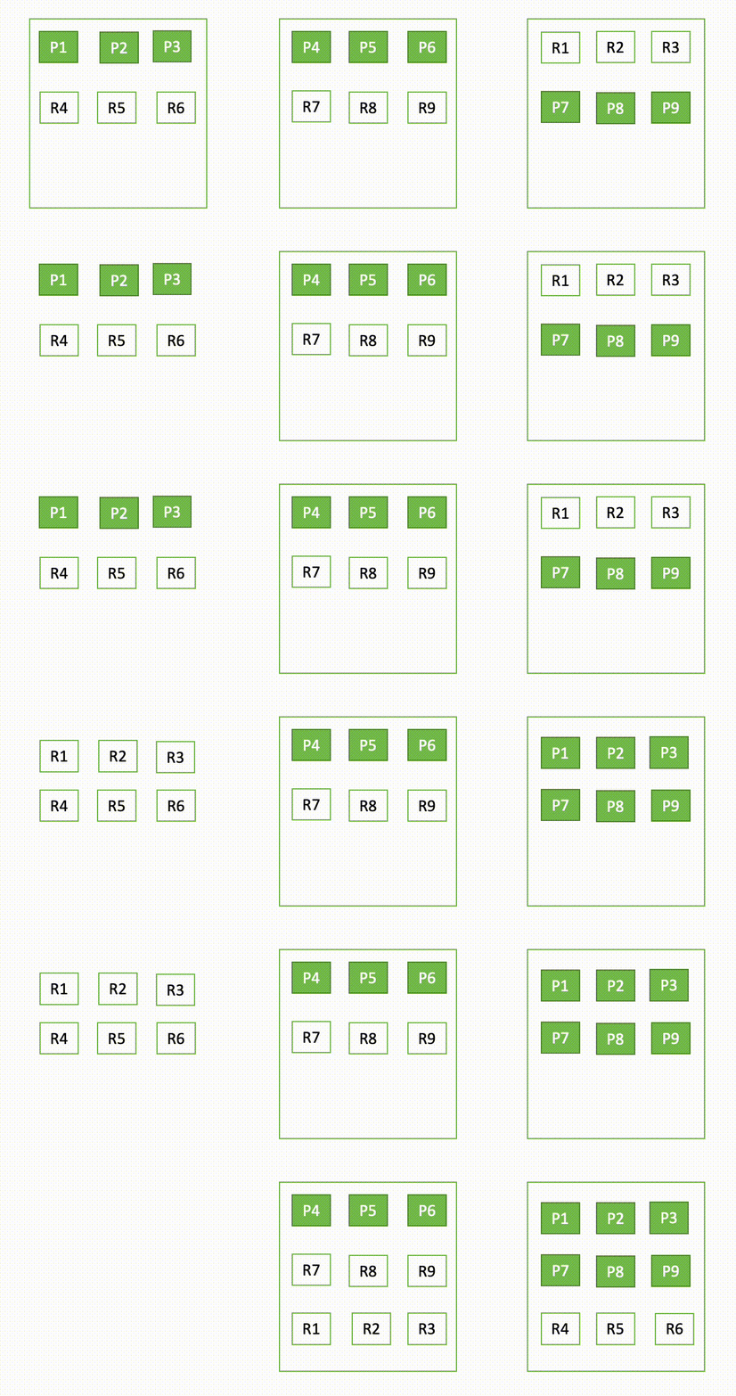
  2. Choose Roles.
  3. Choose the all_access role.OpenSearch Service All Access Role
  4. On the Mapped users tab, choose Manage mapping.OpenSearch Service Dashboard map role
  5. For Backend roles, enter the IAM role ARN created for the Firehose delivery stream.
  6. Choose Map.OpenSearch Service Dashboard Map role arn
  7. Now that mapping is complete, choose the menu icon, then choose Stack management.OpenSearch Service Dashboard Stack Management
  8. Choose Index Patterns, then choose Create index pattern.
  9. For Index pattern name, enter vpcflowlogs*.
  10. Choose Next step.OpenSearch Service Dashboard Create Index
  11. Navigate to the Discover menu option.You can see the VPC flow logs from your VPC in this dashboard. Now you can search and visualize the flow logs that are being streamed in near-real time to the OpenSearch Service domain.
    OpenSearch Service Dashboard Discover

Clean up

After you test out this solution, remember to delete all the resources you created to avoid incurring future charges:

  1. Delete your Amazon OpenSearch Service domain.
  2. Delete the VPC flow logs subscription.
  3. Delete the Firehose delivery stream.
  4. Delete the S3 bucket for the VPC flow logs backup and failed logs.
  5. If you created a new VPC and new resources in the VPC, delete the resources and VPC.

Conclusion

In this post, we walked through a solution of how integrate VPC flow logs with a Kinesis Data Firehose delivery stream and deliver it to an Amazon OpenSearch Service destination with no code and visualize it in OpenSearch Service Dashboards.

Try this new quick and hassle-free way of sending your VPC flow logs to an Amazon OpenSearch Service using Kinesis Data Firehose.


About the Author

Chaitanya Shah is a Sr. Technical Account Manager with AWS, based out of New York. He has over 22 years of experience working with enterprise customers. He loves to code and actively contributes to the AWS solutions labs to help customers solve complex problems. He provides guidance to AWS customers on best practices for their AWS Cloud migrations. He is also specialized in AWS data transfer and the data and analytics domain.

How to get best price performance from your Amazon Redshift Data Sharing deployment

Post Syndicated from BP Yau original https://aws.amazon.com/blogs/big-data/how-to-get-best-price-performance-from-your-amazon-redshift-data-sharing-deployment/

Amazon Redshift is a fast, scalable, secure, and fully-managed data warehouse that enables you to analyze all of your data using standard SQL easily and cost-effectively. Amazon Redshift Data Sharing allows customers to securely share live, transactionally consistent data in one Amazon Redshift cluster with another Amazon Redshift cluster across accounts and regions without needing to copy or move data from one cluster to another.

Amazon Redshift Data Sharing was initially launched in March 2021, and added support for cross-account data sharing was added in August 2021. The cross-region support became generally available in February 2022. This provides full flexibility and agility to share data across Redshift clusters in the same AWS account, different accounts, or different regions.

Amazon Redshift Data Sharing is used to fundamentally redefine Amazon Redshift deployment architectures into a hub-spoke, data mesh model to better meet performance SLAs, provide workload isolation, perform cross-group analytics, easily onboard new use cases, and most importantly do all of this without the complexity of data movement and data copies. Some of the most common questions asked during data sharing deployment are, “How big should my consumer clusters and producer clusters be?”, and “How do I get the best price performance for workload isolation?”. As workload characteristics like data size, ingestion rate, query pattern, and maintenance activities can impact data sharing performance, a continuous strategy to size both consumer and producer clusters to maximize the performance and minimize cost should be implemented. In this post, we provide a step-by-step approach to help you determine your producer and consumer clusters sizes for the best price performance based on your specific workload.

Generic consumer sizing guidance

The following steps show the generic strategy to size your producer and consumer clusters. You can use it as a starting point and modify accordingly to cater your specific use case scenario.

Size your producer cluster

You should always make sure that you properly size your producer cluster to get the performance that you need to meet your SLA. You can leverage the sizing calculator from the Amazon Redshift console to get a recommendation for the producer cluster based on the size of your data and query characteristic. Look for Help me choose on the console in AWS Regions that support RA3 node types to use this sizing calculator. Note that this is just an initial recommendation to get started, and you should test running your full workload on the initial size cluster and elastic resize the cluster up and down accordingly to get the best price performance.

Size and setup initial consumer cluster

You should always size your consumer cluster based on your compute needs. One way to get started is to follow the generic cluster sizing guide similar to the producer cluster above.

Setup Amazon Redshift data sharing

Setup data sharing from producer to consumer once you have both the producer and consumer cluster setup. Refer to this post for guidance on how to setup data sharing.

Test consumer only workload on initial consumer cluster

Test consumer only workload on the new initial consumer cluster. This can be done by pointing consumer applications, for example ETL tools, BI applications, and SQL clients, to the new consumer cluster and rerunning the workload to evaluate the performance against your requirements.

Test consumer only workload on different consumer cluster configurations

If the initial size consumer cluster meets or exceeds your workload performance requirements, then you can either continue to use this cluster configuration or you can test on smaller configurations to see if you can further reduce the cost and still get the performance that you need.

On the other hand, if the initial size consumer cluster fails to meet your workload performance requirements, then you can further test larger configurations to get the configuration that meets your SLA.

As a rule of thumb, size up the consumer cluster by 2x the initial cluster configuration incrementally until it meets your workload requirements.

Once you plan out what configuration you want to test, use elastic resize to resize the initial cluster to the target cluster configuration. After elastic resize is completed, perform the same workload test and evaluate the performance against your SLA. Select the configuration that meets your price performance target.

Test producer only workload on different producer cluster configurations

Once you move your consumer workload to the consumer cluster with the optimum price performance, there might be an opportunity to reduce the compute resource on the producer to save on costs.

To achieve this, you can rerun the producer only workload on 1/2x of the original producer size and evaluate the workload performance. Resizing the cluster up and down accordingly depends on the result, and then you select the minimum producer configuration that meets your workload performance requirements.

Re-evaluate after a full workload run over time

As Amazon Redshift continues evolving, and there are continuous performance and scalability improvement releases, data sharing performance will continue improving. Furthermore, numerous variables might impact the performance of data sharing queries. The following are just some examples:

  • Ingestion rate and amount of data change
  • Query pattern and characteristic
  • Workload changes
  • Concurrency
  • Maintenance activities, for example vacuum, analyze, and ATO

This is why you must re-evaluate the producer and consumer cluster sizing using the strategy above on occasion, especially after a full workload deployment, to gain the new best price performance from your cluster’s configuration.

Automated sizing solutions

If your environment involved more complex architecture, for example with multiple tools or applications (BI, ingestion or streaming, ETL, data science), then it might not feasible to use the manual method from the generic guidance above. Instead, you can leverage solutions in this section to automatically replay the workload from your production cluster on the test consumer and producer clusters to evaluate the performance.

Simple Replay utility will be leveraged as the automated solution to guide you through the process of getting the right producer and consumer clusters size for the best price performance.

Simple Replay is a tool for conducting a what-if analysis and evaluating how your workload performs in different scenarios. For example, you can use the tool to benchmark your actual workload on a new instance type like RA3, evaluate a new feature, or assess different cluster configurations. It also includes enhanced support for replaying data ingestion and export pipelines with COPY and UNLOAD statements. To get started and replay your workloads, download the tool from the Amazon Redshift GitHub repository.

Here we walk through the steps to extract your workload logs from the source production cluster and replay them in an isolated environment. This lets you perform a direct comparison between these Amazon Redshift clusters seamlessly and select the clusters configuration that best meet your price performance target.

The following diagram shows the solution architecture.

Architecutre for testing simple replay

Solution walkthrough

Follow these steps to go through the solution to size your consumer and producer clusters.

Size your production cluster

You should always make sure to properly size your existing production cluster to get the performance that you need to meet your workload requirements. You can leverage the sizing calculator from the Amazon Redshift console to get a recommendation on the production cluster based on the size of your data and query characteristic. Look for Help me choose on the console in AWS Regions that support RA3 node types to use this sizing calculator. Note that this is just an initial recommendation to get started. You should test running your full workload on the initial size cluster and elastic resize the cluster up and down accordingly to get the best price performance.

Identify the workload to be isolated

You might have different workloads running on your original cluster, but the first step is to identify the most critical workload to the business that we want to isolate. This is because we want to make sure that the new architecture can meet your workload requirements. This post is a good reference on a data sharing workload isolation use case that can help you decide which workload can be isolated.

Setup Simple Replay

Once you know your critical workload, you must enable audit logging in your production cluster where the critical workload identified above is running to capture query activities and store in Amazon Simple Storage Service (Amazon S3). Note that it may take up to three hours for the audit logs to be delivered to Amazon S3. Once the audit log is available, proceed to setup Simple Replay and then extract the critical workload from the audit log. Note that start_time and end_time could be used as parameters to filter out the critical workload if those workloads run in certain time periods, for example 9am to 11am. Otherwise it will extract all of the logged activities.

Baseline workload

Create a baseline cluster with the same configuration as the producer cluster by restoring from the production snapshot. The purpose of starting with the same configuration is to baseline the performance with an isolated environment.

Once the baseline cluster is available, replay the extracted workload in the baseline cluster. The output from this replay will be the baseline used to compare against subsequent replays on different consumer configurations.

Setup initial producer and consumer test clusters

Create a producer cluster with the same production cluster configuration by restoring from the production snapshot. Create a consumer cluster with the recommended initial consumer size from the previous guidance. Furthermore, setup data sharing between the producer and consumer.

Replay workload on initial producer and consumer

Replay the producer only workload on the initial size producer cluster. This can be achieved using the “Exclude” filter parameter to exclude consumer queries, for example the user that runs consumer queries.

Replay the consumer only workload on the initial size consumer cluster. This can be achieved using the “Include” filter parameter to exclude consumer queries, for example the user that runs consumer queries.

Evaluate the performance of these replays against the baseline and workload performance requirements.

Replay consumer workload on different configurations

If the initial size consumer cluster meets or exceeds your workload performance requirements, then you can either use this cluster configuration or you can follow these steps to test on smaller configurations to see if you can further reduce costs and still get the performance that you need.

Compare initial consumer performance results against your workload requirements:

  1. If the result exceeds your workload performance requirements, then you can reduce the size of the consumer cluster incrementally, starting with 1/2x, retry the replay and evaluate the performance, then resize up or down accordingly based on the result until it meets your workload requirements. The purpose is to get a sweet spot where you’re comfortable with the performance requirements and get the lowest price possible.
  2. If the result fails to meet your workload performance requirements, then you can increase the size of the cluster incrementally, starting with 2x the original size, retry the replay and evaluate the performance until it meets your workload performance requirements.

Replay producer workload on different configurations

Once you split your workloads out to consumer clusters, the load on the producer cluster should be reduced and you should evaluate your producer cluster’s workload performance to seek the opportunity to downsize to save on costs.

The steps are similar to consumer replay. Elastic resize the producer cluster incrementally starting with 1/2x the original size, replay the producer only workload and evaluate the performance, and then further resize up or down until it meets your workload performance requirements. The purpose is to get a sweet spot where you’re comfortable with the workload performance requirements and get the lowest price possible. Once you have the desired producer cluster configuration, retry replay consumer workloads on the consumer cluster to make sure that the performance wasn’t impacted by producer cluster configuration changes. Finally, you should replay both producer and consumer workloads concurrently to make sure that the performance is achieved in a full workload scenario.

Re-evaluate after a full workload run over time

Similar to the generic guidance, you should re-evaluate the producer and consumer clusters sizing using the previous strategy on occasion, especially after full workload deployment to gain the new best price performance from your cluster’s configuration.

Clean up

Running these sizing tests in your AWS account may have some cost implications because it provisions new Amazon Redshift clusters, which may be charged as on-demand instances if you don’t have Reserved Instances. When you complete your evaluations, we recommend deleting the Amazon Redshift clusters to save on costs. We also recommend pausing your clusters when they’re not in use.

Applying Amazon Redshift and data sharing best practices

Proper sizing of both your producer and consumer clusters will give you a good start to get the best price performance from your Amazon Redshift deployment. However, sizing isn’t the only factor that can maximize your performance. In this case, understanding and following best practices are equally important.

General Amazon Redshift performance tuning best practices are applicable to data sharing deployment. Make sure that your deployment follows these best practices.

There numerous data sharing specific best practices that you should follow to make sure that you maximize the performance. Refer to this post for more details.

Summary

There is no one-size-fits-all recommendation on producer and consumer cluster sizes. It varies by workloads and your performance SLA. The purpose of this post is to provide you with guidance for how you can evaluate your specific data sharing workload performance to determine both consumer and producer cluster sizes to get the best price performance. Consider testing your workloads on producer and consumer using simple replay before adopting it in production to get the best price performance.


About the Authors

BP Yau is a Sr Product Manager at AWS. He is passionate about helping customers architect big data solutions to process data at scale. Before AWS, he helped Amazon.com Supply Chain Optimization Technologies migrate its Oracle data warehouse to Amazon Redshift and build its next generation big data analytics platform using AWS technologies.

Sidhanth Muralidhar is a Principal Technical Account Manager at AWS. He works with large enterprise customers who run their workloads on AWS. He is passionate about working with customers and helping them architect workloads for costs, reliability, performance and operational excellence at scale in their cloud journey. He has a keen interest in Data Analytics as well.

Migrate Google BigQuery to Amazon Redshift using AWS Schema Conversion tool (SCT)

Post Syndicated from Jagadish Kumar original https://aws.amazon.com/blogs/big-data/migrate-google-bigquery-to-amazon-redshift-using-aws-schema-conversion-tool-sct/

Amazon Redshift is a fast, fully-managed, petabyte scale data warehouse that provides the flexibility to use provisioned or serverless compute for your analytical workloads. Using Amazon Redshift Serverless and Query Editor v2, you can load and query large datasets in just a few clicks and pay only for what you use. The decoupled compute and storage architecture of Amazon Redshift enables you to build highly scalable, resilient, and cost-effective workloads. Many customers migrate their data warehousing workloads to Amazon Redshift and benefit from the rich capabilities it offers. The following are just some of the notable capabilities:

  • Amazon Redshift seamlessly integrates with broader analytics services on AWS. This enables you to choose the right tool for the right job. Modern analytics is much wider than SQL-based data warehousing. Amazon Redshift lets you build lake house architectures and then perform any kind of analytics, such as interactive analytics, operational analytics, big data processing, visual data preparation, predictive analytics, machine learning (ML), and more.
  • You don’t need to worry about workloads, such as ETL, dashboards, ad-hoc queries, and so on, interfering with each other. You can isolate workloads using data sharing, while using the same underlying datasets.
  • When users run many queries at peak times, compute seamlessly scales within seconds to provide consistent performance at high concurrency. You get one hour of free concurrency scaling capacity for 24 hours of usage. This free credit meets the concurrency demand of 97% of the Amazon Redshift customer base.
  • Amazon Redshift is easy-to-use with self-tuning and self-optimizing capabilities. You can get faster insights without spending valuable time managing your data warehouse.
  • Fault Tolerance is inbuilt. All of the data written to Amazon Redshift is automatically and continuously replicated to Amazon Simple Storage Service (Amazon S3). Any hardware failures are automatically replaced.
  • Amazon Redshift is simple to interact with. You can access data with traditional, cloud-native, containerized, and serverless web services-based or event-driven applications and so on.
  • Redshift ML makes it easy for data scientists to create, train, and deploy ML models using familiar SQL. They can also run predictions using SQL.
  • Amazon Redshift provides comprehensive data security at no extra cost. You can set up end-to-end data encryption, configure firewall rules, define granular row and column level security controls on sensitive data, and so on.
  • Amazon Redshift integrates seamlessly with other AWS services and third-party tools. You can move, transform, load, and query large datasets quickly and reliably.

In this post, we provide a walkthrough for migrating a data warehouse from Google BigQuery to Amazon Redshift using AWS Schema Conversion Tool (AWS SCT) and AWS SCT data extraction agents. AWS SCT is a service that makes heterogeneous database migrations predictable by automatically converting the majority of the database code and storage objects to a format that is compatible with the target database. Any objects that can’t be automatically converted are clearly marked so that they can be manually converted to complete the migration. Furthermore, AWS SCT can scan your application code for embedded SQL statements and convert them.

Solution overview

AWS SCT uses a service account to connect to your BigQuery project. First, we create an Amazon Redshift database into which BigQuery data is migrated. Next, we create an S3 bucket. Then, we use AWS SCT to convert BigQuery schemas and apply them to Amazon Redshift. Finally, to migrate data, we use AWS SCT data extraction agents, which extract data from BigQuery, upload it into the S3 bucket, and then copy to Amazon Redshift.

Prerequisites

Before starting this walkthrough, you must have the following prerequisites:

  1. A workstation with AWS SCT, Amazon Corretto 11, and Amazon Redshift drivers.
    1. You can use an Amazon Elastic Compute Cloud (Amazon EC2) instance or your local desktop as a workstation. In this walkthrough, we’re using Amazon EC2 Windows instance. To create it, use this guide.
    2. To download and install AWS SCT on the EC2 instance that you previously created, use this guide.
    3. Download the Amazon Redshift JDBC driver from this location.
    4. Download and install Amazon Corretto 11.
  2. A GCP service account that AWS SCT can use to connect to your source BigQuery project.
    1. Grant BigQuery Admin and Storage Admin roles to the service account.
    2. Copy the Service account key file, which was created in the Google cloud management console, to the EC2 instance that has AWS SCT.
    3. Create a Cloud Storage bucket in GCP to store your source data during migration.

This walkthrough covers the following steps:

  • Create an Amazon Redshift Serverless Workgroup and Namespace
  • Create the AWS S3 Bucket and Folder
  • Convert and apply BigQuery Schema to Amazon Redshift using AWS SCT
    • Connecting to the Google BigQuery Source
    • Connect to the Amazon Redshift Target
    • Convert BigQuery schema to an Amazon Redshift
    • Analyze the assessment report and address the action items
    • Apply converted schema to target Amazon Redshift
  • Migrate data using AWS SCT data extraction agents
    • Generating Trust and Key Stores (Optional)
    • Install and start data extraction agent
    • Register data extraction agent
    • Add virtual partitions for large tables (Optional)
    • Create a local migration task
    • Start the Local Data Migration Task
  • View Data in Amazon Redshift

Create an Amazon Redshift Serverless Workgroup and Namespace

In this step, we create an Amazon Redshift Serverless workgroup and namespace. Workgroup is a collection of compute resources and namespace is a collection of database objects and users. To isolate workloads and manage different resources in Amazon Redshift Serverless, you can create namespaces and workgroups and manage storage and compute resources separately.

Follow these steps to create Amazon Redshift Serverless workgroup and namespace:

  • Navigate to the Amazon Redshift console.
  • In the upper right, choose the AWS Region that you want to use.
  • Expand the Amazon Redshift pane on the left and choose Redshift Serverless.
  • Choose Create Workgroup.
  • For Workgroup name, enter a name that describes the compute resources.
  • Verify that the VPC is the same as the VPC as the EC2 instance with AWS SCT.
  • Choose Next.

  • For Namespace name, enter a name that describes your dataset.
  • In Database name and password section, select the checkbox Customize admin user credentials.
    • For Admin user name, enter a username of your choice, for example awsuser.
    • For Admin user password: enter a password of your choice, for example MyRedShiftPW2022. 
  • Choose Next. Note that data in Amazon Redshift Serverless namespace is encrypted by default.
  • In the Review and Create page, choose Create.
  • Create an AWS Identity and Access Management (IAM) role and set it as the default on your namespace, as described in the following. Note that there can only be one default IAM role.
    • Navigate to the Amazon Redshift Serverless Dashboard.
    • Under Namespaces / Workgroups, choose the namespace that you just created.
    • Navigate toSecurity and encryption.
    • Under Permissions, choose Manage IAM roles.
    • Navigate to Manage IAM roles. Then, choose the Manage IAM roles drop-down and choose Create IAM role.
    • Under Specify an Amazon S3 bucket for the IAM role to access, choose one of the following methods:
      • Choose No additional Amazon S3 bucket to allow the created IAM role to access only the S3 buckets with a name starting with redshift.
      • Choose Any Amazon S3 bucket to allow the created IAM role to access all of the S3 buckets.
      • Choose Specific Amazon S3 buckets to specify one or more S3 buckets for the created IAM role to access. Then choose one or more S3 buckets from the table.
    • Choose Create IAM role as default. Amazon Redshift automatically creates and sets the IAM role as default.
  • Capture the Endpoint for the Amazon Redshift Serverless workgroup that you just created.

Create the S3 bucket and folder

During the data migration process, AWS SCT uses Amazon S3 as a staging area for the extracted data. Follow these steps to create the S3 bucket:

  • Navigate to the Amazon S3 console
  • Choose Create bucket. The Create bucket wizard opens.
  • For Bucket name, enter a unique DNS-compliant name for your bucket (e.g., uniquename-bq-rs). See rules for bucket naming when choosing a name.
  • For AWS Region, choose the region in which you created the Amazon Redshift Serverless workgroup.
  • Select Create Bucket.
  • In the Amazon S3 console, navigate to the S3 bucket that you just created (e.g., uniquename-bq-rs).
  • Choose “Create folder” to create a new folder.
  • For Folder name, enter incoming and choose Create Folder.

Convert and apply BigQuery Schema to Amazon Redshift using AWS SCT

To convert BigQuery schema to the Amazon Redshift format, we use AWS SCT. Start by logging in to the EC2 instance that we created previously, and then launch AWS SCT.

Follow these steps using AWS SCT:

Connect to the BigQuery Source

  • From the File Menu choose Create New Project.
  • Choose a location to store your project files and data.
  • Provide a meaningful but memorable name for your project, such as BigQuery to Amazon Redshift.
  • To connect to the BigQuery source data warehouse, choose Add source from the main menu.
  • Choose BigQuery and choose Next. The Add source dialog box appears.
  • For Connection name, enter a name to describe BigQuery connection. AWS SCT displays this name in the tree in the left panel.
  • For Key path, provide the path of the service account key file that was previously created in the Google cloud management console.
  • Choose Test Connection to verify that AWS SCT can connect to your source BigQuery project.
  • Once the connection is successfully validated, choose Connect.

Connect to the Amazon Redshift Target

Follow these steps to connect to Amazon Redshift:

  • In AWS SCT, choose Add Target from the main menu.
  • Choose Amazon Redshift, then choose Next. The Add Target dialog box appears.
  • For Connection name, enter a name to describe the Amazon Redshift connection. AWS SCT displays this name in the tree in the right panel.
  • For Server name, enter the Amazon Redshift Serverless workgroup endpoint captured previously.
  • For Server port, enter 5439.
  • For Database, enter dev.
  • For User name, enter the username chosen when creating the Amazon Redshift Serverless workgroup.
  • For Password, enter the password chosen when creating Amazon Redshift Serverless workgroup.
  • Uncheck the “Use AWS Glue” box.
  • Choose Test Connection to verify that AWS SCT can connect to your target Amazon Redshift workgroup.
  • Choose Connect to connect to the Amazon Redshift target.

Note that alternatively you can use connection values that are stored in AWS Secrets Manager. 

Convert BigQuery schema to an Amazon Redshift

After the source and target connections are successfully made, you see the source BigQuery object tree on the left pane and target Amazon Redshift object tree on the right pane.

Follow these steps to convert BigQuery schema to the Amazon Redshift format:

  • On the left pane, right-click on the schema that you want to convert.
  • Choose Convert Schema.
  • A dialog box appears with a question, The objects might already exist in the target database. Replace?. Choose Yes.

Once the conversion is complete, you see a new schema created on the Amazon Redshift pane (right pane) with the same name as your BigQuery schema.

The sample schema that we used has 16 tables, 3 views, and 3 procedures. You can see these objects in the Amazon Redshift format in the right pane. AWS SCT converts all of the BigQuery code and data objects to the Amazon Redshift format. Furthermore, you can use AWS SCT to convert external SQL scripts, application code, or additional files with embedded SQL.

Analyze the assessment report and address the action items

AWS SCT creates an assessment report to assess the migration complexity. AWS SCT can convert the majority of code and database objects. However, some of the objects may require manual conversion. AWS SCT highlights these objects in blue in the conversion statistics diagram and creates action items with a complexity attached to them.

To view the assessment report, switch from the Main view to the Assessment Report view as follows:

The Summary tab shows objects that were converted automatically, and objects that weren’t converted automatically. Green represents automatically converted or with simple action items. Blue represents medium and complex action items that require manual intervention.

The Action Items tab shows the recommended actions for each conversion issue. If you select an action item from the list, AWS SCT highlights the object to which the action item applies.

The report also contains recommendations for how to manually convert the schema item. For example, after the assessment runs, detailed reports for the database/schema show you the effort required to design and implement the recommendations for converting Action items. For more information about deciding how to handle manual conversions, see Handling manual conversions in AWS SCT. Amazon Redshift takes some actions automatically while converting the schema to Amazon Redshift. Objects with these actions are marked with a red warning sign.

You can evaluate and inspect the individual object DDL by selecting it from the right pane, and you can also edit it as needed. In the following example, AWS SCT modifies the RECORD and JSON datatype columns in BigQuery table ncaaf_referee_data to the SUPER datatype in Amazon Redshift. The partition key in the ncaaf_referee_data table is converted to the distribution key and sort key in Amazon Redshift.

Apply converted schema to target Amazon Redshift

To apply the converted schema to Amazon Redshift, select the converted schema in the right pane, right-click, and then choose Apply to database.

Migrate data from BigQuery to Amazon Redshift using AWS SCT data extraction agents

AWS SCT extraction agents extract data from your source database and migrate it to the AWS Cloud. In this walkthrough, we show how to configure AWS SCT extraction agents to extract data from BigQuery and migrate to Amazon Redshift.

First, install AWS SCT extraction agent on the same Windows instance that has AWS SCT installed. For better performance, we recommend that you use a separate Linux instance to install extraction agents if possible. For big datasets, you can use several data extraction agents to increase the data migration speed.

Generating trust and key stores (optional)

You can use Secure Socket Layer (SSL) encrypted communication with AWS SCT data extractors. When you use SSL, all of the data passed between the applications remains private and integral. To use SSL communication, you must generate trust and key stores using AWS SCT. You can skip this step if you don’t want to use SSL. We recommend using SSL for production workloads.

Follow these steps to generate trust and key stores:

  1. In AWS SCT, navigate to Settings → Global Settings → Security.
  2. Choose Generate trust and key store.
  3. Enter the name and password for trust and key stores and choose a location where you would like to store them.
  4. Choose Generate.

Install and configure Data Extraction Agent

In the installation package for AWS SCT, you find a sub-folder agent (\aws-schema-conversion-tool-1.0.latest.zip\agents). Locate and install the executable file with a name like aws-schema-conversion-tool-extractor-xxxxxxxx.msi.

In the installation process, follow these steps to configure AWS SCT Data Extractor:

  1. For Listening port, enter the port number on which the agent listens. It is 8192 by default.
  2. For Add a source vendor, enter no, as you don’t need drivers to connect to BigQuery.
  3. For Add the Amazon Redshift driver, enter YES.
  4. For Enter Redshift JDBC driver file or files, enter the location where you downloaded Amazon Redshift JDBC drivers.
  5. For Working folder, enter the path where the AWS SCT data extraction agent will store the extracted data. The working folder can be on a different computer from the agent, and a single working folder can be shared by multiple agents on different computers.
  6. For Enable SSL communication, enter yes. Choose No here if you don’t want to use SSL.
  7. For Key store, enter the storage location chosen when creating the trust and key store.
  8. For Key store password, enter the password for the key store.
  9. For Enable client SSL authentication, enter yes.
  10. For Trust store, enter the storage location chosen when creating the trust and key store.
  11. For Trust store password, enter the password for the trust store.
*************************************************
*                                               *
*     AWS SCT Data Extractor Configuration      *
*              Version 2.0.1.666                *
*                                               *
*************************************************
User name: Administrator
User home: C:\Windows\system32\config\systemprofile
*************************************************
Listening port [8192]: 8192
Add a source vendor [YES/no]: no
No one source data warehouse vendors configured. AWS SCT Data Extractor cannot process data extraction requests.
Add the Amazon Redshift driver [YES/no]: YES
Enter Redshift JDBC driver file or files: C:\Users\Administrator\Desktop\BQToRedshiftSCTProject\redshift-jdbc42-2.1.0.9.jar
Working folder [C:\Windows\system32\config\systemprofile]: C:\Users\Administrator\Desktop\BQToRedshiftSCTProject
Enable SSL communication [YES/no]: YES
Setting up a secure environment at "C:\Windows\system32\config\systemprofile". This process will take a few seconds...
Key store [ ]: C:\Users\Administrator\Desktop\BQToRedshiftSCTProject\TrustAndKeyStores\BQToRedshiftKeyStore
Key store password:
Re-enter the key store password:
Enable client SSL authentication [YES/no]: YES
Trust store [ ]: C:\Users\Administrator\Desktop\BQToRedshiftSCTProject\TrustAndKeyStores\BQToRedshiftTrustStore
Trust store password:
Re-enter the trust store password:

Starting Data Extraction Agent(s)

Use the following procedure to start extraction agents. Repeat this procedure on each computer that has an extraction agent installed.

Extraction agents act as listeners. When you start an agent with this procedure, the agent starts listening for instructions. You send the agents instructions to extract data from your data warehouse in a later section.

To start the extraction agent, navigate to the AWS SCT Data Extractor Agent directory. For example, in Microsoft Windows, double-click C:\Program Files\AWS SCT Data Extractor Agent\StartAgent.bat.

  • On the computer that has the extraction agent installed, from a command prompt or terminal window, run the command listed following your operating system.
  • To check the status of the agent, run the same command but replace start with status.
  • To stop an agent, run the same command but replace start with stop.
  • To restart an agent, run the same RestartAgent.bat file.

Register the Data Extraction Agent

Follow these steps to register the Data Extraction Agent:

  1. In AWS SCT, change the view to Data Migration view (other) and choose + Register.
  2. In the connection tab:
    1. For Description, enter a name to identify the Data Extraction Agent.
    2. For Host name, if you installed the Data Extraction Agent on the same workstation as AWS SCT, enter 0.0.0.0 to indicate local host. Otherwise, enter the host name of the machine on which the AWS SCT Data Extraction Agent is installed. It’s recommended to install the Data Extraction Agents on Linux for better performance.
    3. For Port, enter the number entered for the Listening Port when installing the AWS SCT Data Extraction Agent.
    4. Select the checkbox to use SSL (if using SSL) to encrypt the AWS SCT connection to the Data Extraction Agent.
  3. If you’re using SSL, then in the SSL Tab:
    1. For Trust store, choose the trust store name created when generating Trust and Key Stores (optionally, you can skip this if SSL connectivity isn’t needed).
    2. For Key Store, choose the key store name created when generating Trust and Key Stores (optionally, you can skip this if SSL connectivity isn’t needed).
  4. Choose Test Connection.
  5. Once the connection is validated successfully, choose Register.

Add virtual partitions for large tables (optional)

You can use AWS SCT to create virtual partitions to optimize migration performance. When virtual partitions are created, AWS SCT extracts the data in parallel for partitions. We recommend creating virtual partitions for large tables.

Follow these steps to create virtual partitions:

  1. Deselect all objects on the source database view in AWS SCT.
  2. Choose the table for which you would like to add virtual partitioning.
  3. Right-click on the table, and choose Add Virtual Partitioning.
  4. You can use List, Range, or Auto Split partitions. To learn more about virtual partitioning, refer to Use virtual partitioning in AWS SCT. In this example, we use Auto split partitioning, which generates range partitions automatically. You would specify the start value, end value, and how big the partition should be. AWS SCT determines the partitions automatically. For a demonstration, on the Lineorder table:
    1. For Start Value, enter 1000000.
    2. For End Value, enter 3000000.
    3. For Interval, enter 1000000 to indicate partition size.
    4. Choose Ok.

You can see the partitions automatically generated under the Virtual Partitions tab. In this example, AWS SCT automatically created the following five partitions for the field:

    1. <1000000
    2. >=1000000 and <=2000000
    3. >2000000 and <=3000000
    4. >3000000
    5. IS NULL

Create a local migration task

To migrate data from BigQuery to Amazon Redshift, create, run, and monitor the local migration task from AWS SCT. This step uses the data extraction agent to migrate data by creating a task.

Follow these steps to create a local migration task:

  1. In AWS SCT, under the schema name in the left pane, right-click on Standard tables.
  2. Choose Create Local task.
  3. There are three migration modes from which you can choose:
    1. Extract source data and store it on a local pc/virtual machine (VM) where the agent runs.
    2. Extract data and upload it on an S3 bucket.
    3. Choose Extract upload and copy, which extracts data to an S3 bucket and then copies to Amazon Redshift.
  4. In the Advanced tab, for Google CS bucket folder enter the Google Cloud Storage bucket/folder that you created earlier in the GCP Management Console. AWS SCT stores the extracted data in this location.
  5. In the Amazon S3 Settings tab, for Amazon S3 bucket folder, provide the bucket and folder names of the S3 bucket that you created earlier. The AWS SCT data extraction agent uploads the data into the S3 bucket/folder before copying to Amazon Redshift.
  6. Choose Test Task.
  7. Once the task is successfully validated, choose Create.

Start the Local Data Migration Task

To start the task, choose the Start button in the Tasks tab.

  • First, the Data Extraction Agent extracts data from BigQuery into the GCP storage bucket.
  • Then, the agent uploads data to Amazon S3 and launches a copy command to move the data to Amazon Redshift.
  • At this point, AWS SCT has successfully migrated data from the source BigQuery table to the Amazon Redshift table.

View data in Amazon Redshift

After the data migration task executes successfully, you can connect to Amazon Redshift and validate the data.

Follow these steps to validate the data in Amazon Redshift:

  1. Navigate to the Amazon Redshift QueryEditor V2.
  2. Double-click on the Amazon Redshift Serverless workgroup name that you created.
  3. Choose the Federated User option under Authentication.
  4. Choose Create Connection.
  5. Create a new editor by choosing the + icon.
  6. In the editor, write a query to select from the schema name and table name/view name you would like to verify. Explore the data, run ad-hoc queries, and make visualizations and charts and views.

The following is a side-by-side comparison between source BigQuery and target Amazon Redshift for the sports data-set that we used in this walkthrough.

Clean up up any AWS resources that you created for this exercise

Follow these steps to terminate the EC2 instance:

  1. Navigate to the Amazon EC2 console.
  2. In the navigation pane, choose Instances.
  3. Select the check-box for the EC2 instance that you created.
  4. Choose Instance state, and then Terminate instance.
  5. Choose Terminate when prompted for confirmation.

Follow these steps to delete Amazon Redshift Serverless workgroup and namespace

  1. Navigate to Amazon Redshift Serverless Dashboard.
  2. Under Namespaces / Workgroups, choose the workspace that you created.
  3. Under Actions, choose Delete workgroup.
  4. Select the checkbox Delete the associated namespace.
  5. Uncheck Create final snapshot.
  6. Enter delete in the delete confirmation text box and choose Delete.

Follow these steps to delete the S3 bucket

  1. Navigate to Amazon S3 console.
  2. Choose the bucket that you created.
  3. Choose Delete.
  4. To confirm deletion, enter the name of the bucket in the text input field.
  5. Choose Delete bucket.

Conclusion

Migrating a data warehouse can be a challenging, complex, and yet rewarding project. AWS SCT reduces the complexity of data warehouse migrations. Following this walkthrough, you can understand how a data migration task extracts, downloads, and then migrates data from BigQuery to Amazon Redshift. The solution that we presented in this post performs a one-time migration of database objects and data. Data changes made in BigQuery when the migration is in progress won’t be reflected in Amazon Redshift. When data migration is in progress, put your ETL jobs to BigQuery on hold or replay the ETLs by pointing to Amazon Redshift after the migration. Consider using the best practices for AWS SCT.

AWS SCT has some limitations when using BigQuery as a source. For example, AWS SCT can’t convert sub queries in analytic functions, geography functions, statistical aggregate functions, and so on. Find the full list of limitations in the AWS SCT user guide. We plan to address these limitations in future releases. Despite these limitations, you can use AWS SCT to automatically convert most of your BigQuery code and storage objects.

Download and install AWS SCT, sign in to the AWS Console, checkout Amazon Redshift Serverless, and start migrating!


About the authors

Cedrick Hoodye is a Solutions Architect with a focus on database migrations using the AWS Database Migration Service (DMS) and the AWS Schema Conversion Tool (SCT) at AWS. He works on DB migrations related challenges. He works closely with EdTech, Energy, and ISV business sector customers to help them realize the true potential of DMS service. He has helped migrate 100s of databases into the AWS cloud using DMS and SCT.

Amit Arora is a Solutions Architect with a focus on Database and Analytics at AWS. He works with our Financial Technology and Global Energy customers and AWS certified partners to provide technical assistance and design customer solutions on cloud migration projects, helping customers migrate and modernize their existing databases to the AWS Cloud.

Jagadish Kumar is an Analytics Specialist Solution Architect at AWS focused on Amazon Redshift. He is deeply passionate about Data Architecture and helps customers build analytics solutions at scale on AWS.

Anusha Challa is a Senior Analytics Specialist Solution Architect at AWS focused on Amazon Redshift. She has helped many customers build large-scale data warehouse solutions in the cloud and on premises. Anusha is passionate about data analytics and data science and enabling customers achieve success with their large-scale data projects.

Using Workflows to Build, Test, and Deploy with Amazon CodeCatalyst

Post Syndicated from Kumar Karra original https://aws.amazon.com/blogs/devops/using-workflows-to-build-test-and-deploy-with-amazon-codecatalyst/

Amazon CodeCatalyst workflows are continuous integration and continuous delivery (CI/CD) pipelines that enable you to easily build, test and deploy applications. CodeCatalyst was announced at re:Invent 2022 and is currently in preview.

Introduction:

I recently read The Unicorn Project, the follow-up to the bestselling title The Phoenix Project from Gene Kim. After a few years at Amazon, I had forgotten how some companies write software, but it all came back to me as I read. In the book, the main character, Maxine, struggles with a complicated software development lifecycle (SLDC) after joining a new team. Some of the challenges she encounters include:

  • Continually delivering high-quality updates is complicated and slow
  • Collaborating efficiently with others is challenging
  • Managing application environments is increasingly complex
  • Setting up a new project is a time consuming chore

Amazon CodeCatalyst can help address all of these issues. CodeCatalyst is an integrated DevOps service that makes it easy for development teams to quickly build and deliver applications on AWS. Over the next few weeks, my colleagues and I will release a series of blog posts describing the individual features of CodeCatalyst and how they will help you overcome the challenges that Maxine encountered in The Unicorn Project. In this first post, I focus on Workflows and address the first bullet above, “continually delivering high-quality updates is complicated and slow”.

CodeCatalyst Workflows help you reliably deliver high-quality application updates frequently, quickly and securely. CodeCatalyst uses a visual editor — or if you prefer YAML — to quickly assemble and configure actions to compose workflows that automate your CI/CD pipeline, test reporting and other manual processes. Workflows use provisioned compute, lambda compute, custom container images and a managed build infrastructure to scale execution easily without sacrificing flexibility

Prerequisites

If you would like to follow along with this walkthrough, you will need to:

Walkthrough

For this walkthrough, I am going use the Modern Three-tier Web Application blueprint. A CodeCatalyst blueprint provides a template for a new project. If you would like to follow along, you can launch the blueprint as described in Creating a project in Amazon CodeCatalyst.  This will deploy the architecture shown below.

Modern Three-tier Web Application architecture including a presentation, application and data layer

Figure 1. Modern Three-tier Web Application architecture including a presentation, application and data layer

Once the new project is launched, navigate to CI/CD > Workflows. You will see two workflows listed. Click on  ApplicationDeploymentPipeline and you will be presented with the workflow pictured below. The workflow consists of six actions: 1) ensures that CDK is configured in the account; 2) builds the backend, written in Python, including unit tests; 3) deploys the backend to either AWS Lambda or AWS Fargate depending on which you selected when you launched the project; 4) runs a series of integration tests on the deployed backend; 5) builds the frontend, written with Vue, including unit tests; and finally, 6) deploys the frontend to Amazon Simple Storage Service (Amazon S3) and Amazon CloudFront.

Six step Workflow described in the prior paragraph

Figure 2. Six step Workflow described in the prior paragraph

Let’s look at a few of these actions. If you click on each action you will see details about the workflow execution. For example, I clicked on build_backend. On the logs tab, I can see the build action executes a series of steps. In this example,  pip installs requirements and then pytest and coverage run a series of unit test. If this had been a compiled language — like Java or .NET — there would have been a build step as well.

Logs from the build action including pip, pytest, and coverage

Figure 3. Logs from the build action including pip, pytest, and coverage

If I switch to the Reports tab, I see the result of the unit tests as well as code and branch coverage. In each case the test has exceeded the pass rate, indicated by the black bar on the graph. If they had not, the build would have failed.

Results of the unit tests including code and branch coverage

Figure 4. Results of the unit tests including code and branch coverage

Next, let’s examine how the workflow is defined by clicking on the Edit button in the top right corner of the screen. If the editor opens in YAML mode, switch to Visual mode using the toggle above the code. If I click on WorkflowSource, I see that the Workflow is triggered by a push to the main branch. I could add additional triggers. CodeCatalyst supports triggering on Push or Pull Request. In addition, I can trigger off multiple branches, including wildcards (e.g. “release-.*”).  Finally, I can trigger branches when only some files in a repository change (e.g. "src/.*")

Trigger configuration showing various options

Figure 5. Trigger configuration showing various options

Now, let’s look at the build_frontend action. This is a build action, similar to the build_backend action you looked at earlier. On the Configure tab I can see the Shell commands that will be executed during the build. Remember that the frontend is written using Vue. Here I can see  npm install used to install dependencies, npm run test:unit used to run tests, and finally npm run build-only to build the Single Page App (SPA). The resulting artifacts are passed to subsequent actions in the Workflow.

Shell commands run in the build action

Figure 6. Shell commands run in the build action

Next, let’s look at the integration_test action. A managed test action is very similar to a build action, defining a series of commands to execute. On the configuration tab (not shown), I can see that this action is again running pytest. Switching to the Outputs tab, I see that CodeCatalyst is configured to automatically discover the test reports generated by pytest and other test frameworks. In addition, I have defined a minimum pass rate of 100%. This means that the workflow should fail if any of the integration tests fail.

Test report configuration dialog including success criteria

Figure 7. Test report configuration dialog including success criteria

Finally, let’s examine the deploy_frontend action. Note that all of the actions you have looked at so far include a series of commands to run in their configuration. While these actions are highly flexible, CodeCatalyst also supports purpose built actions. The cdk-deploy action is an example of this. As the name implies, this action deploys AWS Cloud Development Kit (CDK) resources. I could have called cdk deploy from the shell commands in a build action. However, using the purpose built action is easier. CodeCatalyst supports many purpose build actions developed by AWS as well as third parties. Click on the + sign in the top left corner of the screen to see a few examples.  In addition, CodeCatalyst supports GitHub actions, but that is a topic for another post.

Cleanup

If you have been following along with this workflow, you should delete the resources you deployed so you do not continue to incur charges (See pricing page for more details). First, delete the two stacks that CDK deployed using the AWS CloudFormation console in the AWS account you associated when you launched the blueprint. These stacks will have names like mysfitsXXXXXWebStack and mysfitsXXXXXAppStack. Second, delete the project from CodeCatalyst by navigating to Project settings and clicking the Delete project button.

Conclusion

In this post, you learned how CodeCatalyst can help you rapidly assemble automation workflows by configuring composable, pre-built actions into CI/CD pipelines. I examined actions to build, test and deploy both frontend and backend applications. In future posts, I will discuss how CodeCatalyst can address the rest of the challenges Maxine encountered in The Unicorn Project.

About the authors:

Kumar Karra

Kumar Karra is a Field Solutions Architect for AWS Small and Medium Business Customers. He has a strong background in designing and developing applications for small consumer facing customers to large mission critical applications for enterprises. He specialized in Builder’s Experience tools and enjoys helping customer shorten their time to value by guiding them on strategies to implement fast, repeatable, testable, and scalable tools and architectures.

Kawshik Sarkar

Kawshik Sarkar is a Field Solutions Architect for AWS Small Medium Business customers . He helps customers by designing solutions using AWS cloud services , to enhance their user experience ,maximize outcomes and improve business agility . He enjoys music , podcasts ,tennis  and being outdoors

Divya Konaka Satyapal

Divya Konaka Satyapal is a Sr.Technical Account Manager for WWPS Edtech/EDU customers. Her expertise lies in DevOps and Serverless architectures. She works with customers heavily on cost optimization and overall operational excellence to accelerate their cloud journey. Outside of work, she enjoys traveling and playing tennis.

Simplify private network access for solutions using Amazon OpenSearch Service managed VPC endpoints

Post Syndicated from Aish Gunasekar original https://aws.amazon.com/blogs/big-data/simplify-private-network-access-for-solutions-using-amazon-opensearch-service-managed-vpc-endpoints/

Amazon OpenSearch Service makes it easy for you to perform interactive log analytics, real-time application monitoring, website search, and more. Amazon OpenSearch is an open source, distributed search and analytics suite. Amazon OpenSearch Service offers the latest versions of OpenSearch, support for 19 versions of Elasticsearch (1.5 to 7.10 versions), as well as visualization capabilities powered by OpenSearch Dashboards and Kibana (1.5 to 7.10 versions). Amazon OpenSearch Service currently has tens of thousands of active customers with hundreds of thousands of clusters under management processing trillions of requests per month.

To meet the needs of customers who want simplicity in their network setup with the Amazon OpenSearch Service, you can now use Amazon OpenSearch Service-managed virtual private cloud (VPC) endpoints (powered by AWS PrivateLink) to connect to your applications using Amazon OpenSearch Service domains launched in Amazon Virtual Private Cloud (VPC). With Amazon OpenSearch Service-managed VPC endpoints, you can privately access your Amazon OpenSearch Service domain from multiple VPCs in your account or other AWS accounts based on your application needs without configuring other services features such as VPC peering, AWS Transit Gateway (TGW), or other more complex network routing strategies that place operational burden on your support and engineering teams.

The feature is built using AWS PrivateLink. AWS PrivateLink provides private connectivity between VPCs, supported AWS services, and your on-premises networks without exposing your traffic to the public internet. It provides you with the means to connect multiple application deployments effortlessly to your Amazon OpenSearch Service domains.

This post introduces Amazon OpenSearch Service-managed VPC endpoints that build on top of AWS PrivateLink and shows how you can access a private Amazon OpenSearch Service from one or more VPCs hosted in the same account, or even VPCs hosted in other AWS accounts using AWS PrivateLink managed by Amazon OpenSearch Service.

­­­­Amazon OpenSearch Service managed VPC endpoints

Before the launch of Amazon OpenSearch Service managed VPC endpoints, if you needed to gain access to your domain outside of your VPC, you had three options:

  • Use VPC peering to connect your VPC with other VPCs
  • Use AWS Transit Gateway to connect your VPC with other VPCs
  • Create your own implementation of an AWS PrivateLink setup

The first two options require you to setup your VPCs so that the Classless Inter-Domain Routing (CIDR) block ranges don’t overlap. If they did, then your options are more complicated. The third option, create your own implementation of AWS PrivateLink, involve configuring a network load balancer (NLB) and associating a target group with the NLB as one of the steps in the setup. The architecture discussed in this post, demonstrates these additional layers of complexity.

With Amazon OpenSearch Service managed VPC endpoints (i.e., powered by AWS PrivateLink), these complex setups and processes are no longer needed!

You can access your Amazon OpenSearch Service private domain as if it were deployed in all the VPCs that you want to connect to your domain. If you need private connectivity from your on-premises hybrid deployments, then AWS PrivateLink helps you bring access from your Amazon OpenSearch Service domain to your data centers with minimal effort.

By using AWS PrivateLink with Amazon OpenSearch Service, you can realize the following benefits:

  • You simplify your network architecture between hybrid, multi-VPC, and multi account solutions
  • You address a multitude of compliance concerns by better controlling the traffic that moves between your solutions and Amazon OpenSearch Service domains

Shared search cluster for multiple development teams

Imagine that your company hosts a service as a software (SaaS) application that provides a search application programming interface (API) for the healthcare industry. Each team works on a different function of the API. The development teams API team 1 and API team 2 are in two different AWS accounts and each has their own VPCs within these accounts. Another team (data refinement team) works on the ingestion and data refinement to populate the Amazon OpenSearch Service domain hosted in the same account as API team 2 but in different VPC. Each team shares the domain during the development cycles to save costs and foster collaboration on the data modeling.

Solution overview

Self-managed AWS PrivateLink architecture to connect different VPCs

In this scenario prior to Amazon OpenSearch Service manage VPC endpoints (i.e., powered by AWS PrivateLink), you would have to create the following items:

  1. Deploy an NLB in your VPC
  2. Create a target group that points to the IP addresses of the Elastic Network Interfaces (ENIs), which the Amazon OpenSearch Service creates in your VPC and is used to launch the Amazon OpenSearch Service
  3. Create an AWS PrivateLink deployment and reference your newly created NLB

When you implement the NLB, a target group can only reference IP addresses, an Amazon EC2 instance, or an Application Load Balancer (ALB). If you referenced the IP addresses as targets, then you had to build a process that detected the changes in the IP address if the domain changed due to service initiated or self-initiated blue/green deployments. You must maintain yet another complex process to ensure that you always have active ENIs with which to point your target groups or you lose connectivity.

Typically, customers use an AWS Lambda with scheduled events in Amazon CloudWatch. This means that you use the AWS Lambda to detect the current state where the ENIs that provided the IP addresses were marked as active for the description that matched the ENIs your domain creates. You schedule AWS Lambda to wake up within the time to live (TTL) of the Domain Name Service (DNS) settings (typically 60 seconds) and compare the existing IP addresses in the target group with any new ones found when you query all ENIs with a description referencing your domain in the VPC. You then build a new target group with the deltas and you swap the target groups and drop the old one. It’s tricky, it’s complex, and you have to maintain the solution!

With the new simplified networking architecture, your teams go through the following steps.

OpenSearch Service managed VPC endpoints architecture (powered by AWS PrivateLink)

Since the Amazon OpenSearch Service takes care of the infrastructure described previously — but not necessarily on the same implementation — all you really need to concern yourself with is creating the connections using the instructions in our service documentation.

Once you complete the steps in the instructions and remove your own implementation, your architecture is then simplified as seen in the following diagram.

Once you complete the steps in the instructions and remove your own implementation, your architecture is then simplified.

At this point, the development teams (API team 1 and API team 2) can access the Amazon OpenSearch cluster via Amazon OpenSearch Service Managed VPC Endpoint. This option is highly scalable with a simplified network architecture in which you don’t have to worry about managing a NLB, or setting up target groups and the additional resources. If the number of development teams and VPCs grow in the future, you associate the domain with the associated interface VPC endpoint. You can access services in VPCs in same or different accounts, even if there are overlapping CIDR Block IP ranges.

Conclusion

In this post, we walked through the architectural design of accessing Amazon OpenSearch cluster from different VPCs across different accounts using OpenSearch Service-managed VPC endpoint (AWS PrivateLink). Using Transit Gateway, self-managed AWS PrivateLink or VPC peering required complex networking strategies that increased operation burden. With the introduction of VPC endpoints for Amazon OpenSearch Service, the complexity of your solutions is greatly simplified and what’s even better, it’s managed for you!


About the authors

Aish Gunasekar is a Specialist Solutions architect with a focus on Amazon OpenSearch Service. Her passion at AWS is to help customers design highly scalable architectures and help them in their cloud adoption journey. Outside of work, she enjoys hiking and baking.


Kevin Fallis (@AWSCodeWarrior) is an AWS specialist search solutions architect.  His passion at AWS is to help customers leverage the correct mix of AWS services to achieve success for their business goals. His after-work activities include family, DIY projects, carpentry, playing drums, and all things music.

Scale read and write workloads with Amazon Redshift

Post Syndicated from Harsha Tadiparthi original https://aws.amazon.com/blogs/big-data/scale-read-and-write-workloads-with-amazon-redshift/

Amazon Redshift is a fast, fully managed, petabyte-scale cloud data warehouse that enables you to analyze large datasets using standard SQL. The concurrency scaling feature in Amazon Redshift automatically adds and removes capacity by adding concurrency scaling to handle demands from thousands of concurrent users, thereby providing consistent SLAs for unpredictable and spiky workloads such as BI reports, dashboards, and other analytics workloads.

Until now, concurrency scaling only supported auto scaling for read queries; write queries had to run on the main cluster. Now, we are extending concurrency scaling to support auto scaling for common write queries including COPY, INSERT, UPDATE, and DELETE. This is available on Amazon Redshift RA3 provisioned instance types in the Regions where concurrency scaling is available. Amazon Redshift serverless comes with built in dynamic auto scaling capability for read workload scaling.

In this post, we discuss how to enable concurrency scaling to offer consistent SLAs for concurrent workloads such as data loads, ETL (extract, transform, and load), and data processing with reduced queue times.

Concurrency scaling overview

With concurrency scaling, Amazon Redshift automatically and elastically scales query processing power to provide consistently fast performance for hundreds of concurrent queries. Concurrency scaling resources are added to your Amazon Redshift cluster transparently in seconds, as concurrency increases, to serve sudden spikes in concurrent requests with fast performance without wait time. When the workload demand subsides, Amazon Redshift automatically shuts down concurrency scaling resources to save you cost.

The following diagram shows how concurrency scaling works at a high level.

The workflow contains the following steps:

  1. All queries go to the main cluster.
  2. When queries in the designated workload management (WLM) queue begin queuing, Amazon Redshift automatically routes eligible queries to the new clusters, enabling concurrency scaling.
  3. Amazon Redshift automatically spins up a new cluster, processes waiting queries, and shuts down the concurrency scaling cluster when no longer needed.

Enable Amazon Redshift concurrency scaling

You can manage concurrency scaling at the WLM queue level, where you set concurrency scaling policies for specific queues. When concurrency scaling is enabled for a queue, eligible write and read queries are sent to concurrency scaling clusters without having to wait for resources to free up on the main Amazon Redshift cluster. Amazon Redshift handles spinning up concurrency scaling clusters, routing of the queries to the transient clusters, and relinquishing the concurrency clusters.

You can enable concurrency scaling on both automatic and manual WLM.

You first need to determine which parameter group your cluster is. To do so, complete the following steps:

  1. On the Amazon Redshift console, choose Clusters in the navigation pane.
  2. Choose your cluster.
  3. On the Properties tab, note the parameter group associated to the cluster.
    Now you can configure your WLM parameters.
  4. Under Configurations in the navigation pane, choose Workload management.
  5. Choose the parameter group associated to the cluster.If you’re using the default parameter group default.redshift-1.0, you need to create a custom parameter group and assign that to the cluster. The default parameter group has preset values for each of its parameters, and it can’t be modified.
  6. On the Parameters tab, you can choose between 1–10 max_concurrency_scaling_clusters.This is the max number of concurrent Amazon Redshift clusters you can have running at the same time. Ten is the soft limit; this limit can be increased by submitting a service limit increase request with a support case.
  7. On the Workload management tab, choose auto mode for the concurrency scaling cluster.

Example use cases

In this section, we use three use cases to help you understand how concurrency scaling for read and write heavy workloads can seamlessly scale to improve workload performance SLAs.

We used a 3 TB Cloud DW benchmark dataset. The test included a total of 103 concurrent queries, with each run using a separate database connection. The 103 queries constituted 60 queries from the 99 TPC-DS queries and 43 write queries, with a mix of copy, insert, update and delete statements. We used RA3.4xlarge 5 compute nodes.

The following scenarios showcase how concurrency scaling for reads and writes can seamlessly auto scale and positively impact a heavy concurrent mixed workload:

  • All queries triggered concurrently with concurrency scaling turned off
  • All queries triggered concurrently with concurrency scaling cluster limit set to 5 clusters
  • All queries triggered concurrently with concurrency scaling cluster limit set to 10 clusters

Scenario 1: All queries triggered concurrently with concurrency scaling turned off

In this benchmark test, all queries completed in 299 minutes. The following are the test details.

The Amazon Redshift query optimizer turned the 103 queries into 257 sub-queries for better performance in this run. Amazon Redshift continuous to learn from operational statistics to optimize your workload.

The following screenshot shows how Amazon Redshift auto WLM mode chose to run 16 queries concurrently while queuing the rest. Because concurrency scaling is turned off, no additional clusters are spun up and the queries continue to wait for running queries to complete before they can be processed. Notice the number of queries queued stayed at a higher number for a long period of time and eventually lowered as only a few queries could concurrently run.

No additional concurrent clusters spun up during the window of the workload, as seen in the following screenshot, requiring the primary cluster to process all the queries.

Scenario 2: All queries triggered concurrently with concurrency scaling cluster max limit set to 5 clusters

In this test, all queries completed in 49 minutes.

The following screenshot depicts significant queuing. Within seconds, five additional Amazon Redshift clusters are spun up into ready state, allowing 53 queries to run simultaneously. This number can change in your cluster based on the query types. Notice the number of queries queued starts lowering as more queries are completed using the five additional clusters.

Over time, the concurrency scaling clusters start to wind down progressively to 0 as the queries no longer waited.

Scenario 3: All queries triggered concurrently with concurrency scaling cluster limit set to 10 clusters

In this test, all queries completed in 28 minutes.

The following screenshot depicts significant queuing. Within seconds, 10 additional Amazon Redshift clusters are spun up into ready state, allowing multiple queries to run simultaneously. This number can change in your cluster based on the query types. Notice the number of queries queued starts lowering as more queries are completed using the five additional clusters.

Over time, the concurrency scaling clusters start to wind down progressively to 0 as the queries no longer waited.

Test results review

The following table summarizes our test results.

. Test Scenario 1 Test Scenario 2 Test Scenario 3
Total Workload Completion Time 299 Minutes 49 Minutes 28 Minutes

The test results reveal how concurrency scaling for a mixed workload of reads and writes lowered the total workload completion time from 299 minutes to 28 minutes, which is more than 10 times an improvement in SLAs while being cost effective by only paying for the additional clusters when scaling is necessary.

Monitor concurrency scaling

One method to monitor concurrency scaling is via system views. To monitor which queries benefitted from concurrency scaling, you can use concurrency_scaling_status from stl_query. Concurrency scaling of 1 indicates that the query ran on a concurrency scaling cluster. To monitor concurrency scaling usage, you can use the SVCS_CONCURRENCY_SCALING_USAGE system view.

The Amazon CloudWatch metrics ConcurrencyScalingActiveClusters and ConcurrencyScalingSeconds enable you to set up monitoring of concurrency scaling usage. For more information, refer to Monitoring Amazon Redshift using CloudWatch metrics.

Configure usage limit

With every 24 hours used of the main Amazon Redshift cluster, you accrue 1 hour of concurrency scaling credit. This free credit can be used by both read and write queries. For any usage that exceeds the accrued free usage credits, you’re billed on a per-second basis based on the on-demand rate of your Amazon Redshift cluster. You can apply cost controls for concurrency scaling at the cluster level. You can choose to create multiple queues for ETL, Dashboard, and adhoc workload. With this you can choose to turn on concurrency scaling for selective queues.

As shown in the following screenshot, you can choose a time period (daily, weekly, or monthly) and specify the desired usage limit. You can then choose an action option (Alert, Log to system table, or Disable feature). For more details on how to set cost controls for concurrency scaling, refer to Manage and control your cost with Amazon Redshift Concurrency Scaling and Spectrum.

Summary

In this post, we showed how you can enable concurrency scaling to help you meet the SLAs for both read and write workloads by seamlessly scaling out to the maximum number of clusters you configured, thereby increasing your cluster throughput while controlling your costs. Concurrency scaling with read and write capability can enable you to handle a number of scenarios, such as sudden increases in the volume of data in your data pipeline, backfill operations, ad hoc reporting, and month end processing. It’s now time to put this learning into action and begin optimizing your Redshift cluster(s) for both read and write throughput!


About the Authors

Harsha Tadiparthi is a specialist Principal Solutions Architect, Analytics at AWS. He enjoys solving complex customer problems in databases and analytics and delivering successful outcomes. Outside of work, he loves to spend time with his family, watch movies, and travel whenever possible.

Harshida Patel is a Specialist Principal Solutions Architect, Analytics with AWS.

Ramu Ponugumati is a Sr. Technical Account Manager, specialist in Analytics and AI/ML at AWS. He works with enterprise customers to modernize and cost optimize workloads, and helps them build reliable and secure applications on the AWS platform. Outside of work, he loves spending time with his family, playing tennis, and gardening.

Build an AWS Lake Formation permissions inventory dashboard using AWS Glue and Amazon QuickSight

Post Syndicated from Srividya Parthasarathy original https://aws.amazon.com/blogs/big-data/build-an-aws-lake-formation-permissions-inventory-dashboard-using-aws-glue-and-amazon-quicksight/

AWS Lake Formation is an integrated data lake service that makes it easy for you to ingest, clean, catalog, transform, and secure your data and make it available for analysis and machine learning (ML). Lake Formation provides a single place to define fine-grained access control on catalog resources. These permissions are granted to the principals by a data lake admin, and integrated engines like Amazon Athena, AWS Glue, Amazon EMR, and Amazon Redshift Spectrum enforce the access controls defined in Lake Formation. It also allows principals to securely share data catalog resources across multiple AWS accounts and AWS organizations through a centralized approach.

As organizations are adopting Lake Formation for scaling their permissions, there is steady increase in the access policies established and managed within the enterprise. However, it becomes more difficult to analyze and understand the permissions for auditing. Therefore, customers are looking for a simple way to collect, analyze, and visualize permissions data so that they can inspect and validate the policies. It also enables organizations to take actions that help them with compliance requirements.

This solution offers the ability to consolidate and create a central inventory of Lake Formation permissions that are registered in the given AWS account and Region. It provides a high-level view of various permissions that Lake Formation manages and aims at answering questions like:

  • Who has select access on given table
  • Which tables have delete permission granted
  • Which databases or tables does the given principal have select access to

In this post, we walk through how to set up and collect the permissions granted on resources in a given account using the Lake Formation API. AWS Glue makes it straightforward to set up and run jobs for collecting the permission data and creating an external table on the collected data. We use Amazon QuickSight to create a permissions dashboard using an Athena data source and dataset.

Overview of solution

The following diagram illustrates the architecture of this solution.

In this solution, we walk through the following tasks:

  1. Create an AWS Glue job to collect and store permissions data, and create external tables using Boto3.
  2. Verify the external tables created using Athena.
  3. Sign up for a QuickSight Enterprise account and enable Athena access.
  4. Create a dataset using an Athena data source.
  5. Use the datasets for analysis.
  6. Publish the analyses as a QuickSight dashboard.

The collected JSON data is flattened and written into an Amazon Simple Storage Service (Amazon S3) bucket as Parquet files partitioned by account ID, date, and resource type. After the data is stored in Amazon S3, external tables are created on them and filters are added for different types of resource permissions. These datasets can be imported into SPICE, an in-memory query engine that is part of QuickSight, or queried directly from QuickSight to create analyses. Later, you can publish these analyses as a dashboard and share it with other users.

Dashboards are created for the following use cases:

  • Database permissions
  • Table permissions
  • Principal permissions

Prerequisites

You should have the following prerequisites:

  • An S3 bucket to store the permissions inventory data
  • An AWS Glue database for permissions inventory metadata
  • An AWS Identity and Access Management (IAM) role for the AWS Glue job with access to the inventory AWS Glue database and S3 bucket and added as a data lake admin
  • A QuickSight account with access to Athena
  • An IAM role for QuickSight with access to the inventory AWS Glue database and S3 bucket

Set up and run the AWS Glue job

We create an AWS Glue job to collect Lake Formation permissions data for the given account and Region that is provided as job parameters, and the collected data is flattened before storage. Data is partitioned by account ID, date, and permissions type, and is stored as Parquet in an S3 bucket using Boto3. We create external tables on the data and add filters for different types of resource permissions.

To create the AWS Glue job, complete the following steps:

  1. Download the Python script file to local.
  2. On the AWS Glue console, under Data Integration and ETL in the navigation pane, choose Jobs.
  3. Under Create job, select Python Shell script editor.
  4. For Options, select Upload and edit an existing script.
  5. For File upload, choose Choose file.
  6. Choose the downloaded file (lf-permissions-inventory.py).
  7. Choose Create.

GlueJob

  1. After the job is created, enter a name for the job (for this post, lf-inventory-builder) and choose Save.

Glue Job save

  1. Choose the Job details tab.
  2. For Name, enter a name for the job.
  3. For IAM Role¸ choose an IAM role that has access to the inventory S3 bucket and inventory schema and registered as data lake admin.
  4. For Type, choose Python Shell.
  5. For Python version, choose Python 3.9.

Glue Job Details

  1. You can leave other property values at their default.
  2. Under Advanced properties¸ configure the following job parameters and values:
    1. catalog-id: with the value as the current AWS account ID whose permissions data are collected.
    2. databasename: with the value as the AWS Glue database where the inventory-related schema objects are created.
    3. region: with the value as the current Region where the job is configured and whose permissions data is collected.
    4. s3bucket: with the value as the S3 bucket where the collected permissions data is written.
    5. createtable: with the value yes, which enables external table creation on the data.

Job Parameters

  1. Choose Save to save the job settings.

Glue Job Save

  1. Choose Run to start the job.

When the job is complete, the run status changes to Succeeded. You can view the log messages in Amazon CloudWatch Logs.

Job Run

Permissions data is collected and stored in the S3 bucket (under lfpermissions-data) that you provided in the job parameters.

S3 Structure

The following external tables are created on the permissions data and can be queried using Athena:

  • lfpermissions – A summary of resource permissions
  • lfpermissionswithgrant – A summary of grantable resource permissions

For both tables, the schema structure is the same and the lftype column indicates what type of permissions the row applies to.

Athena Table Schema

Verify the tables using Athena

You can use Athena to verify the data using the following queries.

For more information, refer to Running SQL queries using Amazon Athena

  • List the database permissions:
Select * from lfpermissions where lftype=’DATABASE’
  • List the table permissions:
Select * from lfpermissions where lftype= ‘TABLE’
  • List the data lake permissions:
Select * from lfpermissions where lftype= ‘DATA_LOCATION’
  • List the grantable database permissions:
Select * from lfpermissionswithgrant where lftype=’DATABASE’
  • List the grantable table permissions:
Select * from lfpermissionswithgrant where lftype= ‘TABLE’
  • List grantable data lake permissions:
Select * from lfpermissionswithgrant where lftype= ‘DATA_LOCATION’

As the next step, we create a QuickSight dashboard with three sheets, each focused on different sets of permissions (database, table, principal) to slice and dice the data.

Sign up for a QuickSight account

If you haven’t signed up for QuickSight, complete the following steps:

  1. Sign in to the AWS Management Console as Admin, search for QuickSight and choose Sign up for QuickSight.

QuickSight signup

  1. For Edition, select Enterprise.
  2. Choose Continue.
  3. For Authentication method, select Use IAM federated identities & QuickSight-managed users.
  4. Under QuickSight Region, choose the same Region as your inventory S3 bucket.
  5. Under Account info, enter a QuickSight account name and email address for notification.

QuickSight Form

  1. In the Quick access to AWS services section, for IAM Role, select Use QuickSight-managed role (default).
  2. Allow access to IAM, Athena, and Amazon S3.
  3. Specify the S3 bucket that contains the permissions data.
  4. Choose Finish to complete the signup process.

QuickSight configuration

Note: If the inventory bucket and database is managed by Lake Formation, grant database and table access to the created QuickSight IAM role. For instructions, refer to Granting and revoking permissions on Data Catalog resources.

Configure your dataset in QuickSight

QuickSight is configured with an Athena data source the same Region as the S3 bucket. To set up your dataset, complete the following steps:

  1. On the QuickSight console, choose Datasets in the navigation pane.
  2. Choose New dataset.

Quicksight DataSet

  1. Choose Athena as your data source.

QuickSight Datasource

  1. Enter LF_DASHBOARD_DS as the name of your data source.
  2. Choose Create data source.
  3. For Catalog, leave it as AwsDataCatalog.
  4. For Database, choose database name provided as parameter to the Job.
  5. For Tables, select lfpermissions.
  6. Choose Select.

QuickSight Catalog Info

  1. Select Directly query your data and choose Visualize to take you to the analysis.

Quicksight data mode

Create analyses

We create three sheets for our dashboard to view different levels of permissions.

Sheet 1: Database permission view

To view database permissions, complete the following steps:

  1. On the QuickSight console, choose the plus sign to create a new sheet.
  2. Choose Add, then choose Add title.

QuickSight Title

  1. Name the sheet Database Permissions.
  2. Repeat steps (5-7) to add the following parameters:
    • catalogid
    • databasename
    • permission
    • tablename
  3. On the Add menu, choose Add parameter.
  4. Enter a name for the parameter.
  5. Leave the other values as default and choose Create.
  6. Choose Insights in the navigation pane, then choose Add control.

QuickSight Control

  1. Add a control for each parameter:
    1. For each parameter, for Style¸ choose List, and for Values, select Link to a dataset field.
      QuickSight Dependency
    2. Provide additional information for each parameter according to the following table.
Parameter Display Name Dataset Field
catalogid AccountID lfpermissions catalog_id
databasename DatabaseName lfpermissions databasename
permission Permission lfpermissions permission
  1. Add a control dependency and for Database, choose the options menu and choose Edit.

QuickSight Dependency

  1. Under Format control, choose Control options.
  2. Change the relevant values, choose AccountID, and choose Update.
  3. Similarly, under Permission control, choose Control options.
  4. Change the relevant values, choose AccountID, and choose Update.

We create two visuals for this view.

  1. For the first visual, choose Visualize and choose pivot table as the visual type.
  2. Drag and drop catalog_id and databasename into Rows.
  3. Drag and drop permission into Column.
  4. Drag and drop principal into Values and change the aggregation to Count distinct.

QuickSight Database View1

  1. Add a filter on the lftype field with the following options:
    1. Custom filter as the filter type.
    2. Equals as the filter condition.
    3. DATABASE as the value.
  2. Add a filter on catalog_id the following options:
    1. Custom filter as the filter type.
    2. Equals as the filter condition.
    3. Select Use parameters and choose catalogid.
  3. Add a filter on databasename with the following options:
    1. Custom filter as the filter type.
    2. Equals as the filter condition.
    3. Select Use parameters and choose databasename.
  4. Add a filter on permission with the following options:
    1. Custom filter as the filter type.
    2. Equals as the filter condition.
    3. Select Use parameters and choose permission.
  5. Choose Actions in the navigation pane.
  6. Define a new action with the following parameters:
    1. For Activation, select Select.
    2. For Filter action, select All fields.
    3. For Target visuals, select Select visuals and Check principal.

Now we add our second visual.

  1. Add a second visual and choose the table visual type.
  2. Drag and drop principal to Group by.
  3. Add a filter on the lftype field with the following options:
    1. Custom filter as the filter type.
    2. Equals as the filter condition.
    3. DATABASE as the value.
  4. Add a filter on catalog_id the following options:
    1. Custom filter as the filter type.
    2. Equals as the filter condition.
    3. Select Use parameters and choose catalogid.
  5. Add a filter on databasename the following options:
    1. Custom filter as the filter type.
    2. Equals as the filter condition.
    3. Select Use parameters and choose databasename.
  6. Add a filter on permission with the following options:
    1. Custom filter as the filter type.
    2. Equals as the filter condition.
    3. Select Use parameters and choose permission.

Now the Database and Permission drop-down menus are populated based on the relevant attributes and changes dynamically.

QuickSight Database View2

Sheet 2: Table permission view

Now that we have created the database permissions sheet, we can add a table permissions sheet.

  1. Choose the plus sign to add a new sheet.
  2. On the QuickSight console, choose Add, then choose Add title.
  3. Name the sheet Table Permissions.
  4. Choose Insights in the navigation pane, then choose Add control.
  5. Add a control for each parameter:
    1. For each parameter, for Style¸ choose List, and for Values, select Link to a dataset field.
    2. Provide the additional information for each parameter according to the following table.
Parameter Display Name Dataset Field
catalogid AccountID lfpermissions catalog_id
databasename DatabaseName lfpermissions databasename
permission Permission lfpermissions permission
tablename TableName lfpermissions tablename

We create two visuals for this view.

  1. For the first visual, choose Visualize and choose pivot table as the visual type.
  2. Drag and drop catalog_id, databasename, and tablename into Rows.
  3. Drag and drop permission into Column.
  4. Drag and drop principal into Values and change the aggregation to Count distinct.
  5. Add a filter on the lftype field with the following options:
    1. Custom filter as the filter type.
    2. Equals as the filter condition.
    3. TABLE as the value.
  6. Add a filter on catalog_id the following options:
    1. Custom filter as the filter type.
    2. Equals as the filter condition.
    3. Select Use parameters and choose catalogid.
  7. Add a filter on the databasename with the following options:
    1. Custom filter as the filter type.
    2. Equals as the filter condition.
    3. Select Use parameters and choose databasename.
  8. Add a filter on tablename with the following options:
    1. Custom filter as the filter type.
    2. Equals as the filter condition.
    3. Select Use parameters and choose tablename.
  9. Add a filter on permission with the following options:
    1. Custom filter as the filter type.
    2. Equals as the filter condition.
    3. Select Use parameters and choose permission.
  10. Choose Actions in the navigation pane.
  11. Define a new action with the following parameters:
    1. For Activation, select Select.
    2. For Filter action, select All fields.
    3. For Target visuals, select Select visuals and Check principal.

Now we add our second visual.

  1. Add a second visual and choose the table visual type.
  2. Drag and drop principal to Group by.
  3. Add a filter on the lftype field with the following options:
    1. Custom filter as the filter type.
    2. Equals as the filter condition.
    3. TABLE as the value.
  4. Add a filter on catalog_id the following options:
    1. Custom filter as the filter type.
    2. Equals as the filter condition.
    3. Select Use parameters and choose catalogid.
  5. Add a filter on the databasename with the following options:
    1. Custom filter as the filter type.
    2. Equals as the filter condition.
    3. Select Use parameters and choose databasename.
  6. Add a filter on tablename with the following options:
    1. Custom filter as the filter type.
    2. Equals as the filter condition.
    3. Select Use parameters and choose tablename.
  7. Add a filter on permission with the following options:
    1. Custom filter as the filter type.
    2. Equals as the filter condition.
    3. Select Use parameters and choose permission.

Now the Databasename, Tablename, and Permission drop-down menus are populated based on the relevant attributes.

QuickSight Table Permissions

Sheet 3: Principal permission view

Now we add a third sheet for principal permissions.

  1. Choose the plus sign to add a new sheet.
  2. On the QuickSight console, choose Add, then choose Add title.
  3. Name the sheet Principal Permissions.
  4. Choose Insights in the navigation pane, then choose Add control.
  5. Add a control for the catalogid parameter:
    1. For Style¸ choose List, and for Values, select Link to a dataset field.
    2. Provide the additional information for the parameter according to the following table.
Parameter Display Name Dataset Field
catalogid AccountID lfpermissions catalog_id

We create four visuals for this view.

  1. For the first visual, choose Visualize and choose pivot table as the visual type.
  2. Drag and drop catalog_id and principal into Rows.
  3. Drag and drop permission into Column.
  4. Drag and drop databasename into Values and change the aggregation to Count distinct.
  5. Add a filter on the lftype field with the following options:
    1. Custom filter as the filter type.
    2. Equals as the filter condition.
    3. DATABASE as the value.
  6. Add a filter on the catalog_id field with the following options:
    1. Custom filter as the filter type.
    2. Equals as the filter condition.
    3. Select Use parameters and choose catalogid.
  7. Choose Actions in the navigation pane.
  8. Define a new action with the following parameters:
    1. For Activation, select Select.
    2. For Filter action, select All fields.
    3. For Target visuals, select Select visuals and Check Databasename.
  9. For the second visual, choose Visualize and choose table as the visual type.
  10. Drag and drop databasename into Group by.
  11. Add a filter on the lftype field with the following options:
    1. Custom filter as the filter type.
    2. Equals as the filter condition.
    3. DATABASE as the value.
  12. Add a filter on the catalog_id field with the following options:
    1. Custom filter as the filter type.
    2. Equals as the filter condition.
    3. Select Use parameters and choose catalogid.
  13. For the third visual, choose Visualize and choose pivot table as the visual type.
  14. Drag and drop catalog_id and principal into Rows.
  15. Drag and drop permission into Column.
  16. Drag and drop tablename into Values and change the aggregation to Count distinct.
  17. Add a filter on the lftype field with the following options:
    1. Custom filter as the filter type.
    2. Equals as the filter condition.
    3. TABLE as the value.
  18. Add a filter on the catalog_id field with the following options:
    1. Custom filter as the filter type.
    2. Equals as the filter condition.
    3. Select Use parameters and choose catalogid.
  19. Choose Actions in the navigation pane.
  20. Define a new action with the following parameters:
    1. For Activation, select Select.
    2. For Filter action, select All fields.
    3. For Target visuals, select Select visuals and Check Tablename.
  21. For the final visual, choose Visualize and choose table as the visual type.
  22. Drag and drop tablename into Group by.
  23. Add a filter on the lftype field with the following options:
    1. Custom filter as the filter type.
    2. Equals as the filter condition.
    3. TABLE as the value.
  24. Add a filter on the catalog_id field with the following options:
    1. Custom filter as the filter type.
    2. Equals as the filter condition.
    3. Select Use parameters and choose catalogid.

The following screenshot shows our sheet.

QuickSight Prinicipal View

Create a dashboard

Now that the analysis is ready, you can publish it as a dashboard and share it with other users. For instructions, refer to the tutorial Create an Amazon QuickSight dashboard.

Clean up

To clean up the resources created in this post, complete the following steps:

  1. Delete the AWS Glue job lf-inventory-builder.
  2. Delete the data stored under the bucket provided as the value of the s3bucket job parameter.
  3. Drop the external tables created under the schema provided as the value of the databasename job parameter.
  4. If you signed up for QuickSight to follow along with this post, you can delete the account.
  5. For an existing QuickSight account, delete the following resources:
    1. lfpermissions dataset
    2. lfpermissions analysis
    3. lfpermissions dashboard

Conclusion

In this post, we provided a design and implementation steps for a solution to collect Lake Formation permissions in a given Region of an account and consolidate them for analysis. We also walked through the steps to create a dashboard using Amazon QuickSight. You can utilize other QuickSight visuals to create more sophisticated dashboards based on your requirements.

You can also expand this solution to consolidate permissions for a multi-account setup. You can use a shared bucket across organizations and accounts and configure an AWS Glue job in each account or organization to write their permission data. With this solution, you can maintain a unified dashboard view of all the Lake Formation permissions within your organization, thereby providing a central audit mechanism to comply with business requirements.

Thanks for reading this post! If you have any comments or questions, please don’t hesitate to leave them in the comments section.


About the Author

Srividya Parthasarathy is a Senior Big Data Architect on the AWS Lake Formation team. She enjoys building analytics and data mesh solutions on AWS and sharing them with the community.

Enable Multi-AZ deployments for your Amazon Redshift data warehouse

Post Syndicated from Ranjan Burman original https://aws.amazon.com/blogs/big-data/enable-multi-az-deployments-for-your-amazon-redshift-data-warehouse/

November 2023: This post was reviewed and updated with the general availability of Multi-AZ deployments for provisioned RA3 clusters.
Originally published on December 9th, 2022.

Amazon Redshift is a fully managed, petabyte scale cloud data warehouse that enables you to analyze large datasets using standard SQL. Data warehouse workloads are increasingly being used with mission-critical analytics applications that require the highest levels of resilience and availability. Amazon Redshift is a cloud-based data warehouse that supports many recovery capabilities to address unforeseen outages and minimize downtime. Amazon Redshift RA3 instance types store their data in Redshift Managed Storage (RMS), which is backed by Amazon Simple Storage Service (Amazon S3) making it highly available and durable by default. Amazon Redshift also supports automatic backups that can recover a data warehouse, automatically remediate failures and relocates clusters to different AZs without changes to applications. Although many customers benefit from these features, enterprise data warehouse customers require a low Recovery Time Objective (RTO) and higher availability to support their business continuity with minimal impact to applications.
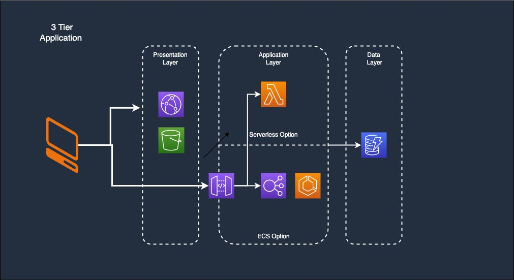
Amazon Redshift just announced the general availability of Multi-AZ deployments for provisioned RA3 clusters that support running your data warehouse in two Availability Zones simultaneously and can continue operating in unforeseen failure scenarios. A Multi-AZ deployment is intended for customers with mission-critical analytics applications that require the highest levels of  resilience and availability.
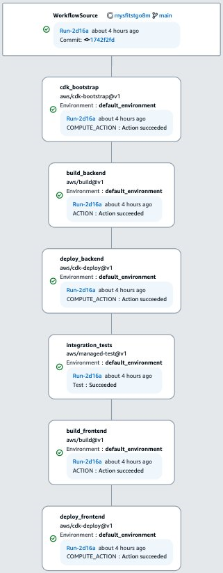
A Redshift Multi-AZ deployment leverages compute resources in two AZs to scale data warehouse workload processing.  In situations where there is a high level or concurrency Redshift will automatically leverage the resources in both AZs to scale the workload for both read and write requests.
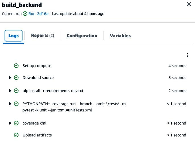
Our pre-launch tests found that Amazon Redshift Multi-AZ deployments reduce recovery time to under 60 seconds or less in the unlikely case of an AZ failure.

Single-AZ vs. Multi-AZ deployment

Amazon Redshift requires a cluster subnet group to create a cluster in your VPC. The cluster subnet group includes information about the VPC ID and a list of subnets in your VPC. When you launch a cluster, Amazon Redshift either creates a default cluster subnet group automatically or you choose a cluster subnet group of your choice so that Amazon Redshift can provision your cluster in one of the subnets in the VPC. You can configure your cluster subnet group to add subnets from different Availability Zones that you want Amazon Redshift to use for cluster deployment.

All Amazon Redshift clusters today are created and situated in a particular Availability Zone within an AWS Region and thus called Single-AZ deployments. For a Single-AZ deployment, Amazon Redshift selects the subnet from one of the Availability Zones within a Region and deploys the cluster there. You can choose an Availability Zone for deployment, and Amazon Redshift will deploy your cluster in the chosen Availability Zone based on the subnets provided.

On the other hand, a multi-AZ deployment is provisioned in two Availability Zones simultaneously. For a Multi-AZ deployment, Amazon Redshift automatically selects two subnets from two different Availability Zones and deploys an equal number of compute nodes in each Availability Zone. All these compute nodes are utilized via a single endpoint as compute nodes from both Availability Zones are used for workload processing.

As shown in the following diagrams, Amazon Redshift deploys a cluster in a single Availability Zone for Single-AZ deployment, and two Availability Zones for Multi-AZ deployment.

Auto recovery of multi-AZ deployment

In the unlikely event of an Availability Zone failure, Amazon Redshift Multi-AZ deployments continue to serve your workloads by automatically using resources in the other Availability Zone. You are not required to make any application changes to maintain business continuity during unforeseen outages since a multi-AZ deployment is accessed as a single data warehouse with one endpoint. Amazon Redshift Multi-AZ deployments are designed to ensure there is no data loss, and you can query all data committed up until the point of failure.

As shown in the below diagram, if there is an unlikely event that causes compute nodes in AZ1 to fail, then a multi-AZ deployment automatically recovers to use compute resources in AZ2. Amazon Redshift will also automatically provision identical compute nodes in another availability zone (AZ3) to continue operating simultaneously in two Availability zones (AZ2 and AZ3).

Amazon Redshift Multi-AZ deployment is not only used for protection against the possibility of Availability Zone failures, but it can also maximize your data warehouse performance by automatically distributing workload processing across two Availability Zones. A Multi-AZ deployment will always process an individual query using compute resources only from one Availability Zone, but it can automatically distribute processing of multiple simultaneous queries to both Availability Zones to increase overall performance for high concurrency workloads.

It’s a good practice to set up automatic retries in your extract, transform, and load (ETL) processes and dashboards so that they can be reissued and served by the cluster in the secondary Availability Zone when an unlikely failure happens in the primary Availability Zone. If a connection is dropped, it can then be retried or reestablished immediately. In addition, queries and loads that were running in the failed Availability Zone will be aborted. New queries issued at or after a failure occurs may experience run delays while the multi-AZ data warehouse is being recovered to a two AZ setup.

Overview of solution

In this post, we provide a walkthrough of how to create and manage a Multi-AZ deployment for Amazon Redshift using the AWS Management Console. We also test the fault tolerance of an Amazon Redshift Multi-AZ data warehouse and monitor queries in your Multi-AZ deployment.

Create a new Multi-AZ deployment from the console

You can easily create a new multi-AZ deployments through Amazon Redshift console. Amazon Redshift will deploy the same number of nodes in each of the two Availability Zones for a Multi-AZ deployment. All nodes of a multi-AZ deployment can perform read and write workload processing during normal operation. A Multi-AZ deployment is supported only for provisioned RA3 clusters.

Follow these steps to create an Amazon Redshift provisioned cluster in two Availability Zones:

  1. On the Amazon Redshift console, in the navigation pane, choose Clusters.
  2. Click on Create cluster.

For general information about creating clusters, see Creating a cluster.

  1. Choose one of the RA3 node types on the Node type drop-down menu. The Multi-AZ deployment option only becomes available when you choose an RA3 node type.
  2. For Multi-AZ deployment, select Multi-AZ option.
  3. For Number of nodes per AZ, enter the number of nodes that you need for your cluster.

  1. Under the Database configurations, choose Admin user name and Admin user password.
  2. Turn Use defaults on next to Additional configurations to modify the default settings.
  3. Under Network and security, specify the following:
    1. For Virtual private cloud (VPC), choose the VPC you want to deploy the cluster in.
    2. For VPC security groups, either leave as default or add the security groups of your choice.
    3. For Cluster subnet group, either leave as default or add a cluster subnet group of your choice. For a Multi-AZ deployment, a cluster subnet group must include one subnet each from at least three or more different Availability Zones.

For general information about managing cluster subnet groups, see Cluster subnet groups

  1. Under Database configuration, for Database port, you either use the default value 5439 or choose a value from the range of 5431–5455 and 8191–8215.
  2. Under Database configuration, in the Database encryption section, to use a custom AWS Key Management Service (AWS KMS) key other than the default KMS key, choose Customize encryption settings. This option is deselected by default.
  3. Under Choose an AWS KMS key, you can either choose an existing KMS key, or choose Create an AWS KMS key to create a new KMS key.

For more information to create key using KMS, refer to Creating keys.

  1. Choose Create cluster.

When the cluster creation succeeds, you can view the details on the cluster details page.

Under General information, you can see Multi-AZ as Yes.

On the Properties tab, under Network and security settings, you can find the details on the primary and secondary Availability Zone.

Create a new Multi-AZ deployment from the CLI

The following create-cluster AWS CLI command shows how to create a Multi-AZ cluster

aws redshift create-cluster 
--port 5439 
    --master-username master
    --master-user-password ######
    --node-type ra3.4xlarge
    --number-of-nodes 2
    --profile maz-test
    --endpoint-url https://redshift.us-east-1.amazonaws.com
    --region eu-west-1
    --cluster-identifier redshift-cluster-1
    --multi-az 
    --maintenance-track-name CURRENT
    --encrypted

Convert a Single-AZ deployment to Multi-AZ deployment

To convert an existing Single-AZ deployment to a Multi-AZ deployment, you can go to the Redshift console and select your Redshift cluster that currently is Single-AZ setup and navigate to Actions and select Activate Multi-AZ. Your Single-AZ cluster must be encrypted for a successful conversion to Multi-AZ. During conversion to Multi-AZ, Redshift will double the total number of nodes distributing them equally in each AZ. Redshift will not allow you to split existing number of nodes while converting to Multi-AZ to maintain consistent query performance.

Complete the following steps to create a Multi-AZ deployment restored from a snapshot:

  1. On the Amazon Redshift console, in the navigation pane, choose Clusters.
  2. Select your cluster and navigate to the cluster details page.
  3. On the Actions menu, choose Activate Multi-AZ.

  1. Review the modification summary and confirm by choosing Activate Multi-AZ.

Using the below AWS CLI command you can convert a single AZ Redshift data warehouse to Multi-AZ.

aws redshift modify-cluster 
    --profile maz-test
    --endpoint-url https://redshift.eu-west-1.amazonaws.com
    --region eu-west-1
    --cluster-identifier redshift-cluster-1
    --multi-az

Convert a Multi-AZ deployment to Single-AZ deployment

Redshift also supports conversion of a Multi-AZ deployment into Single-AZ.  This option provides customers with the flexibility to switch between different deployments with few easy steps as follows:

  1. On the Amazon Redshift console, in the navigation pane, choose Clusters.
  2. Select your cluster and navigate to the cluster details page.
  3. On the Actions menu, choose Deactivate Multi-AZ.

  4. Review the modification summary and confirm by choosing Deactivate Multi-AZ.

Creating a Multi-AZ data warehouse restored from a snapshot

Existing customers can also create a Multi-AZ deployment by restoring a snapshot from an existing Single-AZ deployment. See the required steps as below.

  1. On the Amazon Redshift console, in the navigation pane, choose Clusters.
  2. Select the cluster and navigate to the cluster details page.
  3. Choose the Maintenance
  4. Select a snapshot and choose Restore snapshot, Restore to provisioned cluster.
  5. Review the Cluster configuration and Cluster details values of the new cluster to be created using the snapshot information.
  6. Select Multi-AZ option and update the properties of the new cluster, then choose Restore cluster from snapshot at the bottom of the page.

Resizing a Multi-AZ data warehouse

Redshift Multi-AZ feature also supports resizing Multi-AZ Redshift cluster deployments to change the cluster configuration based on scaling needs. You can change both number and type of nodes as per needs.

  1. On the Amazon Redshift console, in the navigation pane, choose Clusters.
  2. Select your cluster and navigate to the cluster details page.
  3. On the Actions menu, choose
  4. Once selected it will bring into another screen to show cluster resize screen where you can choose type and number of nodes and click on Resize cluster.

Failing over Multi-AZ deployment

In addition to the automatic recovery process, you can also trigger this process manually for your data warehouse using the Failover primary compute option. This approach can be used to manage operational maintenance and other planned operational procedures as per the needs of the respective environment. When the cluster successfully recovers, Multi-AZ deployment becomes available. Your Multi-AZ deployment also automatically provisions new compute nodes in another Availability Zone as soon as it is available.

Let’s manually trigger the Failover of your Redshift Multi-AZ deployment.

  1. On the Amazon Redshift console, choose Clusters in the navigation pane.
  2. Navigate to the cluster detail page
  3. From Actions, choose Failover primary compute.
  4. When prompted, choose Confirm.


After the cluster is back to Available status, you can observe that the primary and secondary Availability Zones have changed.

The following screenshot shows the status before injecting failure.

The following screenshot shows the status after injecting failure.

Restore a table from snapshot

You can restore a single table from a snapshot from your Multi-AZ cluster. When you restore a single table from a snapshot, you specify the source snapshot, database, schema, and table name, and the target database, schema, and a new table name for the restored table.

To restore a table from a snapshot:

  1. On the Amazon Redshift console, in the navigation pane, choose Clusters.
  2. Select your cluster and navigate to the cluster details page.
  3. On the Actions menu, choose Restore table.
  4. Enter the information about which snapshot, source table, and target table to use, and then choose Restore table.

Enable public connections for your Multi-AZ data warehouse

  1. From the navigation menu, choose CLUSTERS.
  2. Choose the Multi-AZ cluster that you want to modify.
  3. Choose Actions.
  4. Choose Turn on Publicly accessible.
  5. Choose Elastic IP address, if you do not choose one, an address will be randomly assigned to you.
  6. Choose Save changes.


Monitor queries for Multi-AZ deployments

A Multi-AZ deployment uses compute resources that are deployed in both Availability Zones and can continue operating in the event that the resources in a given Availability Zone are not available. All the compute resources are used at all times, which allows full operation across two Availability Zones in both read and write operations.

You can query SYS_views in the pg_catalog schema to monitor Multi-AZ query runs. The SYS_views cover query run activities and stats from primary and secondary clusters.

The following are the system tables in the SYS_view list:

Follow these steps to monitor the query run on Multi-AZ deployment from the Amazon Redshift Console:

  1. On the Amazon Redshift console, connect to the database in your Multi-AZ deployment and run queries through the query editor.
  2. Run any sample query on the Multi-AZ Redshift deployment.
  3. For a Multi-AZ deployment, you can identify a query and the Availability Zone where it is being run (running on the primary or secondary availability zone) by using the compute_type column in the SYS_QUERY_HISTORY table. The valid values for the compute type column are as follows:
    1. primary – When run on primary availability zone in the Multi-AZ deployment.
    2. secondary – When run on secondary availability zone in the Multi-AZ deployment.

The following is a sample query using the compute_type column to monitor a query:

dev=# select (compute_type) as compute_type, left(query_text, 50) query_text from sys_query_history order by start_time desc;

 compute_type | query_text
--------------+----------------------------------------------------
 secondary    | select count(*) from t1;
 primary 	   select count(*) from t2;

You can also access the query history from the console to analyze your query diagnostics.

  1. On the Query monitoring tab, choose Connect to database.

  1. For Connection, choose Create a new connection
  2. For Authentication, choose Temporary credentials
  3. For Database name, enter the database name (for example, dev).
  4. For Database user, enter the database user name (for example, awsuser).
  5. Choose Connect.

After you’re connected, under Query Monitoring, on the Query history tab, you can view all the queries and loads, as shown in the following screenshot.

Under Metric filters, you can use the various filters in the Additional filtering options section to view query history based on Time interval, Users, Databases, or SQL commands.

There are a few limitations when working with Amazon Redshift Multi-AZ in preview mode, refer here for the limitations.

Customer feedback

Janssen Pharmaceuticals, a subsidiary of Johnson & Johnson, researches and manufactures medicines with a focus on the changing needs of patients and the healthcare industry.

“Janssen Pharmaceutical uses Amazon Redshift to enable critical insights that drive important business decisions for our data scientists, data stewards, business users, and external stakeholders. With Amazon Redshift Multi-AZ, we can be confident that our data warehouse will always be available without any disruptions that might delay impact our ability to make critical business decisions.”

– Shyam Mohapatra, Director of Information Technology – Janssen Pharmaceutical Companies of Johnson & Johnson

Stripe is a technology company that builds economic infrastructure for the internet. Stripe’s products power payments for online and in-person retailers, subscriptions businesses, software platforms and marketplaces, and everything in between.

“Millions of companies use Stripe’s software and APIs to accept payments, send payouts, and manage their businesses online.  Access to their Stripe data via leading data warehouses like Amazon Redshift has been a top request from our customers. Our customers needed highly available, secure, fast, and integrated analytics at scale without building complex data pipelines or moving and copying data around. With Stripe Data Pipeline for Amazon Redshift, we’re helping our customers set up a direct and reliable data pipeline in a few clicks. 

Stripe Data Pipeline enables our customers to automatically share their complete, up-to-date Stripe data with their Amazon Redshift data warehouse, and take their business analytics and reporting to the next level.”

– Brian Brunner, Senior Manager, Engineering at Stripe

Conclusion

This post demonstrated how to configure an Amazon Redshift Multi-AZ deployment in two Availability Zones and test the fault tolerance of your workloads during an unlikely failure of an Availability Zone. Amazon Redshift Multi-AZ deployment also helps improve overall performance of your data warehouse because compute nodes in both Availability Zones are used for read and write operations. Amazon Redshift Multi-AZ data warehouse helps meet the demands of customers with mission critical analytics applications that require the highest levels of availability and resiliency. For more details, refer Configuring Multi-AZ deployment.


About the Authors

Ranjan Burman is an Analytics Specialist Solutions Architect at AWS. He specializes in Amazon Redshift and helps customers build scalable analytical solutions. He has more than 16 years of experience in different database and data warehousing technologies. He is passionate about automating and solving customer problems with cloud solutions.

Saurav Das is part of the Amazon Redshift Product Management team. He has more than 16 years of experience in working with relational databases technologies and data protection. He has a deep interest in solving customer challenges centered around high availability and disaster recovery.

Anusha Challa is a Senior Analytics Specialist Solutions Architect focused on Amazon Redshift. She has helped many customers build large-scale data warehouse solutions in the cloud and on premises. She is passionate about data analytics and data science.

Nita Shah is an Analytics Specialist Solutions Architect at AWS based out of New York. She has been building data warehouse solutions for over 20 years and specializes in Amazon Redshift. She is focused on helping customers design and build enterprise-scale well-architected analytics and decision support platforms.

Suresh Patnam is a Principal BDM – GTM AI/ML Leader at AWS. He works with customers to build IT strategy, making digital transformation through the cloud more accessible by using data and AI/ML. In his spare time, Suresh enjoys playing tennis and spending time with his family.