Tag Archives: Advanced (300)

Simplify data ingestion from Amazon S3 to Amazon Redshift using auto-copy

Post Syndicated from Jason Pedreza original https://aws.amazon.com/blogs/big-data/simplify-data-ingestion-from-amazon-s3-to-amazon-redshift-using-auto-copy/

Amazon Redshift is a fast, scalable, secure, and fully managed cloud data warehouse that makes it simple and cost-effective to analyze your data using standard SQL and your existing business intelligence (BI) tools. Tens of thousands of customers today rely on Amazon Redshift to analyze exabytes of data and run complex analytical queries, making it the most widely used cloud data warehouse.

Data ingestion is the process of getting data to Amazon Redshift. You can leverage one of the many zero-ETL integration methods to make data available in Amazon Redshift directly. However, if your data is in your Amazon S3 bucket, then you can simply load data from Amazon Simple Storage Service (Amazon S3) to Amazon Redshift using the COPY command. A COPY command is the most efficient way to load a table from S3 because it uses the Amazon Redshift’s massively parallel processing (MPP) architecture to read and load data in parallel.

Amazon Redshift launched auto-copy support to simplify data loading from Amazon S3 into Amazon Redshift. You can now setup continuous file ingestion rules to track your Amazon S3 paths and automatically load new files without the need for additional tools or custom solutions. This also enables end users to have the latest data available in Amazon Redshift shortly after the source data is available.

This post shows you how to build automatic file ingestion pipelines in Amazon Redshift when source files are located on Amazon S3 by using a simple SQL command. In addition, we show you how to enable auto-copy using auto-copy jobs, how to monitor jobs, considerations, and best practices.

Overview of the auto-copy feature in Amazon Redshift

The auto-copy feature in Amazon Redshift leverages the S3 event integration to automatically load data into Amazon Redshift and simplifies automatic data loading from Amazon S3 with a simple SQL command. You can enable Amazon Redshift auto-copy by creating auto-copy jobs. A auto-copy job is a database object that stores, automates, and reuses the COPY statement for newly created files that land in the S3 folder.

The following diagram illustrates this process.

S3 event integration and auto-copy jobs have the following benefits:

  • Users can now load data from Amazon S3 automatically without having to build a pipeline or using an external framework
  • auto-copy jobs offer automatic and incremental data ingestion from an Amazon S3 location without the need to implement a custom solution
  • This functionality comes at no additional cost
  • Existing COPY statements can be converted into auto-copy jobs by appending the JOB CREATE <job_name> parameter
  • It keeps track of loaded files and minimizes data duplication.
  • It can be quickly set up using a simple SQL statement using your choice of JDBC/ODBC clients.
  • It has automatic error handling of bad quality data files.
  • It has a mechanism to load-once for each file. This means that there is no need to generate explicit manifest files.

Prerequisites

To get started with auto-copy, you need the following prerequisites:

  • An AWS account
  • An encrypted Amazon Redshift provisioned cluster or Amazon redshift serverless workgroup
  • An Amazon S3 bucket
  • Add following to the Amazon S3 bucket policy
    {
        "Version": "2012-10-17",
        "Statement": [
            {
                "Sid": "Auto-Copy-Policy-01",
                "Effect": "Allow",
                "Principal": {
                    "Service":"redshift.amazonaws.com"
                        
                    
                },
                "Action": [
                    "s3:GetBucketNotification",
                    "s3:PutBucketNotification",
                    "s3:GetBucketLocation"
                ],
                "Resource": "arn:aws:s3:::<<your-s3-bucket-name>>",
                "Condition": {
                    "StringEquals": {
                        "aws:SourceArn": "arn:aws:redshift:<region-name>:<aws-account-id>:integration:*",
                        "aws:SourceAccount": "<aws-account-id>"
                    }
                }
            }
        ]
    }

Set up Amazon S3 event Integration

An Amazon S3 event integration facilitates seamless and automated data ingestion from S3 buckets into an Amazon Redshift data warehouse, streamlining the process of transferring and storing data for analytical purposes

  1. Sign in to the AWS Management Console and Navigate to Amazon Redshift home page. Under Integrations section choose S3 event integrations

  2. Choose Create S3 event integration

  3. Enter Integration name and Description, choose Next

  4. Choose Browse S3 buckets, a dialog box pops up, select the Amazon S3 bucket and choose Continue

  5. Amazon S3 bucket is selected. Choose Next
  6. Choose Browse Redshift data warehouse

  7. Choose the Amazon Redshift data warehouse and choose Continue

  8. Then Amazon Redshift resource policy needs access to S3 event integration. In case of Resource policy error, check Fix it for me and choose Next

  9. Add Tags as required and choose Next

  10. Review changes and choose Create S3 event integration
  11. An S3 event integration is created. Wait until the status of S3 event integration is Active

Set up auto-copy jobs

In this section, we demonstrate how to automate data loading of files from Amazon S3 into Amazon Redshift. With the existing COPY syntax, we add the JOB CREATE parameter to perform a one-time setup for automatic file ingestion. See the following code:

COPY <table-name>
FROM 's3://<s3-object-path>'
[COPY PARAMETERS...]
JOB CREATE <job-name> [AUTO ON | OFF];

Auto ingestion is enabled by default on auto-copy jobs. Files already present at the S3 location will not be visible to the auto-copy job. Only files added after JOB creation are tracked by Amazon Redshift.

Automate ingestion from a single data source

With a auto-copy job, you can automate ingestion from a single data source by creating one job and specifying the path to the S3 objects that contain the data. The S3 object path can reference a set of folders that have the same key prefix.

In this example, we have multiple files that are being loaded on a daily basis containing the sales transactions across all the stores in the US. For this we can create a store_sales folder in the bucket.

The following code creates the store_sales table:

DROP TABLE IF EXISTS public.store_sales;
CREATE TABLE IF NOT EXISTS public.store_sales
(
  ss_sold_date_sk int4,            
  ss_sold_time_sk int4,     
  ss_item_sk int4 not null,      
  ss_customer_sk int4,           
  ss_cdemo_sk int4,              
  ss_hdemo_sk int4,         
  ss_addr_sk int4,               
  ss_store_sk int4,           
  ss_promo_sk int4,           
  ss_ticket_number int8 not null,        
  ss_quantity int4,           
  ss_wholesale_cost numeric(7,2),          
  ss_list_price numeric(7,2),              
  ss_sales_price numeric(7,2),
  ss_ext_discount_amt numeric(7,2),             
  ss_ext_sales_price numeric(7,2),              
  ss_ext_wholesale_cost numeric(7,2),           
  ss_ext_list_price numeric(7,2),               
  ss_ext_tax numeric(7,2),                 
  ss_coupon_amt numeric(7,2), 
  ss_net_paid numeric(7,2),   
  ss_net_paid_inc_tax numeric(7,2),             
  ss_net_profit numeric(7,2),
  primary key (ss_item_sk, ss_ticket_number)
 ) 
DISTKEY (ss_item_sk) 
SORTKEY (ss_sold_date_sk);

Next, we create the auto-copy job to automatically load the gzip-compressed files into the store_sales table:

COPY store_sales
FROM 's3://aws-redshift-s3-auto-copy-demo/store_sales'
IAM_ROLE 'arn:aws:iam::**********:role/Redshift-S3'
gzip delimiter '|' EMPTYASNULL
region 'us-east-1'
JOB CREATE job_store_sales AUTO ON;

Each day’s sales transactions are loaded to their own folder in Amazon S3.

Now upload the files for transaction sold on 2002-12-31. Each folder contains multiple gzip-compressed files.

Since the auto-copy job is already created, it automatically loads the gzip-compressed files located in the S3 object path specified in the COPY command to the store_sales table.

Let’s run a query to get the daily total of sales transactions across all the stores in the US:

SELECT ss_sold_date_sk, count(1)
  FROM store_sales
GROUP BY ss_sold_date_sk;

The output shown comes from the transactions sold on 2002-12-31.

The following day, incremental sales transactions data are loaded to a new folder in the same S3 object path.

As new files arrive to the same S3 object path, the auto-copy job automatically loads the unprocessed files to the store_sales table in an incremental fashion.

All new sales transactions for 2003-01-01 are automatically ingested, which can be verified by running the following query:

SELECT ss_sold_date_sk, count(1)
  FROM store_sales
GROUP BY ss_sold_date_sk;

Automate ingestion from multiple data sources

We can also load an Amazon Redshift table from multiple data sources. When using a pub/sub pattern where multiple S3 buckets populate data to an Amazon Redshift table, you have to maintain multiple data pipelines for each source/target combination. With new parameters in the COPY command, this can be automated to handle data loads efficiently.

In the following example, the Customer_1 folder has Green Cab Company sales data, and the Customer_2 folder has Red Cab Company sales data. We can use the COPY command with the JOB parameter to automate this ingestion process.

The following screenshot shows sample data stored in files. Each folder has similar data but for different customers.

The target for these files in this example is the Amazon Redshift table cab_sales_data.

Define the target table cab_sales_data:

DROP TABLE IF EXISTS cab_sales_data;
CREATE TABLE IF NOT EXISTS cab_sales_data
(
  vendorid                VARCHAR(4),
  pickup_datetime         TIMESTAMP,
  dropoff_datetime        TIMESTAMP,
  store_and_fwd_flag      VARCHAR(1),
  ratecode                INT,
  pickup_longitude        FLOAT4,
  pickup_latitude         FLOAT4,
  dropoff_longitude       FLOAT4,
  dropoff_latitude        FLOAT4,
  passenger_count         INT,
  trip_distance           FLOAT4,
  fare_amount             FLOAT4,
  extra                   FLOAT4,
  mta_tax                 FLOAT4,
  tip_amount              FLOAT4,
  tolls_amount            FLOAT4,
  ehail_fee               FLOAT4,
  improvement_surcharge   FLOAT4,
  total_amount            FLOAT4,
  payment_type            VARCHAR(4),
  trip_type               VARCHAR(4)
)
DISTSTYLE EVEN
SORTKEY (passenger_count,pickup_datetime);

You can define two auto-copy jobs as shown in the following code to handle and monitor the ingestion of sales data belonging to different customers, in our case Customer_1 and Customer_2. These jobs monitor the Customer_1 and Customer_2 folders and load new files that are added here.

COPY public.cab_sales_data
FROM 's3://aws-redshift-s3-auto-copy-demo/Customer_1'
IAM_ROLE 'arn:aws:iam::**********:role/Redshift-S3'
DATEFORMAT 'auto'
IGNOREHEADER 1
DELIMITER ','
IGNOREBLANKLINES
REGION 'us-east-1'
JOB CREATE job_green_cab AUTO ON;

COPY public.cab_sales_data
FROM 's3:// aws-redshift-s3-auto-copy-demo/Customer_2'
IAM_ROLE 'arn:aws:iam::**********:role/Redshift-S3'
DATEFORMAT 'auto'
IGNOREHEADER 1
DELIMITER ','
IGNOREBLANKLINES
REGION 'us-east-1'
JOB CREATE job_red_cab AUTO ON;

After setting up the two jobs, we can upload the relevant files into their respective folders. This will make sure that the data is loaded efficiently as soon as the files arrive. Each customer is assigned its own vendorid, as shown in the following output:

SELECT vendorid,
       sum(passenger_count) as total_passengers 
  FROM cab_sales_data
GROUP BY vendorid;

result 1

Manually run a auto-copy job

There might be scenarios wherein the auto-copy job needs to be paused, meaning it needs to stop looking for new files, for example, to fix a corrupted data pipeline at the data source.

In that case, either use the auto-copy job ALTER command to set AUTO to OFF or create a new auto-copy job with AUTO OFF. Once this is set, auto copy will no longer look for new files.

If necessary, users can manually invoke auto-copy job which will do the work and ingest if new files are found.

auto-copy job RUN <auto-copy job Name>

You can disable “AUTO ON” in the existing auto-copy job using the following command:

auto-copy job ALTER <auto-copy job Name> AUTO OFF

The following table compares the syntax and data duplication between a regular copy statement and the new auto-copy job

. Copy Auto-copy job
Syntax COPY <table-name>
FROM 's3://<s3-object-path>'
[COPY PARAMETERS...]
COPY <table-name>
FROM 's3://<s3-object-path>'
[COPY PARAMETERS...]
JOB CREATE <job-name>;
Data Duplication If it is run multiple times against the same S3 folder, it will load the data again, resulting in data duplication. It will not load the same file twice, preventing data duplication.

Error handling and monitoring for auto-copy jobs

auto-copy jobs continuously monitor the S3 folder specified during job creation and perform ingestion whenever new files are created. New files created under the S3 folder are loaded exactly once to avoid data duplication.

By default, if there are data or format issues with the specific files, the auto-copy job will fail to ingest the files with a load error and log details to the system tables. The auto-copy job will remain AUTO ON with new data files and will continue to ignore previously failed files.

Amazon Redshift provides the following system tables for users to monitor or troubleshoot auto-copy jobs as needed:

  • List auto-copy jobs – Use SYS_COPY_JOB to list the auto-copy jobs stored in the database:
SELECT * 
  FROM sys_copy_job;

  • Get a summary of a auto-copy job – Use the SYS_LOAD_HISTORY view to get the aggregate metrics of a auto-copy job operation by specifying the copy_job_id. It shows the aggregate metrics of the files that have been processed by a auto-copy job.
SELECT *
  FROM sys_load_history
 WHERE copy_job_id = 274978;

  • Get details of a auto-copy job – Use STL_LOAD_COMMITS to get the status and details of each file that was processed by a auto-copy job:

SELECT *
  FROM stl_load_commits
 WHERE copy_job_id = 274978
ORDER BY curtime ASC;

  • Get exception details of a auto-copy job – Use STL_LOAD_ERRORS to get the details of files that failed to ingest from a auto-copy job:
SELECT   query,
    slice,
    starttime , 
    filename,
    line_number,
    colname,
    type,
    err_code,
    err_reason,
    copy_job_id,
    raw_line,
    raw_field_value
  FROM stl_load_errors
 WHERE copy_job_id = 274978;

Auto-copy job best practices

In an auto-copy job, when a new file is detected and ingested (automatically or manually), Amazon Redshift stores the file name and doesn’t run this specific job when a new file is created with the same file name.

The following are the recommended best practices when working with files using the auto-copy job:

  • Use unique file names for each file in a auto-copy job (for example, 2022-10-15-batch-1.csv). However, you can use the same file name as long as it’s from different auto-copy jobs:
    • job_customerA_sales – s3://redshift-blogs/sales/customerA/2022-10-15-sales.csv
    • job_customerB_sales – s3://redshift-blogs/sales/customerB/2022-10-15-sales.csv
  • Do not update file contents. Do not overwrite existing files. Changes in existing files will not be reflected to the target table. The auto-copy job doesn’t pick up updated or overwritten files, so make sure they’re renamed as new file names for the auto-copy job to pick up.
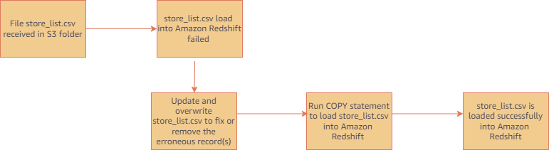
  • Run regular COPY statements (not a job) if you need to ingest a file that was already processed by your auto-copy job. (COPY statement without a JOB CREATE syntax doesn’t track loaded files.) For example, this is helpful in scenarios where you don’t have control of the file name and the initial file received failed. The following figure shows a typical workflow in this case.
  • Delete and recreate your auto-copy job if you want to reset file tracking history and start over. You can drop auto-copy job using following command.
    auto-copy job DROP <auto-copy job Name>

auto-copy job considerations

Here are the main things to consider when using auto-copy:

For additional details on other considerations for auto-copy, refer to the AWS documentation.

Customer feedback

GE Aerospace is a global provider of jet engines, components, and systems for commercial and military aircraft. The company has been designing, developing, and manufacturing jet engines since World War I.

“GE Aerospace uses AWS analytics and Amazon Redshift to enable critical business insights that drive important business decisions. With the support for auto-copy from Amazon S3, we can build simpler data pipelines to move data from Amazon S3 to Amazon Redshift. This accelerates our data product teams’ ability to access data and deliver insights to end users. We spend more time adding value through data and less time on integrations.”

– Alcuin Weidus Sr Principal Data Architect at GE Aerospace

Conclusion

This post demonstrated how to automate data ingestion from Amazon S3 to Amazon Redshift using the auto-copy feature. This new functionality helps make Amazon Redshift data ingestion easier than ever, and will allow SQL users to get access to the most recent data using a simple SQL command.

Users can begin ingesting data to Redshift from Amazon S3 with simple SQL commands and gain access to the most up-to-date data without the need for third-party tools or custom implementation.


About the authors

Tahir Aziz is an Analytics Solution Architect at AWS. He has worked with building data warehouses and big data solutions for over 15+ years. He loves to help customers design end-to-end analytics solutions on AWS. Outside of work, he enjoys traveling and cooking.

Omama Khurshid is an Acceleration Lab Solutions Architect at Amazon Web Services. She focuses on helping customers across various industries build reliable, scalable, and efficient solutions. Outside of work, she enjoys spending time with her family, watching movies, listening to music, and learning new technologies.

Raza Hafeez is a Senior Product Manager at Amazon Redshift. He has over 13 years of professional experience building and optimizing enterprise data warehouses and is passionate about enabling customers to realize the power of their data. He specializes in migrating enterprise data warehouses to AWS Modern Data Architecture.

Jason Pedreza is an Analytics Specialist Solutions Architect at AWS with data warehousing experience handling petabytes of data. Prior to AWS, he built data warehouse solutions at Amazon.com. He specializes in Amazon Redshift and helps customers build scalable analytic solutions.

Nita Shah is an Analytics Specialist Solutions Architect at AWS based out of New York. She has been building data warehouse solutions for over 20 years and specializes in Amazon Redshift. She is focused on helping customers design and build enterprise-scale well-architected analytics and decision support platforms.

Eren Baydemir, a Technical Product Manager at AWS, has 15 years of experience in building customer-facing products and is currently focusing on data lake and file ingestion topics in the Amazon Redshift team. He was the CEO and co-founder of DataRow, which was acquired by Amazon in 2020.

Eesha Kumar is an Analytics Solutions Architect with AWS. He works with customers to realize the business value of data by helping them build solutions using the AWS platform and tools.

Satish Sathiya is a Senior Product Engineer at Amazon Redshift. He is an avid big data enthusiast who collaborates with customers around the globe to achieve success and meet their data warehousing and data lake architecture needs.

 Hangjian Yuan is a Software Development Engineer at Amazon Redshift. He’s passionate about analytical databases and focuses on delivering cutting-edge streaming experiences for customers.

Enable federation to Amazon QuickSight with automatic provisioning of users between AWS IAM Identity Center and Microsoft Azure AD

Post Syndicated from Aditya Ravikumar original https://aws.amazon.com/blogs/big-data/enable-federation-to-amazon-quicksight-with-automatic-provisioning-of-users-between-aws-iam-identity-center-and-microsoft-azure-ad/

Organizations are working towards centralizing their identity and access strategy across all their applications, including on-premises, third-party, and applications on AWS. Many organizations use identity providers (IdPs) based on OIDC or SAML-based protocols like Microsoft Azure Active Directory (Azure AD) and manage user authentication along with authorization centrally. This authorizes users to access Amazon QuickSight assets-analyses, dashboards, folders, and datasets-through centrally managed Azure AD and AWS IAM Identity Center (successor to AWS Single Sign-On).

IAM Identity Center is an authentication process that allows users to sign into multiple applications with a single set of usernames and passwords. IAM Identity Center makes it easy to centrally manage access to multiple AWS accounts and business applications. It provides your workforce with single sign-on (SSO) access to all assigned accounts and applications from one place.

In this post, we walk you through the steps required to configure federated SSO along with automated email sync between QuickSight and Azure AD via IAM Identity Center. We also demonstrate ways System for Cross-domain Identity Management (SCIM) keeps your IAM Identity Center identities in sync with identities from your IdP.

Solution overview

The following is the reference architecture for configuring IAM Identity Center with Azure AD for automated federation to QuickSight and the AWS Management Console.

The following are the steps involved to set up federated SSO from Azure to QuickSight:

  1. Configure Azure as an IdP in IAM Identity Center.
  2. Register an IAM Identity Center application in Azure AD.
  3. Configure the application in Azure AD.
  4. Enable automatic provisioning of users and groups.
  5. Enable email syncing for federated users in QuickSight console.
  6. Create a QuickSight application in IAM Identity Center.
  7. Add the IAM Identity Center application as a SAML IdP.
  8. Configure AWS Identity and Access Management (IAM) policies and roles.
  9. Configure attribute mappings in IAM Identity Center.
  10. Validate federation to QuickSight from IAM Identity Center.

Prerequisites

To complete this walkthrough, you must have the following prerequisites:

  • An Azure AD subscription with Administrator permission.
  • QuickSight account subscription with Administrator permission.
  • IAM Administrator account.
  • IAM Identity Center Administrator account.

Configure Azure as IdP in IAM Identity Center

To configure Azure as an IdP, complete the following steps:

  1. On the IAM Identity Center console, choose Enable.
    choose Enable
  2. Choose Choose your identity source.
    Choose your identity source.
  3. Select External identity provider to manage all users and groups.
  4. Choose Next.
    Choose Next.
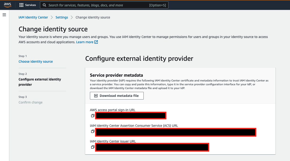
  5. In the Configure external identity provider section, download the service provider metadata file.
  6. Save the AWS access portal sign-in URL, IAM Identity Center Assertion Consumer Service (ACS) URL, and IAM Identity Center issuer URL.
    These are used later in this post.
  7. Leave this tab open in your browser while proceeding to the next steps.

Register an IAM Identity Center application in Azure AD

To register an IAM Identity Center application in Azure AD, complete the following steps:

  1. Sign in to your Azure portal using an administrator account.
  2. Under Azure Services, choose Azure AD and under Manage, choose Enterprise applications.
    Under Azure Services, choose Azure AD and under Manage, choose Enterprise applications.
  3. Choose New application.
  4. Choose Create your own application.
  5. Enter a name for the application.
  6. Select the option Integrate any other application you don’t find in the gallery (Non-gallery).
  7. Choose Create.
    Choose Create.

Configure the application in Azure AD

To configure your application, complete the following steps:

  1. Under Enterprise applications, choose All applications and select the application created in the previous step.
  2. Under Manage, choose Single Sign-on.
  3. Choose SAML.
    Choose SAML.
  4. Choose Single Sign-on to set up SSO with SAML.
  5. Choose Upload metadata file, and upload the file you downloaded from IAM Identity Center.
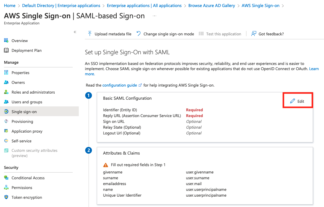
  6. Choose Edit to edit the Basic SAML Configuration section.
    6. Choose Edit to edit the Basic SAML Configuration section.
  • For Identifier (Entity ID), enter the IAM Identity Center issuer URL.
  • For Reply URL (Assertion Consumer Service URL), enter the IAM Identity Center ACS URL.
  1. Under SAML Signing Certificate, choose Download next to Federation Metadata XML.
    7. Under SAML Signing Certificate, choose Download next to Federation Metadata XML.

We use this XML document in later steps when setting up the SAML provider in IAM and in IAM Identity Center.

  1. Leave this tab open in your browser while moving to the next steps.
  2. Switch to the IAM Identity Center tab to complete its setup.
  3. Under Identity provider metadata, choose IdP SAML metadata and upload the federation metadata XML file you downloaded.
    10. Under Identity provider metadata, choose IdP SAML metadata and upload the federation metadata XML file you downloaded.
  4. Review and confirm the changes.
    11. Review and confirm the changes.

Enable automatic provisioning of users and groups

IAM Identity Center supports System for Cross-domain Identity Management (SCIM) v2.0 standard. SCIM keeps your IAM Identity Center identities in sync with external IdPs. This includes any provisioning, updates, and deprovisioning of users between IdP and IAM Identity Center. To enable SCIM, complete the following steps:

  1. On the IAM Identity Center console, choose Settings in the navigation pane.
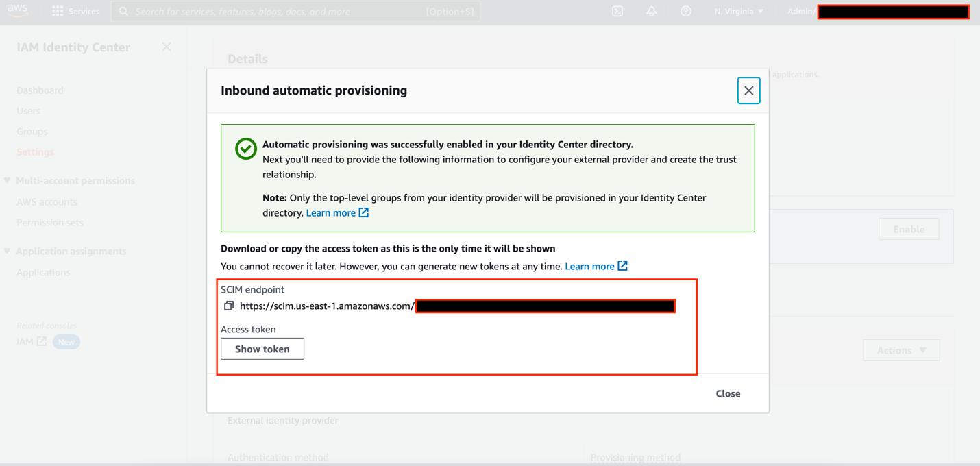
  2. Next to Automatic provisioning, choose Enable.
    2. Next to Automatic provisioning, choose Enable.
  3. Copy the SCIM endpoint and Access token.
    Copy the SCIM endpoint and Access token.
  4. Switch to the Azure AD tab.
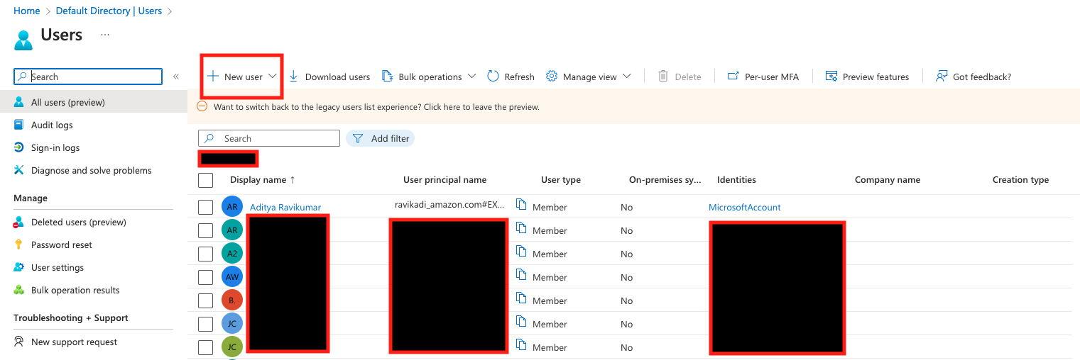
  5. On the Default Directory Overview page, under Manage, choose Users.
    5. On the Default Directory Overview page, under Manage, choose Users.
  6. Choose New user and Create new user(s).
    Make sure the user profile has valid information under First name, Last name, and Email attribute.
    Make sure the user profile has valid information under First name, Last name, and Email attribute.
  7. Under Enterprise applications, choose All applications and select the application you created earlier.
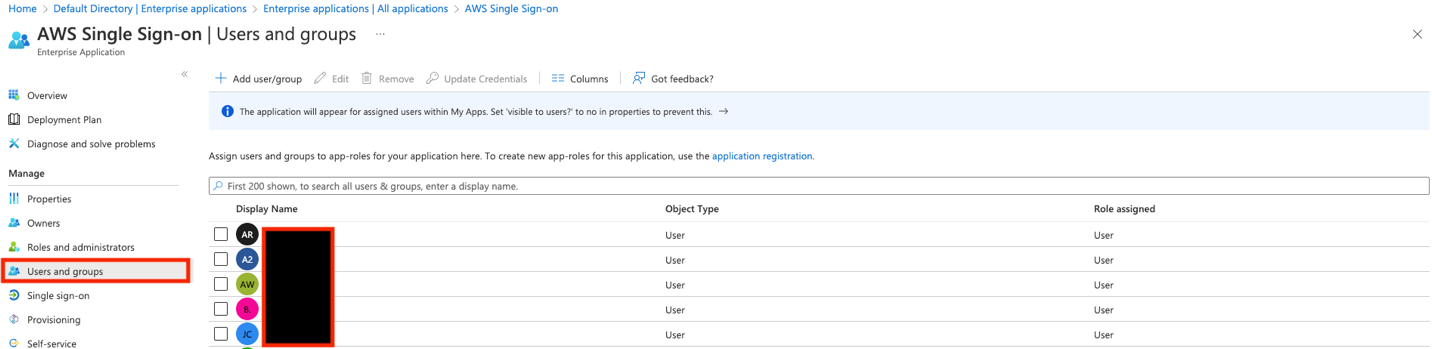
  8. Under Manage, choose Users and groups.
    8. Under Manage, choose Users and groups.
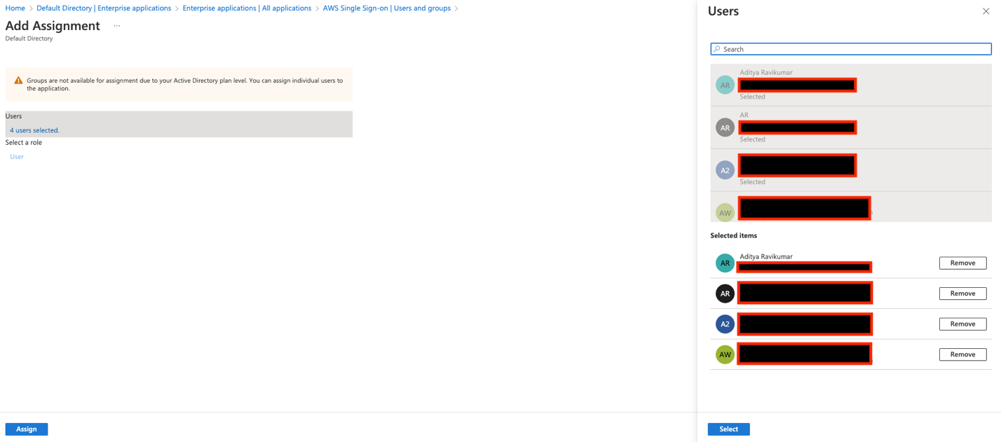
  9. Choose Add user/group, and select the users you created earlier.
  10. Choose Assign.
    Choose Assign.
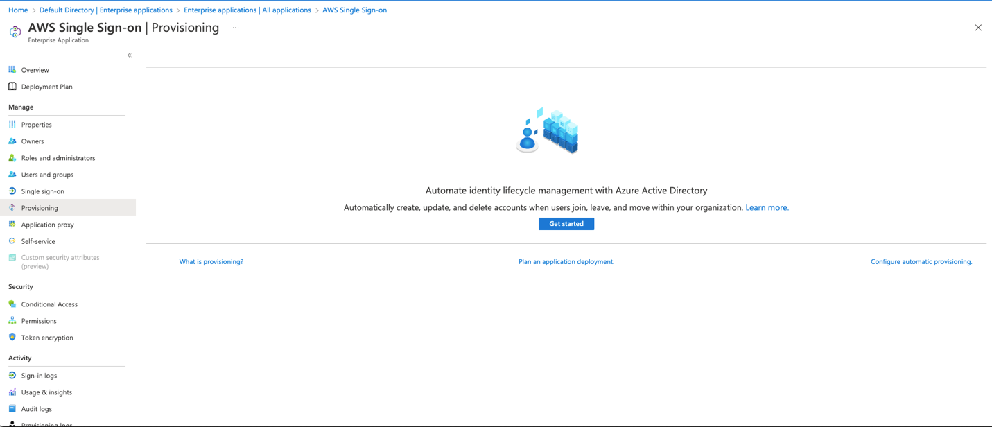
  11. Under Manage, choose Provisioning and Get started.
    11. Under Manage, choose Provisioning and Get started.
  12. Choose Provisioning Mode as Automatic.
  13. For Tenant URL, enter the SCIM endpoint.
  14. For Secret Token, enter the Access token.
  15. Choose Test Connection and Save.
    15. Choose Test Connection and Save.
  16. Under Provisioning, choose Start provisioning.
    16. Under Provisioning, choose Start provisioning.

Make sure the user profile has valid information under First name, Last name, and Email attribute. This is the key value for email sync with QuickSight.

On the IAM Identity Center console, under Users, you can now see all the users provisioned from Azure AD.

Enable email syncing for federated users in QuickSight console

Complete the following steps to enable email syncing for federated users:

  1. Sign in as an admin user to the QuickSight console and choose Manage QuickSight from the user name menu.
    1. Sign in as an admin user to the QuickSight console and choose Manage QuickSight from the user name menu.
  2. Choose Single sign-on (SSO) in the navigation pane.
    2. Choose Single sign-on (SSO) in the navigation pane.
  3. Under Email Syncing for Federated Users, select ON.
    3. Under Email Syncing for Federated Users, select ON.

Create a QuickSight application in IAM Identity Center

Complete the following steps to create a custom SAML 2.0 application in IAM Identity Center.

  1. On the IAM Identity Center console, choose Applications in the navigation pane.
  2. Choose Add application.
    2Choose Add application.
  3. Under Preintegrated applications, search for and choose Amazon QuickSight.
  4. Choose Next.
    Choose Next.
  5. For Display name, enter a name, such as Amazon QuickSight.
  6. For Description, enter a description.
  7. Download the IAM Identity Center SAML metadata file to use later in this post.
  8. For Application start URL, leave as is.
  9. For Relay state, enter https://quicksight.aws.amazon.com.
  10. For Session duration, choose your session duration. The recommended value is 8 hours.
  11. For Application ACS URL, enter https://signin.aws.amazon.com/saml.
  12. For Application SAML audience, enter urn:amazon:webservices.
  13. Choose Submit
    After your settings are saved, your application configuration should look similar to the following screenshot.
    After your settings are saved, your application configuration should look similar to the following screenshot.

You can now assign your users to this application, so that the application appears in their IAM Identity Center portal after login.

  1. On the application page, under Assigned users, choose Assign Users.
    14. On the application page, under Assigned users, choose Assign Users.
  2. Select your users.
  3. Optionally, if you want to enable multiple users in your organization to use QuickSight, the fastest and easiest way is to use IAM Identity Center groups.
  4. Choose Assign Users.
    17. Choose Assign Users.

Add the IAM Identity Center application as a SAML IdP

Complete the following steps to configure IAM Identity Center as your SAML IdP:

  1. Open a new tab in your browser.
  2. Sign in to the IAM console in your AWS account with admin permissions.
  3. Choose Identity providers in the navigation pane.
  4. Choose Add provider.
  5. Select SAML for Provider type.
  6. For Provider name, enter IAM_Identity_Center.
  7. Choose Choose File to upload the metadata document you downloaded earlier from the Amazon QuickSight application.
  8. Choose Add Provider.
    8. Choose Add Provider
  9. On the summary page, record the value for the provider ARN (arn:aws:iam::<AccountID>:saml-provider/IAM_Identity_Center).

You will use this ARN while configuring claims rules later in this post.

Configure IAM policies

In this step, you create three IAM policies for different role permissions in QuickSight:

  • QuickSight-Federated-Admin
  • QuickSight-Federated-Author
  • QuickSight-Federated-Reader

Use the following steps to set up QuickSight-Federated-Admin policy. This policy grants admin privileges in QuickSight to the federated user:

  1. On the IAM console, choose Policies in the navigation pane
  2. Choose Create policy.
  3. Choose JSON and replace the existing text with the following code:

    {
        "Statement": [
            {
                "Action": [
                    "quicksight:CreateAdmin"
                ],
                "Effect": "Allow",
                "Resource": [
                    "arn:aws:quicksight::<yourAWSAccountID>:user/${aws:userid}"
                ]
            }
        ],
        "Version": "2012-10-17"
    }

Ignore the “Missing ARN Region: Add a Region to the quicksight resource ARN” error and continue. Optionally, you could also add a specific AWS region in the ARN.

  1. Choose Review policy
  2. For Name enter QuickSight-Federated-Admin.
  3. Choose Create policy.
  4. Repeat these steps to create the QuickSight-Federated-Author policy using the following JSON code to grant author privileges in QuickSight to the federated user:
    {
        "Statement": [
            {
                "Action": [
                    "quicksight:CreateUser"
                ],
                "Effect": "Allow",
                "Resource": [
                    "arn:aws:quicksight::<yourAWSAccountID>:user/${aws:userid}"
                ]
            }
        ],
        "Version": "2012-10-17"
    }

Ignore the “Missing ARN Region: Add a Region to the quicksight resource ARN” error and continue. Optionally, you could also add a specific AWS region in the ARN.

  1. Repeat these steps to create the QuickSight-Federated-Reader policy using the following JSON code to grant reader privileges in QuickSight to the federated user:
    {
        "Statement": [
            {
                "Action": [
                    "quicksight:CreateReader"
                ],
                "Effect": "Allow",
                "Resource": [
                    "arn:aws:quicksight::<yourAWSAccountID>:user/${aws:userid}"
                ]
            }
        ],
        "Version": "2012-10-17"
    }

Ignore the “Missing ARN Region: Add a Region to the quicksight resource ARN” error and continue. Optionally, you could also add a specific AWS region in the ARN.

Configure IAM roles

Next, create roles that your Azure AD and IAM Identity Center users assume when federating into QuickSight. The following steps set up the admin role:

  1. On the IAM console, choose Roles in the navigation pane.
  2. Choose Create role.
  3. For Select type of trusted entity, choose SAML 2.0 federation.
  4. For SAML provider, choose the provider you created earlier (IAM_Identity_Center).
  5. Select Allow programmatic and AWS Management Console access.
  6. For Attribute, make sure SAML:aud is selected.
  7. For Value, make sure https://signin.aws.amazon.com/saml is selected.
  8. Choose Next.
    Choose Next.
  9. Choose the QuickSight-Federated-Admin IAM policy you created earlier.
  10. Choose Next: Tags.
  11. Choose Next: Review.
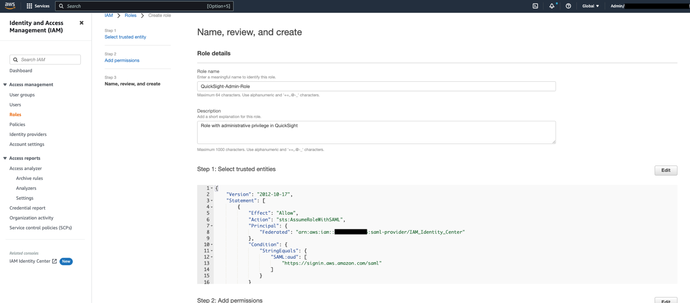
  12. For Role name, enter QuickSight-Admin-Role.
  13. For Role description, enter a description.
    13. For Role description, enter a description.
  14. Choose Create role.
  15. On the IAM console, in the navigation pane, choose Roles.
  16. Choose the QuickSight-Admin-Role role you created to open the role’s properties.
  17. Record the role ARN to use later.
  18. On the Trust relationships tab, choose Edit trust policy.
    18. On the Trust relationships tab, choose Edit trust policy.
  19. For the policy details, enter the following JSON:
    {
        "Version": "2012-10-17",
         "Statement": [
     {
        "Effect": "Allow",
        "Principal": {
    "Federated": "arn:aws:iam::<yourAWSAccountID>:saml-provider/IAM_Identity_Center"
                            },
                "Action": "sts:AssumeRoleWithSAML",
                "Condition": {
                    "StringEquals": {
                        "SAML:aud": "https://signin.aws.amazon.com/saml"	
               }
                }
            },
            {	
                		"Effect": "Allow",
                		"Principal": {
                    	 "Federated":"arn:aws:iam::<yourAWSAccountID>:saml-provider/IAM_Identity_Center"
                				},
                		  "Action": "sts:TagSession",
                   "Condition": {
                    	  "StringLike": {
                       "aws:RequestTag/Email": "*"
               }
                }
            }
        ]
    }

  20. Choose Update Policy.
  21. Repeat these steps to create the roles QuickSight-Author-Role and QuickSight-Reader-Role. Attach the QuickSight-Federated-Author and QuickSight-Federated-Reader policies to their respectively roles.

Configure attribute mappings in IAM Identity Center

The final step is to configure the attribute mappings in IAM Identity Center. The attributes you map here become part of the SAML assertion that is sent to the QuickSight application. You can choose which user attributes in your application map to corresponding user attributes in your connected directory. For more information, refer to Attribute mappings.

  1. On IAM Identity Center console, choose Applications in the navigation pane.
    1. On IAM Identity Center console, choose Applications in the navigation pane.
  2. Select the Amazon QuickSight application you created earlier.
    2. Select the Amazon QuickSight application you created earlier.
  3. On the Actions menu, choose Edit attribute mappings.
  4. Configure the following mappings:
User attribute in the application Maps to this string value or user attribute in IAM Identity Center Format
Subject ${user:email} emailAddress
https://aws.amazon.com/SAML/Attributes/Role arn:aws:iam:: <YourAWSAccount ID>:saml-provider/IAM_Identity_Center, arn:aws:iam:: <YourAWSAccount ID>:role/QuickSight-Admin-Role unspecified
https://aws.amazon.com/SAML/Attributes/RoleSessionName ${user:email} unspecified
https://aws.amazon.com/SAML/Attributes/PrincipalTag:Email ${user:email} url
  1. Choose Save changes.
    Choose Save changes

Validate federation to QuickSight from IAM Identity Center

On the IAM Identity Center console, note down the user portal URL available on the Settings page. We suggest you log out of your AWS account first, or open an incognito browser window. Navigate to the user portal URL, sign in with the credentials of an AD user, and choose your QuickSight application.

On the IAM Identity Center console, note down the user portal URL available on the Settings page.

Navigate to the user portal URL, sign in with the credentials of an AD user, and choose your QuickSight application.

You’re automatically redirected to the QuickSight console.

You’re automatically redirected to the QuickSight console.

You’re automatically redirected to the QuickSight console.

Summary

This post provided step-by-step instructions to configure federated SSO with Azure AD as IdP through IAM Identity Center. We also discussed how SCIM keeps your IAM Identity Center identities in sync with identities from your IdP. This includes any provisioning, updating, and deprovisioning of users between your IdP and IAM Identity Center.

If you have any questions or feedback, please leave a comment.

For additional discussions and help getting answers to your questions, check out the QuickSight Community.


About the author

Aditya Ravikumar is a Solutions Architect at Amazon Web Services. He is based in Seattle, USA. Aditya’s core interests include software development, databases, data analytics and machine learning. He works with AWS customers/partners to provide guidance and technical assistance to transform their business through innovative use of cloud technologies.

Srikanth Baheti is a Specialized World Wide Sr. Solution Architect for Amazon QuickSight. He started his career as a consultant and worked for multiple private and government organizations. Later he worked for PerkinElmer Health and Sciences & eResearch Technology Inc, where he was responsible for designing and developing high traffic web applications, highly scalable and maintainable data pipelines for reporting platforms using AWS services and Serverless computing.

Raji Sivasubramaniam is a Sr. Solutions Architect at AWS, focusing on Analytics. Raji is specialized in architecting end-to-end Enterprise Data Management, Business Intelligence and Analytics solutions for Fortune 500 and Fortune 100 companies across the globe. She has in-depth experience in integrated healthcare data and analytics with wide variety of healthcare datasets including managed market, physician targeting and patient analytics.

Perform multi-cloud analytics using Amazon QuickSight, Amazon Athena Federated Query, and Microsoft Azure Synapse

Post Syndicated from Harish Rajagopalan original https://aws.amazon.com/blogs/big-data/perform-multi-cloud-analytics-using-amazon-quicksight-amazon-athena-federated-query-and-microsoft-azure-synapse/

In this post, we show how to use Amazon QuickSight and Amazon Athena Federated Query to build dashboards and visualizations on data that is stored in Microsoft Azure Synapse databases.

Organizations today use data stores that are best suited for the applications they build. Additionally, they may also continue to use some of their legacy data stores as they modernize and migrate to the cloud. These disparate data stores might be spread across on-premises data centers and different cloud providers. This presents a challenge for analysts to be able to access, visualize, and derive insights from the disparate data stores.

QuickSight is a fast, cloud-powered business analytics service that enables employees within an organization to build visualizations, perform ad hoc analysis, and quickly get business insights from their data on their devices anytime. Amazon Athena is a serverless interactive query service that provides full ANSI SQL support to query a variety of standard data formats, including CSV, JSON, ORC, Avro, and Parquet, that are stored on Amazon Simple Storage Service (Amazon S3). For data that isn’t stored on Amazon S3, you can use Athena Federated Query to query the data in place or build pipelines that extract data from multiple data sources and store it in Amazon S3.

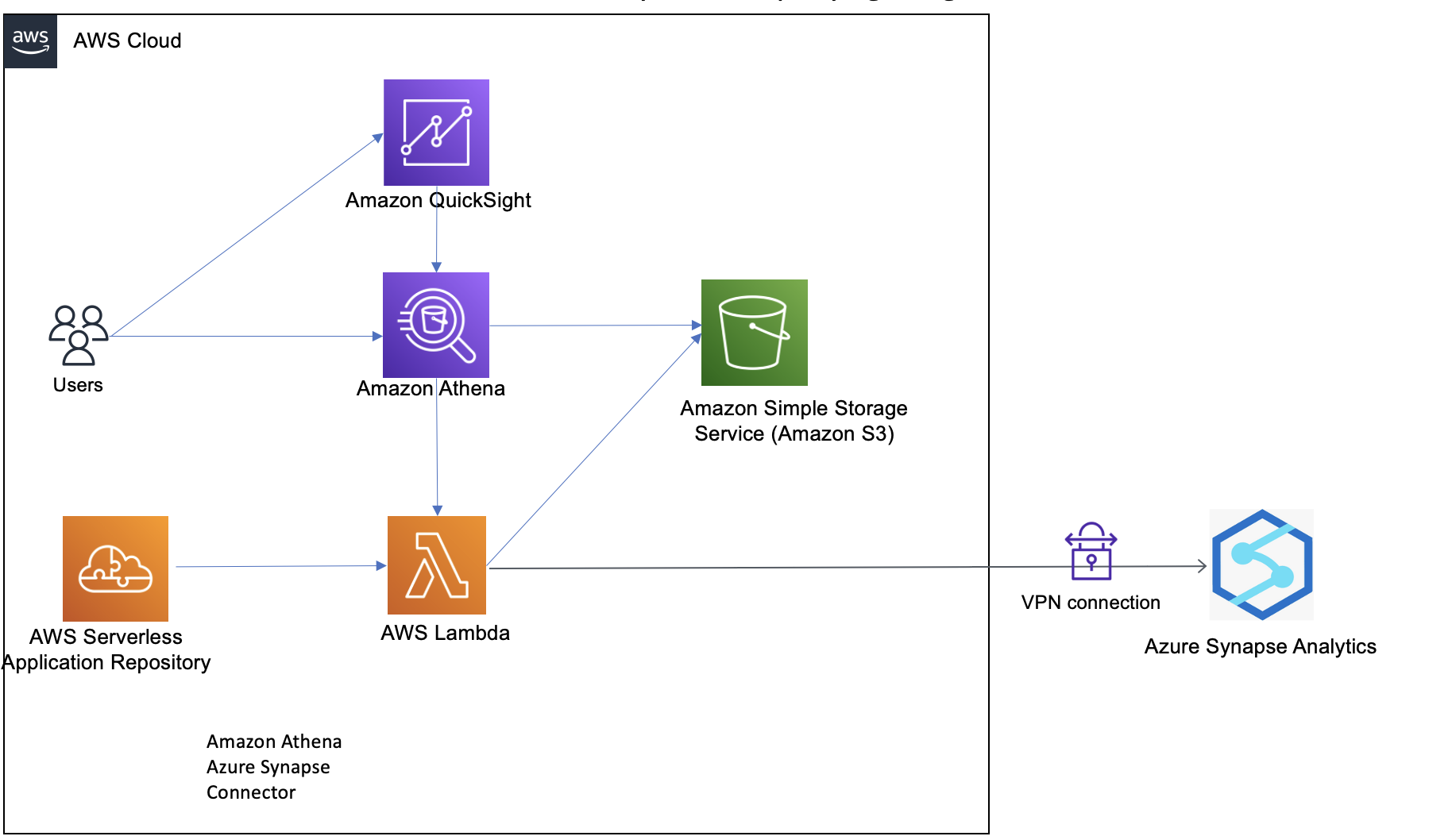
Athena uses data source connectors that run on AWS Lambda to run federated queries. A data source connector is a piece of code that can translate between your target data source and Athena. You can think of a connector as an extension of Athena’s query engine. In this post, we use the Athena connector for Azure Synapse analytics that enables Athena to run SQL queries on your Azure Synapse databases using JDBC.

Solution overview

Consider the following reference architecture for visualizing data from Azure Synapse Analytics.

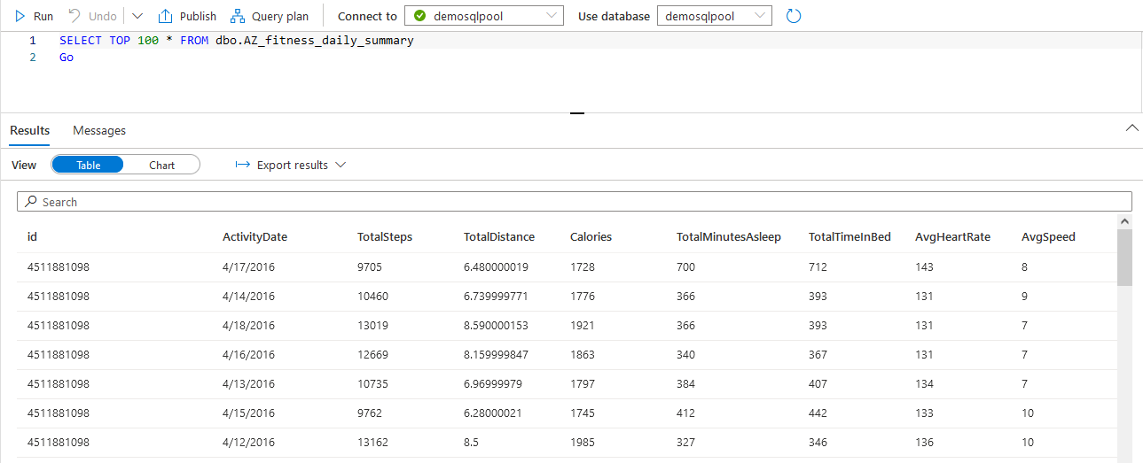
In order to explain this architecture, let’s walk through a sample use case of analyzing fitness data of users. Our sample dataset contains users’ fitness information like age, height, and weight, and daily run stats like miles, calories, average heart rate, and average speed, along with hours of sleep.

We run queries on this dataset to derive insights using visualizations in QuickSight. With QuickSight, you can create trends of daily miles run, keep track of the average heart rate over a period of time, and detect anomalies, if any. You can also track your daily sleep patterns and compare how rest impacts your daily activities. The out-of-the-box insights feature gives vital weekly insights that can help you be on top of your fitness goals. The following screenshot shows sample rows of our dataset stored in Azure Synapse.


Prerequisites

Make sure you have the following prerequisites:

  • An AWS account set up with QuickSight enabled. If you don’t have a QuickSight account, you can sign up for one. You can access the QuickSight free trial as part of the AWS Free Tier option.
  • An Azure account with data pre-loaded in Synapse. We use a sample fitness dataset in this post. We used a data generator to generate this data.
  • A virtual private connection (VPN) between AWS and Azure.

Note that the AWS resources for the steps in this post need to be in the same Region.

Configure a Lambda connector

To configure your Lambda connector, complete the following steps:

  1. Load the data.
    In the Azure account, the sample data for fitness devices is stored and accessed in an Azure Synapse Analytics workspace using a dedicated SQL pool table. The firewall settings for Synapse should allow for access to a VPC through a VPN. You can use your data or tables that you need to connect QuickSight to in this step.
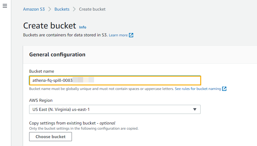
  2. On the Amazon S3 console, create a spillover bucket and note the name to use in a later step.
    This bucket is used for storing the spillover data for the Synapse connector.
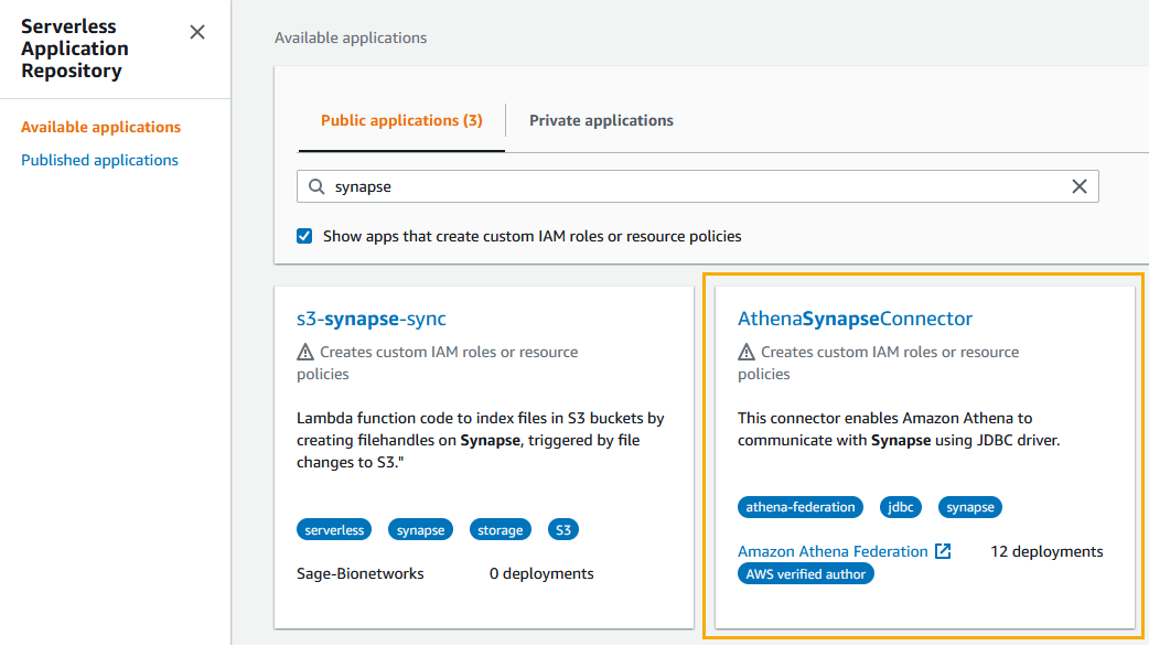
  3. On the AWS Serverless Application Repository console, choose Available applications in the navigation pane.
  4. On the Public applications tab, search for synapse and choose AthenaSynapseConnector with the AWS verified author tag.
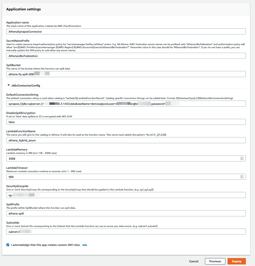
  5. Create the Lambda function with the following configuration:
    1. For Name, enter AthenaSynapseConnector.
    2. For SecretNamePrefix, enter AthenaJdbcFederation.
    3. For SpillBucket, enter the name of the S3 bucket you created.
    4. For DefaultConnectionString, enter the JDBC connection string from the Azure SQL pool connection strings property.
    5. For LambdaFunctionName, enter a function name.
    6. For SecurityGroupIds and SubnetIds, enter the security group and subnet for your VPC (this is needed for the template to run successfully).
    7. Leave the remaining values as their default.
  6. Choose Deploy.
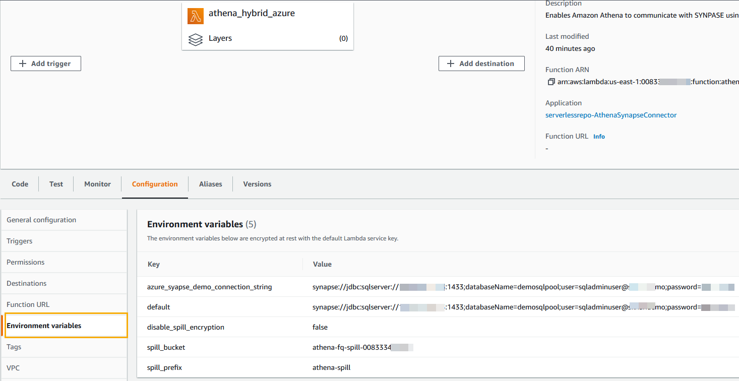
  7. After the function is deployed successfully, navigate to the athena_hybrid_azure function.
  8. On the Configurations tab, choose Environment variables in the navigation pane.
  9. Add the key azure_synapse_demo_connection_string with the same value as the default key (the JDBC connection string from the Azure SQL pool connection strings property).

    For this post, we removed the VPC configuration.
  10. Choose VPC in the navigation pane and choose None to remove the VPC configuration.
    Now you’re ready to configure the data source.
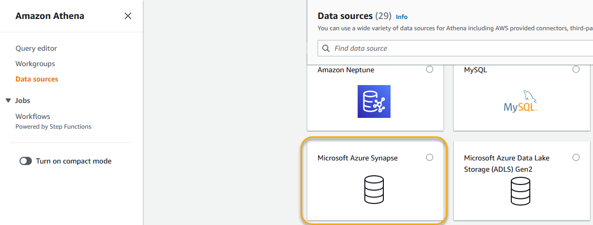
  11. On the Athena console, choose Data sources in the navigation pane.
  12. Choose Create data source.
  13. Choose Microsoft Azure Synapse as your data source.
  14. Choose Next.
  15. Create a data source with the following parameters:
    1. For Data source name, enter azure_synapse_demo.
    2. For Connection details, choose the Lambda function athena_hybrid_azure.
  16. Choose Next.

Create a dataset on QuickSight to read the data from Azure Synapse

Now that the configuration on the Athena side is complete, let’s configure QuickSight.

  1. On the QuickSight console, on the user name menu, choose Manage QuickSight.
  2. Choose Security & permissions in the navigation pane.
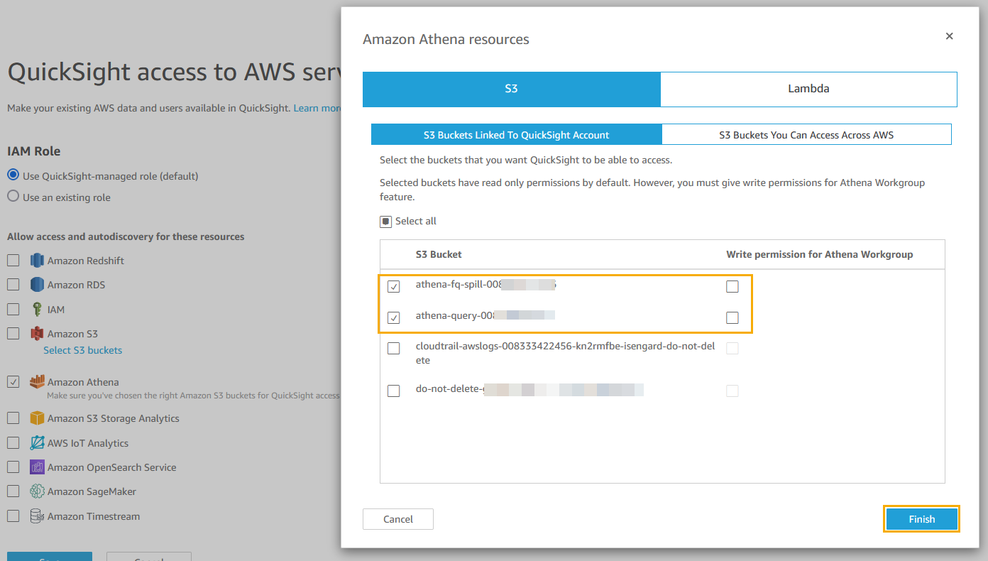
  3. Under QuickSight access to AWS services, choose Manage.
  4. Choose Amazon Athena and in the pop-up permissions box, choose Next.
  5. On the S3 Bucket tab, select the spill bucket you created earlier.
  6. On the Lambda tab, select the athena_hybrid_azure function.
  7. Choose Finish.
  8. If the QuickSight access to AWS services window appears, choose Save.
  9. Choose the QuickSight icon on the top left and choose New dataset.
  10. Choose Athena as the data source.
  11. For Data source name, enter a name.
  12. Check the Athena workgroup settings where the Athena data source was created.
  13. Choose Create data source.
  14. Choose the catalog azure_synapse_demo and the database dbo.
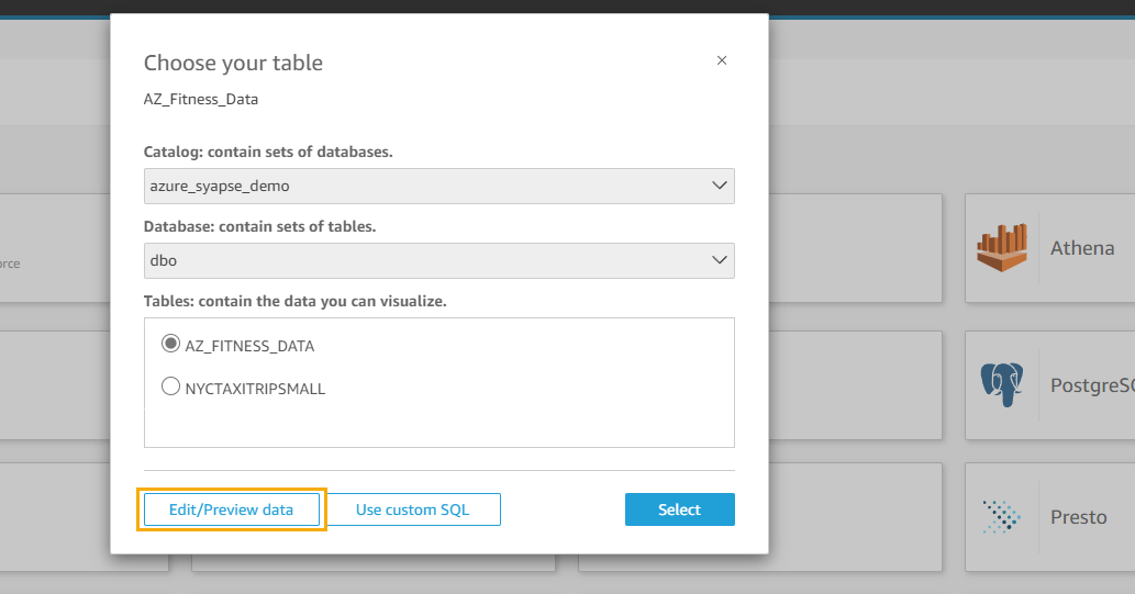
  15. Choose Edit/Preview data.
  16. Change the query mode to SPICE.
  17. Choose Publish & Visualize.
  18. Create an analysis in QuickSight.
  19. Publish a QuickSight dashboard.

If you’re new to QuickSight or looking to build stunning dashboards, this workshop provides step-by-step instructions to grow your dashboard building skills from basic to advanced level. The following screenshot is an example dashboard to give you some inspiration.

Clean up

To avoid ongoing charges, complete the following steps:

  1. Delete the S3 bucket created for the Athena spill data.
  2. Delete the Athena data source.
  3. On the AWS CloudFormation console, select the stack you created for AthenaSynapseConnector and choose Delete.
    This will delete the created resources, such as the Lambda function. Check the stack’s Events tab to track the progress of the deletion, and wait for the stack status to change to DELETE_COMPLETE.
  4. Delete the QuickSight datasets.
  5. Delete the QuickSight analysis.
  6. Delete your QuickSight subscription and close the account.

Conclusion

In this post, we showed you how to overcome the challenges of connecting to and analyzing data in other clouds by using AWS analytics services to connect to Azure Synapse Analytics with Athena Federated Query and QuickSight. We also showed you how to visualize and derive insights from the fitness data using QuickSight. With QuickSight and Athena Federated Query, organizations can now access additional data sources beyond those already supported natively by QuickSight. If you have data in sources other than Amazon S3, you can use Athena Federated Query to analyze the data in place or build pipelines that extract and store data in Amazon S3.

For more information and resources for QuickSight and Athena, visit Analytics on AWS.


About the authors

Harish Rajagopalan is a Senior Solutions Architect at Amazon Web Services. Harish works with enterprise customers and helps them with their cloud journey.

Salim Khan is a Specialist Solutions Architect for Amazon QuickSight. Salim has over 16 years of experience implementing enterprise business intelligence (BI) solutions. Prior to AWS, Salim worked as a BI consultant catering to industry verticals like Automotive, Healthcare, Entertainment, Consumer, Publishing and Financial Services. He has delivered business intelligence, data warehousing, data integration and master data management solutions across enterprises.

Sriram Vasantha is a Senior Solutions Architect at AWS in Central US helping customers innovate on the cloud. Sriram focuses on application and data modernization, DevSecOps, and digital transformation. In his spare time, Sriram enjoys playing different musical instruments like Piano, Organ, and Guitar.

Adarsha Nagappasetty is a Senior Solutions Architect at Amazon Web Services. Adarsha works with enterprise customers in Central US and helps them with their cloud journey. In his spare time, Adarsha enjoys spending time outdoors with his family!

Explore your data lake using Amazon Athena for Apache Spark

Post Syndicated from Pathik Shah original https://aws.amazon.com/blogs/big-data/explore-your-data-lake-using-amazon-athena-for-apache-spark/

Amazon Athena now enables data analysts and data engineers to enjoy the easy-to-use, interactive, serverless experience of Athena with Apache Spark in addition to SQL. You can now use the expressive power of Python and build interactive Apache Spark applications using a simplified notebook experience on the Athena console or through Athena APIs. For interactive Spark applications, you can spend less time waiting and be more productive because Athena instantly starts running applications in less than a second. And because Athena is serverless and fully managed, analysts can run their workloads without worrying about the underlying infrastructure.

Data lakes are a common mechanism to store and analyze data because they allow companies to manage multiple data types from a wide variety of sources, and store this data, structured and unstructured, in a centralized repository. Apache Spark is a popular open-source, distributed processing system optimized for fast analytics workloads against data of any size. It’s often used to explore data lakes to derive insights. For performing interactive data explorations on the data lake, you can now use the instant-on, interactive, and fully managed Apache Spark engine in Athena. It enables you to be more productive and get started quickly, spending almost no time setting up infrastructure and Spark configurations.

In this post, we show how you can use Athena for Apache Spark to explore and derive insights from your data lake hosted on Amazon Simple Storage Service (Amazon S3).

Solution overview

We showcase reading and exploring CSV and Parquet datasets to perform interactive analysis using Athena for Apache Spark and the expressive power of Python. We also perform visual analysis using the pre-installed Python libraries. For running this analysis, we use the built-in notebook editor in Athena.

For the purpose of this post, we use the NOAA Global Surface Summary of Day public dataset from the Registry of Open Data on AWS, which consists of daily weather summaries from various NOAA weather stations. The dataset is primarily in plain text CSV format. We have transformed the entire and subsets of the CSV dataset into Parquet format for our demo.

Before running the demo, we want to introduce the following concepts related to Athena for Spark:

  • Sessions – When you open a notebook in Athena, a new session is started for it automatically. Sessions keep track of the variables and state of notebooks.
  • Calculations – Running a cell in a notebook means running a calculation in the current session. As long as a session is running, calculations use and modify the state that is maintained for the notebook.

For more details, refer to Session and Calculations.

Prerequisites

For this demo, you need the following prerequisites:

  • An AWS account with access to the AWS Management Console
  • Athena permissions on the workgroup DemoAthenaSparkWorkgroup, which you create as part of this demo
  • AWS Identity and Access Management (IAM) permissions to create, read, and update the IAM role and policies created as part of the demo
  • Amazon S3 permissions to create an S3 bucket and read the bucket location

The following policy grants these permissions. Attach it to the IAM role or user you use to sign in to the console. Make sure to provide your AWS account ID and the Region in which you’re running the demo.

{
    "Version": "2012-10-17",
    "Statement": [
        {
            "Effect": "Allow",
            "Action": "athena:*",
            "Resource": "arn:aws:athena:<REGION>:<ACCOUNT_ID>:workgroup/DemoAthenaSparkWorkgroup"
        },
        {
            "Effect": "Allow",
            "Action": [
                "iam:CreatePolicy",
                "iam:GetRole",
                "iam:ListAttachedRolePolicies",
                "iam:CreateRole",
                "iam:AttachRolePolicy",
                "iam:PutRolePolicy",
                "iam:ListRolePolicies",
                "iam:GetRolePolicy",
                "iam:PassRole"
            ],
            "Resource": [
                "arn:aws:iam::<ACCOUNT_ID>:role/service-role/AWSAthenaSparkExecutionRole-*",
                "arn:aws:iam::<ACCOUNT_ID>:policy/service-role/AWSAthenaSparkRolePolicy-*"
            ]
        },
        {
            "Effect": "Allow",
            "Action": [
                "s3:CreateBucket",
                "s3:GetBucketLocation"
            ],
            "Resource": "arn:aws:s3:::<ACCOUNT_ID>-<REGION>-athena-results-bucket-*"
        },
        {
            "Effect": "Allow",
            "Action": [
                "iam:ListPolicies",
                "iam:ListRoles",
                "athena:ListWorkGroups",
                "athena:ListEngineVersions"
            ],
            "Resource": "*"
        }
    ]
}

Create your Athena workgroup

We create a new Athena workgroup with Spark as the engine. Complete the following steps:

  1. On the Athena console, choose Workgroups in the navigation pane.
  2. Choose Create workgroup.
  3. For Workgroup name, enter DemoAthenaSparkWorkgroup.
    Make sure to enter the exact name because the preceding IAM permissions are scoped down for the workgroup with this name.
  4. For Analytics engine, choose Apache Spark.
  5. For Additional configurations, select Use defaults.
    The defaults include the creation of an IAM role with the required permissions to run Spark calculations on Athena and an S3 bucket to store calculation results. It also sets the notebook (which we create later) encryption key management to an AWS Key Management Service (AWS KMS) key owned by Athena.
  6. Optionally, add tags to your workgroup.
  7. Choose Create workgroup.

Modify the IAM role

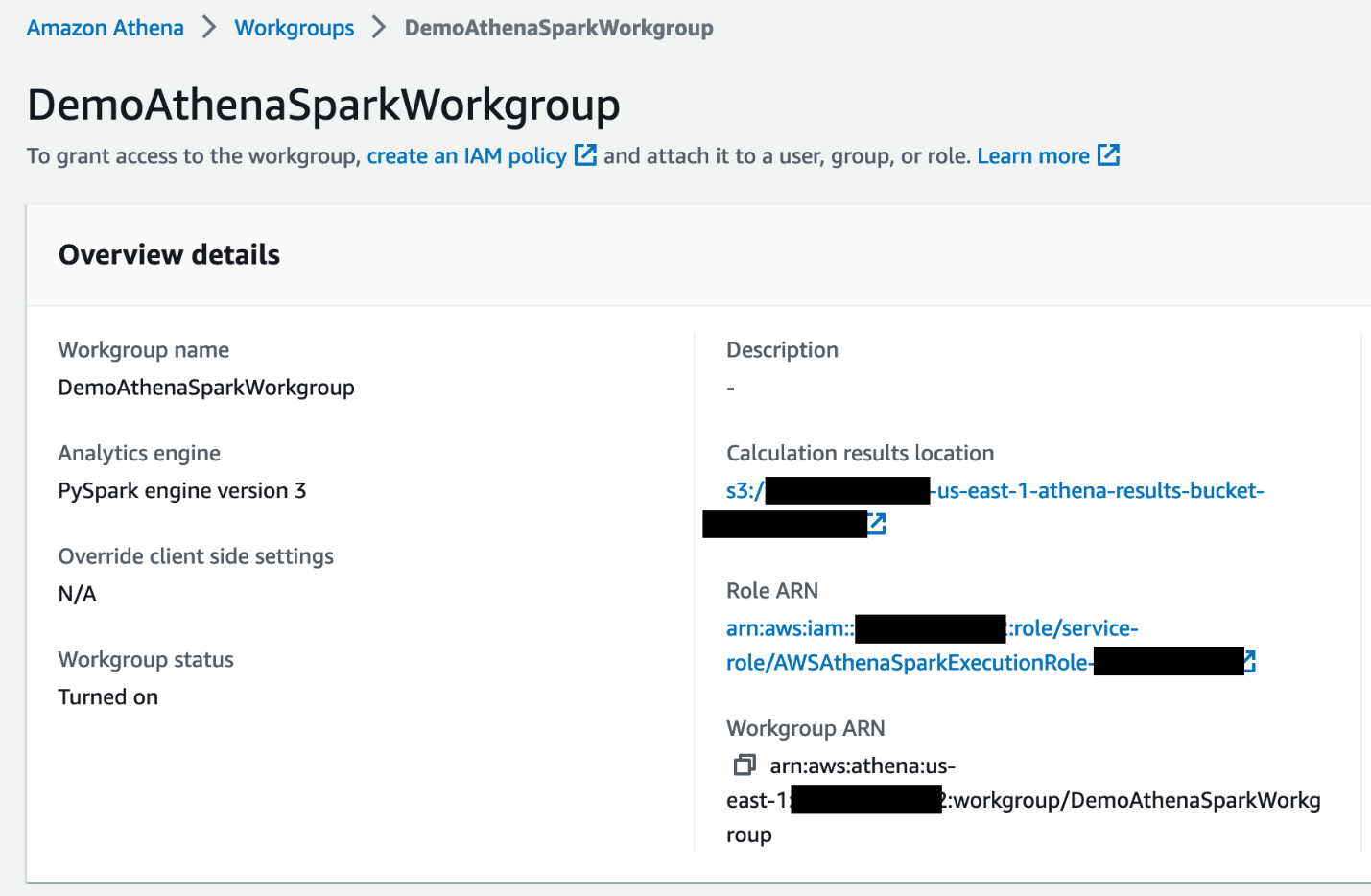
Creating the workgroup creates a new IAM role. Choose the newly created workgroup, then the value under Role ARN to be redirected to the IAM console.

Add the following permission as an inline policy to the IAM role created earlier. This allows the role to read the S3 datasets. For instructions, refer to the section To embed an inline policy for a user or role (console) in Adding IAM identity permissions (console).

{
    "Version": "2012-10-17",
    "Statement": [
        {
            "Sid": "VisualEditor0",
            "Effect": "Allow",
            "Action": [
                "s3:GetObject",
                "s3:ListBucket"
            ],
            "Resource": [
                "arn:aws:s3:::athena-examples-us-east-1/athenasparkblog/noaa-gsod-pds/parquet/*",
                "arn:aws:s3:::noaa-gsod-pds/2022/*",
                "arn:aws:s3:::noaa-gsod-pds",
                "arn:aws:s3:::athena-examples-us-east-1"
            ]
        }
    ]
}

Set up your notebook

To run the analysis on Spark on Athena, we need a notebook. Complete the following steps to create one:

  1. On the Athena console, choose Notebook Editor.
  2. Choose the newly created workgroup DemoAthenaSparkWorkgroup on the drop-down menu.
  3. Choose Create Notebook.
  4. Provide a notebook name, for example AthenaSparkBlog.
  5. Keep the default session parameters.
  6. Choose Create.

Your notebook should now be loaded, which means you can start running Spark code. You should see the following screenshot.

Explore the dataset

Now that we have workgroup and notebook created, let’s start exploring the NOAA Global Surface Summary of Day dataset. The datasets used in this post are stored in the following locations:

  • CSV data for year 2022 – s3://noaa-gsod-pds/2022/
  • Parquet data for year 2021 – s3://athena-examples-us-east-1/athenasparkblog/noaa-gsod-pds/parquet/2021/
  • Parquet data for year 2020 – s3://athena-examples-us-east-1/athenasparkblog/noaa-gsod-pds/parquet/2020/
  • Entire dataset in Parquet format (until October 2022) – s3://athena-examples-us-east-1/athenasparkblog/noaa-gsod-pds/parquet/historical/

In the rest of this post, we show PySpark code snippets. Copy the code and enter it in the notebook’s cell. Press Shift+Enter to run the code as a calculation. Alternatively, you can choose Run. Add more cells to run subsequent code snippets.

We start by reading the CSV dataset for the year 2022 and print its schema to understand the columns contained in the dataset. Run the following code in the notebook cell:

year_22_csv = spark.read.option("header","true").csv(f"s3://noaa-gsod-pds/2022/")
year_22_csv.printSchema()

We get the following output.

We were able to submit the preceding code as a calculation instantly using the notebook.

Let’s continue exploring the dataset. Looking at the columns in the schema, we’re interested in previewing the data for the following attributes in 2022:

  • TEMP – Mean temperature
  • WDSP – Mean wind speed
  • GUST – Maximum wind gust
  • MAX – Maximum temperature
  • MIN – Minimum temperature
  • Name – Station name

Run the following code:

year_22_csv.select('NAME','DATE','TEMP','WDSP','GUST','MAX','MIN').show()

We get the following output.

Now we have an idea of what the dataset looks like. Next, let’s perform some analysis to find the maximum recorded temperature for the Seattle-Tacoma Airport in 2022. Run the following code:

from pyspark.sql.functions import max

year_22_csv.filter("NAME == 'SEATTLE TACOMA AIRPORT, WA US'").agg(max("MAX").alias("max_temp_yr_2022")).show()

We get the following output.

Next, we want to find the maximum recorded temperature for each month of 2022. For this, we use the Spark SQL feature of Athena. First, we need to create a temporary view on the year_22_csv data frame. Run the following code:

year_22_csv.createOrReplaceTempView("y22view")

To run our Spark SQL query, we use %%sql magic:

%%sql
select month(to_date(date,'yyyy-MM-dd')) as month_yr_22,max(MAX) as max_temp 
from y22view where NAME == 'SEATTLE TACOMA AIRPORT, WA US' 
group by 1

We get the following output.

The output of the preceding query produces the month in numeric form. To make it more readable, let’s convert the month numbers into month names. For this, we use a user-defined function (UDF) and register it to use in the Spark SQL queries for the rest of the notebook session. Run the following code to create and register the UDF:

import calendar

# UDF to convert month number to month name
spark.udf.register("month_name_udf",lambda x: calendar.month_name[int(x)])

We rerun the query to find the maximum recorded temperature for each month of 2022 but with the month_name_udf UDF we just created. Also, this time we sort the results based on the maximum temperature value. See the following code:

%%sql
select month_name_udf(month(to_date(date,'yyyy-MM-dd'))) as month_yr_22,
max(MAX) as max_temp
from y22view where NAME == 'SEATTLE TACOMA AIRPORT, WA US' 
group by 1 order by 2 desc

The following output shows the month names.

Until now, we have run interactive explorations for the year 2022 of the NOAA Global Surface Summary of Day dataset. Let’s say we want to compare the temperature values with the previous 2 years. We compare the maximum temperature across 2020, 2021, and 2022. As a reminder, the dataset for 2022 is in CSV format and for 2020 and 2021, the datasets are in Parquet format.

To continue with the analysis, we read the 2020 and 2021 Parquet datasets into the data frame and create temporary views on the respective data frames. Run the following code:

#Read the dataset
year_20_pq = spark.read.parquet(f"s3://athena-examples-us-east-1/athenasparkblog/noaa-gsod-pds/parquet/2020/")
year_21_pq = spark.read.parquet(f"s3://athena-examples-us-east-1/athenasparkblog/noaa-gsod-pds/parquet/2021/")

#Create temporary views
year_20_pq.createOrReplaceTempView("y20view")
year_21_pq.createOrReplaceTempView("y21view")

#Preview the datasets
print('Preview for year 2020:')
year_20_pq.select('NAME','DATE','TEMP','WDSP','GUST','MAX','MIN').show(1)
print('Preview for year 2021:')
year_21_pq.select('NAME','DATE','TEMP','WDSP','GUST','MAX','MIN').show(1)

We get the following output.

To compare the recorded maximum temperature for each month in 2020, 2021, and 2022, we perform a join operation on the three views created so far from their respective data frames. Also, we reuse the month_name_udf UDF to convert month number to month name. Run the following code:

%%sql
select month_name_udf(month(to_date(y21.DATE,'yyyy-MM-dd'))) as month, max(y20.max) as max_temp_2020, 
max(y21.max) as max_temp_2021, max(y22.max) as max_temp_2022 \
from y20view y20 inner join y21view y21 inner join y22view y22 \
on month(to_date(y20.DATE,'yyyy-MM-dd')) = month(to_date(y21.DATE,'yyyy-MM-dd'))
and month(to_date(y21.DATE,'yyyy-MM-dd')) = month(to_date(y22.DATE,'yyyy-MM-dd')) \
where y20.NAME == 'SEATTLE TACOMA AIRPORT, WA US' and y21.NAME == 'SEATTLE TACOMA AIRPORT, WA US' and y22.NAME == 'SEATTLE TACOMA AIRPORT, WA US' \
group by 1

We get the following output.

So far, we’ve read CSV and Parquet datasets, run analysis on the individual datasets, and performed join and aggregation operations on them to derive insights instantly in an interactive mode. Next, we show how you can use the pre-installed libraries like Seaborn, Matplotlib, and Pandas for Spark on Athena to generate a visual analysis. For the full list of preinstalled Python libraries, refer to List of preinstalled Python libraries.

We plot a visual analysis to compare the recorded maximum temperature values for each month in 2020, 2021, and 2022. Run the following code, which creates a Spark data frame from the SQL query, converts it into a Pandas data frame, and uses Seaborn and Matplotlib for plotting:

import seaborn as sns
import matplotlib.pyplot as plt

y20_21_22=spark.sql("select month(to_date(y21.DATE,'yyyy-MM-dd')) as month, max(y20.max) as max_temp_yr_2020, \
max(y21.max) as max_temp_yr_2021, max(y22.max) as max_temp_yr_2022 \
from y20view y20 inner join y21view y21 inner join y22view y22 \
on month(to_date(y20.DATE,'yyyy-MM-dd')) = month(to_date(y21.DATE,'yyyy-MM-dd')) \
and month(to_date(y21.DATE,'yyyy-MM-dd')) = month(to_date(y22.DATE,'yyyy-MM-dd')) \
where y20.NAME == 'SEATTLE TACOMA AIRPORT, WA US' and y21.NAME == 'SEATTLE TACOMA AIRPORT, WA US' and y22.NAME == 'SEATTLE TACOMA AIRPORT, WA US' \
group by 1 order by 1")

#convert to pandas dataframe
y20_21_22=y20_21_22.toPandas()

#change datatypes to float for plotting
y20_21_22['max_temp_yr_2020']= y20_21_22['max_temp_yr_2020'].astype(float)
y20_21_22['max_temp_yr_2021']= y20_21_22['max_temp_yr_2021'].astype(float)
y20_21_22['max_temp_yr_2022']= y20_21_22['max_temp_yr_2022'].astype(float)

# Unpivot dataframe from wide to long format for plotting
y20_21_22=y20_21_22.melt('month',var_name='max_temperature', \
             value_name='temperature')

plt.clf()

sns.catplot(data=y20_21_22,x='month',y='temperature', hue='max_temperature', \
            sort=False, kind='point', height=4, aspect=1.5)
%matplot plt

The following graph shows our output.

Next, we plot a heatmap showing the maximum temperature trend for each month across all the years in the dataset. For this, we have converted the entire CSV dataset (until October 2022) into Parquet format and stored it in s3://athena-examples-us-east-1/athenasparkblog/noaa-gsod-pds/parquet/historical/.

Run the following code to plot the heatmap:

noaa = spark.read.parquet(f"s3://athena-examples-us-east-1/athenasparkblog/noaa-gsod-pds/parquet/historical/")
noaa.createOrReplaceTempView("noaaview")

#query to find maximum temperature for each month from year 1973 to 2022
year_hist=spark.sql("select month(to_date(date,'yyyy-MM-dd')) as month, \
year(to_date(date,'yyyy-MM-dd')) as year,  cast(max(temp) as float) as temp \
from noaaview where NAME == 'SEATTLE TACOMA AIRPORT, WA US' group by 1,2") 

# convert spark dataframe to pandas
year_hist=year_hist.toPandas()
year_hist=year_hist.pivot("month","year","temp")

plt.clf()
grid_kws = {"height_ratios": (0.9, .05), "hspace": .5}
f, (ax, cbar_ax) = plt.subplots(2, gridspec_kw=grid_kws)

sns.heatmap(year_hist, ax=ax, cbar_ax=cbar_ax, cmap="RdYlBu_r", \
            cbar_kws={"orientation": "horizontal"})
%matplot plt

We get the following output.

From the potting, we can see the trend has been almost similar across the years, where the temperature rises during summer months and lowers as winter approaches in the Seattle-Tacoma Airport area. You can continue exploring the datasets further, running more analyses and plotting more visuals to get the feel of the interactive and instant-on experience Athena for Apache Spark offers.

Clean up resources

When you’re done with the demo, make sure to delete the S3 bucket you created to store the workgroup calculations to avoid storage costs. Also, you can delete the workgroup, which deletes the notebook as well.

Conclusion

In this post, we saw how you can use the interactive and serverless experience of Athena for Spark as the engine to run calculations instantly. You just need to create a workgroup and notebook to start running the Spark code. We explored datasets stored in different formats in an S3 data lake and ran interactive analyses to derive various insights. Also, we ran visual analyses by plotting charts using the preinstalled libraries. To learn more about Spark on Athena, refer to Using Apache Spark in Amazon Athena.


About the Authors

Pathik Shah is a Sr. Big Data Architect on Amazon Athena. He joined AWS in 2015 and has been focusing in the big data analytics space since then, helping customers build scalable and robust solutions using AWS analytics services.

Raj Devnath is a Sr. Product Manager at AWS working on Amazon Athena. He is passionate about building products customers love and helping customers extract value from their data. His background is in delivering solutions for multiple end markets, such as finance, retail, smart buildings, home automation, and data communication systems.

How to use Amazon Macie to preview sensitive data in S3 buckets

Post Syndicated from Koulick Ghosh original https://aws.amazon.com/blogs/security/how-to-use-amazon-macie-to-preview-sensitive-data-in-s3-buckets/

Security teams use Amazon Macie to discover and protect sensitive data, such as names, payment card data, and AWS credentials, in Amazon Simple Storage Service (Amazon S3). When Macie discovers sensitive data, these teams will want to see examples of the actual sensitive data found. Reviewing a sampling of the discovered data helps them quickly confirm that the object is truly sensitive according to their data protection and privacy policies.

In this post, we walk you through how your data security teams are able to use a new capability in Amazon Macie to retrieve up to 10 examples of sensitive data found in your S3 objects, so that you are able to confirm the nature of the data at a glance. Additionally, we will discuss how you are able to control who is able to use this capability, so that only authorized personnel have permissions to view these examples.

The challenge customers face

After a Macie sensitive data discovery job is run, security teams start their work. The security team will review the Macie findings to investigate the discovered sensitive data and decide what actions to take to protect such data. The findings provide details that include the severity of the finding, information on the affected S3 object, and a summary of the type, location, and amount of sensitive data found. However, Macie findings only contain pointers to data that Macie found in the object. In order to complete their investigation, customers in the past had to do additional work to extract the contents of a sensitive object, such as navigating to a different AWS account where the object is located, downloading and manually searching for keywords in a file editor, or writing and refining SQL queries by using Amazon S3 Select. The investigations are further slowed down when the object type is one that is not easily readable without additional tooling, such as big-data file types like Avro and Parquet. By using the Macie capability to retrieve sensitive data samples, you are able to review the discovered data and make decisions concerning the finding remediation.

Prerequisites

To implement the ability to retrieve and reveal samples of sensitive data, you’ll need the following prerequisites:

  • Enable Amazon Macie in your AWS account. For instructions, see Getting started with Amazon Macie.
  • Set your account as the delegated Macie administrator account and enable Macie in at least one member account by using AWS Organizations. In this post, we will refer to the delegated administrator account as Account A and the member account as Account B.
  • Configure Macie detailed classification results in Account A.

    Note: The detailed classification results contain a record for each Amazon S3 object that you configure the job to analyze, and include the location of up to 1,000 occurrences of each type of sensitive data that Macie found in an object. Macie uses the location information in the detailed classification results to retrieve the examples of sensitive data. The detailed classification results are stored in an S3 bucket of your choice. In this post, we will refer to this bucket as DOC-EXAMPLE-BUCKET1.

  • Create an S3 bucket that contains sensitive data in Account B. In this post, we will refer to this bucket as DOC-EXAMPLE-BUCKET2.

    Note: You should enable server-side encryption on this bucket by using customer managed AWS Key Management Service (AWS KMS) keys (a type of encryption known as SSE-KMS).

  • (Optional) Add sensitive data to DOC-EXAMPLE-BUCKET2. This post uses a sample dataset that contains fake sensitive data. You are able to download this sample dataset, unarchive the .zip folder, and follow these steps to upload the objects to S3. This is a synthetic dataset generated by AWS that we will use for the examples in this post. All data in this blog post has been artificially created by AWS for demonstration purposes and has not been collected from any individual person. Similarly, such data does not relate back to any individual person, nor is it intended to.
  • Create and run a sensitive data discovery job from Account A to analyze the contents of DOC-EXAMPLE-BUCKET2.
  • (Optional) Set up the AWS Command Line Interface (AWS CLI).

Configure Macie to retrieve and reveal examples of sensitive data

In this section, we’ll describe how to configure Macie so that you are able to retrieve and view examples of sensitive data from Macie findings.

To configure Macie (console)

  • In the AWS Management Console, in the Macie delegated administrator account (Account A), follow these steps from the Amazon Macie User Guide.

To configure Macie (AWS CLI)

  1. Confirm that you have Macie enabled.
    	$ aws macie2 get-macie-session --query 'status'
    	// The expected response is "ENABLED"

  2. Confirm that you have configured the detailed classification results bucket.
    	$ aws macie2 get-classification-export-configuration
    
    	// The expected response is:
    	{
       	 "configuration": {
       		 	    "s3Destination": {
            		    "bucketName": " DOC-EXAMPLE-BUCKET1 ",
               			"kmsKeyArn": "arn:aws:kms:<YOUR-REGION>:<YOUR-ACCOUNT-ID>:key/<KEY-USED-TO-ENCRYPT-DOC-EXAMPLE-BUCKET1>"
         		  	 }
    		}	
    	} 

  3. Create a new KMS key to encrypt the retrieved examples of sensitive data. Make sure that the key is created in the same AWS Region where you are operating Macie.
    $ aws kms create-key
    {
        "KeyMetadata": {
            "Origin": "AWS_KMS",
            "KeyId": "<YOUR-KEY-ID>",
            "Description": "",
            "KeyManager": "CUSTOMER",
            "Enabled": true,
            "KeySpec": "SYMMETRIC_DEFAULT",
            "CustomerMasterKeySpec": "SYMMETRIC_DEFAULT",
            "KeyUsage": "ENCRYPT_DECRYPT",
            "KeyState": "Enabled",
            "CreationDate": 1502910355.475,
            "Arn": "arn:aws:kms: <YOUR-AWS-REGION>:<AWS-ACCOUNT-A>:key/<YOUR-KEY-ID>",
            "AWSAccountId": "<AWS-ACCOUNT-A>",
            "MultiRegion": false
            "EncryptionAlgorithms": [
                "SYMMETRIC_DEFAULT"
            ],
        }
    }

  4. Give this key the alias REVEAL-KMS-KEY.
    $ aws kms CreateAlias
    {
       "AliasName": " <REVEAL-KMS-KEY> ",
       "TargetKeyId": "<YOUR-KEY-ID>"
    }

  5. Enable the feature in Macie and configure it to encrypt the data by using REVEAL-KMS-KEY. You do not specify a key policy for your new KMS key in this step. The key policy will be discussed later in the post.
    $ aws macie2 update-reveal-configuration --configuration '{"status":"ENABLED","kmsKeyId":"alias/ <REVEAL-KMS-KEY> "}'
    
    // The expected response is:
    {
        "configuration": {
            "kmsKeyId": "arn:aws:kms:<YOUR-REGION>: <YOUR ACCOUNT ID>:key/<REVEAL-KMS-KEY>.",
            "status": "ENABLED"
        }
    }

Control access to read sensitive data and protect data displayed in Macie

This new Macie capability uses the AWS Identity and Access Management (IAM) policies, S3 bucket policies, and AWS KMS key policies that you have defined in your accounts. This means that in order to see examples through the Macie console or by invoking the Macie API, the IAM principal needs to have read access to the S3 object and to decrypt the object if it is server-side encrypted. It’s important to note that Macie uses the IAM permissions of the AWS principal to locate, retrieve, and reveal the samples and does not use the Macie service-linked role to perform these tasks.

Using the setup discussed in the previous section, you will walk through how to control access to the ability to retrieve and reveal sensitive data examples. To recap, you created and ran a discovery job from the Amazon Macie delegated administrator account (Account A) to analyze the contents of DOC-EXAMPLE-BUCKET2 in a member account (Account B). You configured Macie to retrieve examples and to encrypt the examples of sensitive data with the REVEAL-KMS-KEY.

The next step is to create and use an IAM role that will be assumed by other users in Account A to retrieve and reveal examples of sensitive data discovered by Macie. In this post, we’ll refer to this role as MACIE-REVEAL-ROLE.

To apply the principle of least privilege and allow only authorized personnel to view the sensitive data samples, grant the following permissions so that Macie users who assume MACIE-REVEAL-ROLE will be able to successfully retrieve and reveal examples of sensitive data:

  • Step 1 – Update the IAM policy for MACIE-REVEAL-ROLE.
  • Step 2 – Update the KMS key policy for REVEAL-KMS-KEY.
  • Step 3 – Update the S3 bucket policy for DOC-EXAMPLE-BUCKET2 and the KMS key policy used for its server-side encryption in Account B.

After you grant these permissions, MACIE-REVEAL-ROLE is succcesfully able to retrieve and reveal examples of sensitive data in DOC-EXAMPLE-BUCKET2, as shown in Figure 1.

Figure 1: Macie runs the discovery job from the delegated administrator account in a member account, and MACIE-REVEAL-ROLE retrieves examples of sensitive data

Figure 1: Macie runs the discovery job from the delegated administrator account in a member account, and MACIE-REVEAL-ROLE retrieves examples of sensitive data

Step 1: Update the IAM policy

Provide the following required permissions to MACIE-REVEAL-ROLE:

  1. Allow GetObject from DOC-EXAMPLE-BUCKET2 in Account B.
  2. Allow decryption of DOC-EXAMPLE-BUCKET2 if it is server-side encrypted with a customer managed key (SSE-KMS).
  3. Allow GetObject from DOC-EXAMPLE-BUCKET1.
  4. Allow decryption of the Macie discovery results.
  5. Allow the necessary Macie actions to retrieve and reveal sensitive data examples.

To set up the required permissions

  • Use the following commands to provide the permissions. Make sure to replace the placeholders with your own data.
    {
        "Version": "2012-10-17",
        "Statement": [
    	{
                "Sid": "AllowGetFromCompanyDataBucket",
                "Effect": "Allow",
                "Action": "s3:GetObject",
                "Resource": "arn:aws:s3:::<DOC-EXAMPLE-BUCKET2>/*"
            },
            {
                "Sid": "AllowKMSDecryptForCompanyDataBucket",
                "Effect": "Allow",
                "Action": [
                    "kms:Decrypt"
                ],
                "Resource": "arn:aws:kms:<AWS-Region>:<AWS-Account-B>:key/<KEY-USED-TO-ENCRYPT-DOC-EXAMPLE-BUCKET2>"
            },
            {
                "Sid": "AllowGetObjectfromMacieResultsBucket",
                "Effect": "Allow",
                "Action": "s3:GetObject",
                "Resource": "arn:aws:s3:::<DOC-EXAMPLE-BUCKET1>/*"
            },
    	{
                "Sid": "AllowKMSDecryptForMacieRoleDiscoveryBucket",
                "Effect": "Allow",
                "Action": [
                    "kms:Decrypt"
                ],
                "Resource": "arn:aws:kms:<AWS-REGION>:<AWS-ACCOUNT-A>:key/<KEY-USED-TO-ENCRYPT-DOC-EXAMPLE-BUCKET1>"
            },
    	{
                "Sid": "AllowActionsRetrieveAndReveal",
                "Effect": "Allow",
                "Action": [
                    "macie2:GetMacieSession",
                    "macie2:GetFindings",
                    "macie2:GetSensitiveDataOccurrencesAvailability",
                    "macie2:GetSensitiveDataOccurrences",
                    "macie2:ListFindingsFilters",
                    "macie2:GetBucketStatistics",
                    "macie2:ListMembers",
                    "macie2:ListFindings",
                    "macie2:GetFindingStatistics",
                    "macie2:GetAdministratorAccount",
                    "macie2:GetClassificationExportConfiguration",
                    "macie2:GetRevealConfiguration",
                    "macie2:DescribeBuckets"
                ],
                "Resource": "*” 
            }
        ]
    }

Step 2: Update the KMS key policy

Next, update the KMS key policy that is used to encrypt sensitive data samples that you retrieve and reveal in your delegated administrator account.

To update the key policy

  • Allow the MACIE-REVEAL-ROLE access to the KMS key that you created for protecting the retrieved sensitive data, using the following commands. Make sure to replace the placeholders with your own data.
    	{
                "Sid": "AllowMacieRoleDecrypt",
                "Effect": "Allow",
                "Principal": {
                    "AWS": "arn:aws:iam:<AWS-REGION>:<AWS-ACCOUNT-A>:role/<MACIE-REVEAL-ROLE>"
                },
                "Action": [
                    "kms:Decrypt",
                    "kms:DescribeKey",
                    "kms:GenerateDataKey"
                ],
                "Resource": "arn:aws:kms:<AWS-REGION>:<AWS-ACCOUNT-A>:key/<REVEAL-KMS-KEY>"
            }

Step 3: Update the bucket policy of the S3 bucket

Finally, update the bucket policy of the S3 bucket in member accounts, and update the key policy of the key used for SSE-KMS.

To update the S3 bucket policy and KMS key policy

  1. Use the following commands to update key policy for the KMS key used for server-side encryption of the DOC-EXAMPLE-BUCKET2 bucket in Account B.
    	{
                "Sid": "AllowMacieRoleDecrypt”
                "Effect": "Allow",
                "Principal": {
                    "AWS": "arn:aws:iam:<AWS-REGION>:<AWS-ACCOUNT-A>:role/<MACIE-REVEAL-ROLE>"
                },
                "Action": "kms:Decrypt",
                "Resource": "arn:aws:kms:<AWS-REGION>:<AWS-ACCOUNT-B>:key/<KEY-USED-TO-ENCRYPT-DOC-EXAMPLE-BUCKET2>"
      }

  2. Use the following commands to update the bucket policy of DOC-EXAMPLE-BUCKET2 to allow cross-account access for MACIE-REVEAL-ROLE to get objects from this bucket.
    {
        "Version": "2012-10-17",
        "Statement": [
            {
                "Sid": "AllowMacieRoleGet",
                "Effect": "Allow",
                "Principal": {
                    "AWS": "arn:aws:iam::<AWS-ACCOUNT-A>:role/<MACIE-REVEAL-ROLE>"
                },
                "Action": "s3:GetObject",
                "Resource": "arn:aws:s3:::<DOC-EXAMPLE-BUCKET2>/*"
            }
        ]
    }

Retrieve and reveal sensitive data samples

Now that you’ve put in place the necessary permissions, users who assume MACIE-REVEAL-ROLE will be able to conveniently retrieve and reveal sensitive data samples.

To retrieve and reveal sensitive data samples

  1. In the Macie console, in the left navigation pane, choose Findings, and select a specific finding. Under Sensitive Data, choose Review.
    Figure 2: The finding details panel

    Figure 2: The finding details panel

  2. On the Reveal sensitive data page, choose Reveal samples.
    Figure 3: The Reveal sensitive data page

    Figure 3: The Reveal sensitive data page

  3. Under Sensitive data, you will be able to view up to 10 examples of the sensitive data found by Amazon Macie.
    Figure 4: Examples of sensitive data revealed in the Amazon Macie console

    Figure 4: Examples of sensitive data revealed in the Amazon Macie console

You are able to find additional information on setting up the Macie Reveal function in the Amazon Macie User Guide.

Conclusion

In this post, we showed how you are to retrieve and review examples of sensitive data that were found in Amazon S3 using Amazon Macie. This capability will make it easier for your data protection teams to review the sensitive contents found in S3 buckets across the accounts in your AWS environment. With this information, security teams are able to quickly take remediation actions, such as updating the configuration of sensitive buckets, quarantining files with sensitive information, or sending a notification to the owner of the account where the sensitive data resides. In certain cases, you are able to add the examples to an allow list in Macie if you don’t want Macie to report those as sensitive data (for example, corporate addresses or sample data that is used for testing).

The following are links to additional resources that you will be able to use to expand your knowledge of Amazon Macie capabilities and features:

If you have feedback about this post, submit comments in the Comments section below. If you have questions about this post, start a new thread on Amazon Macie re:Post.

Want more AWS Security news? Follow us on Twitter.

Koulick Ghosh

Koulick Ghosh

Koulick is a Senior Product Manager in AWS Security based in Seattle, WA. He loves speaking with customers on how AWS Security services can help make them more secure. In his free-time, he enjoys playing the guitar, reading, and exploring the Pacific Northwest.

Author

Michael Ingoldby

Michael is a Senior Security Solutions Architect at AWS based in Frisco, Texas. He provides guidance and helps customers to implement AWS native security services. Michael has been working in the security domain since 2006. When he is not working, he enjoys spending time outdoors.

Robert Wu

Robert Wu

Robert is the Software Development Engineer for AWS Macie, working on enabling customers with more sensitive data discovery capabilities. In his free time, he enjoys exploring and contributing to various open-source projects to widen his domain knowledge.

Journey to adopt Cloud-Native DevOps platform Series #1: OfferUp modernized DevOps platform with Amazon EKS and Flagger to accelerate time to market

Post Syndicated from Purna Sanyal original https://aws.amazon.com/blogs/devops/journey-to-adopt-cloud-native-devops-platform-series-1-offerup-modernized-devops-platform-with-amazon-eks-and-flagger-to-accelerate-time-to-market/

In this two part series, we discuss the challenges faced by OfferUp, a Digital Native customer, to meet business growth and time-to-market. Their journey involved modernizing their existing DevOps platform, from the traditional monolith virtual machine (VM) based architecture to modern containerized architecture and running cloud-native applications for secured progressive delivery to accelerate time to market. This series will provide strategies, architecture patterns, and technical steps you can adopt to become more agile and innovative like OfferUp has.

OfferUp engineers were using the homegrown DevOps platform to build and release new services on the marketplace platform. In this first post, we discuss the key challenges encountered by OfferUp engineers with the existing DevOps platform, as well as how OfferUp modernized its DevOps platform with Amazon Elastic Kubernetes Service (Amazon EKS) and Flagger, automating production releases with progressive delivery techniques for faster time-to-market with new products and services. Amazon EKS is a managed container service to run and scale Kubernetes applications in the cloud or on-premises.

Previous DevOps architecture

OfferUp is a leading online and mobile customer to customer (C2C) marketplace where users can both buy and sell goods on the platform. Users can browse and purchase products from a broad range of categories, including furniture, clothing, sports equipment, toys, and many more. As a mobile-first company, OfferUp puts a great deal of emphasis on in-person communication between buyers and sellers.

OfferUp built a home grown, self-managed DevOps platform. This platform used a set of manual processes and third-party applications that allows both developers and operations engineers to build and deploy code to a production environment. The DevOps pipeline included topic areas such as source code control, continuous integration/continuous delivery (CI/CD), microservices, as well as development and test Methodologies. The following diagram depicts the previous architecture of OfferUp’s DevOps platform, which was self-managed on Amazon Elastic Compute Cloud (Amazon EC2).

Figure 1: Previous DevOps architecture of OfferUp

OfferUp used GitHub for code repositories. Once the source code was committed in the code repository, Jenkins pulled the source code from code repositories on a scheduled or on-demand basis and built Amazon Machine Images (AMI). The built image was deployed in production by a  custom built deployment tool, Vanaheim, which supports one-box canary deployment and full roll-out deployment strategies. The DevOps engineers used to manually create a deployment job in the Vanaheim portal and then manually monitor the test success rate and service metrics to detect any impact from the deployment. Once the success rate was reached, a full production roll out was performed from the Vanaheim portal.

Key challenges with previous DevOps pipeline

In 2020, OfferUp experienced significant transaction volume growth on its Marketplace platform with the increase of its user base. With OfferUp’s acquisition of LetGo in 2020, there was a need to build a scalable DevOps platform to support future integration and organic growth. The previous DevOps platform, designed and deployed over seven years ago, had reached the limits of its scalability, and could no longer keep up with the platform’s growth. The previous architecture was expensive to run and had a complex infrastructure that made it difficult to upgrade and add new features.

The following key factors drove the push for modernization:

  • Manual verification was required to check if the code was correctly deployed in one of the servers in production, and if the deployment was right in one server, then it was rolled out to other production servers. Full Rollout to production wasn’t automated due to frequent failures requiring manual rollbacks.
  • The previous platform required a longer deployment time (1–2 hours) due to the authoritative batch process, which sometimes caused delays in releasing and testing of new features.
  • The self-managed nature of the Jenkins and Vanaheim clusters was consuming far too much engineering time. Most of the institutional knowledge of this legacy platform was lost over the years and it didn’t align with OfferUp’s philosophy of small DevOps engineering teams. Innovation had stalled partly due to the difficulty of simultaneously upgrading the DevOps platform and releasing new features.

DevOps platform automation with Flagger and Gloo Ingress Controller on Amazon EKS

A key requirement for the next-generation system was that the new architecture would reduce the operational burden on engineering teams, deployment lifecycle, and total cost of ownership. OfferUp evaluated multiple managed container orchestration platforms for its DevOps Platform. It finally selected Amazon EKS for high availability, reducing the average time to deploy a change to the stack from hours to just a few minutes and reducing the complexity in managing and upgrading the Kubernetes cluster. On the Amazon EKS platform, OfferUp uses Flagger, a progressive delivery tool that automates the release process for applications running on Kubernetes. Flagger implements several deployment strategies (Canary releases, A/B testing, and Blue/Green mirroring) using the Gloo Edge ingress controller for traffic routing. Datadog is used as an observability service for monitoring the health of the deployments and effectively managing the canary to progressive delivery. For release analysis, Flagger runs a query on Datadog logs and uses Slack for alerting and notifications. The cloud native technology components of the architecture are described as follows:

Kubernetes and Amazon EKS – Kubernetes is an open-source system for automating the deployment, scaling, and management of containerized applications. Kubernetes is a graduate project in the CNCF. Amazon EKS is a fully-managed, certified Kubernetes conformant service that simplifies the process of building, securing, operating, and maintaining Kubernetes clusters on AWS. Amazon EKS integrates with core AWS services, such as Amazon CloudWatch, Auto Scaling Groups, and AWS Identity and Access Management (IAM) to provide a seamless experience for monitoring, scaling, and load balancing your containerized applications.

Helm – Helm manage Kubernetes applications. Helm Charts define, install, and upgrade even the most complex Kubernetes application. Charts are easy to create, version, share, and publish. If Kubernetes were an operating system, then Helm would be the package manager. Helm is a graduate project in the CNCF and is maintained by the Helm community.

Flagger – Flagger is a progressive delivery tool that automates the release process for applications running on Kubernetes. Flagger implements a control loop that gradually shifts traffic to the canary while measuring key performance indicators such as HTTP requests success rate, requests average duration, and pods health. Based on the set thresholds, a canary is either promoted or aborted and its analysis is pushed to a Slack channel. Flagger became a CNCF project – part of the Flux family of GitOps tools.

Gloo Edge – Gloo Edge is a feature-rich, Kubernetes-native ingress controller. Gloo Edge is exceptional in its function-level routing; its support for legacy apps, microservices, and serverless; its discovery capabilities; and its tight integration with leading open-source projects. Gloo Edge is uniquely designed to support hybrid applications, in which multiple technologies, architectures, protocols, and clouds can coexist.

Observability platform – Datadog’s integrations with Kubernetes, Docker, and AWS will let you track the full range of Amazon EKS metrics, as well as logs and performance data from your cluster and applications. Datadog gives you comprehensive coverage of your dynamic infrastructure and applications with features like auto discovery to track services across containers, sophisticated graphing, and alerting options.

Modernized DevOps architecture

In the new architecture, OfferUp uses Github as a version control tool and Github actions as their CI/CD tool. On every Pull request, tests are run, artifacts are built and stored in the JFrog Artifactory, and docker Images are stored in the Amazon Elastic Container Registry (Amazon ECR). Separate deployment pipelines are triggered based on the environment (dev, staging, and production) of choice. Flagger detects any changes in the version of the application and gradually shifts production traffic to the canary. It measures the requests success rate and average response duration metrics from Datadog to decide full rollout in production. For an application deployment, a canary promotion can be defined using Flagger’s custom resource. Flagger rolls back the deployment when the success rate falls below the defined desired success rate metrics.

Figure 2: Modernized DevOps architecture of OfferUp

With the modernized DevOps platform, OfferUp moved from monolithic to microservice architecture where  front-end applications and GraphQL runs on the Amazon EKS cluster. The production cluster runs 110 services and 650+ pods on 60 nodes. The cluster scales up to 100 nodes with Amazon Auto Scaling group based on the traffic pattern. On the networking front, the cluster has a private endpoint and uses both VPC CNI plugin, and the CoreDNS add-on. There are four Amazon EKS clusters, one each for the production, test, utility, and the staging environments. OfferUp has a plan to explore Karpenter open-source autoscaling project, and it will move new applications to the Amazon EKS cluster, allowing the total node counts to scale up to 200.

Benefits of modernized architecture

The new architecture helped OfferUp make  automated decisions to deploy new releases and improve the time to market while reducing unplanned production downtime

  • Faster deployments and Quicker rollbacks – The new architecture reduces the Service Deployment time from one hour down to five minutes, and automates rollback time to five minutes from the manual rollback time of one hour.
  • Automate deployment of new releases – The lack of canary deployment processes in the previous architecture required OfferUp engineers to manually intervene to validate the deployment status, which led to administrative overhead and production outages. The canary deployments take care of the traffic shifting by automatically measuring the requests’ success rate and latency metrics from Datadog and subsequently release the service to production. Deployments are automatically rolled back when the success rate falls below the defined success rate metric thresholds.
  • Simplified Configuration – Configuration has been simplified drastically and integrated within the CI/CD pipeline in the new architecture, thereby reducing configuration complexity, eliminating manual processes, and saving Developers time.
  • More time to Focus on Innovation – With fully automated progressive delivery, the developers no longer need to spend time testing and releasing source code in production. Similarly, migrating from a Self-managed DevOps platform to the Managed Amazon EKS services lowered the DevOps platform’s infrastructure management burden on the engineering team. This helps developers spend more time focusing on building and testing new features and innovations.
  • Cost reduction – Moving from self-managed Amazon EC2-based architecture to the Amazon EKS cluster reduced the cost of operations through shared nodes and improved pod density. The previous architecture was using 200 nodes of Amazon EC2 instances. The same workload was moved to a 50 nodes Amazon EKS cluster. Furthermore, custom applications (Vanaheim and Jenkins) were retired, further reducing the costs.

Conclusion

In this post, you see how OfferUp embarked on the journey to modernize its DevOps platform to support its growth and developers’ velocity. The key factors that drove the modernization decisions were the ability to scale the platform to support the automated testing of features in production, the faster release of new features, cost reduction, and to facilitate future innovation. The modernized DevOps platform on Amazon EKS also decreased the ongoing operational support burden for engineers, and the scalability of the design opens up a lot of headroom for growth.

We encourage you to look into modernizing your existing CI/CD pipeline on Amazon EKS with the Flagger progressive delivery mechanism. Amazon EKS removes the undifferentiated heavy lifting of managing and updating the Kubernetes cluster. Managed node groups automate the provisioning and lifecycle management of worker nodes in an Amazon EKS cluster, which greatly simplifies operational activities, such as new Kubernetes version deployments.

In the next part of the series, you’ll discover how to implement Flagger and Gloo Edge Ingress Controller on Amazon EKS to automate the release process for applications running on Kubernetes.

Further Reading

Journey to adopt Cloud-Native DevOps platform Series #2: Progressive delivery on Amazon EKS with Flagger and Gloo Edge Ingress Controller

About the authors:

Purna Sanyal

Purna Sanyal is a technology enthusiast and an architect at AWS, helping digital native customers solve their business problems with successful adoption of cloud native architecture. He provides technical thought leadership, architecture guidance, and conducts PoCs to enable customers’ digital transformation. He is also passionate about building innovative solutions around Kubernetes, database, analytics, and machine learning.

Alan Liu

Alan Liu is Sr Director of Engineering at OfferUp. He is a technology enthusiast and he worked across a wide variety of industry. He is highly effective, adaptable, scalable, experienced leader with a proven record.

Centrally manage access and permissions for Amazon Redshift data sharing with AWS Lake Formation

Post Syndicated from Srividya Parthasarathy original https://aws.amazon.com/blogs/big-data/centrally-manage-access-and-permissions-for-amazon-redshift-data-sharing-with-aws-lake-formation/

Today’s global, data-driven organizations treat data as an asset and use it across different lines of business (LOBs) to drive timely insights and better business decisions. Amazon Redshift data sharing allows you to securely share live, transactionally consistent data in one Amazon Redshift data warehouse with another Amazon Redshift data warehouse within the same AWS account, across accounts, and across Regions, without needing to copy or move data from one cluster to another.

Some customers share their data with 50–100 data warehouses in different accounts and do a lot of cross-sharing, making it difficult to track who is accessing what data. They have to navigate to an individual account’s Amazon Redshift console to retrieve the access information. Also, many customers have their data lake on Amazon Simple Storage Service (Amazon S3), which is shared within and across various business units. As the organization grows and democratizes the data, administrators want the ability to manage the datashare centrally for governance and auditing, and to enforce fine-grained access control.

Working backward from customer ask, we are announcing the preview of the following new feature: Amazon Redshift data sharing integration with AWS Lake Formation, which enables Amazon Redshift customers to centrally manage access to their Amazon Redshift datashares using Lake Formation.

Lake Formation has been a popular choice for centrally governing data lakes backed by Amazon S3. Now, with Lake Formation support for Amazon Redshift data sharing, it opens up new design patterns, and broadens governance and security posture across data warehouses. With this integration, you can use Lake Formation to define fine-grained access control on tables and views being shared with Amazon Redshift data sharing for federated AWS Identity and Access Management (IAM) users and IAM roles.

Customers are using the data mesh approach, which provides a mechanism to share data across business units. Customers are also using a modern data architecture to share data from data lake stores and Amazon Redshift purpose-built data stores across business units. Lake Formation provides the ability to enforce data governance within and across business units, which enables secure data access and sharing, easy data discovery, and centralized audit for data access.

United Airlines is in the business of connecting people and uniting the world.

“As a data-driven enterprise, United is trying to create a unified data and analytics experience for our analytics community that will innovate and build modern data-driven applications. We believe we can achieve this by building a purpose-built data mesh architecture using a variety of AWS services like Athena, Aurora, Amazon Redshift, and Lake Formation to simplify management and governance around granular data access and collaboration.”

-Ashok Srinivas, Director of ML Engineering and Sarang Bapat, Director of Data Engineering.

In this post, we show how to centrally manage access and permissions for Amazon Redshift data sharing with Lake Formation.

Solution overview

In this solution, we demonstrate how integration of Amazon Redshift data sharing with Lake Formation for data governance can help you build data domains, and how you can use the data mesh approach to bring data domains together to enable data sharing and federation across business units. The following diagram illustrates our solution architecture.

solution architecture

The data mesh is a decentralized, domain-oriented architecture that emphasizes separating data producers from data consumers via a centralized, federated Data Catalog. Typically, the producers and consumers run within their own account. The details of these data mesh characteristics are as follows:

  • Data producers – Data producers own their data products and are responsible for building their data, maintaining its accuracy, and keeping their data product up to date. They determine what datasets can be published for consumption and share their datasets by registering them with the centralized data catalog in a central governance account. You might have a producer steward or administrator persona for managing the data products with the central governance steward or administrators team.
  • Central governance account – Lake Formation enables fine-grained access management on the shared dataset. The centralized Data Catalog offers consumers the ability to quickly find shared datasets, allows administrators to centrally manage access permissions on shared datasets, and provides security teams the ability to audit and track data product usage across business units.
  • Data consumers – The data consumer obtains access to shared resources from the central governance account. These resources are available inside the consumer’s AWS Glue Data Catalog, allowing fine-grained access on the database and table that can be managed by the consumer’s data stewards and administrators.

The following steps provide an overview of how Amazon Redshift data sharing can be governed and managed by Lake Formation in the central governance pattern of a data mesh architecture:

  1. In the producer account, data objects are created and maintained in the Amazon Redshift producer cluster. A data warehouse admin creates the Amazon Redshift datashare and adds datasets (tables, views) to the share.
  2. The data warehouse admin grants and authorizes access on the datashare to the central governance account’s Data Catalog.
  3. In the central governance account, the data lake admin accepts the datashare and creates the AWS Glue database that points to the Amazon Redshift datashare so that Lake Formation can manage it.
  4. The data lake admin shares the AWS Glue database and tables to the consumer account using Lake Formation cross-account sharing.
  5. In the consumer account, the data lake admin accepts the resource share invitation via AWS Resource Access Manager (AWS RAM) and can view the database listed in the account.
  6. The data lake admin defines the fine-grained access control and grants permissions on databases and tables to IAM users (for this post, consumer1 and consumer2) in the account.
  7. In the Amazon Redshift cluster, the data warehouse admin creates an Amazon Redshift database that points to the Glue database and authorizes usage on the created Amazon Redshift database to the IAM users.
  8. The data analyst as an IAM user can now use their preferred tools like the Amazon Redshift query editor to access the dataset based on the Lake Formation fine-grained permissions.

We use the following account setup for our example in this post:

  • Producer account – 123456789012
  • Central account – 112233445566
  • Consumer account – 665544332211

Prerequisites

Create the Amazon Redshift data share and add datasets

In the data producer account, create an Amazon Redshift cluster using the RA3 node type with encryption enabled. Complete the following steps:

  1. On the Amazon Redshift console, create a cluster subnet group.

For more information, refer to Managing cluster subnet groups using the console.

  1. Choose Create cluster.
  2. For Cluster identifier, provide the cluster name of your choice.
  3. For Preview track, choose preview_2022.

  1. For Node type, choose one of the RA3 node types.

This feature is only supported on the RA3 node type.

  1. For Number of nodes, enter the number of nodes that you need for your cluster.
  2. Under Database configurations, choose the admin user name and admin user password.
  3. Under Cluster permissions, you can select the IAM role and set it as the default.

For more information about the default IAM role, refer to Creating an IAM role as default for Amazon Redshift.

cluster permissions

  1. Turn on the Use defaults option next to Additional configurations to modify the default settings.
  2. Under Network and security, specify the following:
    1. For Virtual private cloud (VPC), choose the VPC you would like to deploy the cluster in.
    2. For VPC security groups, either leave as default or add the security groups of your choice.
    3. For Cluster subnet group, choose the cluster subnet group you created.

additional configurations

  1. Under Database configuration, in the Encryption section, select Use AWS Key Management Service (AWS KMS) or Use a hardware security module (HSM).

Encryption is disabled by default.

  1. For Choose an AWS KMS key, you can either choose an existing AWS Key Management Service (AWS KMS) key, or choose Create an AWS KMS key to create a new key.

For more information, refer to Creating keys.

database configurations

  1. Choose Create cluster.
  2. For this post, create tables and load data into the producer Amazon Redshift cluster using the following script.

Authorize the datashare

Install or update the latest AWS Command Line Interface (AWS CLI) version to run the AWS CLI to authorize the datashare. For instructions, refer to Installing or updating the latest version of the AWS CLI.

Set up Lake Formation permissions

To use the AWS Glue Data Catalog in Lake Formation, complete the following steps in the central governance account to update the Data Catalog settings to use Lake Formation permissions to control catalog resources instead of IAM-based access control:

  1. Sign in to the Lake Formation console as admin.
  2. In the navigation pane, under Data catalog, choose Settings.
  3. Deselect Use only IAM access control for new databases.
  4. Deselect Use only IAM access control for new tables in new databases.
  5. Choose Version 2 for Cross account version settings.
  6. Choose Save.

data catalog settings

Set up an IAM user as a data lake administrator

If you’re using an existing data lake administrator user or role add the following managed policies, if not attached and skip the below setup steps:

AWSGlueServiceRole
AmazonRedshiftFullAccess

Otherwise, to set up an IAM user as a data lake administrator, complete the following steps:

  1. On the IAM console, choose Users in the navigation pane.
  2. Select the IAM user who you want to designate as the data lake administrator.
  3. Choose Add an inline policy on the Permissions tab.
  4. Replace <AccountID> with your own account ID and add the following policy:
{
    "Version": "2012-10-17",
    "Statement": [ {
        "Condition": {"StringEquals": {
            "iam:AWSServiceName":"lakeformation.amazonaws.com"}},
            "Action":"iam:CreateServiceLinkedRole",
            "Resource": "*",
            "Effect": "Allow"},
            {"Action": ["iam:PutRolePolicy"],
            "Resource": "arn:aws:iam::<AccountID>:role/aws-service role/lakeformation.amazonaws.com/AWSServiceRoleForLakeFormationDataAccess",
            "Effect": "Allow"
     },{
                  "Effect": "Allow",
                  "Action": [
                    "ram:AcceptResourceShareInvitation",
                    "ram:RejectResourceShareInvitation",
                    "ec2:DescribeAvailabilityZones",
                    "ram:EnableSharingWithAwsOrganization"
                  ],
                  "Resource": "*"
                }]
}
  1. Provide a policy name.
  2. Review and save your settings.
  3. Choose Add permissions, and choose Attach existing policies directly.
  4. Add the following policies:
    1. AWSLakeFormationCrossAccountManager
    2. AWSGlueConsoleFullAccess
    3. AWSGlueServiceRole
    4. AWSLakeFormationDataAdmin
    5. AWSCloudShellFullAccess
    6. AmazonRedshiftFullAccess
  5. Choose Next: Review and add permissions.

Data consumer account setup

In the consumer account, follow the steps mentioned previously in the central governance account to set up Lake Formation and a data lake administrator.

  1. In the data consumer account, create an Amazon Redshift cluster using the RA3 node type with encryption (refer to the steps demonstrated to create an Amazon Redshift cluster in the producer account).
  2. Choose Launch stack to deploy an AWS CloudFormation template to create two IAM users with policies.

launch stack

The stack creates the following users under the data analyst persona:

  • consumer1
  • consumer2
  1. After the CloudFormation stack is created, navigate to the Outputs tab of the stack.
  2. Capture the ConsoleIAMLoginURL and LFUsersCredentials values.

createiamusers

  1. Choose the LFUsersCredentials value to navigate to the AWS Secrets Manager console.
  2. In the Secret value section, choose Retrieve secret value.

secret value

  1. Capture the secret value for the password.

Both consumer1 and consumer2 need to use this same password to log in to the AWS Management Console.

secret value

Configure an Amazon Redshift datashare using Lake Formation

Producer account

Create a datashare using the console

Complete the following steps to create an Amazon Redshift datashare in the data producer account and share it with Lake Formation in the central account:

  1. On the Amazon Redshift console, choose the cluster to create the datashare.
  2. On the cluster details page, navigate to the Datashares tab.
  3. Under Datashares created in my namespace, choose Connect to database.

connect to database

  1. Choose Create datashare.

create datashare

  1. For Datashare type, choose Datashare.
  2. For Datashare name, enter the name (for this post, demotahoeds).
  3. For Database name, choose the database from where to add datashare objects (for this post, dev).
  4. For Publicly accessible, choose Turn off (or choose Turn on to share the datashare with clusters that are publicly accessible).

datashare information

  1. Under DataShare objects, choose Add to add the schema to the datashare (in this post, the public schema).
  2. Under Tables and views, choose Add to add the tables and views to the datashare (for this post, we add the table customer and view customer_view).

datashare objects

  1. Under Data consumers, choose Publish to AWS Data Catalog.
  2. For Publish to the following accounts, choose Other AWS accounts.
  3. Provide the AWS account ID of the consumer account. For this post, we provide the AWS account ID of the Lake Formation central governance account.
  4. To share within the same account, choose Local account.
  5. Choose Create datashare.

data consumers

  1. After the datashare is created, you can verify by going back to the Datashares tab and entering the datashare name in the search bar under Datashares created in my namespace.
  2. Choose the datashare name to view its details.
  3. Under Data consumers, you will see the consumer status of the consumer data catalog account as Pending Authorization.

data consumers

  1. Choose the checkbox against the consumer data catalog which will enable the Authorize option.

authorize

  1. Click Authorize to authorize the datashare access to the consumer account data catalog, consumer status will change to Authorized.

authorized

Create a datashare using a SQL command

Complete the following steps to create a datashare in data producer account 1 and share it with Lake Formation in the central account:

  1. On the Amazon Redshift console, in the navigation pane, choose Editor, then Query editor V2.
  2. Choose (right-click) the cluster name and choose Edit connection or Create Connection.
  3. For Authentication, choose Temporary credentials.

Refer to Connecting to an Amazon Redshift database to learn more about the various authentication methods.

  1. For Database, enter a database name (for this post, dev).
  2. For Database user, enter the user authorized to access the database (for this post, awsuser).
  3. Choose Save to connect to the database.

Connecting to an Amazon Redshift database

  1. Run the following SQL commands to create the datashare and add the data objects to be shared:
create datashare demotahoeds;
ALTER DATASHARE demotahoeds ADD SCHEMA PUBLIC;
ALTER DATASHARE demotahoeds ADD TABLE customer;
ALTER DATASHARE demotahoeds ADD TABLE customer_view;
  1. Run the following SQL command to share the producer datashare to the central governance account:
GRANT USAGE ON DATASHARE demotahoeds TO ACCOUNT '<central-aws-account-id>' via DATA CATALOG

Run the following SQL command

  1. You can verify the datashare created and objects shared by running the following SQL command:
DESC DATASHARE demotahoeds

DESC DATASHARE demotahoeds

  1. Run the following command using the AWS CLI to authorize the datashare to the central data catalog so that Lake Formation can manage them:
aws redshift authorize-data-share \
--data-share-arn 'arn:aws:redshift:<producer-region>:<producer-aws-account-id>:datashare:<producer-cluster-namespace>/demotahoeds' \
--consumer-identifier DataCatalog/<central-aws-account-id>

The following is an example output:

 {
    "DataShareArn": "arn:aws:redshift:us-east-1:XXXXXXXXXX:datashare:cd8d91b5-0c17-4567-a52a-59f1bdda71cd/demotahoeds",
    "ProducerArn": "arn:aws:redshift:us-east-1:XXXXXXXXXX:namespace:cd8d91b5-0c17-4567-a52a-59f1bdda71cd",
    "AllowPubliclyAccessibleConsumers": false,
    "DataShareAssociations": [{
        "ConsumerIdentifier": "DataCatalog/XXXXXXXXXXXX",
        "Status": "AUTHORIZED",
        "CreatedDate": "2022-11-09T21:10:30.507000+00:00",
        "StatusChangeDate": "2022-11-09T21:10:50.932000+00:00"
    }]
}

You can verify the datashare status on the console by following the steps outlined in the previous section.

Central catalog account

The data lake admin accepts and registers the datashare with Lake Formation in the central governance account and creates a database for the same. Complete the following steps:

  1. Sign in to the console as the data lake administrator IAM user or role.
  2. If this is your first time logging in to the Lake Formation console, select Add myself and choose Get started.
  3. Under Data catalog in the navigation pane, choose Data sharing and view the Amazon Redshift datashare invitations on the Configuration tab.
  4. Select the datashare and choose Review Invitation.

AWS Lake Formation data sharing

A window pops up with the details of the invitation.

  1. Choose Accept to register the Amazon Redshift datashare to the AWS Glue Data Catalog.

accept reject invitation

  1. Provide a name for the AWS Glue database and choose Skip to Review and create.

Skip to Review and create

  1. Review the content and choose Create database.

create database

After the AWS Glue database is created on the Amazon Redshift datashare, you can view them under Shared Databases.

Shared Databases.

You can also use the AWS CLI to register the datashare and create the database. Use the following commands:

  1. Describe the Amazon Redshift datashare that is shared with the central account:
aws redshift describe-data-shares
  1. Accept and associate the Amazon Redshift datashare to Data Catalog:
aws redshift associate-data-share-consumer \
--data-share-arn 'arn:aws:redshift:<producer-region>:<producer-aws-account-id>:datashare:<producer-cluster-namespace>/demotahoeds' \
--consumer-arn arn:aws:glue:us-east-1:<central-aws-account-id>:catalog

The following is an example output:

 {
    "DataShareArn": "arn:aws:redshift:us-east-1:123456789012:datashare:cd8d91b5-0c17-4567-a52a-59f1bdda71cd/demotahoeds",
    "ProducerArn": "arn:aws:redshift:us-east-1:123456789012:namespace:cd8d91b5-0c17-4567-a52a-59f1bdda71cd",
    "AllowPubliclyAccessibleConsumers": false,
    "DataShareAssociations": [
        {
            "ConsumerIdentifier": "arn:aws:glue:us-east-1:112233445566:catalog",
            "Status": "ACTIVE",
            "ConsumerRegion": "us-east-1",
            "CreatedDate": "2022-11-09T23:25:22.378000+00:00",
            "StatusChangeDate": "2022-11-09T23:25:22.378000+00:00"
        }
    ]
}
  1. Register the Amazon Redshift datashare in Lake Formation:
aws lakeformation register-resource \
--resource-arn arn:aws:redshift:<producer-region>:<producer-aws-account-id>:datashare:<producer-cluster-namespace>/demotahoeds
  1. Create the AWS Glue database that points to the accepted Amazon Redshift datashare:
aws glue create-database --region <central-catalog-region> --cli-input-json '{
    "CatalogId": "<central-aws-account-id>",
    "DatabaseInput": {
        "Name": "demotahoedb",
        "FederatedDatabase": {
            "Identifier": "arn:aws:redshift:<producer-region>:<producer-aws-account-id>:datashare:<producer-cluster-namespace>/demotahoeds",
            "ConnectionName": "aws:redshift"
        }
    }
}'

Now the data lake administrator of the central governance account can view and share access on both the database and tables to the data consumer account using the Lake Formation cross-account sharing feature.

Grant datashare access to the data consumer

To grant the data consumer account permissions on the shared AWS Glue database, complete the following steps:

  1. On the Lake Formation console, under Permissions in the navigation pane, choose Data Lake permissions.
  2. Choose Grant.
  3. Under Principals, select External accounts.
  4. Provide the data consumer account ID (for this post, 665544332211).
  5. Under LF_Tags or catalog resources, select Named data catalog resources.
  6. For Databases, choose the database demotahoedb.
  7. Select Describe for both Database permissions and Grantable permissions.
  8. Choose Grant to apply the permissions.

grant data permissions

To grant the data consumer account permissions on tables, complete the following steps:

  1. On the Lake Formation console, under Permissions in the navigation pane, choose Data Lake permissions.
  2. Choose Grant.
  3. Under Principals, select External accounts.
  4. Provide the consumer account (for this post, we use 665544332211).
  5. Under LF-Tags or catalog resources, select Named data catalog resources.
  6. For Databases, choose the database demotahoedb.
  7. For Tables, choose All tables.
  8. Select Describe and Select for both Table permissions and Grantable permissions.
  9. Choose Grant to apply the changes.

grant the data consumer account permissions on tables

Consumer account

The consumer admin will receive the shared resources from the central governance account and delegate access to other users in the consumer account as shown in the following table.

IAM User Object Access Object Type Access Level
consumer1 public.customer Table All
consumer2 public.customer_view View specific columns: c_customer_id, c_birth_country, cd_gender, cd_marital_status, cd_education_status

In the data consumer account, follow these steps to accept the resources shared with the account:

  1. Sign in to the console as the data lake administrator IAM user or role.
  2. If this is your first time logging in to the Lake Formation console, select Add myself and choose Get started.
  3. Sign in to the AWS RAM console.
  4. In the navigation pane, under Shared with me, choose Resource shares to view the pending invitations. You will receive 2 invitations.

Resource shares to view the pending invitations

  1. Choose the pending invitations and accept the resource share.

Choose the pending invitation and accept the resource share

  1. On the Lake formation console, under Data catalog in the navigation pane, choose Databases to view the cross-account shared database.

choose Databases to view the cross-account shared database

Grant access to the data analyst and IAM users using Lake Formation

Now the data lake admin in the data consumer account can delegate permissions on the shared database and tables to users in the consumer account.

Grant database permissions to consumer1 and consumer2

To grant the IAM users consumer1 and consumer2 database permissions, follow these steps:

  1. On the Lake Formation console, under Data catalog in the navigation pane, choose Databases.
  2. Select the database demotahoedb and on the Actions menu, choose Grant.

choose Grant database

  1. Under Principals, select IAM users and roles.
  2. Choose the IAM users consumer1 and consumer2.
  3. Under LF-Tags or catalog resources, demotahoedb is already selected for Databases.
  4. Select Describe for Database permissions.
  5. Choose Grant to apply the permissions.

Choose Grant to apply the permissions

Grant table permissions to consumer1

To grant the IAM user consumer1 permissions on table public.customer, follow these steps:

  1. Under Data catalog in the navigation pane, choose Databases.
  2. Select the database demotahoedb and on the Actions menu, choose Grant.
  3. Under Principals, select IAM users and roles.
  4. Choose IAM user consumer1.
  5. Under LF-Tags or catalog resources, demotahoedb is already selected for Databases.
  6. For Tables, choose public.customer.
  7. Select Describe and Select for Table permissions.
  8. Choose Grant to apply the permissions.

Grant table permissions to consumer1

Grant column permissions to consumer2

To grant the IAM user consumer2 permissions on non-sensitive columns in public.customer_view, follow these steps:

  1. Under Data catalog in the navigation pane, choose Databases.
  2. Select the database demotahoedb and on the Actions menu, choose Grant.
  3. Under Principals, select IAM users and roles.
  4. Choose the IAM user consumer2.
  5. Under LF-Tags or catalog resources, demotahoedb is already selected for Databases.
  6. For Tables, choose public.customer_view.

Grant column permissions to consumer2

  1. Select Select for Table permissions.
  2. Under Data Permissions, select Column-based access.
  3. Select Include columns and choose the non-sensitive columns (c_customer_id, c_birth_country, cd_gender, cd_marital_status, and cd_education_status).
  4. Choose Grant to apply the permissions.

table permissions

Consume the datashare from the data consumer account in the Amazon Redshift cluster

In the Amazon Redshift consumer data warehouse, log in as the admin user using Query Editor V2 and complete the following steps:

  1. Create the Amazon Redshift database from the shared catalog database using the following SQL command:
CREATE DATABASE demotahoedb FROM ARN 'arn:aws:glue:<producer-region>:<producer-aws-account-id>:database/demotahoedb' WITH DATA CATALOG SCHEMA demotahoedb ;
  1. Run the following SQL commands to create and grant usage on the Amazon Redshift database to the IAM users consumer1 and consumer2:
CREATE USER IAM:consumer1 password disable;
CREATE USER IAM:consumer2  password disable;
GRANT USAGE ON DATABASE demotahoedb TO IAM:consumer1;
GRANT USAGE ON DATABASE demotahoedb TO IAM:consumer2;

In order to use a federated identity to enforce Lake Formation permissions, follow the next steps to configure Query Editor v2.

  1. Choose the settings icon in the bottom left corner of the Query Editor v2, then choose Account settings.

identity to enforce Lake Formation permissions

  1. Under Connection settings, select Authenticate with IAM credentials.
  2. Choose Save.

Authenticate with IAM credentials

Query the shared datasets as a consumer user

To validate that the IAM user consumer1 has datashare access from Amazon Redshift, perform the following steps:

  1. Sign in to the console as IAM user consumer1.
  2. On the Amazon Redshift console, choose Query Editor V2 in the navigation pane.
  3. To connect to the consumer cluster, choose the consumer cluster in the tree-view pane.
  4. When prompted, for Authentication, select Temporary credentials using your IAM identity.
  5. For Database, enter the database name (for this post, dev).
  6. The user name will be mapped to your current IAM identity (for this post, consumer1).
  7. Choose Save.

edit connection for redshift

  1. Once you’re connected to the database, you can validate the current logged-in user with the following SQL command:
select current_user;

  1. To find the federated databases created on the consumer account, run the following SQL command:
SHOW DATABASES FROM DATA CATALOG [ACCOUNT '<id1>', '<id2>'] [LIKE 'expression'];

federated databases created on the consumer account

  1. To validate permissions for consumer1, run the following SQL command:
select * from demotahoedb.public.customer limit 10;

As shown in the following screenshot, consumer1 is able to successfully access the datashare customer object.

Now let’s validate that consumer2 doesn’t have access to the datashare tables “public.customer” on the same consumer cluster.

  1. Log out of the console and sign in as IAM user consumer2.
  2. Follow the same steps to connect to the database using the query editor.
  3. Once connected, run the same query:
select * from demotahoedb.public.customer limit 10;

The user consumer2 should get a permission denied error, as in the following screenshot.

should get a permission denied error

Let’s validate the column-level access permissions of consumer2 on public.customer_view view.

  1. Connect to Query Editor v2 as consumer2 and run the following SQL command:
select c_customer_id,c_birth_country,cd_gender,cd_marital_status from demotahoedb.public.customer_view limit 10;

In the following screenshot, you can see consumer2 is only able to access columns as granted by Lake Formation.

access columns as granted by Lake Formation

Conclusion

A data mesh approach provides a method by which organizations can share data across business units. Each domain is responsible for the ingestion, processing, and serving of their data. They are data owners and domain experts, and are responsible for data quality and accuracy. Using Amazon Redshift data sharing with Lake Formation for data governance helps build the data mesh architecture, enabling data sharing and federation across business units with fine-grained access control.

Special thanks to everyone who contributed to launch Amazon Redshift data sharing with AWS Lake Formation:

Debu Panda, Michael Chess, Vlad Ponomarenko, Ting Yan, Erol Murtezaoglu, Sharda Khubchandani, Rui Bi

References


About the Authors

Srividya Parthasarathy is a Senior Big Data Architect on the AWS Lake Formation team. She enjoys building data mesh solutions and sharing them with the community.

Harshida Patel is a Analytics Specialist Principal Solutions Architect, with AWS.

Ranjan Burman is a Analytics Specialist Solutions Architect, with AWS.

Vikram Sahadevan is a Senior Resident Architect on the AWS Data Lab team. He enjoys efforts that focus around providing prescriptive architectural guidance, sharing best practices, and removing technical roadblocks with joint engineering engagements between customers and AWS technical resources that accelerate data, analytics, artificial intelligence, and machine learning initiatives.

Steve Mitchell is a Senior Solution Architect with a passion for analytics and data mesh. He enjoys working closely with customers as they transition to a modern data architecture.

Log analytics the easy way with Amazon OpenSearch Serverless

Post Syndicated from Prashant Agrawal original https://aws.amazon.com/blogs/big-data/log-analytics-the-easy-way-with-amazon-opensearch-serverless/

We recently announced the preview release of Amazon OpenSearch Serverless, a new serverless option for Amazon OpenSearch Service, which makes it easy for you to run large-scale search and analytics workloads without having to configure, manage, or scale OpenSearch clusters. It automatically provisions and scales the underlying resources to deliver fast data ingestion and query responses for even the most demanding and unpredictable workloads.

OpenSearch Serverless supports two primary use cases:

  • Log analytics that focuses on analyzing large volumes of semi-structured, machine-generated time series data for operational, security, and user behavior insights
  • Full-text search that powers customer applications in their internal networks (content management systems, legal documents) and internet-facing applications such as ecommerce website catalog search and content search

This post focuses on building a simple log analytics pipeline with OpenSearch Serverless.

Solution overview

In the following sections, we walk through the steps to create and access a collection in OpenSearch Serverless, and demonstrate how to configure two different data ingestion pipelines to index data into the collection.

Create a collection

To get started with OpenSearch Serverless, you first create a collection. A collection in OpenSearch Serverless is a logical grouping of one or more indexes that represent an analytics workload.

The following graphic gives a quick navigation for creating a collection. Alternatively, refer to this blog post to learn more about how to create and configure a collection in OpenSearch Serverless.

Access the collection

You can use the AWS Identity and Access Management (IAM) credentials with a secret key and access key ID for your IAM users and roles to access your collection programmatically. Alternatively, you can set up SAML authentication for accessing the OpenSearch Dashboards. Note that SAML authentication is only available to access OpenSearch Dashboards; you require IAM credentials to perform any operations using the AWS Command Line Interface (AWS CLI), API, and OpenSearch clients for indexing and searching data. In this post, we use IAM credentials to access the collections.

Create a data ingestion pipeline

OpenSearch Serverless supports the same ingestion pipelines as the open-source OpenSearch and managed clusters. These clients include applications like Logstash and Amazon Kinesis Data Firehose, and language clients like Java Script, Python, Go, Java, and more. For more details on all the ingestion pipelines and supported clients, refer to ingesting data into OpenSearch Serverless collections.

Using Logstash

The open-source version of Logstash (Logstash OSS) provides a convenient way to use the bulk API to upload data into your collections. OpenSearch Serverless supports the logstash-output-opensearch output plugin, which supports IAM credentials for data access control. In this post, we show how to use the file input plugin to send data from your command line console to an OpenSearch Serverless collection. Complete the following steps:

  1. Download the logstash-oss-with-opensearch-output-plugin file (this example uses the distro for macos-x64; for other distros, refer to the artifacts):
    wget https://artifacts.opensearch.org/logstash/logstash-oss-with-opensearch-output-plugin-8.4.0-macos-x64.tar.gz

  2. Extract the downloaded tarball:
    tar -zxvf logstash-oss-with-opensearch-output-plugin-8.4.0-macos-x64.tar.gz
    cd logstash-8.4.0/

  3. Update the logstash-output-opensearch plugin to the latest version:
    ./bin/logstash-plugin update logstash-output-opensearch

    The OpenSearch output plugin for OpenSearch Serverless uses IAM credentials to authenticate. In this example, we show how to use the file input plugin to read data from a file and ingest into an OpenSearch Serverless collection.

  4. Create a log file with the following sample data and name it sample.log:
    {"deviceId":2823605996,"fleetRegNo":"IRV82MBYQ1","oilLevel":0.92,"milesTravelled":1.105,"totalFuelUsed":0.01,"carrier":"AOS Van Lines","temperature":14,"tripId":6741375582,"originODC":"ODC Las Vegas","originCountry":"United States","originCity":"Las Vegas","originState":"Nevada","originGeo":"36.16,-115.13","destinationODC":"ODC San Jose","destinationCountry":"United States","destinationCity":"San Jose","destinationState":"California","destinationGeo":"37.33,-121.89","speedInMiles":18,"distanceMiles":382.81,"milesToDestination":381.705,"@timestamp":"2022-11-17T17:11:25.855Z","traffic":"heavy","weather_category":"Cloudy","weather":"Cloudy"}
    {"deviceId":2823605996,"fleetRegNo":"IRV82MBYQ1","oilLevel":0.92,"milesTravelled":1.105,"totalFuelUsed":0.01,"carrier":"AOS Van Lines","temperature":14,"tripId":6741375582,"originODC":"ODC Las Vegas","originCountry":"United States","originCity":"Las Vegas","originState":"Nevada","originGeo":"36.16,-115.13","destinationODC":"ODC San Jose","destinationCountry":"United States","destinationCity":"San Jose","destinationState":"California","destinationGeo":"37.33,-121.89","speedInMiles":18,"distanceMiles":382.81,"milesToDestination":381.705,"@timestamp":"2022-11-17T17:11:26.155Z","traffic":"heavy","weather_category":"Cloudy","weather":"Heavy Fog"}
    {"deviceId":2823605996,"fleetRegNo":"IRV82MBYQ1","oilLevel":0.92,"milesTravelled":1.105,"totalFuelUsed":0.01,"carrier":"AOS Van Lines","temperature":14,"tripId":6741375582,"originODC":"ODC Las Vegas","originCountry":"United States","originCity":"Las Vegas","originState":"Nevada","originGeo":"36.16,-115.13","destinationODC":"ODC San Jose","destinationCountry":"United States","destinationCity":"San Jose","destinationState":"California","destinationGeo":"37.33,-121.89","speedInMiles":18,"distanceMiles":382.81,"milesToDestination":381.705,"@timestamp":"2022-11-17T17:11:26.255Z","traffic":"heavy","weather_category":"Cloudy","weather":"Cloudy"}
    {"deviceId":2823605996,"fleetRegNo":"IRV82MBYQ1","oilLevel":0.92,"milesTravelled":1.105,"totalFuelUsed":0.01,"carrier":"AOS Van Lines","temperature":14,"tripId":6741375582,"originODC":"ODC Las Vegas","originCountry":"United States","originCity":"Las Vegas","originState":"Nevada","originGeo":"36.16,-115.13","destinationODC":"ODC San Jose","destinationCountry":"United States","destinationCity":"San Jose","destinationState":"California","destinationGeo":"37.33,-121.89","speedInMiles":18,"distanceMiles":382.81,"milesToDestination":381.705,"@timestamp":"2022-11-17T17:11:26.556Z","traffic":"heavy","weather_category":"Cloudy","weather":"Heavy Fog"}
    {"deviceId":2823605996,"fleetRegNo":"IRV82MBYQ1","oilLevel":0.92,"milesTravelled":1.105,"totalFuelUsed":0.01,"carrier":"AOS Van Lines","temperature":14,"tripId":6741375582,"originODC":"ODC Las Vegas","originCountry":"United States","originCity":"Las Vegas","originState":"Nevada","originGeo":"36.16,-115.13","destinationODC":"ODC San Jose","destinationCountry":"United States","destinationCity":"San Jose","destinationState":"California","destinationGeo":"37.33,-121.89","speedInMiles":18,"distanceMiles":382.81,"milesToDestination":381.705,"@timestamp":"2022-11-17T17:11:26.756Z","traffic":"heavy","weather_category":"Cloudy","weather":"Cloudy"}

  5. Create a new file and add the following content, and save the file as logstash-output-opensearch.conf after providing the information about your file path, host, Region, access key, and secret access key:
    input {
       file {
         path => "<path/to/your/sample.log>"
         start_position => "beginning"
       }
    }
    output {
        opensearch {
            ecs_compatibility => disabled
            index => "logstash-sample"
            hosts => "<HOST>:443"
            auth_type => {
                type => 'aws_iam'
                aws_access_key_id => '<AWS_ACCESS_KEY_ID>'
                aws_secret_access_key => '<AWS_SECRET_ACCESS_KEY>'
                region => '<REGION>'
                service_name => 'aoss'
                }
            legacy_template => false
            default_server_major_version => 2
        }
    }

  6. Use the following command to start Logstash with the config file created in the previous step. This creates an index called logstash-sample and ingests the document added under the sample.log file:
    ./bin/logstash -f <path/to/your/config/file>

  7. Search using OpenSearch Dashboards by running the following query:
    GET logstash-sample/_search
    {
      "query": {
        "match_all": {}
      },
      "track_total_hits" : true
    }

In this step, you used a file input plugin from Logstash to send data to OpenSearch Serverless. You can replace the input plugin with any other plugin supported by Logstash, such as Amazon Simple Storage Service (Amazon S3), stdin, tcp, or others, to send data to the OpenSearch Serverless collection.

Using a Python client

OpenSearch provides high-level clients for several popular programming languages, which you can use to integrate with your application. With OpenSearch Serverless, you can continue to use your existing OpenSearch client to load and query your data in collections.

In this section, we show how to use the opensearch-py client for Python to establish a secure connection with your OpenSearch Serverless collection, create an index, send sample logs, and analyze those log data using OpenSearch Dashboards. In this example, we use a sample event generated from fleets carrying goods and packages. This data contains pertinent fields such as source, destination, weather, speed, and traffic. The following is a sample record:

"_source" : {
    "deviceId" : 2823605996,
    "fleetRegNo" : "IRV82MBYQ1",
    "carrier" : "AOS Van Lines",
    "temperature" : 14,
    "tripId" : 6741375582,
    "originODC" : "ODC Las Vegas",
    "originCountry" : "United States",
    "originCity" : "Las Vegas",
    "destinationCity" : "San Jose",
    "@timestamp" : "2022-11-17T17:11:25.855Z",
    "traffic" : "heavy",
    "weather" : "Cloudy"
    ...
    ...
}

To set up the Python client for OpenSearch, you must have the following prerequisites:

  • Python3 installed on your local machine or the server from where you are running this code
  • Package Installer for Python (PIP) installed
  • The AWS CLI configured; we use it to store the secret key and access key for credentials

Complete the following steps to set up the Python client:

  1. Add the OpenSearch Python client to your project and use Python’s virtual environment to set up the required packages:
    mkdir python-sample
    cd python-sample
    python3 -m venv .env
    source .env/bin/activate
    .env/bin/python3 -m pip install opensearch-py
    .env/bin/python3 -m pip install requests_aws4auth
    .env/bin/python3 -m pip install boto3
    .env/bin/python3 -m pip install geopy

  2. Save your frequently used configuration settings and credentials in files that are maintained by the AWS CLI (see Quick configuration with aws configure) by using the following commands and providing your access key, secret key, and Region:
    aws configure

  3. The following sample code uses the opensearch-py client for Python to establish a secure connection to the specified OpenSearch Serverless collection and index a sample document to index time series. You must provide values for region and host. Note that you must use aoss as the service name for OpenSearch Service. Copy the code and save in a file as sample_python.py:
    from opensearchpy import OpenSearch, RequestsHttpConnection
    from requests_aws4auth import AWS4Auth
    import boto3
    
    host = '<host>' # OpenSearch Serverless collection endpoint
    region = '<region>' # e.g. us-west-2
    
    service = 'aoss'
    credentials = boto3.Session().get_credentials()
    awsauth = AWS4Auth(credentials.access_key, credentials.secret_key, region, service,
    session_token=credentials.token)
    
    # Create an OpenSearch client
    client = OpenSearch(
        hosts = [{'host': host, 'port': 443}],
        http_auth = awsauth,
        use_ssl = True,
        verify_certs = True,
        connection_class = RequestsHttpConnection
    )
    # Specify index name
    index_name = 'octank-iot-logs-2022-11-19'
    
    # Prepare a document to index 
    document = {
        "deviceId" : 2823605996,
        "fleetRegNo" : "IRV82MBYQ1",
        "carrier" : "AOS Van Lines",
        "temperature" : 14,
        "tripId" : 6741375582,
        "originODC" : "ODC Las Vegas",
        "originCountry" : "United States",
        "originCity" : "Las Vegas",
        "destinationCity" : "San Jose",
        "@timestamp" : "2022-11-19T17:11:25.855Z",
        "traffic" : "heavy",
        "weather" : "Cloudy"
    }
    
    # Index Documents
    response = client.index(
        index = index_name,
        body = document
    )
    
    print('\n Document indexed with response:')
    print(response)
    
    
    # Search for the Documents
    q = 'heavy'
    query = {
        'size': 5,
            'query': {
            'multi_match': {
            'query': q,
            'fields': ['traffic']
            }
        }
    }
    
    response = client.search(
    body = query,
    index = index_name
    )
    print('\nSearch results:')
    print(response)

  4. Run the sample code:
    python3 sample_python.py

  5. On the OpenSearch Service console, select your collection.
  6. On OpenSearch Dashboards, choose Dev Tools.
  7. Run the following search query to retrieve documents:
    GET octank-iot-logs-*/_search
    {
      "query": {
        "match_all": {}
      }
    }

After you have ingested the data, you can use OpenSearch Dashboards to visualize your data. In the following example, we analyze data visually to gain insights on various dimensions such as average fuel consumed by a specific fleet, traffic conditions, distance traveled, and average mileage by the fleet.

Conclusion

In this post, you created a log analytics pipeline using OpenSearch Serverless, a new serverless option for OpenSearch Service. With OpenSearch Serverless, you can focus on building your application without having to worry about provisioning, tuning, and scaling the underlying infrastructure. OpenSearch Serverless supports the same ingestion pipelines and high-level clients as the open-source OpenSearch project. You can easily get started using the familiar OpenSearch indexing and query APIs to load and search your data and use OpenSearch Dashboards to visualize that data.

Stay tuned for a series of posts focusing on the various options available for you to build effective log analytics and search applications. Get hands-on with OpenSearch Serverless by taking the Getting Started with Amazon OpenSearch Serverless workshop and build a similar log analytics pipeline that was discussed in this post.


About the authors

Prashant Agrawal is a Sr. Search Specialist Solutions Architect with Amazon OpenSearch Service. He works closely with customers to help them migrate their workloads to the cloud and helps existing customers fine-tune their clusters to achieve better performance and save on cost. Before joining AWS, he helped various customers use OpenSearch and Elasticsearch for their search and log analytics use cases. When not working, you can find him traveling and exploring new places. In short, he likes doing Eat → Travel → Repeat.

Pavani Baddepudi is a senior product manager working in search services at AWS. Her interests include distributed systems, networking, and security.

Automate your Amazon QuickSight deployment with the new API-based account creation and deletion

Post Syndicated from Srikanth Baheti original https://aws.amazon.com/blogs/big-data/automate-your-amazon-quicksight-deployment-with-the-new-api-based-account-creation-and-deletion/

Amazon QuickSight is a fully managed, cloud-native business intelligence (BI) service that makes it easy to connect to your data, create interactive dashboards, and share these with tens of thousands of users, either within the QuickSight interface, or embedded in software as a service (SaaS) applications or web portals.

We’re excited to announce the availability of QuickSight APIs that enable administrators and developers to programmatically create and delete accounts with QuickSight Enterprise and Enterprise + Q editions. This allows developers and administrators to automate the deployment and teardown of QuickSight accounts in their organization at scale.

Feature overview

To create and delete QuickSight accounts programmatically, you can use the following APIs:

You need to have the correct AWS Identity and Access Management (IAM) permissions to sign up for QuickSight. For more information, see IAM policy examples for Amazon QuickSight. If your IAM policy includes both the Subscribe and CreateAccountSubscription actions, make sure that both actions are set to Allow. If either action is set to Deny, the Deny action prevails and your API call fails.

Create a QuickSight account

Use the CreateAccountSubscription API to create a QuickSight account:

POST /account/AwsAccountId HTTP/1.1 
Content-type: application/json 
{ 
    "AccountName": "string", 
    "ActiveDirectoryName": "string", 
    "AdminGroup": [ "string" ], 
    "AuthenticationMethod": "string", 
    "AuthorGroup": [ "string" ], 
    "ContactNumber": "string", 
    "DirectoryId": "string", 
    "Edition": "string", 
    "EmailAddress": "string", 
    "FirstName": "string", 
    "LastName": "string", 
    "NotificationEmail": "string", 
    "ReaderGroup": [ "string" ], 
    "Realm": "string" 
}

You can choose to subscribe to Enterprise or Enterprise + Q edition of QuickSight. You can choose the user authentication method: IAM only, IAM and QuickSight, or Active Directory. If you choose Active Directory, you need to provide an Active Directory name and an admin group associated with your Active Directory. Provide the notification email address that you want QuickSight to send notifications to regarding your QuickSight account or QuickSight subscription.

The following code shows the response for CreateAccountSubscription:

HTTP/1.1 Status
Content-type: application/json
{
   "RequestId": "string",
   "SignupResponse": { 
      "accountName": "string",
      "directoryType": "string",
      "IAMUser": boolean,
      "userLoginName": "string"
   }
}

Describe a QuickSight account

Use the DescribeAccountSubscription API to receive a description of a QuickSight account’s subscription:

GET /account/AwsAccountId HTTP/1.1

A successful API call returns an AccountInfo object that includes an account’s name, subscription status, authentication type, edition, and notification email address:

HTTP/1.1 Status 
Content-type: application/json 
{ 
    "AccountInfo": { 
        "AccountName": "string", 
        "AccountSubscriptionStatus": "string", 
        "AuthenticationType": "string", 
        "Edition": "string", 
        "NotificationEmail": "string" 
    },
    "RequestId": "string" 
}

Update and delete a QuickSight account

To avoid accidental deletion, a termination protection flag has been introduced. When a new QuickSight account is provisioned through the CreateAccountSubscription API or user interface, the termination protection flag is set to True by default. You can use the existing DescribeAccountSettings API to inquire the current value of the termination protection flag:

GET /account/AwsAccountId HTTP/1.1

The following code shows the response for DescribeAccountSettings:

HTTP/1.1 Status 
Content-type: application/json
{ 
    "AccountSettings": { 
        "AccountName": "string", 
        "Edition": "string", 
        "DefaultNamespace": "string", 
        "PublicSharingEnabled": "boolean", 
        "NotificationEmail": "string",
        "TerminationProtectionEnabled": "boolean"
    },
    "RequestId": "string" 
}

Use the UpdateAccountSettings API to disable the termination protection flag before proceeding with deleting the account. Optionally, this API can be used to update notification email:

PUT /accounts/{AwsAccountId}/settings HTTP/1.1 
Content-type: application/json 
{ 
    "AwsAccountId": "string", 
    "DefaultNamespace": "string", //Currently only supports default namespace: default 
    "TerminationProtectionEnabled": "boolean",
     "NotificationEmail": "string"
}

After the termination protection has been set to False, use the DeleteAccountSubscription API to delete the QuickSight account:

DELETE /account/{AwsAccountId} HTTP/1.1 
Content-type: application/json

Sample use case

Let’s consider a fictional company, AnyCompany, which owns healthcare facilities across the country. The central IT team of AnyCompany is responsible for setting up and maintaining the IT infrastructure and services for all the facilities in each state. Because AnyCompany is scaling their business, they want to automate the onboarding and maintenance of the IT infrastructure as much as possible. QuickSight is one of the services used by AnyCompany sites, and central IT needs to be able to set up and tear down QuickSight accounts automatically.

The following code shows their sample CreateAccountSubscription API call for setting up a QuickSight Enterprise account:

aws quicksight create-account-subscription --edition ENTERPRISE 
--authentication-method IAM_AND_QUICKSIGHT --aws-account-id XXXXXXXXXXXX 
--account-name quicksight-enterprise-reporting --notification-email XXXXXXXXXX 
--region us-west-2

The following screenshot shows the response.

They use the DescribeAccountSubscription API to monitor the status of new QuickSight account’s subscription:

aws quicksight describe-account-subscription --aws-account-id XXXXXXXXXXX

The following screenshot shows the response.

In case of a site closing event, the following code turns off the account protection using the UpdateAccountSettings API call:

 aws quicksight update-account-settings --aws-account-id XXXXXXXXXXXX 
 --default-namespace default --no-termination-protection-enabled 
 --region us-west-2

The following screenshot shows the response.

The following code deletes the QuickSight account using the DeleteAccountSubscription API call:

aws quicksight delete-account-subscription --aws-account-id XXXXXXXXXXXX 
--region us-west-2

The following screenshot shows the response.

Conclusion

Provisioning and deleting QuickSight accounts enables IT teams to automate their deployments of QuickSight instances across their organization. You can scale and keep up with the rapidly growing business, and minimize human error such as choosing the wrong authentication method. For more information, refer to Amazon QuickSight and What’s New in the Amazon QuickSight User Guide.

Try out QuickSight account provisioning and deletion APIs to automate your QuickSight deployments, and share your feedback and questions in the comments.


About the authors

Srikanth Baheti is a Specialized World Wide Sr. Solution Architect for Amazon QuickSight. He started his career as a consultant and worked for multiple private and government organizations. Later he worked for PerkinElmer Health and Sciences & eResearch Technology Inc, where he was responsible for designing and developing high traffic web applications, highly scalable and maintainable data pipelines for reporting platforms using AWS services and Serverless computing.

Raji Sivasubramaniam is a Sr. Solutions Architect at AWS, focusing on Analytics. Raji is specialized in architecting end-to-end Enterprise Data Management, Business Intelligence and Analytics solutions for Fortune 500 and Fortune 100 companies across the globe. She has in-depth experience in integrated healthcare data and analytics with wide variety of healthcare datasets including managed market, physician targeting and patient analytics.

Mayank Agarwal is a product manager for Amazon QuickSight, AWS’ cloud-native, fully managed BI service. He focuses on account administration, governance and developer experience. He started his career as an embedded software engineer developing handheld devices. Prior to QuickSight he was leading engineering teams at Credence ID, developing custom mobile embedded device and web solutions using AWS services that make biometric enrollment and identification fast, intuitive, and cost-effective for Government sector, healthcare and transaction security applications.

How GoDaddy built a data mesh to decentralize data ownership using AWS Lake Formation

Post Syndicated from Ankit Jhalaria original https://aws.amazon.com/blogs/big-data/how-godaddy-built-a-data-mesh-to-decentralize-data-ownership-using-aws-lake-formation/

This is a guest post co-written with Ankit Jhalaria from GoDaddy.

GoDaddy is empowering everyday entrepreneurs by providing all the help and tools to succeed online. With more than 20 million customers worldwide, GoDaddy is the place people come to name their idea, build a professional website, attract customers, and manage their work.

GoDaddy is a data-driven company, and getting meaningful insights from data helps them drive business decisions to delight their customers. In 2018, GoDaddy began a large infrastructure revamp and partnered with AWS to innovate faster than ever before to meet the needs of its customer growth around the world. As part of this revamp, the GoDaddy Data Platform team wanted to set the company up for long-term success by creating a well-defined data strategy and setting goals to decentralize the ownership and processing of data.

In this post, we discuss how GoDaddy uses AWS Lake Formation to simplify security management and data governance at scale, and enable data as a service (DaaS) supporting organization-wide data accessibility with cross-account data sharing using a data mesh architecture.

The challenge

In the vast ocean of data, deriving useful insights is an art. Prior to the AWS partnership, GoDaddy had a shared Hadoop cluster on premises that various teams used to create and share datasets with other analysts for collaboration. As the teams grew, copies of data started to grow in the Hadoop Distributed File System (HDFS). Several teams started to build tooling to manage this challenge independently, duplicating efforts. Managing permissions on these data assets became harder. Making data discoverable across a growing number of data catalogs and systems is something that had started to become a big challenge. Although the cost of storage these days is relatively inexpensive, when there are several copies of the same data asset available, it makes it harder for analysts to efficiently and reliably use the data available to them. Business analysts need robust pipelines on key datasets that they rely upon to make business decisions.

Solution overview

In GoDaddy’s data mesh hub and spoke model, a central data catalog contains information about all the data products that exist in the company. In AWS terminology, this is the AWS Glue Data Catalog. The data platform team provides APIs, SDKs, and Airflow Operators as components that different teams use to interact with the catalog. Activities such as updating the metastore to reflect a new partition for a given data product, and occasionally running MSCK repair operations, are all handled in the central governance account, and Lake Formation is used to secure access to the Data Catalog.

The data platform team introduced a layer of data governance that ensures best practices for building data products are followed throughout the company. We provide the tooling to support data engineers and business analysts while leaving the domain experts to run their data pipelines. With this approach, we have well-curated data products that are intuitive and easy to understand for our business analysts.

A data product refers to an entity that powers insights for analytical purposes. In simple terms, this could refer to an actual dataset pointing to a location in Amazon Simple Storage Service (Amazon S3). Data producers are responsible for the processing of data and creating new snapshots or partitions depending on the business needs. In some cases, data is refreshed every 24 hours, and other cases, every hour. Data consumers come to the data mesh to consume data, and permissions are managed in the central governance account through Lake Formation. Lake Formation uses AWS Resource Access Manager (AWS RAM) to send resource shares to different consumer accounts to be able to access the data from the central governance account. We go into details about this functionality later in the post.

The following diagram illustrates the solution architecture.

Solution architecture illustrated

Defining metadata with the central schema repository

Data is only useful if end-users can derive meaningful insights from it—otherwise, it’s just noise. As part of onboarding with the data platform, a data producer registers their schema with the data platform along with relevant metadata. This is reviewed by the data governance team that ensures best practices for creating datasets are followed. We have automated some of the most common data governance review items. This is also the place where producers define a contract about reliable data deliveries, often referred to as Service Level Objective (SLO). After a contract is in place, the data platform team’s background processes monitor and send out alerts when data producers fail to meet their contract or SLO.

When managing permissions with Lake Formation, you register the Amazon S3 location of different S3 buckets. Lake Formation uses AWS RAM to share the named resource.

When managing resources with AWS RAM, the central governance account creates AWS RAM shares. The data platform provides a custom AWS Service Catalog product to accept AWS RAM shares in consumer accounts.

Having consistent schemas with meaningful names and descriptions makes the discovery of datasets easy. Every data producer who is a domain expert is responsible for creating well-defined schemas that business users use to generate insights to make key business decisions. Data producers register their schemas along with additional metadata with the data lake repository. Metadata includes information about the team responsible for the dataset, such as their SLO contract, description, and contact information. This information gets checked into a Git repository where automation kicks in and validates the request to make sure it conforms to standards and best practices. We use AWS CloudFormation templates to provision resources. The following code is a sample of what the registration metadata looks like.

Sample code of what the registration metadata looks like

As part of the registration process, automation steps run in the background to take care of the following on behalf of the data producer:

  • Register the producer’s Amazon S3 location of the data with Lake Formation – This allows us to use Lake Formation for fine-grained access to control the table in the AWS Glue Data Catalog that refers to this location as well as to the underlying data.
  • Create the underlying AWS Glue database and table – Based on the schema specified by the data producer along with the metadata, we create the underlying AWS Glue database and table in the central governance account. As part of this, we also use table properties of AWS Glue to store additional metadata to use later for analysis.
  • Define the SLO contract – Any business-critical dataset needs to have a well-defined SLO contract. As part of dataset registration, the data producer defines a contract with a cron expression that gets used by the data platform to create an event rule in Amazon EventBridge. This rule triggers an AWS Lambda function to watch for deliveries of the data and triggers an alert to the data producer’s Slack channel if they breach the contract.

Consuming data from the data mesh catalog

When a data consumer belonging to a given line of business (LOB) identifies the data product that they’re interested in, they submit a request to the central governance team containing their AWS account ID that they use to query the data. The data platform provides a portal to discover datasets across the company. After the request is approved, automation runs to create an AWS RAM share with the consumer account covering the AWS Glue database and tables mapped to the data product registered in the AWS Glue Data Catalog of the central governance account.

The following screenshot shows an example of a resource share.

Example of a resource share

The consumer data lake admin needs to accept the AWS RAM share and create a resource link in Lake Formation to start querying the shared dataset within their account. We automated this process by building an AWS Service Catalog product that runs in the consumer’s account as a Lambda function that accepts shares on behalf of consumers.

When the resource linked datasets are available in the consumer account, the consumer data lake admin provides grants to IAM users and roles mapping to data consumers within the account. These consumers (application or user persona) can now query the datasets using AWS analytics services of their choice like Amazon Athena and Amazon EMR based on the access privileges granted by the consumer data lake admin.

Day-to-day operations and metrics

Managing permissions using Lake Formation is one part of the overall ecosystem. After permissions have been granted, data producers create new snapshots of the data at a certain cadence that can vary from every 15 minutes to a day. Data producers are integrated with the data platform APIs that informs the platform about any new refreshes of the data. The data platform automatically writes a 0-byte _SUCCESS file for every dataset that gets refreshed, and notifies the subscribed consumer account via an Amazon Simple Notification Service (Amazon SNS) topic in the central governance account. Consumers use this as a signal to trigger their data pipelines and processes to start processing newer version of the data utilizing an event-driven approach.

There are over 2,000 data products built on the GoDaddy data mesh on AWS. Every day, there are thousands of updates to the AWS Glue metastore in the central data governance account. There are hundreds of data producers generating data every hour in a wide array of S3 buckets, and thousands of data consumers consuming data across a wide array of tools, including Athena, Amazon EMR, and Tableau from different AWS accounts.

Business outcomes

With the move to AWS, GoDaddy’s Data Platform team laid the foundations to build a modern data platform that has increased our velocity of building data products and delighting our customers. The data platform has successfully transitioned from a monolithic platform to a model where ownership of data has been decentralized. We accelerated the data platform adoption to over 10 lines of business and over 300 teams globally, and are successfully managing multiple petabytes of data spread across hundreds of accounts to help our business derive insights faster.
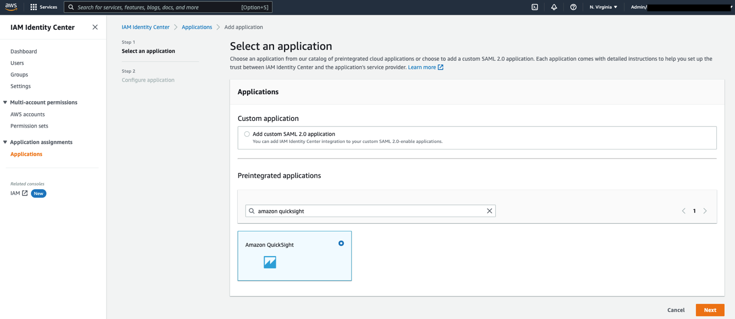
Conclusion

GoDaddy’s hub and spoke data mesh architecture built using Lake Formation simplifies security management and data governance at scale, to deliver data as a service supporting company-wide data accessibility. Our data mesh manages multiple petabytes of data across hundreds of accounts, enabling decentralized ownership of well-defined datasets with automation in place, which helps the business discover data assets quicker and derive business insights faster.

This post illustrates the use of Lake Formation to build a data mesh architecture that enables a DaaS model for a modernized enterprise data platform. For more information, see Design a data mesh architecture using AWS Lake Formation and AWS Glue.


About the Authors

Ankit Jhalaria is the Director Of Engineering on the Data Platform at GoDaddy. He has over 10 years of experience working in big data technologies. Outside of work, Ankit loves hiking, playing board games, building IoT projects, and contributing to open-source projects.

Harsh Vardhan is an AWS Solutions Architect, specializing in Analytics. He has over 6 years of experience working in the field of big data and data science. He is passionate about helping customers adopt best practices and discover insights from their data.

Kyle Tedeschi is a Principal Solutions Architect at AWS. He enjoys helping customers innovate, transform, and become leaders in their respective domains. Outside of work, Kyle is an avid snowboarder, car enthusiast, and traveler.

Use Karpenter to speed up Amazon EMR on EKS autoscaling

Post Syndicated from Changbin Gong original https://aws.amazon.com/blogs/big-data/use-karpenter-to-speed-up-amazon-emr-on-eks-autoscaling/

Amazon EMR on Amazon EKS is a deployment option for Amazon EMR that allows organizations to run Apache Spark on Amazon Elastic Kubernetes Service (Amazon EKS). With EMR on EKS, the Spark jobs run on the Amazon EMR runtime for Apache Spark. This increases the performance of your Spark jobs so that they run faster and cost less than open source Apache Spark. Also, you can run Amazon EMR-based Apache Spark applications with other types of applications on the same EKS cluster to improve resource utilization and simplify infrastructure management.

Karpenter was introduced at AWS re:Invent 2021 to provide a dynamic, high performance, open-source cluster auto scaling solution for Kubernetes. It automatically provisions new nodes in response to unschedulable pods. It observes the aggregate resource requests of unscheduled pods and makes decisions to launch new nodes and terminate stop them to reduce scheduling latencies as well as infrastructure costs.

To configure Karpenter, you create provisioners that define how Karpenter manages the pods that are pending and expires nodes. Although most use cases are addressed with a single provisioner, multiple provisioners are useful in multi-tenant use cases such as isolating nodes for billing, using different node constraints (such as no GPUs for a team), or using different deprovisioning settings. Karpenter launches nodes with minimal compute resources to fit un-schedulable pods for efficient binpacking. It works in tandem with the Kubernetes scheduler to bind un-schedulable pods to the new nodes that are provisioned. The following diagram illustrates how it works.

This post shows how to integrate Karpenter into your EMR on EKS architecture to achieve faster and capacity-aware auto scaling capabilities to speed up your big data and machine learning (ML) workloads while reducing costs. We run the same workload using both Cluster Autoscaler and Karpenter, to see some of the improvements we discuss in the next section.

Improvements compared to Cluster Autoscaler

Like Karpenter, Kubernetes Cluster Autoscaler (CAS) is designed to add nodes when requests come in to run pods that can’t be met by current capacity. Cluster Autoscaler is part of the Kubernetes project, with implementations by major Kubernetes cloud providers. By taking a fresh look at provisioning, Karpenter offers the following improvements:

  • No node group management overhead – Because you have different resource requirements for different Spark workloads along with other workloads in your EKS cluster, you need to create separate node groups that can meet your requirements, like instance sizes, Availability Zones, and purchase options. This can quickly grow to tens and hundreds of node groups, which adds additional management overhead. Karpenter manages each instance directly, without the use of additional orchestration mechanisms like node groups, taking a group-less approach by calling the EC2 Fleet API directly to provision nodes. This allows Karpenter to use diverse instance types, Availability Zones, and purchase options by simply creating a single provisioner, as shown in the following figure.
  • Quick retries – If the Amazon Elastic Compute Cloud (Amazon EC2) capacity isn’t available, Karpenter can retry in milliseconds instead of minutes. This is can be a really useful if you’re using EC2 Spot Instances and you’re unable to get capacity to specific instance types.
  • Designed to handle full flexibility of the cloud – Karpenter has the ability to efficiently address the full range of instance types available through AWS. Cluster Autoscaler wasn’t originally built with the flexibility to handle hundreds of instance types, Availability Zones, and purchase options. We recommend being as flexible as you can be to enable Karpenter get the just-in-time capacity you need.
  • Improves the overall node utilization by binpacking – Karpenter batches pending pods and then binpacks them based on CPU, memory, and GPUs required, taking into account node overhead (for example, daemon set resources required). After the pods are binpacked on the most efficient instance type, Karpenter takes other instance types that are similar or larger than the most efficient packing, and passes the instance type options to an API called EC2 Fleet, following some of the best practices of instance diversification to improve the chances of getting the request capacity.

Best practices using Karpenter with EMR on EKS

For general best practices with Karpenter, refer to Karpenter Best Practices. The following are additional things to consider with EMR on EKS:

  • Avoid inter-AZ data transfer cost by either configuring the Karpenter provisioner to launch in a single Availability Zone or use node selector or affinity and anti-affinity to schedule the driver and the executors of the same job to a single Availability Zone. See the following code:
    nodeSelector:
      topology.kubernetes.io/zone: us-east-1a

  • Cost optimize Spark workloads using EC2 Spot Instances for executors and On-Demand Instances for the driver by using the node selector with the label karpenter.sh/capacity-type in the pod templates. We recommend using pod templates to specify driver pods to run on On-Demand Instances and executor pods to run on Spot Instances. This allows you to consolidate provisioner specs because you don’t need two specs per job type. It also follows the best practice of using customization defined on workload types and to keep provisioner specs to support a broader number of use cases.
  • When using EC2 Spot Instances, maximize the instance diversification in the provisioner configuration to adhere to the best practices. To select suitable instance types, you can use the ec2-instance-selector, a CLI tool and go library that recommends instance types based on resource criteria like vCPUs and memory.

Solution overview

This post provides an example of how to set up both Cluster Autoscaler and Karpenter in an EKS cluster and compare the auto scaling improvements by running a sample EMR on EKS workload.

The following diagram illustrates the architecture of this solution.

We use the Transaction Processing Performance Council-Decision Support (TPC-DS), a decision support benchmark to sequentially run three Spark SQL queries (q70-v2.4, q82-v2.4, q64-v2.4) with a fixed number of 50 executors, against 17.7 billion records, approximately 924 GB compressed data in Parquet file format. For more details on TPC-DS, refer to the eks-spark-benchmark GitHub repo.

We submit the same job with different Spark driver and executor specs to mimic different jobs solely to observe the auto scaling behavior and binpacking. We recommend you right-size your Spark executors based on the workload characteristics for production workloads.

The following code is an example Spark configuration that results in pod spec requests of 4 vCPU and 15 GB:

--conf spark.executor.instances=50 --conf spark.driver.cores=4 --conf spark.driver.memory=10g --conf spark.driver.memoryOverhead=5g --conf spark.executor.cores=4 --conf spark.executor.memory=10g  --conf spark.executor.memoryOverhead=5g

We use pod templates to schedule Spark drivers on On-Demand Instances and executors on EC2 Spot Instances (which can save up to 90% over On-Demand Instance prices). Spark’s inherent resiliency has the driver launch new executors to replace the ones that fail due to Spot interruptions. See the following code:

apiVersion: v1
kind: Pod
spec:
  nodeSelector:
    karpenter.sh/capacity-type: spot
  containers:
  - name: spark-kubernetes-executor


apiVersion: v1
kind: Pod
spec:
  nodeSelector:
    karpenter.sh/capacity-type: on-demand
  containers:
  - name: spark-kubernetes-driver

Prerequisites

We use an AWS Cloud9 IDE to run all the instructions throughout this post.

To create your IDE, run the following commands in AWS CloudShell. The default Region is us-east-1, but you can change it if needed.

# clone the repo
git clone https://github.com/black-mirror-1/karpenter-for-emr-on-eks.git
cd karpenter-for-emr-on-eks
./setup/create-cloud9-ide.sh

Navigate to the AWS Cloud9 IDE using the URL from the output of the script.

Install tools on the AWS Cloud9 IDE

Install the following tools required on the AWS Cloud9 environment by the running a script:

Run the following instructions in your AWS Cloud9 environment and not CloudShell.

  1. Clone the GitHub repository:
    cd ~/environment
    git clone https://github.com/black-mirror-1/karpenter-for-emr-on-eks.git
    cd ~/environment/karpenter-for-emr-on-eks

  2. Set up the required environment variables. Feel free to adjust the following code according to your needs:
    # Install envsubst (from GNU gettext utilities) and bash-completion
    sudo yum -y install jq gettext bash-completion moreutils
    
    # Setup env variables required
    export EKSCLUSTER_NAME=aws-blog
    export EKS_VERSION="1.23"
    # get the link to the same version as EKS from here https://docs.aws.amazon.com/eks/latest/userguide/install-kubectl.html
    export KUBECTL_URL="https://s3.us-west-2.amazonaws.com/amazon-eks/1.23.7/2022-06-29/bin/linux/amd64/kubectl"
    export HELM_VERSION="v3.9.4"
    export KARPENTER_VERSION="v0.18.1"
    # get the most recent matching version of the Cluster Autoscaler from here https://github.com/kubernetes/autoscaler/releases
    export CAS_VERSION="v1.23.1"

  3. Install the AWS Cloud9 CLI tools:
    cd ~/environment/karpenter-for-emr-on-eks
    ./setup/c9-install-tools.sh

Provision the infrastructure

We set up the following resources using the provision infrastructure script:

  1. Create the EMR on EKS and Karpenter infrastructure:
    cd ~/environment/karpenter-for-emr-on-eks
    ./setup/create-eks-emr-infra.sh

  2. Validate the setup:
    # Should have results that are running
    kubectl get nodes
    kubectl get pods -n karpenter
    kubectl get po -n kube-system -l app.kubernetes.io/instance=cluster-autoscaler
    kubectl get po -n prometheus

Understanding Karpenter configurations

Because the sample workload has driver and executor specs that are of different sizes, we have identified the instances from c5, c5a, c5d, c5ad, c6a, m4, m5, m5a, m5d, m5ad, and m6a families of sizes 2xlarge, 4xlarge, 8xlarge, and 9xlarge for our workload using the amazon-ec2-instance-selector CLI. With CAS, we need to create a total of 12 node groups, as shown in eksctl-config.yaml, but can define the same constraints in Karpenter with a single provisioner, as shown in the following code:

apiVersion: karpenter.sh/v1alpha5
kind: Provisioner
metadata:
  name: default
spec:
  provider:
    launchTemplate: {EKSCLUSTER_NAME}-karpenter-launchtemplate
    subnetSelector:
      karpenter.sh/discovery: {EKSCLUSTER_NAME}
  labels:
    app: kspark
  requirements:
    - key: "karpenter.sh/capacity-type"
      operator: In
      values: ["on-demand","spot"]
    - key: "kubernetes.io/arch" 
      operator: In
      values: ["amd64"]
    - key: karpenter.k8s.aws/instance-family
      operator: In
      values: [c5, c5a, c5d, c5ad, m5, c6a]
    - key: karpenter.k8s.aws/instance-size
      operator: In
      values: [2xlarge, 4xlarge, 8xlarge, 9xlarge]
    - key: "topology.kubernetes.io/zone"
      operator: In
      values: ["{AWS_REGION}a"]

  limits:
    resources:
      cpu: "2000"

  ttlSecondsAfterEmpty: 30

We have set up both auto scalers to scale down nodes that are empty for 30 seconds using ttlSecondsAfterEmpty in Karpenter and --scale-down-unneeded-time in CAS.

Karpenter by design will try to achieve the most efficient packing of the pods on a node based on CPU, memory, and GPUs required.

Run a sample workload

To run a sample workload, complete the following steps:

  1. Lets review the AWS Command Line Interface (AWS CLI) command to submit a sample job:
    aws emr-containers start-job-run \
      --virtual-cluster-id $VIRTUAL_CLUSTER_ID \
      --name karpenter-benchmark-${CORES}vcpu-${MEMORY}gb  \
      --execution-role-arn $EMR_ROLE_ARN \
      --release-label emr-6.5.0-latest \
      --job-driver '{
      "sparkSubmitJobDriver": {
          "entryPoint": "local:///usr/lib/spark/examples/jars/eks-spark-benchmark-assembly-1.0.jar",
          "entryPointArguments":["s3://blogpost-sparkoneks-us-east-1/blog/BLOG_TPCDS-TEST-3T-partitioned","s3://'$S3BUCKET'/EMRONEKS_TPCDS-TEST-3T-RESULT-KA","/opt/tpcds-kit/tools","parquet","3000","1","false","q70-v2.4,q82-v2.4,q64-v2.4","true"],
          "sparkSubmitParameters": "--class com.amazonaws.eks.tpcds.BenchmarkSQL --conf spark.executor.instances=50 --conf spark.driver.cores='$CORES' --conf spark.driver.memory='$EXEC_MEMORY'g --conf spark.executor.cores='$CORES' --conf spark.executor.memory='$EXEC_MEMORY'g"}}' \
      --configuration-overrides '{
        "applicationConfiguration": [
          {
            "classification": "spark-defaults", 
            "properties": {
              "spark.kubernetes.node.selector.app": "kspark",
              "spark.kubernetes.node.selector.topology.kubernetes.io/zone": "'${AWS_REGION}'a",
    
              "spark.kubernetes.container.image":  "'$ECR_URL'/eks-spark-benchmark:emr6.5",
              "spark.kubernetes.driver.podTemplateFile": "s3://'$S3BUCKET'/pod-template/karpenter-driver-pod-template.yaml",
              "spark.kubernetes.executor.podTemplateFile": "s3://'$S3BUCKET'/pod-template/karpenter-executor-pod-template.yaml",
              "spark.network.timeout": "2000s",
              "spark.executor.heartbeatInterval": "300s",
              "spark.kubernetes.executor.limit.cores": "'$CORES'",
              "spark.executor.memoryOverhead": "'$MEMORY_OVERHEAD'G",
              "spark.driver.memoryOverhead": "'$MEMORY_OVERHEAD'G",
              "spark.kubernetes.executor.podNamePrefix": "karpenter-'$CORES'vcpu-'$MEMORY'gb",
              "spark.executor.defaultJavaOptions": "-verbose:gc -XX:+UseG1GC",
              "spark.driver.defaultJavaOptions": "-verbose:gc -XX:+UseG1GC",
    
              "spark.ui.prometheus.enabled":"true",
              "spark.executor.processTreeMetrics.enabled":"true",
              "spark.kubernetes.driver.annotation.prometheus.io/scrape":"true",
              "spark.kubernetes.driver.annotation.prometheus.io/path":"/metrics/executors/prometheus/",
              "spark.kubernetes.driver.annotation.prometheus.io/port":"4040",
              "spark.kubernetes.driver.service.annotation.prometheus.io/scrape":"true",
              "spark.kubernetes.driver.service.annotation.prometheus.io/path":"/metrics/driver/prometheus/",
              "spark.kubernetes.driver.service.annotation.prometheus.io/port":"4040",
              "spark.metrics.conf.*.sink.prometheusServlet.class":"org.apache.spark.metrics.sink.PrometheusServlet",
              "spark.metrics.conf.*.sink.prometheusServlet.path":"/metrics/driver/prometheus/",
              "spark.metrics.conf.master.sink.prometheusServlet.path":"/metrics/master/prometheus/",
              "spark.metrics.conf.applications.sink.prometheusServlet.path":"/metrics/applications/prometheus/"
             }}
        ]}'

  2. Submit four jobs with different driver and executor vCPUs and memory sizes on Karpenter:
    # the arguments are vcpus and memory
    export EMRCLUSTER_NAME=${EKSCLUSTER_NAME}-emr
    ./sample-workloads/emr6.5-tpcds-karpenter.sh 4 7
    ./sample-workloads/emr6.5-tpcds-karpenter.sh 8 15
    ./sample-workloads/emr6.5-tpcds-karpenter.sh 4 15
    ./sample-workloads/emr6.5-tpcds-karpenter.sh 8 31 

  3. To monitor the pods’s autoscaling status in real time, open a new terminal in Cloud9 IDE and run the following command (nothing is returned at the start):
    watch -n1 "kubectl get pod -n emr-karpenter"

  4. Observe the EC2 instance and node auto scaling status in a second terminal tab by running the following command (by design, Karpenter schedules in Availability Zone a):
    watch -n1 "kubectl get node --label-columns=node.kubernetes.io/instance-type,karpenter.sh/capacity-type,topology.kubernetes.io/zone,app -l app=kspark"

Compare with Cluster Autoscaler (Optional)

We have set up Cluster Autoscaler during the infrastructure setup step with the following configuration:

  • Launch EC2 nodes in Availability Zone b
  • Contain 12 node groups (6 each for On-Demand and Spot)
  • Scale down unneeded nodes after 30 seconds with --scale-down-unneeded-time
  • Use the least-waste expander on CAS, which can select the node group that will have the least idle CPU for binpacking efficiency
  1. Submit four jobs with different driver and executor vCPUs and memory sizes on CAS:
    # the arguments are vcpus and memory
    ./sample-workloads/emr6.5-tpcds-ca.sh 4 7
    ./sample-workloads/emr6.5-tpcds-ca.sh 8 15
    ./sample-workloads/emr6.5-tpcds-ca.sh 4 15
    ./sample-workloads/emr6.5-tpcds-ca.sh 8 31

  2. To monitor the pods’s autoscaling status in real time, open a new terminal in Cloud9 IDE and run the following command (nothing is returned at the start):
    watch -n1 "kubectl get pod -n emr-ca"

  3. Observe the EC2 instance and node auto scaling status in a second terminal tab by running the following command (by design, CAS schedules in Availability Zone b):
    watch -n1 "kubectl get node --label-columns=node.kubernetes.io/instance-type,eks.amazonaws.com/capacityType,topology.kubernetes.io/zone,app -l app=caspark"

Observations

The time from pod creation to being scheduled on average is less with Karpenter than CAS, as shown in the following figure; you can see a noticeable difference when you run large scale workloads.

As shown in the following figures, as the jobs were completed, Karpenter was able to scale down the nodes that aren’t needed within seconds. In contrast, CAS takes minutes, because it sends a signal to the node groups, adding additional latency. This in turn helps reduce overall costs by reducing the number of seconds unneeded EC2 instances are running.

Clean up

To clean up your environment, delete all the resources created in reverse order by running the cleanup script:

export EKSCLUSTER_NAME=aws-blog
cd ~/environment/karpenter-for-emr-on-eks
./setup/cleanup.sh

Conclusion

In this post, we showed you how to use Karpenter to simplify EKS node provisioning, and speed up auto scaling of EMR on EKS workloads. We encourage you to try Karpenter and provide any feedback by creating a GitHub issue.

Further reading


About the Authors

Changbin Gong is a Principal Solutions Architect at Amazon Web Services. He engages with customers to create innovative solutions that address customer business problems and accelerate the adoption of AWS services. In his spare time, Changbin enjoys reading, running, and traveling.

Sandeep Palavalasa is a Sr. Specialist Containers SA at Amazon Web Services. He is a software technology leader with over 12 years of experience in building large-scale, distributed software systems. His professional career started with a focus on monitoring and observability and he has a strong cloud architecture background. He likes working on distributed systems and is excited to talk about microservice architecture design. His current interests are in the areas of container services and serverless technologies.

Use an event-driven architecture to build a data mesh on AWS

Post Syndicated from Jan Michael Go Tan original https://aws.amazon.com/blogs/big-data/use-an-event-driven-architecture-to-build-a-data-mesh-on-aws/

In this post, we take the data mesh design discussed in Design a data mesh architecture using AWS Lake Formation and AWS Glue, and demonstrate how to initialize data domain accounts to enable managed sharing; we also go through how we can use an event-driven approach to automate processes between the central governance account and data domain accounts (producers and consumers). We build a data mesh pattern from scratch as Infrastructure as Code (IaC) using AWS CDK and use an open-source self-service data platform UI to share and discover data between business units.

The key advantage of this approach is being able to add actions in response to data mesh events such as permission management, tag propagation, search index management, and to automate different processes.

Before we dive into it, let’s look at AWS Analytics Reference Architecture, an open-source library that we use to build our solution.

AWS Analytics Reference Architecture

AWS Analytics Reference Architecture (ARA) is a set of analytics solutions put together as end-to-end examples. It regroups AWS best practices for designing, implementing, and operating analytics platforms through different purpose-built patterns, handling common requirements, and solving customers’ challenges.

ARA exposes reusable core components in an AWS CDK library, currently available in Typescript and Python. This library contains AWS CDK constructs (L3) that can be used to quickly provision analytics solutions in demos, prototypes, proofs of concept, and end-to-end reference architectures.

The following table lists data mesh specific constructs in the AWS Analytics Reference Architecture library.

Construct Name Purpose
CentralGovernance Creates an Amazon EventBridge event bus for central governance account that is used to communicate with data domain accounts (producer/consumer). Creates workflows to automate data product registration and sharing.
DataDomain Creates an Amazon EventBridge event bus for data domain account (producer/consumer) to communicate with central governance account. It creates data lake storage (Amazon S3), and workflow to automate data product registration. It also creates a workflow to populate AWS Glue Catalog metadata for newly registered data product.

You can find AWS CDK constructs for the AWS Analytics Reference Architecture on Construct Hub.

In addition to ARA constructs, we also use an open-source Self-service data platform (User Interface). It is built using AWS Amplify, Amazon DynamoDB, AWS Step Functions, AWS Lambda, Amazon API Gateway, Amazon EventBridge, Amazon Cognito, and Amazon OpenSearch. The frontend is built with React. Through the self-service data platform you can: 1) manage data domains and data products, and 2) discover and request access to data products.

Central Governance and data sharing

For the governance of our data mesh, we will use AWS Lake Formation. AWS Lake Formation is a fully managed service that simplifies data lake setup, supports centralized security management, and provides transactional access on top of your data lake. Moreover, it enables data sharing across accounts and organizations. This centralized approach has a number of key benefits, such as: centralized audit; centralized permission management; and centralized data discovery. More importantly, this allows organizations to gain the benefits of centralized governance while taking advantage of the inherent scaling characteristics of decentralized data product management.

There are two ways to share data resources in Lake Formation: 1) Named Based Access Control (NRAC), and 2) Tag-Based Access Control (LF-TBAC). NRAC uses AWS Resource Access Manager (AWS RAM) to share data resources across accounts. Those are consumed via resource links that are based on created resource shares. Tag-Based Access Control (LF-TBAC) is another approach to share data resources in AWS Lake Formation, that defines permissions based on attributes. These attributes are called LF-tags. You can read this blog to learn about LF-TBAC in the context of data mesh.

The following diagram shows how NRAC and LF-TBAC data sharing works. In this example, data domain is registered as a node on mesh and therefore we create two databases in the central governance account. NRAC database is shared with data domain via AWS RAM. Access to data products that we register in this database will be handled through NRAC. LF-TBAC database is tagged with data domain N line of business (LOB) LF-tag: <LOB:N>. LOB tag is automatically shared with data domain N account and therefore database is available in that account. Access to Data Products in this database will be handled through LF-TBAC.

BDB-2279-ram-tag-share

In our solution we will demonstrate both NRAC and LF-TBAC approaches. With the NRAC approach, we will build up an event-based workflow that would automatically accept RAM share in the data domain accounts and automate the creation of the necessary metadata objects (eg. local database, resource links, etc). While with the LF-TBAC approach, we rely on permissions associated with the shared LF-Tags to allow producer data domains to manage their data products, and consumer data domains read access to the relevant data products associated with the LF-Tags that they requested access to.

We use CentralGovernance construct from ARA library to build a central governance account. It creates an EventBridge event bus to enable communication with data domain accounts that register as nodes on mesh. For each registered data domain, specific event bus rules are created that route events towards that account. Central governance account has a central metadata catalog that allows for data to be stored in different data domains, as opposed to a single central lake. For each registered data domain, we create two separate databases in central governance catalog to demonstrate both NRAC and LF-TBAC data sharing. CentralGovernance construct creates workflows for data product registration and data product sharing. We also deploy a self-service data platform UI  to enable good user experience to manage data domains, data products, and to simplify data discovery and sharing.

BDB-2279-central-gov

A data domain: producer and consumer

We use DataDomain construct from ARA library to build a data domain account that can be either producer, consumer, or both. Producers manage the lifecycle of their respective data products in their own AWS accounts. Typically, this data is stored in Amazon Simple Storage Service (Amazon S3). DataDomain construct creates a data lake storage with cross-account bucket policy that enables central governance account to access the data. Data is encrypted using AWS KMS, and central governance account has a permission to use the key. Config secret in AWS Secrets Manager contains all the necessary information to register data domain as a node on mesh in central governance. It includes: 1) data domain name, 2) S3 location that holds data products, and 3) encryption key ARN. DataDomain construct also creates data domain and crawler workflows to automate data product registration.

BDB-2279-data-domain

Creating an event-driven data mesh

Data mesh architectures typically require some level of communication and trust policy management to maintain least privileges of the relevant principals between the different accounts (for example, central governance to producer, central governance to consumer). We use event-driven approach via EventBridge to securely forward events from one event bus to event bus in another account while maintaining the least privilege access. When we register data domain to central governance account through the self-service data platform UI, we establish bi-directional communication between the accounts via EventBridge. Domain registration process also creates database in the central governance catalog to hold data products for that particular domain. Registered data domain is now a node on mesh and we can register new data products.

The following diagram shows data product registration process:

BDB-2279-register-dd-small

  1. Starts Register Data Product workflow that creates an empty table (the schema is managed by the producers in their respective producer account). This workflow also grants a cross-account permission to the producer account that allows producer to manage the schema of the table.
  2. When complete, this emits an event into the central event bus.
  3. The central event bus contains a rule that forwards the event to the producer’s event bus. This rule was created during the data domain registration process.
  4. When the producer’s event bus receives the event, it triggers the Data Domain workflow, which creates resource-links and grants permissions.
  5. Still in the producer account, Crawler workflow gets triggered when the Data Domain workflow state changes to Successful. This creates the crawler, runs it, waits and checks if the crawler is done, and deletes the crawler when it’s complete. This workflow is responsible for populating tables’ schemas.

Now other data domains can find newly registered data products using the self-service data platform UI and request access. The sharing process works in the same way as product registration by sending events from the central governance account to consumer data domain, and triggering specific workflows.

Solution Overview

The following high-level solution diagram shows how everything fits together and how event-driven architecture enables multiple accounts to form a data mesh. You can follow the workshop that we released to deploy the solution that we covered in this blog post. You can deploy multiple data domains and test both data registration and data sharing. You can also use self-service data platform UI to search through data products and request access using both LF-TBAC and NRAC approaches.

BDB-2279-arch-diagram

Conclusion

Implementing a data mesh on top of an event-driven architecture provides both flexibility and extensibility. A data mesh by itself has several moving parts to support various functionalities, such as onboarding, search, access management and sharing, and more. With an event-driven architecture, we can implement these functionalities in smaller components to make them easier to test, operate, and maintain. Future requirements and applications can use the event stream to provide their own functionality, making the entire mesh much more valuable to your organization.

To learn more how to design and build applications based on event-driven architecture, see the AWS Event-Driven Architecture page. To dive deeper into data mesh concepts, see the Design a Data Mesh Architecture using AWS Lake Formation and AWS Glue blog.

If you’d like our team to run data mesh workshop with you, please reach out to your AWS team.


About the authors


Jan Michael Go Tan is a Principal Solutions Architect for Amazon Web Services. He helps customers design scalable and innovative solutions with the AWS Cloud.

Dzenan Softic is a Senior Solutions Architect at AWS. He works with startups to help them define and execute their ideas. His main focus is in data engineering and infrastructure.

David Greenshtein is a Specialist Solutions Architect for Analytics at AWS with a passion for ETL and automation. He works with AWS customers to design and build analytics solutions enabling business to make data-driven decisions. In his free time, he likes jogging and riding bikes with his son.
Vincent Gromakowski is an Analytics Specialist Solutions Architect at AWS where he enjoys solving customers’ analytics, NoSQL, and streaming challenges. He has a strong expertise on distributed data processing engines and resource orchestration platform.

Simplifying Amazon EC2 instance type flexibility with new attribute-based instance type selection features

Post Syndicated from Sheila Busser original https://aws.amazon.com/blogs/compute/simplifying-amazon-ec2-instance-type-flexibility-with-new-attribute-based-instance-type-selection-features/

This blog is written by Rajesh Kesaraju, Sr. Solution Architect, EC2-Flexible Compute and Peter Manastyrny, Sr. Product Manager, EC2.

Today AWS is adding two new attributes for the attribute-based instance type selection (ABS) feature to make it even easier to create and manage instance type flexible configurations on Amazon EC2. The new network bandwidth attribute allows customers to request instances based on the network requirements of their workload. The new allowed instance types attribute is useful for workloads that have some instance type flexibility but still need more granular control over which instance types to run on.

The two new attributes are supported in EC2 Auto Scaling Groups (ASG), EC2 Fleet, Spot Fleet, and Spot Placement Score.

Before exploring the new attributes in detail, let us review the core ABS capability.

ABS refresher

ABS lets you express your instance type requirements as a set of attributes, such as vCPU, memory, and storage when provisioning EC2 instances with ASG, EC2 Fleet, or Spot Fleet. Your requirements are translated by ABS to all matching EC2 instance types, simplifying the creation and maintenance of instance type flexible configurations. ABS identifies the instance types based on attributes that you set in ASG, EC2 Fleet, or Spot Fleet configurations. When Amazon EC2 releases new instance types, ABS will automatically consider them for provisioning if they match the selected attributes, removing the need to update configurations to include new instance types.

ABS helps you to shift from an infrastructure-first to an application-first paradigm. ABS is ideal for workloads that need generic compute resources and do not necessarily require the hardware differentiation that the Amazon EC2 instance type portfolio delivers. By defining a set of compute attributes instead of specific instance types, you allow ABS to always consider the broadest and newest set of instance types that qualify for your workload. When you use EC2 Spot Instances to optimize your costs and save up to 90% compared to On-Demand prices, instance type diversification is the key to access the highest amount of Spot capacity. ABS provides an easy way to configure and maintain instance type flexible configurations to run fault-tolerant workloads on Spot Instances.

We recommend ABS as the default compute provisioning method for instance type flexible workloads including containerized apps, microservices, web applications, big data, and CI/CD.

Now, let us dive deep on the two new attributes: network bandwidth and allowed instance types.

How network bandwidth attribute for ABS works

Network bandwidth attribute allows customers with network-sensitive workloads to specify their network bandwidth requirements for compute infrastructure. Some of the workloads that depend on network bandwidth include video streaming, networking appliances (e.g., firewalls), and data processing workloads that require faster inter-node communication and high-volume data handling.

The network bandwidth attribute uses the same min/max format as other ABS attributes (e.g., vCPU count or memory) that assume a numeric value or range (e.g., min: ‘10’ or min: ‘15’; max: ‘40’). Note that setting the minimum network bandwidth does not guarantee that your instance will achieve that network bandwidth. ABS will identify instance types that support the specified minimum bandwidth, but the actual bandwidth of your instance might go below the specified minimum at times.

Two important things to remember when using the network bandwidth attribute are:

  • ABS will only take burst bandwidth values into account when evaluating maximum values. When evaluating minimum values, only the baseline bandwidth will be considered.
    • For example, if you specify the minimum bandwidth as 10 Gbps, instances that have burst bandwidth of “up to 10 Gbps” will not be considered, as their baseline bandwidth is lower than the minimum requested value (e.g., m5.4xlarge is burstable up to 10 Gbps with a baseline bandwidth of 5 Gbps).
    • Alternatively, c5n.2xlarge, which is burstable up to 25 Gbps with a baseline bandwidth of 10 Gbps will be considered because its baseline bandwidth meets the minimum requested value.
  • Our recommendation is to only set a value for maximum network bandwidth if you have specific requirements to restrict instances with higher bandwidth. That would help to ensure that ABS considers the broadest possible set of instance types to choose from.

Using the network bandwidth attribute in ASG

In this example, let us look at a high-performance computing (HPC) workload or similar network bandwidth sensitive workload that requires a high volume of inter-node communications. We use ABS to select instances that have at minimum 10 Gpbs of network bandwidth and at least 32 vCPUs and 64 GiB of memory.

To get started, you can create or update an ASG or EC2 Fleet set up with ABS configuration and specify the network bandwidth attribute.

The following example shows an ABS configuration with network bandwidth attribute set to a minimum of 10 Gbps. In this example, we do not set a maximum limit for network bandwidth. This is done to remain flexible and avoid restricting available instance type choices that meet our minimum network bandwidth requirement.

Create the following configuration file and name it: my_asg_network_bandwidth_configuration.json

{
    "AutoScalingGroupName": "network-bandwidth-based-instances-asg",
    "DesiredCapacityType": "units",
    "MixedInstancesPolicy": {
        "LaunchTemplate": {
            "LaunchTemplateSpecification": {
                "LaunchTemplateName": "LaunchTemplate-x86",
                "Version": "$Latest"
            },
            "Overrides": [
                {
                "InstanceRequirements": {
                    "VCpuCount": {"Min": 32},
                    "MemoryMiB": {"Min": 65536},
                    "NetworkBandwidthGbps": {"Min": 10} }
                 }
            ]
        },
        "InstancesDistribution": {
            "OnDemandPercentageAboveBaseCapacity": 30,
            "SpotAllocationStrategy": "capacity-optimized"
        }
    },
    "MinSize": 1,
    "MaxSize": 10,
    "DesiredCapacity":10,
    "VPCZoneIdentifier": "subnet-f76e208a, subnet-f76e208b, subnet-f76e208c"
}

Next, let us create an ASG using the following command:

my_asg_network_bandwidth_configuration.json file

aws autoscaling create-auto-scaling-group --cli-input-json file://my_asg_network_bandwidth_configuration.json

As a result, you have created an ASG that may include instance types m5.8xlarge, m5.12xlarge, m5.16xlarge, m5n.8xlarge, and c5.9xlarge, among others. The actual selection at the time of the request is made by capacity optimized Spot allocation strategy. If EC2 releases an instance type in the future that would satisfy the attributes provided in the request, that instance will also be automatically considered for provisioning.

Considered Instances (not an exhaustive list)


Instance Type        Network Bandwidth
m5.8xlarge             “10 Gbps”

m5.12xlarge           “12 Gbps”

m5.16xlarge           “20 Gbps”

m5n.8xlarge          “25 Gbps”

c5.9xlarge               “10 Gbps”

c5.12xlarge             “12 Gbps”

c5.18xlarge             “25 Gbps”

c5n.9xlarge            “50 Gbps”

c5n.18xlarge          “100 Gbps”

…

Now let us focus our attention on another new attribute – allowed instance types.

How allowed instance types attribute works in ABS

As discussed earlier, ABS lets us provision compute infrastructure based on our application requirements instead of selecting specific EC2 instance types. Although this infrastructure agnostic approach is suitable for many workloads, some workloads, while having some instance type flexibility, still need to limit the selection to specific instance families, and/or generations due to reasons like licensing or compliance requirements, application performance benchmarking, and others. Furthermore, customers have asked us to provide the ability to restrict the auto-consideration of newly released instances types in their ABS configurations to meet their specific hardware qualification requirements before considering them for their workload. To provide this functionality, we added a new allowed instance types attribute to ABS.

The allowed instance types attribute allows ABS customers to narrow down the list of instance types that ABS considers for selection to a specific list of instances, families, or generations. It takes a comma separated list of specific instance types, instance families, and wildcard (*) patterns. Please note, that it does not use the full regular expression syntax.

For example, consider container-based web application that can only run on any 5th generation instances from compute optimized (c), general purpose (m), or memory optimized (r) families. It can be specified as “AllowedInstanceTypes”: [“c5*”, “m5*”,”r5*”].

Another example could be to limit the ABS selection to only memory-optimized instances for big data Spark workloads. It can be specified as “AllowedInstanceTypes”: [“r6*”, “r5*”, “r4*”].

Note that you cannot use both the existing exclude instance types and the new allowed instance types attributes together, because it would lead to a validation error.

Using allowed instance types attribute in ASG

Let us look at the InstanceRequirements section of an ASG configuration file for a sample web application. The AllowedInstanceTypes attribute is configured as [“c5.*”, “m5.*”,”c4.*”, “m4.*”] which means that ABS will limit the instance type consideration set to any instance from 4th and 5th generation of c or m families. Additional attributes are defined to a minimum of 4 vCPUs and 16 GiB RAM and allow both Intel and AMD processors.

Create the following configuration file and name it: my_asg_allow_instance_types_configuration.json

{
    "AutoScalingGroupName": "allow-instance-types-based-instances-asg",
    "DesiredCapacityType": "units",
    "MixedInstancesPolicy": {
        "LaunchTemplate": {
            "LaunchTemplateSpecification": {
                "LaunchTemplateName": "LaunchTemplate-x86",
                "Version": "$Latest"
            },
            "Overrides": [
                {
                "InstanceRequirements": {
                    "VCpuCount": {"Min": 4},
                    "MemoryMiB": {"Min": 16384},
                    "CpuManufacturers": ["intel","amd"],
                    "AllowedInstanceTypes": ["c5.*", "m5.*","c4.*", "m4.*"] }
            }
            ]
        },
        "InstancesDistribution": {
            "OnDemandPercentageAboveBaseCapacity": 30,
            "SpotAllocationStrategy": "capacity-optimized"
        }
    },
    "MinSize": 1,
    "MaxSize": 10,
    "DesiredCapacity":10,
    "VPCZoneIdentifier": "subnet-f76e208a, subnet-f76e208b, subnet-f76e208c"
}

As a result, you have created an ASG that may include instance types like m5.xlarge, m5.2xlarge, c5.xlarge, and c5.2xlarge, among others. The actual selection at the time of the request is made by capacity optimized Spot allocation strategy. Please note that if EC2 will in the future release a new instance type which will satisfy the other attributes provided in the request, but will not be a member of 4th or 5th generation of m or c families specified in the allowed instance types attribute, the instance type will not be considered for provisioning.

Selected Instances (not an exhaustive list)

m5.xlarge

m5.2xlarge

m5.4xlarge

…

c5.xlarge

c5.2xlarge

…

m4.xlarge

m4.2xlarge

m4.4xlarge

…

c4.xlarge

c4.2xlarge

…

As you can see, ABS considers a broad set of instance types for provisioning, however they all meet the compute attributes that are required for your workload.

Cleanup

To delete both ASGs and terminate all the instances, execute the following commands:

aws autoscaling delete-auto-scaling-group --auto-scaling-group-name network-bandwidth-based-instances-asg --force-delete

aws autoscaling delete-auto-scaling-group --auto-scaling-group-name allow-instance-types-based-instances-asg --force-delete

Conclusion

In this post, we explored the two new ABS attributes – network bandwidth and allowed instance types. Customers can use these attributes to select instances based on network bandwidth and to limit the set of instances that ABS selects from. The two new attributes, as well as the existing set of ABS attributes enable you to save time on creating and maintaining instance type flexible configurations and make it even easier to express the compute requirements of your workload.

ABS represents the paradigm shift in the way that our customers interact with compute, making it easier than ever to request diversified compute resources at scale. We recommend ABS as a tool to help you identify and access the largest amount of EC2 compute capacity for your instance type flexible workloads.

Publish Amazon DevOps Guru Insights to Slack Channel

Post Syndicated from Chetan Makvana original https://aws.amazon.com/blogs/devops/publish-amazon-devops-guru-insights-to-slack-channel/

Customers using Amazon DevOps Guru often wants to publish operational insights to chat collaboration platforms, such as Slack and Amazon Chime. Amazon DevOps Guru offers a fully managed AIOps platform service that enables developers and operators to improve application availability and resolve operational issues faster. It minimizes manual effort by leveraging machine learning (ML) powered recommendations. DevOps Guru automatically detects operational insights, predicts impending resource exhaustion, details likely cause, and recommends remediation actions. For customers running critical applications, having access to these operational insights and real-time alerts are key aspects to improve their overall incident remediation processes and maintain operational excellence. Customers use chat collaboration platforms to monitor operational insights and respond to events, which reduces context switching between applications and provides opportunities to respond faster.

This post walks you through how to integrate DevOps Guru with Slack channel to receive notifications for new operational insights detected by DevOps Guru. It doesn’t talk about enabling Amazon DevOps Guru and generating operational insights. You can refer to Gaining operational insights with AIOps using Amazon DevOps Guru to know more about this.

Solution overview

Amazon DevOps Guru integrates with Amazon EventBridge to notify you of events relating to insights and corresponding insight updates. To receive operational insight notifications in Slack channels, you configure routing rules to determine where to send notifications and use pre-defined DevOps Guru patterns to only send notifications or trigger actions that match that pattern. You can select any of the following pre-defined patterns to filter events to trigger actions in a supported AWS resource. For this post, we will send events only for “New Insights Open”.

  • DevOps Guru New Insight Open
  • DevOps Guru New Anomaly Association
  • DevOps Guru Insight Severity Upgraded
  • DevOps Guru New Recommendation Created
  • DevOps Guru Insight Closed

When EventBridge receives an event from DevOps Guru, the event rule fires and the event notification is sent to Slack channel by using AWS Lambda or AWS Chatbot. Chatbot is easier to configure and deploy. However, if you want more customization, we have also written a Lambda function that allows additional formatting options.

Amazon EventBridge receives an event from Amazon DevOps Guru, and fires event rule. A rule matches incoming events and sends them to AWS Lambda or AWS Chatbot. With AWS Lambda, you write code to customize the message and send formatted message to the Slack channel. To receive event notifications in chat channels, you configure an SNS topic as a target in the Amazon EventBridge rule and then associate the topic with a chat channel in the AWS Chatbot console. AWS Chatbot then sends event to the configured Slack channel.

Figure 1: Amazon EventBridge Integration with Slack using AWS Lambda or AWS Chatbot

The goal of this tutorial is to show a technical walkthrough of integration of DevOps Guru with Slack using the following options:

  1. Publish using AWS Lambda
  2. Publish using AWS Chatbot

Prerequisites

For this walkthrough, you should have the following prerequisites:

Publish using AWS Lambda

In this tutorial, you will perform the following steps:

  • Create a Slack Webhook URL
  • Launch SAM template to deploy the solution
  • Test the solution

Create a Slack Webhook URL

This step configures Slack workflow and creates a Webhook URL used for API call. You will need to have access to add a new channel and app to your Slack Workspace.

  1. Create a new channel for events (i.e. devopsguru_events).
  2. Within Slack, click on your workspace name drop-down arrow in the upper left.
  3. Choose Tools > Workflow Builder.
  4. Click Create in the upper right-hand corner of the Workflow Builder and give your workflow a name.
  5. Click Next.
  6. Click Select next to Webhook.
  7. Click Add variable and add the following variables one at a time in the Key section. All data types will be text.
    • text
    • account
    • region
    • startTime
    • insightType
    • severity
    • description
    • insightUrl
    • numOfAnomalies
  1. When done, you should have 9 variables, double check them as they are case sensitive and will be referenced.
  2. Click Add Step.
  3. On the Add a workflow step window, click Add next to send a message.
  4. Under Send this message to select the channel you created in earlier step.
  5. In Message text, create the following.
Final message is with placeholder as corresponding variables created in Step #7

Figure 2: Message text configuration in Slack

  1. Click Save.
  2. Click Publish.
  3. For the deployment, we will need the Webhook URL. Copy it in the notepad.

Launch SAM template to deploy the solution

In this step, you will launch the SAM template. This template deploys an AWS Lambda function that is triggered by an Amazon EventBridge rule when Amazon DevOps Guru notifies event relating to “DevOps Guru New Insight Open”. It also deploys AWS Secret Manager, Amazon EventBridge Rule and required permission to invoke this specific function. The AWS Lambda function retrieves the Slack Webhook URL from AWS Secret Manager and posts a message to Slack using webhook API call.

  1. Create a new directory, navigate to that directory in a terminal and clone the GitHub repository using the below command.
  1. Change directory to the directory where you cloned the GitHub repository.
cd devops-guru-integration-with-slack
  1. From the command line, use AWS SAM to build the serverless application with its dependencies.
sam build
  1. From the command line, use AWS SAM to deploy the AWS resources for the pattern as specified in the template.yml file.
sam deploy --guided
  1. During the prompts.
    • enter a stack name.
    • enter the desired AWS Region.
    • enter the Secret name to store Slack Channel Webhook URL.
    • enter the Slack Channel Webhook URL that you copied in an earlier step.
    • allow SAM CLI to create IAM roles with the required permissions.

Once you have run sam deploy --guided mode once and saved arguments to a configuration file (samconfig.toml), you can use sam deploy in future to use these defaults.

Test the solution

  1. Follow this blog to enable DevOps Guru and generate operational insights.
  2. When DevOps Guru detects a new insight, it generates events in EventBridge. EventBridge then triggers Lambda that sends it to a Slack channel as below.
Slack channel shows message with details like Account, Region, Start Time, Insight Type, Severity, Description, Insight URL and Number of anomalies found.

Figure 3. Message published to Slack

Cleaning up

To avoid incurring future charges, delete the resources.

  1. Delete resources deployed from this blog.
  2. From the command line, use AWS SAM to delete the serverless application with its dependencies.
sam delete

Publish using AWS Chatbot

In this tutorial, you will perform the following steps:

  • Configure Amazon Simple Notification Service (SNS) and Amazon EventBridge using the AWS Command Line Interface (CLI)
  • Configure AWS Chatbot to a Slack workspace
  • Test the solution

Configure Amazon SNS and Amazon Eventbridge

We will now configure and deploy an SNS topic and an Eventbridge rule. This EventBridge rule will be triggered by DevOps Guru when “DevOps Guru New Insight Open” events are generated. The event will then be sent to the SNS topic which we will configure as a target for the Eventbridge rule.

  1. Using CLI, create an SNS topic running the following command in the CLI. Alternatively, you can configure and create an SNS topic in the AWS management console.
aws sns create-topic --name devops-guru-insights-chatbot-topic
  1. Save the SNS topic ARN that is generated in the CLI for a later step in this walkthrough.
  2. Now we will create the Eventbridge rule. Run the following command to create the Eventbridge rule. Alternatively, you can configure and create the rule in the AWS management console.
aws events put-rule --name "devops-guru-insights-chatbot-rule" -
-event-pattern "{\"source\":[\"aws.devops-guru\"],\"detail-type\":[\"DevOps
 Guru New Insight Open\"]}"
  1. We now want to add targets to the rule we just created. Use the ARN of the SNS topic we created in step one.
aws events put-targets --rule devops-guru-insights-chatbot-rule --targets "Id"="1","Arn"=""
  1. We now have created an SNS topic, and an Eventbridge rule to send “DevOps Guru New Insight Open” events to that SNS topic.

Create and Add AWS Chatbot to a Slack workspace

In this step, we will configure AWS Chatbot and our Slack channel to receive the SNS Notifications we configured in the previous step.

  1. Sign into the AWS management console and open AWS Chatbot at https://console.aws.amazon.com/Chatbot/.
  2. Under Configure a chat client, select Slack from the dropdown and click Configure Client.
  3. You will then need to give AWS Chatbot permission to access your workspace, click Allow.
AWS Chatbot is requesting permission to access the Slack workspace

Figure 4.  AWS Chatbot requesting permission

  1. Once configured, you’ll be redirected to the AWS management console. You’ll now want to click Configure new channel.
  2. Use the follow configurations for the setup of the Slack channel.
    • Configuration Name: aws-chatbot-devops-guru
    • Channel Type: Public or Private
      • If adding Chatbot to a private channel, you will need the Channel ID. One way you can get this is by going to your slack channel and copying the link, the last set of unique characters will be your Channel ID.
    • Channel Role: Create an IAM role using a template
    • Role name: awschatbot-devops-guru-role
    • Policy templates: Notification permissions
    • Guardrail Policies: AWS-Chatbot-NotificationsOnly-Policy-5f5dfd95-d198-49b0-8594-68d08aba8ba1
    • SNS Topics:
      • Region: us-east-1 (Select the region you created the SNS topic in)
      • Topics: devops-guru-insights-chatbot-topic
  1.  Click Configure.
  2.  You should now have your slack channel configured for AWS Chatbot.
  3. Finally, we just need to invite AWS Chatbot to our slack channel.
    • Type /invite in your slack channel and it will show different options.
    • Select Add apps to this channel and invite AWS Chatbot to the channel.
  1. Now your solution is fully integrated and ready for testing.

Test the solution

  1. Follow this blog to enable DevOps Guru and generate operational insights.
  2. When DevOps Guru detects a new insight, it generates events in EventBridge, it will send those events to SNS. AWS Chatbot receives the notification from SNS and publishes the notification to your slack channel.
Slack channel shows message with “DevOps Guru New Insight Open”

Figure 5. Message published to Slack

Cleaning up

To avoid incurring future charges, delete the resources.

  1. Delete resources deployed from this blog.
  2. When ready, delete the EventBridge rule, SNS topic, and channel configuration on Chatbot.

Conclusion

In this post, you learned how Amazon DevOps Guru integrates with Amazon EventBridge and publishes insights into Slack channel using AWS Lambda or AWS Chatbot. “Publish using AWS Lambda” option gives more flexibility to customize the message that you want to publish to Slack channel. Using “Publish using AWS Chabot”, you can add AWS Chatbot to your Slack channel in just a few clicks. However, the message is not customizable, unlike the first option. DevOps users can now monitor all reactive and proactive insights into Slack channels. This post talked about publishing new DevOps Guru insight to Slack. However, you can expand it to publish other events like new recommendations created, new anomaly associated, insight severity upgraded or insight closed.

About the authors:

Chetan Makvana

Chetan Makvana is a senior solutions architect working with global systems integrators at AWS. He works with AWS partners and customers to provide them with architectural guidance for building scalable architecture and execute strategies to drive adoption of AWS services. He is a technology enthusiast and a builder with a core area of interest on serverless and DevOps. Outside of work, he enjoys binge-watching, traveling and music.

Brendan Jenkins

Brendan Jenkins is a solutions architect working with new AWS customers coming to the cloud providing them with technical guidance and helping achieve their business goals. He has an area of interest around DevOps and Machine Learning technology. He enjoys building solutions for customers whenever he can in his spare time.

Field-level security in Amazon OpenSearch Service

Post Syndicated from Satyanarayana Adimula original https://aws.amazon.com/blogs/big-data/field-level-security-in-amazon-opensearch-service/

Amazon OpenSearch Service is fully open-source search and analytics engine that securely unlocks real-time search, monitoring, and analysis of business and operational data for use cases like application monitoring, log analytics, observability, and website search.

But what if you have personal identifiable information (PII) data in your log data? How do you control and audit access to that data? For example, what if you need to exclude fields from log search results or anonymize them? Fine-grained access control can manage access to your data depending on the use case—to return results from only one index, hide certain fields in your documents, or exclude certain documents altogether.

Let’s say you have users that work on the logistics of online orders placed on Sunday. The users must not have the access to a customer’s PII data and must be restricted from seeing the customer’s email. Additionally, the customer’s full name and first name must be anonymized. The post demonstrates implementing this field-level security with OpenSearch Service security controls.

Solution overview

The solution has the following steps to provision OpenSearch Service with Amazon Cognito federation within Amazon Virtual Private Cloud (Amazon VPC), use a proxy server to sign in to OpenSearch Dashboards, and demonstrate the field-level security:

  1. Create an OpenSearch Service domain with VPC access and fine-grained access enabled.
  2. Access OpenSearch Service from outside the VPC and load the sample data.
  3. Create an OpenSearch Service role for field-level security and map it to a backend role.

OpenSearch Service security has three main layers:

  • Network – Determines whether a request can reach an OpenSearch Service domain. Placing an OpenSearch Service domain within a VPC enables secure communication between OpenSearch Service and other services within the VPC without the need for an internet gateway, NAT device, or VPN connection. The associated security groups must permit clients to reach the OpenSearch Service endpoint.
  • Domain access policy – After a request reaches a domain endpoint, the domain access policy allows or denies the request access to a given URI at the edge of the domain. The domain access policy specifies which actions a principal can perform on the domain’s sub-resources, which include OpenSearch Service indexes and APIs. If a domain access policy contains AWS Identity and Access Management (IAM) users or roles, clients must send signed requests using AWS Signature Version 4.
  • Fine-grained access control – After the domain access policy allows a request to reach a domain endpoint, fine-grained access control evaluates the user credentials and either authenticates the user or denies the request. If fine-grained access control authenticates the user, the request is handled based on the OpenSearch Service roles mapped to the user. Additional security levels include:
    • Cluster-level security – To make broad requests such as _mget, _msearch, and _bulk, monitor health, take snapshots, and more. For details, see Cluster permissions.
    • Index-level security – To create new indexes, search indexes, read and write documents, delete documents, manage aliases, and more. For details, see Index permissions.
    • Document-level security – To restrict the documents in an index that a user can see. For details, see Document-level security.
    • Field-level security – To control the document fields a user can see. When creating a role, add a list of fields to either include or exclude. If you include fields, any users you map to that role can see only those fields. If you exclude fields, they can see all fields except the excluded ones. Field-level security affects the number of fields included in hits when you search. For details, see Field-level security.
    • Field masking – To anonymize the data in a field. If you apply the standard masking to a field, OpenSearch Service uses a secure, random hash that can cause inaccurate aggregation results. To perform aggregations on masked fields, use pattern-based masking instead. For details, see Field masking.

The following figure illustrates these layers.

Prerequisites

For this walkthrough, you should have the following prerequisites:

  • An AWS account
  • An Amazon Cognito user pool and identity pool

Create an OpenSearch Service domain with VPC access

You first create an OpenSearch Service domain with VPC access, enabling fine-grained access control and choosing the IAM ARN as the master user.

When you use IAM for the master user, all requests to the cluster must be signed using AWS Signature Version 4. For sample code, see Signing HTTP requests to Amazon OpenSearch Service. IAM is recommended if you want to use the same users on multiple clusters, to use Amazon Cognito to access OpenSearch Dashboards, or if you have OpenSearch Service clients that support Signature Version 4 signing.

Fine-grained access control requires HTTPS, node-to-node encryption, and encryption at rest. Node-to-node encryption enables TLS 1.2 encryption for all communications within the VPC. If you send data to OpenSearch Service over HTTPS, node-to-node encryption helps ensure that your data remains encrypted as OpenSearch Service distributes (and redistributes) it throughout the cluster.

Add a domain access policy to allow the specified IAM ARNs to the URI at the edge of the domain.

Set up Amazon Cognito to federate into OpenSearch Service

You can authenticate and protect your OpenSearch Service default installation of OpenSearch Dashboards using Amazon Cognito. If you don’t configure Amazon Cognito authentication, you can still protect Dashboards using an IP-based access policy and a proxy server, HTTP basic authentication, or SAML. For more details, see Amazon Cognito authentication for OpenSearch Dashboards.

Create a user called masteruser in the Amazon Cognito user pool that was configured for the OpenSearch Service domain and associate the user with the IAM role Cognito_<Cognito User Pool>Auth_Role, which is a master user in OpenSearch Service. Create another user called ecomuser1 and associate it with a different IAM role, for example OpenSearchFineGrainedAccessRole. Note that ecomuser1 doesn’t have any access by default.

If you want to configure SAML authentication, see SAML authentication for OpenSearch Dashboards.

Access OpenSearch Service from outside the VPC

When you place your OpenSearch Service domain within a VPC, your computer must be able to connect to the VPC. This connection can be VPN, transit gateway, managed network, or proxy server.

Fine-grained access control has an OpenSearch Dashboards plugin that simplifies management tasks. You can use Dashboards to manage users, roles, mappings, action groups, and tenants. The Dashboards sign-in page and underlying authentication method differs depending on how you manage users and configured your domain.

Load sample data into OpenSearch

Sign in as masteruser to access OpenSearch Dashboards and load the sample data for ecommerce orders, flight data, and web logs.

Create an OpenSearch Service role and user mapping

OpenSearch Service roles are the core ways of controlling access to your cluster. Roles contain any combination of cluster-wide permissions, index-specific permissions, document-level and field-level security, and tenants.

You can create new roles for fine-grained access control and map roles to users using OpenSearch Dashboards or the _plugins/_security operation in the REST API. For more information, see Create roles and Map users to roles. Fine-grained access control also includes a number of predefined roles.

Backend roles offer another way of mapping OpenSearch Service roles to users. Rather than mapping the same role to dozens of different users, you can map the role to a single backend role, and then make sure that all users have that backend role. Note that the master user ARN is mapped to the all_access and security_manager roles by default to give the user full access to the data.

Create an OpenSearch Service role for field-level security

For our use case, an ecommerce company has requirements for certain users to see the online orders placed on Sunday. The users need to look at the order fulfilment logistics for only those orders. They don’t need to see customer’s email. They also don’t have to know the actual first name and last name of the customer; the customer’s first name and last name must be anonymized when displayed to the user.

Create a role in OpenSearch Service with the following steps:

  1. Log in to OpenSearch Dashboards as masteruser.
  2. Choose Security, Roles, and Create role.
  3. Name the role Orders-placed-on-Sunday.
  4. For Index permissions, specify opensearch_dashboards_sample_data_ecommerce.
  5. For the action group, choose read.
  6. For Document-level security, specify the following query:
    {
      "match": {
        "day_of_week" : "Sunday"
      }
    }

  7. For Field-level security, choose Exclude and specify email.
  8. For Anonymization, specify customer_first_name and customer_full_name.
  9. Choose Create.

You can see the following permissions to the role Orders-placed-on-Sunday.

Choose View expression to see the document-level security.

Map the OpenSearch Service role to the backend role of the Amazon Cognito group

To perform user mapping, complete the following steps:

  1. Go to the OpenSearch Service role Orders-placed-on-Sunday.
  2. Choose Mapped users, Manage mapping.
  3. For Backend roles, enter arn:aws:iam::<account-id>:role/OpenSearchFineGrainedAccessRole.
  4. Choose Map.
  5. Return to the list of roles and choose the predefined role opensearch_dashboards_user, which includes the permissions a user needs to work with index patterns, visualizations, dashboards, and tenants.
  6. Map the opensearch_dashboards_user role to arn:aws:iam::<account-id>:role/OpenSearchFineGrainedAccessRole.

Test the solution

To test your fine-grained access control, complete the following steps:

  1. Log in to the OpenSearch Dashboards URL as ecomuser1.
  2. Go to OpenSearch Plugins and choose Query Workbench.
  3. Run the following SQL queries in OpenSearch Workbench to verify the fine-grained access applied to ecomuser1 as compared to the same queries run by masteruser.
SQL Results when signed-in as masteruser
SHOW tables LIKE %sample%; opensearch_dashboards_sample_data_ecommerce
opensearch_dashboards_sample_data_flights
opensearch_dashboards_sample_data_logs
SELECT COUNT(*) FROM opensearch_dashboards_sample_data_flights ; 13059
SELECT day_of_week, count(*) AS total_records FROM opensearch_dashboards_sample_data_ecommerce GROUP BY day_of_week_i,day_of_week ORDER BY day_of_week_i;
day_of_week total_records
Monday 579
Tuesday 609
Wednesday 592
Thursday 775
Friday 770
Saturday 736
Sunday 614
SELECT customer_last_name AS last_name, customer_full_name AS full_name, email FROM opensearch_dashboards_sample_data_ecommerce WHERE day_of_week = ‘Sunday’ AND order_id = ‘582936’;
last_name full_name email
Miller Gwen Miller [email protected]

..

SQL Results when signed-in as ecomuser1 Observations
SHOW tables LIKE %sample%; no permissions for [indices:admin/get] and User [name=Cognito/<cognito pool-id>/ecomuser1, backend_roles=[arn:aws:iam::<account-id>:role/OpenSearchFineGrainedAccessRole] ecomuser1 can’t list tables.
SELECT COUNT(*) FROM opensearch_dashboards_sample_data_flights ; no permissions for [indices:data/read/search] and User [name=Cognito/<cognito pool-id>/ecomuser1, backend_roles=[arn:aws:iam::<account-id>:role/OpenSearchFineGrainedAccessRole] ecomuser1 can’t see flights data.
SELECT day_of_week, count(*) AS total_records  FROM opensearch_dashboards_sample_data_ecommerce GROUP BY day_of_week_i,day_of_week ORDER BY day_of_week_i;
day_of_week total_records
Sunday 614
ecomuser1 can see ecommerce orders placed on Sunday only.
SELECT customer_last_name AS last_name, customer_full_name AS full_name, email FROM opensearch_dashboards_sample_data_ecommerce WHERE day_of_week = ‘Sunday’ AND order_id = ‘582936’;
last_name full_name email
Miller f1493b0f9039531ed02c9b1b7855707116beca01c6c0d42cf7398b8d880d555f .
For ecomuser1, customer’s email is excluded and customer_full_name is anonymized.

From these results, you can see OpenSearch Service field-level access controls were applied to ecomuser1, restricting the user from seeing the customer’s email. Additionally, the customer’s full name and first name were anonymized when displayed to the user.

Conclusion

When OpenSearch Service fine-grained access control authenticates a user, the request is handled based on the OpenSearch Service roles mapped to the user. This post demonstrated fine-grained access control restricting a user from seeing a customer’s PII data, as per the business requirements.

Role-based fine-grained access control enables you to control access to your data on OpenSearch Service at the index level, document level, and field level. When your logs or applications data has sensitive data, the field-level security permissions can help you provision the right level of access for your users.


About the author

Satya Adimula is a Senior Data Architect at AWS based in Boston. With extensive experience in data and analytics, Satya helps organizations derive their business insights from the data at scale.

How to control non-HTTP and non-HTTPS traffic to a DNS domain with AWS Network Firewall and AWS Lambda

Post Syndicated from Tyler Applebaum original https://aws.amazon.com/blogs/security/how-to-control-non-http-and-non-https-traffic-to-a-dns-domain-with-aws-network-firewall-and-aws-lambda/

Security and network administrators can control outbound access from a virtual private cloud (VPC) to specific destinations by using a service like AWS Network Firewall. You can use stateful rule groups to control outbound access to domains for HTTP and HTTPS by default in Network Firewall. In this post, we’ll walk you through how to accomplish this access control for non-HTTP and non-HTTPS traffic, such as SSH (Secure Shell). This solution is extensible to other protocols with static port assignments.

In the example scenario in this post, the network administrator needs to permit outbound SSH access on port 22/tcp to a third-party domain, example.org, from a group of Amazon Elastic Compute Cloud (Amazon EC2) instances that sits inside of a protected VPC that restricts outbound SSH traffic with Network Firewall. Non-HTTP traffic can’t currently be controlled with a domain rule in Network Firewall.

This solution allows administrators to control outbound access to a given domain in a granular way, by resolving the domain name inside of an AWS Lambda function, and updating a Network Firewall rule variable with the results of the DNS query. This solution further restricts specific non-HTTP and non-HTTPS traffic to those allowed domains to only what is explicitly specified by the administrator.

Solution overview

Figure 1 provides an overview of the solution and the resulting traffic flow.

Figure 1: Overview of the solution and the resulting traffic flow

Figure 1: Overview of the solution and the resulting traffic flow

The solution workflow is as follows:

  1. An Amazon EventBridge rule invokes the Lambda function every 10 minutes. You can modify this frequency to meet your needs. You should consider the time-to-live (TTL) record of the DNS record that you are configuring when choosing this interval.
  2. The Lambda function performs the DNS lookup for the provided domain, and updates a variable in an existing Network Firewall rule group. The rule group changes take a few seconds to fully apply to the nodes in your Network Firewall deployment.
  3. The newly created Network Firewall rule group is associated with the Network Firewall policy to control traffic.
  4. Traffic from the instances in your VPC flows through the Network Firewall endpoint, and if allowed, is routed through an internet gateway to the target server.

Prerequisites

This solution has the following prerequisites:

  1. An AWS account. If you don’t have an AWS account, create and activate one.
  2. An existing VPC with default routing to an internet gateway through a network firewall that has a firewall policy attached to it. The example rule included in the solution’s AWS CloudFormation template expects the firewall policy to use the default action order for stateful rule groups. If you don’t have an existing network firewall associated with your VPC, see the AWS Network Firewall Developer Guide to get started. For a walkthrough of the Network Firewall configuration and rules engine, see the blog post Hands-on walkthrough of the AWS Network Firewall flexible rules engine – Part 1.
  3. A DNS domain that you provide, which allows traffic for the protocol and port (or ports) that you plan to allow traffic to. This DNS domain needs to resolve to an IPv4 address or set of addresses; IPv6 is not supported, at this point.

Deploy the solution

We’ve provided a CloudFormation template to deploy this solution, which is located in the GitHub repository that accompanies this blog post.

To deploy the solution

  1. Download the CloudFormation template from our GitHub repository.
  2. Sign in to your AWS account and select the AWS Region where your Network Firewall is deployed.
  3. Navigate to the CloudFormation service.
  4. Choose Stacks > Create Stack > With new resources (standard).
  5. In the Specify template section, choose Upload a template file.
  6. Choose Choose file, navigate to where you saved the CloudFormation template, and upload it. Then choose Next.
  7. Specify a stack name for your CloudFormation stack.
  8. In the Parameters section, for the Domain parameter, specify the name of the domain to which you will control access. The default value is set to example.org; however, note that the actual example.org doesn’t allow SSH traffic.
  9. The remaining parameters have defaults to allow outbound SSH traffic to the specified domain. Adjust the LambdaJobFrequency variable so that it corresponds with the TTL of the DNS record that it will resolve. This allows the Lambda function to keep the IP address of the DNS record up to date, in the event that it changes. After you’ve configured the parameters, choose Next.
    Figure 2: CloudFormation stack parameters

    Figure 2: CloudFormation stack parameters

  10. On the Configure stack options page, specify any further options needed or keep the default options, and then choose Next.
  11. On the Review page, review the stack and parameters and select the check box to acknowledge that this template will create IAM resources. Choose Create Stack.
  12. Check the stack creation status. Upon successful completion, the status shows CREATE_COMPLETE.
    Figure 3: The successful creation of the CloudFormation stack

    Figure 3: The successful creation of the CloudFormation stack

Test the solution

Before you test the newly created rule, make sure that the Lambda function has been invoked at least once from the EventBridge rule.

To verify the Lambda function results

  1. In the AWS Management Console, navigate to the Lambda function Network-Firewall-Resolver-Function, and on the Monitor tab, choose View logs in CloudWatch.
    Figure 4: Navigating to view logs in CloudWatch

    Figure 4: Navigating to view logs in CloudWatch

  2. Select the most recent log stream.
  3. Verify that that a log line contains the entry StatefulRuleGroup updated successfully.
    Figure 5: Examining the CloudWatch logs to verify that the Lambda function ran successfully

    Figure 5: Examining the CloudWatch logs to verify that the Lambda function ran successfully

  4. Associate the stateful rule group that was created by the stack, Lambda-Managed-Stateful-Rule with the existing Network Firewall policy that is attached to your VPC. To do this:
    1. Navigate to VPC > Network Firewall > Firewall Policies and select your existing firewall policy.
    2. In the Stateful rule groups section, for Actions, choose Add unmanaged stateful rule groups.
  5. Select the check box for Lambda-Managed-Stateful-Rule, and then choose Add stateful rule group.
  6. When the newly provisioned Lambda function runs successfully, it will resolve the IPv4 address for the domain (example.org) and associate the address with the stateful rule variable IP_NET. To validate that this has happened, do the following:
    1. Navigate to VPC > Network Firewall > Network Firewall rule groups.
    2. Choose the Lambda-Managed-Stateful-Rule rule group.
    3. Navigate to the rule variable section, and choose IP_NET. If the Lambda function successfully resolved the provided domain name, the variable will contain the IPv4 addresses for the domain you provided, as shown in Figure 6.
      Figure 6: Validating the rule variable details

      Figure 6: Validating the rule variable details

  7. Test the rule by attempting to connect to the domain that you specified in the CloudFormation template. Use an EC2 instance within the VPC that the network firewall rule is associated with, and attempt to establish an SSH connection to the domain that you specified. As shown by the SSH key negotiation in Figure 7, traffic is allowed through the network firewall, as intended.
    Figure 7: SSH connectivity to the domain was successful

    Figure 7: SSH connectivity to the domain was successful

    You can also configure the rule to drop the SSH connection, rather than permit it. To do this:

    1. Navigate to VPC > Network Firewall > Network Firewall rule groups.
    2. Choose the Lambda-Managed-Stateful-Rule rule group. In the Rules section, choose Edit Rules.
    3. Modify the rule to take the Drop action, and save the rule group.

    As shown by the lack of response from the host in Figure 8, the SSH connection cannot be established anymore.

    Figure 8: An SSH connection cannot be established, due to the connection timing out

    Figure 8: An SSH connection cannot be established, due to the connection timing out

Cleanup

Follow the steps in this section to remove the resources created by this solution.

To remove the resources

  1. Sign in to your AWS account where you deployed the CloudFormation stack and navigate to the Network Firewall console.
  2. In the Stateful rule groups section, select the check box for Lambda-Managed-Stateful-Rule. For Actions, choose Disassociate from policy.
    Figure 9: Disassociating the stateful rule from the existing policy

    Figure 9: Disassociating the stateful rule from the existing policy

  3. Navigate to the CloudFormation console, select the stack that you created, and then choose Delete. Upon successful deletion, the resources created by the stack will be deleted.

Conclusion

In this post, we’ve demonstrated how security and network administrators have the ability to permit or restrict non-HTTP and non-HTTPS traffic to a given domain by using Network Firewall. With this solution, administrators can enforce granular port- and protocol-level control to third-party domains. To learn more about rule group configuration in AWS Network Firewall, see Managing your own rule groups in the Developer Guide.

 
If you have feedback about this post, submit comments in the Comments section below. If you have questions about this post, contact AWS Support. You can also start a new thread on AWS Network Firewall re:Post to get answers from the community.

Want more AWS Security news? Follow us on Twitter.

Tyler Applebaum

Tyler Applebaum

Tyler is a Sr. Solutions Architect in the Charlotte, NC area helping customers migrate to AWS and modernize their applications. He has previous experience as a network engineer working in healthcare and finance.

Bhavin Lakhani

Bhavin is a Technical Account Manager in the US West, Northern California, helping customers with their AWS Enterprise Support, Operational, and Architectural needs. He has cloud infrastructure and database platform leadership experience in his previous roles. He loves soccer and is an ardent “Arsenal” fan.

Microservice observability with Amazon OpenSearch Service part 1: Trace and log correlation

Post Syndicated from Subham Rakshit original https://aws.amazon.com/blogs/big-data/part-1-microservice-observability-with-amazon-opensearch-service-trace-and-log-correlation/

Modern enterprises are increasingly adopting microservice architectures and moving away from monolithic structures. Although microservices provide agility in development and scalability, and encourage use of polyglot systems, they also add complexity. Troubleshooting distributed services is hard because the application behavioral data is distributed across multiple machines. Therefore, in order to have deep insights to troubleshoot distributed applications, operational teams need to collect application behavioral data in one place to scan through them.

Although setting up monitoring systems focuses on analyzing only log data can help you understand what went wrong and notify about any anomalies, it fails to provide insight into why something went wrong and exactly where in the application code it went wrong. Fixing issues in a complex network of systems is like finding a needle in a haystack. Observability based on Open Standards defined by OpenTelemetry addresses the problem by providing support to handle logs, traces, and metrics within a single implementation.

In this series, we cover the setup and troubleshooting of a distributed microservice application using logs and traces. Logs are immutable, timestamped, discreet events happening over a period of time, whereas traces are a series of related events that capture the end-to-end request flow in a distributed system. We look into how to collect a large volume of logs and traces in Amazon OpenSearch Service and correlate these logs and traces to find the actual issue and where the issue was generated.

Any investigation of issues in enterprise applications needs to be logged in an incident report, so that operational and development teams can collaborate to roll out a fix. When any investigation is carried out, it’s important to write a narrative about the issue so that it can be used in discussion later. We look into how to use the latest notebook feature in OpenSearch Service to create the incident report.

In this post, we discuss the architecture and application troubleshooting steps.

Solution overview

The following diagram illustrates the observability solution architecture to capture logs and traces.

The solution components are as follows:

  • Amazon OpenSearch Service is a managed AWS service that makes it easy to deploy, operate, and scale OpenSearch clusters in the AWS Cloud. OpenSearch Service supports OpenSearch and legacy Elasticsearch open-source software (up to 7.10, the final open-source version of the software).
  • FluentBit is an open-source processor and forwarder that collects, enriches, and sends metrics and logs to various destinations.
  • AWS Distro for OpenTelemetry is a secure, production-ready, AWS-supported distribution of the OpenTelemetry project. With AWS Distro for OpenTelemetry, you can instrument your applications just once to send correlated metrics and traces to multiple AWS and Partner monitoring solutions, including OpenSearch Service.
  • Data Prepper is an open-source utility service with the ability to filter, enrich, transform, normalize, and aggregate data to enable an end-to-end analysis lifecycle, from gathering raw logs to facilitating sophisticated and actionable interactive ad hoc analyses on the data.
  • We use a sample observability shop web application built as a microservice to demonstrate the capabilities of the solution components.
  • Amazon Elastic Kubernetes Service (Amazon EKS) is a managed service that you can use to run Kubernetes on AWS without needing to install, operate, and maintain your own Kubernetes control plane or nodes. Kubernetes is an open-source system for automating the deployment, scaling, and management of the container.

In this solution, we have a sample o11y (Observability) Shop web application written in Python and Java, and deployed in an EKS cluster. The web application is composed of various services. When some operations are done from the front end, the request travels through multiple services on the backend. The application services are running as separate containers, while AWS Distro for OpenTelemetry, FluentBit, and Data Prepper are running as sidecar containers.

FluentBit is used for collecting log data from application containers, and then sends logs to Data Prepper. For collecting traces, first the application services are instrumented using the OpenTelemetry SDK. Then, with AWS Distro for OpenTelemetry collector, trace information is collected and sent to Data Prepper. Data Prepper forwards the logs and traces data to OpenSearch Service.

We recommend deploying the OpenSearch Service domain within a VPC, so a reverse proxy is needed to be able to log in to OpenSearch Dashboards.

Prerequisite

You need an AWS account with necessary permissions to deploy the solution.

Set up the environment

We use AWS CloudFormation to provision the components of our architecture. Complete the following steps:

  1. Launch the CloudFormation stack in the us-east-1 Region:
  2. You may keep the stack name default to AOS-Observability.
  3. You may change the OpenSearchMasterUserName parameter used for OpenSearch Service login while keeping other parameter values to default. The stack provisions a VPC, subnets, security groups, route tables, an AWS Cloud9 instance, and an OpenSearch Service domain, along with a Nginx reverse proxy. It also configures AWS Identity and Access Management (IAM) roles. The stack will also generate a new random password for OpenSearch Service domain which can be seen in the CloudFormation Outputs tab under AOSDomainPassword.
  4. On the stack’s Outputs tab, choose the link for the AWS Cloud9 IDE.
  5. Run the following code to install the required packages, configure the environment variables and provision the EKS cluster:
    curl -sSL https://raw.githubusercontent.com/aws-samples/observability-with-amazon-opensearch-blog/main/scripts/eks-setup.sh | bash -s <<CloudFormation Stack Name>>

    After the resources are deployed, it prints the hostname for the o11y Shop web application.

  6. Copy the hostname and enter it in the browser.

This opens the o11y Shop microservice application, as shown in the following screenshot.

Access the OpenSearch Dashboards

To access the OpenSearch Dashboards, complete the following steps:

  1. Choose the link for AOSDashboardsPublicIP from the CloudFormation stack outputs. Because the OpenSearch Service domain is deployed inside the VPC, we use an Nginx reverse proxy to forward the traffic to the OpenSearch Service domain. Because the OpenSearch Dashboards URL is signed using a self-signed certificate, you need to bypass the security exception. In production, a valid certificate is recommended for secure access.
  2. Assuming you’re using Google Chrome, while you are on this page, enter thisisunsafe.Google Chrome redirects you to the OpenSearch Service login page.
  3. Log in with the OpenSearch Service login details (found in the CloudFormation stack output: AOSDomainUserName and AOSDomainPassword).You’re presented with a dialog requesting you to add data for exploration.
  4. Select Explore on my own.
  5. When asked to select a tenant, leave the default options and choose Confirm.
  6. Open the Hamburger menu to explore the plugins within OpenSearch Dashboards.

This is the OpenSearch Dashboards user interface. We use it in the next steps to analyze, explore, fix, and find the root cause of the issue.

Logs and traces generation

Click around the o11y Shop application to simulate user actions. This will generate logs and some traces for the associated microservices stored in OpenSearch Service. You can do the process multiple times to generate more sample logs and traces data.

Create an index pattern

An index pattern selects the data to use and allows you to define properties of the fields. An index pattern can point to one or more indexes, data streams, or index aliases.

You need to create an index pattern to query the data through OpenSearch Dashboards.

  1. On OpenSearch Dashboards, choose Stack Management.
  2. Choose Index Patterns
  3. Choose Create index pattern.
  4. For Index pattern name, enter sample_app_logs. OpenSearch Dashboards also supports wildcards.
  5. Choose Next step.
  6. For Time field, choose time.
  7. Choose Create index pattern.
  8. Repeat these steps to create the index pattern otel-v1-apm-span* with event.time as the time field for discovering traces.

Search logs

Choose the menu icon and look for the Discover section in OpenSearch Dashboards. The Discover panel allows you to view and query logs. Check the log activity happening in the microservice application.

If you can’t see any data, increase the time range to something large (like the last hour). Alternatively, you can play around the o11y Shop application to generate recent logs and traces data.

Instrument applications to generate traces

Applications need to be instrumented to generate and send trace data downstream. There are two types of instrumentation:

  • Automatic – In automatic instrumentation, no application code change is required. It uses an agent that can capture trace data from the running application. It requires usage of the language-specific API and SDK, which takes the configuration provided through the code or environment and provides good coverage of endpoints and operations. It automatically determines the span start and end.
  • Manual – In manual instrumentation, developers need to add trace capture code to the application. This provides customization in terms of capturing traces for a custom code block, naming various components in OpenTelemetry like traces and spans, adding attributes and events, and handling specific exceptions within the code.

In our application code, we use manual instrumentation. Refer to Manual Instrumentation to collect traces in the GitHub repository to understand the steps.

Explore trace analytics

OpenSearch Service version 1.3 has a new module to support observability.

  1. Choose the menu icon and look for the Observability section under OpenSearch Plugins.
  2. Choose Trace analytics to examine some of the traces generated by the backend service. If you fail to see sufficient data, increase the time range. Alternatively, choose all the buttons on the sample app webpage for each application service to generate sufficient trace data to debug. You can choose each option multiple times. The following screenshot shows a summarized view of the traces captured.

    The dashboard view groups traces together by trace group name and provides information about average latency, error rate, and trends associated with a particular operation. Latency variance indicates if the latency of a request falls below the 95 percentile or above. If there are multiple trace groups, you can reduce the view by adding filters on various parameters.
  3. Add a filter on the trace group client_checkout.

    The following screenshot shows our filtered results.

    The dashboard also features a map of all the connected services. The Service map helps provide a high-level view on what’s going on in the services based on the color-coding grouped by Latency, Error rate, and Throughput. This helps you identify problems by service.
  4. Choose Error rate to explore the error rate of the connected services.Based on the color-coding in the following diagram, it’s evident that the payment service is throwing errors, whereas other services are working fine without any errors.
  5. Switch to the Latency view, which shows the relative latency in milliseconds with different colors.
    This is useful for troubleshooting bottlenecks in microservices.

    The Trace analytics dashboard also shows distribution of traces over time and trace error rate over time.
  6. To discover the list of traces, under Trace analytics in the navigation pane, choose Traces.
  7. To find the list of services, count of traces per service, and other service-level statistics, choose Services in the navigation pane.

Search traces

Now we want to drill down and learn more about how to troubleshoot errors.

  1. Go back to the Trace analytics dashboard.
  2. Choose Error Rate Service Map and choose the payment service on the graph.The payment service is in dark red. This also sets the payment service filter on the dashboard, and you can see the trace group in the upper pane.
  3. Choose the Traces link of the client_checkout trace group.

    You’re redirected to the Traces page. The list of traces for the client_checkout trace group can be found here.
  4. To view details of the traces, choose Trace IDs.You can see a pie chart showing how much time the trace has spent in each service. The trace is composed of multiple spans, which is defined as a timed operation that represents a piece of workflow in the distributed system. On the right, you can also see time spent in each span, and which have an error.
  5. Copy the trace ID in the client-checkout group.

Log and trace correlation

Although the log and trace data provides valuable information individually, the actual advantage is when we can relate trace data to log data to capture more details about what went wrong. There are three ways we can correlate traces to logs:

  • Runtime – Logs, traces, and metrics can record the moment of time or the range of time the run took place.
  • Run context – This is also known as the request context. It’s standard practice to record the run context (trace and span IDs as well as user-defined context) in the spans. OpenTelemetry extends this practice to logs where possible by including the TraceID and SpanID in the log records. This allows us to directly correlate logs and traces that correspond to the same run context. It also allows us to correlate logs from different components of a distributed system that participated in the particular request.
  • Origin of the telemetry – This is also known as the resource context. OpenTelemetry traces and metrics contain information about the resource they come from. We extend this practice to logs by including the resource in the log records.

These three correlation methods can be the foundation of powerful navigational, filtering, querying, and analytical capabilities. OpenTelemetry aims to record and collect logs in a manner that enables such correlations.

  1. Use the copied traceId from the previous section and search for corresponding logs on the Event analytics page.
    We use the following PPL query:

    source = sample_app_logs | where traceId = “<<trace_id>>”

    Make sure to increase the time range to at least the last hour.

  2. Choose Update to find the corresponding log data for the trace ID.
  3. Choose the expand icon to find more details.This shows you the details of the log including the traceId. This log shows that the payment checkout operation failed. This correlation allowed us to find key information in the log that allows us to go to the application and debug the code.
  4. Choose the Traces tab to see the corresponding trace data linked with the log data.
  5. Choose View surrounding events to discover other events happening at the same time.

This information can be valuable when you want to understand what’s going on in the whole application, particularly how other services are impacted during that time.

Cleanup

This section provides the necessary information for deleting various resources created as part of this post.

It is recommended to perform the below steps after going through the next post of the series.

  1. Execute the following command on the Cloud9 terminal to remove Elastic Kubernetes Service Cluster and its resources.
    eksctl delete cluster --name=observability-cluster

  2. Execute the script to delete the Amazon Elastic Container Registry repositories.
    cd observability-with-amazon-opensearch-blog/scripts
    bash 03-delete-ecr-repo.sh

  3. Delete the CloudFormation stacks in sequence - eksDeploy, AOS-Observability.

Summary

In this post, we deployed an Observability (o11y) Shop microservice application with various services and captured logs and traces from the application. We used FluentBit to capture logs, AWS Distro for Open Telemetry to capture traces, and Data Prepper to collect these logs and traces and send it to OpenSearch Service. We showed how to use the Trace analytics page to look into the captured traces, details about those traces, and service maps to find potential issues. To correlate log and trace data, we demonstrated how to use the Event analytics page to write a simple PPL query to find corresponding log data. The implementation code can be found in the GitHub repository for reference.

The next post in our series covers the use of PPL to create an operational panel to monitor our microservices along with an incident report using notebooks.


About the Author

Subham Rakshit is a Streaming Specialist Solutions Architect for Analytics at AWS based in the UK. He works with customers to design and build search and streaming data platforms that help them achieve their business objective. Outside of work, he enjoys spending time solving jigsaw puzzles with his daughter.

Marvin Gersho is a Senior Solutions Architect at AWS based in New York City. He works with a wide range of startup customers. He previously worked for many years in engineering leadership and hands-on application development, and now focuses on helping customers architect secure and scalable workloads on AWS with a minimum of operational overhead. In his free time, Marvin enjoys cycling and strategy board games.

Rafael Gumiero is a Senior Analytics Specialist Solutions Architect at AWS. An open-source and distributed systems enthusiast, he provides guidance to customers who develop their solutions with AWS Analytics services, helping them optimize the value of their solutions.

Simplify data analysis and collaboration with SQL Notebooks in Amazon Redshift Query Editor V2.0

Post Syndicated from Ranjan Burman original https://aws.amazon.com/blogs/big-data/simplify-data-analysis-and-collaboration-with-sql-notebooks-in-amazon-redshift-query-editor-v2-0/

Amazon Redshift Query Editor V2.0 is a web-based analyst workbench that you can use to author and run queries on your Amazon Redshift data warehouse. You can visualize query results with charts, and explore, share, and collaborate on data with your teams in SQL through a common interface.

With SQL Notebooks, Amazon Redshift Query Editor V2.0 simplifies organizing, documenting, and sharing of data analysis with SQL queries. The notebook interface enables users such as data analysts, data scientists, and data engineers to author SQL code more easily, organizing multiple SQL queries and annotations on a single document. You can also collaborate with your team members by sharing notebooks. With SQL Notebooks, you can visualize the query results using charts. SQL Notebooks support provides an alternative way to embed all queries required for a complete data analysis in a single document using SQL cells. Query Editor V2.0 simplifies development of SQL notebooks with query versioning and export/import features. You can use the built-in version history feature to track changes in your SQL and markdown cells. With the export/import feature, you can easily move your notebooks from development to production accounts or share with team members cross-Region and cross-account.

In this post, we demonstrate how to use SQL Notebooks using Query Editor V2.0 and walk you through some of the new features.

Use cases for SQL Notebooks

Customers want to use SQL notebooks when they want reusable SQL code with multiple SQL statements and annotations or documentations. For example:

  • A data analyst might have several SQL queries to analyze data that create temporary tables, and runs multiple SQL queries in sequence to derive insights. They might also perform visual analysis of the results.
  • A data scientist might create a notebook that creates some training data, creates a model, tests the model, and runs sample predictions.
  • A data engineer might have a script to create schema and tables, load sample data, and run test queries.

Solution overview

For this post, we use the Global Database of Events, Language, and Tone (GDELT) dataset, which monitors news across the world, and the data is stored for every second of every day. This information is freely available as part of the Registry of Open Data on AWS.

For our use case, a data scientist wants to perform unsupervised learning with Amazon Redshift ML by creating a machine learning (ML) model, and then generate insights from the dataset, create multiple versions of the notebook, visualize using charts, and share the notebook with other team members.

Prerequisites

To use the SQL Notebooks feature, you must add a policy for SQL Notebooks to a principal—an AWS Identity and Access Management (IAM) user or role—that already has one of the Query Editor V2.0 managed policies. For more information, see Accessing the query editor V2.0.

Import the sample notebook

To import the sample SQL notebook in Query Editor V2.0, complete the following steps:

  1. Download the sample SQL notebook.
  2. On the Amazon Redshift console, choose Query Editor V2 in the navigation pane. Query Editor V2.0 opens in a new browser tab.
  3. To connect to a database, choose the cluster or workgroup name.
  4. If prompted, enter your connection parameters.  For more information about different authentication methods, refer to Connecting to an Amazon Redshift database.
  5. When you’re connected to the database, choose Notebooks in the navigation pane.
  6. Choose Import to use the SQL notebook downloaded in the first step.
    After the notebook is imported successfully, it will be available under My notebooks.
  7. To open the notebook, right-click on the notebook and choose Open notebook, or double-click on the notebook.

Perform data analysis

Let’s explore how you can run different queries from the SQL notebook cells for your data analysis.

  1. Let’s start by creating the table.
  2. Next, we load data into the table using COPY command. Before running the COPY command in the notebook, you need to have a default IAM role attached to your Amazon Redshift cluster, or replace the default keyword with the IAM role ARN attached to the Amazon Redshift cluster:
    COPY gdelt_data FROM 's3://gdelt-open-data/events/1979.csv'
    region 'us-east-1' iam_role 'arn:aws:iam::<account-id>:role/<role-name>' csv delimiter '\t';

    For more information, refer to Creating an IAM role as default in Amazon Redshift.

    Before we create the ML model, let’s examine the training data.

  3. Before you run the cell to create the ML model, replace the <your-amazon-s3-bucket-name> with the S3 bucket of your account to store intermediate results.
  4. Create the ML model.
  5. To check the status of the model, run the notebook cell Show status of the model.  The model is ready when the Model State key value is READY.
  6. Let’s identify the clusters associated with each GlobalEventId.
  7. Let’s get insights into the data points assigned to one of the clusters.

In the preceding screenshot, we can observe the data points assigned to the clusters. We see clusters of events corresponding to interactions between the US and China (probably due to the establishment of diplomatic relations), between the US and RUS (probably corresponding to the SALT II Treaty), and those involving Iran (probably corresponding to the Iranian Revolution).

To add text and format the appearance to provide context and additional information for your data analysis tasks, you can add a markdown cell. For example, in our sample notebook, we have provided a description about the query in the markdown cells to make it simpler to understand. For more information on markdown cells, refer to Markdown Cells.

To run all the queries in the SQL notebook at once, choose Run all.

Add new SQL and markdown cells

To add new SQL queries or markdown cells, complete the following steps:

  1. After you open the SQL notebook, hover over the cell and choose Insert SQL to add a SQL cell or Insert markdown to add a markdown cell.
  2. The new cell is added before the cell you selected.
  3. You can also move the new cell after a specific cell by choosing the up or down icon.

Visualize notebook results using charts

Now that you can run the SQL notebook cell and get the results, you can display a graphic visualization of the results by using the chart option in Query Editor V2.0.

Let’s run the following query to get more insights into the data points assigned to one of the cluster’s results and visualize using charts.

To visualize the query results, configure a chart on the Results tab. Choose actor2name for the X-axis and totalarticles for the Y-axis dropdown. By default, the graph type is a bar chart.

Charts can be plotted in every cell, and each cell can have multiple result tables, but only one of them can have a chart. For more information about working with charts in Query Editor V2.0, refer to Visualizing query results.

Versioning in SQL Notebooks

Version control enables easier collaboration with your peers and reduces the risks of any mistakes. You can create multiple versions of the same SQL notebook by using the Save version option in Query Editor V2.0.

  1. In the navigation pane, choose Notebooks.
  2. Choose the SQL notebook that you want to open.
  3. Choose the options menu (three dots) and choose Save version.

    SQL Notebooks creates the new version and displays a message that the version has been created successfully.

    Now we can view the version history of the notebook.
  4. Choose the SQL notebook for which you created the version (right-click) and choose Version history.

    You can see a list of all the versions of the SQL notebook.
  5. To revert to a specific version of the notebook, choose the version you want and choose Revert to version.
  6. To create a new notebook from a version, choose the version you want and choose Create a new notebook from the version.

Duplicate the SQL notebook

While working with your peers, you might need to share your notebook, but you also need to continue making changes in your notebook. To avoid any impact with the shared version, you can duplicate the notebook and keep working on your changes in the duplicate copy of the notebook.

  1. In the navigation pane, choose Notebooks.
  2. Open the SQL notebook.
  3. Choose the options menu (three dots) and choose Duplicate.
  4. Provide the duplicate notebook name.
  5. Choose Duplicate.

Share notebooks

You often need to collaborate with other teams, for example to share the queries for integration testing, deploy the queries from dev to the production account, and more. You can achieve this by sharing the notebook with your team.

A team is defined for a set of users who collaborate and share Query Editor V2.0 resources. An administrator can create a team by adding a tag to an IAM role.

Before you start sharing your notebook with your team, make sure that you have the principal tag sqlworkbench-team set to the same value as the rest of your team members in your account. For example, an administrator might set the value to accounting-team for everyone in the accounting department. To create a team and tag, refer to Permissions required to use the query editor v2.0.

To share a SQL notebook with a team in the same account, complete the following steps:

  1. Open the SQL notebook you want to share.
  2. Choose the options menu (three dots) and choose Share with my team.Notebooks that are shared to the team can be seen in the notebooks panel’s Shared to my team tab, and the notebooks that are shared by the user can be seen in Shared by me tab.You can also use the export/import feature for other use cases. For example, developers can deploy notebooks from lower environments to production, or customers can provide a SAAS solution sharing notebook with their end-users in different accounts or Regions. Complete the following steps to export and import SQL notebooks:
  3. Open the SQL notebook you want to share.
  4. Choose the options menu (three dots) and choose Export. SQL Notebooks saves the notebook in your local desktop as a .ipynb file.
  5. Import the notebook into another account or Region.

Run parameterized queries in a SQL notebook

Database users often need to pass parameters to the queries with different values at runtime. You can achieve this in SQL Notebooks by using parameterized queries. It can be defined in the query as ${parameter_name}, and when the query is run, it prompts to set a value for the parameter.

Let’s look at the following example, in which we pass the events_cluster parameter.

  1. Insert a SQL cell in the SQL notebook and add the following SQL query:
    select news_monitoring_cluster ( AvgTone, EventCode, NumArticles, Actor1Geo_Lat, Actor1Geo_Long, Actor2Geo_Lat, Actor2Geo_Long ) as events_cluster, eventcode, actor1name, actor2name, sum(numarticles) as totalarticles
    from gdelt_data
    where events_cluster = ${events_cluster}
    and actor1name <> ' 'and actor2name <> ' '
    group by 1,2,3,4
    order by 5 desc

  2. When prompted, input the value of the parameter events_cluster, (for this post, we set the value as 4).
  3. Choose Run now to run the query.

The following screenshot shows the query results with the events_cluster parameter value set to 4.

Conclusion

In this post, we introduced SQL Notebooks using the Amazon Redshift Query Editor V2.0. We used a sample notebook to demonstrate how it simplifies data analysis tasks for a data scientist and how you can collaborate using notebooks with your team.


About the Authors

Ranjan Burman is an Analytics Specialist Solutions Architect at AWS. He specializes in Amazon Redshift and helps customers build scalable analytical solutions. He has more than 15 years of experience in different database and data warehousing technologies. He is passionate about automating and solving customer problems with the use of cloud solutions.

Erol Murtezaoglu, a Technical Product Manager at AWS, is an inquisitive and enthusiastic thinker with a drive for self-improvement and learning. He has a strong and proven technical background in software development and architecture, balanced with a drive to deliver commercially successful products. Erol highly values the process of understanding customer needs and problems in order to deliver solutions that exceed expectations.

Cansu Aksu is a Frontend Engineer at AWS. She has several years of experience in building user interfaces that simplify complex actions and contribute to a seamless customer experience. In her career in AWS, she has worked on different aspects of web application development, including front end, backend, and application security.

Andrei Marchenko is a Full Stack Software Development Engineer at AWS. He works to bring notebooks to life on all fronts—from the initial requirements to code deployment, from the database design to the end-user experience. He uses a holistic approach to deliver the best experience to customers.

Debu-PandaDebu Panda is a Senior Manager, Product Management at AWS. He is an industry leader in analytics, application platform, and database technologies, and has more than 25 years of experience in the IT world. Debu has published numerous articles on analytics, enterprise Java, and databases and has presented at multiple conferences such as re:Invent, Oracle Open World, and Java One. He is lead author of the EJB 3 in Action (Manning Publications 2007, 2014) and Middleware Management (Packt, 2009)

Use MSK Connect for managed MirrorMaker 2 deployment with IAM authentication

Post Syndicated from Tanner Pratt original https://aws.amazon.com/blogs/big-data/use-msk-connect-for-managed-mirrormaker-2-deployment-with-iam-authentication/

In this post, we show how to use MSK Connect for MirrorMaker 2 deployment with AWS Identity and Access Management (IAM) authentication. We create an MSK Connect custom plugin and IAM role, and then replicate the data between two existing Amazon Managed Streaming for Apache Kafka (Amazon MSK) clusters. The goal is to have replication successfully running between two MSK clusters that are using IAM as an authentication mechanism. It’s important to note that although we’re using IAM authentication in this solution, this can be accomplished using no authentication for the MSK authentication mechanism.

Solution overview

This solution can help Amazon MSK users run MirrorMaker 2 on MSK Connect, which eases the administrative and operational burden because the service handles the underlying resources, enabling you to focus on the connectors and data to ensure correctness. The following diagram illustrates the solution architecture.

Apache Kafka is an open-source platform for streaming data. You can use it to build building various workloads like IoT connectivity, data analytic pipelines, or event-based architectures.

Kafka Connect is a component of Apache Kafka that provides a framework to stream data between systems like databases, object stores, and even other Kafka clusters, into and out of Kafka. Connectors are the executable applications that you can deploy on top of the Kafka Connect framework to stream data into or out of Kafka.

MirrorMaker is the cross-cluster data mirroring mechanism that Apache Kafka provides to replicate data between two clusters. You can deploy this mirroring process as a connector in the Kafka Connect framework to improve the scalability, monitoring, and availability of the mirroring application. Replication between two clusters is a common scenario when needing to improve data availability, migrate to a new cluster, aggregate data from edge clusters into a central cluster, copy data between Regions, and more. In KIP-382, MirrorMaker 2 (MM2) is documented with all the available configurations, design patterns, and deployment options available to users. It’s worthwhile to familiarize yourself with the configurations because there are many options that can impact your unique needs.
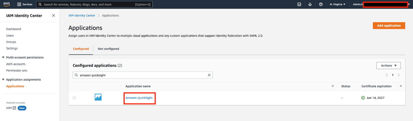
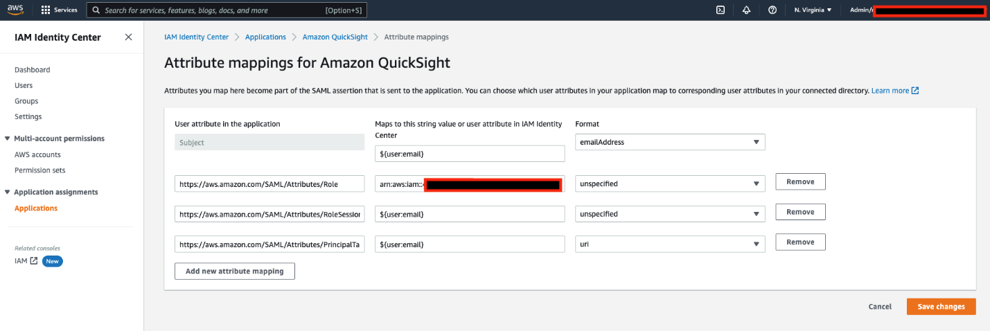
MSK Connect is a managed Kafka Connect service that allows you to deploy Kafka connectors into your environment with seamless integrations with AWS services like IAM, Amazon MSK, and Amazon CloudWatch.

In the following sections, we walk you through the steps to configure this solution:

  1. Create an IAM policy and role.
  2. Upload your data.
  3. Create a custom plugin.
  4. Create and deploy connectors.

Create an IAM policy and role for authentication

IAM helps users securely control access to AWS resources. In this step, we create an IAM policy and role that has two critical permissions:

A common mistake made when creating an IAM role and policy needed for common Kafka tasks (publishing to a topic, listing topics) is to assume that the AWS managed policy AmazonMSKFullAccess (arn:aws:iam::aws:policy/AmazonMSKFullAccess) will suffice for permissions.

The following is an example of a policy with both full Kafka and Amazon MSK access:

{
    "Version": "2012-10-17",
    "Statement": [
        {
            "Effect": "Allow",
            "Action": [
                "kafka-cluster:*",
                "kafka:*",
            ],
            "Resource": [
                "*"
            ]
        }
    ]
}

This policy supports the creation of the cluster within the AWS account infrastructure and grants access to the components that make up the cluster anatomy like Amazon Elastic Compute Cloud (Amazon EC2), Amazon Virtual Private Cloud (Amazon VPC), logs, and kafka:*. There is no managed policy for a Kafka administrator to have full access on the cluster itself.

After you create the KafkaAdminFullAccess policy, create a role and attach the policy to it. You need two entries on the role’s Trust relationships tab:

  • The first statement allows Kafka Connect to assume this role and connect to the cluster.
  • The second statement follows the pattern arn:aws:sts::(YOUR ACCOUNT NUMBER):assumed-role/(YOUR ROLE NAME)/(YOUR ACCOUNT NUMBER). Your account number should be the same account number where MSK Connect and the role are being created in. This role is the role you’re editing the trust entity on. In the following example code, I’m editing a role called MSKConnectExample in my account. This is so that when MSK Connect assumes the role, the assumed user can assume the role again to publish and consume records on the target cluster.

In the following example trust policy, provide your own account number and role name:

{
	"Version": "2012-10-17",
	"Statement": [
		{
			"Effect": "Allow",
			"Principal": {
				"Service": "kafkaconnect.amazonaws.com"
			},
			"Action": "sts:AssumeRole"
		},
		{
			"Effect": "Allow",
			"Principal": {
				"AWS": "arn:aws:sts::123456789101:assumed-role/MSKConnectExampleRole/123456789101"
			},
			"Action": "sts:AssumeRole"
		}
	]
}

Now we’re ready to deploy MirrorMaker 2.

Upload data

MSK Connect custom plugins accept a file or folder with a .jar or .zip ending. For this step, create a dummy folder or file and compress it. Then upload the .zip object to your Amazon Simple Storage Service (Amazon S3) bucket:

mkdir mm2 
zip mm2.zip mm2 
aws s3 cp mm2.zip s3://mytestbucket/

Because Kafka and subsequently Kafka Connect have MirrorMaker libraries built in, you don’t need to add additional JAR files for this functionality. MSK Connect has a prerequisite that a custom plugin needs to be present at connector creation, so we have to create an empty one just for reference. It doesn’t matter what the contents of the file are or what the folder contains, as long as there is an object in Amazon S3 that is accessible to MSK Connect, so MSK Connect has access to MM2 classes.

Create a custom plugin

On the Amazon MSK console, follow the steps to create a custom plugin from the .zip file. Enter the object’s Amazon S3 URI and for this post, and name the plugin Mirror-Maker-2.

custom plugin console

Create and deploy connectors

You need to deploy three connectors for a successful mirroring operation:

  • MirrorSourceConnector
  • MirrorHeartbeatConnector
  • MirrorCheckpointConnector

Complete the following steps for each connector:

  1. On the Amazon MSK console, choose Create connector.
  2. For Connector name, enter the name of your first connector.
    connector properties name
  3. Select the target MSK cluster that the data is mirrored to as a destination.
  4. Choose IAM as the authentication mechanism.
    select cluster
  5. Pass the config into the connector.
    connector config

Connector config files are JSON-formatted config maps for the Kafka Connect framework to use in passing configurations to the executable JAR. When using the MSK Connect console, we must convert the config file from a JSON config file to single-lined key=value (with no spaces) file.

You need to change some values within the configs for deployment, namely bootstrap.server, sasl.jaas.config and tasks.max. Note the placeholders in the following code for all three configs.

The following code is for MirrorHeartBeatConnector:

connector.class=org.apache.kafka.connect.mirror.MirrorHeartbeatConnector
source.cluster.alias=source
target.cluster.alias=target
clusters=source,target
source.cluster.bootstrap.servers=(SOURCE BOOTSTRAP SERVERS)
target.cluster.security.protocol=SASL_SSL
target.cluster.producer.security.protocol=SASL_SSL
target.cluster.consumer.security.protocol=SASL_SSL
target.cluster.sasl.mechanism=AWS_MSK_IAM
target.cluster.producer.sasl.mechanism=AWS_MSK_IAM
target.cluster.consumer.sasl.mechanism=AWS_MSK_IAM
target.cluster.sasl.jaas.config=software.amazon.msk.auth.iam.IAMLoginModule required awsRoleArn="arn:aws:iam::(Your Account Number):role/(Your IAM role):role/mck-role" awsDebugCreds=true;
target.cluster.producer.sasl.jaas.config=software.amazon.msk.auth.iam.IAMLoginModule required awsRoleArn="arn:aws:iam::(Your Account Number):role/(Your IAM role)" awsDebugCreds=true;
target.cluster.consumer.sasl.jaas.config=software.amazon.msk.auth.iam.IAMLoginModule required awsRoleArn="arn:aws:iam::(Your Account Number):role/(Your IAM role)" awsDebugCreds=true;
target.cluster.sasl.client.callback.handler.class=software.amazon.msk.auth.iam.IAMClientCallbackHandler
target.cluster.producer.sasl.client.callback.handler.class=software.amazon.msk.auth.iam.IAMClientCallbackHandler
target.cluster.consumer.sasl.client.callback.handler.class=software.amazon.msk.auth.iam.IAMClientCallbackHandler
source.cluster.security.protocol=SASL_SSL
source.cluster.producer.security.protocol=SASL_SSL
source.cluster.consumer.security.protocol=SASL_SSL
source.cluster.sasl.mechanism=AWS_MSK_IAM
source.cluster.producer.sasl.mechanism=AWS_MSK_IAM
source.cluster.consumer.sasl.mechanism=AWS_MSK_IAM
source.cluster.sasl.jaas.config=software.amazon.msk.auth.iam.IAMLoginModule required awsRoleArn="arn:aws:iam::(Your Account Number):role/(Your IAM role)" awsDebugCreds=true;
source.cluster.producer.sasl.jaas.config=software.amazon.msk.auth.iam.IAMLoginModule required awsRoleArn="arn:aws:iam::(Your Account Number):role/(Your IAM role)" awsDebugCreds=true;
source.cluster.consumer.sasl.jaas.config=software.amazon.msk.auth.iam.IAMLoginModule required awsRoleArn="arn:aws:iam::(Your Account Number):role/(Your IAM role)" awsDebugCreds=true;
source.cluster.sasl.client.callback.handler.class=software.amazon.msk.auth.iam.IAMClientCallbackHandler
source.cluster.producer.sasl.client.callback.handler.class=software.amazon.msk.auth.iam.IAMClientCallbackHandler
source.cluster.consumer.sasl.client.callback.handler.class=software.amazon.msk.auth.iam.IAMClientCallbackHandler
topics=.*
topics.exclude=.*[-.]internal, .*.replica, __.*, .*-config, .*-status, .*-offset
groups.exclude=console-consumer-.*, connect-.*, __.*
refresh.groups.enabled=true
refresh.groups.interval.seconds=60
emit.checkpoints.enabled=true
consumer.auto.offset.reset=earliest
producer.linger.ms=500
producer.retry.backoff.ms=1000
producer.max.block.ms=10000
replication.factor=3
tasks.max=1
key.converter=org.apache.kafka.connect.converters.ByteArrayConverter
value.converter=org.apache.kafka.connect.converters.ByteArrayConverter

The following code is for MirrorCheckpointConnector:

connector.class=org.apache.kafka.connect.mirror.MirrorCheckpointConnector
source.cluster.alias=source
target.cluster.alias=target
clusters=source,target
source.cluster.bootstrap.servers=(Source Bootstrap Servers)
target.cluster.bootstrap.servers=(Target Bootstrap Servers)
target.cluster.security.protocol=SASL_SSL
target.cluster.producer.security.protocol=SASL_SSL
target.cluster.consumer.security.protocol=SASL_SSL
target.cluster.sasl.mechanism=AWS_MSK_IAM
target.cluster.producer.sasl.mechanism=AWS_MSK_IAM
target.cluster.consumer.sasl.mechanism=AWS_MSK_IAM
target.cluster.sasl.jaas.config=software.amazon.msk.auth.iam.IAMLoginModule required awsRoleArn="arn:aws:iam::(Your Account Number):role/(Your IAM role)" awsDebugCreds=true;
target.cluster.producer.sasl.jaas.config=software.amazon.msk.auth.iam.IAMLoginModule required awsRoleArn="arn:aws:iam::(Your Account Number):role/(Your IAM role)" awsDebugCreds=true;
target.cluster.consumer.sasl.jaas.config=software.amazon.msk.auth.iam.IAMLoginModule required awsRoleArn="arn:aws:iam::(Your Account Number):role/(Your IAM role)" awsDebugCreds=true;
target.cluster.sasl.client.callback.handler.class=software.amazon.msk.auth.iam.IAMClientCallbackHandler
target.cluster.producer.sasl.client.callback.handler.class=software.amazon.msk.auth.iam.IAMClientCallbackHandler
target.cluster.consumer.sasl.client.callback.handler.class=software.amazon.msk.auth.iam.IAMClientCallbackHandler
source.cluster.security.protocol=SASL_SSL
source.cluster.producer.security.protocol=SASL_SSL
source.cluster.consumer.security.protocol=SASL_SSL
source.cluster.sasl.mechanism=AWS_MSK_IAM
source.cluster.producer.sasl.mechanism=AWS_MSK_IAM
source.cluster.consumer.sasl.mechanism=AWS_MSK_IAM
source.cluster.sasl.jaas.config=software.amazon.msk.auth.iam.IAMLoginModule required awsRoleArn="arn:aws:iam::(Your Account Number):role/(Your IAM role)" awsDebugCreds=true;
source.cluster.producer.sasl.jaas.config=software.amazon.msk.auth.iam.IAMLoginModule required awsRoleArn="arn:aws:iam::(Your Account Number):role/(Your IAM role)" awsDebugCreds=true;
source.cluster.consumer.sasl.jaas.config=software.amazon.msk.auth.iam.IAMLoginModule required awsRoleArn="arn:aws:iam::(Your Account Number):role/(Your IAM role)" awsDebugCreds=true;
source.cluster.sasl.client.callback.handler.class=software.amazon.msk.auth.iam.IAMClientCallbackHandler
source.cluster.producer.sasl.client.callback.handler.class=software.amazon.msk.auth.iam.IAMClientCallbackHandler
source.cluster.consumer.sasl.client.callback.handler.class=software.amazon.msk.auth.iam.IAMClientCallbackHandler
topics=.*
topics.exclude=.*[-.]internal, .*.replica, __.*, .*-config, .*-status, .*-offset
groups.exclude=console-consumer-.*, connect-.*, __.*
refresh.groups.enabled=true
refresh.groups.interval.seconds=60
emit.checkpoints.enabled=true
consumer.auto.offset.reset=earliest
producer.linger.ms=500
producer.retry.backoff.ms=1000
producer.max.block.ms=10000
replication.factor=3
tasks.max=1
key.converter=org.apache.kafka.connect.converters.ByteArrayConverter
value.converter=org.apache.kafka.connect.converters.ByteArrayConverter
sync.group.offsets.interval.seconds=5

The following code is for MirrorSourceConnector:

connector.class=org.apache.kafka.connect.mirror.MirrorSourceConnector
# See note below about the recommendations
tasks.max=(NUMBER OF TASKS)
clusters=source,target
source.cluster.alias=source
target.cluster.alias=target
source.cluster.bootstrap.servers=(SOURCE BOOTSTRAP-SERVER)
source.cluster.producer.sasl.client.callback.handler.class=software.amazon.msk.auth.iam.IAMClientCallbackHandler
source.cluster.producer.security.protocol=SASL_SSL
source.cluster.producer.sasl.mechanism=AWS_MSK_IAM
source.cluster.producer.sasl.jaas.config=software.amazon.msk.auth.iam.IAMLoginModule required awsRoleArn="arn:aws:iam:: (Your Account Number):role/(Your IAM role)" awsDebugCreds=true;
source.cluster.consumer.sasl.client.callback.handler.class=software.amazon.msk.auth.iam.IAMClientCallbackHandler
source.cluster.consumer.sasl.jaas.config=software.amazon.msk.auth.iam.IAMLoginModule required awsRoleArn="arn:aws:iam:: (Your Account Number):role/(Your IAM role)" awsDebugCreds=true;
source.cluster.consumer.security.protocol=SASL_SSL
source.cluster.consumer.sasl.mechanism=AWS_MSK_IAM
source.cluster.sasl.jaas.config=software.amazon.msk.auth.iam.IAMLoginModule required awsRoleArn="arn:aws:iam:: (Your Account Number):role/(Your IAM role)" awsDebugCreds=true;
source.cluster.sasl.mechanism=AWS_MSK_IAM
source.cluster.security.protocol=SASL_SSL
source.cluster.sasl.client.callback.handler.class=software.amazon.msk.auth.iam.IAMClientCallbackHandler
target.cluster.bootstrap.servers=(TARGET BOOTSTRAP-SERVER)
target.cluster.security.protocol=SASL_SSL
target.cluster.sasl.jaas.config=software.amazon.msk.auth.iam.IAMLoginModule required awsRoleArn="arn:aws:iam:: (Your Account Number):role/(Your IAM role)" awsDebugCreds=true;
target.cluster.producer.sasl.mechanism=AWS_MSK_IAM
target.cluster.producer.security.protocol=SASL_SSL
target.cluster.producer.sasl.jaas.config=software.amazon.msk.auth.iam.IAMLoginModule required awsRoleArn="arn:aws:iam:: (Your Account Number):role/(Your IAM role)" awsDebugCreds=true;
target.cluster.producer.sasl.client.callback.handler.class=software.amazon.msk.auth.iam.IAMClientCallbackHandler
target.cluster.consumer.security.protocol=SASL_SSL
target.cluster.consumer.sasl.mechanism=AWS_MSK_IAM
target.cluster.consumer.sasl.client.callback.handler.class=software.amazon.msk.auth.iam.IAMClientCallbackHandler
target.cluster.consumer.sasl.jaas.config=software.amazon.msk.auth.iam.IAMLoginModule required awsRoleArn="arn:aws:iam:: (Your Account Number):role/(Your IAM role)" awsDebugCreds=true;
target.cluster.sasl.mechanism=AWS_MSK_IAM
target.cluster.sasl.client.callback.handler.class=software.amazon.msk.auth.iam.IAMClientCallbackHandler
refresh.groups.enabled=true
refresh.groups.interval.seconds=60
refresh.topics.interval.seconds=60
topics.exclude=.*[-.]internal,.*.replica,__.*,.*-config,.*-status,.*-offset
emit.checkpoints.enabled=true
topics=.*
value.converter=org.apache.kafka.connect.converters.ByteArrayConverter
key.converter=org.apache.kafka.connect.converters.ByteArrayConverter
producer.max.block.ms=10000
producer.linger.ms=500
producer.retry.backoff.ms=1000
sync.topic.configs.enabled=true
sync.topic.configs.interval.seconds=60
refresh.topics.enabled=true
groups.exclude=console-consumer-.*,connect-.*,__.*
consumer.auto.offset.reset=earliest
replication.factor=3

A general guideline for the number of tasks for a MirrorSourceConnector is one task per up to 10 partitions to be mirrored. For example, if a Kafka cluster has 15 topics with 12 partitions each for a total partition count of 180 partitions, we deploy at least 18 tasks for mirroring the workload.

Exceeding the recommended number of tasks for the source connector may lead to offsets that aren’t translated (negative consumer group offsets). For more information about this issue and its workarounds, refer to MM2 may not sync partition offsets correctly.

  1. For the heartbeat and checkpoint connectors, use provisioned scale with one worker, because there is only one task running for each of them.
  2. For the source connector, we set the maximum number of workers to the value decided for the tasks.max property.
    Note that we use the defaults of the auto scaling threshold settings for now.
    worker properties
  3. Although it’s possible to pass custom worker configurations, let’s leave the default option selected.
    worker config
  4. In the Access permissions section, we use the IAM role that we created earlier that has a trust relationship with kafkaconnect.amazonaws.com and kafka-cluster:* permissions. Warning signs display above and below the drop-down menu. These are to remind you that IAM roles and attached policies is a common reason why connectors fail. If you never get any log output upon connector creation, that is a good indicator of an improperly configured IAM role or policy permission problem.
    connect iam role
    On the bottom of this page is a warning box telling us not to use the aptly named AWSServiceRoleForKafkaConnect role. This is an AWS managed service role that MSK Connect needs to perform critical, behind-the-scenes functions upon connector creation. For more information, refer to Using Service-Linked Roles for MSK Connect.
  5. Choose Next.
    Depending on the authorization mechanism chosen when aligning the connector with a specific cluster (we chose IAM), the options in the Security section are preset and unchangeable. If no authentication was chosen and your cluster allows plaintext communication, that option is available under Encryption – in transit.
  6. Choose Next to move to the next page.
    access and encryption
  7. Choose your preferred logging destination for MSK Connect logs. For this post, I select Deliver to Amazon CloudWatch Logs and choose the log group ARN for my MSK Connect logs.
  8. Choose Next.
    logs properties
  9. Review your connector settings and choose Create connector.

A message appears indicating either a successful start to the creation process or immediate failure. You can now navigate to the Log groups page on the CloudWatch console and wait for the log stream to appear.

The CloudWatch logs indicate when connectors are successful or have failed faster than on the Amazon MSK console. You can see a log stream in your chosen log group get created within a few minutes after you create your connector. If your log stream never appears, this is an indicator that there was a misconfiguration in your connector config or IAM role and it won’t work.

cloudwatch

Verify that the connector launched successfully

In this section, we walk through two confirmation steps to determine a successful launch.

Check the log stream

Open the log stream that your connector is writing to. In the log, you can check if the connector has successfully launched and is publishing data to the cluster. In the following screenshot, we can confirm data is being published.

cloudwatch logs

Mirror data

The second step is to create a producer to send data to the source cluster. We use the console producer and consumer that Kafka ships with. You can follow Step 1 from the Apache Kafka quickstart.

  1. On a client machine that can access Amazon MSK, download Kafka from https://kafka.apache.org/downloads and extract it:
    tar -xzf kafka_2.13-3.1.0.tgz
    cd kafka_2.13-3.1.0

  2. Download the latest stable JAR for IAM authentication from the repository. As of this writing, it is 1.1.3:
    cd libs/
    wget https://github.com/aws/aws-msk-iam-auth/releases/download/v1.1.3/aws-msk-iam-auth-1.1.3-all.jar

  3. Next, we need to create our client.properties file that defines our connection properties for the clients. For instructions, refer to Configure clients for IAM access control. Copy the following example of the client.properties file:
    security.protocol=SASL_SSL
    sasl.mechanism=AWS_MSK_IAM
    sasl.jaas.config=software.amazon.msk.auth.iam.IAMLoginModule required;
    sasl.client.callback.handler.class=software.amazon.msk.auth.iam.IAMClientCallbackHandler

    You can place this properties file anywhere on your machine. For ease of use and simple referencing, I place mine inside kafka_2.13-3.1.0/bin.
    After we create the client.properties file and place the JAR in the libs directory, we’re ready to create the topic for our replication test.

  4. From the bin folder, run the kafka-topics.sh script:
    ./kafka-topics.sh --bootstrap-server $bss --create --topic MirrorMakerTest --replication-factor 2 --partitions 1 --command-config client.properties

    The details of the command are as follows:
    –bootstrap-server – Your bootstrap server of the source cluster.
    –topic – The topic name you want to create.
    –create – The action for the script to perform.
    –replication-factor – The replication factor for the topic.
    –partitions – Total number of partitions to create for the topic.
    –command-config – Additional configurations needed for successful running. Here is where we pass in the client.properties file we created in the previous step.

  5. We can list all the topics to see that it was successfully created:
    ./kafka-topics.sh --bootstrap-server $bss --list --command-config client.properties

    When defining bootstrap servers, it’s recommended to use one broker from each Availability Zone. For example:

    export bss=broker1:9098,broker2:9098,broker3:9098

    Similar to the create topic command, the preceding step simply calls list to show all topics available on the cluster. We can run this same command on our target cluster to see if MirrorMaker has replicated the topic.
    With our topic created, let’s start the consumer. This consumer is consuming from the target cluster. When the topic is mirrored with the default replication policy, it will have a source. prefixed to it.

  6. For our topic, we consume from source.MirrorMakerTest as shown in the following code:
    ./kafka-console-consumer.sh --bootstrap-server $targetcluster --topic source.MirrorMakerTest --consumer.config client.properties

    The details of the code are as follows:
    –bootstrap-server – Your target MSK bootstrap servers
    –topic – The mirrored topic
    –consumer.config – Where we pass in our client.properties file again to instruct the client how to authenticate to the MSK cluster
    After this step is successful, it leaves a consumer running all the time on the console until we either close the client connection or close our terminal session. You won’t see any messages flowing yet because we haven’t started producing to the source topic on the source cluster.

  7. Open a new terminal window, leaving the consumer open, and start the producer:
    ./kafka-console-producer.sh --bootstrap-server $bss --topic MirrorMakerTest --producer.config client.properties

    The details of the code are as follows:
    –bootstrap-server – The source MSK bootstrap servers
    –topic – The topic we’re producing to
    –producer.config – The client.properties file indicating which IAM authentication properties to use

    After this is successful, the console returns >, which indicates that it’s ready to produce what we type. Let’s produce some messages, as shown in the following screenshot. After each message, press Enter to have the client produce to the topic.

    producer input

    Switching back to the consumer’s terminal window, you should see the same messages being replicated and now showing on your console’s output.

    consumer output

Clean up

We can close the client connections now by pressing Ctrl+C to close the connections or by simply closing the terminal windows.

We can delete the topics on both clusters by running the following code:

./kafka-topics.sh --bootstrap-server $bss --delete --topic MirrorMakerTest --command-config client.properties

Delete the source cluster topic first, then the target cluster topic.

Finally, we can delete the three connectors via the Amazon MSK console by selecting them from the list of connectors and choosing Delete.

Conclusion

In this post, we showed how to use MSK Connect for MM2 deployment with IAM authentication. We successfully deployed the Amazon MSK custom plugin, and created the MM2 connector along with the accompanying IAM role. Then we deployed the MM2 connector onto our MSK Connect instances and watched as data was replicated successfully between two MSK clusters.

Using MSK Connect to deploy MM2 eases the administrative and operational burden of Kafka Connect and MM2, because the service handles the underlying resources, enabling you to focus on the connectors and data. The solution removes the need to have a dedicated infrastructure of a Kafka Connect cluster hosted on Amazon services like Amazon Elastic Compute Cloud (Amazon EC2), AWS Fargate, or Amazon EKS. The solution also automatically scales the resources for you (if configured to do so), which eliminates the need for the administers to check if the resources are scaling to meet demand. Additionally, using the Amazon managed service MSK Connect allows for easier compliance and security adherence for Kafka teams.

If you have any feedback or questions, please leave a comment.


About the Authors

tannerTanner Pratt is a Practice Manager at Amazon Web Services. Tanner is leading a team of consultants focusing on Amazon streaming services like Managed Streaming for Apache Kafka, Kinesis Data Streams/Firehose and Kinesis Data Analytics.
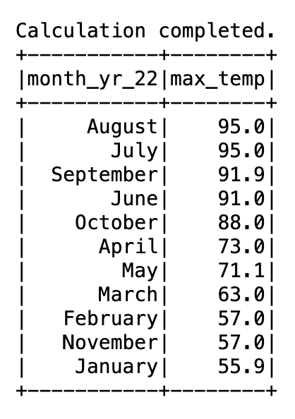
edberezEd Berezitsky is a Senior Data Architect at Amazon Web Services.Ed helps customers design and implement solutions using streaming technologies, and specializes on Amazon MSK and Apache Kafka.

Simplify semi-structured nested JSON data analysis with AWS Glue DataBrew and Amazon QuickSight

Post Syndicated from Sriharsh Adari original https://aws.amazon.com/blogs/big-data/simplify-semi-structured-nested-json-data-analysis-with-aws-glue-databrew-and-amazon-quicksight/

As the industry grows with more data volume, big data analytics is becoming a common requirement in data analytics and machine learning (ML) use cases. Data comes from many different sources in structured, semi-structured, and unstructured formats. For semi-structured data, one of the most common lightweight file formats is JSON. However, due to the complex nature of data, JSON often includes nested key-value structures. Analysts may want a simpler graphical user interface to conduct data analysis and profiling.


To support these requirements, AWS Glue DataBrew offers an easy visual data preparation tool with over 350 pre-built transformations. You can use DataBrew to analyze complex nested JSON files that would otherwise require days or weeks writing hand-coded transformations. You can then use Amazon QuickSight for data analysis and visualization.

In this post, we demonstrate how to configure DataBrew to work with nested JSON objects and use QuickSight for data visualization.

Solution overview

To implement our solution, we create a DataBrew project and DataBrew job for unnesting data. We profile the unested data in DataBrew and analyze data in QuickSight. The following diagram illustrates the architecture of this solution.

Prerequisites

Before you get started, make sure you have the following prerequisites:

Prepare the data

To illustrate the DataBrew functionality to support data analysis for nested JSON files, we use a publicly available sample customer order details nested JSON dataset.

Complete the following steps to prepare your data:

  1. Sign in to the AWS Management Console.
  2. Browse to the publicly available datasets on the Amazon S3 console.
  3. Select the first dataset (customer_1.json) and choose Download to save the files on your local machine.
  4. Repeat this step to download all three JSON files.

    You can view the sample data from your local machine using any text editor, as shown in the following screenshot.
  5. Create input and output S3 buckets with subfolders nestedjson and outputjson to capture data.
  6. Choose Upload and upload the three JSON files to the nestedjson folder.

Create a DataBrew project

To create your Amazon S3 connection, complete the following steps:

  1. On the DataBrew console, choose Projects in the navigation pane.
  2. Choose Create project.
  3. For Project name, enter Glue-DataBew-NestedJSON-Blog.
  4. Select New dataset.
  5. For Dataset name, enter Glue-DataBew-NestedJSON-Dataset.
  6. For Enter your source from S3, enter the path to the nestedjson folder.
  7. Choose Select the entire folder to select all the files.
  8. Under Additional configurations, select JSON as the file type, then select JSON document.
  9. In the Permissions section, choose Choose existing IAM role if you have one available, or choose Create new IAM role.
  10. Choose Create project.
  11. Skip the preview steps and wait for the project to be ready.
    As shown in the following screenshot, the three JSON files were uploaded to the S3 bucket, so three rows of customer order details are loaded.
    The orders column contains nested files. We can use DataBrew to unnest or nest transform to flatten the columns and rows.
  12. Choose the menu icon (three dots) and choose Nest-unnest.
  13. Depending on the nesting, either choose Unnest to columns or Unnest to rows. In this blog post, we choose Unnest to columns to flatten example JSON file.

    Repeat this step until you get a flattened json for all the nested json data and this will create the AWS Glue Databrew recipe as shown below.
  14. Choose Apply.

    DataBrew automatically creates the required recipe steps with updated column values.
  15. Choose Create job.
  16. For Job name, enter Glue-DataBew-NestedJSON-job.
  17. For S3 location, enter the path to the outputjson folder.
  18. In the Permissions section, for Role name, choose the role you created earlier.
  19. Choose Create and run job.

On the Jobs page, you can choose the job to view its run history, details, and data lineage.

Profile the metadata with DataBrew

After you have a flattened file in the S3 output bucket, you can use DataBrew to carry out the data analysis and profiling for the flattened file. Complete the following steps:

  1. On the Datasets page, choose Connect new datasets.
  2. Provide your dataset details and choose Create dataset.
  3. Choose the newly added data source, then choose the Data profile overview tab.
  4. Enter the name of the job and the S3 path to save the output.
  5. Choose Create and run job.

The job takes around two minutes to complete and display all the updated information. You can explore the data further on the Data profile overview and Column statistics tabs.

Visualize the data in QuickSight

After you have the output file generated by DataBrew in the S3 output bucket, you can use QuickSight to query the JSON data. QuickSight is a scalable, serverless, embeddable, ML-powered business intelligence (BI) service built for the cloud. QuickSight lets you easily create and publish interactive BI dashboards that include ML-powered insights. QuickSight dashboards can be accessed from any device, and seamlessly embedded into your applications, portals, and websites.

Launch QuickSight

On the console, enter quicksight into the search bar and choose QuickSight.

You’re presented with the QuickSight welcome page. If you haven’t signed up for QuickSight, you may have to complete the signup wizard. For more information, refer to Signing up for an Amazon QuickSight subscription.

After you have signed up, QuickSight presents a “Welcome wizard.” You can view the short tutorial, or you can close it.

Grant Amazon S3 access

To grant Amazon S3 access, complete the following steps:

  1. On the QuickSight console, choose your user name, choose Manage QuickSight, then choose Security & permissions.
  2. Choose Add or remove.
  3. Locate Amazon S3 in the list. Choose one of the following:
    1. If the check box is clear, select Amazon S3.
    2. If the check box is already selected, choose Details, then choose Select S3 buckets.
  4. Choose the buckets that you want to access from QuickSight, then choose Select.
  5. Choose Update.
  6. If you changed your Region during the first step of this process, change it back to the Region that you want to use.

Create a dataset

Now that you have QuickSight up and running, you can create your dataset. Complete the following steps:

  1. On the QuickSight console, choose Datasets in the navigation pane.
  2. Choose New dataset.

    QuickSight supports several data sources. For a complete list, refer to Supported data sources.
  3. For your data source, choose S3.

    The S3 import requires a data source name and a manifest file.
  4. On your machine, use a text editor to create a manifest file called BlogGlueDataBrew.manifest using the following structure (provide the name of the your output bucket):
    {
        "fileLocations": [
            {
                "URIPrefixes": [
                "https://s3.amazonaws.com/ s3://<output bucket>/outputjson/"
                ]
            }
        ],
        "globalUploadSettings": {
            "format": "CSV",
            "delimiter": ","
        }
    }

    The manifest file points to the folder that you created earlier as part of your DataBrew project. For more information, refer to Supported formats for Amazon S3 manifest files.

  5. Select Upload and navigate to the manifest file to upload it.
  6. Choose Connect to upload data into SPICE, which is an in-memory database built into QuickSight to achieve fast performance.
  7. Choose Visualize.

You can now create visuals by adding different fields.

To learn more about authoring dashboards in QuickSight, check out the QuickSight Author Workshop.

Clean up

Complete the following steps to avoid incurring future charges:

  1. On the DataBrew console, choose Projects in the navigation pane.
  2. Select the project you created and on the Actions menu, choose Delete.
  3. Choose Jobs in the navigation pane.
  4. Select the job you created and on the Actions menu, choose Delete.
  5. Choose Recipes in the navigation pane.
  6. Select the recipe you created and on the Actions menu, choose Delete.
  7. On the QuickSight dashboard, choose your user name on the application bar, then choose Manage QuickSight.
  8. Choose Account settings, then choose Delete account.
  9. Choose Delete account.
  10. Enter confirm and choose Delete account.

Conclusion

This post walked you through the steps to configure DataBrew to work with nested JSON objects and use QuickSight for data visualization. We used Glue DataBrew to unnest our JSON file and profile the data, and then used QuickSight to create dashboards and visualizations for further analysis.

You can use this solution for your own use cases when you need to unnest complex semi-structured JSON files without writing code. If you have comments or feedback, please leave them in the comments section.


About the authors

Sriharsh Adari is a Senior Solutions Architect at Amazon Web Services (AWS), where he helps customers work backwards from business outcomes to develop innovative solutions on AWS. Over the years, he has helped multiple customers on data platform transformations across industry verticals. His core area of expertise include Technology Strategy, Data Analytics, and Data Science. In his spare time, he enjoys playing sports, binge-watching TV shows, and playing Tabla.

Rahul Sonawane is a Principal Analytics Solutions Architect at AWS with AI/ML and Analytics as his area of specialty.

Amogh Gaikwad is a Solutions Developer at Amazon Web Services. He helps global customers build and deploy AI/ML solutions. His work is mainly focused on computer vision, and NLP uses-cases and helping customers optimize their AI/ML workloads for sustainability. Amogh has received his master’s in Computer Science specializing in Machine Learning.