Post Syndicated from Yonatan Dolan original https://aws.amazon.com/blogs/big-data/orca-securitys-journey-to-a-petabyte-scale-data-lake-with-apache-iceberg-and-aws-analytics/
This post is co-written with Eliad Gat and Oded Lifshiz from Orca Security.
With data becoming the driving force behind many industries today, having a modern data architecture is pivotal for organizations to be successful. One key component that plays a central role in modern data architectures is the data lake, which allows organizations to store and analyze large amounts of data in a cost-effective manner and run advanced analytics and machine learning (ML) at scale.
Orca Security is an industry-leading Cloud Security Platform that identifies, prioritizes, and remediates security risks and compliance issues across your AWS Cloud estate. Orca connects to your environment in minutes with patented SideScanning technology to provide complete coverage across vulnerabilities, malware, misconfigurations, lateral movement risk, weak and leaked passwords, overly permissive identities, and more.
The Orca Platform is powered by a state-of-the-art anomaly detection system that uses cutting-edge ML algorithms and big data capabilities to detect potential security threats and alert customers in real time, ensuring maximum security for their cloud environment. At the core of Orca’s anomaly detection system is its transactional data lake, which enables the company’s data scientists, analysts, data engineers, and ML specialists to extract valuable insights from vast amounts of data and deliver innovative cloud security solutions to its customers.
In this post, we describe Orca’s journey building a transactional data lake using Amazon Simple Storage Service (Amazon S3), Apache Iceberg, and AWS Analytics. We explore why Orca chose to build a transactional data lake and examine the key considerations that guided the selection of Apache Iceberg as the preferred table format.
In addition, we describe the Orca Platform architecture and the technologies used. Lastly, we discuss the challenges encountered throughout the project, present the solutions used to address them, and share valuable lessons learned.
Why did Orca build a data lake?
Prior to the creation of the data lake, Orca’s data was distributed among various data silos, each owned by a different team with its own data pipelines and technology stack. This setup led to several issues, including scaling difficulties as the data size grew, maintaining data quality, ensuring consistent and reliable data access, high costs associated with storage and processing, and difficulties supporting streaming use cases. Moreover, running advanced analytics and ML on disparate data sources proved challenging. To overcome these issues, Orca decided to build a data lake.
A data lake is a centralized data repository that enables organizations to store and manage large volumes of structured and unstructured data, eliminating data silos and facilitating advanced analytics and ML on the entire data. By decoupling storage and compute, data lakes promote cost-effective storage and processing of big data.
Why did Orca choose Apache Iceberg?
Orca considered several table formats that have evolved in recent years to support its transactional data lake. Amongst the options, Apache Iceberg stood out as the ideal choice because it met all of Orca’s requirements.
First, Orca sought a transactional table format that ensures data consistency and fault tolerance. Apache Iceberg’s transactional and ACID guarantees, which allow concurrent read and write operations while ensuring data consistency and simplified fault handling, fulfill this requirement. Furthermore, Apache Iceberg’s support for time travel and rollback capabilities makes it highly suitable for addressing data quality issues by reverting to a previous state in a consistent manner.
Second, a key requirement was to adopt an open table format that integrates with various processing engines. This was to avoid vendor lock-in and allow teams to choose the processing engine that best suits their needs. Apache Iceberg’s engine-agnostic and open design meets this requirement by supporting all popular processing engines, including Apache Spark, Amazon Athena, Apache Flink, Trino, Presto, and more.
In addition, given the substantial data volumes handled by the system, an efficient table format was required that can support querying petabytes of data very fast. Apache Iceberg’s architecture addresses this need by efficiently filtering and reducing scanned data, resulting in accelerated query times.
An additional requirement was to allow seamless schema changes without impacting end-users. Apache Iceberg’s range of features, including schema evolution, hidden partitions, and partition evolution, addresses this requirement.
Lastly, it was important for Orca to choose a table format that is widely adopted. Apache Iceberg’s growing and active community aligned with the requirement for a popular and community-backed table format.
Solution overview
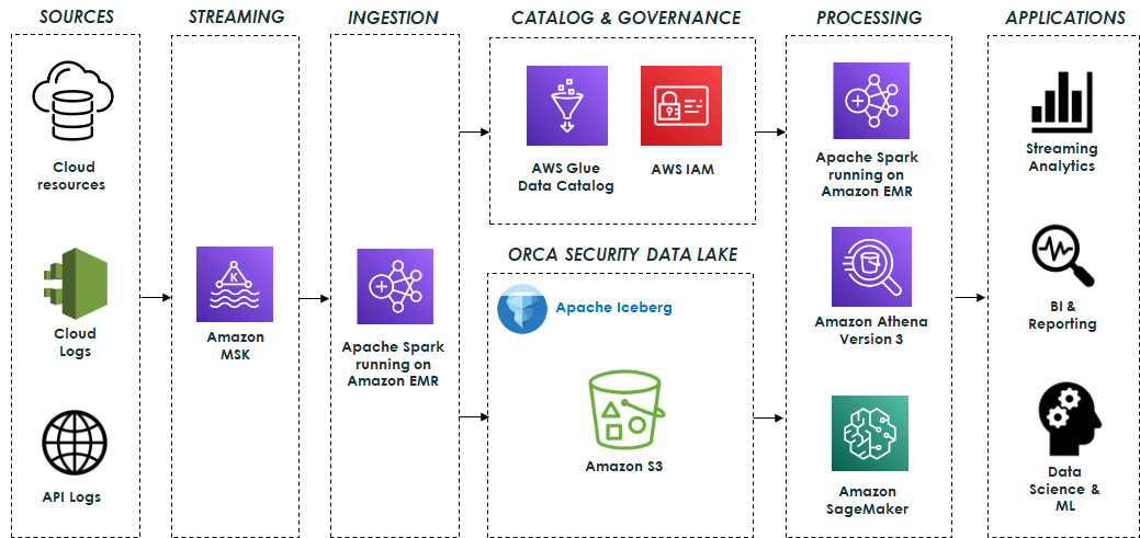
Orca’s data lake is based on open-source technologies that seamlessly integrate with Apache Iceberg. The system ingests data from various sources such as cloud resources, cloud activity logs, and API access logs, and processes billions of messages, resulting in terabytes of data daily. This data is sent to Apache Kafka, which is hosted on Amazon Managed Streaming for Apache Kafka (Amazon MSK). It is then processed using Apache Spark Structured Streaming running on Amazon EMR and stored in the data lake. Amazon EMR streamlines the process of loading all required Iceberg packages and dependencies, ensuring that the data is stored in Apache Iceberg format and ready for consumption as quickly as possible.
The data lake is built on top of Amazon S3 using Apache Iceberg table format with Apache Parquet as the underlying file format. In addition, the AWS Glue Data Catalog enables data discovery, and AWS Identity and Access Management (IAM) enforces secure access controls for the lake and its operations.
The data lake serves as the foundation for a variety of capabilities that are supported by different engines.
Data pipelines built on Apache Spark and Athena SQL analyze and process the data stored in the data lake. These data pipelines generate valuable insights and curated data that are stored in Apache Iceberg tables for downstream usage. This data is then used by various applications for streaming analytics, business intelligence, and reporting.
Amazon SageMaker is used to build, train, and deploy a range of ML models. Specifically, the system uses Amazon SageMaker Processing jobs to process the data stored in the data lake, employing the AWS SDK for Pandas (previously known as AWS Wrangler) for various data transformation operations, including cleaning, normalization, and feature engineering. This ensures that the data is suitable for training purposes. Additionally, SageMaker training jobs are employed for training the models. After the models are trained, they are deployed and used to identify anomalies and alert customers in real time to potential security threats. The following diagram illustrates the solution architecture.

Challenges and lessons learned
Orca faced several challenges while building its petabyte-scale data lake, including:
- Determining optimal table partitioning
- Optimizing EMR streaming ingestion for high throughput
- Taming the small files problem for fast reads
- Maximizing performance with Athena version 3
- Maintaining Apache Iceberg tables
- Managing data retention
- Monitoring the data lake infrastructure and operations
- Mitigating data quality issues
In this section, we describe each of these challenges and the solutions implemented to address them.
Determining optimal table partitioning
Determining optimal partitioning for each table is very important in order to optimize query performance and minimize the impact on teams querying the tables when partitioning changes. Apache Iceberg’s hidden partitions combined with partition transformations proved to be valuable in achieving this goal because it allowed for transparent changes to partitioning without impacting end-users. Additionally, partition evolution enables experimentation with various partitioning strategies to optimize cost and performance without requiring a rewrite of the table’s data every time.
For example, with these features, Orca was able to easily change several of its table partitioning from DAY to HOUR with no impact on user queries. Without this native Iceberg capability, they would have needed to coordinate the new schema with all the teams that query the tables and rewrite the entire data, which would have been a costly, time-consuming, and error-prone process.
Optimizing EMR streaming ingestion for high throughput
As mentioned previously, the system ingests billions of messages daily, resulting in terabytes of data processed and stored each day. Therefore, optimizing the EMR clusters for this type of load while maintaining high throughput and low costs has been an ongoing challenge. Orca addressed this in several ways.
First, Orca chose to use instance fleets with its EMR clusters because they allow optimized resource allocation by combining different instance types and sizes. Instance fleets improve resilience by allowing multiple Availability Zones to be configured. As a result, the cluster will launch in an Availability Zone with all the required instance types, preventing capacity limitations. Additionally, instance fleets can use both Amazon Elastic Compute Cloud (Amazon EC2) On-Demand and Spot instances, resulting in cost savings.
The process of sizing the cluster for high throughput and lower costs involved adjusting the number of core and task nodes, selecting suitable instance types, and fine-tuning CPU and memory configurations. Ultimately, Orca was able to find an optimal configuration consisting of on-demand core nodes and spot task nodes of varying sizes, which provided high throughput but also ensured compliance with SLAs.
Orca also found that using different Kafka Spark Structured Streaming properties, such as minOffsetsPerTrigger, maxOffsetsPerTrigger, and minPartitions, provided higher throughput and better control of the load. Using minPartitions, which enables better parallelism and distribution across a larger number of tasks, was particularly useful for consuming high lags quickly.
Lastly, when dealing with a high data ingestion rate, Amazon S3 may throttle the requests and return 503 errors. To address this scenario, Iceberg offers a table property called write.object-storage.enabled, which incorporates a hash prefix into the stored S3 object path. This approach effectively mitigates throttling problems.
Taming the small files problem for fast reads
A common challenge often encountered when ingesting streaming data into the data lake is the creation of many small files. This can have a negative impact on read performance when querying the data with Athena or Apache Spark. Having a high number of files leads to longer query planning and runtimes due to the need to process and read each file, resulting in overhead for file system operations and network communication. Additionally, this can result in higher costs due to the large number of S3 PUT and GET requests required.
To address this challenge, Apache Spark Structured Streaming provides the trigger mechanism, which can be used to tune the rate at which data is committed to Apache Iceberg tables. The commit rate has a direct impact on the number of files being produced. For instance, a higher commit rate, corresponding to a shorter time interval, results in lots of data files being produced.
In certain cases, launching the Spark cluster on an hourly basis and configuring the trigger to AvailableNow facilitated the processing of larger data batches and reduced the number of small files created. Although this approach led to cost savings, it did involve a trade-off of reduced data freshness. However, this trade-off was deemed acceptable for specific use cases.
In addition, to address preexisting small files within the data lake, Apache Iceberg offers a data files compaction operation that combines these smaller files into larger ones. Running this operation on a schedule is highly recommended to optimize the number and size of the files. Compaction also proves valuable in handling late-arriving data and enables the integration of this data into consolidated files.
Maximizing performance with Athena version 3
Orca was an early adopter of Athena version 3, Amazon’s implementation of the Trino query engine, which provides extensive support for Apache Iceberg. Whenever possible, Orca preferred using Athena over Apache Spark for data processing. This preference was driven by the simplicity and serverless architecture of Athena, which led to reduced costs and easier usage, unlike Spark, which typically required provisioning and managing a dedicated cluster at higher costs.
In addition, Orca used Athena as part of its model training and as the primary engine for ad hoc exploratory queries conducted by data scientists, business analysts, and engineers. However, for maintaining Iceberg tables and updating table properties, Apache Spark remained the more scalable and feature-rich option.
Maintaining Apache Iceberg tables
Ensuring optimal query performance and minimizing storage overhead became a significant challenge as the data lake grew to a petabyte scale. To address this challenge, Apache Iceberg offers several maintenance procedures, such as the following:
- Data files compaction – This operation, as mentioned earlier, involves combining smaller files into larger ones and reorganizing the data within them. This operation not only reduces the number of files but also enables data sorting based on different columns or clustering similar data using z-ordering. Using Apache Iceberg’s compaction results in significant performance improvements, especially for large tables, making a noticeable difference in query performance between compacted and uncompacted data.
- Expiring old snapshots – This operation provides a way to remove outdated snapshots and their associated data files, enabling Orca to maintain low storage costs.
Running these maintenance procedures efficiently and cost-effectively using Apache Spark, particularly the compaction operation, which operates on terabytes of data daily, requires careful consideration. This entails appropriately sizing the Spark cluster running on EMR and adjusting various settings such as CPU and memory.
In addition, using Apache Iceberg’s metadata tables proved to be very helpful in identifying issues related to the physical layout of Iceberg’s tables, which can directly impact query performance. Metadata tables offer insights into the physical data storage layout of the tables and offer the convenience of querying them with Athena version 3. By accessing the metadata tables, crucial information about tables’ data files, manifests, history, partitions, snapshots, and more can be obtained, which aids in understanding and optimizing the table’s data layout.
For instance, the following queries can uncover valuable information about the underlying data:
- The number of files and their average size per partition:
>SELECT partition, file_count, (total_size / file_count) AS avg_file_size FROM "db"."table$partitions"
- The number of data files pointed to by each manifest:
SELECT path, added_data_files_count + existing_data_files_count AS number_of_data_files FROM "db"."table$manifests"
- Information about the data files:
SELECT file_path, file_size_in_bytes FROM "db"."table$files"
- Information related to data completeness:
SELECT record_count, partition FROM "db"."table$partitions"
Managing data retention
Effective management of data retention in a petabyte-scale data lake is crucial to ensure low storage costs as well as to comply with GDPR. However, implementing such a process can be challenging when dealing with Iceberg data stored in S3 buckets, because deleting files based on simple S3 lifecycle policies could potentially cause table corruption. This is because Iceberg’s data files are referenced in manifest files, so any changes to data files must also be reflected in the manifests.
To address this challenge, certain considerations must be taken into account while handling data retention properly. Apache Iceberg provides two modes for handling deletes, namely copy-on-write (CoW), and merge-on-read (MoR). In CoW mode, Iceberg rewrites data files at the time of deletion and creates new data files, whereas in MoR mode, instead of rewriting the data files, a delete file is written that lists the position of deleted records in files. These files are then reconciled with the remaining data during read time.
In favor of faster read times, CoW mode is preferable and when used in conjunction with the expiring old snapshots operation, it allows for the hard deletion of data files that have exceeded the set retention period.
In addition, by storing the data sorted based on the field that will be utilized for deletion (for example, organizationID), it’s possible to reduce the number of files that require rewriting. This optimization significantly enhances the efficiency of the deletion process, resulting in improved deletion times.
Monitoring the data lake infrastructure and operations
Managing a data lake infrastructure is challenging due to the various components it encompasses, including those responsible for data ingestion, storage, processing, and querying.
Effective monitoring of all these components involves tracking resource utilization, data ingestion rates, query runtimes, and various other performance-related metrics, and is essential for maintaining optimal performance and detecting issues as soon as possible.
Monitoring Amazon EMR was crucial because it played a vital role in the system for data ingestion, processing, and maintenance. Orca monitored the cluster status and resource usage of Amazon EMR by utilizing the available metrics through Amazon CloudWatch. Furthermore, it used JMX Exporter and Prometheus to scrape specific Apache Spark metrics and create custom metrics to further improve the pipelines’ observability.
Another challenge emerged when attempting to further monitor the ingestion progress through Kafka lag. Although Kafka lag tracking is the standard method for monitoring ingestion progress, it posed a challenge because Spark Structured Streaming manages its offsets internally and doesn’t commit them back to Kafka. To overcome this, Orca utilized the progress of the Spark Structured Streaming Query Listener (StreamingQueryListener) to monitor the processed offsets, which were then committed to a dedicated Kafka consumer group for lag monitoring.
In addition, to ensure optimal query performance and identify potential performance issues, it was essential to monitor Athena queries. Orca addressed this by using key metrics from Athena and the AWS SDK for Pandas, specifically TotalExecutionTime and ProcessedBytes. These metrics helped identify any degradation in query performance and keep track of costs, which were based on the size of the data scanned.
Mitigating data quality issues
Apache Iceberg’s capabilities and overall architecture played a key role in mitigating data quality challenges.
One of the ways Apache Iceberg addresses these challenges is through its schema evolution capability, which enables users to modify or add columns to a table’s schema without rewriting the entire data. This feature prevents data quality issues that may arise due to schema changes, because the table’s schema is managed as part of the manifest files, ensuring safe changes.
Furthermore, Apache Iceberg’s time travel feature provides the ability to review a table’s history and roll back to a previous snapshot. This functionality has proven to be extremely useful in identifying potential data quality issues and swiftly resolving them by reverting to a previous state with known data integrity.
These robust capabilities ensure that data within the data lake remains accurate, consistent, and reliable.
Conclusion
Data lakes are an essential part of a modern data architecture, and now it’s easier than ever to create a robust, transactional, cost-effective, and high-performant data lake by using Apache Iceberg, Amazon S3, and AWS Analytics services such as Amazon EMR and Athena.
Since building the data lake, Orca has observed significant improvements. The data lake infrastructure has allowed Orca’s platform to have seamless scalability while reducing the cost of running its data pipelines by over 50% utilizing Amazon EMR. Additionally, query costs were reduced by more than 50% using the efficient querying capabilities of Apache Iceberg and Athena version 3.
Most importantly, the data lake has made a profound impact on Orca’s platform and continues to play a key role in its success, supporting new use cases such as change data capture (CDC) and others, and enabling the development of cutting-edge cloud security solutions.
If Orca’s journey has sparked your interest and you are considering implementing a similar solution in your organization, here are some strategic steps to consider:
- Start by thoroughly understanding your organization’s data needs and how this solution can address them.
- Reach out to experts, who can provide you with guidance based on their own experiences. Consider engaging in seminars, workshops, or online forums that discuss these technologies. The following resources are recommended for getting started:
- An important part of this journey would be to implement a proof of concept. This hands-on experience will provide valuable insights into the complexities of a transactional data lake.
Embarking on a journey to a transactional data lake using Amazon S3, Apache Iceberg, and AWS Analytics can vastly improve your organization’s data infrastructure, enabling advanced analytics and machine learning, and unlocking insights that drive innovation.
About the Authors
 Eliad Gat is a Big Data & AI/ML Architect at Orca Security. He has over 15 years of experience designing and building large-scale cloud-native distributed systems, specializing in big data, analytics, AI, and machine learning.
 Oded Lifshiz is a Principal Software Engineer at Orca Security. He enjoys combining his passion for delivering innovative, data-driven solutions with his expertise in designing and building large-scale machine learning pipelines.
 Yonatan Dolan is a Principal Analytics Specialist at Amazon Web Services. He is located in Israel and helps customers harness AWS analytical services to leverage data, gain insights, and derive value. Yonatan also leads the Apache Iceberg Israel community.
Carlos Rodrigues is a Big Data Specialist Solutions Architect at Amazon Web Services. He helps customers worldwide build transactional data lakes on AWS using open table formats like Apache Hudi and Apache Iceberg.
 Sofia Zilberman is a Sr. Analytics Specialist Solutions Architect at Amazon Web Services. She has a track record of 15 years of creating large-scale, distributed processing systems. She remains passionate about big data technologies and architecture trends, and is constantly on the lookout for functional and technological innovations.


 Ali Alemi is a Streaming Specialist Solutions Architect at AWS. Ali advises AWS customers with architectural best practices and helps them design real-time analytics data systems that are reliable, secure, efficient, and cost-effective. He works backward from customer’s use cases and designs data solutions to solve their business problems. Prior to joining AWS, Ali supported several public sector customers and AWS consulting partners in their application modernization journey and migration to the Cloud.


 Amar is a Senior Solutions Architect at Amazon AWS in the UK. He works across power, utilities, manufacturing and automotive customers on strategic implementations, specializing in using AWS Streaming and advanced data analytics solutions, to drive optimal business outcomes.


 M Mehrtens has been working in distributed systems engineering throughout their career, working as a Software Engineer, Architect, and Data Engineer. In the past, M has supported and built systems to process terrabytes of streaming data at low latency, run enterprise Machine Learning pipelines, and created systems to share data across teams seamlessly with varying data toolsets and software stacks. At AWS, they are a Sr. Solutions Architect supporting US Federal Financial customers.
 Sindhu Achuthan is a Sr. Solutions Architect with Federal Financials at AWS. She works with customers to provide architectural guidance on analytics solutions using AWS Glue, Amazon EMR, Amazon Kinesis, and other services. Outside of work, she loves DIYs, to go on long trails, and yoga.


 Florian Mair is a Senior Solutions Architect and data streaming expert at AWS. He is a technologist that helps customers in Germany succeed and innovate by solving business challenges using AWS Cloud services. Besides working as a Solutions Architect, Florian is a passionate mountaineer, and has climbed some of the highest mountains across Europe.
 Benjamin Meyer is a Senior Solutions Architect at AWS, focused on Games businesses in Germany to solve business challenges by using AWS Cloud services. Benjamin has been an avid technologist for 7 years, and when he’s not helping customers, he can be found developing mobile apps, building electronics, or tending to his cacti.


 available.


 Rahul Nammireddy is a Senior Solutions Architect at AWS, focusses on guiding digital native customers through their cloud native transformation. With a passion for AI/ML technologies, he works with customers in industries such as retail and telecom, helping them innovate at a rapid pace. Throughout his 23+ years career, Rahul has held key technical leadership roles in a diverse range of companies, from startups to publicly listed organizations, showcasing his expertise as a builder and driving innovation. In his spare time, he enjoys watching football and playing cricket.
 Todd McGrath is a data streaming specialist at Amazon Web Services where he advises customers on their streaming strategies, integration, architecture, and solutions. On the personal side, he enjoys watching and supporting his 3 teenagers in their preferred activities as well as following his own pursuits such as fishing, pickleball, ice hockey, and happy hour with friends and family on pontoon boats. Connect with him on
  RamC Venkatasamy is a Solutions Architect based in Bloomington, Illinois. He helps AWS Strategic customers transform their businesses in the cloud. With a fervent enthusiasm for Serverless, Event-Driven Architecture and GenAI.
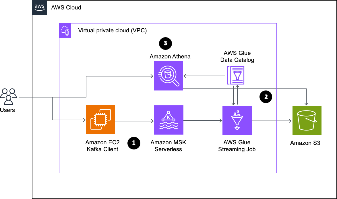


 Shubham Purwar is a Cloud Engineer (ETL) at AWS Bengaluru specialized in AWS Glue and Amazon Athena. He is passionate about helping customers solve issues related to their ETL workload and implement scalable data processing and analytics pipelines on AWS. In his free time, Shubham loves to spend time with his family and travel around the world.
 Nitin Kumar is a Cloud Engineer (ETL) at AWS with a specialization in AWS Glue. He is dedicated to assisting customers in resolving issues related to their ETL workloads and creating scalable data processing and analytics pipelines on AWS.
 Philipp Klose is a Global Solutions Architect at AWS based in Munich. He works with enterprise FSI customers and helps them solve business problems by architecting serverless platforms. In this free time, Philipp spends time with his family and enjoys every geek hobby possible.
 Daniel Wessendorf is a Global Solutions Architect at AWS based in Munich. He works with enterprise FSI customers and is primarily specialized in machine learning and data architectures. In his free time, he enjoys swimming, hiking, skiing, and spending quality time with his family.
 Marvin Gersho is a Senior Solutions Architect at AWS based in New York City. He works with a wide range of startup customers. He previously worked for many years in engineering leadership and hands-on application development, and now focuses on helping customers architect secure and scalable workloads on AWS with a minimum of operational overhead. In his free time, Marvin enjoys cycling and strategy board games.
 Nathan Lichtenstein is a Senior Solutions Architect at AWS based in New York City. Primarily working with startups, he ensures his customers build smart on AWS, delivering creative solutions to their complex technical challenges. Nathan has worked in cloud and network architecture in the media, financial services, and retail spaces. Outside of work, he can often be found at a Broadway theater.
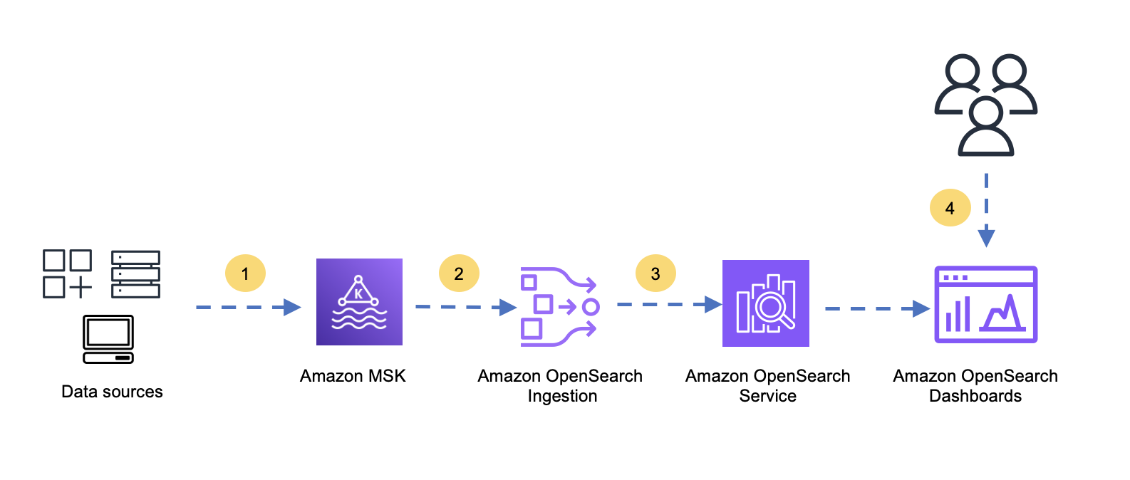

 Muthu Pitchaimani is a Search Specialist with Amazon OpenSearch Service. He builds large-scale search applications and solutions. Muthu is interested in the topics of networking and security, and is based out of Austin, Texas.
 Arjun Nambiar is a Product Manager with Amazon OpenSearch Service. He focusses on ingestion technologies that enable ingesting data from a wide variety of sources into Amazon OpenSearch Service at scale. Arjun is interested in large scale distributed systems and cloud-native technologies and is based out of Seattle, Washington.
 Raj Sharma is a Sr. SDM with Amazon OpenSearch Service. He builds large-scale distributed applications and solutions. Raj is interested in the topics of Analytics, databases, networking and security, and is based out of Palo Alto, California.


 Eliad Gat is a Big Data & AI/ML Architect at Orca Security. He has over 15 years of experience designing and building large-scale cloud-native distributed systems, specializing in big data, analytics, AI, and machine learning.
 Oded Lifshiz is a Principal Software Engineer at Orca Security. He enjoys combining his passion for delivering innovative, data-driven solutions with his expertise in designing and building large-scale machine learning pipelines.
 Yonatan Dolan is a Principal Analytics Specialist at Amazon Web Services. He is located in Israel and helps customers harness AWS analytical services to leverage data, gain insights, and derive value. Yonatan also leads the Apache Iceberg Israel community.
 Carlos Rodrigues is a Big Data Specialist Solutions Architect at Amazon Web Services. He helps customers worldwide build transactional data lakes on AWS using open table formats like Apache Hudi and Apache Iceberg.
 Sofia Zilberman is a Sr. Analytics Specialist Solutions Architect at Amazon Web Services. She has a track record of 15 years of creating large-scale, distributed processing systems. She remains passionate about big data technologies and architecture trends, and is constantly on the lookout for functional and technological innovations.


