Post Syndicated from Rostislav Markov original https://aws.amazon.com/blogs/architecture/maintain-visibility-over-the-use-of-cloud-architecture-patterns/
Cloud platform and enterprise architecture teams use architecture patterns to provide guidance for different use cases. Cloud architecture patterns are typically aggregates of multiple Amazon Web Services (AWS) resources, such as Elastic Load Balancing with Amazon Elastic Compute Cloud, or Amazon Relational Database Service with Amazon ElastiCache. In a large organization, cloud platform teams often have limited governance over cloud deployments, and, therefore, lack control or visibility over the actual cloud pattern adoption in their organization.
While having decentralized responsibility for cloud deployments is essential to scale, a lack of visibility or controls leads to inefficiencies, such as proliferation of infrastructure templates, misconfigurations, and insufficient feedback loops to inform cloud platform roadmap.
To address this, we present an integrated approach that allows cloud platform engineers to share and track use of cloud architecture patterns with:
- AWS Service Catalog to publish an IT service catalog of codified cloud architecture patterns that are pre-approved for use in the organization.
- Amazon QuickSight to track and visualize actual use of service catalog products across the organization.
This solution enables cloud platform teams to maintain visibility into the adoption of cloud architecture patterns in their organization and build a release management process around them.
Publish architectural patterns in your IT service catalog
We use AWS Service Catalog to create portfolios of pre-approved cloud architecture patterns and expose them as self-service to end users. This is accomplished in a shared services AWS account where cloud platform engineers manage the lifecycle of portfolios and publish new products (Figure 1). Cloud platform engineers can publish new versions of products within a portfolio and deprecate older versions, without affecting already-launched resources in end-user AWS accounts. We recommend using organizational sharing to share portfolios with multiple AWS accounts.
Application engineers launch products by referencing the AWS Service Catalog API. Access can be via infrastructure code, like AWS CloudFormation and TerraForm, or an IT service management tool, such as ServiceNow. We recommend using a multi-account setup for application deployments, with an application deployment account hosting the deployment toolchain: in our case, using AWS developer tools.
Although not explicitly depicted, the toolchain can be launched as an AWS Service Catalog product and include pre-populated infrastructure code to bootstrap initial product deployments, as described in the blog post Accelerate deployments on AWS with effective governance.

Figure 1. Launching cloud architecture patterns as AWS Service Catalog products
Track the adoption of cloud architecture patterns
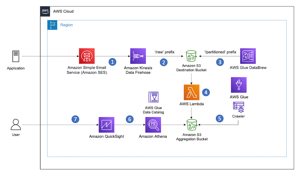
Track the usage of AWS Service Catalog products by analyzing the corresponding AWS CloudTrail logs. The latter can be forwarded to an Amazon EventBridge rule with a filter on the following events: CreateProduct, UpdateProduct, DeleteProduct, ProvisionProduct and TerminateProvisionedProduct.
The logs are generated no matter how you interact with the AWS Service Catalog API, such as through ServiceNow or TerraForm. Once in EventBridge, Amazon Kinesis Data Firehose delivers the events to Amazon Simple Storage Service (Amazon S3) from where QuickSight can access them. Figure 2 depicts the end-to-end flow.
Figure 2. Tracking adoption of AWS Service Catalog products with Amazon QuickSight
Depending on your AWS landing zone setup, CloudTrail logs from all relevant AWS accounts and regions need to be forwarded to a central S3 bucket in your shared services account or, otherwise, centralized logging account. Figure 3 provides an overview of this cross-account log aggregation.

Figure 3. Aggregating AWS Service Catalog product logs across AWS accounts
If your landing zone allows, consider giving permissions to EventBridge in all accounts to write to a central event bus in your shared services AWS account. This avoids having to set up Kinesis Data Firehose delivery streams in all participating AWS accounts and further simplifies the solution (Figure 4).

Figure 4. Aggregating AWS Service Catalog product logs across AWS accounts to a central event bus
If you are already using an organization trail, you can use Amazon Athena or AWS Lambda to discover the relevant logs in your QuickSight dashboard, without the need to integrate with EventBridge and Kinesis Data Firehose.
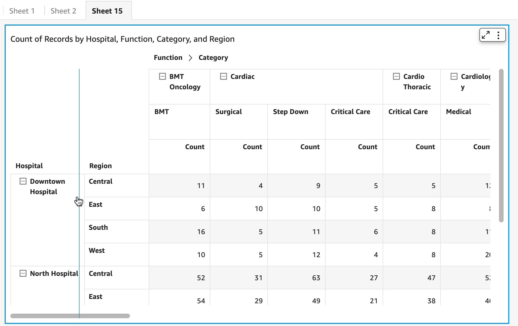
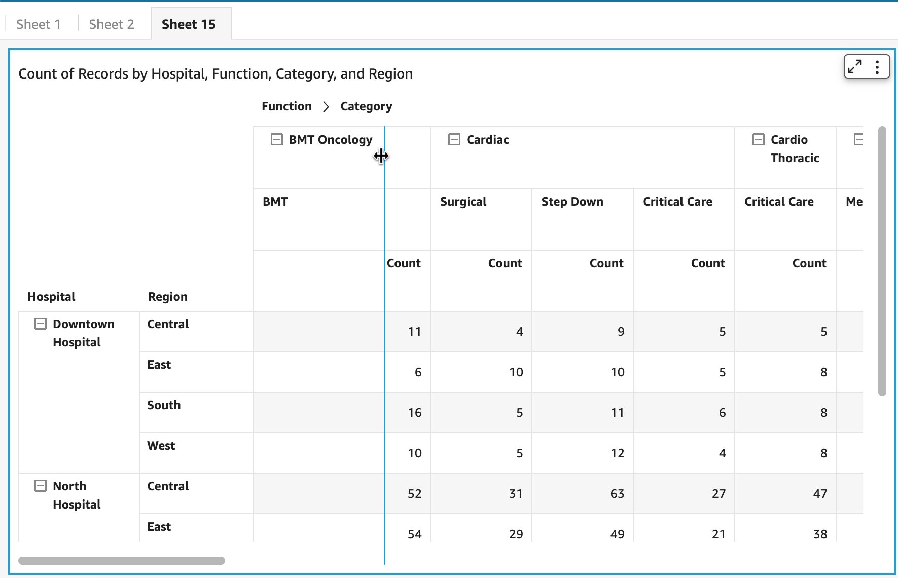
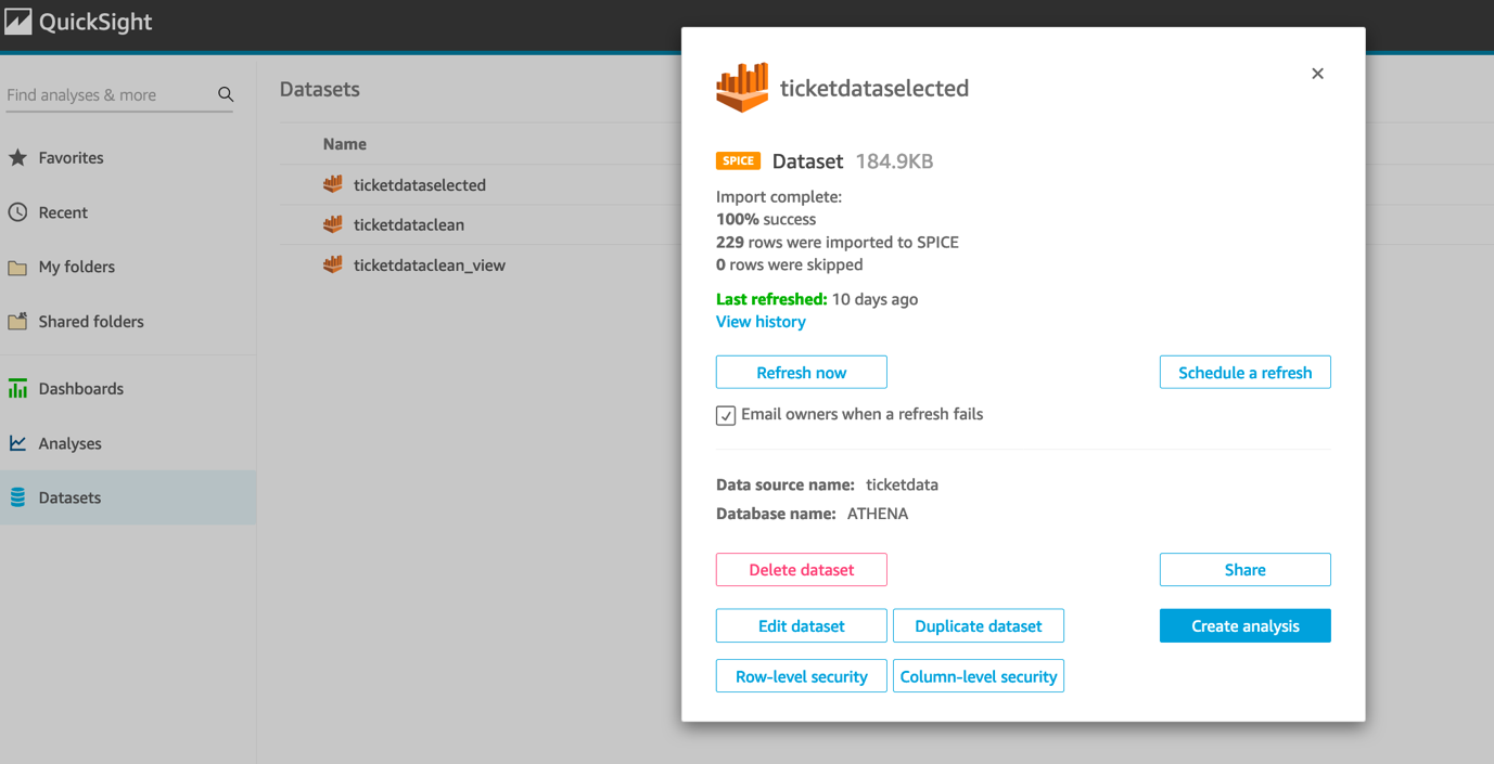
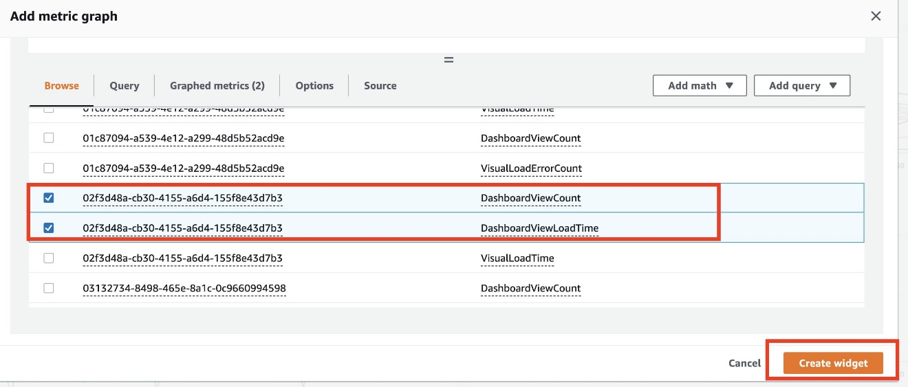
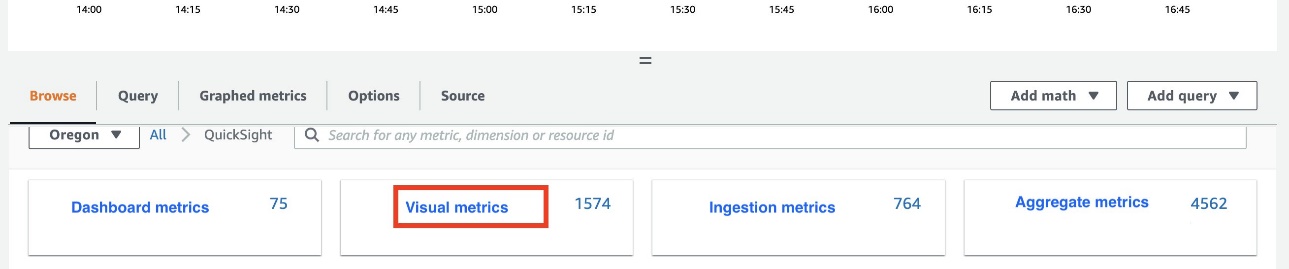
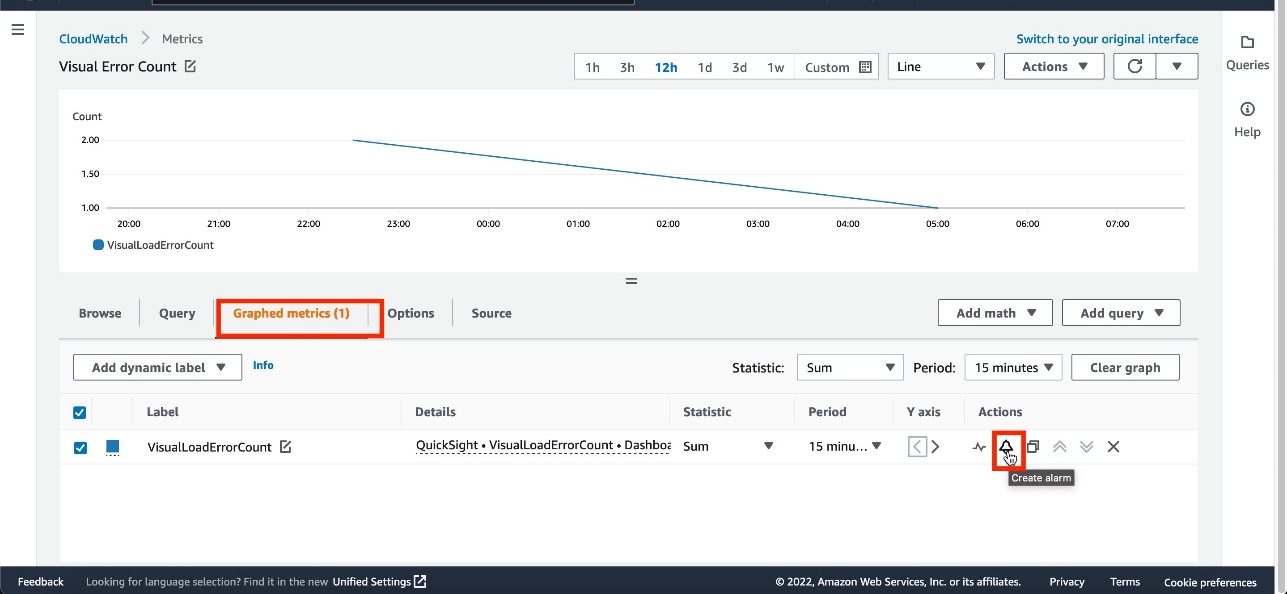
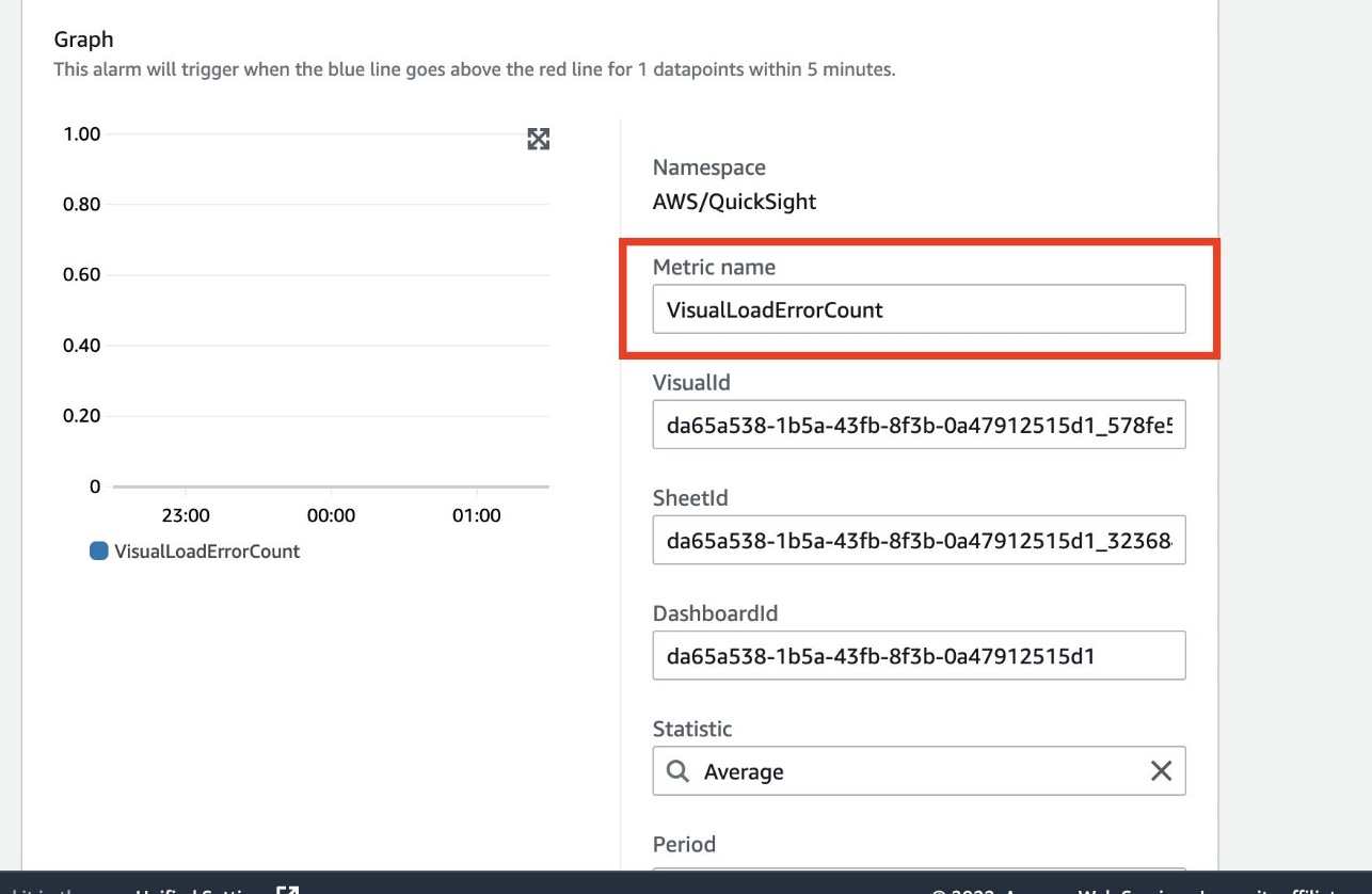
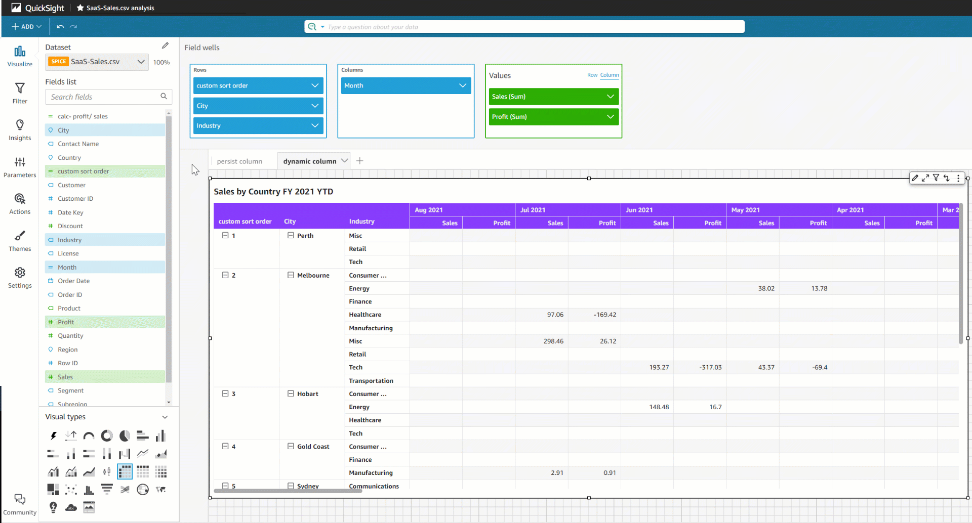
Reporting on product adoption can be customized in QuickSight. The S3 bucket storing AWS Service Catalog logs can be defined in QuickSight as datasets, for which you can create an analysis and publish as a dashboard.
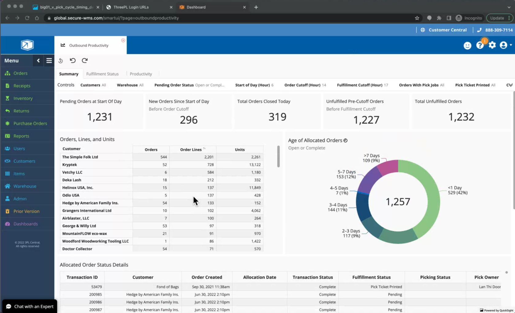
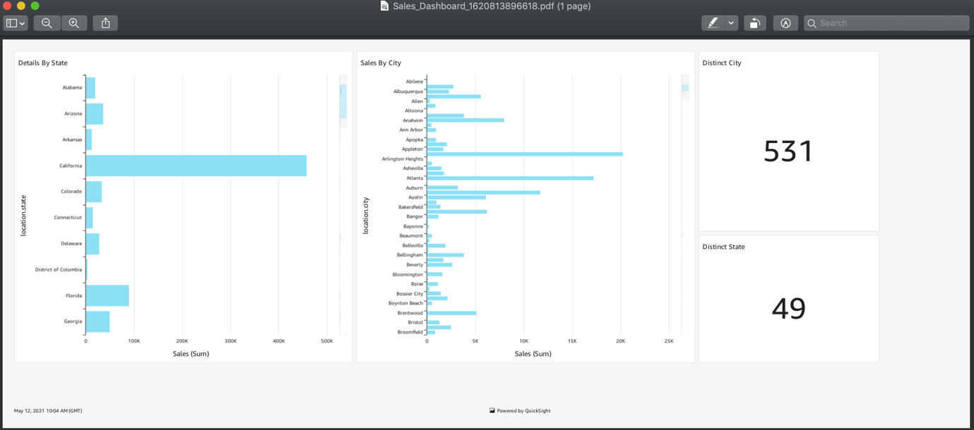
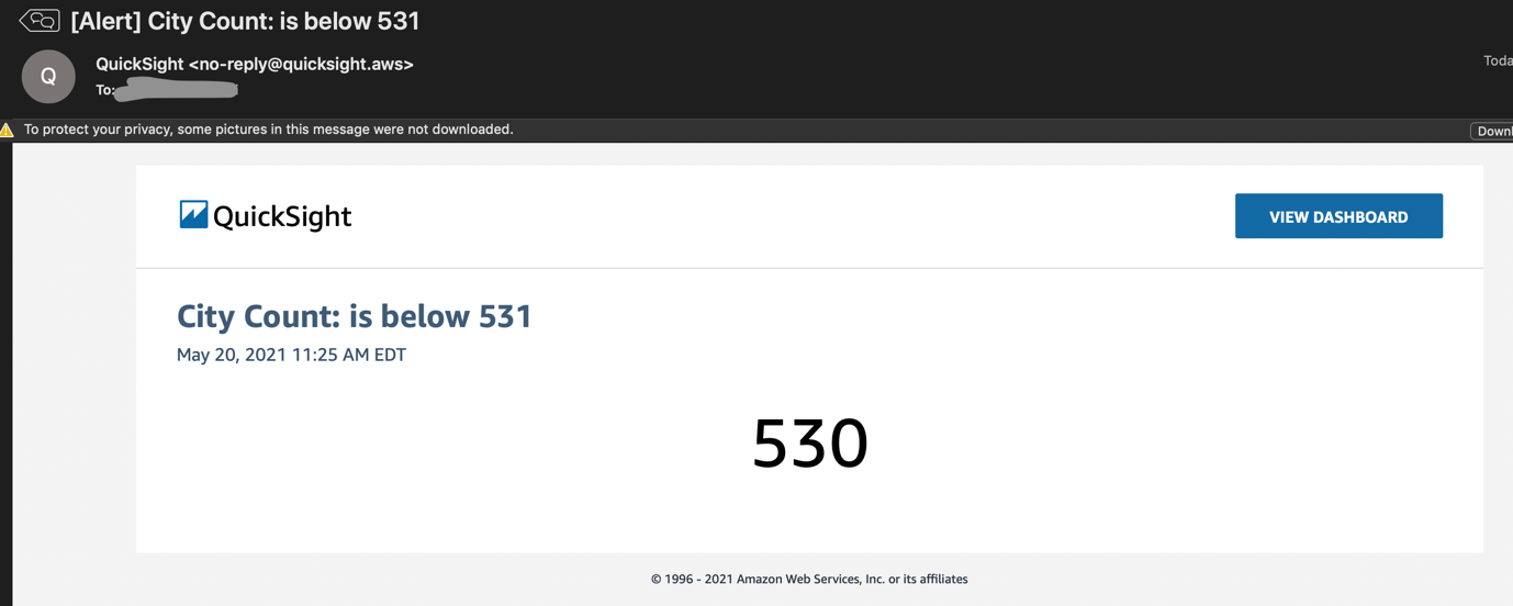
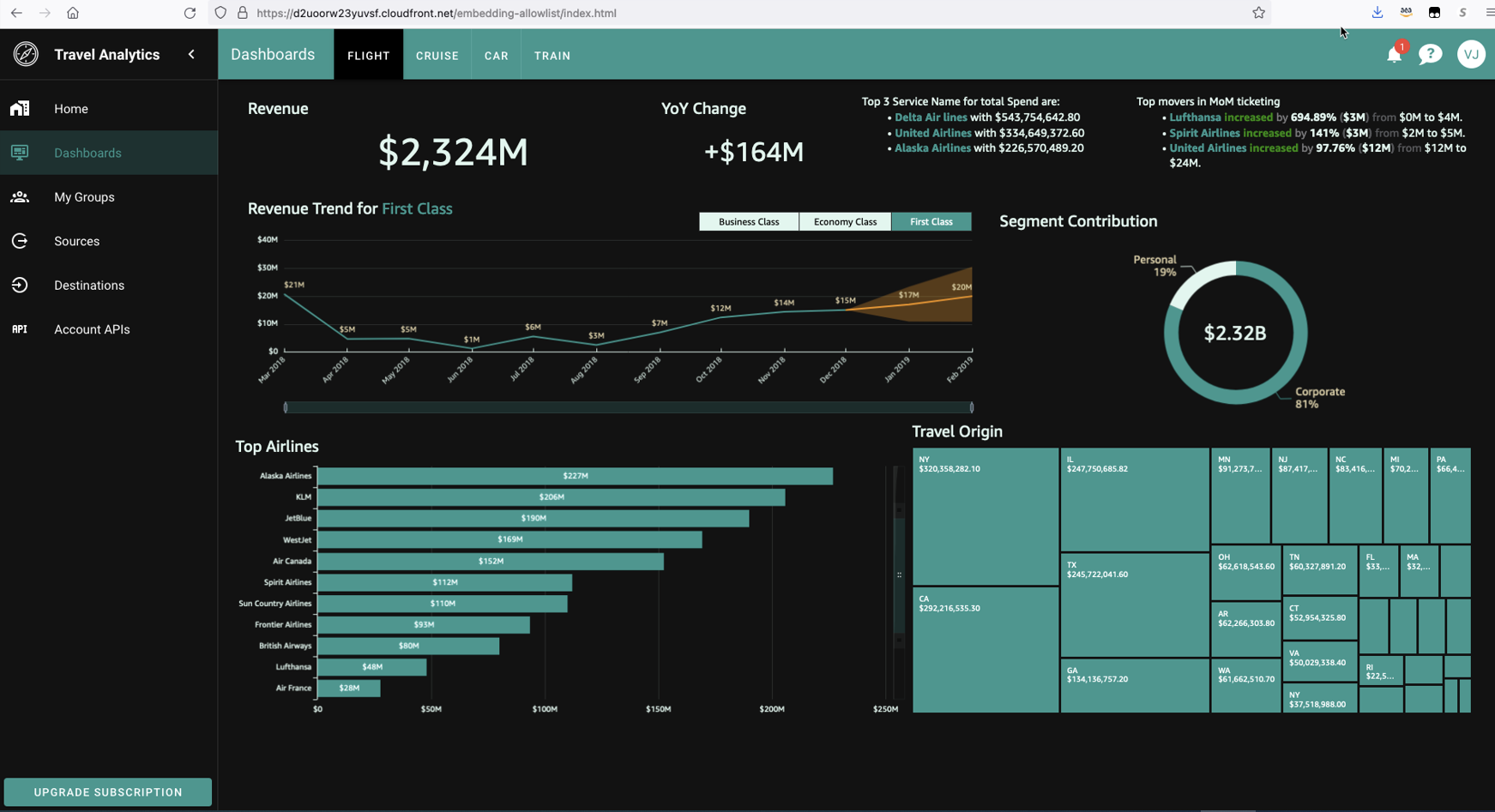
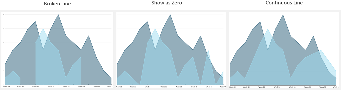
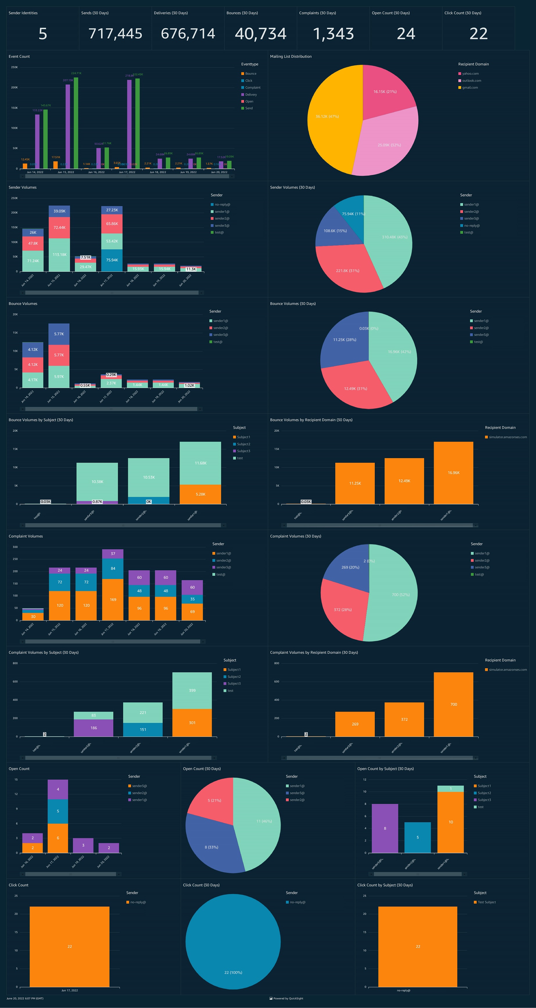
In the past, we have reported on the top ten products used in the organization (if relevant, also filtered by product version or time period) and the top accounts in terms of product usage. The following figure offers an example dashboard visualizing product usage by product type and number of times they were provisioned. Note: the counts of provisioned and terminated products differ slightly, as logging was activated after the first products were created and provisioned for demonstration purposes.
Figure 5. Example Amazon QuickSight dashboard tracking AWS Service Catalog product adoption
Conclusion
In this blog, we described an integrated approach to track adoption of cloud architecture patterns using AWS Service Catalog and QuickSight. The solution has a number of benefits, including:
- Building an IT service catalog based on pre-approved architectural patterns
- Maintaining visibility into the actual use of patterns, including which patterns and versions were deployed in the organizational units’ AWS accounts
- Compliance with organizational standards, as architectural patterns are codified in the catalog
In our experience, the model may compromise on agility if you enforce a high level of standardization and only allow the use of a few patterns. However, there is the potential for proliferation of products, with many templates differing slightly without a central governance over the catalog. Ideally, cloud platform engineers assume responsibility for the roadmap of service catalog products, with formal intake mechanisms and feedback loops to account for builders’ localization requests.


 Under Map Attributes, there should be four attributes.


 On the Attribute Mappings tab, you now add or update the attributes as in the following table.
 Srikanth Baheti is a Specialized World Wide Sr. Solution Architect for Amazon QuickSight. He started his career as a consultant and worked for multiple private and government organizations. Later he worked for PerkinElmer Health and Sciences & eResearch Technology Inc, where he was responsible for designing and developing high traffic web applications, highly scalable and maintainable data pipelines for reporting platforms using AWS services and Serverless computing.
 Raji Sivasubramaniam is a Sr. Solutions Architect at AWS, focusing on Analytics. Raji is specialized in architecting end-to-end Enterprise Data Management, Business Intelligence and Analytics solutions for Fortune 500 and Fortune 100 companies across the globe. She has in-depth experience in integrated healthcare data and analytics with wide variety of healthcare datasets including managed market, physician targeting and patient analytics.
 Raj Jayaraman is a Senior Specialist Solutions Architect for Amazon QuickSight. Raj focuses on helping customers develop sample dashboards, embed analytics and adopt BI design patterns and best practices.
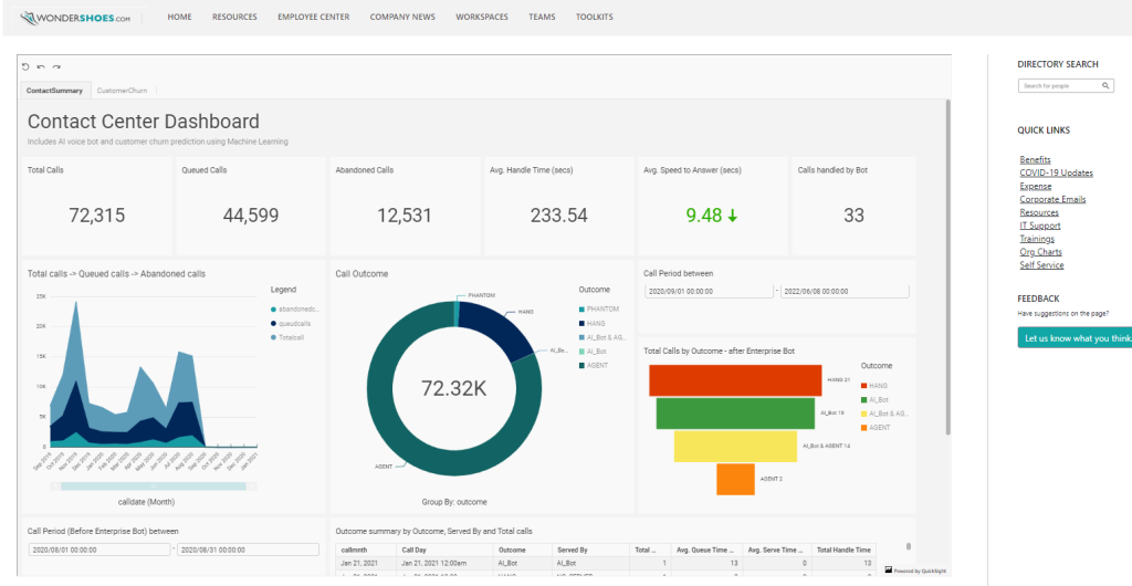
 Sindhu Chandra is a Senior Product Marketing Manager for Amazon QuickSight, AWS’ cloud-native, business intelligence (BI) service that delivers easy-to-understand insights to anyone, wherever they are.