Tag Archives: announcements

AWS DevOps Agent adds release management capabilities to assess code changes before production (preview)

Post Syndicated from Esra Kayabali original https://aws.amazon.com/blogs/aws/aws-devops-agent-adds-release-management-capabilities-to-assess-code-changes-before-production-preview/

Today, we’re announcing a new release management capability in AWS DevOps Agent that is now available in preview. AWS DevOps Agent is your always-available teammate that spans software changes and operations across AWS, multicloud, and on-premises environments. The practice of DevOps aims to make software change and operations smooth and increasingly autonomous, and AWS DevOps Agent delivers on both by leveraging its deep understanding of your environment, your services, their dependencies, and how they behave in production. Already generally available for post-deployment operations, it autonomously investigates incidents, provides root cause analysis and mitigation steps, and delivers targeted recommendations to prevent recurring issues. With today’s preview, AWS DevOps Agent adds release readiness review of code changes and autonomous release testing. These new features verify every change against the natural language standards you give to the DevOps Agent and run change-specific tests in production-like environments. AWS DevOps Agent now supports teams from code creation to production, helping reviewers and testers keep pace with the volume of AI-generated code.

As development teams adopt AI coding tools, the volume of pull requests moving through delivery pipelines has increased faster than review and testing processes can handle. When teams are under pressure to keep up, reviews are approved without thorough examination, and test environments drift from production. The value that coding agents generate sits waiting in review queues instead of reaching end users. At the same time, AI models are increasingly capable of catching functional and security issues that human reviewers might miss under time pressure, making speedy and safe delivery a requirement rather than a tradeoff.

The release readiness review feature evaluates every code change against production requirements, dependency safety, and the standards and best practices you provide to the DevOps Agent. The agent checks cross-repository dependency risks that could affect other services, access control changes against AWS Well-Architected Framework best practices, and compliance with any standards you have defined. When no standards are provided, the agent applies general best practices. As part of the review, the agent also runs your software in an AWS-managed isolated environment, executing lightweight user journey tests to verify the software builds, runs, and passes basic functional checks before the change enters the pipeline. Findings appear in the AWS DevOps Agent console and as comments on pull requests in GitHub or GitLab. You can also invoke reviews directly from your IDE through the Kiro power or Claude Code plugin, so developers can identify and fix dependency risks, standards violations, and access control issues before the change is committed to version control.

The autonomous release testing feature goes further, generating and running change-specific test plans for web and API-based applications in customer-provisioned, production-like environments before the change merges. Rather than running a static test suite, the agent reasons about what the change does and constructs tests tailored to it, covering functional correctness, behavioral regressions, and integration scenarios that a manually maintained test plan might not anticipate. Every test run produces structured artifacts including metrics, logs, traces, and an execution summary, giving reviewers a consistent record of what was tested and what the results were.

Getting started with AWS DevOps Agent release management
This walkthrough shows how to run an on-demand release readiness review using the AWS DevOps Agent web app. Before you begin, confirm that you have at least one GitHub or GitLab repository connected to your Agent Space. Once your repositories are connected, AWS DevOps Agent will index your code and build a knowledge graph of cross-repository and cloud dependencies.

To open the web app, navigate to the AWS DevOps Agent console, select your Agent Space, and choose the Web app tab. Choose Operator access to open the web app.

Without standards configured, the agent applies general best practices. To tailor reviews to your internal standards, navigate to Knowledge, then choose the Instructions tab. You will see a list of instruction sets, each scoped to a specific agent or task. Choose View next to Release readiness review to edit the instructions for production-readiness change review. Write your internal standards in plain English. For example, you can define infrastructure and data standards on encryption or network access rules, best practices that warn without blocking such as logging and observability requirements, and sensitive data classification best practices that identify applications or resources requiring higher security measures. To apply instructions across all agents in your space, choose View next to All agents.

You can trigger a release readiness review in two ways: by submitting a pull request to a connected repository, or by entering an on-demand query in the chat interface. To run an on-demand review from chat, choose New chat and enter a request such as:

Perform a production risk analysis on my repository branch

The agent will ask for the repository and branch you want to analyze. You can provide a branch name, a pull request number, or a commit SHA. Once you confirm your selection, the agent queues the review and analyzes the change for production risks, including infrastructure impacts, configuration changes, and potential issues.

After the review completes, you can ask follow-up questions directly in the chat to explore the findings in more detail. For example, you can ask which downstream consumers a change affects, and the agent will return a structured breakdown of in-repository and cross-repository consumers that will break, the specific files and line numbers affected, and the recommended steps to resolve the issue before deployment.

After submitting a review request, navigate to Changes in the left navigation pane. The Proposed changes table shows each review that has run, including the proposed change description, its source, category, status, and when it was created. You can filter by category or status to find specific reviews, or search by name using the search bar. Choose any entry to open the full execution detail.

The Timeline tab shows the agent’s step-by-step reasoning process, including the tools it called, the dependencies it consulted, and the observations it made at each step. Each entry is timestamped, giving you a complete record of how the agent built its understanding of the change and reached its conclusion.

Choose the Report tab to see the final recommendation. The report opens with a summary header showing the recommended action, the number of critical issues found, the commit revision, and the number of files changed. The recommended action is either BLOCK, Proceed with Caution, or Safe to Release.

Below the summary header, the Analysis section explains why the recommendation was made, citing specific risks and the evidence the agent found to support its conclusion. The Issues section lists each finding by severity, giving you a prioritized view of what needs to be addressed before the change can proceed. The Recommendations section provides specific, actionable steps the developer can take to resolve each issue. Finally, the Changes section lists each file that was modified, with the type of change, the category it falls under, and a description of what was changed, so reviewers have a complete picture of what the change does before it merges.

You can also invoke the autonomous release testing feature directly from the chat interface. To run an autonomous release test on a web or API-based application, choose New chat and enter a query such as:

Run a release test on my application deployed at [application URL]

The agent generates a change-specific test plan and executes it in your provisioned environment. Results appear in Changes, where you can review the execution steps and a structured summary of what was tested.

Get started today
The release readiness review and autonomous release testing features for AWS DevOps Agent are available in preview. These features are available at no additional cost during preview in the US East (N. Virginia) Region. For pricing information on other AWS DevOps Agent features, visit the AWS DevOps Agent pricing page.

For configuration details, visit the AWS DevOps Agent user guide.

— Esra

AI-assisted data development with Kiro and SageMaker Unified Studio

Post Syndicated from Zach Mitchell original https://aws.amazon.com/blogs/big-data/ai-assisted-data-development-with-kiro-and-sagemaker-unified-studio/

AI coding assistants are transforming software development, but data engineering presents unique challenges: governed data access, shared compute environments, and compliance controls that are designed to remain in place. How do you bring the power of agentic AI development into a governed data environment? With the AWS Toolkit for Visual Studio Code, you can connect Kiro, VS Code, or Cursor directly to Amazon SageMaker Unified Studio.

When you connect your editor to a SageMaker Unified Studio Space (a cloud-based compute environment inside your project), you get AI-assisted development with your preferred tools while your data governance, project permissions, and compute are managed by SageMaker Unified Studio. Additionally, SageMaker Unified Studio automatically generates steering files (like AGENTS.md) that provide your AI assistant with context about your project environment, so it understands your data and project configuration from the first prompt.

This post demonstrates the integration using Kiro. The same Remote Access connection works with VS Code and Cursor. The post starts by showing what you can do with this integration: using natural language to explore and analyze data in a governed environment. We then walk through the setup so you can try it yourself.

What’s new

With the AWS Toolkit, you can connect Kiro, VS Code, and Cursor to your SageMaker Space over a secure SSH tunnel. No additional extensions or SSH key management required. After the connection is established, your IDE has full access to your Space’s file system, compute, and data services.

Two capabilities make this especially powerful for data work:

  • Automatic AI steering – When connecting Kiro to SageMaker Unified Studio,  Kiro generates AGENTS.md and smus-context.md files that provide your AI assistant with context about your environment, including project configuration, environment details, and utilities for discovering your data catalog and project structure. Kiro detects these files automatically; other editors can use them as context for their own AI features.
  • MCP server support – have Kiro discover and configure itself for the Model Context Protocol servers on your remote SageMaker space ( like smus_local and aws-dataprocessing) to give your agent direct access to your AWS Glue Data Catalog, Amazon Athena queries, and SageMaker Unified Studio project metadata.

The following diagram shows how the components connect:

Architecture diagram: How the components connect

See it in action: AI-assisted development with governed data

Before walking through the setup, we explain what you can do with this integration. This walkthrough uses Kiro as the editor. With Kiro connected to a SageMaker Unified Studio Space, MCP servers configured, and steering documents in place, we can use natural language to explore data and build analytics. The AI assistant has all the context it needs to do this well.

Note: Agentic AI output is nondeterministic. The exact code, tool choices, and responses Kiro produces will vary between sessions, even with the same prompt. The following walkthrough shows one representative session. Your experience will differ in the specifics, but the patterns and capabilities demonstrated here are consistent.

Step 1: Explore the data

Start with a simple prompt:

show my databases and the tables I have access to

Even with native MCP tools available, Kiro often prefers the AWS Command Line Interface (AWS CLI) and bash to retrieve information. This is expected and typically does not affect the outcome. If you prefer MCP tools for every operation, you can add that preference to a steering document.

Kiro used the sagemaker_studio SDK to discover the catalog:

python3 -c "
from sagemaker_studio import Project
project = Project()
conn = project.connection()
catalog = conn.catalog()
print('Databases:')
for db in catalog.databases:
    print(f'  - {db.name}')
"
Databases:
  - default
  - sagemaker_sample_db

Then it drilled into the table schema:

python3 -c "
from sagemaker_studio import Project
project = Project()
conn = project.connection()
catalog = conn.catalog()
db = catalog.database('sagemaker_sample_db')
print('Tables in sagemaker_sample_db:')
for t in db.tables:
    print(f'  - {t.name}')
    print(f'    Columns: {[(c.name, c.type) for c in t.columns]}')
"
Tables in sagemaker_sample_db:
  - churn
    Columns: [('state', 'string'), ('account_length', 'int'),
              ('area_code', 'string'), ('phone', 'string'),
              ('intl_plan', 'string'), ('vmail_plan', 'string'),
              ('vmail_message', 'int'), ('day_mins', 'double'),
              ('day_calls', 'int'), ('day_charge', 'double'),
              ('eve_mins', 'double'), ('eve_calls', 'int'),
              ('eve_charge', 'double'), ('night_mins', 'double'),
              ('night_calls', 'int'), ('night_charge', 'double'),
              ('intl_mins', 'double'), ('intl_calls', 'int'),
              ('intl_charge', 'double'), ('custserv_calls', 'int'),
              ('churn', 'boolean')]

Kiro discovered the sagemaker_sample_db.churn dataset, a sample dataset that ships with SageMaker Unified Studio containing 10,000 rows and 21 columns of customer churn data (state, account length, call minutes, service calls, churn flag, and more). Notice that we did not write any of this code. We asked a question in natural language, and Kiro chose the right SDK calls, explored the catalog, and surfaced the results.

Another, more natural way to get the same answer is to ask directly. Prompting “Let us sample the churn table.” yields the same catalog paths and schema output, along with additional metrics like row count and a data sample, all from a single conversational prompt:

SageMaker Unified Studio console showing the sagemaker_sample_db.churn dataset listed in the catalog

Figure 1 — The sagemaker_sample_db.churn dataset in the catalog

Schema view showing the 21 columns of the churn table including state, account_length, call minutes, and the churn boolean

Figure 2 — Churn dataset schema with 21 columns

from sagemaker_studio import sqlutils
result = sqlutils.sql(
    'SELECT COUNT(*) AS total_rows FROM sagemaker_sample_db.churn',
    connection_name='default.sql'
)
print('=== Total Row Count ===')
print(result)
=== Total Row Count ===
   total_rows
0       10000

With the schema and row count in hand, Kiro sampled the data to round out its understanding of the dataset:

Comprehensive data sample showing 10 rows from the churn table with all 21 columns populated

Figure 3 — Comprehensive data sample after Kiro catalog exploration

Step 2: Run analytics with full context

With the data explored, ask Kiro to run a data quality evaluation:

Can we run basic statistical evaluations for data quality?

Because Kiro had already explored the catalog and sampled the data, it made smart choices about how to run the analysis. Instead of using PySpark for this 10,000-row table, Kiro used Athena using sqlutils to run the evaluation directly. It produced a thorough data quality report:

  • 10,000 rows, 21 columns, zero nulls across all columns. Clean on that front.
  • 5,000 duplicate rows (50 percent). Significant, worth investigating before modeling.
  • Outliers minimal. Most columns have less than 1 percent outlier rate by IQR.
  • Churn is nearly 50/50 split (50.04 percent False, 49.96 percent True). Unusually balanced, indicating synthetic data.
  • Clear signal in key features. Churners and non-churners show differences in day_mins (7.52 vs. 3.52), eve_mins (5.95 vs. 4.11), and vmail_message (175 vs. 278).
  • State distribution roughly uniform (~2% each), intl_plan and vmail_plan near 50/50.

The key insight here is what Kiro did not do. It did not default to PySpark because the environment supports Spark. Having explored the data first, understanding the table size, column types, and that churn is a proper Boolean (not a string), Kiro independently chose the right engine for the workload and produced correct analytics on the first pass.

Best practice: Explore first, code second

Start every AI-assisted development session with data exploration. Ask your AI assistant to discover your catalog, sample your tables, and understand the schema before asking it to build anything. This single step helps reduce a common source of errors in AI-assisted data work: the LLM making assumptions about data it has not seen.

Exploring your data gives the large language model (LLM) the context it needs to properly help with your project. It saves hallucinations and rework, results in faster development time, and reduces token costs.

Ready to try it yourself? The following sections walk through the full setup: prerequisites, connecting your editor to your SageMaker Space, configuring MCP servers, and working with notebooks.

Prerequisites

Before you begin, make sure you have the following:

  • A SageMaker Unified Studio domain and project with at least one project that has a compute environment provisioned (Tooling or ToolingLight). These should come standard with every SageMaker project except those provisioned with the SQL & Gen AI blueprints. If you need to set up SageMaker Unified Studio, see Getting started with Amazon SageMaker Unified Studio.
  • A Space with Remote Access enabled. Either a JupyterLab or Code Editor Space works. The instance must have at least 8 GiB of memory (for example, ml.t3.large or larger). The default ml.t3.medium (4 GiB) can’t enable Remote Access. You must upgrade the instance type first, then toggle Remote Access to Enabled in the Configure Space dialog.
  • A VS Code-compatible editor. Kiro, VS Code, Cursor, or another VS Code-based IDE installed on your local machine. This walkthrough uses Kiro, but the Remote Access connection has been tested with VS Code and Cursor as well.
  • AWS Toolkit v4.1.0 or later. Kiro ships with the AWS Toolkit pre-installed. For VS Code and Cursor, install the AWS Toolkit extension and verify your version is 4.1.0 or later (Cmd+Shift+X and search for “AWS Toolkit”).
  • AWS credentials. You must be authenticated in the SageMaker Unified Studio panel of the AWS Toolkit with the same identity (AWS IAM Identity Center or AWS Identity and Access Management (IAM)) that you use to access SageMaker Unified Studio in the browser.
  • Network connectivity. Your Space must have internet access (PublicInternetOnly mode, or virtual private cloud (VPC) with a NAT gateway or HTTP proxy that allows VS Code and Open VSX endpoints).

The following screenshots show the SageMaker Unified Studio portal and the Configure Space dialog. Navigate to your project, select your Space, and verify the configuration. Remote Access is disabled when the instance has less than 8 GiB of memory. Select an instance with at least 8 GiB, such as ml.t3.large, then enable Remote Access. This is a one-time configuration per Space.

SageMaker Unified Studio portal showing the Spaces list for a project

Figure 4 — SMUS project Spaces overview in the portal

Configure Space dialog with the instance type selector open and ml.t3.large highlighted

Figure 5 — Configure Space dialog showing instance type selection

Configure Space dialog with the Remote Access toggle set to Enabled on an 8 GiB instance

Figure 6 — Enabling Remote Access on a Space with 8 GiB or more

Connecting your editor to your SageMaker Space

There are two ways to connect: directly from the SageMaker Unified Studio portal, or from your local IDE using the AWS Toolkit.

Method 1: Connect from the SageMaker Unified Studio portal

To launch your IDE directly from the portal, navigate to your project’s Code Spaces page, find your Space, and choose Open in to select your editor (Kiro, VS Code, or Cursor):

Code Spaces list with the Open in menu showing options for Kiro, VS Code, and Cursor

Figure 7 — Open in Local IDE from the Code Spaces list

You can also launch from within a Space’s details page:

Space details page with the Open in menu expanded

Figure 8 — Open in Local IDE from the Space details page

Or from within the JupyterLab or Code Editor browser environment:

JupyterLab toolbar with the Open in Local IDE option visible

Figure 9 — Open in Local IDE from JupyterLab

Your browser will prompt you to allow opening the IDE. Confirm, and the editor launches with an SSH connection to your Space already established via the AWS Toolkit. No additional configuration is typically required.

Method 2: Connect from your IDE via the AWS Toolkit

  1. Open your editor on your local machine. Then, in the AWS Toolkit panel, choose Sign in. Authenticate with your IAM Identity Center or IAM credentials, the same identity you use to access SageMaker Unified Studio in the browser. The following screenshots show Kiro, but the steps are the same in VS Code and Cursor.Figure 10 — AWS Toolkit button in Kiro
    Figure 10 — AWS Toolkit button in KiroAWS Toolkit panel expanded in Kiro showing the Sign in option

    Figure 11 — AWS Toolkit panel expanded

    AWS Toolkit Sign in dialog with profile selection

    Figure 12 — AWS Toolkit Sign in dialog

  2. Choose your AWS profile. You must have a profile configured in the AWS CLI with the correct account and AWS Region set.
  3. In the Toolkit panel, browse your SageMaker Unified Studio domains and projects. Select the project that you want to work in.

Kiro AWS Toolkit panel showing SageMaker Unified Studio domains and projects in a tree view

Figure 13 — Browsing SMUS domains and projects in Kiro

Important: The credentials that you use in the AWS Toolkit must match the identity that you use in the SageMaker Unified Studio portal. The Toolkit validates that your identity has access to the Space.

AI steering: How SageMaker Unified Studio pre-seeds AI context

The real value of the feature comes from what you don’t need to do. When connected to Kiro SageMaker Unified Studio automatically generates steering files that guide your AI assistant with project context, so you can focus on building analytics rather than configuring connections. When you open a SageMaker Unified Studio project, SageMaker Unified Studio presents a prompt to create steering files: an AGENTS.md file that references a newly created smus-context.md. These files provide context about your project environment, such as project configuration, environment details, and utilities for discovering your data catalog and project structure. Kiro detects and applies these files automatically; in other editors, you can reference them as context for your AI features.

SageMaker Unified Studio popup offering to create AGENTS.md and smus-context.md steering files

Figure 14 — SMUS popup offering to create steering files

Kiro file explorer showing the generated AGENTS.md and smus-context.md files at the project root

Figure 15 — Generated AGENTS.md and smus-context.md steering files

Without these steering files, your AI assistant would need several back-and-forth prompts to discover what data you have and how to access it. With them, the assistant understands your project from the first prompt: how to discover your databases, how your environment is configured, and what tools are available. The steering files also help properly configure MCP servers, which you set up in the next section.

Exploring your project

After you’re connected, the project structure expands into Data and Compute sections in the sidebar, as it would in the SageMaker Unified Studio portal.

Kiro sidebar showing the Data and Compute sections expanded under a SageMaker Unified Studio project

Figure 16 — Project Data and Compute sections in the Kiro sidebar

You can explore your data catalog and S3 buckets directly from the sidebar:

Kiro sidebar with the data catalog tree and S3 buckets expanded under the project

Figure 17 — Exploring the data catalog and S3 buckets from the sidebar

You can also remote into a compatible Space for direct development. Hover over a Space and select the remote icon on the right:

Kiro sidebar showing the remote connection icon next to a compatible Space

Figure 18 — Remote connection icon on a compatible Space

After a moment, the Space opens in a new Kiro window:

New Kiro window opened with a remote connection to the SageMaker Unified Studio Space

Figure 19 — Space opened in a new Kiro window

You must sign in again, and then trust the authors of the files in the Space:

Trust authors dialog asking to confirm trust for files in the remote Space

Figure 20 — Trust authors dialog for the Space files

You’re now connected to your Space. The Toolkit works on the Space the way it does locally, except the resources are scoped to the project’s permissions.

Kiro window connected to a SageMaker Unified Studio Space with the AWS Toolkit panel active

Figure 21 — Connected to the SMUS Space with the Toolkit active

Setting up MCP servers

Before you can use AI-assisted development effectively, you must give Kiro access to your data services through Model Context Protocol (MCP) servers. MCP servers extend the Kiro agent with tools: the ability to query catalogs, run SQL, manage credentials, and more.

Out of the box, Kiro has no MCP servers configured:

Kiro MCP servers panel with no servers configured

Figure 22 — Kiro MCP servers panel with no servers configured

Prompt Kiro to find and configure the MCP servers that ship pre-installed on your SageMaker Space. Using the steering file context, Kiro located the servers and generated the configuration. If a server fails to connect, select the failed entry and Kiro will suggest fixes. You might need additional prompts to get the smus_spark_upgrade server (a pre-installed MCP server for managing Spark session upgrades) working correctly.

Kiro chat panel showing the agent discovering and configuring SageMaker Unified Studio MCP servers

Figure 23 — Kiro discovering and configuring SMUS MCP servers

MCP servers panel after iterating on configuration fixes, showing servers connected

Figure 24 — MCP servers after iterating on configuration fixes

For more deterministic results, you can also configure the MCP servers manually. Here is a sample configuration:

{
    "mcpServers": {
        "smus_local": {
            "command": "python3",
            "args": ["-m", "sagemaker_studio.mcp_server"],
            "env": {}
        },
        "aws-dataprocessing": {
            "command": "uvx",
            "args": ["awslabs.aws-dataprocessing-mcp-server@latest"],
            "env": {
                "AWS_REGION": "us-east-1",
                "FASTMCP_LOG_LEVEL": "ERROR"
            },
            "disabled": ["emr_*"]
        }
    }
}

Note: Your MCP configuration might vary depending on your SageMaker Unified Studio environment. Use the preceding configuration as a starting point and let your editor adjust if a server fails to connect.

Next, add the AWS Data Processing MCP server to get catalog information and Athena query capabilities. This isn’t strictly required (Kiro can use Python or AWS CLI for the same tasks), but it gives the agent native tools for catalog and query operations.

AWS Data Processing MCP server tools listed in Kiro with the Amazon EMR tool group disabled

Figure 25 — AWS Data Processing MCP server tools with Amazon EMR tools disabled

You can list the tools that each MCP server provides. Because the AWS Data Processing MCP server includes tools for many services, we recommend disabling tools that you don’t need for a given project to save model context. For this walkthrough, disable the Amazon EMR tools to focus on AWS Glue and Amazon Athena.

Exploring data with notebooks

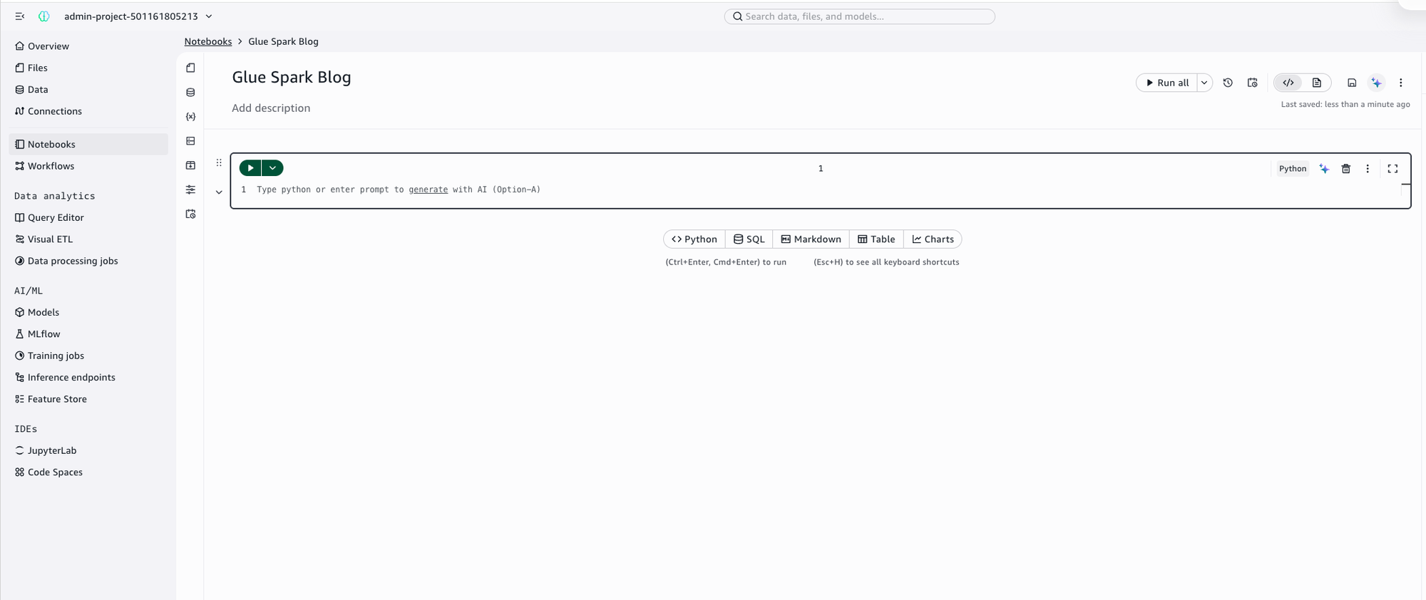
Kiro supports Jupyter notebooks in your SageMaker Space with the same language and connection selectors that you would find in SageMaker JupyterLab or Code Editor. Open the command palette (Cmd+Shift+P) and create a new Jupyter notebook:

Kiro command palette filtered to the Create New Jupyter Notebook command

Figure 26 — Command palette to create a new Jupyter notebook

New Jupyter notebook open in Kiro showing language and connection selectors at the bottom-right of a cell

Figure 27 — New Jupyter notebook opened in Kiro with language and connection selectors in a notebook cell

As in SageMaker JupyterLab, you get language and connection selectors in the bottom right of each cell. Choose the connection selector to see your available connections:

SageMaker connection selector dropdown showing the available connections for the project

Figure 28 — SageMaker connection selector

Select PySpark to fill in the magic commands for your cell. Write your code (in this case, enter spark and press Shift+Enter) to verify the session starts:

Notebook cell prefilled with the PySpark magic command and a spark verification statement

Figure 29 — PySpark magic command and spark verification code

PySpark cell running in the Kiro notebook

Figure 30 — Running the PySpark cell

If this is your first time using Jupyter with Kiro, you’re prompted to install the Jupyter extension. After it’s installed, select the kernel from Python Environments → Base:

Jupyter kernel selection prompt in Kiro after installing the Jupyter extension

Figure 31 — Jupyter kernel selection prompt

Kernel picker showing the Python kernel selected from the Base environment

Figure 32 — Selecting the Python kernel from the Base environment

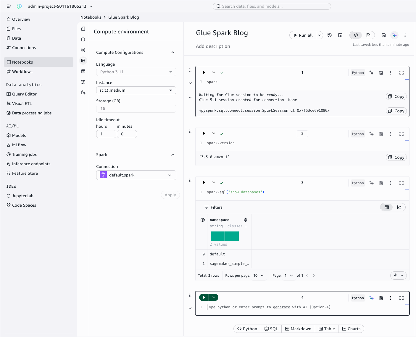
Re-run your cell. After a few moments, AWS Glue provisions a PySpark session:

AWS Glue provisioning a PySpark session in a Jupyter notebook in Kiro

Figure 33 — AWS Glue provisioning a PySpark session in a Jupyter notebook in Kiro

You see results the way you would in JupyterLab in the SageMaker Unified Studio portal:

PySpark code running in a Jupyter notebook in Kiro with output cells populated

Figure 34 — PySpark code running in a Jupyter notebook in Kiro

The notebook generate button

You will notice a Generate button underneath notebook cells. Let’s test it with a simple prompt:

looking at the above cell for reference, show me the accounts where state = california
using pyspark prefixing the cell with `%%pyspark default.spark` and sorting by
account_length

Notebook cell showing the Generate button populated with a natural language prompt

Figure 35 — Using the Generate button with a natural language prompt

Generated PySpark code populating a notebook cell after using the Generate button

Figure 36 — Generated PySpark code from the prompt

This prompt builder, like other notebook generation features, doesn’t have good context on the surrounding cells. You must be explicit about what you want because it won’t read other code or cells as input.

While the Kiro notebook generate button works for straightforward edits, for serious code generation, we recommend that you use Kiro agent mode. This mode has full project and SageMaker context, as demonstrated in the “See it in action” walkthrough earlier in this post.

What’s happening under the hood

When you connect your editor to a SageMaker Unified Studio Space, the AWS Toolkit extension establishes a secure SSH tunnel between your local IDE and your cloud-based Space.

Key details:

  • SSH tunnel. The connection is managed entirely by the AWS Toolkit (v4.1.0+) or VS Code’s built-in SSH extension. No separate Remote SSH extension is needed; the capability is built in.
  • File system access. Your editor sees the Space’s persistent storage at /home/sagemaker-user/, including shared project files and notebooks or scripts you create.
  • SageMaker Unified Studio steering context. The integration generates AGENTS.md and smus-context.md files that provide your AI assistant with context about your project environment and utilities for understanding your data. This is what makes the assistant effective from the first prompt.
  • MCP server integration. MCP servers like smus_local (for project metadata and environment utilities) and aws-dataprocessing (for AWS Glue Data Catalog and Amazon Athena) extend your editor’s AI with direct access to your data services. Your own MCP servers will be equally valuable here.
  • Credential flow. The Toolkit uses your existing AWS identity (IAM Identity Center or IAM) to authenticate to the Space. No separate SSH keys to manage. The aws_context_provider tool from the smus_local MCP server handles credential discovery for agent operations.

Best practices

To work effectively with your IDE and SageMaker Unified Studio:

  • Explore your data before building. Start every session by asking your AI assistant to discover your catalog, sample your data, and understand the schema. This single step helps reduce the most common source of errors in AI-assisted data work: the LLM making assumptions about data it has not seen. See the “See it in action” walkthrough earlier in this post for a concrete example of the difference this makes.
  • Use the SageMaker Unified Studio steering files. When prompted to create AGENTS.md and smus-context.md, accept. These files are the foundation that makes everything else work: environment context, MCP server configuration, and project understanding. Without them, your AI assistant starts from zero on every prompt. Kiro detects these automatically; in other editors, add them as context.
  • Disable unused MCP tools. The AWS Data Processing MCP server includes tools for AWS Glue, Amazon EMR, Amazon Athena, and more. Disable the services that you’re not using for a given project to save model context and reduce noise.
  • Be specific in your prompts. The more detail you give your AI (column names, query patterns you prefer, output formats), the closer the first pass will be. “Run data quality evaluation using Athena SQL” gets you better code than “check my data.”
  • Always test interactively first. Whether in notebooks or the terminal, validate code before deploying it. AI agents can iterate quickly, but catching issues in an interactive session is faster than debugging a failed AWS Glue job. Athena PySpark and the SageMaker sqlutils and sparkutils packages are great for this.
  • Stop your Space when idle. Your Space runs on compute (the same instance types as Code Editor and JupyterLab). If idle, the Space will terminate after 60 minutes and close your remote connection. Close the remote window and reconnect to continue.

Things to know

  • Notebook agent mode. For notebook-heavy analytics workflows where you want agentic AI to generate and run cells directly, SageMaker Notebooks with Data Agent in SageMaker Unified Studio is the recommended option today. Current notebook support in local editors covers editing, running, and generating code in individual cells.
  • MCP setup takes iteration. Configuring MCP servers may require iteration, especially for servers with complex authentication. Many AI-enabled editors can self-correct when a server fails. For more deterministic results, use the preceding MCP configuration JSON as a starting point rather than relying solely on auto-discovery.
  • CLI preference. AI agents often prefer the AWS CLI and bash even when MCP tools are available. This doesn’t affect outcomes, but you can steer your assistant toward MCP tools using a steering document if you prefer consistency.

Security and governance boundaries

A core benefit of this integration is that your existing security and governance controls remain enforced. Your editor connects to your SageMaker Space through a secure SSH tunnel managed by the AWS Toolkit. It does not bypass your organization’s access controls. Data access is governed by the same AWS Lake Formation permissions and IAM Identity Center authentication that apply when you work in the SageMaker Unified Studio portal directly. Your project-level permissions, database grants, and column-level security policies apply consistently whether a query originates from an AI agent, a notebook cell, or the SageMaker console. Data access is governed by the boundaries you define in your SageMaker Unified Studio domain and project configuration.

Clean up

To avoid ongoing charges from billable resources (SageMaker Space compute charges per hour, AWS Glue sessions charge per DPU-hour, Amazon Athena queries charge per TB scanned):

  1. Stop your Space – In the SageMaker Unified Studio portal, navigate to your project’s Spaces and stop the Space you used for this walkthrough.
  2. Disconnect: Close the remote connection in your editor (File → Close Remote Connection).
  3. Verify AWS Glue sessions are terminated – If you ran PySpark queries during this walkthrough, verify that the sessions are stopped. In the SageMaker Unified Studio portal, navigate to Data processing and confirm no active AWS Glue sessions remain. Sessions auto-terminate when the Space stops, but verify to avoid unexpected charges.
  4. Delete demo resources (optional) – File deletion is permanent and cannot be undone. Back up any work that you want to retain before proceeding. If you created scripts or files during this walkthrough that you no longer need, delete them from /home/sagemaker-user/. For example, delete any test notebooks, Python scripts, or generated data files. The sample sagemaker_sample_db.churn dataset is read-only and doesn’t need cleanup.

Conclusion

This post showed what happens when agentic AI meets governed data, and walked through how to set it up yourself.

Three key insights emerged from this hands-on experience:

  1. SageMaker Unified Studio steering files transform the developer experience. Your AI assistant is project-aware from the first prompt, understanding your environment and available data without manual setup.
  2. MCP servers bridge “AI that writes code” with “AI that queries your data”. The smus_local and aws-dataprocessing servers are essential for effective agentic data work.
  3. The “explore first” pattern pays immediate dividends. When your AI assistant understands your data before writing code, it makes smarter engine choices and produces correct analytics on the first pass.

This integration brings together two capabilities that are stronger together: your IDE handles the AI-assisted coding and iteration, while SageMaker Unified Studio handles data governance, access control, and compute management. You get the productivity of an agentic AI coding assistant without compromising on the controls your organization requires.

To get started, download Kiro, install VS Code or Cursor, and add the AWS Toolkit for Visual Studio Code (v4.1.0 or later). Then visit the Amazon SageMaker Unified Studio documentation and the AWS Data Processing MCP Server to set up your first Space. For related reading, see Speed up delivery of ML workloads using Code Editor in Amazon SageMaker Unified Studio.


About the authors

Zach Mitchell

Zach Mitchell

Zach is a Senior Big Data Architect in AWS Worldwide Specialist Organization for Analytics. He works with customers to design and build data applications on AWS, with a focus on SageMaker Unified Studio, AWS Glue, and AWS Lake Formation. Outside of work, he enjoys building things with code and occasionally writing about it.

Anchit Gupta

Anchit Gupta

Anchit is a Senior Product Manager on the Amazon SageMaker Unified Studio team at AWS.

Leah Wagner

Leah Wagner

Leah is a Senior Solutions Architect in AWS Worldwide Specialist Organization for Analytics.

Bhargava Varadharajan

Bhargava Varadharajan

Bhargava is a Senior Software Engineer on the Amazon SageMaker Unified Studio team at AWS.

Majisha Namath Parambath

Majisha Namath Parambath

Majisha is a Software Development Engineer on the Amazon SageMaker Unified Studio team at AWS.

Modernize Amazon Redshift: RA3 to RG Migration best practices

Post Syndicated from Nita Shah original https://aws.amazon.com/blogs/big-data/modernize-amazon-redshift-ra3-to-rg-migration-best-practices/

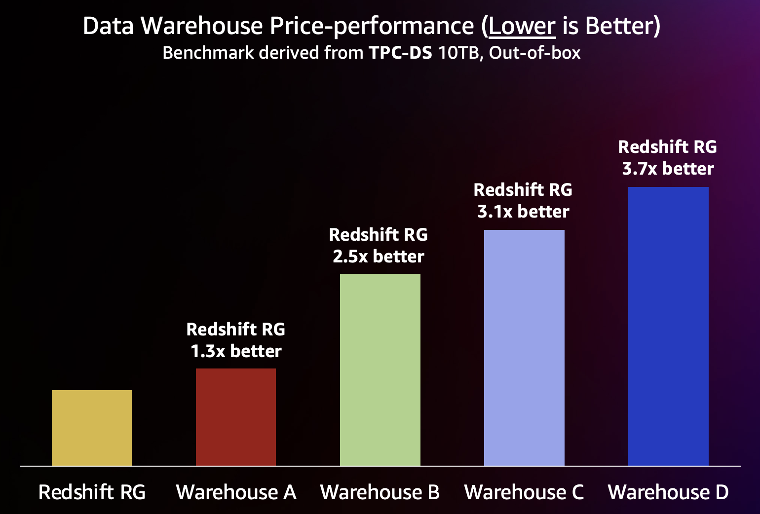
Amazon Redshift is a fully managed, AI-powered cloud data warehouse used by tens of thousands of customers to analyze exabytes of data with industry-leading price-performance. Amazon Redshift delivers SQL analytics across your entire lakehouse in Amazon SageMaker Unified Studio, unifying data from multiple sources. Zero-ETL integrations remove complex pipelines by connecting streaming, databases, and enterprise applications for near real-time insights.

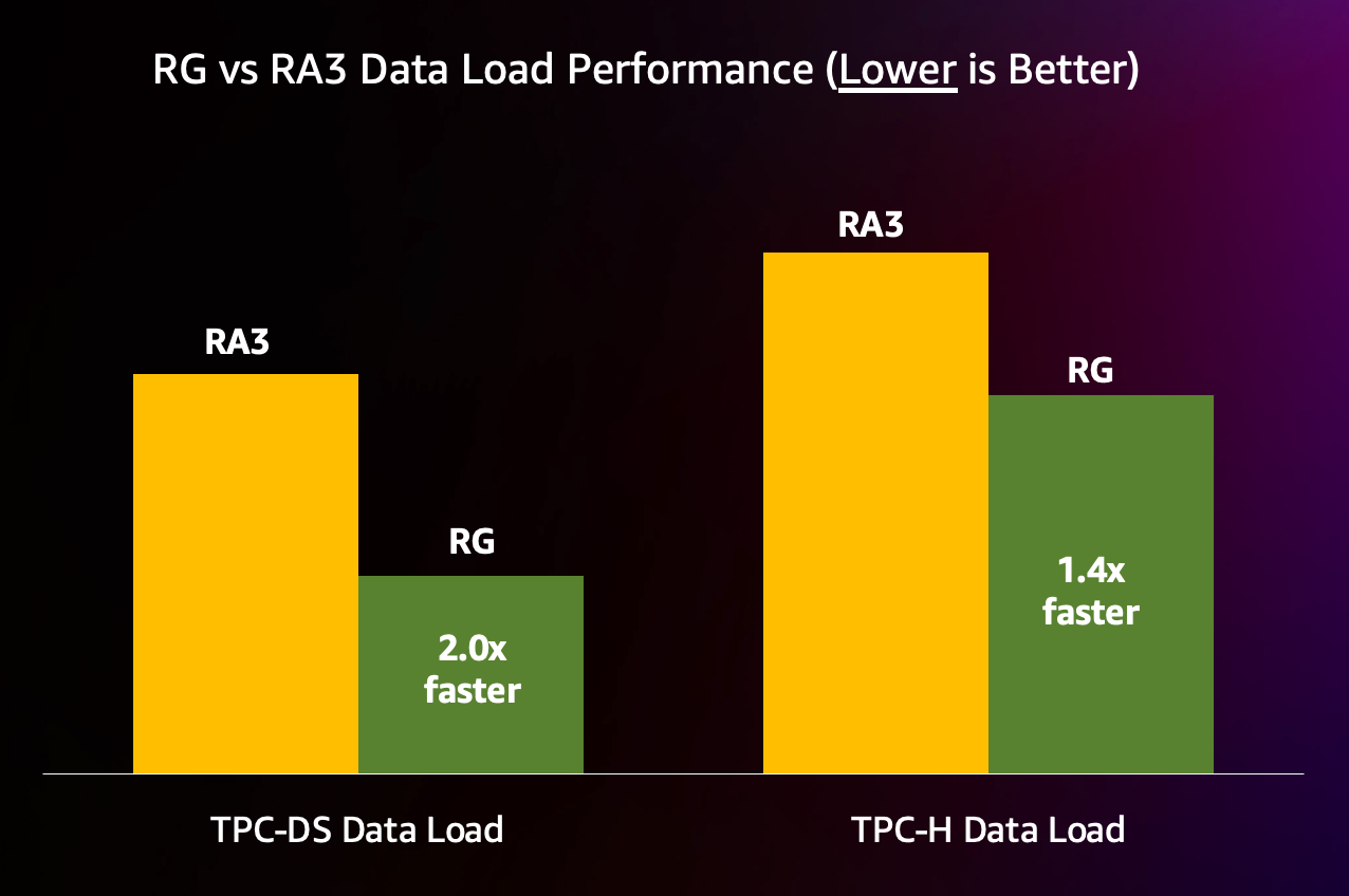
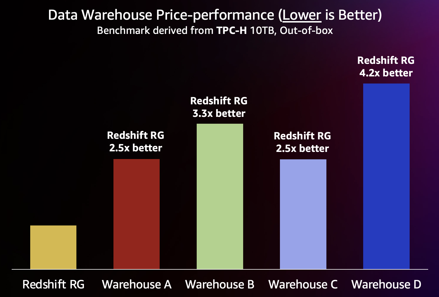
On May 12, 2026, Amazon Redshift launched Graviton-based RG instances, a new generation of provisioned nodes. RG instances deliver up to 2.2x as fast for data warehouse workloads and up to 2.4x as fast for data lake workloads, at 30 percent lower price per vCPU compared to RA3 instances. RG instances support all data lake formats supported by RA3 and remove the per-TB scanning charges for Amazon Redshift Spectrum.

In this post, you learn how to migrate Amazon Redshift RA3 clusters to Graviton-based RG instances. We compare the Elastic Resize, Classic Resize, and Snapshot/Restore migration strategies, with key considerations and best practices to support a smooth migration. We also provide mapping guidance from RA3 to RG to help you right-size your cluster.

Who should migrate to RG?

We recommend that all RA3 customers plan their migration to RG to maximize price-performance. RG is designed to deliver improved performance for both compute-intensive and I/O-intensive workloads compared to RA3, so regardless of your workload pattern, you might see performance improvements. Amazon Redshift Graviton RG instances maintain feature parity with prior-generation RA3 instances, so you can migrate without loss of functionality.
RG node types

The RG instance family currently has two node types available. The following table shows the RG instance types, hardware specifications, and the equivalent RA3 node types. Use these specifications to inform sizing decisions when migrating from RA3.

Node type Configuration vCPU Memory Max storage/node Node range Status RA3 equivalent
RG.xlarge Multi Node 4 32 GB 16 TB 2-32 GA (05/12/2026) Direct equivalent to RA3.xlplus.
RG.4xlarge Multi Node Only 16 128 GB 128 TB 2-64 GA (05/12/2026) 1.33x more vCPUs and memory vs RA3.4xlarge

Note: We plan to extend support for additional instance types in the future to provide an optimal price/performance fit for your Amazon Redshift workloads.

For more details on instance types, see the Amazon Redshift documentation.

RA3 to RG node mapping

Current Node Type Node Range Recommended RG Type Recommended RG Node Count
RA3.xlplus 1-32 RG.xlarge 1:1 mapping (same #node count)
RA3.4xlarge 2 RG.4xlarge 2 RG.4xl nodes for 2 nodes of RA3.4xl
RA3.4xlarge 3-64 RG.4xlarge 3 RG nodes per 4 RA3.4xl nodes (round up to nearest even)

Note: These are starting recommendations. Depending on your specific workloads, you might need to adjust the target RG node configurations. We recommend testing your workload in a lower environment and validating performance before committing to a target configuration. To test a full production workload, you can also use the Amazon Redshift Test Drive utility.

Mapping consideration: Within the RG family, 1 node of RG.4xlarge equals 4 nodes of RG.xlarge.

Choosing between RG node types: When sizing your Amazon Redshift cluster, a key decision is whether to use fewer large nodes or a greater number of smaller nodes. The key differentiator between RG node types is local SSD cache capacity. Larger nodes provide more local cache per node, which reduces the need to fetch data from managed storage and improves performance for I/O-intensive queries.

Consider larger node types when your workload involves:

  • Significant disk spill – complex queries with large intermediate result sets that exceed available memory.
  • Leader node-heavy processing – high numbers of concurrent client connections, complex query compilation with many joins and subqueries, or heavy final-stage aggregation.
  • Large volumes of frequently accessed data – hot datasets that benefit from local SSD cache to minimize fetches from managed storage.
  • Large result sets – queries returning substantial data volumes back to the client application.
  • Frequent metadata operations – workloads with high catalog lookup activity or CURSOR-based fetches with many small batches.

Prerequisites

You must have the following prerequisites to follow along with this post.

  • An existing Amazon Redshift cluster running RA3 node types.
  • AWS Identity and Access Management (IAM) permissions to perform resize operations (redshift:ResizeCluster, redshift:DescribeClusters).
  • AWS Command Line Interface (AWS CLI) installed and configured (for AWS CLI-based migration).
  • A recent manual snapshot (no more than 10 hours old) if you plan to use Classic Resize.
  • Sufficient storage capacity in the target RG configuration for your existing data.

Migration approach

The following diagram compares the three migration approaches.

Three migration approaches: Elastic Resize, Classic Resize, and Snapshot/Restore, showing trade-offs in downtime, write availability, and supported target configurations

Elastic Resize is the recommended method for performing the node upgrade when the target RG node configuration falls within the supported bounds of Elastic Resize. You can use it to change the node type (for example, from RA3 to RG) and to add or remove nodes from an Amazon Redshift cluster.

When an Elastic Resize is performed, Amazon Redshift first creates a snapshot of the source cluster. A new target cluster is provisioned with the latest data from the snapshot, and data is transferred to the new cluster in the background. During this period, data is read-only. When the resize nears completion, Amazon Redshift updates the endpoint to point to the new cluster and drops all connections to the source cluster. Although unlikely, in case of a failure, rollback happens automatically in most cases without manual intervention.

Advantages

  1. Typically completes quickly, taking approximately 10–15 minutes on average. We recommend it as your first option.
  2. Minimal downtime, because the cluster remains in a read-only state during the resize operation.
  3. Cluster endpoint remains the same, so no connection string changes are required.
  4. Can be run on demand or scheduled during a maintenance window.

Considerations

  1. When performing an Elastic Resize to change the node type on a producer cluster, data sharing is unavailable while connections are dropped and transferred to the new target cluster.
  2. Verify that your target node configuration has enough storage for your existing data.
  3. Not all target configurations are available under Elastic Resize. Consider Classic Resize or Snapshot/Restore in those cases.
  4. An Elastic Resize operation can’t be canceled after it’s initiated.
  5. Data slices remain unchanged. This can potentially cause some data or CPU skew.

You can use either the AWS Management Console or the AWS CLI to initiate an Elastic Resize.

To resize a cluster using the console, follow these steps

  1. Sign in to the AWS Management Console.
  2. Open the Amazon Redshift console at https://console.aws.amazon.com/redshiftv2/.
  3. On the left navigation menu, choose Provisioned clusters.
  4. Choose the cluster to resize.
  5. For Actions, choose Resize. The Resize cluster page appears.
  6. On the Resize cluster page, select the resize type: Elastic resize (recommended).Resize cluster console showing Elastic resize selected as the resize type
  7. Under New configuration, select the node type (for example, rg.4xlarge).
  8. Enter the number of nodes.
  9. Depending on your choices, choose Resize now or Schedule resize.

To resize a cluster using the AWS CLI, follow these steps

# Initiate an Elastic Resize to upgrade from RA3 to RG node type
aws redshift resize-cluster \
    --cluster-identifier <my-RA3-cluster> \  # Source cluster ID
    --node-type rg.4xlarge \                 # Target RG node type
    --number-of-nodes <#nodes> \             # Target node count
    --no-classic                            # false = Elastic Resize

2. Classic Resize

Classic Resize is recommended when the change in cluster size or node type isn’t supported by Elastic Resize. It’s also required for single-node to multi-node conversions.

When you perform a Classic Resize, Amazon Redshift creates a target cluster and migrates your data and metadata from the source cluster using a backup and restore operation. This makes sure that all data, including database schemas and user configurations, is accurately transferred. The source cluster restarts initially and is unavailable for a few minutes. After that, the cluster becomes available for read and write operations while the resize continues in the background.

Enhanced Classic Resize comprises two stages:

  1. Stage 1 (critical path): Migrating the metadata from the source cluster to the target cluster. During this stage, the source cluster is in read-only mode. This is typically a very short duration. The cluster is then made available for read and write queries. All tables with KEY distribution style are temporarily stored with EVEN distribution and are redistributed to KEY style in Stage 2.
  2. Stage 2 (off critical path): Redistributing the data per the previous distribution style. This runs in the background. Duration depends on data volume, cluster workload, and node type.

For additional details, see Accelerate resizing of Amazon Redshift clusters with enhancements to classic resize.

Advantages

  1. Supports all possible target node configurations.
  2. Allows for comprehensive reconfiguration of the source cluster.
  3. Rebalances data slices to the default per node, which leads to even data distribution across nodes.

Considerations

  1. The size of the data on the source cluster must be below 2 petabytes (PB). Use the Snapshot/Restore approach for data larger than 2 PB.
  2. Before initiating, make sure a manual snapshot is available that is no more than 10 hours old. If not, take a new manual snapshot.
  3. The snapshot used to perform the Classic Resize can’t be used for a table restore or other purpose.
  4. The cluster must be in a virtual private cloud (VPC).
  5. While the resize is in progress, queries can take longer to complete. Consider enabling concurrency scaling.
  6. Drop tables that aren’t needed before performing a Classic Resize to accelerate data distribution.
  7. Classic Resize takes more time to complete than Elastic Resize.
  8. Plan and schedule the resize operation during off-peak hours or maintenance windows.

You can use either the console or the following AWS CLI command to initiate a Classic Resize.

To run a Classic Resize through the console, follow the resize instructions in the preceding section and choose Classic resize, as shown in the following screenshot.

Resize cluster console showing Classic resize selected as the resize type

Classic Resize using the AWS CLI

# Initiate Classic Resize via AWS CLI
aws redshift resize-cluster \
    --cluster-identifier <my-ra3-cluster> \  # Source cluster ID
    --node-type rg.4xlarge \                 # Target RG node type
    --number-of-nodes <#nodes> \             # Target node count
    --classic                                # true = Classic Resize

To monitor a Classic Resize of a provisioned cluster in progress, including KEY distribution, use SYS_RESTORE_STATE. It shows the percentage completed for the table being converted. You must be a superuser to access the data.

Elastic Resize vs. Classic Resize

Behavior Elastic Resize Classic Resize
System tables Elastic Resize retains system log data. Classic Resize doesn’t retain system tables and data.
Changing node types When the node type doesn’t change, Elastic Resize is an in-place resize and most queries are held. With a new node type selected, a new cluster is created and queries are dropped as the resize completes. A new cluster is created. Queries are dropped during the resize.
Session and query retention Elastic Resize retains sessions and queries when the node type is the same in the source and target. If you choose a new node type, queries are dropped. Classic Resize doesn’t retain sessions and queries. Queries are dropped, and you can expect some performance degradation. Run the resize during a period of light use.
Canceling a resize operation You can’t cancel an Elastic Resize. For a Classic Resize to an RG or RA3 cluster, you can’t cancel.

3. Snapshot, Restore, Resize

Use this method when you need near-constant write access during the migration, or when you want to validate the new RG setup without affecting the existing cluster.

Steps

  1. In the Amazon Redshift console, choose Provisioned clusters dashboard, select your source cluster, choose Actions, then choose Create manual snapshot. Specify a snapshot name and choose Create snapshot.
  2. Select your snapshot.
  3. Choose Restore from snapshot.
  4. Specify the cluster ID and configuration (target cluster).
  5. Verify that the sample data exists in the target cluster by following these steps:
    1. Connect to the target cluster using the new endpoint.
    2. Run SELECT COUNT(*) FROM <table_name> for key tables and compare counts with the source cluster.
    3. Verify that all schemas exist.
    4. Validate that user permissions were restored correctly.
  6. If you write data to the source cluster after taking the snapshot, manually copy the data to the target cluster.
  7. Update your application connection strings to use the new cluster endpoint.

Advantages

  1. Allows validation of the new RG setup without affecting the existing cluster.
  2. Offers flexibility to restore to different Regions or Availability Zones, which provides additional disaster recovery options.
  3. Minimizes the amount of time that the cluster is unavailable for write operations.

Considerations

  1. Setting up the new cluster and restoring data can take longer than Elastic Resize.
  2. Any data written to the source cluster after the snapshot must be copied manually to the target cluster.
  3. A new Amazon Redshift endpoint is created, so connection string changes are required.
  4. To keep the cluster endpoint the same, consider renaming both clusters so the new target cluster has the same name as the original source cluster.

Fallback

You can revert to RA3 at any time using any of the migration approaches described earlier.

DMS, Zero-ETL, and data sharing considerations during migration

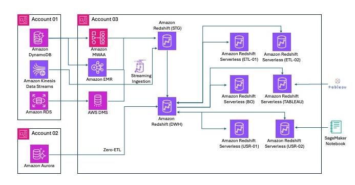
If your Amazon Redshift cluster is an AWS Database Migration Service (AWS DMS) target, has Zero-ETL integrations, or is a data sharing producer, keep the following in mind when resizing from RA3 to RG.

AWS DMS change data capture (CDC) tasks aren’t impacted by the resize. The replication instance operates independently and resumes writing after the cluster is available. No task restart is required.

Zero-ETL tables temporarily become unavailable during the resize and enter a resync state. How long the resync takes depends on data volume. Use svv_integration_table_state to check when all tables are back to Synced. For additional details, see Zero-ETL considerations.

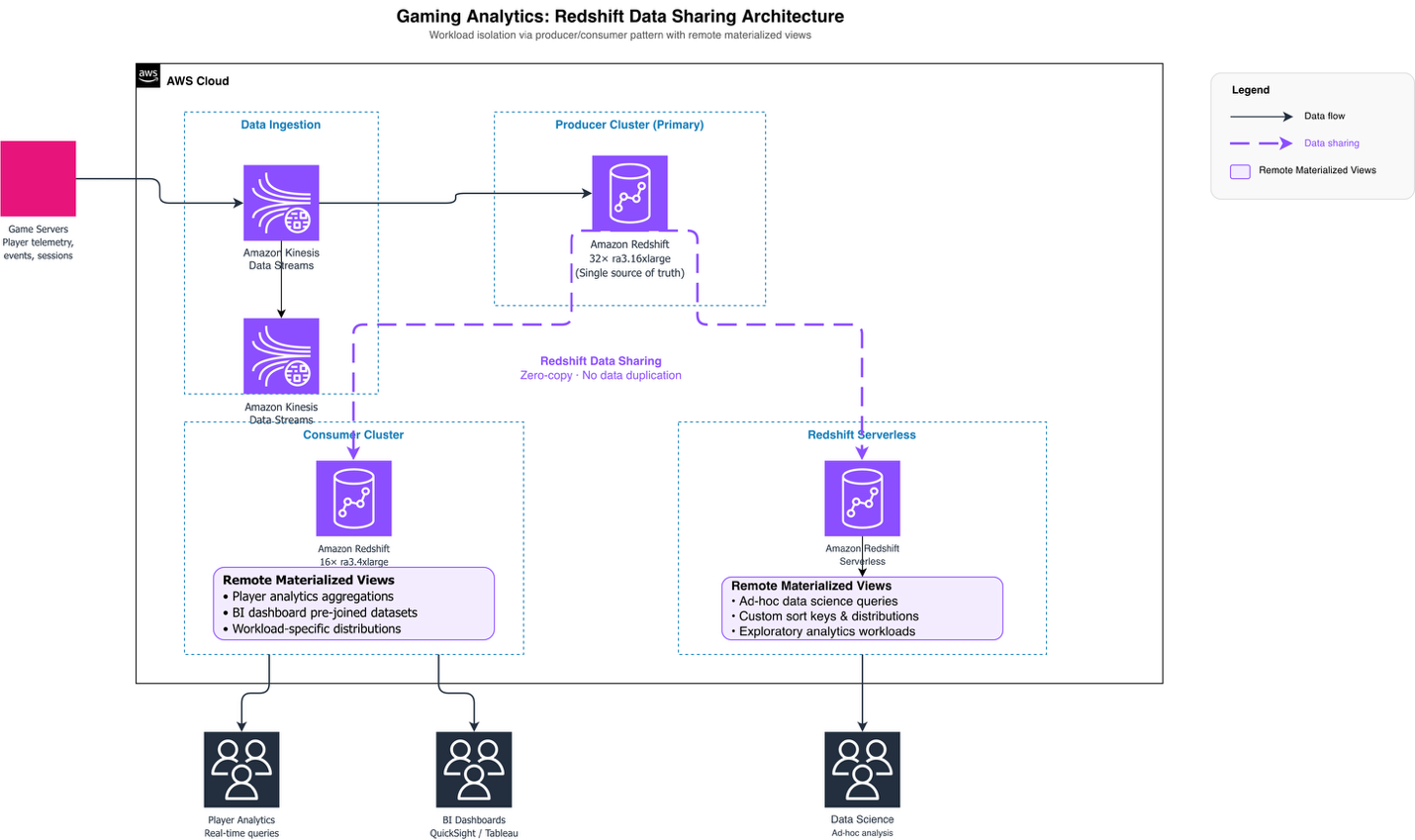
When you resize a producer cluster, data sharing is temporarily unavailable while connections transfer to the new cluster. This typically lasts several minutes. Consumer clusters can’t access shared data during this period. After the resize completes, data sharing resumes automatically with no reconfiguration needed. Plan a brief outage window for consumer workloads that depend on the producer being resized.

Snapshot/Restore impact on DMS, Zero-ETL, and data sharing

Zero-ETL integrations are tied to the original cluster. A restored cluster is treated as a new cluster, so replication doesn’t automatically resume. After the restore, you need to create a new Zero-ETL integration pointing to the restored cluster. It performs an initial sync to bring the data current.

AWS DMS connections are endpoint-based. A restored cluster receives a new endpoint, so AWS DMS tasks won’t automatically connect to it. After the restore, you must update the AWS DMS endpoint configuration with the new cluster address and restart the migration tasks.

Data sharing is tied to the cluster namespace. A restored cluster has a different namespace, so existing data shares don’t carry over. As a producer, you need to create new data shares and re-share them with consumer clusters. As a consumer, you lose access until the producer reestablishes the share from the new cluster.

Migration best practices

  1. Inform downstream teams before the migration. This includes data sharing consumers, Zero-ETL applications, and BI/ETL pipelines.
  2. Schedule the migration during a maintenance window to reduce impact on production.
  3. Take a manual snapshot before starting the resize. This serves as your rollback point.
  4. Test your target RG configuration with a representative workload before migrating production.
  5. Confirm that downstream applications are working after completion.

Clean up

To avoid incurring future charges, delete the RG provisioned cluster and any manual snapshots created during migration testing. Deleting a cluster permanently removes all data. Make sure you are deleting only the test cluster. Consider taking a final snapshot before deletion if you need to retain any test data.

Conclusion

In this post, we covered the migration options, considerations, and best practices for upgrading Amazon Redshift RA3 instances to Graviton-based RG instances. For more details on the performance benefits of RG, see the announcement blog post.

Start upgrading to Amazon Redshift RG instances today and take advantage of better price-performance with the guidance in this post. For architectural support or proof of concept (POC) assistance, contact AWS Support.


About the authors

Nita Shah

Nita Shah

Nita is a Sr. Analytics Specialist Solutions Architect at AWS based out of New York. She has been building enterprise data platforms, data warehousing, and analytics solutions for over 20 years and specializes in Amazon Redshift. She is focused on helping customers design and build enterprise-scale well-architected analytics and decision support platforms.

Ankit Sahu

Ankit brings over 18 years of expertise in building innovative data products and services. His diverse experience spans product strategy, go-to-market execution, and digital transformation initiatives. Currently, as Sr. Product Manager at Amazon Web Services (AWS), Ankit is driving the vision and strategy for Amazon Redshift.

Vinayaka Gangadhar

Vinayaka is an Analytics Specialist at Amazon Web Services (AWS), where he helps customers build and troubleshoot scalable data platforms and derive meaningful insights through AWS analytics services, with deep expertise in Amazon Redshift and Amazon OpenSearch. When not solving complex analytics challenges, he enjoys exploring new technologies and spending quality time with his family. LinkedIn: /vinayaka-gangadhar

Ricardo Serafim

Ricardo Serafim

Ricardo is a Senior Analytics Specialist Solutions Architect at AWS.

AWS WAF adds AI traffic monetization capability to help content owners charge AI bots for content access

Post Syndicated from Esra Kayabali original https://aws.amazon.com/blogs/aws/aws-waf-adds-ai-traffic-monetization-capability-to-help-content-owners-charge-ai-bots-for-content-access/

AWS WAF now includes AI traffic monetization capability that gives digital content owners and publishers a way to charge AI bots and agents for access to protected web content directly at the network edge. The capability helps content owners and publishers set per-request pricing by content path, bot category, or verification tier without modifying their origin infrastructure or writing application code. Content owners can define granular access policies per agent type, collect payments in stablecoins to their preferred wallet, and monitor revenue and bot activity from a single dashboard.

AI bot traffic now accounts for more than 50% of web traffic for many content providers, with AI-specific crawlers growing more than 300% year-over-year. Unlike traditional search engine crawlers, which index content and return measurable referral traffic back to publisher websites, AI bots consume the same content to generate summaries and responses in AI interfaces, with little to no traffic sent back to the original source. Publishers bear the infrastructure costs of serving that traffic without the page views, ad impressions, or subscription conversions that typically offset those costs. AWS WAF Bot Control already gives customers visibility into bot activity and the ability to block or rate-limit traffic, but setting pricing and collecting payment from AI agents has not been possible until now. AI traffic monetization is a new Bot Control capability that closes that gap, giving content owners and publishers a way to configure pricing rules directly through the AWS WAF console and collect payments from AI agents through third-party payment integrations, without building custom payment infrastructure or negotiating individual licensing agreements. Payment settlement and verification flows are provided by Coinbase’s x402 Facilitator. Integration with Stripe for direct account payments and Machine Payments Protocol (MPP) support is coming soon.
Getting Started with AI Traffic Monetization
Before configuring monetization, confirm that AWS WAF Bot Control is enabled at Common or Targeted level on the web ACL associated with your CloudFront distribution. Bot Control provides the agent classification that monetization rules depend on. If you have not set this up yet, visit Adding the AWS WAF Bot Control managed rule group to your web ACL documentation. In the AWS Management Console, go to WAF & Shield and choose Protection packs (web ACLs) in the left navigation pane to get started.

A protection pack is the core configuration unit for AI traffic monetization. It defines which content paths are monetized, what each agent verification tier is charged, which payment methods you accept, and what license terms apply. To create one, choose Create protection pack (web ACL).

In Tell us about your app, select one or more app categories that describe your content (for example, Content & publishing systems, E-commerce & transaction platforms, or Enterprise & business applications), and choose an App focus. AWS WAF uses these selections to recommend suitable security protections for your configuration.

In Select resources to protect, choose Add resources to associate regional or global resources such as CloudFront distributions with this protection pack. You can skip this step and add resources later.

In Choose initial protections, select from AWS WAF managed rule packages based on your app category and resource selections. You can also choose individual rules instead of packages.

In Name and describe, provide a name and optional description for the protection pack.

Optionally, expand Customize protection pack (web ACL) to configure additional settings including pricing tiers, payment methods, content scope, and license terms.

When finished, choose Create protection pack (web ACL).

Once your protection pack is in place, review the AI traffic analysis dashboard to understand the impact of AI bot traffic on your content before setting your pricing strategy. In the WAF & Shield console, go to AI traffic analysis in the left navigation pane. Select your protection pack (web ACL) from the dropdown to populate the dashboard.

The AI traffic analysis dashboard breaks down traffic into four categories visible in the bot traffic overview panel: All bot requests, AI bot requests, Verified AI bot traffic, and Unverified AI bot traffic. The dashboard surfaces infrastructure impact metrics including bandwidth consumed, estimated monthly cost, and peak request rates. A per-path heatmap shows which content paths receive the most AI bot activity by hour, giving you the data you need to make informed pricing decisions.

AWS WAF Bot Control classifies over 650 distinct AI bot and agent types including GPTBot, Claude-Web, and Perplexity-Bot, and assigns each a verification tier:

  • Verified — Agent identity confirmed through Web Bot Auth (WBA) Ed25519 cryptographic signature, or sourced from a documented IP range with a known set of user-agents and domain names.
  • Unverified — Agent recognized through user-agent matching, behavioral fingerprinting, and IP reputation, but identity not cryptographically confirmed.

Once you have reviewed your traffic patterns, return to Protection packs (web ACLs), select your protection pack from the list, and choose Configure AI monetization from the right panel to set pricing and access policies. Each protection pack defines the pricing, agent policies, accepted payment methods, and license terms that apply to a defined set of content paths. You can create multiple protection packs and apply different pricing to different content zones within the same distribution. Once created, associate the protection pack with your web ACL by opening the web ACL and choosing Add protection pack.

For each agent verification tier within the pack, you can assign one of six actions: Monetize (return a 402 with pricing), Allow (grant free access), Block (deny access entirely), Count (log without charging), CAPTCHA (present a puzzle to verify a human sender), or Challenge (run a silent check to verify the client is a browser, not a bot).

In the Edit monetization configuration page, configure the following:

Under Payment settlement, select one or more blockchain networks for stablecoin payments. Any wallet address on the supported networks is accepted, whether self-managed or hosted by a wallet provider such as Coinbase. For each network, provide your wallet address and set a Base price per page in USDC. You can add multiple networks using Add network. AWS does not process payments or take a fee on content revenue; disbursement is self-managed or managed by your wallet provider.
When a Monetize rule matches an incoming request, AWS WAF returns an HTTP 402 Payment Required response. The response body contains a machine-readable price manifest in JSON format using the x402 open protocol for machine-to-machine payments. The manifest includes the content price in USDC, accepted blockchain networks such as Base and Solana, the destination wallet address, the maximum payment timeout, and the payment scheme.
Any x402-compatible agent runtime can complete this flow autonomously. The client submits a signed payment authorization on their payment network of choice. AWS WAF verifies it, fetches the content, integrates with third-party facilitator services for settling the payment on-chain, and serves the response.

Note that the Monetize action is supported exclusively for web ACLs associated with Amazon CloudFront distributions. Adding a Monetize rule to a regional web ACL is not supported.

Since the Currency mode toggle is available directly in the monetization configuration page, you can switch between Real and Test mode at any time. Before going live, use test mode on non-production traffic to validate pricing, wallet configuration, and x402 payment flows. Note that test mode still enforces x402 payments, but those payments can be made on testnets such as Base Sepolia or Solana Devnet using test funds obtained from faucets such as faucet.circle.com. To activate test mode, toggle Currency mode to Test in your protection pack configuration. AWS WAF returns real price manifests and runs the full payment flow identically to production on the configured test chain. All events are logged with CurrencyMode: TEST. When satisfied with the configuration, toggle Currency mode back to Real to begin processing real payments.
Once you have switched Currency mode to Real, navigate to AI access monetization in the left navigation pane to track monetization outcomes in real time. Note that the AI access monetization dashboard only reflects activity from real currency mode and does not display test transactions.

The Revenue dashboard shows Total revenue, revenue broken down by Verified bots and Unverified bots, and Avg. per request. The Top revenue sources panel groups earnings by bot category, and the AI access patterns panel ranks content paths by revenue generated. Use the Settlements tab to reconcile payments by provider and review payment method distribution and failed payment attempts.
Now Available
AI traffic monetization is available now for Amazon CloudFront customers at no additional charge beyond standard AWS WAF pricing. The capability is available in all edge locations where AWS WAF web ACLs are associated with Amazon CloudFront distributions.
To learn more about AI traffic monetization, see the AWS WAF Developer Guide.
— Esra

AWS Weekly Roundup: AWS FinOps Agent in preview, Gemma 4 on Bedrock, Kiro Pro Max, and more (June 15, 2026)

Post Syndicated from Esra Kayabali original https://aws.amazon.com/blogs/aws/aws-weekly-roundup-aws-finops-agent-in-preview-gemma-4-on-bedrock-kiro-pro-max-and-more-june-15-2026/

This week, New York City is hosting AWS Summit, bringing together builders, customers, and AWS teams for a full day of announcements, demos, and technical sessions at the Javits Center. I wrote blog posts for some of the Summit launches, so I am excited to see them go live this week. I just won’t be watching from the Javits Center. I’ll be at a four-day music festival, following the launches on my phone while trying to figure out how to put up a tent. If you weren’t able to attend in person like me, the keynote livestream is available on June 17, with Dr. Swami Sivasubramanian, VP of Agentic AI, and Chet Kapoor, VP of Security Services and Observability, covering new capabilities across developer tools, AI infrastructure, and security.

Here’s what happened this week.

Headlines
How frontier teams are reinventing AI-native development — Swami published a detailed post this week drawing on data from experiments across hundreds of Amazon engineering teams. The findings are worth reading carefully if you are thinking about how to structure AI adoption on your own team.

A six-engineer team rebuilt the Amazon Bedrock inference engine in 76 days, a project originally scoped for 30 developers over 12 to 18 months. The median productivity gain across structured pilots with Amazon Stores teams was 4.5x in normalized deployment velocity, with some teams exceeding 10x. Perfect Order Experience went from a two-week feature cycle to shipping in an afternoon. WW Grocery cut design document creation from five days to a few hours.

The post distills these results into five practices for becoming a frontier team. First, invest in agent context: build steering files, coding standards, and structured repositories before writing production code. Second, expect an initial slowdown while workflows are restructured, and push through it. Third, maintain a steady backlog of well-scoped tasks so agents can run in parallel without constant supervision. Fourth, make intent explicit through structured specifications before code generation begins. Fifth, shift testing left so agents can self-correct before code reaches the pipeline.

The post closes with a note that commit velocity is only part of the picture, and that a follow-up will cover release management, operations, security operations, and EOL upgrades.

AWS FinOps Agent is now available in preview — AWS FinOps Agent is a new agent for FinOps practitioners and engineering teams that answers cost questions, surfaces optimization opportunities, investigates cost anomalies, and runs recurring FinOps workflows on a defined schedule. You can use it to query your AWS costs, generate cost reports for finance and engineering teams, and surface rightsizing, idle resource, and Savings Plans recommendations from AWS Cost Optimization Hub and AWS Compute Optimizer. The agent can open Jira tickets on your behalf based on those recommendations. When a cost anomaly is detected, FinOps Agent can automatically investigate the root cause and post findings to a Slack channel.

Last week’s launches
I’ll start with one I wrote this week, then cover the other launches that caught my attention:

  • Amazon EC2 M9g and M9gd instances are now generally available — Powered by AWS Graviton5 processors and built on the sixth-generation AWS Nitro System, M9g instances deliver up to 25% better compute performance compared to Graviton4-based instances, with up to 35% faster performance for web applications, up to 35% for machine learning inference, and up to 30% for databases. Graviton5 is the first processor in the AWS fleet to support PCIe Gen6 and DDR5-8800 memory, and includes a 5x larger L3 cache compared to the previous generation. M9g and M9gd instances offer up to 15% higher network bandwidth and 20% higher Amazon EBS bandwidth on average across sizes compared to M8g. This release also introduces the Nitro Isolation Engine, an enhancement to the Nitro System that uses formal verification to provide mathematically proven isolation between virtual machines — establishing Nitro as the first formally verified cloud hypervisor. M9gd instances add up to 11.4 TB of NVMe SSD local storage with 30% higher IOPS compared to M8gd. Both instance types support Instance Bandwidth Configuration (IBC) for adjusting bandwidth allocation between EBS and VPC networking by up to 25%.
  • Anthropic Claude Fable 5 on Amazon Bedrock — Claude Fable 5 launched on Amazon Bedrock on June 9, bringing extended asynchronous task execution, advanced vision capabilities across diagrams, charts, and PDFs, and proactive self-verification. Access requires opting into data sharing via the Data Retention API before invoking the model; Anthropic requires 30-day retention of inputs and outputs for Mythos-class models. Important note on availability: On June 12, Anthropic asked AWS to revoke access to Claude Fable 5 and Claude Mythos 5 for all users to support compliance with a US Government export control directive. All other models, including Opus 4.8, are unaffected. Read the Anthropic statement for details. AWS will share further updates as they become available.
  • Gemma 4 models are now available on Amazon Bedrock — The Gemma 4 family from Google DeepMind is now available on Amazon Bedrock across three variants: Gemma 4 31B (dense, 256K-token context window, suited for reasoning and coding workloads), Gemma 4 26B-A4B (mixture-of-experts architecture, targeting cost- and latency-sensitive workloads), and Gemma 4 E2B (smallest variant, designed for low-latency interactive use cases). All three support native function calling, structured output, reasoning, response streaming, multimodal input across text, image, video, and audio, and more than 35 languages.
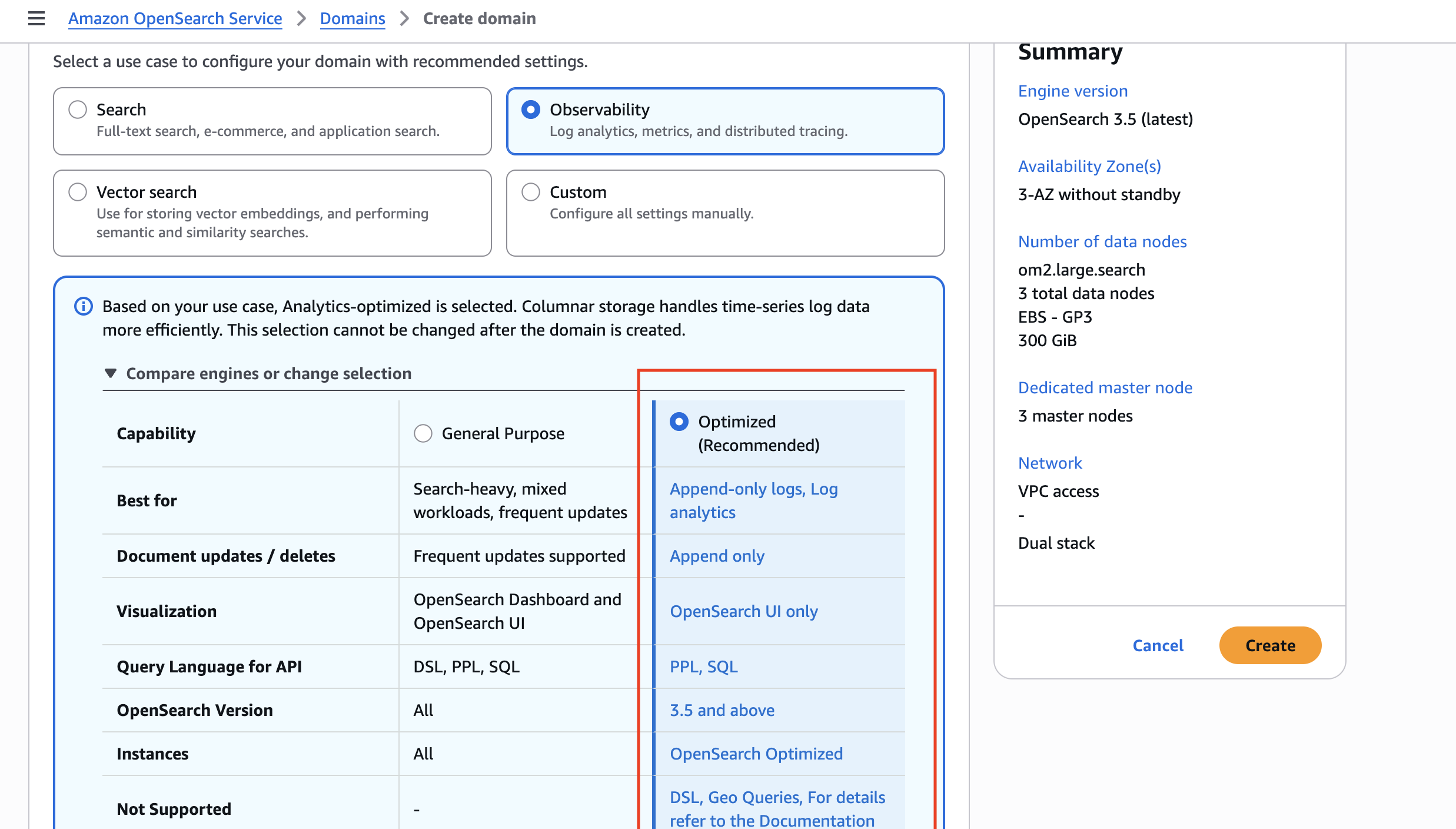
  • Amazon OpenSearch Service launches MCP Apps for agentic observability — Amazon OpenSearch Service now supports MCP Apps, enabling observability workflows inside compatible agentic IDEs including Claude Desktop and VS Code. An AI agent in your local environment can investigate incidents using logs, traces, metrics, and alerts stored in OpenSearch domains, collections, and Amazon Managed Service for Prometheus. Each MCP App tool call returns a dual response: a text summary for the agent to reason over and an interactive visualization rendered in the same conversation thread. Available MCP App tools cover log, metrics, and trace investigation; service performance; topology; dynamic visualizations; agent health; cluster health; and instrumentation scoring.

Other AWS news
Here are some additional posts and updates you may find useful:

  • AWS CLI v1 enters maintenance mode — When CLI v1 enters maintenance mode, the botocore and s3transfer dependencies will be vendored directly into the CLI v1 codebase rather than installed as separate packages. This means upgrading CLI v1 will no longer update the standalone botocore or s3transfer packages, and installing those packages independently will have no effect on the versions used by CLI v1. Environments with both CLI v1 and boto3 installed will contain separate copies of these libraries. New CLI v1 releases will be limited to critical bug fixes and security issues. The recommended path is to migrate to AWS CLI v2.
  • AWS Workload Credentials Provider is now available — AWS has launched a new Workload Credentials Provider that enables workloads to obtain short-term AWS credentials without requiring long-term access keys. This supports credential management for applications running outside of AWS, giving teams a way to follow least-privilege access patterns for workloads in third-party or on-premises environments.
  • Kiro Pro Max is now available — Kiro has introduced a new Pro Max tier, adding higher usage limits, access to the latest frontier models, and additional agentic capabilities for development teams. Kiro Pro Max is designed for professional developers who need sustained, high-volume use across coding, specification generation, and agent-driven tasks.

Upcoming AWS events
Check your calendar and sign up for upcoming AWS events:

Visit the AWS Builder Center to meet other builders, contribute solutions, and find resources that help you keep building. You can also browse upcoming AWS-led in-person and virtual events, plus developer-focused sessions.

— Esra

This post is part of our Weekly Roundup series. Check back each week for a quick roundup of interesting news and announcements from AWS!

Access Amazon S3 data files directly using AWS Lake Formation permissions

Post Syndicated from Aarthi Srinivasan original https://aws.amazon.com/blogs/big-data/access-amazon-s3-data-files-directly-using-aws-lake-formation-permissions/

Data scientists and ML engineers often need to access raw data files in Amazon Simple Storage Service (Amazon S3) for machine learning training, data exploration, and generative AI workflows. However, when table-level access is governed by AWS Lake Formation, accessing the underlying S3 files has required maintaining separate permission mechanisms. S3 bucket policies or AWS Identity and Access Management (IAM) role policies create operational overhead and risk of permission drift.

Lake Formation now supports direct access to S3 data file locations for tables whose permissions it manages. Previously, data scientists with Lake Formation permissions on AWS Glue Data Catalog tables could query them using spark.sql(). Now, they can also read and write the underlying S3 data files using spark.read.parquet() or spark.read.csv() from Amazon EMR Spark jobs, Amazon SageMaker Unified Studio notebooks with EMR compute, and custom applications. All access is governed by the same Lake Formation permissions.

This capability is powered by the new GetTemporaryDataLocationCredentials() API, which vends temporary credentials scoped to registered S3 locations when callers have appropriate Lake Formation permissions on the corresponding Data Catalog tables. This eliminates the need to manage separate S3 bucket policies for file-level access while maintaining fine-grained access control in Lake Formation for table-based access. It enables your data scientists to explore S3 datasets securely, accelerate machine learning pipelines, and build generative AI workflows without compromising governance.

In this post, we demonstrate reading from and writing to Lake Formation-managed S3 locations using Apache Spark jobs from EMR. Lake Formation credential vending for S3 location access is available in EMR release label 7.13 and later, Boto3 1.42.29 and later, AWS Java SDK 2.41.32 and later, and AWS Command Line Interface (AWS CLI) version 2.33.1 and later.

Key use cases for Lake Formation permissions to S3 locations

  • Unified permissions for Analytics and Machine Learning pipelines – Data scientists can access both structured tables through SQL queries and underlying data files through programmatic APIs for machine learning and AI workloads. They are empowered to use tools of their choice – for example, use Amazon Athena for SQL analytics with the table names while read and write to the underlying files in their SageMaker notebook or Spark application with spark.read.parquet(“s3://bucket/database_path/table_files/).
  • Enable AI ready data lakes – Machine learning pipelines can read training data directly from governed data lakes. Generative AI applications can access foundation model training datasets, and data exploration workflows to use native file APIs while maintaining centralized governance and compliance.
  • Reduced operational complexity – Operations teams don’t need to maintain separate permission policies – one in Lake Formation for table access and another in S3 bucket policies or AWS Identity and Access Management (IAM) roles for file access. This reduces the risk of permission mismatches and avoids inconsistent access control.
  • Unified audit capability – Auditors do not need to examine multiple log sources, such as S3 Access Logs, AWS CloudTrail events from different services, to understand who accessed what data and when. With this feature, you get a unified CloudTrail audit trail showing both table access through SQL engines and file access through direct APIs, with each access event linked to the Lake Formation permission grant.

What customers are saying

“Through our close collaboration with AWS, Lake Formation’s new S3 location-based permissions have transformed how we manage data governance at Intuit. By unifying two separate access mechanisms for the same data into one unified permission model, we’ve dramatically reduced complexity and streamlined our auditing process. This is exactly the kind of simplification that lets our teams move faster without compromising security, ensuring we maintain the strict compliance and governance standards our regulators expect.”

— Tapan Upadhyay, Group Engineering Manager, Intuit

Lake Formation Credential Vending Plugin for AWS SDK v2 for Java

Lake Formation has made available a specialized library AWS Lake Formation Credential Vending Plugin for AWS SDK V2 for Java. The Java plugin intercepts S3 requests for data, checks Lake Formation permissions for the requested location, and provides temporary scoped credentials to the client if permissions are granted in Lake Formation. If the S3 location access permissions are not managed by Lake Formation, the plugin checks for access in Amazon S3 Access Grants and lastly falls back to IAM permissions. The plugin is supported independently of Spark and comes as an enhancement to EMR Spark Full Table Access (FTA) mode, starting in EMR 7.13 and later. The plugin is integrated at the S3A level. Therefore, any client of S3A can enable it by setting the S3A configurations, in addition to the EMR Lake Formation Full Table Access (FTA) configuration as follows:

fs.s3a.lakeformation.access.grants.enabled = true
fs.s3a.lakeformation.access.grants.fallback.to.iam = true

With the Java plugin, you can enable governance for data lake resources in your custom applications with Lake Formation permissions – managing both fine grained access for users requiring restricted access on Data Catalog tables while providing direct S3 object level access to use-cases that require them.

Note: (1) The principal that will be accessing direct S3 locations of the tables will require full table access. That is, Lake Formation SELECT permission on all columns and rows of the table is required. (2) The Spark cluster needs FTA configuration. (3) Currently, Apache Iceberg table format is not supported with this plugin.

Solution overview

A financial services company runs daily ETL jobs using Spark in EMR. They process raw transaction records in S3 and store the processed records in another S3 location. The transformed Parquet data is registered with Lake Formation and cataloged as a table in Data Catalog. The ETL job will have direct IAM access to the raw data location, while it uses Lake Formation permissions to write to and read from the curated table location. Downstream, a data-analyst role will query the curated table, with restricted column access. The solution is shown in Figure 1.

Figure 1 – Architecture shows EMR Spark writing curated records to the S3 location of a table using Lake Formation permissions while Data-Analyst queries the same table with Lake Formation fine grained access control in Athena.

Architecture diagram showing EMR Spark writing curated records to the S3 location of a table using Lake Formation permissions while Data-Analyst queries the same table with Lake Formation fine-grained access control in Athena

Prerequisites

To get started exploring this feature, we recommend you have the following setup.

Solution walkthrough

First, we will get the setup ready with S3, sample database, table, and data. We will add a raw data set to S3 location, create a table with parquet data in another S3 location that represents the curated dataset for further downstream consumption. We will register the table data location with Lake Formation and grant permissions for the EMR run time role and Data-Analyst role.

Your S3 bucket will have the following structure.

Raw data – s3://<your-bucket-name>/raw/transactions/dt=2024-03-21/

Process data for table – s3://<your-bucket-name>/processed/transactions/

Spark script – s3://<your-bucket-name>/scripts/

Logs for the EMR cluster – s3://<your-bucket-name>/logs/

Step 1 – Create a parquet table in Data Catalog

From the Athena console query editor, create a table in Data Catalog.

-- Create a database
CREATE DATABASE finance_db;

-- Create an external table pointing to the S3 location
CREATE EXTERNAL TABLE IF NOT EXISTS finance_db.transactions_processed (
    transaction_id STRING,
    merchant_name STRING,
    amount DECIMAL(18,2),
    currency STRING,
    account_number STRING,
    card_type STRING,
    status STRING,
    region STRING
)
PARTITIONED BY (transaction_date DATE)
STORED AS PARQUET
LOCATION 's3:///processed/transactions/'
TBLPROPERTIES (
    'parquet.compress'='SNAPPY'
);

Step 2 – Register S3 location and grant table permission to IAM roles in Lake Formation

2.1 Register the table data location s3://<your-bucket-name>/processed/transactions/ with Lake Formation in Lake Formation mode using the custom S3 registration IAM role. For details on how to register locations with Lake Formation, refer Adding an Amazon S3 location to your data lake.

2.2 Grant DESCRIBE permission on the database finance_db and ALL permission on the table transactions_processed to your EMR runtime role.

2.3 Grant Data location permission to EMR runtime role on the curated table’s location. This is to allow writing to that location.

2.4 Grant DESCRIBE permission on the database finance_db and SELECT permission on the table transactions_processed to your Data-Analyst role. Exclude the columns transaction_id and account_number while granting SELECT permissions on the table to the Data-Analyst role.

For details on how to grant Lake Formation permissions, refer Granting database permissions using the named resource method; Granting table permissions using the named resource method and Granting data location permissions.

Step 3 – Run ETL script in EMR

3.1 Download the script bdb-5860-script.py.

3.2 Edit the S3 bucket name placeholder in the script (RAW_PATH and TABLE_PATH) to your resource names and upload to your S3 path s3://<your-bucket-name>/scripts/.

3.3 Make sure your EMR runtime role has access to the script location in its IAM policy permissions.

3.4 Submit and run the script as a step to the EMR cluster, following instructions at Add a Spark step.

What does the script do?

It populates raw records of transaction data into a Spark data frame, writes to the raw data bucket location using IAM permissions on the EMR runtime role. We apply some transformations and write directly to the S3 location of the table that is registered with Lake Formation, from the data frame using Spark’s native Parquet writer.

The following figure shows the stdout of the step.

EMR step stdout showing successful Spark job execution with data written to the Lake Formation-managed S3 location

The Java plugin integrated into EMR 7.13 automatically handles the access for the table’s data location registered with Lake Formation, so you don’t need to manually call the GetTemporaryDataLocationCredentials() API. In this example, the table data location s3://<your-bucket-name>/processed/transactions/ is registered with Lake Formation, for which EMR runtime role is granted ALL permissions. The direct S3 location access support by Lake Formation allows reading and writing to the location directly using Spark data frame.

Step 4 – Run query as Data-Analyst using Athena

Log in as the Data-Analyst role to the Athena console. Run a select query on the table as follows.

SELECT * FROM finance_db.transactions_processed WHERE status = 'DECLINED' AND transaction_date=DATE '2024-03-21';

The Data-Analyst role should see all but two columns of the table.

Athena query results showing the Data-Analyst role can access all columns except transaction_id and account_number

With these steps complete, we’ve read from and written to direct S3 locations using Spark data frames with the syntax s3://bucketname/prefix/, and accessed the same data using database_name.table_name syntax with Lake Formation permissions. This shows fine-grained access at table level and coarse-grained access at the file path level.

Clean up

To avoid incurring costs, clean up the resources you created for this post.

  1. Delete the Data Catalog database and tables. This removes the related Lake Formation permissions too. Remove the S3 bucket registration from Lake Formation.
  2. Delete the data files, logs, and the PySpark script of this post from your S3 bucket.
  3. Terminate the EMR cluster.

Conclusion

In this post, we showed how to use Lake Formation’s direct S3 location access to read and write data files using Spark data frames from Amazon EMR, while maintaining unified governance through Lake Formation permissions. We walked through the GetTemporaryDataLocationCredentials() API and the AWS Lake Formation Credential Vending Plugin for AWS SDK v2 for Java, which is integrated into EMR release labels 7.13 and later.

This capability unifies permission management for both fine-grained table-based access and direct S3 file path access in Lake Formation. Your data scientists can now use spark.read.parquet() and spark.write alongside spark.sql(), governed by the same permissions, audited in the same CloudTrail logs, and managed from a single console.

To get started, launch an EMR 7.13 cluster and start exploring the feature. Here are some additional resources:

Acknowledgements: We would like to thank all the team members who worked to launch this feature successfully – Rajas Bhate, Akhil Yendluri, Kunal Parikh, Sharda Khubchandani, Dhananjay Badaya, Santhosh Padmanabhan, Nitin Agrawal and Sandeep Adwankar.


About the authors

Aarthi Srinivasan

Aarthi Srinivasan

Aarthi is a Senior Big Data Architect at Amazon Web Services (AWS). She works with AWS customers and partners to architect data lake solutions, enhance product features, and establish best practices for data governance.

Archana Inapudi

Archana Inapudi

Archana is a Senior Solutions Architect at Amazon Web Services (AWS). She works with strategic enterprise customers to drive cloud data modernization, architect data lake and analytics solutions, and establish best practices for data governance and security. With over 15 years of experience in cloud, data engineering, and AI/ML, Archana is passionate about using technology to accelerate growth and deliver business outcomes.

Srinivasan Krishnasamy

Srinivasan Krishnasamy

Srinivasan is a Principal Delivery Consultant at AWS with 25+ years of experience architecting data and analytics solutions at scale. He partners with enterprise customers to modernize data platforms, build robust data governance frameworks, and drive measurable business outcomes on AWS, using the full spectrum of data engineering, AI/ML, and generative AI. Outside of work, he enjoys hiking, swimming, and gardening.

Anandkumar Kaliaperumal

Anandkumar Kaliaperumal

Anandkumar is a Senior Delivery Consultant at AWS, bringing over 23 years of deep expertise in data and analytics. A specialist in architecting scalable data analytics, AI/ML, and generative AI solutions, he thrives on tackling complex data challenges spanning data engineering, analytics, machine learning, and generative AI workloads.

Mitali Sheth

Mitali Sheth

Mitali is a Streaming Data Engineer at Amazon Web Services (AWS) Professional Services. She works with strategic software customers to architect real-time analytics solutions, design event-driven architectures, and modernize streaming infrastructure using Amazon MSK, Amazon Managed Flink, AWS Glue, and AWS Lake Formation. She holds an M.S. in Computer Science from the University of Florida.

Introducing the Snowflake and AWS Custom Lens for the AWS Well-Architected Framework

Post Syndicated from Nidhi Gupta original https://aws.amazon.com/blogs/architecture/introducing-the-snowflake-and-aws-custom-lens-for-the-aws-well-architected-framework/

Running Snowflake on AWS means navigating two distinct sets of best practices simultaneously: AWS Well-Architected guidance for infrastructure, and Snowflake Well-Architected Framework guidance for compute, data organization, and governance. Without a unified review framework, security controls go unmapped to Snowflake configurations. Production readiness timelines stretch as teams reconcile guidance from two separate review processes, and compliance posture becomes difficult to demonstrate when audit evidence spans disconnected sources. The Snowflake and AWS Custom Well-Architected Framework Lens closes that gap.

The lens brings together AWS Well-Architected best practices and Snowflake guidance into a single review experience, with integrated recommendations that reflect how the two services compose in production. It evaluates your architecture across the seven AWS Well-Architected pillars: security, reliability, performance efficiency, cost optimization, operational excellence, and sustainability. A single review surfaces findings like misconfigured Snowflake network policies alongside Amazon Virtual Private Cloud (Amazon VPC) controls, or cost inefficiencies that span both Snowflake virtual warehouse sizing and Amazon Elastic Compute Cloud (Amazon EC2) instance selection. In this post, we walk through each pillar, the three access points (AWS Management Console, Kiro, and Snowflake Cortex Code), and how to run your first review.

What’s in the lens?

The Snowflake and AWS Custom WAF Lens defines seven pillars for joint Snowflake-on-AWS architectures, drawing from both the seven-pillar AWS Well-Architected Framework and the five-pillar Snowflake Well-Architected Framework.

Pillar 1: Security and identity

Security for Snowflake on AWS requires coordinated identity and access controls across two distinct planes. On the AWS infrastructure side, services like AWS Key Management Service (AWS KMS), AWS IAM Identity Center, and Amazon VPC configurations govern access and encryption. On the Snowflake side, network policies, role-based access control (RBAC) hierarchies, and OAuth or key pair authentication control who can access data. The following table maps the most critical security domains (identity, network, authentication, and authorization) across both services, with integrated recommendations for where the two layers must align to help prevent unauthorized access.

Domain AWS guidance Snowflake guidance Integrated recommendation
Network security Amazon VPC design, AWS PrivateLink endpoints, AWS service endpoints, Amazon EC2 security groups Network policies, IP allow lists Use AWS PrivateLink between Amazon VPC and Snowflake; layer Snowflake network policies on top of EC2 security groups for defense-in-depth
Identity and access AWS Identity and Access Management (IAM) roles, federation, least privilege Database roles, role hierarchy, MFA Federate Snowflake authentication through AWS IAM Identity Center; map identity provider groups to Snowflake database roles for consistent RBAC
Authentication MFA for human IAM users; integrate with corporate IdP via IAM Identity Center RSA key pair for service accounts; SAML SSO or OAuth for humans; disable-password only Store private keys in AWS Secrets Manager; rotate via automation; unified IdP for both systems via SAML federation
Authorization Service control policies at organization level as hard guardrails; permission boundaries on delegated roles Role hierarchy with inheritance; SECURITYADMIN for grants separate for SYSADMIN Map AWS IAM roles 1:1 to Snowflake functional roles with workload identity federation

Pillar 2: Data governance and compliance

Protecting data itself, independent of who accesses it, spans two complementary layers. On the AWS infrastructure side, services like AWS KMS, AWS IAM Identity Center, and Amazon Simple Storage Service (Amazon S3) lifecycle policies govern encryption, classification, and retention of data at rest. On the Snowflake side, dynamic data masking, row access policies, Tri-Secret Secure, and automatic classification protect sensitive data at the query layer. The following table maps the most critical governance domains (classification, dynamic data masking, lineage, retention, and compliance) across both systems, with integrated recommendations for maintaining consistent data protection end-to-end.

Domain AWS guidance Snowflake guidance Integrated recommendation
Data protection AWS KMS customer-managed keys, Amazon S3 encryption Dynamic masking, row access policies, Tri-Secret Secure Use AWS KMS with Snowflake Tri-Secret Secure for dual-custody encryption; apply Snowflake masking policies for column-level protection
Audit and compliance AWS CloudTrail, AWS Config, AWS Security Hub Event tables, Account Usage, Access History, Sensitive data classification Stream Snowflake audit logs to Amazon CloudWatch or Amazon OpenSearch Service using Amazon S3 and Amazon EventBridge for consolidated compliance monitoring. AWS provides compliance-enabling capabilities; your team uses them to support and demonstrate compliance.
Row access policies AWS Lake Formation row-level filters, Amazon S3 Access Points for team-scoped access Row access policies for multi-tenant isolation or regional data residency; role-based row visibility Define row-level security once in Snowflake (single enforcement point); restrict AWS-side to pipeline service account

Pillar 3: Reliability

Reliability in a Snowflake on AWS architecture depends on how well the two systems coordinate during failure scenarios, from AWS infrastructure disruptions to Snowflake service availability events. The following table covers the key reliability domains, including cross-Region replication, failover configuration, and workload isolation, with integrated guidance for building a resilient architecture across both systems.

Domain AWS guidance Snowflake guidance Integrated recommendation
Disaster recovery Multi-AZ, cross-Region replication, Amazon Route 53 failover Database replication, failover groups, client redirect Configure Snowflake cross-Region replication to a secondary AWS Region; use Snowflake client redirect for automated failover to the secondary Region
Data durability Amazon S3 11-nines durability, versioning Time Travel, Fail-safe, zero-copy clones Align Snowflake Time Travel retention with Amazon S3 versioning policies; use zero-copy clones for pre-deployment testing without storage overhead
Recovery objectives RTO and RPO planning, backup strategies Replication lag monitoring, failover SLAs Define joint RTO and RPO targets that account for both Snowflake replication lag and AWS infrastructure recovery time

Pillar 4: Performance optimization

Performance efficiency for Snowflake on AWS requires tuning at both the infrastructure and application levels. AWS instance selection, network throughput, and storage configuration directly affect how Snowflake warehouses perform. Snowflake-specific patterns like warehouse sizing, query optimization, and clustering keys determine how efficiently compute is used. The following table covers the primary performance domains with integrated recommendations for both layers.

Domain AWS guidance Snowflake guidance Integrated recommendation
Compute sizing Amazon EC2 instance selection, automatic scaling Warehouse sizing, multi-cluster warehouses, auto-suspend Right-size Snowflake warehouses based on query profiling; use multi-cluster warehouses for concurrency scaling aligned with application tier automatic scaling
Data organization Amazon S3 partitioning, file format optimization Clustering keys, search optimization, materialized views Optimize Amazon S3 staging file sizes for Snowpipe ingestion; apply clustering keys on frequently filtered columns, ordered from lowest to highest cardinality Note: This ordering is specific to Snowflake’s micro-partition architecture. Unlike traditional databases where high-cardinality columns are typically indexed first, Snowflake achieves better partition pruning when the lowest-cardinality column leads the clustering key.
Caching and latency Amazon CloudFront, Amazon ElastiCache Result cache, warehouse cache, query acceleration Design query patterns to maximize Snowflake result cache hits; use Amazon ElastiCache for application-layer caching of frequently accessed Snowflake results

Pillar 5: Cost optimization and FinOps

Cost optimization across Snowflake and AWS involves two distinct billing models that you must manage together. AWS infrastructure costs follow a consumption and reservation model, and Snowflake charges are driven by compute credits and storage. Without a unified view, teams often optimize one application at the expense of the other. The following table addresses the key cost domains with integrated recommendations for reducing spend across both billing models.

Domain AWS guidance Snowflake guidance Integrated recommendation
Cost visibility AWS Cost Explorer, AWS Budgets, AWS Cost and Usage Reports (CUR) Resource monitors, account usage views, credit tracking Combine AWS Cost Explorer data with Snowflake credit consumption in an integrated FinOps dashboard; tag resources with matching cost-center labels
Compute efficiency

AWS Savings Plans, Amazon EC2 Spot Instances

Note: Savings Plans and Spot apply to customer-managed AWS compute (ETL pipelines, application tier) that feeds Snowflake, not to Snowflake warehouse compute itself.

Auto-suspend, warehouse right-sizing, serverless features Pair Snowflake capacity commitments with AWS Savings Plans for predictable baseline; use auto-suspend aggressively for development warehouses
Storage efficiency Amazon S3 lifecycle policies, S3 Intelligent-Tiering Time Travel retention optimization, transient tables Align Snowflake Time Travel retention (1 day for development, 90 days for regulated data) with Amazon S3 lifecycle transitions to Amazon S3 Glacier

Pillar 6: Operational excellence

Operational excellence for Snowflake on AWS means building observability, automation, and incident response workflows that span both applications. Amazon CloudWatch, AWS Systems Manager, and Snowflake’s query history and task monitoring each provide partial visibility, but a well-operated architecture connects them into a coherent operational picture. The following table covers the core operational domains with integrated guidance for managing both applications as a single system.

Domain AWS guidance Snowflake guidance Integrated recommendation
Monitoring Amazon CloudWatch, AWS X-Ray, Amazon OpenSearch Service Snowsight dashboards, Account Usage, query history Export Snowflake metrics to Amazon CloudWatch using Amazon S3 integration for unified operational dashboards
Automation and IaC AWS CloudFormation, AWS Cloud Development Kit (AWS CDK), Terraform Snowflake Terraform provider, CI/CD pipelines Manage Snowflake objects alongside AWS infrastructure in the same Terraform state; use CI/CD pipelines for database migration workflows
Incident response Amazon EventBridge, Amazon Simple Notification Service (Amazon SNS), AWS Lambda auto-remediation Alerts, resource monitors, task monitoring Trigger AWS Lambda auto-remediation from Snowflake resource monitor alerts via notification integrations and Amazon SNS

Pillar 7: Sustainability

This is the first joint ISV-AWS WAF lens to treat the sustainability pillar as a first-class concern. For Snowflake on AWS, sustainability decisions span AWS Region selection and energy efficiency choices on the infrastructure side, and warehouse consolidation, query efficiency, and data lifecycle management on the Snowflake side. The following table covers the sustainability domains with integrated recommendations that reduce the environmental footprint of your combined architecture.

Domain AWS guidance Snowflake guidance Integrated recommendation
Region selection AWS Customer Carbon Footprint Tool, region-level carbon intensity Snowflake Region availability Select AWS Regions aligned with sustainability goals for non-latency-sensitive Snowflake workloads; prefer secondary Regions with high renewable energy percentages for DR
Compute efficiency AWS Compute Optimizer, Amazon EC2 Auto Scaling Warehouse auto-suspend, serverless tasks Enforce aggressive auto-suspend policies for development and batch workloads to alleviate idle compute; prefer serverless features for intermittent workloads
Data lifecycle Amazon S3 Intelligent-Tiering, Amazon S3 Glacier lifecycle policies Time Travel retention, transient tables, zero-copy clones Minimize storage footprint by aligning Time Travel retention to actual recovery needs; replace full data copies with zero-copy clones for development and testing
Query efficiency Batch and real-time processing best practices Query profiling, clustering keys, materialized views, result caching Optimize query patterns to reduce total compute-seconds; apply clustering keys to avoid full table scans

Three ways to use the lens

You can access the lens across three environments, each designed for a different workflow and team preference. Whether your team works primarily in the AWS Management Console, prefers an AI-assisted review inside an IDE, or operates within Snowflake, you can run a full Well-Architected review without switching contexts.

1. AWS Well-Architected Tool console

The lens is available directly in the AWS Well-Architected Tool console for structured reviews against your Snowflake on AWS workloads. A structured questionnaire covers all seven pillars with Snowflake-specific questions, and each best practice is risk-rated as High Risk, Medium Risk, or No Risk Identified. The review generates an improvement plan with prioritized actions and links to AWS and Snowflake documentation, milestone tracking to measure progress over time, and PDF or JSON export for stakeholder reporting and compliance evidence.

AWS Well-Architected Tool console showing the Snowflake and AWS custom lens applied to a workload

To get started:

  1. Download the Snowflake AWS Custom Lens JSON file to your local computer.
  2. Sign in to the AWS Well-Architected Tool console and choose Custom lenses in the navigation pane.
  3. Choose Create custom lens, upload the downloaded JSON file, and choose Submit.

2. Kiro

For teams that prefer an AI-assisted, conversational approach, the Snowflake and AWS WAF Lens is available as a Kiro Power, an integrated capability within Kiro, the AI-powered IDE of AWS. The review runs conversationally inside the IDE with checkbox-based questions for each pillar, so you can avoid navigating a separate console. Findings are classified using a Red, Yellow, Green system for quick risk identification. Recommendations are organized into three time horizons: Now (1–2 weeks), Next (30–60 days), and Later (90 or more days). The output includes automation mapping for Proactive Health Checks and Blueprint defaults, and supports both customer-ready and internal delivery plan formats. Guidance is context-aware, accounting for your specific workload type, compliance requirements, and multi-Region needs.

Kiro IDE running the Snowflake WAF Power with checkbox questions for the security pillar

To get started:

  1. Download the Snowflake WAF Power to your local computer and unzip it.
  2. In Kiro, choose Open Folder and select the unzipped folder.
  3. Enter “Run a Snowflake and AWS WAF review” in the chat to begin.

3. Snowflake Cortex Code

In addition to using the AWS Well-Architected Tool and Kiro, you can also opt for the Cortex Code coding assistant path. The joint Well-Architected review is packaged as a Cortex Code skill that you can invoke to start the review process. When invoked, the skill opens with an architecture overview and asks how you want to proceed. You can run the full review interactively with AI-guided recommendations. Cortex Code is available as both a CLI and directly within Snowsight, so you can choose whichever fits your workflow.

Option A: Cortex Code CLI (local terminal)

Cortex Code CLI prompt running the joint-waf-aws-lens skill in a terminal window

To get started:

    1. Download the Cortex Code zip file for AWS WAF Lens to a location that you want on your local computer and unzip it.


  1. Open a terminal window on your computer and enter cortex skill add <path_to_the_unzipped_folder> at the shell prompt. The following screenshot shows an example.

Terminal output confirming successful addition of the joint-waf-aws-lens skill to Cortex Code

  • Launch Cortex Code CLI by entering cortex at the shell prompt.
  • In the Cortex Code CLI chat window, enter invoke the joint-waf-aws-lens skill to get started.

Option B: Cortex Code in Snowsight (browser-based)

For teams that prefer to stay within the Snowflake UI, Cortex Code is also available directly in Snowsight, with no local install required.

Cortex Code assistant panel in Snowsight with the joint-waf skill loaded as context

To get started:

  • Download the Cortex Code zip file for AWS WAF Lens and unzip it.
  • In Snowsight, navigate to Projects > Workspaces and open (or create) a workspace where you want to run this skill.
  • Choose the Cortex Code icon in the lower-right corner of Snowsight to open the assistant panel.
  • Choose + Add context in the chat area of the assistant panel and select Upload Skill Folder(s), then choose the unzipped skill folder.
  • In the message box, enter run the joint-waf skill and press Enter to begin the review.

How the pillars come together

What makes this lens unique is that it integrates AWS infrastructure guidance directly into Snowflake-specific best practices.

Rather than running separate reviews for each application, the lens helps identify Snowflake architectural risks alongside the corresponding AWS remediation paths, showing where both layers need to be aligned.

Built for Snowflake on AWS

This lens reflects integrated expertise across both services:

  1. Unified security model – AWS provides network isolation, encryption infrastructure, and identity federation. Snowflake provides data-layer protections like dynamic masking, row access policies, and Tri-Secret Secure. The lens shows how these layers compose into a coherent security posture.
  2. FinOps integration – The cost pillar addresses the challenge of optimizing spend across two billing models: AWS infrastructure costs and Snowflake consumption costs.
  3. Operational coherence – The operational excellence pillar bridges AWS-native observability (Amazon CloudWatch, Amazon OpenSearch Service) and Snowflake-native monitoring (Snowsight, Account Usage), so you can build connected dashboards and incident response workflows that span both services.
  4. Sustainability as a first-class pillar – This is the first joint ISV-AWS WAF lens to include sustainability as a first-class pillar. It combines AWS Region selection strategies with warehouse consolidation, query efficiency optimization, and data lifecycle management.

Getting started with the Snowflake and AWS WAF Lens

To get the most out of your first review, start with the Security and Reliability pillars, where integrated AWS and Snowflake guidance surfaces the highest-impact findings for most production workloads. Use the improvement plan output to prioritize actions across your team, and export the results as PDF or JSON for stakeholder reporting and compliance evidence.

The following resources will help you go deeper on the AWS services and Snowflake capabilities referenced throughout this post.

  1. AWS Well-Architected Tool
  2. AWS Well-Architected Framework
  3. Kiro Documentation
  4. Snowflake Cortex Code
  5. Snowflake WAF
  6. Tri-Secret Secure in Snowflake
  7. Snowflake Snowpipe
  8. Snowflake zero-copy cloning
  9. Snowflake Workload Identity Federation
  10. Snowflake sensitive data classification

What’s next

This is the first release of the Snowflake and AWS WAF Lens, and we’re actively expanding its coverage with deeper guidance on Snowflake on AWS architecture.

We’re committed to making Snowflake on AWS well-architected in the cloud. Start your first review in either the AWS Well-Architected Tool or Snowflake Cortex Code CLI today, or reach out to your AWS account team or Snowflake account team to schedule a guided workshop.


About the authors

Now available: Amazon EC2 M9g and M9gd instances powered by new AWS Graviton5 processors

Post Syndicated from Esra Kayabali original https://aws.amazon.com/blogs/aws/now-available-amazon-ec2-m9g-and-m9gd-instances-powered-by-new-aws-graviton5-processors/

AWS Graviton processors have improved steadily across generations, with each iteration delivering advances in compute performance, price-performance, and energy efficiency. At re:Invent 2025, we announced Amazon EC2 M9g, the first Graviton5-powered instances, in preview. Since then, customers have tested M9g across a wide range of workloads and shared their results. ClickHouse saw a 36% performance boost compared to M8g, with zero code changes. Honeycomb achieved 36% better throughput per core compared to Graviton4, across a 6-month A/B test of production observability workloads. HubSpot deployed M9g for MySQL databases and saw query duration drop by up to 60%. Today, M9g instances are generally available, alongside the new M9gd instances for customers who need high-speed, low-latency local NVMe SSD storage. Both are powered by Graviton5, the most powerful and most energy efficient processor AWS has ever built.

While many Arm-based instances have been introduced across the industry, no one comes close to the breadth and depth of the AWS Graviton footprint. After five generations of custom silicon and eight years of continuous investment, Graviton powers over 350 instance types serving more than 120,000 customers, from startups to large enterprises, a robust ISV partner ecosystem, and a broad set of managed services. You can use Graviton for a broad variety of workloads, including web applications, microservices, analytics, databases, machine learning (ML) inference, electronic design automation (EDA), gaming, and video encoding. As workloads grow more compute-intensive and data-driven, many have asked for more processing power, along with greater network and storage bandwidth to move more data and complete workloads faster. We’ve also designed these instances to efficiently package compute, memory, and I/O to maximize energy utilization.

As AI shifts from answering questions to taking actions, running code, using tools, evaluating results, and orchestrating multi-step tasks, the demand for CPU compute is growing rapidly. Graviton5 is built for this shift. With 192 cores, a 5x larger L3 cache, up to 33% lower inter-core latency, and DDR5 memory delivering high bandwidth, Graviton5 helps agents spend less time waiting on CPU-bound steps, processing more instructions, handling large numbers of concurrent environments, and keeping accelerators moving.

Meta is deploying Graviton at scale starting with tens of millions of cores to support its agentic AI efforts, making Meta one of the largest Graviton customers in the world. Agentic AI workloads, including real-time reasoning, code generation, and the orchestration of multi-step tasks, are CPU-intensive and benefit from the higher compute performance, larger caches, higher memory bandwidth, and core density in Graviton5.

What’s new in M9g and M9gd
Built on the sixth-generation AWS Nitro System, M9g instances are powered by AWS Graviton5 processors that deliver higher compute performance, larger caches, and improved memory and I/O scalability compared to Graviton4 processors. Graviton5 offers up to 25% better compute performance compared to Graviton4-based instances, with up to 35% faster performance for web applications, up to 35% for machine learning inference, and up to 30% for databases. As the first CPU in the AWS fleet to support the latest generation of PCIe Gen6 and DDR5-8800 memory, AWS Graviton5 instances deliver the fastest memory of any processor instances in the cloud, and 5 times more L3 cache compared to the previous generation. These improvements also come with better energy efficiency, helping you meet sustainability targets without compromising capability.

Networking and storage bandwidth have been expanded to keep pace with compute growth. M9g and M9gd instances offer up to 15% higher network bandwidth and 20% higher Amazon Elastic Block Store (Amazon EBS) bandwidth on average across sizes, with up to twice the network bandwidth for the largest instance size. M9g and M9gd instances also support Instance Bandwidth Configuration (IBC), a feature that helps you adjust the allocation of bandwidth between Amazon EBS and Amazon Virtual Private Cloud (Amazon VPC) networking for an Amazon EC2 instance by up to 25%. IBC can help optimize performance for workloads with specific bandwidth requirements, such as database read and write performance, query processing, and logging. These enhancements support faster data movement and improved throughput for workloads that rely on high I/O performance.

Security and isolation are foundational requirements for running workloads in the cloud. Within the Nitro System, the AWS Nitro Hypervisor is designed to isolate instances from each other as well as AWS operators. With M9g and M9gd instances we are raising the bar on security even further with the introduction of Nitro Isolation Engine. Nitro Isolation Engine is an enhancement to the Nitro System, which enforces isolation of instances and harnesses formal verification to provide assurances of isolation with mathematical precision. Nitro Isolation Engine is a purpose-built component that is responsible for enforcing isolation between virtual machines, including mediation of all access to virtual machine memory, CPU register state, and I/O devices through a minimal set of APIs. Nitro Isolation Engine leverages formal verification, a technique to mathematically demonstrate that the hardware or software behaves as intended, and not just in specific test cases. This intensive verification technique establishes Nitro as the first formally verified cloud hypervisor, pioneering a new standard for mathematically proven cloud security.

M9g instances provide one vCPU for every four GiB of memory and are well suited for a broad range of general-purpose workloads, including application servers, microservices, midsize data stores, gaming servers, caching fleets, containerized applications, large-scale Java applications, code repositories, web applications, and agentic AI.

For workloads that need high-speed, low-latency local storage, M9gd instances provide up to 11.4 TB of NVMe SSD storage and 30% higher IOPS and storage performance compared to Graviton4-based M8gd instances. M9gd instances are well suited for general-purpose workloads that require a balance of compute and memory with high-speed, low-latency local storage, including application servers, microservices, gaming servers, midsize key-value data stores, caching fleets, data logging, media processing, batch and log processing, and applications that need temporary storage such as caches and scratch files.

Here are the key specifications across the family:

M9g vCPUs Memory (GiB) Network bandwidth (Gbps) EBS bandwidth (Gbps)
medium 1 4 Up to 15 Up to 12
large 2 8 Up to 15 Up to 12
xlarge 4 16 Up to 15 Up to 12
2xlarge 8 32 Up to 17 Up to 12
4xlarge 16 64 Up to 17 Up to 12
8xlarge 32 128 17 12
12xlarge 48 192 25 18
16xlarge 64 256 34 24
24xlarge 96 384 50 36
48xlarge 192 768 100 72
metal-48xl 192 768 100 72

M9gd instances include local NVMe SSD storage. The table below shows the instance storage for each size. Compute, memory, network, and EBS bandwidth specifications are the same as M9g.

M9gd vCPUs Memory (GiB) Instance storage (GB) Network bandwidth (Gbps) EBS bandwidth (Gbps)
medium 1 4 1 x 59 NVMe SSD Up to 15 Up to 12
large 2 8 1 x 118 NVMe SSD Up to 15 Up to 12
xlarge 4 16 1 x 237 NVMe SSD Up to 15 Up to 12
2xlarge 8 32 1 x 475 NVMe SSD Up to 17 Up to 12
4xlarge 16 64 1 x 950 NVMe SSD Up to 17 Up to 12
8xlarge 32 128 1 x 1900 NVMe SSD 17 12
12xlarge 48 192 3 x 950 NVMe SSD 25 18
16xlarge 64 256 1 x 3800 NVMe SSD 34 24
24xlarge 96 384 3 x 1900 NVMe SSD 50 36
48xlarge 192 768 3 x 3800 NVMe SSD 100 72
metal-48xl 192 768 3 x 3800 NVMe SSD 100 72

Now available
M9g and M9gd instances are available in the US East (N. Virginia), US East (Ohio), US West (Oregon), and Europe (Frankfurt) Regions. M9g and M9gd instances are available for purchase through Savings Plans, On-Demand, Spot Instances, Dedicated Instances, or Dedicated Hosts. For more information, visit Amazon EC2 pricing.

To get started with M9g and M9gd instances, several resources are available. The AWS Graviton Getting Started Guide is a technical guide covering how to build, run, and optimize workloads on Graviton-based instances. The Graviton Savings Dashboard helps you track and measure the cost savings from running workloads on Graviton-based instances. And AWS Transform is an AI-powered service that automates code transformations for migrating Java applications from x86 to Graviton-based Amazon EC2 instances, handling compatibility analysis, automated recompilation, dependency updates, and validation.

To learn more about Graviton-based instances, visit AWS Graviton Processors or Level up your compute with AWS Graviton.

— Esra

Announcing Spark Connect on Amazon EMR Serverless: Interactive PySpark development, anywhere

Post Syndicated from Al MS original https://aws.amazon.com/blogs/big-data/announcing-spark-connect-on-amazon-emr-serverless-interactive-pyspark-development-anywhere/

Today, AWS is announcing support for Spark Connect on Amazon EMR Serverless with EMR release 7.13 (Apache Spark 3.5.6) and later versions. You can now build and debug Spark applications from your preferred local environment while running full-scale Spark operations on EMR Serverless.

Previously, code that worked on a local machine might break in production because of environment mismatches, dependency conflicts, or unexpected data patterns. The only way to catch it was a deploy-and-check cycle. With the Spark Connect feature, you can develop Spark code from a supported local environment, such as an IDE (for example, VS Code or PyCharm), Jupyter notebooks, Amazon SageMaker Unified Studio (SMUS) Data Notebooks, Amazon Q Developer, or Kiro. There are no clusters to provision, no code to repackage, and no deploy-and-check loop. Your local Python session can stay local as usual while Spark operations are automatically routed to a remote Spark server for execution.

Each Spark Connect session has its own AWS resource with a unique ARN, enabling per‑session AWS Identity and Access Management (AWS IAM) permissions, tag‑based cost allocation, audit through AWS CloudTrail, and session-specific configuration overrides. This gives teams finer control over who runs what, at what cost. You also get real-time visibility through the Spark UI, persistent session history, and a dedicated interface to monitor and manage active and completed sessions.

For more details, visit the EMR Serverless release notes or the EMR Serverless Developer Guide. For a quick look at the experience, here’s a demonstration of using Spark Connect in Amazon SageMaker Unified Studio Data Notebooks:

For a runnable end-to-end example, try the EMR Serverless Spark Connect sample notebook from your local IDE. See the following demonstration:

How Spark Connect works

Spark Connect uses a client-server architecture that separates application code from the Spark engine. The client, a lightweight PySpark library running on a local environment, sends Spark operations over a secure gRPC/TLS connection to a Spark Connect server running on EMR Serverless. Then the server runs that Spark code on EMR Serverless as compute. Finally, it returns results to your local session.

Spark Connect client-server architecture showing a local IDE connecting to a Spark Connect server on EMR Serverless

Your local machine doesn’t need Spark installed, doesn’t need direct access to the data, and doesn’t need to be sized for the workload. Because the client is a compact library, you can embed Spark operations in your Python applications that support PySpark. This includes web services, dashboards, and automation scripts. For example, a development team can add Spark-powered analytics directly into a FastAPI backend or a Streamlit dashboard, treating Spark like a database driver rather than a separate batch system. These capabilities extend Spark Connect use cases beyond traditional notebook and IDE development, since the compute-intensive processing happens on the server – EMR Serverless side. This allows you to use pandas, matplotlib, and your team’s internal Python libraries on your laptop or in your embedded clients, without installing those libraries on EMR Serverless.

With Spark Connect server sessions running on EMR Serverless, you pay for compute only while your session is active. When inactive, you’re not paying. EMR Serverless automatically scales compute up and down based on workload demands through dynamic resource allocation (DRA), eliminating the need to predict capacity ahead of time. For teams that run Spark Connect sessions regularly, you can configure pre-initialized capacity on your EMR Serverless application for faster session startup times. Additionally, your Spark Connect sessions have access to the full suite of EMR Serverless features, including AWS Graviton processors for cost optimization and secure VPC connectivity to your data sources. You also get access to custom images with flexibility and integrated observability through Amazon CloudWatch and the Spark UI.

Getting started

Getting started with Spark Connect on EMR Serverless takes three steps: create an application, start a session, and connect from your IDE.

Note: The resources created in this quick start incur charges while active. Make sure to follow the cleanup steps at the end of this tutorial to avoid ongoing charges.

Prerequisites

  • In addition to the required job runtime IAM role, these additional permissions are needed: emr-serverless:StartSession, GetSession, GetSessionEndpoint, TerminateSession, GetResourceDashboard, and iam:PassRole on the runtime role.
  • An existing EMR Serverless application running emr-7.13.0 or later, with interactiveConfiguration.sessionEnabled = true.
  • boto3 version 1.43.0 or later to access the latest EMR Serverless session APIs.

Step 1: Create an EMR Serverless application with Spark Connect enabled

Amazon EMR Serverless application creation page in the EMR console

  • Open the Amazon EMR console and navigate to EMR Serverless.
  • Choose Get started. A pop-up appears. Choose Create and launch EMR Studio.
  • This takes you to the Create application page.
  • Enter a Name for your application (for example, spark-connect-app).
  • For Type, select Spark.
  • For Release version, select emr-7.13.0 or later.
  • For Architecture, choose x86_64 (default). This is compatible with most third-party tools and libraries.
  • Under Application setup options, select Use default settings for interactive workloads. This automatically sets interactiveConfiguration.sessionEnabled = true.
  • Choose Create and start application.

Alternatively, using the CLI command:

# Create an application with Spark Connect enabled
APP_ID=$(aws emr-serverless create-application \
  --type "SPARK" \
  --name "spark-connect-app" \
  --release-label emr-7.13.0 \
  --interactive-configuration '{"sessionEnabled": true}' \
  --query 'applicationId' \
  --output text)
echo "Created application: $APP_ID"
# Start the application
aws emr-serverless start-application --application-id "$APP_ID"

Step 2: Start a session

Next, start a session and obtain the Spark Connect endpoint.

Provide an IAM execution role that grants the session access to your data, such as reading data from an Amazon S3 bucket or querying the AWS Glue Data Catalog. This is the same type of role used for EMR Serverless batch jobs.

# Start a session with your execution role
$ROLE_ARN="YOUR_ROLE" # example: arn:aws:iam::123456789012:role/EMRServerlessSessionRole
SESSION_ID=$(aws emr-serverless start-session \
  --application-id $APP_ID \
  --execution-role-arn $ROLE_ARN \
  --query sessionId \
  --output text)

# Get the session endpoint
aws emr-serverless get-session-endpoint \
  --application-id $APP_ID \
  --session-id $SESSION_ID

The get-session-endpoint response includes a secure endpoint URL and an authentication token. All communication between your local environment and EMR Serverless is encrypted using TLS. Treat the token as a sensitive credential. Consider using AWS Secrets Manager to store and retrieve tokens programmatically. The authentication token is time-limited to 1 hour, so for long-running sessions we recommend that you refresh it periodically.

Step 3: Connect from your local IDE

Use the returned endpoint URL and authentication token to connect to the Spark Connect server.

The connection URL uses the sc:// protocol, which is the Spark Connect standard. The use_ssl=true parameter supports encrypted communications over TLS, so your data and credentials are protected in transit.

from pyspark.sql import SparkSession

# Use the endpoint and auth token from get-session-endpoint
session_endpoint="<endpoint-from-get-session-endpoint>"
auth_token="<authToken-from-get-session-endpoint>"

spark_connect_url = (
    f"sc://{session_endpoint}:443/;use_ssl=true;x-aws-proxy-auth={auth_token}"
)

spark = SparkSession.builder \
    .remote(spark_connect_url) \
    .getOrCreate()

# Query data in your S3 data lake
df = spark.sql("SELECT * FROM my_catalog.my_database.my_table")
df.show()

# Run transformations at scale
df.groupBy("category").count().orderBy("count", ascending=False).show()
spark.stop()

Once connected, Spark operations you write in your IDE can be run on EMR Serverless. For debugging, you can pause the execution at breakpoints, inspect variables, and step through your transformations locally while EMR Serverless processes your data on remote, scalable infrastructure.

Sessions remain active for a configurable idle timeout (1 hour by default). If your connection drops, the session continues running, allowing you to reconnect without losing your work. You can also access the live Spark UI through the GetResourceDashboard API to monitor queries, stages, and executors in real time. After the session ends, the Spark History Server remains available for post-run analysis.

Clean up resources

If the 1-hour session idle timeout does not meet your needs, you can manually remove sessions to avoid ongoing costs. Note that terminating an active session will immediately stop you running Spark operations. Before doing that, verify all your critical data processing is completed, and results are saved.

# 1. Stop the active session
aws emr-serverless terminate-session \
  --application-id $APP_ID \
  --session-id $SESSION_ID

# 2. Stop the application
aws emr-serverless stop-application --application-id $APP_ID

Use cases

Spark Connect on EMR Serverless supports a wide range of development workflows. The following are some of the most popular use cases, including but not limited to:

  • Interactive ETL development — Build and test data pipelines interactively, validating transformations against full-scale datasets before promoting them to production as batch jobs.
  • SageMaker Unified Studio (SMUS) Data Notebooks — Run interactive PySpark sessions directly from SMUS Data Notebooks connected to EMR Serverless through Spark Connect.
  • Direct S3 and JDBC access without a catalog — Connect directly to S3 files and JDBC data sources without needing a metastore or catalog configuration.
  • Apache Iceberg Data Lakehouse analytics — Query and manage Iceberg tables through the AWS Glue Data Catalog, with full support for time travel, schema evolution, and partition management.
  • Amazon S3 Tables with federated catalog — Access S3 Tables as a federated Glue Data Catalog source, combining Iceberg features with serverless Spark execution.
  • dbt-spark — Run dbt-spark adapter against EMR Serverless via Spark Connect, allowing analytics engineers to develop and test transformations locally with dbt framework while using EMR Serverless as the remote Spark engine.
  • Exploratory data analysis and feature engineering — Analyze production-scale data from your preferred notebook environment instead of using sampled subsets, helping you catch data quality issues earlier.
  • Compute standardization — Standardize EMR Serverless as the Spark backend while giving you the flexibility to use preferred local tools, version control, and CI/CD workflows.

These use cases work across multiple client surfaces: IDEs, Jupyter notebooks, dbt-spark, and AI coding agents. Because Spark Connect is an open Apache Spark standard, the same PySpark code typically works across different Spark backends by changing the connection endpoint.

Availability and pricing

Spark Connect on EMR Serverless is now available with Apache Spark 3.5.6 on Amazon EMR release 7.13 and higher in all AWS Regions where EMR Serverless is available. There is no additional charge for using Spark Connect. You pay for the EMR Serverless compute resources (vCPU, memory, and storage) consumed during your session, the same pricing model as EMR Serverless batch jobs.

Conclusion

Spark Connect on EMR Serverless bridges the gap between local development and production-scale execution. Build and debug PySpark applications from your preferred environment (IDE, notebook, dbt, or AI coding agent) while EMR Serverless handles automatic scaling, per-session cost visibility, and infrastructure management behind the scenes. With ARN-addressable sessions, fine-grained IAM permissions, tag-based cost allocation, and per-session configuration overrides, your team gets the controls they need without sacrificing flexibility.

Get started today with EMR release 7.13.0 (Spark 3.5.6). Follow the step-by-step tutorial in the EMR Serverless Developer Guide to create your first Spark Connect session and experience interactive, serverless PySpark development firsthand.


About the authors

Al MS

Al MS

Al is a product manager for Amazon EMR at AWS.

Melody Yang

Melody Yang

Melody Yang is a Principal Analytics Specialist Solution Architect at AWS with expertise in Big Data technologies. She is an experienced analytics leader working with AWS customers to provide best practice guidance and technical advice in order to assist their success in data transformation. Her areas of interests are open-source frameworks and automation, data engineering and DataOps.

KiKi Nwangwu

KiKi Nwangwu

Kiki is an Analytics and GenAI Specialist Solutions Architect at AWS. She specializes in helping customers architect, build, and modernize scalable data analytics and generative AI solutions. She enjoys traveling and exploring new cultures.

Announcing general availability of Apache Spark 4.0 on Amazon EMR

Post Syndicated from Suthan Phillips original https://aws.amazon.com/blogs/big-data/announcing-general-availability-of-apache-spark-4-0-on-amazon-emr/

As data volumes grow and pipelines become more complex, you need an engine that handles semi-structured data natively, supports streaming state without operational overhead, and allows you to develop interactively against production-scale compute. Spark 4.0 addresses these three challenges that slow modern data teams: wrangling semi-structured data, managing streaming state, and bridging the gap between interactive development and production-scale execution. With VARIANT data type, state-management improvements, and Spark Connect availability in Spark 4.0, you can now handle these workloads with less code, fewer operational trade-offs, and faster iteration cycles, all on Amazon EMR optimized runtime, which runs Spark workloads up to 4.5× faster than open-source Apache Spark.

With this general availability announcement, Spark 4.0 is now supported across Amazon EMR Serverless, Amazon EMR on EC2, and Amazon EMR on EKS deployment options. In this post, you’ll learn about key Spark 4.0 capabilities now available on Amazon EMR including Spark Connect, the Variant data type, SQL scripting, Python API improvements, and streaming enhancements, along with infrastructure changes in the new emr-spark-8.0 release.

New features in GA

Apache Spark 4.0 introduces several capabilities that are now generally available on Amazon EMR.

Spark Connect

Most Spark development is iterative and disconnected from production. You write code locally, test it against a sample, then package and deploy it to a cluster. It often fails due to data issues at scale, environment mismatches, or dependency conflicts. The feedback loop is slow, and the gap between development and production is where most time is lost.

Spark Connect closes that gap by introducing a decoupled client-server architecture that changes how your application communicates with Spark. In previous versions, your application code and the Spark driver ran inside the same JVM process, meaning issues in your application code could destabilize the Spark driver and disrupt the entire session. Your application runs as a lightweight client that submits logical plans to a Spark server over gRPC. The server handles execution independently. Your client doesn’t require a local Spark installation, a JVM, and doesn’t need to run on a cluster node. It only needs connectivity to the server endpoint.

With Amazon EMR, this means you can write PySpark from your preferred IDE (VS Code, PyCharm), Jupyter notebooks, Amazon SageMaker Unified Studio Data Notebooks, Amazon Q Developer, or Kiro, and Spark Connect routes your DataFrame transformations and SQL queries to Amazon EMR for execution over a secure connection.You can set breakpoints, inspect variables, and step through transformations while your data is processed on serverless compute, catching issues during development instead of after deployment. There are no clusters to provision, no code to repackage, and no infrastructure to manage.

This architecture also improves session resilience. A client-side failure doesn’t affect the Spark server, so other workloads continue to run without disruption. Spark Connect is an open Apache Spark standard. The same PySpark code works across different Spark backends by changing the connection endpoint.

For example, connecting to Amazon EMR Serverless from your local IDE takes minimal lines of spark code:

from pyspark.sql import SparkSession
spark = SparkSession.builder \
    .remote("sc://<endpoint>:443/;use_ssl=true;x-aws-proxy-auth=") \
    .getOrCreate()
df = spark.sql("SELECT * FROM my_catalog.my_database.my_table")
df.groupBy("category").count().show()

On Amazon EMR Serverless, start a session to retrieve your endpoint and auth token, then connect remotely using the standard sc:// protocol. Every Spark operation executes on Amazon EMR Serverless while your code stays local.

The following video showcases Spark Connect and Variant features together.

For a step-by-step getting-started walkthrough, visit Announcing Spark Connect on Amazon EMR Serverless: Interactive PySpark development, anywhere.

Data type and table format enhancements

This section covers the VARIANT data type and Apache Iceberg V3 support. These two additions improve how you store and query semi-structured data.

Apache Iceberg V3 support

Amazon EMR has supported Apache Iceberg V3 since Amazon EMR release 7.x, introducing capabilities such as deletion vectors and row lineage. With Spark 4.0 on Amazon EMR, that support deepens unlocking capabilities that had a hard dependency on Spark 4.0 itself, including VARIANT column storage and unknown type handling. For teams running data lakehouse workloads, the table format underneath your data determines how efficiently it is stored, how reliably it evolves, and how safely multiple tools can read and write it simultaneously.

What this means for your workloads:

  • VARIANT and Iceberg working together: VARIANT columns can now be stored natively in Iceberg V3 tables, combining efficient semi-structured data storage with Iceberg’s schema evolution and time travel capabilities. This eliminates the pipeline complexity of upfront schema definitions.
  • More efficient partitioning: Multi-argument transforms accept multiple input columns in a single partition expression, such as range (order_date, product_category), giving you finer control over data layout. They produce a single composite key instead of separate columns whose cartesian product can explode partition count. The result is less data scanned, faster queries, and lower compute costs for high volume workloads.
  • Safer schema evolution: Unknown type handling ensures that older readers do not break when newer writers introduce new column types, reducing coordination overhead across teams and tools during upgrades.
  • Fine-grained access control (FGAC): Column-level and row-level permissions are now available through AWS Lake Formation, giving you governed access control at a granular level across your Iceberg tables, no custom access logic required.

Variant data type

The new VARIANT data type, supported through Apache Iceberg v3, brings native support for semi-structured JSON data directly into Spark SQL. This matters most when you don’t control the data being written because platform teams and shared services often receive data from partners and upstream teams with unpredictable or evolving structures.

Without VARIANT, handling semi-structured data meant accepting real tradeoffs: defining schemas upfront that broke when data evolved, storing everything as strings with heavy parsing costs on every read, or building wide tables with nullable columns that wasted storage on empty fields. The most realistic option was breaking nested structures apart into separate columns before running queries. This ETL step added latency, increased storage costs, and broke every time an upstream team added or removed fields from their data feed.

VARIANT eliminates the process entirely. Data stays nested and is queryable with variant_get(), without a separate ETL pipeline. You ingest without defining a schema first and apply structure at query time.

For example, querying nested fields is now a single expression:

SELECT
    variant_get(payload, '$.user.name') AS user_name,
    variant_get(payload, '$.event.type') AS event_type,
    variant_get(payload, '$.event.timestamp') AS event_timestamp
FROM VALUES
    (PARSE_JSON('{"user":{"name":"Alice"},"event":{"type":"click","timestamp":"2025-03-01"}}'))
AS t(payload)
WHERE variant_get(payload, '$.event.timestamp') > '2025-01-01';

For a deep dive into how VARIANT is stored in Parquet, shredding mechanics, and a full end-to-end walkthrough on Amazon EMR Serverless, see Beyond JSON blobs: Implementing the VARIANT data type in Apache Iceberg V3.

Key benefits for your workloads:

  • Reduced pipeline fragility: Schema changes no longer break ingestion. Data lands as-is, and you apply structure at query time based on what each analysis needs, without upstream coordination.
  • Improved query performance: Optimized storage format enables efficient access to nested fields without parsing overhead, so queries run faster even on deeply nested payloads.
  • Better storage efficiency: Compact encoding eliminates the waste of NULL-heavy wide tables, reducing storage costs for semi-structured data at scale.

VARIANT is especially well-suited where schemas are unpredictable or evolving: IoT and sensor data with device-specific payloads, logging and telemetry with variable event structures, and API responses and webhooks from third-party services where the schema changes without notice.

SQL enhancements

You can now write and maintain Spark pipelines using the same standard SQL you already know, no Spark-specific functions or syntax required. Apache Spark 4.0 expands ANSI SQL compliance so that functions behave consistently, opening Spark to anyone who can write SQL rather than requiring Spark specialists.

Standard SQL syntax such as OFFSET, LIMIT ... OFFSET, and lateral column aliases now work as expected. For example:

-- Standard OFFSET syntax now supported
SELECT id, name
FROM VALUES (1, 'Alice'), (2, 'Bob'), (3, 'Carol'), (4, 'Dave') AS t(id, name)
ORDER BY id
LIMIT 2 OFFSET 1;

-- Lateral column aliases work inline
SELECT amount * 1.1 AS adjusted, adjusted * 0.08 AS tax
FROM VALUES (100.0), (200.0), (350.0) AS t(amount);

Beyond syntax, SQL scripting brings procedural logic directly into Spark SQL. You can now use variables, IF/ELSE conditionals, loops, and multi-statement blocks without switching to Python or JVM-based languages. Before SQL scripting, multi-step workflows (such as ETL logic with conditional branching or iterative data quality checks) required wrapping SQL statements in Python or Scala to handle control flow. SQL scripting removes that dependency. SQL-native teams can author and maintain these workflows entirely in SQL.

Key benefits:

  • Simplified ETL workflows: Multi-step transformation logic that previously required an external language can now live entirely in SQL, reducing code complexity and making pipelines easier to build and maintain.
  • Lower barrier for SQL-native teams: Teams that primarily work in SQL no longer need to context-switch into Python or Scala to implement conditional logic or iterative processing. The entire pipeline stays in SQL.

Python advances

Earlier versions of Spark required Python users to step outside Python at two key points: building custom data connectors required Java or Scala, and diagnosing UDF performance lacked built-in visibility. Spark 4.0 addresses both directly, removing the two biggest blockers for organizations where Python is the primary language.

Python Data Source API

With the Python Data Source API, you can build custom, reusable data connectors in Python without any JVM or Scala code. Custom connectors participate in Spark’s query optimization, including predicate pushdown and schema inference. This matters when your data system only has a Python client, or when your team does not have Java or Scala expertise: you can now wrap any custom format or external source as a Spark DataFrame source or sink without leaving Python.

Spark 4.0 also introduces polymorphic Python UDTFs (User-Defined Table Functions) that can return different schema shapes depending on input, with an analyze() method that produces a schema dynamically based on parameters. This is particularly useful for processing varying JSON schemas or splitting inputs into a variable set of outputs.

If you’re ingesting data from a REST API with a Python client, you can implement a custom Spark data source entirely in Python, register it, and use it directly in Spark SQL or the DataFrame API. What previously required a Scala developer and a custom JVM connector can now be built and maintained by your Python team running the pipeline.

Python UDF enhancement

Python UDF profiling provides built-in visibility into execution time, serialization overhead, and memory usage at the individual UDF level without external tooling. Additionally, it enables performance or memory profiling depending on what you need to diagnose.

Arrow-based vectorized UDF support reduces serialization overhead between Python and the JVM using a columnar format, replacing row-at-a-time processing with batch-oriented columnar exchange.

Together, these give you a complete optimization loop: build custom connectors in Python, profile your UDF performance, and optimize with confidence.

Practical benefits for Python teams:

  • Lower barrier for Python teams: Custom data connectors no longer require Java or Scala knowledge. If your data system has a Python client, you can build a production-grade Spark connector entirely in Python.
  • Flexible data transformation: Polymorphic UDTFs let your functions adapt to varying input schemas dynamically, reducing the need to write and maintain multiple transformation functions for different data shapes.
  • Faster UDF optimization: Built-in profiling surfaces exactly where execution time and memory are being spent at the UDF level, replacing guesswork with direct visibility and making performance tuning significantly faster.

Streaming enhancements

This section covers improvements to state management and observability in structured streaming workloads.

Queryable state for structured streaming

Structured streaming jobs maintain state continuously (running totals, session windows, aggregated counts). However, in earlier versions of Spark that state was locked inside the running job. Inspecting it meant stopping the stream or manually parsing checkpoint files. For production workloads, this created real operational risk: teams had no way to verify whether state was correct, corrupted, or drifting without taking the job down.

Time-sensitive applications faced an additional problem: timers in Spark streaming only fired when new data arrived, so a five-minute heartbeat timeout could silently miss its window if no data came in, making applications like heartbeat monitoring and session tracking unreliable by design.

Spark 4.0 changes this. The new transformWithState API provides deterministic timer execution because timers fire on schedule regardless of data arrival patterns. It also delivers automatic state TTL to prevent unbounded growth, schema evolution without restarting from a new checkpoint, and state observability for mid-stream debugging. External systems can now read live aggregated state from a running streaming job without interrupting it. State is accessible as a DataFrame, queryable during development, verifiable in unit tests, and inspectable during production incidents without touching the running stream.

This is backed by three improvements working together. First, the transformWithState operator replaces mapGroupsWithState from earlier Spark versions (which had limited timer support and no TTL-based cleanup). Second, the state data source reader exposes streaming state as a queryable DataFrame. Lastly, RocksDB changelog checkpointing improvements address throughput bottlenecks in high-volume stateful workloads.

Consider a fleet of 100,000 IoT sensors across manufacturing facilities, each requiring an alert within 30 seconds of going offline. The sensors track heartbeat state per device, managing independent timers, handling late data, and cleaning up decommissioned devices at scale had no clean solution in earlier Spark versions. The transformWithState operator handles all of this natively, and queryable state lets your operations team inspect live device state in real time without stopping the stream:

# Timers fire on schedule regardless of data arrival, making heartbeat monitoring reliable
alerts = events_df.groupBy("device_id").transformWithState(
    HeartbeatMonitor(),
    outputStructType=StructType([
        StructField("device_id", StringType()),
        StructField("alert", StringType())
    ]),
    outputMode="Append"
)

Combined with Amazon EMR Serverless, which scales compute automatically based on workload demands, you can deploy stateful streaming pipelines without managing clusters or predicting capacity.

Benefits:

  • Real-time operational visibility: Live streaming state is now accessible externally without interrupting the job, powering dashboards and monitoring systems that reflect current aggregations.
  • Faster debugging: State values can be queried directly as a DataFrame, making it significantly easier to diagnose production incidents and verify correctness during development.
  • Better performance at scale: RocksDB checkpointing improvements reduce bottlenecks in high-throughput stateful workloads, improving reliability for long-running streaming jobs.

What’s new in the emr-spark-8.0 release

Beyond the Spark 4.0 capabilities covered in the preceding sections, the emr-spark-8.0 release introduces infrastructure and runtime changes that simplify how you deploy, patch, and manage Amazon EMR workloads. The release focuses exclusively on Spark, reducing the surface area you need to patch and test.

Fewer components to patch and test

The emr-spark-8.0 release includes Apache Spark 4.0, Apache Iceberg 1.10, Apache Hudi 1.0.2, Delta Lake 4.0, and connectors for Amazon DynamoDB, Amazon Kinesis, Amazon Redshift, and Amazon Simple Storage Service (Amazon S3) (via the S3A connector). Apache Livy and JupyterEnterpriseGateway are available as opt-in components on Amazon EMR on EC2. If your workloads require Apache Flink, Trino, Presto, or other execution engines, you can continue to use Amazon EMR 7.x releases.

Simplified patch management

You can specify emr-spark-8.0.x when creating a cluster or application, and Amazon EMR will automatically select the latest patch version. For example, emr-spark-8.0.1, emr-spark-8.0.2, and so on as patches are released. This “.x” wildcard is supported through AWS APIs and AWS Command Line Interface (AWS CLI). On Amazon EMR on EKS and Amazon EMR Serverless, new jobs automatically run on the latest Amazon Linux patches, so you no longer need to track date-based version tags.

Latest Python, Java, and Scala runtimes

The release ships with modernized runtimes: Python 3.11 as the default, with support for Python 3.12 and 3.13. Java 17 is the default, with Java 21 also available. Both are provided through Amazon Corretto. Scala 2.13 is the supported Scala runtime.

A few infrastructure changes to note: AWS SDK for Java v2 replaces v1, bringing improved performance and alignment with the latest AWS APIs. The EMR S3A connector replaces EMR File Systems (EMRFS) for Amazon S3 access, delivering better performance and compatibility with open-source Spark. For shuffle-intensive workloads on Amazon EMR Serverless, enabling Serverless Storage can reduce data processing costs by up to 20%. For more information, see Optimize Amazon EMR Runtime for Apache Spark with EMR S3A for benchmarks, Amazon EMR Serverless eliminates local storage provisioning, and Reducing costs for shuffle-heavy Apache Spark workloads with serverless storage for Amazon EMR Serverless.

Migration and compatibility notes

If you are migrating from Spark 3.5 to Spark 4.0, the Apache Spark upgrade agent for Amazon EMR can accelerate your migration by analyzing existing applications and identifying changes needed for Spark 4.0 compatibility. For more information, see the upgrade guidance.

If your workflows use Apache Pig, Apache Oozie, JupyterHub, Apache Zeppelin, or Hue, you can continue to use Amazon EMR 7.x releases. These components are not included in emr-spark-8.0. For interactive Spark development, use Amazon EMR Studio, with Apache Livy and JupyterEnterpriseGateway available on Amazon EMR on EC2.

For the complete list of supported components and configurations, see the Amazon EMR release guide.

Get started

Spark 4.0 is now available across Amazon EMR on EC2, Amazon EMR on EKS, and Amazon EMR Serverless. To begin, choose your deployment model and follow the relevant getting started guide:

Conclusion

Spark 4.0 on Amazon EMR delivers improvements across query validation, semi-structured data handling, Python development, and streaming observability. ANSI SQL mode catches invalid operations at query time rather than silently propagating nulls downstream, and SQL scripting removes the need to context-switch between SQL and Python for complex ETL logic. The VARIANT data type eliminates parsing overhead for semi-structured JSON workloads and can now be stored natively in Iceberg V3 tables with fine-grained access control at the column and row level. Queryable streaming state gives you live visibility into running jobs without interruption, and Spark Connect lets you develop against Amazon EMR from Jupyter notebooks, Amazon SageMaker Unified Studio Data Notebooks, Amazon Q Developer, Kiro, or your preferred IDE without managing cluster connectivity.

Ready to build or migrate? Choose your deployment model from the preceding section and get started today. For detailed guidance, see the Amazon EMR Release Guide and the Amazon EMR Serverless User Guide.


About the authors

Suthan Phillips

Suthan Phillips

Suthan is a Senior Analytics Architect at AWS, where he helps customers design and optimize scalable, high-performance data solutions that drive business insights. He combines architectural guidance on system design and scalability with best practices to provide efficient, secure implementation across data processing and experience layers. Outside of work, Suthan enjoys swimming, hiking, and exploring the Pacific Northwest.

Karthik Prabhakar

Karthik Prabhakar

Karthik is a Data Processing Engines Architect for Amazon EMR at AWS. He specializes in distributed systems architecture and query optimization, working with customers to solve complex performance challenges in large-scale data processing workloads. His focus spans engine internals, cost optimization strategies, and architectural patterns that enable customers to run petabyte-scale analytics efficiently.

Kiki Nwangwu

Kiki Nwangwu

Kiki is an Analytics and GenAI Specialist Solutions Architect at AWS. She specializes in helping customers architect, build, and modernize scalable data analytics and generative AI solutions. She enjoys traveling and exploring new cultures. (edited)

AI MS

AI MS

Al is a product manager for Amazon EMR at Amazon Web Services.

AWS Weekly Roundup: BYOM for Amazon RDS for SQL Server, AWS IoT Device SDK for Swift, and more (June 8, 2026)

Post Syndicated from Sébastien Stormacq original https://aws.amazon.com/blogs/aws/aws-weekly-roundup-byom-for-amazon-rds-for-sql-server-aws-iot-device-sdk-for-swift-and-more-june-8-2026/

This week, the AWS IoT Device SDK for Swift reached general availability. As a member of the Swift Server Workgroup (SSWG), this one caught my attention. The SDK brings production-ready MQTT 5 connectivity, Device Shadow, Jobs, and fleet provisioning to Swift developers on macOS, iOS, tvOS, and Linux.

Swift on IoT and Edge devices, an AI generated illustration

I’m curious to see what you will build with it. Swift on the server has matured over the past few years, and now it reaches IoT devices too. This connects to a broader trend of running Swift at the edge. WendyOS, for example, is an open-source operating system for physical AI that offers first-class Swift support for deploying apps to NVIDIA Jetson and Raspberry Pi hardware. Between server-side Swift, IoT, and edge computing, the language is showing up in places that would have surprised most people a few years ago.

Now, let’s get into this week’s AWS news.

Headlines
Amazon RDS for SQL Server supports Bring Your Own Media — Customers who migrate SQL Server applications from on-premises environments can now reuse their existing Microsoft SQL Server licenses, including Software Assurance, through Microsoft’s License Mobility program on Amazon RDS. BYOM is integrated with AWS License Manager for tracking license usage and compliance. Read more.

Amazon Cognito now supports multi-Region replication — You can now synchronize user and machine identity data, including credentials, user pool configurations, and federation setups, to a secondary user pool in a standby Region in near real-time. In the event of a disruption in the primary Region, signed-in users continue accessing their applications without re-authenticating, and registered users can sign in with their existing credentials. Multi-Region replication is available as an add-on for user pools in Essentials or Plus feature tiers across 16 Regions. Read more.

GPT-5.5, GPT-5.4, and Codex from OpenAI are now generally available on Amazon Bedrock — You can now use GPT-5.5 and GPT-5.4 in production workloads on Amazon Bedrock and build with Codex for AI-powered software development, with the same security, governance, and operational controls you already use across AWS. GPT-5.5 is the most capable model from OpenAI, excelling at agentic coding, data analysis, and multi-step autonomous tasks. Codex is available through the Codex App, the Codex CLI, and IDE integrations with Visual Studio Code, JetBrains, and Xcode. Pricing matches OpenAI first-party rates, and usage counts toward existing AWS commitments. Read more.

Last week’s launches
Here are some launches and updates from this past week that caught my attention:

For a full list of AWS announcements, be sure to keep an eye on the What’s New with AWS page.

Upcoming AWS events
Learn more about AWS, browse and join upcoming AWS-led in-person and virtual events, startup events, and developer-focused events as well as AWS Summits and AWS Community Days. Join the AWS Builder Center to connect with builders, share solutions, and access content that supports your development.

That’s all for this week. Check back next Monday for another Weekly Roundup!

— seb

ICYMI: May 2026 @AWS Security

Post Syndicated from Rodolfo Brenes original https://aws.amazon.com/blogs/security/icymi-may-2026-aws-security/

Read all about the latest AWS security features, compliance updates, and hands-on resources in our new, monthly digest posts. You’ll find expert blog posts, new service capabilities, code samples, and workshops.

AWS Security Blog posts

This month’s AWS Security Blog posts covered AI security, network protection, identity management, compliance frameworks, and supply chain security. Read on for practical guidance on securing agentic AI workflows, filtering network traffic by category, defending against supply chain attacks, and more.

AI Security

Security posture improvement in the AI era
Author: Celeste Bishop | Published: May 1, 2026
Learn to use the Security Health Improvement Program (SHIP) to strengthen security fundamentals across 10 core use cases for confident AI adoption.

Enabling AI sovereignty on AWS
Author: Stéphane Israël | Published: May 12, 2026
Learn how AWS delivers control and choice across the AI stack to help customers meet digital and AI sovereignty requirements.

The AWS AI Security Framework: Securing AI with the right controls, at the right layers, at the right phases
Authors: Riggs Goodman III, Christopher Rae | May 15, 2026
A structured framework that helps security leaders align the right security controls to the right AI use case, at the right layer, at the right deployment phase.

Why Policy in Amazon Bedrock AgentCore chose Cedar for securing agentic workflows
Authors: Liana Hadarean, Jean-Baptiste Tristan | May 20, 2026
Learn how Cedar’s deterministic authorization, automated reasoning, and formal verification capabilities secure agentic AI tool invocations through Amazon Bedrock AgentCore Gateway.

Infrastructure security

Securing open proxies in your AWS environment
Author: Dodd Mitchell | Published: May 4, 2026
Learn to identify and secure open proxies in your AWS environment to prevent abuse, protect your IP reputation, and control costs.

Introducing AI traffic analysis dashboards for AWS WAF
Authors: Christopher Jen, Eitav Arditti, Kaustubh Phatak | Published: May 5, 2026
A new dashboard providing visibility into AI bot and agent activity including bot identification, intent classification, and access pattern analysis.

Simplifying policy management with URL and Domain Category filtering on AWS Network Firewall
Authors: Lawton Pittenger, Sofía Aluma-Santos, Eric Fortenbery, Mostafa Elkhouly | May 28, 2026
Learn to use AWS Network Firewall’s URL and domain category filtering to control access to website categories like AI services, manage exceptions for approved domains, and monitor traffic patterns with Amazon CloudWatch Logs Insights.

    Why and how to migrate to a Transit Gateway-attached AWS Network Firewall


    Authors: Frank Phillis, Lawton Pittenger | May 28, 2026

    Learn to migrate your centralized AWS Network Firewall deployment to a
    AWS Transit Gateway-attached model, eliminating the inspection
    Amazon VPC and enabling flexible cost allocation.

    Identity

    Regional routing for AWS access portals: Implementing custom vanity domains for IAM Identity Center
    Authors: Georgi Baghdasaryan, Laura Reith, Sowjanya Rajavaram | May 14, 2026
    Learn to build a custom vanity domain with latency-based routing and automated failover for IAM Identity Center multi-Region access portals.

    Automating identity lifecycle and security with AWS Directory Service APIs
    Authors: Ali Alzand, Kevin Sookhan | May 21, 2026
    Learn to use the new AWS Directory Service Data APIs with Amazon GuardDuty and AWS Step Functions to automate identity lifecycle management and respond to security threats.

    Governance and compliance

    Announcing the ISO 31000:2018 Risk Management on AWS compliance guide
    Authors: Jesse McMahan, Akanksha Chaturvedi, Mayur Jadhav, Juan Rodriguez, Sana Rahman | Published: May 1, 2026
    A compliance guide providing practical guidance for establishing a risk management program using ISO 31000:2018 principles in AWS environments.

    New compliance guide available: ISO/IEC 42001:2023 on AWS
    Authors: Abdul Javid, Amber Welch, Muhammad Sharief, Jonathan Jenkyn, Satish Uppalapati | Published: May 6, 2026
    A compliance guide providing practical guidance for designing and operating an Artificial Intelligence Management System (AIMS) using AWS services.

    Introducing the updated AWS User Guide to Governance, Risk, and Compliance for Responsible AI Adoption
    Authors: Krish De, Stephen James Martin, Brenda Fong, Kelvin Leung | May 13, 2026
    An updated guide providing FSI customers practical considerations for responsible AI adoption across governance, risk management, compliance, data management, and AI agent management.

    Governing infrastructure as code using pattern-based policy as code
    Authors: Guptaji Teegela, Paul Keastead | May 19, 2026
    Learn to use Open Policy Agent (OPA) in CI/CD pipelines to validate AWS infrastructure changes before deployment using recurring control patterns.

    Import historical data from AWS CloudTrail Lake to Amazon CloudWatch
    Authors: Isaiah Salinas, Erik Weber|Published: May 6, 2026
    Learn to import historical data from AWS CloudTrail Lake into Amazon CloudWatch for centralized log analysis.

    Data protection

    Automating post-quantum cryptography readiness using AWS Config
    Author: Pravin Nair | May 14, 2026
    Learn to use the PQC Readiness Scanner to inventory your ALB, NLB, and Amazon API Gateway endpoints and continuously monitor their TLS configurations for post-quantum cryptography readiness.

    Threat detection and response

    Detecting and preventing crypto mining in your AWS environment
    Authors: Jason Palmer, Nadia Mahmood | May 13, 2026
    Learn to use Amazon GuardDuty to identify and mitigate cryptocurrency mining threats in your AWS environment with a multi-layered defense strategy.

    Well-architected best practices for software supply chain security
    Authors: Trevor Schiavone, Desiree Brunner | May 26, 2026
    Learn to apply AWS Well-Architected Framework security best practices to defend against software supply chain attacks like Shai-Hulud using temporary credentials, centralized dependency management, artifact signing, and continuous scanning.

    AWS Security Hub Extended: Why enterprise security products should sell themselves
    Author: Michael Fuller | May 20, 2026
    A thought leadership piece on how AWS Security Hub Extended enables frictionless, pay-as-you-go adoption of curated partner security solutions alongside AWS-native services.

    Application Security

    Five ways to use Kiro and Amazon Q to strengthen your security posture
    Author: Roger Nem | Published: May 5, 2026
    Learn to use Kiro and Amazon Q Developer for security finding triage, infrastructure remediation, security reviews, and service control policies (SCP) development.

    AWS Security Agent full repository code scanning feature now available in preview
    Authors: Ayush Singh, Daniele Bonadiman | May 12, 2026
    Learn to use AWS Security Agent’s full repository code review to perform deep, context-aware security analysis of your entire code base.

    Training and enablement

    Complimentary virtual training: Get hands-on with AWS Security services
    Author: Ashley Nelson | Published: May 11, 2026
    Security Activation Days are free 3–6 hour virtual workshops providing hands-on practice with AWS security services guided by specialists.

    May Security Bulletins

    Investigations of reported security vulnerabilities affecting Amazon and AWS services, software, and products.

    AWS Samples

    This month brings 8 new AWS samples spanning application security, data protection, infrastructure security, governance, and AI security. From AI-powered security agents on Amazon Bedrock AgentCore to centralized AWS Config monitoring at scale, these repositories help you implement security best practices across your AWS environment.

    Application Security

    Schedule AWS Security Agent penetration test
    Learn to deploy a AWS CloudFormation template that uses Amazon EventBridge and AWS Step Functions to schedule recurring AWS Security Agent penetration tests with Amazon Simple Notification Service
    (SNS) notifications on completion.

    Security review assistant
    Learn to deploy a multi-agent system on Amazon Bedrock AgentCore that automates Deliverable Security Reviews by combining architecture analysis, IaC code review, ASH vulnerability scanning, and compliance assessment into a single pipeline.

    AWS Security Agent Recorder
    Learn to use a cross-browser extension that records the unique domains your web app contacts and auto-fills them into the AWS Security Agent penetration test configuration.

    Data Protection

    KMS access audit
    Learn to resolve and report who can use your AWS Key Management Service (KMS) keys across IAM policies, key policies, and grants, with IAM Identity Center resolution to identify the humans behind SSO roles.

    Infrastructure security

    Building a conversational AI agent for AWS WAF analysis with AgentCore
    Learn to deploy an AI-powered agent using Amazon Bedrock AgentCore and Strands SDK that investigates AWS WAF security incidents, detects bypasses, and generates security reports through natural language.

    Governance

    Centralized AWS Config CI monitoring with Amazon CloudWatch
    Learn to centrally monitor AWS Config Configuration Item recording across all accounts in an AWS Organization using CloudWatch Cross-Account Observability, with dashboards showing top resource types, per-account volume, and conformance pack compliance.

    CloudFormation Guard security analyzer
    Learn to deploy an AI agent powered by Amazon Bedrock AgentCore that scans CloudFormation resource documentation, identifies security-critical properties with risk levels, and generates ready-to-use cfn-guard 3.x rules for your CI/CD pipeline.

    AI Security

    Guarded user-controlled attested runtime deployment (Guardian Platform)
    Learn to deploy LLM models securely in consumer AWS accounts while protecting model weights using AWS Nitro TPM attestation, KMS envelope encryption, and Zero Operator Access with immutable AMIs.

    AWS Labs

    This month brings 1 new AWS Labs repository focused on governance, helping research institutions deploy secure, tagged infrastructure with self-service access and multi-account controls.

    ResearchStack on AWS
    Learn to deploy research computing infrastructure on AWS in minutes — Amazon EC2, S3, EFS, Amazon SageMaker AI, and ParallelCluster — with built-in security, cost tracking, and governance using CloudFormation templates and optional AWS Service Catalog.

    Conclusion

    May 2026 shows AI security maturing from model-level controls to full-stack protection of agentic workflows. The posts and samples provide patterns for policy-based authorization with Cedar, network traffic filtering by category, and cross-account compliance monitoring. The security bulletins address vulnerabilities in SDKs, drivers, and developer tooling. Each resource includes deployment steps or runnable code so you can validate in your own environment before adopting. Subscribe to the AWS Security Blog RSS feed to receive updates as they publish, and revisit this digest monthly for a consolidated view of what changed and what to act on.

    If you have feedback about this post, submit comments in the Comments section below.


    Rodolfo Brenes

    Rodolfo is a Principal Solutions Architect focused on Cloud Governance and Compliance. With over 18 years of experience, he currently leads a technical field community in AWS helping customers scale and improve their security and governance frameworks. Besides work, Rodolfo enjoys video games, playing with his four cats, and won’t say no to a good outdoor adventure.

    Anna Brinkmann

    Anna has 18 years of experience in the technical content space and has spent the last 6 years managing the AWS Security Blog. Outside of work, she enjoys spending time with her family.

    Unlock cost savings with incremental snapshot billing for Amazon Redshift Serverless and Amazon Redshift RG

    Post Syndicated from Nidhi Nayak original https://aws.amazon.com/blogs/big-data/unlock-cost-savings-with-incremental-snapshot-billing-for-amazon-redshift-serverless-and-amazon-redshift-rg/

    Amazon Redshift customers rely heavily on snapshots, which are point-in-time backups of their data, for disaster recovery, compliance retention, and data portability across AWS Regions. Amazon Redshift supports two types of snapshots: automated and manual. For provisioned clusters, automated snapshots are enabled by default and retained for up to 35 days; manual snapshots persist until you delete them. For serverless workgroups, Amazon Redshift automatically creates recovery points that are retained for 24 hours, and you can also create manual snapshots with a configurable retention period. For details on snapshot creation and backup storage pricing, you can refer to Amazon Redshift pricing for more details.

    Starting June 8, 2026, Amazon Redshift is introducing an incremental snapshot billing model for Amazon Redshift Serverless and Amazon Redshift RG (provisioned instances powered by AWS Graviton). With this enhancement, you pay only for the unique data blocks across your active manual snapshots within your account. This delivers significant cost savings for customers who have multiple snapshots that contain largely identical data blocks.

    In this post, you will learn how the new incremental snapshot billing model works, the customer use cases it addresses, and how it helps you optimize costs while improving your Recovery Point Objective (RPO).

    Incremental snapshot billing

    With this new billing model, Amazon Redshift bills manual snapshots based on unique data blocks. When you take multiple manual snapshots of the same workgroup or cluster, much of the data remains unchanged between snapshots. The billing model recognizes this overlap and charges only for the unique data blocks across your active snapshots. Data that has not changed between snapshots is counted once.

    Consider a 10 TB data warehouse with three manual snapshots:

    • Snapshot 1 (Day 1): Full backup, 10 TB of unique data blocks
    • Snapshot 2 (seconds later): Nothing changed, shares data blocks with Snapshot 1, no additional charge
    • Snapshot 3 (two days later): 1 TB of new unique data blocks created from changes
    • Total billed: 11 TB of unique data blocks

    Using this example, customers pay for the 10 TB of unique data blocks in Snapshot 1 plus the 1 TB of new unique data block in Snapshot 3. Snapshot 2 shares its blocks with Snapshot 1, so it adds zero cost. Hence, total 11 TB of unique data blocks are billed.

    Key billing model details

    With the new incremental snapshot billing model, you are charged only for the unique data blocks at the existing snapshot rates. Following are the key details of the new feature:

    • Scope: Amazon Redshift Serverless and Amazon Redshift RG instances. Amazon Redshift RA3 instances retains the current tiered S3 billing.
    • Rate: Based on the existing snapshot pricing for your Region.
    • Deduplication level: Account-level for Amazon Redshift Serverless and RG.
    • Automated snapshots: Unchanged, still available at no additional cost (35 days for Provisioned, 1 day for Serverless).
    • Existing snapshots: Automatically transition to the incremental snapshot billing model. No action required.

    This model is especially valuable for customers needing backup retention beyond the automated snapshot windows available at no additional cost. Serverless customers needing backup beyond 24 hours can now take manual snapshots knowing they pay for a unique data block, making extended retention more practical and affordable.

    Benefits

    With the incremental snapshot billing model, customer can adopt stronger data protection strategies at optimized costs:

    Compliance-driven long-term retention

    Regulated industries (financial services, healthcare, government, and life sciences) must often retain backups for 90 days to 5+ years. Since this billing model charges only for unique data blocks, retention policies become significantly more affordable as snapshots accumulate.

    How this feature helps: You can now maintain backup retention (90-day, 1-year, 7-year) on Amazon Redshift Serverless and RG at optimized cost. A 10 TB warehouse with 5% daily change rate retaining 90 days of daily snapshots pays for ~14.5 TB of unique data blocks total across all snapshots.

    Disaster recovery with better Recovery Point and Time Objectives (RPO/ RTO)

    Many customers want more frequent snapshots (hourly instead of daily) for tighter recovery objectives. Because each additional snapshot is billed only for its new unique data blocks, frequent backups are practical and affordable.

    How this feature helps: You can take hourly snapshots where each one adds only ~0.2% in new unique data (assuming 5% daily change rate). More snapshots mean more recovery points and less data loss in a failure scenario, all at optimized cost.

    Cross-Region disaster recovery at lower cost

    Snapshots copied to another region for disaster recovery are also billed based on unique data blocks. Organizations maintaining multi-Region disaster recovery (DR) strategies pay proportionally to actual data changes, making geographic redundancy affordable.

    How this feature helps: If you are running active-passive or active-active multi-Region architectures, you can copy snapshots across Regions more frequently, improving cross-Region RPO while keeping DR costs proportional to actual data changes rather than full dataset size.

    Affordable extended backups

    With the incremental snapshot billing model, extended manual backups are more affordable for customers, regardless of their workload size. Even retention policies (7-day, 14-day) cost proportionally to actual data changes, for enhanced data protection posture across the board.

    How this feature helps: Customers no longer need to choose between data protection and budget. This billing model helps make extended retention cost effective for workloads of varying sizes.

    Pricing example

    For example, you have an Amazon Redshift Serverless workgroup with 10 TB of active data in US East (Ohio). You take daily manual snapshots with 7-day retention. Your data changes at 5% per day (0.5 TB/day).

    Component Calculation Monthly Cost
    Active data 10 TB × 1,024 GB/TB × $0.023 $235.52
    Unique snapshot blocks (after deduplication) 13 TB × 1,024 GB/TB × $0.023 $306.18
    Total $541.70

    Because shared blocks across snapshots are counted only once. You pay for 13 TB of unique snapshot data rather than the full cumulative size of all seven daily snapshots.

    Compounding savings on Amazon Redshift RG

    If you are evaluating migrating from RA3 to RG, the savings stack significantly. Some of the compounding savings on RG include:

    • RG instances are priced at 30% discount as compared to RA3 instances.
    • Reserved Instances (RI) pricing is available for RG which provide further compute savings.
    • Incremental billing alleviates duplicate snapshot charges for backup storage.
    • Data lake queries are included in RG compute pricing, thereby avoiding the per-terabyte scanning charges of Amazon Redshift Spectrum.

    The combined effect of these options for RG can deliver an aggregate greater than 30% cost reduction over RA3. You can lock in RI pricing on RG clusters for predictable, long-term savings on top of the incremental snapshot benefit.

    Getting started

    No action is required on your end. Your existing manual snapshots automatically transition to the incremental snapshot billing model on June 8, 2026.

    To maximize the benefit:

    1. Review your current snapshot usage in the AWS Billing and Cost Management console.
    2. Increase snapshot frequency. More frequent snapshots now cost proportionally less since each additional snapshot only adds its unique data blocks to your bill.
    3. Extend retention policies. Compliance driven retention (90-day, 1-year, 7-year) is now significantly more affordable.
    4. Evaluate RA3 to RG migration. Consider the 30% compute savings, combined with RI eligibility during RG evaluation for migrating from RA3.
    5. Explore Serverless. The enhanced billing model makes Serverless a cost-effective option for customers who need backup retention beyond the 24-hour automated recovery point window.

    Conclusion

    The incremental snapshot billing model for Amazon Redshift Serverless and Amazon Redshift RG charges only for unique data blocks across your snapshots. This supports more frequent snapshots for better disaster recovery, affordable long-term compliance retention, and a compelling path to Amazon Redshift Serverless adoption. Combined with Amazon Redshift RG’s 30% compute discount and Reserved Instances, this delivers meaningful total cost savings across your entire Amazon Redshift spend.

    Review your snapshot strategy today and share your feedback on AWS re:Post. For full pricing details, visit the Amazon Redshift pricing page.


    About the authors

    Nidhi Nayak
    Nidhi is a Senior Technical Account Manager with AWS, she helps enterprise customers build scalable, high-performance cloud applications and optimize cloud operations. With over a decade of experience in Data Analytics, Nidhi currently focuses on Redshift & Generative AI integration with Redshift.

    Raza Hafeez
    Raza is a Senior Product Manager, Technical at Amazon Redshift. He has 15+ years of experience building and optimizing enterprise data warehouses and is passionate about making cloud analytics accessible and cost-effective for customers of all sizes.

    Sushmita Barthakur
    Sushmita is a Senior Data Solutions Architect at AWS, supporting Strategic customers architect their data workloads on AWS. With a background in data analytics, she has extensive experience helping customers architect and build enterprise data lakes, ETL workloads, data warehouses and data analytics solutions, both on-premises and the cloud. Sushmita is based in Florida and enjoys traveling, reading and playing tennis.

    Amy Huang
    Amy is a Senior Financial Analyst at AWS and a CPA with over 7 years of progressive experience across Strategic Finance, Banking, and Auditing. She specializes in pricing, financial modeling and valuation, and data-driven analysis. Outside of work, she enjoys yoga and hiking.

    Improve your application resilience with Amazon Cognito multi-Region replication

    Post Syndicated from Sébastien Stormacq original https://aws.amazon.com/blogs/aws/improve-your-application-resilience-with-amazon-cognito-multi-region-replication/

    As a developer advocate working with web and mobile application developers, I’ve often heard about the need to maintain consistent user authentication in the unlikely event of a regional service interruption. The increasing use of agentic AI, microservices, automation, and service accounts has sparked a similar need for machine-to-machine authentication. Today, I’m excited to share two important updates to Amazon Cognito: multi-Region replication for improved resilience, and support for customer managed keys for more control encryption control.

    Many applications rely on Amazon Cognito to handle user and machine-to-machine authentication, and to manage user profiles. When building for high availability, having consistent data across different AWS Regions is a key approach, and until now, achieving that consistency came with significant challenges. Engineering teams spent significant time building and maintaining custom replication solutions to synchronize configurations across Regions. Manual export and import of user data between Regions created security risks from potential data exposure and introduced opportunities for data inconsistencies. During regional transitions, end users experienced disruptions like forced password resets and re-authentication. For machine-to-machine communications, teams had to create new app clients in the secondary region, which meant reconfiguring their applications and updating OAuth-protected resources to accept access tokens issued by the new regional issuer. These challenges made it difficult to maintain uninterrupted operations across Regions.

    With multi-Region replication, Amazon Cognito automatically maintains a synchronized copy of your user data and machine secrets in a secondary AWS Region of your choice. The replication flows in one direction, from your primary Region to the secondary Region. This includes user profiles, credentials, and pool configurations. The secondary Region operates in read-only mode, focusing on maintaining authentication capabilities. Existing sessions continue uninterrupted.

    When you need to direct traffic to the secondary Region, your existing users can continue signing in with their existing credentials without disruption, and currently signed-in users remain authenticated because both regions recognize access tokens issued by either region. Multi-Region replication supports all authentication methods, including federated sign-in through social providers (Amazon, Google, Apple, Facebook), Security Assertion Markup Language (SAML) and OpenID Connect (OIDC) integrations, and API authorization flows. This approach maintains availability for both customer-facing applications and machine-to-machine communications in your backend services. While authentication continues without interruption, operations like new user registration or profile updates are not available during failover.

    Before configuring multi-Region replication, you must configure a multi-Region customer managed key stored in AWS Key Management Service (AWS KMS) to encrypt your user data at rest. These keys provide consistent encryption across Regions while giving you control over your encryption strategy.

    How this works in practice
    I start this demo with an existing Cognito user pool in the us-west-2 (Oregon) Region. I want to configure replication to us-east-1 (Northern Virginia). I also have a customer managed key replicated in these two Regions.

    Configuring multi-Region replication is just three steps. The AWS Management Console guides me through the steps: set up a custom key for encryption, configure multi-region OIDC endpoints, and configure the replication itself.

    First, I set up a custom AWS KMS key to encrypt the data at rest.

    Cognito Multi-Region replication - initial state

    I select the custom key I created. I also update the key policy to allow Amazon Cognito to access and use the key. The console shows the correct IAM policy statements to add to my key policy.

    Cognito Multi-Region replication - select CMK

    The console confirms when the custom key is selected and correctly configured.

    Cognito Multi-Region replication - confirm CMK

    Second, I follow the console instructions to configure the OIDC issuer type. On Step 2 – optional, I choose Configure.

    Cognito Multi-Region replication - configure multi region OIDC 1

    I make sure to update my client applications with these new endpoints. This is a required change that will need a redeployment of server-side applications and an update submission for mobile apps on the App Store and Google Play. If I don’t update the endpoints, my users will experience disruptions because requests to the old endpoints will no longer be routed correctly.

    On the next screen, I select Updated. I take note of the new URLs. I confirm the changes and choose Change issuer type.

    Cognito Multi-Region replication - configure multi region OIDC 2Finally, I select the target Region for replication. Only Regions where the custom encryption key is replicated are available for selection. After having chosen the target Region, I choose Create.Cognito Multi-Region replication - start the replication process.

    The service prepares the replication. The time needed depends on the amount of data in the user pool.

    When the replicated user pool is ready, I manually Activate it.

    Cognito Multi-Region replication - replication process is complete

    The replication status becomes Active. It is ready to direct traffic to the replica.

    Cognito Multi-Region replication - active

    Additional configurations
    The console helps me to keep track of additional configurations I have to plan. When I’m using Lambda functions for custom authentication flows or SMS or email notifications, I must also deploy and configure these resources in the new Region.

    Similarly, log streaming or AWS WAF configuration must be manually configured in the target Region before I start directing authentication traffic to it.

    Cognito Multi-Region replication - task list

    Health checks and failover
    Both primary and secondary regional endpoints remain active and ready to serve your traffic at all times. To monitor system health and manage failovers, you design a strategy that aligns with your application’s specific requirements and security posture. You can implement health checks to monitor the status of authentication services in your primary Region and define criteria for when to initiate failover. These checks might look for error rates, latency patterns, or specific service alerts.

    When your monitoring system detects issues meeting your failover criteria, you can redirect traffic to the secondary Region through DNS updates. This approach gives you control over the failover process while maintaining security. Consider testing your failover strategy during off-peak hours by redirecting a small portion of traffic to verify that authentication continues working as expected in the secondary Region.

    When using managed login and federation with custom domains, you can also use the built-in traffic routing feature by providing an Amazon Route 53 health check ID.

    Pricing and availability
    Multi-Region replication is available today as an add-on feature for Amazon Cognito customers using Essentials and Plus tier. For user authentication, the add-on costs $0.0045 per monthly active user per replica Region for Essentials tier customers and $0.006 per monthly active user per replica region for Plus tier customers. For machine-to-machine (M2M) authentication, the add-on is a 30% charge on top of the standard volume-based pricing for successful tokens issued. For detailed pricing information, see Amazon Cognito pricing.

    Multi-Region replication is available in the following Regions: US East (Ohio, N. Virginia), US West (N. California, Oregon), Asia Pacific (Mumbai, Seoul, Singapore, Sydney, Tokyo), Canada (Central), Europe (Frankfurt, Ireland, London, Paris, Stockholm), and South America (São Paulo).

    Any of these Regions can be used as the source or the destination for the replication.

    Support for customer managed keys is available for the Essentials and Plus tiers. It is available in the following Regions: US East (Ohio, N. Virginia), US West (N. California, Oregon), Africa (Cape Town), Asia Pacific (Hong Kong, Hyderabad, Jakarta, Malaysia, Melbourne, Mumbai, New Zealand, Osaka, Seoul, Singapore, Sydney, Thailand, Tokyo), Canada (Central), Canada West (Calgary), Europe (Frankfurt, Ireland, London, Milan, Paris, Spain, Stockholm, Zurich), Israel (Tel Aviv), Mexico (Central), South America (São Paulo), and AWS GovCloud (US-East, US-West)

    From my conversations with customers, maintaining business continuity during regional incidents while meeting security requirements is a high priority. Multi-Region replication provides the capability to build more resilient applications without managing complex replication logic yourself. The automatic synchronization of user data and configurations reduces operational overhead while maintaining security.

    For customers in regulated industries, the new support for customer managed keys provides additional control over data encryption. You can now use your own encryption keys to protect user data at rest, helping you meet regulatory requirements in industries like healthcare and financial services.

    To get started with multi-Region replication and customer managed key encryption, visit the Amazon Cognito console or see the documentation for detailed setup instructions. I look forward to hearing how you use this feature to strengthen your application architecture.

    — seb

    Schedule notebook runs in Amazon SageMaker Unified Studio

    Post Syndicated from Shivani Mehendarge original https://aws.amazon.com/blogs/big-data/schedule-notebook-runs-in-amazon-sagemaker-unified-studio/

    If you build notebooks for recurring tasks such as daily customer analysis, weekly report generation, or data quality checks in Amazon SageMaker Unified Studio, you’ve likely wanted to run them automatically on a schedule. Until now, there wasn’t a native way to do this. Teams had to manage orchestration separately, even though the interactive notebook experience was already in place. Now, notebook scheduling is available, so you can configure your production workloads to run automatically with minimal manual intervention.

    In this post, we walk you through the new scheduling and orchestrating capabilities for notebooks in Amazon SageMaker Unified Studio. You will learn how to:

    • Trigger on-demand background runs, such as a model re-training job, without waiting at your desk.
    • Create recurring schedules for tasks such as nightly data freshness checks or weekly business reviews.
    • Parameterize notebooks so a single template can generate reports across different AWS Regions or customer segments.
    • Orchestrate multi-notebook workflows where one notebook’s output feeds into the next. For example, an extract, transform, and load (ETL) pipeline followed by a summary dashboard refresh.
    • Debug failed runs with AI-assisted troubleshooting.

    Sample use case overview

    In this walkthrough, you will take on the role of a logistics analyst who monitors shipping performance across carriers. The notebook loads shipping data from the ShippingLogs.csv dataset, identifies late deliveries, and generates a performance summary. You want to run this notebook every morning without manual intervention, reuse it across different carriers, and know when something goes wrong.

    You will start by running a notebook in the background and viewing the results. Next, you will create a recurring schedule for daily runs, then parameterize the notebook to generate reports for different carriers. You will also orchestrate the notebook in a multi-step workflow and debug a failed run using AI-assisted troubleshooting.

    Prerequisites

    Before you begin, you need:

    • An Amazon SageMaker Unified Studio project with Notebooks enabled. See Set up IAM-based domains for permission requirements.
    • A sample dataset. We use the ShippingLogs.csv dataset, which contains shipping data including estimated and actual delivery times, carriers, and origins. You can download it from the Workshop Studio (the file is named ShippingLogs.csv on the linked page).

    Setting up the notebook

    Start by creating a new notebook in your SageMaker Unified Studio project. If you haven’t already, upload the ShippingLogs.csv file under the Shared tab in the Files panel.

    SageMaker Unified Studio Notebook Files panel showing the Shared tab with the ShippingLogs.csv dataset uploaded

    In the first cell, we load and explore the dataset. To reference the file in code, select the file in the Shared tab and copy the Amazon Simple Storage Service (Amazon S3) URI shown in the file details. Alternatively, you can reference it with this code:

    import pandas as pd
    from sagemaker_studio import Project
    
    # Initialize the project
    proj = Project()
    
    # Get the S3 root path
    s3_root = proj.s3.root
    
    df = pd.read_csv(s3_root + '/ShippingLogs.csv')
    df.head()

    The dataset contains columns including Carrier, ActualShippingDays, ExpectedShippingDays, ShippingOrigin, ShippingPriority, and OnTimeDelivery. Add a second cell to analyze shipping performance for a single carrier:

    import matplotlib.pyplot as plt
    
    carrier_data = df[df['Carrier'] == 'GlobalFreight']
    # Flag late deliveries
    carrier_data['is_late'] = carrier_data['ActualShippingDays'] > carrier_data['ExpectedShippingDays']
    late_pct = carrier_data['is_late'].mean() * 100
    # Visualize actual vs expected shipping days
    plt.figure(figsize=(12, 4))
    plt.hist(carrier_data['ActualShippingDays'] - carrier_data['ExpectedShippingDays'], bins=20, edgecolor='black')
    plt.axvline(x=0, color='red', linestyle='--', label='On time')
    plt.title(f'Shipping Delay Distribution - GlobalFreight ({late_pct:.1f}% late)')
    plt.xlabel('Days Over Expected')
    plt.ylabel('Number of Shipments')
    plt.legend()
    plt.show()

    With the notebook working interactively, you’re ready to automate it.

    Running a notebook asynchronously

    To trigger an asynchronous run, open your notebook. In the notebook header, choose the menu on the Run all button, and then choose Run in background.

    Notebook header with the Run all menu expanded, showing the Run in background option

    This captures a snapshot of the notebook in its current state and starts a run on a separate dedicated compute. You can continue working on other tasks or close the browser entirely. Your interactive session isn’t affected.

    You will see a notification at the bottom of your screen confirming that the run started. To check the status of your run, choose View Run in the notification. This opens a view showing every background and scheduled run with its status, duration, and a link to view the full output.

    Run history view showing background and scheduled runs with status, duration, and output links

    You can choose to view the run details at any point to view results as cells run. The run details include three tabs:

    • Output: The notebook in read-only mode with cell results rendered, including dataframe outputs, visualizations, and print statements.
    • Parameters: The parameter values used for this run.
    • Logs: Run logs for debugging.

    Run details view showing the Output, Parameters, and Logs tabs with rendered cell output

    You can also access past runs by selecting the View Runs option in the notebook header.

    Notebook header with the View Runs option highlighted

    Stopping an in-progress run

    If you need to cancel a run, open the run, and choose Stop. The run terminates, and its status updates to reflect the cancellation.

    Run detail view with the Stop button selected to terminate an in-progress run

    What to know about background runs

    Compute: Each background run uses its own dedicated compute, separate from your interactive session. Your interactive work isn’t interrupted.

    Packages: The packages that you install through the notebook’s package manager will be available in your background runs. When you use !pip install in code cells, the asynchronous run installs those packages as well.

    Local files: Background runs can’t access files stored locally in your notebook environment. Reference data from your project’s shared storage (Amazon S3) or connected data sources instead.

    Startup time: Expect a few minutes of startup time while compute is provisioned and your environment is prepared.

    Creating a recurring schedule

    Now that you’ve confirmed asynchronous runs work correctly, you can automate the notebook on a schedule. Choose the schedule icon in the notebook header to open the schedule creation form.

    Schedule creation form opened from the notebook header schedule icon

    Configure the following settings:

    • Schedule name: Enter a descriptive name, such as Daily Shipping Report.
    • Schedule type: Choose Recurring for repeated runs or One-time for a single future run.
    • Frequency: Define how often the notebook runs using a rate (for example, every one day) or a cron expression. Set the time zone and the start and end dates for the schedule. For example, set the schedule to run every day at 7:00 AM UTC starting tomorrow.
    • Flexible time window (optional): The number of minutes after the scheduled start time within which the run can be invoked. For example, with a 5-minute window, the notebook runs within 5 minutes of the start time.
    • Advanced settings:
      • Compute Instance: Keep the current settings or override with a different instance type for the asynchronous run to use.
      • Timeout: Set a maximum run duration to help prevent notebooks from running indefinitely. If left blank, it defaults to 60 minutes.

    Choose Create.

    Configured schedule form with name, recurring type, daily frequency, and advanced settings populated

    The schedule appears in the Schedules tab of the activity panel. SageMaker Unified Studio creates an Amazon EventBridge Scheduler schedule for each schedule you configure.

    Schedules tab in the activity panel listing the newly created Daily Shipping Report schedule

    Viewing schedule run history

    To view past runs for a schedule, choose the schedule name in the Schedules activity panel. This opens the schedule details view, where you can see the list of runs triggered by that schedule, the duration of each run, and a link to open the notebook output for an individual run.

    Schedule details view showing the list of past runs with status, duration, and output links

    Editing and deleting schedules

    To modify a schedule, choose Edit next to it in the Schedules panel. You can change the frequency, instance type, timeout, and other configuration fields. To pause or resume a schedule, choose Pause or Resume from the same menu. To remove a schedule, choose Delete from that menu. Deleting a schedule stops future runs but preserves historical run outputs in Amazon S3 for auditing purposes.

    Schedules panel with the Edit, Pause, Resume, and Delete options for a schedule

    Parameterizing notebooks

    With parameters, you can reuse a single notebook across different inputs without duplicating code. For example, you can run the same shipping performance report for each carrier by passing a different carrier name to each run.

    Defining parameters

    Open the Parameters activity panel and choose Add. Set the parameter name to carrier and the default value to GlobalFreight.

    Parameters activity panel with the carrier parameter and GlobalFreight default value configured

    Using parameters in code

    In your notebook, replace the second cell with the following code. This retrieves the carrier parameter value using the SageMaker Unified Studio Python SDK instead of the hardcoded value:

    import sagemaker_studio
    import matplotlib.pyplot as plt
    
    carrier = sagemaker_studio.nbutils.parameters.get("carrier")
    
    carrier_data = df[df['Carrier'] == carrier].copy()
    carrier_data['is_late'] = carrier_data['ActualShippingDays'] > carrier_data['ExpectedShippingDays']
    late_pct = carrier_data['is_late'].mean() * 100
    
    plt.figure(figsize=(12, 4))
    plt.hist(carrier_data['ActualShippingDays'] - carrier_data['ExpectedShippingDays'], bins=20, edgecolor='black')
    plt.axvline(x=0, color='red', linestyle='--', label='On time')
    plt.title(f'Shipping Delay Distribution - {carrier} ({late_pct:.1f}% late)')
    plt.xlabel('Days Over Expected')
    plt.ylabel('Number of Shipments')
    plt.legend()
    plt.show()

    Creating schedules with different parameter values

    Now create three schedules for the same notebook, each targeting a different carrier:

    • “daily-shipping-gf” with carrier = GlobalFreight.
    • “daily-shipping-mc” with carrier = MicroCarrier.
    • “daily-shipping-shipper” with carrier = Shipper.

    When you view a historical run, a separate Parameters tab in the run output displays the parameter values that were active for that run.

    You can also override parameter values when triggering an on-demand background run. Choose the menu on the Run all button, then choose Run with settings. You can keep the defaults or provide custom values for that run.

    Orchestrating with Workflows

    To combine notebooks into a multi-step pipeline, such as running a data calculation notebook before the shipping log notebook, you can use the Notebook Operator in the Workflows tool to orchestrate them.

    To do this, choose the Add to workflows button under the options menu of the notebook header.

    Notebook header options menu with the Add to workflows button highlighted

    This takes you to the Workflows tool, adding a new Notebook Operator task with prefilled properties from your notebook. When configuring the Operator task:

    • Select the target notebook from the notebook menu.
    • Use the Parameters widget to pass notebook parameters into the run of the notebook.
    • Specify optional arguments such as the compute instance and timeout configuration for the run.

    Workflows canvas with a Notebook Operator task configured with notebook, parameters, and compute settings

    Workflows also supports polling for the status of a notebook run for a particular notebook using Notebook Sensor. In Workflows, you can add a new Sensor task by hovering on the edge of the existing Operator task, where a plus (+) button is displayed.

    Workflows canvas showing the plus button on the edge of an Operator task for adding a Sensor

    You can then search for and add the Notebook Sensor to the canvas.

    Task picker dialog with Notebook Sensor selected for adding to the workflow canvas

    When configuring the Sensor task, specify the notebook run ID within the text field. The Operator’s form field contains Jinja templating to retrieve the notebook run. If the Sensor is used within the same workflow as the Operator, this template can be copied to use within a Sensor to poll the notebook run. Select the target notebook from the notebook menu.

    Notebook Sensor configuration panel with the notebook run ID field populated using Jinja templating

    Within Workflows, you can configure notebook runs to emit outputs and use those outputs as inputs for subsequent notebook runs.

    Building off of the previous shipping log notebook example, we will pass the carrier parameter from an upstream notebook’s output. Your shipping-logs-analysis notebook should be already set up.

    Because the notebook depends on the carrier parameter, you can specify it in the Parameters panel.

    Parameters panel for the shipping-logs-analysis Operator with the carrier parameter dependency configured

    Now, define a second notebook, calculate-best-carrier, which performs a calculation to determine our best carrier to use for shipping:

    import pandas as pd
    from sagemaker_studio import Project
    
    # Initialize the project
    proj = Project()
    
    # Get the S3 root path
    s3_root = proj.s3.root
    
    df = pd.read_csv(s3_root + '/ShippingLogs.csv')
    df.head()
    
    carrier_stats = df.groupby('Carrier').agg(
        total=('OrderID', 'count'),
        late=('OnTimeDelivery', lambda x: (x == 'Late').sum())
    ).reset_index()
    carrier_stats['late_pct'] = carrier_stats['late'] / carrier_stats['total'] * 100
    
    best = carrier_stats.sort_values('late_pct', ascending=True).iloc[0]
    best_carrier = best['Carrier']
    
    print("Late % by carrier:")
    print(carrier_stats.to_string(index=False))
    print(f"\nBest carrier: {best_carrier} ({best['late_pct']:.1f}% late)")

    To configure the calculate-best-carrier notebook’s outputs, you can choose the Variables panel. A new selector is available at the bottom of this panel which allows you to select variables to mark as outputs.

    Variables panel with the selector at the bottom for marking notebook variables as outputs

    We want this notebook to emit the best_carrier variable.

    Variables panel showing best_carrier marked as an output variable for the calculate-best-carrier notebook

    Now, use the Add to workflows button as previously demonstrated to quickly add this notebook within a workflow. Chain a second Notebook Operator that points to our shipping-logs-analysis notebook. Because we specified a parameter dependency on carrier for this notebook, it’s available as an option in the Parameters widget menu.

    Parameters widget menu of a Notebook Operator showing carrier as a configurable parameter dependency

    When they’re chained, the notebook tasks detect the outputs set in upstream notebook runs. These outputs can be selected as keys within the Parameters widget of the Operator to pass into the run. This can be done recursively for an arbitrary number of Operator tasks. We can select the emitted best_carrier output from the calculate-best-carrier notebook.

    Parameters widget displaying best_carrier as a selectable upstream output to pass into the next Operator

    You can now choose the Save button on the top left of the visual canvas and the Run button to start the workflow. When the workflow is completed, the specified notebook outputs are available in the Task Output panel and the notebook run result can be viewed in the Notebooks tool.

    Task Output panel showing the emitted notebook outputs after a successful workflow run

    Notebook run result rendered in the Notebooks tool after the chained workflow completes

    In a similar manner, the Notebook Sensor will also emit the notebook outputs from a particular notebook’s run which can be used within other tasks. This is useful when you want to retrieve outputs from a notebook run in another workflow.

    Debugging a failed run with AI assistance

    When viewing your past runs, you notice that a run from earlier today has a Failed status. Choose the failed run to open the notebook output in read-only mode.

    In this example, suppose you incorrectly referred to column name ActualShippingDays as DeliveryDays. The run would fail with a KeyError: 'DeliveryDays' in the cell that computes late deliveries.

    At the top of the failed run output, choose Troubleshoot with AI. Choosing the Troubleshoot with AI button lands you in the notebook with the Agent chat panel open.

    Failed run output with the Troubleshoot with AI button highlighted at the top of the page

    The data agent analyzes the cell outputs, identifies the cell that errored, explains the root cause, and suggests a fix. In this case, it identifies that the column DeliveryDays doesn’t exist in the dataframe and suggests updating the code reference. You can review the change, then verify the fix by choosing Run in background from the Run all menu to trigger a test run before the next scheduled run.

    Note: You can also use the Data Agent to create schedules and start notebook runs using natural language, without having to navigate.

    Cleaning up

    To avoid incurring future charges, delete the resources that you created in this walkthrough:

    • Delete any schedules that you created from the Schedules panel in your notebook.
    • Delete test notebooks if you don’t need them.
    • Navigate to the Workflows page and delete any workflows that you created during this walkthrough.
    • Your project’s Amazon S3 storage retains historical run outputs until you manually remove them.

    Conclusion

    In this post, we showed how to run notebooks in the background in Amazon SageMaker Unified Studio using background runs, schedules, parameterization, workflow orchestration, and AI-assisted debugging. Using a shipping logistics dataset, we demonstrated how a single notebook can be parameterized to generate performance reports for different carriers on independent schedules, all without duplicating code or managing extensive infrastructure.

    To get started, open a notebook in your SageMaker Unified Studio project, choose the menu on the Run all button in the notebook header, and choose Run in background. For more advanced use cases, explore workflows in Amazon SageMaker Unified Studio to build multi-step data pipelines, or review the Amazon SageMaker Unified Studio User Guide for additional configuration options.

    Learn more:

    If you have feedback or questions, reach out on AWS re:Post for Amazon SageMaker Unified Studio.


    About the authors

    Shivani Mehendarge

    Shivani Mehendarge

    Shivani is a Software Development Engineer at Amazon Web Services, where she builds scalable infrastructure that helps data teams run and automate their workloads in Amazon SageMaker Unified Studio. She is passionate about solving complex distributed systems challenges and building reliable cloud services.

    Regan Perk

    Regan Perk

    Regan is a Senior Software Development Engineer on the Amazon SageMaker Unified Studio team. She designs, implements, and maintains features that enable customers to manage schedules and workflows in SageMaker Unified Studio.

    Qazi Ashikin

    Qazi Ashikin

    Qazi is a Software Development Engineer at Amazon Web Services, where he works on developing features that allow customers to orchestrate workflows and schedules in SageMaker Unified Studio. He also works on AWS Glue Studio, where he builds agentic systems and maintains services that enable data analytics.

    Spring 2026 SOC 1, 2, and 3 reports are now available with 188 services in scope

    Post Syndicated from Baj Bajwa original https://aws.amazon.com/blogs/security/spring-2026-soc-1-2-and-3-reports-are-now-available-with-188-services-in-scope/

    Amazon Web Services (AWS) is pleased to announce that the Spring 2026 System and Organization Controls (SOC) 1, 2, and 3 reports are now available. The reports cover 188 services over the 12-month period from April 1, 2025–March 31, 2026, giving customers a full year of assurance. These reports demonstrate our continuous commitment to adhering to the heightened expectations of cloud service providers.

    Customers can download the Spring 2026 SOC 1 and 2 reports through AWS Artifact, a self-service portal for on-demand access to AWS compliance reports. Sign in to AWS Artifact in the AWS Management Console, or learn more at Getting Started with AWS Artifact. The SOC 3 report can be found on the AWS SOC Compliance Page and AWS Artifact.

    AWS is excited to be the first cloud service provider to offer compliance reports to customers in NIST’s Open Security Controls Assessment Language (OSCAL), an open-source, machine-readable (JSON) format for security information. The SOC report package in OSCAL format is now available separately in AWS Artifact, marking a milestone towards open, standards-based compliance automation. This machine-readable version of the SOC 1 & 2 reports enables workflow automation to reduce manual processing time and modernize security and compliance processes. Your use-cases for this content are innovative and we want to hear about them via the contact information found in the OSCAL report package.

    AWS strives to continuously bring services into the scope of its compliance programs to help customers meet their architectural and regulatory needs. You can view the current list of services in scope on our Services in Scope page. As an AWS customer, you can reach out to your AWS account team if you have any questions or feedback about SOC compliance.

    To learn more about AWS compliance and security programs, see AWS Compliance Programs.

    If you have feedback about this post, submit comments in the Comments section below.


    Baj Bajwa

    Baj Bajwa

    Baj is a Security Assurance Manager at AWS, where he leads the Global Third-Party Assurance product portfolio within the Compliance and Security Assurance (CSA) organization. He has over 15 years of experience in information security, compliance, and risk management, and holds a master’s degree in cybersecurity. Baj maintains CISSP, CISA, PMP, CCSK, GISF, and ICAgile certifications.

    Tushar-Jain

    Tushar Jain

    Tushar is a Compliance Program Manager at AWS where he leads multiple security and privacy initiatives Tushar holds a Master of Business Administration from Indian Institute of Management Shillong, India and a Bachelor of Technology in electronics and telecommunication engineering from Marathwada University, India. He has over 14 years of experience in information security and holds CISM, CCSK and CSXF certifications.

    Michael Murphy

    Michael is a Compliance Program Manager at AWS where he leads multiple security and privacy initiatives. Michael has over 14 years of experience in information security and holds a master’s degree and a bachelor’s degree in computer engineering from Stevens Institute of Technology. He also holds CISSP, CRISC, CISA, and CISM certifications.

    Atulsing Patil

    Atulsing is a Compliance Program Manager at AWS and has over 28 years of consulting experience in information technology and information security management. Atulsing holds a Master of Science in Electronics degree and professional certifications such as CCSP, CISSP, CISM, CDPSE, ISO 42001 Lead Auditor, ISO 27001 Lead Auditor, HITRUST CSF, Archer Certified Consultant, and AWS CCP.

    Jeff Cheung

    Jeff is a Compliance Program Manager at AWS where he leads multiple security and privacy initiatives across business lines. Jeff has Bachelors degrees in Information Systems, and Economics from SUNY Stony Brook, and has over 20 years of experience in information security and assurance. Jeff has held professional certifications such as CISA, CISM, and PCI-QSA.

    Noah Miller

    Noah is a Compliance Program Manager at AWS and leads multiple security and privacy initiatives. Noah has 7 years of experience in information security. He has a master’s degree in Cybersecurity Risk Management and a bachelor’s degree in Informatics from Indiana University.

    Will Black

    Will is a Compliance Program Manager at AWS where he leads multiple security and compliance initiatives. Will has 10 years of experience in compliance and security assurance and holds a degree in Management Information Systems from Temple University. Additionally, he is a PCI Internal Security Assessor (ISA) for AWS and holds the CCSK and ISO 27001 Lead Implementer certifications.

    Allen Beam

    Allen is a Compliance Program Manager at AWS supporting third-party security and privacy compliance initiatives. He has over 10 years of experience in external IT security audits, security control design and implementation, and audit readiness and control deficiency remediation. He has a Bachelor’s Degree in Economics and Finance from James Madison University.

    Ziv Wand

    Ziv is a Compliance Program Manager at AWS and leads multiple security and privacy initiatives. Ziv has over 6 years of experience in information security assurance, external IT security audits, security control design and implementation, and audit readiness. He holds a Bachelor of Science in Management Information Systems from Binghamton University.

    Shalini Mishra

    Shalini is a Compliance Program Manager at AWS. She has over 10 years of experience leading end-to-end compliance programs across ISO, SOC, and cloud security frameworks, with deep expertise in third-party risk management and enterprise governance. Shalini holds a Master of Science degree in Information Systems and CRISC certification.

    The next generation of Amazon OpenSearch Serverless: Built from the ground up for agents

    Post Syndicated from Sohaib Katariwala original https://aws.amazon.com/blogs/big-data/the-next-generation-of-amazon-opensearch-serverless-built-from-the-ground-up-for-agents/

    Audience note: This is the deep-dive technical launch post. For a shorter overview of what changed and why, see the related post on the AWS News Blog.

    Today, we are announcing a ground-up re-architecture of Amazon OpenSearch Serverless that delivers up to 20 times faster autoscaling, scale to zero, and up to 60% lower cost than provisioning clusters for peak load. Amazon OpenSearch Service is a fully managed, open source retrieval engine that unifies vector, lexical, hybrid, and agentic search, delivering low-latency, accurate and relevant results. Amazon OpenSearch Serverless is an automatically scaled deployment option.

    Modern workloads are increasingly dynamic and unpredictable. An ecommerce platform sees a 10x traffic spike during a flash sale. An artificial intelligence (AI) agent triggers hundreds of concurrent vector queries while reasoning through a multi-step task, then goes idle. A multi-tenant SaaS application serves dozens of tenants with wildly different activity patterns. These workloads need infrastructure that scales up to meet demand and releases resources when demand drops.

    That is why we rebuilt the Amazon OpenSearch Serverless architecture from the ground up. The new architecture decouples compute from storage. The service provisions infrastructure in seconds instead of minutes, and scales compute all the way to zero when your application is idle. In this post, we walk through the new architecture, what it means for your applications, and how to get started with a hands-on tutorial.

    With this launch, Amazon OpenSearch Serverless introduces two named architectures. Existing collections are now referred to as
    Classic collections. The new architecture is called
    NextGen and is now the default when you create a new collection via the AWS Console. You can use NextGen architecture in the API by specifying
    --generation NEXTGEN in the CLI. To continue using the Classic architecture, specify
    --generation CLASSIC in the CLI or omit the optional
    --generation parameter.

    What this means for your applications

    The new architecture delivers improvements across three pillars: performance, cost, and a simplified user experience.

    Performance: Autoscaling in seconds

    An OpenSearch Compute Unit (OCU) is the unit of compute capacity that powers your indexing and search workloads. Amazon OpenSearch Serverless now provisions additional OCUs in seconds. When traffic arrives, the service adds resources in line with demand instead of reacting after a worker is already under pressure. The same mechanism scales the infrastructure back down quickly when traffic drops. The new architecture scales capacity up to 20 times faster than the previous architecture, so your users experience consistent performance during traffic surges, and you stop paying for capacity when you no longer need it.

    Cost efficiency: Pay only for what you use

    Indexing, search, storage, and Vector Index GPU-Acceleration are metered and billed independently, so you can see and optimize each dimension of your workload separately.

    Decoupled compute and storage: OpenSearch Serverless now has full decoupling between compute and storage, allowing OCUs to scale up and down irrespective of the amount of data stored in a collection. This is powered by a new storage layer that is accessible to both indexing and search OCUs. You can now have multiple indices with data indexed in them but not pay any compute costs if you are not actively indexing or searching data. For workloads with significant idle time, the new architecture can reduce infrastructure costs by up to 60% compared to the cost of provisioning OpenSearch Service domains for peak capacity.

    Scale to zero: When no requests arrive within the idle timeout window (10 minutes), the service releases compute resources and your OCU usage scales to 0. When traffic resumes, capacity is back in approximately 10 seconds. During this window, the service queues incoming requests and serves them once capacity is available; it does not drop them. If you anticipate a burst of traffic, for example before a scheduled batch job or a marketing campaign, you can send a lightweight query (such as a match_all with size=1) to warm the collection before your application starts sending production traffic. This reduces the latency your users experience on the first real request. Indexing and search scale independently. If you have no search requests, search OCUs scale to zero, even while OpenSearch Serverless maintains indexing OCUs for indexing requests, and vice versa.

    GPU acceleration for vector workloads: For vector collections created in the new architecture, OpenSearch Serverless automatically uses GPU-backed compute to accelerate Hierarchical Navigable Small World (HNSW) vector index construction, significantly reducing indexing time compared to CPU-only builds. GPU acceleration kicks in automatically whenever there is an opportunity to leverage GPUs to reduce overall indexing time and cost. In the Classic architecture, you had to opt in or out of GPU acceleration at the collection level through the API. If you want to disable GPU acceleration for NextGen collections for a specific index, you can
    turn off the remote index build setting at the index level. GPU usage appears as a separate line item on your bill, so you have full visibility into when acceleration was active and what it cost. For more details on how GPU acceleration works and performance benchmarks, refer to
    Build billion-scale vector databases in under an hour with GPU acceleration on Amazon OpenSearch Service.

    Simplified experience: Fewer steps to production

    We also simplified the day-to-day experience of running OpenSearch Serverless:

    With the new architecture, you can provision a collection and start sending requests in seconds. There is no need for capacity planning, no sizing decisions, and no waiting for infrastructure to warm up. This makes Amazon OpenSearch Serverless a natural fit for agentic workloads, where an AI agent can spin up a vector search or retrieval step on demand and expect a response without delay.

    To make getting started even faster, we have introduced Express Create on the console. You supply a collection name and a collection type, choose Express Create, and your collection is active in seconds with no upfront network, encryption, or access policies to configure. You can add those later if your workload requires them.

    Collection groups and collections can also be created programmatically using the AWS Command Line Interface (AWS CLI) and AWS SDKs. AWS CloudFormation support is coming soon.

    The new architecture introduces two endpoint formats on the on.aws domain. The per-collection endpoint (<collectionId>.aoss.<region>.on.aws) works the same way as before with one endpoint per collection. The per-account Regional endpoint (<accountId>.aoss.<region>.on.aws) is new: it serves all of your collections through a single hostname, with the target collection identified in each request using the x-amz-aoss-collection-name or x-amz-aoss-collection-id header. This means one connection pool, one Transport Layer Security (TLS) session, and one endpoint to manage regardless of how many collections you have — a significant improvement for multi-tenant workloads where each tenant maps to its own collection. Both endpoints use standard AWS PrivateLink, so you create virtual private cloud (VPC) endpoints from the VPC console or the EC2 API just like any other AWS service. Private Domain Name System (DNS) is configured automatically, eliminating the Amazon Route 53 Private Hosted Zones, forwarding rules, and custom DNS infrastructure that were required with the original architecture. Cross-VPC, cross-account, and on-premises access all work using standard vpce-* DNS names with no additional setup.

    Collection groups are the new unit of organization for your collections. You can share compute capacity across multiple collections with Collection Groups, which reduces cost for smaller collections that have complementary traffic patterns. You can also assign different AWS Key Management Service (AWS KMS) keys to collections within the same group, so you get both cost efficiency and per-collection encryption isolation. Collection groups are required when creating collections with the new architecture.

    You also get the benefits of OpenSearch open-source releases without needing to manage versions and upgrades. The service tracks upstream releases automatically.

    Amazon OpenSearch Serverless is also available on the Vercel Marketplace, making it straightforward for developers to add search infrastructure directly from their Vercel projects. You can link an existing AWS account through delegated access, or get started through a Limited Scope Account with USD $100 in AWS credit if you are new to AWS.

    The integration creates a collection with sensible defaults, scale-to-zero billing, public endpoints, and AWS-managed encryption, and automatically sets connection details as environment variables in your Vercel project. You can choose from Search or Vector Search collection types depending on your use case, whether that is full-text search or semantic and AI-powered search.

    How the architecture works

    The new Amazon OpenSearch Serverless architecture separates compute from storage entirely. OCUs are stateless and read from and write to a distributed shared storage layer that is accessible to both indexing and search OCUs. The storage layer is designed for high durability, keeping your data available independently of the compute nodes that process it.

    Architecture diagram showing OpenSearch Serverless NextGen with stateless indexing and search OCUs reading from and writing to a shared distributed storage layer

    This design has two practical consequences:

    1. Fast provisioning. New OCUs start serving requests in seconds because there is no local disk to bootstrap. The OCU mounts the shared storage layer and begins processing immediately.
    2. Efficient scale down. Idle capacity can be released with no impact to your stored data, because the data never lived on the OCU. When traffic subsides, compute resources are released and your cost drops accordingly.

    Architecture comparison

    The following table summarizes the key differences between the original and new architectures:

    Capability Classic Architecture NextGen Architecture
    Minimum capacity 2 OCUs (always on) 0 OCUs (scale to zero)
    Scaling speed Minutes Seconds
    Storage Local storage per compute node Distributed shared storage (decoupled)
    Collection organization

    Individual collections (Default)

    Collection groups (Optional)

    Collection groups (required)
    Cold start from zero N/A (always on) ~10 seconds
    Endpoint Per-collection endpoint Regional endpoint (static per account)
    Cost vs. OpenSearch Service domain Baseline Up to 60% lower cost
    Scaling speed (vs. Classic) Baseline Up to 20 times faster than baseline

    Walkthrough: Create a vector collection and observe scale to zero

    In this walkthrough, you create a vector search collection with Express Create, index a few sample documents with embeddings, run a k-nearest neighbor (k-NN) query, and watch the collection scale to zero in Amazon CloudWatch. The entire process takes about 10 minutes.

    Prerequisites

    • An AWS account with permissions to create Amazon OpenSearch Serverless collections.
    • AWS Command Line Interface (AWS CLI) configured with appropriate credentials.
    • curl 7.75 or later (for built-in --aws-sigv4 support).

    Step 1: Configure security policies

    Create encryption, network, and data access policies. These must exist before the collection can be created.

    # Create an encryption policy
    aws opensearchserverless create-security-policy \
        --name product-vectors-encryption \
        --type encryption \
        --policy '{"Rules":[{"ResourceType":"collection","Resource":["collection/product-vectors"]}],"AWSOwnedKey":true}' \
        --endpoint-url "https://aoss.us-east-2.amazonaws.com" \
        --region "us-east-2"
    
    # Create a network policy (public access for this tutorial)
    aws opensearchserverless create-security-policy \
        --name product-vectors-network \
        --type network \
        --policy '[{"Rules":[{"ResourceType":"collection","Resource":["collection/product-vectors"]},{"ResourceType":"dashboard","Resource":["collection/product-vectors"]}],"AllowFromPublic":true}]' \
        --endpoint-url "https://aoss.us-east-2.amazonaws.com" \
        --region "us-east-2"
    
    # Get your principal ARN
    PRINCIPAL_ARN=$(aws sts get-caller-identity --query 'Arn' --output text)
    
    # Create a data access policy
    aws opensearchserverless create-access-policy \
        --name product-vectors-data \
        --type data \
        --policy "[{\"Rules\":[{\"ResourceType\":\"index\",\"Resource\":[\"index/product-vectors/*\"],\"Permission\":[\"aoss:CreateIndex\",\"aoss:DescribeIndex\",\"aoss:UpdateIndex\",\"aoss:DeleteIndex\",\"aoss:ReadDocument\",\"aoss:WriteDocument\"]}],\"Principal\":[\"\${PRINCIPAL_ARN}\"]}]" \
        --endpoint-url "https://aoss.us-east-2.amazonaws.com" \
        --region "us-east-2"

    Note: If you use the AWS console’s Express Create workflow, these policies are created automatically.

    Important: After creating the data access policy, wait approximately 30 to 60 seconds for the policy to propagate before making API calls to the collection. If you receive a 403 Forbidden error, wait and retry.

    Step 2: Create a collection group and collection

    Create a collection group with scale-to-zero capacity limits, then create a vector search collection within it.

    # Create a collection group with scale-to-zero enabled (min OCU = 0)
    aws opensearchserverless create-collection-group \
        --name product-search-cg \
        --generation NEXTGEN \
        --standby-replicas ENABLED \
        --capacity-limits "minIndexingCapacityInOCU=0,maxIndexingCapacityInOCU=4,minSearchCapacityInOCU=0,maxSearchCapacityInOCU=4" \
        --endpoint-url "https://aoss.us-east-2.amazonaws.com" \
        --region "us-east-2"
    
    # Create a vector search collection in the group
    aws opensearchserverless create-collection \
        --name product-vectors \
        --type VECTORSEARCH \
        --collection-group-name product-search-cg \
        --endpoint-url "https://aoss.us-east-2.amazonaws.com" \
        --region "us-east-2"

    The collection status transitions to ACTIVE within seconds.

    Step 3: Create a vector index

    Retrieve the collection endpoint and create a k-NN index using 3-dimensional vectors:

    ENDPOINT=$(aws opensearchserverless batch-get-collection \
        --names product-vectors \
        --query 'collectionDetails[0].collectionEndpoint' \
        --output text \
        --endpoint-url "https://aoss.us-east-2.amazonaws.com" \
        --region "us-east-2")
    
    awscurl --service aoss --region us-east-2 \
        -XPUT "${ENDPOINT}/items" \
        -H "Content-Type: application/json" \
        -d '{
          "settings": {"index.knn": true},
          "mappings": {
            "properties": {
              "description": {"type": "text"},
              "embedding": {"type": "knn_vector", "dimension": 3,
                "method": {"name": "hnsw", "space_type": "cosinesimil", "engine": "faiss"}}
            }
          }
        }'

    Note: If the collection has scaled to zero, the first request might take a few seconds while capacity scales up. If the request times out, wait 10 to 15 seconds and retry.

    Step 4: Index sample documents with embeddings

    awscurl --service aoss --region us-east-2 \
        -XPOST "${ENDPOINT}/items/_bulk" \
        -H "Content-Type: application/json" \
        -d '
    { "index": { "_id": "1" } }
    { "description": "Wireless noise-cancelling headphones", "embedding": [0.8, 0.2, 0.1] }
    { "index": { "_id": "2" } }
    { "description": "Portable Bluetooth speaker", "embedding": [0.7, 0.3, 0.2] }
    { "index": { "_id": "3" } }
    { "description": "Over-ear studio monitor headphones", "embedding": [0.9, 0.1, 0.05] }
    '

    Step 5: Run a k-NN query

    Search for the two nearest neighbors to a query vector. Wait 30 seconds after indexing to allow the vector index to build before running this query:

    awscurl --service aoss --region us-east-2 \
        -XGET "${ENDPOINT}/items/_search" \
        -H "Content-Type: application/json" \
        -d '{
          "query": {
            "knn": {
              "embedding": {
                "vector": [0.85, 0.15, 0.08],
                "k": 2
              }
            }
          }
        }'

    The response returns the two most similar items, in this case, the headphone documents whose embeddings are closest to your query vector.

    You can also run this query in OpenSearch UI by navigating to your collection in the Amazon OpenSearch Service console and choosing the OpenSearch UI Application URL. Then follow the steps outlined in this blog to create a workspace. Then navigate to Dev Tools and paste and run the following query.

    GET items/_search
    {
      "query": {
        "knn": {
          "embedding": {
            "vector": [0.85, 0.15, 0.08],
            "k": 2
          }
        }
      }
    }

    Step 6: Observe scale to zero

    After a period of inactivity (no indexing or search traffic), the collection group scales down to 0 OCU. Verify with:

    aws opensearchserverless batch-get-collection-group \
        --names product-search-cg \
        --endpoint-url "https://aoss.us-east-2.amazonaws.com" \
        --region "us-east-2"

    In the response, currentCapacity.search.capacityInOcu and currentCapacity.indexing.capacityInOcu will show 0 after the collection has scaled down.

    You can also navigate to the Collection groups page in the Amazon OpenSearch Service console. Choose your collection group, then scroll down to the Monitoring section. Here you can see two charts: Indexing capacity (OCUs) and Search capacity (OCUs). After 10 minutes of idle time (no indexing or search requests), both metrics drop to zero, confirming that the service has released all compute resources for your collection.

    CloudWatch monitoring charts in the Amazon OpenSearch Service console showing indexing and search capacity dropping to zero OCUs after 10 minutes of idle time

    Clean up

    To avoid ongoing charges, delete the resources you created in this walkthrough when you are done. Delete the collection first so the collection group becomes empty, then delete the group, then remove the security and access policies.

    # Look up the collection ID, then delete the collection
    COLLECTION_ID=$(aws opensearchserverless batch-get-collection \
        --names product-vectors \
        --query 'collectionDetails[0].id' \
        --output text \
        --endpoint-url "https://aoss.us-east-2.amazonaws.com" \
        --region "us-east-2")
    
    aws opensearchserverless delete-collection \
        --id "${COLLECTION_ID}" \
        --endpoint-url "https://aoss.us-east-2.amazonaws.com" \
        --region "us-east-2"
    
    # Look up the collection group ID, then delete the collection group
    GROUP_ID=$(aws opensearchserverless batch-get-collection-group \
        --names product-search-cg \
        --query 'collectionGroupDetails[0].id' \
        --output text \
        --endpoint-url "https://aoss.us-east-2.amazonaws.com" \
        --region "us-east-2")
    
    aws opensearchserverless delete-collection-group \
        --id "${GROUP_ID}" \
        --endpoint-url "https://aoss.us-east-2.amazonaws.com" \
        --region "us-east-2"
    
    # Delete the security and access policies
    aws opensearchserverless delete-security-policy \
        --name product-vectors-encryption \
        --type encryption \
        --endpoint-url "https://aoss.us-east-2.amazonaws.com" \
        --region "us-east-2"
    
    aws opensearchserverless delete-security-policy \
        --name product-vectors-network \
        --type network \
        --endpoint-url "https://aoss.us-east-2.amazonaws.com" \
        --region "us-east-2"
    
    aws opensearchserverless delete-access-policy \
        --name product-vectors-data \
        --type data \
        --endpoint-url "https://aoss.us-east-2.amazonaws.com" \
        --region "us-east-2"

    Upgrading existing collections

    To move to the new architecture, create a new collection group and collection, then reindex your data into it. For a step-by-step walkthrough of the reindexing process, refer to Perform reindexing in Amazon OpenSearch Serverless using Amazon OpenSearch Ingestion. Your queries and index mappings remain the same. Only the collection endpoint changes. With the new static Regional endpoint, that is a one-time update.

    The new architecture supports SEARCH and VECTORSEARCH collection types. TIMESERIES is not supported at launch.

    Conclusion

    The new Amazon OpenSearch Serverless architecture is available today. You can create your first OpenSearch Serverless collection in seconds with Express Create, scale it to handle production traffic, and your OpenSearch Serverless compute costs drop to zero when it sits idle.

    To learn more:

    1. Amazon OpenSearch Service documentation.
    2. Amazon OpenSearch Service console.
    3. Amazon OpenSearch Service pricing page.

    If you have questions or feedback, open a support case or reach out through your AWS account team. We look forward to seeing what you build.


    About the authors

    Sohaib Katariwala

    Sohaib Katariwala

    Sohaib is a Senior Specialist Solutions Architect at AWS focused on Amazon OpenSearch Service based out of Chicago, IL. His interests are in all things data and analytics. More specifically he loves to help customers use AI in their data strategy to solve modern day challenges.

    Raj Ramasubbu

    Raj Ramasubbu

    Raj is a Senior Analytics and AI Specialist Solutions Architect at AWS, focused on big data, analytics, and AI/ML. He partners with customers to architect and build highly scalable, performant, and secure cloud-based solutions.

    Arjun Nambiar

    Arjun Nambiar

    Arjun is a Product Manager with Amazon OpenSearch Service. He focuses on ingestion technologies that enable ingesting data from a wide variety of sources into Amazon OpenSearch Service at scale. Arjun is interested in large-scale distributed systems and cloud-centered technologies, and is based out of Seattle, Washington.

    Meet Our Newest AWS Heroes – May 2026

    Post Syndicated from Taylor Jacobsen original https://aws.amazon.com/blogs/aws/meet-our-newest-aws-heroes-may-2026/

    We’re excited to welcome four outstanding community leaders as our newest AWS Heroes. These individuals embody the spirit of collaboration and knowledge sharing that makes the AWS community thrive. From building AI-powered tools that help fellow builders navigate AWS re:Invent, to leading some of the largest AWS communities in Latin America, to sharing deep cloud architecture expertise across blogs and events. Their dedication to lifting others up through education, mentorship, and community organizing inspires builders around the world.

    Damiano Giorgi – Pavia, Italy

    Artificial Intelligence Hero Damiano Giorgi is a Cloud Solutions Architect focused on AI and its evolution, who transitioned from on-premises (on-prem) systems engineering to AWS and never looked back. He helps organize AWS User Group Pavia and AWS User Group Milan, and shares content on his personal blog, “Bass and Bytes.” Damiano developed the “Unofficial post:Invent Session Suggester,” powered by Amazon Bedrock and Amazon Nova, to help builders find AWS re:Invent sessions matching their interests. He speaks at conferences across Europe including AWS Summit Milan, AWS Community Day Italy, Adria, Greece, and the Netherlands.

    Darryl Ruggles – Ottawa, Canada

    Serverless Hero Darryl Ruggles is a Cloud Solutions Architect who spent many years as a software developer before focusing on AWS application and AI/ML architectures. He shares knowledge across serverless, containers, AI/ML, and FinOps through his blog, LinkedIn, and published projects. Darryl is an active member of many online AWS communities including “Believe In Serverless” and loves interacting with the community at events both online and in person.

    Ricardo Daniel Ceci – Buenos Aires, Argentina

    Artificial Intelligence Hero Ricardo Daniel Ceci leads the AWS User Group Buenos Aires, which is the largest AWS community in Argentina with nearly 2,400 members. He is also the principal organizer of the AWS Community Day Argentina and was recognized as the AWS Community Leader of the Year 2025 for LATAM. Ricardo hosts a podcast featuring conversations with cloud experts, AWS Heroes, and developer advocates across Latin America. He has over fifteen years of experience in cloud and web development, and is passionate about empowering Spanish-speaking builders and lowering the barrier to cloud and AI across LATAM.

    Matias Kreder – Buenos Aires, Argentina

    Artificial Intelligence Hero Matias Kreder is an AWS Certification Subject Matter Expert (SME) who contributed to multiple AI/ML certifications, including the AWS Certified AI Practitioner exam. His journey began with AWS DeepRacer where he qualified three times as a finalist, which sparked his community work organizing racing events and ML talks across the region. As an AWS User Group Leader for Buenos Aires, he organized the AWS Community Day Argentina 2025 and speaks at community events throughout LATAM.

    Learn More

    Visit the AWS Heroes webpage if you’d like to learn more about the AWS Heroes program, or to connect with a Hero near you.

    — Taylor

    AWS Weekly Roundup: AWS Local Zones in Istanbul, open-source ExtendDB, Kiro Web, and more (May 25, 2026)

    Post Syndicated from Daniel Abib original https://aws.amazon.com/blogs/aws/aws-weekly-roundup-aws-local-zones-in-istanbul-open-source-extenddb-kiro-web-and-more-may-25-2026/

    There’s something genuinely energizing about working with startups — something I’ve been doing intensely for more than two years now. Startups operate at a different frequency: the urgency is real, the constraints are tight, and the stakes are personal. Helping them navigate the challenge of proving their business model requires not just technical depth but a willingness to move fast, challenge assumptions, and make bets on the right architecture before the perfect data exists.

    What I love most is that the work is never abstract: every decision I help a startup make has a direct impact on whether they ship on time, stay within budget, and earn the next round of confidence from their investors.

    Let’s dive into this week’s AWS news.

    Headlines
    Now Open — AWS Local Zones in Istanbul, Türkiye — AWS has opened a new Local Zone in Istanbul, Türkiye, bringing AWS compute, storage, and networking services to one of Europe’s largest metropolitan areas. For organizations with data residency requirements in Türkiye, this Local Zone enables you to keep data within the country while still leveraging the full breadth of AWS services. The Local Zone also benefits applications that require single-digit millisecond latency — such as real-time gaming, media production, live video streaming, and financial services — by running closer to where end users actually are.

    A Local Zone is a significant infrastructure investment: it requires the same level of commitment as a Region in terms of hardware, power, networking, and operational excellence. It also reflects AWS’s continued expansion into underserved markets.

    For builders in Türkiye, this opens up a new set of architectural possibilities. You can now store and back up data within Turkish borders to help meet data residency requirements, and run latency-sensitive workloads in the Istanbul Local Zone while connecting seamlessly to the AWS Region — giving you the flexibility to architect hybrid applications without managing your own data center infrastructure. To learn more about our decade-long commitment, available services, customers and partners in Türkiye, visit the launch blog post.

    Last week’s launches
    Here are some launches and updates that caught my attention:

    • Security Hub Extended expands to 21 curated partner solutions across 9 categories — AWS Security Hub Extended now integrates with 21 curated partner security solutions spanning 9 categories, including endpoint protection, cloud security posture management, threat intelligence, and more. You can now get consolidated, prioritized security findings from a broader ecosystem of tools directly within Security Hub, without requiring custom integrations. This is particularly valuable for enterprise security teams that want a unified view of their security posture across AWS and third-party tooling.
    • Amazon SageMaker AI now supports OpenAI-compatible APIs for inference endpoints — You can now call Amazon SageMaker AI inference endpoints using OpenAI-compatible APIs, making it significantly easier to migrate AI workloads from OpenAI to SageMaker — or to build applications that work across multiple providers — with no SDK changes required. This lowers the migration barrier for teams that started prototyping with OpenAI and are now looking to move to a more scalable, cost-controlled infrastructure on AWS. Your existing application code works as-is; you simply point it at your SageMaker endpoint.
    • Introducing pre-fetching and IAM role assumption for AWS Secrets Manager Agent — The AWS Secrets Manager Agent can now pre-fetch secrets at startup and assume IAM roles to retrieve them, eliminating the cold-start latency associated with on-demand secret retrieval in latency-sensitive applications. You can configure the agent to preload the secrets your application needs before it starts serving traffic, reducing the risk of secrets-related latency spikes in production. IAM role assumption support also makes it easier to share the agent across workloads with different permission boundaries.
    • AWS announces ExtendDB, an open-source DynamoDB-compatible adapter — AWS has open-sourced ExtendDB, a DynamoDB-compatible adapter that allows you to use the DynamoDB API and data model on top of alternative backend storage systems. This is particularly useful for local development and testing workflows — you can write against the DynamoDB API without requiring a live AWS connection. It’s also valuable for scenarios where you need DynamoDB-compatible semantics with more control over the underlying storage layer. It’s a practical tool for teams that want to build portability into their data access layer.
    • AWS SAM CLI adds AWS CloudFormation Language Extensions support to accelerate local serverless development — The AWS SAM CLI now supports AWS CloudFormation Language Extensions locally, meaning you can use transforms, dynamic references, and other CloudFormation language features directly in your local development and testing workflows. This closes a long-standing gap between what you can test locally and what runs in production, making local serverless development faster and more reliable. If you build serverless applications with SAM and encounter edge cases in local testing, this update will meaningfully improve your experience.

    For a full list of AWS announcements, be sure to keep an eye on the What’s New with AWS page.

    Other AWS news
    Here are some additional posts and resources that you might find interesting:

    • Amazon Bedrock introduces new advanced prompt optimization and migration tool — This post covers the newly launched Advanced Prompt Optimization and Migration Tool in Amazon Bedrock, which helps you automatically tune your prompts for better model performance and assists you in migrating prompts across different foundation models. It’s a must-read if you’re iterating on prompt quality for production AI workloads.
    • Introducing Kiro Web — Kiro, AWS’s AI-powered development environment, now has a web-based interface. Kiro Web lets you access Kiro’s spec-driven development, AI chat, and agent capabilities directly from your browser, without needing to install the desktop IDE. This is a great step toward making AI-assisted development more accessible — whether you’re doing a quick review, prototyping from a new machine, or introducing your team to the Kiro workflow.
    • Announcing updated retry behavior for AWS SDKs and Tools — AWS has updated the default retry behavior across its SDKs and CLI tools, improving resilience for transient errors without requiring configuration changes from developers. The updated behavior includes smarter backoff strategies and better handling of throttling responses. If you’re running production workloads that occasionally hit API rate limits or transient failures, this update improves reliability out of the box. It’s worth reading to understand what changed and how it affects your applications.
    • Bitnami image removal from ECR Public — AWS has announced that Bitnami container images will be removed from Amazon ECR Public. If your workloads pull Bitnami images from ECR Public, you should review this post to understand the timeline and migration path. The Bitnami images remain available directly from Bitnami’s own registry, and this post explains how to update your image references to continue pulling them without interruption.

    Upcoming AWS events
    Check your calendar and sign up for these events:

    • AWS Summit Amsterdam — Join us in Amsterdam on May 27 for a full day of cloud and AI sessions, hands-on labs, and networking with builders and AWS experts from across Europe. Registration is free.
    • AWS Summit Bangkok — AWS Summit Bangkok takes place on May 28. It’s a fantastic opportunity for builders and customers across Southeast Asia to connect and explore the latest in cloud innovation.
    • AWS Summit Milan — Also on May 28, AWS Summit Milan brings the AWS community together in Italy. If you’re in Southern Europe, this is your event.
    • AWS Summit Mumbai — Also on May 28, AWS Summit Mumbai brings cloud and AI content to builders across India. Check the link for the full agenda and registration.
    • AWS Summit Los Angeles — Mark your calendar for June 10 in Los Angeles. The AWS Summit LA is coming up and it’s a great opportunity to connect with the West Coast builder community.
    • AWS Community Days — Community-led conferences where content is planned, sourced, and delivered by community leaders. If you’re in Latin America, don’t miss AWS Community Day Belo Horizonte on August 22 — registration is open at awscommunityday.com.br.

    Join the AWS Builder Center to connect with builders, share solutions, and access content that supports your development. Browse here for upcoming AWS-led in-person and virtual events and developer-focused events.

    That’s all for this week. Check back next Monday for another Weekly Roundup!

    — Daniel Abib

    This post is part of our Weekly Roundup series. Check back each week for a quick roundup of interesting news and announcements from AWS!

    AWS KY3P report now available for third-party supplier due diligence

    Post Syndicated from Michael Murphy original https://aws.amazon.com/blogs/security/aws-ky3p-report-now-available-for-third-party-supplier-due-diligence/

    We’re excited to announce that Amazon Web Services (AWS) has completed the S&P Global Know Your Third Party (KY3P) assessment of its security posture. This assessment demonstrates our continued commitment to meet the heightened expectations of cloud service providers. Customers can now use the AWS KY3P assessment to reduce their supplier due diligence burden.

    KY3P, also known as the S&P Global Comprehensive Assessment (formerly TruSight), is a validated, evidence-based assessment designed to support regulatory compliance and efficient, standardized risk data exchange between AWS and our clients. KY3P’s globally recognized methodology provides organizations with enhanced visibility into supply chain risks by validating the actual implementation and operation of controls – not just policies or attestations.

    As cloud adoption accelerates across industries, AWS has become a critical component of customers’ third-party environments. Regulated customers, such as those in the financial services sector, are held to high standards by regulators and auditors when it comes to exercising effective due diligence on third parties.

    To better manage risks from their evolving third-party environments and drive operational efficiencies, many customers rely on third-party risk management services such as KY3P. In support of these efforts, AWS has completed its annual KY3P security posture assessment, conducted by KY3P security assessors.

    KY3P’s risk assessment methodology includes over 200 controls across 26 control categories and nine risk domains. These topics include Privacy, Network Management, Logical Access Management, and Physical and Environmental Security. The assessment criteria were developed by a consortium of leading financial institutions.

    Customers can use the KY3P results to map AWS against commonly used industry frameworks and standards, such as NIST CSF v2, PCI DSS 4.0, and ISO 27001:2022 to instantly gain visibility into controls coverage.

    For details on how to access the report, see our AWS KY3P assessment page.

    If you have feedback about this post, submit comments in the Comments section below. To learn more about our other compliance and security programs, see AWS Compliance Programs.

    Michael Murphy

    Michael is a Compliance Program Manager at AWS where he leads multiple security and privacy initiatives. Michael has over 14 years of experience in information security and holds a master’s degree and a bachelor’s degree in computer engineering from Stevens Institute of Technology. He also holds CISSP, CRISC, CISA, and CISM certifications.