Amazon Web Services (AWS) recently released AWS IAM Identity Centertrusted identity propagation to create identity-enhanced IAM role sessions when requesting access to AWS services as well as to trusted token issuers. These two features can help customers build custom applications on top of AWS, which requires fine-grained access to data analytics-focused AWS services such as Amazon Q Business, Amazon Athena, and AWS Lake Formation, and Amazon S3 Access Grants. You can use AWS services compatible with trusted identity propagation to grant access to users and groups belonging to IAM Identity Center instead of solely relying on AWS Identity and Access Management (IAM) role permissions. With a trusted token issuer, you can propagate identities that you have authenticated in your custom application to the underlying AWS services. In the case of an Amazon Q Business application, you can create a different web experience or integrate an Amazon Q Business application as an assistant into an existing web application to help your workforce.
These two features rely on the OAuth 2.0 protocol to exchange user information. For the identity to be consumable by AWS services, your custom application’s identity provider needs to be able to issue OAuth 2.0 tokens for your users.
This blog post from November 2023 covers how to interconnect with an OAuth 2.0 compatible identity provider such as Microsoft Entra ID, Okta, or PingFederate.
In this post, I show you how to use an Amazon Cognito user pool as a trusted token issuer for IAM Identity Center. You will also learn how to use IAM Identity Center as a federated identity provider for a Cognito user pool to provide a seamless authentication flow for your IAM Identity Center custom applications. Note that this content doesn’t cover building a custom application for Amazon Q Business. If needed, you can find more details in Build a custom UI for Amazon Q Business.
IAM Identity Center concepts
IAM Identity Center is the recommended service for managing your workforce’s access to AWS applications. It supports multiple identity sources, such as an internal directory, external Active Directory, or a SAML-compliant identity provider (IdP) with optional SCIM integration.
With trusted identity propagation, a user can sign in to an application, and that application can pass the user’s identity context when creating an identity-enhanced AWS session to access data in AWS services. Because access is now tied to the user’s identity in IAM Identity Center, AWS services can rely on both the IAM role permissions to authorize access as well as the user’s granted scopes and group memberships.
Trusted token issuers are OAuth 2.0 authorization servers that create signed tokens and enable you to use trusted identity propagation with applications that authenticate outside of AWS. With trusted token issuers, you can authorize these applications to make requests on behalf of their users to access AWS managed applications. The trusted token issuers feature is completely independent from the authentication feature of IAM Identity Center and doesn’t need to be the same identity provider as is used for authenticating into IAM Identity Center.
When performing a token exchange, the token must contain an attribute that maps to an existing user in IAM Identity Center, such as an email address or external ID. A token can be exchanged only once.
On the other side, an Amazon Cognito user pool is a user directory and an OAuth 2.0 compliant identity provider (IdP). From the perspective of your application, a Cognito user pool is an OpenID Connect (OIDC) IdP. Your application users can either sign in directly through a user pool, or they can federate through a third-party IdP. When you federate Cognito to a SAML IdP, or OIDC IdPs, your user pool acts as a bridge between multiple identity providers and your application.
Overview of solution
The solution architecture includes the following elements and steps and is depicted in Figure 1.
The custom application: The custom application provides access to the Amazon Q Business application through APIs. Users are authenticated using Amazon Cognito as an OAuth 2.0 IdP.
Amazon Q Business: The Amazon Q Business application requires identity-enhanced AWS credentials issued by AWS Security Token Service (AWS STS) to authorize requests from the custom application.
AWS STS: STS issues identity-enhanced AWS credentials to the custom application through the setContext and AssumeRole API calls. SetContext requires the user’s identity context to be passed from a JSON web token (JWT) issued by IAM Identity Center.
IAM Identity Center: To issue a JWT, IAM Identity Center requires the custom application to perform a token exchange operation from a trusted IAM role and a trusted token issuer (Cognito).
Amazon Cognito user pool: The user pool authenticates users into the custom application. The user pool uses SAML federation to delegate authentication to Identity Center. Users are automatically created in the user pool when the federated authentication is successful. The user pool returns a JWT to the custom application.
SAML-based customer managed application (when IAM Identity Center is acting as a SAML identity provider): By using the SAML customer managed application in IAM Identity Center, you can delegate the authentication from Cognito to IAM Identity Center. One benefit of using IAM Identity Center is to help guarantee that the user exists in IAM Identity Center before authenticating to Cognito, as long as IAM Identity Center is the only way to authenticate to the client application. User existence is a requirement to perform the token exchange operation.
Figure 1: Solution architecture
Walkthrough
The focus of this post is steps 3–6 of the architecture, which follow a three-step approach.
Creation and initial configuration of the Amazon Cognito user pool and domain
Configuration of the OAuth integration for trusted identity propagation
Configuration of the SAML federation trust between IAM Identity Center and Cognito
Prerequisites
For this walkthrough, you need the following prerequisites:
Step 1: Create the Cognito user pool, the user pool domain and the user pool client
The following bash script sets up the Amazon Cognito user pool, user pool domain, and user pool client and outputs the issuer URL and audience that you need to set up IAM Identity Center.
Note: The Cognito user pool domain prefix must be unique across all AWS accounts for a given AWS Region. Replace <demo-tti> with a unique prefix for your user pool domain.
#!/bin/bash
export AWS_PAGER="" # Disable sending response to less
export USER_POOL_NAME=BlogTrustedTokenIssuer
export COGNITO_DOMAIN_PREFIX=<demo-tti> # Must be unique
# Create the user pool
USER_POOL_ID=$(aws cognito-idp create-user-pool \
  --pool-name ${USER_POOL_NAME} \
  --alias-attributes email \
  --schema Name=email,Required=true,Mutable=true,AttributeDataType=String \
  --query "UserPool.Id" \
  --admin-create-user-config AllowAdminCreateUserOnly=True \
  --output text)
# Create the user pool domain
aws cognito-idp create-user-pool-domain \
  --domain ${COGNITO_DOMAIN_PREFIX} \
  --user-pool-id ${USER_POOL_ID}
# Create the user pool client
AUDIENCE=$(aws cognito-idp create-user-pool-client \
  --user-pool-id ${USER_POOL_ID} \
  --client-name TTI \
  --explicit-auth-flows ALLOW_REFRESH_TOKEN_AUTH ALLOW_USER_SRP_AUTH \
  --allowed-o-auth-flows-user-pool-client \
  --allowed-o-auth-scopes openid email profile \
  --allowed-o-auth-flows code \
  --callback-urls "http://localhost:8080" \
  --query "UserPoolClient.ClientId" \
  --output text )
ISSUER_URL="https://cognito-idp.${AWS_REGION}.amazonaws.com/${USER_POOL_ID}"
Step 2: Create the OAuth integration for trusted identity propagation
To create the OAuth integration, you need to set up a trusted token issuer and configure the OAuth customer managed application.
Configure a trusted token issuer
Start by configuring IAM Identity Center to trust tokens issued by the Amazon Cognito user pool.
Create the OAuth customer managed application, which will allow your AWS account to exchange tokens issued for the Cognito user pool client.
# Create the OAuth customer managed application
OAUTH_APPLICATION_ARN=$(aws sso-admin create-application \
    --instance-arn $INSTANCE_ARN \
    --application-provider-arn "arn:aws:sso::aws:applicationProvider/custom" \
    --name DemoApplication \
    --output text \
    --query "ApplicationArn")

# Disable using explicit assignment for user access to this application
aws sso-admin put-application-assignment-configuration \
    --application-arn $OAUTH_APPLICATION_ARN \
    --no-assignment-required
# Allow token exchange process for tokens issuer by the trusted token issuer
cat << EOF > /tmp/grant.json
{
  "JwtBearer": {
    "AuthorizedTokenIssuers": [
      {
        "TrustedTokenIssuerArn": "$TRUSTED_TOKEN_ISSUER_ARN",
        "AuthorizedAudiences": ["$AUDIENCE"]
      }
    ]
  }
}
EOF
aws sso-admin put-application-grant \
    --application-arn $OAUTH_APPLICATION_ARN \
    --grant-type "urn:ietf:params:oauth:grant-type:jwt-bearer" \
    --grant file:///tmp/grant.json
# Allow use of this application for Q Business applications
for scope in qbusiness:messages:access qbusiness:messages:read_write qbusiness:conversations:access qbusiness:conversations:read_write qbusiness:qapps:access; do
    aws sso-admin put-application-access-scope \
        --application-arn $OAUTH_APPLICATION_ARN \
        --scope $scope
done
# Allow this AWS Account Id to invoke the API to exchange token (CreateTokenWithIAM)
AWS_ACCOUNTID=$(aws sts get-caller-identity --output text --query "Account")
cat << EOF > /tmp/authentication-method.json
{
  "Iam": {
    "ActorPolicy": {
      "Version": "2012-10-17",
      "Statement": [
        {
          "Effect": "Allow",
          "Principal": {
            "AWS": "${AWS_ACCOUNTID}"
          },
          "Action": "sso-oauth:CreateTokenWithIAM",
          "Resource": "$OAUTH_APPLICATION_ARN",
        }
      ]
    }
  }
}
EOF
aws sso-admin put-application-authentication-method \
  --application-arn $OAUTH_APPLICATION_ARN \
  --authentication-method file:///tmp/authentication-method.json \
  --authentication-method-type IAM
Step 3: Create the SAML federation trust between IAM Identity Center and Cognito
The SAML integration between IAM Identity Center and Amazon Cognito is useful when your source of identity is IAM Identity Center. In this scenario, SAML integration helps ensure that users will authenticate with IAM Identity Center credentials before being authenticated to your Cognito user pool. When using federated identities, the Cognito user pool will automatically create user profiles, so you don’t need to maintain the user directory separately.
Configure IAM Identity Center
Sign in to the AWS Management Console and navigate to IAM Identity Center.
Choose Applications from the navigation pane.
Choose Add application.
Select I have an application I want to set up, select SAML 2.0, and then choose Next.
For Display name, enter DemoSAMLApplication.
Copy the IAM Identity Center SAML metadata file URL for later use.
For Application properties, leave both fields blank.
For Application ACS URL, enter https://<CognitoUserPoolDomain>.auth.<AWS_REGION>.amazoncognito.com/saml2/idpresonse.
Replace <CognitoUserPoolDomain> with the domain you chose in Step 1 and <AWS_REGION> with the Region in which you created the Cognito user pool.
For Application SAML audience, enter urn:amazon:cognito:sp:<CognitoUserPoolId>.
Replace <CognitoUserPoolId> with the ID of the Cognito user pool you created in Step 1.
Choose Submit.
Configure mapping attributes
Choose Actions and select Edit attribute mappings.
Enter ${user:email} for the field Maps to this string value or user attribute in IAM Identity Center.
Select Persistent for Format.
Choose Save changes.
Configure Cognito user pool
Navigate to the Amazon Cognito console and choose User pools from the navigation pane.
Select the user pool created in Step 1.
Choose the Sign-in experience tab.
Under Federated identity provider sign-in, choose Add identity provider.
Select SAML.
Under Provider name, enter IAMIdentityCenter.
Under Metadata document source, select Enter metadata document endpoint URL and paste the URL copied from step 6 of Configure IAM Identity Center
Under SAML attribute, enter Subject.
Choose Add Identity Provider.
Configure app integration to use IAM Identity Center
Choose the App integration tab.
Under App clients and analytics, choose TTI.
Under Hosted UI, choose Edit.
For Identity providers, select IAMIdentityCenter.
Choose Save changes.
Architecture diagram
Figure 2 shows the authentication flow from the user connecting to the web application up to the chat interaction with Amazon Q Business APIs.
Note: The AWS resources can be in the same Region, but it’s not required for Amazon Cognito and IAM Identity Center.
The application redirects the user to Amazon Cognito for authentication.
Cognito redirects the user to IAM Identity Center for authentication.
Cognito parses the SAML assertion from IAM Identity Center.
Cognito returns a JWT to the application.
The application exchanges the token with IAM Identity Center.
The application assumes an IAM role and sets the context using the IAM Identity Center token.
The application invokes the Amazon Q Business APIs with the context-aware STS session.
Figure 2: Authentication flow
Clean up
To avoid future charges to your AWS account, delete the resources you created in this walkthrough. The resources include:
The Amazon Cognito user pool (deleting this will also delete sub resources such as the user pool client)
The SAML application in IAM Identity Center
The OAuth application in IAM Identity Center
The trusted token issuer configuration in IAM Identity Center
Conclusion
In this post, we demonstrated how to implement trusted identity propagation for applications that are protected by Amazon Cognito. We also showed you how to authenticate Cognito users with IAM Identity Center to help ensure that users are authenticating using the correct mechanisms and policies and to reduce the operational burden of managing the Cognito directory by automatically provisioning users as they sign in.
Using Amazon Cognito as a trusted token issuer is useful when your application is already secured with a user pool, and you want to implement data functionalities such as Amazon Q Business chat capabilities or secure access to S3 buckets using S3 Access Grants.
If your users are authenticating with different identity providers, the solution in this post can reduce the work needed for identity integration by enabling you to add multiple identity providers to a single user pool. By using this solution, you will need to configure the trusted token issuer in IAM Identity Center only for Amazon Cognito and not for every token provider.
This walkthrough doesn’t include a demo web application because I wanted to dive into the integration of IAM Identity Center and Amazon Cognito. I recommend reading Build a custom UI for Amazon Q Business, which shows you how to implement a custom user interface for an Amazon Q Business application using Amazon Cognito for user authentication.
Because trusted identity propagation is becoming more prevalent within AWS services, I recommend the following blog posts to learn more about using it with various services.
Externalized authorization for custom applications is a security approach where access control decisions are managed outside of the application logic. Instead of embedding authorization rules within the application’s code, these rules are defined as policies, which are evaluated by a separate system to make an authorization decision. This separation enhances an application’s security posture by aligning with Zero Trust principles of continual real-time authorization, simplifies the management of security policies, and enables consistent policy enforcement across multiple applications. Amazon Verified Permissions is a scalable permissions management and fine-grained authorization service that you can use to externalize application authorization.
Two common access control models that you might consider when implementing your authorization system are role-based access control (RBAC) and attribute-based access control (ABAC). RBAC grants permissions to users based on their assigned roles within an organization, simplifying the management of access by grouping permissions into roles that correspond to job functions. ABAC grants permissions based on a set of attributes associated with users, resources, and the context, allowing for more fine-grained and dynamic authorization decisions. However, as systems become more complex and have more interconnected data—especially in environments like social networks, collaborative environments, and multi-tenant applications—the limitations of RBAC and ABAC become apparent. These models often fail to effectively capture the relationships between entities. Relationship-based access control (ReBAC) offers a more nuanced approach by using the relationships between users and resources to make decisions about permitted actions, thus addressing scenarios more efficiently than other models.
In this blog post, we show you how to implement ReBAC using Verified Permissions and Amazon Neptune, a managed, serverless graph database on AWS.
What is relationship-based access control?
The core principle of ReBAC is that authorization decisions are based on the relationships between the principal requesting access and the resource being accessed. These relationships can be of several types—ownership, collaboration, or membership relationships—that form hierarchical structures. Examples of ReBAC can be found in multiple domains, including social media sites, project management tools, and content management systems. For example, in a social media application, ReBAC can be used to control who can view, comment, or share a post based on the relationships between the poster, their connections, and the content itself.
Conceptually, roles are types of relationships, and relationships are subsets of attributes.
Benefits of ReBAC
In some types of applications, relationships change dynamically. For example, in a collaborative or social media application, relationships such as contributor or co-owner are continually being established between individual users and resources. Compared to traditional access control models, ReBAC offers the following benefits in these use cases.
Fine-grained access control – ReBAC grants access at the level of an individual resource based on a user’s relationship with that resource. For example, a user can update individual photo albums with which they have a contributor relationship.
Scalability and adaptability – Relationships can change dynamically. Access permissions are updated automatically when a relationship changes. For example, when the contributor relationship is removed, the user no longer has access.
Support for hierarchies – ReBAC can handle hierarchical relationships. For example, the contributor relationship can be inherited down through an album hierarchy, permitting the user to update photo albums that are members of the album with which they have the relationship.
Common relationship models in ReBAC
Here are some common relationship models, also shown in Figure 1, for consideration when building the application and its authorization system:
Resource ownership – Permissions to access or manipulate a resource are granted based on whether a user owns that resource. For example, you can delete a GitHub repository if you are the owner of the repository.
Resource hierarchies – Permissions to access or manipulate a resource are granted based on the permissions that a principal has for the parent resource. For example, a GitHub repository contributor can close issues that belong to that repository.
User hierarchies – These are similar to AWS Identity and Access Management (IAM) user groups. Principals that belong to a group will have the permissions granted to that group.
Figure 1: Common relationship models in ReBAC
In a relationship model, direct relationships represent clear, explicit links between users and resources, such as an employee owns their expense reports or a file is a member of a folder. These connections are straightforward and simply definable.
However, relationship models often extend beyond these direct links to include hierarchical structures. These create indirect relationships that are more complex in nature. For example, team managers might have access to all expense reports filed by their subordinates, even though they don’t directly own these reports. Similarly, folder owners might have access to all files within their subfolders, regardless of who created those files.
These indirect relationships are derived from a series of direct relationships. They form a relationship chain that, while not explicitly defined, is implied by the hierarchical structure. Because of their complexity and potential for far-reaching implications, these indirect relationships require careful consideration when designing an authorization system.
In this blog post, we focus on the implementation of the relationship models that use resource ownership and resource hierarchies, and relationship hierarchies in these models.
Example scenario
Consider a video application that allows users to manage and share videos of their pets. Alice and Bob are individual users within the environment and so they only have access permissions to their own directory or videos. Because Alice and Bob directly own their resources, they have direct OWNER relationships to these resources, represented as solid lines in Figure 2. aliceCatVideo.mp4 is a video resource stored in the aliceVideoDirectory directory. There is a MemberOf relationship between these resources.
Figure 2: Alice has direct relationship to resources that she has direct ownership
Charlie has direct OWNER relationship to the root directory petVideosDirectory. Because aliceVideoDirectory is a subdirectory of petVideosDirectory, Charlie inherits an OWNER relationship to aliceVideoDirectory and the video resource aliceCatVideo.mp4 inside. This indirect OWNER relationship is inherited through the MemberOf relationship between resources and is represented as dotted lines in Figure 3.
Figure 3: Charlie has indirect relationship to resources that inherited from the MemberOf relationship
When implementing access control for this scenario, both RBAC and ABAC offer distinct approaches. In RBAC, you might define roles such as OWNER and VIEWER, and grant Charlie full access to each resource through the OWNER role. While initially straightforward, this method can become inflexible as the application grows, potentially leading to role proliferation. For example, you might want to have separate roles to manage different resources (such as photos or videos) for each type of pet (such as cats or dogs). In ABAC, you might assign attributes such as OWNER and VIEWER and grant each user permissions to resources with specific attributes. This approach offers more flexibility, but fine-grained control can be more complex to set up and manage. As the application’s hierarchy becomes more intricate, both models face challenges in maintaining scalability while maintaining proper access control.
ReBAC addresses these limitations by implementing an access control model that uses direct and indirect relationships between principals and resources. In the example scenario, when Charlie requests access to the video resource aliceCatVideo.mp4, the application traverses the relationship graph in Neptune to retrieve the inherited OWNER relationship through the MemberOf relationship and make the authorization decision.
Overview of a ReBAC application
In this solution, relationship data is stored in Neptune. Prior to requesting an authorization decision from Verified Permissions, the application runs a Neptune query that traverses the relationship graph to retrieve the set of principals that have a specific relationship with the resource. The application then constructs an authorization request for Verified Permissions, using the results of this query to populate the entity data in the request.
In the Cedar schema, the resource has an attribute—named for the relationship—that contains the set of principals that have that relationship with the resource. In our sample application, entities of type Video have an attribute called OWNER, which contains the set of users that have an owner relationship, directly or indirectly, with a video. Each potential relationship is represented by a distinct resource attribute and requires a dedicated query to fetch the set of principals that have that relationship.
See the GitHub repository for the step-by-step walkthrough. In this post, we focus on the key concepts of the solution.
Architecture
Figure 4: Solution architecture
The solution architecture, as shown in Figure 4, includes the following:
The user authenticates with Amazon Cognito and obtains an access token and an ID token.
The user accesses the application through Amazon API Gateway with the provided token.
An application AWS Lambda function traverses the relationship graph in Neptune and returns the set of principals that have a specific relationship with the resource.
The application Lambda function constructs the requests by putting relationship data in the entities field and passes the requests to Verified Permissions. Verified Permissions acts as the policy decision point (PDP) and evaluates the Cedar policies to arrive at an authorization decision.
The application Lambda function acts as the policy enforcement point (PEP) to enforce the authorization decision returned by Verified Permissions by allowing or denying access to the API.
Data modelling and queries in Neptune
Relationships between entities are created and stored in Neptune as a property graph. A property graph is a set of vertices and edges with respective properties (key-value pairs). The vertices represent entities such as User, Directory, and Video in our example, and the edges represent directional relationships between vertices. Each edge has a label that denotes the type of relationship.
Neptune supports multiple graph query languages, including Gremlin, openCypher, and SPARQL, to access a graph. In this solution, we use Gremlin as the graph query language. For more information about Gremlin, see the documentation from Apache TinkerPop. You can use Neptune graph notebooks to work with a Neptune graph.
You can visualize the relationship graph (Figure 5) using the following query. We use elementMap() to include attributes to represent a vertex or an edge.
# Visualizing the relationship graph and extracting the attributes of each vertex and edge
%%gremlin -p v,oute,inv
g.V().outE().inV().path().by(elementMap('name','directoryId','videoId','ownerName','ownerId','userId','isPublic').order().by(keys))
Figure 5: Relationship graph in Neptune
The following code snippet shows how to add a vertex for entity and an edge for relationship in a relationship graph. Static attributes such as ownerId, ownerName, and isPublic are defined as properties of a vertex. In our example, we will define two relationships—MEMBEROF and OWNER—to denote the direct relationships between resources-to-resources and resources-to-users respectively.
It’s a best practice to assign universally unique identifiers (UUIDs) for all principal and resource identifiers. Another best practice is to not include personally identifying, confidential, or sensitive information as part of the unique identifier for your principals or resources.
To traverse the relationship graph to obtain the owner vertex of a resource vertex, you can use the following query. This query returns the vertex that has a direct OWNER relationship to the resource vertex aliceCatVideo.mp4.
# Retrieve the direct owner of a specific video
g.V().hasLabel('video').has('name', 'aliceCatVideo.mp4').in('OWNER').values(‘name’)
You can use the following query to discover inherited OWNER relationships through MemberOf relationships between resources. The query traverses the relationship graph starting from a video vertex and return the OWNER vertex of each resource vertex along the path to the root directory petVideosDirectory. It outputs the set of owners after deduplication. This query discovers the inherited OWNER in the file system hierarchy and includes them in the entities list of authorization requests.
# Retrieve the direct and transitive owners of a specific video
g.V().hasLabel('video').has('videoId',video_id).union(in('OWNER'),repeat(out('MEMBEROF')).until(has('name', 'petVideosDirectory')).in('OWNER')).dedup().values('userId').toList()
Cedar policy design
Verified Permissions uses the Cedar policy language to define fine-grained permissions. The default decision for an authorization response is DENY. The first policy permits a principal to perform actions in the action group OwnerActions on resources in petVideosDirectory only when the same principal is included in the set of resource owners.
// Resource owner and related persons can access the resources
permit (
	principal,
	action in [PetVideosApp::Action::"OwnerActions"],
	resource in PetVideosApp::Directory::<petVideosDirectory_UUID> )
when {
	resource has owner &&
	principal in resource.owner };
The second policy is an ABAC policy that permits a principal to perform actions in the action group PublicActions on resources in petVideosDirectory only when the resource has the static attribute isPublic and its value is true.
// Allow public access to the resources
permit (
	principal,
	action in [PetVideosApp::Action::"PublicActions"],
	resource in PetVideosApp::Directory::<petVideosDirectory_UUID> )
when {
	resource has isPublic &&
	resource.isPublic == true };
Implementing ReBAC using this Cedar design pattern in conjunction with a relationship graph requires the careful construction of queries. Verified Permissions will validate that the Cedar policies are correct, based on the Cedar schema, but cannot validate that the Neptune queries correctly traverse the graph to return the correct set of principals with the referenced relationship.
When designing your policies and queries, take account of the following guidelines.
Each Cedar policy governs the behaviors of a specific relationship, in this case OWNER. Use a distinct Cedar policy for each relationship in your use cases.
Define action groups for each relationship in your use cases.
Each new relationship referenced in a Cedar policy requires its own query, and the application needs to run this query if the relationship is relevant to the authorization request. Policy writers must collaborate closely with the application developer to help ensure that the application fetches all data that’s relevant to the authorization request.
Indirect relationships can be hard to intuit and prone to errors. The example here of an OWNER relationship inherited through the MEMBEROF relationship is relatively intuitive. However, we recommend avoiding policies that rely on indirect relationships that are derived from multiple different types of direct relationship.
Indirect relationships can be over-permissive when there is no permission boundary defined. In our example, the boundary for inherited relationship is defined at the root level of the directory (petVideosDirectory). Follow the least privilege principle to limit inherited relationship within a clearly defined permission boundary.
Use MEMBEROF to denote the parent relationship in your graph to align with Cedar policy terminology. However, remember that Verified Permissions cannot auto-discover the Neptune graph, so your queries will still need to be designed to traverse it correctly.
Authorization request to Verified Permissions
The following example shows the structure of an authorization request made to Verified Permissions. In the example, Amazon Cognito is used as the identity source of the Verified Permissions policy store. Cognito user ID claims are mapped to the user entity PetVideosApp::User. Tokens issued by Cognito are mapped to a principal ID in the format <user pool ID>|<sub> by Verified Permissions.
The following request was made for action ViewVideo to the video resource entity with UUID 878c101a-ca0e-4733-904d-af3f252abf50 (the video ID of aliceCatVideo.mp4) using the ID token of alice. The user IDs for alice and charlie were returned after traversing the relationship graph in Neptune to fetch users with the OWNER relationship and include these in the owner attribute in the entities field. The entities field is an array of attributes that Verified Permissions can examine when evaluating the policies. The resource hierarchy of this video resource was shown by including the parent directories (petVideosDirectory and aliceVideosDirectory) as the parent entities in the authorization request.
With reference to the Cedar policy <Resource owner and related persons can access the resources>, the following authorization request returns an ALLOW decision.
ReBAC policies are a great fit when you want to create access based on a relationship between the principal and the resource. However, there can be cases where an ABAC policy is a more intuitive expression of a business rule. For example, in the sample application, you might want to grant all principals permission to view any public resource.
With ReBAC, you would need to create a vertex public in the relationship graph, create MEMBEROF relationships between all public resources and this vertex, and then create a VIEWER relationship between all principals and the vertex public.
With Cedar, you can create a policy store that is a mix of ReBAC and ABAC policies, enabling you to express this access rule with a single ABAC policy that allows public access to resources, as described in the section Cedar Policy Design. This policy grants broad access on resources with the attribute isPublic set to true.
You can use the following Gremlin query to modify the static property isPublic of the video resource vertex bobDogVideo.mp4 to true.
# Set the property "isPublic" to "true" for a specific video
g.V().hasLabel('video').has('name','bobDogVideo.mp4').property(single,'isPublic',true)
You can verify the value of property isPublic of bobDogVideo.mp4 with the following Gremlin query.
# Verify the value of property "isPublic" of a specific video
g.V().hasLabel('video').has('name','bobDogVideo.mp4').values('isPublic')
The following authorization request is made to Verified Permissions using the principal alice after you have set the isPublic property of the video resource bobDogVideo.mp4. In the entities field, there is the attribute isPublic with true as the value.
With reference to the Cedar policy <Allow public access to the resources>, the following authorization request returns ALLOW.
In this post, we showed you what ReBAC is and its benefits and demonstrated the implementation of ReBAC using Amazon Verified Permissions and Amazon Neptune. We also reviewed Cedar policy design patterns and considerations, in addition to the authorization request structure for a ReBAC application. You also saw how to combine ReBAC policies with ABAC policies.
Online Analytical Processing (OLAP) is crucial in modern data-driven apps, acting as an abstraction layer connecting raw data to users for efficient analysis. It organizes data into user-friendly structures, aligning with shared business definitions, ensuring users can analyze data with ease despite changes. OLAP combines data from various data sources and aggregates and groups them as business terms and KPIs. In essence, it’s the foundation for user-centric data analysis in modern apps, because it’s the layer that translates technical assets into business-friendly terms that enable users to extract actionable insights from data.
Real-time OLAP
Traditionally, OLAP datastores were designed for batch processing to serve internal business reports. The scope of data analytics has grown, and more user personas are now seeking to extract insights themselves. These users often prefer to have direct access to the data and the ability to analyze it independently, without relying solely on scheduled updates or reports provided at fixed intervals. This has led to the emergence of real-time OLAP solutions, which are particularly relevant in the following use cases:
User-facing analytics – Incorporating analytics into products or applications that consumers use to gain insights, sometimes referred to as data products.
Business metrics – Providing KPIs, scorecards, and business-relevant benchmarks.
Anomaly detection – Identifying outliers or unusual behavior patterns.
Internal dashboards – Providing analytics that are relevant to stakeholders across the organization for internal use.
Queries – Offering subsets of data to users based on their roles and security levels, allowing them to manipulate data according to their specific requirements.
Overview of Apache Pinot
Building these capabilities in real time means that real-time OLAP solutions have stricter SLAs and larger scalability requirements than traditional OLAP datastores. Accordingly, a purpose-built solution is needed to address these new requirements.
Apache Pinot is an open source real-time distributed OLAP datastore designed to meet these requirements, including low latency (tens of milliseconds), high concurrency (hundreds of thousands of queries per second), near real-time data freshness, and handling petabyte-scale data volumes. It ingests data from both streaming and batch sources and organizes it into logical tables distributed across multiple nodes in a Pinot cluster, ensuring scalability.
Pinot provides functionality similar to other modern big data frameworks, supporting SQL queries, upserts, complex joins, and various indexing options.
Pinot has been tested at very large scale in large enterprises, serving over 70 LinkedIn data products, handling over 120,000 Queries Per Second (QPS), ingesting over 1.5 million events per second, and analyzing over 10,000 business metrics across over 50,000 dimensions. A notable use case is the user-facing Uber Eats Restaurant Manager dashboard, serving over 500,000 users with instant insights into restaurant performance.
Pinot clusters are designed for high availability, horizontal scalability, and live configuration changes without impacting performance. To that end, Pinot is architected as a distributed datastore to enable all of the above requirements, and utilizes similar architectural constructs as Apache Kafka and Apache Hadoop in its design.
Solution overview
In this, we will provide a step-by-step guide showing you how you can build a real-time OLAP datastore on Amazon Web Services (AWS) using Apache Pinot on Amazon Elastic Compute Cloud (Amazon EC2) and do near real-time visualization using Tableau. You can use Apache Pinot for batch processing use cases as well but, in this post, we will focus on a near real-time analytics use case.
You can use Amazon Managed Service for Apache Flink service. The objective in the preceding figure is to ingest streaming data into Pinot, where it can perform.
The objective in the preceding figure is to ingest streaming data into Pinot, where it can perform aggregations, update current data models, and serve OLAP queries in real time to consuming users and applications, which in this case is a user-facing Tableau dashboard.
The data flow as follows:
Data is ingested from a real-time source, such as clickstream data from a website. For the purposes of this post, we will use the Amazon Kinesis Data Generator to simulate the production of events.
The events are then ingested into the real-time server within Apache Pinot, which is used to process data coming from streaming sources, such as MSK and KDS. Apache Pinot consists of logical tables, which are partitioned into segments. Due to the time sensitive nature of streaming, events are directly written into memory as consuming segments, which can be thought of as parts of an active table that are continuously ingesting new data. Consuming segments are available for query processing immediately, thereby enabling low latency and high data freshness.
After the segments reach a threshold in terms of time or number of rows, they are moved into Amazon Simple Storage Service (Amazon S3), which serves as deep storage for the Apache Pinot cluster. Deep storage is the permanent location for segment files. Segments used for batch processing are also stored there.
In parallel, the Pinot controller tracks the metadata of the cluster and performs actions required to keep the cluster in an ideal state. Its primary function is to orchestrate cluster resources as well as manage connections between resources within the cluster and data sources outside of it. Under the hood, the controller uses Apache Helix to manage cluster state, failover, distribution, and scalability and Apache Zookeeper to handles distributed coordination functions such as leader election, locks, queue management, and state tracking.
To enable the distributed aspect of the Pinot architecture, the broker accepts queries from the clients and forwards them to servers and collects the results and sends them back. The broker manages and optimizes the queries, distributes them across the servers, combines the results, and returns the result set. The broker sends the request to the right segments on the right servers, optimizes segment pruning, and splits the queries across servers appropriately. The results of each query are then merged and sent back to the requesting client.
The results of the queries are updated in real time in the Tableau dashboard.
To ensure high availability, the solution deploys application load balancers for the brokers and servers. We can access the Apache Pinot UI using the controller load balancer and use it to run queries and monitor the Apache Pinot cluster
Let’s start to deploy this solution and perform near real-time visualizations using Apache Pinot and Tableau.
Prerequisites
Before you get started, make sure you have the following prerequisites:
Install Kinesis data generator (KDG) using AWS CloudFormation by following the instructions to stream sample web transactions into the Kinesis data stream. The KDG makes it easy to send data to a Kinesis data stream.
Copy the drivers to the C:\Program Files\Tableau\Drivers folder when using Tableau Desktop on Windows. For other operating systems, see the instructions.
Ensure all CloudFormation and AWS Cloud Development Kit (AWS CDK) templates are deployed in the same AWS Region for all resources throughout the following steps.
Deploy the Apache Pinot solution using the AWS CDK
The AWS CDK is an open source project that you can use to define your cloud infrastructure using familiar programming languages. It uses high-level constructs to represent AWS components to simplify the build process. In this post, we use TypeScript and Python to define the cloud infrastructure.
First, bootstrap the AWS CDK. This sets up the resources required by the AWS CDK to deploy into the AWS account. This step is only required if you haven’t used the AWS CDK in the deployment account and Region. The format for the bootstrap command is cdk bootstrap aws://<account-id>/<aws-region>.
In the following example, I’m running a bootstrap command for a fictitious AWS account with ID 123456789000 and us-east-1 N.Virginia Region:
cdk bootstrap aws://123456789000/us-east-1
Next, clone the GitHub repository and install all the dependencies from package.json by running the following commands from the root of the cloned repository.
git clonehttps://github.com/aws-samples/near-realtime-apache-pinot-workshop

cd near-realtime-apache-pinot-workshop

npm i
Deploy the AWS CDK stack to create the AWS Cloud infrastructure by running the following command and enter y when prompted. Enter the IP address that you want to use to access the Apache Pinot controller and broker in /32 subnet mask format.
Deployment of the AWS CDK stack takes approximately 10–12 minutes. You should see a stack deployment message that will display the creation of AWS objects, followed by the deployment time, the Stack ARN, and the total time, similar to the following screenshot:
Now, you can get the Apache Pinot controller Application Load Balancer (ALB) DNS name from the Copy the value for ControllerDNSUrl.
Launch a browser session and paste the DNS name to see the Apache Pinot controller—it should look like the following screenshot, where you will see:
Number of controllers, brokers, servers, minions, tenants, and tables
List of tenants
List of controllers
List of brokers
Near real-time visualization using Tableau
Now that we have provisioned all AWS Cloud resources, we will stream some sample web transactions to a Kinesis data stream and visualize the data in near real time from Tableau Desktop.
You can follow these steps to open the Tableau workbook to visualize
Download the Tableau workbook to your local machine and open the workbook from Tableau Desktop.
Get the DNS name for Apache Pinot broker’s Application Load Balancer DNS name from the CloudFormation console. Choose Stacks, select the ApachePinotSolutionStack, and then choose Outputs and copy the value for BrokerDNSUrl.
Choose Edit connection and enter the URL in the following format:
Access the KDG tool by following the instructions. Use the record template that follows to send sample web transactions data to Kinesis Data streams called pinot-stream by choosing Send dataas shown in the following screenshot. Stop sending data after sending a handful of records by choosing Stop sending data to Kinesis.
You should be able to see the web transactions data in Tableau Desktop as shown in the following screenshot.
Clean up
To clean up the AWS resources you created:
Disable termination protection on the following EC2 instances by going to the Amazon EC2 console and choosing Instance from the navigation pane. Choose Actions, Instance Settings, and then Change termination protection and clear the Termination protection checkbox.
ApachePinotSolutionStack/bastionHost
ApachePinotSolutionStack/zookeeperNode1
ApachePinotSolutionStack/zookeeperNode2
ApachePinotSolutionStack/zookeeperNode3
Run the following command from the cloned GitHub repo and enter y when prompted.
cdk destroy
Scaling the solution to production
The example in this post uses minimal resources to demonstrate functionality. Taking this to production requires a higher level of scalability. The solution provides autoscaling policies for independently scaling brokers and servers in and out, allowing the Apache Pinot custer to scale based on CPU requirements.
When autoscaling is initiated, the solution will invoke an AWS Lambda Function, to run the logic needed to add or remove brokers and servers in Apache Pinot.
In Apache Pinot, tables are tagged with an identifier that’s used for routing queries to the appropriate servers. When creating a table, you can specify a table name and optionally tag it. This is useful when you want to route queries to specific servers or build a multi-tenant Apache Pinot cluster. However, tagging adds additional considerations when removing brokers or servers. You need to make sure that neither have any active tables or tags associated with them. And when adding new components, rebalance the segments, so you can use the new brokers and servers.
Therefore, when scaling is needed in the solution, the autoscaling policy will invoke a Lambda function that either rebalances the segments of the tables when you add a new broker or server, or removes any tags associated with the broker or server you remove from the cluster.
Summary
Just like you would commonly use a distributed NoSQL datastore to serve a mobile application that requires low latency, high concurrency, high data freshness, high data volume, and high throughput, a distributed real-time OLAP datastore like Apache Pinot is purpose-built for achieving the same requirements for the analytics workload within your user-facing application. In this post, we walked you through how to deploy a scalable Apache Pinot-based near real-time user facing analytics solution on AWS. If you have any questions or suggestions, write to us in the comments section
About the authors
Raj Ramasubbu is a Senior Analytics Specialist Solutions Architect focused on big data and analytics and AI/ML with Amazon Web Services. He helps customers architect and build highly scalable, performant, and secure cloud-based solutions on AWS. Raj provided technical expertise and leadership in building data engineering, big data analytics, business intelligence, and data science solutions for over 18 years prior to joining AWS. He helped customers in various industry verticals like healthcare, medical devices, life science, retail, asset management, car insurance, residential REIT, agriculture, title insurance, supply chain, document management, and real estate.
Francisco Morillo is a Streaming Solutions Architect at AWS. Francisco works with AWS customers, helping them design real-time analytics architectures using AWS services, supporting Amazon Managed Streaming for Apache Kafka (Amazon MSK) and Amazon Managed Service for Apache Flink.
Ismail Makhlouf is a Senior Specialist Solutions Architect for Data Analytics at AWS. Ismail focuses on architecting solutions for organizations across their end-to-end data analytics estate, including batch and real-time streaming, big data, data warehousing, and data lake workloads. He primarily partners with airlines, manufacturers, and retail organizations to support them to achieve their business objectives with well-architected data platforms.
Since the launch of tiered storage for Amazon Managed Streaming for Apache Kafka (Amazon MSK), customers have embraced this feature for its ability to optimize storage costs and improve performance. In previous posts, we explored the inner workings of Kafka, maximized the potential of Amazon MSK, and delved into the intricacies of Amazon MSK tiered storage. In this post, we deep dive into how tiered storage helps with faster broker recovery and quicker partition migrations, facilitating faster load balancing and broker scaling.
Apache Kafka availability
Apache Kafka is a distributed log service designed to provide high availability and fault tolerance. At its core, Kafka employs several mechanisms to provide reliable data delivery and resilience against failures:
Kafka replication – Kafka organizes data into topics, which are further divided into partitions. Each partition is replicated across multiple brokers, with one broker acting as the leader and the others as followers. If the leader broker fails, one of the follower brokers is automatically elected as the new leader, providing continuous data availability. The replication factor determines the number of replicas for each partition. Kafka maintains a list of in-sync replicas (ISRs) for each partition, which are the replicas that are up to date with the leader.
Producer acknowledgments – Kafka producers can specify the required acknowledgment level for write operations. This makes sure the data is durably persisted on the configured number of replicas before the producer receives an acknowledgment, reducing the risk of data loss.
Consumer group rebalancing – Kafka consumers are organized into consumer groups, where each consumer in the group is responsible for consuming a subset of the partitions. If a consumer fails, the partitions it was consuming are automatically reassigned to the remaining consumers in the group, providing continuous data consumption.
Zookeeper or KRaft for cluster coordination – Kafka relies on Apache ZooKeeper or KRaft for cluster coordination and metadata management. It maintains information about brokers, topics, partitions, and consumer offsets, enabling Kafka to recover from failures and maintain a consistent state across the cluster.
Kafka’s storage architecture and its impact on availability and resiliency
Although Kafka provides robust fault-tolerance mechanisms, in the traditional Kafka architecture, brokers store data locally on their attached storage volumes. This tight coupling of storage and compute resources can lead to several issues, impacting availability and resiliency of the cluster:
Slow broker recovery – When a broker fails, the recovery process involves transferring data from the remaining replicas to the new broker. This data transfer can be slow, especially for large data volumes, leading to prolonged periods of reduced availability and increased recovery times.
Inefficient load balancing – Load balancing in Kafka involves moving partitions between brokers to distribute the load evenly. However, this process can be resource-intensive and time-consuming, because it requires transferring large amounts of data between brokers.
Scaling limitations – Scaling a Kafka cluster traditionally involves adding new brokers and rebalancing partitions across the expanded set of brokers. This process can be disruptive and time-consuming, especially for large clusters with high data volumes.
How Amazon MSK tiered storage improves availability and resiliency
Amazon MSK offers tiered storage, a feature that allows configuring local and remote tiers. This greatly decouples compute and storage resources and thereby addresses the aforementioned challenges, improving availability and resiliency of Kafka clusters. You can benefit from the following:
Faster broker recovery – With tiered storage, data automatically moves from the faster Amazon Elastic Block Store (Amazon EBS) volumes to the more cost-effective storage tier over time. New messages are initially written to Amazon EBS for fast performance. Based on your local data retention policy, Amazon MSK transparently transitions that data to tiered storage. This frees up space on the EBS volumes for new messages. When broker fails and recovers either due to node or volume failure, the catch-up is faster because it only needs to catch up data stored on the local tier from the leader.
Efficient load balancing – Load balancing in Amazon MSK with tiered storage is more efficient because there is less data to move while reassigning partition. This process is faster and less resource-intensive, enabling more frequent and seamless load balancing operations.
Faster scaling – Scaling an MSK cluster with tiered storage is a seamless process. New brokers can be added to the cluster without the need for a large amount of data transfer and longer time for partition rebalancing. The new brokers can start serving traffic much faster, because the catch-up process takes less time, improving the overall cluster throughput and reducing downtime during scaling operations.
As shown in the following figure, MSK brokers and EBS volumes are tightly coupled. On a three-AZ deployed cluster, when you create a topic with replication factor three, Amazon MSK spreads those three replicas across all three Availability Zones and the EBS volumes attached with that broker store all the topic data spread across three Availability Zones. If you need to move a partition from one broker to another, Amazon MSK needs to move all the segments (both active and closed) from the existing broker to the new brokers, as illustrated in the following figure.
However, when you enable tiered storage for that topic, Amazon MSK transparently moves all closed segments for a topic from EBS volumes to tiered storage. That storage provides the built-in capability for durability and high availability with virtually unlimited storage capacity. With closed segments moved to tiered storage and only active segments on the local volume, your local storage footprint remains minimal regardless of topic size. If you need to move the partition to a new broker, the data movement is very minimal across the brokers. The following figure illustrates this updated configuration.
Amazon MSK tiered storage addresses the challenges posed by Kafka’s traditional storage architecture, enabling faster broker recovery, efficient load balancing, and seamless scaling, thereby improving availability and resiliency of your cluster. To learn more about the core components of Amazon MSK tiered storage, refer to Deep dive on Amazon MSK tiered storage.
A real-world test
We hope that you now understand how Amazon MSK tiered storage can improve your Kafka resiliency and availability. To test it, we created a three-node cluster with the new m7g instance type. We created a topic with a replication factor of three and without using tiered storage. Using the Kafka performance tool, we ingested 300 GB of data into the topic. Next, we added three new brokers to the cluster. Because Amazon MSK doesn’t automatically move partitions to these three new brokers, they will remain idle until we rebalance the partitions across all six brokers.
Let’s consider a scenario where we need to move all the partitions from the existing three brokers to the three new brokers. We used the kafka-reassign-partitions tool to move the partitions from the existing three brokers to the newly added three brokers. During this partition movement operation, we observed that the CPU usage was high, even though we weren’t performing any other operations on the cluster. This indicates that the high CPU usage was due to the data replication to the new brokers. As shown in the following metrics, the partition movement operation from broker 1 to broker 2 took approximately 75 minutes to complete.
Additionally, during this period, CPU utilization was elevated.
After completing the test, we enabled tiered storage on the topic with local.retention.ms=3600000 (1 hour) and retention.ms=31536000000. We continuously monitored the RemoteCopyBytesPerSec metrics to determine when the data migration to tiered storage was complete. After 6 hours, we observed zero activity on the RemoteCopyBytesPerSec metrics, indicating that all closed segments had been successfully moved to tiered storage. For instructions to enable tiered storage on an existing topic, refer to Enabling and disabling tiered storage on an existing topic.
We then performed the same test again, moving partitions to three empty brokers. This time, the partition movement operation was completed in just under 15 minutes, with no noticeable CPU usage, as shown in the following metrics. This is because, with tiered storage enabled, all the data has already been moved to the tiered storage, and we only have the active segment in the EBS volume. The partition movement operation is only moving the small active segment, which is why it takes less time and minimal CPU to complete the operation.
Conclusion
In this post, we explored how Amazon MSK tiered storage can significantly improve the scalability and resilience of Kafka. By automatically moving older data to the cost-effective tiered storage, Amazon MSK reduces the amount of data that needs to be managed on the local EBS volumes. This dramatically improves the speed and efficiency of critical Kafka operations like broker recovery, leader election, and partition reassignment. As demonstrated in the test scenario, enabling tiered storage reduced the time taken to move partitions between brokers from 75 minutes to just under 15 minutes, with minimal CPU impact. This enhanced the responsiveness and self-healing ability of the Kafka cluster, which is crucial for maintaining reliable, high-performance operations, even as data volumes continue to grow.
If you’re running Kafka and facing challenges with scalability or resilience, we highly recommend using Amazon MSK with the tiered storage feature. By taking advantage of this powerful capability, you can unlock the true scalability of Kafka and make sure your mission-critical applications can keep pace with ever-increasing data demands.
Sai Maddali is a Senior Manager Product Management at AWS who leads the product team for Amazon MSK. He is passionate about understanding customer needs, and using technology to deliver services that empowers customers to build innovative applications. Besides work, he enjoys traveling, cooking, and running.
Nagarjuna Koduru is a Principal Engineer in AWS, currently working for AWS Managed Streaming For Kafka (MSK). He led the teams that built MSK Serverless and MSK Tiered storage products. He previously led the team in Amazon JustWalkOut (JWO) that is responsible for real time tracking of shopper locations in the store. He played pivotal role in scaling the stateful stream processing infrastructure to support larger store formats and reducing the overall cost of the system. He has keen interest in stream processing, messaging and distributed storage infrastructure.
Masudur Rahaman Sayem is a Streaming Data Architect at AWS. He works with AWS customers globally to design and build data streaming architectures to solve real-world business problems. He specializes in optimizing solutions that use streaming data services and NoSQL. Sayem is very passionate about distributed computing.
This post was co-written with Balaram Mathukumilli, Viswanatha Vellaboyana and Keerthi Kambam from DISH Wireless, a wholly owned subsidiary of EchoStar.
Amazon Redshift Serverless is a fully managed, scalable cloud data warehouse that accelerates your time to insights with fast, simple, and secure analytics at scale. Amazon Redshift data sharing allows you to share data within and across organizations, AWS Regions, and even third-party providers, without moving or copying the data. Additionally, it allows you to use multiple warehouses of different types and sizes for extract, transform, and load (ETL) jobs so you can tune your warehouses based on your write workloads’ price-performance needs.
You can use the Amazon Redshift Streaming Ingestion capability to update your analytics data warehouse in near real time. Redshift Streaming Ingestion simplifies data pipelines by letting you create materialized views directly on top of data streams. With this capability in Amazon Redshift, you can use SQL to connect to and directly ingest data from data streams, such as Amazon Kinesis Data Streams or Amazon Managed Streaming for Apache Kafka (Amazon MSK), and pull data directly to Amazon Redshift.
EchoStar uses Redshift Streaming Ingestion to ingest over 10 TB of data daily from more than 150 MSK topics in near real time across its Open RAN 5G network. This post provides an overview of real-time data analysis with Amazon Redshift and how EchoStar uses it to ingest hundreds of megabytes per second. As data sources and volumes grew across its network, EchoStar migrated from a single Redshift Serverless workgroup to a multi-warehouse architecture with live data sharing. This resulted in improved performance for ingesting and analyzing their rapidly growing data.
“By adopting the strategy of ‘parse and transform later,’ and establishing an Amazon Redshift data warehouse farm with a multi-cluster architecture, we leveraged the power of Amazon Redshift for direct streaming ingestion and data sharing.
“This innovative approach improved our data latency, reducing it from two–three days to an average of 37 seconds. Additionally, we achieved better scalability, with Amazon Redshift direct streaming ingestion supporting over 150 MSK topics.”
—Sandeep Kulkarni, VP, Software Engineering & Head of Wireless OSS Platforms at EchoStar
EchoStar use case
EchoStar needed to provide near real-time access to 5G network performance data for downstream consumers and interactive analytics applications. This data is sourced from the 5G network EMS observability infrastructure and is streamed in near real-time using AWS services like AWS Lambda and AWS Step Functions. The streaming data produced many small files, ranging from bytes to kilobytes. To efficiently integrate this data, a messaging system like Amazon MSK was required.
EchoStar was processing over 150 MSK topics from their messaging system, with each topic containing around 1 billion rows of data per day. This resulted in an average total data volume of 10 TB per day. To use this data, EchoStar needed to visualize it, perform spatial analysis, join it with third-party data sources, develop end-user applications, and use the insights to make near real-time improvements to their terrestrial 5G network. EchoStar needed a solution that does the following:
Optimize parsing and loading of over 150 MSK topics to enable downstream workloads to run simultaneously without impacting each other
Allow hundreds of queries to run in parallel with desired query throughput
Seamlessly scale capacity with the increase in user base and maintain cost-efficiency
Solution overview
EchoStar migrated from a single Redshift Serverless workgroup to a multi-warehouse Amazon Redshift architecture in partnership with AWS. The new architecture enables workload isolation by separating streaming ingestion and ETL jobs from analytics workloads across multiple Redshift compute instances. At the same time, it provides live data sharing using a single copy of the data between the data warehouse. This architecture takes advantage of AWS capabilities to scale Redshift streaming ingestion jobs and isolate workloads while maintaining data access.
The following diagram shows the high-level end-to-end serverless architecture and overall data pipeline.
The solution consists of the following key components:
Primary ETL Redshift Serverless workgroup – A primary ETL producer workgroup of size 392 RPU
Secondary Redshift Serverless workgroups – Additional producer workgroups of varying sizes to distribute and scale near real-time data ingestion from over 150 MSK topics based on price-performance requirements
Consumer Redshift Serverless workgroup – A consumer workgroup instance to run analytics using Tableau
To efficiently load multiple MSK topics into Redshift Serverless in parallel, we first identified the topics with the highest data volumes in order to determine the appropriate sizing for secondary workgroups.
We began by sizing the system initially to Redshift Serverless workgroup of 64 RPU. Then we onboarded a small number of MSK topics, creating related streaming materialized views. We incrementally added more materialized views, evaluating overall ingestion cost, performance, and latency needs within a single workgroup. This initial benchmarking gave us a solid baseline to onboard the remaining MSK topics across multiple workgroups.
In addition to a multi-warehouse approach and workgroup sizing, we optimized such large-scale data volume ingestion with an average latency of 37 seconds by splitting ingestion jobs into two steps:
Streaming materialized views – Use JSON_PARSE to ingest data from MSK topics in Amazon Redshift
Flattening materialized views – Shred and perform transformations as a second step, reading data from the respective streaming materialized view
The following diagram depicts the high-level approach.
Best practices
In this section, we share some of the best practices we observed while implementing this solution:
We performed an initial Redshift Serverless workgroup sizing based on three key factors:
Number of records per second per MSK topic
Average record size per MSK topic
Desired latency SLA
Additionally, we created only one streaming materialized view for a given MSK topic. Creation of multiple materialized views per MSK topic can slow down the ingestion performance because each materialized view becomes a consumer for that topic and shares the Amazon MSK bandwidth for that topic.
While defining the streaming materialized view, we avoided using JSON_EXTRACT_PATH_TEXT to pre-shred data, because json_extract_path_text operates on the data row by row, which significantly impacts ingestion throughput. Instead, we adopted JSON_PARSE with the CAN_JSON_PARSE function to ingest data from the stream at lowest latency and to guard against errors. The following is a sample SQL query we used for the MSK topics (the actual data source names have been masked due to security reasons):
CREATE MATERIALIZED VIEW <source-name>_streaming_mvw AUTO REFRESH YES AS
SELECT
    kafka_partition,
    kafka_offset,
    refresh_time,
    case when CAN_JSON_PARSE(kafka_value) = true then JSON_PARSE(kafka_value) end as Kafka_Data,
    case when CAN_JSON_PARSE(kafka_value) = false then kafka_value end as Invalid_Data
FROM
    external_<source-name>."<source-name>_mvw";
We kept the streaming materialized views simple and moved all transformations like unnesting, aggregation, and case expressions to a later step as flattening materialized views. The following is a sample SQL query we used to flatten data by reading the streaming materialized views created in the previous step (the actual data source and column names have been masked due to security reasons):
CREATE MATERIALIZED VIEW <source-name>_flatten_mvw AUTO REFRESH NO AS
SELECT
    kafka_data."<column1>" :: integer as "<column1>",
    kafka_data."<column2>" :: integer as "<column2>",
    kafka_data."<column3>" :: bigint as "<column3>",
    …
    …
    …
    …
FROM
    <source-name>_streaming_mvw;
The streaming materialized views were set to auto refresh so that they can continuously ingest data into Amazon Redshift from MSK topics.
EchoStar saw improvements with this solution in both performance and scalability across their 5G Open RAN network.
Performance
By isolating and scaling Redshift Streaming Ingestion refreshes across multiple Redshift Serverless workgroups, EchoStar met their latency SLA requirements. We used the following SQL query to measure latencies:
WITH curr_qry as (
    SELECT
        mv_name,
        cast(partition_id as int) as partition_id,
        max(query_id) as current_query_id
    FROM
        sys_stream_scan_states
    GROUP BY
        mv_name,
        cast(partition_id as int)
)
SELECT
    strm.mv_name,
    tmp.partition_id,
    min(datediff(second, stream_record_time_max, record_time)) as min_latency_in_secs,
    max(datediff(second, stream_record_time_min, record_time)) as max_latency_in_secs
FROM
    sys_stream_scan_states strm,
    curr_qry tmp
WHERE
    strm.query_id = tmp.current_query_id
    and strm.mv_name = tmp.mv_name
    and strm.partition_id = tmp.partition_id
GROUP BY 1,2
ORDER BY 1,2;
When we further aggregate the preceding query to only the mv_name level (removing partition_id, which uniquely identifies a partition in an MSK topic), we find the average daily performance results we achieved on a Redshift Serverless workgroup size of 64 RPU as shown in the following chart. (The actual materialized view names have been hashed for security reasons because it maps to an external vendor name and data source.)
S.No.
stream_name_hash
min_latency_secs
max_latency_secs
avg_records_per_day
1
e022b6d13d83faff02748d3762013c
1
6
186,395,805
2
a8cc0770bb055a87bbb3d37933fc01
1
6
186,720,769
3
19413c1fc8fd6f8e5f5ae009515ffb
2
4
5,858,356
4
732c2e0b3eb76c070415416c09ffe0
3
27
12,494,175
5
8b4e1ffad42bf77114ab86c2ea91d6
3
4
149,927,136
6
70e627d11eba592153d0f08708c0de
5
5
121,819
7
e15713d6b0abae2b8f6cd1d2663d94
5
31
148,768,006
8
234eb3af376b43a525b7c6bf6f8880
6
64
45,666
9
38e97a2f06bcc57595ab88eb8bec57
7
100
45,666
10
4c345f2f24a201779f43bd585e53ba
9
12
101,934,969
11
a3b4f6e7159d9b69fd4c4b8c5edd06
10
14
36,508,696
12
87190a106e0889a8c18d93a3faafeb
13
69
14,050,727
13
b1388bad6fc98c67748cc11ef2ad35
25
118
509
14
cf8642fccc7229106c451ea33dd64d
28
66
13,442,254
15
c3b2137c271d1ccac084c09531dfcd
29
74
12,515,495
16
68676fc1072f753136e6e992705a4d
29
69
59,565
17
0ab3087353bff28e952cd25f5720f4
37
71
12,775,822
18
e6b7f10ea43ae12724fec3e0e3205c
39
83
2,964,715
19
93e2d6e0063de948cc6ce2fb5578f2
45
45
1,969,271
20
88cba4fffafd085c12b5d0a01d0b84
46
47
12,513,768
21
d0408eae66121d10487e562bd481b9
48
57
12,525,221
22
de552412b4244386a23b4761f877ce
52
52
7,254,633
23
9480a1a4444250a0bc7a3ed67eebf3
58
96
12,522,882
24
db5bd3aa8e1e7519139d2dc09a89a7
60
103
12,518,688
25
e6541f290bd377087cdfdc2007a200
71
83
176,346,585
26
6f519c71c6a8a6311f2525f38c233d
78
115
100,073,438
27
3974238e6aff40f15c2e3b6224ef68
79
82
12,770,856
28
7f356f281fc481976b51af3d76c151
79
96
75,077
29
e2e8e02c7c0f68f8d44f650cd91be2
92
99
12,525,210
30
3555e0aa0630a128dede84e1f8420a
97
105
8,901,014
31
7f4727981a6ba1c808a31bd2789f3a
108
110
11,599,385
All 31 materialized views running and refreshing concurrently and continuously show a minimum latency of 1 second and a maximum latency of 118 seconds over the last 7 days, meeting EchoStar’s SLA requirements.
Scalability
With this Redshift data sharing enabled multi-warehouse architecture approach, EchoStar can now quickly scale their Redshift compute resources on demand by using the Redshift data sharing architecture to onboard the remaining 150 MSK topics. In addition, as their data sources and MSK topics increase further, they can quickly add additional Redshift Serverless workgroups (for example, another Redshift Serverless 128 RPU workgroup) to meet their desired SLA requirements.
Conclusion
By using the scalability of Amazon Redshift and a multi-warehouse architecture with data sharing, EchoStar delivers near real-time access to over 150 million rows of data across over 150 MSK topics, totaling 10 TB ingested daily, to their users.
This split multi-producer/consumer model of Amazon Redshift can bring benefits to many workloads that have similar performance characteristics as EchoStar’s warehouse. With this pattern, you can scale your workload to meet SLAs while optimizing for price and performance. Please reach out to your AWS Account Team to engage an AWS specialist for additional help or for a proof of concept.
About the authors
Balaram Mathukumilli is Director, Enterprise Data Services at DISH Wireless. He is deeply passionate about Data and Analytics solutions. With 20+ years of experience in Enterprise and Cloud transformation, he has worked across domains such as PayTV, Media Sales, Marketing and Wireless. Balaram works closely with the business partners to identify data needs, data sources, determine data governance, develop data infrastructure, build data analytics capabilities, and foster a data-driven culture to ensure their data assets are properly managed, used effectively, and are secure
Viswanatha Vellaboyana, a Solutions Architect at DISH Wireless, is deeply passionate about Data and Analytics solutions. With 20 years of experience in enterprise and cloud transformation, he has worked across domains such as Media, Media Sales, Communication, and Health Insurance. He collaborates with enterprise clients, guiding them in architecting, building, and scaling applications to achieve their desired business outcomes.
Keerthi Kambam is a Senior Engineer at DISH Network specializing in AWS Services. She builds scalable data engineering and analytical solutions for dish customer faced applications. She is passionate about solving complex data challenges with cloud solutions.
Raks Khare is a Senior Analytics Specialist Solutions Architect at AWS based out of Pennsylvania. He helps customers across varying industries and regions architect data analytics solutions at scale on the AWS platform. Outside of work, he likes exploring new travel and food destinations and spending quality time with his family.
Adi Eswar has been a core member of the AI/ML and Analytics Specialist team, leading the customer experience of customer’s existing workloads and leading key initiatives as part of the Analytics Customer Experience Program and Redshift enablement in AWS-TELCO customers. He spends his free time exploring new food, cultures, national parks and museums with his family.
Shirin Bhambhani is a Senior Solutions Architect at AWS. She works with customers to build solutions and accelerate their cloud migration journey. She enjoys simplifying customer experiences on AWS.
Vinayak Rao is a Senior Customer Solutions Manager at AWS. He collaborates with customers, partners, and internal AWS teams to drive customer success, delivery of technical solutions, and cloud adoption.
Multimodal search enables both text and image search capabilities, transforming how users access data through search applications. Consider building an online fashion retail store: you can enhance the users’ search experience with a visually appealing application that customers can use to not only search using text but they can also upload an image depicting a desired style and use the uploaded image alongside the input text in order to find the most relevant items for each user. Multimodal search provides more flexibility in deciding how to find the most relevant information for your search.
To enable multimodal search across text, images, and combinations of the two, you generate embeddings for both text-based image metadata and the image itself. Text embeddings capture document semantics, while image embeddings capture visual attributes that help you build rich image search applications.
Amazon Titan Multimodal Embeddings G1 is a multimodal embedding model that generates embeddings to facilitate multimodal search. These embeddings are stored and managed efficiently using specialized vector stores such as Amazon OpenSearch Service, which is designed to store and retrieve large volumes of high-dimensional vectors alongside structured and unstructured data. By using this technology, you can build rich search applications that seamlessly integrate text and visual information.
Amazon OpenSearch Service and Amazon OpenSearch Serverless support the vector engine, which you can use to store and run vector searches. In addition, OpenSearch Service supports neural search, which provides out-of-the-box machine learning (ML) connectors. These ML connectors enable OpenSearch Service to seamlessly integrate with embedding models and large language models (LLMs) hosted on Amazon Bedrock, Amazon SageMaker, and other remote ML platforms such as OpenAI and Cohere. When you use the neural plugin’s connectors, you don’t need to build additional pipelines external to OpenSearch Service to interact with these models during indexing and searching.
This blog post provides a step-by-step guide for building a multimodal search solution using OpenSearch Service. You will use ML connectors to integrate OpenSearch Service with the Amazon Bedrock Titan Multimodal Embeddings model to infer embeddings for your multimodal documents and queries. This post illustrates the process by showing you how to ingest a retail dataset containing both product images and product descriptions into your OpenSearch Service domain and then perform a multimodal search by using vector embeddings generated by the Titan multimodal model. The code used in this tutorial is open source and available on GitHub for you to access and explore.
Multimodal search solution architecture
We will provide the steps required to set up multimodal search using OpenSearch Service. The following image depicts the solution architecture.
OpenSearch Service calls the Amazon Bedrock Titan Multimodal Embeddings model to generate multimodal vector embeddings for both the product description and image.
Through an OpenSearch Service client, you pass a search query.
OpenSearch Service calls the Amazon Bedrock Titan Multimodal Embeddings model to generate vector embedding for the search query.
OpenSearch runs the neural search and returns the search results to the client.
Let’s look at steps 1, 2, and 4 in more detail.
Step 1: Ingestion of the data into OpenSearch
This step involves the following OpenSearch Service features:
Ingest pipelines – An ingest pipeline is a sequence of processors that are applied to documents as they’re ingested into an index. Here you use a text_image_embedding processor to generate combined vector embeddings for the image and image description.
k-NN index – The k-NN index introduces a custom data type, knn_vector, which allows users to ingest vectors into an OpenSearch index and perform different kinds of k-NN searches. You use the k-NN index to store both the general field data types, such as text, numeric, etc., and specialized field data types, such as knn_vector.
Steps 2 and 4: OpenSearch calls the Amazon Bedrock Titan model
OpenSearch Service uses the Amazon Bedrock connector to generate embeddings for the data. When you send the image and text as part of your indexing and search requests, OpenSearch uses this connector to exchange the inputs with the equivalent embeddings from the Amazon Bedrock Titan model. The highlighted blue box in the architecture diagram depicts the integration of OpenSearch with Amazon Bedrock using this ML-connector feature. This direct integration eliminates the need for an additional component (for example, AWS Lambda) to facilitate the exchange between the two services.
Solution overview
In this post, you will build and run multimodal search using a sample retail dataset. You will use the same multimodal generated embeddings and experiment by running text search only, image search only and both text and image search in OpenSearch Service.
Prerequisites
Create an OpenSearch Service domain. For instructions, see Creating and managing Amazon OpenSearch Service domains. Make sure the following settings are applied when you create the domain, while leaving other settings as default.
OpenSearch version is 2.13
The domain has public access
Fine-grained access control is enabled
A master user is created
Set up a Python client to interact with the OpenSearch Service domain, preferably on a Jupyter Notebook interface.
Note that you need to refer to the Jupyter Notebook in the GitHub repository to run the following steps using Python code in your client environment. The following sections provide the sample blocks of code that contain only the HTTP request path and the request payload to be passed to OpenSearch Service at every step.
Data overview and preparation
You will be using a retail dataset that contains 2,465 retail product samples that belong to different categories such as accessories, home decor, apparel, housewares, books, and instruments. Each product contains metadata including the ID, current stock, name, category, style, description, price, image URL, and gender affinity of the product. You will be using only the product image and product description fields in the solution.
A sample product image and product description from the dataset are shown in the following image:
Figure 2: Sample product image and description
In addition to the original product image, the textual description of the image provides additional metadata for the product, such as color, type, style, suitability, and so on. For more information about the dataset, visit the retail demo store on GitHub.
Step 1: Create the OpenSearch-Amazon Bedrock ML connector
The OpenSearch Service console provides a streamlined integration process that allows you to deploy an Amazon Bedrock-ML connector for multimodal search within minutes. OpenSearch Service console integrations provide AWS CloudFormation templates to automate the steps of Amazon Bedrock model deployment and Amazon Bedrock-ML connector creation in OpenSearch Service.
In the OpenSearch Service console, navigate to Integrations as shown in the following image and search for Titan multi-modal. This returns the CloudFormation template named Integrate with Amazon Bedrock Titan Multi-modal, which you will use in the following steps.Figure 3: Configure domain
Select Configure domain and choose ‘Configure public domain’.
You will be automatically redirected to a CloudFormation template stack as shown in the following image, where most of the configuration is pre-populated for you, including the Amazon Bedrock model, the ML model name, and the AWS Identity and Access Management (IAM) role that is used by Lambda to invoke your OpenSearch domain. Update Amazon OpenSearch Endpoint with your OpenSearch domain endpoint and Model Region with the AWS Region in which your model is available.Figure 4: Create a CloudFormation stack
Before you deploy the stack by clicking ‘Create Stack’, you need to give necessary permissions for the stack to create the ML connector. The CloudFormation template creates a Lambda IAM role for you with the default name LambdaInvokeOpenSearchMLCommonsRole, which you can override if you want to choose a different name. You need to map this IAM role as a Backend role for ml_full_access role in OpenSearch dashboards Security plugin, so that the Lambda function can successfully create the ML connector. To do so,
Login to the OpenSearch Dashboards using the master user credentials that you created as a part of prerequisites. You can find the Dashboards endpoint on your domain dashboard on the OpenSearch Service console.
From the main menu choose Security, Roles, and select the ml_full_access role.
Choose Mapped users, Manage mapping.
Under Backend roles, add the ARN of the Lambda role (arn:aws:iam::<account-id>:role/LambdaInvokeOpenSearchMLCommonsRole) that needs permission to call your domain.
Select Map and confirm the user or role shows up under Mapped users.Figure 5: Set permissions in OpenSearch dashboards security plugin
Return back to the CloudFormation stack console, check the box, ‘I acknowledge that AWS CloudFormation might create IAM resources with customised names‘ and click on ‘Create Stack’.
After the stack is deployed, it will create the Amazon Bedrock-ML connector (ConnectorId) and a model identifier (ModelId). Figure 6: CloudFormation stack outputs
Copy the ModelId from the Outputs tab of the CloudFormation stack starting with prefix ‘OpenSearch-bedrock-mm-’ from your CloudFormation console. You will be using this ModelId in the further steps.
Step 2: Create the OpenSearch ingest pipeline with the text_image_embedding processor
You can create an ingest pipeline with the text_image_embedding processor, which transforms the images and descriptions into embeddings during the indexing process.
In the following request payload, you provide the following parameters to the text_image_embedding processor. Specify which index fields to convert to embeddings, which field should store the vector embeddings, and which ML model to use to perform the vector conversion.
model_id (<model_id>) – The model identifier from the previous step.
Embedding (<vector_embedding>) – The k-NN field that stores the vector embeddings.
field_map (<product_description> and <image_binary>) – The field name of the product description and the product image in binary format.
Step 4: Create the k-NN index and ingest the retail dataset
Create the k-NN index and set the pipeline created in the previous step as the default pipeline. Set index.knn to True to perform an approximate k-NN search. The vector_embedding field type must be mapped as a knn_vector. vector_embedding field dimension must be mapped with the number of dimensions of the vector that the model provides.
Amazon Titan Multimodal Embeddings G1 lets you choose the size of the output vector (either 256, 512, or 1024). In this post, you will be using the default 1024 dimensional vectors from the model. You can check the size of dimensions of the model by selecting ‘Providers’ -> ‘Amazon’ tab -> ‘Titan Multimodal Embeddings G1’ tab -> ‘Model attributes’, from your Bedrock console.
Given the smaller size of the dataset and to bias for better recall, you use the faiss engine with the hnsw algorithm and the default l2 space type for your k-NN index. For more information about different engines and space types, refer to k-NN index.
Finally, you ingest the retail dataset into the k-NN index using a bulk request. For the ingestion code, refer to the step 7, ‘Ingest the dataset into k-NN index using Bulk request‘ in the Jupyter notebook.
Step 5: Perform multimodal search experiments
Perform the following experiments to explore multimodal search and compare results. For text search, use the sample query “Trendy footwear for women” and set the number of results to 5 (size) throughout the experiments.
Experiment 1: Lexical search
This experiment shows you the limitations of simple lexical search and how the results can be improved using multimodal search.
Run a match query against the product_description field by using the following example query payload:
As shown in the preceding figure, the first three results refer to a jacket, glasses, and scarf, which are irrelevant to the query. These were returned because of the matching keywords between the query, “Trendy footwear for women” and the product descriptions, such as “trendy” and “women.” Only the last two results are relevant to the query because they contain footwear items.
Only the last two products fulfil the intent of the query, which was to find products that match all words in the query.
Experiment 2: Multimodal search with only text as input
In this experiment, you will use the Titan Multimodal Embeddings model that you deployed previously and run a neural search with only “Trendy footwear for women” (text) as input.
In the k-NN vector field (vector_embedding) of the neural query, you pass the model_id, query_text, and k value as shown in the following example. k denotes the number of results returned by the k-NN search.
Figure 8: Results from multimodal search using text
Observation:
As shown in the preceding figure, all five results are relevant because each represents a style of footwear. Additionally, the gender preference from the query (women) is also matched in all the results, which indicates that the Titan multimodal embeddings preserved the gender context in both the query and nearest document vectors.
Experiment 3: Multimodal search with only an image as input
In this experiment, you will use only a product image as the input query.
You will use the same neural query and parameters as in the previous experiment but pass the query_image parameter instead of using the query_text parameter. You need to convert the image into binary format and pass the binary string to the query_image parameter:
Figure 9: Image of a woman’s sandal used as the query input
Figure 10: Results from multimodal search using an image
Observation:
As shown in the preceding figure, by passing an image of a woman’s sandal, you were able to retrieve similar footwear styles. Though this experiment provides a different set of results compared to the previous experiment, all the results are highly related to the search query. All the matching documents are similar to the searched product image, not only in terms of the product category (footwear) but also in terms of the style (summer footwear), color, and gender affinity of the product.
Experiment 4: Multimodal search with both text and an image
In this last experiment, you will run the same neural query but pass both the image of a woman’s sandal and the text, “dark color” as inputs.
Figure 11: Image of a woman’s sandal used as part of the query input
As before, you will convert the image into its binary form before passing it to the query:
ML-powered search with OpenSearch and set up you multimodal search solution in your own environment using the guidelines in this post. The solution code is also available on the GitHub repo.
About the Authors
Praveen Mohan Prasad is an Analytics Specialist Technical Account Manager at Amazon Web Services and helps customers with pro-active operational reviews on analytics workloads. Praveen actively researches on applying machine learning to improve search relevance.
Hajer Bouafif is an Analytics Specialist Solutions Architect at Amazon Web Services. She focuses on Amazon OpenSearch Service and helps customers design and build well-architected analytics workloads in diverse industries. Hajer enjoys spending time outdoors and discovering new cultures.
Aruna Govindaraju is an Amazon OpenSearch Specialist Solutions Architect and has worked with many commercial and open-source search engines. She is passionate about search, relevancy, and user experience. Her expertise with correlating end-user signals with search engine behavior has helped many customers improve their search experience. Her favourite pastime is hiking the New England trails and mountains.
AWS Glue is a fully managed, serverless data integration service provided by Amazon Web Services (AWS) that uses Apache Spark as one of its backend processing engines (as of this writing, you can use Python Shell, Spark, or Ray).
Data skew occurs when the data being processed is not evenly distributed across the Spark cluster, causing some tasks to take significantly longer to complete than others. This can lead to inefficient resource utilization, longer processing times, and ultimately, slower performance. Data skew can arise from various factors, including uneven data distribution, skewed join keys, or uneven data processing patterns. Even though the biggest issue is often having nodes running out of disk during shuffling, which leads to nodes falling like dominoes and job failures, it’s also important to mention that data skew is hidden. The stealthy nature of data skew means it can often go undetected because monitoring tools might not flag an uneven distribution as a critical issue, and logs don’t always make it evident. As a result, a developer may observe that their AWS Glue jobs are completing without apparent errors, yet the system could be operating far from its optimal efficiency. This hidden inefficiency not only increases operational costs due to longer runtimes but can also lead to unpredictable performance issues that are difficult to diagnose without a deep dive into the data distribution and task run patterns.
For example, in a dataset of customer transactions, if one customer has significantly more transactions than the others, it can cause a skew in the data distribution.
Identifying and handling data skew issues is key to having good performance on Apache Spark and therefore on AWS Glue jobs that use Spark as a backend. In this post, we show how you can identify data skew and discuss the different techniques to mitigate data skew.
How to detect data skew
When an AWS Glue job has issues with local disks (split disk issues), doesn’t scale with the number of workers, or has low CPU usage (you can enable Amazon CloudWatch metrics for your job to be able to see this), you may have a data skew issue. You can detect data skew with data analysis or by using the Spark UI. In this section, we discuss how to use the Spark UI.
The Spark UI provides a comprehensive view of Spark applications, including the number of tasks, stages, and their duration. To use it you need to enable Spark UI event logs for your job runs. It is enabled by default on Glue console and once enabled, Spark event log files will be created during the job run and stored in your S3 bucket. Then, those logs are parsed, and you can use the AWS Glue serverless Spark UI to visualize them. You can refer to this blogpost for more details. In those jobs where the AWS Glue serverless Spark UI does not work as it has a limit of 512 MB of logs, you can set up the Spark UI using an EC2 instance.
You can use the Spark UI to identify which tasks are taking longer to complete than others, and if the data distribution among partitions is balanced or not (remember that in Spark, one partition is mapped to one task). If there is data skew, you will see that some partitions have significantly more data than others. The following figure shows an example of this. We can see that one task is taking a lot more time than the others, which can indicate data skew.
Another thing that you can use is the summary metrics for each stage. The following screenshot shows another example of data skew.
These metrics represent the task-related metrics below which a certain percentage of tasks completed. For example, the 75th percentile task duration indicates that 75% of tasks completed in less time than this value. When the tasks are evenly distributed, you will see similar numbers in all the percentiles. When there is data skew, you will see very biased values in each percentile. In the preceding example, it didn’t write many shuffle files (less than 50 MiB) in Min, 25th percentile, Median, and 75th percentile. However, in Max, it wrote 460 MiB, 10 times the 75th percentile. It means there was at least one task (or up to 25% of tasks) that wrote much bigger shuffle files than the rest of the tasks. You can also see that the duration of the tax in Max is 46 seconds and the Median is 2 seconds. These are all indicators that your dataset may have data skew.
AWS Glue interactive sessions
You can use interactive sessions to load your data from the AWS Glue Data Catalog or just use Spark methods to load the files such as Parquet or CSV that you want to analyze. You can use a similar script to the following to detect data skew from the partition size perspective; the more important issue is related to data skew while shuffling, and this script does not detect that kind of skew:
from pyspark.sql.functions import spark_partition_id, asc, desc
#input_dataframe being the dataframe where you want to check for data skew
partition_sizes_df=input_dataframe\
    .withColumn("partitionId", spark_partition_id())\
    .groupBy("partitionId")\
    .count()\
    .orderBy(asc("count"))\
    .withColumnRenamed("count","partition_size")
#calculate average and standar deviation for the partition sizes
avg_size = partition_sizes_df.agg({"partition_size": "avg"}).collect()[0][0]
std_dev_size = partition_sizes_df.agg({"partition_size": "stddev"}).collect()[0][0]

"""
 the code calculates the absolute difference between each value in the "partition_size" column and the calculated average (avg_size).
 then, calculates twice the standard deviation (std_dev_size) and use
 that as a boolean mask where the condition checks if the absolute difference is greater than twice the standard deviation
 in order to mark a partition 'skewed'
"""
skewed_partitions_df = partition_sizes_df.filter(abs(partition_sizes_df["partition_size"] - avg_size) > 2 * std_dev_size)
if skewed_partitions_df.count() > 0:
    skewed_partitions = [row["partition_id"] for row in skewed_partitions_df.collect()]
    print(f"The following partitions have significantly different sizes: {skewed_partitions}")
else:
    print("No data skew detected.")
You can calculate the average and standard deviation of partition sizes using the agg() function and identify partitions with significantly different sizes using the filter() function, and you can print their indexes if any skewed partitions are detected. Otherwise, the output prints that no data skew is detected.
This code assumes that your data is structured, and you may need to modify it if your data is of a different type.
How to handle data skew
You can use different techniques in AWS Glue to handle data skew; there is no single universal solution. The first thing to do is confirm that you’re using latest AWS Glue version, for example AWS Glue 4.0 based on Spark 3.3 has enabled by default some configs like Adaptative Query Execution (AQE) that can help improve performance when data skew is present.
The following are some of the techniques that you can employ to handle data skew:
Filter and perform – If you know which keys are causing the skew, you can filter them out, perform your operations on the non-skewed data, and then handle the skewed keys separately.
Implementing incremental aggregation – If you are performing a large aggregation operation, you can break it up into smaller stages because in large datasets, a single aggregation operation (like sum, average, or count) can be resource-intensive. In those cases, you can perform intermediate actions. This could involve filtering, grouping, or additional aggregations. This can help distribute the workload across the nodes and reduce the size of intermediate data.
Using a custom partitioner – If your data has a specific structure or distribution, you can create a custom partitioner that partitions your data based on its characteristics. This can help make sure that data with similar characteristics is in the same partition and reduce the size of the largest partition.
Using broadcast join – If your dataset is small but exceeds the spark.sql.autoBroadcastJoinThreshold value (default is 10 MB), you have the option to either provide a hint to use broadcast join or adjust the threshold value to accommodate your dataset. This can be an effective strategy to optimize join operations and mitigate data skew issues resulting from shuffling large amounts of data across nodes.
Salting – This involves adding a random prefix to the key of skewed data. By doing this, you distribute the data more evenly across the partitions. After processing, you can remove the prefix to get the original key values.
These are just a few techniques to handle data skew in PySpark; the best approach will depend on the characteristics of your data and the operations you are performing.
The following is an example of joining skewed data with the salting technique:
from pyspark.sql import SparkSession
from pyspark.sql.functions import lit, ceil, rand, concat, col

# Define the number of salt values
num_salts = 3

# Function to identify skewed keys
def identify_skewed_keys(df, key_column, threshold):
    key_counts = df.groupBy(key_column).count()
    return key_counts.filter(key_counts['count'] > threshold).select(key_column)

# Identify skewed keys
skewed_keys = identify_skewed_keys(skewed_data, "key", skew_threshold)

# Splitting the dataset
skewed_data_subset = skewed_data.join(skewed_keys, ["key"], "inner")
non_skewed_data_subset = skewed_data.join(skewed_keys, ["key"], "left_anti")

# Apply salting to skewed data
skewed_data_subset = skewed_data_subset.withColumn("salt", ceil((rand() * 10) % num_salts))
skewed_data_subset = skewed_data_subset.withColumn("salted_key", concat(col("key"), lit("_"), col("salt")))

# Replicate skewed rows in non-skewed dataset
def replicate_skewed_rows(df, keys, multiplier):
    replicated_df = df.join(keys, ["key"]).crossJoin(spark.range(multiplier).withColumnRenamed("id", "salt"))
    replicated_df = replicated_df.withColumn("salted_key", concat(col("key"), lit("_"), col("salt")))
    return replicated_df.drop("salt")

replicated_non_skewed_data = replicate_skewed_rows(non_skewed_data, skewed_keys, num_salts)

# Perform the JOIN operation on the salted keys for skewed data
result_skewed = skewed_data_subset.join(replicated_non_skewed_data, "salted_key")

# Perform regular join on non-skewed data
result_non_skewed = non_skewed_data_subset.join(non_skewed_data, "key")

# Combine results
final_result = result_skewed.union(result_non_skewed)
In this code, we first define a salt value, which can be a random integer or any other value. We then add a salt column to our DataFrame using the withColumn() function, where we set the value of the salt column to a random number using the rand() function with a fixed seed. The function replicate_salt_rows is defined to replicate each row in the non-skewed dataset (non_skewed_data) num_salts times. This ensures that each key in the non-skewed data has matching salted keys. Finally, a join operation is performed on the salted_key column between the skewed and non-skewed datasets. This join is more balanced compared to a direct join on the original key, because salting and replication have mitigated the data skew.
The rand() function used in this example generates a random number between 0–1 for each row, so it’s important to use a fixed seed to achieve consistent results across different runs of the code. You can choose any fixed integer value for the seed.
The following figures illustrate the data distribution before (left) and after (right) salting. Heavily skewed key2 identified and salted into key2_0, key2_1, and key2_2, balancing the data distribution and preventing any single node from being overloaded. After processing, the results can be aggregated back, so that that the final output is consistent with the unsalted key values.
Other techniques to use on skewed data during the join operation
When you’re performing skewed joins, you can use salting or broadcasting techniques, or divide your data into skewed and regular parts before joining the regular data and broadcasting the skewed data.
If you are using Spark 3, there are automatic optimizations for trying to optimize Data Skew issues on joins. Those can be tuned because they have dedicated configs on Apache Spark.
Conclusion
This post provided details on how to detect data skew in your data integration jobs using AWS Glue and different techniques for handling it. Having a good data distribution is key to achieving the best performance on distributed processing systems like Apache Spark.
Although this post focused on AWS Glue, the same concepts apply to jobs you may be running on Amazon EMR using Apache Spark or Amazon Athena for Apache Spark.
As always, AWS welcomes your feedback. Please leave your comments and questions in the comments section.
About the Authors
Salim Tutuncu is a Sr. PSA Specialist on Data & AI, based from Amsterdam with a focus on the EMEA North and EMEA Central regions. With a rich background in the technology sector that spans roles as a Data Engineer, Data Scientist, and Machine Learning Engineer, Salim has built a formidable expertise in navigating the complex landscape of data and artificial intelligence. His current role involves working closely with partners to develop long-term, profitable businesses leveraging the AWS Platform, particularly in Data and AI use cases.
Angel Conde Manjon is a Sr. PSA Specialist on Data & AI, based in Madrid, and focuses on EMEA South and Israel. He has previously worked on research related to Data Analytics and Artificial Intelligence in diverse European research projects. In his current role, Angel helps partners develop businesses centered on Data and AI.
Amazon Redshift is a fully managed, scalable cloud data warehouse that accelerates your time to insights with fast, straightforward, and secure analytics at scale. Tens of thousands of customers rely on Amazon Redshift to analyze exabytes of data and run complex analytical queries, making it the most widely used cloud data warehouse. You can run and scale analytics in seconds on all your data, without having to manage your data warehouse infrastructure.
You can use the Amazon Redshift Streaming Ingestion capability to update your analytics databases in near-real time. Amazon Redshift streaming ingestion simplifies data pipelines by letting you create materialized views directly on top of data streams. With this capability in Amazon Redshift, you can use Structured Query Language (SQL) to connect to and directly ingest data from data streams, such as Amazon Kinesis Data Streams or Amazon Managed Streaming for Apache Kafka (Amazon MSK) data streams, and pull data directly to Amazon Redshift.
In this post, we discuss the best practices to implement near-real-time analytics using Amazon Redshift streaming ingestion with Amazon MSK.
Overview of solution
We walk through an example pipeline to ingest data from an MSK topic into Amazon Redshift using Amazon Redshift streaming ingestion. We also show how to unnest JSON data using dot notation in Amazon Redshift. The following diagram illustrates our solution architecture.
The process flow consists of the following steps:
Create a streaming materialized view in your Redshift cluster to consume live streaming data from the MSK topics.
Use a stored procedure to implement change data capture (CDC) using the unique combination of Kafka Partition and Kafka Offset at the record level for the ingested MSK topic.
Create a user-facing table in the Redshift cluster and use dot notation to unnest the JSON document from the streaming materialized view into data columns of the table. You can continuously load fresh data by calling the stored procedure at regular intervals.
A topic in your MSK cluster where your data producer can publish data.
A data producer to write data to the topic in your MSK cluster.
Considerations while setting up your MSK topic
Keep in mind the following considerations when configuring your MSK topic:
Make sure that the name of your MSK topic is no longer than 128 characters.
As of this writing, MSK records containing compressed data can’t be directly queried in Amazon Redshift. Amazon Redshift doesn’t support any native decompression methods for client-side compressed data in an MSK topic.
Follow best practices while setting up your MSK cluster.
Review the streaming ingestion limitations for any other considerations.
Set up streaming ingestion
To set up streaming ingestion, complete the following steps:
Launch the query editor v2 from the Amazon Redshift console or use your preferred SQL client to connect to your Redshift cluster for the next steps. The following steps were run in query editor v2.
Create an external schema to map to the MSK cluster. Replace your IAM role ARN and the MSK cluster ARN in the following statement:
CREATE EXTERNAL SCHEMA custschema
FROM MSK
IAM_ROLE  'iam-role-arn'
AUTHENTICATION { none | iam }
CLUSTER_ARN 'msk-cluster-arn';
Optionally, if your topic names are case sensitive, you need to enable enable_case_sensitive_identifier to be able to access them in Amazon Redshift. To use case-sensitive identifiers, set enable_case_sensitive_identifier to true at either the session, user, or cluster level:
SET ENABLE_CASE_SENSITIVE_IDENTIFIER TO TRUE;
Create a materialized view to consume the stream data from the MSK topic:
CREATE MATERIALIZED VIEW Orders_Stream_MV AS
SELECT kafka_partition,
 kafka_offset,
 refresh_time,
 JSON_PARSE(kafka_value) as Data
FROM custschema."ORDERTOPIC"
WHERE CAN_JSON_PARSE(kafka_value);
The metadata column kafka_value that arrives from Amazon MSK is stored in VARBYTE format in Amazon Redshift. For this post, you use the JSON_PARSE function to convert kafka_value to a SUPER data type. You also use the CAN_JSON_PARSE function in the filter condition to skip invalid JSON records and guard against errors due to JSON parsing failures. We discuss how to store the invalid data for future debugging later in this post.
Refresh the streaming materialized view, which triggers Amazon Redshift to read from the MSK topic and load data into the materialized view:
REFRESH MATERIALIZED VIEW Orders_Stream_MV;
You can also set your streaming materialized view to use auto refresh capabilities. This will automatically refresh your materialized view as data arrives in the stream. See CREATE MATERIALIZED VIEW for instructions to create a materialized view with auto refresh.
Unnest the JSON document
The following is a sample of a JSON document that was ingested from the MSK topic to the Data column of SUPER type in the streaming materialized view Orders_Stream_MV:
Use dot notation as shown in the following code to unnest your JSON payload:
SELECT
    data."OrderID"::INT4 as OrderID
    ,data."ProductID"::VARCHAR(36) as ProductID
    ,data."ProductName"::VARCHAR(36) as ProductName
    ,data."CustomerID"::VARCHAR(36) as CustomerID
    ,data."CustomerName"::VARCHAR(36) as CustomerName
    ,data."Store_Name"::VARCHAR(36) as Store_Name
    ,data."OrderDate"::TIMESTAMPTZ as OrderDate
    ,data."Quatity"::INT4 as Quatity
    ,data."Price"::DOUBLE PRECISION as Price
    ,data."OrderStatus"::VARCHAR(36) as OrderStatus
    ,"kafka_partition"::BIGINT
    ,"kafka_offset"::BIGINT
FROM orders_stream_mv;
The following screenshot shows what the result looks like after unnesting.
Complete the following steps to implement an incremental data load:
Create a table called Orders in Amazon Redshift, which end-users will use for visualization and business analysis:
CREATE TABLE public.Orders (
    orderid integer ENCODE az64,
    productid character varying(36) ENCODE lzo,
    productname character varying(36) ENCODE lzo,
    customerid character varying(36) ENCODE lzo,
    customername character varying(36) ENCODE lzo,
    store_name character varying(36) ENCODE lzo,
    orderdate timestamp with time zone ENCODE az64,
    quatity integer ENCODE az64,
    price double precision ENCODE raw,
    orderstatus character varying(36) ENCODE lzo
) DISTSTYLE AUTO;
Next, you create a stored procedure called SP_Orders_Load to implement CDC from a streaming materialized view and load into the final Orders table. You use the combination of Kafka_Partition and Kafka_Offset available in the streaming materialized view as system columns to implement CDC. The combination of these two columns will always be unique within an MSK topic, which makes sure that none of the records are missed during the process. The stored procedure contains the following components:
To use case-sensitive identifiers, set enable_case_sensitive_identifier to true at either the session, user, or cluster level.
Refresh the streaming materialized view manually if auto refresh is not enabled.
Create an audit table called Orders_Streaming_Audit if it doesn’t exist to keep track of the last offset for a partition that was loaded into Orders table during the last run of the stored procedure.
Unnest and insert only new or changed data into a staging table called Orders_Staging_Table, reading from the streaming materialized view Orders_Stream_MV, where Kafka_Offset is greater than the last processed Kafka_Offset recorded in the audit table Orders_Streaming_Audit for the Kafka_Partition being processed.
When loading for the first time using this stored procedure, there will be no data in the Orders_Streaming_Audit table and all the data from Orders_Stream_MV will get loaded into the Orders table.
Insert only business-relevant columns to the user-facing Orders table, selecting from the staging table Orders_Staging_Table.
Insert the max Kafka_Offset for every loaded Kafka_Partition into the audit table Orders_Streaming_Audit
We have added the intermediate staging table Orders_Staging_Table in this solution to help with the debugging in case of unexpected failures and trackability. Skipping the staging step and directly loading into the final table from Orders_Stream_MV can provide lower latency depending on your use case.
Create the stored procedure with the following code:
CREATE OR REPLACE PROCEDURE SP_Orders_Load()
    AS $$
    BEGIN

    SET ENABLE_CASE_SENSITIVE_IDENTIFIER TO TRUE;
    REFRESH MATERIALIZED VIEW Orders_Stream_MV;

    --create an audit table if not exists to keep track of Max Offset per Partition that was loaded into Orders table

    CREATE TABLE IF NOT EXISTS Orders_Streaming_Audit
    (
    "kafka_partition" BIGINT,
    "kafka_offset" BIGINT
    )
    SORTKEY("kafka_partition", "kafka_offset");

    DROP TABLE IF EXISTS Orders_Staging_Table;

    --Insert only newly available data into staging table from streaming View based on the max offset for new/existing partitions
  --When loading for 1st time i.e. there is no data in Orders_Streaming_Audit table then all the data gets loaded from streaming View
    CREATE TABLE Orders_Staging_Table as
    SELECT
    data."OrderID"."N"::INT4 as OrderID
    ,data."ProductID"."S"::VARCHAR(36) as ProductID
    ,data."ProductName"."S"::VARCHAR(36) as ProductName
    ,data."CustomerID"."S"::VARCHAR(36) as CustomerID
    ,data."CustomerName"."S"::VARCHAR(36) as CustomerName
    ,data."Store_Name"."S"::VARCHAR(36) as Store_Name
    ,data."OrderDate"."S"::TIMESTAMPTZ as OrderDate
    ,data."Quatity"."N"::INT4 as Quatity
    ,data."Price"."N"::DOUBLE PRECISION as Price
    ,data."OrderStatus"."S"::VARCHAR(36) as OrderStatus
    , s."kafka_partition"::BIGINT , s."kafka_offset"::BIGINT
    FROM Orders_Stream_MV s
    LEFT JOIN (
    SELECT
    "kafka_partition",
    MAX("kafka_offset") AS "kafka_offset"
    FROM Orders_Streaming_Audit
    GROUP BY "kafka_partition"
    ) AS m
    ON nvl(s."kafka_partition",0) = nvl(m."kafka_partition",0)
    WHERE
    m."kafka_offset" IS NULL OR
    s."kafka_offset" > m."kafka_offset";

    --Insert only business relevant column to final table selecting from staging table
    Insert into Orders
    SELECT
    OrderID
    ,ProductID
    ,ProductName
    ,CustomerID
    ,CustomerName
    ,Store_Name
    ,OrderDate
    ,Quatity
    ,Price
    ,OrderStatus
    FROM Orders_Staging_Table;

    --Insert the max kafka_offset for every loaded Kafka partitions into Audit table
    INSERT INTO Orders_Streaming_Audit
    SELECT kafka_partition, MAX(kafka_offset)
    FROM Orders_Staging_Table
    GROUP BY kafka_partition;

    END;
    $$ LANGUAGE plpgsql;
Run the stored procedure to load data into the Orders table:
call SP_Orders_Load();
Validate data in the Orders table.
Establish cross-account streaming ingestion
If your MSK cluster belongs to a different account, complete the following steps to create IAM roles to set up cross-account streaming ingestion. Let’s assume the Redshift cluster is in account A and the MSK cluster is in account B, as shown in the following diagram.
Complete the following steps:
In account B, create an IAM role called MyRedshiftMSKRole that allows Amazon Redshift (account A) to communicate with the MSK cluster (account B) named MyTestCluster. Depending on whether your MSK cluster uses IAM authentication or unauthenticated access to connect, you need to create an IAM role with one of the following policies:
An IAM policAmazonAmazon MSK using unauthenticated access:
The resource section in the preceding example gives access to all topics in the MyTestCluster MSK cluster. If you need to restrict the IAM role to specific topics, you need to replace the topic resource with a more restrictive resource policy.
After you create the IAM role in account B, take note of the IAM role ARN (for example, arn:aws:iam::0123456789:role/MyRedshiftMSKRole).
In account A, create a Redshift customizable IAM role called MyRedshiftRole, that Amazon Redshift will assume when connecting to Amazon MSK. The role should have a policy like the following, which allows the Amazon Redshift IAM Role in account A to assume the Amazon MSK role in account B:
Take note of the role ARN for the Amazon Redshift IAM role (for example, arn:aws:iam::9876543210:role/MyRedshiftRole).
Go back to account B and add this role in the trust policy of the IAM role arn:aws:iam::0123456789:role/MyRedshiftMSKRole to allow account B to trust the IAM role from account A. The trust policy should look like the following code:
Sign in to the Amazon Redshift console as account A.
Launch the query editor v2 or your preferred SQL client and run the following statements to access the MSK topic in account B. To map to the MSK cluster, create an external schema using role chaining by specifying IAM role ARNs, separated by a comma without any spaces around it. The role attached to the Redshift cluster comes first in the chain.
CREATE EXTERNAL SCHEMA custschema
FROM MSK
IAM_ROLE
'arn:aws:iam::9876543210:role/MyRedshiftRole,arn:aws:iam::0123456789:role/MyRedshiftMSKRole'
AUTHENTICATION { none | iam }
CLUSTER_ARN 'msk-cluster-arn'; --replace with ARN of MSK cluster
Performance considerations
Keep in mind the following performance considerations:
Keep the streaming materialized view simple and move transformations like unnesting, aggregation, and case expressions to a later step—for example, by creating another materialized view on top of the streaming materialized view.
Consider creating only one streaming materialized view in a single Redshift cluster or workgroup for a given MSK topic. Creation of multiple materialized views per MSK topic can slow down the ingestion performance because each materialized view becomes a consumer for that topic and shares the Amazon MSK bandwidth for that topic. Live streaming data in a streaming materialized view can be shared across multiple Redshift clusters or Redshift Serverless workgroups using data sharing.
While defining your streaming materialized view, avoid using Json_Extract_Path_Text to pre-shred data, because Json_extract_path_text operates on the data row by row, which significantly impacts ingestion throughput. It is preferable to land the data as is from the stream and then shred it later.
Where possible, consider skipping the sort key in the streaming materialized view to accelerate the ingestion speed. When a streaming materialized view has a sort key, a sort operation will occur with every batch of ingested data from the stream. Sorting has a performance overheard depending on the sort key data type, number of sort key columns, and amount of data ingested in each batch. This sorting step can increase the latency before the streaming data is available to query. You should weigh which is more important: latency on ingestion or latency on querying the data.
For optimized performance of the streaming materialized view and to reduce storage usage, occasionally purge data from the materialized view using delete, truncate, or alter table append.
If you need to ingest multiple MSK topics in parallel into Amazon Redshift, start with a smaller number of streaming materialized views and keep adding more materialized views to evaluate the overall ingestion performance within a cluster or workgroup.
Increasing the number of nodes in a Redshift provisioned cluster or the base RPU of a Redshift Serverless workgroup can help boost the ingestion performance of a streaming materialized view. For optimal performance, you should aim to have as many slices in your Redshift provisioned cluster as there are partitions in your MSK topic, or 8 RPU for every four partitions in your MSK topic.
Monitoring techniques
Records in the topic that exceed the size of the target materialized view column at the time of ingestion will be skipped. Records that are skipped by the materialized view refresh will be logged in the SYS_STREAM_SCAN_ERRORS system table.
Errors that occur when processing a record due to a calculation or a data type conversion or some other logic in the materialized view definition will result in the materialized view refresh failure until the offending record has expired from the topic. To avoid these types of issues, test the logic of your materialized view definition carefully; otherwise, land the records into the default VARBYTE column and process them later.
The following are available monitoring views:
SYS_MV_REFRESH_HISTORY – Use this view to gather information about the refresh history of your streaming materialized views. The results include the refresh type, such as manual or auto, and the status of the most recent refresh. The following query shows the refresh history for a streaming materialized view:
select mv_name, refresh_type, status, duration from SYS_MV_REFRESH_HISTORY where mv_name='mv_store_sales'
SYS_STREAM_SCAN_ERRORS – Use this view to check the reason why a record failed to load via streaming ingestion from an MSK topic. As of writing this post, when ingesting from Amazon MSK, this view only logs errors when the record is larger than the materialized view column size. This view will also show the unique identifier (offset) of the MSK record in the position column. The following query shows the error code and error reason when a record exceeded the maximum size limit:
select mv_name, external_schema_name, stream_name, record_time, query_id, partition_id, "position", error_code, error_reason
from SYS_STREAM_SCAN_ERRORS  where mv_name='test_mv' and external_schema_name ='streaming_schema'	;
SYS_STREAM_SCAN_STATES – Use this view to monitor the number of records scanned at a given record_time. This view also tracks the offset of the last record read in the batch. The following query shows topic data for a specific materialized view:
select mv_name,external_schema_name,stream_name,sum(scanned_rows) total_records,
sum(scanned_bytes) total_bytes
from SYS_STREAM_SCAN_STATES where mv_name='test_mv' and external_schema_name ='streaming_schema' group by 1,2,3;
SYS_QUERY_HISTORY – Use this view to check the overall metrics for a streaming materialized view refresh. This will also log errors in the error_message column for errors that don’t show up in SYS_STREAM_SCAN_ERRORS. The following query shows the error causing the refresh failure of a streaming materialized view:
select query_id, query_type, status, query_text, error_message from sys_query_history where status='failed' and start_time>='2024-02-03 03:18:00' order by start_time desc
Additional considerations for implementation
You have the choice to optionally generate a materialized view on top of a streaming materialized view, allowing you to unnest and precompute results for end-users. This approach eliminates the need to store the results in a final table using a stored procedure.
In this post, you use the CAN_JSON_PARSE function to guard against any errors to more successfully ingest data—in this case, the streaming records that can’t be parsed are skipped by Amazon Redshift. However, if you want to keep track of your error records, consider storing them in a column using the following SQL when creating the streaming materialized view:
CREATE MATERIALIZED VIEW Orders_Stream_MV AS
SELECT
kafka_partition,
kafka_offset,
refresh_time,
JSON_PARSE(kafka_value) as Data
case when CAN_JSON_PARSE(kafka_value) = true then json_parse(kafka_value) end Data,
case when CAN_JSON_PARSE(kafka_value) = false then kafka_value end Invalid_Data
FROM custschema."ORDERTOPIC";
In this post, we discussed best practices to implement near-real-time analytics using Amazon Redshift streaming ingestion with Amazon MSK. We showed you an example pipeline to ingest data from an MSK topic into Amazon Redshift using streaming ingestion. We also showed a reliable strategy to perform incremental streaming data load into Amazon Redshift using Kafka Partition and Kafka Offset. Additionally, we demonstrated the steps to configure cross-account streaming ingestion from Amazon MSK to Amazon Redshift and discussed performance considerations for optimized ingestion rate. Lastly, we discussed monitoring techniques to track failures in Amazon Redshift streaming ingestion.
If you have any questions, leave them in the comments section.
About the Authors
Poulomi Dasgupta is a Senior Analytics Solutions Architect with AWS. She is passionate about helping customers build cloud-based analytics solutions to solve their business problems. Outside of work, she likes travelling and spending time with her family.
Adekunle Adedotun is a Sr. Database Engineer with Amazon Redshift service. He has been working on MPP databases for 6 years with a focus on performance tuning. He also provides guidance to the development team for new and existing service features.
As enterprises collect increasing amounts of data from various sources, the structure and organization of that data often need to change over time to meet evolving analytical needs. However, altering schema and table partitions in traditional data lakes can be a disruptive and time-consuming task, requiring renaming or recreating entire tables and reprocessing large datasets. This hampers agility and time to insight.
Schema evolution enables adding, deleting, renaming, or modifying columns without needing to rewrite existing data. This is critical for fast-moving enterprises to augment data structures to support new use cases. For example, an ecommerce company may add new customer demographic attributes or order status flags to enrich analytics. Apache Iceberg manages these schema changes in a backward-compatible way through its innovative metadata table evolution architecture.
Similarly, partition evolution allows seamless adding, dropping, or splitting partitions. For instance, an ecommerce marketplace may initially partition order data by day. As orders accumulate, and querying by day becomes inefficient, they may split to day and customer ID partitions. Table partitioning organizes big datasets most efficiently for query performance. Iceberg gives enterprises the flexibility to incrementally adjust partitions rather than requiring tedious rebuild procedures. New partitions can be added in a fully compatible way without downtime or having to rewrite existing data files.
This post demonstrates how you can harness Iceberg, Amazon Simple Storage Service (Amazon S3), AWS Glue, AWS Lake Formation, and AWS Identity and Access Management (IAM) to implement a transactional data lake supporting seamless evolution. By allowing for painless schema and partition adjustments as data insights evolve, you can benefit from the future-proof flexibility needed for business success.
Overview of solution
For our example use case, a fictional large ecommerce company processes thousands of orders each day. When orders are received, updated, cancelled, shipped, delivered, or returned, the changes are made in their on-premises system, and those changes need to be replicated to an S3 data lake so that data analysts can run queries through Amazon Athena. The changes can contain schema updates as well. Due to the security requirements of different organizations, they need to manage fine-grained access control for the analysts through Lake Formation.
The following diagram illustrates the solution architecture.
The solution workflow includes the following key steps:
Ingest data from on premises into a Dropzone location using a data ingestion pipeline.
Merge the data from the Dropzone location into Iceberg using AWS Glue.
Query the data using Athena.
Prerequisites
For this walkthrough, you should have the following prerequisites:
To create your infrastructure with an AWS CloudFormation template, complete the following steps:
Log in as an administrator to your AWS account.
Open the AWS CloudFormation console.
Choose Launch Stack:
For Stack name, enter a name (for this post, icebergdemo1).
Choose Next.
Provide information for the following parameters:
DatalakeUserName
DatalakeUserPassword
DatabaseName
TableName
DatabaseLFTagKey
DatabaseLFTagValue
TableLFTagKey
TableLFTagValue
Choose Next.
Choose Next again.
In the Review section, review the values you entered.
Select I acknowledge that AWS CloudFormation might create IAM resources with custom names and choose Submit.
In a few minutes, the stack status will change to CREATE_COMPLETE.
You can go to the Outputs tab of the stack to see all the resources it has provisioned. The resources are prefixed with the stack name you provided (for this post, icebergdemo1).
Create an Iceberg table using Lambda and grant access using Lake Formation
To create an Iceberg table and grant access on it, complete the following steps:
Navigate to the Resources tab of the CloudFormation stack icebergdemo1 and search for logical ID named LambdaFunctionIceberg.
Choose the hyperlink of the associated physical ID.
You’re redirected to the Lambda function icebergdemo1-Lambda-Create-Iceberg-and-Grant-access.
On the Configuration tab, choose Environment variables in the left pane.
On the Code tab, you can inspect the function code.
The function uses the AWS SDK for Python (Boto3) APIs to provision the resources. It assumes the provisioned data lake admin role to perform the following tasks:
Grant DATA_LOCATION_ACCESS access to the data lake admin role on the registered data lake location
Grant DESCRIBE and SELECT on the Iceberg table LF-Tags for the data lake IAM user
Grant ALL, DESCRIBE, SELECT, INSERT, DELETE, and ALTER access on the Iceberg table LF-Tags to the AWS Glue ETL IAM role
On the Test tab, choose Test to run the function.
When the function is complete, you will see the message “Executing function: succeeded.”
Lake Formation helps you centrally manage, secure, and globally share data for analytics and machine learning. With Lake Formation, you can manage fine-grained access control for your data lake data on Amazon S3 and its metadata in the Data Catalog.
To add an Amazon S3 location as Iceberg storage in your data lake, register the location with Lake Formation. You can then use Lake Formation permissions for fine-grained access control to the Data Catalog objects that point to this location, and to the underlying data in the location.
The CloudFormation stack registered the data lake location.
Data location permissions in Lake Formation enable principals to create and alter Data Catalog resources that point to the designated registered Amazon S3 locations. Data location permissions work in addition to Lake Formation data permissions to secure information in your data lake.
Lake Formation tag-based access control (LF-TBAC) is an authorization strategy that defines permissions based on attributes. In Lake Formation, these attributes are called LF-Tags. You can attach LF-Tags to Data Catalog resources, Lake Formation principals, and table columns. You can assign and revoke permissions on Lake Formation resources using these LF-Tags. Lake Formation allows operations on those resources when the principal’s tag matches the resource tag.
Verify the Iceberg table from the Lake Formation console
To verify the Iceberg table, complete the following steps:
On the Lake Formation console, choose Databases in the navigation pane.
Open the details page for icebergdb1.
You can see the associated database LF-Tags.
Choose Tables in the navigation pane.
Open the details page for ecomorders.
In the Table details section, you can observe the following:
Table format shows as Apache Iceberg
Table management shows as Managed by Data Catalog
Location lists the data lake location of the Iceberg table
In the LF-Tags section, you can see the associated table LF-Tags. In the Table details section, expand Advanced table properties to view the following:
metadata_location points to the location of the Iceberg table’s metadata file
table_type shows as ICEBERG
On the Schema tab, you can view the columns defined on the Iceberg table.
Integrate Iceberg with the AWS Glue Data Catalog and Amazon S3
Iceberg tracks individual data files in a table instead of directories. When there is an explicit commit on the table, Iceberg creates data files and adds them to the table. Iceberg maintains the table state in metadata files. Any change in table state creates a new metadata file that atomically replaces the older metadata. Metadata files track the table schema, partitioning configuration, and other properties.
Iceberg requires file systems that support the operations to be compatible with object stores like Amazon S3.
Iceberg creates snapshots for the table contents. Each snapshot is a complete set of data files in the table at a point in time. Data files in snapshots are stored in one or more manifest files that contain a row for each data file in the table, its partition data, and its metrics.
The following diagram illustrates this hierarchy.
When you create an Iceberg table, it creates the metadata folder first and a metadata file in the metadata folder. The data folder is created when you load data into the Iceberg table.
Contents of the Iceberg metadata file
The Iceberg metadata file contains a lot of information, including the following:
format-version –Version of the Iceberg table
Location – Amazon S3 location of the table
Schemas – Name and data type of all columns on the table
partition-specs – Partitioned columns
sort-orders – Sort order of columns
properties – Table properties
current-snapshot-id – Current snapshot
refs – Table references
snapshots – List of snapshots, each containing the following information:
sequence-number – Sequence number of snapshots in chronological order (the highest number represents the current snapshot, 1 for the first snapshot)
snapshot-id – Snapshot ID
timestamp-ms – Timestamp when the snapshot was committed
summary – Summary of changes committed
manifest-list – List of manifests; this file name starts with snap-< snapshot-id >
schema-id – Sequence number of the schema in chronological order (the highest number represents the current schema)
snapshot-log – List of snapshots in chronological order
metadata-log – List of metadata files in chronological order
The metadata file has all the historical changes to the table’s data and schema. Reviewing the contents on the metafile file directly can be a time-consuming task. Fortunately, you can query the Iceberg metadata using Athena.
Iceberg framework in AWS Glue
AWS Glue 4.0 supports Iceberg tables registered with Lake Formation. In the AWS Glue ETL jobs, you need the following code to enable the Iceberg framework:
from awsglue.context import GlueContext
from pyspark.context import SparkContext
from pyspark.conf import SparkConf
aws_account_id = boto3.client('sts').get_caller_identity().get('Account')

args = getResolvedOptions(sys.argv, ['JOB_NAME','warehouse_path']

# Set up configuration for AWS Glue to work with Apache Iceberg
conf = SparkConf()
conf.set("spark.sql.extensions", "org.apache.iceberg.spark.extensions.IcebergSparkSessionExtensions")
conf.set("spark.sql.catalog.glue_catalog", "org.apache.iceberg.spark.SparkCatalog")
conf.set("spark.sql.catalog.glue_catalog.warehouse", args['warehouse_path'])
conf.set("spark.sql.catalog.glue_catalog.catalog-impl", "org.apache.iceberg.aws.glue.GlueCatalog")
conf.set("spark.sql.catalog.glue_catalog.io-impl", "org.apache.iceberg.aws.s3.S3FileIO")
conf.set("spark.sql.catalog.glue_catalog.glue.lakeformation-enabled", "true")
conf.set("spark.sql.catalog.glue_catalog.glue.id", aws_account_id)

sc = SparkContext(conf=conf)
glueContext = GlueContext(sc)
spark = glueContext.spark_session
For read/write access to underlying data, in addition to Lake Formation permissions, the AWS Glue IAM role to run the AWS Glue ETL jobs was granted lakeformation: GetDataAccess IAM permission. With this permission, Lake Formation grants the request for temporary credentials to access the data.
The CloudFormation stack provisioned the four AWS Glue ETL jobs for you. The name of each job starts with your stack name (icebergdemo1). Complete the following steps to view the jobs:
Log in as an administrator to your AWS account.
On the AWS Glue console, choose ETL jobs in the navigation pane.
Search for jobs with icebergdemo1 in the name.
Merge data from Dropzone into the Iceberg table
For our use case, the company ingests their ecommerce orders data daily from their on-premises location into an Amazon S3 Dropzone location. The CloudFormation stack loaded three files with sample orders for 3 days, as shown in the following figures. You see the data in the Dropzone location s3://icebergdemo1-s3bucketdropzone-kunftrcblhsk/data.
The AWS Glue ETL job icebergdemo1-GlueETL1-merge will run daily to merge the data into the Iceberg table. It has the following logic to add or update the data on Iceberg:
If the table has a matching order, update the status and shipping_id:
stmt_merge = f"""
    MERGE INTO glue_catalog.{database_name}.{table_name} AS t
    USING input_table AS s
    ON t.ordernum= s.ordernum
    WHEN MATCHED
            THEN UPDATE SET
                t.status = s.status,
                t.shipping_id = s.shipping_id
    WHEN NOT MATCHED THEN INSERT *
    """
spark.sql(stmt_merge)
Complete the following steps to run the AWS Glue merge job:
On the AWS Glue console, choose ETL jobs in the navigation pane.
Select the ETL job icebergdemo1-GlueETL1-merge.
On the Actions dropdown menu, choose Run with parameters.
On the Run parameters page, go to Job parameters.
For the --dropzone_path parameter, provide the S3 location of the input data (icebergdemo1-s3bucketdropzone-kunftrcblhsk/data/merge1).
Run the job to add all the orders: 1001, 1002, 1003, and 1004.
For the --dropzone_path parameter, change the S3 location to icebergdemo1-s3bucketdropzone-kunftrcblhsk/data/merge2.
Run the job again to add orders 2001 and 2002, and update orders 1001, 1002, and 1003.
For the --dropzone_path parameter, change the S3 location to icebergdemo1-s3bucketdropzone-kunftrcblhsk/data/merge3.
Run the job again to add order 3001 and update orders 1001, 1003, 2001, and 2002.
Go to the data folder of table to see the data files written by Iceberg when you merged the data into the table using the Glue ETL job icebergdemo1-GlueETL1-merge.
Query Iceberg using Athena
The CloudFormation stack created the IAM user iceberguser1, which has read access on the Iceberg table using LF-Tags. To query Iceberg using Athena via this user, complete the following steps:
On the Athena console, choose Workgroups in the navigation pane.
Locate the workgroup that CloudFormation provisioned (icebergdemo1-workgroup)
Verify Athena engine version 3.
The Athena engine version 3 supports Iceberg file formats, including Parquet, ORC, and Avro.
Go to the Athena query editor.
Choose the workgroup icebergdemo1-workgroup on the dropdown menu.
For Database, choose icebergdb1. You will see the table ecomorders.
Run the following query to see the data in the Iceberg table:
SELECT * FROM "icebergdb1"."ecomorders" ORDER BY ordernum ;
Run the following query to see table’s current partitions:
DESCRIBE icebergdb1.ecomorders ;
Partition-spec describes how table is partitioned. In this example, there are no partitioned fields because you didn’t define any partitions on the table.
Iceberg partition evolution
You may need to change your partition structure; for example, due to trend changes of common query patterns in downstream analytics. A change of partition structure for traditional tables is a significant operation that requires an entire data copy.
Iceberg makes this straightforward. When you change the partition structure on Iceberg, it doesn’t require you to rewrite the data files. The old data written with earlier partitions remains unchanged. New data is written using the new specifications in a new layout. Metadata for each of the partition versions is kept separately.
Let’s add the partition field category to the Iceberg table using the AWS Glue ETL job icebergdemo1-GlueETL2-partition-evolution:
ALTER TABLE glue_catalog.icebergdb1.ecomorders
    ADD PARTITION FIELD category ;
On the AWS Glue console, run the ETL job icebergdemo1-GlueETL2-partition-evolution. When the job is complete, you can query partitions using Athena.
DESCRIBE icebergdb1.ecomorders ;
SELECT * FROM "icebergdb1"."ecomorders$partitions";
You can see the partition field category, but the partition values are null. There are no new data files in the data folder, because partition evolution is a metadata operation and doesn’t rewrite data files. When you add or update data, you will see the corresponding partition values populated.
Iceberg schema evolution
Iceberg supports in-place table evolution. You can evolve a table schema just like SQL. Iceberg schema updates are metadata changes, so no data files need to be rewritten to perform the schema evolution.
To explore the Iceberg schema evolution, run the ETL job icebergdemo1-GlueETL3-schema-evolution via the AWS Glue console. The job runs the following SparkSQL statements:
ALTER TABLE glue_catalog.icebergdb1.ecomorders
    ADD COLUMNS (shipping_carrier string) ;

ALTER TABLE glue_catalog.icebergdb1.ecomorders
    RENAME COLUMN shipping_id TO tracking_number ;

ALTER TABLE glue_catalog.icebergdb1.ecomorders
    ALTER COLUMN ordernum TYPE bigint ;
In the Athena query editor, run the following query:
SELECT * FROM "icebergdb1"."ecomorders" ORDER BY ordernum asc ;
You can verify the schema changes to the Iceberg table:
A new column has been added called shipping_carrier
The column shipping_id has been renamed to tracking_number
The data type of the column ordernum has changed from int to bigint
DESCRIBE icebergdb1.ecomorders;
Positional update
The data in tracking_number contains the shipping carrier concatenated with the tracking number. Let’s assume that we want to split this data in order to keep the shipping carrier in the shipping_carrier field and the tracking number in the tracking_number field.
On the AWS Glue console, run the ETL job icebergdemo1-GlueETL4-update-table. The job runs the following SparkSQL statement to update the table:
UPDATE glue_catalog.icebergdb1.ecomorders
SET shipping_carrier = substring(tracking_number,1,3),
    tracking_number = substring(tracking_number,4,50)
WHERE tracking_number != '' ;
Query the Iceberg table to verify the updated data on tracking_number and shipping_carrier.
SELECT * FROM "icebergdb1"."ecomorders" ORDER BY ordernum ;
Now that the data has been updated on the table, you should see the partition values populated for category:
SELECT * FROM "icebergdb1"."ecomorders$partitions"
ORDER BY partition;
Clean up
To avoid incurring future charges, clean up the resources you created:
On the Lambda console, open the details page for the function icebergdemo1-Lambda-Create-Iceberg-and-Grant-access.
In the Environment variables section, choose the key Task_To_Perform and update the value to CLEANUP.
Run the function, which drops the database, table, and their associated LF-Tags.
On the AWS CloudFormation console, delete the stack icebergdemo1.
Conclusion
In this post, you created an Iceberg table using the AWS Glue API and used Lake Formation to control access on the Iceberg table in a transactional data lake. With AWS Glue ETL jobs, you merged data into the Iceberg table, and performed schema evolution and partition evolution without rewriting or recreating the Iceberg table. With Athena, you queried the Iceberg data and metadata.
Based on the concepts and demonstrations from this post, you can now build a transactional data lake in an enterprise using Iceberg, AWS Glue, Lake Formation, and Amazon S3.
About the Author
Satya Adimula is a Senior Data Architect at AWS based in Boston. With over two decades of experience in data and analytics, Satya helps organizations derive business insights from their data at scale.
When building API-based web applications in the cloud, there are two main types of communication flow in which identity is an integral consideration:
User-to-Service communication: Authenticate and authorize users to communicate with application services and APIs
Service-to-Service communication: Authenticate and authorize application services to talk to each other
To design an authentication and authorization solution for these flows, you need to add an extra dimension to each flow:
Authentication: What identity you will use and how it’s verified
Authorization: How to determine which identity can perform which task
In each flow, a user or a service must present some kind of credential to the application service so that it can determine whether the flow should be permitted. The credentials are often accompanied with other metadata that can then be used to make further access control decisions.
In this blog post, I show you two ways that you can use Amazon VPC Lattice to implement both communication flows. I also show you how to build a simple and clean architecture for securing your web applications with scalable authentication, providing authentication metadata to make coarse-grained access control decisions.
The example solution is based around a standard API-based application with multiple API components serving HTTP data over TLS. With this solution, I show that VPC Lattice can be used to deliver authentication and authorization features to an application without requiring application builders to create this logic themselves. In this solution, the example application doesn’t implement its own authentication or authorization, so you will use VPC Lattice and some additional proxying with Envoy, an open source, high performance, and highly configurable proxy product, to provide these features with minimal application change. The solution uses Amazon Elastic Container Service (Amazon ECS) as a container environment to run the API endpoints and OAuth proxy, however Amazon ECS and containers aren’t a prerequisite for VPC Lattice integration.
If your application already has client authentication, such as a web application using OpenID Connect (OIDC), you can still use the sample code to see how implementation of secure service-to-service flows can be implemented with VPC Lattice.
VPC Lattice configuration
VPC Lattice is an application networking service that connects, monitors, and secures communications between your services, helping to improve productivity so that your developers can focus on building features that matter to your business. You can define policies for network traffic management, access, and monitoring to connect compute services in a simplified and consistent way across instances, containers, and serverless applications.
For a web application, particularly those that are API based and comprised of multiple components, VPC Lattice is a great fit. With VPC Lattice, you can use native AWS identity features for credential distribution and access control, without the operational overhead that many application security solutions require.
This solution uses a single VPC Lattice service network, with each of the application components represented as individual services. VPC Lattice auth policies are AWS Identity and Access Management (IAM) policy documents that you attach to service networks or services to control whether a specified principal has access to a group of services or specific service. In this solution we use an auth policy on the service network, as well as more granular policies on the services themselves.
User-to-service communication flow
For this example, the web application is constructed from multiple API endpoints. These are typical REST APIs, which provide API connectivity to various application components.
The most common method for securing REST APIs is by using OAuth2. OAuth2 allows a client (on behalf of a user) to interact with an authorization server and retrieve an access token. The access token is intended to be presented to a REST API and contains enough information to determine that the user identified in the access token has given their consent for the REST API to operate on their data on their behalf.
Access tokens use OAuth2 scopes to indicate user consent. Defining how OAuth2 scopes work is outside the scope of this post. You can learn about scopes in Permissions, Privileges, and Scopes in the AuthO blog.
VPC Lattice doesn’t support OAuth2 client or inspection functionality, however it can verify HTTP header contents. This means you can use header matching within a VPC Lattice service policy to grant access to a VPC Lattice service only if the correct header is included. By generating the header based on validation occurring prior to entering the service network, we can use context about the user at the service network or service to make access control decisions.
Figure 1: User-to-service flow
The solution uses Envoy, to terminate the HTTP request from an OAuth 2.0 client. This is shown in Figure 1: User-to-service flow.
Envoy (shown as (1) in Figure 2) can validate access tokens (presented as a JSON Web Token (JWT) embedded in an Authorization: Bearer header). If the access token can be validated, then the scopes from this token are unpacked (2) and placed into X-JWT-Scope-<scopename> headers, using a simple inline Lua script. The Envoy documentation provides examples of how to use inline Lua in Envoy. Figure 2 – JWT Scope to HTTP shows how this process works at a high level.
Figure 2: JWT Scope to HTTP headers
Following this, Envoy uses Signature Version 4 (SigV4) to sign the request (3) and pass it to the VPC Lattice service. SigV4 signing is a native Envoy capability, but it requires the underlying compute that Envoy is running on to have access to AWS credentials. When you use AWS compute, assigning a role to that compute verifies that the instance can provide credentials to processes running on that compute, in this case Envoy.
By adding an authorization policy that permits access only from Envoy (through validating the Envoy SigV4 signature) and only with the correct scopes provided in HTTP headers, you can effectively lock down a VPC Lattice service to specific verified users coming from Envoy who are presenting specific OAuth2 scopes in their bearer token.
To answer the original question of where the identity comes from, the identity is provided by the user when communicating with their identity provider (IdP). In addition to this, Envoy is presenting its own identity from its underlying compute to enter the VPC Lattice service network. From a configuration perspective this means your user-to-service communication flow doesn’t require understanding of the user, or the storage of user or machine credentials.
The sample code provided shows a full Envoy configuration for VPC Lattice, including SigV4 signing, access token validation, and extraction of JWT contents to headers. This reference architecture supports various clients including server-side web applications, thick Java clients, and even command line interface-based clients calling the APIs directly. I don’t cover OAuth clients in detail in this post, however the optional sample code allows you to use an OAuth client and flow to talk to the APIs through Envoy.
Service-to-service communication flow
In the service-to-service flow, you need a way to provide AWS credentials to your applications and configure them to use SigV4 to sign their HTTP requests to the destination VPC Lattice services. Your application components can have their own identities (IAM roles), which allows you to uniquely identify application components and make access control decisions based on the particular flow required. For example, application component 1 might need to communicate with application component 2, but not application component 3.
If you have full control of your application code and have a clean method for locating the destination services, then this might be something you can implement directly in your server code. This is the configuration that’s implemented in the AWS Cloud Development Kit (AWS CDK) solution that accompanies this blog post, the app1, app2, and app3 web servers are capable of making SigV4 signed requests to the VPC Lattice services they need to communicate with. The sample code demonstrates how to perform VPC Lattice SigV4 requests in node.js using the aws-crt node bindings. Figure 3 depicts the use of SigV4 authentication between services and VPC Lattice.
Figure 3: Service-to-service flow
To answer the question of where the identity comes from in this flow, you use the native SigV4 signing support from VPC Lattice to validate the application identity. The credentials come from AWS STS, again through the native underlying compute environment. Providing credentials transparently to your applications is one of the biggest advantages of the VPC Lattice solution when comparing this to other types of application security solutions such as service meshes. This implementation requires no provisioning of credentials, no management of identity stores, and automatically rotates credentials as required. This means low overhead to deploy and maintain the security of this solution and benefits from the reliability and scalability of IAM and the AWS Security Token Service (AWS STS) — a very slick solution to securing service-to-service communication flows!
VPC Lattice policy configuration
VPC Lattice provides two levels of auth policy configuration — at the VPC Lattice service network and on individual VPC Lattice services. This allows your cloud operations and development teams to work independently of each other by removing the dependency on a single team to implement access controls. This model enables both agility and separation of duties. More information about VPC Lattice policy configuration can be found in Control access to services using auth policies.
Service network auth policy
This design uses a service network auth policy that permits access to the service network by specific IAM principals. This can be used as a guardrail to provide overall access control over the service network and underlying services. Removal of an individual service auth policy will still enforce the service network policy first, so you can have confidence that you can identify sources of network traffic into the service network and block traffic that doesn’t come from a previously defined AWS principal.
The preceding auth policy example grants permissions to any authenticated request that uses one of the IAM roles app1TaskRole, app2TaskRole, app3TaskRole or EnvoyFrontendTaskRole to make requests to the services attached to the service network. You will see in the next section how service auth policies can be used in conjunction with service network auth policies.
Service auth policies
Individual VPC Lattice services can have their own policies defined and implemented independently of the service network policy. This design uses a service policy to demonstrate both user-to-service and service-to-service access control.
The preceding auth policy is an example that could be attached to the app1 VPC Lattice service. The policy contains two statements:
The first (labelled “Sid”: “UserToService”) provides user-to-service authorization and requires requiring the caller principal to be EnvoyFrontendTaskRole and the request headers to contain the header x-jwt-scope-test.all: true when calling the app1 VPC Lattice service.
The second (labelled “Sid”: “ServiceToService”) provides service-to-service authorization and requires the caller principal to be app2TaskRole when calling the app1 VPC Lattice service.
As with a standard IAM policy, there is an implicit deny, meaning no other principals will be permitted access.
The caller principals are identified by VPC Lattice through the SigV4 signing process. This means by using the identities provisioned to the underlying compute the network flow can be associated with a service identity, which can then be authorized by VPC Lattice service access policies.
Distributed development
This model of access control supports a distributed development and operational model. Because the service network auth policy is decoupled from the service auth policies, the service auth policies can be iterated upon by a development team without impacting the overall policy controls set by an operations team for the entire service network.
The AWS CDK solution deploys four Amazon ECS services, one for the frontend Envoy server for the client-to-service flow, and the remaining three for the backend application components. Figure 4 shows the solution when deployed with the internal domain parameter application.internal.
Backend application components are a simple node.js express server, which will print the contents of your request in JSON format and perform service-to-service calls.
A number of other infrastructure components are deployed to support the solution:
A VPC with associated subnets, NAT gateways and an internet gateway. Internet access is required for the solution to retrieve JSON Web Key Set (JWKS) details from your OAuth provider.
An Amazon Route53 hosted zone for handling traffic routing to the configured domain and VPC Lattice services.
An Amazon ECS cluster (two container hosts by default) to run the ECS tasks.
All application load balancers are internally facing.
Application component load balancers are configured to only accept traffic from the VPC Lattice managed prefix List.
The frontend Envoy load balancer is configured to accept traffic from any host.
Three VPC Lattice services and one VPC Lattice network.
The code for Envoy and the application components can be found in the lattice_soln/containers directory.
AWS CDK code for all other deployable infrastructure can be found in lattice_soln/lattice_soln_stack.py.
Prerequisites
Before you begin, you must have the following prerequisites in place:
An AWS account to deploy solution resources into. AWS credentials should be available to the AWS CDK in the environment or configuration files for the CDK deploy to function.
Python 3.9.6 or higher
Docker or Finch for building containers. If using Finch, ensure the Finch executable is in your path and instruct the CDK to use it with the command export CDK_DOCKER=finch
Enable elastic network interface (ENI) trunking in your account to allow more containers to run in VPC networking mode:
This solution has been tested using Okta, however any OAuth compatible provider will work if it can issue access tokens and you can retrieve them from the command line.
The following instructions describe the configuration process for Okta using the Okta web UI. This allows you to use the device code flow to retrieve access tokens, which can then be validated by the Envoy frontend deployment.
Create a new app integration
In the Okta web UI, select Applications and then choose Create App Integration.
For Sign-in method, select OpenID Connect.
For Application type, select Native Application.
For Grant Type, select both Refresh Token and Device Authorization.
Note the client ID for use in the device code flow.
Create a new API integration
Still in the Okta web UI, select Security, and then choose API.
Choose Add authorization server.
Enter a name and audience. Note the audience for use during CDK installation, then choose Save.
Select the authorization server you just created. Choose the Metadata URI link to open the metadata contents in a new tab or browser window. Note the jwks_uri and issuer fields for use during CDK installation.
Return to the Okta web UI, select Scopes and then Add scope.
For the scope name, enter test.all. Use the scope name for the display phrase and description. Leave User consent as implicit. Choose Save.
Under Access Policies, choose Add New Access Policy.
For Assign to, select The following clients and select the client you created above.
Choose Add rule.
In Rule name, enter a rule name, such as Allow test.all access
Under If Grant Type Is uncheck all but Device Authorization. Under And Scopes Requested choose The following scopes. Select OIDC default scopes to add the default scopes to the scopes box, then also manually add the test.all scope you created above.
During the API Integration step, you should have collected the audience, JWKS URI, and issuer. These fields are used on the command line when installing the CDK project with OAuth support.
You can then use the process described in configure the smart device to retrieve an access token using the device code flow. Make sure you modify scope to include test.all — scope=openid profile offline_access test.all — so your token matches the policy deployed by the solution.
Installation
You can download the deployable solution from GitHub.
Deploy without OAuth functionality
If you only want to deploy the solution with service-to-service flows, you can deploy with a CDK command similar to the following:
To deploy the solution with OAuth functionality, you must provide the following parameters:
jwt_jwks: The URL for retrieving JWKS details from your OAuth provider. This would look something like https://dev-123456.okta.com/oauth2/ausa1234567/v1/keys
jwt_issuer: The issuer for your OAuth access tokens. This would look something like https://dev-123456.okta.com/oauth2/ausa1234567
jwt_audience: The audience configured for your OAuth protected APIs. This is a text string configured in your OAuth provider.
app_domain: The domain to be configured in Route53 for all URLs provided for this application. This domain is local to the VPC created for the solution. For example application.internal.
The solution can be deployed with a CDK command as follows:
$ cdk deploy -c enable_oauth=True -c jwt_jwks=<URL for retrieving JWKS details> \
-c jwt_issuer=<URL of the issuer for your OAuth access tokens> \
-c jwt_audience=<OAuth audience string> \
-c app_domain=<application domain>
Security model
For this solution, network access to the web application is secured through two main controls:
Entry into the service network requires SigV4 authentication, enforced by the service network policy. No other mechanisms are provided to allow access to the services, either through their load balancers or directly to the containers.
Service policies restrict access to either user- or service-based communication based on the identity of the caller and OAuth subject and scopes.
The Envoy configuration strips any x- headers coming from user clients and replaces them with x-jwt-subject and x-jwt-scope headers based on successful JWT validation. You are then able to match these x-jwt-* headers in VPC Lattice policy conditions.
Solution caveats
This solution implements TLS endpoints on VPC Lattice and Application Load Balancers. The container instances do not implement TLS in order to reduce cost for this example. As such, traffic is in cleartext between the Application Load Balancers and container instances, and can be implemented separately if required.
How to use the solution
Now for the interesting part! As part of solution deployment, you’ve deployed a number of Amazon Elastic Compute Cloud (Amazon EC2) hosts to act as the container environment. You can use these hosts to test some of the flows and you can use the AWS Systems Manager connect function from the AWS Management console to access the command line interface on any of the container hosts.
In these examples, I’ve configured the domain during the CDK installation as application.internal, which will be used for communicating with the application as a client. If you change this, adjust your command lines to match.
[Optional] For examples 3 and 4, you need an access token from your OAuth provider. In each of the examples, I’ve embedded the access token in the AT environment variable for brevity.
Example 1: Service-to-service calls (permitted)
For these first two examples, you must sign in to the container host and run a command in your container. This is because the VPC Lattice policies allow traffic from the containers. I’ve assigned IAM task roles to each container, which are used to uniquely identify them to VPC Lattice when making service-to-service calls.
To set up service-to service calls (permitted):
Sign in to the Amazon ECS console. You should see at least three ECS services running.
Figure 5: Cluster console
Select the app2 service LatticeSolnStack-app2service…, then select the Tasks tab. Under the Container Instances heading select the container instance that’s running the app2 service.
Figure 6: Container instances
You will see the instance ID listed at the top left of the page.
Figure 7: Single container instance
Select the instance ID (this will open a new window) and choose Connect. Select the Session Manager tab and choose Connect again. This will open a shell to your container instance.
The policy statements permit app2 to call app1. By using the path app2/call-to-app1, you can force this call to occur.
Test this with the following commands:
sh-4.2$ sudo bash
# docker ps --filter "label=webserver=app2"
CONTAINER ID   IMAGE                                                                                                                                                                           COMMAND                  CREATED         STATUS         PORTS     NAMES
<containerid>  111122223333.dkr.ecr.ap-southeast-2.amazonaws.com/cdk-hnb659fds-container-assets-111122223333-ap-southeast-2:5b5d138c3abd6cfc4a90aee4474a03af305e2dae6bbbea70bcc30ffd068b8403   "sh /app/launch_expr…"   9 minutes ago   Up 9minutes             ecs-LatticeSolnStackapp2task4A06C2E4-22-app2-container-b68cb2ffd8e4e0819901
# docker exec -it <containerid> curl localhost:80/app2/call-to-app1
The policy statements don’t permit app2 to call app3. You can simulate this in the same way and verify that the access isn’t permitted by VPC Lattice.
To set up service-to-service calls (denied)
You can change the curl command from Example 1 to test app2 calling app3.
# docker exec -it cd8420221dcb curl localhost:80/app2/call-to-app3
{
  "upstreamResponse": "AccessDeniedException: User: arn:aws:sts::111122223333:assumed-role/LatticeSolnStack-app2TaskRoleA1BE533B-3K7AJnCr8kTj/ddaf2e517afb4d818178f9e0fef8f841 is not authorized to perform: vpc-lattice-svcs:Invoke on resource: arn:aws:vpc-lattice:ap-southeast-2:111122223333:service/svc-08873e50553c375cd/ with an explicit deny in a service-based policy"
}
[Optional] Example 3: OAuth – Invalid access token
If you’ve deployed using OAuth functionality, you can test from the shell in Example 1 that you’re unable to access the frontend Envoy server (application.internal) without a valid access token, and that you’re also unable to access the backend VPC Lattice services (app1.application.internal, app2.application.internal, app3.application.internal) directly.
You can also verify that you cannot bypass the VPC Lattice service and connect to the load balancer or web server container directly.
sh-4.2$ curl -v https://application.internal
Jwt is missing

sh-4.2$ curl https://app1.application.internal
AccessDeniedException: User: anonymous is not authorized to perform: vpc-lattice-svcs:Invoke on resource: arn:aws:vpc-lattice:ap-southeast-2:111122223333:service/svc-03edffc09406f7e58/ because no network-based policy allows the vpc-lattice-svcs:Invoke action

sh-4.2$ curl https://internal-Lattic-app1s-C6ovEZzwdTqb-1882558159.ap-southeast-2.elb.amazonaws.com
^C

sh-4.2$ curl https://10.0.209.127
^C
[Optional] Example 4: Client access
If you’ve deployed using OAuth functionality, you can test from the shell in Example 1 to access the application with a valid access token. A client can reach each application component by using application.internal/<componentname>. For example, application.internal/app2. If no component name is specified, it will default to app1.
This will fail when attempting to connect to app3 using Envoy, as we’ve denied user to service calls on the VPC Lattice Service policy
sh-4.2$ https://application.internal/app3 -H "Authorization: Bearer $AT"

AccessDeniedException: User: arn:aws:sts::111122223333:assumed-role/LatticeSolnStack-EnvoyFrontendTaskRoleA297DB4D-OwD8arbEnYoP/827dc1716e3a49ad8da3fd1dd52af34c is not authorized to perform: vpc-lattice-svcs:Invoke on resource: arn:aws:vpc-lattice:ap-southeast-2:111122223333:service/svc-06987d9ab4a1f815f/app3 with an explicit deny in a service-based policy
Summary
You’ve seen how you can use VPC Lattice to provide authentication and authorization to both user-to-service and service-to-service flows. I’ve shown you how to implement some novel and reusable solution components:
JWT authorization and translation of scopes to headers, integrating an external IdP into your solution for user authentication.
SigV4 signing from an Envoy proxy running in a container.
Service-to-service flows using SigV4 signing in node.js and container-based credentials.
Integration of VPC Lattice with ECS containers, using the CDK.
All of this is created almost entirely with managed AWS services, meaning you can focus more on security policy creation and validation and less on managing components such as service identities, service meshes, and other self-managed infrastructure.
Some ways you can extend upon this solution include:
Implementing different service policies taking into consideration different OAuth scopes for your user and client combinations
Implementing multiple issuers on Envoy to allow different OAuth providers to use the same infrastructure
Deploying the VPC Lattice services and ECS tasks independently of the service network, to allow your builders to manage task deployment themselves
I look forward to hearing about how you use this solution and VPC Lattice to secure your own applications!
In part 1, we discussed how to use Amazon SageMaker Studio to analyze time-series data in Amazon Security Lake to identify critical areas and prioritize efforts to help increase your security posture. Security Lake provides additional visibility into your environment by consolidating and normalizing security data from both AWS and non-AWS sources. Security teams can use Amazon Athena to query data in Security Lake to aid in a security event investigation or proactive threat analysis. Reducing the security team’s mean time to respond to or detect a security event can decrease your organization’s security vulnerabilities and risks, minimize data breaches, and reduce operational disruptions. Even if your security team is already familiar with AWS security logs and is using SQL queries to sift through data, determining appropriate log sources to review and crafting customized SQL queries can add time to an investigation. Furthermore, when security analysts conduct their analysis using SQL queries, the results are point-in-time and don’t automatically factor results from previous queries.
In this blog post, we show you how to extend the capabilities of SageMaker Studio by using Amazon Bedrock, a fully-managed generative artificial intelligence (AI) service natively offering high-performing foundation models (FMs) from leading AI companies with a single API. By using Amazon Bedrock, security analysts can accelerate security investigations by using a natural language companion to automatically generate SQL queries, focus on relevant data sources within Security Lake, and use previous SQL query results to enhance the results from future queries. We walk through a threat analysis exercise to show how your security analysts can use natural language processing to answer questions such as which AWS account has the most AWS Security Hub findings, irregular network activity from AWS resources, or which AWS Identity and Access Management (IAM) principals invoked highly suspicious activity. By identifying possible vulnerabilities or misconfigurations, you can minimize mean time to detect and pinpoint specific resources to assess overall impact. We also discuss methods to customize Amazon Bedrock integration with data from your Security Lake. While large language models (LLMs) are useful conversational partners, it’s important to note that LLM responses can include hallucinations, which might not reflect truth or reality. We discuss some mechanisms to validate LLM responses and mitigate hallucinations. This blog post is best suited for technologists who have an in-depth understanding of generative artificial intelligence concepts and the AWS services used in the example solution.
Solution overview
Figure 1 depicts the architecture of the sample solution.
Figure 1: Security Lake generative AI solution architecture
Before you deploy the sample solution, complete the following prerequisites:
Create a database link in AWS Lake Formation in the subscriber AWS account and grant access for the Athena tables in the Security Lake AWS account.
Grant Claude v2 model access for Amazon Bedrock LLM Claude v2 in the AWS subscriber account where you will deploy the solution. If you try to use a model before you enable it in your AWS account, you will get an error message.
After you set up the prerequisites, the sample solution architecture provisions the following resources:
A VPC is provisioned for SageMaker with an internet gateway, a NAT gateway, and VPC endpoints for all AWS services within the solution. An internet gateway or NAT gateway is required to install external open-source packages.
A SageMaker Studio domain is created in VPCOnly mode with a single SageMaker user-profile that’s tied to an IAM role. As part of the SageMaker deployment, an Amazon Elastic File System (Amazon EFS) is provisioned for the SageMaker domain.
A dedicated IAM role is created to restrict access to create or access the SageMaker domain’s presigned URL from a specific Classless Inter-Domain Routing (CIDR) for accessing the SageMaker notebook.
An AWS CodeCommit repository containing Python notebooks used for the artificial intelligence and machine learning (AI/ML) workflow by the SageMaker user profile.
An Athena workgroup is created for Security Lake queries with a S3 bucket for output location (access logging is configured for the output bucket).
Cost
Before deploying the sample solution and walking through this post, it’s important to understand the cost factors for the main AWS services being used. The cost will largely depend on the amount of data you interact with in Security Lake and the duration of running resources in SageMaker Studio.
A SageMaker Studio domain is deployed and configured with default setting of a ml.t3.medium instance type. For a more detailed breakdown, see SageMaker Studio pricing. It’s important to shut down applications when they’re not in use because you’re billed for the number of hours an application is running. See the AWS samples repository for an automated shutdown extension.
Amazon Bedrock on-demand pricing is based on the selected LLM and the number of input and output tokens. A token is comprised of a few characters and refers to the basic unit of text that a model learns to understand the user input and prompts. For a more detailed breakdown, see Amazon Bedrock pricing.
The SQL queries generated by Amazon Bedrock are invoked using Athena. Athena cost is based on the amount of data scanned within Security Lake for that query. For a more detailed breakdown, see Athena pricing.
Option 1: Deploy using AWS CloudFormation using the console
Use the console to sign in to your subscriber AWS account and then choose the Launch Stack button to open the AWS CloudFormation console that’s pre-loaded with the template for this solution. It takes approximately 10 minutes for the CloudFormation stack to complete.
Navigate to the project’s source folder (…/amazon-security-lake-generative-ai/source).
Install project dependencies using the following commands:
npm install -g aws-cdk-lib
npm install
On deployment, you must provide the following required parameters:
IAMroleassumptionforsagemakerpresignedurl – this is the existing IAM role you want to use to access the AWS console to create presigned URLs for SageMaker Studio domain.
securitylakeawsaccount – this is the AWS account ID where Security Lake is deployed.
Run the following commands in your terminal while signed in to your subscriber AWS account. Replace <INSERT_AWS_ACCOUNT> with your account number and replace <INSERT_REGION> with the AWS Region that you want the solution deployed to.
Select the amazon_security_lake_glue_db_<YOUR-REGION> database. For example, if your Security Lake is in us-east-1, the value would be amazon_security_lake_glue_db_us_east_1
For Actions, select Grant.
In Grant Data Permissions, select SAML Users and Groups.
Paste the SageMaker user profile ARN from Step 1.
In Database Permissions, select Describe, and then Grant.
Grant permission to Security Lake tables
You must repeat these steps for each source configured within Security Lake. For example, if you have four sources configured within Security Lake, you must grant permissions for the SageMaker user profile to four tables. If you have multiple sources that are in separate Regions and you don’t have a rollup Region configured in Security Lake, you must repeat the steps for each source in each Region.
The following example grants permissions to the Security Hub table within Security Lake. For more information about granting table permissions, see the AWS LakeFormation user-guide.
Copy the SageMaker user-profile ARN arn:aws:iam:<account-id>:role/sagemaker-user-profile-for-security-lake.
Go to the Lake Formation console.
Select the amazon_security_lake_glue_db_<YOUR-REGION> database. For example, if your Security Lake database is in us-east-1 the value would be amazon_security_lake_glue_db_us_east_1
Choose View Tables.
Select the amazon_security_lake_table_<YOUR-REGION>_sh_findings_1_0 table. For example, if your Security Lake table is in us-east-1 the value would be amazon_security_lake_table_us_east_1_sh_findings_1_0
Note: Each table must be granted access individually. Selecting All Tables won’t grant the access needed to query Security Lake.
For Actions, select Grant.
In Grant Data Permissions, select SAML Users and Groups.
Paste the SageMaker user profile ARN from Step 1.
In Table Permissions, select Describe, and then Grant.
Launch your SageMaker Studio application
Now that you’ve granted permissions for a SageMaker user profile, you can move on to launching the SageMaker application associated to that user profile.
In the Stacks section, select the SageMakerDomainStack.
Select the Outputs tab.
Copy the value for the SageMaker notebook generative AI repository URL. (For example: https://git-codecommit.us-east-1.amazonaws.com/v1/repos/sagemaker_gen_ai_repo)
Go back to your SageMaker app.
In SageMaker Studio, in the left sidebar, choose the Git icon (a diamond with two branches), then choose Clone a Repository.
Figure 3: SageMaker Studio clone repository option
Paste the CodeCommit repository link from Step 4 under the Git repository URL (git). After you paste the URL, select Clone “https://git-codecommit.us-east-1.amazonaws.com/v1/repos/sagemaker_gen_ai_repo”, then select Clone.
Note: If you don’t select from the auto-populated list, SageMaker won’t be able to clone the repository and will return a message that the URL is invalid.
Figure 4: SageMaker Studio clone HTTPS repository URL
Configure your notebook to use generative AI
In the next section, we walk through how we configured the notebook and why we used specific LLMs, agents, tools, and additional configurations so you can extend and customize this solution to your use case.
The notebook we created uses the LangChain framework. LangChain is a framework for developing applications powered by language models and processes natural language inputs from the user, generates SQL queries, and runs those queries on your Security Lake data. For our use case, we’re using LangChain with Anthropic’s Claude 2 model on Amazon Bedrock.
Set up the notebook environment
After you’re in the generative_ai_security_lake.ipynb notebook, you can set up your notebook environment. Keep the default settings and choose Select.
Figure 5: SageMaker Studio notebook start-up configuration
Run the first cell to install the requirements listed in the requirements.txt file.
Connect to the Security Lake database using SQLAlchemy
The example solution uses a pre-populated Security Lake database with metadata in the AWS Glue Data Catalog. The inferred schema enables the LLM to generate SQL queries in response to the questions being asked.
LangChain uses SQLAlchemy, which is a Python SQL toolkit and object relational mapper, to access databases. To connect to a database, first import SQLAlchemy and create an engine object by specifying the following:
SCHEMA_NAME
S3_STAGING_DIR
AWS_REGION
ATHENA REST API details
You can use the following configuration code to establish database connections and start querying.
import os
ACCOUNT_ID = os.environ["AWS_ACCOUNT_ID"]
REGION_NAME = os.environ.get('REGION_NAME', 'us-east-1')
REGION_FMT = REGION_NAME.replace("-","_")

from langchain import SQLDatabase
from sqlalchemy import create_engine

#Amazon Security Lake Database
SCHEMA_NAME = f"amazon_security_lake_glue_db_{REGION_FMT}"

#S3 Staging location for Athena query output results and this will be created by deploying the Cloud Formation stack
S3_STAGING_DIR = f's3://athena-gen-ai-bucket-results-{ACCOUNT_ID}/output/'

engine_athena = create_engine(
    "awsathena+rest://@athena.{}.amazonaws.com:443/{}?s3_staging_dir={}".
    format(REGION_NAME, SCHEMA_NAME, S3_STAGING_DIR)
)

athena_db = SQLDatabase(engine_athena)
db = athena_db
Initialize the LLM and Amazon Bedrock endpoint URL
Amazon Bedrock provides a list of Region-specific endpoints for making inference requests for models hosted in Amazon Bedrock. In this post, we’ve defined the model ID as Claude v2 and the Amazon Bedrock endpoint as us-east-1. You can change this to other LLMs and endpoints as needed for your use case.
In the navigation pane, under Foundation models, select Providers.
Select the Anthropic tab from the top menu and then select Claude v2.
In the model API request note the model ID value in the JSON payload.
Note: Alternatively, you can use the AWS Command Line Interface (AWS CLI) to run the list-foundation-models command in a SageMaker notebook cell or a CLI terminal to the get the model ID. For AWS SDK, you can use the ListFoundationModels operation to retrieve information about base models for a specific provider.
Figure 6: Amazon Bedrock Claude v2 model ID
Set the model parameters
After the LLM and Amazon Bedrock endpoints are configured, you can use the model_kwargs dictionary to set model parameters. Depending on your use case, you might use different parameters or values. In this example, the following values are already configured in the notebook and passed to the model.
temperature: Set to 0. Temperature controls the degree of randomness in responses from the LLM. By adjusting the temperature, users can control the balance between having predictable, consistent responses (value closer to 0) compared to more creative, novel responses (value closer to 1).
Note: Instead of using the temperature parameter, you can set top_p, which defines a cutoff based on the sum of probabilities of the potential choices. If you set Top P below 1.0, the model considers the most probable options and ignores less probable ones. According to Anthropic’s user guide, “you should either alter temperature or top_p, but not both.”
top_k: Set to 0. While temperature controls the probability distribution of potential tokens, top_k limits the sample size for each subsequent token. For example, if top_k=50, the model selects from the 50 most probable tokens that could be next in a sequence. When you lower the top_k value, you remove the long tail of low probability tokens to select from in a sequence.
max_tokens_to_sample: Set to 4096. For Anthropic models, the default is 256 and the max is 4096. This value denotes the absolute maximum number of tokens to predict before the generation stops. Anthropic models can stop before reaching this maximum.
Figure 7: Notebook configuration for Amazon Bedrock
Create and configure the LangChain agent
An agent uses a LLM and tools to reason and determine what actions to take and in which order. For this use case, we used a Conversational ReAct agent to remember conversational history and results to be used in a ReAct loop (Question → Thought → Action → Action Input → Observation repeat → Answer). This way, you don’t have to remember how to incorporate previous results in the subsequent question or query. Depending on your use case, you can configure a different type of agent.
Create a list of tools
Tools are functions used by an agent to interact with the available dataset. The agent’s tools are used by an action agent. We import both SQL and Python REPL tools:
List the available log source tables in the Security Lake database
Extract the schema and sample rows from the log source tables
Create SQL queries to invoke in Athena
Validate and rewrite the queries in case of syntax errors
Invoke the query to get results from the appropriate log source tables
Figure 8: Notebook LangChain agent tools
Here’s a breakdown for the tools used and the respective prompts:
QuerySQLDataBaseTool: This tool accepts detailed and correct SQL queries as input and returns results from the database. If the query is incorrect, you receive an error message. If there’s an error, rewrite and recheck the query, and try again. If you encounter an error such as Unknown column xxxx in field list, use the sql_db_schema to verify the correct table fields.
InfoSQLDatabaseTool: This tool accepts a comma-separated list of tables as input and returns the schema and sample rows for those tables. Verify that the tables exist by invoking the sql_db_list_tables first. The input format is: table1, table2, table3
ListSQLDatabaseTool: The input is an empty string, the output is a comma separated list of tables in the database
QuerySQLCheckerTool: Use this tool to check if your query is correct before running it. Always use this tool before running a query with sql_db_query
PythonREPLTool: A Python shell. Use this to run python commands. The input should be a valid python command. If you want to see the output of a value, you should print it out with print(…).
Note: If a native tool doesn’t meet your needs, you can create custom tools. Throughout our testing, we found some of the native tools provided most of what we needed but required minor tweaks for our use case. We changed the default behavior for the tools for use with Security Lake data.
Create an output parser
Output parsers are used to instruct the LLM to respond in the desired output format. Although the output parser is optional, it makes sure the LLM response is formatted in a way that can be quickly consumed and is actionable by the user.
Figure 9: LangChain output parser setting
Adding conversation buffer memory
To make things simpler for the user, previous results should be stored for use in subsequent queries by the Conversational ReAct agent. ConversationBufferMemory provides the capability to maintain state from past conversations and enables the user to ask follow-up questions in the same chat context. For example, if you asked an agent for a list of AWS accounts to focus on, you want your subsequent questions to focus on that same list of AWS accounts instead of writing the values down somewhere and keeping track of it in the next set of questions. There are many other types of memory that can be used to optimize your use cases.
At this point, all the appropriate configurations are set and it’s time to load an agent executor by providing a set of tools and a LLM.
tools: List of tools the agent will have access to.
llm: LLM the agent will use.
agent: Agent type to use. If there is no value provided and agent_path is set, the agent used will default to AgentType.ZERO_SHOT_REACT_DESCRIPTION.
agent_kwargs: Additional keyword arguments to pass to the agent.
Figure 11: LangChain agent initialization
Note: For this post, we set verbose=True to view the agent’s intermediate ReAct steps, while answering questions. If you’re only interested in the output, set verbose=False.
You can also set return_direct=True to have the tool output returned to the user and closing the agent loop. Since we want to maintain the results of the query and used by the LLM, we left the default value of return_direct=False.
Provide instructions to the agent on using the tools
In addition to providing the agent with a list of tools, you would also give instructions to the agent on how and when to use these tools for your use case. This is optional but provides the agent with more context and can lead to better results.
Figure 12: LangChain agent instructions
Start your threat analysis journey with the generative AI-powered agent
Now that you’ve walked through the same set up process we used to create and initialize the agent, we can demonstrate how to analyze Security Lake data using natural language input questions that a security researcher might ask. The following examples focus on how you can use the solution to identify security vulnerabilities, risks, and threats and prioritize mitigating them. For this post, we’re using native AWS sources, but the agent can analyze any custom log sources configured in Security Lake. You can also use this solution to assist with investigations of possible security events in your environment.
For each of the questions that follow, you would enter the question in the free-form cell after it has run, similar to Figure 13.
Note: Because the field is free form, you can change the questions. Depending on the changes, you might see different results than are shown in this post. To end the conversation, enter exit and press the Enter key.
Figure 13: LangChain agent conversation input
Question 1: What data sources are available in Security Lake?
In addition to the native AWS sources that Security Lake automatically ingests, your security team can incorporate additional custom log sources. It’s important to know what data is available to you to determine what and where to investigate. As shown in Figure 14, the Security Lake database contains the following log sources as tables:
CloudTrail management and data events (Amazon S3 and AWS Lambda sources are separate tables)
If there are additional custom sources configured, they will also show up here. From here, you can focus on a smaller subset of AWS accounts that might have a larger number of security-related findings.
Figure 14: LangChain agent output for Security Lake tables
Question 2: What are the top five AWS accounts that have the most Security Hub findings?
Security Hub is a cloud security posture management service that not only aggregates findings from other AWS security services—such as Amazon GuardDuty, Amazon Macie, AWS Firewall Manager, and Amazon Inspector—but also from a number of AWS partner security solutions. Additionally, Security Hub has its own security best practices checks to help identify any vulnerabilities within your AWS environment. Depending on your environment, this might be a good starting place to look for specific AWS accounts to focus on.
Figure 15: LangChain output for AWS accounts with Security Hub findings
Question 3: Within those AWS accounts, were any of the following actions found in (CreateUser, AttachUserPolicy, CreateAccessKey, CreateLoginProfile, DeleteTrail, DeleteMembers, UpdateIPSet, AuthorizeSecurityGroupIngress) in CloudTrail?
With the list of AWS accounts to look at narrowed down, you might be interested in mutable changes in your AWS account that you would deem suspicious. It’s important to note that every AWS environment is different, and some actions might be suspicious for one environment but normal in another. You can tailor this list to actions that shouldn’t happen in your environment. For example, if your organization normally doesn’t use IAM users, you can change the list to look at a list of actions for IAM, such as CreateAccessKey, CreateLoginProfile, CreateUser, UpdateAccessKey, UpdateLoginProfile, and UpdateUser.
Figure 16: LangChain agent output for CloudTrail actions taken in AWS Organization
Question 4: Which IAM principals took those actions?
The previous question narrowed down the list to mutable actions that shouldn’t occur. The next logical step is to determine which IAM principals took those actions. This helps correlate an actor to the actions that are either unexpected or are reserved for only authorized principals. For example, if you have an IAM principal tied to a continuous integration and delivery (CI/CD) pipeline, that could be less suspicious. Alternatively, if you see an IAM principal that you don’t recognize, you could focus on all actions taken by that IAM principal, including how it was provisioned in the first place.
Figure 17: LangChain agent output for CloudTrail IAM principals that invoked events from the previous query
Question 5: Within those AWS accounts, were there any connections made to “3.0.0.0/8”?
If you don’t find anything useful related to mutable changes to CloudTrail, you can pivot to see if there were any network connections established from a specific Classless Inter-Domain Routing (CIDR) range. For example, if an organization primarily interacts with AWS resources within your AWS Organizations from your corporate-owned CIDR range, anything outside of that might be suspicious. Additionally, if you have threat lists or suspicious IP ranges, you can add them to the query to see if there are any network connections established from those ranges. The agent knows that the query is network related and to look in VPC flow logs and is focusing on only the AWS accounts from Question 2.
Figure 18: LangChain agent output for VPC flow log matches to specific CIDR
Question 6: As a security analyst, what other evidence or logs should I look for to determine if there are any indicators of compromise in my AWS environment?
If you haven’t found what you’re looking for and want some inspiration from the agent, you can ask the agent what other areas you should look at within your AWS environment. This might help you create a threat analysis thesis or use case as a starting point. You can also refer to the MITRE ATT&CK Cloud Matrix for more areas to focus on when setting up questions for your agent.
Figure 19: LangChain agent output for additional scenarios and questions to investigate
Based on the answers given, you can start a new investigation to identify possible vulnerabilities and threats:
Is there any unusual API activity in my organization that could be an indicator of compromise?
Have there been any AWS console logins that don’t match normal geographic patterns?
Have there been any spikes in network traffic for my AWS resources?
Agent running custom SQL queries
If you want to use a previously generated or customized SQL query, the agent can run the query as shown in Figure 20 that follows. In the previous questions, a SQL query is generated in the agent’s Action Input field. You can use that SQL query as a baseline, edit the SQL query manually to fit your use case, and then run the modified query through the agent. The modified query results are stored in memory and can be used for subsequent natural language questions to the agent. Even if your security analysts already have SQL experience, having the agent give a recommendation or template SQL query can shorten your investigation.
Figure 20: LangChain agent output for invoking custom SQL queries
Agent assistance to automatically generate visualizations
You can get help from the agent to create visualizations by using the PythonREPL tool to generate code and plot SQL query results. As shown in Figure 21, you can ask the agent to get results from a SQL query and generate code to create a visualization based on those results. You can then take the generated code and put it into the next cell to create the visualization.
Figure 21: LangChain agent output to generate code to visualize SQL results in a plot
The agent returns example code after To plot the results. You can copy the code between ‘‘‘python and ’’’ and input that code in the next cell. After you run that cell, a visual based on the SQL results is created similar to Figure 22 that follows. This can be helpful to share the notebook output as part of an investigation to either create a custom detection to monitor or determine how a vulnerability can be mitigated.
Figure 22: Notebook Python code output from code generated by LangChain agent
Tailoring your agent to your data
As previously discussed, use cases and data vary between organizations. It’s important to understand the foundational components in terms of how you can configure and tailor the LLM, agents, tools, and configuration to your environment. The notebook in the solution was the result of experiments to determine and display what’s possible. Along the way, you might encounter challenges or issues depending on changes you make in the notebook or by adding additional data sources. Below are some tips to help you create and tailor the notebook to your use case.
If the agent pauses in the intermediate steps or asks for guidance to answer the original question, you can guide the agent with prompt engineering techniques, using commands such as execute or continue to move the process along.
If the agent is hallucinating or providing data that isn’t accurate, see Anthropic’s user guide for mechanisms to reduce hallucinations. An example of a hallucination would be the response having generic information such as an AWS account that is 1234567890 or the resulting count of a query being repeated for multiple rows.
SageMaker Studio and Amazon Bedrock provide native integration to use a variety of generative AI tools with your Security Lake data to help increase your organization’s security posture. Some other use cases you can try include:
Determining if network ACL or firewall changes in your environment affected the number of AWS resources communicating with public endpoints.
Checking if any S3 buckets with possibly confidential or sensitive data were accessed by non-authorized IAM principals.
Identify if an EC2 instance that might be compromised made any internal or external connections to other AWS resources and then if those resources were impacted.
Conclusion
This solution demonstrates how you can use the generative AI capabilities of Amazon Bedrock and natural language input in SageMaker Studio to analyze data in Security Lake and work towards reducing your organization’s risk and increase your security posture. The Python notebook is primarily meant to serve as a starting point to walk through an example scenario to identify potential vulnerabilities and threats.
Security Lake is continually working on integrating native AWS sources, but there are also custom data sources outside of AWS that you might want to import for your agent to analyze. We also showed you how we configured the notebook to use agents and LLMs, and how you can tune each component within a notebook to your specific use case.
By enabling your security team to analyze and interact with data in Security Lake using natural language input, you can reduce the amount of time needed to conduct an investigation by automatically identifying the appropriate data sources, generating and invoking SQL queries, and visualizing data from your investigation. This post focuses on Security Lake, which normalizes data into Open Cybersecurity Schema Framework (OCSF), but as long as the database data schema is normalized, the solution can be applied to other data stores.
If you have feedback about this post, submit comments in the Comments section below. If you have questions about this post, start a new thread on the Generative AI on AWS re:Post or contact AWS Support.
This blog post demonstrates how to help meet your security goals for a containerized process running outside of Amazon Web Services (AWS) as part of a hybrid cloud architecture. Managing credentials for such systems can be challenging, including when a workload needs to access cloud resources. IAM Roles Anywhere lets you exchange static AWS Identity and Access Management (IAM) user credentials with temporary security credentials in this scenario, reducing security risks while improving developer convenience.
In this blog post, we focus on these key areas to help you set up IAM Roles Anywhere in your own environment: determining whether an existing on-premises public key infrastructure (PKI) can be used with IAM Roles Anywhere, creating the necessary AWS resources, creating an IAM Roles Anywhere enabled Docker image, and using this image to issue AWS Command Line Interface (AWS CLI) commands. In the end, you will be able to issue AWS CLI commands through a Docker container, using credentials from your own PKI.
This post provides a walkthrough for containerized environments. Containers make the setup for different environments and operating systems more uniform, making it simpler for you to follow the solution in this post and directly apply the learnings to your existing containerized setup. However, you can apply the same pattern to non-container environments.
At the end of this walkthrough, you will issue an AWS CLI command to list Amazon S3 buckets in an AWS account (aws s3 ls). This is a simplified mechanism to show that you have successfully authenticated to AWS using IAM Roles Anywhere. Typically, in applications that consume AWS functionality, you instead would use an AWS Software Development Kit (SDK) for the programming language of your application. You can apply the same concepts from this blog post to enable the AWS SDK to use IAM Roles Anywhere.
Prerequisites
To follow along with this post, you must have these tools installed:
The latest version of the AWS CLI, to create IAM Roles Anywhere resources
jq, to extract specific information from AWS API responses
OpenSSL, to create cryptographic keys and certificates
Make sure that the principal used by the AWS CLI has enough permissions to perform the commands described in this blog post. For simplicity, you can apply the following least-privilege IAM policy:
This blog post assumes that you have configured a default AWS Region for the AWS CLI. If you have not, refer to the AWS CLI configuration documentation for different ways to configure the AWS Region.
Considerations for production use cases
To use IAM Roles Anywhere, you must establish trust with a private PKI. Certificates that are issued by this certificate authority (CA) are then used to sign CreateSession API requests. The API returns temporary AWS credentials: the access key ID, secret access key, and session key. For strong security, you should specify that the certificates are short-lived and the CA automatically rotates expiring certificates.
To simplify the setup for demonstration purposes, this post explains how to manually create a CA and certificate by using OpenSSL. For a production environment, this is not a suitable approach, because it ignores security concerns around the CA itself and excludes automatic certificate rotation or revocation capabilities. You need to use your existing PKI to provide short-lived and automatically rotated certificates in your production environment. This post shows how to validate whether your private CA and certificates meet IAM Roles Anywhere requirements.
If you don’t have an existing PKI that fulfils these requirements, you can consider using AWS Private Certificate Authority (Private CA) for a convenient way to help you with this process.
In order to use IAM Roles Anywhere in your container workload, it must have access to certificates that are issued by your private CA.
Solution overview
Figure 1 describes the relationship between the different resources created in this blog post.
Figure 1: IAM Roles Anywhere relationship between different components and resources
To establish a trust relationship with the existing PKI, you will use its CA certificate to create an IAM Roles Anywhere trust anchor. You will create an IAM role with permissions to list all buckets in the account. The IAM role’s trust policy states that it can be assumed only from IAM Roles Anywhere, narrowing down which exact end-entity certificate can be used to assume it. The IAM Roles Anywhere profile defines which IAM role can be assumed in a session.
The container that is authenticating with IAM Roles Anywhere needs to present a valid certificate issued by the PKI, as well as Amazon Resource Names (ARNs) for the trust anchor, profile, and role. The container finally uses the certificate’s private key to sign a CreateSession API call, returning temporary AWS credentials. These temporary credentials are then used to issue the aws s3 ls command, which lists all buckets in the account.
Create and verify the CA and certificate
To start, you can either use your own CA and certificate or, to follow along without your own CA, manually create a CA and certificate by using OpenSSL. Afterwards, you can verify that the CA and certificate comply with IAM Roles Anywhere requirements.
To create the CA and certificate
Note: Manually creating and signing RSA keys into X.509 certificates is not a suitable approach for production environments. This section is intended only for demonstration purposes.
Create an OpenSSL config file called v3.ext, with the following content.
[ req ]
default_bits                    = 2048
distinguished_name              = req_distinguished_name
x509_extensions                 = v3_ca

[ v3_cert ]
basicConstraints                = critical, CA:FALSE
keyUsage                        = critical, digitalSignature

[ v3_ca ]
subjectKeyIdentifier            = hash
authorityKeyIdentifier          = keyid:always,issuer:always
basicConstraints                = CA: true
keyUsage                        = Certificate Sign

[ req_distinguished_name ]
countryName                     = Country Name (2 letter code)
countryName_default             = US
countryName_min                 = 2
countryName_max                 = 2

stateOrProvinceName             = State or Province Name (full name)
stateOrProvinceName_default     = Washington

localityName                    = Locality Name (eg, city)
localityName_default            = Seattle
Create the CA RSA private key ca-key.pem and choose a passphrase.
openssl genrsa -aes256 -out ca-key.pem 2048
Create the CA X.509 certificate ca-cert.pem, keeping the default settings for all options.
The CA certificate is valid for three years. For recommendations on certificate validity, refer to the AWS Private CA documentation.
Create an RSA private key key.pem, choose a new passphrase, and create a certificate signing request (CSR) csr.pem for the container. For Common Name(eg, fully qualified host name), enter myContainer. Leave the rest of the options blank.
Note that IAM Roles Anywhere also supports stronger encryption algorithms than SHA256.
Create IAM resources
After you verify that your PKI complies with IAM Roles Anywhere requirements, you’re ready to create IAM resources. Before you start, make sure you have configured the AWS CLI, including setting a default AWS Region.
To create the IAM role
Create a file named policy.json that specifies a set of permissions that your container process needs. For this walkthrough, you will issue the simple AWS CLI command aws s3 ls, which needs the following permissions:
Create a file named trust-policy.json that contains the assume role policy for an IAM role by the service IAM Roles Anywhere. Note that this policy defines which certificate can assume the role. We define this based on the common name (CN) of the certificate, but you can explore other possibilities in the IAM Roles Anywhere documentation.
aws iam create-role --role-name bucket-lister --assume-role-policy-document file://trust-policy.json
The response should be a JSON document that describes the role.
Attach the IAM policy document that you created earlier.
aws iam put-role-policy --role-name bucket-lister --policy-name list-buckets --policy-document file://policy.json
This command returns without a response.
To enable authentication with IAM Roles Anywhere
Establish trust between IAM Roles Anywhere and an on-premises PKI by making the CA certificate known to IAM Roles Anywhere using a trust anchor. Create an IAM Roles Anywhere trust anchor from the CA certificate by using the following command:
Create a file named Dockerfile. This contains a multi-stage build. The first stage builds the IAM Roles Anywhere signing helper. The second stage copies the compiled signing helper binary into the official AWS CLI Docker image and changes the container entry point to the script you created earlier.
FROM ubuntu:22.04 AS signing-helper-builder
WORKDIR /build

RUN apt update && apt install -y git build-essential golang-go

RUN git clone --branch v1.1.1 https://github.com/aws/rolesanywhere-credential-helper.git
RUN go env -w GOPRIVATE=*
RUN go version

RUN cd rolesanywhere-credential-helper && go build -buildmode=pie -ldflags "-X main.Version=1.0.2 -linkmode=external -extldflags=-static -w -s" -trimpath -o build/bin/aws_signing_helper main.go


FROM amazon/aws-cli:2.11.27
COPY --from=signing-helper-builder /build/rolesanywhere-credential-helper/build/bin/aws_signing_helper /usr/bin/aws_signing_helper

RUN yum install -y openssl shadow-utils

COPY ./docker-entrypoint.sh /docker-entrypoint.sh
RUN chmod +x /docker-entrypoint.sh

RUN useradd user
USER user

RUN mkdir ~/.aws

ENTRYPOINT ["/bin/bash", "/docker-entrypoint.sh", "aws"]
Note that the first build stage can remain the same for other use cases, such as for applications using an AWS SDK. Only the second stage would need to be adapted. Diving deeper into the technical details of the first build stage, note that building the credential helper from its source keeps the build independent of the processor architecture. The build process also statically packages dependencies that are not present in the official aws-cli Docker image. Depending on your use case, you may opt to download pre-built artifacts from the credential helper download page instead.
Create the image as follows.
docker build -t rolesanywhere .
Use the Docker image
To use the Docker image, use the following commands to run the created image manually. Make sure to replace <PRIVATE_KEY_PASSSPHRASE> with your own data.
This command should return a list of buckets in your account.
Because we only granted permissions to list buckets, other commands that use this certificate, like the following, will fail with an UnauthorizedOperation error.
Note that if you use a certificate that uses a different common name than myContainer, this command will instead return an AccessDeniedException error as it fails to assume the role bucket-lister.
To use the image in your own environment, consider the following:
How to provide the private key and certificate to your container. This depends on how and where your PKI provides certificates. As an example, consider a PKI that rotates certificate files in a host directory, which you can then mount as a directory to your container.
How to configure the environment variables. Some variables mentioned earlier, like ROLESANYWHERE_TRUST_ANCHOR_ARN, can be shared across containers, while ROLESANYWHERE_PROFILE_ARN and ROLESANYWHERE_ROLE_ARN should be scoped to a particular container.
Clean up
None of the resources created in this walkthrough incur additional AWS costs. But if you want to clean up AWS resources you created earlier, issue the following commands.
Delete the IAM policy from the IAM role.
aws iam delete-role-policy --role-name bucket-lister --policy-name list-buckets
After you reconfigure your on-premises containerized application to access AWS resources by using IAM Roles Anywhere, assess your other hybrid workloads running on-premises that have access to AWS resources. The technique we described in this post isn’t limited to containerized workloads. We encourage you to identify other places in your on-premises infrastructure that rely on static IAM credentials and gradually switch them to use IAM Roles Anywhere.
Conclusion
In this blog post, you learned how to use IAM Roles Anywhere to help you meet security goals in your on-premises containerized system. Improve your security posture by using temporary credentials instead of static credentials to authenticate against the AWS API. Use your existing private CA to make credentials short-lived and automatically rotate them.
With Amazon Cognito user pools, you can add user sign-up and sign-in features and control access to your web and mobile applications. You can enable your users who already have accounts with other identity providers (IdPs) to skip the sign-up step and sign in to your application by using an existing account through SAML 2.0 or OpenID Connect (OIDC). In this blog post, you will learn how to extend the authorization code grant between Cognito and an external OIDC IdP with private key JSON Web Token (JWT) client authentication.
For OIDC, Cognito uses the OAuth 2.0 authorization code grant flow as defined by the IETF in RFC 6749 Section 1.3.1. This flow can be broken down into two steps: user authentication and token request. When a user needs to authenticate through an external IdP, the Cognito user pool forwards the user to the IdP’s login endpoint. After successful authentication, the IdP sends back a response that includes an authorization code, which concludes the authentication step. The Cognito user pool now uses this code, together with a client secret for client authentication, to retrieve a JWT from the IdP. The JWT consists of an access token and an identity token. Cognito ingests that JWT, creates or updates the user in the user pool, and returns a JWT it has created for the client’s session, to the client. You can find a more detailed description of this flow in the Amazon Cognito documentation.
Although this flow sufficiently secures the requests between Cognito and the IdP for most customers, those in the public sector, healthcare, and finance sometimes need to integrate with IdPs that enforce additional security measures as part of their security requirements. In the past, this has come up in conversations at AWS when our customers needed to integrate Cognito with, for example, the HelseID (healthcare sector, Norway), login.gov (public sector, USA), or GOV.UK One Login (public sector, UK) IdPs. Customers who are using Okta, PingFederate, or similar IdPs and want additional security measures as part of their internal security requirements, might also find adding further security requirements desirable as part of their own policies.
The most common additional requirement is to replace the client secret with an assertion that consists of a private key JWT as a means of client authentication during token requests. This method is defined through a combination of RFC 7521 and RFC 7523. Instead of a symmetric key (the client secret), this method uses an asymmetric key-pair to sign a JWT with a private key. The IdP can then verify the token request by validating the signature of that JWT using the corresponding public key. This helps to eliminate the exposure of the client secret with every request, thereby reducing the risk of request forgery, depending on the quality of the key material that was used and how access to the private key is secured. Additionally, the JWT has an expiry time, which further constrains the risk of replay attacks to a narrow time window.
A Cognito user pool does not natively support private key JWT client authentication when integrating with an external IdP. However, you can still integrate Cognito user pools with IdPs that support or require private key JWT authentication by using Amazon API Gateway and AWS Lambda.
This blog post presents a high-level overview of how you can implement this solution. To learn more about the underlying code, how to configure the included services, and what the detailed request flow looks like, check out the Deploy a demo section later in this post. Keep in mind that this solution does not cover the request flow between your own application and a Cognito user pool, but only the communication between Cognito and the IdP.
Solution overview
Following the technical implementation details of the previously mentioned RFCs, the required request flow between a Cognito user pool and the external OIDC IdP can be broken down into four simplified steps, shown in Figure 1.
Figure 1: Simplified UML diagram of the target implementation for using a private key JWT during the authorization code grant
In this example, we’re using the Cognito user pool hosted UI—because it already provides OAuth 2.0-aligned IdP integration—and extending it with the private key JWT. Figure 1 illustrates the following steps:
The hosted UI forwards the user client to the /authorize endpoint of the external OIDC IdP with an HTTP GET request.
After the user successfully logs into the IdP, the IdP‘s response includes an authorization code.
The hosted UI sends this code in an HTTP POST request to the IdP’s /token endpoint. By default, the hosted UI also adds a client secret for client authentication. To align with the private key JWT authentication method, you need to replace the client secret with a client assertion and specify the client assertion type, as highlighted in the diagram and further described later.
The IdP validates the client assertion by using a pre-shared public key.
The IdP issues the user’s JWT, which Cognito ingests to create or update the user in the user pool.
As mentioned earlier, token requests between a Cognito user pool and an external IdP do not natively support the required client assertion. However, you can redirect the token requests to, for example, an Amazon API Gateway, which invokes a Lambda function to extend the request with the new parameters. Because you need to sign the client assertion with a private key, you also need a secure location to store this key. For this, you can use AWS Secrets Manager, which helps you to secure the key from unauthorized use. With the required flow and additional services in mind, you can create the following architecture.
Figure 2: Architecture diagram with Amazon API Gateway and Lambda to process token requests between Cognito and the OIDC identity provider
Let’s have a closer look at the individual components and the request flow that are shown in Figure 2.
When adding an OIDC IdP to a Cognito user pool, you configure endpoints for Authorization, UserInfo, Jwks_uri, and Token. Because the private key is required only for the token request flow, you can configure resources to redirect and process requests, as follows (the step numbers correspond to the step numbering in Figure 2):
Configure the endpoints for Authorization, UserInfo, and Jwks_Uri with the ones from the IdP.
Create an API Gateway with a dedicated route for token requests (for example, /token) and add it as the Token endpoint in the IdP configuration in Cognito.
Modify the original body and make the token request, including the original parameters for grant_type, code, and client_id, with added client_assertion_type and the client_assertion. (The following example HTTP request has line breaks and placeholders in angle brackets for better readability.)
Note that there is no client secret needed in this request. Instead, you add a client assertion type as urn:ietf:params:oauth:client-assertion-type:jwt-bearer, and the client assertion with the signed JWT.
If the request is successful, the IdP’s response includes a JWT with the access token and identity token. On returning the response via the Lambda function, Cognito ingests the JWT and creates or updates the user in the user pool. It then responds to the original authorize request of the user client by sending its own authorization code, which can be exchanged for a Cognito issued JWT in your own application.
Deploy a demo
To deploy an example of this solution, see our GitHub repository. You will find the prerequisites and deployment steps there, as well as additional in-depth information.
Additional considerations
To further optimize this solution, you should consider checking the event details in the Lambda function before fully processing the requests. This way, you can, for example, check that all required parameters are present and valid. One option to do that, is to define a client secret when you create the IdP integration for the user pool. When Cognito sends the token request, it adds the client secret in the encoded body, so you can retrieve it and validate its value. If the validation fails, requests can be dropped early to improve exception handling and to prevent invalid requests from causing unnecessary function charges.
By redirecting the IdP token endpoint in the Cognito user pool’s external OIDC IdP configuration to a route in an API Gateway, you can use Lambda functions to customize the request flow between Cognito and the IdP. In the example in this post, we showed how to change the client authentication mechanism during the token request from a client secret to a client assertion with a signed JWT (private key JWT). You can also apply the same proxy-like approach to customize the request flow even further—for example, by adding a Proof Key for Code Exchange (PKCE), for which you can find an example in the aws-samples GitHub repository.
Amazon SageMaker Studio is a fully integrated development environment (IDE) for machine learning (ML) that enables data scientists and developers to perform every step of the ML workflow, from preparing data to building, training, tuning, and deploying models. SageMaker Studio comes with built-in integration with Amazon EMR, enabling data scientists to interactively prepare data at petabyte scale using frameworks such as Apache Spark, Hive, and Presto right from SageMaker Studio notebooks. With Amazon SageMaker, developers, data scientists, and SageMaker Studio users can access both raw data stored in Amazon Simple Storage Service (Amazon S3), and cataloged tabular data stored in a Hive metastore easily. SageMaker Studio’s support for Apache Ranger creates a simple mechanism for applying fine-grained access control to the raw and cataloged data with grant and revoke policies administered from a friendly web interface.
In this post, we show how you can authenticate into SageMaker Studio using an existing Active Directory (AD), with authorized access to both Amazon S3 and Hive cataloged data using AD entitlements via Apache Ranger integration and AWS IAM Identity Center (successor to AWS Single Sign-On). With this solution, you can manage access to multiple SageMaker environments and SageMaker Studio notebooks using a single set of credentials. Subsequently, Apache Spark jobs created from SageMaker Studio notebooks will access only the data and resources permitted by Apache Ranger policies attached to the AD credentials, inclusive of table and column-level access.
With this capability, multiple SageMaker Studio users can connect to the same EMR cluster, gaining access only to data granted to their user or group, with audit records captured and visible in Amazon CloudWatch. This multi-tenant environment is possible through user session isolation that prevents users from accessing datasets and cluster resources allocated to other users. Ultimately, organizations can provision fewer clusters, reduce administrative overhead, and increase cluster utilization, saving staff time and cloud costs.
Solution overview
We demonstrate this solution with an end-to-end use case using a sample ecommerce dataset. The dataset is available within provided AWS CloudFormation templates and consists of transactional ecommerce data (products, orders, customers) cataloged in a Hive metastore.
The solution utilizes two data analyst personas, Alex and Tina, each tasked with different analysis requiring fine-grained limitations on dataset access:
Tina, a data scientist on the marketing team, is tasked with building a model for customer lifetime value. Data access should only be permitted to non-sensitive customer, product, and orders data.
Alex, a data scientist on the sales team, is tasked to generate product demand forecast, requiring access to product and orders data. No customer data is required.
The following figure illustrates our desired fine-grained access.
The following diagram illustrates the solution architecture.
The architecture is implemented as follows:
Microsoft Active Directory – Used to manage user authentication, select AWS application access, and user and group membership for Apache Ranger secured data authorization
Apache Ranger – Used to monitor and manage comprehensive data security across the Hadoop and Amazon EMR platform
Amazon EMR – Used to retrieve, prepare, and analyze data from the Hive metastore using Spark
SageMaker Studio – An integrated IDE with purpose-built tools to build AI/ML models.
The following sections walk through the setup of the architectural components for this solution using the CloudFormation stack.
Prerequisites
Before you get started, make sure you have the following prerequisites:
To build the solution within your environment, use the provided CloudFormation templates to create the required AWS resources.
Note that running these CloudFormation templates and the following configuration steps will create AWS resources that may incur charges. Additionally, all the steps should be run in the same Region.
Template 1
This first template creates the following resources and takes approximately 15 minutes to complete:
A Multi-AZ, multi-subnet VPC infrastructure, with managed NAT gateways in the public subnet for each Availability Zone
S3 VPC endpoints and Elastic Network Interfaces
A Windows Active Directory domain controller using Amazon Elastic Compute Cloud (Amazon EC2) with cross-realm trust
A Linux Bastion host (Amazon EC2) in an auto scaling group
To deploy this template, complete the following steps:
On the Amazon EC2 console, create an EC2 key pair.
Choose Launch Stack :
Select the target Region
Verify the stack name and provide the following parameters:
The name of the key pair you created.
Passwords for cross-realm trust, the Windows domain admin, LDAP bind, and default AD user. Be sure to record these passwords to use in future steps.
Select a minimum of three Availability Zones based on the chosen Region.
Review the remaining parameters. No changes are required for the solution, but you may change parameter values if desired.
Choose Next and then choose Next again.
Review the parameters.
Select I acknowledge that AWS CloudFormation might create IAM resources with custom names and I acknowledge that AWS CloudFormation might require the following capability: CAPABILITY_AUTO_EXPAND.
Choose Submit.
Template 2
The second template creates the following resources and takes approximately 30–60 minutes to complete:
A self-managed standalone Apache Ranger server (2.x only)
SSL keys and certs uploaded to AWS Secrets Manager to encrypt traffic between the Ranger server and agents
A Kerberos-enabled EMR cluster with AWS managed Ranger plugins
To deploy this template, complete the following steps:
Choose Launch Stack :
Select the target Region
Verify the stack name and provide the following parameters:
Key pair name (created earlier).
LDAPHostPrivateIP address, which can be found in the output section of the Windows AD CloudFormation stack.
Passwords for the Windows domain admin, cross-realm trust, AD domain user, and LDAP bind. Use the same passwords as you did for the first CloudFormation template.
Passwords for the RDS for MySQL database and KDC admin. Record these passwords; they may be needed in future steps.
Log directory for the EMR cluster.
VPC (it contains the name of the CloudFormation stack)
Subnet details (align the subnet name with the parameter name).
Set AppsEMR to Hadoop, Spark, Hive, Livy, Hue, and Trino.
Leave RangerAdminPassword as is.
Review the remaining parameters. No changes are required beyond what is mentioned, but you may change parameter values if desired.
Choose Next, then choose Next again.
Review the parameters.
Select I acknowledge that AWS CloudFormation might create IAM resources with custom names and I acknowledge that AWS CloudFormation might require the following capability: CAPABILITY_AUTO_EXPAND.
Choose Submit.
Integrate Active Directory with AWS accounts using IAM Identity Center
To enable users to sign in to SageMaker with Active Directory credentials, a connection between IAM Identity Center and Active Directory must be established.
On the Directory Service console, choose Directories in the navigation pane.
Choose Set up directory.
For Directory types, select AD Connector.
Choose Next.
For Directory size, select the appropriate size for AD Connector. For this post, we select Small.
Choose Next.
Choose the VPC and private subnets where the Windows AD domain controller resides.
Choose Next.
In the Active Directory information section, enter the following details (this information can be retrieved on the Outputs tab of the first CloudFormation template):
For Directory DNS Name, enter awsemr.com.
For Directory NetBIOS name, enter awsemr.
For DNS IP addresses, enter the IPv4 private IP address from AD Controller.
Enter the service account user name and password that you provided during stack creation.
Choose Next.
Review the settings and choose Create directory.
After the directory is created, you will see its status as Active on the Directory Services console.
Set up AWS Organizations
AWS Organizations supports IAM Identity Center in only one Region at a time. To enable IAM Identity Center in this Region, you must first delete the IAM Identity Center configuration if created in another Region. Do not delete an existing IAM Identity Center configuration unless you are sure it will not negatively impact existing workloads.
Navigate to the IAM Identity Center console.
If IAM Identity Center has not been activated previously, choose Enable. If an organization does not exist, an alert appears to create one.
Choose Create AWS organization.
Choose Settings in the navigation pane.
On the Identity source tab, on the Actions menu, choose Change identity source.
For Choose identity source, select Active Directory.
Choose Next.
For Existing Directories, choose AWSEMR.COM.
Choose Next.
To confirm the change, enter ACCEPT in the confirmation input box, then choose Change identity source. Upon completion, you will be redirected to Settings, where you receive the alert Configurable AD sync paused.
Choose Resume sync.
Choose Settings in the navigation pane.
On the Identity source tab, on the Actions menu, choose Manage sync.
Choose Add users and groups to specify the users and groups to sync from Active Directory to IAM Identity Center.
On the Users tab, enter tina and choose Add.
Enter alex and choose Add.
Choose Submit.
On the Groups tab, enter datascience and choose Add.
Choose Submit.
After your users and groups are synced to IAM Identity Center, you can see them by choosing Users or Groups in the navigation pane on the IAM Identity Center console. When they’re available, you can assign them access to AWS accounts and cloud applications. The initial sync may take up to 5 minutes.
Set up a SageMaker domain using IAM Identity Center
To set up a SageMaker domain, complete the following steps:
On the SageMaker console, choose Domains in the navigation pane.
Choose Create domain.
Choose Standard setup, then choose Configure.
For Domain Name, enter a unique name for your domain.
For Authentication, choose AWS IAM Identity Center.
Choose Create a new role for the default execution role.
In the Create an IAM Role popup, choose Any S3 bucket.
Choose Create role.
Copy the role details to be used in next section for adding a policy for EMR cluster access.
In the Network and storagesection, specify the following:
Choose the VPC that you created using the first CloudFormation template.
Choose a private subnet in an Availability Zone supported by SageMaker.
Use the default security group (sg-XXXX).
Choose VPConly.
Note that there is a public domain called AWSEMR.COM that will conflict with the one created for this solution if Public internet only is selected.
Leave all other options as default and choose Next.
In the Studio settings section, accept the defaults and choose Next.
In the RStudio settings section, accept the defaults and choose Next.
In the Canvas setting section, accept the defaults and choose Submit.
Add a policy to provide SageMaker Studio access to the EMR cluster
Complete the following steps to give SageMaker Studio access to the EMR cluster:
On the IAM console, choose Roles in the navigation pane.
Search and choose for the role you copied earlier (<AmazonSageMaker-ExecutionRole- XXXXXXXXXXXXXXX>).
On the Permissions tab, choose Add permissions and Attach policy.
Search for and choose the policy AmazonEMRFullAccessPolicy_v2.
Choose Add permissions.
Add users and groups to access the domain
Complete the following steps to give users and groups access to the domain:
On the SageMaker console, choose Domains in the navigation pane.
Choose the domain you created earlier.
On the Domain details page, choose Assign users and groups.
On the Users tab, select the users tina and alex.
On the Groups tab, select the group datascience.
Choose Assign users and groups.
Configure Spark data access rights in Apache Ranger
Now that the AWS environment is set up, we configure Hive dataset security using Apache Ranger.
To start, collect the Apache Ranger URL details to access the Ranger admin console:
On the Amazon EC2 console, choose Resources in the navigation pane, then Instance (running).
Choose the Ranger server EC2 instance and copy the private IP DNS name (IPv4 only). Next, connect to the Windows domain controller to use the connected VPC to access the Ranger admin console. This is done by logging in to the Windows server and launching a web browser.
Launch Internet Explorer and navigate to the Ranger admin console using the private IP DNS name (IPv4 only) associated with the Ranger server noted earlier and port 6182 (for example, https://<RangerServer Private IP DNS name>:6182).
Choose Continue to this website (not recommended) if you receive a security alert.
Log in using the default user name and password. During the first logon, you should modify your password and store it securely.
In the top Ranger banner, choose Settings and Users/Groups/Roles.
Confirm Tina and Alex are listed as users with a User Source of External.
Confirm the datascience group is listed as a group with Group Source of External.
If the Tina or Alex users aren’t listed, follow the Apache Ranger troubleshooting instructions in the appendix at the end of this post.
Dataset policies
The Apache Ranger access policy model consists of two major components: specification of the resources a policy is applied to, such as files and directories, databases, tables, and columns, services, and so on, and the specification of access conditions (permissions) for specific users and groups.
Configure your dataset policy with the following steps:
On the Ranger admin console, choose the Ranger icon in the top banner to return to the main page.
Choose the service name amazonemrspark inside AMAZON-EMR-SPARK.
Choose Add New Policy and add a new policy with the following parameters:
For Policy Name, enter Data Science Policy.
For Database, enter staging and default.
For EMR Spark Table, enter products and orders.
For EMR Spark Column, enter *.
In the Allow Conditions section, for Select User, enter tina and alex, and for Permissions, enter select and read.
Choose Add. When using Internet Explorer & adding a new policy, you may receive the error SCRIPT438: Object doesn't support property or method 'assign'. In this case, install and use an alternate browser such as Firefox or Chrome.
Choose Add New Policy and add a new policy for tina:
For Policy Name, enter Customer Demographics Policy.
For Database, enter staging.
For EMR Spark Table, enter Customers.
For EMR Spark Column, choose customer_id, first_name, last_name, region, and state.
In the Allow Conditions section, for Select User, enter Tina and for Permissions, enter select and read.
Choose Add.
Configure Amazon S3 data access rights in Apache Ranger
Complete the following steps to configure Amazon S3 data access rights:
On the Ranger admin console, choose the Ranger icon in the top banner to return to the main page.
Choose the service name amazonemrs3 inside AMAZON-EMR-EMRFS.
Choose Add New Policy and add a policy for the datascience group as follows:
In the Allow Conditions, section, for Select User, enter tina and alex, and for Permissions, enter GetObject and ListObjects.
Choose Add.
Choose Add New Policy and add a new policy for tina:
For Policy Name, enter Customer Demographics S3 Policy.
For S3 resource, enter aws-bigdata-blog/artifacts/aws-blog-emr-ranger/data/staging/customers.
In the Allow Conditions section, for Select User, enter Tina and for Permissions, enter GetObject and ListObjects.
Choose Add.
Configure Amazon S3 user working folders
While working with data, users often require data storage for interim results. To provide each user with a private working directory, complete the following steps:
On the Ranger admin console, choose Ranger icon in the top banner to return to the main page.
Choose the service name amazonemrs3 inside AMAZON-EMR-EMRFS.
Choose Add New Policy and add a policy for {USER} as follows:
For Policy Name, enter User Directory S3 Policy.
For S3 resource, enter <Bucket Name>/data/{USER} (use a bucket within the account).
Enable Recursive.
In the Allow Conditions, section, for Select User, enter {USER} and for Permissions, enter GetObject, ListObjects, PutObject, and DeleteObject.
Choose Add.
Use the user access login URL
Users attempting to access shared AWS applications via IAM Identity Center need to first log in to the AWS environment with a custom link using their Active Directory user name and password. The link needed can be found on the IAM Identity Center console.
On the IAM Identity Center console, choose Settings in the navigation pane.
On the Identity source tab, locate the user login link under AWS access portal URL.
Test role-based data access
To review, data scientist Tina needs to build a customer lifetime value model, which requires access to orders, product, and non-sensitive customer data. Data scientist Alex only needs access to orders and product data to build a product demand model.
In this section, we test the data access levels for each role.
Data scientist Tina
Complete the following steps:
Log in using the URL you located in the previous step.
In a new cell, enter the following query and run the cell:
%%sql
show tables from staging
Returned data will indicate the table objects accessible to Tina.
In a new cell, run the following:
%%sql
select * from staging.customers limit 5
Returned data will include columns Tina has been granted access.
Let’s test Tina’s access to customer data.
In a new cell, run the following:
%%sql
select customer_id, education_level, first_name, last_name, marital_status, region, state from staging.customers limit 15
The preceding query will result in an Access Denied error due to the inclusion of sensitive data columns.
During ad hoc analysis and model building, it’s common for users to create temporary datasets that need to be persisted for a short period. Let’s test Tina’s ability to create a working dataset and store results in a private working directory.
In a new cell, run the following:
join_order_to_customer = spark.sql("select orders.*, first_name, last_name, region, state from staging.orders, staging.customers where orders.customer_id = customers.customer_id")
Before running the following code, update the S3 path variable <bucket name> to correspond to an S3 location within your local account:
Choose Connect. Now we can test Alex’s data access.
In a new cell, enter the following query and run the cell:
%%sql
show tables from staging
Returned data will indicate the table objects accessible to Alex. Note that the customers table is missing.
In a new cell, run the following:
%%sql
select * from staging.orders limit 5
Returned data will include columns Alex has been granted access.
Let’s test Alex’s access to customer data.
In a new cell, run the following:
%%sql
select * from staging.customers limit 5
The preceding query will result in an Access Denied error because Alex doesn’t have access to customers.
We can verify Ranger is responsible for the denial by looking at the CloudWatch logs.
Now that you can successfully access data, feel free to interactively explore, visualize, prepare, and model the data using the different user personas.
Clean up
When you’re finished experimenting with this solution, clean up your resources:
Delete the stacks via the AWS CloudFormation console for the non-nested stacks starting in reverse order.
Conclusion
This post showed how you can implement fine-grained access control in SageMaker Studio and Amazon EMR using Apache Ranger and Microsoft Active Directory. We also demonstrated how multiple SageMaker Studio users can connect to the same EMR cluster and access different tables and columns using Apache Ranger, wherein each user is scoped with permissions matching their individual level of access to data. In addition, we demonstrated how the individual users can access separate S3 folders for storing their intermediate data. We detailed the steps required to set up the integration and provided CloudFormation templates to set up the base infrastructure from end to end.
To learn more about using Amazon EMR with SageMaker Studio, refer to Prepare Data using Amazon EMR. We encourage you to try out this new functionality, and connect with the Machine Learning & AI community if you have any questions or feedback!
Appendix: Apache Ranger troubleshooting
The sync between Active Directory and Apache Ranger is set for every 24 hours. To force a sync, complete the following steps:
To confirm the sync, open the Ranger console as an admin.
Choose Audit in the top banner.
Choose the User Sync tab and confirm the event time.
About the Authors
Rahul Sarda is a Senior Analytics & ML Specialist at AWS. He is a seasoned leader with over 20 years of experience, who is passionate about helping customers build scalable data and analytics solutions to gain timely insights and make critical business decisions. In his spare time, he enjoys spending time with his family, stay healthy, running and road cycling.
Varun Rao Bhamidimarri is a Sr Manager, AWS Analytics Specialist Solutions Architect team. His focus is helping customers with adoption of cloud-enabled analytics solutions to meet their business requirements. Outside of work, he loves spending time with his wife and two kids, stay healthy, mediate and recently picked up gardening during the lockdown.
Customers face a number of challenges to quickly and effectively respond to a security event. To start, it can be difficult to standardize how to respond to a particular security event, such as an Amazon GuardDuty finding. Additionally, silos can form with reliance on one security analyst who is designated to perform certain tasks, such as investigate all GuardDuty findings. Jupyter notebooks can help you address these challenges by simplifying both standardization and collaboration.
Jupyter Notebook is an open-source, web-based application to run and document code. Although Jupyter notebooks are most frequently used for data science and machine learning, you can also use them to more efficiently and effectively investigate and respond to security events.
In this blog post, we will show you how to use Jupyter Notebook to investigate a security event. With this solution, you can automate the tasks of gathering data, presenting the data, and providing procedures and next steps for the findings.
Benefits of using Jupyter notebooks for security incident response
The following are some ways that you can use Jupyter notebooks for security incident response:
Develop readable code for analysts – Within a notebook, you can combine markdown text and code cells to improve readability. Analysts can read context around the code cell, run the code cell, and analyze the results within the notebook.
Standardize analysis and response – You can reuse notebooks after the initial creation. This makes it simpler for you to standardize your incident response processes for how to respond to a certain type of security event. Additionally, you can use notebooks to achieve repeatable responses. You can rerun an entire notebook or a specific cell.
Collaborate and share incident response knowledge – After you create a Jupyter notebook, you can share it with peers to more seamlessly collaborate and share knowledge, which helps reduce silos and reliance on certain analysts.
Iterate on your incident response playbooks – Developing a security incident response program involves continuous iteration. With Jupyter notebooks, you can start small and iterate on what you have developed. You can keep Jupyter notebooks under source code control by using services such as AWS CodeCommit. This allows you to approve and track changes to your notebooks.
Architecture overview
Figure 1: Architecture for incident response analysis
The architecture shown in Figure 1 consists of the foundational services required to analyze and contain security incidents on AWS. You create and access the playbooks through the Jupyter console that is hosted on Amazon SageMaker. Within the playbooks, you run several Amazon Athena queries against AWS CloudTrail logs hosted in Amazon Simple Storage Service (Amazon S3).
Solution implementation
To deploy the solution, you will complete the following steps:
Deploy a SageMaker notebook instance
Create an Athena table for your CloudTrail trail
Grant AWS Lake Formation access
Access the Credential Compromise playbooks by using JupyterLab
Step 1: Deploy a SageMaker notebook instance
You will host your Jupyter notebooks on a SageMaker notebook instance. We chose to use SageMaker instead of running the notebooks locally because SageMaker provides flexible compute, seamless integration with CodeCommit and GitHub, temporary credentials through AWS Identity and Access Management (IAM) roles, and lower latency for Athena queries.
The CloudFormation template deploys the following resources:
A SageMaker notebook instance to run the analysis notebooks. Because this is a proof of concept (POC), the deployed SageMaker instance is the smallest instance type available. However, within an enterprise environment, you will likely need a larger instance type.
An IAM role that grants the SageMaker notebook permissions to query CloudTrail, VPC Flow Logs, and other log sources.
An IAM role that allows access to the pre-signed URL of the SageMaker notebook from only an allowlisted IP range.
A VPC configured for SageMaker with an internet gateway, NAT gateway, and VPC endpoints to access required AWS services securely. The internet gateway and NAT gateway provide internet access to install external packages.
An S3 bucket to store results for your Athena log queries—you will reference the S3 bucket in the next step.
Step 2: Create an Athena table for your CloudTrail trail
The solution uses Athena to query CloudTrail logs, so you need to create an Athena table for CloudTrail.
There are two main ways to create an Athena table for CloudTrail:
Use the AWS Security Analytics Bootstrap – We highly recommend that you use the AWS Security Analytics Bootstrap because you can use it to perform security investigations on different types of AWS service logs. Additionally, if you are using AWS Organizations and have a log archive account, then you can use the bootstrap to create a table so that you can query logs from your AWS accounts. To get the CloudFormation template for the bootstrap, see Athena_infra_setup.yml.
For either of these methods to create an Athena table, you need to provide the URI of an S3 bucket. For this blog post, use the URI of the S3 bucket that the CloudFormation template created in Step 1. To find the URI of the S3 bucket, see the Output section of the CloudFormation stack.
Step 3: Grant AWS Lake Formation access
If you don’t use AWS Lake Formation in your AWS environment, skip to Step 4. Otherwise, continue with the following instructions. Lake Formation is how data access control for your Athena tables is managed.
Select the database that you created in Step 2 for your security logs. If you used the Security Analytics Bootstrap, then the table name is either security_analysis or a custom name that you provided—you can find the name in the CloudFormation stack. If you created the Athena table by using the CloudTrail console, then the database is named default.
From the Actions dropdown, select Grant.
In Grantdata permissions, select IAM users and roles.
Find the IAM role used by the SageMaker Notebook instance.
In Database permissions, select Describe and then Grant.
To grant permission to the Security Log CloudTrail table
You can access JupyterLab hosted on your SageMaker notebook instance by following the steps in the Access Notebook Instances documentation.
Your folder structure should match that shown in Figure 2. The parent folder should be jupyter-notebook-for-incident-response, and the child folders should be playbooks and cfn-templates.
Figure 2: Folder structure after GitHub repo is cloned to the environment
Sample investigation of a spike in failed login attempts
In the following sections, you will use the Jupyter notebook that we created to investigate a scenario where failed login attempts have spiked. We designed this notebook to guide you through the process of gathering more information about the spike.
We discuss the important components of these notebooks so that you can use the framework to create your own playbooks. We encourage you to build on top of the playbook, and add additional queries and steps in the playbook to customize it for your organization’s specific business and security goals.
For this blog post, we will focus primarily on the analysis phase of incident response and walk you through how you can use Jupyter notebooks to help with this phase.
Before you get started with the following steps, open the credential-compromise-analysis.ipynb notebook in your JupyterLab environment.
How to import Python libraries and set environment variables
The notebooks require that you have the following Python libraries:
Boto3 – to interact with AWS services through API calls
Pandas – to visualize the data
PyAthena – to simplify the code to connect to Athena
To install the required Python libraries, in the Setup section of the notebook, under Load libraries, edit the variables in the two code cells as follows:
region – specify the AWS Region that you want your AWS API commands to run in (for example, us-east-1).
athena_bucket – specify the S3 bucket URI that is configured to store your Athena queries. You can find this information at Athena > Query Editor > Settings > Query result location.
db_name – specify the database used by Athena that contains your Athena table for CloudTrail.
Figure 3: Load the Python libraries in the notebook
This helps ensure that subsequent code cells that run are configured to run in your environment.
Run each code cell by choosing the cell and pressing SHIFT+ENTER or by choosing the play button () in the toolbar at the top of the console.
How to set up the helper function for Athena
The Python query_results function, shown in the following figure, helps you query Athena tables. Run this code cell. You will use the query_results function later in the 2.0 IAM Investigation section of the notebook.
Figure 4: Code cell for the helper function to query with Athena
Credential Compromise Analysis Notebook
The credential-compromise-analysis.ipynb notebook includes several prebuilt queries to help you start your investigation of a potentially compromised credential. In this post, we discuss three of these queries:
The first query provides a broad view by retrieving the CloudTrail events related to authorization failures. By reviewing these results, you get baseline information about where users and roles are attempting to access resources or take actions without having the proper permissions.
The second query narrows the focus by identifying the top five IAM entities (such as users, roles, and identities) that are causing most of the authorization failures. Frequent failures from specific entities often indicate that their credentials are compromised.
The third query zooms in on one of the suspicious entities from the previous query. It retrieves API activity and events initiated by that entity across AWS services or resource. Analyzing actions performed by a suspicious entity can reveal if valid permissions are being misused or if the entity is systematically trying to access resources it doesn’t have access to.
Investigate authorization failures
The notebook has markdown cells that provide a description of the expected result of the query. The next cell contains the query statement. The final cell calls the query_result function to run your query by using Athena and display your results in tabular format.
In query 2.1, you query for specific error codes such as AccessDenied, and filter for anything that is an IAM entity by looking for useridentity.arn like ‘%iam%’. The notebook orders the entries by eventTime. If you want to look for specific IAM Identity Center entities, update the query to filter by useridentity.sessioncontext.sessionissuer.arn like ‘%sso.amazonaws.com%’.
This query retrieves a list of failed API calls to AWS services. From this list, you can gain additional insight into the context surrounding the spike in failed login attempts.
When you investigate denied API access requests, carefully examine details such as the user identity, timestamp, source IP address, and other metadata. This information helps you determine if the event is a legitimate threat or a false positive. Here are some specific questions to ask:
Does the IP address originate from within your network, or is it external? Internal addresses might be less concerning.
Is the access attempt occurring during normal working hours for that user? Requests outside of normal times might warrant more scrutiny.
What resources or changes is the user trying to access or make? Attempts to modify sensitive data or systems might indicate malicious intent.
By thoroughly evaluating the context around denied API calls, you can more accurately assess the risk they pose and whether you need to take further action. You can use the specifics in the logs to go beyond just the fact that access was denied, and learn the story of who, when, and why.
As shown in the following figure, the queries in the notebook use the following structure.
Markdown cell to explain the purpose of the query (the query statement).
Code cell to run the query and display the query results.
In the figure, the first code cell that runs stores the input for the query statement. After that finishes, the next code block displays the query results.
Figure 5: Run predefined Athena queries in JupyterLab
Figure 6 shows the output of the query that you ran in the 2.1 Investigation Authorization Failures section. It contains critical details for understanding the context around a denied API call:
The eventtime field shows the date and time that the request was completed.
The useridentity field reveals which IAM identity made a request.
The sourceipddress provides the IP address that the request was made from.
The useragent shows which client or app was used to make the call.
Figure 6: Results from the first investigative query
Figure 6 only shows a subset of the many details captured in CloudTrail logs. By scrolling to the right in the query output, you can view additional attributes that provide further context around the event. The CloudTrail record contents guide contains a comprehensive list of the fields included in the logs, along with descriptions of each attribute.
Often, you will need to search for more information to determine if remediation is necessary. For this reason, we have included additional queries to help you further examine the sequence of events leading up to the failed login attempt spike and after the spike occurred.
Triaging suspicious entities (Queries 2.2 and 2.3)
By running the second and third queries you can dig deeper into anomalous authorization failures. As shown in Figure 7, Query 2.2 provides the top five IAM entities with the most frequent access denials. This highlights the specific users, roles, and identities causing the most failures, which indicates potentially compromised credentials.
Query 2.3 takes the investigation further by isolating the activity from one suspicious entity. Retrieving the actions attempted by a single problematic user or role reveals useful context to determine if you need to revoke credentials. For example, is the entity probing resources that it shouldn’t have access to? Are there unusual API calls outside of normal hours? By scrutinizing an entity’s full history, you can make an informed decision on remediation.
Figure 7: Overview of queries 2.2 and 2.3
You can use these two queries together to triage authorization failures: query 2 identifies high-risk entities, and query 3 gathers intelligence to drive your response. This progression from a macro view to a micro view is crucial for transforming signals into action.
Although log analysis relies on automation and queries to facilitate insights, human judgment is essential to interpret these signals and determine the appropriate response. You should discuss flagged events with stakeholders and resource owners to benefit from their domain expertise. You can export the results of your analysis by exporting your Jupyter notebook.
By collaborating with other people, you can gather contextual clues that might not be captured in the raw data. For example, an owner might confirm that a suspicious login time is expected for users in a certain time zone. By pairing automated detection with human perspectives, you can accurately assess risk and decide if credential revocation or other remediation is truly warranted. Uptime or downtime technical issues alone can’t dictate if remediation is necessary—the human element provides pivotal context.
Build your own queries
In addition to the existing queries, you can run your own queries and include them in your copy of the Credential-compromise-analysis.ipynb notebook. The AWS Security Analytics Bootstrap contains a library of common Athena queries for CloudTrail. We recommend that you review these queries before you start to build your own queries. The key takeaway is that these notebooks are highly customizable. You can use the Jupyter Notebook application to help meet the specific incident response requirements of your organization.
Contain compromised IAM entities
If the investigation reveals that a compromised IAM entity requires containment, follow these steps to revoke access:
For federated users, revoke their active AWS sessions according to the guidance in How to revoke federated users’ active AWS sessions. This uses IAM policies and AWS Organizations service control policies (SCPs) to revoke access to assumed roles.
Avoid using long-lived IAM credentials such as access keys. Instead, use temporary credentials through IAM roles. However, if you detect a compromised access key, immediately rotate or deactivate it by following the guidance in What to Do If You Inadvertently Expose an AWS Access Key. Review the permissions granted to the compromised IAM entity and consider if these permissions should be reduced after access is restored. Overly permissive policies might have enabled broader access for the threat actor.
Going forward, implement least privilege access and monitor authorization activity to detect suspicious behavior. By quickly containing compromised entities and proactively improving IAM hygiene, you can minimize the adversaries’ access duration and prevent further unauthorized access.
Additional considerations
In addition to querying CloudTrail, you can use Athena to query other logs, such as VPC Flow Logs and Amazon Route 53 DNS logs. You can also use Amazon Security Lake, which is generally available, to automatically centralize security data from AWS environments, SaaS providers, on-premises environments, and cloud sources into a purpose-built data lake stored in your account. To better understand which logs to collect and analyze as part of your incident response process, see Logging strategies for security incident response.
We recommended that you understand the playbook implementation described in this blog post before you expand the scope of your incident response solution. The running of queries and automation of containment are two elements to consider as you think about the next steps to evolve your incident response processes.
Conclusion
In this blog post, we showed how you can use Jupyter notebooks to simplify and standardize your incident response processes. You reviewed how to respond to a potential credential compromise incident using a Jupyter notebook style playbook. You also saw how this helps reduce the time to resolution and standardize the analysis and response. Finally, we presented several artifacts and recommendations showing how you can tailor this solution to meet your organization’s specific security needs. You can use this framework to evolve your incident response process.
If you have feedback about this post, submit comments in the Comments section below. If you have questions about this post, start a new thread on AWS re:Post or contact AWS Support.
Want more AWS Security how-to content, news, and feature announcements? Follow us on Twitter.
Amazon MSK Connect is a feature of Amazon Managed Streaming for Apache Kafka (Amazon MSK) that offers a fully managed Apache Kafka Connect environment on AWS. With MSK Connect, you can deploy fully managed connectors built for Kafka Connect that move data into or pull data from popular data stores like Amazon S3 and Amazon OpenSearch Service. With the introduction of the Private DNS support into MSK Connect, connectors are able to resolve private customer domain names, using their DNS servers configured in the customer VPC DHCP Options set. This post demonstrates a solution for resolving private DNS hostnames defined in a customer VPC for MSK Connect.
You may want to use private DNS hostname support for MSK Connect for multiple reasons. Before the private DNS resolution capability included with MSK Connect, it used the service VPC DNS resolver for DNS resolution. MSK Connect didn’t use the private DNS servers defined in the customer VPC DHCP option sets for DNS resolution. The connectors were only able to reference hostnames in the connector configuration or plugin that are publicly resolvable and couldn’t resolve private hostnames defined in either a private hosted zone or use DNS servers in another customer network.
Many customers ensure that their internal DNS applications are not publicly resolvable. For example, you might have a MySQL or PostgreSQL database and may not want the DNS name for your database to be publicly resolvable or accessible. Amazon Relational Database Service (Amazon RDS) or Amazon Aurora servers have DNS names that are publicly resolvable but not accessible. You can have multiple internal applications such as databases, data warehouses, or other systems where DNS names are not publicly resolvable.
With the recent launch of MSK Connect private DNS support, you can configure connectors to reference public or private domain names. Connectors use the DNS servers configured in your VPC’s DHCP option set to resolve domain names. You can now use MSK Connect to privately connect with databases, data warehouses, and other resources in your VPC to comply with your security needs.
If you have a MySQL or PostgreSQL database with private DNS, you can configure it on a custom DNS server and configure the VPC-specific DHCP option set to do the DNS resolution using the custom DNS server local to the VPC instead of using the service DNS resolution.
Solution overview
A customer can have different architecture options to set up their MSK Connect. For example, they can have Amazon MSK and MSK Connect are in the same VPC or source system in VPC1 and Amazon MSK and MSK Connect are in VPC2 or source system, Amazon MSK and MSK Connect are all in different VPCs.
The following setup uses two different VPCs, where the MySQL VPC hosts the MySQL database and the MSK VPC hosts Amazon MSK, MSK Connect, the DNS server, and various other components. You can extend this architecture to support other deployment topologies using appropriate AWS Identity and Access Management (IAM) permissions and connectivity options.
This post provides step-by-step instructions to set up MSK Connect where it will receive data from a source MySQL database with private DNS hostname in the MySQL VPC and send data to Amazon MSK using MSK Connect in another VPC. The following diagram illustrates the high-level architecture.
The setup instructions include the following key steps:
Set up the VPCs, subnets, and other core infrastructure components.
Install and configure the DNS server.
Upload the data to the MySQL database.
Deploy Amazon MSK and MSK Connect and consume the change data capture (CDC) records.
Prerequisites
To follow the tutorial in this post, you need the following:
An AWS account.
Permission to run an AWS CloudFormation script to create the services mentioned in the solution architecture.
Create the required infrastructure using AWS CloudFormation
Before configuring the MSK Connect, we need to set up the VPCs, subnets, and other core infrastructure components. To set up resources in your AWS account, complete the following steps:
Choose Launch Stack to launch the stack in a Region that supports Amazon MSK and MSK Connect.
Specify the private key that you use to connect to the EC2 instances.
Update the SSH location with your local IP address and keep the other values as default.
Choose Next.
Review the details on the final page and select I acknowledge that AWS CloudFormation might create IAM resources.
Choose Create stack and wait for the required resources to get created.
The CloudFormation template creates the following key resources in your account:
VPCs:
MSK VPC
MySQL VPC
Subnets in the MSK VPC:
Three private subnets for Amazon MSK
Private subnet for DNS server
Private subnet for MSKClient
Public subnet for bastion host
Subnets in the MySQL VPC:
Private subnet for MySQL database
Public subnet for bastion host
Internet gateway attached to the MySQL VPC and MSK VPC
NAT gateways attached to MySQL public subnet and MSK public subnet
Route tables to support the traffic flow between different subnets in a VPC and across VPCs
Peering connection between the MySQL VPC and MSK VPC
MySQL database and configurations
DNS server
MSK client with respective libraries
Please note, if you’re using VPC peering or AWS Transit Gateway with MSK Connect, don’t configure your connector for reaching the peered VPC resources with IPs in the CIDR ranges. For more information, refer to Connecting from connectors.
Configure the DNS server
Complete the following steps to configure the DNS server:
Connect to the DNS server. There are three configuration files available on the DNS server under the /home/ec2-user folder:
named.conf
mysql.internal.zone
kafka.us-east-1.amazonaws.com.zone
Run the following commands to install and configure your DNS server:
For the allow-transfer attribute, update the DNS server internal IP address to allow-transfer
{ localhost; <DNS Server internal IP address>; };.
You can find the DNS server IP address on the CloudFormation template Outputs tab.
Note that the MSK cluster is still not set up at this stage. We need to update the Kafka broker DNS names and their respective internal IP addresses in the /var/named/kafka.region.amazonaws.com configuration file after setting up the MSK cluster later in this post. For instructions, refer to here.
Also note that these settings configure the DNS server for this post. In your own environment, you can configure the DNS server as per your needs.
Restart the DNS service:
sudo su
service named restart
You should see the following message:
Redirecting to /bin/systemctl restart named.service
Your custom DNS server is up and running now.
Upload the data to the MySQL database
Typically, we can use an Amazon RDS for MySQL database, but for this post, we use custom MySQL database servers. The Amazon RDS DNS is publicly accessible and MSK Connect supports it, but it was not able to support databases or applications with private DNS in the past. With the latest private DNS hostnames feature launch, it can support applications’ private DNS as well, so we use a MySQL database on the EC2 instance.
This installation provides information about setting up the MySQL database on a single-node EC2 instance. This should not be used for your production setup. You should follow appropriate guidance for setting up and configuring MySQL in your account.
The MySQL database is already set up using the CloudFormation template and is ready to use now. To upload the data, complete the followings steps:
SSH to the MySQL EC2 instance. For instructions, refer to Connect to your Linux instance. The data file salesdb.sql is already downloaded and available under the /home/ec2-user directory.
Log in to mysqldb with the user name master.
To access the password, navigate to AWS Systems Manager and Parameter Store tab. Select /Database/Credentials/master and click on View Details and copy the value for the key.
Log in to MySQL using the following command:
mysql -umaster -p<MySQLMasterUserPassword>
Run the following commands to create the salesdb database and load the data to the table:
use salesdb;
source /home/ec2-user/salesdb.sql;
This will insert the records in various different tables in the salesdb database.
Run show tables to see the following tables in the salesdb:
DHCP option sets give you control over the following aspects of routing in your virtual network:
You can control the DNS servers, domain names, or Network Time Protocol (NTP) servers used by the devices in your VPC.
You can disable DNS resolution completely in your VPC.
To support private DNS, you can use an Amazon Route 53 private zone or your own custom DNS server. If you use a Route 53 private zone, the setup will work automatically and there is no need to make any changes to the default DHCP option set for the MSK VPC. For a custom DNS server, complete the following steps to set up a custom DHCP configuration using Amazon Virtual Private Cloud (Amazon VPC) and attach it to the MSK VPC.
There will be a default DHCP option set in your VPC attached to the Amazon provided DNS server. At this stage, the requests will go to Amazon’s provided DNS server for resolution. However, we create a new DHCP option set because we’re using a custom DNS server.
On the Amazon VPC console, choose DHCP option set in the navigation pane.
Choose Create DHCP option set.
For DHCP option set name, enter MSKConnect_Private_DHCP_OptionSet.
For Domain name, enter mysql.internal.
For Domain name server, enter the DNS server IP address.
Choose Create DHCP option set.
Navigate to the MSK VPC and on the Actions menu, choose Edit VPC settings.
Select the newly created DHCP option set and save it. The following screenshot shows the example configurations.
On the Amazon EC2 console, navigate to privateDNS_bastion_host.
Choose Instance state and Reboot instance.
Wait a few minutes and then run nslookup from the bastion host; it should be able to resolve it using your local DNS server instead of Route 53:
nslookup local.mysql.internal
Now our base infrastructure setup is ready to move to the next stage. As part of our base infrastructure, we have set up the following key components successfully:
MSK and MySQL VPCs
Subnets
EC2 instances
VPC peering
Route tables
NAT gateways and internet gateways
DNS server and configuration
Appropriate security groups and NACLs
MySQL database with the required data
At this stage, the MySQL DB DNS name is resolvable using a custom DNS server instead of Route 53.
Set up the MSK cluster and MSK Connect
The next step is to deploy the MSK cluster and MSK Connect, which will fetch records from the salesdb and send it to an Amazon Simple Storage Service (Amazon S3) bucket. In this section, we provide a walkthrough of replicating the MySQL database (salesdb) to Amazon MSK using Debezium, an open-source connector. The connector will monitor for any changes to the database and capture any changes to the tables.
With MSK Connect, you can run fully managed Apache Kafka Connect workloads on AWS. MSK Connect provisions the required resources and sets up the cluster. It continuously monitors the health and delivery state of connectors, patches and manages the underlying hardware, and auto scales connectors to match changes in throughput. As a result, you can focus your resources on building applications rather than managing infrastructure.
MSK Connect will make use of the custom DNS server in the VPC and it won’t be dependent on Route 53.
Create an MSK cluster configuration
Complete the following steps to create an MSK cluster:
On the Amazon MSK console, choose Cluster configurations under MSK clusters in the navigation pane.
Choose Create configuration.
Name the configuration mskc-tutorial-cluster-configuration.
Under Configuration properties, remove everything and add the line auto.create.topics.enable=true.
Choose Create.
Create an MSK cluster and attach the configuration
In the next step, we attach this configuration to a cluster. Complete the following steps:
On the Amazon MSK console, choose Clusters under MSK clusters in the navigation pane.
Choose Create clusters and Custom create.
For the cluster name, enter mkc-tutorial-cluster.
Under General cluster properties, choose Provisioned for the cluster type and use the Apache Kafka default version 2.8.1.
Use all the default options for the Brokers and Storage sections.
Under Configurations, choose Custom configuration.
Select mskc-tutorial-cluster-configuration with the appropriate revision and choose Next.
Under Networking, choose the MSK VPC.
Select the Availability Zones depending upon your Region, such as us-east1a, us-east1b, and us-east1c, and the respective private subnets MSK-Private-1, MSK-Private-2, and MSK-Private-3 if you are in the us-east-1 Region. Public access to these brokers should be off.
Copy the security group ID from Chosen security groups.
Choose Next.
Under Access control methods, select IAM role-based authentication.
In the Encryption section, under Between clients and brokers, TLS encryption will be selected by default.
For Encrypt data at rest, select Use AWS managed key.
Use the default options for Monitoring and select Basic monitoring.
Select Deliver to Amazon CloudWatch Logs.
Under Log group, choose visit Amazon CloudWatch Logs console.
Choose Create log group.
Enter a log group name and choose Create.
Return to the Monitoring and tags page and under Log groups, choose Choose log group
Choose Next.
Review the configurations and choose Create cluster. You’re redirected to the details page of the cluster.
Under Security groups applied, note the security group ID to use in a later step.
Cluster creation can typically take 25–30 minutes. Its status changes to Active when it’s created successfully.
Update the /var/named/kafka.region.amazonaws.com zone file
Before you create the MSK connector, update the DNS server configurations with the MSK cluster details.
To get the list of bootstrap server DNS and respective IP addresses, navigate to the cluster and choose View client information.
Copy the bootstrap server information with IAM authentication type.
You can identify the broker IP addresses using nslookup from your local machine and it will provide you the broker local IP address. Currently, your VPC points to the latest DHCP option set and your DNS server will not be able to resolve these DNS names from your VPC.
nslookup <broker 1 DNS name>
Now you can log in to the DNS server and update the records for different brokers and respective IP addresses in the /var/named/kafka.region.amazonaws.com file.
Upload the msk-access.pem file to BastionHostInstance from your local machine:
scp -i "< your pem file>" Your pem file ec2-user@<BastionHostInstance IP address>:/home/ec2-user/
Log in to the DNS server and open the /var/named/kafka.region.amazonaws.com file and update the following lines with the correct MSK broker DNS names and respective IP addresses:
<b-1.<clustername>.******.c6> IN A <Internal IP Address - broker 1>
<b-2.<clustername>.******.c6> IN A <Internal IP Address - broker 2>
<b-3.<clustername>.******.c6> IN A <Internal IP Address - broker 3>
Note that you need to provide the broker DNS as mentioned earlier. Remove .kafka.<region id>.amazonaws.com from the broker DNS name.
Restart the DNS service:
sudo su
service named restart
You should see the following message:
Redirecting to /bin/systemctl restart named.service
Your custom DNS server is up and running now and you should be able to resolve using broker DNS names using the internal DNS server.
Update the security group for connectivity between the MySQL database and MSK Connect
It’s important to have the appropriate connectivity in place between MSK Connect and the MySQL database. Complete the following steps:
On the Amazon MSK console, navigate to the MSK cluster and under Network settings, copy the security group.
On the Amazon EC2 console, choose Security groups in the navigation pane.
Edit the security group MySQL_SG and choose Add rule.
Add a rule with MySQL/Aurora as the type and the MSK security group as the inbound resource for its source.
Choose Save rules.
Create the MSK connector
To create your MSK connector, complete the following steps:
On the Amazon MSK console, choose Connectors under MSK Connect in the navigation pane.
Choose Create connector.
Select Create custom plugin.
Download the MySQL connector plugin for the latest stable release from the Debezium site or download Debezium.zip.
Upload the MySQL connector zip file to the S3 bucket.
Copy the URL for the file, such as s3://<bucket name>/Debezium.zip.
Return to the Choose custom plugin page and enter the S3 file path for S3 URI.
For Custom plugin name, enter mysql-plugin.
Choose Next.
For Name, enter mysql-connector.
For Description, enter a description of the connector.
For Cluster type, choose MSK Cluster.
Select the existing cluster from the list (for this post, mkc-tutorial-cluster).
Specify the authentication type as IAM.
Use the following values for Connector configuration:
In the Access Permissions section, on the Choose service role menu, choose MSK-Connect-PrivateDNS-MySQLConnector*, then choose Next.
In the Security section, keep the default settings.
In the Logs section, select Deliver to Amazon CloudWatch logs.
Choose visit Amazon CloudWatch Logs console.
Under Logs in the navigation pane, choose Log group.
Choose Create log group.
Enter the log group name, retention settings, and tags, then choose Create.
Return to the connector creation page and choose Browse log group.
Choose the AmazonMSKConnect log group, then choose Next.
Review the configurations and choose Create connector.
Wait for the connector creation process to complete (about 10–15 minutes).
The MSK Connect connector is now up and running. You can log in to the MySQL database using your user ID and make a couple of record changes to the customer table record. MSK Connect will be able to receive CDC records and updates to the database will be available in the MSK <Customer> topic.
Consume messages from the MSK topic
To consume messages from the MSK topic, run the Kafka consumer on the MSK_Client EC2 instance available in the MSK VPC.
SSH to the MSK_Client EC2 instance. The MSK_Client instance has the required Kafka client libraries, Amazon MSK IAM JAR file, client.properties file, and an instance profile attached to it, along with the appropriate IAM role using the CloudFormation template.
Add the MSKClientSG security group as the source for the MSK security group with the following properties:
Run the Kafka consumer on your EC2 machine and you will be able to log messages similar to the following:
Struct{after=Struct{CUST_ID=1998.0,NAME=Customer Name 1998,MKTSEGMENT=Market Segment 3},source=Struct{version=1.9.5.Final,connector=mysql,name=salesdb-server,ts_ms=1678099992174,snapshot=true,db=salesdb,table=CUSTOMER,server_id=0,file=binlog.000001,pos=43298383,row=0},op=r,ts_ms=1678099992174}
Struct{after=Struct{CUST_ID=1999.0,NAME=Customer Name 1999,MKTSEGMENT=Market Segment 7},source=Struct{version=1.9.5.Final,connector=mysql,name=salesdb-server,ts_ms=1678099992174,snapshot=true,db=salesdb,table=CUSTOMER,server_id=0,file=binlog.000001,pos=43298383,row=0},op=r,ts_ms=1678099992174}
Struct{after=Struct{CUST_ID=2000.0,NAME=Customer Name 2000,MKTSEGMENT=Market Segment 9},source=Struct{version=1.9.5.Final,connector=mysql,name=salesdb-server,ts_ms=1678099992174,snapshot=last,db=salesdb,table=CUSTOMER,server_id=0,file=binlog.000001,pos=43298383,row=0},op=r,ts_ms=1678099992174}
Struct{before=Struct{CUST_ID=2000.0,NAME=Customer Name 2000,MKTSEGMENT=Market Segment 9},after=Struct{CUST_ID=2000.0,NAME=Customer Name 2000,MKTSEGMENT=Market Segment10},source=Struct{version=1.9.5.Final,connector=mysql,name=salesdb-server,ts_ms=1678100372000,db=salesdb,table=CUSTOMER,server_id=1,file=binlog.000001,pos=43298616,row=0,thread=67},op=u,ts_ms=1678100372612}
While testing the application, records with CUST_ID 1998, 1999, and 2000 were updated, and these records are available in the logs.
Clean up
It’s always a good practice to clean up all the resources created as part of this post to avoid any additional cost. To clean up your resources, delete the MSK Cluster, MSK Connect connection, EC2 instances, DNS server, bastion host, S3 bucket, VPC, subnets and CloudWatch logs.
Additionally, clean up all other AWS resources that you created using AWS CloudFormation. You can delete these resources on the AWS CloudFormation console by deleting the stack.
Conclusion
In this post, we discussed the process of setting up MSK Connect using a private DNS. This feature allows you to configure connectors to reference public or private domain names.
We are able to receive the initial load and CDC records from a MySQL database hosted in a separate VPC and its DNS is not accessible or resolvable externally. MSK Connect was able to connect to the MySQL database and consume the records using the MSK Connect private DNS feature. The custom DHCP option set was attached to the VPC, which ensured DNS resolution was performed using the local DNS server instead of Route 53.
With the MSK Connect private DNS support feature, you can make your databases, data warehouses, and systems like secret managers that work with your own VPC inaccessible to the internet and be able to overcome this limitation and comply with your corporate security posture.
Amar is a Senior Solutions Architect at Amazon AWS in the UK. He works across power, utilities, manufacturing and automotive customers on strategic implementations, specializing in using AWS Streaming and advanced data analytics solutions, to drive optimal business outcomes.
Amazon Redshift is a fully managed, petabyte-scale data warehouse service in the cloud. You can start with just a few hundred gigabytes of data and scale to a petabyte or more. Today, tens of thousands of AWS customers—from Fortune 500 companies, startups, and everything in between—use Amazon Redshift to run mission-critical business intelligence (BI) dashboards, analyze real-time streaming data, and run predictive analytics. With the constant increase in generated data, Amazon Redshift customers continue to achieve success in delivering better service to their end-users, improving their products, and running an efficient and effective business.
Until now, you would have needed to configure your Amazon Redshift admin credentials in plaintext, or let Amazon Redshift generate credential for you. To store these credentials in Secrets Manager, you either needed to manually create a secret, or configure scripts with the credentials hardcoded or generated. Both options required a human to retrieve them. Amazon Redshift now allows you to create and store admin credentials automatically without a human needing to see the credentials. As part of this workflow, the admin credentials are configured to rotate every 30 days automatically. By reducing the need for humans to see the secret during configuration, you can increase the security posture of your Amazon Redshift data warehouse and improve the accuracy of your audit trails.
In this post, we show how to integrate Amazon Redshift admin credentials with Secrets Manager for both new and previously provisioned Redshift clusters and Amazon Redshift Serverless namespaces.
Prerequisites
Complete the following prerequisites before starting:
In this section, we provide steps to configure either a Redshift provisioned cluster or a Redshift Serverless workgroup with Secrets Manager.
Create a Redshift provisioned cluster
To get started using Secrets Manager with a new Redshift provisioned cluster, complete the following steps:
On the Amazon Redshift console, choose Create cluster.
Define the Cluster configuration and Sample data sections as needed.
In the Database configurations section, specify your desired admin user name.
To use Secrets Manager to automatically create and store your password, select Manage admin credentials in AWS Secrets Manager.
You can also customize the encryption settings with your own AWS customer managed KMS key by creating a key or choosing an existing one. This is the key that is used to encrypt the secret in Secrets Manager. If you don’t select Customize encryption settings, an AWS managed key will be used as default.
Provide the information in Cluster permissions and Additional configurations as appropriate and choose Create cluster.
When the cluster is available, you can check the ARN of the secret containing the admin password on the Properties tab of the cluster in the Database configurations section.
Create a Redshift Serverless workgroup
To get started using Secrets Manager with Redshift Serverless, create a Redshift Serverless workgroup with the following steps:
On the Amazon Redshift Serverless dashboard, choose Create workgroup.
Define the Workgroup name, Capacity, and Network and security sections as appropriate and choose Next.
Select Create a new namespace and provide a suitable name
In the Database name and password section, select Customize admin user and credentials.
Provide an admin user name.
In the Admin password section, select Manage admin credentials in AWS Secrets Manager.
You can also customize the encryption settings with your own AWS customer managed KMS key by creating a key or choosing an existing one. This is the key that is used to encrypt the secret in Secrets Manager. If you don’t select Customize encryption settings, an AWS managed key will be used as default.
Provide the information in the Permissions and Encryption and security sections as appropriate and choose Next.
Review the selected options and choose Create.
When the status of the newly created workgroup and namespace is Available, choose the namespace.
You can find the Secrets Manager ARN with admin credentials under General information.
Enable Secrets Manager for an existing Redshift cluster
In this section, we provide steps to enable Secrets Manager for an existing Redshift provisioned cluster or a Redshift Serverless namespace.
Configure an existing Redshift provisioned cluster
To enable Secrets Manager for an existing Redshift cluster, follow these steps:
On the Amazon Redshift console, choose the cluster that you want to modify.
On the Properties tab, choose Edit admin credentials.
Select Manage admin credentials in AWS Secrets Manager.
To use AWS KMS to encrypt the data, select Customize encryption options and either choose an existing KMS key or choose Create an AWS KMS key.
Choose Save changes.
When the cluster is available, you can check the ARN of the secret containing the admin password on the Properties tab of the cluster in the Database configurations section.
Configure an existing Redshift Serverless namespace
To enable Secrets Manager on an existing Amazon Redshift Serverless namespace, follow these steps:
On the Amazon Redshift Serverless Dashboard, choose the namespace that you want to modify.
On the Actions menu, choose Edit admin credentials.
Select Customize admin user credentials.
Select Manage admin credentials in AWS Secrets Manager.
To use AWS KMS to encrypt the data, select Customize encryption settings and either choose an existing AWS KMS key or choose Create an AWS KMS key.
Choose Save changes.
When the namespace status is Available, you can see the Secrets Manager ARN under Admin password ARN in the General information section.
Manage secrets in Secrets Manager
To manage the admin credentials in Secrets Manager, follow these steps:
On the Secrets Manager console, choose the secret that you want to modify.
Amazon Redshift creates the secret with rotation enabled by default and a rotation schedule of every 30 days.
To view the admin credentials, choose Retrieve secret value.
To change the secret rotation, choose Edit rotation.
Define the new rotation frequency and choose Save.
To rotate the secret immediately, choose Rotate secret immediately and choose Rotate.
Secrets Manager can be integrated with your application via the AWS SDK, which is available in Java, JavaScript, C#, Python3, Ruby, and Go. The supported language code snippet is available in the Sample code section.
Choose the tab for your preferred language and use the code snippet provided in your application.
Restore a snapshot
New warehouses can be launched from both serverless and provisioned snapshots. You have the choice to configure the restored cluster to use Secrets Manager credentials, even if the source cluster didn’t use Secrets Manager, by following these steps:
Navigate to either the Redshift snapshot dashboard for snapshots of provisioned clusters or the Redshift data backup dashboard for snapshots of serverless workgroups and choose the snapshot you’d like to restore from. On the provisioned snapshot dashboard, on the Restore snapshot menu, choose Restore to provisioned cluster or Restore to serverless namespace. On the serverless snapshot dashboard, on the Actions menu, under Restore serverless snapshot, choose Restore to provisioned cluster or Restore to serverless namespace. If you’re restoring to a serverless endpoint from either option, you will need to have the target serverless namespace configured in advance.
If you’re restoring to a warehouse using a snapshot that doesn’t have Secrets Manager credentials configured, you can enable it in the Database configuration section of the snapshot restoration page by selecting Manage admin credentials in AWS Secrets Manager.
You can also customize the encryption settings with your own AWS customer managed KMS key by creating a key or choosing an existing one. If you don’t select Customize encryption settings, an AWS managed key will be used as default.
If the snapshot was taken from a cluster that was using Secrets Manager to manage its admin credentials and you’re restoring to a provisioned cluster, you can optionally choose to update the key used to encrypt credentials in Secrets Manager. Otherwise, if you’d like to use the same configuration as the source snapshot, you can choose the same key as before.
After you configure all the necessary details, choose Restore cluster from snapshot/Save changes to launch your provisioned cluster, or choose Restore to write the snapshot data to the namespace.
Connect to Amazon Redshift via Query Editor v2 using Secrets Manager
To connect to Amazon Redshift using Query Editor v2, complete the following steps:
On the Amazon Redshift console, choose the cluster that you want to connect to.
On the Properties tab, locate the admin user and admin password ARN.
Make a note of the ARN to be used in the later steps.
At the top of the cluster details page, on the Query data menu, choose Query in query editor v2.
Locate the Redshift cluster or Redshift Serverless workgroup you want to connect to and choose the options menu (three dots) next to its name, then choose Create connection.
In the connection window, select AWS Secrets Manager.
For Secret, choose the appropriate secret for your cluster.
The connection should be established to your cluster now and you will be able to see the database objects in your cluster as well as run queries against your cluster
Conclusion
In this post, we demonstrated how the Secrets Manager integration with Amazon Redshift has simplified storing admin credentials. It’s a simple-to-use feature that is available immediately and automates the important task of maintaining admin credentials and rotating them for your Redshift data warehouse. Try it out today and leave a comment if you have any questions or suggestions.
About the Authors
Tahir Aziz is an Analytics Solution Architect at AWS. He has worked with building data warehouses and big data solutions for over 15 years. He loves to help customers design end-to-end analytics solutions on AWS. Outside of work, he enjoys traveling and cooking.
Julia Beck is an Analytics Specialist Solutions Architect at AWS. She supports customers in validating analytics solutions by architecting proof of concept workloads designed to meet their specific needs.
Ekta Ahuja is a Senior Analytics Specialist Solutions Architect at AWS. She is passionate about helping customers build scalable and robust data and analytics solutions. Before AWS, she worked in several different data engineering and analytics roles. Outside of work, she enjoys baking, traveling, and board games.
In this blog post, we look at how you can use AWS IAM Identity Center (successor to AWS Single Sign-On) to delegate the management of permission sets and account assignments. Delegating the day-to-day administration of user identities and entitlements allows teams to move faster and reduces the burden on your central identity administrators.
Delegated administration is different from the delegation of permission sets and account assignments, which this blog covers. For more information on delegated administration, see Getting started with AWS IAM Identity Center delegated administration. The patterns in this blog post work whether Identity Center is delegated to a member account or remains in the management account.
As your organization grows, you might want to start delegating permissions management and account assignment to give your teams more autonomy and reduce the burden on your identity team. Alternatively, you might have different business units or customers, operating out of their own organizational units (OUs), that want more control over their own identity management.
In this scenario, an example organization has three developer teams: Red, Blue, and Yellow. Each of the teams operate out of its own OU. IAM Identity Center has been delegated from the management account to the Identity Account. Figure 1 shows the structure of the example organization.
Figure 1: The structure of the organization in the example scenario
The organization in this scenario has an existing collection of permission sets. They want to delegate the management of permission sets and account assignments away from their central identity management team.
The Red team wants to be able to assign the existing permission sets to accounts in its OU. This is an accounts-based model.
The Blue team wants to edit and use a single permission set and then assign that set to the team’s single account. This is a permission-based model.
The Yellow team wants to create, edit, and use a permission set tagged with Team: Yellow and then assign that set to all of the accounts in its OU. This is a tag-based model.
We’ll look at the permission sets needed for these three use cases.
In this use case, the Red team is given permission to assign existing permission sets to the three accounts in its OU. This will also include permissions to remove account assignments.
Using this model, an organization can create generic permission sets that can be assigned to its AWS accounts. It helps reduce complexity for the delegated administrators and verifies that they are using permission sets that follow the organization’s best practices. These permission sets restrict access based on services and features within those services, rather than specific resources.
In the preceding policy, the principal can assign existing permission sets to the three AWS accounts with the IDs 112233445566, 223344556677 and 334455667788. This includes administration permission sets, so carefully consider which accounts you allow the permission sets to be assigned to.
Use the Management Console to navigate to the IAM Identity Center in your AWS Region and then select Choose your identity source on the dashboard.
Figure 2: The IAM Identity Center instance ID ARN in the console
Use case 2: Permission-based model
For this example, the Blue team is given permission to edit one or more specific permission sets and then assign those permission sets to a single account. The following permissions allow the team to use managed and inline policies.
This model allows the delegated administrator to use fine-grained permissions on a specific AWS account. It’s useful when the team wants total control over the permissions in its AWS account, including the ability to create additional roles with administrative permissions. In these cases, the permissions are often better managed by the team that operates the account because it has a better understanding of the services and workloads.
Here, the principal can edit the permission set arn:aws:sso:::permissionSet/ssoins-<sso-ins-id>/ps-1122334455667788 and assign it to the AWS account 445566778899. The editing rights include customer managed policies, AWS managed policies, and inline policies.
If you want to use the preceding policy, replace the missing and example resource values with your own IAM Identity Center instance ID and account numbers.
In the preceding policy, the arn:aws:sso:::permissionSet/ssoins-<sso-ins-id>/ps-1122334455667788 is the permission set ARN. You can find this ARN through the console, or by using the AWS CLI command to list all of the permission sets:
aws sso-admin list-permission-sets --instance-arn <instance arn from above>
This permission set can also be applied to multiple accounts—similar to the first use case—by adding additional account IDs to the list of resources. Likewise, additional permission sets can be added so that the user can edit multiple permission sets and assign them to a set of accounts.
Use case 3: Tag-based model
For this example, the Yellow team is given permission to create, edit, and use permission sets tagged with Team: Yellow. Then they can assign those tagged permission sets to all of their accounts.
This example can be used by an organization to allow a team to freely create and edit permission sets and then assign them to the team’s accounts. It uses tagging as a mechanism to control which permission sets can be created and edited. Permission sets without the correct tag cannot be altered.
In the preceding policy, the principal is allowed to create new permission sets only with the tag Team: Yellow, and assign only permission sets tagged with Team: Yellow to the AWS accounts with ID 556677889900, 667788990011, and 778899001122.
The principal can only edit the inline policies of the permission sets tagged with Team: Yellow and cannot change the tags of the permission sets that are already tagged for another team.
If you want to use this policy, replace the missing and example resource values with your own IAM Identity Center instance ID, tags, and account numbers.
Note: The policy above assumes that there are no additional statements applying to the principal. If you require additional allow statements, verify that the resulting policy doesn’t create a risk of privilege escalation. You can review Controlling access to AWS resources using tags for additional information.
This policy only allows the delegation of permission sets using inline policies. Customer managed policies are IAM policies that are deployed to and are unique to each AWS account. When you create a permission set with a customer managed policy, you must create an IAM policy with the same name and path in each AWS account where IAM Identity Center assigns the permission set. If the IAM policy doesn’t exist, Identity Center won’t make the account assignment. For more information on how to use customer managed policies with Identity Center, see How to use customer managed policies in AWS IAM Identity Center for advanced use cases.
You can extend the policy to allow the delegation of customer managed policies with these two statements:
Note: Both statements are required, as only the resource type PermissionSet supports the condition key aws:ResourceTag/${TagKey}, and the actions listed require access to both the Instance and PermissionSet resource type. See Actions, resources, and condition keys for AWS IAM Identity Center for more information.
Best practices
Here are some best practices to consider when delegating management of permission sets and account assignments:
Assign permissions to edit specific permission sets. Allowing roles to edit every permission set could allow that role to edit their own permission set.
Only allow administrators to manage groups. Users with rights to edit group membership could add themselves to any group, including a group reserved for organization administrators.
Organizations can empower teams by delegating the management of permission sets and account assignments in IAM Identity Center. Delegating these actions can allow teams to move faster and reduce the burden on the central identity management team.
The scenario and examples share delegation concepts that can be combined and scaled up within your organization. If you have feedback about this blog post, submit comments in the Comments section. If you have questions, start a new thread on AWS Re:Post with the Identity Center tag.
Want more AWS Security news? Follow us on Twitter.
Many customers are interested in boosting productivity in their software development lifecycle by using generative AI. Recently, AWS announced the general availability of Amazon CodeWhisperer, an AI coding companion that uses foundational models under the hood to improve software developer productivity. With Amazon CodeWhisperer, you can quickly accept the top suggestion, view more suggestions, or continue writing your own code. This integration reduces the overall time spent in writing data integration and extract, transform, and load (ETL) logic. It also helps beginner-level programmers write their first lines of code. AWS Glue Studio notebooks allows you to author data integration jobs with a web-based serverless notebook interface.
In this post, we discuss real-world use cases for CodeWhisperer powered by AWS Glue Studio notebooks.
Solution overview
For this post, you use the CSV eSports Earnings dataset, available to download via Kaggle. The data is scraped from eSportsEarnings.com, which provides information on earnings of eSports players and teams. The objective is to perform transformations using an AWS Glue Studio notebook with CodeWhisperer recommendations and then write the data back to Amazon Simple Storage Service (Amazon S3) in Parquet file format as well as to Amazon Redshift.
Configure an AWS Identity and Access Management (IAM) role to interact with CodeWhisperer. Attach the following policy to your IAM role that is attached to the AWS Glue Studio notebook:
Download the CSV eSports Earnings dataset and upload the CSV file highest_earning_players.csv to the S3 folder you will be using in this use case.
Create an AWS Glue Studio notebook
Let’s get started. Create a new AWS Glue Studio notebook job by completing the following steps:
On the AWS Glue console, choose Notebooks under ETL jobs in the navigation pane.
Select Jupyter Notebook and choose Create.
For Job name, enter CodeWhisperer-s3toJDBC.
A new notebook will be created with the sample cells as shown in the following screenshot.
We use the second cell for now, so you can remove all the other cells.
In the second cell, update the interactive session configuration by setting the following:
Worker type to G.1X
Number of workers to 3
AWS Glue version to 4.0
Moreover, import the DynamicFrame module and current_timestamp function as follows:
from pyspark.sql.functions import current_timestamp
from awsglue.dynamicframe import DynamicFrame
After you make these changes, the notebook should be looking like the following screenshot.
Now, let’s ensure CodeWhisperer is working as intended. At the bottom right, you will find the CodeWhisperer option beside the Glue PySpark status, as shown in the following screenshot.
You can choose CodeWhisperer to view the options to use Auto-Suggestions.
Develop your code using CodeWhisperer in an AWS Glue Studio notebook
In this section, we show how to develop an AWS Glue notebook job for Amazon S3 as a data source and JDBC data sources as a target. For our use case, we need to ensure Auto-Suggestions are enabled. Write your recommendation using CodeWhisperer using the following steps:
Write a comment in natural language (in English) to read Parquet files from your S3 bucket:
# Read CSV files from S3
After you enter the preceding comment and press Enter, the CodeWhisperer button at the end of the page will show that it is running to write the recommendation. The output of the CodeWhisperer recommendation will appear in the next line and the code is chosen after you press Tab. You can learn more in User actions.
After you enter the preceding comment, CodeWhisperer will generate a code snippet that is similar to the following:
Rephrasing the sentences written now has proved that after some modifications to the comments we wrote, we got the correct recommendation from CodeWhisperer.
Next, use CodeWhisperer to print the schema of the preceding AWS Glue DynamicFrame by using the following comment:
# Print the schema of the above DynamicFrame
CodeWhisperer will generate a code snippet that is close to the following:
dyF.printSchema()
We get the following output.
Now we use CodeWhisperer to create some transformation functions that can manipulate the AWS Glue DynamicFrame read earlier. We start by entering code in a new cell.
First, test if CodeWhisperer can use the correct AWS Glue context functions like ResolveChoice:
# Convert the "PlayerId" type from string to integer
CodeWhisperer has recommended a code snippet similar to the following:
The preceding code snippet doesn’t accurately represent the comment that we entered.
You can apply sentence paraphrasing and simplifying by providing the following three comments. Each one has different ask and we use the withColumn Spark Frame method, which is used in casting columns types:
# Convert the DynamicFrame to spark data frame
# Cast the 'PlayerId' column from string to Integer using WithColumn function
# Convert the spark frame back to DynamicFrame and print the schema
CodeWhisperer will pick up the preceding commands and recommend the following code snippet in sequence:
The following output confirms the PlayerId column is changed from string to integer.
Apply the same process to the resultant AWS Glue DynamicFrame for the TotalUSDPrize column by casting it from string to long using the withColumn Spark Frame functions by entering the following comments:
# Convert the dynamicFrame to Spark Frame
# Cast the "TotalUSDPrize" column from String to long
# Convert the spark frame back to dynamic frame and print the schema
The recommended code snippet is similar to the following:
Join the main DataFrame with the country code count DataFrame and then add a new column calculating the average highest prize for each player according to their country code:
# Convert the DynamicFrame (dyF) to dataframe (df)
# Join the dataframe (df) with country_code_count dataframe with respect to CountryCode column
# Convert the spark frame back to DynamicFrame and print the schema
The recommended code snippet is similar to the following:
The output of the preceding code should look like the following.
Join the country_code_sum DataFrame with the main DataFrame from earlier and get the average of the prizes per player per country:
# Join the above dataframe with the main dataframe with respect to CountryCode
# Get the average Total prize in USD per player per country and add it to a new column called "AveragePrizePerPlayerPerCountry"
The recommended code snippet is similar to the following:
The first five rows will be similar to the following.
For the last step, we write the DynamicFrame to Amazon S3 and to Amazon Redshift.
Write the DynamicFrame to Amazon S3 with the following code:
# Convert the data frame to DynamicFrame
# Write the DynamicFrame to S3 in glueparquet format
The CodeWhisperer recommendation is similar to the following code snippet:
dyF = DynamicFrame.fromDF(df, glueContext, "dyF")
glueContext.write_dynamic_frame.from_options(
frame=dyF,
connection_type="s3",
connection_options={
"path": "s3://<enter your own>/",
"partitionKeys": [],
},
format = "glueparquet",
)
We need to correct the code snippet generated after the recommendation because it doesn’t contain partition keys. As we pointed out, partitionkeys is empty, so we can have another code block suggestion to set partitionkey and then write it to the target Amazon S3 location. Also, according to the newest updates related to writing DynamicFrames to Amazon S3 using glueparquet, format = "glueparquet" is no longer used. Instead, you need to use the parquet type with useGlueParquetWriter enabled.
After the updates, our code looks similar to the following:
Another option here would be to write the files to Amazon Redshift using a JDBC connection.
First, enter the following command to check whether CodeWhisperer will understand the comment in one sentence and use the correct functions or not:
# Write the DynamicFrame to Redshift
# Select only the following 3 columns in the DynamicFrame to write to redshift: CountryCode, TotalUSDPrize, NameFirst, NameLast, AveragePrizePerPlayerPerCountr
The output of the comment is similar to the following code snippet:
As we can see, CodeWhisperer correctly interpreted the comment by selecting only the specified columns to write to Amazon Redshift.
Now, use CodeWhisperer to write the DynamicFrame to Amazon Redshift. We use the Preaction parameter to run a SQL query to select only certain columns to be written to Amazon Redshift:
# Write the resultant DynamicFrame to Redshift
# using preaction that selects only the following columns: CountryCode, TotalUSDPrize, NameFirst, NameLast, AveragePrizePerPlayerPerCountry
The CodeWhisperer recommendation is similar to the following code snippet:
After checking the preceding code snippet, you can observe that there is a misplaced format, which you can remove. You can also add the iam_role as an input in connection_options. You can also notice that CodeWhisperer has automatically assumed the Redshift URL to have the same name as the S3 folder that we used. Therefore, you need to change the URL and the S3 temp directory bucket to reflect your own parameters and remove the password parameter. The final code snippet should be similar to the following:
glueContext.write_dynamic_frame.from_options(
frame=dyF,
connection_type="redshift",
connection_options={
"url": "jdbc:redshift://<enter your own>.cjwjn5pzxbhx.us-east-1.redshift.amazonaws.com:5439/<enter your own>",
"user": "<enter your own>",
"dbtable": "<enter your own>",
"driver": "com.amazon.redshift.jdbc42.Driver",
"preactions": "SELECT CountryCode, TotalUSDPrize, NameFirst, NameLast, AveragePrizePerPlayerPerCountry FROM <enter your table>",
"redshiftTmpDir": "<enter your own>",
"aws_iam_role": "<enter your own>",
}
)
The following is the whole code and comment snippets:
%idle_timeout 2880
%glue_version 4.0
%worker_type G.1X
%number_of_workers 3
import sys
from awsglue.transforms import *
from awsglue.utils import getResolvedOptions
from pyspark.context import SparkContext
from awsglue.context import GlueContext
from awsglue.job import Job
from pyspark.sql.functions import current_timestamp
from awsglue.DynamicFrame import DynamicFrame
sc = SparkContext.getOrCreate()
glueContext = GlueContext(sc)
spark = glueContext.spark_session
job = Job(glueContext)
# Read CSV files from S3
dyF = glueContext.create_dynamic_frame.from_options(
    connection_type="s3",
    connection_options={
        "paths": ["s3://<bucket>/<path>/highest_earning_players.csv"],
        "recurse": True,
    },
    format="csv",
    format_options={
        "withHeader": True,
    },
    transformation_ctx="dyF")
# Print the schema of the above DynamicFrame
dyF.printSchema()
# Convert the DynamicFrame to spark data frame
# Cast the 'PlayerId' column from string to Integer using WithColumn function
 # Convert the spark frame back to DynamicFrame and print the schema
df = dyF.toDF()
df = df.withColumn("PlayerId", df["PlayerId"].cast("integer"))
dyF = DynamicFrame.fromDF(df, glueContext, "dyF")
dyF.printSchema()
# Convert the dynamicFrame to Spark Frame
# Cast the "TotalUSDPrize" column from String to long
# Convert the spark frame back to dynamic frame and print the schema
df = dyF.toDF()
df = df.withColumn("TotalUSDPrize", df["TotalUSDPrize"].cast("long"))
dyF = DynamicFrame.fromDF(df, glueContext, "dyF")
dyF.printSchema()
# Get the count of each country code
country_code_count = df.groupBy("CountryCode").count()
country_code_count.show()
# Convert the DynamicFrame (dyF) to dataframe (df)
# Join the dataframe (df) with country_code_count dataframe with respect to CountryCode column
# Convert the spark frame back to DynamicFrame and print the schema
df = dyF.toDF()
df = df.join(country_code_count, "CountryCode")
df.printSchema()
# Get the sum of all the TotalUSDPrize column per countrycode
# Rename the sum column to be "SumPrizePerCountry"
country_code_sum = df.groupBy("CountryCode").sum("TotalUSDPrize")
country_code_sum = country_code_sum.withColumnRenamed("sum(TotalUSDPrize)", "SumPrizePerCountry")
country_code_sum.show()
# Join the above dataframe with the main dataframe with respect to CountryCode
# Get the average Total prize in USD per player per country and add it to a new column called "AveragePrizePerPlayerPerCountry"
df.join(country_code_sum, "CountryCode")
df = df.withColumn("AveragePrizePerPlayerPerCountry", df["SumPrizePerCountry"] / df["count"])
# sort the above dataframe descendingly according to the highest Average Prize per player country
# Show the top 5 rows
df = df.sort(df["AveragePrizePerPlayerPerCountry"].desc())
df.show(5)
# Convert the data frame to DynamicFrame
# Write the DynamicFrame to S3 in glueparquet format
dyF = DynamicFrame.fromDF(df, glueContext, "dyF")

glueContext.write_dynamic_frame.from_options(
frame=dyF,
connection_type="s3",
connection_options={
"path": "s3://<enter your own>/",
},
format = "parquet",
 format_options={
 "useGlueParquetWriter": True,
    },
)
# Write the resultant DynamicFrame to Redshift
# using preaction that selects only the following columns: CountryCode, TotalUSDPrize, NameFirst, NameLast, AveragePrizePerPlayerPerCountry
glueContext.write_dynamic_frame.from_options(
frame=dyF,
connection_type="redshift",
connection_options={
"url": "jdbc:redshift://<enter your own>.cjwjn5pzxbhx.us-east-1.redshift.amazonaws.com:5439/<enter your own>",
"user": "<enter your own>",
"dbtable": "<enter your own>",
"driver": "com.amazon.redshift.jdbc42.Driver",
"preactions": "SELECT CountryCode, TotalUSDPrize, NameFirst, NameLast, AveragePrizePerPlayerPerCountry FROM <enter your table>",
"redshiftTmpDir": "<enter your own>",
"aws_iam_role": "<enter your own>",
}
)
Conclusion
In this post, we demonstrated a real-world use case on how AWS Glue Studio notebook integration with CodeWhisperer helps you build data integration jobs faster. You can start using the AWS Glue Studio notebook with CodeWhisperer to accelerate building your data integration jobs.
To learn more about using AWS Glue Studio notebooks and CodeWhisperer, check out the following video.
About the authors
Ishan Gaur works as Sr. Big Data Cloud Engineer ( ETL ) specialized in AWS Glue. He’s passionate about helping customers building out scalable distributed ETL workloads and analytics pipelines on AWS.
Omar Elkharbotly is a Glue SME who works as Big Data Cloud Support Engineer 2 (DIST). He is dedicated to assisting customers in resolving issues related to their ETL workloads and creating scalable data processing and analytics pipelines on AWS.
With Amazon Managed Streaming for Apache Kafka (Amazon MSK), you can build and run applications that use Apache Kafka to process streaming data. To process streaming data, organizations either use multiple Kafka clusters based on their application groupings, usage scenarios, compliance requirements, and other factors, or a dedicated Kafka cluster for the entire organization. It doesn’t matter what pattern is used, Kafka clusters are typically multi-tenant, allowing multiple producer and consumer applications to consume and produce streaming data simultaneously.
With multi-tenant Kafka clusters, however, one of the challenges is to make sure that data consumer and producer applications don’t overuse cluster resources. There is a possibility that a few poorly behaved applications may overuse cluster resources, affecting the well-behaved applications as a result. Therefore, teams who manage multi-tenant Kafka clusters need a mechanism to prevent applications from overconsuming cluster resources in order to avoid issues. This is where Kafka quotas come into play. Kafka quotas control the amount of resources client applications can use within a Kafka cluster.
In Part 1 of this two-part series, we explain the concepts of how to enforce Kafka quotas in MSK multi-tenant Kafka clusters while using AWS Identity and Access Management (IAM) access control for authentication and authorization. In Part 2, we cover detailed implementation steps along with sample Kafka client applications.
Brief introduction to Kafka quotas
Kafka quotas control the amount of resources client applications can use within a Kafka cluster. It’s possible for the multi-tenant Kafka cluster to experience performance degradation or a complete outage due to resource constraints if one or more client applications produce or consume large volumes of data or generate requests at a very high rate for a continuous period of time, monopolizing Kafka cluster’s resources.
To prevent applications from overwhelming the cluster, Apache Kafka allows configuring quotas that determine how much traffic each client application produces and consumes per Kafka broker in a cluster. Kafka brokers throttle the client applications’ requests in accordance with their allocated quotas. Kafka quotas can be configured for specific users, or specific client IDs, or both. The client ID is a logical name defined in the application code that Kafka brokers use to identify which application sent messages. The user represents the authenticated user principal of a client application in a secure Kafka cluster with authentication enabled.
There are two types of quotas supported in Kafka:
Network bandwidth quotas – The byte-rate thresholds define how much data client applications can produce to and consume from each individual broker in a Kafka cluster measured in bytes per second.
Request rate quotas – This limits the percentage of time each individual broker spends processing client applications requests.
Depending on the business requirements, you can use either of these quota configurations. However, the use of network bandwidth quotas is common because it allows organizations to cap platform resources consumption according to the amount of data produced and consumed by applications per second.
Because this post uses an MSK cluster with IAM access control, we specifically discuss configuring network bandwidth quotas based on the applications’ client IDs and authenticated user principals.
Considerations for Kafka quotas
Keep the following in mind when working with Kafka quotas:
Enforcement level – Quotas are enforced at the broker level rather than at the cluster level. Suppose there are six brokers in a Kafka cluster and you specify a 12 MB/sec produce quota for a client ID and user. The producer application using the client ID and user can produce a max of 12MB/sec on each broker at the same time, for a total of max 72 MB/sec across all six brokers. However, if leadership for every partition of a topic resides on one broker, the same producer application can only produce a max of 12 MB/sec. Due to the fact that throttling occurs per broker, it’s essential to maintain an even balance of topics’ partitions leadership across all the brokers.
Throttling – When an application reaches its quota, it is throttled, not failed, meaning the broker doesn’t throw an exception. Clients who reach their quota on a broker will begin to have their requests throttled by the broker to prevent exceeding the quota. Instead of sending an error when a client exceeds a quota, the broker attempts to slow it down. Brokers calculate the amount of delay necessary to bring clients under quotas and delay responses accordingly. As a result of this approach, quota violations are transparent to clients, and clients don’t have to implement any special backoff or retry policies. However, when using an asynchronous producer and sending messages at a rate greater than the broker can accept due to quota, the messages will be queued in the client application memory first. The client will eventually run out of buffer space if the rate of sending messages continues to exceed the rate of accepting messages, causing the next Producer.send() call to be blocked. Producer.send() will eventually throw a TimeoutException if the timeout delay isn’t sufficient to allow the broker to catch up to the producer application.
Shared quotas – If more than one client application has the same client ID and user, the quota configured for the client ID and user will be shared among all those applications. Suppose you configure a produce quota of 5 MB/sec for the combination of client-id="marketing-producer-client" and user="marketing-app-user". In this case, all producer applications that have marketing-producer-client as a client ID and marketing-app-user as an authenticated user principal will share the 5 MB/sec produce quota, impacting each other’s throughput.
Produce throttling – The produce throttling behavior is exposed to producer clients via client metrics such as produce-throttle-time-avg and produce-throttle-time-max. If these are non-zero, it indicates that the destination brokers are slowing the producer down and the quotas configuration should be reviewed.
Consume throttling – The consume throttling behavior is exposed to consumer clients via client metrics such as fetch-throttle-time-avg and fetch-throttle-time-max. If these are non-zero, it indicates that the origin brokers are slowing the consumer down and the quotas configuration should be reviewed.
Note that client metrics are metrics exposed by clients connecting to Kafka clusters.
Quota configuration – It’s possible to configure Kafka quotas either statically through the Kafka configuration file or dynamically through kafka-config.sh or the Kafka Admin API. The dynamic configuration mechanism is much more convenient and manageable because it allows quotas for the new producer and consumer applications to be configured at any time without having to restart brokers. Even while application clients are producing or consuming data, dynamic configuration changes take effect in real time.
Configuration keys – With the kafka-config.sh command-line tool, you can set dynamic consume, produce, and request quotas using the following three configuration keys, respectively: consumer_byte_rate, producer_byte_rate, and request_percentage.
Enforce network bandwidth quotas with IAM access control
Following our understanding of Kafka quotas, let’s look at how to enforce them in an MSK cluster while using IAM access control for authentication and authorization. IAM access control in Amazon MSK eliminates the need for two separate mechanisms for authentication and authorization.
The following figure shows an MSK cluster that is configured to use IAM access control in the demo account. Each producer and consumer application has a quota that determines how much data they can produce or consume in bytes per second. For example, ProducerApp-1 has a produce quota of 1024 bytes/sec, and ConsumerApp-1 and ConsumerApp-2 each have a consume quota of 5120 and 1024 bytes/sec, respectively. It’s important to note that Kafka quotas are set on the Kafka cluster rather than in the client applications.
The preceding figure illustrates how Kafka client applications (ProducerApp-1, ConsumerApp-1, and ConsumerApp-2) access Topic-B in the MSK cluster by assuming write and read IAM roles. The workflow is as follows:
P1 – ProducerApp-1 (via its ProducerApp-1-Role IAM role) assumes the Topic-B-Write-Role IAM role to send messages to Topic-B in the MSK cluster.
P2 – With the Topic-B-Write-Role IAM role assumed, ProducerApp-1 begins sending messages to Topic-B.
C1 – ConsumerApp-1 (via its ConsumerApp-1-Role IAM role) and ConsumerApp-2 (via its ConsumerApp-2-Role IAM role) assume the Topic-B-Read-Role IAM role to read messages from Topic-B in the MSK cluster.
C2 – With the Topic-B-Read-Role IAM role assumed, ConsumerApp-1 and ConsumerApp-2 start consuming messages from Topic-B.
ConsumerApp-1 and ConsumerApp-2 are two separate consumer applications. They do not belong to the same consumer group.
Configuring client IDs and understanding authenticated user principal
As explained earlier, Kafka quotas can be configured for specific users, specific client IDs, or both. Let’s explore client ID and user concepts and configurations required for Kafka quota allocation.
Client ID
A client ID representing an application’s logical name can be configured within an application’s code. In Java applications, for example, you can set the producer’s and consumer’s client IDs using ProducerConfig.CLIENT_ID_CONFIG and ConsumerConfig.CLIENT_ID_CONFIG configurations, respectively. The following code snippet illustrates how ProducerApp-1 sets the client ID to this-is-me-producerapp-1 using ProducerConfig.CLIENT_ID_CONFIG:
Properties props = new Properties();
props.put(ProducerConfig.CLIENT_ID_CONFIG,"this-is-me-producerapp-1");
User
The user refers to an authenticated user principal of the client application in the Kafka cluster with authentication enabled. As shown in the solution architecture, producer and consumer applications assume the Topic-B-Write-Role and Topic-B-Read-Role IAM roles, respectively, to perform write and read operations on Topic-B. Therefore, their authenticated user principal will look like the following IAM identifier:
arn:aws:sts::<AWS Account Id>:assumed-role/<assumed Role Name>/<role session name>
The role session name is a string identifier that uniquely identifies a session when IAM principals, federated identities, or applications assume an IAM role. In our case, ProducerApp-1, ConsumerApp-1, and ConsumerApp-2 applications assume an IAM role using the AWS Security Token Service (AWS STS) SDK, and provide a role session name in the AWS STS SDK call. For example, if ProducerApp-1 assumes the Topic-B-Write-Role IAM role and uses this-is-producerapp-1-role-session as its role session name, its authenticated user principal will be as follows:
The following is an example code snippet from the ProducerApp-1 application using this-is-producerapp-1-role-session as the role session name while assuming the Topic-B-Write-Role IAM role using the AWS STS SDK:
Configure network bandwidth (produce and consume) quotas
The following commands configure the produce and consume quotas dynamically for client applications based on their client ID and authenticated user principal in the MSK cluster configured with IAM access control.
The following code configures the produce quota:
kafka-configs.sh --bootstrap-server <MSK cluster bootstrap servers IAM endpoint> \
--command-config config_iam.properties \
--alter --add-config "producer_byte_rate=<number of bytes per second>" \
--entity-type clients --entity-name <ProducerApp client Id> \
--entity-type users --entity-name <ProducerApp user principal>
The producer_byes_rate refers to the number of messages, in bytes, that a producer client identified by client ID and user is allowed to produce to a single broker per second. The option --command-config points to config_iam.properties, which contains the properties required for IAM access control.
The following code configures the consume quota:
kafka-configs.sh --bootstrap-server <MSK cluster bootstrap servers IAM endpoint> \
--command-config config_iam.properties \
--alter --add-config "consumer_byte_rate=<number of bytes per second>" \
--entity-type clients --entity-name <ConsumerApp client Id> \
--entity-type users --entity-name <ConsumerApp user principal>
The consumer_bytes_rate refers to the number of messages, in bytes, that a consumer client identified by client ID and user allowed to consume from a single broker per second.
Let’s look at some example quota configuration commands for ProducerApp-1, ConsumerApp-1, and ConsumerApp-2 client applications:
ProducerApp-1 produce quota configuration – Let’s assume ProducerApp-1 has this-is-me-producerapp-1 configured as the client ID in the application code and uses this-is-producerapp-1-role-session as the role session name when assuming the Topic-B-Write-Role IAM role. The following command sets the produce quota for ProducerApp-1 to 1024 bytes per second:
ConsumerApp-1 consume quota configuration – Let’s assume ConsumerApp-1 has this-is-me-consumerapp-1 configured as the client ID in the application code and uses this-is-consumerapp-1-role-session as the role session name when assuming the Topic-B-Read-Role IAM role. The following command sets the consume quota for ConsumerApp-1 to 5120 bytes per second:
ConsumerApp-2 consume quota configuration – Let’s assume ConsumerApp-2 has this-is-me-consumerapp-2 configured as the client ID in the application code and uses this-is-consumerapp-2-role-session as the role session name when assuming the Topic-B-Read-Role IAM role. The following command sets the consume quota for ConsumerApp-2 to 1024 bytes per second per broker:
As a result of the preceding commands, the ProducerApp-1, ConsumerApp-1, and ConsumerApp-2 client applications will be throttled by the MSK cluster using IAM access control if they exceed their assigned produce and consume quotas, respectively.
Implement the solution
Part 2 of this series showcases the step-by-step detailed implementation of Kafka quotas configuration with IAM access control along with the sample producer and consumer client applications.
Conclusion
Kafka quotas offer teams the ability to set limits for producer and consumer applications. With Amazon MSK, Kafka quotas serve two important purposes: eliminating guesswork and preventing issues caused by poorly designed producer or consumer applications by limiting their quota, and allocating operational costs of a central streaming data platform across different cost centers and tenants (application and product teams).
In this post, we learned how to configure network bandwidth quotas within Amazon MSK while using IAM access control. We also covered some sample commands and code snippets to clarify how the client ID and authenticated principal are used when configuring quotas. Although we only demonstrated Kafka quotas using IAM access control, you can also configure them using other Amazon MSK-supported authentication mechanisms.
In Part 2 of this series, we demonstrate how to configure network bandwidth quotas with IAM access control in Amazon MSK and provide you with example producer and consumer applications so that you can see them in action.
Vikas Bajaj is a Senior Manager, Solutions Architects, Financial Services at Amazon Web Services. Having worked with financial services organizations and digital native customers, he advises financial services customers in Australia on technology decisions, architectures, and product roadmaps.
The collective thoughts of the interwebz
Manage Consent
To provide the best experiences, we use technologies like cookies to store and/or access device information. Consenting to these technologies will allow us to process data such as browsing behavior or unique IDs on this site. Not consenting or withdrawing consent, may adversely affect certain features and functions.
Functional
Always active
The technical storage or access is strictly necessary for the legitimate purpose of enabling the use of a specific service explicitly requested by the subscriber or user, or for the sole purpose of carrying out the transmission of a communication over an electronic communications network.
Preferences
The technical storage or access is necessary for the legitimate purpose of storing preferences that are not requested by the subscriber or user.
Statistics
The technical storage or access that is used exclusively for statistical purposes.The technical storage or access that is used exclusively for anonymous statistical purposes. Without a subpoena, voluntary compliance on the part of your Internet Service Provider, or additional records from a third party, information stored or retrieved for this purpose alone cannot usually be used to identify you.
Marketing
The technical storage or access is required to create user profiles to send advertising, or to track the user on a website or across several websites for similar marketing purposes.


 Raj Ramasubbu is a Senior Analytics Specialist Solutions Architect focused on big data and analytics and AI/ML with Amazon Web Services. He helps customers architect and build highly scalable, performant, and secure cloud-based solutions on AWS. Raj provided technical expertise and leadership in building data engineering, big data analytics, business intelligence, and data science solutions for over 18 years prior to joining AWS. He helped customers in various industry verticals like healthcare, medical devices, life science, retail, asset management, car insurance, residential REIT, agriculture, title insurance, supply chain, document management, and real estate.
 Francisco Morillo is a Streaming Solutions Architect at AWS. Francisco works with AWS customers, helping them design real-time analytics architectures using AWS services, supporting Amazon Managed Streaming for Apache Kafka (Amazon MSK) and Amazon Managed Service for Apache Flink.
 Ismail Makhlouf is a Senior Specialist Solutions Architect for Data Analytics at AWS. Ismail focuses on architecting solutions for organizations across their end-to-end data analytics estate, including batch and real-time streaming, big data, data warehousing, and data lake workloads. He primarily partners with airlines, manufacturers, and retail organizations to support them to achieve their business objectives with well-architected data platforms.


 Sai Maddali is a Senior Manager Product Management at AWS who leads the product team for Amazon MSK. He is passionate about understanding customer needs, and using technology to deliver services that empowers customers to build innovative applications. Besides work, he enjoys traveling, cooking, and running.
 Nagarjuna Koduru is a Principal Engineer in AWS, currently working for AWS Managed Streaming For Kafka (MSK). He led the teams that built MSK Serverless and MSK Tiered storage products. He previously led the team in Amazon JustWalkOut (JWO) that is responsible for real time tracking of shopper locations in the store. He played pivotal role in scaling the stateful stream processing infrastructure to support larger store formats and reducing the overall cost of the system. He has keen interest in stream processing, messaging and distributed storage infrastructure.
 Masudur Rahaman Sayem is a Streaming Data Architect at AWS. He works with AWS customers globally to design and build data streaming architectures to solve real-world business problems. He specializes in optimizing solutions that use streaming data services and NoSQL. Sayem is very passionate about distributed computing.

 Balaram Mathukumilli is Director, Enterprise Data Services at DISH Wireless. He is deeply passionate about Data and Analytics solutions. With 20+ years of experience in Enterprise and Cloud transformation, he has worked across domains such as PayTV, Media Sales, Marketing and Wireless. Balaram works closely with the business partners to identify data needs, data sources, determine data governance, develop data infrastructure, build data analytics capabilities, and foster a data-driven culture to ensure their data assets are properly managed, used effectively, and are secure
 Viswanatha Vellaboyana, a Solutions Architect at DISH Wireless, is deeply passionate about Data and Analytics solutions. With 20 years of experience in enterprise and cloud transformation, he has worked across domains such as Media, Media Sales, Communication, and Health Insurance. He collaborates with enterprise clients, guiding them in architecting, building, and scaling applications to achieve their desired business outcomes.
 Keerthi Kambam is a Senior Engineer at DISH Network specializing in AWS Services. She builds scalable data engineering and analytical solutions for dish customer faced applications. She is passionate about solving complex data challenges with cloud solutions.
 Raks Khare is a Senior Analytics Specialist Solutions Architect at AWS based out of Pennsylvania. He helps customers across varying industries and regions architect data analytics solutions at scale on the AWS platform. Outside of work, he likes exploring new travel and food destinations and spending quality time with his family.
 Adi Eswar has been a core member of the AI/ML and Analytics Specialist team, leading the customer experience of customer’s existing workloads and leading key initiatives as part of the Analytics Customer Experience Program and Redshift enablement in AWS-TELCO customers. He spends his free time exploring new food, cultures, national parks and museums with his family.
 Shirin Bhambhani is a Senior Solutions Architect at AWS. She works with customers to build solutions and accelerate their cloud migration journey. She enjoys simplifying customer experiences on AWS.
 Vinayak Rao is a Senior Customer Solutions Manager at AWS. He collaborates with customers, partners, and internal AWS teams to drive customer success, delivery of technical solutions, and cloud adoption.


 ML-powered search with OpenSearch
 Praveen Mohan Prasad is an Analytics Specialist Technical Account Manager at Amazon Web Services and helps customers with pro-active operational reviews on analytics workloads. Praveen actively researches on applying machine learning to improve search relevance.
 Hajer Bouafif is an Analytics Specialist Solutions Architect at Amazon Web Services. She focuses on Amazon OpenSearch Service and helps customers design and build well-architected analytics workloads in diverse industries. Hajer enjoys spending time outdoors and discovering new cultures.
 Aruna Govindaraju is an Amazon OpenSearch Specialist Solutions Architect and has worked with many commercial and open-source search engines. She is passionate about search, relevancy, and user experience. Her expertise with correlating end-user signals with search engine behavior has helped many customers improve their search experience. Her favourite pastime is hiking the New England trails and mountains.


 Salim Tutuncu is a Sr. PSA Specialist on Data & AI, based from Amsterdam with a focus on the EMEA North and EMEA Central regions. With a rich background in the technology sector that spans roles as a Data Engineer, Data Scientist, and Machine Learning Engineer, Salim has built a formidable expertise in navigating the complex landscape of data and artificial intelligence. His current role involves working closely with partners to develop long-term, profitable businesses leveraging the AWS Platform, particularly in Data and AI use cases.
 Angel Conde Manjon is a Sr. PSA Specialist on Data & AI, based in Madrid, and focuses on EMEA South and Israel. He has previously worked on research related to Data Analytics and Artificial Intelligence in diverse European research projects. In his current role, Angel helps partners develop businesses centered on Data and AI.


 Poulomi Dasgupta is a Senior Analytics Solutions Architect with AWS. She is passionate about helping customers build cloud-based analytics solutions to solve their business problems. Outside of work, she likes travelling and spending time with her family.
 Adekunle Adedotun is a Sr. Database Engineer with Amazon Redshift service. He has been working on MPP databases for 6 years with a focus on performance tuning. He also provides guidance to the development team for new and existing service features.


 Satya Adimula is a Senior Data Architect at AWS based in Boston. With over two decades of experience in data and analytics, Satya helps organizations derive business insights from their data at scale.


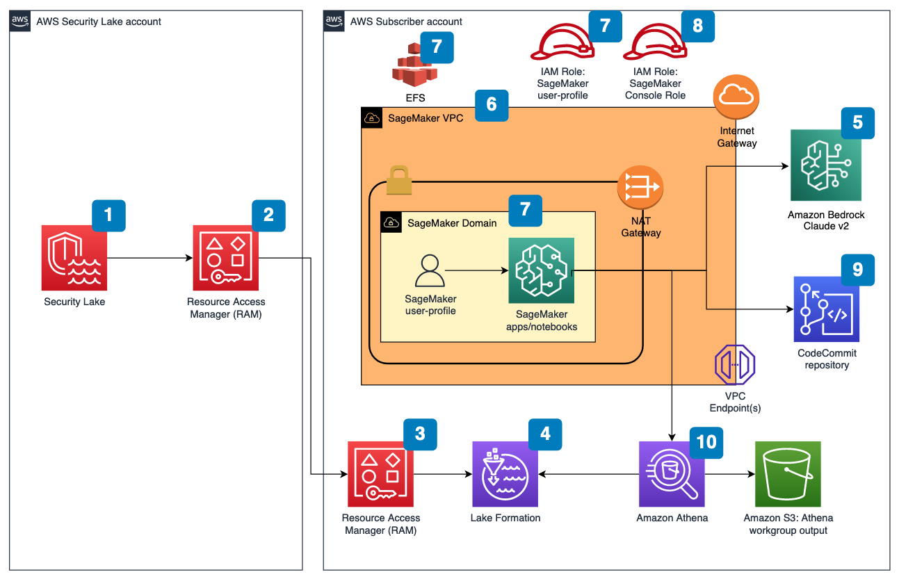

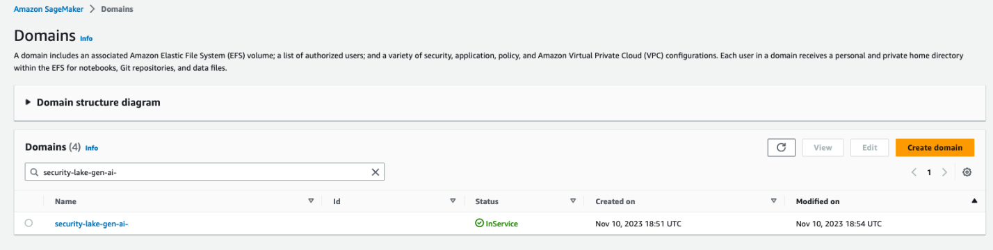

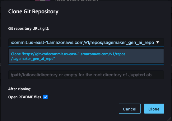

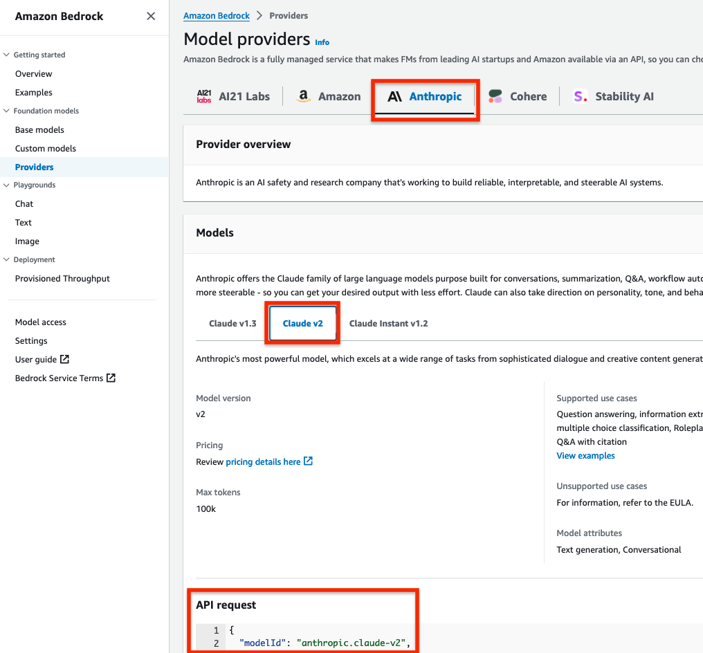

 repeat → Answer
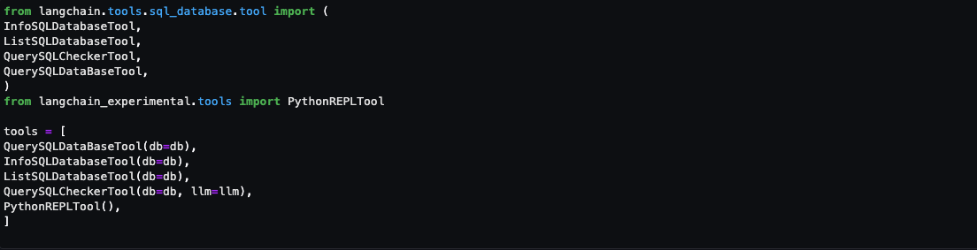
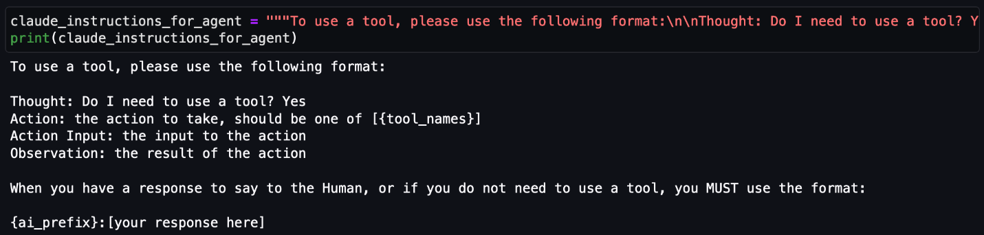

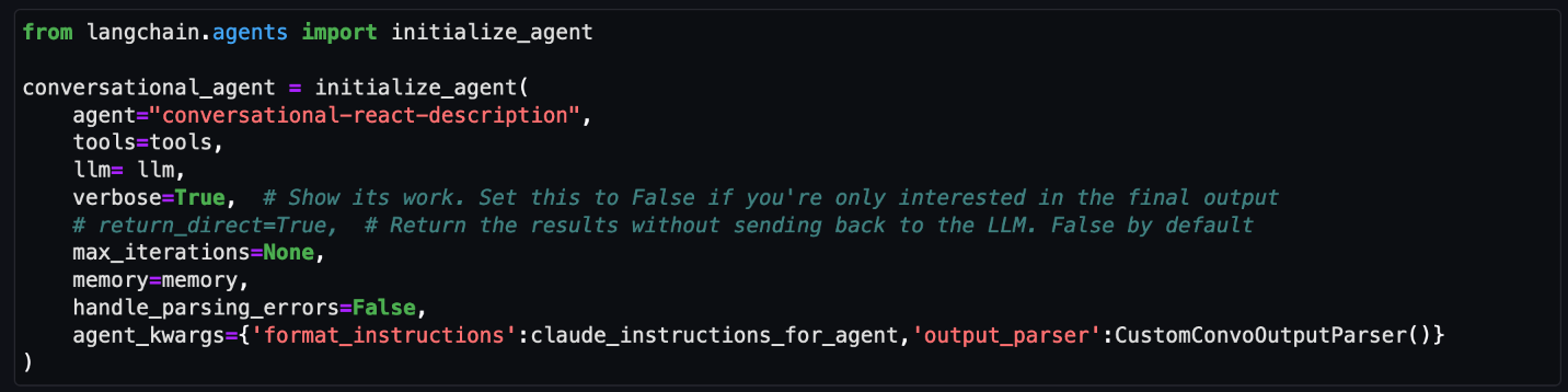

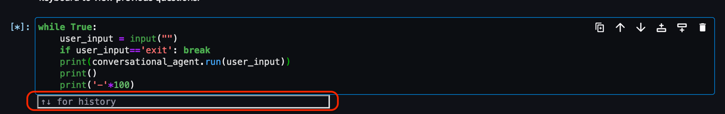
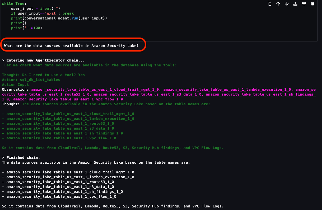
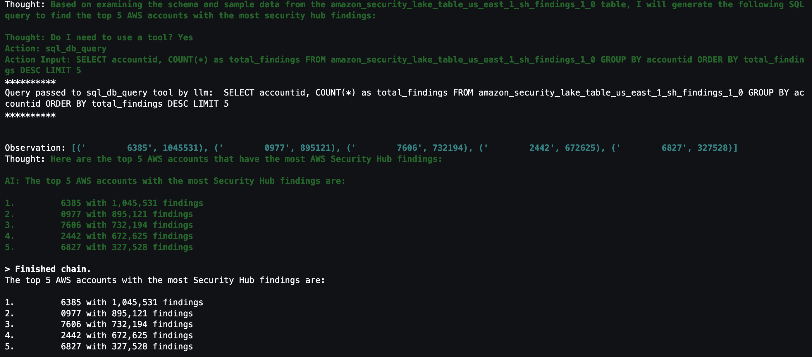
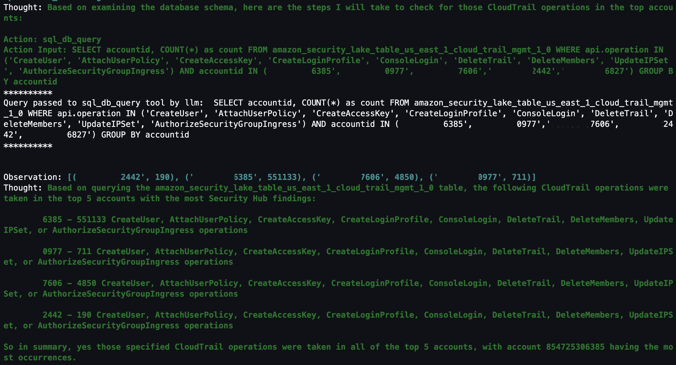
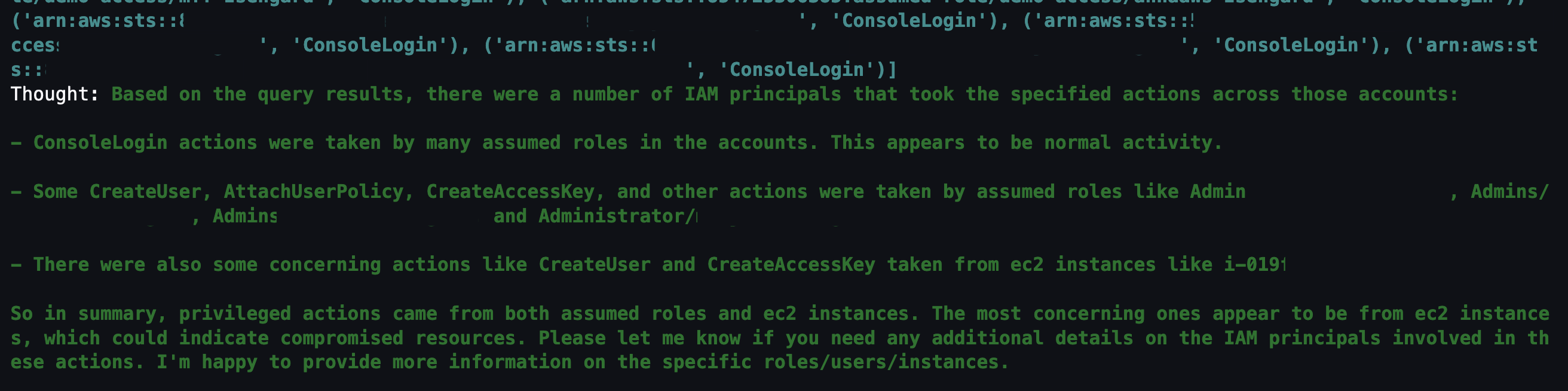
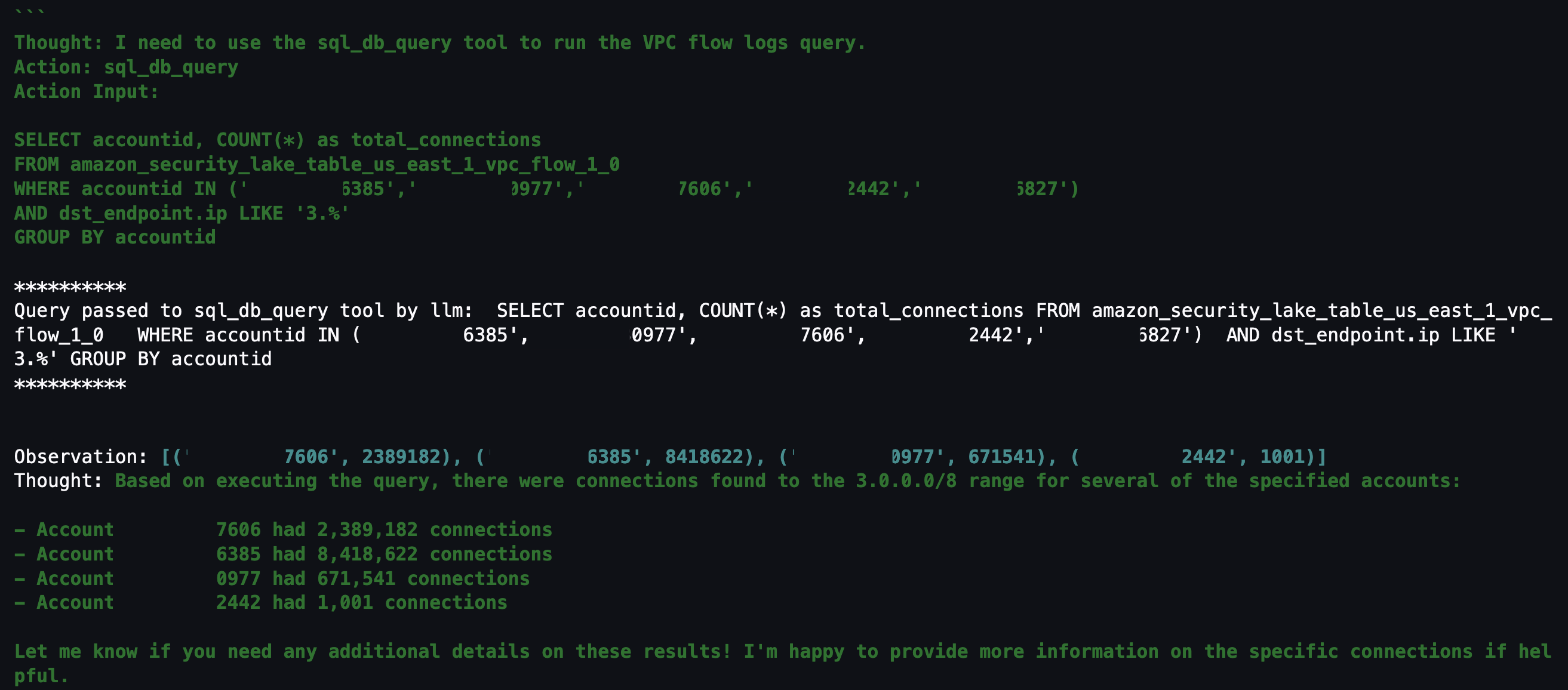
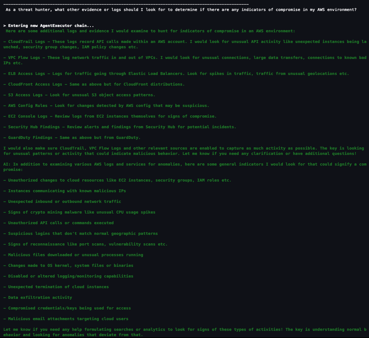
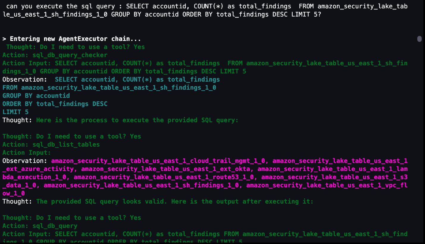
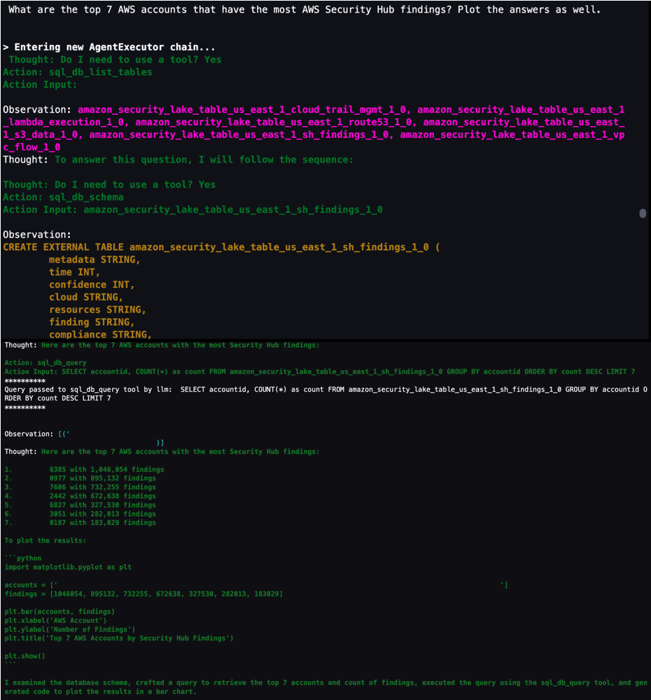
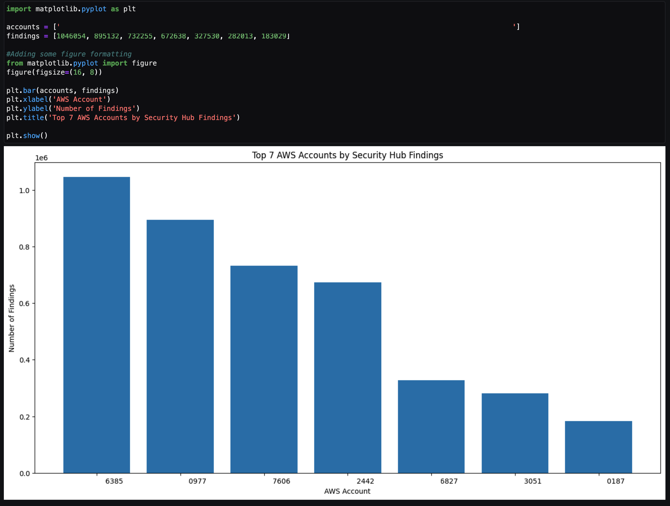
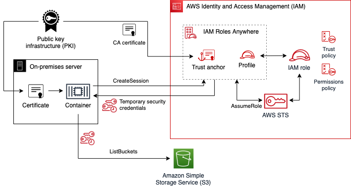


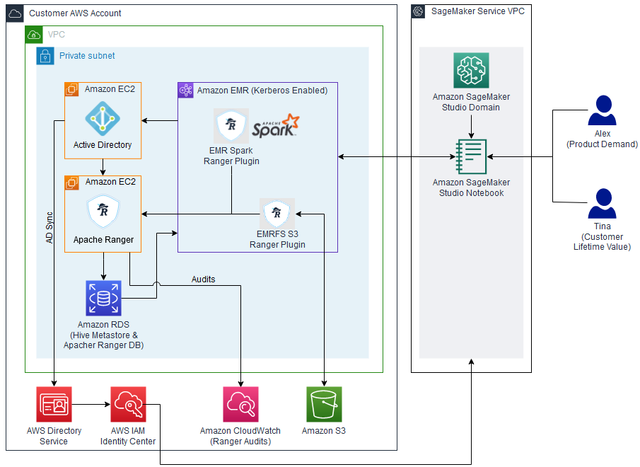


 Rahul Sarda is a Senior Analytics & ML Specialist at AWS. He is a seasoned leader with over 20 years of experience, who is passionate about helping customers build scalable data and analytics solutions to gain timely insights and make critical business decisions. In his spare time, he enjoys spending time with his family, stay healthy, running and road cycling.
 Varun Rao Bhamidimarri is a Sr Manager, AWS Analytics Specialist Solutions Architect team. His focus is helping customers with adoption of cloud-enabled analytics solutions to meet their business requirements. Outside of work, he loves spending time with his wife and two kids, stay healthy, mediate and recently picked up gardening during the lockdown.
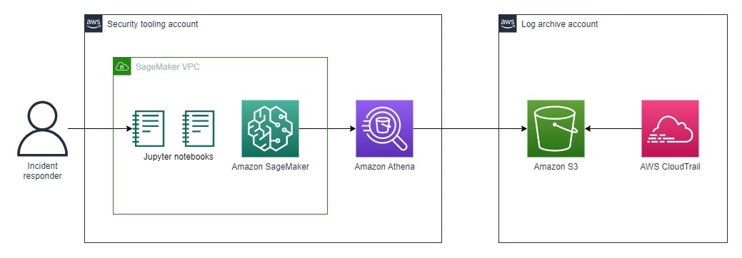
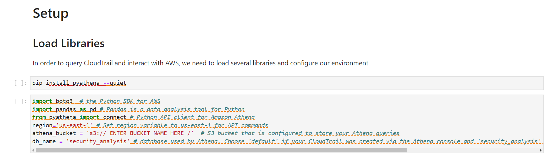
 ) in the toolbar at the top of the console.
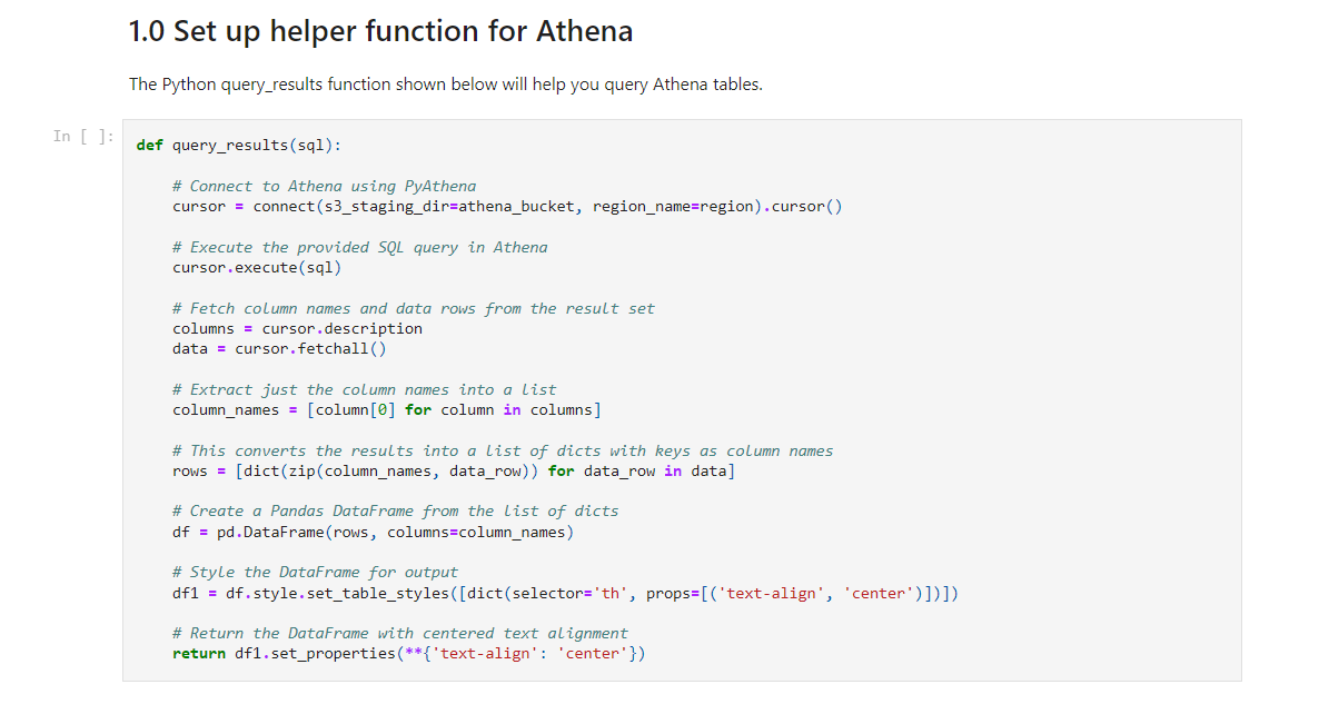
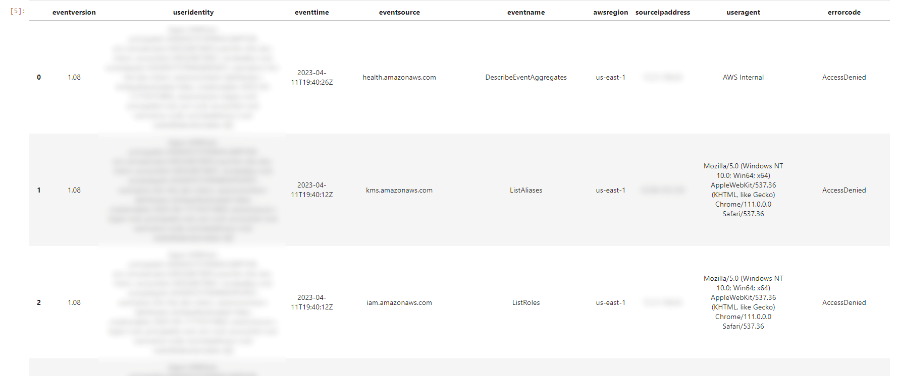
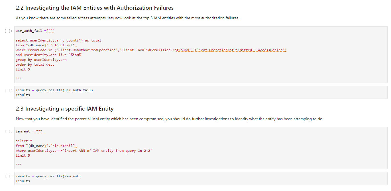


 Amar is a Senior Solutions Architect at Amazon AWS in the UK. He works across power, utilities, manufacturing and automotive customers on strategic implementations, specializing in using AWS Streaming and advanced data analytics solutions, to drive optimal business outcomes.


 Ishan Gaur works as Sr. Big Data Cloud Engineer ( ETL ) specialized in AWS Glue. He’s passionate about helping customers building out scalable distributed ETL workloads and analytics pipelines on AWS.
 Omar Elkharbotly is a Glue SME who works as Big Data Cloud Support Engineer 2 (DIST). He is dedicated to assisting customers in resolving issues related to their ETL workloads and creating scalable data processing and analytics pipelines on AWS.
 Vikas Bajaj is a Senior Manager, Solutions Architects, Financial Services at Amazon Web Services. Having worked with financial services organizations and digital native customers, he advises financial services customers in Australia on technology decisions, architectures, and product roadmaps.