Tag Archives: Field Notes

Field Notes: Accelerating Data Science with RStudio and Shiny Server on AWS Fargate

Post Syndicated from Chayan Panda original https://aws.amazon.com/blogs/architecture/field-notes-accelerating-data-science-with-rstudio-and-shiny-server-on-aws-fargate/

Data scientists continuously look for ways to accelerate time to value for analytics projects.  RStudio Server is a popular Integrated Development Environment (IDE) for R, which is used to render analytics visualizations for faster decision making. These visualizations are traditionally hosted on legacy unix servers along with Shiny Server to support analytics. In this previous blog, we provided a solution architecture to run Data Science use cases for medium to large enterprises across industry verticals.

In this post, we describe and deliver the infrastructure code to run a secure, scalable and highly available RStudio and Shiny Server installation on AWS. We use these services: AWS Fargate, Amazon Elastic Container Service (Amazon ECS), Amazon Elastic File System (Amazon EFS), AWS DataSync, and Amazon Simple Storage Service (Amazon S3). We will then demonstrate a Data Science use case in RStudio and create an application on Shiny. The use case discussed involves pre-processing a dataset, and training a machine learning model in RStudio. The goal is to build a shiny application to surface breast cancer prediction insights against a set of parameters to users.

Overview of solution

We show how to deploy a Open Source RStudio Server and a Shiny Server in a serverless architecture from an automated deployment pipeline built with AWS Developer Tools. This is illustrated in the diagram that follows. The deployment adheres to best practices for following an AWS Multi-Account strategy using AWS Organizations.

Figure 1. RStudio/Shiny Open Source Deployment Pipeline on AWS Serverless Infrastructure

Figure 1. RStudio/Shiny Open Source Deployment Pipeline on AWS Serverless Infrastructure

Multi-Account Setup

In the preceding architecture, a central development account hosts the development resources. From this account, the deployment pipeline creates AWS services for RStudio and Shiny along with the integrated services into another AWS account. There can be multiple RStudio/Shiny accounts and instances to suit your requirements. You can also host multiple non-production instances of RStudio/Shiny in a single account.

Public URL Domain and Data Feed

The RStudio/Shiny deployment accounts obtain the networking information for the publicly resolvable domain from a central networking account. The data feed for the containers comes from a central data repository account. Users upload data to the S3 buckets in the central data account or configure an automated service like AWS Transfer Family to programmatically upload files. AWS DataSync transfers the uploaded files from Amazon S3 and stores the files on Amazon EFS mount points on the containers. Amazon EFS provides shared, persistent, and elastic storage for the containers.

Security Footprint

We recommend that you configure AWS Shield or AWS Shield Advanced for the networking account and enable Amazon GuardDuty in all accounts. You can also use AWS Config and AWS CloudTrail for monitoring and alerting on security events before deploying the infrastructure code. You should use an outbound filter such as AWS Network Firewall for network traffic destined for the internet. AWS Web Application Firewall (AWS WAF) protects the Amazon Elastic Load Balancers (Amazon ELB). You can restrict access to RStudio and Shiny from only allowed IP ranges using the automated pipeline.

High Availability

You deploy all AWS services in this architecture in one particular AWS Region. The AWS services used are managed services and configured for high availability. Should a service become unavailable, it automatically launches in the same Availability Zone (AZ) or in a different AZ within the same AWS Region. This means if Amazon ECS restarts the container in another AZ, following a failover, the files and data for the container will not be lost as these are stored on Amazon EFS.

Deployment

The infrastructure code provided in this blog creates all resources described in the preceding architecture. The following numbered items refer to Figure 1.

1. We used AWS Cloud Development Kit (AWS CDK) for Python to develop the infrastructure code and stored the code in an AWS CodeCommit repository.
2. AWS CodePipeline integrates the AWS CDK stacks for automated builds. The stacks are divided into four different stages and are organized by AWS service.
3. AWS CodePipeline fetches the container images from public Docker Hub and stores the images into Amazon Elastic Container Registry (Amazon ECR) repositories for cross-account access. The deployment pipeline accesses these images to create the Amazon ECS container on AWS Fargate in the deployment accounts.
4. The build script uses a key from AWS Key Management Service (AWS KMS) to create secrets. These include a RStudio front-end password, public key for bastion containers, and central data account access keys in AWS Secrets Manager. The deployment pipeline uses these secrets to configure the cross-account containers.
5. The central networking account Amazon Route 53 has the pre-configured base public domain. This is done outside the automated pipeline and the base domain info is passed on as a parameter to the deployment pipeline.
6. The central networking account delegates the base public domain to the RStudio deployment accounts via AWS Systems Manager (SSM) Parameter Store.
7. An AWS Lambda function retrieves the delegated Route 53 zone for configuring the RStudio and Shiny sub-domains.
8. AWS Certificate Manager configures encryption in transit by applying HTTPS certificates on the RStudio and Shiny sub-domains.
9. The pipeline configures an Amazon ECS cluster to control the RStudio, Shiny and Bastion containers and to scale up and down the number of containers as needed.
10. The pipeline creates RStudio container for the instance in a private subnet. RStudio container is not horizontally scalable for the Open Source version of RStudio.
– If you create only one container, the container will be configured for multiple front-end users. You need to specify the user names as email ids in cdk.json.
– Users receive their passwords and Rstudio/Shiny URLs via emails using Amazon Simple Email Service (SES).
– You can also create one RStudio container for each Data Scientist depending on your compute requirements by setting the cdk.json parameter individual_containers to true. You can also control the container memory/vCPU using cdk.json.
– Further details are provided in the readme. If your compute requirements exceed Fargate container compute limits, consider using EC2 launch type of Amazon ECS which offers a range of Amazon EC2 servers to fit your compute requirement. You can specify your installation type in cdk.json and choose either Fargate or EC2 launcg type for your RStudio containers.
11. To help you SSH to RStudio and Shiny containers for administration tasks, the pipeline creates a Bastion container in the public subnet. A Security Group restricts access to the bastion container and you can only access it from the IP range you provide in the cdk.json.
12. Shiny containers are horizontally scalable and the pipeline creates the Shiny containers in the private subnet using Fargate launch type of Amazon ECS. You can specify the number of containers you need for Shiny Server in cdk.json.
13. Application Load Balancers route traffic to the containers and perform health checks. The pipeline registers the RStudio and Shiny load balancers with the respective Amazon ECS services.
14. AWS WAF rules are built to provide additional security to RStudio and Shiny endpoints. You can specify approved IPs to restrict access to RStudio and Shiny from only allowed IPs.
15. Users upload files to be analysed to a central data lake account either with manual S3 upload or programmatically using AWS Transfer for SFTP.
16. AWS DataSync transfers files from Amazon S3 to cross-account Amazon EFS on an hourly interval schedule.
17. An AWS Lambda initiates DataSync transfer on demand outside of the hourly schedule for files that require urgent analysis. It is expected that bulk of the data transfer will happen on the hourly schedule and on-demand trigger will only be used when necessary.
18. Amazon EFS file systems provide shared, persistent and elastic storage for the containers. This is to facilitate deployment of Shiny Apps from RStudio containers using shared file system. The EFS file systems will live through container recycles.
19. You can create Amazon Athena tables on the central data account S3 buckets for direct interaction using JDBC from the RStudio container. Access keys for cross account operation are stored in the RStudio container R environment.

Note: It is recommended that you implement short term credential vending for this operation.

The source code for this deployment can be found in the aws-samples GitHub repository.

Prerequisites

To deploy the cdk stacks from the source code, you should have the following prerequisites:

1. Access to four AWS accounts (minimum three) for a basic multi-account deployment.
2. Permission to deploy all AWS services mentioned in the solution overview.
3. Review RStudio and Shiny Open Source Licensing: AGPL v3 (https://www.gnu.org/licenses/agpl-3.0-standalone.html)
4. Basic knowledge of R, RStudio Server, Shiny Server, Linux, AWS Developer Tools (AWS CDK in Python, AWS CodePipeline, AWS CodeCommit), AWS CLI and, the AWS services mentioned in the solution overview
5. Ensure you have a Docker hub login account, otherwise you might get an error while pulling the container images from Docker Hub with the pipeline – You have reached your pull rate limit. You may increase the limit by authenticating and upgrading: https://www.docker.com/increase-rate-limits.
6. Review the readmes delivered with the code and ensure you understand how the parameters in cdk.json control the deployment and how to prepare your environment to deploy the cdk stacks via the pipeline detailed below.

Installation

Create the AWS accounts to be used for deployment and ensure you have admin permissions access to each account. Typically, the following accounts are required:

Central Development account – this is the account where the AWS Secret Manager parameters, AWS CodeCommit repository, Amazon ECR repositories, and AWS CodePipeline will be created.
Central Network account – the Route53 base public domain will be hosted in this account
Rstudio instance account – You can use as many of these accounts as required, this account will deploy RStudio and Shiny containers for an instance (dev, test, uat, prod) along with a bastion container and associated  services as described in the solution architecture.
Central Data account – this is the account to be used for deploying the data lake resources – such as S3 bucket for selecting up ingested source files.

1. Install AWS CLI and create an AWS CLI profile for each account (pipeline, rstudio, network, datalake ) so that AWS CDK can be used.
2. Install AWS CDK in Python and bootstrap each account and allow the Central Development account to perform cross-account deployment to all the other accounts.

export CDK_NEW_BOOTSTRAP=1
npx cdk bootstrap --profile <AWS CLI profile of central development account> --cloudformation-execution-policies arn:aws:iam::aws:policy/AdministratorAccess aws://<Central Development Account>/<Region>

cdk bootstrap \
--profile <AWS CLI profile of rstudio deployment account> \
--trust <Central Development Account> \
--cloudformation-execution-policies arn:aws:iam::aws:policy/AdministratorAccess \
aws://<RStudio Deployment Account>/<Region>

cdk bootstrap \
--profile <AWS CLI profile of central network account> \
--trust <Central Development Account> \
--cloudformation-execution-policies arn:aws:iam::aws:policy/AdministratorAccess \
aws://<Central Network Account>/<Region>

cdk bootstrap \
--profile <AWS CLI profile of central data account> \
--trust <Central Development Account> \
--cloudformation-execution-policies arn:aws:iam::aws:policy/AdministratorAccess \
aws://<Central Data Account>/<Region>

3. Build the Docker container images in Amazon ECR in the central development account by running the image build pipeline as instructed in the readme.
a. Using the AWS console, create an AWS CodeCommit repository to hold the source code for building the images – for example, rstudio_docker_images.
b. Clone the GitHub repository and move into the image-build folder.
c. Using the CLI – Create a secret to store your DockerHub login details as follows:

aws secretsmanager create-secret --profile <AWS CLI profile of central development account> --name ImportedDockerId --secret-string '{"username":"<dockerhub username>", "password":"<dockerhub password>"}'

d. Create an AWS CodeCommit repository to hold the source code for building the images – e.g. rstudio_docker_images and pass the repository name to the name parameter in cdk.json for the image build pipeline
e. Pass the account numbers (comma separated) where rstudio instances will be deployed in the cdk.json paramter rstudio_account_ids
f. Synthesize the image build stack

cdk synth --profile <AWS CLi profile of central development account>

g. Commit the changes into the AWS CodeCommit repo you created using GitHub.
h. Deploy the pipeline stack for container image build.

cdk deploy --profile <AWS CLI profile of central development account>

i. Log into AWS console in the central development account and navigate to CodePipeline service. Monitor the pipeline (pipeline name is the name you provided in the name parameter in cdk.json) and confirm the docker images build successfully.

4. Move into the rstudio-fargate folder. Provide the comma separated accounts where rstudio/shiny will be deployed in the cdk.json against the parameter rstudio_account_ids.

5. Synthesize the stack Rstudio-Configuration-Stack in the Central Development account.

cdk synth Rstudio-Configuration-Stack --profile <AWS CLI profile of central development account> 

6. Deploy the Rstudio-Configuration-Stack. This stack should create a new CMK KMS Key to use for creating the secrets with AWS Secrets Maanger. The stack will output the AWS ARN for the KMS key. Note down the ARN. Set the parameter “encryption_key_arn” inside cdk.json to the above ARN.

cdk deploy Rstudio-Configuration-Stack --profile <AWS CLI profile of rstudio deployment account>

7. Run the script rstudio_config.sh after setting the required cdk.json parameters. Refer readme.

sh ./rstudio_config.sh <AWS CLI profile of the central development account> "arn:aws:kms:<region>:<AWS CLI profile of central development account>:key/<key hash>" <AWS CLI profile of central data account> <comma separated AWS CLI profiles of the rstudio deployment accounts>

8. Run the script check_ses_email.sh with comma separated profiles for rstudio deployment accounts. This will check whether all user emails have been registed with Amazon SES for all the rstudio deployment accounts in the region, before you can deploy rstudio/shiny.

sh ./check_ses_email.sh <comma separated AWS CLI profiles of the rstudio deployment accounts>

9. Before committing the code into the AWS CodeCommit repository, synthesize the pipeline stack against all the accounts involved in this deployment. This ensures all the necessary context values are populated into cdk.context.json file and to avoid the DUMMY values being mapped.

cdk synth --profile <AWS CLI profile of the central development account>
cdk synth --profile <AWS CLI profile of the central network account>
cdk synth --profile <AWS CLIrepeat for each profile of the RStudio deplyment account>

10. Deploy the Rstudio Fargate pipeline stack.

cdk deploy --profile <AWS CLI profile of the central development account> Rstudio-Piplenine-Stack

Data Science use case

Now the installation is completed. We can demonstrate a typical data science use case:

  1. Explore, and pre-process a dataset, and train a machine learning model in RStudio,
  2. Build a Shiny application that makes prediction against the trained model to surface insight to dashboard users.

This showcases how to publish a Shiny application from RStudio containers to Shiny containers via a common EFS filesystem.

First, we log on to the RStudio container with the URL from the deployment and clone the accompanying repository using the command line terminal. The ML example is in ml_example directory. We use the UCI Breast Cancer Wisconsin (Diagnostic) dataset from mlbench library. Refer to the ml_example/breast_cancer_modeling.r.

$ git clone https://github.com/aws-samples/aws-fargate-with-rstudio-open-source.git
Figure 2. Use the terminal to clone the repository in RStudio IDE.

Figure 2 – Use the terminal to clone the repository in RStudio IDE.

Let’s open the ml_example/breast_cancer_modeling.r script in the RStudio IDE. The script does the following:

  1. Install and import the required libraries, mainly caret, a popular machine learning library, and mlbench, a collection of ML datasets;
  2. Import the UCI breast cancer dataset, create an 80/20 split for training and testing (in shiny app) purposes;
  3. Perform preprocessing to impute the missing values (shown as NA) in the dataframe and standardize the numeric columns;
  4. Train a stochastic gradient boosting model with cross-validation with the area under the ROC curve (AUC) as the tuning metric;
  5. Save the testing split, preprocessing object and the trained model into the directory where shiny app script is located/breast-cancer-prediction.

You can execute the whole script with this command in the console.

> source('~/aws-fargate-with-rstudio-open-source/ml_example/breast_cancer_modeling.r')

We can then inspect the model evaluation in the model object gbmFit.

> gbmFit
Stochastic Gradient Boosting 

560 samples
  9 predictor
  2 classes: 'benign', 'malignant' 

No pre-processing
Resampling: Cross-Validated (10 fold, repeated 10 times) 
Summary of sample sizes: 504, 505, 503, 504, 504, 504, ... 
Resampling results across tuning parameters:

  interaction.depth  n.trees  ROC        Sens       Spec     
  1                   50      0.9916391  0.9716967  0.9304474
  1                  100      0.9917702  0.9700676  0.9330789
  1                  150      0.9911656  0.9689790  0.9305000
  2                   50      0.9922102  0.9708859  0.9351316
  2                  100      0.9917640  0.9681682  0.9346053
  2                  150      0.9910501  0.9662613  0.9361842
  3                   50      0.9922109  0.9689865  0.9381316
  3                  100      0.9919198  0.9684384  0.9360789
  3                  150      0.9912103  0.9673348  0.9345263

If the results are as expected, move on to developing a dashboard and publishing the model for business users to consume the machine learning insights.

In the repository, ml_example/breast-cancer-prediction/app.R has a Shiny application that displays a summary statistics and distribution of the testing data, and an interactive dashboard. This allows users to select data points on the chart and understand get the machine learning model inference as needed. Users can also modify the threshold to alter the specificity and sensitivity of the prediction. Thanks to the shared EFS filesystem across the RStudio and Shiny containers, we can publish the Shiny application with the following shell command to /srv/shiny-server.

$ cp ~/aws-fargate-with-rstudio-open-source/ml_example/breast-cancer-prediction/ \ /srv/shiny-server/ -rfv

That’s it. The Shiny application is now on the Shiny containers accessible from the Shiny URL, load balanced by Application Load Balancer. You can slide over the Probability Threshold to test how it changes the total count in the prediction, change the variables for the scatter plot and select data points to test the individual predictions.

shiny-dashboard-breast-cancer

Figure 3 – The Shiny Application

Cleaning up

Please follow the readme in the repository to delete the stacks created.

Conclusion

In this blog, we demonstrated how a serverless architecture can be deployed, walked through a data science use case in RStudio server and deployed an interactive dashboard in Shiny server. The solution creates a scalable, secure, and serverless data science environment for the R community that accelerates the data science process. The infrastructure and data science code is available in the github repository.

Field Notes provides hands-on technical guidance from AWS Solutions Architects, consultants, and technical account managers, based on their experiences in the field solving real-world business problems for customers.


Field Notes: SQL Server Deployment Options on AWS Using Amazon EC2

Post Syndicated from Saqlain Tahir original https://aws.amazon.com/blogs/architecture/field-notes-sql-server-deployment-options-on-aws-using-amazon-ec2/

Many enterprise applications run Microsoft SQL Server as their backend relational database.  There are various options for customers to benefit from deploying their SQL Server on AWS. This blog will help you choose the right architecture for your SQL Server Deployment with high availability options, using Amazon EC2 for mission-critical applications.

SQL Server on Amazon EC2 offers more efficient control of deployment options and enables customers to fine-tune their Microsoft workload performance with full control. Most importantly you can bring your own licenses (BYOL) on AWS. You can re-host, aka “lift and shift”, your SQL Server to Amazon Elastic Compute Cloud (Amazon EC2) for large scale Enterprise applications. If you are re-hosting, you can still use your existing SQL Server license on AWS. Lifting and shifting your on-premises MS SQL Server environment to AWS using Amazon EC2 is recommended to migrate your SQL Server workloads to the cloud.

First, it is important to understand the considerations for deploying a SQL Server using Amazon EC2. For example, when would you want to use Failover Cluster over Availability Groups?

The following table will help you to choose the right architecture for SQL Server architecture based on the type of workload and availability requirements:

Following table will help you to choose the right architecture for SQL Server architecture based on the type of workload and high availability requirements:

Self-managed MS SQL Server on EC2 usually means hosting MS SQL on EC2 backed by Amazon Elastic Block Store (EBS) or Amazon FSx for Windows File Server. Persistent storage from Amazon EBS and Amazon FSx delivers speed, security, and durability for your business-critical relational databases such as Microsoft SQL Server.

  • Amazon EBS delivers highly available and performant block storage for your most demanding SQL Server deployments to achieve maximum performance.
  • Amazon FSx delivers fully managed Windows native shared file storage (SMB) with a multi-Availability Zone (AZ) design for highly available (HA) SQL environments.

Previously, if you wanted to migrate your Failover Cluster SQL databases to AWS, there was no native shared storage option. You would need to implement third party solutions that added a cost and complexity to install, set up, and maintain the storage configuration.

Amazon FSx for Windows File Server provides shared storage that multiple SQL databases can connect to across multiple AZs for a DR and HA solution. It is also helpful to achieve throughput and certain IOPS without scaling up the instance types to get the same IOPS from EBS volumes.

Overview of solution

Most customers need High Availability (HA) for their SQL Server production environment to ensure uptime and availability. This is important to minimize changes to the SQL Server applications while migrating. Customers may want to protect their investment in Microsoft SQL Server licenses by taking a Bring your own license (BYOL) approach to cloud migration.

There are some scenarios where applications running on Microsoft SQL Server need full control of the infrastructure and software. If customers require it, they can deploy their SQL Server to AWS on Amazon EC2. Currently, there are three ways to deploy SQL Server workloads on AWS as shown in the following diagram:

There are some scenarios where applications running on Microsoft SQL Server need full control of the infrastructure and software. If customers require it, they can deploy their SQL Server to AWS on Amazon EC2. Currently, there are various ways to deploy SQL Server workloads on AWS as shown in the following diagram:

Walkthrough

Now the question comes, how do you deploy the preceding SQL Server architectures?

First, let’s discuss the high-level breakdown of deployment options including the two types of SQL HA modes:

  • Standalone
    • Single SQL Server Node without HA
    • Provision Amazon EC2 instance with EBS volume
    • Single Availability Zone deployment
  • Always On Failover Cluster Instance (FCI): EC2 and FSx for Windows File Server
    • Protects the whole instance, including system databases
    • Failovers over at the instance level
    • Requires Shared Storage, Amazon FSx for Windows File Server is a great option
    • Can be used in conjunction with Availability Groups to provide read-replicas and DR copies (dependent upon SQL Server Edition)
    • Can be implemented at the Enterprise or Standard Edition level (with limitations)
    • Multi Availability Zone Deployment
  • Always On Availability Groups (AG): EC2 and EBS
    • Protects one or more user databases (Standard Edition is limited to a single user database per AG)
    • Failover is at the Availability Group level, meaning potentially only a subset of user databases can failover versus the whole instance
    • System databases are not replicated, meaning users, jobs etc. will not automatically appear on passive nodes, manual creation is needed on all nodes
    • Natively provides access to read-replicas and DR copies (dependent upon Edition)
    • Can be implemented at the Enterprise or Standard
    • Multi Availability Zone Deployment

Prerequisites

For this walkthrough, you should have the following prerequisites:

  • An AWS account
  • SQL Server Licenses in case of BYOL Deployment
  • Identify Software and Hardware requirements for SQL Server Environment
  • Identify SQL Server application requirements based on best practices in this deployment guide

Deployment options on AWS

Here are some tools and services provided by AWS to deploy the SQL Server production ready environment by following best practices.

SQL Server on the AWS Cloud: Quick Start Reference Deployment

Use Case:

You want to deploy SQL Server on AWS for a Proof of Concept (PoC) or Pilot deployment using CloudFormation templates within hours by following these best practices.

Overview:

The Quick Start deployment guide provides step-by-step instructions for deploying SQL Server on the Amazon Web Services (AWS) Cloud, using AWS CloudFormation templates and AWS Systems Manager Automation documents that automate the deployment.

SQL Server on the AWS Cloud: Quick Start Reference Deployment

Implementation:

Quick Start Link: SQL Server with WSFC Quick Start

Source Code: GitHub

SQL Server Always On Deployments with AWS Launch Wizard

Use Case:

You intend to deploy SQL Server on AWS for your production workloads to benefit from automation, time and cost savings, and most importantly by leveraging proven deployment best practices from AWS.

Overview:

AWS Launch Wizard is a service that guides you through the sizing, configuration, and deployment of Microsoft SQL Server applications on AWS, following the AWS Well-Architected Framework. AWS Launch Wizard supports both single instance and high availability (HA) application deployments.

AWS Launch Wizard reduces the time it takes to deploy SQL Server solutions to the cloud. You input your application requirements, including performance, number of nodes, and connectivity, on the service console. AWS Launch Wizard identifies the right AWS resources to deploy and run your SQL Server application. You can also receive an estimated cost of deployment, modify your resources and instantly view the updated cost assessment.

When you approve, AWS Launch Wizard provisions and configures the selected resources in a few hours to create a fully-functioning production-ready SQL Server application. It also creates custom AWS CloudFormation templates, which can be reused and customized for subsequent deployments.

Once deployed, your SQL Server application is ready to use and can be accessed from the EC2 console. You can manage your SQL Server application with AWS Systems Manager.

SQL Server Always On Deployments with AWS Launch Wizard

Implementation:

AWS Launch Wizard Link: AWS Launch Wizard for SQL Server

Simplify your Microsoft SQL Server high availability deployments using Amazon FSx for Windows File Server

Use Case:

You need SQL enterprise edition to run an Always on Availability Group (AG), whereas you only need the standard edition to run Failover Cluster Instance (FCI). You want to use standard licensing to save costs but want to achieve HA. SQL Server Standard is typically 40–50% less expensive than the Enterprise Edition.

Overview:

Always On Failover Cluster (FCI) uses block level replication rather than database-level transactional replication. You can migrate to AWS without re-architecting. As the shared storage handles replication you don’t need to use SQL nodes for it, and frees up CPU/Memory for primary compute jobs. With FCI, the entire instance is protected – if the primary node becomes unavailable, the entire instance is moved to the standby node. This takes care of the SQL Server logins, SQL Server Agent jobs, and certificates that are stored in the system databases. These are physically stored in shared storage.

Simplify your Microsoft SQL Server high availability deployments using Amazon FSx for Windows File Server

Implementation:

FCI implementation: SQL Server Deployment using FCI, FSx QuickStart.

Clustering for SQL Server High Availability using SIOS Data Keeper

Use Case:

Windows Server Failover Clustering is a requirement if you are using SQL Server Enterprise or the SQL Server Standard edition and it might appear to be the perfect HA solution for applications running on Windows Server. But like FCIs, it requires the use of shared storage. If you want to use software SAN across multiple instances, then SIOS Data Keeper can be an option.

Overview:

WSFC has a potential role to play in many HA configurations, including for SQL Server FCIs, but its use requires separate data replication provisions in a SANless environment, whether in an enterprise datacenter or in the cloud.  SIOS data keeper is a partner solution software SAN across multiple instances. Instead of FSx, you deploy another cluster for SIOS data keeper to host the shared volumes or use a hyper-converged model to deploy SQL Server on the same server as the SIOS data keeper. You can also use SIOS DataKeeper Cluster Edition, a highly optimized, host-based replication solution.

Clustering for SQL Server High Availability using SIOS Data Keeper

Implementation:

QuickStart: SIOS DataKeeper Cluster Edition on the AWS Cloud

Conclusion

In this blog post, we covered the different options of SQL Server Deployment on AWS using EC2. The options presented showed how you can have the exact same experience from an administration point of view, as well as full control over your EC2 environment, including sysadmin and root-level access.

We also showed various ways to achieve High Availability, by deploying SQL Server on AWS as a new environment using AWS QuickStart and AWS Launch Wizard. We  also showed how you can deploy SQL Server using AWS managed windows storage Amazon FSx to handle shared storage constraint, cost and IOPS requirement scenarios. If you need shared storage in the cloud outside the Windows FSx option, AWS supports a partner solution using SIOS DataKeeper Cluster Edition.

We hope you found this blog post useful and welcome your feedback in the comments!

Field Notes provides hands-on technical guidance from AWS Solutions Architects, consultants, and technical account managers, based on their experiences in the field solving real-world business problems for customers.

Field Notes: Develop Data Pre-processing Scripts Using Amazon SageMaker Studio and an AWS Glue Development Endpoint

Post Syndicated from Sam Mokhtari original https://aws.amazon.com/blogs/architecture/field-notes-develop-data-pre-processing-scripts-using-amazon-sagemaker-studio-and-an-aws-glue-development-endpoint/

This post was co-written with Marcus Rosen, a Principal  – Machine Learning Operations with Rio Tinto, a global mining company. 

Data pre-processing is an important step in setting up Machine Learning (ML) projects for success. Many AWS customers use Apache Spark on AWS Glue or Amazon EMR to run data pre-processing scripts while using Amazon SageMaker to build ML models.  To develop spark scripts in AWS Glue, you can create an environment called a Glue Development (Dev) Endpoint that lets you author and test your data pre-processing scripts iteratively. When you’re satisfied with the results of your development, you can create a Glue ETL job that runs the final script as part of your automation framework.

With the introduction of Amazon SageMaker Studio in AWS re:Invent 2020, you can now use a single web-based IDE to spin up a notebook and perform all ML development steps. These include data pre-processing, ML model training, ML model deployment and monitoring.

This post walks you through how to connect a SageMaker Studio notebook to an AWS Glue Dev Endpoint, so you can use a single tool to iteratively develop both data pre-processing scripts and ML models.

Solution Overview

The following diagram shows the components that are used in this solution.

  • First, we use an AWS CloudFormation template to set up the required networking components (for example, VPC, subnets).
  • Then, we create an AWS Glue Dev Endpoint and use a security group to allow SageMaker Studio to securely access the endpoint.
  • Finally, we create a studio domain and use a SparkMagic kernel to connect to the AWS Glue Dev Endpoint and run spark scripts.

In the Amazon SageMaker Studio notebook, SparkMagic will call a REST API against a Livy server running on the AWS Glue Dev Endpoint. Apache Livy is a service that enables interaction with a remote Spark cluster over a REST API.


The following diagram shows the components that are used in this solution. We use an AWS CloudFormation template to set up the required ntworking components (for example, VPC, subnets).

Set up the VPC

You can use the following CloudFormation template to set up the environment needed for this solution.

launch stack button

This template deploys the following resources in your account:

  • A new VPC, with both public and private subnet.
  • VPC endpoints for the following resources:
  • Security groups for SageMaker Studio, Glue endpoint and VPC endpoints
  • SageMaker Service IAM role
  • AWS Glue Dev Endpoint IAM role
  • Set up the AWS Glue Dev Endpoint

Set up AWS Glue Dev Endpoint

Review this Developer Guide: Adding a Development Endpoint for instructions to create an AWS Glue Dev Endpoint.

Note: you must use the AWS Glue Dev Endpoint IAM role provisioned by the CloudFormation template.

  • In the Networking section, select Choose a VPC, subnet, and security groups.

Then choose the VPC glue security group, which you provisioned through the CloudFormation template.

The AWS Glue Dev Endpoint needs to be secured with an SSH public key, which should be generated within your local environment. An SSH key pair (public/private) can be generated using the ssh-keygen on Linux or using PuTTYgen on Windows.

Glue Dev Endpoint screenshot

The final review page looks similar to the following screenshot.

Final review page

Once the AWS Glue Dev Endpoint is in Ready status, keep note of its private IP address (Glue -> ETL -> Dev Endpoints). You will use this IP for the Livy port forwarding.

Set up SageMaker Studio

We recommend launching the SageMaker Studio resource by following the instructions in Securing Amazon SageMaker Studio connectivity using a private VPC .

Follow these steps when you provision the SageMaker Studio resources:

  • Select Standard setup with the AWS Identity and Access Management (IAM) authentication method.
  • Attach a SageMaker Service IAM role, created by the CloudFormation template, to SageMaker Studio.
  • Under Network and storage, select the same VPC and private subnet as the AWS Glue endpoint.
  • For the Network Access for Studio option, select VPC Only — SageMaker Studio will use your VPC. Direct internet access is disabled.

Then ensure that the security group with the self-referencing rule is attached. Also, check your other required security groups are attached for SageMaker Studio from the CloudFormation template output.

Connect the SageMaker Studio notebook to the AWS Glue Dev Endpoint

Once you launch the SageMaker Studio and you add the users. Follow these steps to connect the SageMaker Studio notebook to the AWS Glue Dev Endpoint:

  1. Open the Studio and go to the launcher page (by pressing the “+” icon on the top-left of the page.
  2. Under Notebooks and compute resources, select SparkMagic in the dropdown menu and select Notebook.
  3. Then open another launcher page, select SparkMagic in the same dropdown menu and select Image terminal. One thing to note is that the SparkMagic app will take some time to initialize. Proceed once the apps are in Ready status (2-3 minutes).

Notebooks and compute resources screenshot

4. Upload the private key into SparkMagic Image terminal. In other words, copy the private key to “.ssh” directory and update its permissions using “chmod 400”.

Note: the private key is corresponding to the public key used when you create the AWS Glue Dev Endpoint.

5. Now, you need to achieve port forwarding of the Livy service in order for SparkMagic kernel to be able to connect to the AWS Glue Dev Endpoint.  You run the following command in the image terminal:

/usr/bin/ssh -4 -N -o ServerAliveInterval=60 -o ServerAliveCountMax=3 -o StrictHostKeyChecking=no -i /root/.ssh/{PRIVATE_KEY} -L 8998:169.254.76.1:8998 glue@{GLUE_ENDPOINT_PRIVATE_IP_ADDRESS}

The command consists of:

  • {PRIVATE_KEY} is the private key file name that you copied into .ssh directory.
  • {GLUE_ENDPOINT_PRIVATE_IP_ADDRESS} is the private IP address of the AWS Glue Dev Endpoint.
  • “8998” is the Livy port we are using for port forwarding.
  • “169.254.76.1” is the remote IP address defined by AWS Glue, this IP address does not change.

Note: Keep this terminal open and the SSH command running in order to keep the Livy session active.

6. Go to the SparkMagic notebook and restart the kernel, by going to the top menu and selecting Kernel > Restart Kernel.

7. Once the notebook kernel is restarted, the connection between the Studio Notebook and the AWS Glue Dev Endpoint is ready. To test the integration, you can run the following example command to list the tables in the AWS Glue Data Catalog.

spark.sql("show tables").show()

To test the integration, you can run the following command to list the tables in the Glue Data Catalog

Cleaning up

To avoid incurring future charges, delete the resources you created:

Conclusion

Our customers needed a single web-based IDE to spin up a notebook and perform all ML development steps including data pre-processing, ML model training, ML model deployment and monitoring. This blog post demonstrated how you can configure a SageMaker Studio notebook and connect to AWS Glue Dev Endpoint. This provides a framework for you to use  when developing both data preprocessing scripts and ML models.

To learn more about how to develop data pre-processing scripts and ML models in Amazon SageMaker, you can check out the examples in this repository.

Field Notes provides hands-on technical guidance from AWS Solutions Architects, consultants, and technical account managers, based on their experiences in the field solving real-world business problems for customers.


Field Notes: Benchmarking Performance of the New M5zn, D3, and R5b Instance Types with Datadog

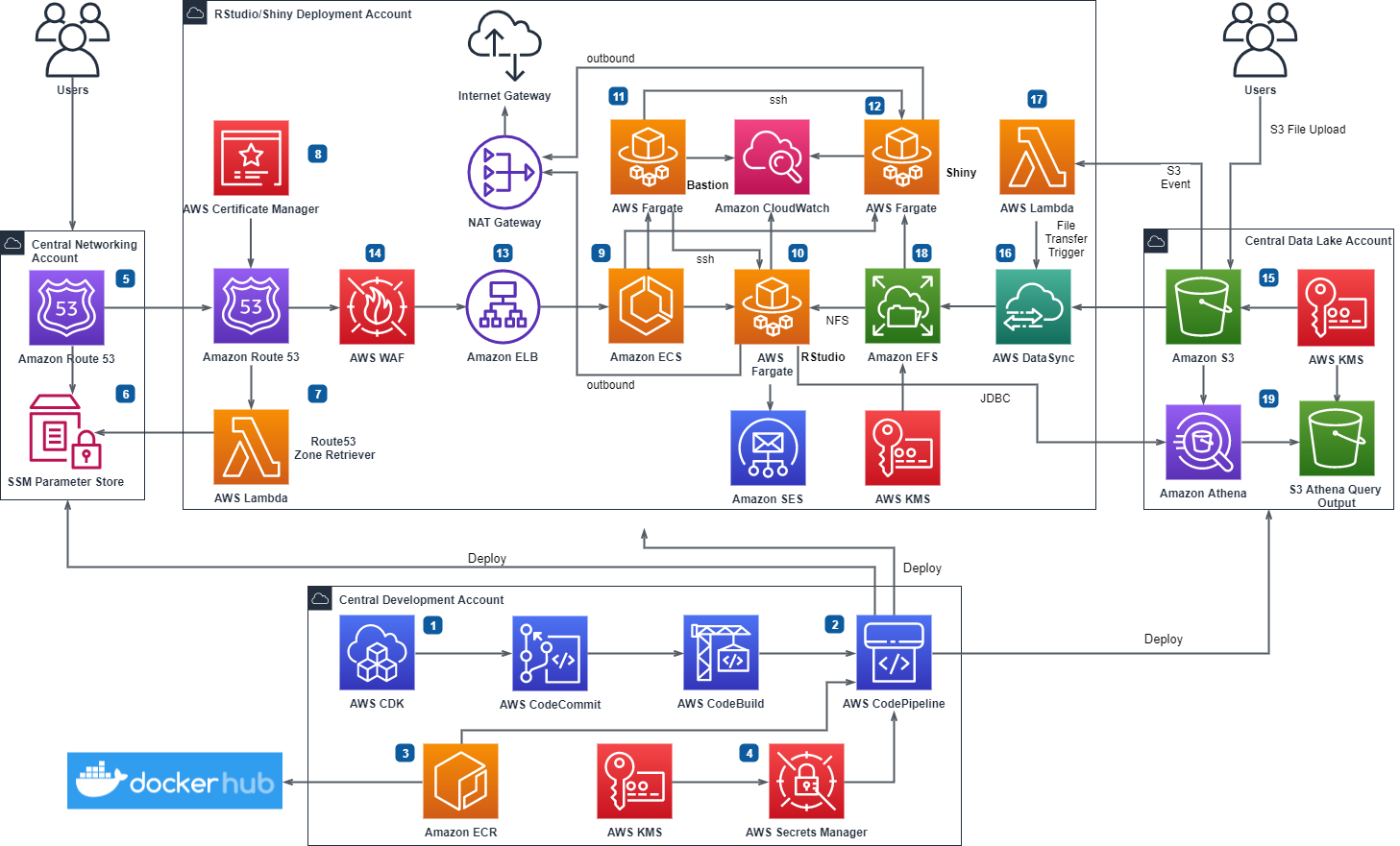
Post Syndicated from Ray Zaman original https://aws.amazon.com/blogs/architecture/field-notes-benchmarking-performance-of-the-new-m5zn-d3-and-r5b-instance-types-with-datadog/

This post was co-written with Danton Rodriguez, Product Manager at Datadog. 

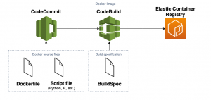
At re:Invent 2020, AWS announced the new Amazon Elastic Compute Cloud (Amazon EC2) M5zn, D3, and R5b instance types. These instances are built on top of the AWS Nitro System, a collection of AWS-designed hardware and software innovations that enable the delivery of private networking, and efficient, flexible, and secure cloud services with isolated multi-tenancy.

If you’re thinking about deploying your workloads to any of these new instances, Datadog helps you monitor your deployment and gain insight into your entire AWS infrastructure. The Datadog Agent—open-source software available on GitHub—collects metrics, distributed traces, logs, profiles, and more from Amazon EC2 instances and the rest of your infrastructure.

How to deploy Datadog to analyze performance data

The Datadog Agent is compatible with the new instance types. You can use a configuration management tool such as AWS CloudFormation to deploy it automatically across all your instances. You can also deploy it with a single command directly to any Amazon EC2 instance. For example, you can use the following command to deploy the Agent to an instance running Amazon Linux 2:

DD_AGENT_MAJOR_VERSION=7 DD_API_KEY=[Your API Key] bash -c "$(curl -L https://raw.githubusercontent.com/DataDog/datadog-agent/master/cmd/agent/install_script.sh)"

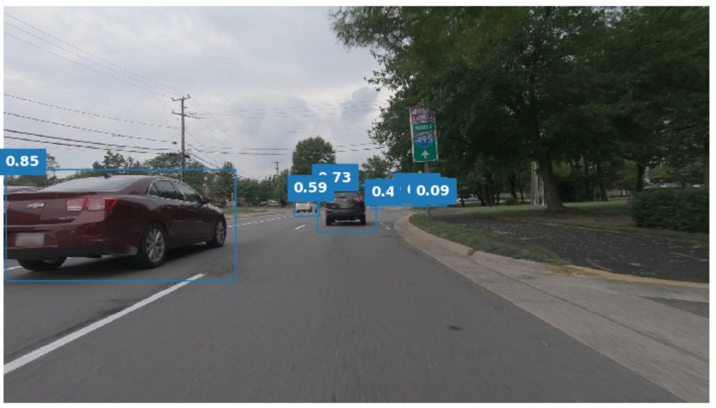
The Datadog Agent uses an API key to send monitoring data to Datadog. You can find your API key in the Datadog account settings page. Once you deploy the Agent, you can instantly access system-level metrics and visualize your infrastructure. The Agent automatically tags EC2 metrics with metadata, including Availability Zone and instance type, so you can filter, search, and group data in Datadog. For example, the Host Map helps you visualize how I/O load on d3.2xlarge instances is distributed across Availability Zones and individual instances (as shown in Figure 1 ).

Figure 1 – Visualizing read I/O operations on d3.2xlarge instances across three Availability Zones.

Figure 1 – Visualizing read I/O operations on d3.2xlarge instances across three Availability Zones.

Enabling trace collection for better visibility

Installing the Agent allows you to use Datadog APM to collect traces from the services running on your Amazon EC2 instances, and monitor their performance with Datadog dashboards and alerts.

Datadog APM includes support for auto-instrumenting applications built on a wide range of languages and frameworks, such as Java, Python, Django, and Ruby on Rails. To start collecting traces, you add the relevant Datadog tracing library to your code. For more information on setting up tracing for a specific language, Datadog has language-specific guides to help get you started.

Visualizing M5zn performance in Datadog

The new M5zn instances are a high frequency, high speed and low-latency networking variant of Amazon EC2 M5 instances. M5zn instances deliver the highest all-core turbo CPU performance from Intel Xeon Scalable processors in the cloud, with a frequency up to 4.5 GHz —making them ideal for gaming, simulation modeling, and other high performance computing applications across a broad range of industries.

To demonstrate how to visualize M5zn’s performance improvements in Datadog, we ran a benchmark test for a simple Python application deployed behind Apache servers on two instance types:

  • M5 instance (hellobench-m5-x86_64 service in Figure 2)
  • M5zn instance (hellobench-m5zn-x86_64 service in Figure 2).

Our benchmark application used the aiohttp library and was instrumented with Datadog’s Python tracing library. To run the test, we used Apache’s HTTP server benchmarking tool to generate a constant stream of requests across the two instances.

The hellobench-m5zn-x86_64 service running on the M5zn instance reported a 95th percentile latency that was about 48 percent lower than the value reported by the hellobench-m5-x86_64 service running on the M5 instance (4.73 ms vs. 9.16 ms) over the course of our testing. The summary of results is shown in Datadog APM (as shown in figure 2 below):

Figure 2 – Performance benchmarks for a Python application running on two instance types: M5 and M5zn.

Figure 2 – Performance benchmarks for a Python application running on two instance types: M5 and M5zn.

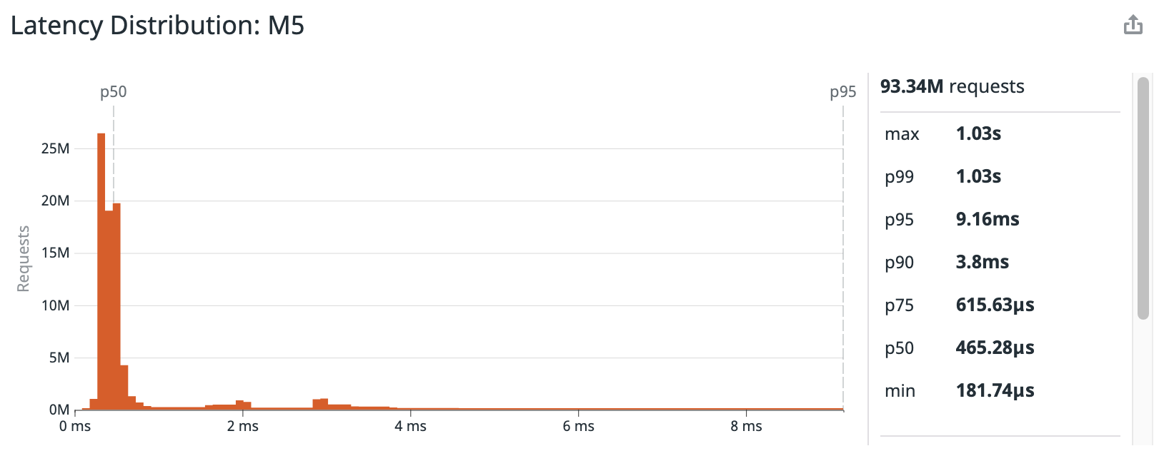
To analyze this performance data, we visualize the complete distribution of the benchmark response time results in a Datadog dashboard. Viewing the full latency distribution allows us to have a more complete picture when considering selecting the right instance type, so we can better adhere to Service Level Objective (SLO) targets.

Figure 3 shows that the M5zn was able to outperform the M5 across the entire latency distribution, both for the median request and for the long tail end of the distribution. The median request, or 50th percentile, was 36 percent faster (299.65 µs vs. 465.28 µs) while the tail end of the distribution process was 48 percent faster (4.73 ms vs. 9.16 ms) as mentioned in the preceding paragraph.


Screenshot of Latency Distribution : M5

Screenshot of Latency Distribution M5zn

Figure 3 – Using a Datadog dashboard to show how the M5zn instance type performed faster across the entire latency distribution during the benchmark test.

We can also create timeseries graphs of our test results to show that the M5zn was able to sustain faster performance throughout the duration of the test, despite processing a higher number of requests. Figure 4 illustrates the difference by displaying the 95th percentile response time and the request rate of both instances across 30-second intervals.

Figure 4 – The M5zn’s p95 latency was nearly half of the M5’s despite higher throughput during the benchmark test.

Figure 4 – The M5zn’s p95 latency was nearly half of the M5’s despite higher throughput during the benchmark test.

We can dig even deeper with Datadog Continuous Profiler, an always-on production code profiler used to analyze code-level performance across your entire environment, with minimal overhead. Profiles reveal which functions (or lines of code) consume the most resources, such as CPU and memory.

Even though M5zn is already designed to deliver excellent CPU performance, Continuous Profiler can help you optimize your applications to leverage the M5zn high-frequency processor to its maximum potential. As shown in Figure 5, the Continuous Profiler highlights lines of code where CPU utilization is exceptionally high, so you can optimize those methods or threads to make better use of the available compute power.

After you migrate your workloads to M5zn, Continuous Profiler can help you quantify CPU-time improvements on a per-method basis and pinpoint code-level bottlenecks. This also occurs even as you add new features and functionalities to your application.

Figure 5 – Using Datadog Continuous Profiler to identify functions with the most CPU time.

Figure 5 – Using Datadog Continuous Profiler to identify functions with the most CPU time.

Comparing D3, D3en, and D2 performance in Datadog

  • The new D3 and D3en instances leverage 2nd-generation Intel Xeon Scalable Processors (Cascade Lake) and provide a sustained all core frequency up to 3.1 GHz.
  • Compared to D2 instances, D3 instances provide up to 2.5x higher networking speed and 45 percent higher disk throughput.
  • D3en instances provide up to 7.5x higher networking speed, 100 percent higher disk throughput, 7x more storage capacity, and 80 percent lower cost-per-TB of storage.

These instances are ideal for HDD storage workloads, such as distributed/clustered file systems, big data and analytics, and high capacity data lakes. D3en instances are the densest local storage instances in the cloud. For our testing, we deployed the Datadog Agent to three instances: the D2, D3, and D3en. We then used two benchmark applications to gauge performance under demanding workloads.

Our first benchmark test used TestDFSIO, an open-source benchmark test included with Hadoop that is used to analyze the I/O performance of an HDFS cluster.

We ran TestDFSIO with the following command:

hadoop jar $HADOOP_HOME/share/hadoop/mapreduce/hadoop-mapreduce-client-jobclient-*-tests.jar TestDFSIO -write -nrFiles 48 -size 10GB

The Datadog Agent automatically collects system metrics that can help you visualize how the instances performed during the benchmark test. The D3en instance led the field and hit a maximum write speed of 259,000 Kbps.

Figure 6 – Using Datadog to visualize and compare write speed of an HDFS cluster on D2, D3, and D3en instance types during the TestDFSIO benchmark test.

Figure 6 – Using Datadog to visualize and compare write speed of an HDFS cluster on D2, D3, and D3en instance types during the TestDFSIO benchmark test.

The D3en instance completed the TestDFSIO benchmark test 39 percent faster than the D2 (204.55 seconds vs. 336.84 seconds). The D3 instance completed the benchmark test 27 percent faster at 244.62 seconds.

Datadog helps you realize additional benefits of the D3en and D3 instances: notably, they exhibited lower CPU utilization than the D2 during the benchmark (as shown in figure 7).

Figure 7 – Using Datadog to compare CPU usage on D2, D3, and D3en instances during the TestDFSIO benchmark test.

Figure 7 – Using Datadog to compare CPU usage on D2, D3, and D3en instances during the TestDFSIO benchmark test.

For our second benchmark test, we again deployed the Datadog Agent to the same three instances: D2, D3, and D3en. In this test, we used TPC-DS, a high CPU and I/O load test that is designed to simulate real-world database performance.

TPC-DS is a set of tools that generates a set of data that can be loaded into your database of choice, in this case PostgreSQL 12 on Ubuntu 20.04. It then generates a set of SQL statements that are used to exercise the database. For this benchmark, 8 simultaneous threads were used on each instance.

The D3en instance completed the TPC-DS benchmark test 59 percent faster than the D2 (220.31 seconds vs. 542.44 seconds). The D3 instance completed the benchmark test 53 percent faster at 253.78 seconds.

Using the metrics collected from Datadog’s PostgreSQL integration, we learn that the D3en not only finished the test faster, but had lower system load during the benchmark test run. This is further validation of the overall performance improvements you can expect when migrating to the D3en.

Figure 8 – Using Datadog to compare system load on D2, D3, and D3en instances during the TPC-DS benchmark test.

Figure 8 – Using Datadog to compare system load on D2, D3, and D3en instances during the TPC-DS benchmark test.

The performance improvements are also visible when comparing rows returned per second. While all three instances had similar peak burst performance, the D3en and D3 sustained a higher rate of rows returned throughout the duration of the TPC-DS test.

Figure 9 – Using Datadog to compare Rows returned per second on D2, D3, and D3en instances during the TPC-DS benchmark test.

Figure 9 – Using Datadog to compare Rows returned per second on D2, D3, and D3en instances during the TPC-DS benchmark test.

From these results, we learn that not only do the new D3en and D3 instances have faster disk throughput, but they also offer improved CPU performance, which translates into superior performance to power your most critical workloads.

Comparing R5b and R5 performance

The new R5b instances provide 3x higher EBS-optimized performance compared to R5 instances, and are frequently used to power large workloads that rely on Amazon EBS. Customers that operate applications with stringent storage performance requirements can consolidate their existing R5 workloads into fewer or smaller R5b instances to reduce costs.

To compare I/O performance across these two instance types, we installed the FIO benchmark application and the Datadog Agent on an R5 instance and an R5b instance. We then added EBS io1 storage volumes to each with a Provisioned IOPS setting of 25,000.

We ran FIO with a 75 percent read, 25 percent write workload using the following command:

sudo fio --randrepeat=1 --ioengine=libaio --direct=1 --gtod_reduce=1 --name=test --filename=/disk-io1/test --bs=4k --iodepth=64 --size=16G —readwrite=randrw —rwmixread=75

Using the metrics collected from the Datadog Agent, we were able to visualize the benchmark performance results. In approximately one minute, FIO ramped up and reached the maximum I/O operations per second.

The left side of Figure 10 shows the R5b instance reaching the provisioned maximum IOPS of 25,000, while the read operations at 25 percent as expected. The right side shows the R5 reaching its EBS IOPS limit of 18,750, with its relative 25 percent write operations.

It should be noted that R5b instances have far higher performance ceilings than what is being shown here, which you can find in the User Guide: Amazon EBS–optimized instances.

Figure 10 – Comparing IOPS on R5b and R5 instances during the FIO benchmark test.

Figure 10 – Comparing IOPS on R5b and R5 instances during the FIO benchmark test.

Also, note that the R5b finished the benchmark test approximately one minute faster than the R5 (166 seconds vs. 223 seconds). We learn that the shorter test duration is driven by the R5b’s faster read time, which reached a maximum of 75,000 Kbps.

Figure 11 – The R5b instance's faster read time enabled it to complete the benchmark test more quickly than the R5 instance.

Figure 11 – The R5b instance’s faster read time enabled it to complete the benchmark test more quickly than the R5 instance.

From these results, we have learned that the R5b delivers superior I/O capacity with higher throughput, making it a great choice for large relational databases and other IOPS-intensive workloads.

Conclusion

If you are thinking about shifting your workloads to one of the new Amazon EC2 instance types, you can use the Datadog Agent to immediately begin collecting and analyzing performance data. With Datadog’s other AWS integrations, you can monitor even more of your AWS infrastructure and correlate that data with the data collected by the Agent. For example, if you’re running EBS-optimized R5b instances, you can monitor them alongside performance data from your EBS volumes with Datadog’s Amazon EBS integration.

About Datadog

Datadog is an AWS Partner Network (APN) Advanced Technology Partner with AWS Competencies in DevOps, Migration, Containers, and Microsoft Workloads.

Read more about the M5zn, D3en, D3, and R5b instances, and sign up for a free Datadog trial if you don’t already have an account.

Field Notes provides hands-on technical guidance from AWS Solutions Architects, consultants, and technical account managers, based on their experiences in the field solving real-world business problems for customers.


Danton Rodriguez

Danton is a Product Manager at Datadog focused on distributed systems observability and efficiency.

Field Notes: Data-Driven Risk Analysis with Amazon Neptune and Amazon Elasticsearch Service

Post Syndicated from Adriaan de Jonge original https://aws.amazon.com/blogs/architecture/field-notes-data-driven-risk-analysis-with-amazon-neptune-and-amazon-elasticsearch-service/

This blog post is co-authored with Charles Crouspeyre and Angad Srivastava. Charles is Director at Accenture Applied Intelligence and ASEAN AI SME (Subject Matter Expert) and Angad is Data and Analytics Consultant at AWS and NLP (Natural Language Processing) expert. Together, they are the lead architects of the solution presented in this blog.

In this blog, you learn how Amazon Neptune as a graph database, combined with Amazon Elasticsearch Service (Amazon ES) for full text indexing helps you shorten risk analysis processes from weeks to minutes. We give a walk-through of the steps involved in creating this knowledge management solution, which includes natural language processing components.

The business problem

Our Energy customer needs to do a risk assessment before acquiring raw materials that will be processed in their equipment. The process includes assessing the inventory of raw materials, the capacity of storage units, analyzing the performance of the processing units, and quality assurance of the end product. The cycle time for a comprehensive risk analysis across different teams working in silos is more than 2 weeks, while the window of opportunity for purchasing is a couple of days. So, the customer either puts their equipment and personnel at risk or misses good buying opportunities.

The solution described in this blog helps our customer improve and speed up their decision making. This is done through an automated analysis and understanding of the documents and information they have gathered over the years. They use Natural Language Processing (NLP) to analyze and better understand the documents which is discussed later on in this blog.

Our customer has accumulated years of documents that were mostly in silos across the organization: emails, SharePoint, local computer, private notes, and more.

The data is so heterogenous and widespread that it became hard for our customer to retrieve the right information in a timely manner. Our objective was to create a platform centralizing all this information, and to facilitate present and future information retrieval. Making informed decisions on time helps our customer to purchase raw materials at a better price, increasing their margins significantly.

Overview of business solution

To understand the tasks involved, let’s look at the high-level platform workflow:

Figure 1: This illustration visualizes a 4-step process consisting of Hydrate, Analyze, Search and Feedback.

Figure 1: This illustration visualizes a 4-step process consisting of Hydrate, Analyze, Search and Feedback.

We can summarize our workflow as a 4-step process:

  1. Hydrate: where we extract the information from multiple sources and do a first level of processing such as document scanning and natural language processing (NLP).
  2. Analyze: where the information extracted from the hydration step is ingested and merged with existing information.
  3. Search: where information is retrieved from the system based on user queries, by leveraging our knowledge graph and the concept map representation that we have created.
  4. Feedback: where users can rate the results for the system as good or bad. The feedback is collected and used to update the Knowledge graph, to re-train our models or to improve our query matching layer.

High-level technical architecture

The following architecture consists of a traditional data layer, combined with a knowledge layer. The compute part of the solution is serverless. The database storage part requires long-running solutions.

Figure 2: A diagram visualizing the steps involved in data processing across two layers, the data layer and the knowledge layer and their implementations with AWS services.

Figure 2: A diagram visualizing the steps involved in data processing across two layers, the data layer and the knowledge layer and their implementations with AWS services.

The data layer of our application is similar to many common data analytics setups, and includes:

  • An ingestion and normalization component, implemented with AWS Lambda, fronted by Amazon API Gateway and AWS Transfer Family
  • An ETL component, implemented with AWS Glue and AWS Lambda
  • A data enhancement component, implemented with Lambda
  • An analytics component, implemented with Amazon Redshift
  • A knowledge query component, implemented with Lambda
  • A user interface, a custom implementation based on React

Where our solution really adds value, is the knowledge layer, which is what we will focus on in this blog. We created this specifically for our knowledge representation and management. This layer consists of the following:

  • The knowledge extraction block, where the raw text is extracted, analyzed and classified into facts and structured data. This is implemented using Amazon SageMaker and Amazon Comprehend.
  • The knowledge repository, where the raw data is saved and kept is Amazon Simple Storage Service (Amazon S3).
  • The relationship, and knowledge extraction, and indexing, where the facts extracted earlier are analyzed and added to our knowledge graph.  This is implemented with a combination of Neptune, Amazon S3, Amazon DocumentDB (with MongoDB compatibility) and Amazon ES. Neptune is used as a property graph, queried with the Gremlin graph traversal language.
  • The knowledge aggregator, where we leverage both our knowledge graph and business representation to extract facts to associate with the user query, and rank information based on their relevance. This is implemented leveraging Amazon ES.

The last component, the knowledge aggregator, is fundamental for our infrastructure. In general, when we talk about information retrieval system – a system designed to supply the right information in the hands of users at the right time – there are two common approaches:

  1. Keyword-based search: take the user query and search for the presence of certain keywords from the query in the available documents.
  2. Concept-based search: build a business-related taxonomy to extend the keyword-based search into a business-related concept-based search.

The downside of a keyword-based search is that it does not capture the complexity and specificity of the business domain in which the query occurs.  Due to this limitation, we chose to go with a concept-based search approach as it allows us to inject a layer of business understanding to our ingestion and information retrieval.

Knowledge layer deep-dive

Because the value added from our solution is in the knowledge layer, let’s dive deeper into the details of this layer.

Figure 3: An architecture diagram of the knowledge layer of the solution, classified in 3 categories: ingestion, knowledge representation and retrieval

Figure 3: An architecture diagram of the knowledge layer of the solution, classified in 3 categories: ingestion, knowledge representation and retrieval

The architecture in Figure 3 describes the technical solution architecture broken down into 3 key steps. The 3 steps are:

  1. Ingestion
  2. Knowledge representation
  3. Retrieval

Another way to approach the problem definition is by looking at the process flow for how raw data/information flows through the system to generate the knowledge layer. Figure 4 gives an example of how the information is broadly treated as it progresses the logical phases of the process flow.


Figure 6: Context based Knowledge Graph Generation

Figure 4: An illustration of how information is extracted from an unstructured document, modeled as a graph and visualized in a business-friendly and concise format.

In this example, we can recognize a raw material of type “Champion” and detect a relationship between this entity and another entity of type “basic nitrogen”. This relationship is classified as the type “is characterized by”.

The facts in the parsed content are then classified into different categories of relevancy based on the contextual information contained in the text i.e., an important paragraph that mentions a potential issue will get classified as a key highlight with a high degree of relevancy.

This paragraph text is further analyzed to recognize and extract entities mentioned such as “Champion” and “basic nitrogen”; and to determine the semantic relationship between these entities based on the context of the paragraph i.e., “characterized by” and, “incompatibility due to low levels of basic nitrogen”.

There is a correlation between the different steps of the technical architecture versus the phases in the information analysis process. So we will present them together.

This table shows the correlation between the different steps of the technical architecture versus the phases in the information analysis process.

  • During the Ingestion step in the technical solution architecture, the aim is to process the incoming raw data in any format as defined in the Extract Information phase of the information analysis process flow.
  • Once the data ingestion has occurred, the next step is to capture the knowledge representation. The contextualize information phase of the information analysis process flow helps ensure that comprehensive and accurate knowledge representation occurs within the system.
  • The last step for the solution is to then facilitate retrieval of information by providing appropriate interfaces for interacting with the knowledge representation within the system. This is facilitated by the assemble information phase of the Information Analysis process.

To further understand the proposed solution, let us review the steps and the associated process flow phases.

Technical Architecture Step 1: Ingestion

Information comes in through the ingestion pipeline from various sources, such as websites, reports, news, blogs and internal data. Raw data enters the system either through automated API-based integrations with external websites or internal systems like Microsoft SharePoint, or can be ingested manually through AWS Transfer Family. Once a new piece of data has been ingested into the solution, it initiates the process for extracting information from the raw data.

Information Analysis Phase 1: Extract information

Once the information lands in our system, the knowledge representation process starts with our Lambda functions acting as the orchestrator between other components. Amazon SageMaker was initially used to create custom models for document categorization and classification of ingested unstructured files.

For example, an unstructured file that is ingested into our system gets recognized as a new email (one of the acceptable data sources) and is classified as “compatibility highlights” based on the email contents. But with improvements in the capabilities of Amazon Comprehend managed service, the need for custom model development, maintenance, and machine learning operations (MLOps) could be reduced. The solution now uses Amazon Comprehend with custom training for the initial step of document categorization and information extraction. Additionally, Amazon Comprehend was also used to create custom named-entity recognition models, that were trained to recognize custom raw materials and properties.

In this example, an unstructured pdf document is ingested into our system as illustrated in Figure 5.

Example of an unstructured pdf document being ingested into our system

Figure 5: Phase 1 – Information Extraction

Amazon Comprehend analyzes the unstructured document, classifies its contents and extracts a specific piece of information regarding a type of raw material called “Champion”. This has an inherent property called “low basic nitrogen” associated with it.

Technical Architecture Step 2: Knowledge representation

Knowledge representation is the process of extracting semantic relationships between the various information/data elements within a piece of raw data. It then incorporates it into the existing layers of knowledge already identified and stored. Based on the categorization of the document, the raw text is pre-processed and parsed into logical units. The parsed data is then analyzed in our NLP layer for content identification and fact classification.

The facts and key relationships deduced from the results of both Amazon Comprehend are returned back to the Lambda functions, which in-turn store the detected facts to the knowledge graph.

Information Analysis Phase 2: Contextualize information

Once the information is extracted from the document; our first step is to contextualize the information using our business representation in the form of a taxonomy. The system detects different parts and entities that the paragraph is composed of, and structures the information into our knowledge graph as illustrated in Figure 6.

Figure 6: Context based Knowledge Graph Generation

Figure 6: Context based Knowledge Graph Generation

This data extraction process is repeated iteratively, so that the knowledge graph grows over time through the detection of new facts and relationships. When we ingest new data into our knowledge graph, we search our knowledge graph for similar entities. If a similar entity exists, we analyze the type of relationships and properties both entities have. When we observe sufficient similarities between the entities, we associate relationships from one entity to the other.

For example, a new entity “Crude A” which has the properties – level of basic nitrogen and level of sulfur is ingested. Next, we have “Champion”, as described above, which has similar levels of basic nitrogen and a property “risk” associated to it. Based on the existing knowledge graph, we can now infer that there is a high probability that “Crude A” has a similar risk associated to it as shown in Figure 7.

Figure 7: Crude Knowledge Graph Representation

Figure 7: Crude Knowledge Graph Representation

The probability calculations can take multiple factors into consideration to make the process more accurate. This makes the structure of the knowledge graph quite dynamic and evolve automatically.

The complete raw data is also stored in Amazon ES as a secondary implementation to perform free form queries. This process helps ensure that all the relevant information for any extracted factoid associated with an entity in the knowledge graph is completely represented with the system. Some of this information may not exist in the knowledge graph because the document data extraction model can’t capture all the relevant information. One reason for such a problem to occur can be poor quality of the source document making automated reading of documents and data extraction difficult. Another reason can be the sophistication of the Amazon Comprehend models.

Technical Architecture Step 3: Retrieval

To retrieve information, the user query is analyzed by the Lambda function on the right side of Figure 3. Based on the analysis, key terms are identified from the user query for which a search needs to be performed. For example, if the query provided is “What is the likelihood of damage due to processing Champion in location A”, semantic analysis of the query will indicate that we are looking for relationships between entities Champion, any type of risks, any known incidents at location A and possible mitigations to reduce identified risks.

To address the query, the information then needs to compiled together from the existing knowledge graph as well as Amazon ES to provide a complete answer.

Information Analysis Phase 3: Assemble information

Figure 8 illustrates the output of Information assembly process.

Figure 8: "Champion" crude assembled information for property Nitrogen

Figure 8: “Champion” crude assembled information for property Nitrogen

Based on the facts available within the knowledge graph, we have identified that for “Champion” there is a possibility of damage occurring “due to increased pressure drop and loss of heat transfer” but this can be mitigated by “blending champion to meet basic nitrogen levels”.

In addition, say there was information available about “Crude B” that has been processed at “location A”. This also originated from “Brunei” and had similar “Nitrogen” and properties such as “Kerogen3”, “napthenic” and had a processing incident causing damage. We can then conclude by looking at the information stored within the knowledge graph and Amazon ES, that there are other possibilities for damage to occur due to processing of “Champion” at “Location A” as well.

Once all the relevant pieces of information have been collected, a sorted list of information is sent back to the user interface to be displayed.

Fact reconciliation

In reality, it is possible that new information contradicts existing information, which causes conflicts during ingestion. There are various ways to handle such contradictions, for example:

Figure 5: Visualizations of four illustrative ways to deal with contradictory new facts.

Figure 9: Visualizations of four illustrative ways to deal with contradictory new facts.

  1. Assume the latest data is the most accurate, by looking at the timestamp of each data point. This makes it possible to update the list of facts in our knowledge graph
  2. Analyze how new facts alter the properties or relationships of existing facts and update them or create a relationship between nodes
  3. Calculate a reliability score for the available sources, to rank the fact based on who has provided them
  4. Ask for end user feedback through the user interface

In our solution, we have mechanism 1, 2, and 4. Mechanisms 1 and 2 are implemented within the contextualize information phase of the information analysis process.

Mechanism 4 is implemented in the search results use interface where the user has a ‘thumbs up’ and ‘thumbs down’ button to classify the different search results as relevant or not. This information is then fed back into the Amazon Comprehend model, the knowledge graph as well as captured within Amazon ES to optimize subsequent search results.

Over time, mechanism 4 can be expanded to capture more detailed feedback including corrections to the search result instead of a simple yes/no feedback mechanism.  Such enhancements to mechanism 4 and the implementation of Mechanism 3 can be a possible future enhancement for the solution proposed.

Conclusion

Our customer needed help to shorten their risk analysis process to make high-impact purchase decisions for raw materials. Our knowledge management solution helped them extract knowledge from their vast set of documents and make it available in knowledge graph format, for risk analysts to analyze. Knowledge graphs are a great way to handle this “domain specificity”. It helps extract information during the ingestion phase. It also helps contextualize queries during the retrieval phase.

The possibilities are endless. One thing is certain: we’d encourage you to use graph databases with Neptune supported by Amazon ES for your use cases with highly connected data!

Field Notes provides hands-on technical guidance from AWS Solutions Architects, consultants, and technical account managers, based on their experiences in the field solving real-world business problems for customers.


Charles Crouspeyre

Charles Crouspeyre is leading the AI Engineering practice for Accenture in ASEAN, where he is helping companies from all industries think and deploy their AI ambitions. When not working, he likes to spend time with his young-aged daughter reading/drawing/cooking/singing/playing hide & seek with her as she “requests”.

Angad Srivastava

Angad Srivastava

Angad Srivastava is a Data and Analytics Consultant at AWS in Singapore, where he consults with clients in ASEAN to develop robust AI solutions. When not at his desk, he can be found planning his next budget-friendly backpacking trip to check off yet another country from his bucket list.

Field Notes: Accelerate Research with Managed Jupyter on Amazon SageMaker

Post Syndicated from Mrudhula Balasubramanyan original https://aws.amazon.com/blogs/architecture/field-notes-accelerate-research-with-managed-jupyter-on-amazon-sagemaker/

Research organizations across industry verticals have unique needs. These include facilitating stakeholder collaboration, setting up compute environments for experimentation, handling large datasets, and more. In essence, researchers want the freedom to focus on their research, without the undifferentiated heavy-lifting of managing their environments.

In this blog, I show you how to set up a managed Jupyter environment using custom tools used in Life Sciences research. I show you how to transform the developed artifacts into scripted components that can be integrated into research workflows. Although this solution uses Life Sciences as an example, it is broadly applicable to any vertical that needs customizable managed environments at scale.

Overview of solution

This solution has two parts. First, the System administrator of an organization’s IT department sets up a managed environment and provides researchers access to it. Second, the researchers access the environment and conduct interactive and scripted analysis.

This solution uses AWS Single Sign-On (AWS SSO), Amazon SageMaker, Amazon ECR, and Amazon S3. These services are architected to build a custom environment, provision compute, conduct interactive analysis, and automate the launch of scripts.

Walkthrough

The architecture and detailed walkthrough are presented from both an admin and researcher perspective.

Architecture from an admin perspective

Architecture from admin perspective


In order of tasks, the admin:

  1. authenticates into AWS account as an AWS Identity and Access Management (IAM) user with admin privileges
  2. sets up AWS SSO and users who need access to Amazon SageMaker Studio
  3. creates a Studio domain
  4. assigns users and groups created in AWS SSO to the Studio domain
  5. creates a SageMaker notebook instance shown generically in the architecture as Amazon EC2
  6. launches a shell script provided later in this post to build and store custom Docker image in a private repository in Amazon ECR
  7. attaches the custom image to Studio domain that the researchers will later use as a custom Jupyter kernel inside Studio and as a container for the SageMaker processing job.

Architecture from a researcher perspective

Architecture from a researcher perspective

In order of tasks, the researcher:

  1. authenticates using AWS SSO
  2. SSO authenticates researcher to SageMaker Studio
  3. researcher performs interactive analysis using managed Jupyter notebooks with custom kernel, organizes the analysis into script(s), and launches a SageMaker processing job to execute the script in a managed environment
  4. the SageMaker processing job reads data from S3 bucket and writes data back to S3. The user can now retrieve and examine results from S3 using Jupyter notebook.

Prerequisites

For this walkthrough, you should have:

  • An AWS account
  • Admin access to provision and delete AWS resources
  • Researchers’ information to add as SSO users: full name and email

Set up AWS SSO

To facilitate collaboration between researchers, internal and external to your organization, the admin uses AWS SSO to onboard to Studio.

For admins: follow these instructions to set up AWS SSO prior to creating the Studio domain.

Onboard to SageMaker Studio

Researchers can use just the functionality they need in Amazon SageMaker Studio. Studio provides managed Jupyter environments with sharable notebooks for interactive analysis, and managed environments for script execution.

When you onboard to Studio, a home directory is created for you on Amazon Elastic File System (Amazon EFS) which provides reliable, scalable storage for large datasets.

Once AWS SSO has been setup, follow these steps to onboard to Studio via SSO. Note the Studio domain id (ex. d-2hxa6eb47hdc) and the IAM execution role (ex. AmazonSageMaker-ExecutionRole-20201156T214222) in the Studio Summary section of Studio. You will be using these in the following sections.

Provision custom image

At the core of research is experimentation. This often requires setting up playgrounds with custom tools to test out ideas. Docker images are an effective[CE1] [BM2]  way to package those tools and dependencies and deploy them quickly. They also address another critical need for researchers – reproducibility.

To demonstrate this, I picked a Life Sciences research problem that requires custom Python packages to be installed and made available to a team of researchers as Jupyter kernels inside Studio.

For the custom Docker image, I picked a Python package called Pegasus. This is a tool used in genomics research for analyzing transcriptomes of millions of single cells, both interactively as well as in cloud-based analysis workflows.

In addition to Python, you can provision Jupyter kernels for languages such as R, Scala, Julia, in Studio using these Docker images.

Launch an Amazon SageMaker notebook instance

To build and push custom Docker images to ECR, you use an Amazon SageMaker notebook instance. Note that this is not part of SageMaker Studio and unrelated to Studio notebooks. It is a fully managed machine learning (ML) Amazon EC2 instance inside the SageMaker service that runs the Jupyter Notebook application, AWS CLI, and Docker.

  • Use these instructions to launch a SageMaker notebook instance.
  • Once the notebook instance is up and running, select the instance and navigate to the IAM role attached to it. This role comes with IAM policy ‘AmazonSageMakerFullAccess’ as a default. Your instance will need some additional permissions.
  • Create a new IAM policy using these instructions.
  • Copy the IAM policy below to paste into the JSON tab.
  • Fill in the values for <region-id> (ex. us-west-2), <AWS-account-id>, <studio-domain-id>, <studio-domain-iam-role>. Name the IAM policy ‘sagemaker-notebook-policy’ and attach it to the notebook instance role.
{
    "Version": "2012-10-17",
    "Statement": [
        {
            "Sid": "additionalpermissions",
            "Effect": "Allow",
            "Action": [
                "iam:PassRole",
                "sagemaker:UpdateDomain"
            ],
            "Resource": [
                "arn:aws:sagemaker:<region-id>:<AWS-account-id>:domain/<studio-domain-id>",
                "arn:aws:iam::<AWS-account-id>:role/<studio-domain-iam-role>"
            ]
        }
    ]
}
  • Start a terminal session in the notebook instance.
  • Once you are done creating the Docker image and attaching to Studio in the next section, you will be shutting down the notebook instance.

Create private repository, build, and store custom image, attach to SageMaker Studio domain

This section has multiple steps, all of which are outlined in a single bash script.

  • First the script creates a private repository in Amazon ECR.
  • Next, the script builds a custom image, tags, and pushes to Amazon ECR repository. This custom image will serve two purposes: one as a custom Python Jupyter kernel used inside Studio, and two as a custom container for SageMaker processing.
  • To use as a custom kernel inside SageMaker Studio, the script creates a SageMaker image and attaches to the Studio domain.
  • Before you initiate the script, fill in the following information: your AWS account ID, Region (ex. us-east-1), Studio IAM execution role, and Studio domain id.
  • You must create four files: bash script, Dockerfile, and two configuration files.
  • Copy the following bash script to a file named ‘pegasus-docker-images.sh’ and fill in the required values.
#!/bin/bash

# Pegasus python packages from Docker hub

accountid=<fill-in-account-id>

region=<fill-in-region>

executionrole=<fill-in-execution-role ex. AmazonSageMaker-ExecutionRole-xxxxx>

domainid=<fill-in-Studio-domain-id ex. d-xxxxxxx>

if aws ecr describe-repositories | grep 'sagemaker-custom'
then
    echo 'repo already exists! Skipping creation'
else
    aws ecr create-repository --repository-name sagemaker-custom
fi

aws ecr get-login-password --region $region | docker login --username AWS --password-stdin $accountid.dkr.ecr.$region.amazonaws.com

docker build -t sagemaker-custom:pegasus-1.0 .

docker tag sagemaker-custom:pegasus-1.0 $accountid.dkr.ecr.$region.amazonaws.com/sagemaker-custom:pegasus-1.0

docker push $accountid.dkr.ecr.$region.amazonaws.com/sagemaker-custom:pegasus-1.0

if aws sagemaker list-images | grep 'pegasus-1'
then
    echo 'Image already exists! Skipping creation'
else
    aws sagemaker create-image --image-name pegasus-1 --role-arn arn:aws:iam::$accountid:role/service-role/$executionrole
    aws sagemaker create-image-version --image-name pegasus-1 --base-image $accountid.dkr.ecr.$region.amazonaws.com/sagemaker-custom:pegasus-1.0
fi

if aws sagemaker list-app-image-configs | grep 'pegasus-1-config'
then
    echo 'Image config already exists! Skipping creation'
else
   aws sagemaker create-app-image-config --cli-input-json file://app-image-config-input.json
fi

aws sagemaker update-domain --domain-id $domainid --cli-input-json file://default-user-settings.json

Copy the following to a file named ‘Dockerfile’.

FROM cumulusprod/pegasus-terra:1.0

USER root

Copy the following to a file named ‘app-image-config-input.json’.

{
    "AppImageConfigName": "pegasus-1-config",
    "KernelGatewayImageConfig": {
        "KernelSpecs": [
            {
                "Name": "python3",
                "DisplayName": "Pegasus 1.0"
            }
        ],
        "FileSystemConfig": {
            "MountPath": "/root",
            "DefaultUid": 0,
            "DefaultGid": 0
        }
    }
}

Copy the following to a file named ‘default-user-settings.json’.

{
    "DefaultUserSettings": {
        "KernelGatewayAppSettings": { 
           "CustomImages": [ 
              { 
                 "ImageName": "pegasus-1",
                 "ImageVersionNumber": 1,
                 "AppImageConfigName": "pegasus-1-config"
              }
           ]
        }
    }
}

Launch ‘pegasus-docker-images.sh’ in the directory with all four files, in the terminal of the notebook instance. If the script ran successfully, you should see the custom image attached to the Studio domain.

Amazon SageMaker dashboard


Perform interactive analysis

You can now launch the Pegasus Python kernel inside SageMaker . If this is your first time using Studio, you can get a quick tour of its UI.

For interactive analysis, you can use publicly available notebooks in Pegasus tutorial from this GitHub repository. Review the license before proceeding.

To clone the repository in Studio, open a system terminal using these instructions. Initiate $ git clone https://github.com/klarman-cell-observatory/pegasus

  • In the directory ‘pegasus’, select ‘notebooks’ and open ‘pegasus_analysis.ipynb’.
  • For kernel choose ‘Pegasus 1.0 (pegasus-1/1)’.
  • You can now run through the notebook and examine the output generated. Feel free to work through the other notebooks for deeper analysis.

Pagasus tutorial

At any point during experimentation, you can share your analysis along with results with your colleagues using these steps. The snapshot that you create also captures the notebook configuration such as instance type and kernel, to ensure reproducibility.

Formalize analysis and execute scripts

Once you are done with interactive analysis, you can consolidate your analysis into a script to launch in a managed environment. This is an important step, if you want to later incorporate this script as a component into a research workflow and automate it.

Copy the following script to a file named ‘pegasus_script.py’.

"""
BSD 3-Clause License

Copyright (c) 2018, Broad Institute
All rights reserved.

Redistribution and use in source and binary forms, with or without
modification, are permitted provided that the following conditions are met:

* Redistributions of source code must retain the above copyright notice, this
  list of conditions and the following disclaimer.

* Redistributions in binary form must reproduce the above copyright notice,
  this list of conditions and the following disclaimer in the documentation
  and/or other materials provided with the distribution.

* Neither the name of the copyright holder nor the names of its
  contributors may be used to endorse or promote products derived from
  this software without specific prior written permission.

THIS SOFTWARE IS PROVIDED BY THE COPYRIGHT HOLDERS AND CONTRIBUTORS "AS IS"
AND ANY EXPRESS OR IMPLIED WARRANTIES, INCLUDING, BUT NOT LIMITED TO, THE
IMPLIED WARRANTIES OF MERCHANTABILITY AND FITNESS FOR A PARTICULAR PURPOSE ARE
DISCLAIMED. IN NO EVENT SHALL THE COPYRIGHT HOLDER OR CONTRIBUTORS BE LIABLE
FOR ANY DIRECT, INDIRECT, INCIDENTAL, SPECIAL, EXEMPLARY, OR CONSEQUENTIAL
DAMAGES (INCLUDING, BUT NOT LIMITED TO, PROCUREMENT OF SUBSTITUTE GOODS OR
SERVICES; LOSS OF USE, DATA, OR PROFITS; OR BUSINESS INTERRUPTION) HOWEVER
CAUSED AND ON ANY THEORY OF LIABILITY, WHETHER IN CONTRACT, STRICT LIABILITY,
OR TORT (INCLUDING NEGLIGENCE OR OTHERWISE) ARISING IN ANY WAY OUT OF THE USE
OF THIS SOFTWARE, EVEN IF ADVISED OF THE POSSIBILITY OF SUCH DAMAGE.

"""

import pandas as pd
import pegasus as pg

if __name__ == "__main__":
    BASE_DIR = "/opt/ml/processing"
    data = pg.read_input(f"{BASE_DIR}/input/MantonBM_nonmix_subset.zarr.zip")
    pg.qc_metrics(data, percent_mito=10)
    df_qc = pg.get_filter_stats(data)
    pd.DataFrame(df_qc).to_csv(f"{BASE_DIR}/output/qc_metrics.csv", header=True, index=False)

The Jupyter notebook following provides an example of launching a processing job using the script in SageMaker.

  • Create a notebook in SageMaker Studio in the same directory as the script.
  • Copy the following code to the notebook and name it ‘sagemaker_pegasus_processing.ipynb’.
  • Select ‘Python 3 (Data Science)’ as the kernel.
  • Launch the cells.
import boto3
import sagemaker
from sagemaker import get_execution_role
from sagemaker.processing import ScriptProcessor, ProcessingInput, ProcessingOutput
region = boto3.Session().region_name
sagemaker_session = sagemaker.session.Session()
role = sagemaker.get_execution_role()
bucket = sagemaker_session.default_bucket()

prefix = 'pegasus'

account_id = boto3.client('sts').get_caller_identity().get('Account')
ecr_repository = 'research-custom'
tag = ':pegasus-1.0'

uri_suffix = 'amazonaws.com'
if region in ['cn-north-1', 'cn-northwest-1']:
    uri_suffix = 'amazonaws.com.cn'
processing_repository_uri = '{}.dkr.ecr.{}.{}/{}'.format(account_id, region, uri_suffix, ecr_repository + tag)
print(processing_repository_uri)

script_processor = ScriptProcessor(command=['python3'],
                image_uri=processing_repository_uri,
                role=role,
                instance_count=1,
                instance_type='ml.m5.xlarge')
!wget https://storage.googleapis.com/terra-featured-workspaces/Cumulus/MantonBM_nonmix_subset.zarr.zip

local_path = "MantonBM_nonmix_subset.zarr.zip"

s3 = boto3.resource("s3")

base_uri = f"s3://{bucket}/{prefix}"
input_data_uri = sagemaker.s3.S3Uploader.upload(
    local_path=local_path, 
    desired_s3_uri=base_uri,
)
print(input_data_uri)

code_uri = sagemaker.s3.S3Uploader.upload(
    local_path="pegasus_script.py", 
    desired_s3_uri=base_uri,
)
print(code_uri)

script_processor.run(code=code_uri,
                      inputs=[ProcessingInput(source=input_data_uri, destination='/opt/ml/processing/input'),],
                      outputs=[ProcessingOutput(source="/opt/ml/processing/output", destination=f"{base_uri}/output")]
                     )
script_processor_job_description = script_processor.jobs[-1].describe()
print(script_processor_job_description)

output_path = f"{base_uri}/output"
print(output_path)

The ‘output_path’ is the S3 prefix where you will find the results from SageMaker processing. This will be printed as the last line after execution. You can examine the results either directly in S3 or by copying the results back to your home directory in Studio.

Cleaning up

To avoid incurring future charges, shut down the SageMaker notebook instance. Detach image from the Studio domain, delete image in Amazon ECR, and delete data in Amazon S3.

Conclusion

In this blog, I showed you how to set up and use a unified research environment using Amazon SageMaker. Although the example pertained to Life Sciences, the architecture and the framework presented are generally applicable to any research space. They strive to address the broader research challenges of custom tooling, reproducibility, large datasets, and price predictability.

As a logical next step, take the scripted components and incorporate them into research workflows and automate them. You can use SageMaker Pipelines to incorporate machine learning into your workflows and operationalize them.

Field Notes provides hands-on technical guidance from AWS Solutions Architects, consultants, and technical account managers, based on their experiences in the field solving real-world business problems for customers.

Field Notes: Enroll Existing AWS Accounts into AWS Control Tower

Post Syndicated from Kishore Vinjam original https://aws.amazon.com/blogs/architecture/field-notes-enroll-existing-aws-accounts-into-aws-control-tower/

Originally published 21 April 2020 to the Field Notes blog, and updated in August 2020 with new prechecks to the account enrollment script. 

Since the launch of AWS Control Tower, customers have been asking for the ability to deploy AWS Control Tower in their existing AWS Organizations and to extend governance to those accounts in their organization.

We are happy that you can now deploy AWS Control Tower in your existing AWS Organizations. The accounts that you launched before deploying AWS Control Tower, what we refer to as unenrolled accounts, remain outside AWS Control Towers’ governance by default. These accounts must be enrolled in the AWS Control Tower explicitly.

When you enroll an account into AWS Control Tower, it deploys baselines and additional guardrails to enable continuous governance on your existing AWS accounts. However, you must perform proper due diligence before enrolling in an account. Refer to the Things to Consider section below for additional information.

In this blog, I show you how to enroll your existing AWS accounts and accounts within the unregistered OUs in your AWS organization under AWS Control Tower programmatically.

Background

Here’s a quick review of some terms used in this post:

  • The Python script provided in this post. This script interacts with multiple AWS services, to identify, validate, and enroll the existing unmanaged accounts into AWS Control Tower.
  • An unregistered organizational unit (OU) is created through AWS Organizations. AWS Control Tower does not manage this OU.
  • An unenrolled account is an existing AWS account that was created outside of AWS Control Tower. It is not managed by AWS Control Tower.
  • A registered organizational unit (OU) is an OU that was created in the AWS Control Tower service. It is managed by AWS Control Tower.
  • When an OU is registered with AWS Control Tower, it means that specific baselines and guardrails are applied to that OU and all of its accounts.
  • An AWS Account Factory account is an AWS account provisioned using account factory in AWS Control Tower.
  • Amazon Elastic Compute Cloud (Amazon EC2) is a web service that provides secure, resizable compute capacity in the cloud.
  • AWS Service Catalog allows you to centrally manage commonly deployed IT services. In the context of this blog, account factory uses AWS Service Catalog to provision new AWS accounts.
  • AWS Organizations helps you centrally govern your environment as you grow and scale your workloads on AWS.
  • AWS Single Sign-On (SSO) makes it easy to centrally manage access to multiple AWS accounts. It also provides users with single sign-on access to all their assigned accounts from one place.

Things to Consider

Enrolling an existing AWS account into AWS Control Tower involves moving an unenrolled account into a registered OU. The Python script provided in this blog allows you to enroll your existing AWS accounts into AWS Control Tower. However, it doesn’t have much context around what resources are running on these accounts. It assumes that you validated the account services before running this script to enroll the account.

Some guidelines to check before you decide to enroll the accounts into AWS Control Tower.

  1. An AWSControlTowerExecution role must be created in each account. If you are using the script provided in this solution, it creates the role automatically for you.
  2. If you have a default VPC in the account, the enrollment process tries to delete it. If any resources are present in the VPC, the account enrollment fails.
  3. If AWS Config was ever enabled on the account you enroll, a default config recorder and delivery channel were created. Delete the configuration-recorder and delivery channel for the account enrollment to work.
  4. Start with enrolling the dev/staging accounts to get a better understanding of any dependencies or impact of enrolling the accounts in your environment.
  5. Create a new Organizational Unit in AWS Control Tower and do not enable any additional guardrails until you enroll in the accounts. You can then enable guardrails one by one to check the impact of the guardrails in your environment.
  6. As an additional option, you can apply AWS Control Tower’s detective guardrails to an existing AWS account before moving them under Control Tower governance. Instructions to apply the guardrails are discussed in detail in AWS Control Tower Detective Guardrails as an AWS Config Conformance Pack blog.

Prerequisites

Before you enroll your existing AWS account in to AWS Control Tower, check the prerequisites from AWS Control Tower documentation.

This Python script provided part of this blog, supports enrolling all accounts with in an unregistered OU in to AWS Control Tower. The script also supports enrolling a single account using both email address or account-id of an unenrolled account. Following are a few additional points to be aware of about this solution.

  • Enable trust access with AWS Organizations for AWS CloudFormation StackSets.
  • The email address associated with the AWS account is used as AWS SSO user name with default First Name Admin and Last Name User.
  • Accounts that are in the root of the AWS Organizations can be enrolled one at a time only.
  • While enrolling an entire OU using this script, the AWSControlTowerExecution role is automatically created on all the accounts on this OU.
  • You can enroll a single account with in an unregistered OU using the script. It checks for AWSControlTowerExecution role on the account. If the role doesn’t exist, the role is created on all accounts within the OU.
  • By default, you are not allowed to enroll an account that is in the root of the organization. You must pass an additional flag to launch a role creation stack set across the organization
  • While enrolling a single account that is in the root of the organization, it prompts for additional flag to launch role creation stack set across the organization.
  • The script uses CloudFormation Stack Set Service-Managed Permissions to create the AWSControlTowerExecution role in the unenrolled accounts.

How it works

The following diagram shows the overview of the solution.

Account enrollment

  1. In your AWS Control Tower environment, access an Amazon EC2 instance running in the master account of the AWS Control Tower home Region.
  2. Get temporary credentials for AWSAdministratorAccess from AWS SSO login screen
  3. Download and execute the enroll_script.py script
  4. The script creates the AWSControlTowerExecution role on the target account using Automatic Deployments for a Stack Set feature.
  5. On successful validation of role and organizational units that are given as input, the script launches a new product in Account Factory.
  6. The enrollment process creates an AWS SSO user using the same email address as the AWS account.

Setting up the environment

It takes up to 30 minutes to enroll each AWS account in to AWS Control Tower. The accounts can be enrolled only one at a time. Depending on number of accounts that you are migrating, you must keep the session open long enough. In this section, you see one way of keeping these long running jobs uninterrupted using Amazon EC2 using the screen tool.

Optionally you may use your own compute environment where the session timeouts can be handled. If you go with your own environment, make sure you have python3, screen and a latest version of boto3 installed.

1. Prepare your compute environment:

  • Log in to your AWS Control Tower with AWSAdministratorAccess role.
  • Switch to the Region where you deployed your AWS Control Tower if needed.
  • If necessary, launch a VPC using the stack here and wait for the stack to COMPLETE.
  • If necessary, launch an Amazon EC2 instance using the stack here. Wait for the stack to COMPLETE.
  • While you are on master account, increase the session time duration for AWS SSO as needed. Default is 1 hour and maximum is 12 hours.

2. Connect to the compute environment (one-way):

  • Go to the EC2 Dashboard, and choose Running Instances.
  • Select the EC2 instance that you just created and choose Connect.
  • In Connect to your instance screen, under Connection method, choose EC2InstanceConnect (browser-based SSH connection) and Connect to open a session.
  • Go to AWS Single Sign-On page in your browser. Click on your master account.
  • Choose command line or programmatic access next to AWSAdministratorAccess.
  • From Option 1 copy the environment variables and paste them in to your EC2 terminal screen in step 5 below.

3. Install required packages and variables. You may skip this step, if you used the stack provided in step-1 to launch a new EC2 instance:

  • Install python3 and boto3 on your EC2 instance. You may have to update boto3, if you use your own environment.
$ sudo yum install python3 -y 
$ sudo pip3 install boto3
$ pip3 show boto3
Name: boto3
Version: 1.12.39
  • Change to home directory and download the enroll_account.py script.
$ cd ~
$ wget https://raw.githubusercontent.com/aws-samples/aws-control-tower-reference-architectures/master/customizations/AccountFactory/EnrollAccount/enroll_account.py
  • Set up your home Region on your EC2 terminal.
export AWS_DEFAULT_REGION=<AWSControlTower-Home-Region>

4. Start a screen session in daemon mode. If your session gets timed out, you can open a new session and attach back to the screen.

$ screen -dmS SAM
$ screen -ls
There is a screen on:
        585.SAM (Detached)
1 Socket in /var/run/screen/S-ssm-user.
$ screen -dr 585.SAM 

5. On the screen terminal, paste the environmental variable that you noted down in step 2.

6. Identify the accounts or the unregistered OUs to migrate and run the Python script provide with below mentioned options.

  • Python script usage:
usage: enroll_account.py -o -u|-e|-i -c 
Enroll existing accounts to AWS Control Tower.

optional arguments:
  -h, --help            show this help message and exit
  -o OU, --ou OU        Target Registered OU
  -u UNOU, --unou UNOU  Origin UnRegistered OU
  -e EMAIL, --email EMAIL
                        AWS account email address to enroll in to AWS Control Tower
  -i AID, --aid AID     AWS account ID to enroll in to AWS Control Tower
  -c, --create_role     Create Roles on Root Level
  • Enroll all the accounts from an unregistered OU to a registered OU
$ python3 enroll_account.py -o MigrateToRegisteredOU -u FromUnregisteredOU 
Creating cross-account role on 222233334444, wait 30 sec: RUNNING 
Executing on AWS Account: 570395911111, [email protected] 
Launching Enroll-Account-vinjak-unmgd3 
Status: UNDER_CHANGE. Waiting for 6.0 min to check back the Status 
Status: UNDER_CHANGE. Waiting for 5.0 min to check back the Status 
. . 
Status: UNDER_CHANGE. Waiting for 1.0 min to check back the Status 
SUCCESS: 111122223333 updated Launching Enroll-Account-vinjakSCchild 
Status: UNDER_CHANGE. Waiting for 6.0 min to check back the Status 
ERROR: 444455556666 
Launching Enroll-Account-Vinjak-Unmgd2 
Status: UNDER_CHANGE. Waiting for 6.0 min to check back the Status 
. . 
Status: UNDER_CHANGE. Waiting for 1.0 min to check back the Status 
SUCCESS: 777788889999 updated
  • Use AWS account ID to enroll a single account that is part of an unregistered OU.
$ python3 enroll_account.py -o MigrateToRegisteredOU -i 111122223333
  • Use AWS account email address to enroll a single account from an unregistered OU.
$ python3 enroll_account.py -o MigrateToRegisteredOU -e [email protected]

You are not allowed by default to enroll an AWS account that is in the root of the organization. The script checks for the AWSControlTowerExecution role in the account. If role doesn’t exist, you are prompted to use -c | --create-role. Using -c flag adds the stack instance to the parent organization root. Which means an AWSControlTowerExecution role is created in all the accounts with in the organization.

Note: Ensure installing AWSControlTowerExecution role in all your accounts in the organization, is acceptable in your organization before using -c flag.

If you are unsure about this, follow the instructions in the documentation and create the AWSControlTowerExecution role manually in each account you want to migrate. Rerun the script.

  • Use AWS account ID to enroll a single account that is in root OU (need -c flag).
$ python3 enroll_account.py -o MigrateToRegisteredOU -i 111122223333 -c
  • Use AWS account email address to enroll a single account that is in root OU (need -c flag).
$ python3 enroll_account.py -o MigrateToRegisteredOU -e [email protected] -c

Cleanup steps

On successful completion of enrolling all the accounts into your AWS Control Tower environment, you could clean up the below resources used for this solution.

If you have used templates provided in this blog to launch VPC and EC2 instance, delete the EC2 CloudFormation stack and then VPC template.

Conclusion

Now you can deploy AWS Control Tower in an existing AWS Organization. In this post, I have shown you how to enroll your existing AWS accounts in your AWS Organization into AWS Control Tower environment. By using the procedure in this post, you can programmatically enroll a single account or all the accounts within an organizational unit into an AWS Control Tower environment.

Now that governance has been extended to these accounts, you can also provision new AWS accounts in just a few clicks and have your accounts conform to your company-wide policies.

Additionally, you can use Customizations for AWS Control Tower to apply custom templates and policies to your accounts. With custom templates, you can deploy new resources or apply additional custom policies to the existing and new accounts. This solution integrates with AWS Control Tower lifecycle events to ensure that resource deployments stay in sync with your landing zone. For example, when a new account is created using the AWS Control Tower account factory, the solution ensures that all resources attached to the account’s OUs are automatically deployed.

Field Notes: Stopping an Automatically Started Database Instance with Amazon RDS

Post Syndicated from Islam Ghanim original https://aws.amazon.com/blogs/architecture/field-notes-stopping-an-automatically-started-database-instance-with-amazon-rds/

Customers needing to keep an Amazon Relational Database Service (Amazon RDS) instance stopped for more than 7 days, look for ways to efficiently re-stop the database after being automatically started by Amazon RDS. If the database is started and there is no mechanism to stop it; customers start to pay for the instance’s hourly cost. Moreover, customers with database licensing agreements could incur penalties for running beyond their licensed cores/users.

Stopping and starting a DB instance is faster than creating a DB snapshot, and then restoring the snapshot. However, if you plan to keep the Amazon RDS instance stopped for an extended period of time, it is advised to terminate your Amazon RDS instance and recreate it from a snapshot when needed.

This blog provides a step-by-step approach to automatically stop an RDS instance once the auto-restart activity is complete. This saves any costs incurred once the instance is turned on. The proposed architecture is fully serverless and requires no management overhead. It relies on AWS Step Functions and a set of Lambda functions to monitor RDS instance state and stop the instance when required.

Architecture overview

Given the autonomous nature of the architecture and to avoid management overhead, the architecture leverages serverless components.

  • The architecture relies on RDS event notifications. Once a stopped RDS instance is started by AWS due to exceeding the maximum time in the stopped state; an event (RDS-EVENT-0154) is generated by RDS.
  • The RDS event is pushed to a dedicated SNS topic rds-event-notifications-topic.
  • The Lambda function start-statemachine-execution-lambda is subscribed to the SNS topic rds-event-notifications-topic.
    • The function filters messages with event code: RDS-EVENT-0154. In order to restrict the ‘force shutdown’ activity further, the function validates that the RDS instance is tagged with auto-restart-protection and that the tag value is set to ‘yes’.
    • Once all conditions are met, the Lambda function starts the AWS Step Functions state machine execution.
  • The AWS Step Functions state machine integrates with two Lambda functions in order to retrieve the instance state, as well as attempt to stop the RDS instance.
    • In case the instance state is not ‘available’, the state machine waits for 5 minutes and then re-checks the state.
    • Finally, when the Amazon RDS instance state is ‘available’; the state machine will attempt to stop the Amazon RDS instance.

Prerequisites

In order to implement the steps in this post, you need an AWS account as well as an IAM user with permissions to provision and delete resources of the following AWS services:

  • Amazon RDS
  • AWS Lambda
  • AWS Step Functions
  • AWS CloudFormation
  • AWS SNS
  • AWS IAM

Architecture implementation

You can implement the architecture using the AWS Management Console or AWS CLI.  For faster deployment, the architecture is available on GitHub. For more information on the repo, visit GitHub.

The steps below explain how to build the end-to-end architecture from within the AWS Management Console:

Create an SNS topic

  • Open the Amazon SNS console.
  • On the Amazon SNS dashboard, under Common actions, choose Create Topic.
  • In the Create new topic dialog box, for Topic name, enter a name for the topic (rds-event-notifications-topic).
  • Choose Create topic.
  • Note the Topic ARN for the next task (for example, arn:aws:sns:us-east-1:111122223333:my-topic).

Configure RDS event notifications

Amazon RDS uses Amazon Simple Notification Service (Amazon SNS) to provide notification when an Amazon RDS event occurs. These notifications can be in any notification form supported by Amazon SNS for an AWS Region, such as an email, a text message, or a call to an HTTP endpoint.

For this architecture, RDS generates an event indicating that instance has automatically restarted because it exceed the maximum duration to remain stopped. This specific RDS event (RDS-EVENT-0154) belongs to ‘notification’ category. For more information, visit Using Amazon RDS Event Notification.

To subscribe to an RDS event notification

  • Sign in to the AWS Management Console and open the Amazon RDS console.
  • In the navigation pane, choose Event subscriptions.
  • In the Event subscriptions pane, choose Create event subscription.
  • In the Create event subscription dialog box, do the following:
    • For Name, enter a name for the event notification subscription (RdsAutoRestartEventSubscription).
    • For Send notifications to, choose the SNS topic created in the previous step (rds-event-notifications-topic).
    • For Source type, choose ‘Instances’. Since our source will be RDS instances.
    • For Instances to include, choose ‘All instances’. Instances are included or excluded based on the tag, auto-restart-protection. This is to keep the architecture generic and to avoid regular configurations moving forward.
    • For Event categories to include, choose ‘Select specific event categories’.
    • For Specific event, choose ‘notification’. This is the category under which the RDS event of interest falls. For more information, review Using Amazon RDS Event Notification.
    •  Choose Create.
    • The Amazon RDS console indicates that the subscription is being created.

Create Lambda functions

Following are the three Lambda functions required for the architecture to work:

  1. start-statemachine-execution-lambda, the function will subscribe to the newly created SNS topic (rds-event-notifications-topic) and starts the AWS Step Functions state machine execution.
  2. retrieve-rds-instance-state-lambda, the function is triggered by AWS Step Functions state machine to retrieve an RDS instance state (example, available or stopped)
  3. stop-rds-instance-lambda, the function is triggered by AWS Step Functions state machine in order to attempt to stop an RDS instance.

First, create the Lambda functions’ execution role.

To create an execution role

  • Open the roles page in the IAM console.
  • Choose Create role.
  • Create a role with the following properties.
    • Trusted entity – Lambda.
    • Permissions – AWSLambdaBasicExecutionRole.
    • Role namerds-auto-restart-lambda-role.
    • The AWSLambdaBasicExecutionRole policy has the permissions that the function needs to write logs to CloudWatch Logs.

Now, create a new policy and attach to the role in order to allow the Lambda function to: start an AWS StepFunctions state machine execution, stop an Amazon RDS instance, retrieve RDS instance status, list tags and add tags.

Use the JSON policy editor to create a policy

  • Sign in to the AWS Management Console and open the IAM console.
  • In the navigation pane on the left, choose Policies.
  • Choose Create policy.
  • Choose the JSON tab.
  • Paste the following JSON policy document:
{
    "Version": "2012-10-17",
    "Statement": [
        {
            "Sid": "VisualEditor0",
            "Effect": "Allow",
            "Action": [
                "rds:AddTagsToResource",
                "rds:ListTagsForResource",
                "rds:DescribeDBInstances",
                "states:StartExecution",
                "rds:StopDBInstance"
            ],
            "Resource": "*"
        }
    ]
}
  • When you are finished, choose Review policy. The Policy Validator reports any syntax errors.
  • On the Review policy page, type a Name (rds-auto-restart-lambda-policy) and a Description (optional) for the policy that you are creating. Review the policy Summary to see the permissions that are granted by your policy. Then choose Create policy to save your work.

To link the new policy to the AWS Lambda execution role

  • Sign in to the AWS Management Console and open the IAM console.
  • In the navigation pane, choose Policies.
  • In the list of policies, select the check box next to the name of the policy to attach. You can use the Filter menu and the search box to filter the list of policies.
  • Choose Policy actions, and then choose Attach.
  • Select the IAM role created for the three Lambda functions. After selecting the identities, choose Attach policy.

Given the principle of least privilege, it is recommended to create 3 different roles restricting a function’s access to the needed resources only. 

Repeat the following step 3 times to create 3 new Lambda functions. Differences between the 3 Lambda functions are: (1) code and (2) triggers:

  • Open the Lambda console.
  • Choose Create function.
  • Configure the following settings:
    • Name
      • start-statemachine-execution-lambda
      • retrieve-rds-instance-state-lambda
      • stop-rds-instance-lambda
    • Runtime – Python 3.8.
    • Role – Choose an existing role.
    • Existing role – rds-auto-restart-lambda-role.
    • Choose Create function.
    • To configure a test event, choose Test.
    • For Event name, enter test.
  • Choose Create.
  • For the Lambda function —  start-statemachine-execution-lambda, use the following Python 3.8 sample code:
import json
import boto3
import logging
import os

#Logging
LOGGER = logging.getLogger()
LOGGER.setLevel(logging.INFO)

#Initialise Boto3 for RDS
rdsClient = boto3.client('rds')

def lambda_handler(event, context):

    #log input event
    LOGGER.info("RdsAutoRestart Event Received, now checking if event is eligible. Event Details ==> ", event)

    #Input event from the SNS topic originated from RDS event notifications
    snsMessage = json.loads(event['Records'][0]['Sns']['Message'])
    rdsInstanceId = snsMessage['Source ID']
    stepFunctionInput = {"rdsInstanceId": rdsInstanceId}
    rdsEventId = snsMessage['Event ID']

    #Retrieve RDS instance ARN
    db_instances = rdsClient.describe_db_instances(DBInstanceIdentifier=rdsInstanceId)['DBInstances']
    db_instance = db_instances[0]
    rdsInstanceArn = db_instance['DBInstanceArn']

    # Filter on the Auto Restart RDS Event. Event code: RDS-EVENT-0154. 

    if 'RDS-EVENT-0154' in rdsEventId:

        #log input event
        LOGGER.info("RdsAutoRestart Event detected, now verifying that instance was tagged with auto-restart-protection == yes")

        #Verify that instance is tagged with auto-restart-protection tag. The tag is used to classify instances that are required to be terminated once started. 

        tagCheckPass = 'false'
        rdsInstanceTags = rdsClient.list_tags_for_resource(ResourceName=rdsInstanceArn)
        for rdsInstanceTag in rdsInstanceTags["TagList"]:
            if 'auto-restart-protection' in rdsInstanceTag["Key"]:
                if 'yes' in rdsInstanceTag["Value"]:
                    tagCheckPass = 'true'
                    #log instance tags
                    LOGGER.info("RdsAutoRestart verified that the instance is tagged auto-restart-protection = yes, now starting the Step Functions Flow")
                else:
                    tagCheckPass = 'false'


        #log instance tags
        LOGGER.info("RdsAutoRestart Event detected, now verifying that instance was tagged with auto-restart-protection == yes")

        if 'true' in tagCheckPass:

            #Initialise StepFunctions Client
            stepFunctionsClient = boto3.client('stepfunctions')

            # Start StepFunctions WorkFlow
            # StepFunctionsArn is stored in an environment variable
            stepFunctionsArn = os.environ['STEPFUNCTION_ARN']
            stepFunctionsResponse = stepFunctionsClient.start_execution(
            stateMachineArn= stepFunctionsArn,
            name=event['Records'][0]['Sns']['MessageId'],
            input= json.dumps(stepFunctionInput)

        )

    else:

        LOGGER.info("RdsAutoRestart Event detected, and event is not eligible")

    return {
            'statusCode': 200
        }

And then, configure an SNS source trigger for the function start-statemachine-execution-lambda. RDS event notifications will be published to this SNS topic:

  • In the Designer pane, choose Add trigger.
  • In the Trigger configurations pane, select SNS as a trigger.
  • For SNS topic, choose the SNS topic previously created (rds-event-notifications-topic)
  • For Enable trigger, keep it checked.
  • Choose Add.
  • Choose Save.

For the Lambda function — retrieve-rds-instance-state-lambda, use the following Python 3.8 sample code:

import json
import logging
import boto3

#Logging
LOGGER = logging.getLogger()
LOGGER.setLevel(logging.INFO)

#Initialise Boto3 for RDS
rdsClient = boto3.client('rds')


def lambda_handler(event, context):
    

    #log input event
    LOGGER.info(event)
    
    #rdsInstanceId is passed as input to the lambda function from the AWS StepFunctions state machine.  
    rdsInstanceId = event['rdsInstanceId']
    db_instances = rdsClient.describe_db_instances(DBInstanceIdentifier=rdsInstanceId)['DBInstances']
    db_instance = db_instances[0]
    rdsInstanceState = db_instance['DBInstanceStatus']
    return {
        'statusCode': 200,
        'rdsInstanceState': rdsInstanceState,
        'rdsInstanceId': rdsInstanceId
    }

Choose Save.

For the Lambda function, stop-rds-instance-lambda, use the following Python 3.8 sample code:

import json
import logging
import boto3

#Logging
LOGGER = logging.getLogger()
LOGGER.setLevel(logging.INFO)

#Initialise Boto3 for RDS
rdsClient = boto3.client('rds')


def lambda_handler(event, context):
    
    #log input event
    LOGGER.info(event)
    
    rdsInstanceId = event['rdsInstanceId']
    
    #Stop RDS instance
    rdsClient.stop_db_instance(DBInstanceIdentifier=rdsInstanceId)
    
    #Tagging
    
    
    return {
        'statusCode': 200,
        'rdsInstanceId': rdsInstanceId
    }

Choose Save.

Create a Step Function

AWS Step Functions will execute the following service logic:

  1. Retrieve RDS instance state by calling Lambda function, retrieve-rds-instance-state-lambda. The Lambda function then returns the parameter, rdsInstanceState.
  2. If the rdsInstanceState parameter value is ‘available’, then the state machine will step into the next action calling the Lambda function, stop-rds-instance-lambda. If the rdsInstanceState is not ‘available’, the state machine will then wait for 5 minutes and then re-check the RDS instance state again.
  3. Stopping an RDS instance is an asynchronous operation and accordingly the state machine will keep polling the instance state once every 5 minutes until the rdsInstanceState parameter value becomes ‘stopped’. Only then, the state machine execution will complete successfully.

  • An RDS instance path to ‘available’ state may vary depending on the various maintenance activities scheduled for the instance.
  • Once the RDS notification event is generated, the instance will go through multiple states till it becomes ‘available’.
  • The use of the 5 minutes timer is to make sure that the automation flow will keep attempting to stop the instance once it becomes available.
  • The second part will make sure that the flow doesn’t end till the instance status is changed to ‘stopped’ and hence notifying the system administrator.

To create an AWS Step Functions state machine

  • Sign in to the AWS Management Console and open the Amazon RDS console.
  • In the navigation pane, choose State machines.
  • In the State machines pane, choose Create state machine.
  • On the Define state machine page, choose Author with code snippets. For Type, choose Standard.
  • Enter a Name for your state machine, stop-rds-instance-statemachine.
  • In the State machine definition pane, add the following state machine definition using the ARNs of the two Lambda function created earlier, as shown in the following code sample:
{
  "Comment": "stop-rds-instance-statemachine: Automatically shutting down RDS instance after a forced Auto-Restart",
  "StartAt": "retrieveRdsInstanceState",
  "States": {
    "retrieveRdsInstanceState": {
      "Type": "Task",
      "Resource": "retrieve-rds-instance-state-lambda Arn",
      "Next": "isInstanceAvailable"
    },
    "isInstanceAvailable": {
      "Type": "Choice",
      "Choices": [
        {
          "Variable": "$.rdsInstanceState",
          "StringEquals": "available",
          "Next": "stopRdsInstance"
        }
      ],
      "Default": "waitFiveMinutes"
    },
    "waitFiveMinutes": {
      "Type": "Wait",
      "Seconds": 300,
      "Next": "retrieveRdsInstanceState"
    },
    "stopRdsInstance": {
      "Type": "Task",
      "Resource": "stop-rds-instance-lambda Arn",
      "Next": "retrieveRDSInstanceStateStopping"
    },
    "retrieveRDSInstanceStateStopping": {
      "Type": "Task",
      "Resource": "retrieve-rds-instance-state-lambda Arn",
      "Next": "isInstanceStopped"
    },
    "isInstanceStopped": {
      "Type": "Choice",
      "Choices": [
        {
          "Variable": "$.rdsInstanceState",
          "StringEquals": "stopped",
          "Next": "notifyDatabaseAdmin"
        }
      ],
      "Default": "waitFiveMinutesStopping"
    },
    "waitFiveMinutesStopping": {
      "Type": "Wait",
      "Seconds": 300,
      "Next": "retrieveRDSInstanceStateStopping"
    },
    "notifyDatabaseAdmin": {
      "Type": "Pass",
      "Result": "World",
      "End": true
    }
  }
}

This is a definition of the state machine written in Amazon States Language which is used to describe the execution flow of an AWS Step Function.

Choose Next.

  • In the Name pane, enter a name for your state machine, stop-rds-instance-statemachine.
  • In the Permissions pane, choose Create new role. Take note of the the new role’s name displayed at the bottom of the page (example, StepFunctions-stop-rds-instance-statemachine-role-231ffecd).
  • Choose Create state machine
  • By default, the created role only grants the state machine access to CloudWatch logs. Since the state machine will have to make Lambda calls, then another IAM policy has to be associated with the new role.

Use the JSON policy editor to create a policy

  • Sign in to the AWS Management Console and open the IAM console.
  • In the navigation pane on the left, choose Policies.
  • Choose Create policy.
  • Choose the JSON tab.
  • Paste the following JSON policy document:
{
"Version": "2012-10-17",
"Statement": [
{
"Sid": "VisualEditor0",
"Effect": "Allow",
"Action": "lambda:InvokeFunction",
"Resource": "*"
}
]
}
  • When you are finished, choose Review policy. The Policy Validator reports any syntax errors.
  • On the Review policy page, type a Name rds-auto-restart-stepfunctions-policy and a Description (optional) for the policy that you are creating. Review the policy Summary to see the permissions that are granted by your policy.
  • Choose Create policy to save your work.

To link the new policy to the AWS Step Functions execution role

  • Sign in to the AWS Management Console and open the IAM console.
  • In the navigation pane, choose Policies.
  • In the list of policies, select the check box next to the name of the policy to attach. You can use the Filter menu and the search box to filter the list of policies.
  • Choose Policy actions, and then choose Attach.
  • Select the IAM role create for the state machine (example, StepFunctions-stop-rds-instance-statemachine-role-231ffecd). After selecting the identities, choose Attach policy.


Testing the architecture

In order to test the architecture, create a test RDS instance, tag it with auto-restart-protection tag and set the tag value to yes. While the RDS instance is still in creation process, test the Lambda function —  start-statemachine-execution-lambda with a sample event that simulates that the instance was started as it exceeded the maximum time to remain stopped (RDS-EVENT-0154).

To invoke a function

  • Sign in to the AWS Management Console and open the Lambda console.
  • In navigation pane, choose Functions.
  • In Functions pane, choose start-statemachine-execution-lambda.
  • In the upper right corner, choose Test.
  • In the Configure test event page, choose Create new test event and in Event template, leave the default Hello World option.
    {
    "Records": [
        {
        "EventSource": "aws:sns",
        "EventVersion": "1.0",
        "EventSubscriptionArn": "<RDS Event Subscription Arn>",
        "Sns": {
            "Type": "Notification",
            "MessageId": "10001-2d55da-9a73-5e42d46748c0",
            "TopicArn": "<SNS Topic Arn>",
            "Subject": "RDS Notification Message",
            "Message": "{\"Event Source\":\"db-instance\",\"Event Time\":\"2020-07-09 15:15:03.031\",\"Identifier Link\":\"https://console.aws.amazon.com/rds/home?region=<region>#dbinstance:id=<RDS instance id>\",\"Source ID\":\"<RDS instance id>\",\"Event ID\":\"http://docs.amazonwebservices.com/AmazonRDS/latest/UserGuide/USER_Events.html#RDS-EVENT-0154\",\"Event Message\":\"DB instance started\"}",
            "Timestamp": "2020-07-09T15:15:03.991Z",
            "SignatureVersion": "1",
            "Signature": "YsuM+L6N8rk+pBPBWoWeRcSuYqo/BN5v9D2lyoSg0B0uS46Q8NZZSoZWaIQi25TXfHY3RYXCXF9WbVGXiWa4dJs2Mjg46anM+2j6z9R7BDz0vt25qCrCyWhmWtc7yeETrlwa0jCtR/wxXFFexRwynqlZeDfvQpf/x+KNLrnJlT61WZ2FMTHYs124RwWU8NY3pm1Os0XOIvm8rfv3ywm1ccZfP4rF7Lfn+2EK6a0635Z/5aiyIlldNZxbgRYTODJYroO9INTlF7NPzVV1Y/K0E9aaL/wQgLZNquXQGCAxPFWy5lxJKeyUocOWcG48KJGIBUC36JJaqVdIilbZ9HvxTg==",
            "SigningCertUrl": "https://sns.<region>.amazonaws.com/SimpleNotificationService-a86cb10b4e1f29c941702d737128f7b6.pem",
            "UnsubscribeUrl": "https://sns.<region>.amazonaws.com/?Action=Unsubscribe&SubscriptionArn=<arn>",
            "MessageAttributes": {}
        }
        }
    ]
    }
start-statemachine-execution-lambda uses the SNS MessageId parameter as name for the AWS Step Functions execution. The name field is unique for a certain period of time, accordingly, with every test run the MessageId parameter value must be changed. 
  • Choose Create and then choose Test. Each user can create up to 10 test events per function. Those test events are not available to other users.
  • AWS Lambda executes your function on your behalf. The handler in your Lambda function receives and then processes the sample event.
  • Upon successful execution, view results in the console.
  • The Execution result section shows the execution status as succeeded and also shows the function execution results, returned by the return statement. Following is a sample response of the test execution:

Now, verify the execution of the AWS Step Functions state machine:

  • Sign in to the AWS Management Console and open the Amazon RDS console.
  • In navigation pane, choose State machines.
  • In the State machine pane, choose stop-rds-instance-statemachine.
  • In the Executions pane, choose the execution with the Name value passed in the test event MessageId parameter.
  • In the Visual workflow pane, the real-time execution status is displayed:

  • Under the Step details tab, all details related to inputs, outputs and exceptions are displayed:

Monitoring

It is recommended to use Amazon CloudWatch to monitor all the components in this architecture. You can use AWS Step Functions to log the state of the execution, inputs and outputs of each step in the flow. So when things go wrong, you can diagnose and debug problems quickly.

Cost

When you build the architecture using serverless components, you pay for what you use with no upfront infrastructure costs. Cost will depend on the number of RDS instances tagged to be protected against an automatic start.

Architectural considerations

This architecture has to be deployed per AWS Account per Region.

Conclusion

The blog post demonstrated how to build a fully serverless architecture that monitors and stops RDS instances restarted by AWS. This helps to avoid falling behind on any required maintenance updates. This architecture helps you save cost incurred by started instances’ running hours and licensing implications.  Feel free to submit enhancements to the GitHub repository or provide feedback in the comments.

Field Notes provides hands-on technical guidance from AWS Solutions Architects, consultants, and technical account managers, based on their experiences in the field solving real-world business problems for customers

Field Notes: Running a Stateful Java Service on Amazon EKS

Post Syndicated from Tom Cheung original https://aws.amazon.com/blogs/architecture/field-notes-running-a-stateful-java-service-on-amazon-eks/

This post was co-authored  by Tom Cheung, Cloud Infrastructure Architect, AWS Professional Services and Bastian Klein, Solutions Architect at AWS.

Containerization helps to create secure and reproducible runtime environments for applications. Container orchestrators help to run containerized applications by providing extended deployment and scaling capabilities, among others. Because of this, many organizations are installing such systems as a platform to run their applications on. Organizations often start their container adaption with new workloads that are well suited for the way how orchestrators manage containers.

After they gained their first experiences with containers, organizations start migrating their existing applications to the same container platform to simplify the infrastructure landscape and unify their deployment mechanisms.  Migrations come with some challenges, as the applications were not designed to run in a container environment. Many of the existing applications work in a stateful manner. They are persisting files to the local storage and make use of stateful sessions. Both requirements need to be met for the application to properly work in the container environment.

This blog post shows how to run a stateful Java service on Amazon EKS with the focus on how to handle stateful sessions You will learn how to deploy the service to Amazon EKS and how to save the session state in an Amazon ElastiCache Redis database. There is a GitHub Repository that provides all sources that are mentioned in this article. It contains AWS CloudFormation templates that will setup the required infrastructure, as well as the Java application code along with the Kubernetes resource templates.

The Java code used in this blog post and the GitHub Repository are based on a Blog Post from Java In Use: Spring Boot + Session Management Example Using Redis. Our thanks for this content contributed under the MIT-0 license to the Java In Use author.

Overview of architecture

Kubernetes is a popular Open Source container orchestrator that is widely used. Amazon EKS is the managed Kubernetes offering by AWS and used in this example to run the Java application. Amazon EKS manages the Control Plane for you and gives you the freedom to choose between self-managed nodes, managed nodes or AWS Fargate to run your compute.

The following architecture diagram shows the setup that is used for this article.

Container reference architecture


  • There is a VPC composed of three public subnets, three subnets used for the application and three subnets reserved for the database.
  • For this application, there is an Amazon ElastiCache Redis database that stores the user sessions and state.
  • The Amazon EKS Cluster is created with a Managed Node Group containing three t3.micro instances per default. Those instances run the three Java containers.
  • To be able to access the website that is running inside the containers, Elastic Load Balancing is set up inside the public subnets.
  • The Elastic Load Balancing (Classic Load Balancer) is not part of the CloudFormation templates, but will automatically be created by Amazon EKS, when the application is deployed.

Walkthrough

Here are the high-level steps in this post:

  • Deploy the infrastructure to your AWS Account
  • Inspect Java application code
  • Inspect Kubernetes resource templates
  • Containerization of the Java application
  • Deploy containers to the Amazon EKS Cluster
  • Testing and verification

Prerequisites

If you do not want to set this up on your local machine, you can use AWS Cloud9.

Deploying the infrastructure

To deploy the infrastructure, you first need to clone the Github repository.

git clone https://github.com/aws-samples/amazon-eks-example-for-stateful-java-service.git

This repository contains a set of CloudFormation Templates that set up the required infrastructure outlined in the architecture diagram. This repository also contains a deployment script deploy.sh that issues all the necessary CLI commands. The script has one required argument -p that reflects the aws cli profile that should be used. Review the Named Profiles documentation to set up a profile before continuing.

If the profile is already present, the deployment can be started using the following command:

./deploy.sh -p <profile name>

The creation of the infrastructure will roughly take 30 minutes.

The below table shows all configurable parameters of the CloudFormation template:

parameter name table

This template is initiating several steps to deploy the infrastructure. First, it validates all CloudFormation templates. If the validation was successful, an Amazon S3 Bucket is created and the CloudFormation Templates are uploaded there. This is necessary because nested stacks are used. Afterwards the deployment of the main stack is initiated. This will automatically trigger the creation of all nested stacks.

Java application code

The following code is a Java web application implemented using Spring Boot. The application will persist session data at Amazon ElastiCache Redis, which enables the app to become stateless. This is a crucial part of the migration, because it allows you to use Kubernetes horizontal scaling features with Kubernetes resources like Deployments, without the need to use sticky load balancer sessions.

This is the Java ElastiCache Redis implementation by Spring Data Redis and Spring Boot. It allows you to configure the host and port of the deployed Redis instance. Because this is environment-specific information, it is not configured in the properties file It is injected as environment variables during runtime.

/java-microservice-on-eks/src/main/java/com/amazon/aws/Config.java

@Configuration
@ConfigurationProperties("spring.redis")
public class Config {

    private String host;
    private Integer port;


    public String getHost() {
        return host;
    }

    public void setHost(String host) {
        this.host = host;
    }

    public Integer getPort() {
        return port;
    }

    public void setPort(Integer port) {
        this.port = port;
    }

    @Bean
    public LettuceConnectionFactory redisConnectionFactory() {

        return new LettuceConnectionFactory(new RedisStandaloneConfiguration(this.host, this.port));
    }

}


Containerization of Java application

/java-microservice-on-eks/Dockerfile

FROM openjdk:8-jdk-alpine

MAINTAINER Tom Cheung <email address>, Bastian Klein<email address>
VOLUME /tmp
VOLUME /target

RUN addgroup -S spring && adduser -S spring -G spring
USER spring:spring
ARG DEPENDENCY=target/dependency
COPY ${DEPENDENCY}/BOOT-INF/lib /app/lib
COPY ${DEPENDENCY}/META-INF /app/META-INF
COPY ${DEPENDENCY}/BOOT-INF/classes /app
COPY ${DEPENDENCY}/org /app/org

ENTRYPOINT ["java","-Djava.security.egd=file:/dev/./urandom","-cp","app:app/lib/*", "com/amazon/aws/SpringBootSessionApplication"]


This is the Dockerfile to build the container image for the Java application. OpenJDK 8 is used as the base container image. Because of the way Docker images are built, this sample explicitly does not use a so-called ‘fat jar’. Therefore, you have separate image layers for the dependencies and the application code. By leveraging the Docker caching mechanism, optimized build and deploy times can be achieved.

Kubernetes Resources

After reviewing the application specifics, we will now see which Kubernetes Resources are required to run the application.

Kubernetes uses the concept of config maps to store configurations as a resource within the cluster. This allows you to define key value pairs that will be stored within the cluster and which are accessible from other resources.

/java-microservice-on-eks/k8s-resources/config-map.yaml

apiVersion: v1
kind: ConfigMap
metadata:
  name: java-ms
  namespace: default
data:
  host: "***.***.0001.euc1.cache.amazonaws.com"
  port: "6379"

In this case, the config map is used to store the connection information for the created Redis database.

To be able to run the application, Kubernetes Deployments are used in this example. Deployments take care to maintain the state of the application (e.g. number of replicas) with additional deployment capabilities (e.g. rolling deployments).

/java-microservice-on-eks/k8s-resources/deployment.yaml

apiVersion: apps/v1
kind: Deployment
metadata:
  name: java-ms
  # labels so that we can bind a Service to this Pod
  labels:
    app: java-ms
spec:
  replicas: 3
  selector:
    matchLabels:
      app: java-ms
  template:
    metadata:
      labels:
        app: java-ms
    spec:
      containers:
      - name: java-ms
        image: bastianklein/java-ms:1.2
        imagePullPolicy: Always
        resources:
          requests:
            cpu: "500m" #half the CPU free: 0.5 Core
            memory: "256Mi"
          limits:
            cpu: "1000m" #max 1.0 Core
            memory: "512Mi"
        env:
          - name: SPRING_REDIS_HOST
            valueFrom:
              configMapKeyRef:
                name: java-ms
                key: host
          - name: SPRING_REDIS_PORT
            valueFrom:
              configMapKeyRef:
                name: java-ms
                key: port
        ports:
        - containerPort: 8080
          name: http
          protocol: TCP

Deployments are also the place for you to use the configurations stored in config maps and map them to environment variables. The respective configuration can be found under “env”. This setup relies on the Spring Boot feature that is able to read environment variables and write them into the according system properties.

Now that the containers are running, you need to be able to access those containers as a whole from within the cluster, but also from the internet. To be able to route traffic cluster internally Kubernetes has a resource called Service. Kubernetes Services get a Cluster internal IP and DNS name assigned that can be used to access all containers that belong to that Service. Traffic will, by default, be distributed evenly across all replicas.

/java-microservice-on-eks/k8s-resources/service.yaml

apiVersion: v1
kind: Service
metadata:
  name: java-ms
spec:
  type: LoadBalancer
  ports:
    - protocol: TCP
      port: 80 # Port for LB, AWS ELB allow port 80 only  
      targetPort: 8080 # Port for Target Endpoint
  selector:
    app: java-ms
    

The “selector“ defines which Pods belong to the services. It has to match the labels assigned to the pods. The labels are assigned in the “metadata” section in the deployment.

Deploy the Java service to Amazon EKS

Before the deployment can start, there are some steps required to initialize your local environment:

  1. Update the local kubeconfig to configure the kubectl with the created cluster
  2. Update the k8s-resources/config-map.yaml to the created Redis Database Address
  3. Build and package the Java Service
  4. Build and push the Docker image
  5. Update the k8s-resources/deployment.yaml to use the newly created image

These steps can be automatically executed using the init.sh script located in the repository. The script needs following parameter:

  1.  -u – Docker Hub User Name
  2.  -r – Repository Name
  3.  -t – Docker image version tag

A sample invocation looks like this: ./init.sh -u bastianklein -r java-ms -t 1.2

This information is used to concatenate the full docker repository string. In the preceding example this would resolve to bastianklein/java-ms:1.2, which will automatically be pushed to your Docker Hub repository. If you are not yet logged in to docker on the command line execute docker login and follow the displayed steps before executing the init.sh script.

As everything is set up, it is time to deploy the Java service. The below list of commands first deploys all Kubernetes resources and then lists pods and services.

kubectl apply -f k8s-resources/

This will output:

configmap/java-ms created
deployment.apps/java-ms created
service/java-ms created


Now, list the freshly created pods by issuing kubectl get pods.

NAME                                                READY       STATUS                             RESTARTS   AGE

java-ms-69664cc654-7xzkh   0/1     ContainerCreating   0          1s

java-ms-69664cc654-b9lxb   0/1     ContainerCreating   0          1s


Let’s also review the created service kubectl get svc.

NAME            TYPE                   CLUSTER-IP         EXTERNAL-IP                                                        PORT(S)                   AGE            SELECTOR

java-ms          LoadBalancer    172.20.83.176         ***-***.eu-central-1.elb.amazonaws.com         80:32300/TCP       33s               app=java-ms

kubernetes     ClusterIP            172.20.0.1               <none>                                                                      443/TCP                 2d1h            <none>


What we can see here is that the Service with name java-ms has an External-IP assigned to it. This is the DNS Name of the Classic Loadbalancer that is created behind the scenes. If you open that URL, you should see the Website (this might take a few minutes for the ELB to be provisioned).

Testing and verification

The webpage that opens should look similar to the following screenshot. In the text field you can enter text that is saved on clicking the “Save Message” button. This text will be listed in the “Messages” as shown in the following screenshot. These messages are saved as session data and now persists at Amazon ElastiCache Redis.

screenboot session example

By destroying the session, you will lose the saved messages.

Cleaning up

To avoid incurring future charges, you should delete all created resources after you are finished with testing. The repository contains a destroy.sh script. This script takes care to delete all deployed resources.

The script requires one parameter -p that requires the aws cli profile name that should be used: ./destroy.sh -p <profile name>

Conclusion

This post showed you the end-to-end setup of a stateful Java service running on Amazon EKS. The service is made scalable by saving the user sessions and the according session data in a Redis database. This solution requires changing the application code, and there are situations where this is not an option. By using StatefulSets as Kubernetes Resource in combination with an Application Load Balancer and sticky sessions, the goal of replicating the service can still be achieved.

We chose to use a Kubernetes Service in combination with a Classic Load Balancer. For a production workload, managing incoming traffic with a Kubernetes Ingress and an Application Load Balancer might be the better option. If you want to know more about Kubernetes Ingress with Amazon EKS, visit our Application Load Balancing on Amazon EKS documentation.

Field Notes provides hands-on technical guidance from AWS Solutions Architects, consultants, and technical account managers, based on their experiences in the field solving real-world business problems for customers.

Field Notes: Protecting Domain-Joined Workloads with CloudEndure Disaster Recovery

Post Syndicated from Daniel Covey original https://aws.amazon.com/blogs/architecture/field-notes-protecting-domain-joined-workloads-with-cloudendure-disaster-recovery/

Co-authored by Daniel Covey, Solutions Architect, at CloudEndure, an AWS Company and Luis Molina, Senior Cloud Architect at AWS. 

When designing a Disaster Recovery plan, one of the main questions we are asked is how Microsoft Active Directory will be handled during a test or failover scenario. In this blog, we go through some of the options for IT professionals who are using the CloudEndure Disaster Recovery (DR) tool, and how to best architect it in certain scenarios.

Overview of architecture

In the following architecture, we show how you can protect domain-joined workloads in the case of a disaster. You can instruct CloudEndure Disaster Recovery to automatically launch thousands of your machines in their fully provisioned state in minutes.

CloudEndure DR Architecture diagram

Scenario 1: Full Replication Failover

Walkthrough

In this scenario, we are performing a full stack Region to Region recovery including Microsoft Active Directory services.

Using CloudEndure Disaster Recovery  to protect Active Directory in Amazon EC2.

This will be a lift-and-shift style implementation. You take the on-premises Active Directory, and failover to another Region. Although not shown in this blog, this can be done from either on-premises, Cross-Region, or Cross-Cloud during DR or Testing.

Prerequisites

For this walkthrough, you should have the following:

  • An AWS account
  • A CloudEndure Account
  • A CloudEndure project configured, with agents installed and replicating in ‘Continuous Data Replication’ Mode
  • A CloudEndure Recovery Plan configured to boot the Active Directory Domain controller first, followed by remaining servers
  • An understanding of Active Directory
  • Two separate VPCs, with matching CIDR ranges, and no connection to the source infrastructure.

Configuration and Launch of Recovery Plan

1. Log in to the CloudEndure Console
2. Ensure the blueprint settings for each machine are configured to boot either in the Test VPC or Failover VPC, depending on the reason for booting,
a. These changes can be done either through the console, or by using the CloudEndure API operations.
b. To change blueprints on a mass scale, use the mass blueprint setter scripts (Zip file with instructions).
3. Open “Recovery Plans” section for the project
a. Create a new Recovery Plan following these steps
b. Tip: Add in a delay between the launch of the Active Directory server, and the following servers, to allow Active Directory services to come up before the rest of the infrastructure.
4. Once you have created the Recovery Plan, you can either launch it from the CloudEndure console, or use the CloudEndure API Operations.

*Note: there is full CloudEndure failover and failback documentation.

There are different ways to clean up resources, depending on whether this was a test launch, or true failover.

  • Test Launch – You can choose the “Delete x target machines” under the “Machines” tab.
    • This will delete all machines created by CloudEndure in the VPC they were launched into.
  • True failover – At this time, you can choose to failback as needed.
    • Once failback is completed, you can use the same preceding steps as to delete the infrastructure spun up by CloudEndure.

Scenario 2: Warm Site Recovery

Walkthrough

In this scenario, we perform a failover/recovery into a Region with a fully writeable and online Active Directory domain controller. This domain controller is running as an EC2 instance and is an extension of the on-premises, or cross cloud/region Active Directory infrastructure.

Prerequisites

For this walkthrough, you should have the following:

  • An AWS account
  • A CloudEndure Account
  • A CloudEndure project configured, with agents installed and replicating in Continuous Data Replication Mode
  • An understanding of Active Directory
  • A deployment of Active Directory with online writeable domain controller(s)

Preparing AWS and Active Directory:

For our example us-west-1 (California) will be the  source environment CloudEndure is protecting. We have specified us-east-1 (N.Virginia) as the target recovery Region aka “warm site”.

  • The source Region will consist of a VPC configured with public and private (AD domain) subnets and security groups
  • AD Domain Controllers are deployed in the source environment (DC1 and DC2)

Procedure:

1.     Set up a target recovery site/VPC in a Region of your choice. We refer to this as the warm site.

2.     Configure connectivity between the source environment you are protecting, and the warm site.

a.     This can be accomplished in multiple ways depending on whether your source environment is on-premises (VPN or Direct connect), an alternate cloud provider (VPN tunnel), or a different AWS Region (VPC peering). For our example the source environment we are protecting is in us-west-1, and the warm recovery site is in us-east-1, both regions VPCs are connected via VPC peering.

3.     Establish connectivity between the source environment and the warm site. This ensures that the appropriate routes, subnets and ACLs are configured to allow AD authentication and replication traffic to flow between the source and warm recovery site.

4.     Extend your Active Directory into the warm recovery site by deploying a domain controller (DC3) into the warm site. This domain controller will handle Active Directory authentication and DNS for machines that get recovered into the warm site.

5.     Next, create a new Active Directory site. Use the Active Directory Sites and Services MMC for the warm recovery site prepared in us-east-1, and DC3 will be its associated domain controller.

a.     Once the site is created, associate the warm recovery site VPC networks to it. This will enforce local Active Directory client affinity to DC3 so that any machines recovered into the warm site use DC3 rather than the source environment domain controllers.  Otherwise, this could introduce recovery delays if the source environment domain controllers are unreachable.

Screenshot of Active Directory sites

6.     Now, you set DHCP options for the warm site recovery VPC. This sets the warm site domain controller (DC3) as the primary DNS server for any machines that get recovered into the warm site, allowing for a seamless recovery/failover.

Screenshot of DHCP options

Test or Failover procedure:

Review the “Configuration and Launch of Recovery Plan” as provided earlier in this blog post.

Cleaning up

To avoid incurring future charges, delete all resources used in both scenarios.

Conclusion

In this blog, we have provided you a few ways to successfully configure and test domain-joined servers, with their Active Directory counterpart. Going forward, you can test and fine tune the CloudEndure Recovery Plans to limit the down time needed for failover. Further blog posts will go into other ways to failover domain-joined servers.

Field Notes provides hands-on technical guidance from AWS Solutions Architects, consultants, and technical account managers, based on their experiences in the field solving real-world business problems for customers.

Field Notes: Streaming VR to Wireless Headsets Using NVIDIA CloudXR

Post Syndicated from William Cannady original https://aws.amazon.com/blogs/architecture/field-notes-streaming-vr-to-wireless-headsets-using-nvidia-cloudxr/

It’s exciting to see many consumer-grade virtual reality (VR) hardware options, but setting up hardware can be cumbersome, expensive and complicated. Wired headsets require high-powered graphics workstations, and a solution to prevent you from tripping over the wires. Many room-scale headsets require two external peripherals (or ‘light towers’) to be installed so the headset can position itself in a room. These setups can take days to tune, and need resetting if the light towers are moved.

With the release of the Oculus Quest, users of virtual reality were delighted with a wireless, room-scale headset with dual hand tracking. They could enjoy VR without worrying about light towers or a high-powered graphics workstation. However, because the Quest was battery powered, it used an inherently low-powered central processing unit (CPU) and graphics processing unit (GPU). As a result, VR content had to be simplified to run on the Quest. This prevented customers from using the Quest for the most demanding graphics experiences, such as Computer Aided Design (CAD) review, or playing games such as Half-Life: Alyx.

Customers were faced with a difficult choice: expensive, complicated setups, or reduced-fidelity experiences.

In this blog post, we show you how to stream a full-fidelity VR experience from a computer on AWS to a wireless headset such as the Quest.

Overview of architecture

NVIDIA CloudXR takes NVIDIA’s experience in GPU encoding and decoding, and streams pixels to a remotely connected VR headset. By doing this, the rendering and compute requirements of visually intensive applications take place on a remote server instead of a local headset. This makes mobile headsets work with any application, regardless of their visual complexity and density.


Figure 1: architecture for streaming VR experiences from the AWS Cloud to a VR headset using NVIDIA’s CloudXR server running on EC2.

Figure 1: architecture for streaming VR experiences from the AWS Cloud to a VR headset

To provide global scalability,  NVIDIA announced the CloudXR platform will be available on G4 and P3 EC2 instances. It provides the following benefits:

  • At a global scale, customers can stream remote AR/VR experiences from Regions that are close them.
  • It enables centrally managed and deployed software experiences on Amazon Elastic Compute Cloud (Amazon EC2) instances. Previously these required physical transportation and implementation of devices and server hardware.
  • Lastly, IT administrators can now centrally manage content that may be sensitive or require frequent changes.

Walkthrough

Using CloudXR on AWS requires EC2 instances with NVIDIA GPUs (that is, the P3 or G4 instance types) running within your virtual private cloud (VPC). The instance must be network accessible to a remote CloudXR client running on a VR headset. Connections are 1:1, meaning that each CloudXR client is connected to a dedicated EC2 instance. If needs require multiple CloudXR clients, you can deploy multiple EC2 instances.

Note that the process outlined is accurate as of January 2021. CloudXR, and X Reality (XR) overall, is rapidly changing. Consult the latest information about CloudXR from NVIDIA. Using CloudXR within your AWS account requires you setup P3 or G4 EC2 instances, as you would within an Amazon VPC. You must also add a security group that allows the ports required for CloudXR communication. These specific ports can be found in the CloudXR documentation, available from NVIDIA.

We have created a CloudFormation template that deploys an EC2 instance with CloudXR configured for reference, linked in the prerequisites. Because it makes reference to a private AMI, it must be shared with your account in order to deploy successfully. If you’re interested in using this template, contact your AWS Account team.

Prerequisites

The following steps describe how to configure the EC2 instance manually. CloudXR streaming requires using a connection other than Windows RDP to connect to the remote EC2 instance. We use NICE DCV, which is provided at no cost to EC2 instances for remote connectivity.

For this walkthrough, you should have the following prerequisites:

Deploy CloudXR Server onto Amazon EC2

It’s important to note the steps outlined are for configuring a G4 instance. If you’d prefer to use a P3 instance, manually deploy your P3 instance and install NICE DCV as described in the documentation.

  1. Log into your AWS Account and navigate to the AWS Marketplace to install an EC2 instance with NICE DCV configured.
  2. Create a new security group during deployment that matches the CloudXR port settings and apply it to your instance. Consult the CloudXR documentation for the latest port settings.
  3. Wait 5 minutes for everything to initialize properly. Make note of the issues public IP address (or attach an Elastic IP address to the instance).
  4. Navigate to https://<IP-OF-INSTANCE>:8443 to connect to NICE DCV web-browser client. b.Use the credentials created during EC2 initialization to Log in

NICE DCV login screen

NICE DCV login screen on Web Browser Client

5. Once logged into your EC2 instance, install SteamVR and CloudXR onto the remote EC2 instance. SteamVR is used as an OpenVR/XR proxy between your VR application and CloudXR. CloudXR is used to stream the SteamVR experience to a remote CloudXR Client.

6. Verify installation of the CloudXR plugin into SteamVR by navigating to the Manage Add-ons page within the Advanced Settings option. Make sure it lists CloudXRRemoteHMD as an addon and is set to ON.

Verification of CloudXR Installation

Verification of CloudXR Installation

7. Add an allow entry to the Windows Firewall Entry for VRServer.exe. This allows SteamVR to use the CloudXR to stream properly. By default this file is located at %ProgramFiles% (x86)\Steam\steamapps\common\SteamVR\bin\win64\vrserver.exe\

Enabling the VRSERVER.EXE application through the Windows Application Firewall.


8. Install a CloudXR client onto your VR headset. If using an android-powered headset (that is, the Oculus Quest), you can use the sample APK within the CloudXR SDK

9. Select Finish.

Connect to your CloudXR Server and start streaming

1. Launch SteamVR on your remote EC2 instance by logging into your Steam account or configuring a no-login link following the Installation/use of SteamVR in an environment without internet access instructions.

2. When loaded, it will report a headset cannot be detected. This is OK.

SteamVR will display Headset not Detected—this is OK

SteamVR will display Headset not Detected—this is OK.

3. Within your Client headset, load the CloudXR Client application you recently installed.

4. Once connected, the headset will start display the SteamVR “void”. You also should see a view of your headset if SteamVR mirroring is enabled. The status box on the SteamVR server application will show a headset and 2 controllers attached as well.

SteamVR “Void” and Headset Connected icons

SteamVR “Void” and Headset Connected icons

5. Congratulations. You’re now connected to an AWS EC2 instance using NVIDIA CloudXR! Any VR application you now run on the EC2 server that uses OpenVR will be streamed to your VR headset!

Cleaning up

EC2 instances are billed only when they’re being used. You’ll want to make sure to stop your instance or shut it down when you are finished with your session. Terminating your instance is not necessary.

Conclusion

In this blog post, we showed how to stream a full-fidelity VR experience from a computer on AWS to a wireless headset. Having the ability to remotely connect to GPU-powered servers to run graphic workloads is not necessarily new, but connecting to a remote server with a VR headset and having full interactivity certainly is. With this architecture, you realize the benefits of CloudXR combined with the agility and scalability available on AWS. It becomes less challenging to manage content played on VR headsets because content doesn’t reside on the VR headset—it lives on the EC2 server.

Deploying to any AWS region where GPU instances are available allows you to offer CloudXR to your users at global scale.  As networks get faster and closer through services like AWS Outposts and AWS Wavelength, remote VR work will become possible for more customers. We’re excited to see what new workloads come next as this way of working grows.

Field Notes provides hands-on technical guidance from AWS Solutions Architects, consultants, and technical account managers, based on their experiences in the field solving real-world business problems for customers.


Leo Chan

Leo Chan

Leo Chan is the Worldwide Tech Lead for Spatial Computing at AWS. He loves working at the intersection of Art and Technology and lives with his family in a rain forest just off the coast of Vancouver, Canada.

Top 15 Architecture Blog Posts of 2020

Post Syndicated from Jane Scolieri original https://aws.amazon.com/blogs/architecture/top-15-architecture-blog-posts-of-2020/

The goal of the AWS Architecture Blog is to highlight best practices and provide architectural guidance. We publish thought leadership pieces that encourage readers to discover other technical documentation, such as solutions and managed solutions, other AWS blogs, videos, reference architectures, whitepapers, and guides, Training & Certification, case studies, and the AWS Architecture Monthly Magazine. We welcome your contributions!

Field Notes is a series of posts within the Architecture blog channel which provide hands-on technical guidance from AWS Solutions Architects, consultants, and technical account managers, based on their experiences in the field solving real-world business problems for customers.

We would like to thank you, our readers, for spending time on our blog this last year. Much appreciation also goes to our hard-working AWS Solutions Architects and other blog post writers. Below are the top 15 Architecture & Field Notes blog posts written in 2020.

#15: Field Notes: Choosing a Rehost Migration Tool – CloudEndure or AWS SMS

by Ebrahim (EB) Khiyami

In this post, Ebrahim provides some considerations and patterns where it’s recommended based on your migration requirements to choose one tool over the other.

Read Ebrahim’s post.

#14: Architecting for Reliable Scalability

by Marwan Al Shawi

In this post, Marwan explains how to architect your solution or application to reliably scale, when to scale and how to avoid complexity. He discusses several principles including modularity, horizontal scaling, automation, filtering and security.

Read Marwan’s post.

#13: Field Notes: Building an Autonomous Driving and ADAS Data Lake on AWS

by Junjie Tang and Dean Phillips

In this post, Junjie and Dean explain how to build an Autonomous Driving Data Lake using this Reference Architecture. They cover all steps in the workflow from how to ingest the data, to moving it into an organized data lake construct.

Read Junjie’s and Dean’s post.

#12: Building a Self-Service, Secure, & Continually Compliant Environment on AWS

by Japjot Walia and Jonathan Shapiro-Ward

In this post, Jopjot and Jonathan provide a reference architecture for highly regulated Enterprise organizations to help them maintain their security and compliance posture. This blog post provides an overview of a solution in which AWS Professional Services engaged with a major Global systemically important bank (G-SIB) customer to help develop ML capabilities and implement a Defense in Depth (DiD) security strategy.

Read Jopjot’s and Jonathan’s post.

#11: Introduction to Messaging for Modern Cloud Architecture

by Sam Dengler

In this post, Sam focuses on best practices when introducing messaging patterns into your applications. He reviews some core messaging concepts and shows how they can be used to address challenges when designing modern cloud architectures.

Read Sam’s post.

#10: Building a Scalable Document Pre-Processing Pipeline

by Joel Knight

In this post, Joel presents an overview of an architecture built for Quantiphi Inc. This pipeline performs pre-processing of documents, and is reusable for a wide array of document processing workloads.

Read Joel’s post.

#9: Introducing the Well-Architected Framework for Machine Learning

by by Shelbee Eigenbrode, Bardia Nikpourian, Sireesha Muppala, and Christian Williams

In the Machine Learning Lens whitepaper, the authors focus on how to design, deploy, and architect your machine learning workloads in the AWS Cloud. The whitepaper describes the general design principles and the five pillars of the Framework as they relate to ML workloads.

Read the post.

#8: BBVA: Helping Global Remote Working with Amazon AppStream 2.0

by Jose Luis Prieto

In this post, Jose explains why BBVA chose Amazon AppStream 2.0 to accommodate the remote work experience. BBVA built a global solution reducing implementation time by 90% compared to on-premises projects, and is meeting its operational and security requirements.

Read Jose’s post.

#7: Field Notes: Serverless Container-based APIs with Amazon ECS and Amazon API Gateway

by Simone Pomata

In this post, Simone guides you through the details of the option based on Amazon API Gateway and AWS Cloud Map, and how to implement it. First you learn how the different components (Amazon ECS, AWS Cloud Map, API Gateway, etc.) work together, then you launch and test a sample container-based API.

Read Simone’s post.

#6: Mercado Libre: How to Block Malicious Traffic in a Dynamic Environment

by Gaston Ansaldo and Matias Ezequiel De Santi

In this post, readers will learn how to architect a solution that can ingest, store, analyze, detect and block malicious traffic in an environment that is dynamic and distributed in nature by leveraging various AWS services like Amazon CloudFront, Amazon Athena and AWS WAF.

Read Gaston’s and Matias’ post.

#5: Announcing the New Version of the Well-Architected Framework

by Rodney Lester

In this post, Rodney announces the availability of a new version of the AWS Well-Architected Framework, and focuses on such issues as removing perceived repetition, adding content areas to explicitly call out previously implied best practices, and revising best practices to provide clarity.

Read Rodney’s post.

#4: Serverless Stream-Based Processing for Real-Time Insights

by Justin Pirtle

In this post, Justin provides an overview of streaming messaging services and AWS Serverless stream processing capabilities. He shows how it helps you achieve low-latency, near real-time data processing in your applications.

Read Justin’s post.

#3: Field Notes: Working with Route Tables in AWS Transit Gateway

by Prabhakaran Thirumeni

In this post, Prabhakaran explains the packet flow if both source and destination network are associated to the same or different AWS Transit Gateway Route Table. He outlines a scenario with a substantial number of VPCs, and how to make it easier for your network team to manage access for a growing environment.

Read Prabhakaran’s post.

#2: Using VPC Sharing for a Cost-Effective Multi-Account Microservice Architecture

by Anandprasanna Gaitonde and Mohit Malik

Anand and Mohit present a cost-effective approach for microservices that require a high degree of interconnectivity and are within the same trust boundaries. This approach requires less VPC management while still using separate accounts for billing and access control, and does not sacrifice scalability, high availability, fault tolerance, and security.

Read Anand’s and Mohit’s post.

#1: Serverless Architecture for a Web Scraping Solution

by Dzidas Martinaitis

You may wonder whether serverless architectures are cost-effective or expensive. In this post, Dzidas analyzes a web scraping solution. The project can be considered as a standard extract, transform, load process without a user interface and can be packed into a self-containing function or a library.

Read Dzidas’ post.

Thank You

Thanks again to all our readers and blog post writers! We look forward to learning and building amazing things together in 2021.

Field Notes: Speed Up Redaction of Connected Car Data by Multiprocessing Video Footage with Amazon Rekognition

Post Syndicated from Sandeep Kulkarni original https://aws.amazon.com/blogs/architecture/field-notes-speed-up-redaction-of-connected-car-data-by-multiprocessing-video-footage-with-amazon-rekognition/

In the blog, Redacting Personal Data from Connected Cars Using Amazon Rekognition, we demonstrated how you can redact personal data such as human faces using Amazon Rekognition. Traversing the video, frame by frame, and identifying personal information in each frame takes time. This solution is great for small video clips, where you do not need a near real-time response. However, in some use cases like object detection, real time traffic monitoring, you may need to process this information in near real-time and keep up with the input video stream.

In this blog post, we introduce how to leverage “multiprocessing” to speed up the redaction process and provide a response in near real time. We also compare the process run times using a variety of Amazon SageMaker instances to give users various options to process video using Amazon Rekognition.

For example, the ml.c5.4xlarge instance has 16 vCPUs, so we could theoretically have 16 processes, working in parallel, to process the video stream, which will significantly reduce the processing time. Our test against the sample video shows that we reduce the process run time by a factor of 11x, using the ml.c5.4xlarge instance.

Architecture Overview

Video Redaction - Multiprocessing

Walkthrough: 6 Steps

1. We will assume that the video data from the car was ingested and is stored in a “Raw” Amazon S3 bucket. (For real time analytics, video data will likely be ingested from the connected vehicles into an Amazon Kinesis Video Stream)

2.  In this architecture we will use an Amazon SageMaker notebook instance, which is a machine learning (ML) compute instance running the Jupyter Notebook App.

3. Additionally an AWS Identity and Access Management (IAM) role created with appropriate permissions is leveraged to provide temporary security credentials required for this program.

4. The individual frames are analyzed by calling the “DetectFaces” Amazon Rekognition API, which analyzes and provides metadata about the frame. If a face is detected in the frame, then Amazon Rekognition returns a bounding box per face.

5.  We write a function multi_process_video to blur the detected face for each frame and distribute the processing job equally among all available CPUs in the SageMaker instance

6. We run the multi_process function for the input video and write the output video to S3 bucket for further analysis.

Detailed Steps

For the 5 steps mentioned previously, we provide the input video, code samples and the corresponding output video.

Step 1: Login to the AWS console with your user credentials.

  • Upload the sample video to your S3 bucket.
    Name it face1.mp4. I’ve included the following example of the video input.

Step 2: In this block, we will create a SageMaker notebook.

Notebook instance:

  • Notebook instance name: VideoRedaction
    Notebook instance class: choose “ml.t3.large” from drop down
    Elastic inference: None

Permissions:

  • IAM role: Select Create a new role from the drop-down menu. This will open a new screen, click next and the new role will be created. The role name will start with AmazonSageMaker-ExecutionRole-xxxxxxxx.
  • Root access: Select Enable
  • Assume defaults for the rest, and select the orange “Create notebook instance” button at the bottom.

This will take you to the next screen, which shows that your notebook instance is being created. It will take a few minutes and you can monitor the status, which will show a green “InService” state, when the notebook is ready.

Step 3:  Next, we need to provide additional permissions to the new role that you created in Step 2.

  • Select the VideoRedaction notebook.
    This will open a new screen. Scroll down to the 3 block – “Permissions and encryption” and click on the IAM role ARN link.

This will open a screen where you can attach additional policies. It will already be populated with “AmazonSageMakerFullAccess”

  • Select the blue Attach policies button.
  • This will open a new screen, which will allow you to add permissions to your execution role.
    • Under “Filter policies” search for S3full. AmazonS3FullAccess. Check the box next to it.
    • Under “Filter policies” search for Rekognition. Check the box next to AmazonRekognitionFullAccess and AmazonRekognitionServiceRole.
    • Click blue Attach Policies button at the bottom. This will populate a screen which will show you the five policies attached as follows:

Permissions policies

  • Click on the Add inline policy link on the right and then click on the JSON tab on the next screen. Paste the following policy replacing the <account number> with your AWS account number:
{
    "Version": "2012-10-17",
    "Statement": [
        {
            "Sid": "MySid",
            "Effect": "Allow",
            "Action": "iam:PassRole",
            "Resource": "arn:aws:iam::<accountnumber>:role/serviceRekognition"
        }
    ]
}

On the next screen enter VideoInlinePolicy for the name and select the blue Create Policy button at the bottom.

Permissions Policies - 6 Policies Applied

Step 3a:  Navigate to SageMaker in the console:

  • Select “Notebook instances” in the menu on left. This will show your VideoRedaction notebook.
  • Select Open Jupyter blue link under Actions. This will open a new tab titled, Jupyter.

Step 3b: In the upper right corner, click on drop down arrow next to “New” and choose conda_tensorflow_p36 as the kernel for your notebook.

Your screen will look at follows:

Jupyter

Install ffmpeg

First, we need to install ffmpeg for multiprocessing video. It’s a free and open-source software project consisting of a large suite of libraries and programs for handling video, audio, and other multimedia files and streams. We use it to concatenate all the subset videos processed by each vCPU and generate the final output.

Install ffmpeg using the following command:

!conda install x264=='1!152.20180717' ffmpeg=4.0.2 -c conda-forge --yes  

Import libraries – We import additional libraries to help with multi-processing capability.

import cv2  
import os  
from PIL import ImageFilter  
import boto3  
import io  
from PIL import Image, ImageDraw, ExifTags, ImageColor  
import numpy as np  
from os.path import isfile, join  
import time  
import sys  
import time  
import subprocess as sp  
import multiprocessing as mp  
from os import remove  

Step 4: Identify personal data (faces) in the individual frames

Amazon Rekognition “Detect_Faces” detects the 100 largest faces in the image. For each face detected, the operation returns face details. These details include a bounding box of the face, a confidence value (that the bounding box contains a face), and a fixed set of attributes such as facial landmarks (for example, coordinates of eye and mouth), presence of beard, sunglasses, and so on.

You pass the input image either as base64-encoded image bytes or as a reference to an image in an Amazon S3 bucket. In this code, we pass the image as jpg to Amazon Rekognition since we want to see each frame of this video. We also show how you can expand the bounding boxes returned by Amazon Rekognition, if required, to blur an enlarged portion of the face.

	def detect_blur_face_local_file(photo,blurriness):      
	      
	    client=boto3.client('rekognition')      
	          
	    # Call DetectFaces      
	    with open(photo, 'rb') as image:      
	        response = client.detect_faces(Image={'Bytes': image.read()})      
	          
	    image=Image.open(photo)      
	    imgWidth, imgHeight = image.size        
	    draw = ImageDraw.Draw(image)         
	              
	    # Calculate and display bounding boxes for each detected face             
	    for faceDetail in response['FaceDetails']:      
	              
	        box = faceDetail['BoundingBox']      
	        left = imgWidth * box['Left']      
	        top = imgHeight * box['Top']      
	        width = imgWidth * box['Width']      
	        height = imgHeight * box['Height']      
	              
	        #blur faces inside the enlarged bounding boxes
	        #you can also keep the original bounding boxes    
	        x1=left-0.1*width  
	        y1=top-0.1*height  
	        x2=left+width+0.1*width  
	        y2=top+height+0.1*height  
	              
	        mask = Image.new('L', image.size, 0)      
	        draw = ImageDraw.Draw(mask)      
	        draw.rectangle([ (x1,y1), (x2,y2) ], fill=255)      
	        blurred = image.filter(ImageFilter.GaussianBlur(blurriness))      
	        image.paste(blurred, mask=mask)      
	        image.save      
	       
	          
	    return image      

Step 5: Redact the face bounding box and distribute the processing among all CPUs

By passing the group_number of the multi_process_video function, you can distribute the video processing job among all available CPUs of the instance equally and therefore largely reduce the process time.

	def multi_process_video(group_number):  
	    cap = cv2.VideoCapture(input_file)  
	    cap.set(cv2.CAP_PROP_POS_FRAMES, frame_jump_unit * group_number)  
	    proc_frames = 0  
	    width = int(cap.get(cv2.CAP_PROP_FRAME_WIDTH))  
	    height = int(cap.get(cv2.CAP_PROP_FRAME_HEIGHT))  
	    fps = cap.get(cv2.CAP_PROP_FPS)  
	    out = cv2.VideoWriter(  
	        "{}.{}".format(group_number, 'mp4'),  
	        cv2.VideoWriter_fourcc(*'MP4V'),  
	        fps,  
	        (width, height),  
	    )  
	  
	    while proc_frames < frame_jump_unit:  
	        ret, frame = cap.read()  
	        if ret == False:  
	            break  
	          
	        f=str(group_number)+'_'+str(proc_frames)+'.jpg'  
	        cv2.imwrite(f,frame)  
	        #Define the blurriness  
	        blurriness=20  
	        blurred_img=detect_blur_face_local_file(f,blurriness)  
	        blurred_frame=cv2.cvtColor(np.array(blurred_img), cv2.COLOR_BGR2RGB)    
	          
	        out.write(blurred_frame)  
	        proc_frames += 1  
	    else:  
	        print('Group '+str(group_number)+' finished processing!')  
	          
	    cap.release()  
	    cap.release()  
	    out.release()  
	    return None  

Step 6: Run multi-processing video function and write the redacted video to the output bucket

  • Then we multi-process the video and generate the output using multiprocessing function and ffmpeg in python.
  • We take a record of each video processed by a CPU in the format of ‘1.mp4’, ‘2.mp4’ … in a file called multiproc_files and then use subprocess to call ffmpeg to concatenate these videos based on these videos’ order in multiproc_files.
  • After the final video is generated, we remove all the intermediate results and upload the face-blurred result to a S3 bucket.
	start_time = time.time()  
	# Connect to S3  
	s3_client = boto3.client('s3')  
	      
	# Download S3 video to local. Enter your bucketname and file name below
	bucket='yourbucketname'  
	file='face1.mp4'    
	s3_client.download_file(bucket, file, './'+file)  
	      
	input_file='face1.mp4'    
	num_processes = mp.cpu_count()  
	cap = cv2.VideoCapture(input_file)  
	frame_jump_unit = cap.get(cv2.CAP_PROP_FRAME_COUNT) // num_processes  
	  
	# Multiprocessing video across all vCPUs    
	p = mp.Pool(num_processes)  
	p.map(multi_process_video, range(num_processes))  
	  
	# Generate multiproc_files to record the subset videos in the right order    
	multiproc_files = ["{}.{}".format(i, 'mp4') for i in range(num_processes)]  
	with open("multiproc_files.txt", "w") as f:  
	    for t in multiproc_files:  
	        f.write("file {} \n".format(t))  
	  
	# Use ffmpeg to concatenate all the subset videos according to multiproc_files   
	local_filename='blurface_multiproc_827.mp4'  
	  
	ffmpeg_command="ffmpeg -f concat -safe 0 -i multiproc_files.txt -c copy "  
	ffmpeg_command += local_filename  
	  
	cmd = sp.Popen(ffmpeg_command, stdout=sp.PIPE, stderr=sp.PIPE, shell=True)  
	cmd.communicate()  
	  
	# Remove all the intermediate results    
	for f in multiproc_files:  
	    remove(f)  
	remove("multiproc_files.txt")  
	  
	mydir=os.getcwd()  
	filelist = [ f for f in os.listdir(mydir) if f.endswith(".jpg") ]  
	for f in filelist:  
	    os.remove(os.path.join(mydir, f))  
	  
	# Upload face-blurred video to s3  
	s3_filename='blurface_multiproc_827.mp4'  
	response = s3_client.upload_file(local_filename, bucket, s3_filename)   
	  
	finish_time = time.time()  
	print( "Total Process Time:",finish_time-start_time,'s')  

Output:

Group 13 finished processing!

Group 15 finished processing!

Group 14 finished processing!

Group 12 finished processing!

Group 11 finished processing!

Group 9 finished processing!

Group 10 finished processing!

Group 1 finished processing!

Group 3 finished processing!

Group 4 finished processing!

Group 8 finished processing!

Group 5 finished processing!

Group 2 finished processing!

Group 7 finished processing!

Group 6 finished processing!

Group 0 finished processing!

Total Process Time: 15.709482431411743 s

Using the same instance, we reduce the process time from 168s to 15.7s. As we mentioned, ml.c5.4xlarge has 16 vCPUs and you can even further reduce the process time if you have an instance that has 32 or 64 CPUs.

Note: Choosing the right instance will depend on your requirement for process time and cost. As this result demonstrates, multiprocessing video using Amazon Rekognition is an efficient way to leverage the benefits of Amazon Rekognition state-of-the-art ML model and powerful multi-core Amazon SageMaker instances.

Comparison of Amazon SageMaker Instances in Terms of Process Time and Cost

Here is the comparison table generated when processing a 6.5 seconds video with multiple faces on different SageMaker instances. Following is a video screenshot:

Video screenshot with faces of 5 people blurred

Based on the following table, you learn that instances with 16 vCPU (4xlarge) are better options in terms of faster processing capability, while optimized for cost.

Table with SageMaker Instance Types

Depending on the size of your input video file and the requirements for real-time processing, you can break the input video file into smaller chunks and then scale instances to process those chunks in parallel. While this example is focused on blurring faces, you can also use AWS Rekognition for other use cases like someone wielding a gun, smoking a cigarette, suggestive content and the like.  These and many other moderation activities are all supported by Rekognition content moderation APIs.

Conclusion

In this blog post, we showed how you can leverage multiple cores in large machine learning instances, along with Amazon Rekognition. Doing this can significantly speed up the process of redacting personally identifiable information from videos collected by connected vehicles. The ability to provide near-real-time information unlocks additional value from the video that is ingested. For example, in smart cities, information is collected about the environment, such as road traffic and weather. This data can be visualized in near-real-time to help city management make decisions that can optimize traffic and improve residents’ quality of life.

Field Notes provides hands-on technical guidance from AWS Solutions Architects, consultants, and technical account managers, based on their experiences in the field solving real-world business problems for customers.

Field Notes: How FactSet Uses ‘microAccounts’ to Reduce Developer Friction and Maintain Security at Scale

Post Syndicated from Tarik Makota original https://aws.amazon.com/blogs/architecture/field-notes-how-factset-uses-microaccounts-to-reduce-developer-friction-and-maintain-security-at-scale/

This is post was co-written by FactSet’s Cloud Infrastructure team, Gaurav Jain, Nathan Goodman, Geoff Wang, Daniel Cordes, Sunu Joseph and AWS Solution Architects, Amit Borulkar and Tarik Makota.

FactSet considers developer self-service and DevOps essential for realizing cloud benefits.  As part of their cloud adoption journey, they wanted developers to have a frictionless infrastructure provisioning experience while maintaining standardization and security of their cloud environment.  To achieve their objectives, they use what they refer to as a ‘microAccounts approach’. In their microAccount approach, each AWS account is allocated for one project and is owned by a single team.

In this blog, we describe how FactSet manages 1000+ AWS accounts at scale using the microAccounts approach. First, we cover the core concepts of their approach. Then we outline how they manage access and permissions. Finally, we show how they manage their networking implementation and how they use automation to manage their AWS Cloud infrastructure.

How FactSet started with AWS

They started their cloud adoption journey with what they now call a ‘macroAccounts’ approach. In the early days they would set up a handful of AWS accounts. These macroAccounts were then shared across several different application teams and projects.   They have hundreds of application teams along with thousands of developers and they quickly experienced the challenges of a macroAccounts approach. These include the following:

  1. AWS Identity and Access Management (IAM) policies and resource tagging were complex to design in order to maintain least privilege. For example, if a developer desired the ability to start/stop Amazon EC2 instances, they would need to ensure that they are limited to starting/stopping only their own instances.  This complexity kept increasing as developers wanted to automate their workflows using constructs such as AWS Lambda functions, and containers.
  2. They had difficulty in properly attributing cloud costs across departments.  More importantly they kept going back and forth on: how do we establish accountability and transparency around spends by groups, projects, or teams?
  3. It was difficult to track and manage impact of infrastructure change to FactSet applications. For example, how is maintenance off underlying security group or IAM policy affecting FactSet applications?
  4. Significant effort was required in managing service quotas and limits across various applications being under single AWS account.

FactSet’s solution – microAccounts

Recognizing the issues, they decided to take a different approach to AWS account management. Instead of creating a few shared macro-accounts, they decided to create one AWS account per project (microAccounts) with clearly defined ownership and product allocation.  An analogy might be that macro-accounts were like leaving the main door of a house open but locking individual closets and rooms to limit access. This is opposed to safeguarding the entry to the house but largely leaving individual closets and rooms open for the tenant to manage.

Benefits of microAccounts

They have been operating their AWS Cloud infrastructure using microAccounts for about two years now. Benefits of the microAccount approach include:

1.      Access & Permissions: By associating an account with a project they simplified which services are allowed, which resources that development team can access, and are able to ensure that those permissions cascade properly to underlying resources.  The following diagram shows their microAccount strategy.


Tagging versus microAccount strategy

Figure 1 – Tagging versus microAccount strategy

2.      Service Quotas & Limits: Given most service quotas are account specific, microAccounts allow their developers to plan limits based on their application needs.  In a shared account configuration, there was no mechanism to limit separate teams from using up a larger portion of the service quota, leaving other teams with less.  These limits extend beyond infrastructure provisioning to run time tasks like Lambda concurrency, API throttling limits on parameter store and more.

3.      AWS Service Permissions: microAccounts allowed FactSet to easily implement least privilege across services. By using IAM service control policies (SCPs) they limit what AWS services an account can access.  They start with a default set of services and based on business need we can grant a specific account access to other non-common services without having to worry about those services creeping into other use cases.  For example, they disable storage gateway by default, but can allow access for a specific account if needed.

4.      Blast Radius Containment:  microAccounts provides the ability to create safety boundaries. This is in the event of any stability and security issues, they stay isolated within that specific application (AWS account) and they don’t affect operations of other applications.

5.     Cost Attributions:  Clearly defined account ownership provides a simple and straightforward way to attribute costs to a specific team, project, or product.  They don’t have to enforce the tagging individual resources for cost purposes. AWS account acts like an application resource group so all resources in the account are implicitly tagged.

6.      Account Notifications & Operations:  Single threaded account ownership allows FactSet to automatically relay any required notification to right developers.  Moreover, given that account ownership is fundamental in defining who is allowed access to the account, there is a high level of confidence in the validity of this mapping as opposed to relying on just tagging.

7.      Account Standards & Extensions: we manage microAccounts through a CI/CD pipeline which allows us to standardize and extend without interruptions.  For example, all their microAccounts are provisioned with a standard AWS Key Management Service (AWS KMS) key, an AWS Backup Vault & policy, private Amazon Route 53 zone, AWS Systems Manager Parameter Store with network information for Terraform or AWS CloudFormation templates.

8.      Developer Experience: microAccount automation and guardrails allow developers to get started quickly instead of spending time debugging things like correct SCP/IAM permissions and more. Developers tend to work across multiple applications and their experience has improved as they have a standard set of expectations for their AWS environment. This is particularly useful as they move from application to application.

Access and permissions for microAccounts

FactSet creates every AWS account with a standard set of IAM roles and permissions. Furthermore, each account has its own SCP which defines the list of services allowed in the account.  Based on application needs, they can extend the permissions.  Interactive roles are mapped to an ActiveDirectory (AD) group, and membership of the AD group is managed by the development teams themselves.  Standard roles are:

  • DevOps Role – Interactive role used to provision and manage infrastructure.
  • Developer Role – Interactive role used to read/write data (and some infrastructure)
  • ReadOnly Role – Interactive role with read-only access to the account.  This can be granted to account supervisors, product developers, and other similar roles.
  • Support Roles – Interactive roles for certain admin teams to assist account owners if needed
  • ServiceExecutionRole – Role that can be attached to entities such as Lambda functions, CodeBuild, EC2 instances, and has similar permissions to a developer role.
IAM Role Privileges

Figure 2 – IAM Role Privileges

Networking for microAccounts

  • FactSet leverages AWS Resource Access Manager (RAM) to share appropriate subnets with each account.  Each microAccount provisioned has access to subnets by sing AWS Shared VPCs.  They create a single VPC per business unit per environment (Dev, Prod, UAT, and Shared Services) in each region.  RAM enabled them to easily and securely share AWS resources with any AWS account within their AWS Organization.  When an account is created they allocate appropriate subnets to that account.
  • They use AWS Transit Gateway to manage inter-VPC routing and communication across multiple VPCs in a region.  They didn’t want to limit our ability to scale up quickly.  AWS Transit Gateway is a single place to land their AWS Direct Connect circuits in each Region.  It provides them with a consolidated place to manage routing tables that propagated to each VPC when they are attached.


VPC Sharing for microAccounts

Figure 3 – VPC Sharing for microAccounts

Automation & Config Management for microAccounts

To create frictionless self-service cloud infrastructure early on, FactSet realized that automation is a must.  Their infrastructure automation uses source-control as a source of truth for defining each microAccount. This helps them ensure repeatable and standardized account provisioning process, as well as flexibility to adjust specific settings and permissions on per account needs.

Account provisioning flow

Figure 4 – Account provisioning flow

By default, their accounts are only enabled in a small set of Regions.  They control it via the following policy block.  If they add new Region(s), they would implement that change in source-control and automated enforcement checks would add it to SCP.

{
    "Sid": "DenyOtherRegions",
    "Effect": "Deny",
    "Action": "*",
    "Resource": "*",
    "Condition": {
        "StringNotEquals": {
            "aws:RequestedRegion": ["us-east-1","eu-west-2"]
        },
        "ForAllValues:StringNotLike": {
            "aws:PrincipalArn": [
                "arn:aws:iam::*:role/cloud-admin-role"
    }
}

Lessons Learned

During their journey to adopt microAccounts, FactSet came across some new challenges that are worth highlighting:

  1. IAM role creation: Their DevOps Role can create new IAM roles within the account.  To ensure that newly created role complies with least-privilege principles, they attach a standard permission boundary which limits its permissions to not extend beyond DevOps level.
  2. Account Deletion: While AWS provides APIs for account creation, currently there is no API to delete or rename an account.  This is not an issue since only a small percentage of accounts had to be deleted because of a cancelled project for example.
  3. Account Creation / Service Activation: Although automation is used to provision accounts it can still take time for all services in account to be fully activated.  Some services like Amazon EC2 have asynchronous processes to be activated in a new account.
  4. Account Email, Root Password, and MFA: Upon account creation, they don’t set up a root password or MFA.  That is only setup on the primary (master) account.  Given each account requires a unique email address, they leverage Amazon Simple Email Service (Amazon SES) to create a new email address with cloud administrator team as the recipients.  When they need to log in as root (very unusual), they go through the process of password reset before logging in.
  5. Service Control Policies: There were two primary challenges related to SCPs:
    • SCP is a property in the primary (master) account that is attached to a child microAccount.  However, they also wanted to manage SCP like any other account config and store it in source-control along with other account configuration.  This required IAM role used by our automation to have special permissions to be able to create/attach/detach SCPs in the primary (master) account.
    • There is a hard limit of 1000 SCPs in the primary (master) account.  If you have a SCP per account, this would limit you to 1000 microAccounts.  They solved this by re-using SCPs across accounts with same policies.  Content of a policy is hashed to create a unique SCP identifier, and accounts with same hashes are attached to same SCP.
  6. Sharing data (typically S3) across microAccounts: they leverage a concept of “trusted-accounts” to allow other accounts access to an account’s resources including S3 and KMS keys.
  7. It may feel like an anti-pattern to have resources with static costs like Application Load Balancers (ALB) and KMS for individual projects as opposed to a shared pool.  The list of resources with a base cost is small as most of the services are largely priced based on usage.  For FactSet, resource isolation is a key benefit of microAccounts, and therefore outweighs some of these added costs.
  8. Central Inventory & Logging: With 100s of accounts, it is worth investing in a more centralized inventory and AWS CloudTrail logs collection system.
  9. Costs, Reserved Instances (RI), and Savings Plans: FactSet found AWS Cost Explorer at the level of your primary (master) account to be a great tool for cost-transparency.  They leverage AWS Cost Explorer’s API to import that data into their internal cost transparency tools.  RIs and Savings Plans are managed centrally and leverage automatic sharing between accounts within the same master (primary) organization.

Conclusion

The microAccounts approach provides FactSet with the agility to operate according to specific needs of different teams and projects in the enterprise. They are currently deploying in twelve AWS Regions with automated AWS account provisioning happening in minutes and drift checks executing multiple times throughout the day. This frees up their developers to focus on solving business problems to maximize the benefits of cloud computing, so that their business can innovate and accelerate their clients’ digital transformations.

Their experience operating regulated infrastructure in the cloud demonstrated that microAccounts are pivotal for managing cloud at scale. With microAccounts they were able to accelerate projects onboarded to cloud by 5X, reduce number of IAM permission tickets by 10X, and experienced 3X fewer stability issues. We hope that this blog post provided useful insights to help determine if the microAccount strategy is a good fit for you.

In their own words, FactSet creates flexible, open data and software solutions for tens of thousands of investment professionals around the world, which provides instant access to financial data and analytics that investors use to make crucial decisions. At FactSet, we are always working to improve the value that our products provide.

Recommended Reading:

Defining an AWS Multi-Account Strategy for telecommunications companies

Why should I set up a multi-account AWS environment?

Field Notes provides hands-on technical guidance from AWS Solutions Architects, consultants, and technical account managers, based on their experiences in the field solving real-world business problems for customers.


Field Notes: Improving Call Center Experiences with Iterative Bot Training Using Amazon Connect and Amazon Lex

Post Syndicated from Marius Cealera original https://aws.amazon.com/blogs/architecture/field-notes-improving-call-center-experiences-with-iterative-bot-training-using-amazon-connect-and-amazon-lex/

This post was co-written by Abdullah Sahin, senior technology architect at Accenture, and Muhammad Qasim, software engineer at Accenture. 

Organizations deploying call-center chat bots are interested in evolving their solutions continuously, in response to changing customer demands. When developing a smart chat bot, some requests can be predicted (for example following a new product launch or a new marketing campaign). There are however instances where this is not possible (following market shifts, natural disasters, etc.)

While voice and chat bots are becoming more and more ubiquitous, keeping the bots up-to-date with the ever-changing demands remains a challenge.  It is clear that a build>deploy>forget approach quickly leads to outdated AI that lacks the ability to adapt to dynamic customer requirements.

Call-center solutions which create ongoing feedback mechanisms between incoming calls or chat messages and the chatbot’s AI, allow for a programmatic approach to predicting and catering to a customer’s intent.

This is achieved by doing the following:

  • applying natural language processing (NLP) on conversation data
  • extracting relevant missed intents,
  • automating the bot update process
  • inserting human feedback at key stages in the process.

This post provides a technical overview of one of Accenture’s Advanced Customer Engagement (ACE+) solutions, explaining how it integrates multiple AWS services to continuously and quickly improve chatbots and stay ahead of customer demands.

Call center solution architects and administrators can use this architecture as a starting point for an iterative bot improvement solution. The goal is to lead to an increase in call deflection and drive better customer experiences.

Overview of Solution

The goal of the solution is to extract missed intents and utterances from a conversation and present them to the call center agent at the end of a conversation, as part of the after-work flow. A simple UI interface was designed for the agent to select the most relevant missed phrases and forward them to an Analytics/Operations Team for final approval.

Figure 1 – Architecture Diagram

Amazon Connect serves as the contact center platform and handles incoming calls, manages the IVR flows and the escalations to the human agent. Amazon Connect is also used to gather call metadata, call analytics and handle call center user management. It is the platform from which other AWS services are called: Amazon Lex, Amazon DynamoDB and AWS Lambda.

Lex is the AI service used to build the bot. Lambda serves as the main integration tool and is used to push bot transcripts to DynamoDB, deploy updates to Lex and to populate the agent dashboard which is used to flag relevant intents missed by the bot. A generic CRM app is used to integrate the agent client and provide a single, integrated, dashboard. For example, this addition to the agent’s UI, used to review intents, could be implemented as a custom page in Salesforce (Figure 2).

Figure 2 – Agent feedback dashboard in Salesforce. The section allows the agent to select parts of the conversation that should be captured as intents by the bot.

A separate, stand-alone, dashboard is used by an Analytics and Operations Team to approve the new intents, which triggers the bot update process.

Walkthrough

The typical use case for this solution (Figure 4) shows how missing intents in the bot configuration are captured from customer conversations. These intents are then validated and used to automatically build and deploy an updated version of a chatbot. During the process, the following steps are performed:

  1. Customer intents that were missed by the chatbot are automatically highlighted in the conversation
  2. The agent performs a review of the transcript and selects the missed intents that are relevant.
  3. The selected intents are sent to an Analytics/Ops Team for final approval.
  4. The operations team validates the new intents and starts the chatbot rebuild process.

Figure 3 – Use case: the bot is unable to resolve the first call (bottom flow). Post-call analysis results in a new version of the bot being built and deployed. The new bot is able to handle the issue in subsequent calls (top flow)

During the first call (bottom flow) the bot fails to fulfil the request and the customer is escalated to a Live Agent. The agent resolves the query and, post call, analyzes the transcript between the chatbot and the customer, identifies conversation parts that the chatbot should have understood and sends a ‘missed intent/utterance’ report to the Analytics/Ops Team. The team approves and triggers the process that updates the bot.

For the second call, the customer asks the same question. This time, the (trained) bot is able to answer the query and end the conversation.

Ideally, the post-call analysis should be performed, at least in part, by the agent handling the call. Involving the agent in the process is critical for delivering quality results. Any given conversation can have multiple missed intents, some of them irrelevant when looking to generalize a customer’s question.

A call center agent is in the best position to judge what is or is not useful and mark the missed intents to be used for bot training. This is the important logical triage step. Of course, this will result in the occasional increase in the average handling time (AHT). This should be seen as a time investment with the potential to reduce future call times and increase deflection rates.

One alternative to this setup would be to have a dedicated analytics team review the conversations, offloading this work from the agent. This approach avoids the increase in AHT, but also introduces delay and, possibly, inaccuracies in the feedback loop.

The approval from the Analytics/Ops Team is a sign off on the agent’s work and trigger for the bot building process.

Prerequisites

The following section focuses on the sequence required to programmatically update intents in existing Lex bots. It assumes a Connect instance is configured and a Lex bot is already integrated with it. Navigate to this page for more information on adding Lex to your Connect flows.

It also does not cover the CRM application, where the conversation transcript is displayed and presented to the agent for intent selection.  The implementation details can vary significantly depending on the CRM solution used. Conceptually, most solutions will follow the architecture presented in Figure1: store the conversation data in a database (DynamoDB here) and expose it through an (API Gateway here) to be consumed by the CRM application.

Lex bot update sequence

The core logic for updating the bot is contained in a Lambda function that triggers the Lex update. This adds new utterances to an existing bot, builds it and then publishes a new version of the bot. The Lambda function is associated with an API Gateway endpoint which is called with the following body:

{
	“intent”: “INTENT_NAME”,
	“utterances”: [“UTTERANCE_TO_ADD_1”, “UTTERANCE_TO_ADD_2” …]
}

Steps to follow:

  1. The intent information is fetched from Lex using the getIntent API
  2. The existing utterances are combined with the new utterances and deduplicated.
  3. The intent information is updated with the new utterances
  4. The updated intent information is passed to the putIntent API to update the Lex Intent
  5. The bot information is fetched from Lex using the getBot API
  6. The intent version present within the bot information is updated with the new intent

Figure 4 – Representation of Lex Update Sequence


7. The update bot information is passed to the putBot API to update Lex and the processBehavior is set to “BUILD” to trigger a build. The following code snippet shows how this would be done in JavaScript:

const updateBot = await lexModel
    .putBot({
        ...bot,
        processBehavior: "BUILD"
    })
    .promise()

9. The last step is to publish the bot, for this we fetch the bot alias information and then call the putBotAlias API.

const oldBotAlias = await lexModel
    .getBotAlias({
        name: config.botAlias,
        botName: updatedBot.name
    })
    .promise()

return lexModel
    .putBotAlias({
        name: config.botAlias,
        botName: updatedBot.name,
        botVersion: updatedBot.version,
        checksum: oldBotAlias.checksum,
}) 

Conclusion

In this post, we showed how a programmatic bot improvement process can be implemented around Amazon Lex and Amazon Connect.  Continuously improving call center bots is a fundamental requirement for increased customer satisfaction. The feedback loop, agent validation and automated bot deployment pipeline should be considered integral parts to any a chatbot implementation.

Finally, the concept of a feedback-loop is not specific to call-center chatbots. The idea of adding an iterative improvement process in the bot lifecycle can also be applied in other areas where chatbots are used.

Accelerating Innovation with the Accenture AWS Business Group (AABG)

By working with the Accenture AWS Business Group (AABG), you can learn from the resources, technical expertise, and industry knowledge of two leading innovators, helping you accelerate the pace of innovation to deliver disruptive products and services. The AABG helps customers ideate and innovate cloud solutions with customers through rapid prototype development.

Connect with our team at [email protected] to learn and accelerate how to use machine learning in your products and services.


Field Notes provides hands-on technical guidance from AWS Solutions Architects, consultants, and technical account managers, based on their experiences in the field solving real-world business problems for customers.


Abdullah Sahin

Abdullah Sahin

Abdullah Sahin is a senior technology architect at Accenture. He is leading a rapid prototyping team bringing the power of innovation on AWS to Accenture customers. He is a fan of CI/CD, containerization technologies and IoT.

Muhammad Qasim

Muhammad Qasin

Muhammad Qasim is a software engineer at Accenture and excels in development of voice bots using services such as Amazon Connect. In his spare time, he plays badminton and loves to go for a run.

Field Notes: Applying Machine Learning to Vegetation Management using Amazon SageMaker

Post Syndicated from Sameer Goel original https://aws.amazon.com/blogs/architecture/field-notes-applying-machine-learning-to-vegetation-management-using-amazon-sagemaker/

This post was co-written by Soheil Moosavi, a data scientist consultant in Accenture Applied Intelligence (AAI) team, and Louis Lim, a manager in Accenture AWS Business Group. 

Virtually every electric customer in the US and Canada has, at one time or another, experienced a sustained electric outage as a direct result of a tree and power line contact. According to the report from Federal Energy Regulatory Commission (FERC.gov), Electric utility companies actively work to mitigate these threats.

Vegetation Management (VM) programs represent one of the largest recurring maintenance expenses for electric utility companies in North America. Utilities and regulators generally agree that keeping trees and vegetation from conflicting with overhead conductors. It is a critical and expensive responsibility of all utility companies concerned about electric service reliability.

Vegetation management such as tree trimming and removal is essential for electricity providers to reduce unwanted outages and be rated with a low System Average Interruption Duration Index (SAIDI) score. Electricity providers are increasingly interested in identifying innovative practices and technologies to mitigate outages, streamline vegetation management activities, and maintain acceptable SAIDI scores. With the recent democratization of machine learning leveraging the power of cloud, utility companies are identifying unique ways to solve complex business problems on top of AWS. The Accenture AWS Business Group, a strategic collaboration by Accenture and AWS, helps customers accelerate their pace of innovation to deliver disruptive products and services. Learning how to machine learn helps enterprises innovate and disrupt unlocking business value.

In this blog post, you learn how Accenture and AWS collaborated to develop a machine learning solution for an electricity provider using Amazon SageMaker.  The goal was to improve vegetation management and optimize program cost.

Overview of solution 

VM is generally performed on a cyclical basis, prioritizing circuits solely based on the number of outages in the previous years. A more sophisticated approach is to use Light Detection and Ranging (LIDAR) and imagery from aircraft and low earth orbit (LEO) satellites with Machine Learning  models, to determine where VM is needed. This provides the information for precise VM plans, but is more expensive due to cost to acquire the LIDAR and imagery data.

In this blog, we show how a machine learning (ML) solution can prioritize circuits based on the impacts of tree-related outages on the coming year’s SAIDI without using imagery data.

We demonstrate how to implement a solution that cross-references, cleans, and transforms time series data from multiple resources. This then creates features and models that predict the number of outages in the coming year, and sorts and prioritizes circuits based on their impact on the coming year’s SAIDI. We show how you use an interactive dashboard designed to browse circuits and the impact of performing VM on SAIDI reduction based on your budget.

Walkthrough

  • Source data is first transferred into an Amazon Simple Storage Service (Amazon S3) bucket from the client’s data center.
  • Next, AWS Glue Crawlers are used to crawl the data from the  source bucket. Glue Jobs were used to cross-reference data files to create features for modeling and data for the dashboards.
  • We used Jupyter Notebooks on Amazon SageMaker to train and evaluate models. The best performing model was saved as a pickle file on Amazon S3 and Glue was used to add the predicted number of outages for each circuit to the data prepared for the dashboards.
  • Lastly, Operations users were granted access to Amazon QuickSight dashboards, sourced data from Athena, to browse the data and graphs, while VM users were additionally granted access to directly edit the data prepared for dashboards, such as the latest VM cost for each circuit.
  • We used Amazon QuickSight to create interactive dashboards for the VM team members to visualize analytics and predictions. These predictions are a list of circuits prioritized based on their impact on SAIDI in the coming year. The solution allows our team to analyze the data and experiment with different models in a rapid cycle.

Modeling

We were provided with 6 years worth of data across 127 circuits. Data included VM (VM work start and end date, number of trees trimmed and removed, costs), asset (pole count, height, and materials, wire count, length, and materials, and meter count and voltage), terrain (elevation, landcover, flooding frequency, wind erodibility, soil erodibility, slope, soil water absorption, and soil loss tolerance from GIS ESRI layers), and outages (outage coordinated, dates, duration, total customer minutes, total customers affected). In addition, we collected weather data from NOAA and DarkSky datasets, including wind, gust, precipitation, temperature.

Starting with 762 records (6 years * 127 circuits) and 226 features, we performed a series of data cleaning and feature engineering tasks including:

  • Dropped sparse, non-variant, and non-relevant features
  • Capped selected outliers based on features’ distributions and percentiles
  • Normalized imbalanced features
  • Imputed missing values
    • Used “0” where missing value meant zero (for example, number of trees removed)
    • Used 3650 (equivalent to 10 years) where missing values are days for VM work (for example, days since previous tree trimming job)
    • Used average of values for each circuit when applicable, and average of values across all circuits for circuits with no existing values (for example, pole mean height)
  • Merged conceptually relevant features
  • Created new features such as ratios (for example, tree trim cost per trim) and combinations(for example, % of land cover for low and medium intensity areas combined)

After further dropping highly correlated features to remove multi-collinearity for our models, we were left with 72 features for model development. The following diagram shows a high-level overview data partitioning and number of outages prediction.

Our best performing model out of Gradient Boosting Trees, Random Forest, and Feed Forward Neural Networks was Elastic Net, with Mean Absolute Error of 6.02 when using a combination of only 10 features. Elastic Net is appropriate for smaller sample for this dataset, good at feature selection, likely to generalize on a new dataset, and consistently showed a lower error rate. Exponential expansion of features showed small improvements in predictions, but we kept the non-expanded version due to better interpretability.

When analyzing the model performance, predictions were more accurate for circuits with lower outage count, and models suffered from under-predicting when the number of outages was high. This is due to having few circuits with a high number of outages for the model to learn from.

The following chart below shows the importance of each feature used in the model. An error of 6.02 means on average we over or under predict six outages for each circuit.

Dashboard

We designed two types of interactive dashboards for the VM team to browse results and predictions. The first set of dashboards show historical or predicted outage counts for each circuit on a geospatial map. Users can further filter circuits based on criteria such as the number of days since VM, as shown in the following screenshot.

The second type of dashboard shows predicted post-VM SAIDI on the y-axis and VM cost on the x-axis. This dashboard is used by the client to determine the reduction in SAIDI based on available VM budget for the year and dispatch the VM crew accordingly. Clients can also upload a list of update VM cost for each circuit, and the graph will automatically readjust.

Conclusion

This solution for Vegetation management demonstrates how we used Amazon SageMaker to train and evaluate machine learning models. Using this solution an Electric Utility can save time and cost, and scale easily to include more circuits within a set VM budget. We demonstrated how a utility can leverage machine learning to predict unwanted outages and also maintain vegetation, without incurring the cost of high-resolution imagery.

Further, to improve these predictions we recommend:

  1. A yearly collection of asset and terrain data (if data is only available for the most recent year, it is impossible for models to learn from each years’ changes),
  2. Collection of VM data per month per location (if current data is collected only at the end of each VM cycle and only per circuit, monthly, and subcircuit modeling is impossible), and
  3. Purchasing LiDAR imagery or tree inventory data to include features such as tree density, height, distance to wires, and more.

Accelerating Innovation with the Accenture AWS Business Group (AABG)

By working with the Accenture AWS Business Group (AABG), you can learn from the resources, technical expertise, and industry knowledge of two leading innovators, helping you accelerate the pace of innovation to deliver disruptive products and services. The AABG helps customers ideate and innovate cloud solutions with customers through rapid prototype development.

Connect with our team at [email protected] to learn and accelerate how to use machine learning in your products and services.


Field Notes provides hands-on technical guidance from AWS Solutions Architects, consultants, and technical account managers, based on their experiences in the field solving real-world business problems for customers.
Soheil

Soheil Moosavi

Soheil Moosavi is a data scientist consultant and part of Accenture Applied Intelligence (AAI) team. He comes with vast experience in Machine Learning and architecting analytical solutions to solve and improve business problems.

Soheil

Soheil Moosavi

Louis Lim is a manager in Accenture AWS Business Group, his team focus on helping enterprises to explore the art of possible through rapid prototyping and cloud-native solution.


Field Notes: Comparing Algorithm Performance Using MLOps and the AWS Cloud Development Kit

Post Syndicated from Moataz Gaber original https://aws.amazon.com/blogs/architecture/field-notes-comparing-algorithm-performance-using-mlops-and-the-aws-cloud-development-kit/

Comparing machine learning algorithm performance is fundamental for machine learning practitioners, and data scientists. The goal is to evaluate the appropriate algorithm to implement for a known business problem.

Machine learning performance is often correlated to the usefulness of the model deployed. Improving the performance of the model typically results in an increased accuracy of the prediction. Model accuracy is a key performance indicator (KPI) for businesses when evaluating production readiness and identifying the appropriate algorithm to select earlier in model development. Organizations benefit from reduced project expenses, accelerated project timelines and improved customer experience. Nevertheless, some organizations have not introduced a model comparison process into their workflow which negatively impacts cost and productivity.

In this blog post, I describe how you can compare machine learning algorithms using Machine Learning Operations (MLOps). You will learn how to create an MLOps pipeline for comparing machine learning algorithms performance using AWS Step Functions, AWS Cloud Development Kit (CDK) and Amazon SageMaker.

First, I explain the use case that will be addressed through this post. Then, I explain the design considerations for the solution. Finally, I provide access to a GitHub repository which includes all the necessary steps for you to replicate the solution I have described, in your own AWS account.

Understanding the Use Case

Machine learning has many potential uses and quite often the same use case is being addressed by different machine learning algorithms. Let’s take Amazon Sagemaker built-in algorithms. As an example, if you are having a “Regression” use case, it can be addressed using (Linear Learner, XGBoost and KNN) algorithms. Another example for a “Classification” use case you can use algorithm such as (XGBoost, KNN, Factorization Machines and Linear Learner). Similarly for “Anomaly Detection” there are (Random Cut Forests and IP Insights).

In this post, it is a “Regression” use case to identify the age of the abalone which can be calculated based on the number of rings on its shell (age equals to number of rings plus 1.5). Usually the number of rings are counted through microscopes examinations.

I use the abalone dataset in libsvm format which contains 9 fields [‘Rings’, ‘Sex’, ‘Length’,’ Diameter’, ‘Height’,’ Whole Weight’,’ Shucked Weight’,’ Viscera Weight’ and ‘Shell Weight’] respectively.

The features starting from Sex to Shell Weight are physical measurements that can be measured using the correct tools. Therefore, using the machine learning algorithms (Linear Learner and XGBoost) to address this use case, the complexity of having to examine the abalone under microscopes to understand its age can be improved.

Benefits of the AWS Cloud Development Kit (AWS CDK)

The AWS Cloud Development Kit (AWS CDK) is an open source software development framework to define your cloud application resources.

The AWS CDK uses the jsii which is an interface developed by AWS that allows code in any language to naturally interact with JavaScript classes. It is the technology that enables the AWS Cloud Development Kit to deliver polyglot libraries from a single codebase.

This means that you can use the CDK and define your cloud application resources in typescript language for example. Then by compiling your source module using jsii, you can package it as modules in one of the supported target languages (e.g: Javascript, python, Java and .Net). So if your developers or customers prefer any of those languages, you can easily package and export the code to their preferred choice.

Also, the cdk tf provides constructs for defining Terraform HCL state files and the cdk8s enables you to use constructs for defining kubernetes configuration in TypeScript, Python, and Java. So by using the CDK you have a faster development process and easier cloud onboarding. It makes your cloud resources more flexible for sharing.

Prerequisites

Overview of solution

This architecture serves as an example of how you can build a MLOps pipeline that orchestrates the comparison of results between the predictions of two algorithms.

The solution uses a completely serverless environment so you don’t have to worry about managing the infrastructure. It also deletes resources not needed after collecting the predictions results, so as not to incur any additional costs.

Figure 1: Solution Architecture

Walkthrough

In the preceding diagram, the serverless MLOps pipeline is deployed using AWS Step Functions workflow. The architecture contains the following steps:

  1. The dataset is uploaded to the Amazon S3 cloud storage under the /Inputs directory (prefix).
  2. The uploaded file triggers AWS Lambda using an Amazon S3 notification event.
  3. The Lambda function then will initiate the MLOps pipeline built using a Step Functions state machine.
  4. The starting lambda will start by collecting the region corresponding training images URIs for both Linear Learner and XGBoost algorithms. These are used in training both algorithms over the dataset. It will also get the Amazon SageMaker Spark Container Image which is used for running the SageMaker processing Job.
  5. The dataset is in libsvm format which is accepted by the XGBoost algorithm as per the Input/Output Interface for the XGBoost Algorithm. However, this is not supported by the Linear Learner Algorithm as per Input/Output interface for the linear learner algorithm. So we need to run a processing job using Amazon SageMaker Data Processing with Apache Spark. The processing job will transform the data from libsvm to csv and will divide the dataset into train, validation and test datasets. The output of the processing job will be stored under /Xgboost and /Linear directories (prefixes).

Figure 2: Train, validation and test samples extracted from dataset

6. Then the workflow of Step Functions will perform the following steps in parallel:

    • Train both algorithms.
    • Create models out of trained algorithms.
    • Create endpoints configurations and deploy predictions endpoints for both models.
    • Invoke lambda function to describe the status of the deployed endpoints and wait until the endpoints become in “InService”.
    • Invoke lambda function to perform 3 live predictions using boto3 and the “test” samples taken from the dataset to calculate the average accuracy of each model.
    • Invoke lambda function to delete deployed endpoints not to incur any additional charges.

7. Finally, a Lambda function will be invoked to determine which model has better accuracy in predicting the values.

The following shows a diagram of the workflow of the Step Functions:

Figure 3: AWS Step Functions workflow graph

The code to provision this solution along with step by step instructions can be found at this GitHub repo.

Results and Next Steps

After waiting for the complete execution of step functions workflow, the results are depicted in the following diagram:

Figure 4: Comparison results

This doesn’t necessarily mean that the XGBoost algorithm will always be the better performing algorithm. It just means that the performance was the result of these factors:

  • the hyperparameters configured for each algorithm
  • the number of epochs performed
  • the amount of dataset samples used for training

To make sure that you are getting better results from the models, you can run hyperparameters tuning jobs which will run many training jobs on your dataset using the algorithms and ranges of hyperparameters that you specify. This helps you allocate which set of hyperparameters which are giving better results.

Finally, you can use this comparison to determine which algorithm is best suited for your production environment. Then you can configure your step functions workflow to update the configuration of the production endpoint with the better performing algorithm.

Figure 5: Update production endpoint workflow

Conclusion

This post showed you how to create a repeatable, automated pipeline to deliver the better performing algorithm to your production predictions endpoint. This helps increase the productivity and reduce the time of manual comparison.  You also learned to provision the solution using AWS CDK and to perform regular cleaning of deployed resources to drive down business costs. If this post helps you or inspires you to solve a problem, share your thoughts and questions in the comments. You can use and extend the code on the GitHub repo.

Field Notes provides hands-on technical guidance from AWS Solutions Architects, consultants, and technical account managers, based on their experiences in the field solving real-world business problems for customers

Field Notes: Ingest and Visualize Your Flat-file IoT Data with AWS IoT Services

Post Syndicated from Paul Ramsey original https://aws.amazon.com/blogs/architecture/field-notes-ingest-and-visualize-your-flat-file-iot-data-with-aws-iot-services/

Customers who maintain manufacturing facilities often find it challenging to ingest, centralize, and visualize IoT data that is emitted in flat-file format from their factory equipment. While modern IoT-enabled industrial devices can communicate over standard protocols like MQTT, there are still some legacy devices that generate useful data but are only capable of writing it locally to a flat file. This results in siloed data that is either analyzed in a vacuum without the broader context, or it is not available to business users to be analyzed at all.

AWS provides a suite of IoT and Edge services that can be used to solve this problem. In this blog, I walk you through one method of leveraging these services to ingest hard-to-reach data into the AWS cloud and extract business value from it.

Overview of solution

This solution provides a working example of an edge device running AWS IoT Greengrass with an AWS Lambda function that watches a Samba file share for new .csv files (presumably containing device or assembly line data). When it finds a new file, it will transform it to JSON format and write it to AWS IoT Core. The data is then sent to AWS IoT Analytics for processing and storage, and Amazon QuickSight is used to visualize and gain insights from the data.

Samba file share solution diagram

Since we don’t have an actual on-premises environment to use for this walkthrough, we’ll simulate pieces of it:

  • In place of the legacy factory equipment, an EC2 instance running Windows Server 2019 will generate data in .csv format and write it to the Samba file share.
    • We’re using a Windows Server for this function to demonstrate that the solution is platform-agnostic. As long as the flat file is written to a file share, AWS IoT Greengrass can ingest it.
  • An EC2 instance running Amazon Linux will act as the edge device and will host AWS IoT Greengrass Core and the Samba share.
    • In the real world, these could be two separate devices, and the device running AWS IoT Greengrass could be as small as a Raspberry Pi.

Prerequisites

For this walkthrough, you should have the following prerequisites:

  • An AWS Account
  • Access to provision and delete AWS resources
  • Basic knowledge of Windows and Linux server administration
  • If you’re unfamiliar with AWS IoT Greengrass concepts like Subscriptions and Cores, review the AWS IoT Greengrass documentation for a detailed description.

Walkthrough

First, we’ll show you the steps to launch the AWS IoT Greengrass resources using AWS CloudFormation. The AWS CloudFormation template is derived from the template provided in this blog post. Review the post for a detailed description of the template and its various options.

  1. Create a key pair. This will be used to access the EC2 instances created by the CloudFormation template in the next step.
  2. Launch a new AWS CloudFormation stack in the N. Virginia (us-east-1) Region using iot-cfn.yml, which represents the simulated environment described in the preceding bullet.
    •  Parameters:
      • Name the stack IoTGreengrass.
      • For EC2KeyPairName, select the EC2 key pair you just created from the drop-down menu.
      • For SecurityAccessCIDR, use your public IP with a /32 CIDR (i.e. 1.1.1.1/32).
      • You can also accept the default of 0.0.0.0/0 if you can have SSH and RDP open to all sources on the EC2 instances in this demo environment.
      • Accept the defaults for the remaining parameters.
  •  View the Resources tab after stack creation completes. The stack creates the following resources:
    • A VPC with two subnets, two route tables with routes, an internet gateway, and a security group.
    • Two EC2 instances, one running Amazon Linux and the other running Windows Server 2019.
    • An IAM role, policy, and instance profile for the Amazon Linux instance.
    • A Lambda function called GGSampleFunction, which we’ll update with code to parse our flat-files with AWS IoT Greengrass in a later step.
    • An AWS IoT Greengrass Group, Subscription, and Core.
    • Other supporting objects and custom resource types.
  • View the Outputs tab and copy the IPs somewhere easy to retrieve. You’ll need them for multiple provisioning steps below.

3. Review the AWS IoT Greengrass resources created on your behalf by CloudFormation:

    • Search for IoT Greengrass in the Services drop-down menu and select it.
    • Click Manage your Groups.
    • Click file_ingestion.
    • Navigate through the SubscriptionsCores, and other tabs to review the configurations.

Leveraging a device running AWS IoT Greengrass at the edge, we can now interact with flat-file data that was previously difficult to collect, centralize, aggregate, and analyze.

Set up the Samba file share

Now, we set up the Samba file share where we will write our flat-file data. In our demo environment, we’re creating the file share on the same server that runs the Greengrass software. In the real world, this file share could be hosted elsewhere as long as the device that runs Greengrass can access it via the network.

  • Follow the instructions in setup_file_share.md to set up the Samba file share on the AWS IoT Greengrass EC2 instance.
  • Keep your terminal window open. You’ll need it again for a later step.

Configure Lambda Function for AWS IoT Greengrass

AWS IoT Greengrass provides a Lambda runtime environment for user-defined code that you author in AWS Lambda. Lambda functions that are deployed to an AWS IoT Greengrass Core run in the Core’s local Lambda runtime. In this example, we update the Lambda function created by CloudFormation with code that watches for new files on the Samba share, parses them, and writes the data to an MQTT topic.

  1. Update the Lambda function:
    • Search for Lambda in the Services drop-down menu and select it.
    • Select the file_ingestion_lambda function.
    • From the Function code pane, click Actions then Upload a .zip file.
    • Upload the provided zip file containing the Lambda code.
    • Select Actions > Publish new version > Publish.

2. Update the Lambda Alias to point to the new version.

    • Select the Version: X drop-down (“X” being the latest version number).
    • Choose the Aliases tab and select gg_file_ingestion.
    • Scroll down to Alias configuration and select Edit.
    • Choose the newest version number and click Save.
    • Do NOT use $LATEST as it is not supported by AWS IoT Greengrass.

3. Associate the Lambda function with AWS IoT Greengrass.

    • Search for IoT Greengrass in the Services drop-down menu and select it.
    • Select Groups and choose file_ingestion.
    • Select Lambdas > Add Lambda.
    • Click Use existing Lambda.
    • Select file_ingestion_lambda > Next.
    • Select Alias: gg_file_ingestion > Finish.
    • You should now see your Lambda associated with the AWS IoT Greengrass group.
    • Still on the Lambda function tab, click the ellipsis and choose Edit configuration.
    • Change the following Lambda settings then click Update:
      • Set Containerization to No container (always).
      • Set Timeout to 25 seconds (or longer if you have large files to process).
      • Set Lambda lifecycle to Make this function long-lived and keep it running indefinitely.

Deploy AWS IoT Greengrass Group

  1. Restart the AWS IoT Greengrass daemon:
    • A daemon restart is required after changing containerization settings. Run the following commands on the Greengrass instance to restart the AWS IoT Greengrass daemon:
 cd /greengrass/ggc/core/

 sudo ./greengrassd stop

 sudo ./greengrassd start

2. Deploy the AWS IoT Greengrass Group to the Core device.

    • Return to the file_ingestion AWS IoT Greengrass Group in the console.
    • Select Actions Deploy.
    • Select Automatic detection.
    • After a few minutes, you should see a Status of Successfully completed. If the deployment fails, check the logs, fix the issues, and deploy again.

Generate test data

You can now generate test data that is ingested by AWS IoT Greengrass, written to AWS IoT Core, and then sent to AWS IoT Analytics and visualized by Amazon QuickSight.

  1. Follow the instructions in generate_test_data.md to generate the test data.
  2. Verify that the data is being written to AWS IoT Core following these instructions (Use iot/data for the MQTT Subscription Topic instead of hello/world).

screenshot

Setup AWS IoT Analytics

Now that our data is in IoT Cloud, it only takes a few clicks to configure AWS IoT Analytics to process, store, and analyze our data.

  1. Search for IoT Analytics in the Services drop-down menu and select it.
  2. Set Resources prefix to file_ingestion and Topic to iot/data. Click Quick Create.
  3. Populate the data set by selecting Data sets > file_ingestion_dataset >Actions > Run now. If you don’t get data on the first run, you may need to wait a couple of minutes and run it again.

Visualize the Data from AWS IoT Analytics in Amazon QuickSight

We can now use Amazon QuickSight to visualize the IoT data in our AWS IoT Analytics data set.

  1. Search for QuickSight in the Services drop-down menu and select it.
  2. If your account is not signed up for QuickSight yet, follow these instructions to sign up (use Standard Edition for this demo)
  3. Build a new report:
    • Click New analysis > New dataset.
    • Select AWS IoT Analytics.
    • Set Data source name to iot-file-ingestion and select file_ingestion_dataset. Click Create data source.
    • Click Visualize. Wait a moment while your rows are imported into SPICE.
    • You can now drag and drop data fields onto field wells. Review the QuickSight documentation for detailed instructions on creating visuals.
    • Following is an example of a QuickSight dashboard you can build using the demo data we generated in this walkthrough.

Cleaning up

Be sure to clean up the objects you created to avoid ongoing charges to your account.

  • In Amazon QuickSight, Cancel your subscription.
  • In AWS IoT Analytics, delete the datastore, channel, pipeline, data set, role, and topic rule you created.
  • In CloudFormation, delete the IoTGreengrass stack.
  • In Amazon CloudWatch, delete the log files associated with this solution.

Conclusion

Gaining valuable insights from device data that was once out of reach is now possible thanks to AWS’s suite of IoT services. In this walkthrough, we collected and transformed flat-file data at the edge and sent it to IoT Cloud using AWS IoT Greengrass. We then used AWS IoT Analytics to process, store, and analyze that data, and we built an intelligent dashboard to visualize and gain insights from the data using Amazon QuickSight. You can use this data to discover operational anomalies, enable better compliance reporting, monitor product quality, and many other use cases.

For more information on AWS IoT services, check out the overviews, use cases, and case studies on our product page. If you’re new to IoT concepts, I’d highly encourage you to take our free Internet of Things Foundation Series training.

Field Notes provides hands-on technical guidance from AWS Solutions Architects, consultants, and technical account managers, based on their experiences in the field solving real-world business problems for customers.

Field Notes: Migrating File Servers to Amazon FSx and Integrating with AWS Managed Microsoft AD

Post Syndicated from Kyaw Soe Hlaing original https://aws.amazon.com/blogs/architecture/field-notes-migrating-file-servers-to-amazon-fsx-and-integrating-with-aws-managed-microsoft-ad/

Amazon FSx provides AWS customers with the native compatibility of third-party file systems with feature sets for workloads such as Windows-based storage, high performance computing (HPC), machine learning, and electronic design automation (EDA).  Amazon FSx automates the time-consuming administration tasks such as hardware provisioning, software configuration, patching, and backups. Since Amazon FSx integrates the file systems with cloud-native AWS services, this makes them even more useful for a broader set of workloads.

Amazon FSx for Windows File Server provides fully managed file storage that is accessible over the industry-standard Server Message Block (SMB) protocol. Built on Windows Server, Amazon FSx delivers a wide range of administrative features such as data deduplication, end-user file restore, and Microsoft Active Directory (AD) integration.

In this post, I explain how to migrate files and file shares from on-premises servers to Amazon FSx with AWS DataSync in a domain migration scenario. Customers are migrating their file servers to Amazon FSx as part of their migration from an on-premises Active Directory to AWS managed Active Directory. Their plan is to replace their file servers with Amazon FSx during Active Directory migration to AWS Managed AD.

Arhictecture diagram

Prerequisites

Before you begin, perform the steps outlined in this blog to migrate the user accounts and groups to the managed Active Directory.

Walkthrough

There are numerous ways to perform the Active Directory migration. Generally, the following five steps are taken:

  1. Establish two-way forest trust between on-premises AD and AWS Managed AD
  2. Migrate user accounts and group with the ADMT tool
  3. Duplicate Access Control List (ACL) permissions in the file server
  4. Migrate files and folders with existing ACL to Amazon FSx using AWS DataSync
  5. Migrate User Computers

In this post, I focus on duplication of ACL permissions and migration of files and folders using Amazon FSx and AWS DataSync. In order to perform duplication of ACL permission in file servers, I use SubInACL tool, which is available from the Microsoft website.

Duplication of the ACL is required because users want to seamlessly access file shares once their computers are migrated to AWS Managed AD. Thus all migrated files and folders have permission with Managed AD users and group objects. For enterprises, the migration of user computers does not happen overnight. Normally, migration takes place in batches or phases. With ACL duplication, both migrated and non-migrated users can access their respective file shares seamlessly during and after migration.

Duplication of Access Control List (ACL)

Before we proceed with ACL duplication, we must ensure that the migration of user accounts and groups was completed. In my demo environment, I have already migrated on-premises users to the Managed Active Directory. In the meantime, we presume that we are migrating identical users to the Managed Active Directory. There might be a scenario where migrated user accounts have different naming such as samAccount name. In this case, we will need to handle this during ACL duplication with SubInACL. For more information about syntax, refer to the SubInACL documentation.

As indicated in following screenshots, I have two users created in the on-premises Active Directory (onprem.local) and those two identical users have been created in the Managed Active Directory too (corp.example.com).

Screenshot of on-premises Active Directory (onprem.local)


Screenshot of Active Directory

In the following screenshot, I have a shared folder called “HR_Documents” in an on-premises file server. Different users have different access rights to that folder. For example, John Smith has “Full Control” but Onprem User1 only have “Read & Execute”. Our plan is to add same access right to identical users from the Managed Active Directory, here corp.example.com, so that once John Smith is migrated to managed AD, he can access to shared folders in Amazon FSx using his Managed Active Directory credential.

Let’s verify the existing permission in the “HR_Documents” folder. Two users from onprem.local are found with different access rights.

Screenshot of HR docs

Screenshot of HR docs

Now it’s time to install SubInACL.

We install it in our on-premises file server. After the SubInACL tool is installed, it can be found under “C:\Program Files (x86)\Windows Resource Kits\Tools” folder by default. To perform an ACL duplication, run command prompt as administrator and run the following command;

Subinacl /outputlog=C:\temp\HR_document_log.txt /errorlog=C:\temp\HR_document_Err_log.txt /Subdirectories C:\HR_Documents\* /migratetodomain=onprem=corp

There are several parameters that I am using in the command:

  • Outputlog = where log file is saved
  • ErrorLog = where error log file is saved
  • Subdirectories = to apply permissions including subfolders and files
  • Migratetodomain= NetBIOS name of source domain and destination domain

Screenshot windows resources kits

screenshot of windows resources kit

If the command is run successfully, you should able to see a summary of the results. If there is no error or failure, you can verify whether ACL permissions are duplicated as expected by looking at the folders and files. In our case, we can see that there is one ACL entry of identical account from corp.example.com is added.

Note: you will always see two ACL entries, one from onprem.local and another one from corp.example.com domain in all the files and folders that you used during migration.  Permissions are now applied to both at the folder and file level.

screenshot of payroll properties

screenshot of doc 1 properties

Migrate files and folders using AWS DataSync

AWS DataSync is an online data transfer service that simplifies, automates, and accelerates moving data between on-premises storage systems and AWS Storage services such as Amazon S3, Amazon Elastic File System (Amazon EFS), or Amazon FSx for Windows File Server. Manual tasks related to data transfers can slow down migrations and burden IT operations. AWS DataSync reduces or automatically handles many of these tasks, including scripting copy jobs, scheduling and monitoring transfers, validating data, and optimizing network utilization.

Create an AWS DataSync agent

An AWS DataSync agent deploys as a virtual machine in an on-premises data center. An AWS DataSync agent can be run on ESXi, KVM, and Microsoft Hyper-V hypervisors. The AWS DataSync agent is used to access on-premises storage systems and transfer data to the AWS DataSync managed service running on AWS. AWS DataSync always performs incremental copies by comparing from a source to a destination and only copying files that are new or have changed.

AWS DataSync supports the following SMB (Server Message Block) locations to migrate data from:

  • Network File System (NFS)
  • Server Message Block (SMB)

In this blog, I use SMB as the source location, since I am migrating from an on-premises Windows File server. AWS DataSync supports SMB 2.1 and SMB 3.0 protocols.

AWS DataSync saves metadata and special files when copying to and from file systems. When files are copied from a SMB file share and Amazon FSx for Windows File Server, AWS DataSync copies the following metadata:

  • File timestamps: access time, modification time, and creation time
  • File owner and file group security identifiers (SIDs)
  • Standard file attributes
  • NTFS discretionary access lists (DACLs): access control entries (ACEs) that determine whether to grant access to an object

Data Synchronization with AWS DataSync

When a task starts, AWS DataSyc goes through different stages. It begins with examining file system follows by data transfer to destination. Once data transfer is completed, it performs verification for consistency between source and destination file systems. You can review detailed information about the data synchronization stages.

DataSync Endpoints

You can activate your agent by using one of the following endpoint types:

  • Public endpoints – If you use public endpoints, all communication from your DataSync agent to AWS occurs over the public internet.
  • Federal Information Processing Standard (FIPS) endpoints – If you need to use FIPS 140-2 validated cryptographic modules when accessing the AWS GovCloud (US-East) or AWS GovCloud (US-West) Region, use this endpoint to activate your agent. You use the AWS CLI or API to access this endpoint.
  • Virtual private cloud (VPC) endpoints – If you use a VPC endpoint, all communication from AWS DataSync to AWS services occurs through the VPC endpoint in your VPC in AWS. This approach provides a private connection between your self-managed data center, your VPC, and AWS services. It increases the security of your data as it is copied over the network.

In my demo environment, I have implemented AWS DataSync as indicated in following diagram. The DataSync Agent can be run either on VMware or Hyper-V and KVM platform in a customer on-premises data center.

Datasync Agent Arhictecture

Once the AWS DataSync Agent setup is completed and the task that defined the source file servers and destination Amazon FSx server is added, you can verify agent status in the AWS Management Console.

Console screenshot

Select Task and then choose Start to start copying files and folders. This will start the replication task (or you can wait until the task runs hourly). You can check the History tab to see a history of the replication task executions.

Console screenshot

Congratulations! You have replicated the contents of an on-premises file server to Amazon FSx. Let’s look and make sure the ACL permissions are still intact in their destination after migration. As shown in the following screenshots, the ACL permissions in the Payroll folder still remains as is, both on-premises users and Managed AD users are inside. Once the user’s computers are migrated to the Managed AD, they can access the same file share in Amazon FSx server using Managed AD credentials.

Payroll properties screenshot

Payroll properties screenshot

Cleaning up

If you are performing testing by following the preceding steps in your own account, delete the following resources, to avoid incurring future charges:

  • EC2 instances
  • Managed AD
  • Amazon FSx file system
  • AWS Datasync

Conclusion

You have learned how to duplicate ACL permissions and shared folder permissions during migration of file servers to Amazon FSx. This process provides a seamless migration experience for users. Once the user’s computers are migrated to the Managed AD, they only need to remap shared folders from Amazon FSx. This can be automated by pushing down shared folders mapping with a Group Policy. If new files or folders are created in the source file server, AWS Datasync will synchronize to Amazon FSx server.

For customers who are planning to do a domain migration from on-premises to AWS Managed Microsoft AD, migration of resources like file servers are common. Handling ACL permissions plays a vital role in providing a seamless migration experience. The duplication of ACL can be an option, otherwise, the ADMT tool can be used to migrate SID information from the source Domain to destination Domain. To migrate SID history, SID filtering needs to be disabled during migration.

If you want to provide feedback about this post, you are welcome to submit in the comments section below.

Field Notes provides hands-on technical guidance from AWS Solutions Architects, consultants, and technical account managers, based on their experiences in the field solving real-world business problems for customers.

Field Notes: Setting Up Disaster Recovery in a Different Seismic Zone Using AWS Outposts

Post Syndicated from Vijay Menon original https://aws.amazon.com/blogs/architecture/field-notes-setting-up-disaster-recovery-in-a-different-seismic-zone-using-aws-outposts/

Recovering your mission-critical workloads from outages is essential for business continuity and providing services to customers with little or no interruption. That’s why many customers replicate their mission-critical workloads in multiple places using a Disaster Recovery (DR) strategy suited for their needs.

With AWS, a customer can achieve this by deploying multi Availability Zone High-Availability setup or a multi-region setup by replicating critical components of an application to another region.  Depending on the RPO and RTO of the mission-critical workload, the requirement for disaster recovery ranges from simple backup and restore, to multi-site, active-active, setup. In this blog post, I explain how AWS Outposts can be used for DR on AWS.

In many geographies, it is possible to set up your disaster recovery for a workload running in one AWS Region to another AWS Region in the same country (for example in US between us-east-1 and us-west-2). For countries where there is only one AWS Region, it’s possible to set up disaster recovery in another country where AWS Region is present. This method can be designed for the continuity, resumption and recovery of critical business processes at an agreed level and limits the impact on people, processes and infrastructure (including IT). Other reasons include to minimize the operational, financial, legal, reputational and other material consequences arising from such events.

However, for mission-critical workloads handling critical user data (PII, PHI or financial data), countries like India and Canada have regulations which mandate to have a disaster recovery setup at a “safe distance” within the same country. This ensures compliance with any data sovereignty or data localization requirements mandated by the regulators. “Safe distance” means the distance between the DR site and the primary site is such that the business can continue to operate in the event of any natural disaster or industrial events affecting the primary site. Depending on the geography, this safe distance could be 50KM or more. These regulations limit the options customers have to use another AWS Region in another country as a disaster recovery site of their primary workload running on AWS.

In this blog post, I describe an architecture using AWS Outposts which helps set up disaster recovery on AWS within the same country at a distance that can meet the requirements set by regulators. This architecture also helps customers to comply with various data sovereignty regulations in a given country. Another advantage of this architecture is the homogeneity of the primary and disaster recovery site. Your existing IT teams can set up and operate the disaster recovery site using familiar AWS tools and technology in a homogenous environment.

Prerequisites

Readers of this blog post should be familiar with basic networking concepts like WAN connectivity, BGP and the following AWS services:

Architecture Overview

I explain the architecture using an example customer scenario in India, where a customer is using AWS Mumbai Region for their mission-critical workload. This workload needs a DR setup to comply with local regulation and the DR setup needs to be in a different seismic zone than the one for Mumbai. Also, because of the nature of the regulated business, the user/sensitive data needs to be stored within India.

Following is the architecture diagram showing the logical setup.

This solution is similar to a typical AWS Outposts use case where a customer orders the Outposts to be installed in their own Data Centre (DC) or a CoLocation site (Colo). It will follow the shared responsibility model described in AWS Outposts documentation.

The only difference is that the AWS Outpost parent Region will be the closest Region other than AWS Mumbai, in this case Singapore. Customers will then provision an AWS Direct Connect public VIF locally for a Service Link to the Singapore Region. This ensures that the control plane stays available via the AWS Singapore Region even if there is an outage in AWS Mumbai Region affecting control plane availability. You can then launch and manage AWS Outposts supported resources in the AWS Outposts rack.

For data plane traffic, which should not go out of the country, the following options are available:

  • Provision a self-managed Virtual Private Network (VPN) between an EC2 instances running router AMI in a subnet of AWS Outposts and AWS Transit Gateway (TGW) in the primary Region.
  • Provision a self-managed Virtual Private Network (VPN) between an EC2 instances running router AMI in a subnet of AWS Outposts and Virtual Private Gateway (VGW) in the primary Region.

Note: The Primary Region in this example is AWS Mumbai Region. This VPN will be provisioned via Local Gateway and DX public VIF. This ensures that data plane traffic will not traverse any network out of the country (India) to comply with data localization mandated by the regulators.

Architecture Walkthrough

  1. Make sure your data center (DC) or the choice of collocate facility (Colo) meets the requirements for AWS Outposts.
  2. Create an Outpost and order Outpost capacity as described in the documentation. Make sure that you do this step while logged into AWS Outposts console of the AWS Singapore Region.
  3. Provision connectivity between AWS Outposts and network of your DC/Colo as mentioned in AWS Outpost documentation.  This includes setting up VLANs for service links and Local Gateway (LGW).
  4. Provision an AWS Direct Connect connection and public VIF between your DC/Colo and the primary Region via the closest AWS Direct Connect location.
    • For the WAN connectivity between your DC/Colo and AWS Direct Connect location you can choose any telco provider of your choice or work with one of AWS Direct Connect partners.
    • This public VIF will be used to attach AWS Outposts to its parent Region in Singapore over AWS Outposts service link. It will also be used to establish an IPsec GRE tunnel between AWS Outposts subnet and a TGW or VGW for data plane traffic (explained in subsequent steps).
    • Alternatively, you can provision separate Direct Connect connection and public VIFs for Service Link and data plane traffic for better segregation between the two. You will have to provision sufficient bandwidth on Direct Connect connection for the Service Link traffic as well as the Data Plane traffic (like data replication between primary Region and AWS outposts).
    • For an optimal experience and resiliency, AWS recommends that you use dual 1Gbps connections to the AWS Region. This connectivity can also be achieved over Internet transit; however, I recommend using AWS Direct Connect because it provides private connectivity between AWS and your DC/Colo  environment, which in many cases can reduce your network costs, increase bandwidth throughput, and provide a more consistent network experience than Internet-based connections.
  5. Create a subnet in AWS Outposts and launch an EC2 instance running a router AMI of your choice from AWS Marketplace in this subnet. This EC2 instance is used to establish the IPsec GRE tunnel to the TGW or VGW in primary Region.
  6. Add rules in security group of these EC2 instances to allow ISAKMP (UDP 500), NAT Traversal (UDP 4500), and ESP (IP Protocol 50) from VGW or TGW endpoint public IP addresses.
  7. NAT (Network Address Translation) the EIP assigned in step 5 to a public IP address at your edge router connecting to AWS Direct connect or internet transit. This public IP will be used as the customer gateway to establish IPsec GRE tunnel to the primary Region.
  8. Create a customer gateway using the public IP address used to NAT the EC2 instances step 7. Follow the steps in similar process found at Create a Customer Gateway.
  9. Create a VPN attachment for the transit gateway using the customer gateway created in step 8. This VPN must be a dynamic route-based VPN. For steps, review Transit Gateway VPN Attachments. If you are connecting the customer gateway to VPC using VGW in primary Region then follow the steps mentioned at How do I create a secure connection between my office network and Amazon Virtual Private Cloud?.
  10. Configure the customer gateway (EC2 instance running a router AMI in AWS Outposts subnet) side for VPN connectivity. You can base this configuration suggested by AWS during the creation of VPN in step 9. This suggested sample configuration can be downloaded from AWS console post VPN setup as discussed in this document.
  11. Modify the route table of AWS outpost Subnets to point to the EC2 instance launched in step 5 as the target for any destination in your VPCs in the primary Region, which is AWS Mumbai in this example.

At this point, you will have end-to-end connectivity between VPCs in a primary Region and resources in an AWS Outposts. This connectivity can now be used to replicate data from your primary site to AWS Outposts for DR purposes. This  keeps the setup compliant with any internal or external data localization requirements.

Conclusion

In this blog post, I described an architecture using AWS Outposts for Disaster Recovery on AWS in countries without a second AWS Region. To set up disaster recovery, your existing IT teams can set up and operate the disaster recovery site using the familiar AWS tools and technology in a homogeneous environment. To learn more about AWS Outposts, refer to the documentation and FAQ.

Field Notes provides hands-on technical guidance from AWS Solutions Architects, consultants, and technical account managers, based on their experiences in the field solving real-world business problems for customers.