Post Syndicated from Girish Chanchlani original https://aws.amazon.com/blogs/architecture/field-notes-automate-disaster-recovery-for-aws-workloads-with-druva/
This post was co-written by Akshay Panchmukh, Product Manager, Druva and Girish Chanchlani, Sr Partner Solutions Architect, AWS.
The Uptime Institute’s Annual Outage Analysis 2021 report estimated that 40% of outages or service interruptions in businesses cost between $100,000 and $1 million, while about 17% cost more than $1 million. To guard against this, it is critical for you to have a sound data protection and disaster recovery (DR) strategy to minimize the impact on your business. With the greater adoption of the public cloud, most companies are either following a hybrid model with critical workloads spread across on-premises data centers and the cloud or are all in the cloud.
In this blog post, we focus on how Druva, a SaaS based data protection solution provider, can help you implement a DR strategy for your workloads running in Amazon Web Services (AWS). We explain how to set up protection of AWS workloads running in one AWS account, and fail them over to another AWS account or Region, thereby minimizing the impact of disruption to your business.
Overview of the architecture
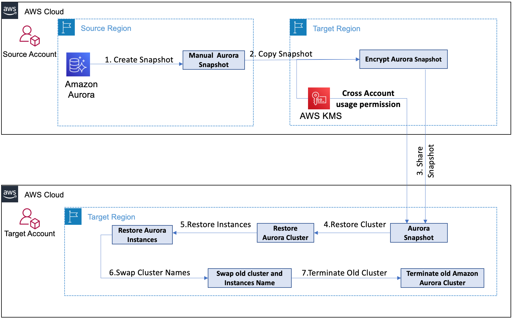
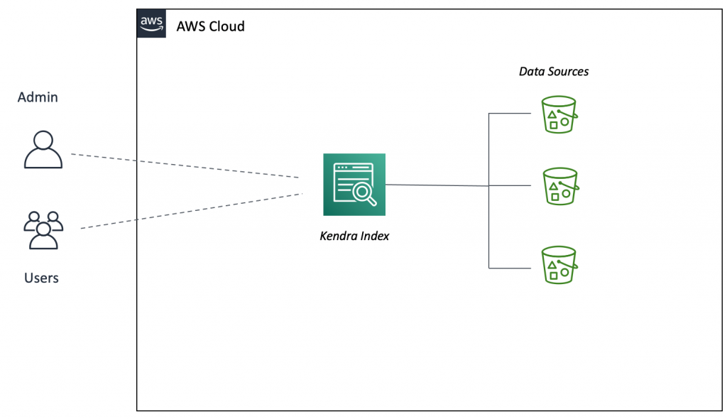
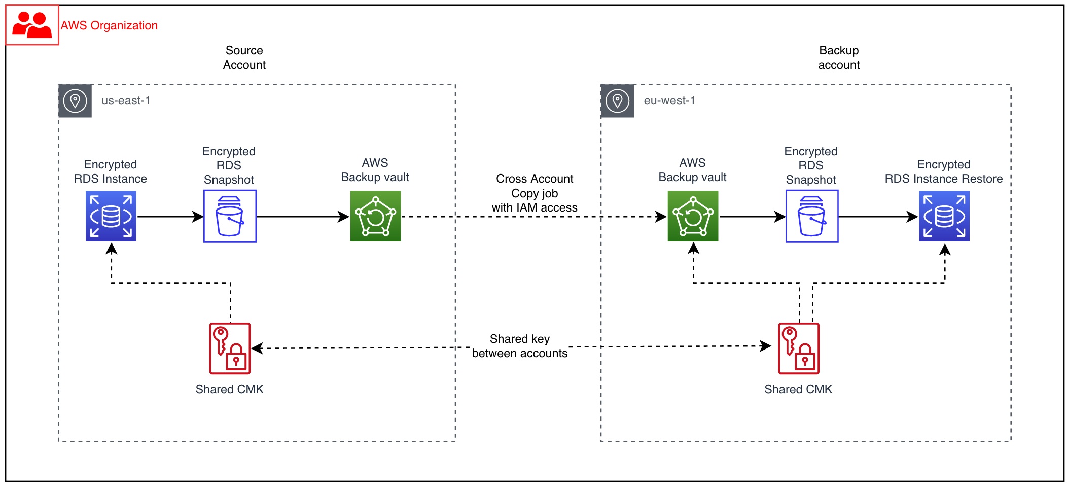
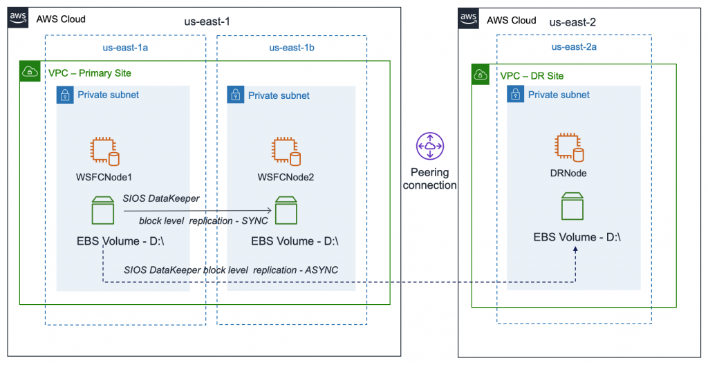
In the following architecture, we describe how you can protect your AWS workloads from outages and disasters. You can quickly set up a DR plan using Druva’s simple and intuitive user interface, and within minutes you are ready to protect your AWS infrastructure.
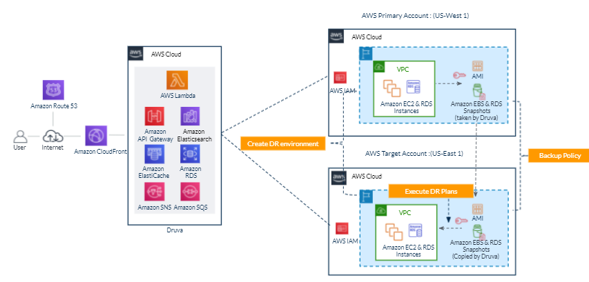
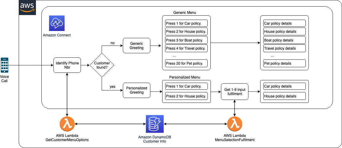
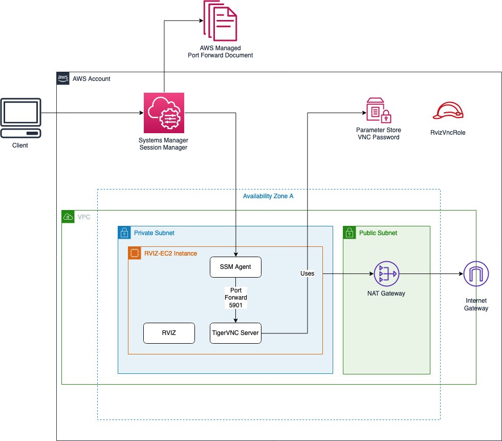
Figure 1. Druva architecture
Druva’s cloud DR is built on AWS using native services to provide a secure operating environment for comprehensive backup and DR operations. With Druva, you can:
- Seamlessly create cross-account DR sites based on source sites by cloning Amazon Virtual Private Clouds (Amazon VPCs) and their dependents.
- Set up backup policies to automatically create and copy snapshots of Amazon Elastic Compute Cloud (Amazon EC2) and Amazon Relational Database Service (Amazon RDS) instances to DR Regions based on recovery point objective (RPO) requirements.
- Set up service level objective (SLO) based DR plans with options to schedule automated tests of DR plans and ensure compliance.
- Monitor implementation of DR plans easily from the Druva console.
- Generate compliance reports for DR failover and test initiation.
Other notable features include support for automated runbook initiation, selection of target AWS instance types for DR, and simplified orchestration and testing to help protect and recover data at scale. Druva provides the flexibility to adopt evolving infrastructure across geographic locations, adhere to regulatory requirements (such as, GDPR and CCPA), and recover workloads quickly following disasters, helping meet your business-critical recovery time objectives (RTOs). This unified solution offers taking snapshots as frequently as every five minutes, improving RPOs. Because it is a software as a service (SaaS) solution, Druva helps lower costs by eliminating traditional administration and maintenance of storage hardware and software, upgrades, patches, and integrations.
We will show you how to set up Druva to protect your AWS workloads and automate DR.
Step 1: Log into the Druva platform and provide access to AWS accounts
After you sign into the Druva Cloud Platform, you will need to grant Druva third-party access to your AWS account by pressing Add New Account button, and following the steps as shown in Figure 2.
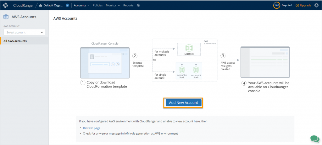
Figure 2. Add AWS account information
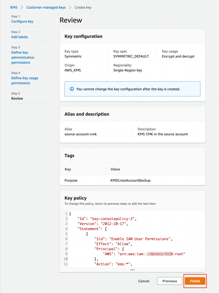
Druva uses AWS Identity and Access Management (IAM) roles to access and manage your AWS workloads. To help you with this, Druva provides an AWS CloudFormation template to create a stack or stack set that generates the following:
- IAM role
- IAM instance profile
- IAM policy
The generated Amazon Resource Name (ARN) of the IAM role is then linked to Druva so that it can run backup and DR jobs for your AWS workloads. Note that Druva follows all security protocols and best practices recommended by AWS. All access permissions to your AWS resources and Regions are controlled by IAM.
After you have logged into Druva and set up your account, you can now set up DR for your AWS workloads. The following steps will allow you to set up DR for AWS infrastructure.
Step 2: Identify the source environment
A source environment refers to a logical grouping of Amazon VPCs, subnets, security groups, and other infrastructure components required to run your application.
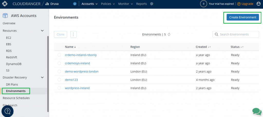
Figure 3. Create a source environment
In this step, create your source environment by selecting the appropriate AWS resources you’d like to set up for failover. Druva currently supports Amazon EC2 and Amazon RDS as sources that can be protected. With Druva’s automated DR, you can failover these resources to a secondary site with the press of a button.
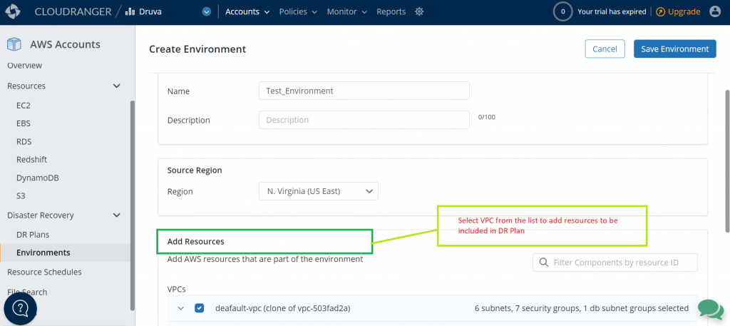
Figure 4. Add resources to a source environment
Note that creating a source environment does not create or update existing resources or configurations in your AWS account. It only saves this configuration information with Druva’s service.
Step 3: Clone the environment
The next step is to clone the source environment to a Region where you want to failover in case of a disaster. Druva supports cloning the source environment to another Region or AWS account that you have selected. Cloning essentially replicates the source infrastructure in the target Region or account, which allows the resources to be failed over quickly and seamlessly.
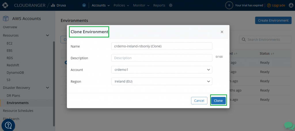
Figure 5. Clone the source environment
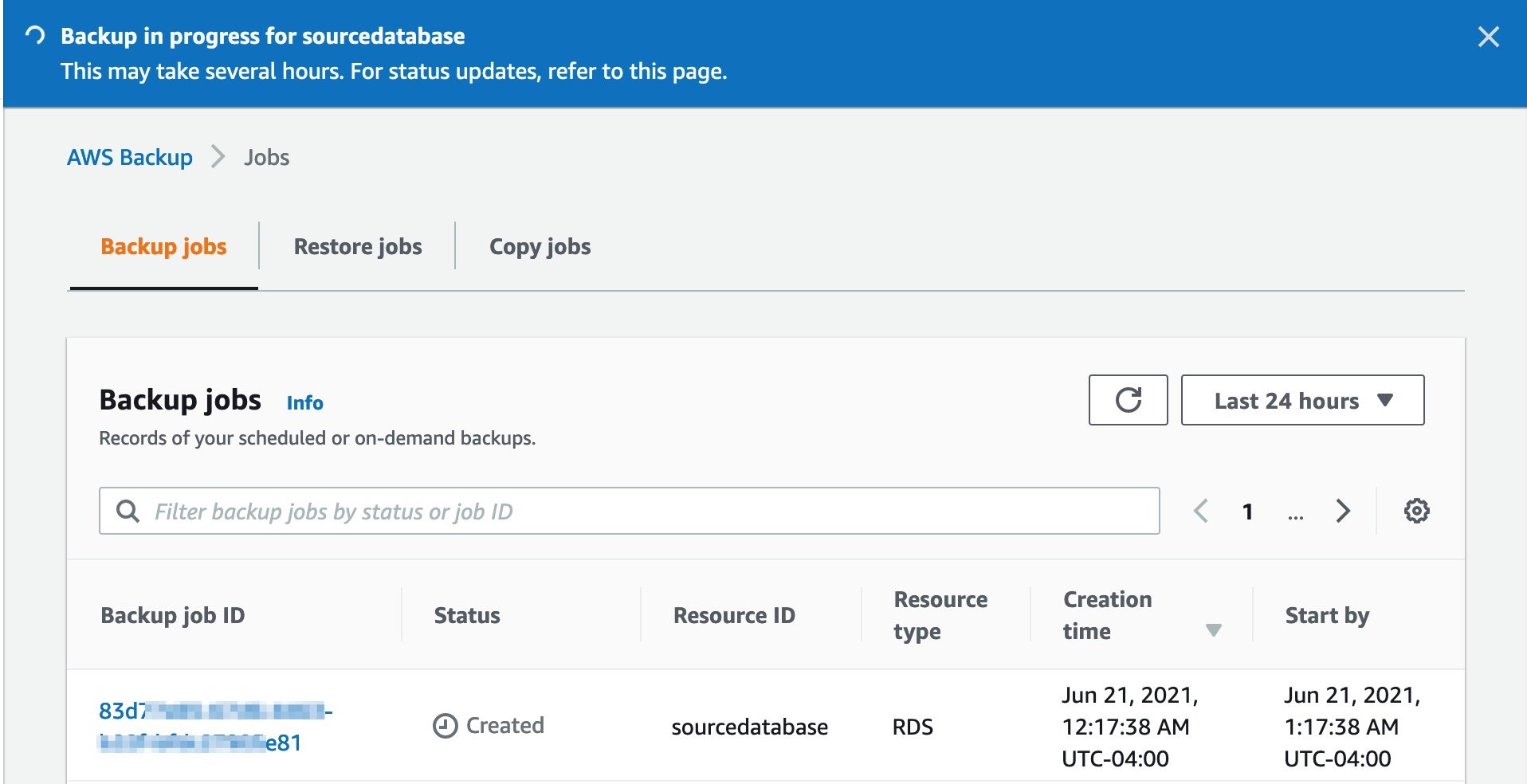
Step 4: Set up a backup policy
You can create a new backup policy or use an existing backup policy to create backups in the cloned or target Region. This enables Druva to restore instances using the backup copies.
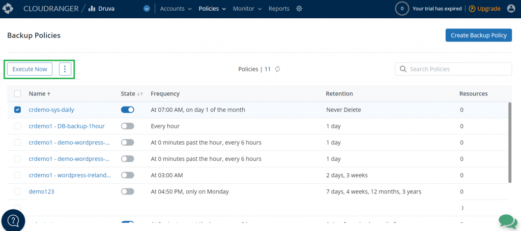
Figure 6. Create a new backup policy or use an existing backup policy
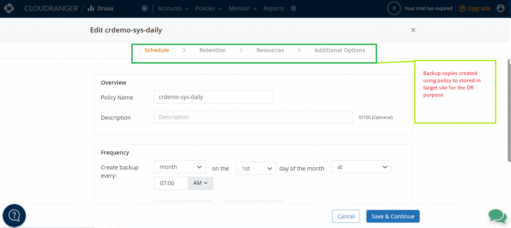
Figure 7. Customize the frequency of backup schedules
Step 5: Create the DR plan
A DR plan is a structured set of instructions designed to recover resources in the event of a failure or disaster. DR aims to get you back to the production-ready setup with minimal downtime. Follow these steps to create your DR plan.
- Create DR Plan: Press Create Disaster Recovery Plan button to open the DR plan creation page.
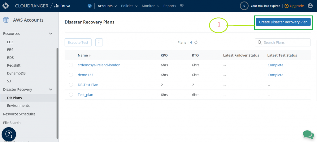
Figure 8. Create a disaster recovery plan
- Name: Enter the name of the DR plan.
Service Level Objective (SLO): Enter your RPO and RTO.
-
- Recovery Point Objective – Example: If you set your RPO as 24 hours, and your backup was scheduled daily at 8:00 PM, but a disaster occurred at 7:59 PM, you would be able to recover data that was backed up on the previous day at 8:00 PM. You would lose the data generated after the last backup (24 hours of data loss).
- Recovery Time Objective – Example: If you set your RTO as 30 hours, when a disaster occurred, you would be able to recover all critical IT services within 30 hours from the point in time the disaster occurs.
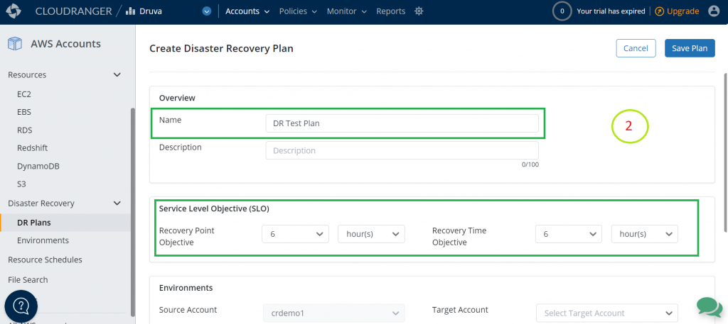
Figure 9. Add your RTO and RPO requirements
- Create your plan based off the source environment, target environment, and resources.
| Environments | |
|---|---|
| Source Account | By default, this is the Druva account in which you are currently creating the DR plan. |
| Source Environment | Select the source environment applicable within the Source Account (your Druva account in which you’re creating the DR plan). |
| Target Account | Select the same or a different target account. |
| Target Environment | Select the Target Environment, applicable within the Target Account. |
| Resources | |
|---|---|
| Create Policy | If you do not have a backup policy, then you can create one. |
| Add Resources | Add resources from the source environment that you want to restore. Make sure the verification column shows a ‘Valid Backup Policy’ status. This ensures that the backup policy is frequently creating copies as per the RPO defined previously. |
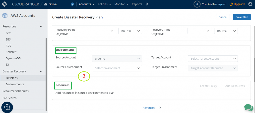
Figure 10. Create DR plan based off the source environment, target environment, and resources
- Identify target instance type, test plan instance type, and run books for this DR plan.
| Target Instance Type | Target Instance Type can be selected. If instance type is not selected then:
|
| Test Plan Instance Type | There are many options. To reduce incurring cost, the lower instance type can be selected from all available AWS instance types. |
| Run Books | Select this option if you would like to shutdown the source server after failover occurs. |
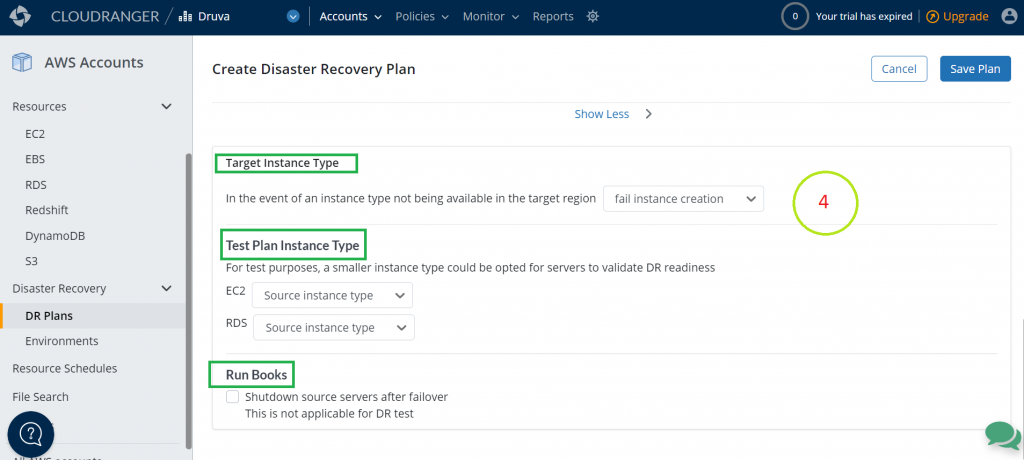
Figure 11. Identify target instance type, test plan instance type, and run books
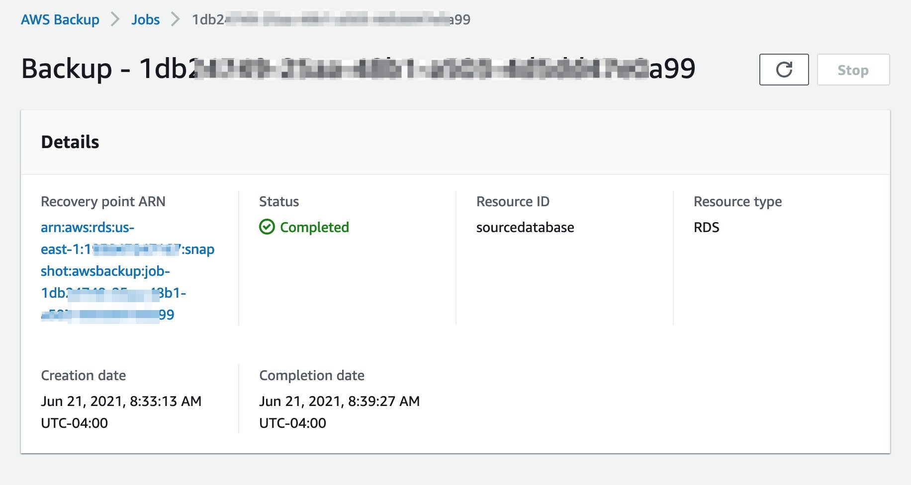
Step 6: Test the DR plan
After you have defined your DR plan, it is time to test it so that you can—when necessary—initiate a failover of resources to the target Region. You can now easily try this on the resources in the cloned environment without affecting your production environment.
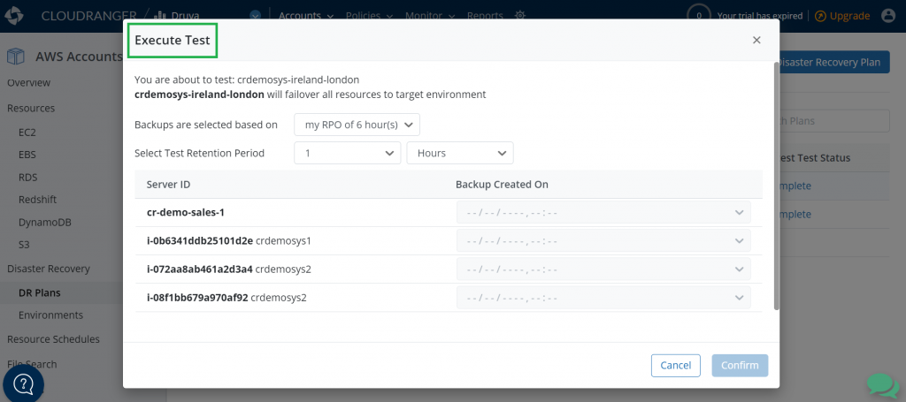
Figure 12. Test the DR plan
Testing your DR plan will help you to find answers for some of the questions like: How long did the recovery take? Did I meet my RTO and RPO objectives?
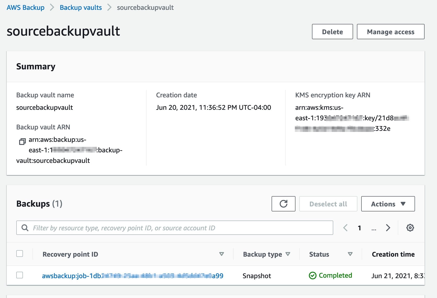
Step 7: Initiate the DR plan
After you have successfully tested the DR plan, it can easily be initiated with the click of a button to failover your resources from the source Region or account to the target Region or account.
Conclusion
With the growth of cloud-based services, businesses need to ensure that mission-critical applications that power their businesses are always available. Any loss of service has a direct impact on the bottom line, which makes business continuity planning a critical element to any organization. Druva offers a simple DR solution which will help you keep your business always available.
Druva provides unified backup and cloud DR with no need to manage hardware, software, or costs and complexity. It helps automate DR processes to ensure your teams are prepared for any potential disasters while meeting compliance and auditing requirements.
With Druva, you can easily validate your RTO and RPO with automated regular DR testing, cross-account DR for protection against attacks and accidental deletions, and ensure backups are isolated from your primary production account for DR planning. With cross-Region DR, you can duplicate the entire Amazon VPC environment across Regions to protect you against Regionwide failures. In conclusion, Druva is a complete solution built with a goal to protect your native AWS workloads from any disasters.
To learn more, visit: https://www.druva.com/use-cases/aws-cloud-backup/


 For more information, see