Tag Archives: Intermediate (200)

Analyze real-time streaming data in Amazon MSK with Amazon Athena

Post Syndicated from Scott Rigney original https://aws.amazon.com/blogs/big-data/analyze-real-time-streaming-data-in-amazon-msk-with-amazon-athena/

Recent advances in ease of use and scalability have made streaming data easier to generate and use for real-time decision-making. Coupled with market forces that have forced businesses to react more quickly to industry changes, more and more organizations today are turning to streaming data to fuel innovation and agility.

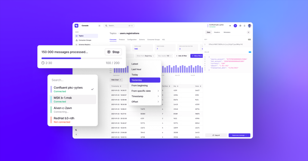
Amazon Managed Streaming for Apache Kafka (MSK) is a fully managed service that makes it easy to build and run applications that use Apache Kafka, an open-source distributed event streaming platform designed for high-performance data pipelines, streaming analytics, data integration, and mission-critical applications. With Amazon MSK, you can capture real-time data from a wide range of sources such as database change events or web application user clickstreams. Since Kafka is highly optimized for writing and reading fresh data, it’s a great fit for operational reporting. However, gaining insight from this data often requires a specialized stream processing layer to write streaming records to a storage medium like Amazon S3, where it can be accessed by analysts, data scientists, and data engineers for historical analysis and visualization using tools like Amazon QuickSight.

When you want to analyze data where it lives and without developing separate pipelines and jobs, a popular choice is Amazon Athena. With Athena, you can use your existing SQL knowledge to extract insights from a wide range of data sources without learning a new language, developing scripts to extract (and duplicate) data, or managing infrastructure. Athena supports over 25 connectors to popular data sources including Amazon DynamoDB and Amazon Redshift which give data analysts, data engineers, and data scientists the flexibility to run SQL queries on data stored in databases running on-premises or in the cloud alongside data stored in Amazon S3. With Athena, there’s no data movement and you pay only for the queries you run.

What’s new

Starting today, you can now use Athena to query streaming data in MSK and self-managed Apache Kafka. This enables you to run analytical queries on real-time data held in Kafka topics and join that data with other Kafka topics as well as other data in your Amazon S3 data lake – all without the need for separate processes to first store the data on Amazon S3.
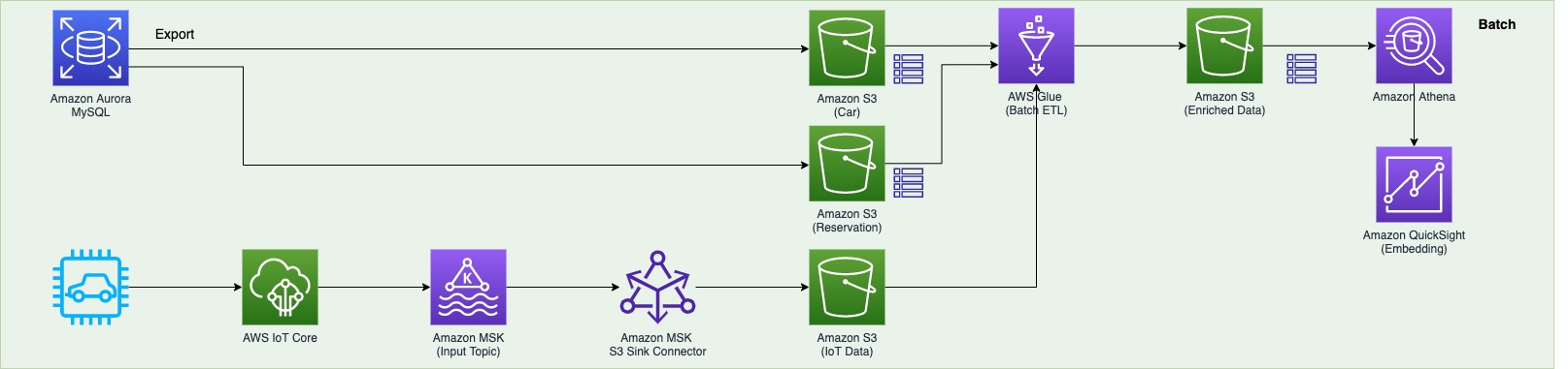
Solution overview

In this post, we show you how to get started with real-time SQL analytics using Athena and its connector for MSK. The process involves:

  1. Registering the schema of your streaming data with AWS Glue Schema Registry. Schema Registry is a feature of AWS Glue that allows you to validate and reliably evolve streaming data against JSON schemas. It can also serialize data into a compressed format, which helps you save on data transfer and storage costs.
  2. Creating a new instance of the Amazon Athena MSK Connector. Athena connectors are pre-built applications that run as serverless AWS Lambda applications, so there’s no need for standalone data export processes.
  3. Using the Athena console to run interactive SQL queries on your Kafka topics.

Get started with Athena’s connector for Amazon MSK

In this section, we’ll cover the steps necessary to set up your MSK cluster to work with Athena to run SQL queries on your Kafka topics.

Prerequisites

This post assumes you have a serverless or provisioned MSK cluster set up to receive streaming messages from a producing application. For information, see Setting up Amazon MSK and Getting started using Amazon MSK in the Amazon Managed Streaming for Apache Kafka Developer Guide.

You’ll also need to set up a VPC and a security group before you use the Athena connector for MSK. For more information, see Creating a VPC for a data source connector. Note that with MSK Serverless, VPCs and security groups are created automatically, so you can get started quickly.

Define the schema of your Kafka topics with AWS Glue Schema Registry

To run SQL queries on your Kafka topics, you’ll first need to define the schema of your topics as Athena uses this metadata for query planning. AWS Glue makes it easy to do this with its Schema Registry feature for streaming data sources.

Schema Registry allows you to centrally discover, control, and evolve streaming data schemas for use in analytics applications such as Athena. With AWS Glue Schema Registry, you can manage and enforce schemas on your data streaming applications using convenient integrations with Apache Kafka. To learn more, see AWS Glue Schema Registry and Getting started with Schema Registry.

If configured to do so, the producer of data can auto-register its schema and changes to it with AWS Glue. This is especially useful in use cases where the contents of the data is likely to change over time. However, you can also specify the schema manually and will resemble the following JSON structure.

{
  "tableName": "orders",
  "schemaName": "customer_schema",
  "topicName": "orders",
  "message": {
    "dataFormat": "json",
    "fields": [
      {
        "name": "customer_id",
        "mapping": "customer_id",
        "type": "VARCHAR"
      },
      {
        "name": "item_id",
        "mapping": "item_id",
        "type": "INTEGER"
      }
    ]
  }
}

When setting up your Schema Registry, be sure to give it an easy-to-remember name, such as customer_schema, because you’ll reference it within SQL queries as you’ll see later on. For additional information on schema set up, see Schema examples for the AWS Glue Schema Registry.

Configure the Athena connector for MSK

With your schema registered with Glue, the next step is to set up the Athena connector for MSK. We recommend using the Athena console for this step. For more background on the steps involved, see Deploying a connector and connecting to a data source.

In Athena, federated data source connectors are applications that run on AWS Lambda and handle communication between your target data source and Athena. When a query runs on a federated source, Athena calls the Lambda function and tasks it with running the parts of your query that are specific to that source. To learn more about the query execution workflow, see Using Amazon Athena Federated Query in the Amazon Athena User Guide.

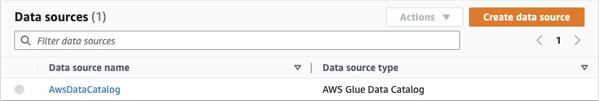
Start by accessing the Athena console and selecting Data sources on the left navigation, then choose Create data source:

Next, search for and select Amazon MSK from the available connectors and select Next.

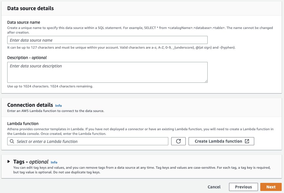
In Data source details, give your connector a name, like msk, that’s easy to remember and reference in your future SQL queries. Under Connection details section, select Create Lambda function. This will bring you to the AWS Lambda console where you’ll provide additional configuration properties.

In the Lambda application configuration screen (not shown), you’ll provide the Application settings for your connector. To do this, you’ll need a few properties from your MSK cluster and schema registered in Glue.

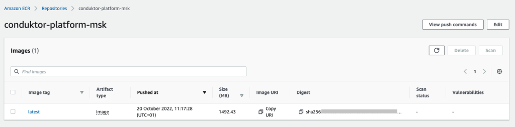
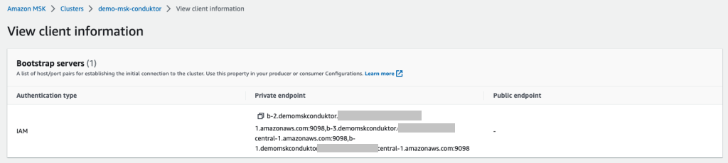
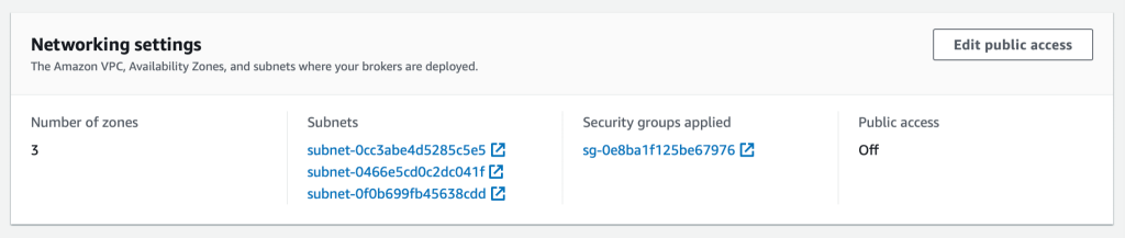
On another browser tab, use the MSK console to navigate to your MSK cluster and then select the Properties tab. Here you’ll see the VPC subnets and security group IDs from your MSK cluster which you’ll provide in the SubnetIds and SecurityGroupIds fields in the Athena connector’s Application settings form. You can find the value for KafkaEndpoint by clicking View client information.

In the AWS Glue console, navigate to your Schema Registry to find the GlueRegistryArn for the schema you wish to use with this connector.

After providing these and the other required values, click Deploy.

Return to the Athena console and enter the name of the Lambda function you just created in the Connection details box, then click Create data source.

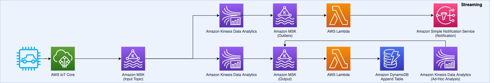
Run queries on streaming data using Athena

With your MSK data connector set up, you can now run SQL queries on the data. Let’s explore a few use cases in more detail.

Use case: interactive analysis

If you want to run queries that aggregate, group, or filter your MSK data, you can run interactive queries using Athena. These queries will run against the current state of your Kafka topics at the time the query was submitted.

Before running any queries, it may be helpful to validate the schema and data types available within your Kafka topics. To do this, run the DESCRIBE command on your Kafka topic, which appears in Athena as a table, as shown below. In this query, the orders table corresponds to the topic you specified in the Schema Registry.

DESCRIBE msk.customer_schema.orders

Now that you know the contents of your topic, you can begin to develop analytical queries. A sample query for a hypothetical Kafka topic containing e-commerce order data is shown below:

SELECT customer_id, SUM(order_total)
FROM msk.customer_schema.orders
GROUP BY customer_id

Because the orders table (and underlying Kafka topic) can contain an unbounded stream of data, the query above is likely to return a different value for SUM(order_total) with each execution of the query.

If you have data in one topic that you need to join with another topic, you can do that too:

SELECT t1.order_id, t2.item_id
FROM msk.customer_schema.orders as t1
JOIN msk.customer_schema.items as t2
ON t1.id = t2.id

Use case: ingesting streaming data to a table on Amazon S3

Federated queries run against the underlying data source which ensures interactive queries, like the ones above, are evaluated against the current state of your data. One consideration is that repeatedly running federated queries can put additional load on the underlying source. If you plan to perform multiple queries on the same source data, you can use Athena’s CREATE TABLE AS SELECT, also known as CTAS, to store the results of a SELECT query in a table on Amazon S3. You can then run queries on your newly created table without going back to the underlying source each time.

CREATE TABLE my_kafka_data
WITH (format = 'Parquet', 
      write_compression = 'SNAPPY')
AS
SELECT order_id, item_id, timestamp
FROM msk.customer_schema.orders

If you plan to do additional downstream analysis on this data, for example within dashboards on Amazon QuickSight, you can enhance the solution above by periodically adding new data to your table. To learn more, see Using CTAS and INSERT INTO for ETL and data analysis. Another benefit of this approach is that you can secure these tables with row-, column-, and table-level data governance policies powered by AWS Lake Formation to ensure only authorized users can access your table.

What else can you do?

With Athena, you can use your existing SQL knowledge to run federated queries that generate insights from a wide range of data sources without learning a new language, developing scripts to extract (and duplicate) data, or managing infrastructure. Athena provides additional integrations with other AWS services and popular analytics tools and SQL IDEs that allow you to do much more with your data. For example, you can:

  • Visualize the data in business intelligence applications like Amazon QuickSight
  • Design event-driven data processing workflows with Athena’s integration with AWS Step Functions
  • Unify multiple data sources to produce rich input features for machine learning in Amazon SageMaker

Conclusion

In this post, we learned about the newly released Athena connector for Amazon MSK. With it, you can run interactive queries on data held in Kafka topics running in MSK or self-managed Apache Kafka. This helps you bring real-time insights to dashboards or enable point-in-time analysis of streaming data to answer time-sensitive business questions. We also covered how to periodically ingest new streaming data into Amazon S3 without the need for a separate sink process. This simplifies recurring analysis of your data without incurring round-trip queries to your underlying Kafka clusters and makes it possible to secure the data with access rules powered by Lake Formation.

We encourage you to evaluate Athena and federated queries on your next analytics project. For help getting started, we recommend the following resources:


About the authors

Scott Rigney is a Senior Technical Product Manager with Amazon Web Services (AWS) and works with the Amazon Athena team based out of Arlington, Virginia. He is passionate about building analytics products that enable enterprises to make data-driven decisions.

Kiran Matty is a Principal Product Manager with Amazon Web Services (AWS) and works with the Amazon Managed Streaming for Apache Kafka (Amazon MSK) team based out of Palo Alto, California. He is passionate about building performant streaming and analytical services that help enterprises realize their critical use cases.

Prepare for consolidated controls view and consolidated control findings in AWS Security Hub

Post Syndicated from Priyanka Prakash original https://aws.amazon.com/blogs/security/prepare-for-consolidated-controls-view-and-consolidated-control-findings-in-aws-security-hub/

Currently, AWS Security Hub identifies controls and generates control findings in the context of security standards. Security Hub is aiming to release two new features in the first quarter of 2023 that will decouple controls from standards and streamline how you view and receive control findings.

The new features to be released are consolidated controls view and consolidated control findings. Consolidated controls view will provide you with a comprehensive view within the Security Hub console of your controls across security standards. This feature will also introduce a single unique identifier for each control across security standards.

Consolidated control findings will streamline your control findings. When this feature is turned on, Security Hub will produce a single finding for a security check even when a check is shared across multiple standards. This will reduce finding noise and help you focus on misconfigured resources in your AWS environment.

In this blog post, I’ll summarize the upcoming features, the benefit they bring to your organization, and how you can take advantage of them upon release.

Feature 1: Consolidated controls view

Currently, controls are identified, viewed, and managed in the context of individual security standards. In the Security Hub console, you first have to navigate to a specific standard to see a list of controls for that standard. Within the AWS Foundational Security Best Practices (FSBP) standard, Security Hub identifies controls by the impacted AWS service and a unique number (for example, IAM.1). For other standards, Security Hub includes the standard as part of the control identifier (for example, CIS 1.1 or PCI.AutoScaling.1).

After the release of consolidated controls view, you will be able to see a consolidated list of your controls from a new Controls page in the Security Hub console. Security Hub will also assign controls a consistent security control ID across standards. Following the current naming convention of the AWS FSBP standard, control IDs will include the relevant service and a unique number.

For example, the control AWS Config should be enabled is currently identified as Config.1 in the AWS FSBP standard, CIS 2.5 in the Center for Internet Security (CIS) AWS Foundations Benchmark v1.2.0, CIS 3.5 in the CIS AWS Foundations Benchmark v1.4.0, and PCI.Config.1 in the Payment Card Industry Data Security Standard (PCI DSS). After this release, this control will have a single identifier called Config.1 across standards. The single Controls page and consistent identifier will help you rapidly discover misconfigurations with minimal context-switching.

You’ll be able to enable a control for one or more enabled standards that include the control. You’ll also be able to disable a control for one or more enabled standards. As before, you can enable the standards that apply to your business case.

Changes to control finding fields and values after the release of consolidated controls view

After the release of consolidated controls view, note the following changes to control finding fields and values in the AWS Security Finding Format (ASFF).

ASFF field What changes after consolidated controls view release Example value before consolidated controls view release Example value after consolidated controls view release
Compliance.SecurityControlId A single control ID will apply across standards. ProductFields.ControlId will still provide the standards-based control ID. Not applicable (new field) EC2.2
Compliance.AssociatedStandards Will show the standards that a control is enabled for. Not applicable (new field) [{“StandardsId”: “aws-foundational-security-best-practices/v/1.0.0”}]
ProductFields.RecommendationUrl This field will no longer reference a standard. https://docs.aws.amazon.com/console/securityhub/PCI.EC2.2/remediation https://docs.aws.amazon.com/console/securityhub/EC2.2/remediation
Remediation.Recommendation.Text This field will no longer reference a standard. “For directions on how to fix this issue, please consult the AWS Security Hub PCI DSS documentation.” “For instructions on how to fix this issue, see the AWS Security Hub documentation for EC2.2.”
Remediation.Recommendation.Url This field will no longer reference a standard. https://docs.aws.amazon.com/console/securityhub/PCI.EC2.2/remediation https://docs.aws.amazon.com/console/securityhub/EC2.2/remediation

Feature 2: Consolidated control findings

Currently, multiple standards contain separate controls for the same security check. Security Hub generates a separate finding per standard for each related control that is evaluated by the same security check.

After release of the consolidated control findings feature, you’ll be able to unify control findings across standards and reduce finding noise. This, in turn, will help you more quickly investigate and remediate failed findings. When you turn on consolidated control findings, Security Hub will generate a single finding or finding update for each security check of a control, even if the check is shared across multiple standards.

For example, after you turn on the feature, you will receive a single finding for a security check of Config.1 even if you’ve enabled this control for the AWS FSBP standard, CIS AWS Foundations Benchmark v1.2.0, CIS AWS Foundations Benchmark v1.4.0, and PCI DSS. If you don’t turn on consolidated control findings, you will receive four separate findings for a security check of Config.1 if you’ve enabled this control for the AWS FSBP standard, CIS AWS Foundations Benchmark v1.2.0, CIS AWS Foundations Benchmark v1.4.0, and PCI DSS.

Changes to control finding fields and values after turning on consolidated control findings

If you turn on consolidated control findings, note the following changes to control finding fields and values in the ASFF. These changes are in addition to the changes previously described for consolidated controls view.

ASFF field What changes after consolidated controls view release Example value before consolidated controls view release Example value after consolidated controls view release
GeneratorId This field will no longer reference a standard. aws-foundational-security-best-practices/v/1.0.0/Config.1 security-control/Config.1
Title This field will no longer reference a standard. PCI.Config.1 AWS Config should be enabled {
Id This field will no longer reference a standard. arn:aws:securityhub:eu-central-1:123456789012:subscription/pci-dss/v/3.2.1/PCI.IAM.5/finding/ab6d6a26-a156-48f0-9403-115983e5a956 arn:aws:securityhub:eu-central-1:123456789012:security-control/iam.9/finding/ab6d6a26-a156-48f0-9403-115983e5a956
ProductFields.ControlId This field will be removed in favor of a single, standard-agnostic control ID. PCI.EC2.2 Removed. See Compliance.SecurityControlId instead.
ProductFields.RuleId This field will be removed in favor of a single, standard-agnostic control ID. 1.3 Removed. See Compliance.SecurityControlId instead.
Description This field will no longer reference a standard. This PCI DSS control checks whether AWS Config is enabled in the current account and region. This AWS control checks whether AWS Config is enabled in the current account and region.
Severity Security Hub will no longer use the Product field to describe the severity of a finding. “Severity”: {
“Product”: 90,
“Label”: “CRITICAL”,
“Normalized”: 90,
“Original”: “CRITICAL”
},
“Severity”: {
“Label”: “CRITICAL”,
“Normalized”: 90,
“Original”: “CRITICAL”
},
Types This field will no longer reference a standard. [“Software and Configuration Checks/Industry and Regulatory Standards/PCI-DSS”] [“Software and Configuration Checks/Industry and Regulatory Standards”]
Compliance.RelatedRequirements This field will show related requirements across associated standards. [ “PCI DSS 10.5.2”,
“PCI DSS 11.5”]
[ “PCI DSS v3.2.1/10.5.2”,
“PCI DSS v3.2.1/11.5”,
“CIS AWS Foundations Benchmark v1.2.0/2.5”]
CreatedAt Format will remain the same, but value will reset when you turn on consolidated control findings. 2022-05-05T08:18:13.138Z 2022-09-25T08:18:13.138Z
FirstObservedAt Format will remain the same, but value will reset when you turn on consolidated control findings. 2022-05-07T08:18:13.138Z 2022-09-28T08:18:13.138Z
ProductFields.RecommendationUrl This field will be replaced by Remediation.Recommendation.Url. https://docs.aws.amazon.com/console/securityhub/EC2.2/remediation Removed. See Remediation.Recommendation.Url instead.
ProductFields.StandardsArn This field will be replaced by Compliance.AssociatedStandards. arn:aws:securityhub:::standards/aws-foundational-security-best-practices/v/1.0.0 Removed. See Compliance.AssociatedStandards instead.
ProductFields.StandardsControlArn This field will be removed because Security Hub will generate one finding for a security check across standards. arn:aws:securityhub:us-east-1:123456789012:control/aws-foundational-security-best-practices/v/1.0.0/Config.1 Removed.
ProductFields.StandardsGuideArn This field will be replaced by Compliance.AssociatedStandards. arn:aws:securityhub:::ruleset/cis-aws-foundations-benchmark/v/1.2.0 Removed. See Compliance.AssociatedStandards instead.
ProductFields.StandardsGuideSubscriptionArn This field will be removed because Security Hub will generate one finding for a security check across standards. arn:aws:securityhub:us-east-2:123456789012:subscription/cis-aws-foundations-benchmark/v/1.2.0 Removed.
ProductFields.StandardsSubscriptionArn This field will be removed because Security Hub will generate one finding for a security check across standards. arn:aws:securityhub:us-east-1:123456789012:subscription/aws-foundational-security-best-practices/v/1.0.0 Removed.
ProductFields.aws/securityhub/FindingId This field will no longer reference a standard. arn:aws:securityhub:us-east-1::product/aws/securityhub/arn:aws:securityhub:us-east-1:123456789012:subscription/aws-foundational-security-best-practices/v/1.0.0/Config.1/finding/751c2173-7372-4e12-8656-a5210dfb1d67 arn:aws:securityhub:us-east-1::product/aws/securityhub/arn:aws:securityhub:us-east-1:123456789012:security-control/Config.1/finding/751c2173-7372-4e12-8656-a5210dfb1d67

New values for customer-provided finding fields after turning on consolidated control findings

When you turn on consolidated control findings, Security Hub will archive the existing findings and generate new findings. To view archived findings, you can visit the Findings page of the Security Hub console with the Record state filter set to ARCHIVED, or use the GetFindings API action. Updates you’ve made to the original finding fields in the Security Hub console or by using the BatchUpdateFindings API action will not be preserved in the new findings (if needed, you can recover this data by referring to the archived findings).

Note the following changes to customer-provided control finding fields when you turn on consolidated control findings.

Customer-provided ASFF field Description of change after turning on consolidated control findings
Confidence Will reset to empty state.
Criticality Will reset to empty state.
Note Will reset to empty state.
RelatedFindings Will reset to empty state.
Severity The default severity of the finding (matches the severity of the control).
Types Will reset to standard-agnostic value.
UserDefinedFields Will reset to empty state.
VerificationState Will reset to empty state.
Workflow New failed findings will have a default value of NEW. New passed findings will have a default value of RESOLVED.

How to turn consolidated control findings on and off

Follow these instructions to turn consolidated control findings on and off.

New accounts

If you enable Security Hub for an AWS account for the first time on or after the time when consolidated control findings is released, by default consolidated control findings will be turned on for your account. You can turn it off at any time. However, we recommend keeping it turned on to minimize finding noise.

If you use the Security Hub integration with AWS Organizations, consolidated control findings will be turned on for new member accounts if the administrator account has turned on the feature. If the administrator account has turned it off, it will be turned off for new subordinate AWS accounts (member accounts) as well.

Existing accounts

If your Security Hub account already existed before consolidated control findings is released, your account will have consolidated control findings turned off by default. You can turn it on at any time. We recommend turning it on to minimize finding noise. If you use AWS Organizations, consolidated control findings will be turned on or off for existing member accounts based on the settings of the administrator account.

To turn consolidated control findings on and off (Security Hub console)

  1. In the navigation pane, choose Settings.
  2. Choose the General tab.
  3. For Controls, turn on Consolidated control findings. Turn it off to receive multiple findings for each standard.
  4. Choose Save.

To turn consolidated control findings on and off (Security Hub API)

  • Run the UpdateSecurityHubConfiguration API action. Use the new ControlFindingGenerator attribute to change whether an account uses consolidated control findings:
    • To turn on consolidated control findings, set ControlFindingGenerator equal to SECURITY_CONTROL.
    • To turn it off, set ControlFindingGenerator equal to STANDARD_CONTROL.

To turn consolidated control findings on and off (AWS CLI)

  • In the AWS CLI, run the update-security-hub-configuration command. Use the new control-finding-generator attribute to change whether an account uses consolidated control findings:
    • To turn on consolidated control findings, set control-finding-generator equal to SECURITY_CONTROL.
    • To turn it off, set control-finding-generator equal to STANDARD_CONTROL.

API permissions for consolidated control findings

You’ll need AWS Identity and Access Management (IAM) permissions for the following new API operations in order for consolidated control findings to work as expected:

  • BatchGetSecurityControls – Returns account and Region-specific data about a batch of controls.
  • ListSecurityControlDefinitions – Returns information about controls that apply to a specified standard.
  • ListStandardsControlAssociations – Identifies whether a control is currently associated with or dissociated from each enabled standard.
  • BatchGetStandardsControlAssociations – For a batch of controls, identifies whether each control is currently associated with or dissociated from a specified standard.
  • BatchUpdateStandardsControlAssociations – Used to associate a control with enabled standards that include the control, or to dissociate a control from enabled standards. This is a batch substitute for the UpdateStandardsControl API action if an administrator doesn’t want to allow member accounts to associate or dissociate controls.
  • BatchGetControlEvaluations (private API) – Retrieves the enablement and compliance status of a control, the findings count for a control, and the overall security score for controls.

How to prepare for control finding field and value changes

If your workflows don’t rely on the specific format of any control finding fields, no action is required to prepare for the feature releases. We recommend that you immediately turn on consolidated control findings.

Consider waiting to turn on consolidated control findings if you currently rely on the Automated Security Response on AWS solution for predefined response and remediation actions. That solution does not yet support consolidated control findings. If you turn consolidated control findings on now, actions you deployed using the Automated Security Response solution will no longer work.

If you rely on the specific format of any control finding fields (for example, for custom automation), carefully review the upcoming finding field and value changes to ensure that your workflows will continue to function as intended. Note that the changes noted in the first table in this post might impact you if you rely on the specified control finding fields and values.

The changes noted in the second table and third table in this post will only impact you if you turn on consolidated control findings. For example, if you rely on ProductFields.ControlId, GeneratorId, or Title, you’ll be impacted if you turn on consolidated control findings. As another example, if you’ve created an Amazon CloudWatch Events rule that initiates an action for a specific control ID (such as invoking an AWS Lambda function if the control ID equals CIS 2.7), you’ll need to update the rule to use CloudTrail.2, the new Compliance.SecurityControlId field for that control.

If you’ve created custom insights by using the control finding fields or values that will change (see previous tables), we recommend updating those insights to use the new fields or values.

Conclusion

This post covered the control finding fields and values that will change in Security Hub after release of the consolidated controls view and consolidated control findings features. We recommend that you carefully review the changes and update your workflows to start using the new fields and values as soon as the features become available.

For more information about the upcoming changes, see the Security Hub user guide, which includes value changes for GeneratorId , control title changes, and sample control findings before and after the upcoming feature releases.

If you have feedback about this post, submit comments in the Comments section below. If you have questions about this post, start a new thread on the Security, Identity, & Compliance re:Post or contact AWS Support.

Want more AWS Security news? Follow us on Twitter.

Author

Priyanka Prakash

Priyanka is a technical writer for AWS Security Hub. She enjoys helping customers understand how to effectively monitor their environment and address security issues. Prior to joining AWS, Priyanka worked for a cloud monitoring startup. In her personal time, Priyanka enjoys cooking and hiking.

Create, Train and Deploy Multi Layer Perceptron (MLP) models using Amazon Redshift ML

Post Syndicated from Anuradha Karlekar original https://aws.amazon.com/blogs/big-data/create-train-and-deploy-multi-layer-perceptron-mlp-models-using-amazon-redshift-ml/

Amazon Redshift is a fully managed and petabyte-scale cloud data warehouse which is being used by tens of thousands of customers to process exabytes of data every day to power their analytics workloads. Amazon Redshift comes with a feature called Amazon Redshift ML which puts the power of machine learning in the hands of every data warehouse user, without requiring the users to learn any new programming language, ML concepts or ML tools. Redshift ML abstracts all the intricacies that are involved in the traditional ML approach around data warehouse which traditionally involved repetitive, manual steps to move data back and forth between the data warehouse and ML tools for running long, complex, iterative ML workflow.

Redshift ML uses Amazon SageMaker Autopilot and Amazon SageMaker Neo in the background to make it easy for SQL users such as data analysts, data scientists, BI experts and database developers to create, train, and deploy machine learning (ML) models using familiar SQL commands and then use these models to make predictions on new data for use cases such as customer churn prediction, basket analysis for sales prediction, manufacturing unit lifetime value prediction, and product recommendations. Redshift ML makes the model available as SQL function within the Amazon Redshift data warehouse so you can easily use it in queries and reports.

Amazon Redshift ML supports supervised learning, including regression, binary classification, multi-class classification, and unsupervised learning using K-Means. You can optionally specify XGBoost, MLP, and linear learner model types, which are supervised learning algorithms used for solving either classification or regression problems, and provide a significant increase in speed over traditional hyperparameter optimization techniques. Amazon Redshift ML also supports bring-your-own-model to either import existing SageMaker models that are built using algorithms supported by SageMaker Autopilot, which can be used for local inference; or for the unsupported algorithms, one can alternatively invoke remote SageMaker endpoints for remote inference.

In this blog post, we show you how to use Redshift ML to solve binary classification problem using the Multi Layer Perceptron (MLP) algorithm, which explores different training objectives and chooses the best solution from the validation set.

A multilayer perceptron (MLP) is a deep learning method which deals with training multi-layer artificial neural networks, also called Deep Neural Networks. It is a feedforward artificial neural network that generates a set of outputs from a set of inputs. An MLP is characterized by several layers of input nodes connected as a directed graph between the input and output layers. MLP uses backpropagation for training the network. MLP is widely used for solving problems that require supervised learning as well as research into computational neuroscience and parallel distributed processing. It is also used for speech recognition, image recognition and machine translation.

As far as MLP usage with Redshift ML (powered by Amazon SageMaker Autopilot) is concerned, it supports tabular data as of now.

Solution Overview

To use the MLP algorithm, you need to provide inputs or columns representing dimensional values and also the label or target, which is the value you’re trying to predict.

With Redshift ML, you can use MLP on tabular data for regression, binary classification or multiclass classification problems. What is more unique about MLP is, is that the output function of MLP can be a linear or a continuous function as well. It need not be a straight line like the general regression model provides.

In this solution, we use binary classification to detect frauds based upon the credit cards transaction data. The difference between classification models and MLP is that logistic regression uses a logistic function, while perceptrons use a step function. Using the multilayer perceptron model, machines can learn weight coefficients that help them classify inputs. This linear binary classifier is highly effective in arranging and categorizing input data into different classes, allowing probability-based predictions and classifying items into multiple categories. Multilayer Perceptrons have the advantage of learning non-linear models and the ability to train models in real-time.

For this solution, we first ingest the data into Amazon Redshift, we then distribute it for model training and validation, then use Amazon Redshift ML specific queries for model creation and thereby create and utilize the generated SQL function for being able to finally predict the fraudulent transactions.

Prerequisites

To get started, we need an Amazon Redshift cluster or an Amazon Redshift Serverless endpoint and an AWS Identity and Access Management (IAM) role attached that provides access to SageMaker and permissions to an Amazon Simple Storage Service (Amazon S3) bucket.

For an introduction to Redshift ML and instructions on setting it up, see Create, train, and deploy machine learning models in Amazon Redshift using SQL with Amazon Redshift ML.

To create a simple cluster with a default IAM role, see Use the default IAM role in Amazon Redshift to simplify accessing other AWS services.

Data Set Used

In this post, we use the Credit Card Fraud detection data to create, train and deploy MLP model which can be used further to identify fraudulent transactions from the newly captured transaction records.

The dataset contains transactions made by credit cards in September 2013 by European cardholders.
This dataset presents transactions that occurred in two days, where we have 492 frauds out of 284,807 transactions. The dataset is highly unbalanced, the positive class (frauds) account for 0.172% of all transactions.

It contains only numerical input variables which are the result of a Principal Component Analysis transformation. Due to confidentiality issues, the original features and more background information about the data is not provided. Features V1, V2, … V28 are the principal components obtained with PCA, the only features which have not been transformed with PCA are ‘Time’ and ‘Amount’. Feature ‘Time’ contains the seconds elapsed between each transaction and the first transaction in the dataset. The feature ‘Amount’ is the transaction Amount. Feature ‘Class’ is the response variable and it takes value 1 in case of fraud and 0 otherwise.

Here are sample records:

Prepare the data

Load the credit card dataset into Amazon Redshift using the following SQL. You can use the Amazon Redshift query editor v2 or your preferred SQL tool to run these commands.

Alternately we have provided a notebook you may use to execute all the sql commands that can be downloaded here. You will find instructions in this blog on how to import and use notebooks.

To create the table, use the following command:

CREATE TABLE creditcardsfrauds (
    txtime integer,
    v1 float8,
    v2 float8,
    v3 float8,
    v4 float8,
    v5 float8,
    v6 float8,
    v7 float8,
    v8 float8,
    v9 float8,
    v10 float8,
    v11 float8,
    v12 float8,
    v13 float8,
    v14 float8,
    v15 float8,
    v16 float8,
    v17 float8,
    v18 float8,
    v19 float8,
    v20 float8,
    v21 float8,
    v22 float8,
    v23 float8,
    v24 float8,
    v25 float8,
    v26 float8,
    v27 float8,
    v28 float8,
    amount float8,
    class integer
);

Load the data

To load data into Amazon Redshift, use the following COPY command:

COPY creditcardsfrauds
FROM 's3://redshift-ml-blog-mlp/creditcard.csv' 
IAM_ROLE default
CSV QUOTE as '\"' delimiter ',' IGNOREHEADER 1 maxerror 100
REGION 'us-east-1';

Before creating the model, we want to divide our data into two sets by splitting 80% of the dataset for training and 20% for validation, which is a common practice in ML. The training data is input to the ML model to identify the best possible algorithm for the model. After the model is created, we use the validation data to validate the model accuracy.

So, in ‘creditcardsfrauds’ table, we check the distribution of data based upon ‘txtime’ value and identify the cutoff for around 80% of the data to train the model.

With this, the highest txtime value comes to 120954 (based upon the distribution of txtime’s min, max, ranking by window function and ceil(count(*)*0.80) values)), based upon which we consider the transaction records having ‘txtime’ field value less than 120954 for creating training data. We then validate the accuracy of that model by seeing if it correctly identifies the fraudulent transactions by predicting its ‘class’ attribute on the remaining 20% of the data.

This distribution for 80% cutoff need not always be based upon ordered time. It can be picked up randomly as well, based upon the use case under consideration.

Create a model in Redshift ML

To create the model, use the following command:

 CREATE model creditcardsfrauds_mlp
FROM (select * from creditcardsfrauds where txtime < 120954)
TARGET class 
FUNCTION creditcardsfrauds_mlp_fn
IAM_ROLE default
MODEL_TYPE MLP
SETTINGS (
      S3_BUCKET '<<your-amazon-s3-bucket-name>>’,
      MAX_RUNTIME 9600
);

Here, in the settings section of the command, you need to set up an S3_BUCKET which is used to export the data that is sent to SageMaker and store model artifacts.

S3_BUCKET setting is a required parameter of the command, whereas MAX_RUNTIME is an optional one which specifies the maximum amount of time to train. The default value of this parameter is 90 minutes (5400 seconds), however you can override it by explicitly specifying it in the command, just like we have done it here by setting it to run for 9600 seconds.

The preceding statement initiates an Amazon SageMaker Autopilot process in the background to automatically build, train, and tune the best ML model for the input data. It then uses Amazon SageMaker Neo to deploy that model locally in the Amazon Redshift cluster or Amazon Redshift Serverless as a user-defined function (UDF).

You can use the SHOW MODEL command in Amazon Redshift to track the progress of your model creation, which should be in the READY state within the max_runtime parameter you defined while creating the model.

To check the status of the model, use the following command:

show model creditcardsfrauds_mlp;

We notice from the preceding table that the F1-score for the training data is 0.908, which shows very good performance accuracy.

To elaborate, F1-score is the harmonic mean of precision and recall. It combines precision and recall into a single number using the following formula:

Where, Precision means: Of all positive predictions, how many are really positive?

And Recall means: Of all real positive cases, how many are predicted positive?

F1 scores can range from 0 to 1, with 1 representing a model that perfectly classifies each observation into the correct class and 0 representing a model that is unable to classify any observation into the correct class. So higher F1 scores are better.

The following is the detailed tabular outcome for the preceding command after model training was done.

Model Name creditcardsfrauds_mlp
Schema Name public
Owner redshiftml
Creation Time Sun, 25.09.2022 16:07:18
Model State READY
validation:binary_f_beta 0.908864
Estimated Cost 112.296925
TRAINING DATA: .
Query SELECT * FROM CREDITCARDSFRAUDS WHERE TXTIME < 120954
Target Column CLASS
PARAMETERS: .
Model Type mlp
Problem Type BinaryClassification
Objective F1
AutoML Job Name redshiftml-20221118035728881011
Function Name creditcardsfrauds_mlp_fn
. creditcardsfrauds_mlp_fn_prob
Function Parameters txtime v1 v2 v3 v4 v5 v6 v7 v8 v9 v10 v11 v12 v13 v14 v15 v16 v17 v18 v19 v20 v21 v22 v23 v24 v25 v26 v27 v28 amount
Function Parameter Types int4 float8 float8 float8 float8 float8 float8 float8 float8 float8 float8 float8 float8 float8 float8 float8 float8 float8 float8 float8 float8 float8 float8 float8 float8 float8 float8 float8 float8 float8
IAM Role default
S3 Bucket redshift-ml-blog-mlp
Max Runtime 54000

Redshift ML now supports Prediction Probabilities for binary classification models. For classification problem in machine learning, for a given record, each label can be associated with a probability that indicates how likely this record really belongs to the label. With option to have probabilities along with the label, customers could use the classification results when confidence based on chosen label is higher than a certain threshold value returned by the model

Prediction probabilities are calculated by default for binary classification models and an additional function is created while creating model without impacting performance of the ML model.

In above snippet, you will notice that predication probabilities enhancements have added another function as a suffix (_prob) to model function with a name ‘creditcardsfrauds_mlp_fn_prob’ which could be used to get prediction probabilities.

Additionally, you can check the model explainability to understand which inputs contributed effectively to derive the prediction.

Model explainability helps to understand the cause of prediction by answering questions such as:

  • Why did the model predict a negative outcome such as blocking of credit card when someone travels to a different country and withdraws a lot of money in different currency?
  • How does the model make predictions? Lots of data for credit cards can be put in a tabular format and as per MLP process where a fully connected neural network of several layers is involved, we can tell which input feature actually contributed to the model output and its magnitude.
  • Why did the model make an incorrect prediction? E.g. Why is the card blocked even though the transaction is legitimate?
  • Which features have the largest influence on the behavior of the model? Is it just based upon the location where the credit card is swiped, or even the time of the day and unusual credit consumption that is influencing the prediction?

Run the following SQL command to retrieve the values from the explainability report:

SELECT json_table.report.explanations.kernel_shap.label0.global_shap_values 
FROM (select explain_model('creditcardsfrauds_mlp') as report) as json_table;

In the preceding screenshot, we have only selected the column that projects shapley values from the response returned by the explain_model function. If you notice the response of the query, the values in every json object show the contribution of different features in terms of influencing the prediction. E.g. from the preceding snippet, v14 feature is influencing the prediction the most and txtime feature does not really play any significant role in predicting ‘class’.

Model validation

Now let’s run the prediction query and validate the accuracy of the model on the validation dataset:

FROM (
  SELECT 
      CASE WHEN class =  
      creditcardsfrauds_mlp_fn(txtime,v1,v2,v3,v4,v5,v6,v7,v8,v9,v10,v11,v12,v13,v14,v15,v16,v17,v18,v19,v20,v21,v22,v23,v24,v25,v26,v27,v28,amount) 
      THEN 'PredictedMatchesActual' 
      else 'NoMatch' 
      END as actualvspredicted
    FROM creditcardsfrauds 
    WHERE txtime >= 120954
) 
group by actualvspredicted

We can observe here that Redshift ML is able to identify 99.88 percent of the transactions correctly as fraudulent or non-fraudulent.

Now you can continue to use this SQL function creditcardsfrauds_mlp_fn for local inference in any part of the SQL query while analyzing, visualizing or reporting the newly arriving as well as existing data!

--CREATE A STAGING TABLE TO HOLD NEWLY ARRIVING DATA FROM THE SOURCE WHICH WILL NOT CONAIN THE CLASS COLUMN - AS IT IS TO BE PREDICTED
DROP TABLE creditcardsfrauds_staging;
CREATE TABLE creditcardsfrauds_staging as (select * from creditcardsfrauds limit 0);
Alter table creditcardsfrauds_staging drop column class;

--LETS CONSIDER ONLY ONE RECORD HERE WHICH HAS NEWLY ARRIVED
insert into creditcardsfrauds_staging values(174965,-39999.11383160738512,0.58586417180689,-5.39973021073242,1.81709247345531,-0.840618465991056,-2.94354779071974,-2.20800192003372,1.05873267723056,-1.63233334974982,-5000.24598383776964,11.93351953683592,-53046479695456,-1.12745457501155,-666666.41662797597451,0.141237234328704,-2.54949823633632,-4.61471706851594,-10.47813794126038,-0.0354803664667244,0.306270740368093,0.583275998701341,-0.269208637986581,-0.456107772584008,-0.183659129549716,-0.328167759255761,0.606115810329683,0.884875539542905,-0.253700318894381,-2450000000);

--USE THE FUNCTION TO PREDICT THE VALUE OF CLASS
SELECT txtime, creditcardsfrauds_mlp_fn(txtime,v1,v2,v3,v4,v5,v6,v7,v8,v9,v10,v11,v12,v13,v14,v15,v16,v17,v18,v19,v20,v21,v22,v23,v24,v25,v26,v27,v28,amount)
FROM creditcardsfrauds_staging;

Here the output 1 means that the newly captured transaction is fraudulent as per the inference.

Additionally, you can change the above query to include prediction probabilities of label output for the above scenario and decide if you still like to use the prediction by the model.

--USE THE FUNCTION TO PREDICT THE VALUE OF CLASS ALONG WITH THE PROBABILITY
Select txtime, predictedActive.labels[0], predictedActive.probabilities[0] 
from (
SELECT txtime, creditcardsfrauds_mlp_fn_prob(txtime,v1,v2,v3,v4,v5,v6,v7,v8,v9,v10,v11,v12,v13,v14,v15,v16,v17,v18,v19,v20,v21,v22,v23,v24,v25,v26,v27,v28,amount)as predictedACtive
FROM creditcardsfrauds_staging ) temp

The above screenshot shows that this transaction has 100% likelihood of being fraudulent.

Clean up

To avoid incurring future charges, you can stop the Redshift cluster when not being used. You can even terminate the Redshift cluster altogether if you have run the exercise in this blog post just for experimental purpose. If you are instead using serverless version of Redshift, it will not cost you anything, until it is used. However, like mentioned before, you will have to stop or terminate the cluster if you are using a provisioned version of Redshift.

Conclusion

Redshift ML makes it easy for users of all levels to create, train, and tune models using SQL interface. In this post, we walked you through how to use the MLP algorithm to create binary classification model. You can then use those models to make predictions using simple SQL commands and gain valuable insights.

To learn more about RedShift ML, visit Amazon Redshift ML.


About the authors

Anuradha Karlekar is a Solutions Architect at AWS working majorly for Partners and Startups. She has over 15 years of IT experience extensively in full stack development, deployment, building data ETL pipelines and visualizations. She is passionate about data analytics and text search. Outside work – She is a travel enthusiast!

Phil Bates is a Senior Analytics Specialist Solutions Architect at AWS with over 25 years of data warehouse experience.

Abhishek Pan is a Solutions Architect-Analytics working at AWS India. He engages with customers to define data driven strategy, provide deep dive sessions on analytics use cases & design  scalable and performant Analytical applications. He has over 11 years of experience and is passionate about Databases, Analytics and solving customer problems with help of cloud solutions. An avid traveller and tries to capture world through my lenses

Debu Panda is a Senior Manager, Product Management at AWS, is an industry leader in analytics, application platform, and database technologies, and has more than 25 years of experience in the IT world. Debu has published numerous articles on analytics, enterprise Java, and databases and has presented at multiple conferences such as re:Invent, Oracle Open World, and Java One. He is lead author of the EJB 3 in Action (Manning Publications 2007, 2014) and Middleware Management (Packt).

Scaling AWS Outposts rack deployments with ACE racks

Post Syndicated from Sheila Busser original https://aws.amazon.com/blogs/compute/scaling-aws-outposts-rack-deployments-with-ace-racks/

This blog post is written by Eric Vasquez, Specialist Hybrid Edge Solutions Architect, and Paul Scherer, Senior Network Service Tech.

Overview

AWS Outposts brings managed, monitored AWS infrastructure, compute, and storage to your on-premises environment. It provides the same AWS APIs, and console experience you would get within the AWS Region to which the Outpost is homed to. You may already have an Outposts rack. An Outpost can consist of one or more racks creating a pool of consumable resources as a single logical Outpost. In this post, we will introduce you to an Aggregation, Core, Edge (ACE) rack.

Depending on your familiarity with the Outpost family, you might have already heard about an ACE rack. An ACE rack serves as an aggregation point for multi-rack Outpost deployments. ACE racks reduce the physical networking port requirements as well as the logical interfaces needed, while allowing for connectivity between multiple racks in your logical Outpost. ACE racks are recommended for customers with planned deployments beyond three racks excluding the ACE rack itself.

We recommend that all customers leverage an ACE rack if planning expansions beyond three racks in the long-term, even if the initial deployment is a single rack. An ACE rack contains four routers, and these routers can connect to either two or four customer upstream devices. For the best redundancy, reliability, and resiliency, we recommend deploying an ACE rack to four upstream customer devices.

ACE racks support 10G, 40G, and 100G connections to a customer network. However, 100G connections between each ACE router to a customer device are recommended.

Outpost architecture aceOutpost extension from region and ACE rack deployment in a 15 rack Outpost configuration

Each Outposts rack comes standard with redundant Outpost networking devices, power supplies, and two top-of-rack patch panels which serve as demarcation points between the Outpost rack and your customer networking device (CND). For the remainder of this post, we’ll refer to the Outpost Networking Devices as OND and customer switches/routers as CND. The Outpost rack ONDs form Border Gateway Protocol (BGP) neighbor relationships with either your CND or the ACE rack using point-to-point (P2P) Virtual LAN (VLAN) interfaces.

For Outposts installation without an ACE rack, each Outposts OND connects to your LAN using single-mode or multi-mode fiber with LC connectors supporting 1G, 10G, 40G, or 100G connectivity. We provide flexibility for the CNDs and allow either Layer 2 or Layer 3 devices, including firewalls. Each OND uses a single LACP port channel that carries 2 VLAN point-to-points virtual interfaced (VIF)to establish 2 BGP relationships over the port channel to your upstream CND and aggregate total bandwidth. This results in each Outpost rack requiring a minimum of two physical uplinks, but as a general best practice we recommend two-per-device for a total of four uplinks, along with two LACP port channels and 4 VLAN to establish point-to-points (P2P) BGP peering’s. Note that the IP’s used in the following diagram are just examples.

Outpost Service link and Local Gateway VLANOutpost Service link and Local Gateway VLAN

As we continue to expand rack deployments, so will the number of physical uplinks and VLAN interfaces required for the added OND to a CND. When we introduce the ACE rack, the OND is no longer attached to your CND. Instead, it goes directly to ACE devices, which provide at least one uplink to your network switch/router. In this topology, AWS owns the VLAN interface allocation and configuration between compute rack OND and the ACE routers.

Let’s cover the potential downsides to a multi-rack installation without an ACE rack. In this case, we have a three-rack Outpost deployment, with one uplink (two per rack) from each rack OND to the CND. This would require you to provide: six physical ports on your devices, six fiber cables,12 VLAN VIFs, 12 P2P subnets potentially exhausting 24 ips, and six port channels.

In comparison to a three-rack install that sits behind an ACE rack, you provide fewer physical network ports on your devices, fewer fiber cabling uplinks, fewer VLAN VIFs, fewer port channels, and fewer P2P’s. Each ACE router will have its own LACP port channel with 2x VLAN VIFs in each channel (the same as an Outposts Networking Devices (OND) <> Customer connection). The following table highlights the advantages in using an ACE rack when running a multi-rack Outpost, which becomes more desirable as you continue to scale.

2-Rack Outpost

Installation

3-Rack Outpost

Installation

4-Rack Outpost

Installation

Requirement

Without ACE With ACE Without ACE With ACE Without ACE With ACE

Physical Ports

4

4

6

4

8

4

Fiber Cables

4

4 6 4 8

4

LACP Port Channels

4

4 6 4

8

4

VLAN VIFs

8

8 12 8 16

8

P2P Subnets 8 8 12 8 16

8

ACE VS Non-ACE Rack Components Comparison

Furthermore, you should consider the additional weight, and power requirements that an ACE rack introduces when planning for multi-rack deployments. In addition to initial kVA requirements for the Outpost racks you must account for the resources required for an ACE rack. An ACE rack consumes up to 10kVA of power and weighs up to 705 lbs. Carefully planning additional capacity for these resources with your AWS account team will be critical for a successful deployment.

Similar to an Outpost rack, an ACE rack deployment is monitored by AWS. The rack provides telemetry data transmitted over a set of VPN tunnels back to the anchor points in the Region to which the Outpost is homed. This allows AWS to monitor the rack for hardware failures, performance degradation, and other alarm conditions including Links, Interfaces going down, and BGP drops.

As part of the Outpost ordering process, AWS will work closely with you to determine the location for install, power availability on-site, and the network configuration of both the Outposts rack and ACE rack. This includes BGP configuration, and the Customer Owned IP Address (CoIP), which is the pool of IP addresses for route advertisements back to your CND. The COIP pool allows resources inside your Outpost rack to communicate with on-premises resources and vice-versa. Another connectivity option would be the Direct VPC Routing (DVR) where we advertise VPC subnets associated with your LGW to your on-premises networks. Outposts uses a networking connectivity back to the Region for management purposes called the service link (SL). The SL is an encrypted set of VPN connections used whenever the Outpost communicates with your chosen home Region.

Conclusion

This post addresses the most common questions surrounding ACE racks, how an ACE rack can be deployed, and why an ACE rack would be leveraged for a multi-Outpost rack deployment. In this post, we demonstrated how an ACE rack serves as a consolidation point in your on-premises environment, making multi-rack deployments scalable, while reducing complexity and physical port allocation for connectivity between an Outpost and your LAN. In addition, we described how you can get this process started. If you want to learn more about Outposts fundamentals and how you can build your applications with AWS services using Outposts for hybrid cloud deployments you can learn more check out the Outposts user guide.

How dynamic data masking support in Amazon Redshift helps achieve data privacy and compliance

Post Syndicated from Rohit Vashishtha original https://aws.amazon.com/blogs/big-data/how-dynamic-data-masking-support-in-amazon-redshift-helps-achieve-data-privacy-and-compliance/

Amazon Redshift is a fully managed, petabyte-scale, massively parallel data warehouse that offers simple operations and high performance. It makes it fast, simple, and cost-effective to analyze all your data using standard SQL and your existing business intelligence (BI) tools. Today, Amazon Redshift is the most widely used cloud data warehouse.

Dynamic data masking (DDM) support (preview) in Amazon Redshift enables you to simplify the process of protecting sensitive data in your Amazon Redshift data warehouse. You can now use DDM to protect data based on your job role or permission rights and level of data sensitivity through a SQL interface. DDM support (preview) in Amazon Redshift enables you to hide, obfuscate, or pseudonymize column values within the tables in your data warehouse without incurring additional storage costs. It is configurable to allow you to define consistent, format-preserving, and irreversible masked data values.

DDM support (preview) in Amazon Redshift provides a native feature to support your need to mask data for regulatory or compliance requirements, or to increase internal privacy standards. Compared to static data masking where underlying data at rest gets permanently replaced or redacted, DDM support (preview) in Amazon Redshift enables you to temporarily manipulate the display of sensitive data in transit at query time based on user privilege, leaving the original data at rest intact. You control access to data through masking policies that apply custom obfuscation rules to a given user or role. That way, you can respond to changing privacy requirements without altering the underlying data or editing SQL queries.

With DDM support (preview) in Amazon Redshift, you can do the following:

  • Define masking policies that apply custom obfuscation policies (for example, masking policies to handle credit card, PII entries, HIPAA or GDPR needs, and more)
  • Transform the data at query time to apply masking policies
  • Attach masking policies to roles or users
  • Attach multiple masking policies with varying levels of obfuscation to the same column in a table and assign them to different roles with priorities to avoid conflicts
  • Implement cell-level masking by using conditional columns when creating your masking policy
  • Use masking policies to partially or completely redact data, or hash it by using user-defined functions (UDFs)

Here’s what our customers have to say on DDM support(private beta) in Amazon Redshift:

“Baffle delivers data-centric protection for enterprises via a data security platform that is transparent to applications and unique to data security. Our mission is to seamlessly weave data security into every data pipeline. Previously, to apply data masking to an Amazon Redshift data source, we had to stage the data in an Amazon S3 bucket. Now, by utilizing the Amazon Redshift Dynamic Data Masking capability, our customers can protect sensitive data throughout the analytics pipeline, from secure ingestion to responsible consumption reducing the risk of breaches.”

-Ameesh Divatia, CEO & co-founder of Baffle

“EnergyAustralia is a leading Australian energy retailer and generator, with a mission to lead the clean energy transition for customers in a way that is reliable, affordable and sustainable for all. We enable all corners of our business with Data & Analytics capabilities that are used to optimize business processes and enhance our customers’ experience. Keeping our customers’ data safe is a top priority across our teams. In the past, this involved multiple layers of custom built security policies that could make it cumbersome for analysts to find the data they require. The new AWS dynamic data masking feature will significantly simplify our security processes so we continue to keep customer data safe, while also reducing the administrative overhead.”

-William Robson, Data Solutions Design Lead, EnergyAustralia

Use case

For our use case, a retail company wants to control how they show credit card numbers to users based on their privilege. They also don’t want to duplicate the data for this purpose. They have the following requirements:

  • Users from Customer Service should be able to view the first six digits and the last four digits of the credit card for customer verification
  • Users from Fraud Prevention should be able to view the raw credit card number only if it’s flagged as fraud
  • Users from Auditing should be able to view the raw credit card number
  • All other users should not be able to view the credit card number

Solution overview

The solution encompasses creating masking policies with varying masking rules and attaching one or more to the same role and table with an assigned priority to remove potential conflicts. These policies may pseudonymize results or selectively nullify results to comply with retailers’ security requirements. We refer to multiple masking policies being attached to a table as a multi-modal masking policy. A multi-modal masking policy consists of three parts:

  • A data masking policy that defines the data obfuscation rules
  • Roles with different access levels depending on the business case
  • The ability to attach multiple masking policies on a user or role and table combination with priority for conflict resolution

The following diagram illustrates how DDM support (preview) in Amazon Redshift policies works with roles and users for our retail use case.

For a user with multiple roles, the masking policy with the highest attachment priority is used. For example, in the following example, Ken is part of the Public and FrdPrvnt role. Because the FrdPrvnt role has a higher attachment priority, card_number_conditional_mask will be applied.

Prerequisites

To implement this solution, you need to complete the following prerequisites:

  1. Have an AWS account.
  2. Have an Amazon Redshift cluster provisioned with DDM support (preview) or a serverless workgroup with DDM support (preview).
    1. Navigate to the provisioned or serverless Amazon Redshift console and choose Create preview cluster.
    2. In the create cluster wizard, choose the preview track.
  3. Have Superuser privilege, or the sys:secadmin role on the Amazon Redshift data warehouse created in step 2.

Preparing the data

To set up our use case, complete the following steps:

  1. On the Amazon Redshift console, choose Query editor v2 in Explorer.
    If you’re familiar with SQL Notebooks, you can download the Jupyter notebook for the demonstration, and import it to quickly get started.
  2. Create the table and populate contents.
  3. Create users.
    -- 1- Create the credit cards table
    CREATE TABLE credit_cards (
    customer_id INT,
    is_fraud BOOLEAN,
    credit_card TEXT
    );
    -- 2- Populate the table with sample values
    INSERT INTO credit_cards
    VALUES
    (100,'n', '453299ABCDEF4842'),
    (100,'y', '471600ABCDEF5888'),
    (102,'n', '524311ABCDEF2649'),
    (102,'y', '601172ABCDEF4675'),
    (102,'n', '601137ABCDEF9710'),
    (103,'n', '373611ABCDEF6352')
    ;
    --run GRANT to grant SELECT permission on the table
    GRANT SELECT ON credit_cards TO PUBLIC;
    --create four users
    CREATE USER Kate WITH PASSWORD '1234Test!';
    CREATE USER Ken  WITH PASSWORD '1234Test!';
    CREATE USER Bob  WITH PASSWORD '1234Test!';
    CREATE USER Jane WITH PASSWORD '1234Test!';

Implement the solution

To satisfy the security requirements, we need to make sure that each user sees the same data in different ways based on their granted privileges. To do that, we use user roles combined with masking policies as follows:

  1. Create user roles and grant different users to different roles:
    -- 1. Create User Roles
    CREATE ROLE cust_srvc_role;
    CREATE ROLE frdprvnt_role;
    CREATE ROLE auditor_role;
    -- note that public role exist by default.
    
    -- Grant Roles to Users
    GRANT ROLE cust_srvc_role to Kate;
    GRANT ROLE frdprvnt_role  to Ken;
    GRANT ROLE auditor_role   to Bob;
    -- note that regualr_user is attached to public role by default.

  2. Create masking policies:
    -- 2. Create Masking policies
    
    -- 2.1 create a masking policy that fully masks the credit card number
    CREATE MASKING POLICY Mask_CC_Full
    WITH (credit_card VARCHAR(256))
    USING ('XXXXXXXXXXXXXXXX');
    
    --2.2- Create a scalar SQL user-defined function(UDF) that partially obfuscates credit card number, only showing the first 6 digits and the last 4 digits
    CREATE FUNCTION REDACT_CREDIT_CARD (text)
      returns text
    immutable
    as $$
      select left($1,6)||'XXXXXX'||right($1,4)
    $$ language sql;
    
    
    --2.3- create a masking policy that applies the REDACT_CREDIT_CARD function
    CREATE MASKING POLICY Mask_CC_Partial
    WITH (credit_card VARCHAR(256))
    USING (REDACT_CREDIT_CARD(credit_card));
    
    -- 2.4- create a masking policy that will display raw credit card number only if it is flagged for fraud 
    CREATE MASKING POLICY Mask_CC_Conditional
    WITH (is_fraud BOOLEAN, credit_card VARCHAR(256))
    USING (CASE WHEN is_fraud 
                     THEN credit_card 
                     ELSE Null 
           END);
    
    -- 2.5- Create masking policy that will show raw credit card number.
    CREATE MASKING POLICY Mask_CC_Raw
    WITH (credit_card varchar(256))
    USING (credit_card);

  3. Attach the masking policies on the table or column to the user or role:
    -- 3. ATTACHING MASKING POLICY
    -- 3.1- make the Mask_CC_Full the default policy for all users
    --    all users will see this masking policy unless a higher priority masking policy is attached to them or their role
    
    ATTACH MASKING POLICY Mask_CC_Full
    ON credit_cards(credit_card)
    TO PUBLIC;
    
    -- 3.2- attach Mask_CC_Partial to the cust_srvc_role role
    --users with the cust_srvc_role role can see partial credit card information
    ATTACH MASKING POLICY Mask_CC_Partial
    ON credit_cards(credit_card)
    TO ROLE cust_srvc_role
    PRIORITY 10;
    
    -- 3.3- Attach Mask_CC_Conditional masking policy to frdprvnt_role role
    --    users with frdprvnt_role role can only see raw credit card if it is fraud
    ATTACH MASKING POLICY Mask_CC_Conditional
    ON credit_cards(credit_card)
    USING (is_fraud, credit_card)
    TO ROLE frdprvnt_role
    PRIORITY 20;
    
    -- 3.4- Attach Mask_CC_Raw masking policy to auditor_role role
    --    users with auditor_role role can see raw credit card numbers
    ATTACH MASKING POLICY Mask_CC_Raw
    ON credit_cards(credit_card)
    TO ROLE auditor_role
    PRIORITY 30;

Test the solution

Let’s confirm that the masking policies are created and attached.

  1. Check that the masking policies are created with the following code:
    -- 1.1- Confirm the masking policies are created
    SELECT * FROM svv_masking_policy;

  2. Check that the masking policies are attached:
    -- 1.2- Verify attached masking policy on table/column to user/role.
    SELECT * FROM svv_attached_masking_policy;

    Now we can test that different users can see the same data masked differently based on their roles.

  3. Test that the Customer Service agents can only view the first six digits and the last four digits of the credit card number:
    -- 1- Confirm that customer service agent can only view the first 6 digits and the last 4 digits of the credit card number
    SET SESSION AUTHORIZATION Kate;
    SELECT * FROM credit_cards;

  4. Test that the Fraud Prevention users can only view the raw credit card number when it’s flagged as fraud:
    -- 2- Confirm that Fraud Prevention users can only view fraudulent credit card number
    SET SESSION AUTHORIZATION Ken;
    SELECT * FROM credit_cards;

  5. Test that Auditor users can view the raw credit card number:
    -- 3- Confirm the auditor can view RAW credit card number
    SET SESSION AUTHORIZATION Bob;
    SELECT * FROM credit_cards;

  6. Test that general users can’t view any digits of the credit card number:
    -- 4- Confirm that regular users can not view any digit of the credit card number
    SET SESSION AUTHORIZATION Jane;
    SELECT * FROM credit_cards;

Modify the masking policy

To modify an existing masking policy, you must detach it from the role first and then drop and recreate it.

In our use case, the business changed direction and decided that Customer Service agents should only be allowed to view the last four digits of the credit card number.

  1. Detach and drop the policy:
    --reset session authorization to the default
    RESET SESSION AUTHORIZATION;
    --detach masking policy from the credit_cards table
    DETACH MASKING POLICY Mask_CC_Partial
    ON                    credit_cards(credit_card)
    FROM ROLE             cust_srvc_role;
    -- Drop the masking policy
    DROP MASKING POLICY Mask_CC_Partial;
    -- Drop the function used in masking
    DROP FUNCTION REDACT_CREDIT_CARD (TEXT);

  2. Recreate the policy and reattach the policy on the table or column to the intended user or role.Note that this time we created a scalar Python UDF. It’s possible to create a SQL, Python, and Lambda UDF based on your use case.
    -- Re-create the policy and re-attach it to role
    
    -- Create a user-defined function that partially obfuscates credit card number, only showing the last 4 digits
    CREATE FUNCTION REDACT_CREDIT_CARD (credit_card TEXT) RETURNS TEXT IMMUTABLE AS $$
        import re
        regexp = re.compile("^([0-9A-F]{6})[0-9A-F]{5,6}([0-9A-F]{4})")
        match = regexp.search(credit_card)
        if match != None:
            last = match.group(2)
        else:
            last = "0000"
        return "XXXXXXXXXXXX{}".format(last)
    $$ LANGUAGE plpythonu;
    
    --Create a masking policy that applies the REDACT_CREDIT_CARD function
    CREATE MASKING POLICY Mask_CC_Partial
    WITH (credit_card VARCHAR(256))
    USING (REDACT_CREDIT_CARD(credit_card));
    
    -- attach Mask_CC_Partial to the cust_srvc_role role
    -- users with the cust_srvc_role role can see partial credit card information
    ATTACH MASKING POLICY Mask_CC_Partial
    ON credit_cards(credit_card)
    TO ROLE cust_srvc_role
    PRIORITY 10;

  3. Test that Customer Service agents can only view the last four digits of the credit card number:
    -- Confirm that customer service agent can only view the last 4 digits of the credit card number
    SET SESSION AUTHORIZATION Kate;
    SELECT * FROM credit_cards;

Clean up

When you’re done with the solution, clean up your resources:

  1. Detach the masking policies from the table:
    -- Cleanup
    --reset session authorization to the default
    RESET SESSION AUTHORIZATION;
    
    --1.	Detach the masking policies from table
    DETACH MASKING POLICY Mask_CC_Full
    ON credit_cards(credit_card)
    FROM PUBLIC;
    DETACH MASKING POLICY Mask_CC_Partial
    ON credit_cards(credit_card)
    FROM ROLE cust_srvc_role;
    DETACH MASKING POLICY Mask_CC_Conditional
    ON credit_cards(credit_card)
    FROM ROLE frdprvnt_role;
    DETACH MASKING POLICY Mask_CC_Raw
    ON credit_cards(credit_card)
    FROM ROLE auditor_role;

  2. Drop the masking policies:
    -- 2.	Drop the masking policies 
    DROP MASKING POLICY Mask_CC_Full;
    DROP MASKING POLICY Mask_CC_Partial;
    DROP MASKING POLICY Mask_CC_Conditional;
    DROP MASKING POLICY Mask_CC_Raw;

  3. Revoke and drop each user and role:
    -- 3.	Revoke/Drop - role/user 
    REVOKE ROLE cust_srvc_role from Kate;
    REVOKE ROLE frdprvnt_role  from Ken;
    REVOKE ROLE auditor_role   from Bob;
    
    DROP ROLE cust_srvc_role;
    DROP ROLE frdprvnt_role;
    DROP ROLE auditor_role;
    
    DROP USER Kate;
    DROP USER Ken;
    DROP USER Bob;
    DROP USER Jane;

  4. Drop the function and table:
    -- 4.	Drop function and table 
    DROP FUNCTION REDACT_CREDIT_CARD (credit_card TEXT);
    DROP TABLE credit_cards;

Considerations and best practices

Consider the following:

  • Always create a default policy attached to the public user. If you create a new user, they will always have a minimum policy attached. It will enforce the intended security posture.
  • Remember that DDM policies in Amazon Redshift always follow invoker permissions convention, not definer (for more information, refer to Security and privileges for stored procedures ). That being said, the masking policies are applicable based on the user or role running it.
  • For best performance, create the masking functions using a scalar SQL UDF, if possible. The performance of scalar UDFs typically goes by the order of SQL to Python to Lambda, in that order. Generally, SQL UDF outperforms Python UDFs and the latter outperforms scalar Lambda UDFs.
  • DDM policies in Amazon Redshift are applied ahead of any predicate or join operations. For example, if you’re running a join on a masked column (per your access policy) to an unmasked column, the join will lead to a mismatch. That’s an expected behavior.
  • Always detach a masking policy from all users or roles before dropping it.
  • As of this writing, the solution has the following limitations:
    • You can apply a mask policy on tables and columns and attach it to a user or role, but groups are not supported.
    • You can’t create a mask policy on views, materialized views, and external tables.
    • The DDM support (preview) in Amazon Redshift is available in following regions: US East (Ohio), US East (N. Virginia), US West (Oregon), Asia Pacific (Tokyo), Europe (Ireland), and Europe (Stockholm).

Performance benchmarks

Based on various tests performed on TPC-H datasets, we’ve found built-in functions to be more performant as compared to functions created externally using scalar Python or Lambda UDFs.

Expand the solution

You can take this solution further and set up a masking policy that restricts SSN and email address access as follows:

  • Customer Service agents accessing pre-built dashboards may only view the last four digits of SSNs and complete email addresses for correspondence
  • Analysts cannot view SSNs or email addresses
  • Auditing services may access raw values for SSNs as well as email addresses

For more information, refer to Use DDM support (preview) in Amazon Redshift for E-mail & SSN Masking.

Conclusion

In this post, we discussed how to use DDM support (preview) in Amazon Redshift to define configuration-driven, consistent, format-preserving, and irreversible masked data values. With DDM support (preview) in Amazon Redshift, you can control your data masking approach using familiar SQL language. You can take advantage of the Amazon Redshift role-based access control capability to implement different levels of data masking. You can create a masking policy to identify which column needs to be masked, and you have the flexibility of choosing how to show the masked data. For example, you can completely hide all the information of the data, replace partial real values with wildcard characters, or define your own way to mask the data using SQL expressions, Python, or Lambda UDFs. Additionally, you can apply a conditional masking based on other columns, which selectively protects the column data in a table based on the values in one or more columns.

We encourage you to create your own user defined functions for various use-cases and accomplish desired security posture using dynamic data masking support in Amazon Redshift.


About the Authors

Rohit Vashishtha is a Senior Analytics Specialist Solutions Architect at AWS based in Dallas, TX. He has more than 16 years of experience architecting, building, leading, and maintaining big data platforms. Rohit helps customers modernize their analytic workloads using the breadth of AWS services and ensures that customers get the best price/performance with the utmost security and data governance.

Ahmed Shehata is a Senior Analytics Specialist Solutions Architect at AWS based on Toronto. He has more than two decades of experience helping customers modernize their data platforms. Ahmed is passionate about helping customers build efficient, performant, and scalable analytic solutions.

Variyam Ramesh is a Senior Analytics Specialist Solutions Architect at AWS based in Charlotte, NC. He is an accomplished technology leader helping customers conceptualize, develop, and deliver innovative analytic solutions.

Yanzhu Ji is a Product Manager in the Amazon Redshift team. She has experience in product vision and strategy in industry-leading data products and platforms. She has outstanding skill in building substantial software products using web development, system design, database, and distributed programming techniques. In her personal life, Yanzhu likes painting, photography, and playing tennis.

James Moore is a Technical Lead at Amazon Redshift focused on SQL features and security. His work over the last 10 years has spanned distributed systems, machine learning, and databases. He is passionate about building scalable software that enables customers to solve real-world problems.

Gain visibility into your Amazon MSK cluster by deploying the Conduktor Platform

Post Syndicated from Stéphane Maarek original https://aws.amazon.com/blogs/big-data/gain-visibility-into-your-amazon-msk-cluster-by-deploying-the-conduktor-platform/

This is a guest post by AWS Data Hero and co-founder of Conduktor, Stephane Maarek.

Deploying Apache Kafka on AWS is now easier, thanks to Amazon Managed Streaming for Apache Kafka (Amazon MSK). In a few clicks, it provides you with a production-ready Kafka cluster on which you can run your applications and create data streams.

Apache Kafka is an open-source project, and no official user interfaces are available. The lack of visibility into Apache Kafka is a factor in the slow development of applications.

The recent announcement of the Conduktor Platform makes Amazon MSK operations simple, and you can solve Kafka issues end to end with solutions for testing, monitoring, data quality, governance, and security.

You can use the Conduktor Platform to monitor both types of MSK clusters, provisioned and serverless. In this post, we demonstrate how to use AWS Identity and Access Management (IAM) based security to administer our MSK cluster.

Solution overview

We look at how we can deploy the Conduktor Platform on Amazon MSK in a production-ready deployment so you can try it out today.

The solution is fully serverless and customizable. Everything is deployed using AWS CloudFormation templates.

The source code and CloudFormation templates used in this post are available in the GitHub repo.

To implement this solution, we complete the following high-level steps:

  1. Deploy a CloudFormation template to create our customized Docker image for the Conduktor Platform using AWS CodeBuild.
  2. Optionally, deploy an MSK cluster in provisioned or serverless mode using a CloudFormation template.
  3. Deploy the Conduktor Platform as an AWS Fargate container against our MSK cluster using a CloudFormation template.

Create a customized configuration for the Conduktor Platform

The Conduktor Platform uses a YAML configuration file to define the cluster connection endpoints. Therefore, we must create a customized Docker image of the Conduktor Platform that is able to connect to a cluster on Amazon MSK with a customized YAML file. For this, we use CodeBuild, and we store our configuration files in Amazon Simple Storage Service (Amazon S3). The final image is stored in Amazon Elastic Container Registry (Amazon ECR). The following diagram illustrates this workflow.

  1. Deploy the first CloudFormation template to create the following resources:
    • An S3 bucket to store our configuration files.
    • An ECR repository to store our final Docker image.
    • A CodeBuild project to build that Docker image.
    • An IAM role and policy to allow CodeBuild to perform the build.

Now we need to upload our files into Amazon S3.

  1. Upload the following files:
    • The file buildspec.yml, which is used by CodeBuild to build our primary Docker image.
    • The Dockerfile, which contains instructions on how to build our final Docker image.
    • The folder conduktor-platform-config (as is), which contains the configuration files to connect to Amazon MSK.

  1. At this stage, you can customize the conduktor-platform.yaml file, allowing you to connect to one MSK cluster:

Alternatively, you can connect to multiple MSK clusters or external ones by specifying multiple Kafka bootstrap servers, as shown in the following code. You can also use the same configuration file to specify the schema registry URL, Kafka Connect connection details, and SSO.

A single-Region Conduktor Platform deployment can work for multi-Region MSK clusters, although natural latency is expected. For latency-sensitive usage, you can deploy this solution in every Region in which you’re using Amazon MSK.

After uploading the files and configurations in your S3 bucket, let’s run CodeBuild to generate a new image.

  1. On the CodeBuild console, navigate to the project and choose Start build.

The build should complete in about 3 minutes.

The final image is pushed to Amazon ECR thanks to the script hosted in our build-spec.yml script run by CodeBuild. We’re now done with our first step. Your Conduktor Platform setup can now fully connect to your MSK cluster.

Start the MSK cluster

If you already have an MSK cluster set up with IAM access control, you can skip this step. If not, you can create one using the provided CloudFormation template.

From the MSK cluster (the new one or existing one), retrieve two essential pieces of information:

We use IAM access control so that we only need to use IAM policies to connect to our cluster.

If you’re using another security mechanism (such as SASL/SCRAM), you need to modify the Conduktor configuration files with the right properties, upload them back into Amazon S3, and rebuild the Conduktor image using CodeBuild.

Conduktor supports every single Kafka authentication method, including the ones supported by Amazon MSK: IAM access control, mutual TLS authentication, and user name/password using SASL/SCRAM.

Deploy the Conduktor Platform on Amazon ECS with Fargate

The last step is to deploy the Conduktor Platform. For this, we prefer running serverless solutions using Amazon Elastic Container Service (Amazon ECS) with Fargate. This allows you to right-size your containers in the future in case your usage of Conduktor grows over time.

Conduktor stores persistent data in the /var/conduktor file system folder, to store configuration, cache computation results, store logs, and run an internal database (for example, if you start creating data masking rules). For the persistence layer, we use Amazon Elastic File System (Amazon EFS), an elastic network file system that can be mounted on Fargate to provide a persistence layer.

Finally, we expose our Fargate container through an Application Load Balancer, giving us a public static DNS endpoint to expose the Conduktor Platform and giving us complete control over the network security to access the Conduktor Platform. The following diagram illustrates our architecture.

Deploy the Conduktor Platform on Amazon ECS with Fargate

We deploy our last CloudFormation file and specify some important parameters:

  • MSKBookstrapServersURL – This parameter is necessary to tell Conduktor which MSK cluster to connect to
  • MSKSecurityGroupID – The MSK security group is necessary to allow the template to add a security group ingress rule to it, thereby allowing our ECS task
  • PublicSubnetIDs – The public subnet IDs are for your Application Load Balancer
  • SubnetIDs – The subnet IDs are for your ECS task and can be the same subnets or private subnets (as long as they have access to the MSK cluster and the other public subnets)
  • VpcID – This is the VPC you’re deploying to

After deploying the template, on the Output tab of the stack, you can find the Application Load Balancer URL.

We use this URL and log in to the Conduktor Platform with the user name [email protected] and password password. These login credentials can be changed using the YAML configuration file, and you can even enable SSO and LDAP.

On the Conduktor console, you can start creating topics, producing data, consuming data, and much more! AWS Glue Schema Registry support is coming soon, and Confluent Schema Registry compatibility is already available.

Clean up

To clean up your AWS account, perform the following steps in order:

  1. Delete the third CloudFormation template (3 – create ECS Service.yaml).
  2. Delete the second CloudFormation template (2 – create MSK cluster.yaml).
  3. Empty the contents of your S3 bucket.
  4. Delete all your images in your ECR repository.
  5. Delete the first CloudFormation template (1 – base conduktor.yaml).

Conclusion

You can use the Conduktor Platform against as many MSK clusters as desired by editing the file conduktor-platform.yaml. You can even connect to your clusters running elsewhere, for example on Amazon Elastic Compute Cloud (Amazon EC2).

On our roadmap, we’re working on a complete integration with Amazon MSK, including AWS Glue Schema Registry support, Amazon MSK Connect support, and complete monitoring capabilities.

The Conduktor Platform offers a limited free tier with no time limit. Head to Conduktor’s Get Started page and create an account to start using the Platform alongside MSK clusters today.


About the Author

Stéphane Maarek is the co-founder of Conduktor. He is also the lead instructor on Udemy for learning Apache Kafka and AWS Certifications, having taught these technologies to over 1.5 million learners. Through Conduktor, he wants to democratize access to Apache Kafka and make its usage seamless and enterprise-ready.

How to investigate and take action on security issues in Amazon EKS clusters with Amazon Detective – Part 2

Post Syndicated from Marshall Jones original https://aws.amazon.com/blogs/security/how-to-investigate-and-take-action-on-security-issues-in-amazon-eks-clusters-with-amazon-detective-part-2/

In part 1 of this of this two-part series, How to detect security issues in Amazon EKS cluster using Amazon GuardDuty, we walked through a real-world observed security issue in an Amazon Elastic Kubernetes Service (Amazon EKS) cluster and saw how Amazon GuardDuty detected each phase by following MITRE ATT&CK tactics.

In this blog post, we’ll walk you through investigative techniques to use with Amazon Detective, paired with the GuardDuty EKS and malware findings from the security issue. After we have identified impacted resources through our investigation, we’ll provide example remediation tactics and preventative controls to address and help prevent security issues in EKS clusters.

Amazon Detective can help you investigate security issues and related resources in your account. Detective provides EKS coverage that you can enable within your accounts. When this coverage is enabled, Detective can help investigate and remediate potentially unauthorized EKS activity that results from misconfiguration of the control plane nodes or application. Although GuardDuty is not a prerequisite to enable Detective, it is recommended that you enable GuardDuty to enhance the visualization capabilities in Detective with GuardDuty findings.

Prerequisites

You must have the following services enabled in your AWS account to generate and investigate findings associated with EKS security events in a similar manner as outlined in this blog. If you do not have GuardDuty enabled, you can still investigate with Detective, but in a limited capacity.

Investigate with Amazon Detective

In the five phases we walked through in part 1, we discussed GuardDuty findings and MITRE ATT&CK tactics that can help you detect and understand each phase of the unauthorized activity, from the initial misconfiguration to the impact on our application when the EKS cluster is used for crypto mining.

The next recommended step is to investigate the EKS cluster and any associated resources. Amazon Detective can help you to investigate whether there was any other related unauthorized activity in the environment. We will walk through Detective capabilities for visualizing and gathering important information to effectively respond to the security issue. If you’re interested in creating detailed incident response playbooks for your security team to follow in your own environment, refer to these sample AWS incident response playbooks.

Depending on your scenario, there are various resources you can use to start your investigation, such as Security Hub findings, GuardDuty findings, related Kubernetes subjects, or an AWS account’s AWS CloudTrail activity. For our walkthrough, we’ll start our investigation from the GuardDuty finding and use the EKS cluster resource to pivot to the Detective console, as shown in Figure 7. Although we initially focus on the EKS cluster, you could start from any entities that are supported in the Detective behavior graph structure in the Amazon Detective User Guide. For example, we could start directly with the Kubernetes subject system:anonymous and find activity associated with the anonymous user.

Figure 7: Example Detective popup from GuardDuty finding for EKS cluster

Figure 7: Example Detective popup from GuardDuty finding for EKS cluster

We’ll now go over the information that you would need to gather from Detective in order to investigate the example security issue.

To investigate EKS cluster findings with Detective

  1. In the GuardDuty console, navigate to an individual finding and hover over Investigate with Detective. Choose one of the specific resources to start. In the image below, we selected the EKS cluster resource to investigate with Detective. You will need to gather some preliminary information about the IAM roles associated with the EKS cluster.
    • Questions: When was the cluster created? What IAM role created the cluster? What IAM role is assigned to the cluster?
    • Why it matters: If you are an incident responder, these details can potentially help you identify the owner of the cluster and help you determine what IAM principals are involved.
    • What next: Start looking into each IAM principal’s activity, as seen in CloudTrail, to investigate whether the IAM entity itself is potentially compromised or what other resources may have been impacted.
    Figure 8: Detective summary page for EKS cluster metadata details

    Figure 8: Detective summary page for EKS cluster metadata details

  2. Next, on the EKS cluster overview page, you can see the container details associated with the cluster.
    • Question: What are some of the other container details for the cluster? Does anything look out of the ordinary? Is it using a public image? Is it missing a network policy?
    • Why it matters: Based on the architecture related to this cluster, you might be able to use this information to determine whether there are unauthorized containers. The contents of unauthorized containers will depend on your organization but typically consist of public images or unauthorized RBAC, pod security policies, or network policy configurations. It’s important to keep in mind that when you look at data in Detective, the scope time is very important. When you pivot from a GuardDuty finding, the scope time will be set to the first time the GuardDuty finding was seen to the last time the finding was seen. The container details reflect the containers that were running during the selected scope time. Changing the scope time might change the containers that are listed in the table shown in Figure 9.
    • What next: Information found on this page can help to highlight unauthorized resources or configurations that will need to be remediated. You will also need to look at how these resources were initially created and if there are missing guardrails that should have been created during the provisioning of the cluster.
    Figure 9: Detective summary page for EKS container metadata details

    Figure 9: Detective summary page for EKS container metadata details

  3. Finally, you will see associated security findings with this specific EKS cluster, similar to Figure 10, at the bottom of the EKS cluster overview page in Detective.
    • Question: Are there any other security findings associated with this cluster that I previously was not aware of?
    • Why it matters: In our example scenario, we walked through the findings that were initially detected and the events that unfolded from those findings. After further investigation, you might see other findings that were not part of the original investigation. This can occur if your security team is only investigating specific findings or severity values. The finding for PrivilegeEscalation:Kubernetes/PrivilegedContainer informs you that a privileged container was launched on your Kubernetes cluster by using an image that has never before been used to launch privileged containers in your cluster. A privileged container has root level access to the host. The other finding, Persistence:Kubernetes/ContainerWithSensitiveMount, informs you that a container was launched with a configuration that included a sensitive host path with write access in the volumeMounts section. This makes the sensitive host path accessible and writable from inside the container. Any finding associated to the suspicious or compromised cluster is valuable because it provides additional insight into what the unauthorized entity was trying to accomplish after the initial detection.
    • What next: With Detective, you might want to continue your investigation by selecting each of these findings and reviewing all details related to the finding. Depending on the findings, you could bring in additional team members to help investigate further. For this example, we will move on to the next step.
    Figure 10: Example Detective summary of security findings associated with the EKS cluster

    Figure 10: Example Detective summary of security findings associated with the EKS cluster

  4. Shift from the EKS cluster overview section to the Kubernetes API activity section, similar to Figure 11 below. This will give you the opportunity to dig into the API activity associated with this cluster.
    1. Question: What other Kubernetes API activity was attempted from the cluster? Which API calls were successful? Which API calls failed? What was the unauthorized user trying to do?
    2. Why it matters: It’s important to determine which actions were successfully invoked by the unauthorized user so that appropriate remediation actions can be taken. You can look at trends of successful and failed API calls, and can even search by Subject, IP address, or Kubernetes API call.
    3. What next: You might want to look at all cluster role binding from days before the first GuardDuty finding was seen to determine if there was any other suspicious activity you should be investigating regarding the cluster.
    Figure 11: Example Detective summary page for Kubernetes API activity on the EKS cluster

    Figure 11: Example Detective summary page for Kubernetes API activity on the EKS cluster

  5. Next, you will want to look at the Newly observed Kubernetes API calls section, similar to Figure 12 below.
    • Question: What are some of the more recent Kubernetes API calls? What are they trying to access right now and are they successful? Do I need to start taking action for other resources outside of EKS?
    • Why it matters: This data shows Kubernetes subjects who were observed issuing API calls to this cluster for the first time during our scope time. Detective provides you this information by keeping a baseline of the activity associated with supported AWS resources. This can help you more quickly determine whether activity might be suspicious and worth looking into. In our example, we used the search functionality to look at API calls associated with the built-in Kubernetes secrets management. A common way to start your search is to see if an unauthorized user has successfully accessed any secrets, which can help you determine what information you might want to search in the overall API call volume section discussed in step 4.
    • What next: If the unauthorized user has successfully accessed any secret, those secrets should be marked as compromised, and they should be rotated immediately.
    Figure 12: Example Detective summary for newly observed Kubernetes API calls from the EKS cluster

    Figure 12: Example Detective summary for newly observed Kubernetes API calls from the EKS cluster

  6. You can also consider the following question when you look at the Newly observed Kubernetes API calls section.
    • Question: Has the IP address associated with the finding been communicating with any other resources in our environment, and if so, what are the details of that communication?
    • Why it matters: To answer this question, you can use Detective’s search functionality and the ability to use wild cards to search for IP addresses with the same first three octets. Also note that you can use CIDR notation to search, as well. Based on the results in the example in Figure 13, you can see that there are a number of related IP addresses associated with the environment. With this information, you now can look at the traffic associated with these different IPs and what resources they were communicating with.
    Figure 13: Example Detective results page from a query against IP addresses associated with the EKS cluster

    Figure 13: Example Detective results page from a query against IP addresses associated with the EKS cluster

  7. You can select one of the IP addresses in the search results to get more information related to it, similar to Figure 14 below.
    1. Question: What was the first time an IP address was observed in the environment? When was the last time it was observed?
    2. Why it matters: You can use this information to start isolating where unauthorized activity is coming from and what actions are being taken. You can also start creating a time series of unauthorized activity and scope.
    3. What next: You can repeat some of the previous investigation steps for each IP address, like looking at the different tabs to review New behavior, Resource interaction, and Kubernetes activity.
    Figure 14: Example Detective results page for specific IP address and associated metadata details

    Figure 14: Example Detective results page for specific IP address and associated metadata details

In summary, we began our investigation with a GuardDuty finding about an anonymous API request that was successful in using system:anonymous on one of our EKS clusters. We then used Detective to investigate and visualize activity associated with that EKS cluster, such as volume of successful or unsuccessful API requests, where and when those actions were attempted and other security findings associated with the resource. Once we have completed the investigation, we can confirm scope and impact of the security event and start moving towards taking action.

Remediation techniques for Amazon EKS

In this section, we will focus on how to remediate the security issue in our example. Your actions will vary based on your organization and the resources affected. It’s important to note that these actions will impact the EKS cluster and associated workloads, and should accordingly be performed by or coordinated with the cluster operator.

Before you take action on the EKS cluster, you will need to preserve forensic artifacts and evidence for the impacted EKS resources. The order of operations for these actions matters, because you want to get all the data from forensic artifacts in order to determine the overall impact to the resources affected. If you quarantine resources before you capture forensic artifacts, there is a risk that running processes will be interrupted or that the malware attempts to destroy resources that are valuable to a forensics investigation, to cover its tracks.

To preserve forensic evidence

  1. Enable termination protection on the impacted worker node and change the shutdown behavior to Stop.
  2. Label the offending pod or node with a label indicating that it is part of an active investigation.
  3. Cordon the worker node.
  4. Capture both volatile (temporary memory) and non-volatile (Amazon EBS snapshots) artifacts on the worker node.

Now that you have the forensic evidence, you can start to quarantine your EKS resources to restrict unauthorized network communication. The main objective is to prevent the affected EKS pods from communicating with internal resources or exfiltrating data externally.

To quarantine EKS resources

  1. Isolate the pod by creating a network policy that denies ingress and egress traffic to the pod.
  2. Attach a security group to the host and remove inbound and outbound rules. Take this action if you believe the underlying host has been compromised.

    Depending on existing inbound and outbound rules on the security group, the connections will either be tracked or untracked. Applying an isolation security group will drop untracked connections. For tracked connections, new connections with the host will not be allowed from the isolation security group, but existing tracked connections will not be interrupted.

    Important: This action will affect all containers running on the host.

  3. Attach a deny rule for the EKS resources in a network access control list (network ACL). Because network ACLs are stateless firewalls, all connections will be interrupted, whether they are tracked or untracked connections.

    Important: This action will affect all subnets using the network ACL and all resources within those subnets.

At this point, the affected EKS resources are quarantined, but the cluster is still configured to allow anonymous, unauthenticated access. You will need to remove all unauthorized permissions that were created or added.

To remove unauthorized permissions

  1. Update the RBAC configuration to remove system:anonymous access.
  2. Revoke temporary security credentials that are assigned to the pod or worker node, if necessary. You can also remove the IAM role associated with the EKS resources.

    Note: Removing IAM policies or attaching IAM policies to restrict permissions will affect the resources that are using the IAM role.

  3. Remove any unauthorized ClusterRoleBinding created by the system:anonymous user.
  4. Redeploy the compromised pod or workload resource.

The actions taken so far primarily target the EKS resource, but based on our Detective investigation, there are other actions you might need to take. Because secrets were involved that could be used outside of the EKS cluster, those secrets will need to be rotated wherever they are referenced. Detective will also suggest additional areas where you can investigate and remediate additional unauthorized activity in your AWS account.

It is important that your team go through game days or run-throughs for investigating and responding to different scenarios in order to make sure the team is prepared. You can run through the EKS security workshop to get your security team more familiar with remediation for EKS.

For more information about responding to EKS cluster related security issues, refer to GuardDuty EKS remediation in the GuardDuty User Guide and the EKS Best Practices Guide.

Preventative controls for EKS

This section covers several preventative controls that you can use to protect EKS clusters.

How can I prevent external access to the EKS cluster?

To help prevent external access to your EKS clusters, limit the exposure of your API server. You can achieve that in two ways:

  1. Set the API server endpoint access to Private. This will effectively forbid anyone outside of the VPC to send Kubernetes API requests to your EKS cluster.
  2. Set an IP address allow list for the EKS cluster public access endpoint.

How can I prevent giving admin access to the EKS cluster?

To help prevent an EKS cluster user from granting any type of access to anonymous or unauthenticated users, you can set up a ValidatingAdmissionWebhook. This is a special type of Kubernetes admission controller that can be configured in the Kubernetes API. (To learn how to build serverless admission webhooks, see the blog post Building serverless admission webhooks for Kubernetes with AWS SAM.)

The ValidatingAdmissionWebhook will deny a Kubernetes API request that matches all of the following checks:

  1. The request is creating or modifying a ClusterRoleBinding or RoleBinding.
  2. The subjects section contains either of the following:
    • The user system:anonymous
    • The group system:unauthenticated

How can I prevent malicious images from being deployed?

Now that you have set controls to prevent external access to the EKS cluster and prevent granting access to anonymous users, you can focus on preventing the deployment of potentially malicious images.

Malicious container images can have different origins, including:

  1. Images stored in public or unauthorized registries
  2. Images replacing the ones that are stored in authorized registries
  3. Authorized images that contain software with existing or newly discovered vulnerabilities

You can address these sources of malicious images by doing the following:

  1. Use admission controllers to verify that images meet your organization’s requirements, including for the image origin. You can also refer to this this blog post to implement a solution with a webhook and admission controllers.
  2. Enable tag immutability in your registry, a control that prevents an actor from maliciously replacing container images without changing the image’s tags. Additionally, you can enable an AWS Config rule to check tag immutability
  3. Configure another ValidatingAdmissionWebhook that will only accept images if they meet all of the following criteria.
    1. Images that come from approved registries.
    2. Images that pass the vulnerability scan during deployment time.
    3. Images that are signed by a trusted party. Amazon Elastic Container Registry (Amazon ECR) is working on a product enhancement to store image signatures. Currently, you can use an open-source cosign tool to verify and store image signatures.

      Note: These criteria can vary based on your use case and internal security and compliance standards.

The above controls will help prevent the deployment of a vulnerable, unauthorized, or potentially malicious container image.

How can I prevent lateral movement inside the cluster?

To prevent lateral movement inside the cluster, it is recommended to use network policies, as follows:

  • Enforce Kubernetes network policies to enforce ingress and egress controls within the cluster. You can implement these policies by following the steps in the Securing your cluster with network policies EKS workshop.

It’s important to note that you could use security groups for the same purpose, but pod security groups should only be used if the cluster is compromised and when you want to control the traffic between a pod and a resource that resides in the VPC, not inter-pod traffic.

In this section, we’ve reviewed different preventative controls that could have helped mitigate our example security incident. With the first preventative control, we could have prevented external actors from connecting to the API server. The second control could have prevented granting access to anonymous users. The third control could have prevented the deployment of an unauthorized or vulnerable container image. Finally, the fourth control could have helped limit the impact of the deployed vulnerable images to only the pods where the images were deployed, making it harder to laterally move to other pods in the cluster.

Conclusion

In this post, we walked you through how to investigate an EKS cluster related security issue with Amazon Detective. We also provided some recommended remediation and preventative controls to put in place for the EKS cluster specific security issues. When pairing GuardDuty’s ability for continuous threat detection and monitoring with Detective’s organization and visualization capabilities, you enable your security team to conduct faster and more effective investigation. By providing the security team the ability quickly view an organized set of data associated with security events within your AWS account, you reduce the overall Mean Time to Respond (MTTR).

Now that you understand the investigative capabilities with Detective, it’s time to try things out! It is important that you provide a mechanism for your security team to practice detection, investigation, and remediation techniques using security incident response simulations. By periodically running simulations, your security team will be prepared to quickly respond to possible security events. You can find more detailed incident response playbooks that can assist you in preparing for events in your environment, see these sample AWS incident response playbooks.

If you have feedback about this post, submit comments in the Comments section below. If you have questions about this post, start a thread on Amazon GuardDuty re:Post.

Want more AWS Security news? Follow us on Twitter.

Author

Marshall Jones

Marshall is a worldwide senior security specialist solutions architect at AWS. His background is in AWS consulting and security architecture, focused on a variety of security domains including edge, threat detection, and compliance. Today, he helps enterprise customers adopt and operationalize AWS security services to increase security effectiveness and reduce risk.

Jonathan Nguyen

Jonathan Nguyen

Jonathan is a shared delivery team senior security consultant at AWS. His background is in AWS security, with a focus on threat detection and incident response. He helps enterprise customers develop a comprehensive AWS security strategy, deploy security solutions at scale, and train customers on AWS security best practices.

Manuel Martinez Arizmendi

Manuel Martinez Arizmendi

Manuel works a Security Engineer at Amazon Detective providing new security investigation capabilities to AWS customers. Based on Boston,MA and originally from Madrid, Spain, when he’s not at work, he enjoys playing and watching soccer, playing videogames, and hanging out with his friends.

New analytical questions available in Amazon QuickSight Q: “Why” and “Forecast”

Post Syndicated from Shannon Kalisky original https://aws.amazon.com/blogs/big-data/new-analytical-questions-available-in-amazon-quicksight-q-why-and-forecast/

Amazon QuickSight Q uses machine learning (ML) to enable any user to ask questions about business data in natural language and receive accurate answers with relevant visualizations in seconds. Today, Amazon QuickSight announces support for two new question types that simplify and scale complex analytical tasks using natural language: “forecast” and “why.”

In this post, we explore each of these new question types with examples of how to use them.

Prerequisites

The features explored in this post are part of QuickSight Q. If you’re an existing QuickSight user, be sure that the Q add-on is enabled. For steps on how to do this, see Getting Started with Amazon QuickSight Q.

Forecasting questions

Customers often ask how they can forecast future business performance. This is a useful tool to understand if things are proceeding well, or if some action may be needed to get back on track. Forecasting uses historic data to project metrics into the future.

Creating forecasts is often the job of analysts or data scientists. However, the new forecasting question type in Q enables non-analyst users to predict future trajectories for up to three measures simultaneously. Rather than learning formulas or parameter settings, you can get a forecast by entering forecast into the language bar, followed by up to three metrics that you want to see predictions for. This natural language approach is an easy and intuitive way for managers and others who depend on data to get a sense of what’s likely to happen if things don’t change.

Although the experience of creating a forecast in Q is simple, under the hood is a proven and robust forecasting algorithm called Random Cut Forest (RCF). For more information, see How RCF is applied to generate forecasts.

How to ask a forecasting question

To ask a forecasting question, start the question with the word forecast or the phrase Show me a forecast. The minimum information needed to create a forecast is one of these two question starters, plus the measure you want to forecast. For example, Forecast sales is enough to generate a forecast, as shown in the following screenshot.

Forecasting in Q also supports filters. Filters are applied by adding information to the question. The following example shows using a filter in a forecast statement.

Q allows you to forecast up to three numeric measures in a single question. The following example shows a forecast of sales, profit, and quantity.

If the data you have is dense, it can cause the forecast to be crowded into the right side of the visual. Adjusting the time granularity to a coarser step, such as going from weekly granularity to monthly, will help make the visual easier to read. To do this, simply specify the desired time granularity in the question. The following example shows a different view of the previous example grouped by month instead of week.

Note that at this release forecasting in Q doesn’t support dimensional group-by functionality. Dimensional group-bys split the forecast by the different values in a categorical field, for example: Show me a forecast of sales by region.

Why questions

“Why” is one of the most fundamental questions people ask. For many organizations, understanding why is the key to delighting customers, driving innovation, and outmaneuvering the competition. However, manually analyzing a body of data to discover contributing changes is difficult, time-consuming, and requires special analytics skill.

The new why question type enables business users to instantly get insights previously only accessible to trained analysts. Business users need to understand what contributed to changes in their data, so they can make decisions about what action to take. Why questions are easy to ask and natural to think of, so business users can quickly pinpoint insights they need to know.

When you ask a why question in Q, you trigger an on-the-fly contribution analysis that will automatically identify the key drivers of change for the measure you asked about and quantify which value from each driver contributed the most to that change. This gives you an idea of the relative influence each value had to the measure.

How to ask a why question

A why question needs three things:

  • To start with the word “why.”
  • A numeric measure, such as sales, enrollment numbers, profit, price, and so on.
  • A date or time span, such as last quarter, January 2022, or last month. Note that at this release the time span should be complete, but asking about ongoing spans such as “this week” or “this year” or specifying the current month will not yet work.

Why questions often start from seeing something that sparks our curiosity. For example, if I were an administrator reviewing student enrollment and I saw the following visual, I would naturally wonder “Why did enrollment drop in 2021?”

Now we can ask just that, as shown in the following screenshot.

The why answer identifies up to four key drivers (shown in the blue ovals on the left side of the answer), which get unpacked into contribution narratives (center of the answer) that describe the specific value from the key driver that played the biggest role. On the right side of the answer is a quick-view KPI that summarizes the change in the key driver value. Note that you may need to mouse over and scroll in the Q answer pane to see all the drivers.

Refining why questions

In the why answer displayed in the previous example, enrollment dropped more in the fall semester, which is why it appears as a top contributor to the drop in enrollment. To drill into the factors that influenced the drop in fall enrollment, you can ask more precise questions. In this case, adding in the fall to the end of the question focuses the analysis on just the fall semester.

Focusing on fall brings more specific metrics, and reveals gender is an additional key driver specific to that semester.

You can explore additional drivers by choosing the driver and changing to a different field. This can be a helpful way understand the impact of another variable or to avoid redundancy if the data structure led Q to recommend two very similar or overlapping dimensions.

In the following example, we can change State to Student Classification to explore if the drop in enrollment disproportionately impacted any particular student group, such as freshman or graduate students.

In the following result, enrollment from juniors (third-year students) was much lower than it was in 2020, and represents a large portion of the drop in enrollment.

Conclusion

With why and forecasting questions, business users can dig deeper to understand the contributing factors of metric changes or model potential growth. These new question types are available at no additional cost for all Q customers.

The examples used in post utilize the sample QuickSight topics that come included with your QuickSight subscription. For forecasting, we used the Software Sales sample topic, and for why questions, we used the Student Enrollment sample topic. To try the questions on your own, activate the applicable sample topic.


About the author

Shannon Kalisky is a Senior Product Manager – Technical that covers natural language question patterns and model robustness for Amazon QuickSight Q.

Deploy AWS Organizations resources by using CloudFormation

Post Syndicated from Matt Luttrell original https://aws.amazon.com/blogs/security/deploy-aws-organizations-resources-by-using-cloudformation/

AWS recently announced that AWS Organizations now supports AWS CloudFormation. This feature allows you to create and update AWS accounts, organizational units (OUs), and policies within your organization by using CloudFormation templates. With this latest integration, you can efficiently codify and automate the deployment of your resources in AWS Organizations.

You can now manage your AWS organization resources using infrastructure as code (iaC) and make changes in a central place. This can help reduce the time required to build a new organization, expand or modify the existing organization, replicate your organization infrastructure, or apply and update policies across multiple accounts and OUs. You can also delete organization resources by deleting the stacks.

In this blog post, we will show you how to create various AWS Organizations resources for a multi-account organization by using a CloudFormation template.

How does it work?

A CloudFormation template describes your desired resources and their dependencies so that you can launch and configure them together as a stack. You can use a template to create, update, and delete an entire stack as a single unit instead of managing resources individually.

With CloudFormation support for AWS Organizations, you can now do the following:

  • Create, delete, or update an organizational unit (OU). An OU is a container for accounts that allows you to organize your accounts to apply policies according to your needs.
  • Create accounts in your organization, add tags, and attach them to OUs.
  • Add or remove a tag on an OU.
  • Create, delete, or update a service control policy (SCP), backup policy, tag policy and artificial intelligence (AI) services opt-out policy.
  • Add or remove a tag on an SCP, backup policy, tag policy, and AI services opt-out policy.
  • Attach or detach an SCP, backup policy, tag policy, and AI services opt-out policy to a target (root, OU, or account).

To create AWS Organizations resources using CloudFormation, you will need to use your organization’s management account. As of this writing, the new resource types may only be deployed from the organization’s management account or delegated administration account.

Overview of the new resource types

The following are the three new resource types available for the implementation and management of an account, OU, and organizations policy in CloudFormation:

Prerequisites

This blog post assumes that you have AWS Organizations enabled in your management account. You also need the tag policy and service control policy types enabled in your management account. For instructions on how to create an organization, see Create your organization.

You should also review the following important points for creating resources in AWS Organizations:

  • AWS Organizations supports the creation of a single account at a time. If you include multiple accounts in a single CloudFormation template, you should use the DependsOn attribute so that your accounts are created sequentially.
  • Before you can create a policy of a given type, you must first enable that policy type in your organization.
  • The number of levels deep that you can nest OUs depends on the policy types that you have enabled for the root. For SCPs, the limit is five.
  • To modify the AccountName, Email, and RoleName for the account resource parameters, you must sign in to the AWS Management Console as the AWS account root user.
  • Since the CloudFormation template in this blog deploys Account and Organization Unit resources, you must deploy it in your organization’s management account.

For a complete list of dependencies, see the AWS Organizations resource type reference.

Use a CloudFormation template with the new AWS Organizations resources

In this section, we will walk you through a sample CloudFormation template that incorporates the newly supported AWS Organizations resources. CloudFormation provisions and configures the resources for you, so that you don’t have to individually create and configure them and determine resource dependencies.

The template will create the following resources and structure.

  • Three organizational units
    • Infrastructure – Within the organizational root
    • Production – Within the Infrastructure OU
    • Security – Within the organizational root
  • One account
    • AccountA – Within the Production child OU
  • Two service control policies
    • PreventLeavingOrganization – Attached to the organizational root
    • PreventCloudTrailDisablement – Attached to the Security OU
  • One tag policy

Note: The above OU and account layout is only an example for the purpose of this blog post. Please refer to Organizing Your AWS Environment Using Multiple Accounts whitepaper for more information on multi-account strategy best practices & recommendations.

Download the template

  • Download the CloudFormation template. The following shows the contents of the template:
    AWSTemplateFormatVersion: '2010-09-09'
    Description: "AWS Organizations using Cloudformation - Creates OU, nested OU, account and organizations policies"
    
    Parameters:
      OrganizationRoot:
        Description: 'Organization ID'
        Type: String 
    
    Resources:
      InfrastructureOU:
          Type: AWS::Organizations::OrganizationalUnit
          Properties:
              Name: Infrastructure
              ParentId: !Ref OrganizationRoot
    
      SecurityOU:
          Type: AWS::Organizations::OrganizationalUnit
          Properties:
              Name: Security
              ParentId: !Ref OrganizationRoot
    
      ProductionOU:
          Type: AWS::Organizations::OrganizationalUnit 
          Properties:
              Name: Production
              ParentId: { "Ref" : "InfrastructureOU" }
          DependsOn: InfrastructureOU
    
      AccountA:
          Type: AWS::Organizations::Account
          Properties:
              AccountName: AccountA
              Email: [email protected]
              ParentIds: [{"Ref": "ProductionOU"}]            
    
      PreventLeavingOrganizationSCP:
          Type: AWS::Organizations::Policy
          Properties:
              TargetIds: [{"Ref": "OrganizationRoot"}]
              Name: PreventLeavingOrganization
              Description: Prevent member accounts from leaving the organization
              Type: SERVICE_CONTROL_POLICY
              Content: >-
                {
                    "Version": "2012-10-17",
                    "Statement": [
                        {
                            "Effect": "Deny",
                            "Action": [
                                "organizations:LeaveOrganization"
                            ],
                            "Resource": "*"
                        }
                    ]
                }
              Tags:
                - Key: DoNotDelete
                  Value: True
    
      PreventCloudTrailDisablementSCP:
          Type: AWS::Organizations::Policy
          Properties:
              TargetIds: [{"Ref": "SecurityOU"}]
              Name: PreventCloudTrailDisablement
              Description: Prevent users from disabling CloudTrail or altering its configuration
              Type: SERVICE_CONTROL_POLICY
              Content: >-
                {
                  "Version": "2012-10-17",
                  "Statement": [
                    {
                      "Effect": "Deny",
                      "Action": [
                        "cloudtrail:DeleteTrail",
                        "cloudtrail:PutEventSelectors",
                        "cloudtrail:StopLogging", 
                        "cloudtrail:UpdateTrail" 
    
                      ],
                      "Resource": "*"
                    }
                  ]
                }
    
      TagPolicy:
          Type: AWS::Organizations::Policy
          Properties:
              TargetIds: [{"Ref": "ProductionOU"}]
              Name: DefineTagKeyCase
              Description: CostCenter tag should comply with case specified in the policy
              Type: TAG_POLICY
              Content: >-
                {
                    "tags": {
                      "CostCenter": {
                          "tag_key": {
                            "@@assign": "CostCenter",
                            "@@operators_allowed_for_child_policies": ["@@none"]
                            }
                          }
                        }
                }

Create a stack with the template

In this section, you will create a stack by using the CloudFormation template that you downloaded.

To create the stack

  1. Create the AWS Organizations resources outlined in the template by creating an IAM role for CloudFormation using the following IAM permissions policy and trust policy.

Permissions policy

{
    "Version": "2012-10-17",
    "Statement": [
        {
            "Sid": "ReadOnlyPermissions",
            "Effect": "Allow",
            "Action": [
                "organizations:Describe*",
                "organizations:List*",
                "account:GetContactInformation",
                "account:GetAlternateContact"
            ],
            "Resource": "*"
        },
        {
            "Sid": "AllowCreationOfResources",
            "Effect": "Allow",
            "Action": [
                "organizations:CreateAccount",
                "organizations:CreateOrganizationalUnit",
                "organizations:CreatePolicy"
            ],
            "Resource": "*"
        },
        {
            "Sid": "AllowModificationOfResources",
            "Effect": "Allow",
            "Action": [
                "organizations:UpdateOrganizationalUnit",
                "organizations:AttachPolicy",
                "organizations:TagResource",
                "account:PutContactInformation"
            ],
            "Resource": "*"
    }
    ]
}

Trust policy

{
    "Version": "2012-10-17",
    "Statement": [
        {
            "Sid": "",
            "Effect": "Allow",
            "Principal": {
                "Service": "cloudformation.amazonaws.com"
            },
            "Action": "sts:AssumeRole"
        }
    ]
}
  1. Sign in to the management account for your organization, navigate to the CloudFormation console, and choose Create stack.
  2. Choose With new resources (standard), upload the template file, and choose Next.

    Figure 1: CloudFormation console showing creation of stack

    Figure 1: CloudFormation console showing creation of stack

  3. Enter a name for the stack (for example, CloudFormationForAWSOrganizations). For OrganizationRoot, enter your organizations root ID. You can find the root ID in the AWS Organizations console.
  4. Choose Create stack.
  5. On the Configure stack options page, in the Permissions section, choose the IAM role that you granted permissions to previously, as shown in Figure 2. Then choose Next.
    Figure 2: Set IAM role permissions for CloudFormation

    Figure 2: Set IAM role permissions for CloudFormation

    You will see a screen showing stack creation in progress.

    Figure 3: CloudFormation console showing stack creation in progress

    Figure 3: CloudFormation console showing stack creation in progress

  6. When the stack has been created, choose the Resources tab to see the resources created.

    Figure 4: CloudFormation console showing stack resources created

    Figure 4: CloudFormation console showing stack resources created

Confirm and visualize the resources created by using the console

In this section, you will use the console to confirm and visualize the resources created.

To confirm and visualize the resources

  1. Navigate to the AWS Organizations console.
  2. In the left navigation pane, choose AWS accounts to see the OUs and account that were created.

    Figure 5: AWS Organizations console showing the organization structure

    Figure 5: AWS Organizations console showing the organization structure

Confirm the service control policy created and attached to the organization’s root

In this section, you will confirm that the SCP was created and attached to the organization’s root.

Note: When you enable SCPs on an organization, an AWS full access policy is attached by default at each level (root, OU, and account) of your organization. Because you can attach policies to multiple levels of the organization, accounts can inherit multiple policies with an effect of deny. For more details, see inheritance for service control policies.

To confirm the SCP was created and attached to the root

  1. To view the service control policy, choose Root, and then in the section Applied policies, review the list of policies. The PreventLeavingOrganization SCP prevents the use of the LeaveOrganization API so that member accounts can’t remove their accounts from the organization.

    Figure 6: AWS Organizations console showing the organization’s root

    Figure 6: AWS Organizations console showing the organization’s root

  2. To confirm that the DoNotDelete tag was attached to the PreventLeavingOrganization SCP, choose the policy name and then choose the Tags tab.

    Figure 7: SCP with tags attached to it in Organizations

    Figure 7: SCP with tags attached to it in Organizations

Confirm the service control policy created and attached to the Security OU

In this section, you will confirm that the PreventCloudTrailDisablement SCP was created and attached to the Security OU, thus preventing users or roles in the accounts in the security OU from disabling an AWS CloudTrail log.

To confirm that the SCP was created and attached to the Security OU

  1. From the left navigation pane, choose AWS accounts, and then choose Security.
  2. On the Security page, choose the Policies tab to see a list of policies.
  3. To review and confirm the contents of the policy, choose PreventCloudTrailDisablement.

    Figure 8: SCP attached to the Security OU in Organizations

    Figure 8: SCP attached to the Security OU in Organizations

Confirm the account and tag policy created and attached to the Production OU

In this step, you will confirm that the account and tag policy were created and attached to the Production OU.

To confirm creation of the account and tag policy in the Production OU

  1. On the Production page, choose the Children tab to confirm that the account named AccountA was created.

    Figure 9: The Production OU and account A in Organizations

    Figure 9: The Production OU and account A in Organizations

  2. To confirm that the DefineTagKeyCase tag policy was attached to the Production OU, do the following:
    1. From the left navigation pane, choose AWS accounts, and then choose Production.
    2. Choose the Policies tab to see the list of policies.
    3. In the Tag policies section, under Applied policies, choose DefineTagKeyCase to confirm the contents of the policy. This policy defines the tag key and the capitalization that you want accounts in the production OU to standardize on.

      Figure 10: SCP and tag policy attached to the Production OU in Organizations

      Figure 10: SCP and tag policy attached to the Production OU in Organizations

Conclusion

In this blog post, you learned how to create AWS Organizations resources, including organizational units, accounts, service control policies, and tag policies by using CloudFormation. You can use this new feature to model the state of your infrastructure as code and to help deploy your AWS resources in a safe, repeatable manner at scale.

To learn more about managing AWS Organizations resources with CloudFormation, see AWS Organizations resource type reference in the CloudFormation documentation.

If you have feedback about this post, submit comments in the Comments section below. If you have questions about this post, contact AWS Support.

Want more AWS Security news? Follow us on Twitter.

Author

Matt Luttrell

Matt is a Sr. Solutions Architect on the AWS Identity Solutions team. When he’s not spending time chasing his kids around, he enjoys skiing, cycling, and the occasional video game.

Swara Gandhi

Swara Gandhi

Swara is a solutions architect on the AWS Identity Solutions team. She works on building secure and scalable end-to-end identity solutions. She is passionate about everything identity, security, and cloud.

Run queries concurrently and see query history using Amazon Redshift Query Editor v2

Post Syndicated from Anusha Challa original https://aws.amazon.com/blogs/big-data/run-queries-concurrently-and-see-query-history-using-amazon-redshift-query-editor-v2/

Amazon Redshift is a fast, fully managed, petabyte-scale cloud data warehouse. You have the flexibility to choose from provisioned and serverless compute modes. You can start loading and querying large datasets conveniently in Amazon Redshift using Amazon Redshift Query Editor v2, a web-based SQL client application.

Query Editor v2 empowers your technical and business teams by providing several easy-to-use features. The following are some notable actions you can perform:

  • Browse through multiple database storage and code objects using a hierarchical tree-view panel.
  • Create databases, schemas, tables, functions, and more using an easy-to-follow GUI.
  • Load industry standard sample datasets such as tpcds, tpch, and tickit in just a few clicks.
  • Load data from Amazon Simple Storage Service (Amazon S3). You can query external datasets in Amazon S3 or Amazon Relational Database Service (Amazon RDS) PostgreSQL and MySQL databases.
  • Create multiple SQL editors and SQL notebooks in separate tabs to author and run queries. This offers the following features:
    • Use each tab to run queries on a different provisioned cluster’s database or serverless workgroup’s database. You can choose where to connect or change where you’re connected using a drop-down menu.
    • Create charts to visualize the output using the built-in chart wizard. It supports different types of charts, such as histogram, bar chart, area chart, and more.
    • Export query results into JSON or CSV formats.
    • Turn on explain graph to display a graphical representation of your query’s explain plan.
  • Save queries and share them to collaborate with your teams.
  • Use SQL notebooks to organize, annotate, and share multiple SQL queries in a single document. With SQL notebooks, you can present a compelling data story to your stakeholders.
  • Define session-level variables.

In this post, we describe two of Query Editor v2’s most requested features:

  • Run multiple queries concurrently
  • View the query history for an individual tab or consolidated query history for all tabs

Run queries concurrently

With Amazon Redshift Query Editor v2, you can run multiple queries concurrently on a provisioned cluster’s database or serverless workgroup’s database. In the past, you had to wait for query runs on other tabs to complete in order to start a new query run. This is no longer the case in Query Editor v2. You can use multiple editors or notebooks that are using isolated sessions to run multiple queries concurrently.

To run queries in SQL editors or SQL notebooks in Query Editor v2, you start by connecting to a serverless workgroup or provisioned cluster’s database. Then you create a SQL editor tab or SQL notebook tab to author queries and loads. Each tab can either use an isolated session or a shared session. New tabs in Query Editor v2 use an isolated session by default. If a tab uses an isolated session, the queries in other tabs can’t see the session-level changes made by it. For example, a temporary table is valid only within a session. If you create a temporary table using a SQL editor tab that is using an isolated session, the other tabs—even if they’re connected to the same endpoint and database—can’t see this temporary table.

You can change an isolated session to a shared session by turning off the Isolated session option. Tabs using a shared session can see the session-level changes (such as temporary tables) created in other tabs that use shared connections to the same database. A connection is unique to a provisioned cluster’s database or a serverless workgroup’s database. Tabs connected to the same endpoint (provisioned cluster or serverless workgroup) but to different databases can’t share the same connection because the databases they’re connected to are different.

In Query Editor v2, you can run queries concurrently on the same database from tabs that use isolated sessions. Tabs using the shared connection must wait until a query run is complete in other tabs that are sharing the same connection.

Let’s see how you can load data into multiple tables concurrently using Query Editor V2. The tables we loading for this example are orders, supplier, and customer from the tpcds dataset.

Follow these steps to run queries concurrently:

  1. On the Amazon Redshift console, navigate to Amazon Redshift Query Editor v2.
  2. In the tree-view panel, choose the Amazon Redshift provisioned cluster or Amazon Redshift Serverless workgroup you want to connect.

You can navigate through multiple connections and view objects, as shown in the following screenshot.

redshift query v2

  1. Connect by choosing one of the authentication modes.
  2. Choose the plus sign to create as many SQL editors as the concurrent queries you require. Because we’re going to run queries to load three tables concurrently, we created three editors.

Redshift query editor v2

  1. To save SQL queries, choose (double-click) the name and enter a name to describe the query (for example, query1, query2, query3).
  2. You can choose the serverless workgroup or provisioned cluster to connect by using the drop-down menu, as shown in the following screenshot. You can also choose the database to connect. Because we want to run queries to load all three tables on the same database, choose the same compute and database for all SQL editor tabs.

serverless: workgroup

  1. Author queries you want to run concurrently in each SQL editor.
  2. Choose Run on each tab to run the queries concurrently.

Like in SQL editors, you can run queries in multiple SQL notebooks concurrently. After you author the notebooks, choose Run all in each of the notebooks.

run queries in multiple SQL notebooks

Account settings for concurrent connections

By default, you can have three concurrent connections running queries using Query Editor v2. This is an account-level setting that can only be changed by an admin user. In account settings, you can change the maximum concurrent connections value from the default value 3 to a value between 1–10. To open account settings, choose the settings icon and choose Account settings.

account settings

Under Connection settings, choose a number between 1–10 for Maximum concurrent connections and choose Save. It can take up to 10 minutes for the setting change to take effect.

connection settings

This lets you to control the number of queries your users can run concurrently, so that they don’t put a large load on the database. If your users run more than the allowed number of concurrent queries, they receive an error indicating that “The current limit of <<?>> connections has been reached. Close another connection, use a non-isolated session or contact your Query Editor v2 account administrator to adjust the limit.”

View connections

To see connections, choose the settings icon and choose Connections.

connections

For each connection, the cluster or workgroup name, database name, database user, type of session (isolated or shared) and status (busy if a query is actively running, idle if no query is running) are displayed. You can choose Go to tab to navigate to the tab associated with the connection. You can choose Close to close the connection.

close the connection

View query history

You can see the history of the last 1,000 queries that ran in Query Editor v2 in the query history. If you forgot to save your queries, you can retrieve them from the query history. You can also see the duration, status, runtime, and query text of your queries. Queries that ran from all SQL editors and SQL notebooks are available in the query history.

To get started, navigate to the Query history page in Query Editor v2. You can choose to see the last 1,000 queries that ran in the last 3 days, this week, this month, this year, or for all time.

Query history

Search for queries in query history

You can also search for queries. For example, to search for queries that have the word “nation,” enter nation in the search box and press Enter. The query history page refreshes to show queries with the keyword “nation.”

nation

Similarly, you can search for the queries that ran on a provisioned cluster or serverless workgroup. For example, to search for queries that ran on the Amazon Redshift Serverless workgroup that have the phrase “curate” in its name, enter curate in the search box.

curate

You can also search for queries that ran on a database. Enter the name of the database in the search box. For example, the following are the queries that ran on the database sample_data_dev.

sample_data_dev

View query details

For any query in the query history, you can see query details by choosing View query details on the Actions menu for that query.

view query details

For the chosen query, you can see the following details:

  • Local time when the query run started
  • Local time when the query run ended
  • Total query runtime
  • Query status (Running, Succeeded, Failed, or Canceled)
  • Cluster or workgroup in which the query ran
  • Database in which the query ran

query details

From the query details, to go back to the query history, simply choose Back.

Open query in a new tab

You can open a query in a new tab by selecting the query in the query history and choosing Open query in a new tab on the Actions menu.

Open query in a new tab

The query opens in a new untitled SQL editor.

opens in a new untitled SQL editor

Open saved queries, saved notebooks, or the source tab

You can save SQL editors and SQL notebooks authored using Query Editor v2. To see them, you can navigate to the Saved queries and Saved notebooks pages, respectively. If the query you’re seeing from the query history is part of a saved query, the Open saved query option is available on the Actions menu. You can then open the saved query by choosing that option.

Open saved query

If the query you’re seeing in the query history is part of a saved notebook, the Open saved notebook option is available on the Actions menu. You can then open the saved notebook by choosing that option.

Open saved notebook

If you ran your query from an un-saved editor tab, and the tab isn’t closed yet, you can open the source tab used for the query run by choosing the Open source tab option on the Actions menu.

Open source tab

View tab history

In Query Editor v2, in addition to seeing a consolidated query history for all SQL editors and SQL notebooks, you can see the tab-level query run history. Tabs can represent either an editor or a SQL notebook. You can see tab history for both of them.

View tab history for SQL editor tabs

SQL editor tabs are represented by the file icon. To see tab history, choose the options menu (three dots) and choose Tab history.

Tab history

When the tab history opens, you can see the queries that were run in that SQL editor tab and how long ago were they run. You can copy the query, open it in a new SQL editor tab, or see query details by choosing the options menu (three dots) next to each query.

see query details by choosing the options menu

View tab history for notebook tabs

Notebook tabs are represented by the notebook icon. On the notebook tab, to see tab history, choose the options menu (three dots) and choose Tab history.

Tab history 2

When the tab history opens, you can see the queries that were run in that notebook tab and how long ago were they run. You can copy the query, open it in a new SQL editor tab, or see query details by choosing the options menu (three dots) next to each query.

tab history for notebook tabs

Conclusion

In this post, we introduced you to concurrent query runs and query history features of Amazon Redshift Query Editor v2. It has powerful yet easy-to-use features that your teams can use to query and load datasets. If you have any questions or suggestions, please leave a comment.

Happy querying!


About the Authors

Anusha Challa is a Senior Analytics Specialist Solutions Architect focused on Amazon Redshift. She has helped many customers build large scale data warehouses in the cloud and on premises.

Bahadir Özavci is a Senior Software Engineer focused on Amazon Redshift. He primarily works on designing and building features for Amazon Redshift customers to provide a great IDE experience. Outside of work, you can find him cooking or playing roguelike video games.

Mohamed Shaaban is a Senior Software Engineer in Amazon Redshift and is based in Berlin, Germany. He has over 12 years of experience in the software engineering. He is passionate about cloud services and building solutions that delight customers. Outside of work, he is an amateur photographer who loves to explore and capture unique moments.

Erol Murtezaoglu, a Technical Product Manager at AWS, is an inquisitive and enthusiastic thinker with a drive for self-improvement and learning. He has a strong and proven technical background in software development and architecture, balanced with a drive to deliver commercially successful products. Erol highly values the process of understanding customer needs and problems in order to deliver solutions that exceed expectations.

BloomIP Automatically Identifies production issues with Amazon DevOps Guru

Post Syndicated from David Ernst original https://aws.amazon.com/blogs/devops/bloomip-automatically-identifies-production-issues-with-amazon-devops-guru/

Operational excellence is critical for BloomIP’s customers. In this post, you will see how we built a solution to automate the detection of trends and issues in production workloads by implementing Amazon DevOps Guru for our clients.

BloomIP ensures your business is ready for what’s ahead, with security, scalability, performance, and cost control. We are cloud solutions partner that gets to know both the people and processes in your business.

The Challenge

Identifying operational issues within applications and services is time-consuming. This requires developers and cloud engineers to spend valuable time manually debugging using multiple tools. We needed to quickly identify any operational issues related to our clients applications, including any load balancer errors or user delays in accessing their application. Ensuring the application is up and running during certain times of the day is crucial to the success of our client’s business. We needed to identify any downtime or performance patterns and quickly address any related issues.

Analyzing an AWS environment after any incident requires a combination of tools such as Amazon CloudWatch, AWS Config, AWS CloudTrail, AWS CloudFormation, and AWS X-Ray. We spend hours pouring over the information in each tool to try to identify patterns and troubleshooting steps. Still, identifying issues that correlate between those tools is a manual process.

Automating Identification of Operational Issues

To address the challenges of tedious and manual processes of analyzing different tools to identify patterns, we implemented Amazon DevOps Guru  for many of our clients. Amazon DevOps Guru helps us automatically ingests all related data from the services mentioned above and applies Machine Learning techniques to analyze and recommend fixes for abnormal behaviors. Amazon DevOps Guru organizes its findings into reactive and proactive insights.

We capture Amazon DevOps Guru Insights as events using Amazon EventBridg, and send them to an  Amazon SNS Topic, which then notifies us via email and Slack.

Architecture diagram showing a typical 3 tier web app using AWS services and integrating the application with Amazon DevOps Guru, Amazon Eventbridge and Amazon SNS Topic to send send notifications via Email and Slack

Figure 1. Architecture diagram

Results

BloomIP is leveraging DevOps Guru to scale its operations across multiple customers. Amazon DevOps Guru was easy to enable; it provides us with a single console experience to search and visualize operational data. In addition to detecting anomalies, we can see graphs and timelines related to the numerous anomalous metrics and more contextual information such as relevant events and log snippets. This helps us quickly understand the anomaly scope. Because it integrates data across multiple sources such as Amazon CloudWatch, AWS Config, AWS CloudTrail, AWS CloudFormation, and AWS X-Ray, Amazon DevOps Guru reduces the need for us to use numerous tools.

“We were looking at a way to effortlessly scale our observability needs across multiple clients while ensuring we had the proper coverage. DevOps Guru gives us additional insight and assurance by quickly pointing out anomalies in our client’s environments. With ML-powered recommendations, DevOps Guru has allowed us to remediate repeated production issues automatically. ” – Joshua Haynes, Director of Engineering, BloomIP

Conclusion

Amazon DevOps Guru provides BloomIP with a streamlined approach to visualize operational data by integrating data across multiple sources supporting Amazon CloudWatch, AWS Config, AWS CloudTrail, AWS CloudFormation, and AWS X-Ray and reduces the need to use multiple tools. DevOps Guru gives you a single-console dashboard to look for and visualize anomalies in your operational data.

Start monitoring your AWS applications with AWS DevOps Guru today using this link

About the authors:

David Ernst

David is a Sr. Specialist Solution Architect – DevOps, with 20+ years of experience in designing and implementing software solutions for various industries. David is an automation enthusiast and works with AWS customers to design, deploy, and manage their AWS workloads/architectures.

Abdullahi Olaoye

Abdullahi is a Senior Cloud Architect at AWS Professional Services where he works with customers of different scales to design and build IT solutions that solve business challenges. When he’s not working, he enjoys spending time with his family, traveling and learning history of different varieties through documentaries and podcasts.

Establishing a data perimeter on AWS: Allow only trusted identities to access company data

Post Syndicated from Tatyana Yatskevich original https://aws.amazon.com/blogs/security/establishing-a-data-perimeter-on-aws-allow-only-trusted-identities-to-access-company-data/

As described in an earlier blog post, Establishing a data perimeter on AWS, Amazon Web Services (AWS) offers a set of capabilities you can use to implement a data perimeter to help prevent unintended access. One type of unintended access that companies want to prevent is access to corporate data by users who do not belong to the company. A combination of AWS Identity and Access Management (AWS IAM) features and capabilities that can help you achieve this goal in AWS while fostering innovation and agility form the identity perimeter. In this blog post, I will provide an overview of some of the security risks the identity perimeter is designed to address, policy examples, and implementation guidance for establishing the perimeter.

The identity perimeter is a set of coarse-grained preventative controls that help achieve the following objectives:

  • Only trusted identities can access my resources
  • Only trusted identities are allowed from my network

Trusted identities encompass IAM principals that belong to your company, which is typically represented by an AWS Organizations organization. In AWS, an IAM principal is a person or application that can make a request for an action or operation on an AWS resource. There are also scenarios when AWS services perform actions on your behalf using identities that do not belong to your organization. You should consider both types of data access patterns when you create a definition of trusted identities that is specific to your company and your use of AWS services. All other identities are considered untrusted and should have no access except by explicit exception.

Security risks addressed by the identity perimeter

The identity perimeter helps address several security risks, including the following.

Unintended data disclosure due to misconfiguration. Some AWS services support resource-based IAM policies that you can use to grant principals (including principals outside of your organization) permissions to perform actions on the resources they are attached to. While this allows developers to configure resource-based policies based on their application requirements, you should ensure that access to untrusted identities is prohibited even if the developers grant broad access to your resources, such as Amazon Simple Storage Service (Amazon S3) buckets. Figure 1 illustrates examples of access patterns you would want to prevent—specifically, principals outside of your organization accessing your S3 bucket from a non-corporate AWS account, your on-premises network, or the internet.

Figure 1: Unintended access to your S3 bucket by identities outside of your organization

Figure 1: Unintended access to your S3 bucket by identities outside of your organization

Unintended data disclosure through non-corporate credentials. Some AWS services, such as Amazon Elastic Compute Cloud (Amazon EC2) and AWS Lambda, let you run code using the IAM credentials of your choosing. Similar to on-premises environments where developers might have access to physical and virtual servers, there is a risk that the developers can bring personal IAM credentials to a corporate network and attempt to move company data to personal AWS resources. For example, Figure 2 illustrates unintended access patterns where identities outside of your AWS Organizations organization are used to transfer data from your on-premises networks or VPC to an S3 bucket in a non-corporate AWS account.

Figure 2: Unintended access from your networks by identities outside of your organization

Figure 2: Unintended access from your networks by identities outside of your organization

Implementing the identity perimeter

Before you can implement the identity perimeter by using preventative controls, you need to have a way to evaluate whether a principal is trusted and do this evaluation effectively in a multi-account AWS environment. IAM policies allow you to control access based on whether the IAM principal belongs to a particular account or an organization, with the following IAM condition keys:

  • The aws:PrincipalOrgID condition key gives you a succinct way to refer to all IAM principals that belong to a particular organization. There are similar condition keys, such as aws:PrincipalOrgPaths and aws:PrincipalAccount, that allow you to define different granularities of trust.
  • The aws:PrincipalIsAWSService condition key gives you a way to refer to AWS service principals when those are used to access resources on your behalf. For example, when you create a flow log with an S3 bucket as the destination, VPC Flow Logs uses a service principal, delivery.logs.amazonaws.com, which does not belong to your organization, to publish logs to Amazon S3.

In the context of the identity perimeter, there are two types of IAM policies that can help you ensure that the call to an AWS resource is made by a trusted identity:

Using the IAM condition keys and the policy types just listed, you can now implement the identity perimeter. The following table illustrates the relationship between identity perimeter objectives and the AWS capabilities that you can use to achieve them.

Data perimeter Control objective Implemented by using Primary IAM capability
Identity Only trusted identities can access my resources. Resource-based policies aws:PrincipalOrgID
aws:PrincipalIsAWSService
Only trusted identities are allowed from my network. VPC endpoint policies

Let’s see how you can use these capabilities to mitigate the risk of unintended access to your data.

Only trusted identities can access my resources

Resource-based policies allow you to specify who has access to the resource and what actions they can perform. Resource-based policies also allow you to apply identity perimeter controls to mitigate the risk of unintended data disclosure due to misconfiguration. The following is an example of a resource-based policy for an S3 bucket that limits access to only trusted identities. Make sure to replace <DOC-EXAMPLE-MY-BUCKET> and <MY-ORG-ID> with your information.

{
  "Version": "2012-10-17",
  "Statement": [
    {
      "Sid": "EnforceIdentityPerimeter",
      "Effect": "Deny",
      "Principal": "*",
      "Action": "s3:*",
      "Resource": [
        "arn:aws:s3:::<DOC-EXAMPLE-MY-BUCKET>",
        "arn:aws:s3:::<DOC-EXAMPLE-MY-BUCKET>/*"
      ],
      "Condition": {
        "StringNotEqualsIfExists": {
          "aws:PrincipalOrgID": "<MY-ORG-ID>"
        },
        "BoolIfExists": {
          "aws:PrincipalIsAWSService": "false"
        }
      }
    }
  ]
}

The Deny statement in the preceding policy has two condition keys where both conditions must resolve to true to invoke the Deny effect. This means that this policy will deny any S3 action unless it is performed by an IAM principal within your organization (StringNotEqualsIfExists with aws:PrincipalOrgID) or a service principal (BoolIfExists with aws:PrincipalIsAWSService). Note that resource-based policies on AWS resources do not allow access outside of the account by default. Therefore, in order for another account or an AWS service to be able to access your resource directly, you need to explicitly grant access permissions with appropriate Allow statements added to the preceding policy.

Some AWS resources allow sharing through the use of AWS Resource Access Manager (AWS RAM). When you create a resource share in AWS RAM, you should choose Allow sharing with principals in your organization only to help prevent access from untrusted identities. In addition to the primary capabilities for the identity perimeter, you should also use the ram:RequestedAllowsExternalPrincipals condition key in the AWS Organizations service control policies (SCPs) to specify that resource shares cannot be created or modified to allow sharing with untrusted identities. For an example SCP, see Example service control policies for AWS Organizations and AWS RAM in the AWS RAM User Guide.

Only trusted identities are allowed from my network

When you access AWS services from on-premises networks or VPCs, you can use public service endpoints or connect to supported AWS services by using VPC endpoints. VPC endpoints allow you to apply identity perimeter controls to mitigate the risk of unintended data disclosure through non-corporate credentials. The following is an example of a VPC endpoint policy that allows access to all actions but limits the access to trusted identities only. Replace <MY-ORG-ID> with your information.

{
  "Version": "2012-10-17",
  "Statement": [
    {
      "Sid": "AllowRequestsByOrgsIdentities",
      "Effect": "Allow",
      "Principal": {
        "AWS": "*"
      },
      "Action": "*",
      "Resource": "*",
      "Condition": {
        "StringEquals": {
          "aws:PrincipalOrgID": "<MY-ORG-ID>"
        }
      }
    },
    {
      "Sid": "AllowRequestsByAWSServicePrincipals",
      "Effect": "Allow",
      "Principal": {
        "AWS": "*"
      },
      "Action": "*",
      "Resource": "*",
      "Condition": {
        "Bool": {
          "aws:PrincipalIsAWSService": "true"
        }
      }
    }
  ]
}

As opposed to the resource-based policy example, the preceding policy uses Allow statements to enforce the identity perimeter. This is because VPC endpoint policies do not grant any permissions but define the maximum access allowed through the endpoint. Your developers will be using identity-based or resource-based policies to grant permissions required by their applications. We use two statements in this example policy to invoke the Allow effect in two scenarios: if an action is performed by an IAM principal that belongs to your organization (StringEquals with aws:PrincipalOrgID in the AllowRequestsByOrgsIdentities statement) or if an action is performed by a service principal (Bool with aws:PrincipalIsAWSService in the AllowRequestsByAWSServicePrincipals statement). We do not use IfExists in the end of the condition operators in this case, because we want the condition elements to evaluate to true only if the specified keys exist in the request.

It is important to note that in order to apply the VPC endpoint policies to requests originating from your on-premises environment, you need to configure private connectivity to AWS through AWS Direct Connect and/or AWS Site-to-Site VPN. Proper routing rules and DNS configurations will help you to ensure that traffic to AWS services is flowing through your VPC interface endpoints and is governed by the applied policies for supported services. You might also need to implement a mechanism to prevent cross-Region API requests from bypassing the identity perimeter controls within your network.

Extending your identity perimeter

There might be circumstances when you want to grant access to your resources to principals outside of your organization. For example, you might be hosting a dataset in an Amazon S3 bucket that is being accessed by your business partners from their own AWS accounts. In order to support this access pattern, you can use the aws:PrincipalAccount condition key to include third-party account identities as trusted identities in a policy. This is shown in the following resource-based policy example. Replace <DOC-EXAMPLE-MY-BUCKET>, <MY-ORG-ID>, <THIRD-PARTY-ACCOUNT-A>, and <THIRD-PARTY-ACCOUNT-B> with your information.

{
  "Version": "2012-10-17",
  "Statement": [
    {
      "Sid": "EnforceIdentityPerimeter",
      "Effect": "Deny",
      "Principal": "*",
      "Action": "s3:*",
      "Resource": [
        "arn:aws:s3:::<DOC-EXAMPLE-MY-BUCKET>",
        "arn:aws:s3:::<DOC-EXAMPLE-MY-BUCKET>/*"
      ],
      "Condition": {
        "StringNotEqualsIfExists": {
          "aws:PrincipalOrgID": "<MY-ORG-ID>",
          "aws:PrincipalAccount": [
            "<THIRD-PARTY-ACCOUNT-A>",
            "<THIRD-PARTY-ACCOUNT-B>"
          ]
        },
        "BoolIfExists": {
          "aws:PrincipalIsAWSService": "false"
        }
      }
    }
  ]
}

The preceding policy adds the aws:PrincipalAccount condition key to the StringNotEqualsIfExists operator. You now have a Deny statement with three condition keys where all three conditions must resolve to true to invoke the Deny effect. Therefore, this policy denies any S3 action unless it is performed by an IAM principal that belongs to your organization (StringNotEqualsIfExists with aws:PrincipalOrgID), by an IAM principal that belongs to specified third-party accounts (StringNotEqualsIfExists with aws:PrincipalAccount), or a service principal (BoolIfExists with aws:PrincipalIsAWSService).

There might also be circumstances when you want to grant access from your networks to identities external to your organization. For example, your applications could be uploading or downloading objects to or from a third-party S3 bucket by using third-party generated pre-signed Amazon S3 URLs. The principal that generates the pre-signed URL will belong to the third-party AWS account. Similar to the previously discussed S3 bucket policy, you can extend your identity perimeter to include identities that belong to trusted third-party accounts by using the aws:PrincipalAccount condition key in your VPC endpoint policy.

Additionally, some AWS services make unauthenticated requests to AWS owned resources through your VPC endpoint. An example of such a pattern is Kernel Live Patching on Amazon Linux 2, which allows you to apply security vulnerability and critical bug patches to a running Linux kernel. Amazon EC2 makes an unauthenticated call to Amazon S3 to download packages from Amazon Linux repositories hosted on Amazon EC2 service-owned S3 buckets. To include this access pattern into your identity perimeter definition, you can choose to allow unauthenticated API calls to AWS owned resources in the VPC endpoint policies.

The following example VPC endpoint policy demonstrates how to extend your identity perimeter to include access to Amazon Linux repositories and to Amazon S3 buckets owned by a third-party. Replace <MY-ORG-ID>, <REGION>, <ACTION>, <THIRD-PARTY-ACCOUNT-A>, and <THIRD-PARTY-BUCKET-ARN> with your information.

{
 "Version": "2012-10-17",  
 "Statement": [
    {
      "Sid": "AllowRequestsByOrgsIdentities",
      "Effect": "Allow",     
      "Principal": {
        "AWS": "*"
      },
      "Action": "*",
      "Resource": "*",
      "Condition": {
        "StringEquals": {
          "aws:PrincipalOrgID": "<MY-ORG-ID>"
        }
      }
    },
    {
      "Sid": "AllowRequestsByAWSServicePrincipals",
      "Effect": "Allow",
      "Principal": {
        "AWS": "*"
      },
      "Action": "*",
      "Resource": "*",
      "Condition": {
        "Bool": {
          "aws:PrincipalIsAWSService": "true"
        }
      }
    },
    {
      "Sid": "AllowUnauthenticatedRequestsToAWSResources",
      "Effect": "Allow",
      "Principal": {
        "AWS": "*"
      },
      "Action": [
        "s3:GetObject"
      ],
      "Resource": [
        "arn:aws:s3:::packages.<REGION>.amazonaws.com/*",
        "arn:aws:s3:::repo.<REGION>.amazonaws.com/*",
        "arn:aws:s3:::amazonlinux.<REGION>.amazonaws.com/*",
        "arn:aws:s3:::amazonlinux-2-repos-<REGION>/*"
      ]
    },
    {
      "Sid": "AllowRequestsByThirdPartyIdentitiesToThirdPartyResources",
      "Effect": "Allow",
      "Principal": {
        "AWS": "*"
      },
      "Action": "<ACTION>",
      "Resource": "<THIRD-PARTY-BUCKET-ARN>",
      "Condition": {
        "StringEquals": {
          "aws:PrincipalAccount": [
            "<THIRD-PARTY-ACCOUNT-A>"
          ]
        }
      }
    }
  ]
}

The preceding example adds two new statements to the VPC endpoint policy. The AllowUnauthenticatedRequestsToAWSResources statement allows the s3:GetObject action on buckets that host Amazon Linux repositories. The AllowRequestsByThirdPartyIdentitiesToThirdPartyResources statement allows actions on resources owned by a third-party entity by principals that belong to the third-party account (StringEquals with aws:PrincipalAccount).

Note that identity perimeter controls do not eliminate the need for additional network protections, such as making sure that your private EC2 instances or databases are not inadvertently exposed to the internet due to overly permissive security groups.

Apart from preventative controls established by the identity perimeter, we also recommend that you configure AWS Identity and Access Management Access Analyzer. IAM Access Analyzer helps you identify unintended access to your resources and data by monitoring policies applied to supported resources. You can review IAM Access Analyzer findings to identify resources that are shared with principals that do not belong to your AWS Organizations organization. You should also consider enabling Amazon GuardDuty to detect misconfigurations or anomalous access to your resources that could lead to unintended disclosure of your data. GuardDuty uses threat intelligence, machine learning, and anomaly detection to analyze data from various sources in your AWS accounts. You can review GuardDuty findings to identify unexpected or potentially malicious activity in your AWS environment, such as an IAM principal with no previous history invoking an S3 API.

IAM policy samples

This AWS git repository contains policy examples that illustrate how to implement identity perimeter controls for a variety of AWS services and actions. The policy samples do not represent a complete list of valid data access patterns and are for reference purposes only. They are intended for you to tailor and extend to suit the needs of your environment. Make sure that you thoroughly test the provided example policies before you implement them in your production environment.

Deploying the identity perimeter at scale

As discussed earlier, you implement the identity perimeter as coarse-grained preventative controls. These controls typically need to be implemented for each VPC by using VPC endpoint policies and on all resources that support resource-based policies. The effectiveness of these controls relies on their ability to scale with the environment and to adapt to its dynamic nature.

The methodology you use to deploy identity perimeter controls will depend on the deployment mechanisms you use to create and manage AWS accounts. For example, you might choose to use AWS Control Tower and the Customizations for AWS Control Tower solution (CfCT) to govern your AWS environment at scale. You can use CfCT or your custom CI/CD pipeline to deploy VPC endpoints and VPC endpoint policies that include your identity perimeter controls.

Because developers will be creating resources such as S3 buckets and AWS KMS keys on a regular basis, you might need to implement automation to enforce identity perimeter controls when those resources are created or their policies are changed. One option is to use custom AWS Config rules. Alternatively, you can choose to enforce resource deployment through AWS Service Catalog or a CI/CD pipeline. With the AWS Service Catalog approach, you can have identity perimeter controls built into the centrally controlled products that are made available to developers to deploy within their accounts. With the CI/CD pipeline approach, the pipeline can have built-in compliance checks that enforce identity perimeter controls during the deployment. If you are deploying resources with your CI/CD pipeline by using AWS CloudFormation, see the blog post Proactively keep resources secure and compliant with AWS CloudFormation Hooks.

Regardless of the deployment tools you select, identity perimeter controls, along with other baseline security controls applicable to your multi-account environment, should be included in your account provisioning process. You should also audit your identity perimeter configurations periodically and upon changes in your organization, which could lead to modifications in your identity perimeter controls (for example, disabling a third-party integration). Keeping your identity perimeter controls up to date will help ensure that they are consistently enforced and help prevent unintended access during the entire account lifecycle.

Conclusion

In this blog post, you learned about the foundational elements that are needed to define and implement the identity perimeter, including sample policies that you can use to start defining guardrails that are applicable to your environment and control objectives.

Following are additional resources that will help you further explore the identity perimeter topic, including a whitepaper and a hands-on-workshop.

If you have any questions, comments, or concerns, contact AWS Support or browse AWS re:Post. If you have feedback about this post, submit comments in the Comments section below.

Want more AWS Security news? Follow us on Twitter.

Tatyana Yatskevich

Tatyana Yatskevich

Tatyana is a Principal Solutions Architect in AWS Identity. She works with customers to help them build and operate in AWS in the most secure and efficient manner.

How to detect security issues in Amazon EKS clusters using Amazon GuardDuty – Part 1

Post Syndicated from Marshall Jones original https://aws.amazon.com/blogs/security/how-to-detect-security-issues-in-amazon-eks-clusters-using-amazon-guardduty-part-1/

In this two-part blog post, we’ll discuss how to detect and investigate security issues in an Amazon Elastic Kubernetes Service (Amazon EKS) cluster with Amazon GuardDuty and Amazon Detective.

Amazon Elastic Kubernetes Service (Amazon EKS) is a managed service that you can use to run and scale container workloads by using Kubernetes in the AWS Cloud, which can help increase the speed of deployment and portability of modern applications. Amazon EKS provides secure, managed Kubernetes clusters on the AWS control plane by default. Kubernetes configurations such as pod security policies, runtime security, and network policies and configurations are specific for your organization’s use-case and securing them adequately would be a customer’s responsibility within AWS’ shared responsibility model.

Amazon GuardDuty can help you continuously monitor and detect suspicious activity related to AWS resources in your account. GuardDuty for EKS protection is a feature that you can enable within your accounts. When this feature is enabled, GuardDuty can help detect potentially unauthorized EKS activity resulting from misconfiguration of the control plane nodes or application.

In this post, we’ll walk through the events leading up to a real-world security issue that occurred due to EKS cluster misconfiguration, discuss how those misconfigurations could be used by a malicious actor, and how Amazon GuardDuty monitors and identifies suspicious activity throughout the EKS security event. In part 2 of the post, we’ll cover Amazon Detective investigation capabilities, possible remediation techniques, and preventative controls for EKS cluster related security issues.

Prerequisites

You must have AWS GuardDuty enabled in your AWS account in order to monitor and generate findings associated with an EKS cluster related security issue in your environment.

EKS security issue walkthrough

Before jumping into the security issue, it is important to understand how the AWS shared responsibility model applies to the Amazon EKS managed service. AWS is responsible for the EKS managed Kubernetes control plane and the infrastructure to deliver EKS in a secure and reliable manner. You have the ability to configure EKS and how it interacts with other applications and services, where you are responsible for making sure that secure configurations are being used.

The following scenario is based on a real-world observed event, where a malicious actor used Kubernetes compromise tactics and techniques to expose and access an EKS cluster. We use this example to show how you can use AWS security services to identify and investigate each step of this security event. For a security event in your own environment, the order of operations and the investigative and remediation techniques used might be different. The scenario is broken down into the following phases and associated MITRE ATT&CK tactics:

  • Phase 1 – EKS cluster misconfiguration
  • Phase 2 (Discovery) – Discovery of vulnerable EKS clusters
  • Phase 3 (Initial Access) – Credential access to obtain Kubernetes secrets
  • Phase 4 (Persistence) – Impact to persist unauthorized access to the cluster
  • Phase 5 (Impact) – Impact to manipulate resources for unauthorized activity

Phase 1 – EKS cluster misconfiguration

By default, when you provision an EKS cluster, the API cluster endpoint is set to public, meaning that it can be accessed from the internet. Despite being accessible from the internet, the endpoint is still considered secure because it requires all API requests to be authenticated by AWS Identity and Access Management (IAM) and then authorized by Kubernetes role-based access control (RBAC). Also, the entity (user or role) that creates the EKS cluster is automatically granted system:masters permissions, which allows the entity to modify the EKS cluster’s RBAC configuration.

This example scenario starts with a developer who has access to administer EKS clusters in an AWS account. The developer wants to work from their home network and doesn’t want to connect to their enterprise VPN for IAM role federation. They configure an EKS cluster API without setting up the proper authentication and authorization components. Instead, the developer grants explicit access to the system:anonymous user in the cluster’s RBAC configuration. (Alternatively, an unauthorized RBAC configuration could be introduced into your environment after a developer unknowingly installs a malicious helm chart from the internet without reviewing or inspecting it first.)

In Kubernetes anonymous requests, unauthenticated and unrejected HTTP requests are treated as anonymous access and are identified as a system:anonymous user belonging to a system:unauthenticated group. This means that any entity on the internet can access the cluster and make API requests that are permitted by the role. There aren’t many legitimate use cases for this type of activity, because it’s considered a best practice to use RBAC instead. Anonymous requests are primarily used for setting up health endpoints and custom authentication.

By monitoring EKS audit logs, GuardDuty identifies this activity and generates the finding Policy:Kubernetes/AnonymousAccessGranted, as shown in Figure 1. This finding informs you that a user on your Kubernetes cluster successfully created a ClusterRoleBinding or RoleBinding to bind the user system:anonymous to a role. This action enables unauthenticated access to the API operations permitted by the role.

Figure 1: Example GuardDuty finding for Kubernetes anonymous access granted

Figure 1: Example GuardDuty finding for Kubernetes anonymous access granted

Phase 2 (Discovery) – Discovery of vulnerable EKS clusters

Port scanning is a method that malicious actors use to determine if resources are publicly exposed, with open ports and known vulnerabilities. As an increasing number of open-source tools allows users to search for endpoints connected to the internet, finding these endpoints has become even easier. Security teams can use these open-source tools to their advantage by proactively scanning for and identifying externally exposed resources in their organization.

This brings us to the discovery phase of our misconfigured EKS cluster. The discovery phase is defined by MITRE as follows: “Discovery consists of techniques an adversary may use to gain knowledge about the system and internal network. These techniques help adversaries observe the environment and orient themselves before deciding how to act.”

By granting system:anonymous access to the EKS cluster in our example, the developer allowed requests from any public unauthenticated source. This can result in external web crawlers probing the cluster API, which can often happen within seconds of the system:anonymous access being granted. GuardDuty identifies this activity and generates the finding Discovery:Kubernetes/SuccessfulAnonymousAccess, as shown in Figure 2. This finding informs you that an API operation to discover resources in a cluster was successfully invoked by the system:anonymous user. Remember, all API calls made by system:anonymous are unauthenticated, in addition to /healthz and /version calls that are always unauthenticated regardless of the user identity, and any entity can make use of this user within the EKS cluster.

In the screenshot, under the Action section in the finding details, you can see that the anonymous user made a get request to “/”. This is a generic request that is not specific to a Kubernetes cluster, which may indicate that the crawler is not specifically targeting Kubernetes clusters. You can further see that the Status code is 200, indicating that the request was successful. If this activity is malicious, then the actor is now aware that there is an exposed resource.

Figure 2: Example GuardDuty finding for Kubernetes successful anonymous access

Figure 2: Example GuardDuty finding for Kubernetes successful anonymous access

Phase 3 (Initial Access) – Credential access to obtain Kubernetes secrets

Next, in this phase, you might start observing more targeted API calls for establishing initial access from unauthorized users. MITRE defines initial access as “techniques that use various entry vectors to gain their initial foothold within a network. Techniques used to gain a foothold include targeted spearphishing and exploiting weaknesses on public-facing web servers. Footholds gained through initial access may allow for continued access, like valid accounts and use of external remote services, or may be limited-use due to changing passwords.”

In our example, the malicious actor has established initial access for the EKS cluster which is evident in the next GuardDuty finding, CredentialAccess:Kubernetes/SuccessfulAnonymousAccess, as shown in Figure 3. This finding informs you that an API call to access credentials or secrets was successfully invoked by the system:anonymous user. The observed API call is commonly associated with the credential access tactic where an adversary is attempting to collect passwords, usernames, and access keys for a Kubernetes cluster.

You can see that in this GuardDuty finding, in the Action section, the Request uri is targeted at a Kubernetes cluster, specifically /api/v1/namespaces/kube-system/secrets. This request seems to be targeting the secrets management capabilities that are built into Kubernetes. You can find more information about this secrets management capability in the Kubernetes documentation.

Figure 3: Example GuardDuty finding for Kubernetes successful credential access from anonymous user

Figure 3: Example GuardDuty finding for Kubernetes successful credential access from anonymous user

Phase 4 (Persistence) – Impact to persist unauthorized access to the cluster

The next phase of this scenario is likely to be an impact in the EKS cluster to enable persistence by the malicious actor. MITRE defines impact as “techniques that adversaries use to disrupt availability or compromise integrity by manipulating business and operational processes.” Following the MITRE definitions, “Persistence consists of techniques that adversaries use to keep access to systems across restarts, changed credentials, and other interruptions that could cut off their access. Techniques used for persistence include any access, action, or configuration changes that let them maintain their foothold on systems, such as replacing or hijacking legitimate code or adding startup code.”

In the GuardDuty finding Impact:Kubernetes/SuccessfulAnonymousAccess, shown in Figure 4, you can see the Kubernetes user details and Action sections that indicate that a successful Kubernetes API call was made to create a ClusterRoleBinding by the system:anonymous username. This finding informs you that a write API operation to tamper with resources was successfully invoked by the system:anonymous user. The observed API call is commonly associated with the impact stage of an attack, when an adversary is tampering with resources in your cluster. This activity shows that the system:anonymous user has now created their own role to enable persistent access the EKS cluster. If the user is malicious, they can now access the cluster even if access is removed in the RBAC configuration for the system:anonymous user.

Figure 4 Example GuardDuty finding for Kubernetes successful credential change by anonymous user

Figure 4 Example GuardDuty finding for Kubernetes successful credential change by anonymous user

Phase 5 (Impact) – Impact to manipulate resources for unauthorized activity

The fifth phase of this scenario is where the unauthorized user is likely to focus on impact techniques in order to use the access for malicious purpose. MITRE says of the impact phase: “Techniques used for impact can include destroying or tampering with data. In some cases, business processes can look fine, but may have been altered to benefit the adversaries’ goals. These techniques might be used by adversaries to follow through on their end goal or to provide cover for a confidentiality breach.” Typically, once a malicious actor has access into a system, they will introduce malware to the system to manipulate the compromised resource and possibly also other resources.

With the introduction of GuardDuty Malware Protection, when an Amazon Elastic Compute Cloud (Amazon EC2) or container-related GuardDuty finding that indicates potentially suspicious activity is generated, an agentless scan on the volumes will initiate and detect the presence of malware. Existing GuardDuty customers need to enable Malware Protection, and for new customers this feature is on by default when they enable GuardDuty for the first time. Malware Protection comes with a 30-day free trial for both existing and new GuardDuty customers. You can see a list of findings that initiates a malware scan in the GuardDuty User Guide.

In this example, the malicious actor now uses access to the cluster to perform unauthorized cryptocurrency mining. GuardDuty monitors the DNS requests from the EC2 instances used to host the EKS cluster. This allows GuardDuty to identify a DNS request made to a domain name associated with a cryptocurrency mining pool, and generate the finding CryptoCurrency:EC2/BitcoinTool.B!DNS, as shown in Figure 5.

Figure 5: Example GuardDuty finding for EC2 instance querying bitcoin domain name

Figure 5: Example GuardDuty finding for EC2 instance querying bitcoin domain name

Because this is an EC2 related GuardDuty finding and GuardDuty Malware Protection is enabled in the account, GuardDuty then conducts an agentless scan on the volumes of the EC2 instance to detect malware. If the scan results in a successful detection of one or more malicious files, another GuardDuty finding for Execution:EC2/MaliciousFile is generated, as shown in Figure 6.

Figure 6: Example GuardDuty finding for detection of a malicious file on EC2

Figure 6: Example GuardDuty finding for detection of a malicious file on EC2

The first GuardDuty finding detects crypto mining activity, while the proceeding malware protection finding provides context on the malware associated with this activity. This context is very valuable for the incident response process.

Conclusion

In this post, we walked you through each of the five phases where we outlined how an initial misconfiguration could result in a malicious actor gaining control of EKS resources within an AWS account and how GuardDuty is able to continually monitor and detect the progression of the security event. As previously stated, this is just one example where a misconfiguration in an EKS cluster could result in a security event.

Now that you have a good understanding of GuardDuty capabilities to continuously monitor and detect EKS security events, you will need to establish processes and procedures to enable your security team to investigate these events. You can enable Amazon Detective to help accelerate your security team’s mean time to respond (MTTR) by providing an efficient mechanism to analyze, investigate, and identify the root cause of security events. Follow along in part 2 of this series, How to investigate and take action on an Amazon EKS cluster related security issue with Amazon Detective, where we’ll cover techniques you can use with Amazon Detective to identify impacted EKS resources in your AWS account, possible remediation actions to take on the cluster, and preventative controls you can implement.

If you have feedback about this post, submit comments in the Comments section below. If you have questions about this post, start a thread on Amazon GuardDuty re:Post.

Want more AWS Security news? Follow us on Twitter.

Author

Marshall Jones

Marshall is a worldwide senior security specialist solutions architect at AWS. His background is in AWS consulting and security architecture, focused on a variety of security domains including edge, threat detection, and compliance. Today, he helps enterprise customers adopt and operationalize AWS security services to increase security effectiveness and reduce risk.

Jonathan Nguyen

Jonathan Nguyen

Jonathan is a shared delivery team senior security consultant at AWS. His background is in AWS security, with a focus on threat detection and incident response. He helps enterprise customers develop a comprehensive AWS security strategy, deploy security solutions at scale, and train customers on AWS security best practices.

Manuel Martinez Arizmendi

Manuel Martinez Arizmendi

Manuel works a Security Engineer at Amazon Detective providing new security investigation capabilities to AWS customers. Based on Boston,MA and originally from Madrid, Spain, when he’s not at work, he enjoys playing and watching soccer, playing videogames, and hanging out with his friends.

Get started with data integration from Amazon S3 to Amazon Redshift using AWS Glue interactive sessions

Post Syndicated from Vikas Omer original https://aws.amazon.com/blogs/big-data/get-started-with-data-integration-from-amazon-s3-to-amazon-redshift-using-aws-glue-interactive-sessions/

Organizations are placing a high priority on data integration, especially to support analytics, machine learning (ML), business intelligence (BI), and application development initiatives. Data is growing exponentially and is generated by increasingly diverse data sources. Data integration becomes challenging when processing data at scale and the inherent heavy lifting associated with infrastructure required to manage it. This is one of the key reasons why organizations are constantly looking for easy-to-use and low maintenance data integration solutions to move data from one location to another or to consolidate their business data from several sources into a centralized location to make strategic business decisions.

Most organizations use Spark for their big data processing needs. If you’re looking to simplify data integration, and don’t want the hassle of spinning up servers, managing resources, or setting up Spark clusters, we have the solution for you.

AWS Glue is a serverless data integration service that makes it easy to discover, prepare, and combine data for analytics, ML, and application development. AWS Glue provides both visual and code-based interfaces to make data integration simple and accessible for everyone.

If you prefer a code-based experience and want to interactively author data integration jobs, we recommend interactive sessions. Interactive sessions is a recently launched AWS Glue feature that allows you to interactively develop AWS Glue processes, run and test each step, and view the results.

There are different options to use interactive sessions. You can create and work with interactive sessions through the AWS Command Line Interface (AWS CLI) and API. You can also use Jupyter-compatible notebooks to visually author and test your notebook scripts. Interactive sessions provide a Jupyter kernel that integrates almost anywhere that Jupyter does, including integrating with IDEs such as PyCharm, IntelliJ, and Visual Studio Code. This enables you to author code in your local environment and run it seamlessly on the interactive session backend. You can also start a notebook through AWS Glue Studio; all the configuration steps are done for you so that you can explore your data and start developing your job script after only a few seconds. When the code is ready, you can configure, schedule, and monitor job notebooks as AWS Glue jobs.

If you haven’t tried AWS Glue interactive sessions before, this post is highly recommended. We work through a simple scenario where you might need to incrementally load data from Amazon Simple Storage Service (Amazon S3) into Amazon Redshift or transform and enrich your data before loading into Amazon Redshift. In this post, we use interactive sessions within an AWS Glue Studio notebook to load the NYC Taxi dataset into an Amazon Redshift Serverless cluster, query the loaded dataset, save our Jupyter notebook as a job, and schedule it to run using a cron expression. Let’s get started.

Solution overview

We walk you through the following steps:

  1. Set up an AWS Glue Jupyter notebook with interactive sessions.
  2. Use notebook’s magics, including AWS Glue connection and bookmarks.
  3. Read data from Amazon S3, and transform and load it into Redshift Serverless.
  4. Save the notebook as an AWS Glue job and schedule it to run.

Prerequisites

For this walkthrough, we must complete the following prerequisites:

  1. Upload Yellow Taxi Trip Records data and the taxi zone lookup table datasets into Amazon S3. Steps to do that are listed in the next section.
  2. Prepare the necessary AWS Identity and Access Management (IAM) policies and roles to work with AWS Glue Studio Jupyter notebooks, interactive sessions, and AWS Glue.
  3. Create the AWS Glue connection for Redshift Serverless.

Upload datasets into Amazon S3

Download Yellow Taxi Trip Records data and taxi zone lookup table data to your local environment. For this post, we download the January 2022 data for yellow taxi trip records data in Parquet format. The taxi zone lookup data is in CSV format. You can also download the data dictionary for the trip record dataset.

  1. On the Amazon S3 console, create a bucket called my-first-aws-glue-is-project-<random number> in the us-east-1 Region to store the data.S3 bucket names must be unique across all AWS accounts in all the Regions.
  2. Create folders nyc_yellow_taxi and taxi_zone_lookup in the bucket you just created and upload the files you downloaded.
    Your folder structures should look like the following screenshots.s3 yellow taxi datas3 lookup data

Prepare IAM policies and role

Let’s prepare the necessary IAM policies and role to work with AWS Glue Studio Jupyter notebooks and interactive sessions. To get started with notebooks in AWS Glue Studio, refer to Getting started with notebooks in AWS Glue Studio.

Create IAM policies for the AWS Glue notebook role

Create the policy AWSGlueInteractiveSessionPassRolePolicy with the following permissions:

{
    "Version": "2012-10-17",
    "Statement": [
        {
        "Effect": "Allow",
        "Action": "iam:PassRole",
        "Resource":"arn:aws:iam::<AWS account ID>:role/AWSGlueServiceRole-GlueIS"
        }
    ]
}

This policy allows the AWS Glue notebook role to pass to interactive sessions so that the same role can be used in both places. Note that AWSGlueServiceRole-GlueIS is the role that we create for the AWS Glue Studio Jupyter notebook in a later step. Next, create the policy AmazonS3Access-MyFirstGlueISProject with the following permissions:

{
    "Version": "2012-10-17",
    "Statement": [
        {
            "Effect": "Allow",
            "Action": [
                "s3:GetObject",
                "s3:ListBucket"
            ],
            "Resource": [
                "arn:aws:s3:::<your s3 bucket name>",
                "arn:aws:s3:::<your s3 bucket name>/*"
            ]
        }
    ]
}

This policy allows the AWS Glue notebook role to access data in the S3 bucket.

Create an IAM role for the AWS Glue notebook

Create a new AWS Glue role called AWSGlueServiceRole-GlueIS with the following policies attached to it:

Create the AWS Glue connection for Redshift Serverless

Now we’re ready to configure a Redshift Serverless security group to connect with AWS Glue components.

  1. On the Redshift Serverless console, open the workgroup you’re using.
    You can find all the namespaces and workgroups on the Redshift Serverless dashboard.
  2. Under Data access, choose Network and security.
  3. Choose the link for the Redshift Serverless VPC security group.redshift serverless vpc security groupYou’re redirected to the Amazon Elastic Compute Cloud (Amazon EC2) console.
  4. In the Redshift Serverless security group details, under Inbound rules, choose Edit inbound rules.
  5. Add a self-referencing rule to allow AWS Glue components to communicate:
    1. For Type, choose All TCP.
    2. For Protocol, choose TCP.
    3. For Port range, include all ports.
    4. For Source, use the same security group as the group ID.
      redshift inbound security group
  6. Similarly, add the following outbound rules:
    1. A self-referencing rule with Type as All TCP, Protocol as TCP, Port range including all ports, and Destination as the same security group as the group ID.
    2. An HTTPS rule for Amazon S3 access. The s3-prefix-list-id value is required in the security group rule to allow traffic from the VPC to the Amazon S3 VPC endpoint.
      redshift outbound security group

If you don’t have an Amazon S3 VPC endpoint, you can create one on the Amazon Virtual Private Cloud (Amazon VPC) console.

s3 vpc endpoint

You can check the value for s3-prefix-list-id on the Managed prefix lists page on the Amazon VPC console.

s3 prefix list

Next, go to the Connectors page on AWS Glue Studio and create a new JDBC connection called redshiftServerless to your Redshift Serverless cluster (unless one already exists). You can find the Redshift Serverless endpoint details under your workgroup’s General Information section. The connection setting looks like the following screenshot.

redshift serverless connection page

Write interactive code on an AWS Glue Studio Jupyter notebook powered by interactive sessions

Now you can get started with writing interactive code using AWS Glue Studio Jupyter notebook powered by interactive sessions. Note that it’s a good practice to keep saving the notebook at regular intervals while you work through it.

  1. On the AWS Glue Studio console, create a new job.
  2. Select Jupyter Notebook and select Create a new notebook from scratch.
  3. Choose Create.
    glue interactive session create notebook
  4. For Job name, enter a name (for example, myFirstGlueISProject).
  5. For IAM Role, choose the role you created (AWSGlueServiceRole-GlueIS).
  6. Choose Start notebook job.
    glue interactive session notebook setupAfter the notebook is initialized, you can see some of the available magics and a cell with boilerplate code. To view all the magics of interactive sessions, run %help in a cell to print a full list. With the exception of %%sql, running a cell of only magics doesn’t start a session, but sets the configuration for the session that starts when you run your first cell of code.glue interactive session jupyter notebook initializationFor this post, we configure AWS Glue with version 3.0, three G.1X workers, idle timeout, and an Amazon Redshift connection with the help of available magics.
  7. Let’s enter the following magics into our first cell and run it:
    %glue_version 3.0
    %number_of_workers 3
    %worker_type G.1X
    %idle_timeout 60
    %connections redshiftServerless

    We get the following response:

    Welcome to the Glue Interactive Sessions Kernel
    For more information on available magic commands, please type %help in any new cell.
    
    Please view our Getting Started page to access the most up-to-date information on the Interactive Sessions kernel: https://docs.aws.amazon.com/glue/latest/dg/interactive-sessions.html
    Installed kernel version: 0.35 
    Setting Glue version to: 3.0
    Previous number of workers: 5
    Setting new number of workers to: 3
    Previous worker type: G.1X
    Setting new worker type to: G.1X
    Current idle_timeout is 2880 minutes.
    idle_timeout has been set to 60 minutes.
    Connections to be included:
    redshiftServerless

  8. Let’s run our first code cell (boilerplate code) to start an interactive notebook session within a few seconds:
    import sys
    from awsglue.transforms import *
    from awsglue.utils import getResolvedOptions
    from pyspark.context import SparkContext
    from awsglue.context import GlueContext
    from awsglue.job import Job
      
    sc = SparkContext.getOrCreate()
    glueContext = GlueContext(sc)
    spark = glueContext.spark_session
    job = Job(glueContext)

    We get the following response:

    Authenticating with environment variables and user-defined glue_role_arn:arn:aws:iam::xxxxxxxxxxxx:role/AWSGlueServiceRole-GlueIS
    Attempting to use existing AssumeRole session credentials.
    Trying to create a Glue session for the kernel.
    Worker Type: G.1X
    Number of Workers: 3
    Session ID: 7c9eadb1-9f9b-424f-9fba-d0abc57e610d
    Applying the following default arguments:
    --glue_kernel_version 0.35
    --enable-glue-datacatalog true
    --job-bookmark-option job-bookmark-enable
    Waiting for session 7c9eadb1-9f9b-424f-9fba-d0abc57e610d to get into ready status...
    Session 7c9eadb1-9f9b-424f-9fba-d0abc57e610d has been created

  9. Next, read the NYC yellow taxi data from the S3 bucket into an AWS Glue dynamic frame:
    nyc_taxi_trip_input_dyf = glueContext.create_dynamic_frame.from_options(
        connection_type = "s3", 
        connection_options = {
            "paths": ["s3://<your-s3-bucket-name>/nyc_yellow_taxi/"]
        }, 
        format = "parquet",
        transformation_ctx = "nyc_taxi_trip_input_dyf"
    )

    Let’s count the number of rows, look at the schema and a few rows of the dataset.

  10. Count the rows with the following code:
    nyc_taxi_trip_input_df = nyc_taxi_trip_input_dyf.toDF()
    nyc_taxi_trip_input_df.count()

    We get the following response:

    2463931

  11. View the schema with the following code:
    nyc_taxi_trip_input_df.printSchema()

    We get the following response:

    root
     |-- VendorID: long (nullable = true)
     |-- tpep_pickup_datetime: timestamp (nullable = true)
     |-- tpep_dropoff_datetime: timestamp (nullable = true)
     |-- passenger_count: double (nullable = true)
     |-- trip_distance: double (nullable = true)
     |-- RatecodeID: double (nullable = true)
     |-- store_and_fwd_flag: string (nullable = true)
     |-- PULocationID: long (nullable = true)
     |-- DOLocationID: long (nullable = true)
     |-- payment_type: long (nullable = true)
     |-- fare_amount: double (nullable = true)
     |-- extra: double (nullable = true)
     |-- mta_tax: double (nullable = true)
     |-- tip_amount: double (nullable = true)
     |-- tolls_amount: double (nullable = true)
     |-- improvement_surcharge: double (nullable = true)
     |-- total_amount: double (nullable = true)
     |-- congestion_surcharge: double (nullable = true)
     |-- airport_fee: double (nullable = true)

  12. View a few rows of the dataset with the following code:
    nyc_taxi_trip_input_df.show(5)

    We get the following response:

    +--------+--------------------+---------------------+---------------+-------------+----------+------------------+------------+------------+------------+-----------+-----+-------+----------+------------+---------------------+------------+--------------------+-----------+
    |VendorID|tpep_pickup_datetime|tpep_dropoff_datetime|passenger_count|trip_distance|RatecodeID|store_and_fwd_flag|PULocationID|DOLocationID|payment_type|fare_amount|extra|mta_tax|tip_amount|tolls_amount|improvement_surcharge|total_amount|congestion_surcharge|airport_fee|
    +--------+--------------------+---------------------+---------------+-------------+----------+------------------+------------+------------+------------+-----------+-----+-------+----------+------------+---------------------+------------+--------------------+-----------+
    |       2| 2022-01-18 15:04:43|  2022-01-18 15:12:51|            1.0|         1.13|       1.0|                 N|         141|         229|           2|        7.0|  0.0|    0.5|       0.0|         0.0|                  0.3|        10.3|                 2.5|        0.0|
    |       2| 2022-01-18 15:03:28|  2022-01-18 15:15:52|            2.0|         1.36|       1.0|                 N|         237|         142|           1|        9.5|  0.0|    0.5|      2.56|         0.0|                  0.3|       15.36|                 2.5|        0.0|
    |       1| 2022-01-06 17:49:22|  2022-01-06 17:57:03|            1.0|          1.1|       1.0|                 N|         161|         229|           2|        7.0|  3.5|    0.5|       0.0|         0.0|                  0.3|        11.3|                 2.5|        0.0|
    |       2| 2022-01-09 20:00:55|  2022-01-09 20:04:14|            1.0|         0.56|       1.0|                 N|         230|         230|           1|        4.5|  0.5|    0.5|      1.66|         0.0|                  0.3|        9.96|                 2.5|        0.0|
    |       2| 2022-01-24 16:16:53|  2022-01-24 16:31:36|            1.0|         2.02|       1.0|                 N|         163|         234|           1|       10.5|  1.0|    0.5|       3.7|         0.0|                  0.3|        18.5|                 2.5|        0.0|
    +--------+--------------------+---------------------+---------------+-------------+----------+------------------+------------+------------+------------+-----------+-----+-------+----------+------------+---------------------+------------+--------------------+-----------+
    only showing top 5 rows

  13. Now, read the taxi zone lookup data from the S3 bucket into an AWS Glue dynamic frame:
    nyc_taxi_zone_lookup_dyf = glueContext.create_dynamic_frame.from_options(
        connection_type = "s3", 
        connection_options = {
            "paths": ["s3://<your-s3-bucket-name>/taxi_zone_lookup/"]
        }, 
        format = "csv",
        format_options= {
            'withHeader': True
        },
        transformation_ctx = "nyc_taxi_zone_lookup_dyf"
    )

    Let’s count the number of rows, look at the schema and a few rows of the dataset.

  14. Count the rows with the following code:
    nyc_taxi_zone_lookup_df = nyc_taxi_zone_lookup_dyf.toDF()
    nyc_taxi_zone_lookup_df.count()

    We get the following response:

    265

  15. View the schema with the following code:
    nyc_taxi_zone_lookup_apply_mapping_dyf.toDF().printSchema()

    We get the following response:

    root
     |-- LocationID: string (nullable = true)
     |-- Borough: string (nullable = true)
     |-- Zone: string (nullable = true)
     |-- service_zone: string (nullable = true)

  16. View a few rows with the following code:
    nyc_taxi_zone_lookup_df.show(5)

    We get the following response:

    +----------+-------------+--------------------+------------+
    |LocationID|      Borough|                Zone|service_zone|
    +----------+-------------+--------------------+------------+
    |         1|          EWR|      Newark Airport|         EWR|
    |         2|       Queens|         Jamaica Bay|   Boro Zone|
    |         3|        Bronx|Allerton/Pelham G...|   Boro Zone|
    |         4|    Manhattan|       Alphabet City| Yellow Zone|
    |         5|Staten Island|       Arden Heights|   Boro Zone|
    +----------+-------------+--------------------+------------+
    only showing top 5 rows

  17. Based on the data dictionary, lets recalibrate the data types of attributes in dynamic frames corresponding to both dynamic frames:
    nyc_taxi_trip_apply_mapping_dyf = ApplyMapping.apply(
        frame = nyc_taxi_trip_input_dyf, 
        mappings = [
            ("VendorID","Long","VendorID","Integer"), 
            ("tpep_pickup_datetime","Timestamp","tpep_pickup_datetime","Timestamp"), 
            ("tpep_dropoff_datetime","Timestamp","tpep_dropoff_datetime","Timestamp"), 
            ("passenger_count","Double","passenger_count","Integer"), 
            ("trip_distance","Double","trip_distance","Double"),
            ("RatecodeID","Double","RatecodeID","Integer"), 
            ("store_and_fwd_flag","String","store_and_fwd_flag","String"), 
            ("PULocationID","Long","PULocationID","Integer"), 
            ("DOLocationID","Long","DOLocationID","Integer"),
            ("payment_type","Long","payment_type","Integer"), 
            ("fare_amount","Double","fare_amount","Double"),
            ("extra","Double","extra","Double"), 
            ("mta_tax","Double","mta_tax","Double"),
            ("tip_amount","Double","tip_amount","Double"), 
            ("tolls_amount","Double","tolls_amount","Double"), 
            ("improvement_surcharge","Double","improvement_surcharge","Double"), 
            ("total_amount","Double","total_amount","Double"), 
            ("congestion_surcharge","Double","congestion_surcharge","Double"), 
            ("airport_fee","Double","airport_fee","Double")
        ],
        transformation_ctx = "nyc_taxi_trip_apply_mapping_dyf"
    )

    nyc_taxi_zone_lookup_apply_mapping_dyf = ApplyMapping.apply(
        frame = nyc_taxi_zone_lookup_dyf, 
        mappings = [ 
            ("LocationID","String","LocationID","Integer"), 
            ("Borough","String","Borough","String"), 
            ("Zone","String","Zone","String"), 
            ("service_zone","String", "service_zone","String")
        ],
        transformation_ctx = "nyc_taxi_zone_lookup_apply_mapping_dyf"
    )

  18. Now let’s check their schema:
    nyc_taxi_trip_apply_mapping_dyf.toDF().printSchema()

    We get the following response:

    root
     |-- VendorID: integer (nullable = true)
     |-- tpep_pickup_datetime: timestamp (nullable = true)
     |-- tpep_dropoff_datetime: timestamp (nullable = true)
     |-- passenger_count: integer (nullable = true)
     |-- trip_distance: double (nullable = true)
     |-- RatecodeID: integer (nullable = true)
     |-- store_and_fwd_flag: string (nullable = true)
     |-- PULocationID: integer (nullable = true)
     |-- DOLocationID: integer (nullable = true)
     |-- payment_type: integer (nullable = true)
     |-- fare_amount: double (nullable = true)
     |-- extra: double (nullable = true)
     |-- mta_tax: double (nullable = true)
     |-- tip_amount: double (nullable = true)
     |-- tolls_amount: double (nullable = true)
     |-- improvement_surcharge: double (nullable = true)
     |-- total_amount: double (nullable = true)
     |-- congestion_surcharge: double (nullable = true)
     |-- airport_fee: double (nullable = true)

    nyc_taxi_zone_lookup_apply_mapping_dyf.toDF().printSchema()

    We get the following response:

    root
     |-- LocationID: integer (nullable = true)
     |-- Borough: string (nullable = true)
     |-- Zone: string (nullable = true)
     |-- service_zone: string (nullable = true)

  19. Let’s add the column trip_duration to calculate the duration of each trip in minutes to the taxi trip dynamic frame:
    # Function to calculate trip duration in minutes
    def trip_duration(start_timestamp,end_timestamp):
        minutes_diff = (end_timestamp - start_timestamp).total_seconds() / 60.0
        return(minutes_diff)

    # Transformation function for each record
    def transformRecord(rec):
        rec["trip_duration"] = trip_duration(rec["tpep_pickup_datetime"], rec["tpep_dropoff_datetime"])
        return rec
    nyc_taxi_trip_final_dyf = Map.apply(
        frame = nyc_taxi_trip_apply_mapping_dyf, 
        f = transformRecord, 
        transformation_ctx = "nyc_taxi_trip_final_dyf"
    )

    Let’s count the number of rows, look at the schema and a few rows of the dataset after applying the above transformation.

  20. Get a record count with the following code:
    nyc_taxi_trip_final_df = nyc_taxi_trip_final_dyf.toDF()
    nyc_taxi_trip_final_df.count()

    We get the following response:

    2463931

  21. View the schema with the following code:
    nyc_taxi_trip_final_df.printSchema()

    We get the following response:

    root
     |-- extra: double (nullable = true)
     |-- tpep_dropoff_datetime: timestamp (nullable = true)
     |-- trip_duration: double (nullable = true)
     |-- trip_distance: double (nullable = true)
     |-- mta_tax: double (nullable = true)
     |-- improvement_surcharge: double (nullable = true)
     |-- DOLocationID: integer (nullable = true)
     |-- congestion_surcharge: double (nullable = true)
     |-- total_amount: double (nullable = true)
     |-- airport_fee: double (nullable = true)
     |-- payment_type: integer (nullable = true)
     |-- fare_amount: double (nullable = true)
     |-- RatecodeID: integer (nullable = true)
     |-- tpep_pickup_datetime: timestamp (nullable = true)
     |-- VendorID: integer (nullable = true)
     |-- PULocationID: integer (nullable = true)
     |-- tip_amount: double (nullable = true)
     |-- tolls_amount: double (nullable = true)
     |-- store_and_fwd_flag: string (nullable = true)
     |-- passenger_count: integer (nullable = true)

  22. View a few rows with the following code:
    nyc_taxi_trip_final_df.show(5)

    We get the following response:

    +-----+---------------------+------------------+-------------+-------+---------------------+------------+--------------------+------------+-----------+------------+-----------+----------+--------------------+--------+------------+----------+------------+------------------+---------------+
    |extra|tpep_dropoff_datetime|     trip_duration|trip_distance|mta_tax|improvement_surcharge|DOLocationID|congestion_surcharge|total_amount|airport_fee|payment_type|fare_amount|RatecodeID|tpep_pickup_datetime|VendorID|PULocationID|tip_amount|tolls_amount|store_and_fwd_flag|passenger_count|
    +-----+---------------------+------------------+-------------+-------+---------------------+------------+--------------------+------------+-----------+------------+-----------+----------+--------------------+--------+------------+----------+------------+------------------+---------------+
    |  0.0|  2022-01-18 15:12:51| 8.133333333333333|         1.13|    0.5|                  0.3|         229|                 2.5|        10.3|        0.0|           2|        7.0|         1| 2022-01-18 15:04:43|       2|         141|       0.0|         0.0|                 N|              1|
    |  0.0|  2022-01-18 15:15:52|              12.4|         1.36|    0.5|                  0.3|         142|                 2.5|       15.36|        0.0|           1|        9.5|         1| 2022-01-18 15:03:28|       2|         237|      2.56|         0.0|                 N|              2|
    |  3.5|  2022-01-06 17:57:03| 7.683333333333334|          1.1|    0.5|                  0.3|         229|                 2.5|        11.3|        0.0|           2|        7.0|         1| 2022-01-06 17:49:22|       1|         161|       0.0|         0.0|                 N|              1|
    |  0.5|  2022-01-09 20:04:14| 3.316666666666667|         0.56|    0.5|                  0.3|         230|                 2.5|        9.96|        0.0|           1|        4.5|         1| 2022-01-09 20:00:55|       2|         230|      1.66|         0.0|                 N|              1|
    |  1.0|  2022-01-24 16:31:36|14.716666666666667|         2.02|    0.5|                  0.3|         234|                 2.5|        18.5|        0.0|           1|       10.5|         1| 2022-01-24 16:16:53|       2|         163|       3.7|         0.0|                 N|              1|
    +-----+---------------------+------------------+-------------+-------+---------------------+------------+--------------------+------------+-----------+------------+-----------+----------+--------------------+--------+------------+----------+------------+------------------+---------------+
    only showing top 5 rows

  23. Next, load both the dynamic frames into our Amazon Redshift Serverless cluster:
    nyc_taxi_trip_sink_dyf = glueContext.write_dynamic_frame.from_jdbc_conf(
        frame = nyc_taxi_trip_final_dyf, 
        catalog_connection = "redshiftServerless", 
        connection_options =  {"dbtable": "public.f_nyc_yellow_taxi_trip","database": "dev"}, 
        redshift_tmp_dir = "s3://aws-glue-assets-<AWS-account-ID>-us-east-1/temporary/", 
        transformation_ctx = "nyc_taxi_trip_sink_dyf"
    )

    nyc_taxi_zone_lookup_sink_dyf = glueContext.write_dynamic_frame.from_jdbc_conf(
        frame = nyc_taxi_zone_lookup_apply_mapping_dyf, 
        catalog_connection = "redshiftServerless", 
        connection_options = {"dbtable": "public.d_nyc_taxi_zone_lookup", "database": "dev"}, 
        redshift_tmp_dir = "s3://aws-glue-assets-<AWS-account-ID>-us-east-1/temporary/", 
        transformation_ctx = "nyc_taxi_zone_lookup_sink_dyf"
    )

    Now let’s validate the data loaded in Amazon Redshift Serverless cluster by running a few queries in Amazon Redshift query editor v2. You can also use your preferred query editor.

  24. First, we count the number of records and select a few rows in both the target tables (f_nyc_yellow_taxi_trip and d_nyc_taxi_zone_lookup):
    SELECT 'f_nyc_yellow_taxi_trip' AS table_name, COUNT(1) FROM "public"."f_nyc_yellow_taxi_trip"
    UNION ALL
    SELECT 'd_nyc_taxi_zone_lookup' AS table_name, COUNT(1) FROM "public"."d_nyc_taxi_zone_lookup";

    redshift table record count query output

    The number of records in f_nyc_yellow_taxi_trip (2,463,931) and d_nyc_taxi_zone_lookup (265) match the number of records in our input dynamic frame. This validates that all records from files in Amazon S3 have been successfully loaded into Amazon Redshift.

    You can view some of the records for each table with the following commands:

    SELECT * FROM public.f_nyc_yellow_taxi_trip LIMIT 10;

    redshift fact data select query

    SELECT * FROM public.d_nyc_taxi_zone_lookup LIMIT 10;

    redshift lookup data select query

  25. One of the insights that we want to generate from the datasets is to get the top five routes with their trip duration. Let’s run the SQL for that on Amazon Redshift:
    SELECT 
        CASE WHEN putzl.zone >= dotzl.zone 
            THEN putzl.zone || ' - ' || dotzl.zone 
            ELSE  dotzl.zone || ' - ' || putzl.zone 
        END AS "Route",
        COUNT(1) AS "Frequency",
        ROUND(SUM(trip_duration),1) AS "Total Trip Duration (mins)"
    FROM 
        public.f_nyc_yellow_taxi_trip ytt
    INNER JOIN 
        public.d_nyc_taxi_zone_lookup putzl ON ytt.pulocationid = putzl.locationid
    INNER JOIN 
        public.d_nyc_taxi_zone_lookup dotzl ON ytt.dolocationid = dotzl.locationid
    GROUP BY 
        "Route"
    ORDER BY 
        "Frequency" DESC, "Total Trip Duration (mins)" DESC
    LIMIT 5;

    redshift top 5 route query

Transform the notebook into an AWS Glue job and schedule it

Now that we have authored the code and tested its functionality, let’s save it as a job and schedule it.

Let’s first enable job bookmarks. Job bookmarks help AWS Glue maintain state information and prevent the reprocessing of old data. With job bookmarks, you can process new data when rerunning on a scheduled interval.

  1. Add the following magic command after the first cell that contains other magic commands initialized during authoring the code:
    %%configure
    {
        "--job-bookmark-option": "job-bookmark-enable"
    }

    To initialize job bookmarks, we run the following code with the name of the job as the default argument (myFirstGlueISProject for this post). Job bookmarks store the states for a job. You should always have job.init() in the beginning of the script and the job.commit() at the end of the script. These two functions are used to initialize the bookmark service and update the state change to the service. Bookmarks won’t work without calling them.

  2. Add the following piece of code after the boilerplate code:
    params = []
    if '--JOB_NAME' in sys.argv:
        params.append('JOB_NAME')
    args = getResolvedOptions(sys.argv, params)
    if 'JOB_NAME' in args:
        jobname = args['JOB_NAME']
    else:
        jobname = "myFirstGlueISProject"
    job.init(jobname, args)

  3. Then comment out all the lines of code that were authored to verify the desired outcome and aren’t necessary for the job to deliver its purpose:
    #nyc_taxi_trip_input_df = nyc_taxi_trip_input_dyf.toDF()
    #nyc_taxi_trip_input_df.count()
    #nyc_taxi_trip_input_df.printSchema()
    #nyc_taxi_trip_input_df.show(5)
    
    #nyc_taxi_zone_lookup_df = nyc_taxi_zone_lookup_dyf.toDF()
    #nyc_taxi_zone_lookup_df.count()
    #nyc_taxi_zone_lookup_df.printSchema()
    #nyc_taxi_zone_lookup_df.show(5)
    
    #nyc_taxi_trip_apply_mapping_dyf.toDF().printSchema()
    #nyc_taxi_zone_lookup_apply_mapping_dyf.toDF().printSchema()
    
    #nyc_taxi_trip_final_df = nyc_taxi_trip_final_dyf.toDF()
    #nyc_taxi_trip_final_df.count()
    #nyc_taxi_trip_final_df.printSchema()
    #nyc_taxi_trip_final_df.show(5)

  4. Save the notebook.
    glue interactive session save job
    You can check the corresponding script on the Script tab.glue interactive session script tabNote that job.commit() is automatically added at the end of the script.Let’s run the notebook as a job.
  5. First, truncate f_nyc_yellow_taxi_trip and d_nyc_taxi_zone_lookup tables in Amazon Redshift using the query editor v2 so that we don’t have duplicates in both the tables:
    truncate "public"."f_nyc_yellow_taxi_trip";
    truncate "public"."d_nyc_taxi_zone_lookup";

  6. Choose Run to run the job.
    glue interactive session run jobYou can check its status on the Runs tab.glue interactive session job run statusThe job completed in less than 5 minutes with G1.x 3 DPUs.
  7. Let’s check the count of records in f_nyc_yellow_taxi_trip and d_nyc_taxi_zone_lookup tables in Amazon Redshift:
    SELECT 'f_nyc_yellow_taxi_trip' AS table_name, COUNT(1) FROM "public"."f_nyc_yellow_taxi_trip"
    UNION ALL
    SELECT 'd_nyc_taxi_zone_lookup' AS table_name, COUNT(1) FROM "public"."d_nyc_taxi_zone_lookup";

    redshift count query output

    With job bookmarks enabled, even if you run the job again with no new files in corresponding folders in the S3 bucket, it doesn’t process the same files again. The following screenshot shows a subsequent job run in my environment, which completed in less than 2 minutes because there were no new files to process.

    glue interactive session job re-run

    Now let’s schedule the job.

  8. On the Schedules tab, choose Create schedule.
    glue interactive session create schedule
  9. For Name¸ enter a name (for example, myFirstGlueISProject-testSchedule).
  10. For Frequency, choose Custom.
  11. Enter a cron expression so the job runs every Monday at 6:00 AM.
  12. Add an optional description.
  13. Choose Create schedule.
    glue interactive session add schedule

The schedule has been saved and activated. You can edit, pause, resume, or delete the schedule from the Actions menu.

glue interactive session schedule action

Clean up

To avoid incurring future charges, delete the AWS resources you created.

  • Delete the AWS Glue job (myFirstGlueISProject for this post).
  • Delete the Amazon S3 objects and bucket (my-first-aws-glue-is-project-<random number> for this post).
  • Delete the AWS IAM policies and roles (AWSGlueInteractiveSessionPassRolePolicy, AmazonS3Access-MyFirstGlueISProject and AWSGlueServiceRole-GlueIS).
  • Delete the Amazon Redshift tables (f_nyc_yellow_taxi_trip and d_nyc_taxi_zone_lookup).
  • Delete the AWS Glue JDBC Connection (redshiftServerless).
  • Also delete the self-referencing Redshift Serverless security group, and Amazon S3 endpoint (if you created it while following the steps for this post).

Conclusion

In this post, we demonstrated how to do the following:

  • Set up an AWS Glue Jupyter notebook with interactive sessions
  • Use the notebook’s magics, including the AWS Glue connection onboarding and bookmarks
  • Read the data from Amazon S3, and transform and load it into Amazon Redshift Serverless
  • Configure magics to enable job bookmarks, save the notebook as an AWS Glue job, and schedule it using a cron expression

The goal of this post is to give you step-by-step fundamentals to get you going with AWS Glue Studio Jupyter notebooks and interactive sessions. You can set up an AWS Glue Jupyter notebook in minutes, start an interactive session in seconds, and greatly improve the development experience with AWS Glue jobs. Interactive sessions have a 1-minute billing minimum with cost control features that reduce the cost of developing data preparation applications. You can build and test applications from the environment of your choice, even on your local environment, using the interactive sessions backend.

Interactive sessions provide a faster, cheaper, and more flexible way to build and run data preparation and analytics applications. To learn more about interactive sessions, refer to Job development (interactive sessions), and start exploring a whole new development experience with AWS Glue. Additionally, check out the following posts to walk through more examples of using interactive sessions with different options:


About the Authors

Vikas blog picVikas Omer is a principal analytics specialist solutions architect at Amazon Web Services. Vikas has a strong background in analytics, customer experience management (CEM), and data monetization, with over 13 years of experience in the industry globally. With six AWS Certifications, including Analytics Specialty, he is a trusted analytics advocate to AWS customers and partners. He loves traveling, meeting customers, and helping them become successful in what they do.

Nori profile picNoritaka Sekiyama is a Principal Big Data Architect on the AWS Glue team. He enjoys collaborating with different teams to deliver results like this post. In his spare time, he enjoys playing video games with his family.

Gal blog picGal Heyne is a Product Manager for AWS Glue and has over 15 years of experience as a product manager, data engineer and data architect. She is passionate about developing a deep understanding of customers’ business needs and collaborating with engineers to design elegant, powerful and easy to use data products. Gal has a Master’s degree in Data Science from UC Berkeley and she enjoys traveling, playing board games and going to music concerts.

Three recurring Security Hub usage patterns and how to deploy them

Post Syndicated from Tim Holm original https://aws.amazon.com/blogs/security/three-recurring-security-hub-usage-patterns-and-how-to-deploy-them/

As Amazon Web Services (AWS) Security Solutions Architects, we get to talk to customers of all sizes and industries about how they want to improve their security posture and get visibility into their AWS resources. This blog post identifies the top three most commonly used Security Hub usage patterns and describes how you can use these to improve your strategy for identifying and managing findings.

Customers have told us they want to provide security and compliance visibility to the application owners in an AWS account or to the teams that use the account; others want a single-pane-of-glass view for their security teams; and other customers want to centralize everything into a security information and event management (SIEM) system, most often due to being in a hybrid scenario.

Security Hub was launched as a posture management service that performs security checks, aggregates alerts, and enables automated remediation. Security Hub ingests findings from multiple AWS services, including Amazon GuardDuty, Amazon Inspector, AWS Firewall Manager, and AWS Health, and also from third-party services. It can be integrated with AWS Organizations to provide a single dashboard where you can view findings across your organization.

Security Hub findings are normalized into the AWS Security Findings Format (ASFF) so that users can review them in a standardized format. This reduces the need for time-consuming data conversion efforts and allows for flexible and consistent filtering of findings based on the attributes provided in the finding, as well as the use of customizable responsive actions. Partners who have integrations with Security Hub also send their findings to AWS using the ASFF to allow for consistent attribute definition and enforced criticality ratings, meaning that findings in Security Hub have a measurable rating. This helps to simplify the complexity of managing multiple findings from different providers.

Overview of the usage patterns

In this section, we outline the objectives for each usage pattern, list the typical stakeholders we have seen these patterns support, and discuss the value of deploying each one.

Usage pattern 1: Dashboard for application owners

Use Security Hub to provide visibility to application workload owners regarding the security and compliance posture of their AWS resources.

The application owner is often responsible for the security and compliance posture of the resources they have deployed in AWS. In our experience however, it is common for large enterprises to have a separate team responsible for defining security-related privileges and to not grant application owners the ability to modify configuration settings on the AWS account that is designated as the centralized Security Hub administration account. We’ll walk through how you can enable read-only access for application owners to use Security Hub to see the overall security posture of their AWS resources.

Stakeholders: Developers and cloud teams that are responsible for the security posture of their AWS resources. These individuals are often required to resolve security events and non-compliance findings that are captured with Security Hub.

Value adds for customers: Some organizations we have worked with put the onus on workload owners to own their security findings, because they have a better understanding of the nuances of the engineering, the business needs, and the overall risk that the security findings represent. This usage pattern gives the applications owners clear visibility into the security and compliance status of their workloads in the AWS accounts so that they can define appropriate mitigation actions with consideration to their business needs and risk.

Usage pattern 2: A single pane of glass for security professionals

Use Security Hub as a single pane of glass to view, triage, and take action on AWS security and compliance findings across accounts and AWS Regions.

Security Hub generates findings by running continuous, automated security checks based on supported industry standards. Additionally, Security Hub integrates with other AWS services to collect and correlate findings and uses over 60 partner integrations to simplify and prioritize findings. With these features, security professionals can use Security Hub to manage findings across their AWS landscape.

Stakeholders: Security operations, incident responders, and threat hunters who are responsible for monitoring compliance, as well as security events.

Value adds for customers: This pattern benefits customers who don’t have a SIEM but who are looking for a centralized model of security operations. By using Security Hub and aggregating findings across Regions into a single Security Hub dashboard, they get oversight of their AWS resources without the cost and complexity of managing a SIEM.

Usage pattern 3: Centralized routing to a SIEM solution

Use AWS Security Hub as a single aggregation point for security and compliance findings across AWS accounts and Regions, and route those findings in a normalized format to a centralized SIEM or log management tool.

Customers who have an existing SIEM capability and complex environments typically deploy this usage pattern. By using Security Hub, these customers gather security and compliance-related findings across the workloads in all their accounts, ingest those into their SIEM, and investigate findings or take response and remediation actions directly within their SIEM console. This mechanism also enables customers to define use cases for threat detection and analysis in a single environment, providing a holistic view of their risk.

Stakeholders: Security operations teams, incident responders, and threat hunters. This pattern supports a centralized model of security operations, where the responsibilities for monitoring and identifying both non-compliance with defined practice, as well as security events, fall within single teams within the organization.

Value adds for customers: When Security Hub aggregates the findings from workloads across accounts and Regions in a single place, those finding are normalized by using the ASFF. This means that findings are already normalized under a single format when they are sent to the SIEM. This enables faster analytics, use case definition, and dashboarding because analysts don’t have to create multi-tiered use cases for different finding structures across vendors and services.

The ASFF also enables streamlined response through security orchestration, automation, response (SOAR) tools or AWS native orchestration tools such as AWS EventBridge. With the ASFF, you can effortlessly parse and filter events based on an attribute and customize automation.

Overall, this usage pattern helps to improve the typical key performance indicators (KPIs) the SecOps function is measured against, such as Mean Time to Detect (MTTD) or Mean Time to Respond (MTTR) in the AWS environment.

Setting up each usage pattern

In this section, we’ll go over the steps for setting up each usage pattern

Usage pattern 1: Dashboard for application owners

Use the following steps to set up a Security Hub dashboard for an account owner, where the owner can view and take action on security findings.

Prerequisites for pattern 1

This solution has the following prerequisites:

  1. Enable AWS Security Hub to check your environment against security industry standards and best practices.
  2. Next, enable the AWS service integrations for all accounts and Regions as desired. For more information, refer to Enabling all features in your organization.

Set up read-only permissions for the AWS application owner

The following steps are commonly performed by the security team or those responsible for creating AWS Identity and Access Management (IAM) policies.

  • Assign the AWS managed permission policy AWSSecurityHubReadOnlyAccess to the principal who will be assuming the role. Figure 1 shows an image of the permission statement.
    Figure 1: Assign permissions

    Figure 1: Assign permissions

  • (Optional) Create custom insights in Security Hub. Using custom insights can provide a view of areas of interest for an application owner; however, creating a new insights view is not allowed unless the following additional set of permissions are granted to the application owner role or user.
    {
    "Effect": "Allow",
    "Action": [
    "securityhub:UpdateInsight",
    "securityhub:DeleteInsight",
    "securityhub:CreateInsight"
    ],
    "Resource": "*"
    }

Pattern 1 walkthrough: View the application owner’s security findings

After the read-only IAM policy has been created and applied, the application owner can access Security Hub to view the dashboard, which provides the application owner with a view of the overall security posture of their AWS resources. In this section, we’ll walk through the steps that the application owner can take to quickly view and assess the compliance and security of their AWS resources.

To view the application owner’s dashboard in Security Hub

  1. Sign into the AWS Management Console and navigate to the AWS Security Hub service page. You will be presented with a summary of the findings. Then, depending on the security standards that are enabled, you will be presented with a view similar to the one shown in Figure 2.
    Figure 2: Summary of aggregated Security Hub standard score

    Figure 2: Summary of aggregated Security Hub standard score

    Security Hub generates its own findings by running automated and continuous checks against the rules in a set of supported security standards. On the Summary page, the Security standards card displays the security scores for each enabled standard. It also displays a consolidated security score that represents the proportion of passed controls to enabled controls across the enabled standards.

  2. Choose the hyperlink of a security standard to get an additional summarized view, as shown in Figure 3.
    Figure 3: Security Hubs standards summarized view

    Figure 3: Security Hubs standards summarized view

  3. As you choose the hyperlinks for the specific findings, you will get additional details, along with recommended remediation instructions to take.
    Figure 4: Example of finding details view

    Figure 4: Example of finding details view

  4. In the left menu of the Security Hub console, choose Findings to see the findings ranked according to severity. Choose the link text of the finding title to drill into the details and view additional information on possible remediation actions.
    Figure 5: Findings example

    Figure 5: Findings example

  5. In the left menu of the Security Hub console, choose Insights. You will be presented with a collection of related findings. Security Hub provides several managed insights to get you started with assessing your security posture. As shown in Figure 6, you can quickly see if your Amazon Simple Storage Service (Amazon S3) buckets have public write or read permissions. This is just one example of managed insights that help you quickly identify risks.
    Figure 6: Insights view

    Figure 6: Insights view

  6. You can create custom insights to track issues and resources that are specific to your environment. Note that creating custom insights requires IAM permissions, as described earlier in the Prerequisites for Pattern 1 section. Use the following steps to create a custom insight for compliance status.

    To create a custom insight, use the Group By filter and select how you want your insights to be grouped together:

    1. In the left menu of the Security Hub console, choose Insights, and then choose Create insight in the upper right corner.
    2. By default, there will be filters included in the filter bar. Put the cursor in the filter bar, choose Group By, choose Compliance Status, and then choose Apply.
      Figure 7: Creating a custom insight

      Figure 7: Creating a custom insight

    3. For Insight name, enter a relevant name for your insight, and then choose Create insight. Your custom insight will be created.

In this scenario, you learned how application owners can quickly assess the resources in an AWS account and get details about security risks and recommended remediation steps. For a more hands-on walkthrough that covers how to use Security Hub, consider spending 2–3 hours going through this AWS Security Hub workshop.

Usage pattern 2: A single pane of glass for security professionals

To use Security Hub as a centralized source of security insight, we recommend that you choose to accept security data from the available integrated AWS services and third-party products that generate findings. Check the lists of available integrations often, because AWS continues to release new services that integrate with Security Hub. Figure 8 shows the Integrations page in Security Hub, where you can find information on how to accept findings from the many integrations that are available.

Figure 8: Security Hub integrations page

Figure 8: Security Hub integrations page

Solution architecture and workflow for pattern 2

As Figure 9 shows, you can visualize Security Hub as the centralized security dashboard. Here, Security Hub can act as both the consumer and issuer of findings. Additionally, if you have security findings you want sent to Security Hub that aren’t provided by a AWS Partner or AWS service, you can create a custom provider to provide the central visibility you need.

Figure 9: Security Hub findings flow

Figure 9: Security Hub findings flow

Because Security Hub is integrated with many AWS services and partner solutions, customers get improved security visibility across their AWS landscape. With the integration of Amazon Detective, it’s convenient for security analysts to use Security Hub as the centralized incident triage starting point. Amazon Detective is a security incident response service that can be used to analyze, investigate, and quickly identify the root cause of potential security issues or suspicious activities by collecting log data from AWS resources. To learn how to get started with Amazon Detective, we recommend watching this video.

Programmatically remediate high-volume workflows

Security teams increasingly rely on monitoring and automation to scale and keep up with the demands of their business. Using Security Hub, customers can configure automatic responses to findings based upon preconfigured rules. Security Hub gives you the option to create your own automated response and remediation solution or use the AWS provided solution, Security Hub Automated Response and Remediation (SHARR). SHARR is an extensible solution that provides predefined response and remediation actions (playbooks) based on industry compliance standards and best practices for security threats. For step-by-step instructions for setting up SHARR, refer to this blog post.

Routing to alerting and ticketing systems

For incidents you cannot or do not want to automatically remediate, either because the incident happened in an account with a production workload or some change control process must be followed, routing to an incident management environment may be necessary. The primary goal of incident response is reducing the time to resolution for critical incidents. Customers who use alerting or incident management systems can integrate Security Hub to streamline the time it takes to resolve incidents. ServiceNow ITSM, Slack and PagerDuty are examples of products that integrate with Security Hub. This allows for workflow processing, escalations, and notifications as required.

Additionally, Incident Manager, a capability of AWS Systems Manager, also provides response plans, an escalation path, runbook automation, and active collaboration to recover from incidents. By using runbooks, customers can set up and run automation to recover from incidents. This blog post walks through setting up runbooks.

Usage pattern 3: Centralized routing to a SIEM solution

Here, we will describe how to use Splunk as an AWS Partner SIEM solution. However, note that there are many other SIEM partners available in the marketplace; the instructions to route findings to those partners’ platforms will be available in their documentation.

Solution architecture and workflow for pattern 3

Figure 10: Security Hub findings ingestion to Splunk

Figure 10: Security Hub findings ingestion to Splunk

Figure 10 shows the use of a Security Hub delegated administrator that aggregates findings across multiple accounts and Regions, as well as other AWS services such as GuardDuty, Amazon Macie, and Inspector. These findings are then sent to Splunk through a combination of Amazon EventBridge, AWS Lambda, and Amazon Kinesis Data Firehose.

Prerequisites for pattern 3

This solution has the following prerequisites:

  • Enable Security Hub in your accounts, with one account defined as the delegated admin for other accounts within AWS Organizations, and enable cross-Region aggregation.
  • Set up third-party SIEM solution; you can visit the AWS marketplace for a list of our SIEM partners. For this walkthrough, we will be using Splunk, with the Security Hub app in Splunk and an HTTP Event Collector (HEC) with indexer acknowledgment configured.
  • Generate and deploy a CloudFormation template from Splunk’s automation, provided by Project Trumpet.
  • Enable cross-Region replication. This action can only be performed from within the delegated administrator account, or from within a standalone account that is not controlled by a delegated administrator. The aggregation Region must be a Region that is enabled by default.

Pattern 3 walkthrough: Set up centralized routing to a SIEM

To get started, first designate a Security Hub delegated administrator and configure cross-Region replication. Then you can configure integration with Splunk.

To designate a delegated administrator and configure cross-Region replication

  1. Follow the steps in Designating a Security Hub administrator account to configure the delegated administrator for Security Hub.
  2. Perform these steps to configure cross-Region replication:
    1. Sign in to the account to which you delegated Security Hub administration, and in the console, navigate to the Security Hub dashboard in your desired aggregation Region. You must have the correct permissions to access Security Hub and make this change.
    2. Choose Settings, choose Regions, and then choose Configure finding aggregation.
    3. Select the radio button that displays the Region you are currently in, and then choose Save.
    4. You will then be presented with all available Regions in which you can aggregate findings. Select the Regions you want to be part of the aggregation. You also have the option to automatically link future Regions that Security Hub becomes enabled in.
    5. Choose Save.

You have now enabled multi-Region aggregation. Navigate back to the dashboard, where findings will start to be replicated into a single view. The time it takes to replicate the findings from the Regions will vary. We recommend waiting 24 hours for the findings to be replicated into your aggregation Region.

To configure integration with Splunk

Note: These actions require that you have appropriate permissions to deploy a CloudFormation template.

  1. Navigate to https://splunktrumpet.github.io/ and enter your HEC details: the endpoint URL and HEC token. Leave Automatically generate the required HTTP Event Collector tokens on your Splunk environment unselected.
  2. Under AWS data source configuration, select only AWS CloudWatch Events, with the Security Hub findings – Imported filter applied.
  3. Download the CloudFormation template to your local machine.
  4. Sign in to the AWS Management Console in the account and Region where your Security Hub delegated administrator and Region aggregation are configured.
  5. Navigate to the CloudFormation console and choose Create stack.
  6. Choose Template is ready, and then choose Upload a template file. Upload the CloudFormation template you previously downloaded from the Splunk Trumpet page.
  7. In the CloudFormation console, on the Specify Details page, enter a name for the stack. Keep all the default settings, and then choose Next.
  8. Keep all the default settings for the stack options, and then choose Next to review.
  9. On the review page, scroll to the bottom of the page. Select the check box under the Capabilities section, next to the acknowledgment that AWS CloudFormation might create IAM resources with custom names.

    The CloudFormation template will take approximately 15–20 minutes to complete.

Test the solution for pattern 3

If you have GuardDuty enabled in your account, you can generate sample findings. Security Hub will ingest these findings and invoke the EventBridge rule to push them into Splunk. Alternatively, you can wait for findings to be generated from the periodic checks that are performed by Security Hub. Figure 11 shows an example of findings displayed in the Security Hub dashboard in Splunk.

Figure 11: Example of the Security Hub dashboard in Splunk

Figure 11: Example of the Security Hub dashboard in Splunk

Conclusion

AWS Security Hub provides multiple ways you can use to quickly assess and prioritize your security alerts and security posture. In this post, you learned about three different usage patterns that we have seen our customers implement to take advantage of the benefits and integrations offered by Security Hub. Note that these usage patterns are not mutually exclusive, but can be used together as needed.

To extend these solutions further, you can enrich Security Hub metadata with additional context by using tags, as described in this post. Configure Security Hub to ingest findings from a variety of AWS Partners to provide additional visibility and context to the overall status of your security posture. To start your 30-day free trial of Security Hub, visit AWS Security Hub.

If you have feedback about this blog post, submit comments in the Comments section below. If you have questions about this blog post, please start a new thread on the Security Hub forum or contact AWS Support.

Want more AWS Security news? Follow us on Twitter.

Tim Holm

Tim Holm

Tim is a Principal Solutions Architect at AWS, he joined AWS in 2018 and is deeply passionate about security, cloud services, and building innovative solutions that solve complex business problems.

Danny Cortegaca

Danny Cortegaca

Danny is a Senior Security Specialist at AWS. He joined AWS in 2021 and specializes in security architecture, threat modelling, and driving risk focused conversations.

Announcing AWS Glue crawler support for Snowflake

Post Syndicated from Leonardo Gomez original https://aws.amazon.com/blogs/big-data/announcing-aws-glue-crawler-support-for-snowflake/

For data lake customers who need to discover petabytes of data, AWS Glue crawlers are a popular way to scan data in the background, so you can focus on using the data to make better intelligent decisions. You may also have data in data warehouses such as Snowflake and want the ability to discover the data in the warehouse and combine with data from data lakes to derive insights. AWS Glue crawlers now support Snowflake, making it easier for you to understand updates to Snowflake schema and extract meaningful insights.

To crawl a Snowflake database, you can create and schedule an AWS Glue crawler with an JDBC URL with credential information from AWS Secrets Manager. A configuration option allows you to specify if you want the crawler to crawl the entire database or limit the tables by including the schema or table path and exclude patterns to reduce crawl time. With each run of the crawler, the crawler inspects and catalogs information, such as updates or deletes to Snowflake tables, external tables, views, and materialized views in the AWS Glue Data Catalog. For Snowflake columns with non-Hive compatible types, such as geography or geometry, the crawler extracts that information as a raw data type and makes it available in the Data Catalog.

In this post, we set up an AWS Glue crawler to crawl the OpenStreetMap geospatial dataset, which is freely available through Snowflake Marketplace. This dataset includes all of the OpenStreetMap location data for New York. OpenStreetMap maintains data about businesses, roads, trails, cafes, railway stations, and much more, from all over the world.

Overview of solution

Snowflake is a cloud data platform that provides data solutions from data warehousing to data science. Snowflake Computing is an AWS Advanced Technology Partner with AWS Competencies in Data & Analytics, Machine Learning, and Retail, as well as an AWS service validation for AWS PrivateLink.

In this solution, we use a sample use case involving points of interest in New York City, based on the following Snowflake quick start. Follow sections 1 and 2 to get access to sample geospatial data from Snowflake Marketplace. We show how to interpret the geography data type and understand the different formats. We use the AWS Glue crawler to crawl this OpenStreetMap geospatial dataset and make it available in the Data Catalog with the geography data type maintained where appropriate.

Prerequisites

To follow along, you need the following:

  • An AWS account.
  • An AWS Identity and Access Management (IAM) user with access to the following services:
  • An IAM role with access to run AWS Glue crawlers.
  • If the AWS account you use to follow this post uses AWS Lake Formation to manage permissions on the AWS Glue Data Catalog, make sure that you log in as a user with access to create databases and tables. For more information, refer to Implicit Lake Formation permissions.
  • A Snowflake Enterprise Edition account with permission to create storage integrations, ideally in the AWS us-east-1 Region or closest available trial Region, like us-east-2. If necessary, you can subscribe to a Snowflake trial account on AWS Marketplace.
    • On the Marketplace listing page, choose Continue to Subscribe, and then choose Accept Terms. You’re redirected to the Snowflake website to begin using the software. To complete your registration, choose Set Up Your Account.
    • If you’re new to Snowflake, consider completing the Snowflake in 20 Minutes tutorial. By the end of the tutorial, you should know how to create required Snowflake objects, including warehouses, databases, and tables for storing and querying data.
  • A Snowflake worksheet (query editor) and associated access to a Snowflake virtual warehouse (compute) and database (storage).
  • Access to an existing Snowflake account with the ACCOUNTADMIN role or the IMPORT SHARE privilege.

Create an AWS Glue connection to Snowflake

For this post, an AWS Glue connection to your Snowflake cluster is necessary. For more details about how to create it, follow the steps in Performing data transformations using Snowflake and AWS Glue. The following screenshot shows the configuration used to create a connection to the Snowflake cluster for this post.
configuration used to create a connection to the Snowflake cluster for this post.

Create an AWS Glue crawler

To create your crawler, complete the following steps:

  1. On the AWS Glue console, choose Crawlers in the navigation pane.
    1. On the AWS Glue console, choose Crawlers in the navigation pane.
  2. Choose Create crawler.
    Choose Create crawler.
  3. For Name, enter a name (for example, glue-blog-snowflake-crawler).
  4. Choose Next.
    Choose Next
  5. For Is your data already mapped to Glue tables, select Not yet.
  6. In the Data sources section, choose Add a data source.
    6. In the Data sources section, choose Add a data source.

For this post, you use a JDBC dataset as a source.

  1. For Data source, choose JDBC.
  2. For Connection, select the connection that you created earlier (for this post, SA-snowflake-connection).
  3. For Include path, enter the path to the Snowflake database you created as a prerequisite (OSM_NEWYORK/NEW_YORK/%).
  4. For Additional metadata, choose COMMENTS and RAWTYPE.

This allows the crawler to harvest metadata related to comments and raw types like geospatial columns.

  1. Choose Add a JDBC data source.
  1. Choose Next.
    Choose Next
  2. For Existing IAM role¸ choose the role you created as a prerequisite (for this post, we use AWSGlueServiceRole-DefualtRole).
  3. Choose Next.
    Choose Next

Now let’s create an AWS Glue database.

  1. Under Target database, choose Add database.
    Under Target database, choose Add database.
  2. For Name, enter gluesnowdb.
  3. Choose Create database.
    Choose Create database.
  4. On the Set output and scheduling page, for Target database, choose the database you just created (gluesnowdb).
  5. For Table name prefix, enter blog_.
  6. For Frequency, choose On demand.
  7. Choose Next.
    Choose Next.
  8. Review the configuration and choose Create crawler.
    Review the configuration and choose Create crawler.

Run the AWS Glue crawler

To run the crawler, complete the following steps:

  1. On the AWS Glue console, choose Crawlers in the navigation pane.
  2. Choose the crawler you created.
    Choose the crawler you created.
  3. Choose Run crawler.
    Choose Run crawler

On the Crawler runs tab, you can see the current run of the crawler.

  1. Wait until the crawler run is complete.

As shown in the following screenshot, 27 tables were added.

Now let’s see how these tables look in the AWS Glue Data Catalog.

Explore the AWS Glue tables

Let’s explore the tables created by the crawler.

  1. On the AWS Glue console, chose Databases in the navigation pane.
    On the AWS Glue console, chose Databases in the navigation pane.
  2. Search for and choose the gluesnowdb database.
    Search for and choose the gluesnowdb database.

Now you can see the list of the tables created by the crawler.

  1. Choose the blog_osm_newyork_new_york_v_osm_ny_amenity table.
    3. Choose the blog_osm_newyork_new_york_v_osm_ny_amenity table.

In the Schema section, you can see that the raw type was also harvested from the source Snowflake database.

  1. Choose the Advanced properties tab.
  2. In the Table properties section, you can see that the classification is snowflake and the typeOfData is view.
    5. In the Table properties section, you can see that the classification is snowflake and the typeOfData is view.

Clean up

To avoid incurring future charges, and to clean up unused roles and policies, delete the resources you created: the CloudFormation stack, S3 bucket, AWS Glue crawler, AWS Glue database, and AWS Glue table.

Conclusion

AWS Glue crawlers now support Snowflake tables, views, and materialized views. Offering more options to integrate Snowflake databases to your AWS Glue Data Catalog. You can use AWS Glue crawlers to discover Snowflake datasets, extract schema information, and populate the Data Catalog.

In this post, we provided a procedure to set up AWS Glue crawlers to discover Snowflake tables, which reduces the time and cost needed to incrementally process Snowflake table data updates in the Data Catalog. To learn more about this feature, refer to the docs.

Special thanks to everyone who contributed to this crawler feature launch: Theo Xu, Hunny Vankawala, and Jessica Cheng.

Happy crawling!

Attribution

OpenStreetMap data by OpenStreetMap Foundation is licensed under Open Data Commons Open Database License (ODbL)


About the authors

Leonardo Gómez is a Senior Analytics Specialist Solutions Architect at AWS. Based in Toronto, Canada, he has over a decade of experience in data management, helping customers around the globe address their business and technical needs.

Bosco Albuquerque is a Sr. Partner Solutions Architect at AWS and has over 20 years of experience working with database and analytics products from enterprise database vendors and cloud providers. He has helped technology companies design and implement data analytics solutions and products.

Sandeep Adwankar is a Senior Technical Product Manager at AWS. Based in the California Bay Area, he works with customers around the globe to translate business and technical requirements into products that enable customers to improve how they manage, secure, and access data.

Considerations for security operations in the cloud

Post Syndicated from Stuart Gregg original https://aws.amazon.com/blogs/security/considerations-for-security-operations-in-the-cloud/

Cybersecurity teams are often made up of different functions. Typically, these can include Governance, Risk & Compliance (GRC), Security Architecture, Assurance, and Security Operations, to name a few. Each function has its own specific tasks, but works towards a common goal—to partner with the rest of the business and help teams ship and run workloads securely.

In this blog post, I’ll focus on the role of the security operations (SecOps) function, and in particular, the considerations that you should look at when choosing the most suitable operating model for your enterprise and environment. This becomes particularly important when your organization starts to adapt and operate more workloads in the cloud.

Operational teams that manage business processes are the backbone of organizations—they pave the way for efficient running of a business and provide a solid understanding of which day-to-day processes are effective. Typically, these processes are defined within standard operating procedures (SOPs), also known as runbooks or playbooks, and business functions are centralized around them—think Human Resources, Accounting, IT, and so on. This is also true for cybersecurity and SecOps, which typically has operational oversight of security for the entire organization.

Teams adopt an operating model that inherently leans toward a delegated ownership of security when scaling and developing workloads in the cloud. The emergence of this type of delegation might cause you to re-evaluate your currently supported model, and when you do this, it’s important to understand what outcome you are trying to get to. You want to be able to quickly respond to and resolve security issues. You want to help application teams own their own security decisions. You also want to have centralized visibility of the security posture of your organization. This last objective is key to being able to identify where there are opportunities for improvement in tooling or processes that can improve the operation of multiple teams.

Three ways of designing the operating model for SecOps are as follows:

  • Centralized – A more traditional model where SecOps is responsible for identifying and remediating security events across the business. This can also include reviewing general security posture findings for the business, such as patching and security configuration issues.
  • Decentralized – Responsibility for responding to and remediating security events across the business has been delegated to the application owners and individual business units, and there is no central operations function. Typically, there will still be an overarching security governance function that takes more of a policy or principles view.
  • Hybrid – A mix of both approaches, where SecOps still has a level of responsibility and ownership for identifying and orchestrating the response to security events, while the responsibility for remediation is owned by the application owners and individual business units.

As you can see from these descriptions, the main distinction between the different models is in the team that is responsible for remediation and response. I’ll discuss the benefits and considerations of each model throughout this blog post.

The strategies and operating models that I talk about throughout this blog post will focus on the role of SecOps and organizations that operate in the cloud. It’s worth noting that these operating models don’t apply to any particular technology or cloud provider. Each model has its own benefits and challenges to consider; overall, you should aim to adopt an operating model that gets to the best business outcome, while managing risk and providing a path for continuous improvement.

Background: the centralized model

As you might expect, the most familiar and well-understood operating model for SecOps is a centralized one. Traditionally, SecOps has developed gradually from internal security staff who have a very good understanding of the mostly static on-premises infrastructure and corporate assets, such as employee laptops, servers, and databases.

Centralizing in this way provides organizations with a familiar operating model and structure. Over time, operating in this model across an industry has allowed teams to develop reliable SOPs for common security events. Analysts who deal with these incidents have a good understanding of the infrastructure, the environment, and the steps that are needed to resolve incidents. Every incident gives opportunities to update the SOPs and to share this knowledge and the lessons learned with the wider industry. This continuous feedback cycle has provided benefits to SecOps teams for many years.

When security issues occur, understanding the division of responsibility between the various teams in this model is extremely important for quick resolution and remediation. The Responsibility Assignment Matrix, also known as the RACI model, has defined roles—Responsible, Accountable, Consulted, and Informed. Utilizing a model like this will help align each employee, department, and business unit so that they are aware of their role and contact points when incidents do occur, and can use defined playbooks to quickly act upon incidents.

The pressure can be high during a security event, and incidents that involve production systems carry additional weight. Typically, in a centralized model, security events flow into a central queue that a security analyst will monitor. A common approach is the Security Operations Center (SOC), where events from multiple sources are displayed on screens and also trigger activity in the queue. Security incidents are acted upon by an experienced team that is well versed in SOPs and understands the importance of time sensitivity when dealing with such incidents. Additionally, a centralized SecOps team usually operates in a 24/7 model, which might be achieved by having teams in multiple time zones or with help from an MSSP (Managed Security Service Provider). Whichever strategy is followed, having experienced security analysts deal with security incidents is a great benefit, because experience helps to ensure efficient and thorough remediation of issues.

So, with context and background set—how does a centralized SOC look and feel when it operates in the cloud, and what are its challenges?

Centralized SOC in the cloud: the advantages

Cloud providers offer many solutions and capabilities for SOCs that operate in a centralized model. For example, you can monitor your organization’s cloud security posture as a whole, which allows for key performance indicator (KPI) benchmarking, both internally and industry wide. This can then help your organization target security initiatives, training, and awareness on lower-scoring areas.

Security orchestration, automation, and response (SOAR) is a phrase commonly used across the security industry, and the cloud unlocks this capability. Combining both native and third-party security services and solutions with automation facilitates quick resolution of security incidents. The use of SOAR means that only incidents that need human intervention are actually reviewed by the analysts. After investigation, if automation can be introduced on that alert, it’s quickly applied. Having a central place for automating alerts helps the organization to have a consistent and structured approach to the response for security events and gives analysts more time to focus on activities like threat hunting.

Additionally, such threat-hunting operations require a central security data lake or similar technology. As a result, the SecOps team helps to drive the centralization of data across the business, which is a traditional cybersecurity function.

Centralized SOC in the cloud: organizational considerations

Some KPIs that a traditional SOC would typically use are time to detect (TTD), time to acknowledge (TTA), and time to resolve (TTR). These have been good metrics that SecOps managers can use to understand and benchmark how well the SecOps team is performing, both internally and against industry benchmarks. As your organization starts to take advantage of the breadth and depth available within the cloud, how does this change the KPIs that you need to track? As stated earlier, the cloud makes it easier to track KPIs through increased visibility of your cloud footprint—although you should evaluate traditional KPIs to understand whether they still make sense to use. Some additional KPIs that should be considered are metrics that show increasing automation, reduction in human access, and the overall improvement in security posture.

Organizations should consider scaling factors for operational processes and capability in the centralized SOC model. Once benefits from adopting the cloud have been realized, organizations typically expand and scale up their cloud footprint aggressively. For a centralized SecOps team, this could cause a challenging battle between the wider business, which wants to expand, and the SOC, which needs the ability to fully understand and respond to issues in the environment. For example, most organizations will put together small proof of concepts (POCs) to showcase new architectures and their benefits, and these POCs may become available as blueprints for the wider organization to consume. When new blueprints are implemented, the centralized SecOps team should implement and rely on its automation capabilities to verify that the correct alerting, monitoring, and operational processes are in place.

Decentralization: all ownership with the application teams

Moving or designing workloads in the cloud provides organizations with many benefits, such as increased speed and agility, built-in native security, and the ability to launch globally in minutes. When looking at the decentralized model, business units should incorporate practices into their development pipelines to benefit from the security capabilities of the cloud. This is sometimes referred to as a shift left or DevSecOps approach—essentially building security best practices into every part of the development process, and as early as possible.

Placing the ownership of the SecOps function on the business units and application owners can provide some benefits. One immediate benefit is that the teams that create applications and architectures have first-hand knowledge and contextual awareness of their products. This knowledge is critical when security events occur, because understanding the expected behavior and information flows of workloads helps with quick remediation and resolution of issues. Having teams work on security incidents in the ways that best fit their operational processes can also increase speed of remediation.

Decentralization: organizational considerations

When considering the decentralized approach, there are some organizational considerations that you should be aware of:

Dedicated security analysts within a central SecOps function deal with security incidents day in and day out; they study the industry, have a keen eye on upcoming threats, and are also well versed in high-pressure situations. By decentralizing, you might lose the consistent, level-headed experience they offer during a security incident. Embedding security champions who have industry experience into each business unit can help ensure that security is considered throughout the development lifecycle and that incidents are resolved as quickly as possible.

Contextual information and root cause analysis from past incidents are vital data points. Having a centralized SecOps team makes it much simpler to get a broad view of the security issues affecting the whole organization, which improves the ability to take a signal from one business unit and apply that to other parts of the organization to understand if they are also vulnerable, and to help protect the organization in the future.

Decentralizing the SecOps responsibility completely can cause you to lose these benefits. As mentioned earlier, effective communication and an environment to share data is key to verifying that lessons learned are shared across business units—one way of achieving this effective knowledge sharing could be to set up a Cloud Center of Excellence (CCoE). The CCoE helps with broad information sharing, but the minimization of team hand-offs provided by a centralized SecOps function is a strong organizational mechanism to drive consistency.

Traditionally, in the centralized model, the SOC has 24/7 coverage of applications and critical business functions, which can require a large security staff. The need for 24/7 operations still exists in a decentralized model, and having to provide that capability in each application team or business unit can increase costs while making it more difficult to share information. In a decentralized model, having greater levels of automation across organizational processes can help reduce the number of humans needed for 24/7 coverage.

Blending the models: the hybrid approach

Most organizations end up using a hybrid operating model in one way or another. This model combines the benefits of the centralized and decentralized models, with clear responsibility and division of ownership between the business units and the central SecOps function.

This best-of-both-worlds scenario can be summarized by the statement “global monitoring, local response.” This means that the SecOps team and wider cybersecurity function guides the entire organization with security best practices and guardrails while also maintaining visibility for reporting, compliance, and understanding the security posture of the organization as a whole. Meanwhile, local business units have the tools, knowledge, and expertise available to confidently own remediation of security events for their applications.

In this hybrid model, you split delegation of ownership into two parts. First, the operational capability for security is centrally owned. This centrally owned capability builds upon the partnership between the application teams and the security organization, via the CCoE. This gives the benefits of consistency, tooling expertise, and lessons learned from past security incidents. Second, the resolution of day-to-day security events and security posture findings is delegated to the business units. This empowers the people closest to the business problem to own service improvement in ways that best suit that team’s way of working, whether that’s through ChatOps and automation, or through the tools available in the cloud. Examples of the types of events you might want to delegate for resolution are items such as patching, configuration issues, and workload-specific security events. It’s important to provide these teams with a well-defined escalation route to the central security organization for issues that require specialist security knowledge, such as forensics or other investigations.

A RACI is particularly important when you operate in this hybrid model. Making sure that there is a clear set of responsibilities between the business units and the SecOps team is crucial to avoid confusion when security incidents occur.

Conclusion

The cloud has the ability to unlock new capabilities for your organization. Increased security, speed, and agility and are just some of the benefits you can gain when you move workloads to the cloud. The traditional centralized SecOps model offers a consistent approach to security detection and response for your organization. Decentralization of the response provides application teams with direct exposure to the consequences of their design decisions, which can speed up improvement. The hybrid model, where application teams are responsible for the resolution of issues, can improve the time to fix issues while freeing up SecOps to continue their works. The hybrid operating model compliments the capabilities of the cloud, and enables application owners and business units to work in ways that best suit them while maintaining a high bar for security across the organization.

Whichever operating model and strategy you decide to embark on, it’s important to remember the core principles that you should aim for:

  • Enable effective risk management across the business
  • Drive security awareness and embed security champions where possible
  • When you scale, maintain organization-wide visibility of security events
  • Help application owners and business units to work in ways that work best for them
  • Work with application owners and business units to understand the cyber landscape

The cloud offers many benefits for your organization, and your security organization is there to help teams ship and operate securely. This confidence will lead to realized productivity and continued innovation—which is good for both internal teams and your customers.

 
If you have feedback about this post, submit comments in the Comments section below. If you have questions about this post, contact AWS Support.

Want more AWS Security news? Follow us on Twitter.

Stuart Gregg

Stuart Gregg

Stuart enjoys providing thought leadership and being a trusted advisor to customers. In his spare time Stuart can be seen either eating snacks, running marathons or dabbling in the odd Ironman.

Announcing the AWS Well-Architected Data Analytics Lens

Post Syndicated from Dhiraj Thakur original https://aws.amazon.com/blogs/big-data/announcing-the-aws-well-architected-data-analytics-lens/

We are delighted to announce the release of the Data Analytics Lens. The lens consists of a lens whitepaper and an AWS-created lens available in the Lens Catalog of the AWS Well-Architected Tool. The AWS Well-Architected Framework provides a consistent approach to evaluate architectures and implement scalable designs. With the AWS Well-Architected Framework, cloud architects, system architects, engineers, and developers can build secure, high-performance, resilient, and efficient infrastructure for their applications and workloads.

Using the Lens in the Tool’s Lens Catalog, you can directly assess your Analytics workload in the console, and produce a set of actionable results for customized improvement plans recommended by the Tool.

The updated Data Analytics Lens outlines the most up-to-date steps for performing an AWS Well-Architected review that empowers you to assess and identify technical risks of your data analytics platforms. The new whitepaper and Lens cover multiple analytics use cases and scenarios, and provide comprehensive guidance to help you design your analytics applications in accordance with AWS best practices.

The new Data Analytics Lens offers implementation guidance you can use to deliver secure, high performance and reliable workloads, all with an eye toward maintaining cost-effectiveness and sustainability.

For more information on AWS Well-Architected Lenses, refer to AWS Well-Architected.

What’s new in the Data Analytics Lens?

The Data Analytics Lens is a collection of customer-proven design principles, best practices, and prescriptive guidance to help you adopt a cloud-centered approach to running analytics on AWS. These recommendations are based on insights that AWS has gathered from customers, AWS Partners, the field, and our own analytics technical specialist communities.

This version covers the following topics:

  • New Lens for the Well-Architected Tool in the Lens Catalog
  • New Data Mesh analytics user scenario
  • Included guidance on building ACID compliant data lakes using Iceberg
  • Included guidance on adding business context to your data catalog to improve searchability and access
  • How best to leverage Serverless to build sustainable data pipelines
  • Expanded advanced performance tuning techniques
  • Additional content for analytics scenario use cases
  • Links to updated blogs and product documentation, partner solutions, training content, and how-to videos

The lens highlights some of the most common areas for assessment and improvement. It’s designed to align with and provide insights across the six pillars of the AWS Well-Architected Framework:

  • Operational excellence – Includes the ability to support development and run workloads effectively, gain insight into your operations, and continually improve supporting processes and procedures to deliver business value.
  • Security – Includes the ability to protect data, systems, and assets to take advantage of cloud technologies to improve your security.
  • Reliability – Includes the ability of a system to automatically recover from infrastructure or service disruptions, dynamically acquire computing resources to meet demand, and mitigate disruptions such as misconfiguration or transient network issues.
  • Performance efficiency – Includes the efficient use of computing resources to meet requirements and the maintenance of that efficiency as demand changes and technologies evolve.
  • Cost optimization – Includes the continual process of system refinement and improvement over the entire lifecycle to optimize cost, from the initial design of your first proof of concept to the ongoing operation of production workloads.
  • Sustainability – Includes minimizing the environmental impacts of running cloud workloads. Topics including benchmarking, trading data accuracy for carbon, encouraging a data minimization culture, implementing data retention processes, optimizing data modeling, preventing unnecessary data movement, and efficiently managing analytics infrastructure.

The new Data Analytics Lens provides guidance that can help you make appropriate design decisions in line with your business requirements. By applying the techniques detailed in this lens to your architecture, you can validate the resiliency and efficiency of your design. This lens also provides recommendations to address any gaps you may identify.

Who should use the Data Analytics Lens?

The Data Analytics Lens is intended for all AWS customers who use analytics processes to run their workloads.

We believe that the lens will be valuable regardless of your stage of cloud adoption: whether you’re launching your first analytics workloads on AWS, migrating existing services to the cloud, or working to extend and improve existing AWS analytics workloads.

The material is intended to support customers in roles such as architects, developers, and operations team members.

Conclusion

Applying the Data Analytics Lens to your existing architectures can validate the stability and efficiency of your design and provide recommendations to address identified gaps.

For more information about building your own Well-Architected systems using the Data Analytics Lens, see the Data Analytics Lens whitepaper. For information about on the new Lens, please see the Well Architected Tool and Lens Catalog briefs. If you require additional expert guidance, contact your AWS account team to engage a Specialist Solutions Architect.

To learn more about supported analytics solutions, customer case studies, and additional resources, refer to Architecture Best Practices for Analytics & Big Data.


About the authors

Russell Jackson is a Senior Solutions Architect at AWS based in the UK. Russell has over 15 years of analytics experience and is passionate about Big Data, event driven-architectures and building environmentally sustainable data pipelines. Outside of work, Russell enjoys road cycling, wild swimming and traveling.

Theo Tolv is a Senior Analytics Architect based in Stockholm, Sweden. He’s worked with small and big data for most of his career, and has built applications running on AWS since 2008. In his spare time he likes to tinker with electronics and read space opera.

Bruce Ross is a Senior Solutions Architect at AWS in the New York Area. Bruce is the Lens Leader for the Well-Architected Framework. He has been involved in IT and Content Development for over 20 years. He is an avid sailor and angler, and enjoys R&B, jazz, and classical music.

Dhiraj Thakur is a Solutions Architect with Amazon Web Services. He works with AWS customers and partners to provide guidance on enterprise cloud adoption, migration, and strategy. He is passionate about technology and enjoys building and experimenting in the analytics and AI/ML space.

Pragnesh Shah is a Solutions Architect in the Partner Organisation. He is specialist in migration, modernisation, Cloud strategy, designing and delivering data and analytics capabilities. Outside of work, he spends time with family and nature. He likes to record nature sound and practice Zen meditation.

Reducing Your Organization’s Carbon Footprint with Amazon CodeGuru Profiler

Post Syndicated from Isha Dua original https://aws.amazon.com/blogs/devops/reducing-your-organizations-carbon-footprint-with-codeguru-profiler/

It is crucial to examine every functional area when firms reorient their operations toward sustainable practices. Making informed decisions is necessary to reduce the environmental effect of an IT stack when creating, deploying, and maintaining it. To build a sustainable business for our customers and for the world we all share, we have deployed data centers that provide the efficient, resilient service our customers expect while minimizing our environmental footprint—and theirs. While we work to improve the energy efficiency of our datacenters, we also work to help our customers improve their operations on the AWS cloud. This two-pronged approach is based on the concept of the shared responsibility between AWS and AWS’ customers. As shown in the diagram below, AWS focuses on optimizing the sustainability of the cloud, while customers are responsible for sustainability in the cloud, meaning that AWS customers must optimize the workloads they have on the AWS cloud.

Figure 1. Shared responsibility model for sustainability

Figure 1. Shared responsibility model for sustainability

Just by migrating to the cloud, AWS customers become significantly more sustainable in their technology operations. On average, AWS customers use 77% fewer servers, 84% less power, and a 28% cleaner power mix, ultimately reducing their carbon emissions by 88% compared to when they ran workloads in their own data centers. These improvements are attributable to the technological advancements and economies of scale that AWS datacenters bring. However, there are still significant opportunities for AWS customers to make their cloud operations more sustainable. To uncover this, we must first understand how emissions are categorized.

The Greenhouse Gas Protocol organizes carbon emissions into the following scopes, along with relevant emission examples within each scope for a cloud provider such as AWS:

  • Scope 1: All direct emissions from the activities of an organization or under its control. For example, fuel combustion by data center backup generators.
  • Scope 2: Indirect emissions from electricity purchased and used to power data centers and other facilities. For example, emissions from commercial power generation.
  • Scope 3: All other indirect emissions from activities of an organization from sources it doesn’t control. AWS examples include emissions related to data center construction, and the manufacture and transportation of IT hardware deployed in data centers.

From an AWS customer perspective, emissions from customer workloads running on AWS are accounted for as indirect emissions, and part of the customer’s Scope 3 emissions. Each workload deployed generates a fraction of the total AWS emissions from each of the previous scopes. The actual amount varies per workload and depends on several factors including the AWS services used, the energy consumed by those services, the carbon intensity of the electric grids serving the AWS data centers where they run, and the AWS procurement of renewable energy.

At a high level, AWS customers approach optimization initiatives at three levels:

  • Application (Architecture and Design): Using efficient software designs and architectures to minimize the average resources required per unit of work.
  • Resource (Provisioning and Utilization): Monitoring workload activity and modifying the capacity of individual resources to prevent idling due to over-provisioning or under-utilization.
  • Code (Code Optimization): Using code profilers and other tools to identify the areas of code that use up the most time or resources as targets for optimization.

In this blogpost, we will concentrate on code-level sustainability improvements and how they can be realized using Amazon CodeGuru Profiler.

How CodeGuru Profiler improves code sustainability

Amazon CodeGuru Profiler collects runtime performance data from your live applications and provides recommendations that can help you fine-tune your application performance. Using machine learning algorithms, CodeGuru Profiler can help you find your most CPU-intensive lines of code, which contribute the most to your scope 3 emissions. CodeGuru Profiler then suggests ways to improve the code to make it less CPU demanding. CodeGuru Profiler provides different visualizations of profiling data to help you identify what code is running on the CPU, see how much time is consumed, and suggest ways to reduce CPU utilization. Optimizing your code with CodeGuru profiler leads to the following:

  • Improvements in application performance
  • Reduction in cloud cost, and
  • Reduction in the carbon emissions attributable to your cloud workload.

When your code performs the same task with less CPU, your applications run faster, customer experience improves, and your cost reduces alongside your cloud emission. CodeGuru Profiler generates the recommendations that help you make your code faster by using an agent that continuously samples stack traces from your application. The stack traces indicate how much time the CPU spends on each function or method in your code—information that is then transformed into CPU and latency data that is used to detect anomalies. When anomalies are detected, CodeGuru Profiler generates recommendations that clearly outline you should do to remediate the situation. Although CodeGuru Profiler has several visualizations that help you visualize your code, in many cases, customers can implement these recommendations without reviewing the visualizations. Let’s demonstrate this with a simple example.

Demonstration: Using CodeGuru Profiler to optimize a Lambda function

In this demonstration, the inefficiencies in a AWS Lambda function will be identified by CodeGuru Profiler.

Building our Lambda Function (10mins)

To keep this demonstration quick and simple, let’s create a simple lambda function that display’s ‘Hello World’. Before writing the code for this function, let’s review two important concepts. First, when writing Python code that runs on AWS and calls AWS services, two critical steps are required:

The Python code lines (that will be part of our function) that execute these steps listed above are shown below:

import boto3 #this will import AWS SDK library for Python
VariableName = boto3.client('dynamodb’) #this will create the AWS SDK service client

Secondly, functionally, AWS Lambda functions comprise of two sections:

  • Initialization code
  • Handler code

The first time a function is invoked (i.e., a cold start), Lambda downloads the function code, creates the required runtime environment, runs the initialization code, and then runs the handler code. During subsequent invocations (warm starts), to keep execution time low, Lambda bypasses the initialization code and goes straight to the handler code. AWS Lambda is designed such that the SDK service client created during initialization persists into the handler code execution. For this reason, AWS SDK service clients should be created in the initialization code. If the code lines for creating the AWS SDK service client are placed in the handler code, the AWS SDK service client will be recreated every time the Lambda function is invoked, needlessly increasing the duration of the Lambda function during cold and warm starts. This inadvertently increases CPU demand (and cost), which in turn increases the carbon emissions attributable to the customer’s code. Below, you can see the green and brown versions of the same Lambda function.

Now that we understand the importance of structuring our Lambda function code for efficient execution, let’s create a Lambda function that recreates the SDK service client. We will then watch CodeGuru Profiler flag this issue and generate a recommendation.

  1. Open AWS Lambda from the AWS Console and click on Create function.
  2. Select Author from scratch, name the function ‘demo-function’, select Python 3.9 under runtime, select x86_64 under Architecture.
  3. Expand Permissions, then choose whether to create a new execution role or use an existing one.
  4. Expand Advanced settings, and then select Function URL.
  5. For Auth type, choose AWS_IAM or NONE.
  6. Select Configure cross-origin resource sharing (CORS). By selecting this option during function creation, your function URL allows requests from all origins by default. You can edit the CORS settings for your function URL after creating the function.
  7. Choose Create function.
  8. In the code editor tab of the code source window, copy and paste the code below:
#invocation code
import json
import boto3

#handler code
def lambda_handler(event, context):
  client = boto3.client('dynamodb') #create AWS SDK Service client’
  #simple codeblock for demonstration purposes  
  output = ‘Hello World’
  print(output)
  #handler function return

  return output

Ensure that the handler code is properly indented.

  1. Save the code, Deploy, and then Test.
  2. For the first execution of this Lambda function, a test event configuration dialog will appear. On the Configure test event dialog window, leave the selection as the default (Create new event), enter ‘demo-event’ as the Event name, and leave the hello-world template as the Event template.
  3. When you run the code by clicking on Test, the console should return ‘Hello World’.
  4. To simulate actual traffic, let’s run a curl script that will invoke the Lambda function every 0.2 seconds. On a bash terminal, run the following command:
while true; do curl {Lambda Function URL]; sleep 0.06; done

If you do not have git bash installed, you can use AWS Cloud 9 which supports curl commands.

Enabling CodeGuru Profiler for our Lambda function

We will now set up CodeGuru Profiler to monitor our Lambda function. For Lambda functions running on Java 8 (Amazon Corretto), Java 11, and Python 3.8 or 3.9 runtimes, CodeGuru Profiler can be enabled through a single click in the configuration tab in the AWS Lambda console.  Other runtimes can be enabled following a series of steps that can be found in the CodeGuru Profiler documentation for Java and the Python.

Our demo code is written in Python 3.9, so we will enable Profiler from the configuration tab in the AWS Lambda console.

  1. On the AWS Lambda console, select the demo-function that we created.
  2. Navigate to Configuration > Monitoring and operations tools, and click Edit on the right side of the page.

  1.  Scroll down to Amazon CodeGuru Profiler and click the button next to Code profiling to turn it on. After enabling Code profiling, click Save.

Note: CodeGuru Profiler requires 5 minutes of Lambda runtime data to generate results. After your Lambda function provides this runtime data, which may need multiple runs if your lambda has a short runtime, it will display within the Profiling group page in the CodeGuru Profiler console. The profiling group will be given a default name (i.e., aws-lambda-<lambda-function-name>), and it will take approximately 15 minutes after CodeGuru Profiler receives the runtime data for this profiling group to appear. Be patient. Although our function duration is ~33ms, our curl script invokes the application once every 0.06 seconds. This should give profiler sufficient information to profile our function in a couple of hours. After 5 minutes, our profiling group should appear in the list of active profiling groups as shown below.

Depending on how frequently your Lambda function is invoked, it can take up to 15 minutes to aggregate profiles, after which you can see your first visualization in the CodeGuru Profiler console. The granularity of the first visualization depends on how active your function was during those first 5 minutes of profiling—an application that is idle most of the time doesn’t have many data points to plot in the default visualization. However, you can remedy this by looking at a wider time period of profiled data, for example, a day or even up to a week, if your application has very low CPU utilization. For our demo function, a recommendation should appear after about an hour. By this time, the profiling groups list should show that our profiling group now has one recommendation.

Profiler has now flagged the repeated creation of the SDK service client with every invocation.

From the information provided, we can see that our CPU is spending 5x more computing time than expected on the recreation of the SDK service client. The estimated cost impact of this inefficiency is also provided. In production environments, the cost impact of seemingly minor inefficiencies can scale very quickly to several kilograms of CO2 and hundreds of dollars as invocation frequency, and the number of Lambda functions increase.

CodeGuru Profiler integrates with Amazon DevOps Guru, a fully managed service that makes it easy for developers and operators to improve the performance and availability of their applications. Amazon DevOps Guru analyzes operational data and application metrics to identify behaviors that deviate from normal operating patterns. Once these operational anomalies are detected, DevOps Guru presents intelligent recommendations that address current and predicted future operational issues. By integrating with CodeGuru Profiler, customers can now view operational anomalies and code optimization recommendations on the DevOps Guru console. The integration, which is enabled by default, is only applicable to Lambda resources that are supported by CodeGuru Profiler and monitored by both DevOps Guru and CodeGuru.

We can now stop the curl loop (Control+C) so that the Lambda function stops running. Next, we delete the profiling group that was created when we enabled profiling in Lambda, and then delete the Lambda function or repurpose as needed.

Conclusion

Cloud sustainability is a shared responsibility between AWS and our customers. While we work to make our datacenter more sustainable, customers also have to work to make their code, resources, and applications more sustainable, and CodeGuru Profiler can help you improve code sustainability, as demonstrated above. To start Profiling your code today, visit the CodeGuru Profiler documentation page. To start monitoring your applications, head over to the Amazon DevOps Guru documentation page.

About the authors:

Isha Dua

Isha Dua is a Senior Solutions Architect based in San Francisco Bay Area. She helps AWS Enterprise customers grow by understanding their goals and challenges, and guiding them on how they can architect their applications in a cloud native manner while making sure they are resilient and scalable. She’s passionate about machine learning technologies and Environmental Sustainability.

Christian Tomeldan

Christian Tomeldan is a DevOps Engineer turned Solutions Architect. Operating out of San Francisco, he is passionate about technology and conveys that passion to customers ensuring they grow with the right support and best practices. He focuses his technical depth mostly around Containers, Security, and Environmental Sustainability.

Ifeanyi Okafor

Ifeanyi Okafor is a Product Manager with AWS. He enjoys building products that solve customer problems at scale.

How SOCAR built a streaming data pipeline to process IoT data for real-time analytics and control

Post Syndicated from DoYeun Kim original https://aws.amazon.com/blogs/big-data/how-socar-built-a-streaming-data-pipeline-to-process-iot-data-for-real-time-analytics-and-control/

SOCAR is the leading Korean mobility company with strong competitiveness in car-sharing. SOCAR has become a comprehensive mobility platform in collaboration with Nine2One, an e-bike sharing service, and Modu Company, an online parking platform. Backed by advanced technology and data, SOCAR solves mobility-related social problems, such as parking difficulties and traffic congestion, and changes the car ownership-oriented mobility habits in Korea.

SOCAR is building a new fleet management system to manage the many actions and processes that must occur in order for fleet vehicles to run on time, within budget, and at maximum efficiency. To achieve this, SOCAR is looking to build a highly scalable data platform using AWS services to collect, process, store, and analyze internet of things (IoT) streaming data from various vehicle devices and historical operational data.

This in-car device data, combined with operational data such as car details and reservation details, will provide a foundation for analytics use cases. For example, SOCAR will be able to notify customers if they have forgotten to turn their headlights off or to schedule a service if a battery is running low. Unfortunately, the previous architecture didn’t enable the enrichment of IoT data with operational data and couldn’t support streaming analytics use cases.

AWS Data Lab offers accelerated, joint-engineering engagements between customers and AWS technical resources to create tangible deliverables that accelerate data and analytics modernization initiatives. The Build Lab is a 2–5-day intensive build with a technical customer team.

In this post, we share how SOCAR engaged the Data Lab program to assist them in building a prototype solution to overcome these challenges, and to build the basis for accelerating their data project.

Use case 1: Streaming data analytics and real-time control

SOCAR wanted to utilize IoT data for a new business initiative. A fleet management system, where data comes from IoT devices in the vehicles, is a key input to drive business decisions and derive insights. This data is captured by AWS IoT and sent to Amazon Managed Streaming for Apache Kafka (Amazon MSK). By joining the IoT data to other operational datasets, including reservations, car information, device information, and others, the solution can support a number of functions across SOCAR’s business.

An example of real-time monitoring is when a customer turns off the car engine and closes the car door, but the headlights are still on. By using IoT data related to the car light, door, and engine, a notification is sent to the customer to inform them that the car headlights should be turned off.

Although this real-time control is important, they also want to collect historical data—both raw and curated data—in Amazon Simple Storage Service (Amazon S3) to support historical analytics and visualizations by using Amazon QuickSight.

Use case 2: Detect table schema change

The first challenge SOCAR faced was existing batch ingestion pipelines that were prone to breaking when schema changes occurred in the source systems. Additionally, these pipelines didn’t deliver data in a way that was easy for business analysts to consume. In order to meet the future data volumes and business requirements, they needed a pattern for the automated monitoring of batch pipelines with notification of schema changes and the ability to continue processing.

The second challenge was related to the complexity of the JSON files being ingested. The existing batch pipelines weren’t flattening the five-level nested structure, which made it difficult for business users and analysts to gain business insights without any effort on their end.

Overview of solution

In this solution, we followed the serverless data architecture to establish a data platform for SOCAR. This serverless architecture allowed SOCAR to run data pipelines continuously and scale automatically with no setup cost and without managing servers.

AWS Glue is used for both the streaming and batch data pipelines. Amazon Kinesis Data Analytics is used to deliver streaming data with subsecond latencies. In terms of storage, data is stored in Amazon S3 for historical data analysis, auditing, and backup. However, when frequent reading of the latest snapshot data is required by multiple users and applications concurrently, the data is stored and read from Amazon DynamoDB tables. DynamoDB is a key-value and document database that can support tables of virtually any size with horizontal scaling.

Let’s discuss the components of the solution in detail before walking through the steps of the entire data flow.

Component 1: Processing IoT streaming data with business data

The first data pipeline (see the following diagram) processes IoT streaming data with business data from an Amazon Aurora MySQL-Compatible Edition database.

Whenever a transaction occurs in two tables in the Aurora MySQL database, this transaction is captured as data and then loaded into two MSK topics via AWS Database Management (AWS DMS) tasks. One topic conveys the car information table, and the other topic is for the device information table. This data is loaded into a single DynamoDB table that contains all the attributes (or columns) that exist in the two tables in the Aurora MySQL database, along with a primary key. This single DynamoDB table contains the latest snapshot data from the two DB tables, and is important because it contains the latest information of all the cars and devices for the lookup against the streaming IoT data. If the lookup were done on the database directly with the streaming data, it would impact the production database performance.

When the snapshot is available in DynamoDB, an AWS Glue streaming job runs continuously to collect the IoT data and join it with the latest snapshot data in the DynamoDB table to produce the up-to-date output, which is written into another DynamoDB table.

The up-to-date data in DynamoDB is used for real-time monitoring and control that SOCAR’s Data Analytics team performs for safety maintenance and fleet management. This data is ultimately consumed by a number of apps to perform various business activities, including route optimization, real-time monitoring for oil consumption and temperature, and to identify a driver’s driving pattern, tire wear and defect detection, and real-time car crash notifications.

Component 2: Processing IoT data and visualizing the data in dashboards

The second data pipeline (see the following diagram) batch processes the IoT data and visualizes it in QuickSight dashboards.

There are two data sources. The first is the Aurora MySQL database. The two database tables are exported into Amazon S3 from the Aurora MySQL cluster and registered in the AWS Glue Data Catalog as tables. The second data source is Amazon MSK, which receives streaming data from AWS IoT Core. This requires you to create a secure AWS Glue connection for an Apache Kafka data stream. SOCAR’s MSK cluster requires SASL_SSL as a security protocol (for more information, refer to Authentication and authorization for Apache Kafka APIs). To create an MSK connection in AWS Glue and set up connectivity, we use the following CLI command:

aws glue create-connection —connection-input
'{"Name":"kafka-connection","Description":"kafka connection example",
"ConnectionType":"KAFKA",
"ConnectionProperties":{
"KAFKA_BOOTSTRAP_SERVERS":"<server-ip-addresses>",
"KAFKA_SSL_ENABLED":"true",
// "KAFKA_CUSTOM_CERT": "s3://bucket/prefix/cert.pem",
"KAFKA_SECURITY_PROTOCOL" : "SASL_SSL",
"KAFKA_SKIP_CUSTOM_CERT_VALIDATION":"false",
"KAFKA_SASL_MECHANISM": "SCRAM-SHA-512",
"KAFKA_SASL_SCRAM_USERNAME": "<username>",
"KAFKA_SASL_SCRAM_PASSWORD: "<password>"
},
"PhysicalConnectionRequirements":
{"SubnetId":"subnet-xxx","SecurityGroupIdList":["sg-xxx"],"AvailabilityZone":"us-east-1a"}}'

Component 3: Real-time control

The third data pipeline processes the streaming IoT data in millisecond latency from Amazon MSK to produce the output in DynamoDB, and sends a notification in real time if any records are identified as an outlier based on business rules.

AWS IoT Core provides integrations with Amazon MSK to set up real-time streaming data pipelines. To do so, complete the following steps:

  1. On the AWS IoT Core console, choose Act in the navigation pane.
  2. Choose Rules, and create a new rule.
  3. For Actions, choose Add action and choose Kafka.
  4. Choose the VPC destination if required.
  5. Specify the Kafka topic.
  6. Specify the TLS bootstrap servers of your Amazon MSK cluster.

You can view the bootstrap server URLs in the client information of your MSK cluster details. The AWS IoT rule was created with the Kafka topic as an action to provide data from AWS IoT Core to Kafka topics.

SOCAR used Amazon Kinesis Data Analytics Studio to analyze streaming data in real time and build stream-processing applications using standard SQL and Python. We created one table from the Kafka topic using the following code:

CREATE TABLE table_name (
column_name1 VARCHAR,
column_name2 VARCHAR(100),
column_name3 VARCHAR,
column_name4 as TO_TIMESTAMP (`time_column`, 'EEE MMM dd HH:mm:ss z yyyy'),
 WATERMARK FOR column AS column -INTERVAL '5' SECOND
)
PARTITIONED BY (column_name5)
WITH (
'connector'= 'kafka',
'topic' = 'topic_name',
'properties.bootstrap.servers' = '<bootstrap servers shown in the MSK client info dialog>',
'format' = 'json',
'properties.group.id' = 'testGroup1',
'scan.startup.mode'= 'earliest-offset'
);

Then we applied a query with business logic to identify a particular set of records that need to be alerted. When this data is loaded back into another Kafka topic, AWS Lambda functions trigger the downstream action: either load the data into a DynamoDB table or send an email notification.

Component 4: Flattening the nested structure JSON and monitoring schema changes

The final data pipeline (see the following diagram) processes complex, semi-structured, and nested JSON files.

This step uses an AWS Glue DynamicFrame to flatten the nested structure and then land the output in Amazon S3. After the data is loaded, it’s scanned by an AWS Glue crawler to update the Data Catalog table and detect any changes in the schema.

Data flow: Putting it all together

The following diagram illustrates our complete data flow with each component.

Let’s walk through the steps of each pipeline.

The first data pipeline (in red) processes the IoT streaming data with the Aurora MySQL business data:

  1. AWS DMS is used for ongoing replication to continuously apply source changes to the target with minimal latency. The source includes two tables in the Aurora MySQL database tables (carinfo and deviceinfo), and each is linked to two MSK topics via AWS DMS tasks.
  2. Amazon MSK triggers a Lambda function, so whenever a topic receives data, a Lambda function runs to load data into DynamoDB table.
  3. There is a single DynamoDB table with columns that exist from the carinfo table and the deviceinfo table of the Aurora MySQL database. This table consists of all the data from two tables and stores the latest data by performing an upsert operation.
  4. An AWS Glue job continuously receives the IoT data and joins it with data in the DynamoDB table to produce the output into another DynamoDB target table.
  5. This target table contains the final data, which includes all the device and car status information from the IoT devices as well as metadata from the Aurora MySQL table.

The second data pipeline (in green) batch processes IoT data to use in dashboards and for visualization:

  1. The car and reservation data (in two DB tables) is exported via a SQL command from the Aurora MySQL database with the output data available in an S3 bucket. The folders that contain data are registered as an S3 location for the AWS Glue crawler and become available via the AWS Glue Data Catalog.
  2. The MSK input topic continuously receives data from AWS IoT. Each car has a number of IoT devices, and each device captures data and sends it to an MSK input topic. The Amazon MSK S3 sink connector is configured to export data from Kafka topics to Amazon S3 in JSON formats. In addition, the S3 connector exports data by guaranteeing exactly-once delivery semantics to consumers of the S3 objects it produces.
  3. The AWS Glue job runs in a daily batch to load the historical IoT data into Amazon S3 and into two tables (refer to step 1) to produce the output data in an Enriched folder in Amazon S3.
  4. Amazon Athena is used to query data from Amazon S3 and make it available as a dataset in QuickSight for visualizing historical data.

The third data pipeline (in blue) processes streaming IoT data from Amazon MSK with millisecond latency to produce the output in DynamoDB and send a notification:

  1. An Amazon Kinesis Data Analytics Studio notebook powered by Apache Zeppelin and Apache Flink is used to build and deploy its output as a Kinesis Data Analytics application. This application loads data from Amazon MSK in real time, and users can apply business logic to select particular events coming from the IoT real-time data, for example, the car engine is off and the doors are closed, but the headlights are still on. The particular event that users want to capture can be sent to another MSK topic (Outlier) via the Kinesis Data Analytics application.
  2. Amazon MSK triggers a Lambda function, so whenever a topic receives data, a Lambda function runs to send an email notification to users that are subscribed to an Amazon Simple Notification Service (Amazon SNS) topic. An email is published using an SNS notification.
  3. The Kinesis Data Analytics application loads data from AWS IoT, applies business logic, and then loads it into another MSK topic (output). Amazon MSK triggers a Lambda function when data is received, which loads data into a DynamoDB Append table.
  4. Amazon Kinesis Data Analytics Studio is used to run SQL commands for ad hoc interactive analysis on streaming data.

The final data pipeline (in yellow) processes complex, semi-structured, and nested JSON files, and sends a notification when a schema evolves.

  1. An AWS Glue job runs and reads the JSON data from Amazon S3 (as a source), applies logic to flatten the nested schema using a DynamicFrame, and pivots out array columns from the flattened frame.
  2. The output is stored in Amazon S3 and is automatically registered to the AWS Glue Data Catalog table.
  3. Whenever there is a new attribute or change in the JSON input data at any level in the nested structure, the new attribute and change are captured in Amazon EventBridge as an event from the AWS Glue Data Catalog. An email notification is published using Amazon SNS.

Conclusion

As a result of the four-day Build Lab, the SOCAR team left with a working prototype that is custom fit to their needs, gaining a clear path to production. The Data Lab allowed the SOCAR team to build a new streaming data pipeline, enrich IoT data with operational data, and enhance the existing data pipeline to process complex nested JSON data. This establishes a baseline architecture to support the new fleet management system beyond the car-sharing business.


About the Authors

DoYeun Kim is the Head of Data Engineering at SOCAR. He is a passionate software engineering professional with 19+ years experience. He leads a team of 10+ engineers who are responsible for the data platform, data warehouse and MLOps engineering, as well as building in-house data products.

SangSu Park is a Lead Data Architect in SOCAR’s cloud DB team. His passion is to keep learning, embrace challenges, and strive for mutual growth through communication. He loves to travel in search of new cities and places.

YoungMin Park is a Lead Architect in SOCAR’s cloud infrastructure team. His philosophy in life is-whatever it may be-to challenge, fail, learn, and share such experiences to build a better tomorrow for the world. He enjoys building expertise in various fields and basketball.

Younggu Yun is a Senior Data Lab Architect at AWS. He works with customers around the APAC region to help them achieve business goals and solve technical problems by providing prescriptive architectural guidance, sharing best practices, and building innovative solutions together. In his free time, his son and he are obsessed with Lego blocks to build creative models.

Vicky Falconer leads the AWS Data Lab program across APAC, offering accelerated joint engineering engagements between teams of customer builders and AWS technical resources to create tangible deliverables that accelerate data analytics modernization and machine learning initiatives.