Post Syndicated from Diana Alvarado original https://aws.amazon.com/blogs/security/visualize-aws-waf-logs-with-an-amazon-cloudwatch-dashboard/
AWS WAF is a web application firewall service that helps you protect your applications from common exploits that could affect your application’s availability and your security posture. One of the most useful ways to detect and respond to malicious web activity is to collect and analyze AWS WAF logs. You can perform this task conveniently by sending your AWS WAF logs to Amazon CloudWatch Logs and visualizing them through an Amazon CloudWatch dashboard.
In this blog post, I’ll show you how to use Amazon CloudWatch to monitor and analyze AWS WAF activity using the options in CloudWatch metrics, Contributor Insights, and Logs Insights. I’ll also walk you through how to deploy this solution in your own AWS account by using an AWS CloudFormation template.
Prerequisites
This blog post builds on the concepts introduced in the blog post Analyzing AWS WAF Logs in Amazon CloudWatch Logs. There we introduced how to natively set up AWS WAF logging to Amazon CloudWatch logs, and discussed the basic options that are available for visualizing and analyzing the data provided in the logs.
The only AWS services that you need to turn on for this solution are Amazon CloudWatch and AWS WAF. The solution assumes that you’ve previously set up AWS WAF log delivery to Amazon CloudWatch Logs. If you have not done so, follow the instructions for AWS WAF logging destinations – CloudWatch Logs.
You will need to provide the following parameters for the CloudFormation template:
- CloudWatch log group name for the AWS WAF logs
- The AWS Region for the logs
- The name of the AWS WAF web access control list (web ACL)
Solution overview
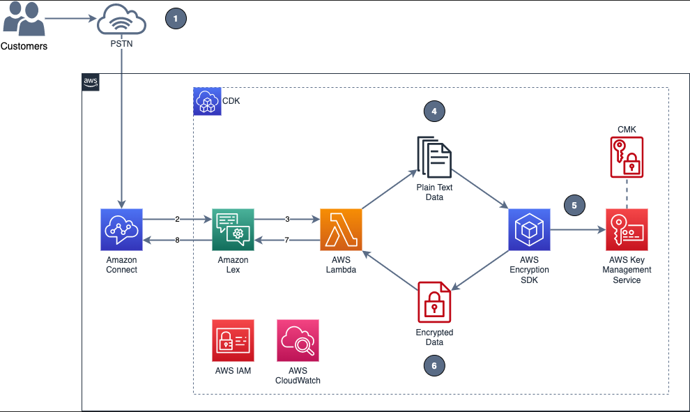
The architecture of the solution is outlined in Figure 1. The solution takes advantage of the native integration available between AWS WAF and CloudWatch, which simplifies the setup and management of this solution.
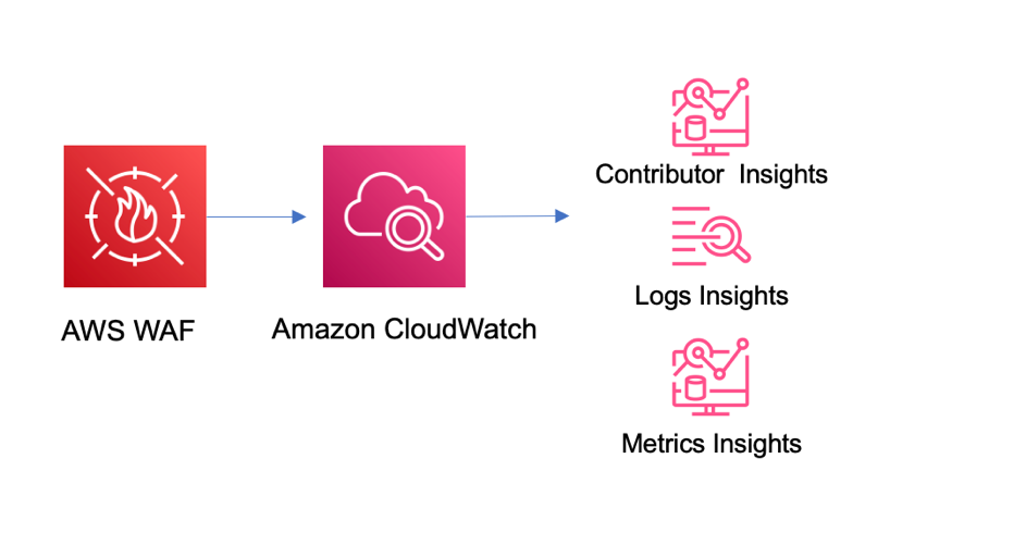
Figure 1: Solution architecture
In the solution, the logs are sent to CloudWatch (when you enable log delivery). From there, they’re ready to be consumed by all the different service options that CloudWatch offers, including the ones that we’ll use in this solution: CloudWatch Logs Insights and Contributor Insights.
Deploy the solution
Choose the following Launch stack button to launch the CloudFormation stack in your account.
![]()
You’ll be redirected to the CloudFormation service in the AWS US East (N. Virginia) Region, which is the default Region to deploy this solution, although this can vary depending on where your web ACL is located. You can change the Region as preferred. The template will spin up multiple cloud resources, such as the following:
- CloudWatch Logs Insights queries
- CloudWatch Contributor Insights visuals
- CloudWatch dashboard
The solution is quickly deployed to your account and is ready to use in less than 30 minutes. You can use the solution when the status of the stack changes to CREATE_COMPLETE.
As a measure to control costs, you can also choose whether to create the Contributor Insights rules and enable them by default. For more information on costs, see the Cost considerations section later in this post.
Explore and validate the dashboard
When the CloudFormation stack is complete, you can choose the Output tab in the CloudFormation console and then choose the dashboard link. This will take you to the CloudWatch service in the AWS Management Console. The dashboard time range presents information for the last hour of activity by default, and can go up to one week, but keep in mind that Contributor Insights has a maximum time range of 24 hours. You can also select a different dashboard refresh interval from 10 seconds up to 15 minutes.
The dashboard provides the following information from CloudWatch.
| Rule name | Description |
| WAF_top_terminating_rules | This rule shows the top rules where the requests are being terminated by AWS WAF. This can help you understand the main cause of blocked requests. |
| WAF_top_ips | This rule shows the top source IPs for requests. This can help you understand if the traffic and activity that you see is spread across many IPs or concentrated in a small group of IPs. |
| WAF_top_countries | This rule shows the main source countries for the IPs in the requests. This can help you visualize where the traffic is originating. |
| WAF_top_user_agents | This rule shows the main user agents that are being used to generate the requests. This will help you isolate problematic devices or identify potential false positives. |
| WAF_top_uri | This rule shows the main URIs in the requests that are being evaluated. This can help you identify if one specific path is the target of activity. |
| WAF_top_http | This rule shows the HTTP methods used for the requests examined by AWS WAF. This can help you understand the pattern of behavior of the traffic. |
| WAF_top_referrer_hosts | This rule shows the main referrer from which requests are being sent. This can help you identify incorrect or suspicious origins of requests based on the known application flow. |
| WAF_top_rate_rules | This rule shows the main rate rules being applied to traffic. It helps understand volumetric activity identified by AWS WAF. |
| WAF_top_labels | This rule shows the top labels found in logs. This can help you visualize the main rules that are matching on the requests evaluated by AWS WAF. |
The dashboard also provides the following information from the default CloudWatch metrics sent by AWS WAF.
| Rule name | Description |
| AllowedvsBlockedRequests | This metric shows the number of all blocked and allowed requests. This can help you understand the number of requests that AWS WAF is actively blocking. |
| Bot Requests vs non-Bot requests | This visual shows the number of requests identified as bots versus non-bots (if you’re using AWS WAF Bot Control). |
| All Requests | This metric shows the number of all requests, separated by bot and non-bot origin. This can help you understand all requests that AWS WAF is evaluating. |
| CountedRequests | This metric shows the number of all counted requests. This can help you understand the requests that are matching a rule but not being blocked, and aid the decision of a configuration change during the testing phase. |
| CaptchaRequests | This metric shows requests that go through the CAPTCHA rule. |
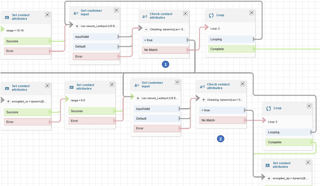
Figure 2 shows an example of how the CloudWatch dashboard displays the data within this solution. You can rearrange and customize the elements within the dashboard as needed.

You can review each of the queries and rules deployed with this solution. You can also customize these baseline queries and rules to provide more detailed information or to add custom queries and rules to the solution code. For more information on how to build queries and use CloudWatch Logs and Contributor Insights, see the CloudWatch documentation.
Use the dashboard for monitoring
After you’ve set up the dashboard, you can monitor the activity of the sites that are protected by AWS WAF. If suspicious activity is reported, you can use the visuals to understand the traffic in more detail, and drive incident response actions as needed.
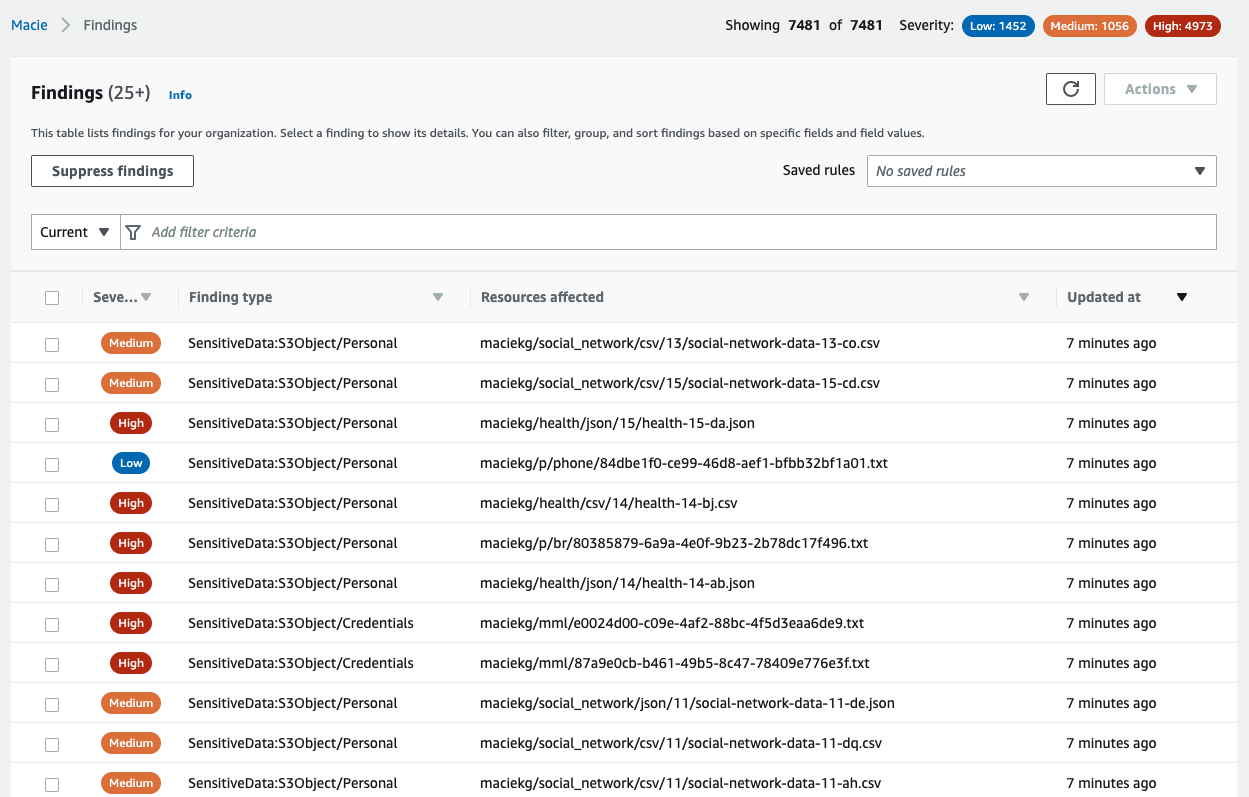
Let’s consider an example of how to use your new dashboard and its data to drive security operations decisions. Suppose that you have a website that sells custom clothing at a bargain price. It has a sign-up link to receive offers, and you’re getting reports of unusual activity by the application team. By looking at the metrics for the web ACL that protects the site, you can see the main country for source traffic and the contributing URIs, as shown in Figure 3. You can also see that most of the activity is being detected by rules that you have in place, so you can set the rules to block traffic, or if they are already blocking, you can just monitor the activity.

You can use the same visuals to decide whether an AWS WAF rule with high activity can be changed to autoblock suspicious web traffic without affecting valid customer traffic. By looking at the top terminating rules and cross-referencing information, such as source IPs, user agents, top URIs, and other request identifiers, you can understand the traffic pattern and activity of different applications and endpoints. From here, you can investigate further by using specific queries with CloudWatch Logs Insights.
Operational and security management with CloudWatch Logs Insights
You can use CloudWatch Logs Insights to interactively search and analyze log data in Amazon CloudWatch Logs using advanced queries to effectively investigate operational issues and security incidents.
Examine a bot reported as a false positive
You can use CloudWatch Logs Insights to identify requests that have specific labels to understand where the traffic is originating from based on source IP address and other essential event details. A simple example is investigating requests flagged as potential false positives.
Imagine that you have a reported false positive request that was flagged as a non-browser by AWS WAF Bot Control. You can run the non-browser user agent query that was created by the provided template on CloudWatch Logs Insights, as shown in the following example, and then verify the source IPs for the top hits for this rule group. Or you can look for a specific request that has been flagged as a false positive, in order to review the details and make adjustments as needed.
The non-browser user agent query also allows you confirm whether this request has other rule hits that were in count mode and were non-terminating; you can do this by examining the labels. If there are multiple rules matching the requests, that can be an indicator of suspicious activity.
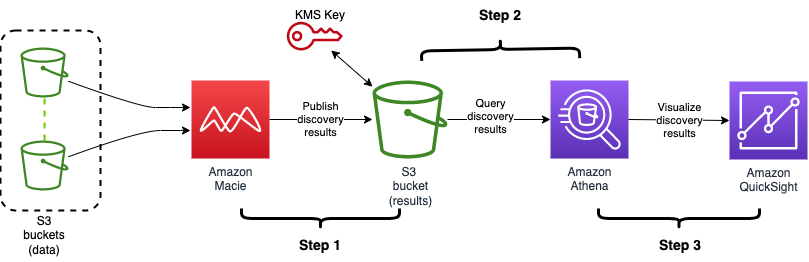
If you have a CAPTCHA challenge configured on the endpoint, you can also look at CAPTCHA responses. The CaptchaTokenqueryDefinition query provided in this solution uses a variation of the preceding format, and can display the main IPs from which bad tokens are being sent. An example query is shown following, along with the query results in Figure 4. If you have signals from non-browser user agents and CAPTCHA tokens missing, then that is a strong indicator of suspicious activity.
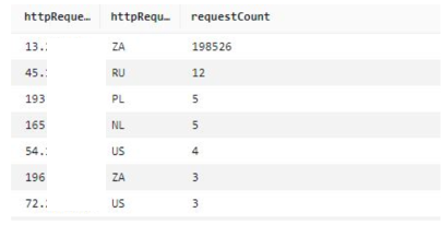
Figure 4: Main IP addresses and number of counts for CAPTCHA responses
This information can provide an indication of the main source of activity. You can then use other visuals, like top user agents or top referrers, to provide more context to the information and inform further actions, such as adding new rules to the AWS WAF configuration.
You can adapt the queries provided in the sample solution to other use cases by using the fields provided in the left-hand pane of CloudWatch Logs Insights.
Cost considerations
Configuring AWS WAF to send logs to Amazon CloudWatch logs doesn’t have an additional cost. The cost incurred is for the use of the CloudWatch features and services, such as log storage and retention, Contributor Insights rules enabled, Logs Insights queries run, matched log events, and CloudWatch dashboards. For detailed information on the pricing of these features, see the CloudWatch Logs pricing information. You can also get an estimate of potential costs by using the AWS pricing calculator for CloudWatch.
One way to help offset the cost of CloudWatch features and services is to restrict the use of the dashboard and enforce a log retention policy for AWS WAF that makes it cost effective. If you use the queries and monitoring only as-needed, this can also help reduce costs. By limiting the running of queries and the matched log events for the Contributor Insights rules, you can enable the rules only when you need them. AWS WAF also provides the option to filter the logs that are sent when logging is enabled. For more information, see AWS WAF log filtering.
Conclusion
In this post, you learned how to use a pre-built CloudWatch dashboard to monitor AWS WAF activity by using metrics and Contributor Insights rules. The dashboard can help you identify traffic patterns and activity, and you can use the sample Logs Insights queries to explore the log information in more detail and examine false positives and suspicious activity, for rule tuning.
For more information on AWS WAF and the features mentioned in this post, see the AWS WAF documentation.
If you have feedback about this post, submit comments in the Comments section below. If you have questions about this post, start a new thread on AWS WAF re:Post.
Want more AWS Security news? Follow us on Twitter.


 Stephen Said is a Senior Solutions Architect and works with Digital Native Businesses. His areas of interest are data analytics, data platforms and cloud-native software engineering.
 Vishwanatha Nayak is a Senior Solutions Architect at AWS. He works with large enterprise customers helping them design and build secure, cost-effective, and reliable modern data platforms using the AWS cloud. He is passionate about technology and likes sharing knowledge through blog posts and twitch sessions.
 Paul Villena is an Analytics Solutions Architect with expertise in building modern data and analytics solutions to drive business value. He works with customers to help them harness the power of the cloud. His areas of interests are infrastructure-as-code, serverless technologies and coding in Python.


 Aarthi Srinivasan is a Senior Big Data Architect with AWS Lake Formation. She likes building data lake solutions for AWS customers and partners. When not on the keyboard, she explores the latest science and technology trends and spends time with her family.
 Srividya Parthasarathy is a Senior Big Data Architect on the AWS Lake Formation team. She enjoys building analytics and data mesh solutions on AWS and sharing them with the community.