Post Syndicated from Scott Ward original https://aws.amazon.com/blogs/security/use-amazon-inspector-to-manage-your-build-and-deploy-pipelines-for-containerized-applications/
Amazon Inspector is an automated vulnerability management service that continually scans Amazon Web Services (AWS) workloads for software vulnerabilities and unintended network exposure. Amazon Inspector currently supports vulnerability reporting for Amazon Elastic Compute Cloud (Amazon EC2) instances and container images stored in Amazon Elastic Container Registry (Amazon ECR).
With the emergence of Docker in 2013, container technology has quickly moved from the experimentation phase into a viable production tool. Many customers are using containers to modernize their existing applications or as the foundations for new applications or services that they build. In this blog post, we’ll explore the process that Amazon Inspector takes to scan container images. We’ll also show how you can integrate Amazon Inspector into your containerized application build and deployment pipeline, and control pipeline steps based on the results of an Amazon Inspector container image scan.
Solution overview and walkthrough
The solution outlined in this post covers a deployment pipeline modeled in AWS CodePipeline. The source for the pipeline is AWS CodeCommit, and the build of the container image is performed by AWS CodeBuild. The solution uses a collection of AWS Lambda functions and an Amazon DynamoDB table to evaluate the container image status and make an automated decision about deploying the container image. Finally, the pipeline has a deploy stage that will deploy the container image into an Amazon Elastic Container Service (Amazon ECS) cluster. In this section, I’ll outline the key components of the solution and how they work. In the following section, Deploy the solution, I’ll walk you through how to actually implement the solution.
Although this solution uses AWS continuous integration and continuous delivery (CI/CD) services such as CodePipeline and CodeBuild, you can also build similar capabilities by using third-party CI/CD solutions. In addition to CodeCommit, other third-party code repositories such as GitHub or Amazon Simple Storage Service (Amazon S3) can be substituted in as a source for the pipeline.
Solution architecture
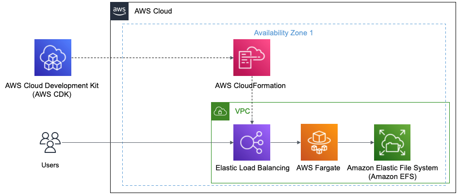
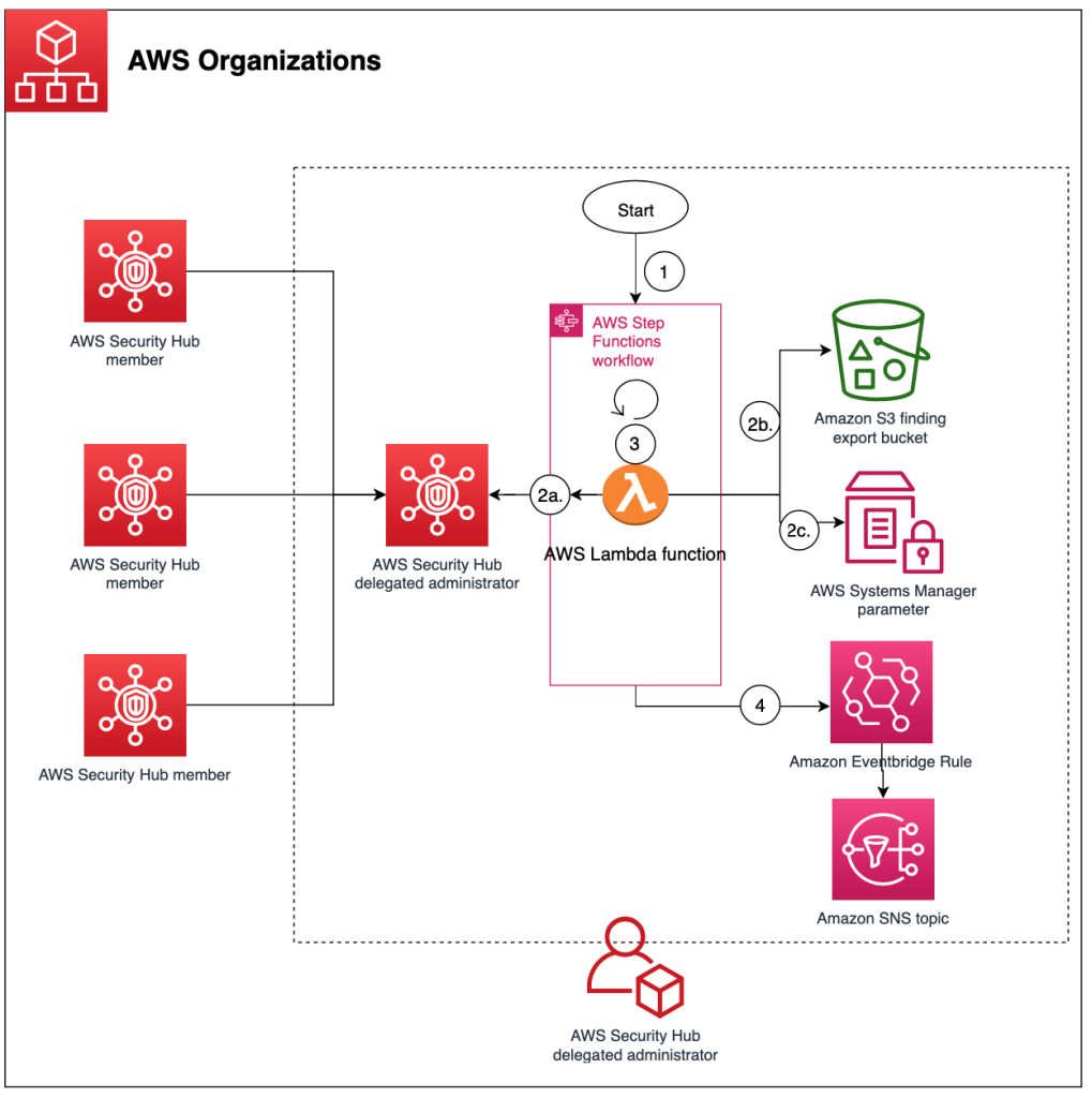
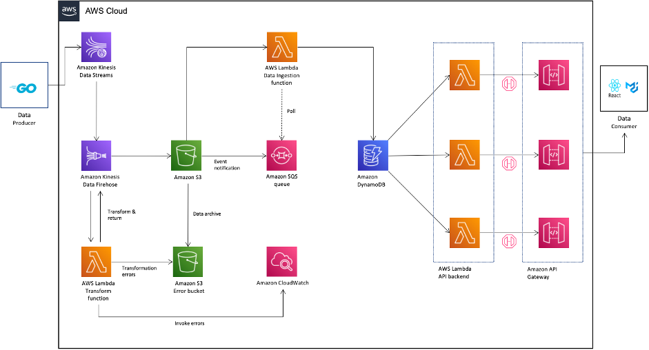
Figure 1 shows the high-level architecture of the solution, which integrates Amazon Inspector into a container build and deploy pipeline.
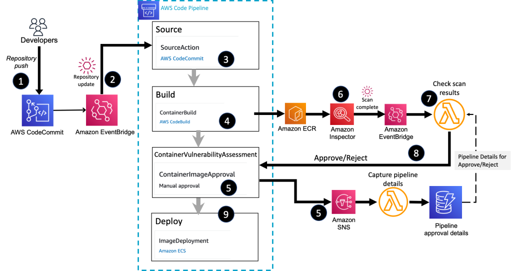
Figure 1: Overall container build and deploy architecture
The high-level workflow is as follows:
- You commit the image definition to a CodeCommit repository.
- An Amazon EventBridge rule detects the repository commit and initiates the container pipeline.
- The source stage of the pipeline pulls the image definition and build instructions from the CodeCommit repository.
- The build stage of the pipeline creates the container image and stores the final image in Amazon ECR.
- The ContainerVulnerabilityAssessment stage sends out a request for approval by using an Amazon Simple Notification Service (Amazon SNS) topic. A Lambda function associated with the topic stores the details about the container image and the active pipeline, which will be needed in order to send a response back to the pipeline stage.
- Amazon Inspector scans the Amazon ECR image for vulnerabilities.
- The Lambda function receives the Amazon Inspector scan summary message, through EventBridge, and makes a decision on allowing the image to be deployed. The function retrieves the pipeline approval details so that the approve or reject message is sent to the correct active pipeline stage.
- The Lambda function submits an Approved or Rejected status to the deployment pipeline.
- CodePipeline deploys the container image to an Amazon ECS cluster and completes the pipeline successfully if an approval is received. The pipeline status is set to Failed if the image is rejected.
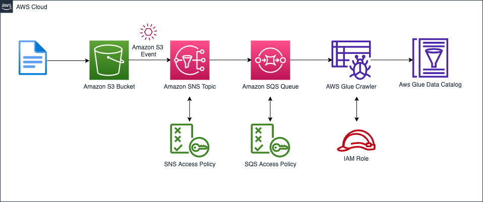
Container image build stage
Let’s now review the build stage of the pipeline that is associated with the Amazon Inspector container solution. When a new commit is made to the CodeCommit repository, an EventBridge rule, which is configured to look for updates to the CodeCommit repository, initiates the CodePipeline source action. The source action then collects files from the source repository and makes them available to the rest of the pipeline stages. The pipeline then moves to the build stage.
In the build stage, CodeBuild extracts the Dockerfile that holds the container definition and the buildspec.yaml file that contains the overall build instructions. CodeBuild creates the final container image and then pushes the container image to the designated Amazon ECR repository. As part of the build, the image digest of the container image is stored as a variable in the build stage so that it can be used by later stages in the pipeline. Additionally, the build process writes the name of the container URI, and the name of the Amazon ECS task that the container should be associated with, to a file named imagedefinitions.json. This file is stored as an artifact of the build and will be referenced during the deploy phase of the pipeline.
Now that the image is stored in an Amazon ECR repository, Amazon Inspector scanning begins to check the image for vulnerabilities.
The details of the build stage are shown in Figure 2.
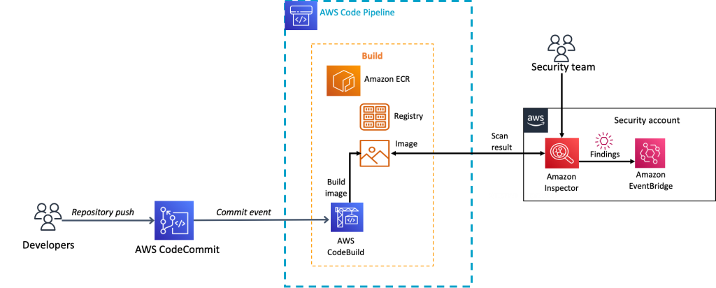
Figure 2: The container build stage
Container image approval stage
After the build stage is completed, the ContainerVulnerabilityAssessment stage begins. This stage is lightweight and consists of one stage action that is focused on waiting for an Approved or Rejected message for the container image that was created in the build stage. The ContainerVulnerabilityAssessment stage is configured to send an approval request message to an SNS topic. As part of the approval request message, the container image digest, from the build stage, will be included in the comments section of the message. The image digest is needed so that approval for the correct container image can be submitted later. Figure 3 shows the comments section of the approval action where the container image digest is referenced.
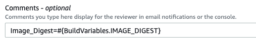
Figure 3: Container image digest reference in approval action configuration
The SNS topic that the pipeline approval message is sent to is configured to invoke a Lambda function. The purpose of this Lambda function is to pull key details from the SNS message. Details retrieved from the SNS message include the pipeline name and stage, stage approval token, and the container image digest. The pipeline name, stage, and approval token are needed so that an approved or rejected response can be sent to the correct pipeline. The container image digest is the unique identifier for the container image and is needed so that it can be associated with the correct active pipeline. This information is stored in a DynamoDB table so that it can be referenced later when the step that assesses the result of an Amazon Inspector scan submits an approved or rejected decision for the container image. Figure 4 illustrates the flow from the approval stage through storing the pipeline approval data in DynamoDB.
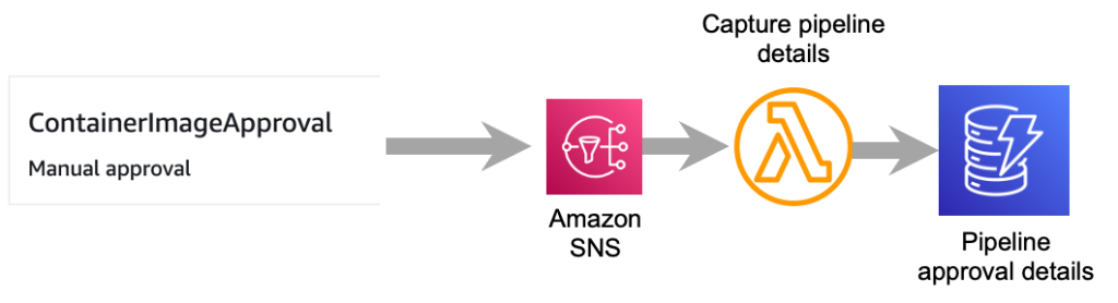
Figure 4: Flow to capture container image approval details
This approval action will remain in a pending status until it receives an Approved or Rejected message or the timeout limit of seven days is reached. The seven-day timeout for approvals is the default for CodePipeline and cannot be changed. If no response is received in seven days, the stage and pipeline will complete with a Failed status.
Amazon Inspector and container scanning
When the container image is pushed to Amazon ECR, Amazon Inspector scans it for vulnerabilities.
In order to show how you can use the findings from an Amazon Inspector container scan in a build and deploy pipeline, let’s first review the workflow that occurs when Amazon Inspector scans a container image located in Amazon ECR.
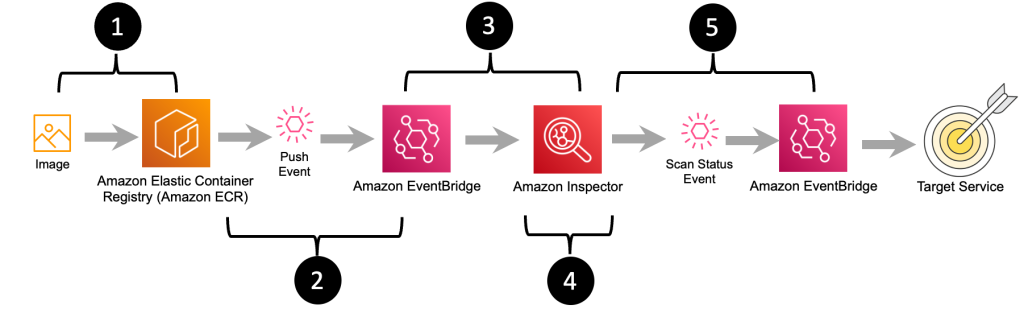
Figure 5: Image push, scan, and notification workflow
The workflow diagram in Figure 5 outlines the steps that happen after an image is pushed to Amazon ECR all the way to messaging that the image has been successfully scanned and what the final scan results are. The steps in this workflow are as follows:
- The final container image is pushed to Amazon ECR by an individual or as part of a build.
- Amazon ECR sends a message indicating that a new image has been pushed.
- The message about the new image is received by Amazon Inspector.
- Amazon Inspector pulls a copy of the container image from Amazon ECR and performs a vulnerability scan.
- When Amazon Inspector is done scanning the image, a message summarizing the severity of vulnerabilities that were identified during the container image scan is sent to Amazon EventBridge. You can create EventBridge rules that match the vulnerability summary message to route the message onto a target for notifications or to enable further action to be taken.
Here’s a sample EventBridge pattern that matches the scan summary message from Amazon Inspector.
{
  "detail-type": ["Inspector2 Scan"],
  "source": ["aws.inspector2"]
}
This entire workflow, from ingesting the initial image to sending out the status on the Amazon Inspector scan, is fully managed. You just focus on how you want to use the Amazon Inspector scan status message to govern the approval and deployment of your container image.
The following is a sample of what the Amazon Inspector vulnerability summary message looks like. Note, in bold, the container image Amazon Resource Name (ARN), image repository ARN, message detail type, image digest, and the vulnerability summary.
Processing Amazon Inspector scan results
After Amazon Inspector sends out the scan status event, a Lambda function receives and processes that event. This function needs to consume the Amazon Inspector scan status message and make a decision about whether the image can be deployed.
The eval_container_scan_results Lambda function serves two purposes: The first is to extract the findings from the Amazon Inspector scan message that invoked the Lambda function. The second is to evaluate the findings based on thresholds that are defined as parameters in the Lambda function definition. Based on the threshold evaluation, the container image will be flagged as either Approved or Rejected. Figure 6 shows examples of thresholds that are defined for different Amazon Inspector vulnerability severities, as part of the Lambda function.
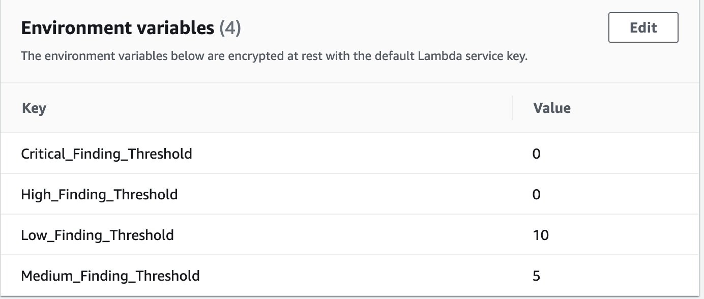
Figure 6: Vulnerability thresholds defined in Lambda environment variables
Based on the container vulnerability image results, the Lambda function determines whether the image should be approved or rejected for deployment. The function will retrieve the details about the current pipeline that the image is associated with from the DynamoDB table that was populated by the image approval action in the pipeline. After the details about the pipeline are retrieved, an Approved or Rejected message is sent to the pipeline approval action. If the status is Approved, the pipeline continues to the deploy stage, which will deploy the container image into the defined environment for that pipeline stage. If the status is Rejected, the pipeline status is set to Rejected and the pipeline will end.
Figure 7 highlights the key steps that occur within the Lambda function that evaluates the Amazon Inspector scan status message.
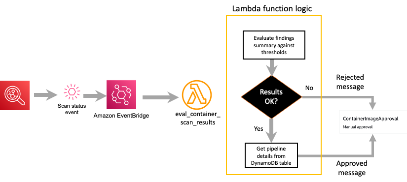
Figure 7: Amazon Inspector scan results decision
Image deployment stage
If the container image is approved, the final image is deployed to an Amazon ECS cluster. The deploy stage of the pipeline is configured with Amazon ECS as the action provider. The deploy action contains the name of the Amazon ECS cluster and stage that the container image should be deployed to. The image definition file (imagedefinitions.json) that was created in the build stage is also listed in the deploy configuration. When the deploy stage runs, it will create a revision to the existing Amazon ECS task definition. This task definition contains the name of the Amazon ECR image that has been approved for deployment. The task definition is then deployed to the Amazon ECS cluster and service.
Deploy the solution
Now that you have an understanding of how the container pipeline solution works, you can deploy the solution to your own AWS account. This section will walk you through the steps to deploy the container approval pipeline, and show you how to verify that each of the key steps is working.
Step 1: Activate Amazon Inspector in your AWS account
The sample solution provided by this blog post requires that you activate Amazon Inspector in your AWS account. If this service is not activated in your account, learn more about the free trial and pricing for this service, and follow the steps in Getting started with Amazon Inspector to set up the service and start monitoring your account.
Step 2: Deploy the AWS CloudFormation template
For this next step, make sure you deploy the template within the AWS account and AWS Region where you want to test this solution.
To deploy the CloudFormation stack
- Choose the following Launch Stack button to launch a CloudFormation stack in your account. Use the AWS Management Console navigation bar to choose the region you want to deploy the stack in.

- Review the stack name and the parameters for the template. The parameters are pre-populated with the necessary values, and there is no need to change them.
- Scroll to the bottom of the Quick create stack screen and select the checkbox next to I acknowledge that AWS CloudFormation might create IAM resources.
- Choose Create stack. The deployment of this CloudFormation stack will take 3–5 minutes.
After the CloudFormation stack has deployed successfully, you can proceed to reviewing and interacting with the deployed solution.
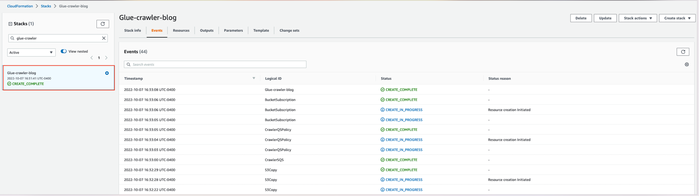
Step 3: Review the container pipeline and supporting resources
The CloudFormation stack is designed to deploy a collection of resources that will be used for an initial container build. When the CodePipeline resource is created, it will automatically pull the assets from the CodeCommit repository and start the pipeline for the container image.
To review the pipeline and resources
- In the CodePipeline console, navigate to the Region that the stack was deployed in.
- Choose the pipeline named ContainerBuildDeployPipeline to show the full pipeline details.
- Review the Source and Build stage, which will show a status of Succeeded.
- Review the ContainerVulnerabilityAssessment stage, which will show as failed with a Rejected status in the Manual Approval step.
Figure 8 shows the full completed pipeline.

Figure 8: Rejected container pipeline
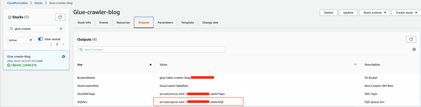
- Choose the Details link in the Manual Approval stage to reveal the reasons for the rejection. An example review summary is shown in Figure 9.

Figure 9: Container pipeline approval rejection


Review findings in Amazon Inspector (Optional)
You can use the Amazon Inspector console to see the full findings detail for this container image, if needed.
To view the findings in Amazon Inspector
- In the Amazon Inspector console, under Findings, choose By repository.
- From the list of repositories, choose the inspector-blog-images repository.
- Choose the Image tag link to bring up a list of the individual vulnerabilities that were found within the container image. Figure 10 shows an example of the vulnerabilities list in the findings details.
Figure 10: Container image findings in Amazon Inspector

Step 4: Adjust the Amazon ECS desired count for the cluster service
Up to this point, you’ve deployed a pipeline to build and validate the container image, and you’ve seen an example of how the pipeline handles a container image that did not meet the defined vulnerability thresholds. Now you’ll deploy a new container image that will pass a vulnerability assessment and complete the pipeline.
The Amazon ECS service that the CloudFormation template deploys is initially created with the number of desired tasks set to 0. In order to allow the container pipeline to successfully deploy a container, you need to update the desired tasks value.
To adjust the task count in Amazon ECS (console)
- In the Amazon ECS console, choose the link for the cluster, in this case InspectorBlogCluster.
- On the Services tab, choose the link for the service named InspectorBlogService.
- Choose the Update button. On the Configure service page, set Number of tasks to 1.
- Choose Skip to review, and then choose Update Service.
To adjust the task count in Amazon ECS (AWS CLI)
Alternatively, you can run the following AWS CLI command to update the desired task count to 1. In order to run this command, you need the ARN of the Amazon ECS cluster, which you can retrieve from the Output tab of the CloudFormation stack that you created. You can run this command from the command line of an environment of your choosing, or by using AWS CloudShell. Make sure to replace <Cluster ARN> with your own value.
$ aws ecs update-service --cluster <Cluster ARN> --service InspectorBlogService --desired-count 1
Step 5: Build and deploy a new container image
Deploying a new container image will involve pushing an updated Dockerfile to the ContainerComponentsRepo repository in CodeCommit. With CodeCommit you can interact by using standard Git commands from a command line prompt, and there are multiple approaches that you can take to connect to the AWS CodeCommit repository from the command line. For this post, in order to simplify the interactions with CodeCommit, you will be shown how to add an updated file directly through the CodeCommit console.
To add an updated Dockerfile to CodeCommit
- In the CodeCommit console, choose the repository named ContainerComponentsRepo.
- In the screen listing the repository files, choose the Dockerfile file link and choose Edit.
- In the Edit a file form, overwrite the existing file contents with the following command:
FROM public.ecr.aws/amazonlinux/amazonlinux:latest - In the Commit changes to main section, fill in the following fields.
- Author name: your name
- Email address: your email
- Commit message: ‘Updated Dockerfile’
Figure 11 shows what the completed form should look like.
Figure 11: Complete CodeCommit entry for an updated Dockerfile
- Choose Commit changes to save the new Dockerfile.

This update to the Dockerfile will immediately invoke a new instance of the container pipeline, where the updated container image will be pulled and evaluated by Amazon Inspector.
Step 6: Verify the container image approval and deployment
With a new pipeline initiated through the push of the updated Dockerfile, you can now review the overall pipeline to see that the container image was approved and deployed.
To see the full details in CodePipeline
- In the CodePipeline console, choose the container-build-deploy pipeline. You should see the container pipeline in an active status. In about five minutes, you should see the ContainerVulnerabilityAssessment stage move to completed with an Approved status, and the deploy stage should show a Succeeded status.
- To confirm that the final image was deployed to the Amazon ECS cluster, from the Deploy stage, choose Details. This will open a new browser tab for the Amazon ECS service.
- In the Amazon ECS console, choose the Tasks tab. You should see a task with Last status showing RUNNING. This is confirmation that the image was successfully approved and deployed through the container pipeline. Figure 12 shows where the task definition and status are located.
Figure 12: Task status after deploying the container image
- Choose the task definition to bring up the latest task definition revision, which was created by the deploy stage of the container pipeline.
- Scroll down in the task definition screen to the Container definitions section. Note that the task is tied to the image you deployed, providing further verification that the approved container image was successfully deployed. Figure 13 shows where the container definition can be found and what you should expect to see.
Figure 13: Container associated with revised task definition


Clean up the solution
When you’re finished deploying and testing the solution, use the following steps to remove the solution stack from your account.
To delete images from the Amazon ECR repository
- In the Amazon ECR console, navigate to the AWS account and Region where you deployed the solution.
- Choose the link for the repository named inspector-blog-images.
- Delete all of the images that are listed in the repository.
To delete objects in the CodePipeline artifact bucket
- In the Amazon S3 console in your AWS account, locate the bucket whose name starts with blog-base-setup-codepipelineartifactstorebucket.
- Delete the ContainerBuildDeploy folder that is in the bucket.
To delete the CloudFormation stack
- In the CloudFormation console, delete the CloudFormation stack that was created to perform the steps in this post.
Conclusion
This post describes a solution that allows you to build your container images, have the images scanned for vulnerabilities by Amazon Inspector, and use the output from Amazon Inspector to determine whether the image should be allowed to be deployed into your environments.
This solution represents a pipeline with very simple build and deploy stages. Your pipeline will vary and may consist of multiple test stages and deployment stages for multiple environments. Additionally, the logic you use to determine whether a container image should be deployed may be different. The contents of this blog post are intended to help serve as a foundation that you can build on as you decide how to use Amazon Inspector for container vulnerability scanning. Feel free to use this guidance, and the example we provided, to extend the solution into your specific deployment pipeline.
If you have questions, contact AWS Support, or start a new thread on the AWS re:Post Amazon Inspector Forum. If you have feedback about this post, submit comments in the Comments section below.
Want more AWS Security news? Follow us on Twitter.


 Ying Wang is a Manager of Software Development Engineer. She has 12 years of expertise in data analytics and science. She assisted customers with enterprise data architecture solutions to scale their data analytics in the cloud during her time as a data architect. Currently, she helps customer to unlock the power of Data with QuickSight from engineering by delivering new features.
 Ian Liao is a Senior Data Visualization Architect at AWS Professional Services. Before AWS, Ian spent years building startups in data and analytics. Now he enjoys helping customer to scale their data application on the cloud.
 Maitri Brahmbhatt is a Business Intelligence Engineer at AWS. She helps customers and partners leverage their data to gain insights into their business and make data driven decisions by developing QuickSight dashboards.
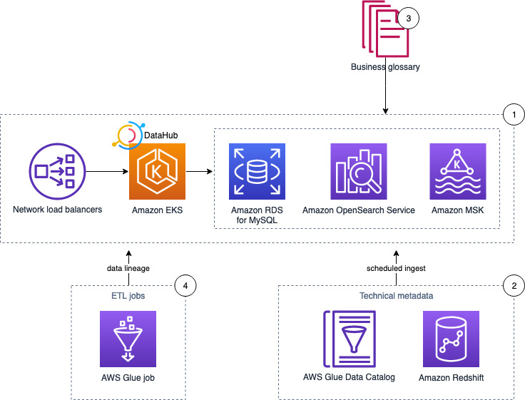


 Moustafa Mahmoud is a Solutions Architect of AWS Data Lab with a passion for data integration, data analysis, machine learning, and BI. Moustafa helps customers convert their ideas to a production-ready data product on AWS. He has over 10 years of experience as a data engineer, machine learning practitioner, and software developer. In his spare time, Moustafa loves exploring nature, reading, and spending time with friends and family.
 Corvus Lee is a Solutions Architect of AWS Data Lab. He enjoys all kinds of data-related discussions, and helps customers build MVPs using AWS Databases, Analytics, and Machine Learning services.


 For this specific example, we use the following information for our Azure SQL Instance: