Tag Archives: serverless

Chaos experiments using AWS Step Functions and AWS Fault Injection Simulator

Post Syndicated from James Beswick original https://aws.amazon.com/blogs/compute/chaos-experiments-using-aws-step-functions-and-aws-fault-injection-simulator/

This post is written by Arunsingh Jeyasingh Jacob, Senior Solutions Architect, and Sindhura Palakodety, Senior Solutions Architect.

To run business-critical applications at scale, it is important to determine the resiliency of the application. Chaos experiments induce controlled failures into a distributed application to gain confidence in the application behavior. The learnings from these experiments can be fed into a continuous feedback cycle to improve the resiliency.

In 2021, AWS launched AWS Fault Injection Simulator (FIS). This is a fully managed service for running Fault Injection experiments on AWS. It makes it easier to improve an application’s performance, observability, and resiliency. With Fault Injection Simulator, AWS customers can quickly set up experiments using pre-built templates that generate the desired disruptions.

Overview

This post uses AWS Step Functions to create and run AWS Fault Injection Simulator (FIS) experiments. You are encouraged to perform these experiments in a test account. Do not use the example in a production environment without making appropriate code changes.

The demo-fis-stepfunctions code deployed in this post is used to build the Step Functions state machine for FIS experiments.

There are two Step Functions workflows that are deployed. One is for chaos testing Amazon EC2 workloads and the other one is for Amazon ECS workloads.

The Step Functions workflow for EC2 workloads

The following Step Functions workflow shows an EC2 chaos experiment to stress CPU utilization, and stop and terminate EC2 instances.

Step Functions workflow for Amazon EC2 Fault Injection Experiments

EC2 experiment templates

This workflow runs through FIS experiment template creation followed by the execution of the FIS experiment. The FIS experiment template contains one or more actions to run on specified targets during an experiment. By creating a template, you are not running experiments against any workload, but creating a definition for the experiment.

The EC2 experiment templates created in this workflow are:

  • EC2CPUStressExperimentTemplate
  • EC2StopExperimentTemplate
  • EC2TerminateExperimentTemplate

These are the terms used in the FIS experiment template:

  • Actions: While creating an experimentation template, you must define an action once during an experiment.
  • Targets: A target is one or more AWS resources on which an action is performed by AWS Fault Injection Simulator (AWS FIS) during an experiment. For example, defining which instances to stress CPUs based on the tags.
  • Filters: Resource filters are queries that identify target resources according to specific attributes.
  • IAM role: This IAM role is assumed by FIS to perform the actions mentioned in the template. The Step Functions role must pass permissions to this FIS role.
  • Client token: The Step Functions execution fails if a client token is not passed.
  • Selection mode: Run experiments on all the resources matching the target criteria or specify the number of resources. For example, the EC2CPUStressExperimentTemplate targets one resource in random.

The ‘EC2CPUStressExperimentTemplate’ code defines how to stop EC2 instances with the tag ‘FISAction: CPUStress’:

{
   "Targets": {
      "CPUStressInstances": {
         "ResourceType": "aws:ec2:instance",
         "ResourceTags": {
            "FISAction": "CPUStress"
         },
         "Filters": [
            {
               "Path": "VpcId",
               "Values": [
                  "${VpcID}"
               ]
            }
         ],
         "SelectionMode": "COUNT(1)"
      }
   }
}

Targets can also be filtered using parameters like Amazon VPC ID. You can change the Step Functions definition by modifying the targets, actions, and filters.

EC2 FIS experiments

FIS experiment uses the experiment template definition during the state execution, and targets the appropriate resources.

  1. There are three EC2 FIS experiments created as a part of the workflow:1. CPUStressInstances: This runs after the ‘EC2CPUStressExperimentTemplate’ state. In this state, AWS Systems Manager (SSM) attempts to add CPU stress on the target instance with the tag “FISAction: CPUStress”. You can monitor the metric in the Amazon CloudWatch dashboard, and take actions using Amazon CloudWatch alarms.
    Monitoring the CPU utilization using Amazon CloudWatch
  2. StopInstances: Here, the target instances enter the ‘stopping’ state. Based on the template definition, all the EC2 instances with the tag “FISAction:Stop” in the filtered VPC are stopped.
  3.  TerminateInstances: This terminates the target instances with the tag “FISAction:Terminate” in the filtered VPC.

The Step Functions workflow for Amazon ECS workloads

The following Step Functions workflow shows an FIS experiment to stop ECS tasks:

Step Functions workflow for Amazon ECS Fault Injection experiment

  • Amazon ECS experiment template: The ECSStopTaskExperimentTemplate state is created in this workflow. This FIS template defines the action to be run during the experiment.
  • Amazon ECS experiments: After creating the experiment template, the ECSStopTask state runs the FIS experiment.
  • ECSStopTask: FIS targets all the Amazon ECS tasks with the tag “FISAction: StopECSTask” and stops the tasks.

After the FIS experiment state is initiated, the status of the experiment can be polled before proceeding to the next state. The FIS experiments have multiple states like pending, initiating, running, completed, stopping, stopped, and failed.

The choice state in the workflow checks for the ‘running’ state by polling the status using FIS: GetExperiment API. A ‘failed’ status will result in the workflow failure. You can also design the workflow by introducing wait times between the experiments or by including flow activities like parallel.

Deploying with the AWS Serverless Application Model

This example has the following prerequisites:

  1. Create an AWS account if you don’t have one already.
  2. A valid existing VPC with subnets.
  3. A local install of Git CLI.
  4. A local install of AWS SAM CLI to build and deploy the sample code.

After installation, follow these steps to deploy the example:

  1. Clone the sample code:
    git clone https://github.com/aws-samples/aws-stepfunctions-examples.git
    cd sam/demo-fis-stepfunctions/
    
  2. Modify the templates as needed. You can also edit the state machine code from the AWS Management Console after you deploy this code.
  3. Build and deploy the code:
    sam build 
    sam deploy --guided
    

To learn more, visit the AWS SAM deployment documentation. This launches an AWS CloudFormation stack that creates the state machine, AWS IAM roles and CloudWatch log group. The next step is to run the state machines.

Running the Step Functions workflows

The AWS SAM deployment creates two Step Functions state machines in the deployed AWS Region: FISTest-aws-region-StateMachineFIS and FISTest-aws-region-StateMachineECSFIS.

Before running the state machine FISTest-aws-region-StateMachineFIS, create three EC2 instances with the tags “FISAction: CPUStress”, “FISAction:Stop” and “FISAction:Terminate” respectively.

  1. Navigate to the Step Functions console.
  2. Choose FISTest-aws-region-StateMachineFIS then Start execution.

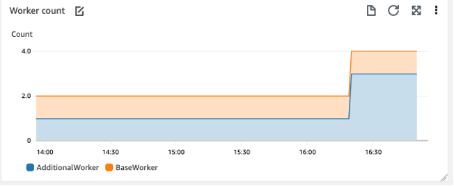
As the workflow progresses, CPU Utilization spikes in one Amazon EC2 instance. The other Amazon EC2 instances are stopped and terminated.

To run chaos experiments on an ECS cluster, you can either use an existing ECS cluster or create a new cluster. To create an ECS cluster:

  1. Navigate to the ECS console.
  2. Choose Get Started.
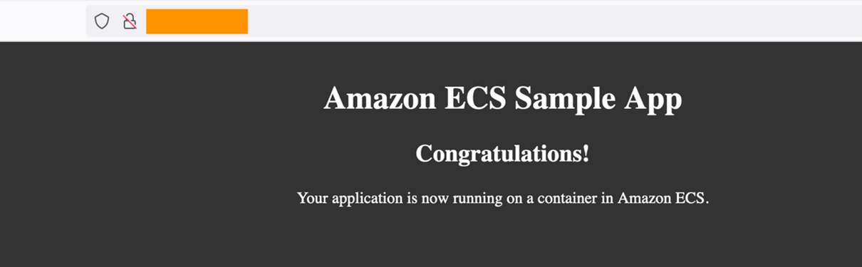
  3. Choose sample-app and follow the instructions to deploy. Wait for the cluster to be created.
  4. Choose the sample cluster, then choose Tasks.
  5. Choose the running tasks and add the tag “FISAction: StopECSTask”

From the browser, the public IP assigned to the task takes you to the sample application.

Amazon ECS Sample Application

  1. Navigate to the Step Functions console.
  2. Choose FISTest-aws-region-StateMachineECSFIS, then Start execution.
  3. The workflow transitions to Wait during the execution.

Execution - FIS Step Functions workflow for ECS experiment

Once the execution is complete, the webpage momentarily becomes unavailable until a new task comes up. The public IP address and ARN of the task changes. The task status of the stopped tasks now shows “Task stopped by AWS FIS”.

ECS Task stopped by AWS FIS Experiment

To perform an FIS experiment against an existing ECS cluster, add the Resource Tags value “FISAction: StopECSTask” to your ECS tasks before running the workflows.

{
   "Targets": {
      "ecsfargatetask": {
         "ResourceType": "aws:ecs:task",
         "ResourceTags": {
            "FISAction": "StopECSTask"
         },
         "SelectionMode": "ALL"
      }
   }
}

Cleanup

If you have deployed the code using AWS SAM, delete the resources:

sam delete –stack-name <STACK_NAME>

Refer to this documentation for further information.

Conclusion

This blog post describes how to use Step Functions to orchestrate Fault Injection Simulator (FIS) experiments for EC2 and ECS workloads. Using the workflow in this post as an example, you can build state machines for more AWS FIS experiments. Step Functions, AWS FIS, and other services can be combined to build resiliency workflows, and test your application against your resiliency goals.

To learn more about AWS FIS and Step Functions, visit:

For more Step Functions resources, visit the Serverless Workflows Collection.

Visualizing the impact of AWS Lambda code updates

Post Syndicated from David Boyne original https://aws.amazon.com/blogs/compute/visualizing-the-impact-of-aws-lambda-code-updates/

This post is written by Brigit Brown (Solutions Architect), and Helen Ashton (Observability Specialist Solutions Architect).

When using AWS Lambda, changes made to code can impact performance, functionality, and cost. It can be challenging to gain insight into how these code changes impact performance.

This blog post demonstrates how to capture, record, and visualize Lambda code deployment data with other data in an Amazon CloudWatch dashboard. This solution enables serverless developers to gain insight into the impact of code changes to Lambda functions and make data-driven decisions.

There are three steps to this solution:

  1. Capture: Lambda function code updates using Amazon EventBridge.
  2. Record: Lambda function code updates by creating an Amazon CloudWatch metric.
  3. Visualize: The relationship between Lambda function code updates and application KPIs by creating a CloudWatch dashboard.

Overview

EventBridge and CloudWatch are used to monitor and visualize the impact of code changes to Lambda functions on key application metrics.

Architecture diagram for capturing, recording, and visualizing Lambda function updates, showing the AWS Lambda function event being detected by Amazon EventBridge, and finally being sent to Amazon CloudWatch

Step 1: Capturing

AWS CloudTrail records all management events for AWS services. These are the operations performed on resources in your AWS account and include Lambda function code updates.

An EventBridge rule can listen for Lambda functions code updates and send these events to other AWS services, in this case to CloudWatch.

You can create EventBridge rules using an example event syntax as reference. To get the example event, update the code of a Lambda function and search in CloudTrail for all events with Event source of lambda.amazonaws.com, and an Event name starting with UpdateFunctionCode. UpdateFunctionCode is one of many events captured for Lambda functions. For example:

{
  "eventVersion": "1.08",
  "userIdentity": {
    "type": "AssumedRole",
    "principalId": "x",
    "arn": "arn:aws:sts::xxxxxxxxxxxx:assumed-role/Admin/x",
    "accountId": "xxxxxxxxxxxx",
    "accessKeyId": "xxxxxxxxxxxxxxxxx",
    "sessionContext": {
      "sessionIssuer": {
        "type": "Role",
        "principalId": "x",
        "arn": "arn:aws:iam::xxxxxxxxxxxx:role/Admin",
        "accountId": "xxxxxxxxxxxx",
        "userName": "Admin"
      },
      "webIdFederationData": {},
      "attributes": {
        "creationDate": "2022-09-22T16:37:04Z",
        "mfaAuthenticated": "false"
      }
    }
  },
  "eventTime": "2022-09-22T16:42:07Z",
  "eventSource": "lambda.amazonaws.com",
  "eventName": "UpdateFunctionCode20150331v2",
  "awsRegion": "us-east-1",
  "sourceIPAddress": "AWS Internal",
  "userAgent": "AWS Internal",
  "requestParameters": {
    "fullyQualifiedArn": {
      "arnPrefix": {
        "partition": "aws",
        "region": "us-east-1",
        "account": "xxxxxxxxxxxx"
      },
      "relativeId": {
        "functionName": "example-function"
      },
      "functionQualifier": {}
    },
    "functionName": "arn:aws:lambda:us-east-1:xxxxxxxxxxxx:function:example-function",
    "publish": false,
    "dryRun": false
  },
  "responseElements": {
    "functionName": "example-function",
    "functionArn": "arn:aws:lambda:us-east-1:xxxxxxxxxxxx:function:example-function",
    "runtime": "python3.8",
    "role": "arn:aws:iam::xxxxxxxxxxxx:role/role-name",
    "handler": "lambda_function.lambda_handler",
    "codeSize": 1011,
    "description": "",
    "timeout": 123,
    "memorySize": 128,
    "lastModified": "2022-09-22T16:42:07.000+0000",
    "codeSha256": "x",
    "version": "$LATEST",
    "environment": {},
    "tracingConfig": {
      "mode": "PassThrough"
    },
    "revisionId": "x",
    "state": "Active",
    "lastUpdateStatus": "InProgress",
    "lastUpdateStatusReason": "The function is being created.",
    "lastUpdateStatusReasonCode": "Creating",
    "packageType": "Zip",
    "architectures": ["x86_64"],
    "ephemeralStorage": {
      "size": 512
    }
  },
  "requestID": "f566f75f-a7a8-4e87-a177-2db001d40382",
  "eventID": "4f90175d-3063-49b4-a467-04150b418457",
  "readOnly": false,
  "eventType": "AwsApiCall",
  "managementEvent": true,
  "recipientAccountId": "113420664689",
  "eventCategory": "Management",
  "sessionCredentialFromConsole": "true"
}

The key fields are eventSource, eventName, functionName, and eventType. This is the event syntax containing only the key fields.

{
    "eventSource": "lambda.amazonaws.com",
    "eventName": "UpdateFunctionCode20150331v2",
    "responseElements": {
        "functionName": "example-function"
        }
    "eventType": "AwsApiCall",
}

Use this example event as a reference to write the EventBridge rule pattern.

{
  "source": ["aws.lambda"],
  "detail-type": ["AWS API Call via CloudTrail"],
  "detail": {
    "eventSource": ["lambda.amazonaws.com"],
    "eventName": [{
      "prefix": "UpdateFunctionCode"
    }],
    "eventType": ["AwsApiCall"]
  }
}

In this EventBridge rule, the detail section contains properties to match the original UpdateFunctionCode event pattern. The values to match are in square brackets using EventBridge syntax.

The eventName changes with each UpdateFunctionCode event, including date and version information within the value (i.e. UpdateFunctionCode20150331v2) and so a prefix matching filter is used to match the start of the eventName.

The source and the detail-type of the event are two additional fields included by EventBridge. For all Lambda CloudTrail calls, the detail-type is [“AWS API Call via CloudTrail”] and the source is “aws.lambda“.

Next, send an event to CloudWatch. Each EventBridge rule can send events to multiple targets, including Amazon SNS and CloudWatch log groups. Choose a target of CloudWatch log groups, with the log group specified as /aws/events/lambda/updates. EventBridge creates this log group in CloudWatch.

Finally, test the EventBridge rule.

  1. To trigger an event, change the code for any Lambda function and deploy.

    AWS Console

  2. To view the event, navigate to the CloudWatch console > Logs > Log groups.

    Log group


  3. Choose the log group (/aws/events/lambda/updates).

    Selected log group

  4. Select the most recent log stream.

    Recent log stream

  5. If the EventBridge rule is successful, the Lambda code update event is visible. To see the JSON from the event, expand the event with the arrows to the left and see the detail field.

    Expanded view of event

Step 2: Recording

To display the Lambda function update data alongside other CloudWatch metrics, convert the log event into a metric using metric filters. A metric filter is created on a log group. If a log event matches a metric filter, a metric data point is created.

A metric filter uses a filter pattern to match on specific fields in the JSON event. In this case, the filter pattern matches on the eventName starting with UpdateFunctionCode (note the star as a wildcard).

{ $.detail.eventName=UpdateFunctionCode* }

Create a metric filter with the following:

  • Metric namespace: LambdaEvents
  • Metric name: UpdateFunction
  • Metric value: 1
  • Dimensions: DimensionName: FunctionName; Dimension Value: $.detail.responseElements.functionName

Dimensions allow metadata to be added to metrics. Setting a dimension with the JSON path to $.detail.responseElements.functionName allows the FunctionName value to come from the data in the log event. This makes this a generic metric filter for any Lambda function.

The event pattern of a metric filter can be tested on real data in the Test pattern section. Choose the log stream to test the filter on by using the Select log data drop down and selecting Test pattern. This shows a table with the matched events and the field value.

The CloudWatch console provides a view of the metrics for Lambda functions. To see the metric data, update the code for a Lambda function and navigate to the CloudWatch console. Choose Metrics > All metrics from the left menu, the Custom namespace of LambdaEvents, and dimension of FunctionName (as set in the preceding metric filter). To see the data on the chart, check the box beside the metric of interest. The metric can be added to a CloudWatch dashboard under the Actions menu.

Metric filters only create metrics when a new log event is ingested. You must wait for a new log event to see the metrics.

Step 3: Visualizing

A CloudWatch dashboard enables the visualization of metric data and creation of customized views. The dashboard can contain multiple widgets with data from metrics, logs, and alarms.

The following dashboard shows an example of visualizing Lambda code updates alongside other performance data. There is no single visualization that is right for everyone. The data added to the dashboard depends on the questions and actions the business wants to take. This data can be varied and include performance data, KPIs, and user experience.

The dashboard displays data on Lambda function code updates and Lambda performance (duration). A metric line widget shows a time chart of Lambda function duration with the update Lambda code metric data. Duration is a performance metric that is provided for all Lambda functions. Read more in Working with Lambda Function metrics.

A CloudWatch dashboard showing visualization of Lambda update code events alongside Lambda function durations for two functions. The duration is shown as an average value for the last hour and a time chart.

This screenshot shows the Lambda function duration for two different functions: PlaceOrder and AddToBasket. The duration for each function is represented in two ways:

  • A single number showing the average duration in the last hour.
  • A chart of the duration over time.

The Lambda function update event is shown on the duration time chart as an orange dot. The different views of duration show a high-level value and the detailed behavior over time. The detailed behavior is important to understanding the outcome. With only the high-level value, it is difficult to see if an increase in the hourly duration results from a short-term increase in duration, an upward trend, or a step change in behavior.

What is clear from this dashboard is that immediately following an update to the Lambda code, the PlaceOrder function duration dramatically increases from an average of ~100ms to ~300ms. This is a step change in behavior. The same deployment does not have the same impact on the duration of the AddToBasket function. While the duration is increasing near the end of the time period, it is less clear that this is because of the deployment. This dashboard provides awareness to the impact of the change at a function level so that the business can decide if the impact is acceptable.

Resources for creating your own dashboard

Conclusion

This blog demonstrates how to create an EventBridge rule and CloudWatch dashboard to visualize the impact of Lambda function code changes on performance data. First, an EventBridge rule is created to capture Lambda function code update events recorded in CloudTrail. EventBridge sends the event to CloudWatch where UpdateFunctionCode events are stored as a metric. The UpdateFunctionCode event data is visualized in a CloudWatch dashboard alongside Lambda performance data. This visibility enables teams to better understand the impact of code changes and make data-driven solutions.

You can modify the concepts in this blog and apply them to a wide variety of use cases. EventBridge can capture AWS CodeCommit and AWS CloudFormation deployments, and send the events to a CloudWatch dashboard to visualize alongside other metrics.

For more serverless learning resources, visit Serverless Land.

Let’s Architect! Optimizing the cost of your architecture

Post Syndicated from Luca Mezzalira original https://aws.amazon.com/blogs/architecture/lets-architect-optimizing-the-cost-of-your-architecture/

Written in collaboration with Ben Moses, AWS Senior Solutions Architect, and Michael Holtby, AWS Senior Manager Solutions Architecture


Designing an architecture is not a simple task. There are many dimensions and characteristics of a solution to consider, such as the availability, performance, or resilience.

In this Let’s Architect!, we explore cost optimization and ideas on how to rethink your AWS workloads, providing suggestions that span from compute to data transfer.

Migrating AWS Lambda functions to Arm-based AWS Graviton2 processors

AWS Graviton processors are custom silicon from Amazon’s Annapurna Labs. Based on the Arm processor architecture, they are optimized for performance and cost, which allows customers to get up to 34% better price performance.

This AWS Compute Blog post discusses some of the differences between the x86 and Arm architectures, as well as methods for developing Lambda functions on Graviton2, including performance benchmarking.

Many serverless workloads can benefit from Graviton2, especially when they are not using a library that requires an x86 architecture to run.

Take me to this Compute post!

Choosing Graviton2 for AWS Lambda function in the AWS console

Choosing Graviton2 for AWS Lambda function in the AWS console

Key considerations in moving to Graviton2 for Amazon RDS and Amazon Aurora databases

Amazon Relational Database Service (Amazon RDS) and Amazon Aurora support a multitude of instance types to scale database workloads based on needs. Both services now support Arm-based AWS Graviton2 instances, which provide up to 52% price/performance improvement for Amazon RDS open-source databases, depending on database engine, version, and workload. They also provide up to 35% price/performance improvement for Amazon Aurora, depending on database size.

This AWS Database Blog post showcases strategies for updating RDS DB instances to make use of Graviton2 with minimal changes.

Take me to this Database post!

Choose your instance class that leverages Graviton2, such as db.r6g.large (the “g” stands for Graviton2)

Choose your instance class that leverages Graviton2, such as db.r6g.large (the “g” stands for Graviton2)

Overview of Data Transfer Costs for Common Architectures

Data transfer charges are often overlooked while architecting an AWS solution. Considering data transfer charges while making architectural decisions can save costs. This AWS Architecture Blog post describes the different flows of traffic within a typical cloud architecture, showing where costs do and do not apply. For areas where cost applies, it shows best-practice strategies to minimize these expenses while retaining a healthy security posture.

Take me to this Architecture post!

Accessing AWS services in different Regions

Accessing AWS services in different Regions

Improve cost visibility and re-architect for cost optimization

This Architecture Blog post is a collection of best practices for cost management in AWS, including the relevant tools; plus, it is part of a series on cost optimization using an e-commerce example.

AWS Cost Explorer is used to first identify opportunities for optimizations, including data transfer, storage in Amazon Simple Storage Service and Amazon Elastic Block Store, idle resources, and the use of Graviton2 (Amazon’s Arm-based custom silicon). The post discusses establishing a FinOps culture and making use of Service Control Policies (SCPs) to control ongoing costs and guide deployment decisions, such as instance-type selection.

Take me to this Architecture post!

Applying SCPs on different environments for cost control

Applying SCPs on different environments for cost control

See you next time!

Thanks for joining us to discuss optimizing costs while architecting! This is the last Let’s Architect! post of 2022. We will see you again in 2023, when we explore even more architecture topics together.

Wishing you a happy holiday season and joyous new year!

Can’t get enough of Let’s Architect!?

Visit the Let’s Architect! page of the AWS Architecture Blog for access to the whole series.

Looking for more architecture content?

AWS Architecture Center provides reference architecture diagrams, vetted architecture solutions, Well-Architected best practices, patterns, icons, and more!

Securing Lambda Function URLs using Amazon Cognito, Amazon CloudFront and AWS WAF

Post Syndicated from Marcia Villalba original https://aws.amazon.com/blogs/compute/securing-lambda-function-urls-using-amazon-cognito-amazon-cloudfront-and-aws-waf/

This post is written by Madhu Singh (Solutions Architect), and Krupanidhi Jay (Solutions Architect).

Lambda function URLs is a dedicated HTTPs endpoint for a AWS Lambda function. You can configure a function URL to have two methods of authentication: IAM and NONE. IAM authentication means that you are restricting access to the function URL (and in-turn access to invoke the Lambda function) to certain AWS principals (such as roles or users). Authentication type of NONE means that the Lambda function URL has no authentication and is open for anyone to invoke the function.

This blog shows how to use Lambda function URLs with an authentication type of NONE and use custom authorization logic as part of the function code, and to only allow requests that present valid Amazon Cognito credentials when invoking the function. You also learn ways to protect Lambda function URL against common security threats like DDoS using AWS WAF and Amazon CloudFront.

Lambda function URLs provides a simpler way to invoke your function using HTTP calls. However, it is not a replacement for Amazon API Gateway, which provides advanced features like request validation and rate throttling.

Solution overview

There are four core components in the example.

1. A Lambda function with function URLs enabled

At the core of the example is a Lambda function with the function URLs feature enabled with the authentication type of NONE. This function responds with a success message if a valid authorization code is passed during invocation. If not, it responds with a failure message.

2. Amazon Cognito User Pool

Amazon Cognito user pools enable user authentication on websites and mobile apps. You can also enable publicly accessible Login and Sign-Up pages in your applications using Amazon Cognito user pools’ feature called the hosted UI.

In this example, you use a user pool and the associated Hosted UI to enable user login and sign-up on the website used as entry point. This Lambda function validates the authorization code against this Amazon Cognito user pool.

3. CloudFront distribution using AWS WAF

CloudFront is a content delivery network (CDN) service that helps deliver content to end users with low latency, while also improving the security posture for your applications.

AWS WAF is a web application firewall that helps protect your web applications or APIs against common web exploits and bots and AWS Shield is a managed distributed denial of service (DDoS) protection service that safeguards applications running on AWS. AWS WAF inspects the incoming request according to the configured Web Access Control List (web ACL) rules.

Adding CloudFront in front of your Lambda function URL helps to cache content closer to the viewer, and activating AWS WAF and AWS Shield helps in increasing security posture against multiple types of attacks, including network and application layer DDoS attacks.

4. Public website that invokes the Lambda function

The example also creates a public website built on React JS and hosted in AWS Amplify as the entry point for the demo. This website works both in authenticated mode and in guest mode. For authentication, the website uses Amazon Cognito user pools hosted UI.

Solution architecture

This shows the architecture of the example and the information flow for user requests.

In the request flow:

  1. The entry point is the website hosted in AWS Amplify. In the home page, when you choose “sign in”, you are redirected to the Amazon Cognito hosted UI for the user pool.
  2. Upon successful login, Amazon Cognito returns the authorization code, which is stored as a cookie with the name “code”. The user is redirected back to the website, which has an “execute Lambda” button.
  3. When the user choose “execute Lambda”, the value from the “code” cookie is passed in the request body to the CloudFront distribution endpoint.
  4. The AWS WAF web ACL rules are configured to determine whether the request is originating from the US or Canada IP addresses and to determine if the request should be allowed to invoke Lambda function URL origin.
  5. Allowed requests are forwarded to the CloudFront distribution endpoint.
  6. CloudFront is configured to allow CORS headers and has the origin set to the Lambda function URL. The request that CloudFront receives is passed to the function URL.
  7. This invokes the Lambda function associated with the function URL, which validates the token.
  8. The function code does the following in order:
    1. Exchange the authorization code in the request body (passed as the event object to Lambda function) to access_token using Amazon Cognito’s token endpoint (check the documentation for more details).
      1. Amazon Cognito user pool’s attributes like user pool URL, Client ID and Secret are retrieved from AWS Systems Manager Parameter Store (SSM Parameters).
      2. These values are stored in SSM Parameter Store at the time these resources are deployed via AWS CDK (see “how to deploy” section)
    2. The access token is then verified to determine its authenticity.
    3. If valid, the Lambda function returns a message stating user is authenticated as <username> and execution was successful.
    4. If either the authorization code was not present, for example, the user was in “guest mode” on the website, or the code is invalid or expired, the Lambda function returns a message stating that the user is not authorized to execute the function.
  9. The webpage displays the Lambda function return message as an alert.

Getting started

Pre-requisites:

Before deploying the solution, please follow the README from the GitHub repository and take the necessary steps to fulfill the pre-requisites.

Deploy the sample solution

1. From the code directory, download the dependencies:

$ npm install

2. Start the deployment of the AWS resources required for the solution:

$ cdk deploy

Note:

  • optionally pass in the –profile argument if needed
  • The deployment can take up to 15 minutes

3. Once the deployment completes, the output looks similar to this:

Open the amplifyAppUrl from the output in your browser. This is the URL for the demo website. If you don’t see the “Welcome to Compute Blog” page, the Amplify app is still building, and the website is not available yet. Retry in a few minutes. This website works either in an authenticated or unauthenticated state.

Test the authenticated flow

  1. To test the authenticated flow, choose “Sign In”.

2. In the sign-in page, choose on sign-up (for the first time) and create a user name and password.

3. To use an existing an user name and password, enter those credentials and choose login.

4. Upon successful sign-in or sign up, you are redirected back to the webpage with “Execute Lambda” button.

5. Choose this button. In a few seconds, an alert pop-up shows the logged in user and that the Lambda execution is successful.

Testing the unauthenticated flow

1. To test the unauthenticated flow, from the Home page, choose “Continue”.

2. Choose “Execute Lambda” and in a few seconds, you see a message that you are not authorized to execute the Lambda function.

Testing the geo-block feature of AWS WAF

1. Access the website from a Region other than US or Canada. If you are physically in the US or Canada, you may use a VPN service to connect to a Region other than US or Canada.

2. Choose the “Execute Lambda” button. In the Network trace of browser, you can see the call to invoke Lambda function was blocked with Forbidden response.

3. To try either the authenticated or unauthenticated flow again, choose “Return to Home Page” to go back to the home page with “Sign In” and “Continue” buttons.

Cleaning up

To delete the resources provisioned, run the cdk destroy command from the AWS CDK CLI.

Conclusion

In this blog, you create a Lambda function with function URLs enabled with NONE as the authentication type. You then implemented a custom authentication mechanism as part of your Lambda function code. You also increased the security of your Lambda function URL by setting it as Origin for the CloudFront distribution and using AWS WAF Geo and IP limiting rules for protection against common web threats, like DDoS.

For more serverless learning resources, visit Serverless Land.

Introducing Serverlesspresso Extensions

Post Syndicated from Benjamin Smith original https://aws.amazon.com/blogs/compute/introducing-serverlesspresso-extensions/

Today the Serverless DA team is launching Serverlesspresso Extensions, a new program that lets you contribute to Serverlesspresso. The best extensions will be added to the Serverlesspresso application running in production and featured on the AWS Compute Blog.

What is Serverlesspresso?

Serverlesspresso is a multi-tenant event-driven serverless application for a pop-up coffee bar that allows you to order from your phone. In 2022, Serverlesspresso processed over 20,000 orders at technology events around the world. At this year’s re:Invent, it featured in the keynote of Amazon CTO, Dr Werner Vogels. It was showcased as an example of an event-driven application that can be easily evolved.

The architecture comprises several serverless apps and has been open-source and freely available since it was launched at re:Invent 2021.

What is extensibility?

Extensibility is the ability to add new functionality to an existing piece of software without modifying the core code already in place. Extensions for web browsers are an example of how useful extensibility can be. The core web browser code is not changed or affected when third parties write extensions, but end users can gain new, rich functionality not envisioned or intended by the original browser authors.

In many production business applications extensibility can help you keep up with the pace of your users requests. It allows you to create new and useful functionality without having to rearchitect the core, original part of your code. Choosing an architectural style that supports this concept can help you retain flexibility as your users needs change.

How EDA supports extensibility

Serverlesspresso is built on an event-driven architecture (EDA). This is an architecture style that uses events to decouple an application’s components. Event-driven architecture offers an effective way to create loosely coupled communication between microservices. This makes it a good architectural choice when you are designing workloads that will require extensibility.

Loosely coupled microservices are able to scale and fail independently, increasing the resilience of the application. Development teams can build and release features for their team’s microservice quickly, without needing to worry about the behavior of other microservices in the application. In addition, new features can be added on top of existing events without making changes to the rest of the application.

Choreography and orchestration are two different models for how distributed services can communicate with one another. In orchestration, communication is more tightly controlled. A central service coordinates the interaction and order in which services are invoked.

Choreography achieves communication without tight control. Events flow between services without any centralized coordination. Many applications, including Serverlesspresso use both choreography and orchestration for different use cases. Event buses such as Amazon EventBridge can be used for choreography, and workflow orchestration services like AWS Step Functions can help build for orchestration.

New functional requirements come up all the time in production applications. We can address new requirements for an event driven application by creating new rules for events in the Event Bus. These rules can add new functionality to the application without having any impact to the existing application stack.

Characteristics of a Serverlesspresso EDA extension

  1. Extension resources do not have permission to interact with resources outside the extension definition (including core app resources).
  2. Extensions must contain at least one new EventBridge rule that routes existing Serverlesspresso events.
  3. Extensions can be deployed and deleted independently of other extensions and the core application.

Building a Serverlesspresso extension

This section shows how to build an extension for Serverlesspresso that adds new functionality while remaining decoupled from the core application. Anyone can contribute an extension to Serverlesspresso. Use the Serverlesspresso extensions GitHub repository to host your extension:

  1. Complete the GitHub issue template:
  2. Clone the repository. Duplicate, and rename the example _extension_model directory.
  3. Add the associated extension template and source files.
  4. Add the required meta information to `README.md`.
  5. Make a pull request to the repository with the new extension files.

Additional guidance can be found in the repository’s PUBLISHING.md file.

Tools and resources to help you build

Event decoupling introduces a new set of challenges. Finding events and their schema can be a difficult process. Developers must coordinate with the team responsible for publishing an event, or look through documentation to find its schema, and then manually create an object for the event in order to use it in their code.

The Amazon EventBridge schema registry helps solve this challenge. It automatically finds events and their structure, or schema, and stores them in a shared central location. For serverlesspresso Extensions, we have created the Serverlesspresso events catalog, and filled it with events from the EventBridge schema registry. Here, all Serverlesspresso events have been documented to help you understand how to use them in your extensions. This includes the services that produce and consumer the event as well as example schemes for each event.

The event player

The event player is a Step Functions workflow that simulates 15 minutes of operation at the Serverlesspresso bar. It does this by replaying an array of realistic events. Use the event player to generate Serverlesspresso events, when building and testing your extensions. Each event is emitted onto an event bus named Serverlesspresso.

  1. Clone this repository: git clone https://github.com/aws-samples/serverless-coffee.git
  2. Change directory to the event player: cd extensibility/EventPlayer
  3. Deploy the EventPlayer using the AWS SAM CLI:
    sam build && sam deploy --guided

This deploys a Step Functions workflow and a custom event bus called “Serverlesspresso

Running the events player

  1. Open the event player from the AWS Management Console.
  2. Choose Start execution, leave the default input payload and choose Start execution.

The player takes approximately 15 minutes to complete.

About your extension submission

Extensions will be reviewed by the Serverless DA team within 14 days of submission. When submitting your extension, your extension will become part of the open source offering and is covered by the existing license in the repo. It may be used by any customer under the same license. For additional guidance and ideas to help build your Serverlesspresso extensions, use the following resources:

Conclusion

You can now build extensions for Serverlesspresso, and potentially be featured on the AWS Compute Blog by submitting a Serverlesspresso extension. The best extensions will be added to Serverlesspresso in production.

Some demo extensions have been built and documented at https://github.com/aws-samples/serverless-coffee/tree/main/extensions. You can download and install these extensions to see how they are constructed before creating your own.

Visit the Serverless Workflows Collection to browse the many deployable workflows to help build your serverless applications.

Visualize and create your serverless workloads with AWS Application Composer

Post Syndicated from James Beswick original https://aws.amazon.com/blogs/compute/visualize-and-create-your-serverless-workloads-with-aws-application-composer/

This post is written by Luca Mezzalira, Principal Specialist Solutions Architect.

Today, AWS is launching a preview of AWS Application Composer, a visual designer that you can use to build your serverless applications from multiple AWS services.

In distributed systems, empowering teams is a cultural shift needed for enabling developers to help translate business capabilities into code.

This doesn’t mean every team works in isolation. Different teams or even new-joiners must understand what they are building to contribute to a project. The best way to understand architecture quickly is by using diagrams. Unfortunately, architectural diagrams are often outdated. Often, when releasing a workload in production, there are already discrepancies from the initial design and infrastructure.

Developers new to building serverless applications can face a learning curve when composing applications from multiple AWS services. They must understand how to configure each service, and then learn and write infrastructure as code (IaC) to deploy their application.

Example scenario

Emma is a cloud architect working for a video on-demand platform where every user can access the content after subscribing to the service. In the next few months, the marketing team wants to start a campaign to increase the user base using discount codes for new users only.

She collaborates with a team of developers who are new to building serverless applications. They must design a discount code service that can scale to thousands of transactions per second. There are many requirements to implement this service:

  • Gathering the gift code from a user.
  • Verifying the discount code is available.
  • Applying the discount code to the invoice at the end of the month.

Based on these requirements and default SLAs available for all the platform services, Emma designs a high-level architecture with the key elements needed for building this microservice.

Discount code service high-level architecture

Discount code service high-level architecture

Her idea is to receive a request from clients with a discount code in the payload, and validate the availability of the discount code in a database. The service then asynchronously processes different discount codes in batches to reduce traffic to downstream dependencies and reduce the cost of the overall infrastructure.

This approach ensures that the service can scale in the future beyond the initial traffic volume. It simplifies the management and implementation of the discount code service and other parts of the system with a loosely coupled architecture.

After discussing the architecture with her developers, she opens Application Composer in the AWS Management Console and starts building the implementation using serverless services.

Application Composer initial screen

Application Composer initial screen

To start, she selects New blank project and selects a local file system folder to save the project files.

Application Composer create blank project

Application Composer create blank project

Granting Application Composer access to your local project files allows near real time bidirectional syncing of changes between the console interface and locally stored project files. When you update a property with the Application Composer interface, it’s reflected in the files stored locally. When you change a local file in your IDE, it automatically reflects in the Application Composer canvas.

After creating the project, Emma drags the AWS resources she needs from the left sidebar for expressing the initial design agreed with the team.

Using Application Composer, you can drag serverless resources on the canvas and connect them together. In the background, Application Composer generates the infrastructure as code AWS CloudFormation template for you.

Application Composer canvas

Application Composer canvas

For example, this is the default configuration generated when you drag a Lambda function onto the canvas. The following code is present in the template view:

  Function:
    Type: AWS::Serverless::Function
    Properties:
      FunctionName: !Sub ${AWS::StackName}-Function
      Description: !Sub
        - Stack ${AWS::StackName} Function ${ResourceName}
        - ResourceName: Function
      CodeUri: src/Function
      Handler: index.handler
      Runtime: nodejs14.x
      MemorySize: 3008
      Timeout: 30
      Tracing: Active

Application Composer incorporates some helpful default property values, which are sometimes overlooked by developers new to serverless workloads. These include activating tracing using AWS X-Ray or increasing a function timeout, for instance.

You can change these parameters either in the CloudFormation template inside Application Composer or by visually selecting a resource. In the previous example, you can update the Lambda function parameters by opening the resource properties panel.

Application Composer resource panel

Application Composer resource panel

When you synchronize an Application Composer project with the local system, you can change the CloudFormation template from a code editor. This reflects the change in the Application Composer interface automatically.

When you connect two elements in the canvas, Application Composer sets default IAM policies, environment variables for Lambda functions, and event subscriptions where applicable.

For instance, if you have a Lambda function that interacts with an Amazon DynamoDB table and Amazon SQS queue, Application Composer generates the following configuration for the Lambda function.

Function:
    Type: AWS::Serverless::Function
    Properties:
      FunctionName: !Sub ${AWS::StackName}-Function
      Description: !Sub
        - Stack ${AWS::StackName} Function ${ResourceName}
        - ResourceName: Function
      CodeUri: src/Function
      Handler: index.handler
      […]
      Environment:
        Variables:
          QUEUE_NAME: !GetAtt Queue.QueueName
          QUEUE_ARN: !GetAtt Queue.Arn
          QUEUE_URL: !Ref Queue
          TABLE_NAME: !Ref Table
          TABLE_ARN: !GetAtt Table.Arn
      Policies:
        - SQSSendMessagePolicy:
            QueueName: !GetAtt Queue.QueueName
        - DynamoDBCrudPolicy:
            TableName: !Ref Table

This helps new builders when designing their first serverless applications and provides an initial configuration, which more advanced builders can amend. This allows you to include good operational practices when designing a serverless application.

Emma’s team continues to add together the different services needed to express the discount code architecture. This is the final result in Application Composer:

Discount code architecture in Application Composer

Discount code architecture in Application Composer

  1. The application includes an Amazon API Gateway endpoint that exposes the API needed for submitting a discount code to the system.
  2. The POST API triggers a Lambda function that first validates that the discount code is still available.
  3. This is stored using a DynamoDB table
  4. After successfully validating the discount code, the function adds a message to an SQS queue and returns a successful response to the client.
  5. Another Lambda function retrieves the message from the SQS queue and sends an invoice.

Using this approach optimizes the Lambda function invocation for speed as the remaining operations are handled asynchronously. This also simplifies the complexity and cost of the architecture because you can aggregate multiple discount codes per user SQS batching, rather than scaling the service when requests arrive from the users.

The team agrees to use this as the initial design of their service. In the future, they plan to integrate with their authentication mechanism. They add Lambda Powertools for observability, and additional libraries developed internally to make the project compliant with company standards.

Application Composer has created all the files needed to start the project in Emma’s local file system including the CloudFormation template .yaml file and the Lambda functions’ handlers.

Application Composer generated files

Application Composer generated files

Emma can now upload the outline of this service to a version control system and share the artifacts with other developers who can start coding the business logic.

Additional features

Application Composer includes a resource list tab within the left-side panel that allows you to quickly browse available resources.

Application Composer browse available resources

Application Composer browse available resources

You can also group resources semantically for simplifying the visualization inside the canvas. This helps when you have a large application in the canvas and you want to select an element quickly without dragging the canvas around to find the resource. This feature doesn’t impact the infrastructure generated.

Application Composer grouping

Application Composer grouping

Application Composer adds some metadata to the CloudFormation template to allow the canvas to group resources together when the project is loaded again.

Metadata:
  AWS::Composer::Groups:
    Group:
      Label: Group
      Members:
        - CodesQueue
        - CodesTable

You can use Application Composer beyond building new serverless workloads. You can load existing CloudFormation templates by selecting Load existing project in the Create project dialog.

Application Composer load existing project

Application Composer load existing project

You can use this to define your blueprints with organizational best practices and then visualize them within Application Composer. This helps teams collaborate when starting new serverless services. You can add resources from an existing base template to build serverless microservices or event-driven architectures.

Integration with AWS SAM

AWS Serverless Application Model (AWS SAM) recently announced the general availability of AWS SAM Accelerate to accelerate the feedback loop and testing of your code and cloud infrastructure by synchronizing only project changes. You can use Application Composer together with AWS SAM Accelerate to more simply visually build and then test your serverless applications in the cloud.

To learn more about AWS SAM Accelerate, watch this live demo.

Where Application Composer fits into the development process

Emma used Application Composer to help her team for this project but has ideas on further ways to use it.

  • Rapid prototyping.
  • Reviewing and collaboratively evolving existing serverless projects.
  • Generating diagrams for documentation or Wikis.
  • On-boarding new team members to a project
  • Reducing the first steps to deploy something in an AWS Cloud account.

Application Composer availability

Application Composer is currently available as a public preview in the following Regions: Frankfurt (eu-central-1), Ireland (eu-west-1), Ohio (us-east-2), Oregon (us-west-2), North Virginia (us-east-1) and Tokyo (ap-northeast-1).

Application Composer is available at no additional cost and can be accessed via the AWS Management Console.

Conclusion

Application Composer is a visual designer to help developers and architects express and build their application architecture. They can iterate on their ideas with colleagues and create documentation for others working on the application for the first time. You can use Application Composer during multiple stages of your software development lifecycle, reducing the friction in getting your project started and into production.

Currently, Application Composer supports a limited number of services that we plan to add to in the future. Let us know which services you would like to see included.

As a public preview, we are looking for suggestions and ideas to evolve the tool. We are looking for ways to help you and your teams to speed up the adoption of serverless workloads inside your organization. Add a comment to this post or tweet with the tag #AWSAppComposerWishlist.

For more serverless learning resources, visit Serverless Land.

Introducing the Cloud Shuffle Storage Plugin for Apache Spark

Post Syndicated from Noritaka Sekiyama original https://aws.amazon.com/blogs/big-data/introducing-the-cloud-shuffle-storage-plugin-for-apache-spark/

AWS Glue is a serverless data integration service that makes it easy to discover, prepare, and combine data for analytics, machine learning (ML), and application development. In AWS Glue, you can use Apache Spark, an open-source, distributed processing system for your data integration tasks and big data workloads.

Apache Spark utilizes in-memory caching and optimized query execution for fast analytic queries against your datasets, which are split into multiple Spark partitions on different nodes so that you can process a large amount of data in parallel. In Apache Spark, shuffling happens when data needs to be redistributed across the cluster. During a shuffle, data is written to local disk and transferred across the network. The shuffle operation is often constrained by the available local disk capacity, or data skew, which can cause straggling executors. Spark often throws a No space left on device or MetadataFetchFailedException error when there isn’t enough disk space left on the executor and there is no recovery. Such Spark jobs can’t typically succeed without adding additional compute and attached storage, wherein compute is often idle, and results in additional cost.

In 2021, we launched Amazon S3 shuffle for AWS Glue 2.0 with Spark 2.4. This feature disaggregated Spark compute and shuffle storage by utilizing Amazon Simple Storage Service (Amazon S3) to store Spark shuffle files. Using Amazon S3 for Spark shuffle storage enabled you to run data-intensive workloads more reliably. After the launch, we continued investing in this area, and collected customer feedback.

Today, we’re pleased to release Cloud Shuffle Storage Plugin for Apache Spark. It supports the latest Apache Spark 3.x distribution so you can take advantage of the plugin in AWS Glue or any other Spark environments. It’s now also natively available to use in AWS Glue Spark jobs on AWS Glue 3.0 and the latest AWS Glue version 4.0 without requiring any extra setup or bringing external libraries. Like the Amazon S3 shuffle for AWS Glue 2.0, the Cloud Shuffle Storage Plugin helps you solve constrained disk space errors during shuffle in serverless Spark environments.

We’re also excited to announce the release of software binaries for the Cloud Shuffle Storage Plugin for Apache Spark under the Apache 2.0 license. You can download the binaries and run them on any Spark environment. The new plugin is open-cloud, comes with out-of-the box support for Amazon S3, and can be easily configured to use other forms of cloud storage such as Google Cloud Storage and Microsoft Azure Blob Storage.

Understanding a shuffle operation in Apache Spark

In Apache Spark, there are two types of transformations:

  • Narrow transformation – This includes map, filter, union, and mapPartition, where each input partition contributes to only one output partition.
  • Wide transformation – This includes join, groupBykey, reduceByKey, and repartition, where each input partition contributes to many output partitions. Spark SQL queries including JOIN, ORDER BY, GROUP BY require wide transformations.

A wide transformation triggers a shuffle, which occurs whenever data is reorganized into new partitions with each key assigned to one of them. During a shuffle phase, all Spark map tasks write shuffle data to a local disk that is then transferred across the network and fetched by Spark reduce tasks. The volume of data shuffled is visible in the Spark UI. When shuffle writes take up more space than the local available disk capacity, it causes a No space left on device error.

To illustrate one of the typical scenarios, let’s use the query q80.sql from the standard TPC-DS 3 TB dataset as an example. This query attempts to calculate the total sales, returns, and eventual profit realized during a specific time frame. It involves multiple wide transformations (shuffles) caused by left outer join and group by.

Let’s run the following query on AWS Glue 3.0 job with 10 G1.X workers where a total of 640GB of local disk space is available:

with ssr as
 (select  s_store_id as store_id,
          sum(ss_ext_sales_price) as sales,
          sum(coalesce(sr_return_amt, 0)) as returns,
          sum(ss_net_profit - coalesce(sr_net_loss, 0)) as profit
  from store_sales left outer join store_returns on
         (ss_item_sk = sr_item_sk and ss_ticket_number = sr_ticket_number),
     date_dim, store, item, promotion
 where ss_sold_date_sk = d_date_sk
       and d_date between cast('2000-08-23' as date)
                  and (cast('2000-08-23' as date) + interval '30' day)
       and ss_store_sk = s_store_sk
       and ss_item_sk = i_item_sk
       and i_current_price > 50
       and ss_promo_sk = p_promo_sk
       and p_channel_tv = 'N'
 group by s_store_id),
 csr as
 (select  cp_catalog_page_id as catalog_page_id,
          sum(cs_ext_sales_price) as sales,
          sum(coalesce(cr_return_amount, 0)) as returns,
          sum(cs_net_profit - coalesce(cr_net_loss, 0)) as profit
  from catalog_sales left outer join catalog_returns on
         (cs_item_sk = cr_item_sk and cs_order_number = cr_order_number),
     date_dim, catalog_page, item, promotion
 where cs_sold_date_sk = d_date_sk
       and d_date between cast('2000-08-23' as date)
                  and (cast('2000-08-23' as date) + interval '30' day)
        and cs_catalog_page_sk = cp_catalog_page_sk
       and cs_item_sk = i_item_sk
       and i_current_price > 50
       and cs_promo_sk = p_promo_sk
       and p_channel_tv = 'N'
 group by cp_catalog_page_id),
 wsr as
 (select  web_site_id,
          sum(ws_ext_sales_price) as sales,
          sum(coalesce(wr_return_amt, 0)) as returns,
          sum(ws_net_profit - coalesce(wr_net_loss, 0)) as profit
  from web_sales left outer join web_returns on
         (ws_item_sk = wr_item_sk and ws_order_number = wr_order_number),
     date_dim, web_site, item, promotion
 where ws_sold_date_sk = d_date_sk
       and d_date between cast('2000-08-23' as date)
                  and (cast('2000-08-23' as date) + interval '30' day)
        and ws_web_site_sk = web_site_sk
       and ws_item_sk = i_item_sk
       and i_current_price > 50
       and ws_promo_sk = p_promo_sk
       and p_channel_tv = 'N'
 group by web_site_id)
 select channel, id, sum(sales) as sales, sum(returns) as returns, sum(profit) as profit
 from (select
        'store channel' as channel, concat('store', store_id) as id, sales, returns, profit
      from ssr
      union all
      select
        'catalog channel' as channel, concat('catalog_page', catalog_page_id) as id,
        sales, returns, profit
      from csr
      union all
      select
        'web channel' as channel, concat('web_site', web_site_id) as id, sales, returns, profit
      from  wsr) x
 group by rollup (channel, id)
 order by channel, id

The following screenshot shows the Executor tab in the Spark UI.
Spark UI Executor Tab

The following screenshot shows the status of Spark jobs included in the AWS Glue job run.
Spark UI Jobs
In the failed Spark job (job ID=7), we can see the failed Spark stage in the Spark UI.
Spark UI Failed stage
There was 167.8GiB shuffle write during the stage, and 14 tasks failed due to the error java.io.IOException: No space left on device because the host 172.34.97.212 ran out of local disk.
Spark UI Tasks

Cloud Shuffle Storage for Apache Spark

Cloud Shuffle Storage for Apache Spark allows you to store Spark shuffle files on Amazon S3 or other cloud storage services. This gives complete elasticity to Spark jobs, thereby allowing you to run your most data intensive workloads reliably. The following figure illustrates how Spark map tasks write the shuffle files to the Cloud Shuffle Storage. Reducer tasks consider the shuffle blocks as remote blocks and read them from the same shuffle storage.

This architecture enables your serverless Spark jobs to use Amazon S3 without the overhead of running, operating, and maintaining additional storage or compute nodes.
Chopper diagram
The following Glue job parameters enable and tune Spark to use S3 buckets for storing shuffle data. You can also enable at-rest encryption when writing shuffle data to Amazon S3 by using security configuration settings.

Key Value Explanation
--write-shuffle-files-to-s3 TRUE This is the main flag, which tells Spark to use S3 buckets for writing and reading shuffle data.
--conf spark.shuffle.storage.path=s3://<shuffle-bucket> This is optional, and specifies the S3 bucket where the plugin writes the shuffle files. By default, we use –TempDir/shuffle-data.

The shuffle files are written to the location and create files such as following:

s3://<shuffle-storage-path>/<Spark application ID>/[0-9]/<Shuffle ID>/shuffle_<Shuffle ID>_<Mapper ID>_0.data

With the Cloud Shuffle Storage plugin enabled and using the same AWS Glue job setup, the TPC-DS query now succeeded without any job or stage failures.
Spark UI Jobs with Chopper plugin

Software binaries for the Cloud Shuffle Storage Plugin

You can now also download and use the plugin in your own Spark environments and with other cloud storage services. The plugin binaries are available for use under the Apache 2.0 license.

Bundle the plugin with your Spark applications

You can bundle the plugin with your Spark applications by adding it as a dependency in your Maven pom.xml as you develop your Spark applications, as shown in the follwoing code. For more details on the plugin and Spark versions, refer to Plugin versions.

<repositories>
   ...
    <repository>
        <id>aws-glue-etl-artifacts</id>
        <url>https://aws-glue-etl-artifacts.s3.amazonaws.com/release/</url>
    </repository>
</repositories>
...
<dependency>
    <groupId>com.amazonaws</groupId>
    <artifactId>chopper-plugin</artifactId>
    <version>3.1-amzn-LATEST</version>
</dependency>

You can alternatively download the binaries from AWS Glue Maven artifacts directly and include them in your Spark application as follows:

#!/bin/bash
sudo wget -v https://aws-glue-etl-artifacts.s3.amazonaws.com/release/com/amazonaws/chopper-plugin/3.1-amzn-LATEST/chopper-plugin-3.1-amzn-LATEST.jar -P /usr/lib/spark/jars

Submit the Spark application by including the JAR files on the classpath and specifying the two Spark configs for the plugin:

spark-submit --deploy-mode cluster \
--conf spark.shuffle.sort.io.plugin.class=com.amazonaws.spark.shuffle.io.cloud.ChopperPlugin \
--conf spark.shuffle.storage.path=s3://<s3 bucket>/<shuffle-dir> \
 --class <your class> <your application jar> 

The following Spark parameters enable and configure Spark to use an external storage URI such as Amazon S3 for storing shuffle files; the URI protocol determines which storage system to use.

Key Value Explanation
spark.shuffle.storage.path s3://<shuffle-storage-path> It specifies an URI where the shuffle files are stored, which much be a valid Hadoop FileSystem and be configured as needed
spark.shuffle.sort.io.plugin.class com.amazonaws.spark.shuffle.io.cloud.ChopperPlugin The entry class in the plugin

Other cloud storage integration

This plugin comes with out-of-the box support for Amazon S3 and can also be configured to use other forms of cloud storage such as Google Cloud Storage and Microsoft Azure Blob Storage. To enable other Hadoop FileSystem compatible cloud storage services, you can simply add a storage URI for the corresponding service scheme, such as gs:// for Google Cloud Storage instead of s3:// for Amazon S3, add the FileSystem JAR files for the service, and set the appropriate authentication configurations.

For more information about how to integrate the plugin with Google Cloud Storage and Microsoft Azure Blob Storage, refer to Using AWS Glue Cloud Shuffle Plugin for Apache Spark with Other Cloud Storage Services.

Best practices and considerations

Note the following considerations:

  • This feature replaces local shuffle storage with Amazon S3. You can use it to address common failures with price/performance benefits for your serverless analytics jobs and pipelines. We recommend enabling this feature when you want to ensure reliable runs of your data-intensive workloads that create a large amount of shuffle data or when you’re getting No space left on device error. You can also use this plugin if your job encounters fetch failures org.apache.spark.shuffle.MetadataFetchFailedException or if your data is skewed.
  • We recommend setting S3 bucket lifecycle policies on the shuffle bucket (spark.shuffle.storage.s3.path) in order to clean up old shuffle data automatically.
  • The shuffle data on Amazon S3 is encrypted by default. You can also encrypt the data with your own AWS Key Management Service (AWS KMS) keys.

Conclusion

This post introduced the new Cloud Shuffle Storage Plugin for Apache Spark and described its benefits to independently scale storage in your Spark jobs without adding additional workers. With this plugin, you can expect jobs processing terabytes of data to run much more reliably.

The plugin is available in AWS Glue 3.0 and 4.0 Spark jobs in all AWS Glue supported Regions. We’re also releasing the plugin’s software binaries under the Apache 2.0 license. You can use the plugin in AWS Glue or other Spark environments. We look forward to hearing your feedback.


About the Authors

Noritaka Sekiyama s a Principal Big Data Architect on the AWS Glue team. He is responsible for building software artifacts that help customers build data lakes on the cloud.

Rajendra Gujja is a Senior Software Development Engineer on the AWS Glue team. He is passionate about distributed computing and everything and anything about the data.

Chuhan Liu is a Software Development Engineer on the AWS Glue team.

Gonzalo Herreros is a Senior Big Data Architect on the AWS Glue team.

Mohit Saxena is a Senior Software Development Manager on the AWS Glue team. His team focuses on building distributed systems to enable customers with data integration and connectivity to a variety of sources, efficiently manage data lakes on Amazon S3, and optimizes Apache Spark for fault-tolerance with ETL workloads.

Log analytics the easy way with Amazon OpenSearch Serverless

Post Syndicated from Prashant Agrawal original https://aws.amazon.com/blogs/big-data/log-analytics-the-easy-way-with-amazon-opensearch-serverless/

We recently announced the preview release of Amazon OpenSearch Serverless, a new serverless option for Amazon OpenSearch Service, which makes it easy for you to run large-scale search and analytics workloads without having to configure, manage, or scale OpenSearch clusters. It automatically provisions and scales the underlying resources to deliver fast data ingestion and query responses for even the most demanding and unpredictable workloads.

OpenSearch Serverless supports two primary use cases:

  • Log analytics that focuses on analyzing large volumes of semi-structured, machine-generated time series data for operational, security, and user behavior insights
  • Full-text search that powers customer applications in their internal networks (content management systems, legal documents) and internet-facing applications such as ecommerce website catalog search and content search

This post focuses on building a simple log analytics pipeline with OpenSearch Serverless.

Solution overview

In the following sections, we walk through the steps to create and access a collection in OpenSearch Serverless, and demonstrate how to configure two different data ingestion pipelines to index data into the collection.

Create a collection

To get started with OpenSearch Serverless, you first create a collection. A collection in OpenSearch Serverless is a logical grouping of one or more indexes that represent an analytics workload.

The following graphic gives a quick navigation for creating a collection. Alternatively, refer to this blog post to learn more about how to create and configure a collection in OpenSearch Serverless.

Access the collection

You can use the AWS Identity and Access Management (IAM) credentials with a secret key and access key ID for your IAM users and roles to access your collection programmatically. Alternatively, you can set up SAML authentication for accessing the OpenSearch Dashboards. Note that SAML authentication is only available to access OpenSearch Dashboards; you require IAM credentials to perform any operations using the AWS Command Line Interface (AWS CLI), API, and OpenSearch clients for indexing and searching data. In this post, we use IAM credentials to access the collections.

Create a data ingestion pipeline

OpenSearch Serverless supports the same ingestion pipelines as the open-source OpenSearch and managed clusters. These clients include applications like Logstash and Amazon Kinesis Data Firehose, and language clients like Java Script, Python, Go, Java, and more. For more details on all the ingestion pipelines and supported clients, refer to ingesting data into OpenSearch Serverless collections.

Using Logstash

The open-source version of Logstash (Logstash OSS) provides a convenient way to use the bulk API to upload data into your collections. OpenSearch Serverless supports the logstash-output-opensearch output plugin, which supports IAM credentials for data access control. In this post, we show how to use the file input plugin to send data from your command line console to an OpenSearch Serverless collection. Complete the following steps:

  1. Download the logstash-oss-with-opensearch-output-plugin file (this example uses the distro for macos-x64; for other distros, refer to the artifacts):
    wget https://artifacts.opensearch.org/logstash/logstash-oss-with-opensearch-output-plugin-8.4.0-macos-x64.tar.gz

  2. Extract the downloaded tarball:
    tar -zxvf logstash-oss-with-opensearch-output-plugin-8.4.0-macos-x64.tar.gz
    cd logstash-8.4.0/

  3. Update the logstash-output-opensearch plugin to the latest version:
    ./bin/logstash-plugin update logstash-output-opensearch

    The OpenSearch output plugin for OpenSearch Serverless uses IAM credentials to authenticate. In this example, we show how to use the file input plugin to read data from a file and ingest into an OpenSearch Serverless collection.

  4. Create a log file with the following sample data and name it sample.log:
    {"deviceId":2823605996,"fleetRegNo":"IRV82MBYQ1","oilLevel":0.92,"milesTravelled":1.105,"totalFuelUsed":0.01,"carrier":"AOS Van Lines","temperature":14,"tripId":6741375582,"originODC":"ODC Las Vegas","originCountry":"United States","originCity":"Las Vegas","originState":"Nevada","originGeo":"36.16,-115.13","destinationODC":"ODC San Jose","destinationCountry":"United States","destinationCity":"San Jose","destinationState":"California","destinationGeo":"37.33,-121.89","speedInMiles":18,"distanceMiles":382.81,"milesToDestination":381.705,"@timestamp":"2022-11-17T17:11:25.855Z","traffic":"heavy","weather_category":"Cloudy","weather":"Cloudy"}
    {"deviceId":2823605996,"fleetRegNo":"IRV82MBYQ1","oilLevel":0.92,"milesTravelled":1.105,"totalFuelUsed":0.01,"carrier":"AOS Van Lines","temperature":14,"tripId":6741375582,"originODC":"ODC Las Vegas","originCountry":"United States","originCity":"Las Vegas","originState":"Nevada","originGeo":"36.16,-115.13","destinationODC":"ODC San Jose","destinationCountry":"United States","destinationCity":"San Jose","destinationState":"California","destinationGeo":"37.33,-121.89","speedInMiles":18,"distanceMiles":382.81,"milesToDestination":381.705,"@timestamp":"2022-11-17T17:11:26.155Z","traffic":"heavy","weather_category":"Cloudy","weather":"Heavy Fog"}
    {"deviceId":2823605996,"fleetRegNo":"IRV82MBYQ1","oilLevel":0.92,"milesTravelled":1.105,"totalFuelUsed":0.01,"carrier":"AOS Van Lines","temperature":14,"tripId":6741375582,"originODC":"ODC Las Vegas","originCountry":"United States","originCity":"Las Vegas","originState":"Nevada","originGeo":"36.16,-115.13","destinationODC":"ODC San Jose","destinationCountry":"United States","destinationCity":"San Jose","destinationState":"California","destinationGeo":"37.33,-121.89","speedInMiles":18,"distanceMiles":382.81,"milesToDestination":381.705,"@timestamp":"2022-11-17T17:11:26.255Z","traffic":"heavy","weather_category":"Cloudy","weather":"Cloudy"}
    {"deviceId":2823605996,"fleetRegNo":"IRV82MBYQ1","oilLevel":0.92,"milesTravelled":1.105,"totalFuelUsed":0.01,"carrier":"AOS Van Lines","temperature":14,"tripId":6741375582,"originODC":"ODC Las Vegas","originCountry":"United States","originCity":"Las Vegas","originState":"Nevada","originGeo":"36.16,-115.13","destinationODC":"ODC San Jose","destinationCountry":"United States","destinationCity":"San Jose","destinationState":"California","destinationGeo":"37.33,-121.89","speedInMiles":18,"distanceMiles":382.81,"milesToDestination":381.705,"@timestamp":"2022-11-17T17:11:26.556Z","traffic":"heavy","weather_category":"Cloudy","weather":"Heavy Fog"}
    {"deviceId":2823605996,"fleetRegNo":"IRV82MBYQ1","oilLevel":0.92,"milesTravelled":1.105,"totalFuelUsed":0.01,"carrier":"AOS Van Lines","temperature":14,"tripId":6741375582,"originODC":"ODC Las Vegas","originCountry":"United States","originCity":"Las Vegas","originState":"Nevada","originGeo":"36.16,-115.13","destinationODC":"ODC San Jose","destinationCountry":"United States","destinationCity":"San Jose","destinationState":"California","destinationGeo":"37.33,-121.89","speedInMiles":18,"distanceMiles":382.81,"milesToDestination":381.705,"@timestamp":"2022-11-17T17:11:26.756Z","traffic":"heavy","weather_category":"Cloudy","weather":"Cloudy"}

  5. Create a new file and add the following content, and save the file as logstash-output-opensearch.conf after providing the information about your file path, host, Region, access key, and secret access key:
    input {
       file {
         path => "<path/to/your/sample.log>"
         start_position => "beginning"
       }
    }
    output {
        opensearch {
            ecs_compatibility => disabled
            index => "logstash-sample"
            hosts => "<HOST>:443"
            auth_type => {
                type => 'aws_iam'
                aws_access_key_id => '<AWS_ACCESS_KEY_ID>'
                aws_secret_access_key => '<AWS_SECRET_ACCESS_KEY>'
                region => '<REGION>'
                service_name => 'aoss'
                }
            legacy_template => false
            default_server_major_version => 2
        }
    }

  6. Use the following command to start Logstash with the config file created in the previous step. This creates an index called logstash-sample and ingests the document added under the sample.log file:
    ./bin/logstash -f <path/to/your/config/file>

  7. Search using OpenSearch Dashboards by running the following query:
    GET logstash-sample/_search
    {
      "query": {
        "match_all": {}
      },
      "track_total_hits" : true
    }

In this step, you used a file input plugin from Logstash to send data to OpenSearch Serverless. You can replace the input plugin with any other plugin supported by Logstash, such as Amazon Simple Storage Service (Amazon S3), stdin, tcp, or others, to send data to the OpenSearch Serverless collection.

Using a Python client

OpenSearch provides high-level clients for several popular programming languages, which you can use to integrate with your application. With OpenSearch Serverless, you can continue to use your existing OpenSearch client to load and query your data in collections.

In this section, we show how to use the opensearch-py client for Python to establish a secure connection with your OpenSearch Serverless collection, create an index, send sample logs, and analyze those log data using OpenSearch Dashboards. In this example, we use a sample event generated from fleets carrying goods and packages. This data contains pertinent fields such as source, destination, weather, speed, and traffic. The following is a sample record:

"_source" : {
    "deviceId" : 2823605996,
    "fleetRegNo" : "IRV82MBYQ1",
    "carrier" : "AOS Van Lines",
    "temperature" : 14,
    "tripId" : 6741375582,
    "originODC" : "ODC Las Vegas",
    "originCountry" : "United States",
    "originCity" : "Las Vegas",
    "destinationCity" : "San Jose",
    "@timestamp" : "2022-11-17T17:11:25.855Z",
    "traffic" : "heavy",
    "weather" : "Cloudy"
    ...
    ...
}

To set up the Python client for OpenSearch, you must have the following prerequisites:

  • Python3 installed on your local machine or the server from where you are running this code
  • Package Installer for Python (PIP) installed
  • The AWS CLI configured; we use it to store the secret key and access key for credentials

Complete the following steps to set up the Python client:

  1. Add the OpenSearch Python client to your project and use Python’s virtual environment to set up the required packages:
    mkdir python-sample
    cd python-sample
    python3 -m venv .env
    source .env/bin/activate
    .env/bin/python3 -m pip install opensearch-py
    .env/bin/python3 -m pip install requests_aws4auth
    .env/bin/python3 -m pip install boto3
    .env/bin/python3 -m pip install geopy

  2. Save your frequently used configuration settings and credentials in files that are maintained by the AWS CLI (see Quick configuration with aws configure) by using the following commands and providing your access key, secret key, and Region:
    aws configure

  3. The following sample code uses the opensearch-py client for Python to establish a secure connection to the specified OpenSearch Serverless collection and index a sample document to index time series. You must provide values for region and host. Note that you must use aoss as the service name for OpenSearch Service. Copy the code and save in a file as sample_python.py:
    from opensearchpy import OpenSearch, RequestsHttpConnection
    from requests_aws4auth import AWS4Auth
    import boto3
    
    host = '<host>' # OpenSearch Serverless collection endpoint
    region = '<region>' # e.g. us-west-2
    
    service = 'aoss'
    credentials = boto3.Session().get_credentials()
    awsauth = AWS4Auth(credentials.access_key, credentials.secret_key, region, service,
    session_token=credentials.token)
    
    # Create an OpenSearch client
    client = OpenSearch(
        hosts = [{'host': host, 'port': 443}],
        http_auth = awsauth,
        use_ssl = True,
        verify_certs = True,
        connection_class = RequestsHttpConnection
    )
    # Specify index name
    index_name = 'octank-iot-logs-2022-11-19'
    
    # Prepare a document to index 
    document = {
        "deviceId" : 2823605996,
        "fleetRegNo" : "IRV82MBYQ1",
        "carrier" : "AOS Van Lines",
        "temperature" : 14,
        "tripId" : 6741375582,
        "originODC" : "ODC Las Vegas",
        "originCountry" : "United States",
        "originCity" : "Las Vegas",
        "destinationCity" : "San Jose",
        "@timestamp" : "2022-11-19T17:11:25.855Z",
        "traffic" : "heavy",
        "weather" : "Cloudy"
    }
    
    # Index Documents
    response = client.index(
        index = index_name,
        body = document
    )
    
    print('\n Document indexed with response:')
    print(response)
    
    
    # Search for the Documents
    q = 'heavy'
    query = {
        'size': 5,
            'query': {
            'multi_match': {
            'query': q,
            'fields': ['traffic']
            }
        }
    }
    
    response = client.search(
    body = query,
    index = index_name
    )
    print('\nSearch results:')
    print(response)

  4. Run the sample code:
    python3 sample_python.py

  5. On the OpenSearch Service console, select your collection.
  6. On OpenSearch Dashboards, choose Dev Tools.
  7. Run the following search query to retrieve documents:
    GET octank-iot-logs-*/_search
    {
      "query": {
        "match_all": {}
      }
    }

After you have ingested the data, you can use OpenSearch Dashboards to visualize your data. In the following example, we analyze data visually to gain insights on various dimensions such as average fuel consumed by a specific fleet, traffic conditions, distance traveled, and average mileage by the fleet.

Conclusion

In this post, you created a log analytics pipeline using OpenSearch Serverless, a new serverless option for OpenSearch Service. With OpenSearch Serverless, you can focus on building your application without having to worry about provisioning, tuning, and scaling the underlying infrastructure. OpenSearch Serverless supports the same ingestion pipelines and high-level clients as the open-source OpenSearch project. You can easily get started using the familiar OpenSearch indexing and query APIs to load and search your data and use OpenSearch Dashboards to visualize that data.

Stay tuned for a series of posts focusing on the various options available for you to build effective log analytics and search applications. Get hands-on with OpenSearch Serverless by taking the Getting Started with Amazon OpenSearch Serverless workshop and build a similar log analytics pipeline that was discussed in this post.


About the authors

Prashant Agrawal is a Sr. Search Specialist Solutions Architect with Amazon OpenSearch Service. He works closely with customers to help them migrate their workloads to the cloud and helps existing customers fine-tune their clusters to achieve better performance and save on cost. Before joining AWS, he helped various customers use OpenSearch and Elasticsearch for their search and log analytics use cases. When not working, you can find him traveling and exploring new places. In short, he likes doing Eat → Travel → Repeat.

Pavani Baddepudi is a senior product manager working in search services at AWS. Her interests include distributed systems, networking, and security.

Introducing new AWS Serverless digital learning badges

Post Syndicated from James Beswick original https://aws.amazon.com/blogs/compute/introducing-new-aws-serverless-digital-learning-badges/

This post is written by Josh Kahn, Tech Leader, Serverless.

Today, we are excited to announce an all-new way to demonstrate your AWS Serverless knowledge and skills: a verifiable, digital badge. The new digital badge is aligned with our Serverless Learning Plan now available in AWS Skill Builder.

You can earn the digital badge by scoring at least 80 percent on the assessment associated with the Learning Plan. The badge proves your knowledge and skills for AWS Lambda, Amazon API Gateway, and designing serverless applications. You can celebrate your achievement on your resume, social media, and AWS re:Post with the verifiable badge distributed and managed by Credly. The badge includes metadata to verify the issuer and skills demonstrated by the holder. The Serverless Learning Plan and digital badge assessment are now available, for free.

Ready to get started or want to jump immediately to the assessment? Start here. Continue reading to learn more about the details of AWS Skill Builder and our Serverless Learning Plan.

Serverless Digital Learning Badge

The Serverless Learning Plan

Our Serverless Learning Plan has been designed to help you get started building with Serverless technology. AWS experts designed the content to provide a clear learning path to help you develop the skills you need quickly.

The Learning Plan starts with an introduction to the “Serverless Mindset” and introduces key concepts to help you design architectures and applications. It discusses how to best take advantage of the event-driven orientation of serverless computing.

Next, the course “AWS Lambda Foundations” covers the fundamentals of AWS Lambda, an event-driven compute service that lets you run code without provisioning or managing servers. You’ll learn foundational concepts, including how Lambda works, security and permission models, and best practices for writing Lambda functions.

The Learning Plan also includes four courses that span the lifecycle of building Lambda-based applications. In “Architecting Serverless Applications,” you learn about common architectures and patterns for serverless applications. We explore how to build microservices, data processing workloads, Alexa skills, mobile backends, and automate tasks in your AWS account. The course also discusses the trade-offs in selecting from the various compute options available to you.

The “Scaling Serverless Architectures” course discusses concepts such as Lambda concurrency and how Lambda-based applications scale. We briefly explore optimization opportunities for Lambda functions and trade-offs. While this course is not a deep dive in optimization across all supported runtimes, it offers a starting point.

In “Security and Observability for Serverless Applications,” you’ll learn how to use services such as AWS CloudTrail, AWS Config, and AWS X-Ray in concert with Lambda-based applications. We also discuss the built-in logging to Amazon CloudWatch and considerations. This course also touches on how the Lambda service creates isolation and a security boundary between functions.

There are a number of popular options for deploying and managing serverless applications. In “Deploying Serverless Applications,” we explore the AWS Serverless Application Model (AWS SAM) and the AWS suite of developer tools. You’ll learn best practices for deployment, including how to automate deployment using a CI/CD pipeline. This course also covers concepts such as Lambda versions and aliases, Lambda environment variables, and other deployment features.

Serverless is more than Lambda. During the Learning Plan, you also learn how to use Amazon API Gateway to create and deploy serverless APIs. “Amazon API Gateway for Serverless Applications” discusses REST and WebSocket options available from API Gateway and how to integrate with Lambda and other backends. The course also discusses the rich set of API Gateway features available, including caching, various authorization modes, usage plans, API keys, and deployment stages.

To complete the Learning Plan, we also provide an introduction to event-driven architectures built using services such as AWS Step Functions and Amazon Simple Queue Service (SQS). This course compliments the “Serverless Mindset” course to help you think about how asynchronous processing can improve the resiliency and scalability of your serverless applications.

All courses are available in a variety of languages.

After completing the Learning Plan, take the online assessment and score over 80 percent to earn the digital badge. Our badge assessments are linked to curriculum standards and have been developed by field subject matter experts (SMEs) and content/curriculum SMEs. If you are already familiar with AWS Serverless, you can also jump right to the assessment. If you don’t pass, you’ll be guided on how to fill knowledge gaps and can retake the assessment after 24 hours.

We’re also working to add more courses on topics, such as Amazon EventBridge, and more extensive course work on event-driven architectures next year. Stay tuned.

Our Learning Plan has been designed for you to move at your own pace, from wherever you are. It’s a great opportunity to build new skills or refresh your knowledge. Employers seeking to build knowledge in Serverless can also use the Learning Plan and digital badge to build critical knowledge in the space.

AWS Skill Builder

Beyond our recommended Serverless curriculum, Skill Builder offers a bevy of digital courses developed for different roles (e.g., developer, architect, data engineer) and domains (e.g., storage, databases). Skill Builder offers free learning content as well as subscription plans for individuals and teams. Skill Builder is a great way to advance your skills in areas that often touch serverless applications, including security, observability / monitoring, and DevOps.

We encourage you to check out these other expert-designed courses to help advance your knowledge of AWS. Subscription plans include hands-on labs and certification practice exams. The free content includes over 500 courses and learning plans, all available on-demand so that you can learn at your own pace.

Dive deeper with the AWS Serverless Ramp-up Guide

If you want to dive deeper after completing the AWS Serverless Learning Plan, download the AWS Ramp-Up Guide for Serverless. The guide includes a listing of courses, hands-on workshops, classroom training, and other resources to enrich your serverless knowledge.

Think of the Ramp-Up Guide as a menu of options. Pick and choose the topics that are most interesting to you and move at your own pace. We’ve included digital courses, reading, videos, and workshops to help you learn however is most effective for you.

We’re working to continually update the Ramp-up Guide so that you can easily find up-to-date content to deepen your skills. Check back for updates.

Conclusion

We’re excited to share the newly updated Serverless Learning Plan and all-new digital badge with you. To our knowledge, this is one of the first ways (if not the first) that Serverless builders can verifiably demonstrate their knowledge to the community and employers. Our team of SMEs across AWS Serverless and Training & Certification are excited to hear your feedback on the Learning Plan as well as where you would like to see us develop training next.

The AWS Serverless Learning Plan and digital badge are available now. All courses are available on-demand. Both the learning plan courses and the assessment are free for everyone.

Share your accomplishment by posting on social media with the hashtag #AWSTraining! Get started today at https://aws.amazon.com/training/learn-about/serverless/.

For more serverless learning resources, visit Serverless Land.

Reducing Java cold starts on AWS Lambda functions with SnapStart

Post Syndicated from Eric Johnson original https://aws.amazon.com/blogs/compute/reducing-java-cold-starts-on-aws-lambda-functions-with-snapstart/

Written by Mark Sailes, Senior Serverless Solutions Architect, AWS.

At AWS re:Invent 2022, AWS announced SnapStart for AWS Lambda functions running on Java Corretto 11. This feature enables customers to achieve up to 10x faster function startup performance for Java functions, at no additional cost, and typically with minimal or no code changes.

Overview

Today, for Lambda’s function invocations, the largest contributor to startup latency is the time spent initializing a function. This includes loading the function’s code and initializing dependencies. For interactive workloads that are sensitive to start-up latencies, this can cause suboptimal end user experience.

To address this challenge, customers either provision resources ahead of time, or spend effort building relatively complex performance optimizations, such as compiling with GraalVM native-image. Although these workarounds help reduce the startup latency, users must spend time on some heavy lifting instead of focusing on delivering business value. SnapStart addresses this concern directly for Java-based Lambda functions.

How SnapStart works

With SnapStart, when a customer publishes a function version, the Lambda service initializes the function’s code. It takes an encrypted snapshot of the initialized execution environment, and persists the snapshot in a tiered cache for low latency access.

When the function is first invoked and then scaled, Lambda resumes the execution environment from the persisted snapshot instead of initializing from scratch. This results in a lower startup latency.

Lambda function lifecycle

Lambda function lifecycle

A function version activated with SnapStart transitions to an inactive state if it remains idle for 14 days, after which Lambda deletes the snapshot. When you try to invoke a function version that is inactive, the invocation fails. Lambda sends a SnapStartNotReadyException and begins initializing a new snapshot in the background, during which the function version remains in Pending state. Wait until the function reaches the Active state, and then invoke it again. To learn more about this process and the function states, read the documentation.

Using SnapStart

Application frameworks such as Spring give developers an enormous productivity gain by reducing the amount of boilerplate code they write to accomplish common tasks. When first created, frameworks didn’t have to consider startup time because they run on application servers, which run for long periods of time. The startup time is minimal compared to the running duration. You often only restart them when there is an application version change.

If the functionality that these frameworks bring is implemented at runtime, then they often contribute to latency in startup time. SnapStart allows you to use frameworks like Spring and not compromise tail latency.

To demonstrate SnapStart, I use a sample application that saves records into Amazon DynamoDB. This Spring Boot application (TODO Link) uses a REST controller to handle CRUD requests. This sample includes infrastructure as code to deploy the application using the AWS Serverless Application Model (AWS SAM). You must install the AWS SAM CLI to deploy this example.

To deploy:

  1. Clone the git repository and change to project directory:
    git clone https://github.com/aws-samples/serverless-patterns.git
    cd serverless-patterns/apigw-lambda-snapstart
  2. Use the AWS SAM CLI to build the application:
    sam build
  3. Use the AWS SAM CLI to deploy the resources to your AWS account:
    sam deploy -g

This project deploys with SnapStart already enabled. To enable or disable this functionality in the AWS Management Console:

  1. Navigate to your Lambda function.
  2. Select the Configuration tab.
  3. Choose Edit and change the SnapStart attribute to PublishedVersions.
  4. Choose Save.

    Lambda Console confoguration

    Lambda Console confoguration

  5. Select the Versions tab and choose Publish new.
  6. Choose Publish.

Once you’ve enabled SnapStart, Lambda publishes all subsequent versions with snapshots. The time to run your publish version depends on your init code. You can run init up to 15 minutes with this feature.

Considerations

Stale credentials

Using SnapStart and restoring from a snapshot often changes how you create functions. With on-demand functions, you might access one time data in the init phase, and then reuse it during future invokes. If this data is ephemeral, a database password for example, then there might be a time between fetching the secret and using it, that the password has changed leading to an error. You must write code to handle this error case.

With SnapStart, if you follow the same approach, your database password is persisted in an encrypted snapshot. All future execution environments have the same state. This can be days, weeks, or longer after the snapshot is taken. This makes it more likely that your function has the incorrect password stored. To improve this, you could move the functionality to fetch the password to the post-snapshot hook. With each approach, it is important to understand your application’s needs and handle errors when they occur.

Demo application architecture

Demo application architecture

A second challenge in sharing the initial state is with randomness and uniqueness. If random seeds are stored in the snapshot during the initialization phase, then it may cause random numbers to be predictable.

Cryptography

AWS has changed the managed runtime to help customers handle the effects of uniqueness and randomness when restoring functions.

Lambda has already incorporated updates to Amazon Linux 2 and one of the commonly used cryptographic libraries, OpenSSL (1.0.2), to make them resilient to snapshot operations. AWS has also validated that Java runtime’s built-in RNG java.security.SecureRandom maintains uniqueness when resuming from a snapshot.

Software that always gets random numbers from the operating system (for example, from /dev/random or /dev/urandom) is already resilient to snapshot operations. It does not need updates to restore uniqueness. However, customers who prefer to implement uniqueness using custom code for their Lambda functions must verify that their code restores uniqueness when using SnapStart.

For more details, read Starting up faster with AWS Lambda SnapStart and refer to Lambda documentation on SnapStart uniqueness.

Runtime hooks

These pre- and post-hooks give developers a way to react to the snapshotting process.

For example, a function that must always preload large amounts of data from Amazon S3 should do this before Lambda takes the snapshot. This embeds the data in the snapshot so that it does not need fetching repeatedly. However, in some cases, you may not want to keep ephemeral data. A password to a database may be rotated frequently and cause unnecessary errors. I discuss this in greater detail in a later section.

The Java managed runtime uses the open-source Coordinated Restore at Checkpoint (CRaC) project to provide hook support. The managed Java runtime contains a customized CRaC context implementation that calls your Lambda function’s runtime hooks before completing snapshot creation and after restoring the execution environment from a snapshot.

The following function example shows how you can create a function handler with runtime hooks. The handler implements the CRaC Resource and the Lambda RequestHandler interface.

...
import org.crac.Resource;
import org.crac.Core;
...

public class HelloHandler implements RequestHandler<String, String>, Resource {

    public HelloHandler() {
        Core.getGlobalContext().register(this);
    }

    public String handleRequest(String name, Context context) throws IOException {
        System.out.println("Handler execution");
        return "Hello " + name;
    }

    @Override
    public void beforeCheckpoint(org.crac.Context<? extends Resource> context) throws Exception {
        System.out.println("Before Checkpoint");
    }

    @Override
    public void afterRestore(org.crac.Context<? extends Resource> context) throws Exception {
        System.out.println("After Restore");
    }
}

For the classes required to write runtime hooks, add the following dependency to your project:

Maven

<dependency>
  <groupId>io.github.crac</groupId>
  <artifactId>org-crac</artifactId>
  <version>0.1.3</version>
</dependency>

Gradle

implementation 'io.github.crac:org-crac:0.1.3'

Priming

SnapStart and runtime hooks give you new ways to build your Lambda functions for low startup latency. You can use the pre-snapshot hook to make your Java application as ready as possible for the first invoke. Do as much as possible within your function before the snapshot is taken. This is called priming.

When you upload your zip file of Java code to Lambda, the zip contains .class files of bytecode. This can be run on any machine with a JVM. When the JVM executes your bytecode, it is initially interpreted, then compiled into native machine code. This compilation stage is relatively CPU intensive and happens just in time (JIT Compiler).

You can use the before snapshot hook to run code paths before the snapshot is taken. The JVM compiles these code paths and the optimization is kept for future restores. For example, if you have a function that integrates with DynamoDB, you can make a read operation in your before snapshot hook.

This means that your function code, the AWS SDK for Java, and any other libraries used in that action are compiled and kept within the snapshot. The JVM then won’t need to compile this code when your function is invoked, meaning your latency is less the first time an execution environment is invoked.

Priming requires that you understand your application code and the consequences of executing it. The sample application includes a before snapshot hook, which primes the application by making a read operation from DynamoDB. (TODO Link)

Metrics

The following chart reflects invoking the sample application Lambda function 100 times per second for 10 minutes. This test is based on this function, both with and without SnapStart.


p50 p99.9
On-demand 7.87ms 5,114ms
SnapStart 7.87ms 488ms

Conclusion

This blog shows how SnapStart reduces startup (cold-start) latencies times for Java-based Lambda functions. You can configure SnapStart using AWS SDK, AWS CloudFormation, AWS SAM, and CDK.

To learn more, see Configuring function options in the AWS documentation. This functionality may require some minimal code changes. In most cases, the existing code is already compatible with SnapStart. You can now bring your latency-sensitive Java-based workloads to Lambda and run with improved tail latencies.

This feature allows developers to use the on-demand model in Lambda with low-latency response times, without incurring extra cost. To read more about how to use SnapStart with partner frameworks, find out more from Quarkus and Micronaut. To read more about this and other features, visit Serverless Land.

Starting up faster with AWS Lambda SnapStart

Post Syndicated from Eric Johnson original https://aws.amazon.com/blogs/compute/starting-up-faster-with-aws-lambda-snapstart/

This blog written by Tarun Rai Madan, Sr. Product Manager, AWS Lambda, and Mike Danilov, Sr. Principal Engineer, AWS Lambda.

AWS Lambda SnapStart is a new performance optimization developed by AWS that can significantly improve the startup time for applications. Announced at AWS re:Invent 2022, the first capability to feature SnapStart is Lambda SnapStart for Java. This feature delivers up to 10x faster function startup times for latency-sensitive Java applications at no extra cost, and with minimal or no code changes.

Overview

When applications start up, whether it’s an app on your phone, or a serverless Lambda function, they go through initialization. The initialization process can vary based on the application and the programming language, but even the smallest applications written in the most efficient programming languages require some kind of initialization before they can do anything useful. For a Lambda function, the initialization phase involves downloading the function’s code, starting the runtime and any external dependencies, and running the function’s initialization code. Ordinarily, for a Lambda function, this initialization happens every time your application scales up to create a new execution environment.

With SnapStart, the function’s initialization is done ahead of time when you publish a function version. Lambda takes a Firecracker microVM snapshot of the memory and disk state of the initialized execution environment, encrypts the snapshot, and caches it for low-latency access. When your application starts up and scales to handle traffic, Lambda resumes new execution environments from the cached snapshot instead of initializing them from scratch, improving startup performance.

The following diagram compares a cold start request lifecycle for a non-SnapStart function and a SnapStart function. The time it takes to initialize the function, which is the predominant contributor to high startup latency, is replaced by a faster resume phase with SnapStart.

Diagram of a non-SnapStart function versus a SnapStart function

Diagram of a non-SnapStart function versus a SnapStart function

Request lifecycle for a non-SnapStart function versus a SnapStart function

Front loading the initialization phase can significantly improve the startup performance for latency-sensitive Lambda functions, such as synchronous microservices that are sensitive to initialization time. Because Java is a dynamic language with its own runtime and garbage collector, Lambda functions written in Java can be amongst the slowest to initialize. For applications that require frequent scaling, the delay introduced by initialization, commonly referred to as a cold start, can lead to a suboptimal experience for end users. Such applications can now start up faster with SnapStart.

AWS’ work in Firecracker makes it simple to use SnapStart. Because SnapStart uses micro Virtual Machine (microVM) snapshots to checkpoint and restore full applications, the approach is adaptable and general purpose. It can be used to speed up many kinds of application starts. While microVMs have long been used for strong secure isolation between applications and environments, the ability to front-load initialization with SnapStart means that microVMs can also augment performance savings at scale.

SnapStart and uniqueness

Lambda SnapStart speeds up applications by re-using a single initialized snapshot to resume multiple execution environments. As a result, unique content included in the snapshot during initialization is reused across execution environments, and so may no longer remain unique. A class of applications where uniqueness of state is a key consideration is cryptographic software, which assumes that the random numbers are truly random (both random and unpredictable). If content such as a random seed is saved in the snapshot during initialization, it is re-used when multiple execution environments resume and may produce predictable random sequences.

To maintain uniqueness, you must verify before using SnapStart that any unique content previously generated during the initialization now gets generated after that initialization. This includes unique IDs, unique secrets, and entropy used to generate pseudo-randomness.

Multiple execution environments resumed from a shared snapshot

SnapStart life cycle

SnapStart life cycle

However, we have implemented a few things to make it easier for customers to maintain uniqueness.

First, it is not common or a best practice for applications to generate these unique items directly. Still, it’s worth confirming that your application handles uniqueness correctly. That’s usually a matter of checking for any unique IDs, keys, timestamps, or “homemade” entropy in the initializer methods for your function.

Lambda offers a SnapStart scanning tool that checks for certain categories of code that assume uniqueness, so customers can make changes as required. The SnapStart scanning tool is an open-source SpotBugs plugin that runs static analysis against a set of rules and reports “potential SnapStart bugs”. We are committed to engaging with the community to expand these set of rules against which the scanning tool checks the code.

As an example, the following Lambda function creates a unique log stream for each execution environment during initialization. This unique value is re-used across execution environments when they re-use a snapshot.

public class LambdaUsingUUID {

    private AWSLogsClient logs;
    private final UUID sandboxId;

    public LambdaUsingUUID() {
       sandboxId = UUID.randomUUID(); // <-- unique content created
       logs = new AWSLogsClient();
    }
    @Override
    public String handleRequest(Map<String,String> event, Context context) {
       CreateLogStreamRequest request = new CreateLogStreamRequest(
         "myLogGroup", sandboxId + ".log9.txt");
         logs.createLogStream(request);     
         return "Hello world!";
    }
} 

When you run the scanning tool on the previous code, the following message helps identify a potential implementation that assumes uniqueness. One way to address such cases is to move the generation of the unique ID inside your function’s handler method.

H C SNAP_START: Detected a potential SnapStart bug in Lambda function initialization code. At LambdaUsingUUID.java: [line 7]

A best practice used by many applications is to rely on the system libraries and kernel for uniqueness. These have long-handled other cases where keys and IDs may be inadvertently duplicated, such as when forking or cloning processes. AWS has worked with upstream kernel maintainers and open source developers so that the existing protection mechanisms use the open standard VM Generation ID (vmgenid) that SnapStart supports. vmgenid is an emulated device, which exposes a 128-bit, cryptographically random integer value identifier to the kernel, and is statistically unique across all resumed microVMs.

Lambda’s included versions of Amazon Linux 2, OpenSSL (1.0.2), and java.security.SecureRandom all automatically re-initialize their randomness and secrets after a SnapStart. Software that always gets random numbers from the operating system (for example, from /dev/random or /dev/urandom) does not need any updates to maintain randomness. Because Lambda always reseeds /dev/random and /dev/urandom when restoring a snapshot, random numbers are not repeated even when multiple execution environments resume from the same snapshot.

Lambda’s request IDs are already unique for each invocation and are available using the getAwsRequestId() method of the Lambda request object. Most Lambda functions should require no modification to run with SnapStart enabled. It’s generally recommended that for SnapStart, you do not include unique state in the function’s initialization code, and use cryptographically secure random number generators (CSPRNGs) when needed.

Second, if you do want to create unique data directly in a Lambda function initialization phase, Lambda supports two new runtime hooks. Runtime hooks are available as part of the open-source Coordinated Restore at Checkpoint (CRaC) project. You can use the beforeCheckpoint hook to run code immediately before a snapshot is taken, and use the afterRestore hook to run code immediately after restoring a snapshot. This helps you delete any unique content before the snapshot is created, and restore any unique content after the snapshot is restored. For an example of how to use CRaC with a reference application, see the CRaC GitHub repository.

Conclusion

This blog describes how SnapStart optimizes startup performance under the hood, and outlines considerations around uniqueness. We also introduce the new interfaces that AWS Lambda provides (via scanning tool and runtime hooks) to customers to maintain uniqueness for their SnapStart functions.

SnapStart is made possible by several pieces of open-source work, including Firecracker, Linux, CraC, OpenSSL and more. AWS is grateful to the maintainers and developers who have made this possible. With this work, we’re excited to launch Lambda SnapStart for Java as what we hope is the first amongst many other capabilities to benefit from the performance savings and enhanced security that SnapStart microVMs provide.

For more serverless learning resources, visit Serverless Land.

Preview: Amazon OpenSearch Serverless – Run Search and Analytics Workloads without Managing Clusters

Post Syndicated from Channy Yun original https://aws.amazon.com/blogs/aws/preview-amazon-opensearch-serverless-run-search-and-analytics-workloads-without-managing-clusters/

Most AWS analytics services have compelling serverless offerings that make it even easier for customers to analyze vast amounts of data without having to configure, scale, or manage the underlying infrastructure.

Along with other serverless analytics, such as Amazon QuickSight for business intelligence and AWS Glue for data integration, we have introduced Amazon EMR Serverless, Amazon MSK Serverless, and Amazon Redshift Serverless this year.

Today, we announce the preview release of a new serverless option for Amazon OpenSearch Service that makes it easy for customers to run large-scale search and analytics workloads without managing clusters. It automatically provisions and scales the underlying resources to deliver fast data ingestion and query responses for even the most demanding and unpredictable workloads, eliminating the need to configure and optimize clusters.

With Amazon OpenSearch Serverless, you do not need to account for factors that are hard to know in advance, such as the frequency and complexity of queries or the volume of data expected to be analyzed. Instead of managing infrastructure, you can focus on using OpenSearch for exploring and deriving insights from your data. You can also get started using familiar APIs to load and query data and use OpenSearch Dashboards for interactive data analysis and visualization.

Configure Your OpenSearch Serverless Collection
To get started with Amazon OpenSearch Serverless, you create a Collection via the AWS Management Console, AWS Command-Line Interface (AWS CLI), or AWS API.

Before the launch of OpenSearch Serverless, you created a managed cluster, specifying instance types, counts, and storage options, and then managed the lifecycle and shard strategy for indices within that cluster. With OpenSearch Serverless, you create a Collection, which manages a group of indices that work together to support a specific workload. You no longer need to specify the hardware or manage the indices directly.

To create an OpenSearch Serverless collection and secure data, set up Encryption policies to assign AWS KMS keys to one or more collections and attach Network policies to collections to control the access from specified VPCs and public IP addresses.

To create an encryption policy, choose Encryption policies in the left navigation pane and Create encryption policy. Encryption at rest secures the indices within your collection. For each collection, AWS KMS generates a unique, symmetric encryption key. Encryption policies are the optimal way to manage AWS KMS keys across multiple collections. You can define the target collection name or a prefix that automatically applies the encryption settings from this policy to the collection.

In order for users to access a collection, choose Network policies in the left navigation pane and Create network policy. Network policies determine whether your collection is accessible over the internet from public networks or whether it must be accessed through OpenSearch Serverless–managed VPC endpoints.

You can define multiple rules for each collection, either the Public or VPC, as a recommended option for the Access Type. If you select a public option, you can access the collection from OpenSearch Dashboards.

Also, you can configure access for OpenSearch Dashboards and the OpenSearch endpoint. For the Resource type, enable both Access to OpenSearch endpoints and Access to OpenSearch Dashboards. In both input boxes, select the Collection Name property and your collection name or prefix.

Finally, to create an OpenSearch Serverless collection, choose Create collection in the home page or choose Collections in the left navigation pane and choose Create collection.

Input your collection name, description, and collection type, either Time series or Search by your data type.

  • Time series – The log analytics segment that focuses on analyzing large volumes of semistructured, machine-generated data in real time for operational, security, user behavior, and business insights.
  • Search – Full-text search that powers applications in your internal networks (content management systems, legal documents) and internet-facing applications such as e-commerce website search and content search.

When you choose Create, a collection typically takes less than a minute to initialize.

Upload and Search Data in Your Collection
Before uploading and searching data in your collection, configure the IAM policy to access the actual data within a collection. Choose Data access policies in the left navigation pane and Create data access policy.

You can apply multiple policies simultaneously to the same resource. Each policy contains a set of rules. Each rule has a resource (collection or index), permissions for the resource, and a list of principals (IAM users, role ARNs, or SAML identities).

Here is a sample policy that provides a single user the minimum permissions required to create an index in your collection, index some data, and search for it. Replace the principal ARN with the ARN of the account that you’ll use to sign in to OpenSearch Dashboards.

[
  {
    "Rules": [
      {
        "ResourceType": "index",
        "Resource": [
          "index/books/*"
        ],
        "Permission": [
          "aoss:CreateIndex",
          "aoss:ReadDocument",
          "aoss:UpdateIndex",
          "aoss:DeleteIndex",
          "aoss:WriteDocument"
        ]
      }
    ],
    "Principal": [
      "arn:aws:iam::123456789012:user/admin"
    ]
  }
]

Now, you can upload data to an OpenSearch Serverless collection using Postman or curl. You can also use Dev Tools within the OpenSearch Dashboards console. Choose OpenSearch Dashboards on the detail page of your collection.

Sign in to OpenSearch Dashboards using the AWS access and secret keys for the principal that you specified in your data access policy. Within OpenSearch Dashboards, open the left navigation menu and choose Dev Tools.

To create a single index called books-index, run PUT books-index, and index your first single document into books-index.

You can also query search data in Dev Tools.

GET books_index/_search
{
    "query": {
    "simple_query_string": {
    "query": "Jeff",
    "fields": ["author"]
    } 
  }
}

In the case of time-series data, you can ingest data with all of the streaming ingestion options, such as native OpenSearch streaming APIs, Amazon Kinesis Data Firehose, AWS Glue, and a wide range of open-source streaming ingestion pipelines like Logstash, FluentBit, Fluentd, and Data Prepper.

In addition, you can snapshot your data from a managed cluster on OpenSearch Service and restore it to your collection, making it easy to migrate your workloads. Once your data is in your collection, you can then query it using your favorite OpenSearch client and interactively analyze and visualize your data using OpenSearch Dashboards.

Things to Know
Here are a couple of things to keep in mind about additional features and considerations when you choose Amazon OpenSearch Serverless:

  • SAML Authentications – You can use your existing identity provider to offer single sign-on (SSO) for the OpenSearch Dashboards endpoints of OpenSearch Serverless SAML authentication lets you use third-party identity providers to sign in to OpenSearch Dashboards to index and search data. OpenSearch Serverless supports providers that use the SAML 2.0 standard, such as Okta, Keycloak, Active Directory Federation Services, and Auth0.
  • Private VPC Endpoints – You can use AWS PrivateLink to create a private connection between your VPC and OpenSearch Serverless. You can access your collections as if they were in your VPC without the use of an internet gateway, NAT device, VPN connection, or AWS Direct Connect connection. To create an interface endpoint, choose VPC endpoints in the left navigation pane of OpenSearch Service.
  • Managed Clusters – You may prefer to use an option of Amazon OpenSearch Service’s managed clusters in scenarios where you need tight control over cluster configuration or specific customizations. For example, your workloads may need custom plugins that run best on accelerated computing instances and need more control on configuration such as data sharding strategy. You can choose either provisioned instances or serverless according to the requirements of your workload.

Join the Preview
The preview release of Amazon OpenSearch Serverless is now available in the US East (N. Virginia, Ohio), US West (Oregon), EU (Ireland), Asia Pacific (Tokyo). With OpenSearch Serverless, there are no upfront costs, and you pay only for the data that is ingest and the queries you run. For pricing details, see the OpenSearch Service pricing page. To learn more, visit the Amazon OpenSearch Service User Guide.

We want to hear more feedback during the preview. Please send feedback to AWS re:Post for Amazon OpenSearch Service or through your usual AWS support contacts.

Channy

Introducing payload-based message filtering for Amazon SNS

Post Syndicated from Julian Wood original https://aws.amazon.com/blogs/compute/introducing-payload-based-message-filtering-for-amazon-sns/

This post is written by Prachi Sharma (Software Development Manager, Amazon SNS), Mithun Mallick (Principal Solutions Architect, AWS Integration Services), and Otavio Ferreira (Sr. Software Development Manager, Amazon SNS).

Amazon Simple Notification Service (SNS) is a messaging service for Application-to-Application (A2A) and Application-to-Person (A2P) communication. The A2A functionality provides high-throughput, push-based, many-to-many messaging between distributed systems, microservices, and event-driven serverless applications. These applications include Amazon Simple Queue Service (SQS), Amazon Kinesis Data Firehose, AWS Lambda, and HTTP/S endpoints. The A2P functionality enables you to communicate with your customers via mobile text messages (SMS), mobile push notifications, and email notifications.

Today, we’re introducing the payload-based message filtering option of SNS, which augments the existing attribute-based option, enabling you to offload additional filtering logic to SNS and further reduce your application integration costs. For more information, see Amazon SNS Message Filtering.

Overview

You use SNS topics to fan out messages from publisher systems to subscriber systems, addressing your application integration needs in a loosely-coupled way. Without message filtering, subscribers receive every message published to the topic, and require custom logic to determine whether an incoming message needs to be processed or filtered out. This results in undifferentiating code, as well as unnecessary infrastructure costs. With message filtering, subscribers set a filter policy to their SNS subscription, describing the characteristics of the messages in which they are interested. Thus, when a message is published to the topic, SNS can verify the incoming message against the subscription filter policy, and only deliver the message to the subscriber upon a match. For more information, see Amazon SNS Subscription Filter Policies.

However, up until now, the message characteristics that subscribers could express in subscription filter policies were limited to metadata in message attributes. As a result, subscribers could not benefit from message filtering when the messages were published without attributes. Examples of such messages include AWS events published to SNS from 60+ other AWS services, like Amazon Simple Storage Service (S3), Amazon CloudWatch, and Amazon CloudFront. For more information, see Amazon SNS Event Sources.

The new payload-based message filtering option in SNS empowers subscribers to express their SNS subscription filter policies in terms of the contents of the message. This new capability further enables you to use SNS message filtering for your event-driven architectures (EDA) and cross-account workloads, specifically where subscribers may not be able to influence a given publisher to have its events sent with attributes. With payload-based message filtering, you have a simple, no-code option to further prevent unwanted data from being delivered to and processed by subscriber systems, thereby simplifying the subscribers’ code as well as reducing costs associated with downstream compute infrastructure. This new message filtering option is available across SNS Standard and SNS FIFO topics, for JSON message payloads.

Applying payload-based filtering in a use case

Consider an insurance company moving their lead generation platform to a serverless architecture based on microservices, adopting enterprise integration patterns to help them develop and scale these microservices independently. The company offers a variety of insurance types to its customers, including auto and home insurance. The lead generation and processing workflow for each insurance type is different, and entails notifying different backend microservices, each designed to handle a specific type of insurance request.

Payload filtering example

Payload filtering example

The company uses multiple frontend apps to interact with customers and receive leads from them, including a web app, a mobile app, and a call center app. These apps submit the customer-generated leads to an internal lead storage microservice, which then uploads the leads as XML documents to an S3 bucket. Next, the S3 bucket publishes events to an SNS topic to notify that lead documents have been created. Based on the contents of each lead document, the SNS topic forks the workflow by delivering the auto insurance leads to an SQS queue and the home insurance leads to another SQS queue. These SQS queues are respectively polled by the auto insurance and the home insurance lead processing microservices. Each processing microservice applies its business logic to validate the incoming leads.

The following S3 event, in JSON format, refers to a lead document uploaded with key auto-insurance-2314.xml to the S3 bucket. S3 automatically publishes this event to SNS, which in turn matches the S3 event payload against the filter policy of each subscription in the SNS topic. If the event matches the subscription filter policy, SNS delivers the event to the subscribed SQS queue. Otherwise, SNS filters the event out.

{
  "Records": [{
    "eventVersion": "2.1",
    "eventSource": "aws:s3",
    "awsRegion": "sa-east-1",
    "eventTime": "2022-11-21T03:41:29.743Z",
    "eventName": "ObjectCreated:Put",
    "userIdentity": {
      "principalId": "AWS:AROAJ7PQSU42LKEHOQNIC:demo-user"
    },
    "requestParameters": {
      "sourceIPAddress": "177.72.241.11"
    },
    "responseElements": {
      "x-amz-request-id": "SQCC55WT60XABW8CF",
      "x-amz-id-2": "FRaO+XDBrXtx0VGU1eb5QaIXH26tlpynsgaoJrtGYAWYRhfVMtq/...dKZ4"
    },
    "s3": {
      "s3SchemaVersion": "1.0",
      "configurationId": "insurance-lead-created",
      "bucket": {
        "name": "insurance-bucket-demo",
        "ownerIdentity": {
          "principalId": "A1ATLOAF34GO2I"
        },
        "arn": "arn:aws:s3:::insurance-bucket-demo"
      },
      "object": {
        "key": "auto-insurance-2314.xml",
        "size": 17,
        "eTag": "1530accf30cab891d759fa3bb8322211",
        "sequencer": "00737AF379B2683D6C"
      }
    }
  }]
}

To express its interest in auto insurance leads only, the SNS subscription for the auto insurance lead processing microservice sets the following filter policy. Note that, unlike attribute-based policies, payload-based policies support property nesting.

{
  "Records": {
    "s3": {
      "object": {
        "key": [{
          "prefix": "auto-"
        }]
      }
    },
    "eventName": [{
      "prefix": "ObjectCreated:"
    }]
  }
}

Likewise, to express its interest in home insurance leads only, the SNS subscription for the home insurance lead processing microservice sets the following filter policy.

{
  "Records": {
    "s3": {
      "object": {
        "key": [{
          "prefix": "home-"
        }]
      }
    },
    "eventName": [{
      "prefix": "ObjectCreated:"
    }]
  }
}

Note that each filter policy uses the string prefix matching capability of SNS message filtering. In this use case, this matching capability enables the filter policy to match only the S3 objects whose key property value starts with the insurance type it’s interested in (either auto- or home-). Note as well that each filter policy matches only the S3 events whose eventName property value starts with ObjectCreated, as opposed to ObjectRemoved. For more information, see Amazon S3 Event Notifications.

Deploying the resources and filter policies

To deploy the AWS resources for this use case, you need an AWS account with permissions to use SNS, SQS, and S3. On your development machine, install the AWS Serverless Application Model (SAM) Command Line Interface (CLI). You can find the complete SAM template for this use case in the aws-sns-samples repository in GitHub.

The SAM template has a set of resource definitions, as presented below. The first resource definition creates the SNS topic that receives events from S3.

InsuranceEventsTopic:
    Type: AWS::SNS::Topic
    Properties:
      TopicName: insurance-events-topic

The next resource definition creates the S3 bucket where the insurance lead documents are stored. This S3 bucket publishes an event to the SNS topic whenever a new lead document is created.

InsuranceEventsBucket:
    Type: AWS::S3::Bucket
    DeletionPolicy: Retain
    DependsOn: InsuranceEventsTopicPolicy
    Properties:
      BucketName: insurance-doc-events
      NotificationConfiguration:
        TopicConfigurations:
          - Topic: !Ref InsuranceEventsTopic
            Event: 's3:ObjectCreated:*'

The next resource definitions create the SQS queues to be subscribed to the SNS topic. As presented in the architecture diagram, there’s one queue for auto insurance leads, and another queue for home insurance leads.

AutoInsuranceEventsQueue:
    Type: AWS::SQS::Queue
    Properties:
      QueueName: auto-insurance-events-queue
      
HomeInsuranceEventsQueue:
    Type: AWS::SQS::Queue
    Properties:
      QueueName: home-insurance-events-queue

The next resource definitions create the SNS subscriptions and their respective filter policies. Note that, in addition to setting the FilterPolicy property, you need to set the FilterPolicyScope property to MessageBody in order to enable the new payload-based message filtering option for each subscription. The default value for the FilterPolicyScope property is MessageAttributes.

AutoInsuranceEventsSubscription:
    Type: AWS::SNS::Subscription
    Properties:
      Protocol: sqs
      Endpoint: !GetAtt AutoInsuranceEventsQueue.Arn
      TopicArn: !Ref InsuranceEventsTopic
      FilterPolicyScope: MessageBody
      FilterPolicy:
        '{"Records":{"s3":{"object":{"key":[{"prefix":"auto-"}]}}
        ,"eventName":[{"prefix":"ObjectCreated:"}]}}'
  
HomeInsuranceEventsSubscription:
    Type: AWS::SNS::Subscription
    Properties:
      Protocol: sqs
      Endpoint: !GetAtt HomeInsuranceEventsQueue.Arn
      TopicArn: !Ref InsuranceEventsTopic
      FilterPolicyScope: MessageBody
      FilterPolicy:
        '{"Records":{"s3":{"object":{"key":[{"prefix":"home-"}]}}
        ,"eventName":[{"prefix":"ObjectCreated:"}]}}'

Once you download the full SAM template from GitHub to your local development machine, run the following command in your terminal to build the deployment artifacts.

sam build –t SNS-Payload-Based-Filtering-SAM.template

Once SAM has finished building the deployment artifacts, run the following command to deploy the AWS resources and the SNS filter policies. The command guides you through the process of setting deployment preferences, which you can answer based on your requirements. For more information, refer to the SAM Developer Guide.

sam deploy --guided

Once SAM has finished deploying the resources, you can start testing the solution in the AWS Management Console.

Testing the filter policies

Go the AWS CloudFormation console, choose the stack created by the SAM template, then choose the Outputs tab. Note the name of the S3 bucket created.

S3 bucket name

S3 bucket name

Now switch to the S3 console, and choose the bucket with the corresponding name. Once on the bucket details page, upload a test file whose name starts with the auto- prefix. For example, you can name your test file auto-insurance-7156.xml. The upload triggers an S3 event, typed as ObjectCreated, which is then routed through the SNS topic to the SQS queue that stores auto insurance leads.

Insurance bucket contents

Insurance bucket contents

Now switch to the SQS console, and choose to receive messages for the SQS queue storing an auto insurance lead. Note that the SQS queue for home insurance leads is empty.

SQS home insurance queue empty

SQS home insurance queue empty

If you want to check the filter policy configured, you may switch to the SNS console, choose the SNS topic created by the SAM template, and choose the SNS subscription for auto insurance leads. Once on the subscription details page, you can view the filter policy, in JSON format, alongside the filter policy scope set to “Message body”.

SNS filter policy

SNS filter policy

You may repeat the testing steps above, now with another file whose name starts with the home- prefix, and see how the S3 event is routed through the SNS topic to the SQS queue that stores home insurance leads.

Monitoring the filtering activity

CloudWatch provides visibility into your SNS message filtering activity, with dedicated metrics, which also enables you to create alarms. You can use the NumberOfNotifcationsFilteredOut-MessageBody metric to monitor the number of messages filtered out due to payload-based filtering, as opposed to attribute-based filtering. For more information, see Monitoring Amazon SNS topics using CloudWatch.

Moreover, you can use the NumberOfNotificationsFilteredOut-InvalidMessageBody metric to monitor the number of messages filtered out due to having malformed JSON payloads. You can have these messages with malformed JSON payloads moved to a dead-letter queue (DLQ) for troubleshooting purposes. For more information, see Designing Durable Serverless Applications with DLQ for Amazon SNS.

Cleaning up

To delete all the AWS resources that you created as part of this use case, run the following command from the project root directory.

sam delete

Conclusion

In this blog post, we introduce the use of payload-based message filtering for SNS, which provides event routing for JSON-formatted messages. This enables you to write filter policies based on the contents of the messages published to SNS. This also removes the message parsing overhead from your subscriber systems, as well as any custom logic from your publisher systems to move message properties from the payload to the set of attributes. Lastly, payload-based filtering can facilitate your event-driven architectures (EDA) by enabling you to filter events published to SNS from 60+ other AWS event sources.

For more information, see Amazon SNS Message Filtering, Amazon SNS Event Sources, and Amazon SNS Pricing. For more serverless learning resources, visit Serverless Land.

Get started with data integration from Amazon S3 to Amazon Redshift using AWS Glue interactive sessions

Post Syndicated from Vikas Omer original https://aws.amazon.com/blogs/big-data/get-started-with-data-integration-from-amazon-s3-to-amazon-redshift-using-aws-glue-interactive-sessions/

Organizations are placing a high priority on data integration, especially to support analytics, machine learning (ML), business intelligence (BI), and application development initiatives. Data is growing exponentially and is generated by increasingly diverse data sources. Data integration becomes challenging when processing data at scale and the inherent heavy lifting associated with infrastructure required to manage it. This is one of the key reasons why organizations are constantly looking for easy-to-use and low maintenance data integration solutions to move data from one location to another or to consolidate their business data from several sources into a centralized location to make strategic business decisions.

Most organizations use Spark for their big data processing needs. If you’re looking to simplify data integration, and don’t want the hassle of spinning up servers, managing resources, or setting up Spark clusters, we have the solution for you.

AWS Glue is a serverless data integration service that makes it easy to discover, prepare, and combine data for analytics, ML, and application development. AWS Glue provides both visual and code-based interfaces to make data integration simple and accessible for everyone.

If you prefer a code-based experience and want to interactively author data integration jobs, we recommend interactive sessions. Interactive sessions is a recently launched AWS Glue feature that allows you to interactively develop AWS Glue processes, run and test each step, and view the results.

There are different options to use interactive sessions. You can create and work with interactive sessions through the AWS Command Line Interface (AWS CLI) and API. You can also use Jupyter-compatible notebooks to visually author and test your notebook scripts. Interactive sessions provide a Jupyter kernel that integrates almost anywhere that Jupyter does, including integrating with IDEs such as PyCharm, IntelliJ, and Visual Studio Code. This enables you to author code in your local environment and run it seamlessly on the interactive session backend. You can also start a notebook through AWS Glue Studio; all the configuration steps are done for you so that you can explore your data and start developing your job script after only a few seconds. When the code is ready, you can configure, schedule, and monitor job notebooks as AWS Glue jobs.

If you haven’t tried AWS Glue interactive sessions before, this post is highly recommended. We work through a simple scenario where you might need to incrementally load data from Amazon Simple Storage Service (Amazon S3) into Amazon Redshift or transform and enrich your data before loading into Amazon Redshift. In this post, we use interactive sessions within an AWS Glue Studio notebook to load the NYC Taxi dataset into an Amazon Redshift Serverless cluster, query the loaded dataset, save our Jupyter notebook as a job, and schedule it to run using a cron expression. Let’s get started.

Solution overview

We walk you through the following steps:

  1. Set up an AWS Glue Jupyter notebook with interactive sessions.
  2. Use notebook’s magics, including AWS Glue connection and bookmarks.
  3. Read data from Amazon S3, and transform and load it into Redshift Serverless.
  4. Save the notebook as an AWS Glue job and schedule it to run.

Prerequisites

For this walkthrough, we must complete the following prerequisites:

  1. Upload Yellow Taxi Trip Records data and the taxi zone lookup table datasets into Amazon S3. Steps to do that are listed in the next section.
  2. Prepare the necessary AWS Identity and Access Management (IAM) policies and roles to work with AWS Glue Studio Jupyter notebooks, interactive sessions, and AWS Glue.
  3. Create the AWS Glue connection for Redshift Serverless.

Upload datasets into Amazon S3

Download Yellow Taxi Trip Records data and taxi zone lookup table data to your local environment. For this post, we download the January 2022 data for yellow taxi trip records data in Parquet format. The taxi zone lookup data is in CSV format. You can also download the data dictionary for the trip record dataset.

  1. On the Amazon S3 console, create a bucket called my-first-aws-glue-is-project-<random number> in the us-east-1 Region to store the data.S3 bucket names must be unique across all AWS accounts in all the Regions.
  2. Create folders nyc_yellow_taxi and taxi_zone_lookup in the bucket you just created and upload the files you downloaded.
    Your folder structures should look like the following screenshots.s3 yellow taxi datas3 lookup data

Prepare IAM policies and role

Let’s prepare the necessary IAM policies and role to work with AWS Glue Studio Jupyter notebooks and interactive sessions. To get started with notebooks in AWS Glue Studio, refer to Getting started with notebooks in AWS Glue Studio.

Create IAM policies for the AWS Glue notebook role

Create the policy AWSGlueInteractiveSessionPassRolePolicy with the following permissions:

{
    "Version": "2012-10-17",
    "Statement": [
        {
        "Effect": "Allow",
        "Action": "iam:PassRole",
        "Resource":"arn:aws:iam::<AWS account ID>:role/AWSGlueServiceRole-GlueIS"
        }
    ]
}

This policy allows the AWS Glue notebook role to pass to interactive sessions so that the same role can be used in both places. Note that AWSGlueServiceRole-GlueIS is the role that we create for the AWS Glue Studio Jupyter notebook in a later step. Next, create the policy AmazonS3Access-MyFirstGlueISProject with the following permissions:

{
    "Version": "2012-10-17",
    "Statement": [
        {
            "Effect": "Allow",
            "Action": [
                "s3:GetObject",
                "s3:ListBucket"
            ],
            "Resource": [
                "arn:aws:s3:::<your s3 bucket name>",
                "arn:aws:s3:::<your s3 bucket name>/*"
            ]
        }
    ]
}

This policy allows the AWS Glue notebook role to access data in the S3 bucket.

Create an IAM role for the AWS Glue notebook

Create a new AWS Glue role called AWSGlueServiceRole-GlueIS with the following policies attached to it:

Create the AWS Glue connection for Redshift Serverless

Now we’re ready to configure a Redshift Serverless security group to connect with AWS Glue components.

  1. On the Redshift Serverless console, open the workgroup you’re using.
    You can find all the namespaces and workgroups on the Redshift Serverless dashboard.
  2. Under Data access, choose Network and security.
  3. Choose the link for the Redshift Serverless VPC security group.redshift serverless vpc security groupYou’re redirected to the Amazon Elastic Compute Cloud (Amazon EC2) console.
  4. In the Redshift Serverless security group details, under Inbound rules, choose Edit inbound rules.
  5. Add a self-referencing rule to allow AWS Glue components to communicate:
    1. For Type, choose All TCP.
    2. For Protocol, choose TCP.
    3. For Port range, include all ports.
    4. For Source, use the same security group as the group ID.
      redshift inbound security group
  6. Similarly, add the following outbound rules:
    1. A self-referencing rule with Type as All TCP, Protocol as TCP, Port range including all ports, and Destination as the same security group as the group ID.
    2. An HTTPS rule for Amazon S3 access. The s3-prefix-list-id value is required in the security group rule to allow traffic from the VPC to the Amazon S3 VPC endpoint.
      redshift outbound security group

If you don’t have an Amazon S3 VPC endpoint, you can create one on the Amazon Virtual Private Cloud (Amazon VPC) console.

s3 vpc endpoint

You can check the value for s3-prefix-list-id on the Managed prefix lists page on the Amazon VPC console.

s3 prefix list

Next, go to the Connectors page on AWS Glue Studio and create a new JDBC connection called redshiftServerless to your Redshift Serverless cluster (unless one already exists). You can find the Redshift Serverless endpoint details under your workgroup’s General Information section. The connection setting looks like the following screenshot.

redshift serverless connection page

Write interactive code on an AWS Glue Studio Jupyter notebook powered by interactive sessions

Now you can get started with writing interactive code using AWS Glue Studio Jupyter notebook powered by interactive sessions. Note that it’s a good practice to keep saving the notebook at regular intervals while you work through it.

  1. On the AWS Glue Studio console, create a new job.
  2. Select Jupyter Notebook and select Create a new notebook from scratch.
  3. Choose Create.
    glue interactive session create notebook
  4. For Job name, enter a name (for example, myFirstGlueISProject).
  5. For IAM Role, choose the role you created (AWSGlueServiceRole-GlueIS).
  6. Choose Start notebook job.
    glue interactive session notebook setupAfter the notebook is initialized, you can see some of the available magics and a cell with boilerplate code. To view all the magics of interactive sessions, run %help in a cell to print a full list. With the exception of %%sql, running a cell of only magics doesn’t start a session, but sets the configuration for the session that starts when you run your first cell of code.glue interactive session jupyter notebook initializationFor this post, we configure AWS Glue with version 3.0, three G.1X workers, idle timeout, and an Amazon Redshift connection with the help of available magics.
  7. Let’s enter the following magics into our first cell and run it:
    %glue_version 3.0
    %number_of_workers 3
    %worker_type G.1X
    %idle_timeout 60
    %connections redshiftServerless

    We get the following response:

    Welcome to the Glue Interactive Sessions Kernel
    For more information on available magic commands, please type %help in any new cell.
    
    Please view our Getting Started page to access the most up-to-date information on the Interactive Sessions kernel: https://docs.aws.amazon.com/glue/latest/dg/interactive-sessions.html
    Installed kernel version: 0.35 
    Setting Glue version to: 3.0
    Previous number of workers: 5
    Setting new number of workers to: 3
    Previous worker type: G.1X
    Setting new worker type to: G.1X
    Current idle_timeout is 2880 minutes.
    idle_timeout has been set to 60 minutes.
    Connections to be included:
    redshiftServerless

  8. Let’s run our first code cell (boilerplate code) to start an interactive notebook session within a few seconds:
    import sys
    from awsglue.transforms import *
    from awsglue.utils import getResolvedOptions
    from pyspark.context import SparkContext
    from awsglue.context import GlueContext
    from awsglue.job import Job
      
    sc = SparkContext.getOrCreate()
    glueContext = GlueContext(sc)
    spark = glueContext.spark_session
    job = Job(glueContext)

    We get the following response:

    Authenticating with environment variables and user-defined glue_role_arn:arn:aws:iam::xxxxxxxxxxxx:role/AWSGlueServiceRole-GlueIS
    Attempting to use existing AssumeRole session credentials.
    Trying to create a Glue session for the kernel.
    Worker Type: G.1X
    Number of Workers: 3
    Session ID: 7c9eadb1-9f9b-424f-9fba-d0abc57e610d
    Applying the following default arguments:
    --glue_kernel_version 0.35
    --enable-glue-datacatalog true
    --job-bookmark-option job-bookmark-enable
    Waiting for session 7c9eadb1-9f9b-424f-9fba-d0abc57e610d to get into ready status...
    Session 7c9eadb1-9f9b-424f-9fba-d0abc57e610d has been created

  9. Next, read the NYC yellow taxi data from the S3 bucket into an AWS Glue dynamic frame:
    nyc_taxi_trip_input_dyf = glueContext.create_dynamic_frame.from_options(
        connection_type = "s3", 
        connection_options = {
            "paths": ["s3://<your-s3-bucket-name>/nyc_yellow_taxi/"]
        }, 
        format = "parquet",
        transformation_ctx = "nyc_taxi_trip_input_dyf"
    )

    Let’s count the number of rows, look at the schema and a few rows of the dataset.

  10. Count the rows with the following code:
    nyc_taxi_trip_input_df = nyc_taxi_trip_input_dyf.toDF()
    nyc_taxi_trip_input_df.count()

    We get the following response:

    2463931

  11. View the schema with the following code:
    nyc_taxi_trip_input_df.printSchema()

    We get the following response:

    root
     |-- VendorID: long (nullable = true)
     |-- tpep_pickup_datetime: timestamp (nullable = true)
     |-- tpep_dropoff_datetime: timestamp (nullable = true)
     |-- passenger_count: double (nullable = true)
     |-- trip_distance: double (nullable = true)
     |-- RatecodeID: double (nullable = true)
     |-- store_and_fwd_flag: string (nullable = true)
     |-- PULocationID: long (nullable = true)
     |-- DOLocationID: long (nullable = true)
     |-- payment_type: long (nullable = true)
     |-- fare_amount: double (nullable = true)
     |-- extra: double (nullable = true)
     |-- mta_tax: double (nullable = true)
     |-- tip_amount: double (nullable = true)
     |-- tolls_amount: double (nullable = true)
     |-- improvement_surcharge: double (nullable = true)
     |-- total_amount: double (nullable = true)
     |-- congestion_surcharge: double (nullable = true)
     |-- airport_fee: double (nullable = true)

  12. View a few rows of the dataset with the following code:
    nyc_taxi_trip_input_df.show(5)

    We get the following response:

    +--------+--------------------+---------------------+---------------+-------------+----------+------------------+------------+------------+------------+-----------+-----+-------+----------+------------+---------------------+------------+--------------------+-----------+
    |VendorID|tpep_pickup_datetime|tpep_dropoff_datetime|passenger_count|trip_distance|RatecodeID|store_and_fwd_flag|PULocationID|DOLocationID|payment_type|fare_amount|extra|mta_tax|tip_amount|tolls_amount|improvement_surcharge|total_amount|congestion_surcharge|airport_fee|
    +--------+--------------------+---------------------+---------------+-------------+----------+------------------+------------+------------+------------+-----------+-----+-------+----------+------------+---------------------+------------+--------------------+-----------+
    |       2| 2022-01-18 15:04:43|  2022-01-18 15:12:51|            1.0|         1.13|       1.0|                 N|         141|         229|           2|        7.0|  0.0|    0.5|       0.0|         0.0|                  0.3|        10.3|                 2.5|        0.0|
    |       2| 2022-01-18 15:03:28|  2022-01-18 15:15:52|            2.0|         1.36|       1.0|                 N|         237|         142|           1|        9.5|  0.0|    0.5|      2.56|         0.0|                  0.3|       15.36|                 2.5|        0.0|
    |       1| 2022-01-06 17:49:22|  2022-01-06 17:57:03|            1.0|          1.1|       1.0|                 N|         161|         229|           2|        7.0|  3.5|    0.5|       0.0|         0.0|                  0.3|        11.3|                 2.5|        0.0|
    |       2| 2022-01-09 20:00:55|  2022-01-09 20:04:14|            1.0|         0.56|       1.0|                 N|         230|         230|           1|        4.5|  0.5|    0.5|      1.66|         0.0|                  0.3|        9.96|                 2.5|        0.0|
    |       2| 2022-01-24 16:16:53|  2022-01-24 16:31:36|            1.0|         2.02|       1.0|                 N|         163|         234|           1|       10.5|  1.0|    0.5|       3.7|         0.0|                  0.3|        18.5|                 2.5|        0.0|
    +--------+--------------------+---------------------+---------------+-------------+----------+------------------+------------+------------+------------+-----------+-----+-------+----------+------------+---------------------+------------+--------------------+-----------+
    only showing top 5 rows

  13. Now, read the taxi zone lookup data from the S3 bucket into an AWS Glue dynamic frame:
    nyc_taxi_zone_lookup_dyf = glueContext.create_dynamic_frame.from_options(
        connection_type = "s3", 
        connection_options = {
            "paths": ["s3://<your-s3-bucket-name>/taxi_zone_lookup/"]
        }, 
        format = "csv",
        format_options= {
            'withHeader': True
        },
        transformation_ctx = "nyc_taxi_zone_lookup_dyf"
    )

    Let’s count the number of rows, look at the schema and a few rows of the dataset.

  14. Count the rows with the following code:
    nyc_taxi_zone_lookup_df = nyc_taxi_zone_lookup_dyf.toDF()
    nyc_taxi_zone_lookup_df.count()

    We get the following response:

    265

  15. View the schema with the following code:
    nyc_taxi_zone_lookup_apply_mapping_dyf.toDF().printSchema()

    We get the following response:

    root
     |-- LocationID: string (nullable = true)
     |-- Borough: string (nullable = true)
     |-- Zone: string (nullable = true)
     |-- service_zone: string (nullable = true)

  16. View a few rows with the following code:
    nyc_taxi_zone_lookup_df.show(5)

    We get the following response:

    +----------+-------------+--------------------+------------+
    |LocationID|      Borough|                Zone|service_zone|
    +----------+-------------+--------------------+------------+
    |         1|          EWR|      Newark Airport|         EWR|
    |         2|       Queens|         Jamaica Bay|   Boro Zone|
    |         3|        Bronx|Allerton/Pelham G...|   Boro Zone|
    |         4|    Manhattan|       Alphabet City| Yellow Zone|
    |         5|Staten Island|       Arden Heights|   Boro Zone|
    +----------+-------------+--------------------+------------+
    only showing top 5 rows

  17. Based on the data dictionary, lets recalibrate the data types of attributes in dynamic frames corresponding to both dynamic frames:
    nyc_taxi_trip_apply_mapping_dyf = ApplyMapping.apply(
        frame = nyc_taxi_trip_input_dyf, 
        mappings = [
            ("VendorID","Long","VendorID","Integer"), 
            ("tpep_pickup_datetime","Timestamp","tpep_pickup_datetime","Timestamp"), 
            ("tpep_dropoff_datetime","Timestamp","tpep_dropoff_datetime","Timestamp"), 
            ("passenger_count","Double","passenger_count","Integer"), 
            ("trip_distance","Double","trip_distance","Double"),
            ("RatecodeID","Double","RatecodeID","Integer"), 
            ("store_and_fwd_flag","String","store_and_fwd_flag","String"), 
            ("PULocationID","Long","PULocationID","Integer"), 
            ("DOLocationID","Long","DOLocationID","Integer"),
            ("payment_type","Long","payment_type","Integer"), 
            ("fare_amount","Double","fare_amount","Double"),
            ("extra","Double","extra","Double"), 
            ("mta_tax","Double","mta_tax","Double"),
            ("tip_amount","Double","tip_amount","Double"), 
            ("tolls_amount","Double","tolls_amount","Double"), 
            ("improvement_surcharge","Double","improvement_surcharge","Double"), 
            ("total_amount","Double","total_amount","Double"), 
            ("congestion_surcharge","Double","congestion_surcharge","Double"), 
            ("airport_fee","Double","airport_fee","Double")
        ],
        transformation_ctx = "nyc_taxi_trip_apply_mapping_dyf"
    )

    nyc_taxi_zone_lookup_apply_mapping_dyf = ApplyMapping.apply(
        frame = nyc_taxi_zone_lookup_dyf, 
        mappings = [ 
            ("LocationID","String","LocationID","Integer"), 
            ("Borough","String","Borough","String"), 
            ("Zone","String","Zone","String"), 
            ("service_zone","String", "service_zone","String")
        ],
        transformation_ctx = "nyc_taxi_zone_lookup_apply_mapping_dyf"
    )

  18. Now let’s check their schema:
    nyc_taxi_trip_apply_mapping_dyf.toDF().printSchema()

    We get the following response:

    root
     |-- VendorID: integer (nullable = true)
     |-- tpep_pickup_datetime: timestamp (nullable = true)
     |-- tpep_dropoff_datetime: timestamp (nullable = true)
     |-- passenger_count: integer (nullable = true)
     |-- trip_distance: double (nullable = true)
     |-- RatecodeID: integer (nullable = true)
     |-- store_and_fwd_flag: string (nullable = true)
     |-- PULocationID: integer (nullable = true)
     |-- DOLocationID: integer (nullable = true)
     |-- payment_type: integer (nullable = true)
     |-- fare_amount: double (nullable = true)
     |-- extra: double (nullable = true)
     |-- mta_tax: double (nullable = true)
     |-- tip_amount: double (nullable = true)
     |-- tolls_amount: double (nullable = true)
     |-- improvement_surcharge: double (nullable = true)
     |-- total_amount: double (nullable = true)
     |-- congestion_surcharge: double (nullable = true)
     |-- airport_fee: double (nullable = true)

    nyc_taxi_zone_lookup_apply_mapping_dyf.toDF().printSchema()

    We get the following response:

    root
     |-- LocationID: integer (nullable = true)
     |-- Borough: string (nullable = true)
     |-- Zone: string (nullable = true)
     |-- service_zone: string (nullable = true)

  19. Let’s add the column trip_duration to calculate the duration of each trip in minutes to the taxi trip dynamic frame:
    # Function to calculate trip duration in minutes
    def trip_duration(start_timestamp,end_timestamp):
        minutes_diff = (end_timestamp - start_timestamp).total_seconds() / 60.0
        return(minutes_diff)

    # Transformation function for each record
    def transformRecord(rec):
        rec["trip_duration"] = trip_duration(rec["tpep_pickup_datetime"], rec["tpep_dropoff_datetime"])
        return rec
    nyc_taxi_trip_final_dyf = Map.apply(
        frame = nyc_taxi_trip_apply_mapping_dyf, 
        f = transformRecord, 
        transformation_ctx = "nyc_taxi_trip_final_dyf"
    )

    Let’s count the number of rows, look at the schema and a few rows of the dataset after applying the above transformation.

  20. Get a record count with the following code:
    nyc_taxi_trip_final_df = nyc_taxi_trip_final_dyf.toDF()
    nyc_taxi_trip_final_df.count()

    We get the following response:

    2463931

  21. View the schema with the following code:
    nyc_taxi_trip_final_df.printSchema()

    We get the following response:

    root
     |-- extra: double (nullable = true)
     |-- tpep_dropoff_datetime: timestamp (nullable = true)
     |-- trip_duration: double (nullable = true)
     |-- trip_distance: double (nullable = true)
     |-- mta_tax: double (nullable = true)
     |-- improvement_surcharge: double (nullable = true)
     |-- DOLocationID: integer (nullable = true)
     |-- congestion_surcharge: double (nullable = true)
     |-- total_amount: double (nullable = true)
     |-- airport_fee: double (nullable = true)
     |-- payment_type: integer (nullable = true)
     |-- fare_amount: double (nullable = true)
     |-- RatecodeID: integer (nullable = true)
     |-- tpep_pickup_datetime: timestamp (nullable = true)
     |-- VendorID: integer (nullable = true)
     |-- PULocationID: integer (nullable = true)
     |-- tip_amount: double (nullable = true)
     |-- tolls_amount: double (nullable = true)
     |-- store_and_fwd_flag: string (nullable = true)
     |-- passenger_count: integer (nullable = true)

  22. View a few rows with the following code:
    nyc_taxi_trip_final_df.show(5)

    We get the following response:

    +-----+---------------------+------------------+-------------+-------+---------------------+------------+--------------------+------------+-----------+------------+-----------+----------+--------------------+--------+------------+----------+------------+------------------+---------------+
    |extra|tpep_dropoff_datetime|     trip_duration|trip_distance|mta_tax|improvement_surcharge|DOLocationID|congestion_surcharge|total_amount|airport_fee|payment_type|fare_amount|RatecodeID|tpep_pickup_datetime|VendorID|PULocationID|tip_amount|tolls_amount|store_and_fwd_flag|passenger_count|
    +-----+---------------------+------------------+-------------+-------+---------------------+------------+--------------------+------------+-----------+------------+-----------+----------+--------------------+--------+------------+----------+------------+------------------+---------------+
    |  0.0|  2022-01-18 15:12:51| 8.133333333333333|         1.13|    0.5|                  0.3|         229|                 2.5|        10.3|        0.0|           2|        7.0|         1| 2022-01-18 15:04:43|       2|         141|       0.0|         0.0|                 N|              1|
    |  0.0|  2022-01-18 15:15:52|              12.4|         1.36|    0.5|                  0.3|         142|                 2.5|       15.36|        0.0|           1|        9.5|         1| 2022-01-18 15:03:28|       2|         237|      2.56|         0.0|                 N|              2|
    |  3.5|  2022-01-06 17:57:03| 7.683333333333334|          1.1|    0.5|                  0.3|         229|                 2.5|        11.3|        0.0|           2|        7.0|         1| 2022-01-06 17:49:22|       1|         161|       0.0|         0.0|                 N|              1|
    |  0.5|  2022-01-09 20:04:14| 3.316666666666667|         0.56|    0.5|                  0.3|         230|                 2.5|        9.96|        0.0|           1|        4.5|         1| 2022-01-09 20:00:55|       2|         230|      1.66|         0.0|                 N|              1|
    |  1.0|  2022-01-24 16:31:36|14.716666666666667|         2.02|    0.5|                  0.3|         234|                 2.5|        18.5|        0.0|           1|       10.5|         1| 2022-01-24 16:16:53|       2|         163|       3.7|         0.0|                 N|              1|
    +-----+---------------------+------------------+-------------+-------+---------------------+------------+--------------------+------------+-----------+------------+-----------+----------+--------------------+--------+------------+----------+------------+------------------+---------------+
    only showing top 5 rows

  23. Next, load both the dynamic frames into our Amazon Redshift Serverless cluster:
    nyc_taxi_trip_sink_dyf = glueContext.write_dynamic_frame.from_jdbc_conf(
        frame = nyc_taxi_trip_final_dyf, 
        catalog_connection = "redshiftServerless", 
        connection_options =  {"dbtable": "public.f_nyc_yellow_taxi_trip","database": "dev"}, 
        redshift_tmp_dir = "s3://aws-glue-assets-<AWS-account-ID>-us-east-1/temporary/", 
        transformation_ctx = "nyc_taxi_trip_sink_dyf"
    )

    nyc_taxi_zone_lookup_sink_dyf = glueContext.write_dynamic_frame.from_jdbc_conf(
        frame = nyc_taxi_zone_lookup_apply_mapping_dyf, 
        catalog_connection = "redshiftServerless", 
        connection_options = {"dbtable": "public.d_nyc_taxi_zone_lookup", "database": "dev"}, 
        redshift_tmp_dir = "s3://aws-glue-assets-<AWS-account-ID>-us-east-1/temporary/", 
        transformation_ctx = "nyc_taxi_zone_lookup_sink_dyf"
    )

    Now let’s validate the data loaded in Amazon Redshift Serverless cluster by running a few queries in Amazon Redshift query editor v2. You can also use your preferred query editor.

  24. First, we count the number of records and select a few rows in both the target tables (f_nyc_yellow_taxi_trip and d_nyc_taxi_zone_lookup):
    SELECT 'f_nyc_yellow_taxi_trip' AS table_name, COUNT(1) FROM "public"."f_nyc_yellow_taxi_trip"
    UNION ALL
    SELECT 'd_nyc_taxi_zone_lookup' AS table_name, COUNT(1) FROM "public"."d_nyc_taxi_zone_lookup";

    redshift table record count query output

    The number of records in f_nyc_yellow_taxi_trip (2,463,931) and d_nyc_taxi_zone_lookup (265) match the number of records in our input dynamic frame. This validates that all records from files in Amazon S3 have been successfully loaded into Amazon Redshift.

    You can view some of the records for each table with the following commands:

    SELECT * FROM public.f_nyc_yellow_taxi_trip LIMIT 10;

    redshift fact data select query

    SELECT * FROM public.d_nyc_taxi_zone_lookup LIMIT 10;

    redshift lookup data select query

  25. One of the insights that we want to generate from the datasets is to get the top five routes with their trip duration. Let’s run the SQL for that on Amazon Redshift:
    SELECT 
        CASE WHEN putzl.zone >= dotzl.zone 
            THEN putzl.zone || ' - ' || dotzl.zone 
            ELSE  dotzl.zone || ' - ' || putzl.zone 
        END AS "Route",
        COUNT(1) AS "Frequency",
        ROUND(SUM(trip_duration),1) AS "Total Trip Duration (mins)"
    FROM 
        public.f_nyc_yellow_taxi_trip ytt
    INNER JOIN 
        public.d_nyc_taxi_zone_lookup putzl ON ytt.pulocationid = putzl.locationid
    INNER JOIN 
        public.d_nyc_taxi_zone_lookup dotzl ON ytt.dolocationid = dotzl.locationid
    GROUP BY 
        "Route"
    ORDER BY 
        "Frequency" DESC, "Total Trip Duration (mins)" DESC
    LIMIT 5;

    redshift top 5 route query

Transform the notebook into an AWS Glue job and schedule it

Now that we have authored the code and tested its functionality, let’s save it as a job and schedule it.

Let’s first enable job bookmarks. Job bookmarks help AWS Glue maintain state information and prevent the reprocessing of old data. With job bookmarks, you can process new data when rerunning on a scheduled interval.

  1. Add the following magic command after the first cell that contains other magic commands initialized during authoring the code:
    %%configure
    {
        "--job-bookmark-option": "job-bookmark-enable"
    }

    To initialize job bookmarks, we run the following code with the name of the job as the default argument (myFirstGlueISProject for this post). Job bookmarks store the states for a job. You should always have job.init() in the beginning of the script and the job.commit() at the end of the script. These two functions are used to initialize the bookmark service and update the state change to the service. Bookmarks won’t work without calling them.

  2. Add the following piece of code after the boilerplate code:
    params = []
    if '--JOB_NAME' in sys.argv:
        params.append('JOB_NAME')
    args = getResolvedOptions(sys.argv, params)
    if 'JOB_NAME' in args:
        jobname = args['JOB_NAME']
    else:
        jobname = "myFirstGlueISProject"
    job.init(jobname, args)

  3. Then comment out all the lines of code that were authored to verify the desired outcome and aren’t necessary for the job to deliver its purpose:
    #nyc_taxi_trip_input_df = nyc_taxi_trip_input_dyf.toDF()
    #nyc_taxi_trip_input_df.count()
    #nyc_taxi_trip_input_df.printSchema()
    #nyc_taxi_trip_input_df.show(5)
    
    #nyc_taxi_zone_lookup_df = nyc_taxi_zone_lookup_dyf.toDF()
    #nyc_taxi_zone_lookup_df.count()
    #nyc_taxi_zone_lookup_df.printSchema()
    #nyc_taxi_zone_lookup_df.show(5)
    
    #nyc_taxi_trip_apply_mapping_dyf.toDF().printSchema()
    #nyc_taxi_zone_lookup_apply_mapping_dyf.toDF().printSchema()
    
    #nyc_taxi_trip_final_df = nyc_taxi_trip_final_dyf.toDF()
    #nyc_taxi_trip_final_df.count()
    #nyc_taxi_trip_final_df.printSchema()
    #nyc_taxi_trip_final_df.show(5)

  4. Save the notebook.
    glue interactive session save job
    You can check the corresponding script on the Script tab.glue interactive session script tabNote that job.commit() is automatically added at the end of the script.Let’s run the notebook as a job.
  5. First, truncate f_nyc_yellow_taxi_trip and d_nyc_taxi_zone_lookup tables in Amazon Redshift using the query editor v2 so that we don’t have duplicates in both the tables:
    truncate "public"."f_nyc_yellow_taxi_trip";
    truncate "public"."d_nyc_taxi_zone_lookup";

  6. Choose Run to run the job.
    glue interactive session run jobYou can check its status on the Runs tab.glue interactive session job run statusThe job completed in less than 5 minutes with G1.x 3 DPUs.
  7. Let’s check the count of records in f_nyc_yellow_taxi_trip and d_nyc_taxi_zone_lookup tables in Amazon Redshift:
    SELECT 'f_nyc_yellow_taxi_trip' AS table_name, COUNT(1) FROM "public"."f_nyc_yellow_taxi_trip"
    UNION ALL
    SELECT 'd_nyc_taxi_zone_lookup' AS table_name, COUNT(1) FROM "public"."d_nyc_taxi_zone_lookup";

    redshift count query output

    With job bookmarks enabled, even if you run the job again with no new files in corresponding folders in the S3 bucket, it doesn’t process the same files again. The following screenshot shows a subsequent job run in my environment, which completed in less than 2 minutes because there were no new files to process.

    glue interactive session job re-run

    Now let’s schedule the job.

  8. On the Schedules tab, choose Create schedule.
    glue interactive session create schedule
  9. For Name¸ enter a name (for example, myFirstGlueISProject-testSchedule).
  10. For Frequency, choose Custom.
  11. Enter a cron expression so the job runs every Monday at 6:00 AM.
  12. Add an optional description.
  13. Choose Create schedule.
    glue interactive session add schedule

The schedule has been saved and activated. You can edit, pause, resume, or delete the schedule from the Actions menu.

glue interactive session schedule action

Clean up

To avoid incurring future charges, delete the AWS resources you created.

  • Delete the AWS Glue job (myFirstGlueISProject for this post).
  • Delete the Amazon S3 objects and bucket (my-first-aws-glue-is-project-<random number> for this post).
  • Delete the AWS IAM policies and roles (AWSGlueInteractiveSessionPassRolePolicy, AmazonS3Access-MyFirstGlueISProject and AWSGlueServiceRole-GlueIS).
  • Delete the Amazon Redshift tables (f_nyc_yellow_taxi_trip and d_nyc_taxi_zone_lookup).
  • Delete the AWS Glue JDBC Connection (redshiftServerless).
  • Also delete the self-referencing Redshift Serverless security group, and Amazon S3 endpoint (if you created it while following the steps for this post).

Conclusion

In this post, we demonstrated how to do the following:

  • Set up an AWS Glue Jupyter notebook with interactive sessions
  • Use the notebook’s magics, including the AWS Glue connection onboarding and bookmarks
  • Read the data from Amazon S3, and transform and load it into Amazon Redshift Serverless
  • Configure magics to enable job bookmarks, save the notebook as an AWS Glue job, and schedule it using a cron expression

The goal of this post is to give you step-by-step fundamentals to get you going with AWS Glue Studio Jupyter notebooks and interactive sessions. You can set up an AWS Glue Jupyter notebook in minutes, start an interactive session in seconds, and greatly improve the development experience with AWS Glue jobs. Interactive sessions have a 1-minute billing minimum with cost control features that reduce the cost of developing data preparation applications. You can build and test applications from the environment of your choice, even on your local environment, using the interactive sessions backend.

Interactive sessions provide a faster, cheaper, and more flexible way to build and run data preparation and analytics applications. To learn more about interactive sessions, refer to Job development (interactive sessions), and start exploring a whole new development experience with AWS Glue. Additionally, check out the following posts to walk through more examples of using interactive sessions with different options:


About the Authors

Vikas blog picVikas Omer is a principal analytics specialist solutions architect at Amazon Web Services. Vikas has a strong background in analytics, customer experience management (CEM), and data monetization, with over 13 years of experience in the industry globally. With six AWS Certifications, including Analytics Specialty, he is a trusted analytics advocate to AWS customers and partners. He loves traveling, meeting customers, and helping them become successful in what they do.

Nori profile picNoritaka Sekiyama is a Principal Big Data Architect on the AWS Glue team. He enjoys collaborating with different teams to deliver results like this post. In his spare time, he enjoys playing video games with his family.

Gal blog picGal Heyne is a Product Manager for AWS Glue and has over 15 years of experience as a product manager, data engineer and data architect. She is passionate about developing a deep understanding of customers’ business needs and collaborating with engineers to design elegant, powerful and easy to use data products. Gal has a Master’s degree in Data Science from UC Berkeley and she enjoys traveling, playing board games and going to music concerts.

ICYMI: Serverless pre:Invent 2022

Post Syndicated from Benjamin Smith original https://aws.amazon.com/blogs/compute/icymi-serverless-preinvent-2022/

During the last few weeks, the AWS serverless team has been releasing a wave of new features in the build-up to AWS re:Invent 2022. This post recaps some of the most important releases for serverless developers building event-driven applications.

AWS Lambda

Lambda Support for Node.js 18

You can now develop Lambda functions using the Node.js 18 runtime. This version is in active LTS status and considered ready for general use. When creating or updating functions, specify a runtime parameter value of nodejs18.x or use the appropriate container base image to use this new runtime. Lambda’s Node.js runtimes include the AWS SDK for JavaScript.

This enables customers to use the AWS SDK to connect to other AWS services from their function code, without having to include the AWS SDK in their function deployment. This is especially useful when creating functions in the AWS Management Console. It’s also useful for Lambda functions deployed as inline code in CloudFormation templates. This blog post explains the major changes available with the Node.js 18 runtime in Lambda.

Lambda Telemetry API

The AWS Lambda team launched Lambda Telemetry API to provide an easier way to receive enhanced function telemetry directly from the Lambda service and send it to custom destinations. This makes it easier for developers and operators using third-party observability extensions to monitor and observe their Lambda functions.

The Lambda Telemetry API is an enhanced version of Logs API, which enables extensions to receive platform events, traces, and metrics directly from Lambda in addition to logs. This enables tooling vendors to collect enriched telemetry from their extensions, and send to any destination.

To see how the Telemetry API works, try the demos in the GitHub repository. Build your own extensions using the Telemetry API today, or use extensions provided by the Lambda observability partners.

.NET tooling

Lambda launched tooling support to enable applications running .NET 7 to be built and deployed on AWS Lambda. This includes applications compiled using .NET 7 native AOT. .NET 7 is the latest version of .NET and brings many performance improvements and optimizations. Customers can use .NET 7 with Lambda in two ways. First, Lambda has released a base container image for .NET 7, enabling customers to build and deploy .NET 7 functions as container images. Second, you can use Lambda’s custom runtime support to run functions compiled to native code using .NET 7 native AOT.

The new AWS Parameters and Secrets Lambda Extension provides a convenient method for Lambda users to retrieve parameters from AWS Systems Manager Parameter Store and secrets from AWS Secrets Manager. Use the extension to improve application performance by reducing latency and cost of retrieving parameters and secrets. The extension caches parameters and secrets, and persists them throughout the lifecycle of the Lambda function.

Amazon EventBridge

Amazon EventBridge Scheduler

Amazon EventBridge announced Amazon EventBridge Scheduler, a new capability that allows you to create, run, and manage scheduled tasks at scale. With EventBridge Scheduler, you can schedule one-time or recurrently tens of millions of tasks across many AWS services without provisioning or managing underlying infrastructure.

With EventBridge Scheduler, you can create schedules that trigger over 200 services with more than 6,000 APIs. EventBridge Scheduler allows you to configure schedules with a minimum granularity of one minute. It is priced per one million invocations, and the service is included in the AWS Free Tier. See the pricing page for more information. Visit the launch blog post to get started with EventBridge scheduler.

EventBridge now supports enhanced filtering capabilities including the ability to match against characters at the end of a value (suffix filtering), to ignore case sensitivity (equals-ignore-case), and to have a single EventBridge rule match if any conditions across multiple separate fields are true (OR matching). The bounds supported for numeric values has also been increased from -5e9 to 5e9 from -1e9 to 1e9. The new filtering capabilities further reduce the need to write and manage custom filtering code in downstream services.

AWS Step Functions

Intrinsic Functions

We have added 14 new intrinsic functions to AWS Step Functions. These are Amazon States Language (ASL) functions that perform basic data transformations. Intrinsic functions allow you to reduce the use of other services, such as AWS Lambda or AWS Fargate to perform basic data manipulation. This helps to reduce the amount of code and maintenance in your application. Intrinsics can also help reduce the cost of running your workflows by decreasing the number of states, number of transitions, and total workflow duration.

Standard Workflows, Express Workflows, and synchronous Express Workflows all support the new intrinsic functions, which can be grouped into six categories:

The intrinsic functions documentation contains the complete list of intrinsics.

Cross-account access capabilities

Now, customers can take advantage of identity-based policies in Step Functions so your workflow can directly invoke resources in other AWS accounts, allowing cross-account service API integrations. The compute blog post demonstrates how to use cross-account capability using two AWS accounts.

New executions experience for Express Workflows

Step Functions now provides a new console experience for viewing and debugging your Express Workflow executions that makes it easier to trace and root cause issues in your executions.

You can opt in to the new console experience of Step Functions, which allows you to inspect executions using three different views: graph, table, and event view, and add many new features to enhance the navigation and analysis of the executions. You can search and filter your executions and the events in your executions using unique attributes such as state name and error type. Errors are now easier to root cause as the experience highlights the reason for failure in a workflow execution.

The new execution experience for Express Workflows is now available in all Regions where AWS Step Functions is available. For a complete list of Regions and service offerings, see AWS Regions.

Step Functions Workflows Collection

The AWS Serverless Developer Advocate team created the Step Functions Workflows Collection, a fresh experience that makes it easier to discover, deploy, and share Step Functions workflows. Use the Step Functions workflows collection to find simple “building blocks”, reusable patterns, and example applications to help build your serverless applications with Step Functions. All Step Functions builders are invited to contribute to the collection. This is done by submitting a pull request to the Step Functions Workflows Collection GitHub repository. Each submission is reviewed by the Serverless Developer advocate team for quality and relevancy before publishing.

AWS Serverless Application Model (AWS SAM)

AWS SAM Connector

Speed up serverless development while maintaining secure best practices using new AWS SAM connector. AWS SAM Connector allows builders to focus on the relationships between components without expert knowledge of AWS Identity and Access Management (IAM) or direct creation of custom policies. AWS SAM connector supports AWS Step Functions, Amazon DynamoDB, AWS Lambda, Amazon SQS, Amazon SNS, Amazon API Gateway, Amazon EventBridge and Amazon S3, with more resources planned in the future.

Connectors are best for those getting started and who want to focus on modeling the flow of data and events within their applications. Connectors will take the desired relationship model and create the permissions for the relationship to exist and function as intended.

View the Developer Guide to find out more about AWS SAM connectors.

SAM CLI Pipelines now supports Open ID Connect Protocol

SAM Pipelines make it easier to create continuous integration and deployment (CI/CD) pipelines for serverless applications with Jenkins, GitLab, GitHub Actions, Atlassian Bitbucket Pipelines, and AWS CodePipeline. With this launch, SAM Pipelines can be configured to support OIDC authentication from providers supporting OIDC, such as GitHub Actions, GitLab and BitBucket. SAM Pipelines will use the OIDC tokens to configure the AWS Identity and Access Management (IAM) identity providers, simplifying the setup process.

AWS SAM CLI Terraform support

You can now use AWS SAM CLI to test and debug serverless applications defined using Terraform configurations. This public preview allows you to build locally, test, and debug Lambda functions defined in Terraform. Support for the Terraform configuration is currently in preview, and the team is asking for feedback and feature request submissions. The goal is for both communities to help improve the local development process using AWS SAM CLI. Submit your feedback by creating a GitHub issue here.

­­­­­Still looking for more?

Get your free online pass to watch all the biggest AWS news and updates from this year’s re:Invent.

For more learning resources, visit Serverless Land.

Introducing container, database, and queue utilization metrics for the Amazon MWAA environment

Post Syndicated from David Boyne original https://aws.amazon.com/blogs/compute/introducing-container-database-and-queue-utilization-metrics-for-the-amazon-mwaa-environment/

This post is written by Uma Ramadoss (Senior Specialist Solutions Architect), and Jeetendra Vaidya (Senior Solutions Architect).

Today, AWS is announcing the availability of container, database, and queue utilization metrics for Amazon Managed Workflows for Apache Airflow (Amazon MWAA). This is a new collection of metrics published by Amazon MWAA in addition to existing Apache Airflow metrics in Amazon CloudWatch. With these new metrics, you can better understand the performance of your Amazon MWAA environment, troubleshoot issues related to capacity, delays, and get insights on right-sizing your Amazon MWAA environment.

Previously, customers were limited to Apache Airflow metrics such as DAG processing parse times, pool running slots, and scheduler heartbeat to measure the performance of the Amazon MWAA environment. While these metrics are often effective in diagnosing Airflow behavior, they lack the ability to provide complete visibility into the utilization of the various Apache Airflow components in the Amazon MWAA environment. This could limit the ability for some customers to monitor the performance and health of the environment effectively.

Overview

Amazon MWAA is a managed service for Apache Airflow. There are a variety of deployment techniques with Apache Airflow. The Amazon MWAA deployment architecture of Apache Airflow is carefully chosen to allow customers to run workflows in production at scale.

Amazon MWAA has distributed architecture with multiple schedulers, auto-scaled workers, and load balanced web server. They are deployed in their own Amazon Elastic Container Service (ECS) cluster using AWS Fargate compute engine. Amazon Simple Queue Service (SQS) queue is used to decouple Airflow workers and schedulers as part of Celery Executor architecture. Amazon Aurora PostgreSQL-Compatible Edition is used as the Apache Airflow metadata database. From today, you can get complete visibility into the scheduler, worker, web server, database, and queue metrics.

In this post, you can learn about the new metrics published for Amazon MWAA environment, build a sample application with a pre-built workflow, and explore the metrics using CloudWatch dashboard.

Container, database, and queue utilization metrics

  1. In the CloudWatch console, in Metrics, select All metrics.
  2. From the metrics console that appears on the right, expand AWS namespaces and select MWAA tile.
  3. MWAA metrics

    MWAA metrics

  4. You can see a tile of dimensions, each corresponding to the container (cluster), database, and queue metrics.
  5. MWAA metrics drilldown

    MWAA metrics drilldown

Cluster metrics

The base MWAA environment comes up with three Amazon ECS clusters – scheduler, one worker (BaseWorker), and a web server. Workers can be configured with minimum and maximum numbers. When you configure more than one minimum worker, Amazon MWAA creates another ECS cluster (AdditionalWorker) to host the workers from 2 up to n where n is the max workers configured in your environment.

When you select Cluster from the console, you can see the list of metrics for all the clusters. To learn more about the metrics, visit the Amazon ECS product documentation.

MWAA metrics list

MWAA metrics list

CPU usage is the most important factor for schedulers due to DAG file processing. When you have many DAGs, CPU usage can be higher. You can improve the performance by setting min_file_process_interval higher. Similarly, you can apply other techniques described in the Apache Airflow Scheduler page to fine tune the performance.

Higher CPU or memory utilization in the worker can be due to moving large files or doing computation on the worker itself. This can be resolved by offloading the compute to purpose-built services such as Amazon ECS, Amazon EMR, and AWS Glue.

Database metrics

Amazon Aurora DB clusters used by Amazon MWAA come up with a primary DB instance and a read replica to support the read operations. Amazon MWAA publishes database metrics for both READER and WRITER instances. When you select Database tile, you can view the list of metrics available for the database cluster.

Database metrics

Database metrics

Amazon MWAA uses connection pooling technique so the database connections from scheduler, workers, and web servers are taken from the connection pool. If you have many DAGs scheduled to start at the same time, it can overload the scheduler and increase the number of database connections at a high frequency. This can be minimized by staggering the DAG schedule.

SQS metrics

An SQS queue helps decouple scheduler and worker so they can independently scale. When workers read the messages, they are considered in-flight and not available for other workers. Messages become available for other workers to read if they are not deleted before the 12 hours visibility timeout. Amazon MWAA publishes in-flight message count (RunningTasks), messages available for reading count (QueuedTasks) and the approximate age of the earliest non-deleted message (ApproximateAgeOfOldestTask).

Database metrics

Database metrics

Getting started with container, database and queue utilization metrics for Amazon MWAA

The following sample project explores some key metrics using an Amazon CloudWatch dashboard to help you find the number of workers running in your environment at any given moment.

The sample project deploys the following resources:

  • Amazon Virtual Private Cloud (Amazon VPC).
  • Amazon MWAA environment of size small with 2 minimum workers and 10 maximum workers.
  • A sample DAG that fetches NOAA Global Historical Climatology Network Daily (GHCN-D) data, uses AWS Glue Crawler to create tables and AWS Glue Job to produce an output dataset in Apache Parquet format that contains the details of precipitation readings for the US between year 2010 and 2022.
  • Amazon MWAA execution role.
  • Two Amazon S3 buckets – one for Amazon MWAA DAGs, one for AWS Glue job scripts and weather data.
  • AWSGlueServiceRole to be used by AWS Glue Crawler and AWS Glue job.

Prerequisites

There are a few tools required to deploy the sample application. Ensure that you have each of the following in your working environment:

Setting up the Amazon MWAA environment and associated resources

  1. From your local machine, clone the project from the GitHub repository.
  2. git clone https://github.com/aws-samples/amazon-mwaa-examples

  3. Navigate to mwaa_utilization_cw_metric directory.
  4. cd usecases/mwaa_utilization_cw_metric

  5. Run the makefile.
  6. make deploy

  7. Makefile runs the terraform template from the infra/terraform directory. While the template is being applied, you are prompted if you want to perform these actions.
  8. MWAA utilization terminal

    MWAA utilization terminal

This provisions the resources and copies the necessary files and variables for the DAG to run. This process can take approximately 30 minutes to complete.

Generating metric data and exploring the metrics

  1. Login into your AWS account through the AWS Management Console.
  2. In the Amazon MWAA environment console, you can see your environment with the Airflow UI link in the right of the console.
  3. MMQA environment console

    MMQA environment console

  4. Select the link Open Airflow UI. This loads the Apache Airflow UI.
  5. Apache Airflow UI

    Apache Airflow UI

  6. From the Apache Airflow UI, enable the DAG using Pause/Unpause DAG toggle button and run the DAG using the Trigger DAG link.
  7. You can see the Treeview of the DAG run with the tasks running.
  8. Navigate to the Amazon CloudWatch dashboard in another browser tab. You can see a dashboard by the name, MWAA_Metric_Environment_env_health_metric_dashboard.
  9. Access the dashboard to view different key metrics across cluster, database, and queue.
  10. MWAA dashboard

    MWAA dashboard

  11. After the DAG run is complete, you can look into the dashboard for worker count metrics. Worker count started with 2 and increased to 4.

When you trigger the DAG, the DAG runs 13 tasks in parallel to fetch weather data from 2010-2022. With two small size workers, the environment can run 10 parallel tasks. The rest of the tasks wait for either the running tasks to complete or automatic scaling to start. As the tasks take more than a few minutes to finish, MWAA automatic scaling adds additional workers to handle the workload. Worker count graph now plots higher with AdditionalWorker count increased to 3 from 1.

Cleanup

To delete the sample application infrastructure, use the following command from the usecases/mwaa_utilization_cw_metric directory.

make undeploy

Conclusion

This post introduces the new Amazon MWAA container, database, and queue utilization metrics. The example shows the key metrics and how you can use the metrics to solve a common question of finding the Amazon MWAA worker counts. These metrics are available to you from today for all versions supported by Amazon MWAA at no additional cost.

Start using this feature in your account to monitor the health and performance of your Amazon MWAA environment, troubleshoot issues related to capacity and delays, and to get insights into right-sizing the environment

Build your own CloudWatch dashboard using the metrics data JSON and Airflow metrics. To deploy more solutions in Amazon MWAA, explore the Amazon MWAA samples GitHub repo.

For more serverless learning resources, visit Serverless Land.

Apache, Apache Airflow, and Airflow are either registered trademarks or trademarks of the Apache Software Foundation in the United States and/or other countries.

Using the AWS Parameter and Secrets Lambda extension to cache parameters and secrets

Post Syndicated from James Beswick original https://aws.amazon.com/blogs/compute/using-the-aws-parameter-and-secrets-lambda-extension-to-cache-parameters-and-secrets/

This post is written by Pal Patel, Solutions Architect, and Saud ul Khalid, Sr. Cloud Support Engineer.

Serverless applications often rely on AWS Systems Manager Parameter Store or AWS Secrets Manager to store configuration data, encrypted passwords, or connection details for a database or API service.

Previously, you had to make runtime API calls to AWS Parameter Store or AWS Secrets Manager every time you wanted to retrieve a parameter or a secret inside the execution environment of an AWS Lambda function. This involved configuring and initializing the AWS SDK client and managing when to store values in memory to optimize the function duration, and avoid unnecessary latency and cost.

The new AWS Parameters and Secrets Lambda extension provides a managed parameters and secrets cache for Lambda functions. The extension is distributed as a Lambda layer that provides an in-memory cache for parameters and secrets. It allows functions to persist values through the Lambda execution lifecycle, and provides a configurable time-to-live (TTL) setting.

When you request a parameter or secret in your Lambda function code, the extension retrieves the data from the local in-memory cache, if it is available. If the data is not in the cache or it is stale, the extension fetches the requested parameter or secret from the respective service. This helps to reduce external API calls, which can improve application performance and reduce cost. This blog post shows how to use the extension.

Overview

The following diagram provides a high-level view of the components involved.

High-level architecture showing how parameters or secrets are retrieved when using the Lambda extension

The extension can be added to new or existing Lambda. It works by exposing a local HTTP endpoint to the Lambda environment, which provides the in-memory cache for parameters and secrets. When retrieving a parameter or secret, the extension first queries the cache for a relevant entry. If an entry exists, the query checks how much time has elapsed since the entry was first put into the cache, and returns the entry if the elapsed time is less than the configured cache TTL. If the entry is stale, it is invalidated, and fresh data is retrieved from either Parameter Store or Secrets Manager.

The extension uses the same Lambda IAM execution role permissions to access Parameter Store and Secrets Manager, so you must ensure that the IAM policy is configured with the appropriate access. Permissions may also be required for AWS Key Management Service (AWS KMS) if you are using this service. You can find an example policy in the example’s AWS SAM template.

Example walkthrough

Consider a basic serverless application with a Lambda function connecting to an Amazon Relational Database Service (Amazon RDS) database. The application loads a configuration stored in Parameter Store and connects to the database. The database connection string (including user name and password) is stored in Secrets Manager.

This example walkthrough is composed of:

  • A Lambda function.
  • An Amazon Virtual Private Cloud (VPC).
  • Multi-AZ Amazon RDS Instance running MySQL.
  • AWS Secrets Manager database secret that holds database connection.
  • AWS Systems Manager Parameter Store parameter that holds the application configuration.
  • An AWS Identity and Access Management (IAM) role that the Lambda function uses.

Lambda function

This Python code shows how to retrieve the secrets and parameters using the extension

import pymysql
import urllib3
import os
import json

### Load in Lambda environment variables
port = os.environ['PARAMETERS_SECRETS_EXTENSION_HTTP_PORT']
aws_session_token = os.environ['AWS_SESSION_TOKEN']
env = os.environ['ENV']
app_config_path = os.environ['APP_CONFIG_PATH']
creds_path = os.environ['CREDS_PATH']
full_config_path = '/' + env + '/' + app_config_path

### Define function to retrieve values from extension local HTTP server cachce
def retrieve_extension_value(url): 
    http = urllib3.PoolManager()
    url = ('http://localhost:' + port + url)
    headers = { "X-Aws-Parameters-Secrets-Token": os.environ.get('AWS_SESSION_TOKEN') }
    response = http.request("GET", url, headers=headers)
    response = json.loads(response.data)   
    return response  

def lambda_handler(event, context):
       
    ### Load Parameter Store values from extension
    print("Loading AWS Systems Manager Parameter Store values from " + full_config_path)
    parameter_url = ('/systemsmanager/parameters/get/?name=' + full_config_path)
    config_values = retrieve_extension_value(parameter_url)['Parameter']['Value']
    print("Found config values: " + json.dumps(config_values))

    ### Load Secrets Manager values from extension
    print("Loading AWS Secrets Manager values from " + creds_path)
    secrets_url = ('/secretsmanager/get?secretId=' + creds_path)
    secret_string = json.loads(retrieve_extension_value(secrets_url)['SecretString'])
    #print("Found secret values: " + json.dumps(secret_string))

    rds_host =  secret_string['host']
    rds_db_name = secret_string['dbname']
    rds_username = secret_string['username']
    rds_password = secret_string['password']
    
    
    ### Connect to RDS MySQL database
    try:
        conn = pymysql.connect(host=rds_host, user=rds_username, passwd=rds_password, db=rds_db_name, connect_timeout=5)
    except:
        raise Exception("An error occurred when connecting to the database!")

    return "DemoApp sucessfully loaded config " + config_values + " and connected to RDS database " + rds_db_name + "!"

In the global scope the environment variable PARAMETERS_SECRETS_EXTENSION_HTTP_PORT is retrieved, which defines the port the extension HTTP server is running on. This defaults to 2773.

The retrieve_extension_value function calls the extension’s local HTTP server, passing in the X-Aws-Parameters-Secrets-Token as a header. This is a required header that uses the AWS_SESSION_TOKEN value, which is present in the Lambda execution environment by default.

The Lambda handler code uses the extension cache on every Lambda invoke to obtain configuration data from Parameter Store and secret data from Secrets Manager. This data is used to make a connection to the RDS MySQL database.

Prerequisites

  1. Git installed
  2. AWS SAM CLI version 1.58.0 or greater.

Deploying the resources

  1. Clone the repository and navigate to the solution directory:
    git clone https://github.com/aws-samples/parameters-secrets-lambda-extension-
    sample.git


  2. Build and deploy the application using following command:
    sam build
    sam deploy --guided

This template takes the following parameters:

  • pVpcCIDR — IP range (CIDR notation) for the VPC. The default is 172.31.0.0/16.
  • pPublicSubnetCIDR — IP range (CIDR notation) for the public subnet. The default is 172.31.3.0/24.
  • pPrivateSubnetACIDR — IP range (CIDR notation) for the private subnet A. The default is 172.31.2.0/24.
  • pPrivateSubnetBCIDR — IP range (CIDR notation) for the private subnet B, which defaults to 172.31.1.0/24
  • pDatabaseName — Database name for DEV environment, defaults to devDB
  • pDatabaseUsername — Database user name for DEV environment, defaults to myadmin
  • pDBEngineVersion — The version number of the SQL database engine to use (the default is 5.7).

Adding the Parameter Store and Secrets Manager Lambda extension

To add the extension:

  1. Navigate to the Lambda console, and open the Lambda function you created.
  2. In the Function Overview pane. select Layers, and then select Add a layer.
  3. In the Choose a layer pane, keep the default selection of AWS layers and in the dropdown choose AWS Parameters and Secrets Lambda Extension
  4. Select the latest version available and choose Add.

The extension supports several configurable options that can be set up as Lambda environment variables.

This example explicitly sets an extension port and TTL value:

Lambda environment variables from the Lambda console

Testing the example application

To test:

  1. Navigate to the function created in the Lambda console and select the Test tab.
  2. Give the test event a name, keep the default values and then choose Create.
  3. Choose Test. The function runs successfully:

Lambda execution results visible from Lambda console after successful invocation.

To evaluate the performance benefits of the Lambda extension cache, three tests were run using the open source tool Artillery to load test the Lambda function. This can use the Lambda URL to invoke the function. The Artillery configuration snippet shows the duration and requests per second for the test:

config:
  target: "https://lambda.us-east-1.amazonaws.com"
  phases:
    -
      duration: 60
      arrivalRate: 10
      rampTo: 40

scenarios:
  -
    flow:
      -
        post:
          url: "https://abcdefghijjklmnopqrst.lambda-url.us-east-1.on.aws/"
  • Test 1: The extension cache is disabled by setting the TTL environment variable to 0. This results in 1650 GetParameter API calls to Parameter Store over 60 seconds.
  • Test 2: The extension cache is enabled with a TTL of 1 second. This results in 106 GetParameter API calls over 60 seconds.
  • Test 3: The extension is enabled with a TTL value of 300 seconds. This results in only 18 GetParameter API calls over 60 seconds.

In test 3, the TTL value is longer than the test duration. The 18 GetParameter calls correspond to the number of Lambda execution environments created by Lambda to run requests in parallel. Each execution environment has its own in-memory cache and so each one needs to make the GetParameter API call.

In this test, using the extension has reduced API calls by ~98%. Reduced API calls results in reduced function execution time, and therefore reduced cost.

Cleanup

After you test this example, delete the resources created by the template, using following commands from the same project directory to avoid continuing charges to your account.

sam delete

Conclusion

Caching data retrieved from external services is an effective way to improve the performance of your Lambda function and reduce costs. Implementing a caching layer has been made simpler with this AWS-managed Lambda extension.

For more information on the Parameter Store, Secrets Manager, and Lambda extensions, refer to:

For more serverless learning resources, visit Serverless Land.

ICYMI: Developer Week 2022 announcements

Post Syndicated from Dawn Parzych original https://blog.cloudflare.com/icymi-developer-week-2022-announcements/

ICYMI: Developer Week 2022 announcements

ICYMI: Developer Week 2022 announcements

Developer Week 2022 has come to a close. Over the last week we’ve shared with you 31 posts on what you can build on Cloudflare and our vision and roadmap on where we’re headed. We shared product announcements, customer and partner stories, and provided technical deep dives. In case you missed any of the posts here’s a handy recap.

Product and feature announcements

Announcement Summary
Welcome to the Supercloud (and Developer Week 2022) Our vision of the cloud — a model of cloud computing that promises to make developers highly productive at scaling from one to Internet-scale in the most flexible, efficient, and economical way.
Build applications of any size on Cloudflare with the Queues open beta Build performant and resilient distributed applications with Queues. Available to all developers with a paid Workers plan.
Migrate from S3 easily with the R2 Super Slurper A tool to easily and efficiently move objects from your existing storage provider to R2.
Get started with Cloudflare Workers with ready-made templates See what’s possible with Workers and get building faster with these starter templates.
Reduce origin load, save on cloud egress fees, and maximize cache hits with Cache Reserve Cache Reserve is graduating to open beta – users can now test and integrate it into their content delivery strategy without any additional waiting.
Store and process your Cloudflare Logs… with Cloudflare Query Cloudflare logs stored on R2.
UPDATE Supercloud SET status = ‘open alpha’ WHERE product = ‘D1’ D1, our first global relational database, is in open alpha. Start building and share your feedback with us.
Automate an isolated browser instance with just a few lines of code The Browser Rendering API is an out of the box solution to run browser automation tasks with Puppeteer in Workers.
Bringing authentication and identification to Workers through Mutual TLS Send outbound requests with Workers through a mutually authenticated channel.
Spice up your sites on Cloudflare Pages with Pages Functions General Availability Easily add dynamic content to your Pages projects with Functions.
Announcing the first Workers Launchpad cohort and growth of the program to $2 billion We were blown away by the interest in the Workers Launchpad Funding Program and are proud to introduce the first cohort.
The most programmable Supercloud with Cloudflare Snippets Modify traffic routed through the Cloudflare CDN without having to write a Worker.
Keep track of Workers’ code and configuration changes with Deployments Track your changes to a Worker configuration, binding, and code.
Send Cloudflare Workers logs to a destination of your choice with Workers Trace Events Logpush Gain visibility into your Workers when logs are sent to your analytics platform or object storage. Available to all users on a Workers paid plan.
Improved Workers TypeScript support Based on feedback from users we’ve improved our types and are open-sourcing the automatic generation scripts.

Technical deep dives

Announcement Summary
The road to a more standards-compliant Workers API An update on the work the WinterCG is doing on the creation of common API standards in JavaScript runtimes and how Workers is implementing them.
Indexing millions of HTTP requests using Durable Objects
Indexing and querying millions of logs stored in R2 using Workers, Durable Objects, and the Streams API.
Iteration isn’t just for code: here are our latest API docs We’ve revamped our API reference documentation to standardize our API content and improve the overall developer experience when using the Cloudflare APIs.
Making static sites dynamic with D1 A template to build a D1-based comments APi.
The Cloudflare API now uses OpenAPI schemas OpenAPI schemas are now available for the Cloudflare API.
Server-side render full stack applications with Pages Functions Run server-side rendering in a Function using a variety of frameworks including Qwik, Astro, and SolidStart.
Incremental adoption of micro-frontends with Cloudflare Workers How to replace selected elements of a legacy client-side rendered application with server-side rendered fragments using Workers.
How we built it: the technology behind Cloudflare Radar 2.0 Details on how we rebuilt Radar using Pages, Remix, Workers, and R2.
How Cloudflare uses Terraform to manage Cloudflare How we made it easier for our developers to make changes with the Cloudflare Terraform provider.
Network performance Update: Developer Week 2022 See how fast Cloudflare Workers are compared to other solutions.
How Cloudflare instruments services using Workers Analytics Engine Instrumentation with Analytics Engine provides data to find bugs and helps us prioritize new features.
Doubling down on local development with Workers:Miniflare meets workerd Improving local development using Miniflare3, now powered by workerd.

Customer and partner stories

Announcement Summary
Cloudflare Workers scale too well and broke our infrastructure, so we are rebuilding it on Workers How DevCycle re-architected their feature management tool using Workers.
Easy Postgres integration with Workers and Neon.tech Neon.tech solves the challenges of connecting to Postgres from Workers
Xata Workers: client-side database access without client-side secrets Xata uses Workers for Platform to reduce security risks of running untrusted code.
Twilio Segment Edge SDK powered by Cloudflare Workers The Segment Edge SDK, built on Workers, helps applications collect and track events from the client, and get access to realtime user state to personalize experiences.

Next

And that’s it for Developer Week 2022. But you can keep the conversation going by joining our Discord Community.

Introducing cross-account access capabilities for AWS Step Functions

Post Syndicated from James Beswick original https://aws.amazon.com/blogs/compute/introducing-cross-account-access-capabilities-for-aws-step-functions/

This post is written by Siarhei Kazhura, Senior Solutions Architect, Serverless.

AWS Step Functions allows you to integrate with more than 220 AWS services by using optimized integrations (for services such as AWS Lambda), and AWS SDK integrations. These capabilities provide the ability to build robust solutions using AWS Step Functions as the engine behind the solution.

Many customers are using multiple AWS accounts for application development. Until today, customers had to rely on resource-based policies to make cross-account access for Step Functions possible. With resource-based policies, you can specify who has access to the resource and what actions they can perform on it.

Not all AWS services support resource-based policies. For example, it is possible to enable cross-account access via resource-based policies with services like AWS Lambda, Amazon SQS, or Amazon SNS. However, services such as Amazon DynamoDB do not support resource-based policies, so your workflows can only use Step Functions’ direct integration if it belongs to the same account.

Now, customers can take advantage of identity-based policies in Step Functions so your workflow can directly invoke resources in other AWS accounts, thus allowing cross-account service API integrations.

Overview

This example demonstrates how to use cross-account capability using two AWS accounts:

  • A trusted AWS account (account ID 111111111111) with a Step Functions workflow named SecretCacheConsumerWfw, and an IAM role named TrustedAccountRl.
  • A trusting AWS account (account ID 222222222222) with a Step Functions workflow named SecretCacheWfw, and two IAM roles named TrustingAccountRl, and SecretCacheWfwRl.

AWS Step Functions cross-account workflow example

At a high level:

  1. The SecretCacheConsumerWfw workflow runs under TrustedAccountRl role in the account 111111111111. The TrustedAccountRl role has permissions to assume the TrustingAccountRl role from the account 222222222222.
  2. The FetchConfiguration Step Functions task fetches the TrustingAccountRl role ARN, the SecretCacheWfw workflow ARN, and the secret ARN (all these resources belong to the Trusting AWS account).
  3. The GetSecretCrossAccount Step Functions task has a Credentials field with the TrustingAccountRl role ARN specified (fetched in the step 2).
  4. The GetSecretCrossAccount task assumes the TrustingAccountRl role during the SecretCacheConsumerWfw workflow execution.
  5. The SecretCacheWfw workflow (that belongs to the account 222222222222) is invoked by the SecretCacheConsumerWfw workflow under the TrustingAccountRl role.
  6. The results are returned to the SecretCacheConsumerWfw workflow that belongs to the account 111111111111.

The SecretCacheConsumerWfw workflow definition specifies the Credentials field and the RoleArn. This allows the GetSecretCrossAccount step to assume an IAM role that belongs to a separate AWS account:

{
  "StartAt": "FetchConfiguration",
  "States": {
    "FetchConfiguration": {
      "Type": "Task",
      "Next": "GetSecretCrossAccount",
      "Parameters": {
        "Name": "<ConfigurationParameterName>"
      },
      "Resource": "arn:aws:states:::aws-sdk:ssm:getParameter",
      "ResultPath": "$.Configuration",
      "ResultSelector": {
        "Params.$": "States.StringToJson($.Parameter.Value)"
      }
    },
    "GetSecretCrossAccount": {
      "End": true,
      "Type": "Task",
      "ResultSelector": {
        "Secret.$": "States.StringToJson($.Output)"
      },
      "Resource": "arn:aws:states:::aws-sdk:sfn:startSyncExecution",
      "Credentials": {
        "RoleArn.$": "$.Configuration.Params.trustingAccountRoleArn"
      },
      "Parameters": {
        "Input.$": "$.Configuration.Params.secret",
        "StateMachineArn.$": "$.Configuration.Params.trustingAccountWorkflowArn"
      }
    }
  }
}

Permissions

AWS Step Functions cross-account permissions setup example

At a high level:

  1. The TrustedAccountRl role belongs to the account 111111111111.
  2. The TrustingAccountRl role belongs to the account 222222222222.
  3. A trust relationship setup between the TrustedAccountRl and the TrustingAccountRl role.
  4. The SecretCacheConsumerWfw workflow is executed under the TrustedAccountRl role in the account 111111111111.
  5. The SecretCacheWfw is executed under the SecretCacheWfwRl role in the account 222222222222.

The TrustedAccountRl role (1) has the following trust policy setup that allows the SecretCacheConsumerWfw workflow to assume (4) the role.

{
  "RoleName": "<TRUSTED_ACCOUNT_ROLE_NAME>",
  "AssumeRolePolicyDocument": {
    "Version": "2012-10-17",
    "Statement": [
      {
        "Effect": "Allow",
        "Principal": {
          "Service": "states.<REGION>.amazonaws.com"
        },
        "Action": "sts:AssumeRole"
      }
    ]
  }
}

The TrustedAccountRl role (1) has the following permissions configured that allow it to assume (3) the TrustingAccountRl role (2).

{
  "RoleName": "<TRUSTED_ACCOUNT_ROLE_NAME>",
  "PolicyDocument": {
    "Version": "2012-10-17",
    "Statement": [
      {
        "Action": "sts:AssumeRole",
        "Resource":  "arn:aws:iam::<TRUSTING_ACCOUNT>:role/<TRUSTING_ACCOUNT_ROLE_NAME>",
        "Effect": "Allow"
      }
    ]
  }
}

The TrustedAccountRl role (1) has the following permissions setup that allow it to access Parameter Store, a capability of AWS Systems Manager, and fetch the required configuration.

{
  "RoleName": "<TRUSTED_ACCOUNT_ROLE_NAME>",
  "PolicyDocument": {
    "Version": "2012-10-17",
    "Statement": [
      {
        "Action": [
          "ssm:DescribeParameters",
          "ssm:GetParameter",
          "ssm:GetParameterHistory",
          "ssm:GetParameters"
        ],
        "Resource": "arn:aws:ssm:<REGION>:<TRUSTED_ACCOUNT>:parameter/<CONFIGURATION_PARAM_NAME>",
        "Effect": "Allow"
      }
    ]
  }
}

The TrustingAccountRl role (2) has the following trust policy that allows it to be assumed (3) by the TrustedAccountRl role (1). Notice the Condition field setup. This field allows us to further control which account and state machine can assume the TrustingAccountRl role, preventing the confused deputy problem.

{
  "RoleName": "<TRUSTING_ACCOUNT_ROLE_NAME>",
  "AssumeRolePolicyDocument": {
    "Version": "2012-10-17",
    "Statement": [
      {
        "Effect": "Allow",
        "Principal": {
          "AWS": "arn:aws:iam::<TRUSTED_ACCOUNT>:role/<TRUSTED_ACCOUNT_ROLE_NAME>"
        },
        "Action": "sts:AssumeRole",
        "Condition": {
          "StringEquals": {
            "sts:ExternalId": "arn:aws:states:<REGION>:<TRUSTED_ACCOUNT>:stateMachine:<CACHE_CONSUMER_WORKFLOW_NAME>"
          }
        }
      }
    ]
  }
}

The TrustingAccountRl role (2) has the following permissions configured that allow it to start Step Functions Express Workflows execution synchronously. This capability is needed because the SecretCacheWfw workflow is invoked by the SecretCacheConsumerWfw workflow under the TrustingAccountRl role via a StartSyncExecution API call.

{
  "RoleName": "<TRUSTING_ACCOUNT_ROLE_NAME>",
  "PolicyDocument": {
    "Version": "2012-10-17",
    "Statement": [
      {
        "Action": "states:StartSyncExecution",
        "Resource": "arn:aws:states:<REGION>:<TRUSTING_ACCOUNT>:stateMachine:<SECRET_CACHE_WORKFLOW_NAME>",
        "Effect": "Allow"
      }
    ]
  }
}

The SecretCacheWfw workflow is running under a separate identity – the SecretCacheWfwRl role. This role has the permissions that allow it to get secrets from AWS Secrets Manager, read/write to DynamoDB table, and invoke Lambda functions.

{
    "Version": "2012-10-17",
    "Statement": [
        {
            "Action": [
                "secretsmanager:getSecretValue",
            ],
            "Resource": "arn:aws:secretsmanager:<REGION>:<TRUSTING_ACCOUNT>:secret:*",
            "Effect": "Allow"
        },
        {
            "Action": "dynamodb:GetItem",
            "Resource": "arn:aws:dynamodb:<REGION>:<TRUSTING_ACCOUNT>:table/<SECRET_CACHE_DDB_TABLE_NAME>",
            "Effect": "Allow"
        },
        {
            "Action": "lambda:InvokeFunction",
            "Resource": [
"arn:aws:lambda:<REGION>:<TRUSTING_ACCOUNT>:function:<CACHE_SECRET_FUNCTION_NAME>",
"arn:aws:lambda:<REGION>:<TRUSTING_ACCOUNT>:function:<CACHE_SECRET_FUNCTION_NAME>:*"
            ],
            "Effect": "Allow"
        }
    ]
}

Comparing with resource-based policies

To implement the solution above using resource-based policies, you must front the SecretCacheWfw with a resource that supports resource base policies. You can use Lambda for this purpose. A Lambda function has a resource permissions policy that allows for the access by SecretCacheConsumerWfw workflow.

The function proxies the call to the SecretCacheWfw, waits for the workflow to finish (synchronous call), and yields the result back to the SecretCacheConsumerWfw. However, this approach has a few disadvantages:

  • Extra cost: With Lambda you are charged based on the number of requests for your function, and the duration it takes for your code to run.
  • Additional code to maintain: The code must take the payload from the SecretCacheConsumerWfw workflow and pass it to the SecretCacheWfw workflow.
  • No out-of-the-box error handling: The code must handle errors correctly, retry the request in case of a transient error, provide the ability to do exponential backoff, and provide a circuit breaker in case of persistent errors. Error handling capabilities are provided natively by Step Functions.

AWS Step Functions cross-account setup using resource-based policies

The identity-based policy permission solution provides multiple advantages over the resource-based policy permission solution in this case.

However, resource-based policy permissions provide some advantages and can be used in conjunction with identity-based policies. Identity-based policies and resource-based policies are both permissions policies and are evaluated together:

  • Single point of entry: Resource-based policies are attached to a resource. With resource-based permissions policies, you control what identities that do not belong to your AWS account have access to the resource at the resource level. This allows for easier reasoning about what identity has access to the resource. AWS Identity and Access Management Access Analyzer can help with the identity-based policies, providing an ability to identify resources that are shared with an external identity.
  • The principal that accesses a resource via a resource-based policy still works in the trusted account and does not have to give its permissions to receive the cross-account role permissions. In this example, SecretCacheConsumerWfw still runs under TrustedAccountRl role, and does not need to assume an IAM role in the Trusting AWS account to access the Lambda function.

Refer to the how IAM roles differ from resource-based policies article for more information.

Solution walkthrough

To follow the solution walkthrough, visit the solution repository. The walkthrough explains:

  1. Prerequisites required.
  2. Detailed solution deployment walkthrough.
  3. Solution testing.
  4. Cleanup process.
  5. Cost considerations.

Conclusion

This post demonstrates how to create a Step Functions Express Workflow in one account and call it from a Step Functions Standard Workflow in another account using a new credentials capability of AWS Step Functions. It provides an example of a cross-account IAM roles setup that allows for the access. It also provides a walk-through on how to use AWS CDK for TypeScript to deploy the example.

For more serverless learning resources, visit Serverless Land.

Node.js 18.x runtime now available in AWS Lambda

Post Syndicated from James Beswick original https://aws.amazon.com/blogs/compute/node-js-18-x-runtime-now-available-in-aws-lambda/

This post is written by Suraj Tripathi, Cloud Consultant, AppDev.

You can now develop AWS Lambda functions using the Node.js 18 runtime. This version is in active LTS status and considered ready for general use. When creating or updating functions, specify a runtime parameter value of nodejs18.x or use the appropriate container base image to use this new runtime.

This runtime version is supported by functions running on either Arm-based AWS Graviton2 processors or x86-based processors. Using the Graviton2 processor architecture option allows you to get up to 34% better price performance.

This blog post explains the major changes available with the Node.js 18 runtime in Lambda.

AWS SDK for JavaScript upgrade to v3

Lambda’s Node.js runtimes include the AWS SDK for JavaScript. This enables customers to use the AWS SDK to connect to other AWS services from their function code, without having to include the AWS SDK in their function deployment. This is especially useful when creating functions in the AWS Management Console. It’s also useful for Lambda functions deployed as inline code in CloudFormation templates.

Up until Node.js 16, Lambda’s Node.js runtimes have included the AWS SDK for JavaScript version 2. This has since been superseded by the AWS SDK for JavaScript version 3, which was released in December 2020. With this release, Lambda has upgraded the version of the AWS SDK for JavaScript included with the runtime from v2 to v3.

If your existing Lambda functions are using the included SDK v2, then you must update your function code to use the SDK v3 when upgrading to the Node.js 18 runtime. This is the recommended approach when upgrading existing functions to Node.js 18. Alternatively, you can use the Node.js 18 runtime without updating your existing code if you deploy the SDK v2 together with your function code.

Version 3 of the SDK for JavaScript offers many benefits over version 2. Most importantly, it is modular, so your code only loads the modules it needs. Modularity also reduces your function size if you choose to deploy the SDK with your function code rather than using the version built into the Lambda runtime. Learn more about optimizing Node.js dependencies in Lambda here.

For example, for a function interacting with Amazon S3 using the v2 SDK, you import the entire SDK, even though you don’t use most of it:

const AWS = require("aws-sdk");

With the v3 SDK, you only import the modules you need, such as ListBucketsCommand, and a service client like S3Client.

import { S3Client, ListBucketsCommand } from "@aws-sdk/client-s3";

Another difference between SDK v2 and SDK v3 is the default settings for TCP connection re-use. In the SDK v2, connection re-use is disabled by default. In SDK v3, it is enabled by default. In most cases, enabling connection re-use improves function performance. To stop TCP connection reuse, set the AWS_NODEJS_CONNECTION_REUSE_ENABLED environment variable to false. You can also stop keeping the connections alive on a per-service client basis.

For more information, see Why and how you should use AWS SDK for JavaScript (v3) on Node.js 18.

Support for ES module resolution using NODE_PATH

Another change in the Node.js 18 runtime is added support for ES module resolution via the NODE_PATH environment variable.

ES modules are supported by Lambda’s Node.js 14 and Node.js 16 runtimes. They enable top-level await, which can lower cold start latency when used with Provisioned Concurrency. However, by default Node.js does not search the folders in the NODE_PATH environment variable when importing ES modules. This makes it difficult to import ES modules from folders outside of the /var/task/ folder in which the function code is deployed. For example, to load the AWS SDK included in the runtime as an ES module, or to load ES modules from Lambda layers.

The Node.js 18.x runtime for Lambda searches the folders listed in NODE_PATH when loading ES modules. This makes it easier to include the AWS SDK as an ES module or load ES modules from Lambda layers.

Node.js 18 language updates

The Lambda Node.js 18 runtime also enables you to take advantage of new Node.js 18 language features. This includes improved performance for class fields and private class methods, JSON import assertions, and experimental features such as the Fetch API, Test Runner module, and Web Streams API.

JSON import assertion

The import assertions feature allows module import statements to include additional information alongside the module specifier. Now the following code is valid:

// index.mjs

// static import
import fooData from './foo.json' assert { type: 'json' };

// dynamic import
const { default: barData } = await import('./bar.json', { assert: { type: 'json' } });

export const handler = async(event) => {

    console.log(fooData)
    // logs data in foo.json file
    console.log(barData)
    // logs data in bar.json file

    const response = {
        statusCode: 200,
        body: JSON.stringify('Hello from Lambda!'),
    };
    return response;
};

foo.json

{
  "foo1" : "1234",
  "foo2" : "4678"
}

bar.json

{
  "bar1" : "0001",
  "bar2" : "0002"
}

Experimental features

While still experimental, the global fetch API is available by default in Node.js 18. The API includes a fetch function, making fetch polyfills and third-party HTTP packages redundant.

// index.mjs 

export const handler = async(event) => {
    
    const res = await fetch('https://nodejs.org/api/documentation.json');
    if (res.ok) {
      const data = await res.json();
      console.log(data);
    }

    const response = {
        statusCode: 200,
        body: JSON.stringify('Hello from Lambda!'),
    };
    return response;
};

Experimental features in Node.js can be enabled/disabled via the NODE_OPTIONS environment variable. For example, to stop the experimental fetch API you can create a Lambda environment variable NODE_OPTIONS and set the value to --no-experimental-fetch.

With this change, if you run the previous code for the fetch API in your Lambda function, it throws a reference error because the experimental fetch API is now disabled.

Conclusion

Node.js 18 is now supported by Lambda. When building your Lambda functions using the zip archive packaging style, use a runtime parameter value of nodejs18.x to get started building with Node.js 18.

You can also build Lambda functions in Node.js 18 by deploying your function code as a container image using the Node.js 18 AWS base image for Lambda. You may learn more about writing functions in Node.js 18 by reading about the Node.js programming model in the Lambda documentation.

For existing Node.js functions, review your code for compatibility with Node.js 18, including deprecations, then migrate to the new runtime by changing the function’s runtime configuration to nodejs18.x.

For more serverless learning resources, visit Serverless Land.