The kernel’s dma-buf
subsystem provides a way for drivers to share memory buffers, usually
in order to support efficient device-to-device I/O. At the 2026 Linux Storage,
Filesystem, Memory Management, and BPF Summit, Pavel Begunkov, assisted
by Kanchan Joshi, led a joint session of the storage and memory-management
tracks to explore ways to make the use of dma-bufs more efficient yet, and
to make them available for read and write operations initiated by user
space.
Since 2013, Amazon Redshift has given the full power of a data warehouse in the cloud, at a fraction of the on-premises cost. Every architectural generation—from dense compute to Amazon RA3 instances, from provisioned to Amazon Redshift Serverless—has made each query cheaper, faster, and more efficient than the last.
For over a decade, as data volumes have grown and analytics requirements have evolved, organizations increasingly leverage both data warehouse tables for structured, frequently-accessed data and data lakes for cost-effective storage of diverse datasets. Add AI agents to the mix and they query your data warehouse at a scale that dwarfs typical human usage, leading to spiraling operational costs.
Amazon Redshift has doubled down on its core strengths to meet the demands of any workload — whether driven by humans or AI agents. For example, in March 2026, Amazon Redshift improved the performance of business intelligence (BI) dashboards and ETL workloads by speeding up new queries by up to 7 times. This significantly improves the response times of low-latency SQL queries, such as those used in near-real-time analytics applications, BI dashboards, ETL pipelines, and autonomous, goal-seeking AI agents.
Today, we’re announcing Amazon Redshift RG instances, a new instance family powered by AWS Graviton. RG instances deliver better performance, running data warehouse workloads up to 2.2x as fast as RA3 instances at 30% lower price per vCPU. Their integrated data lake query engine lets you run SQL analytics across your data warehouse and data lake from a single engine with performance up to 2.4x as fast as RA3 for Apache Iceberg and up to 1.5x as fast as RA3 for Apache Parquet. This blend of speed, cost efficiency, and an integrated data lake query engine makes Redshift RG instances well-suited to handle the high query volumes and low-latency requirements of today’s analytics and agentic AI workloads.
You can compare new RG instances and current RA3 instances:
Current RA3 Instance
Recommended RG instance
vCPU
Memory (GB)
Primary Use Case
ra3.xlplus
rg.xlarge
4
32
Small cluster departmental analytics
ra3.4xlarge
rg.4xlarge
12 → 16 (1.33:1)
96 GB → 128 GB (1.33:1)
Standard production workloads, medium data volumes
This approach reduces total analytics costs for customers running combined data warehouse and data lake workloads, while simplifying operations through a single system for querying both warehouse tables and Amazon Simple Storage Service (Amazon S3) data lakes. We recommend using the AWS Pricing Calculator with your specific workload patterns to estimate savings.
Getting started with Amazon Redshift RG instances You can launch new clusters or migrate existing clusters through the AWS Management Console, AWS Command Line Interface (AWS CLI), or AWS API. The integrated data lake query engine is enabled by default.
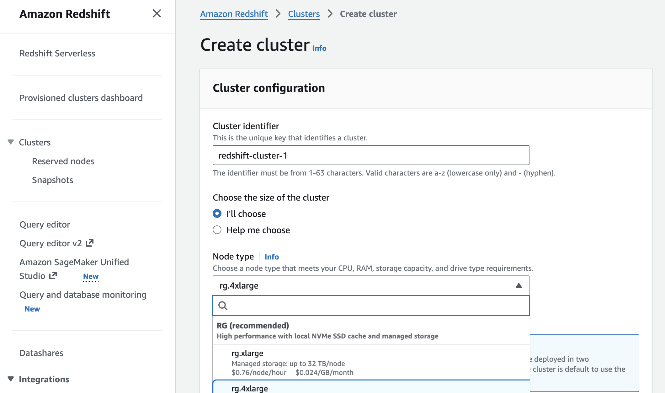
In the Amazon Redshift console, you can choose new RG instances when you create a cluster.
You can migrate previous-generation instances to RG instances with optimal paths based on your cluster configuration to estimate costs, validate compatibility, and automate execution.
Elastic Resize—in-place migration with 10-15 minutes downtime for compatible configurations
Snapshot and Restore—create a RG cluster from an RA3 snapshot. This is best for customers who want to make configuration changes during the migration
Your external tables, schemas, and query syntax—including existing Spectrum queries—remain unchanged. There is no need to recreate external tables or modify application code. To learn more, visit the Redshift Management Guide.
Amazon Redshift now executes data lake queries on cluster nodes—the same compute that processes data warehouse workloads. As a result, Amazon Redshift Spectrum is no longer required. Data lake queries stay within your VPC boundary, use existing IAM roles, and incur zero per-terabyte scanning charges. This removes the $5/TB Spectrum scanning fees that previously added to total Redshift costs.
Now available Amazon Redshift RG instances are now available in the following AWS Regions: US East (N. Virginia, Ohio), US West (N. California, Oregon), Asia Pacific (Hong Kong, Hyderabad, Jakarta, Malaysia, Melbourne, Mumbai, Osaka, Seoul, Singapore, Sydney, Taiwan, Tokyo), Canada (Central), Europe (Frankfurt, Ireland, Milan, London, Paris, Spain, Stockholm), Middle East (UAE), and South America (São Paulo). For Regional availability and a future roadmap, visit the AWS Capabilities by Region. For Redshift Provisioned, you can select On-Demand Instances with hourly billing and no commitments or choose Reserved Instances for cost savings. To learn more, visit the Amazon Redshift Pricing page.
As organizations scale their data processing and analytics workloads on Amazon EMR on EC2, observability across cluster health, job execution, and resource usage becomes increasingly important. Teams often manage log collection across distributed nodes, correlate Amazon EMR steps with underlying YARN applications, and configure monitoring agents to capture the right level of detail for their environment.
With Amazon EMR release 7.11.0 and updates to the Amazon EMR console, Amazon EMR on EC2 introduces observability capabilities that streamline these workflows further. In this post, we walk you through five key enhancements: Amazon CloudWatch Logs integration, step-level Amazon Simple Storage Service (Amazon S3) logging controls, expanded console UIs for YARN and Tez, Amazon EMR step to YARN application ID mapping, and enhanced custom metrics with updated documentation.
What’s new
The following sections cover key improvements across the Amazon EMR console, logging, metrics collection, and documentation to give you deeper, end-to-end visibility into your Amazon EMR clusters and workloads.
1. CloudWatch Logs integration
Starting with Amazon EMR release 7.11.0, you can stream cluster logs to Amazon CloudWatch Logs in near real time without requiring custom bootstrap actions or manual agent configuration. With Amazon CloudWatch logging enabled, Amazon EMR automatically captures and streams Amazon EMR step execution logs, Spark driver, and Spark executor logs as they’re generated. This makes them immediately available for monitoring, troubleshooting, and post-mortem analysis through the CloudWatch console or API.
You can enable CloudWatch logging through the Amazon EMR console during cluster creation or programmatically using the AWS Command Line Interfaced (AWS CLI) and SDK by including the Amazon CloudWatch Agent in your application configuration and specifying your logging preferences in the configuration section.
With minimal configuration, Amazon EMR captures step logs and Spark driver logs by default, streaming them to a log group named /aws/emr/{cluster_id}. For production workloads requiring stricter organizational and security controls, you can customize the log group name, define a log stream prefix for streamlined filtering, enable encryption with an AWS Key Management Service (AWS KMS) key, and explicitly select which log types to capture. The following example demonstrates a fully customized configuration:
This configuration directs the logs to a custom log group (/my-company/emr/production), prefixes log stream names with cluster-prod for consistent identification across clusters, encrypts log data at rest using the specified KMS key, and captures the full set of available log types: step stdout/stderr, Spark driver, and Spark executor output. Because logs are streamed to CloudWatch as they’re written, you have near real-time visibility into job execution without waiting for log aggregation to S3 or establishing direct connectivity to cluster nodes. Combined with CloudWatch Logs Insights, you can run structured querying across log streams, making it straightforward to trace failures, correlate errors across driver and executor logs, and build metric filters or alarms based on specific log patterns.
2. Step-level S3 logging improvements
S3 logging capabilities now provide granular control over how step logs are organized and secured. You can now specify a dedicated S3 log destination and AWS KMS encryption key at the individual Amazon EMR step level. This allows different steps within the same cluster to write logs to separate S3 paths with independent encryption configurations. This is particularly useful for multi-tenant clusters or workflows with varying data classification requirements.
Step-level logging is configured through the StepMonitoringConfiguration parameter, which accepts an S3MonitoringConfiguration object where you can define the target S3 path and an AWS KMS key for encryption at rest:
3. Enhanced console with direct access to monitoring UIs
Additional live application UIs are accessible directly from the Amazon EMR Console. These console-hosted interfaces remove the need to configure SSH (Secure Shell) tunnels, set up proxies, or establish any direct network connectivity to cluster nodes to reach application web UIs. The newly added interfaces include:
YARN ResourceManager UI – Monitor cluster-wide resource allocation, queue usage, and application lifecycle states across running and completed YARN applications. This interface also provides direct access to container-level logs for running YARN applications, enabling real-time debugging without requiring node-level access.
Tez UI – Inspect Hive query execution plans, DAG visualizations, vertex-level performance metrics, and task-level counters for queries executed through the Tez execution engine (for example, Hive and Pig workloads).
These join the existing Spark History Server and YARN timeline interfaces already available through the console. By surfacing these UIs, administrators can grant developers and analysts visibility into cluster workloads and application diagnostics without exposing direct network access to cluster infrastructure while maintaining tighter security boundaries and preserving full observability into job execution and resource consumption.
With these additions, Amazon EMR now offers three complementary approaches to accessing application web interfaces, each suited to different operational requirements. Live Application UIs provide console-hosted access to web interfaces on running clusters. They’re recommended for environments where direct network connectivity to cluster nodes must be restricted from end users. On-Cluster Web UIs offer full, unrestricted access to the complete set of native application web interfaces running on cluster nodes, suited for administrators and engineers who require deep, low-level visibility. Persistent Web UIs retain application-level data beyond cluster lifetime, so you can analyze and troubleshoot workloads on terminated clusters. Together, these options give you the flexibility to balance security boundaries, access scope, and data retention based on your team’s specific monitoring and debugging workflows.
4. EMR step to YARN application ID mapping
The Amazon EMR console now surfaces the YARN Application ID directly within the EMR step details panel. For each step executing a Spark, Hive, or other YARN-based workload, the console displays the submitted YARN Application ID associated with that step, establishing a direct link between the EMR step abstraction and the underlying YARN application. With this mapping, you can:
Directly correlate EMR steps to YARN applications – when a step fails or exhibits unexpected behavior, you can immediately identify the exact YARN application to investigate rather than manually cross-referencing timestamps or job names across interfaces.
Access live monitoring tools – with the YARN application ID readily available, you can navigate directly to the YARN ResourceManager Live UI or the Spark History Server to inspect resource consumption, task-level execution details, and application state for both running and completed jobs.
Retrieve logs for detailed troubleshooting – the application ID serves as the key lookup for retrieving container-level logs persisted to Amazon S3, significantly reducing the time to root-cause failures or diagnose performance regressions.
To use this feature, open the Steps tab on your Amazon EMR cluster detail page and select the step that you want to investigate. The YARN Application ID appears in the step details panel. From there, you can use the ID to navigate to the YARN ResourceManager Live UI at http://resourcemanager-host:8088/cluster/app/<application_id>, open the corresponding view in the Spark History Server, or locate the associated container logs in your configured S3 log destination.
5. Enhanced custom metrics and observability documentation
By default, Amazon EMR automatically sends cluster-level metrics to Amazon CloudWatch at five-minute intervals, covering YARN application states, node health, HDFS utilization, and I/O activity. With Amazon EMR Release 7.0 and later, enabling the Amazon CloudWatch Agent extends this baseline with additional detailed metrics collected at one-minute intervals across cluster nodes. Furthermore, Amazon EMR 7.1 introduced custom metric classifications that you can use to define precisely which component-level metrics to collect from Hadoop, YARN, and HBase subsystems, like DataNode I/O activity, NodeManager JVM heap utilization, container resource consumption, and HBase performance counters. Each classification supports configurable export intervals, giving you control over collection granularity based on your monitoring requirements.
After enabled, custom metrics are accessible directly from the Monitoring tab in the Amazon EMR console, where you can use a classification filter to switch between HDFS, YARN, HBase custom metric groupings that you’ve defined. Metric configurations can also be updated on running clusters through the console’s reconfiguration workflow, so you can adapt your monitoring strategy as workload requirements evolve without cluster downtime. For environments using Prometheus, metrics can also be forwarded to Amazon Managed Service for Prometheus and visualized through Grafana dashboards.
The following documentation and tutorials are available to help you get the most out of these capabilities:
Enhanced Custom Metrics Guide provides step-by-step instructions for configuring CloudWatch Agent to publish custom metrics.
EMR Observability Best Practices provides a comprehensive guide covering monitoring strategies, metric selection, and troubleshooting workflows.
Service Status Monitoring provides a tutorial on monitoring and publishing Amazon EMR application status.
These observability improvements are available now for Amazon EMR on EC2. To get started:
CloudWatch Logs integration and step-level log configuration: To use these capabilities, launch a new cluster with Amazon EMR release 7.11.0 or later.
For console enhancements: Navigate to your existing Amazon EMR clusters in the AWS Console to access Live Application UI links and YARN Application ID mappings in step details, with no additional configuration required.
For custom metrics: Review our Enhanced Custom Metrics documentation to configure the CloudWatch Agent for publishing Hadoop, YARN, and HBase component metrics using custom classification files.
Conclusion
With these enhancements, Amazon EMR on EC2 provides deeper visibility into cluster health, job execution, and resource usage, helping you reduce time to root cause and focus on delivering value from your data. Note that enabling CloudWatch Logs integration and custom metrics incurs additional CloudWatch charges based on log ingestion volume and metric publishing frequency.
If you have feedback or questions, reach out to your AWS account team or post on the AWS re:Post.
HBase operations teams spend hours manually correlating logs, metadata, and consistency reports to identify root causes. Traditional approaches require deep expertise and extensive investigation across scattered data sources, directly impacting MTTR and operational efficiency. As HBase deployments scale and expertise becomes increasingly scarce, organizations face mounting pressure to maintain service reliability while managing growing operational complexity. The manual nature of troubleshooting creates bottlenecks that delay incident resolution, increase operational costs, and risk service degradation during critical business periods.
In this post, we show you how to build an AI-powered troubleshooting solution using Amazon OpenSearch Service vector search and intelligent analysis. This solution reduces HBase inconsistency resolution from hours to minutes and root cause identification from days to hours through natural language queries over operational data. This democratizes HBase troubleshooting capabilities across teams and reducing dependency on specialized expertise.
Solution overview
The solution addresses HBase troubleshooting challenges through data processing, vector search, and AI-powered analysis. It processes operational data from Amazon EMR clusters, generates semantic vector embeddings, and enables natural language queries for intelligent troubleshooting. Key components include:
Amazon EMR HBase: Runs HBase workloads with Amazon S3 as the HBase rootdir for durable, scalable storage
Data Processing: Extracts and processes HBase logs, HBCK reports, and metadata with vector embeddings
Amazon OpenSearch Service: Provides vector search capabilities with k-NN algorithms for semantic analysis
AI Analysis Interface: Enables natural language queries with context-aware recommendations
Custom Knowledge Base: Supports organization-specific runbooks and troubleshooting procedures by ingesting Git repositories via Kiro CLI‘s /knowledge add command, enabling the AI assistant to reference custom operational guides alongside HBase source code and operational tools
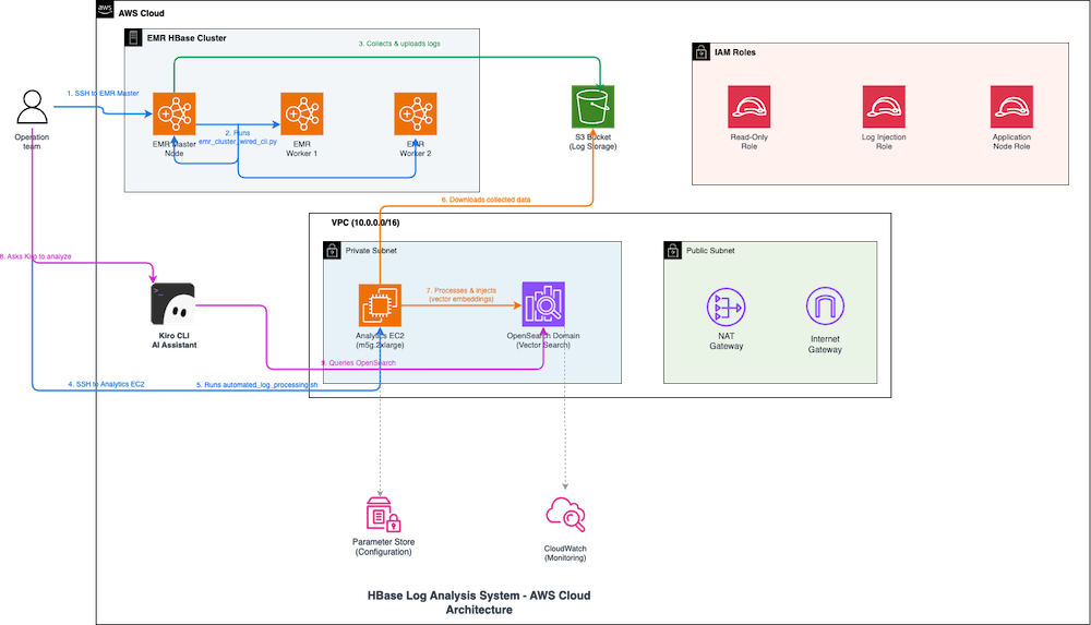
The preceding diagram illustrates how the HBase log analysis system troubleshoots inconsistencies through automated workflows across AWS services.
When an operations team needs to investigate HBase issues, the engineer connects over SSH to the Amazon EMR primary node and runs the error collection script, which gathers logs from HBase master and RegionServer nodes and uploads them to Amazon S3. Next, the engineer connects to the Analytics Amazon Elastic Compute Cloud (Amazon EC2) instance and executes the automated processing script, which downloads logs from Amazon S3, generates semantic vector embeddings, and injects them into Amazon OpenSearch Service for k-NN-based semantic search. The engineer then queries the Kiro CLI AI Assistant using natural language to investigate. Kiro searches Amazon OpenSearch Service for relevant log entries and uses Amazon Bedrock to analyze patterns, correlate errors across components, and provide actionable recommendations. This reduces troubleshooting time from hours to minutes. The system operates within an Amazon Virtual Private Cloud (Amazon VPC) with private subnets for Amazon EMR and Analytics Amazon EC2, AWS Identity and Access Management (AWS IAM) roles for access control, Parameter Store for configuration, and Amazon CloudWatch for monitoring.
Prerequisites
For this walkthrough, you need the following prerequisites:
AWS account setup
An AWS account with administrative access for initial deployment
AWS Command Line Interface (AWS CLI) configured with administrative credentials
Required AWS IAM permissions
For infrastructure deployment
Your deployment user or role needs the following permissions:
The user or role must have the ability to create AWS CloudFormation stacks.
Infrastructure deployment:
For infrastructure deployment, you need AWS CloudFormation stack management permissions.
You also require sufficient access to create and manage the following resources:
Amazon OpenSearch Service domains
Amazon EC2 instances, Amazon VPCs, security groups, and networking components
AWS IAM roles and policies
AWS Systems Manager Parameter Store entries
Amazon CloudWatch Logs groups
Amazon S3 bucket for access logs and session logs
Runtime service roles
The AWS CloudFormation stack automatically creates two specialized AWS IAM roles designed with least-privilege access principles.
The first role is the Amazon OpenSearch Service Role, which manages Amazon VPC networking and Amazon CloudWatch logging for the Amazon OpenSearch Service domain.
The second role is the Application Role, which provides minimal Amazon OpenSearch Service and Amazon S3 access specifically for log processing applications and secure log ingestion operations.
Network requirements
Amazon VPC with private subnets for secure Amazon OpenSearch Service deployment
NAT Gateway for outbound internet access from private subnets
Security groups configured for HTTPS-only communication
Running Kiro CLI on Amazon EC2
Kiro platform requirements:
Kiro subscription
Active Kiro License: Valid subscription to Kiro platform
User Account: Registered Kiro user account with appropriate permissions
API Access: Kiro API keys or authentication tokens for CLI access
Permission Sets: Configured permission sets for Kiro users with appropriate AWS access
User Assignment: Users assigned to relevant AWS accounts and permission sets
SAML/OIDC Configuration: Identity provider integration if using external identity systems
Additional prerequisites
Python 3.7+ and Node.js installed locally
Python 3.11+ for AWS Lambda runtime environment (required for OpenSearch MCP server compatibility)
Sufficient service quotas for Amazon OpenSearch Service instances and Amazon EC2 resources
Recommended access to the analysis instance via AWS Systems Manager Session Manager (recommended). Amazon EMR clusters running HBase workloads
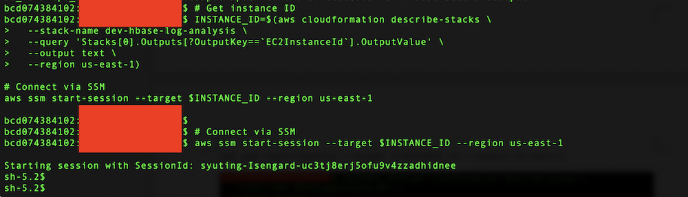
EMR_EC2_Default_Role of Amazon EMR EC2 instance profile can execute describe-stacks on AWS CloudFormation stacks in us-east-1
Basic familiarity with HBase operations
The deployment follows AWS security best practices with resource-specific permissions, regional restrictions, and encrypted data storage. All AWS IAM policies implement least-privilege access patterns to help secure operation of the log analysis pipeline.
Walkthrough
This walkthrough demonstrates deploying and configuring the AI-powered HBase troubleshooting solution in five key steps:
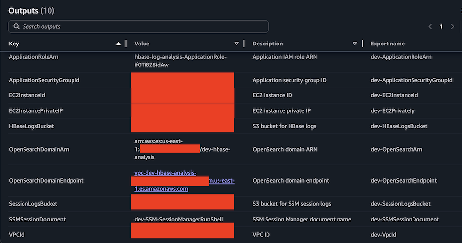
Deploy AWS infrastructure using AWS CloudFormation
Kiro CLI and configuration with AWS IAM Identity Center authentication. The script will automatically add Apache HBase open source repo and Apache HBase open source operational tools to knowledge bases
HBase source repositories for your Amazon EMR version
Python dependencies and MCP server configuration
Add your own knowledge base to Kiro CLI
To enhance Kiro CLI’s analysis capabilities with Apache HBase open-source repositories, your organization’s HBase runbooks and troubleshooting guides, you can add your own knowledge base repositories. Here are the commands. Please periodically validate and maintain your runbook contents so that they remain accurate and up-to-date, reflecting any changes in your HBase environment, configurations, or operational procedures.:
Set up data collection from your Amazon EMR clusters to gather HBase logs, metadata, and consistency reports using the recommended direct collection method. To configure Amazon EMR log analysis collection
On your Amazon EMR cluster primary node, run the following commands to download the collection scripts:
# On EMR primary node
sudo su - hadoop

# Fork and clone the source code repository on GitHub: sample-emr-hbase-inconsistencies-detection-recovery-mcp-kiro
git clone https://github.com/YOUR_USERNAME/sample-emr-hbase-inconsistencies-detection-recovery-mcp-kiro.git hbase-analysis
cd hbase-analysis
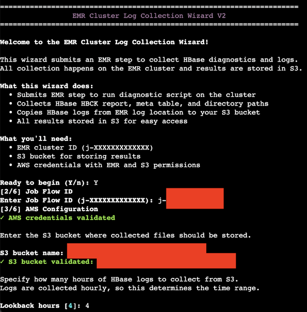
Run the interactive collection wizard:
# Run collection wizard
python3 scripts/utilities/emr_log_collection/emr_cluster_wizard_v2.py
Input the parameters like the EMR cluster’s jobflow ID, the log analysis Amazon S3 bucket name, and the lookback hours. The default value of the lookback hours is 4 hours.
The collection wizard performs these actions:
Collects HBase logs from local filesystem. Please reference to prerequisites for the access permission.
Runs hdfs dfs -ls -R /hbase or aws s3 ls <hbase-root-dir> –recursive
Runs hbase shell <<< 'scan "hbase:meta"'
Creates properly named files matching analysis system requirements
Uploads to Amazon S3 with correct naming conventions
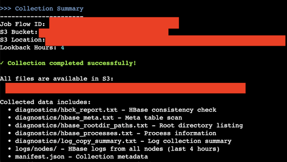
Here’s the data collection summary:
You can check the uploaded contents through AWS CLI.
aws s3 ls s3://<log-path> --recursive
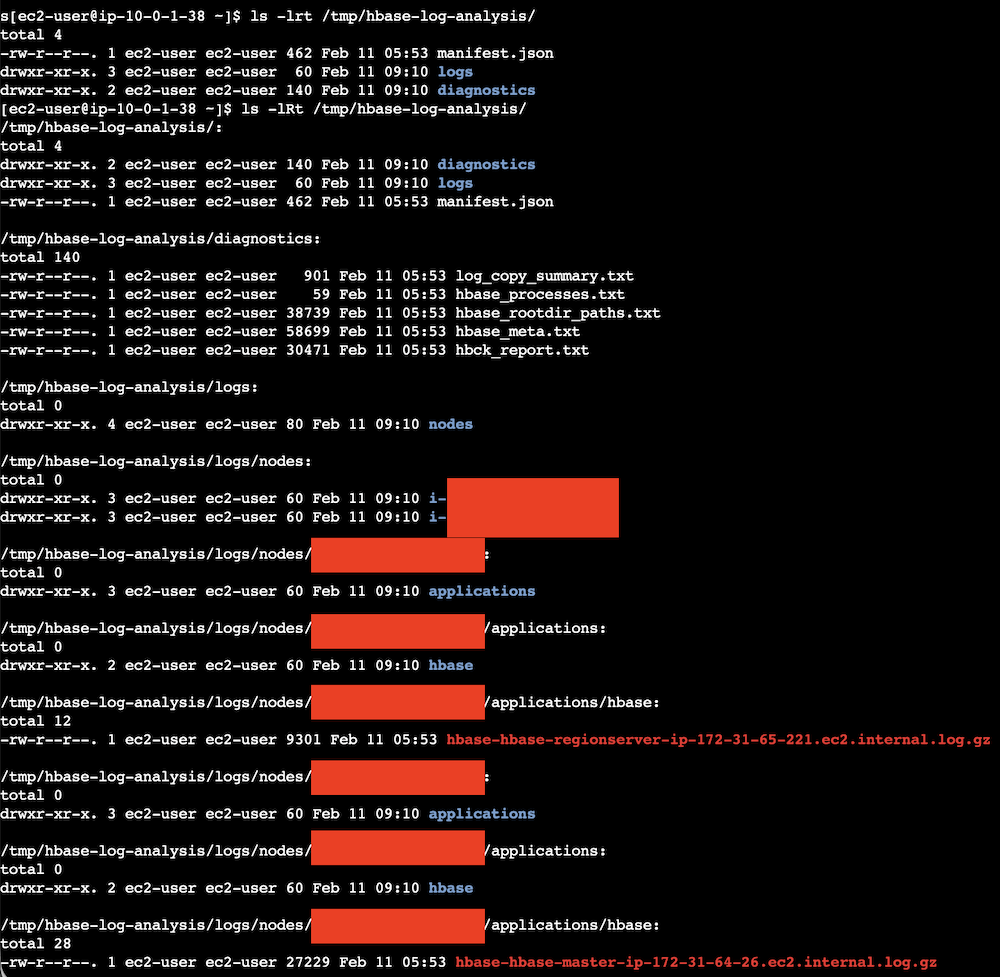
Here’s a screenshot of the outputs.
On the Analysis Amazon EC2 instance, download collected files to the Analysis Amazon EC2 instance.
# On analytics EC2 instance
sudo su - ec2-user

# Download logs from S3
mkdir -p /tmp/hbase-log-analysis
cd /tmp/hbase-log-analysis
aws s3 sync s3://<S3-BUCKET-NAME>/emr-logs/<EMR-JOBFLOW-ID>/ .
You can get your jobflow ID from Amazon EMR console:
The generated files (hbase-hbase-master-ip-xxx-xxx-xxx-xxx.ec2.internal.log.gz, hbase-hbase-regionserver-ip-xxx-xxx-xxx-xxx.ec2.internal.log.gz, hbck_report.txt, hbase_rootdir_paths.txt, hbase_meta.txt, hbase_processes.txt, log_copy_summary.txt) should be aligned with the automated processing script requirements as following.
Step 4: Process and index data
Process the collected HBase data and create vector embeddings for intelligent search capabilities.To process and index the data, please navigate to the project directory on the Analysis EC2 instance, and run automated-log-processing.sh:
sudo su – ec2-user
cd ~/hbase-analysis
chmod +x ./scripts/processing/automated-log-processing.sh
./scripts/processing/automated-log-processing.sh \
  --job-flow-id j-YOUR-JOB-FLOW-ID \
  --stack-name dev-hbase-log-analysis
The processing scripts extract and parse HBase logs and generate dimensional vector embeddings from HBase log messages using sentence transformer models to enable semantic search beyond keyword matching. The system uses the all-MiniLM-L6-v2 model by default (producing 384-dimensional embeddings), but supports configurable models with different embedding dimensions, automatically adapting the OpenSearch vector index to match the chosen model’s output. The system processes comprehensive HBase operational data including region operations, compaction activities, Write-Ahead Log events, memstore operations, and cluster management information from HMaster and RegionServer logs. Vector embeddings capture error messages, exception stack traces, performance warnings, and multi-line log entries through intelligent text preprocessing. This semantic representation enables advanced troubleshooting where users can query conceptually for “region server performance issues” or “memory pressure” and receive contextually relevant results across different log files and time periods. The vector search capabilities support error correlation by grouping similar exceptions, performance analysis by identifying related bottlenecks, and operational pattern recognition. Each log entry is stored in Amazon OpenSearch Service with original metadata (timestamp, log level, source file, job flow ID) alongside the embedding vector, enabling both structured queries and AI-powered semantic analysis. This approach transforms raw HBase logs into a searchable knowledge base supporting anomaly detection, trend analysis, and predictive insights for proactive cluster management and troubleshooting.
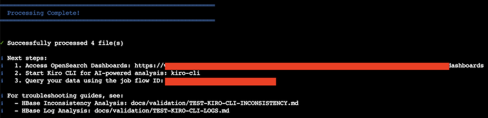
All scripts use AWS IAM authentication automatically. Here’s a screenshot of the data processing outputs.
Step 5: Enable AI-powered analysis
Configure the AI analysis interface to enable natural language queries against your HBase operational data.
To set up AI-powered analysis
Launch Kiro CLI (already configured by automated setup):
kiro-cliCheck mcp and knowledge bases. /mcp list
/knowledge show
If you cannot see these 2 knowledge bases, you can manually add them through the following commands:
# Note: Large repositories (~500MB) may take a while to index. Check progress with: /knowledge show
/knowledge add --name "HBase operational tools" --path /opt/hbase-repositories/hbase-operator-tools"
/knowledge add --name "Apache HBase source code" --path /opt/hbase-repositories/hbase"
Use natural language queries to analyze your HBase data. The AI analysis uses both the OpenSearch MCP Server for querying indexed data and the Filesystem knowledge bases for accessing HBase source code. You can add your custom runbooks for Kiro’s reference as well.
For HBase inconsistency analysis:
# HBase Inconsistency Detection and Remediation Guidelines
## Search Strategy
- Use fuzzy search for case variations/typos, term query for exact region IDs, match_phrase for paths, query_string for logs
- Always use .keyword subfields for exact text matching
- Cross-reference filesystem (wildcard: {"wildcard": {"path": "*<region_id>*"}}) with hbase:meta (match: {"match": {"row_key": "<region_id>"}})
- The total region count in hbase meta must match the total matched document count of wildcard path like "*/.regioninfo" in hbase rootdir path.
- All terms of region_name.keyword for a region encoded name must match a wildcard path like "*/.regioninfo"
- All terms of table_name.keyword for a table must match a wildcard path like "*/.tabledesc*"
- 1595e783b53d99cd5eef43b6debb2682 is the master store region that will locate in <hbase-root-dir>/MasterData/data/master/store/1595e783b53d99cd5eef43b6debb2682/
- May cross check with the raw logs in /tmp/hbase-log-analysis/
## Issue Types
Orphan regions, missing .regioninfo, missing/extra regions in hbase:meta, rowkey holes, stuck RIT, master initialization failures
## Analysis Steps
### 1. Cross-Reference Meta vs Filesystem
- Filesystem regions NOT in hbase:meta → ORPHAN REGION
- Meta regions NOT in filesystem → MISSING REGION
### 2. Validate Region Chain Continuity
- Sort regions by STARTKEY, verify region[i].ENDKEY == region[i+1].STARTKEY
- First STARTKEY must be '', last ENDKEY must be ''
- Gaps → ROWKEY HOLE
### 3. Check Region States
- state != 'OPEN' → Check RIT
- Missing server assignment → UNASSIGNED
- Multiple servers → SPLIT BRAIN
- "deployed_servers" field must have only one region server address like "ip-xxx-xxx-xxx-xxx.ec2.internal,16020,1770781485397" . The value should not be null or have multiple values.
### 4. Validate .regioninfo Files
- Missing .regioninfo in region directory → CORRUPT REGION
### 5. Cross-Check HBCK Report
- Compare orphan counts, RIT regions, filesystem vs meta region counts
### 6. Analyze Logs
- Search: "updating hbase:meta row=<region>", "STUCK", "RIT", "Failed" + "<region>", "Split"/"Merge" + "<region>"
## Remediation
- Reference knowledge bases: "Apache HBase source code", "HBase operational tools"
- Use hbck2: /usr/lib/hbase-operator-tools/hbase-hbck2.jar
- Prefix commands with sudo -u hbase
- Use aws s3 for S3-based rootdir
- Wait 300s after creating holes before hbck fixMeta (catalog janitor cycle)
- Use unassign instead of deprecated close_region
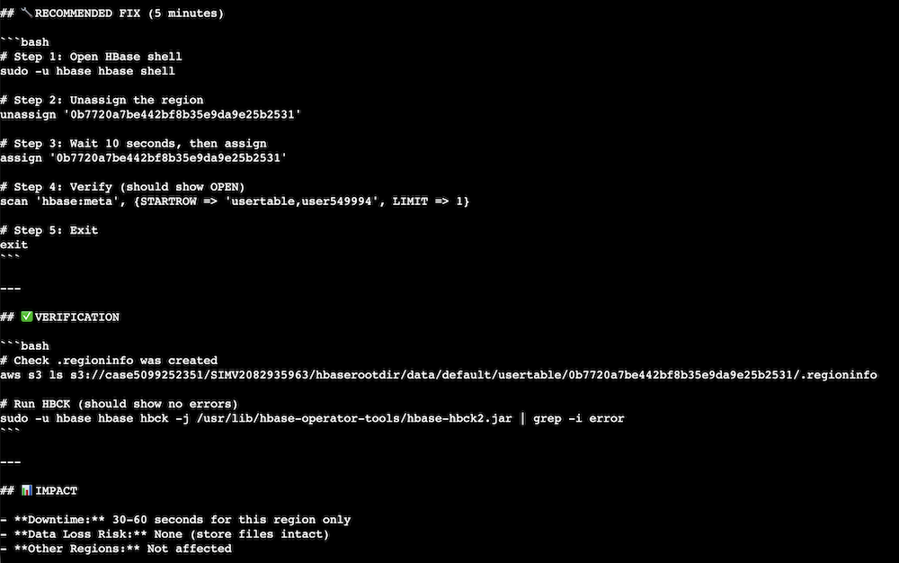
- If the region does not have .regioninfo in  <hbase-root-dir>/data/<namespace>/<table-name>/<region-encoded-name>/ but hbase:meta has that region's information and that region has been deployed on a healthy region server, you can use hbase shell to unassign and assign the region to re-generate .regioninfo
- Always add "sudo -u hbase hbase" before "hbase shell" and "hbase hbck" commands
## Job flow
Target: <your-job-flow-id>
Inconsistency to detect: All kinds of inconsistencies
You can trust or input “y” or “t” to grant Kiro to search through mcp and knowledge bases.
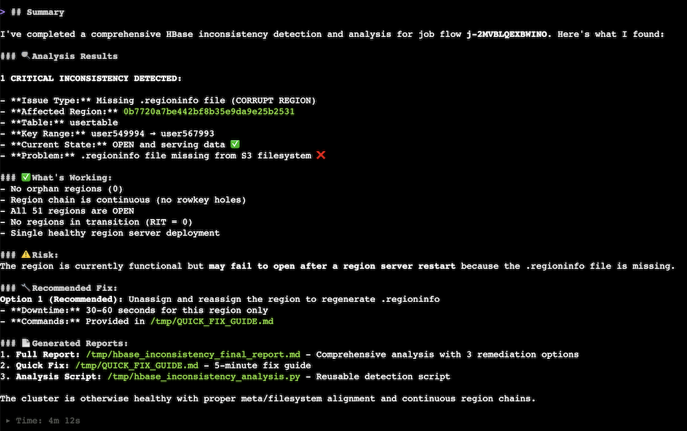
You may get some outputs like this: Kiro checked for any HBase issue.
Kiro summarized the examination results.
Kiro provided mitigation commands after Kiro summarized the issue.
Cleaning up
To avoid incurring future charges, delete the resources created during this walkthrough.
In this post, we showed you how to build an AI-powered HBase troubleshooting solution that transforms manual log analysis into an automated workflow. By combining Amazon OpenSearch Service vector search with Amazon Bedrock-powered analysis through the Kiro CLI, operations teams can resolve complex HBase inconsistencies faster and gain deeper operational insights. The solution demonstrates how AI augments human expertise to improve operational efficiency, reducing HBase inconsistency resolution from hours to minutes and root cause identification from days to hours. Ready to transform your HBase operations? Get started with the GitHub repository and explore the Amazon OpenSearch Service documentation for additional guidance on vector search capabilities.
Acknowledgments
The author would like to thank Xi Yang, Anirudh Chawla, and Sasidhar Puthambakkam for their contributions to developing the technical solution. Xi Yang is a Senior Hadoop System Engineer and Amazon EMR subject matter expert at AWS. Anirudh Chawla is an AWS Analytics Specialist Solution Architect who helps organizations empower businesses to harness their data effectively through AWS’s analytics platform. Sasidhar Puthambakkam is a Senior Hadoop Systems Engineer and Amazon EMR Subject Matter Expert who provides architectural guidance for complex BigData workloads.
Cloud and AI are transforming industries and societies at unprecedented speed, from accelerating research and enhancing customer experiences to optimizing business processes and enriching public services. At Amazon Web Services (AWS), we believe that for the cloud and AI to reach their full potential, customers need control over their data and choices for how and where they run their workloads. In 2022, we formalized our commitment to control and choice—offering all AWS customers the most advanced set of sovereignty controls and features available in the cloud with the AWS Digital Sovereignty Pledge. As AI adoption accelerated, we’ve been working with customers to help them embrace AI innovation while meeting sovereignty requirements. We’re committed to ensuring customers can continue to harness AI’s transformative capabilities without compromising on the capabilities, performance, innovation, security, and scale of the AWS Cloud to meet their sovereignty needs, including AI sovereignty. Our approach to AI sovereignty is grounded in a deep understanding of these needs and the real-world implementation challenges that come with them.
Through discussions with customers, partners, analysts, and regulators, we’ve learned that digital sovereignty—and AI sovereignty—means different things to different stakeholders. Each country and region has unique, evolving sovereignty requirements, with no uniform guidance on which workloads or sectors must comply. Despite this variation, we’ve identified consistent themes: data sovereignty (including data residency and operator access restrictions) and operational sovereignty (including resilience, survivability, and independence). AI sovereignty builds on these foundations, adding emerging considerations such as preserving cultural norms, values, and local languages in AI outputs. Ultimately, meeting digital and AI sovereignty requirements comes down to providing customers with more control and choice.
Enabling customer control and choice across the AI stack
AI sovereignty requires control and choice across the AI stack—comprehensive cloud infrastructure that combines compute, networking, data management, security controls, specialized application services, and talent. This includes the ability to make deliberate choices across the stack such as location, dependencies, services, and partners that align with customers’ unique needs, regulatory requirements, and innovation objectives. With AWS, customers can develop AI on a trusted foundation where their data remains secure and under their control. Customers have the freedom to choose from a comprehensive range of AI optimized chips—including purpose-built AWS silicon and chips from NVIDIA, AMD, and Intel—so they can select the right chip for the right workload. AWS applies two decades of learned expertise to our comprehensive AI stack, enabling organizations to maintain complete control over their data and operations while accessing cutting-edge capabilities to solve local challenges.
AWS provides customers with the infrastructure and tools to embed AI across the full value chain—not just in isolated use cases, but as a foundational capability enabling them to train and deploy models and build sophisticated AI and generative AI applications with exceptional performance. This enables customers to focus on innovation instead of their infrastructure, bringing the cloud to where they need it most with a range of options including AWS AI Factories, AWS Outposts, AWS Local Zones, AWS Dedicated Local Zones, and AWS Regions including the AWS European Sovereign Cloud. For example, customers who require dedicated deployments to meet their sovereignty requirements for their mission-critical AI workloads can use AWS AI Factories. These physically isolated, dedicated deployments built exclusively for the customer combine the latest AI infrastructure, including AWS Trainium accelerators, NVIDIA GPUs, dedicated networking, and storage. AWS AI Factories address AI sovereignty needs by delivering on-premises AI capabilities to securely perform training, fine tuning and real-time inference.
The AWS AI portfolio offers a comprehensive range of services—from foundation models (FMs) through Amazon Bedrock, to machine learning offerings like Amazon SageMaker, application services like Amazon Q, and developer tools like Kiro—designed to give customers control over their data and choice in how they deploy AI. With Amazon Bedrock, customers can choose from hundreds of models from leading providers like AI21 Labs, Anthropic, Amazon, Cohere, Mistral AI, and OpenAI. Customers can evaluate and select the most suitable FMs for their specific needs and choose where they deploy them, and fine-tune models privately with their own data. Customers are always in control of their data. Critically, no customer inputs to or outputs from Amazon Bedrock are used to train Amazon Nova or any third-party models.
Supporting national AI strategies
Successful AI strategies require building a holistic environment nurturing local talent, supporting startups, developing industry-specific applications, and fostering public-private partnerships. The cloud has transformed AI from an exclusive technology requiring massive investment into an accessible tool for innovation across all sectors and organization sizes. While technical infrastructure gets much of the attention when considering AI sovereignty, the cultural and strategic dimensions of national FMs are equally critical. These FMs aren’t merely computational tools, they can encode elements of cultural knowledge, linguistic nuance, and societal context, making local relevance a design consideration rather than an afterthought. These FMs serve purposes that extend beyond technical capabilities. Locally trained FMs can reflect national educational curricula and cultural values while understanding local legal systems, business practices, and regulatory frameworks. Models trained on local languages, dialects, and cultural contexts support linguistic diversity and help underrepresented languages gain representation in AI products and services.
AWS supports vital national priorities and customers’ missions, such as the preservation of culture norms, values, and local languages development of regional and local language model capabilities. To customize models, customers can use Amazon SageMaker AI for voice, domain specialization, and to evaluate models for accuracy. For example, the first Greek LLM made available in March 2024 was Meltemi—built on top of Mistral-7B, running on AWS infrastructure, and continually pretrained to extend its proficiency in the Greek language using a dataset of 28.5 billion Greek tokens. Meltemi is available on HuggingFace. SEA-LION—a family of open source, multilingual LLMs for Southeast Asia—was trained entirely on AWS with managed GPU clusters. Their team completed a 3B-parameter model in only 3 months—a 60% faster timeline than comparable on-premises projects.
Verifiable control over data access
Sovereignty isn’t only about where data resides—it’s about who can access it and under what conditions. In the AI context, access restriction extends beyond infrastructure to cover model inputs, outputs, training processes, and the operational environments in which AI runs. Unlike traditional infrastructure, AI workloads introduce new access surfaces: the model itself, the data used to train it, and the inference pipeline through which sensitive inputs flow. This furthers the need for verifiable governance and identity propagation in IT systems.
To help ensure the confidentiality and integrity of customer data, all modern Amazon Elastic Compute Cloud (Amazon EC2) instances including those that offer AI accelerators, such as AWS Inferentia and AWS Trainium, are backed by the industry-leading security capabilities of the AWS Nitro System. By design, there is no mechanism for anyone at AWS to access customer data on Nitro EC2 instances that customers use to run their workloads. AWS services—including those with AI capabilities built on Amazon EC2—inherit these same protections. These protections apply to AI data running in the AWS Nitro System so that they’re protected at every stage—from model training to inference. The NCC Group, an independent cybersecurity firm, has validated the design of the Nitro System. We believe providing this level of transparency is critical in building and sustaining trust.
As AI agents increasingly take actions across systems on behalf of users, controlling who and what can access resources—and ensuring appropriate human oversight—becomes critical. AWS Identity and Access Management (IAM) helps ensure that only authorized users and applications can access AI resources through fine-grained permissions and comprehensive audit trails. For AI agents and automated workloads, Amazon Bedrock AgentCore Identity provides identity and credential management, so agents operate with the right permissions and nothing more.
Transparency and assurance
Transparency is at the core of our digital sovereignty commitment. We provide comprehensive industry-leading technical measures, operational controls, and contract protections that give customers control over where they locate their data, who can access it, and how it’s used. To give greater assurance on how AWS services are designed and operated, we continue to seek out and secure third-party attestations, accreditations, and certifications that help our customers meet their compliance needs.
We continue to deepen our assurances and transparency to customers—such as updating our AWS Service Terms to reflect our technical protections commitments (e.g. AWS Nitro System), providing detailed commitments as to our handling of thirid-party requests for customer data in our agreements, and providing supplemental explanations and resources (e.g. CLOUD Act blog) to empower customers to make informed choices on sovereignty matters. These efforts extend into our commitment to responsible AI, providing customers the confidence to build and operate AI applications responsibly using AWS Services. ISO/IEC 42001 is an international management system standard that outlines requirements and controls for organizations to promote the responsible development and use of AI systems. AWS is the first major cloud service provider to achieve ISO/IEC 42001 accredited certification for AI services, covering Amazon Bedrock, Amazon Q Business, Amazon Textract, and Amazon Transcribe. In November 2025, AWS successfully completed its first surveillance audit for ISO 42001:2023 with no findings, reiterating the continual commitment of AWS to responsible AI practices.
Innovative technology requires a secure and trustworthy foundation. AWS supports more than 140 security standards and compliance certifications that our customers and partners can inherit to help comply with local laws and regulations. For two decades, we’ve deeply engaged with regulators and cybersecurity authorities to align our offerings with national priorities and ensure our solutions support both innovation and control. We actively contribute to frameworks that respond to new developments without stifling progress.
Sustained commitment to helping customers achieve their sovereignty goals
AWS is committed to giving customers the same control and choice over their AI systems as they have over their data. We help customers harness AI’s transformative power while maintaining the capabilities, performance, innovation, security, and scale of AWS Cloud. As cloud and AI evolve, AWS will continue offering the most advanced sovereignty controls and features available.
If you have feedback about this post, submit comments in the Comments section below.
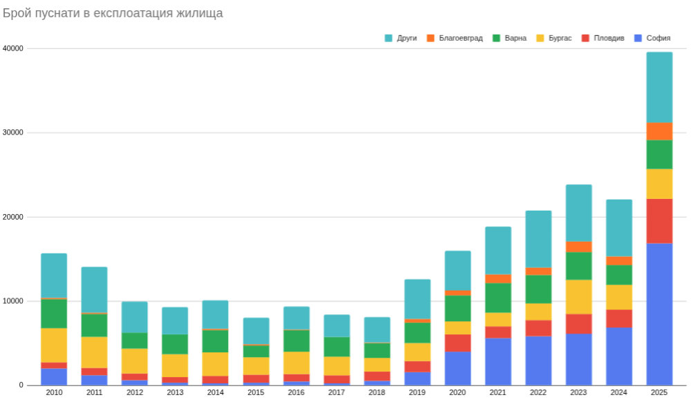
Ако ви се струва, че все повече сгради да никнат около вас, въобще не си въобразявате. Общо 39594 жилища са пуснати в експлоатация в България миналата година спрямо 22 хиляди през 2024-та. За това има исторически причини и доста детайли, които личат от данните на НСИ. Паралелно населението на страната е намаляло с над 22 хиляди души за тези две години.
В последните седмици бяха обновени доста показатели в статистиката. Тъй като има много начини да се съпоставят, разделих темата на няколко части. Първо, както винаги, описвам условностите в данните и какво няма да видим в тях. Второ показвам жилищата в строеж, с разрешение и пуснати в експлоатация за цялата страна, както и по брой стаи. След това разглеждам поотделно тези данни за областите София, Пловдив, Благоевград, Варна и Бургас. После сравнявам ключови параметри и аномалии между областите. Накрая правя съпоставям с демографските данни и динамиката на домакинствата.
Условности
НСИ събира информация за разрешенията за строеж, започнатите сгради и пуснатите в експлоатация от различни източници. Колкото и методологията да е описана ясно, има практически разминавания, с които всички ние сме наясно. Например, измерването на полезна и жилищна площ се разминава между инвеститори, както ясно се вижда от обявите и като гледате на място. Отделно има промяна на методологията и след 2018-та смятат в жилищната площ кухните над 4 кв.м.
Има доста сгради, които се използват и в тях живеят от години семейства, които не са пуснати в експлоатация. Отделно има немалко жилища, които са незаконно изградени и разширени. Има цели такива сгради и етажи. Те не влизат в тази статистика. Също така, във времето между разрешението и пускането в експлоатация сградите претърпяват промени – по-често съкращаване на паркоместа, но понякога и разделяне или сливане на жилища. Не на последно място, има доста сгради, които не се водят за жилищни, но всъщност са такива заради лобистки недъзи в ЗУТ и общите устройствени планове на големите ни градове. Това се вижда най-вече в данните за започнатите строежи.
Не на последно място, тук разглеждаме само жилищни сгради и жилищата в тях. В сградите им има офиси, студия и други, които бързо се обръщат в жилища, но официално не се водят за такива. Има го и обратното – жилища се превръщат в офиси. Има сгради, които се водят формално за хотели, но продават апартаментите в тях. Те отново не влизат в тази статистика. Доколкото повечето си представяме блокове и бетонни стени по булеварди, много от тези жилища са и къщи. Именно те заемат по-голямата част от сегмента с 4 и повече стаи.
Всичко това би могло да повлияе на данните подадени на НСИ. За съжаление, оказва се изключително трудно да научим колко сгради са на ниво акт 14, но не са пуснати в експлоатация. Това би ни дало представа за някои от тези недъзи. От години се опитвам да събера такава справка. Миналата седмица пуснат запитване до НАП, които би трябвало да имат такива данни, и се надявам да ми предоставят справка.
Разрешени, в строеж и готови
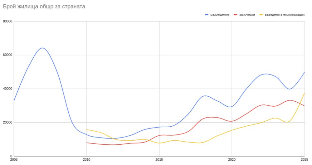
Информация за тези фази на строежите ни дава НСИ заедно с доста параметри по тях. Това ни позволява да разгледаме не само стряскащото число за миналата година, а как се развива през времето. Виждаме, че наистина почти 40 хиляди жилища са били пуснати в страната, но общо 225 хиляди са били разрешени за строеж в последните 5 години. За същия период 139 хиляди са започнали да се строят.
Всъщност, миналата година за пръв път от последните 20 броят на жилищата е надвишил броя на започнатите строежи. Това ни дава индикация, че има много незавършени такива, както и много, които се използват без акт 16. Има много обяснения защо именно през 2025-та има такъв голям натиск да се довършат и повечето не си противоречат. Няма да се впускам в тях сега.
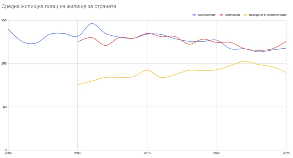
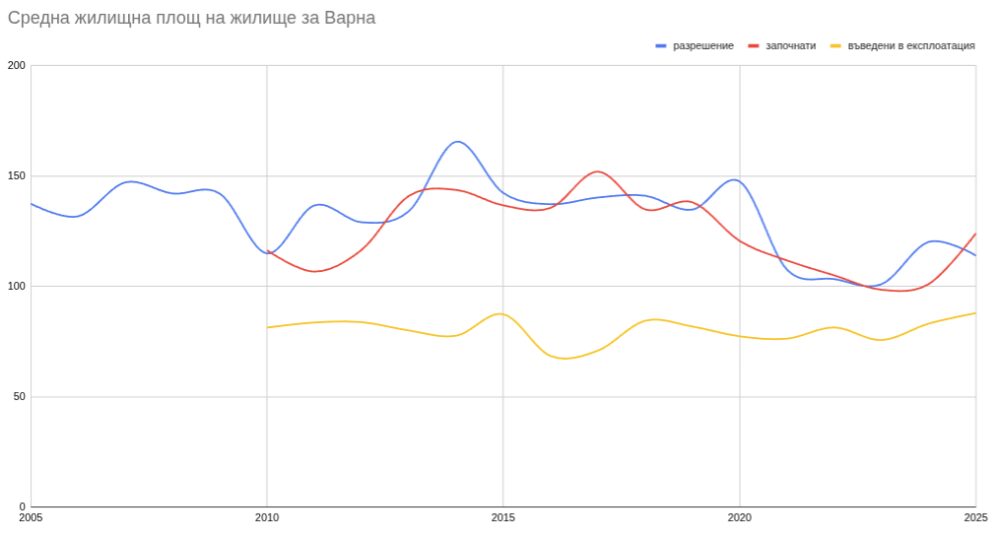
Интересно наблюдение има когато разделим полезната площ на броя жилища в данните на НСИ. Противно на пазарните анализатори, че се търсят по-големи жилища и пазара се ориентира към такива, всъщност има отчетливо намаление в разрешителните и започнатите строежи с около 10%. Това обаче са декларираните данни от строителите и те твърдят, че строят жилища средно по 115 до 130 кв.м. Това четем и по обявите и красивите обещания на зелено. Реално когато влязат в експлоатация и полезната площ пада на 90 до 100 кв.м. От нея жилищната площ, т.е. без идеални части, е между 65 и 80 кв.м. Забелязва се, че в последните 3 години жилищната площ на готовите жилища всъщност намалява с над 20%
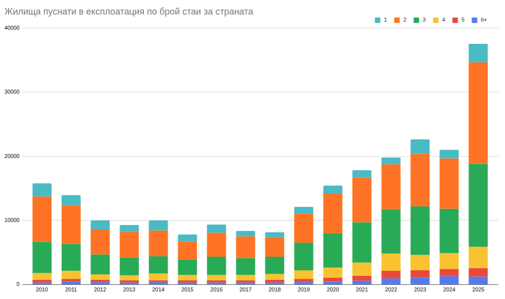
Погледнато по стаи виждаме, че има увеличение на жилищата с 6 и повече, но не много. Най-големият растеж е сред тези от 2 и 3 стаи. С изключение на 2024-та, има растеж и на едностайните. Това отново противоречи на тиражираните от представяни за експерти на имотния пазар, строители, анализатори и инфлуенсъри тези как се движи пазара и какво се търси най-много. Алтернативно обяснение, че инвеститорите просто не следват съветите на изброените и строят каквото им е удобно. Както вече писах, този пазар не е особено пазарен, особено що се отнася до определянето на цените.
Растежът през последната година обаче озадачава. Особено след спадът средно за странта през 2024-та. Това важи не само за София, но и за областите Пловдив, Бургас, Варна и … Благоевград. Броят жилища пуснати в експлоатация в София и Пловдив през 2025-та е бил два пъти и половина повече от предходната година. Във Варна – с 50% повече, а в Благоевград – 90% повече. В Бургас е около средното за страната – 21%, но там пикът беше 2023-та. 10 хиляди от това увеличение е само в София.
На следната графика се вижда по-ясно тази промяна. Растежа започва още 2019-та подхранван най-вече от строителството в София. Това не значи, че не са започнати строежи, за което ще стане дума по-късно, а че не са довършени и пуснати в експлоатация. Бургас, Варна и Пловдив са относително стабилни до 2022-ра. През 2024-та има привиден спад но той е заради намаление извън София.
Тази графика създава впечатлението, че в София и Пловдив бетонирането надлъж и нависоко преуспява. Гледайки готовите сгради това е така, но историите са доста различни. Затова е важно да вникнем в данните на отделните области, за да разберем какво се случва.
Тук е важно да се разбере, че разрешенията за строеж са често формалност. Понякога са на база дела където административните съдилища са отменили предходен отказ. По-често почвата е била утъпкана – в буквален и преносен смисъл – с промени на ПУП на парче, решения на общински съвети, спорни градоустройствени заповеди и едноименни поправки на закони в парламента. След това въпросът по принцип не е дали ще се застроява, а как и колко.
София
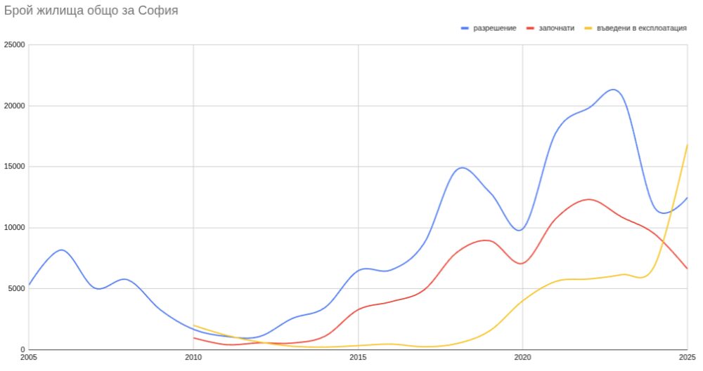
В София виждаме огромно увеличение на разрешенията за ползване. Една част са на малки сгради на общината, а големите сгради са от ДНСК. Справка в картата с документи от градоустройството на GovAlert показват 778 документа в тази категория от ДНСК и 1493 – от общината. Разбира се, не всички са жилищни сгради, каквито 2468 са пуснати в експлотация миналата година. Това значи, че за поне 200 нямаме публична информация, вероятно защото документите не съдържат достатъчно ясна идентификация на имота или просто не са публикувани.
Виждаме обсъждания вече скок на готовите жилища. Вижда се и пикът е разрешенията за строеж между 2020 и 2023. От 2024-та нататък разрешенията за строеж падат наполовина. Аналогичен е спада и на новозапочналите строежи на сгради. Това включва както големи кули , така и отделни къщи или комплекси от такива. Графиката долу, както и останалите подобни, не отчита броя разрешения за строеж, а жилищата упоменати в тях.
Това ни дава индикация, че довършените сгради в последната година са разрешени и започнати в последните години. Предвид натрупаните разрешения и множеството течащи строежи не очаквам да намалее потокът от готови жилища в близките години. Ако се запази обаче спада на започнатите такива, след няколко години ще има спад и там.
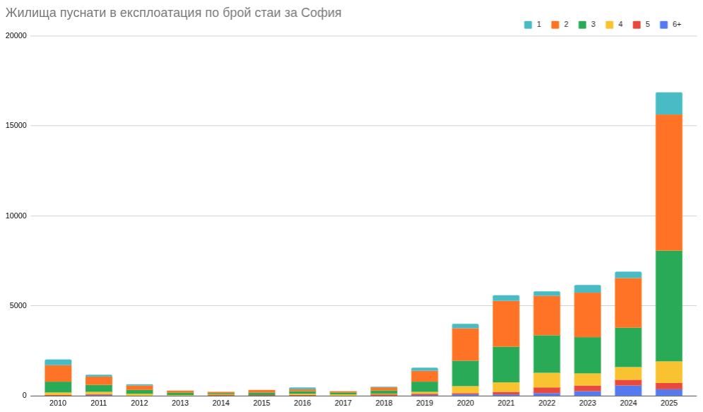
Гледайки разпределението по стаи, виждаме с учудване колко малко са жилищата над 4 стаи в сравнение със средното за страната. Това е индикация за повече апартаменти в София, малко от които са многостайни. Залага се много повече на двустайните.
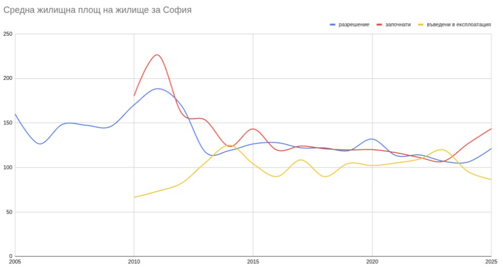
Гледайки по квадратура виждаме доближаване в последните години на това, което е разрешено и се строи и какво се декларира като площ на готовите жилища. В София се движат около 100 кв.м., но се вижда отчетливо намаление в последната година, вероятно заради строежа на повече двустайни апартаменти.
Ако искате да видите как ще изглеждат не само разрешените за строеж сгради, но и тези, които са в процес на одобрение или са планирани в бъдеще на база ОУП и стари ПУП-ове, погледнете 3D картата на потенциалното застрояване на София. Доколкото тук говорим за нови жилища, опитах се да направя анализ колко стари са се продали миналата година фокусирайки се най-вече върху панелките.
Пловдив
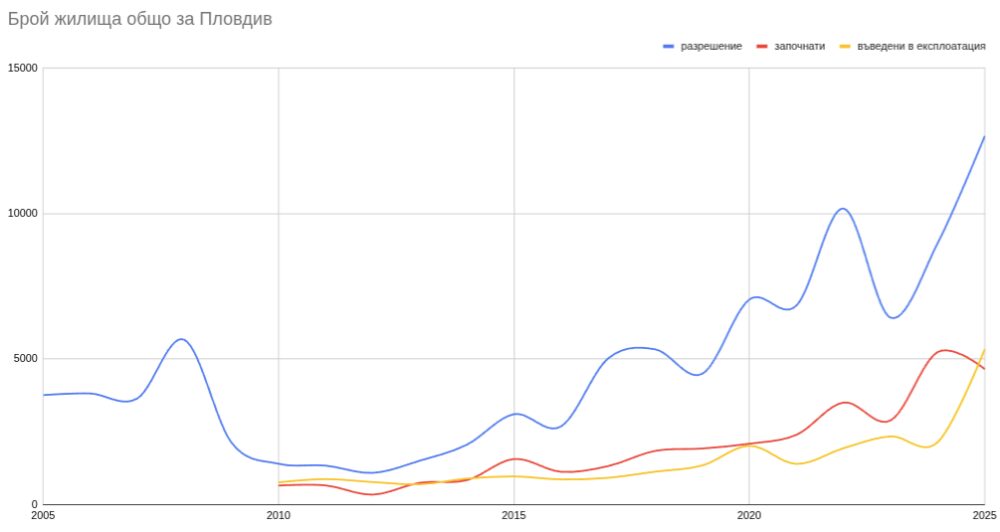
Картинката в Пловдив е доста различна. Отново виждаме скок в последната година и леко намаление в новите строежи. Виждаме обаче стремглав ръст в разрешенията за строеж, особено в мандата на сегашния кмет. Всъщност, миналата година при три пъти по-малко население в Пловдив е имало повече разрешени за строеж жилища от София – 12666 спрямо 12484. Това значи, че при липса на срив в имотния пазар в следващите 4-5 години в Пловдив в гарантирано строителство в пъти повече, отколкото виждаме в момента.
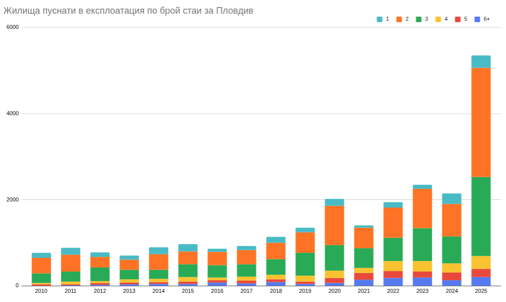
Като брой стаи не виждаме особено по-различна картинка от София. Забелязват се значително повече жилища с 6 и повече стаи. Големият брой двустайни жилища обаче следва същата логика на инвеститорите, а не купувачите.
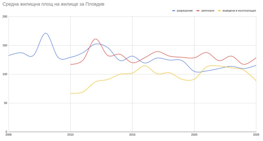
Като квадратура се вижда аналогична крива на София, но през последните години – дори по-големи жилища. Готовите жилища между 2021 и 2024-та са били средно около 111 кв., макар само 86 от тях да са били реално жилищна площ.
Благоевград
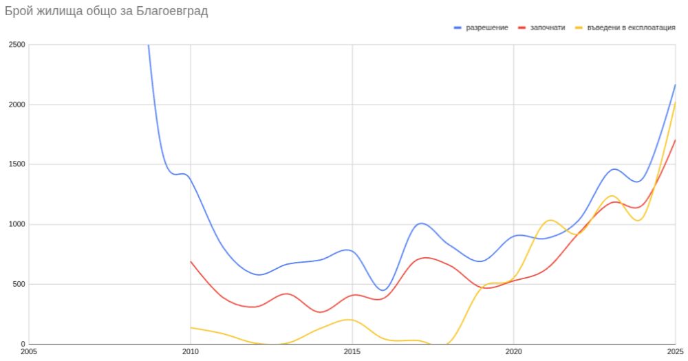
В разрешенията за строеж на Благоевград и още няколко области има аномалия, за която ще стане дума след малко. Вижда се обаче, че разрешенията за строеж, започнатите сгради и готовите жилища вървят в синхрон и със стабилен строеж в последните години. Учуди ме колко много жилища са били пуснати в експлоатация миналата година на фона на малкото население на областта.
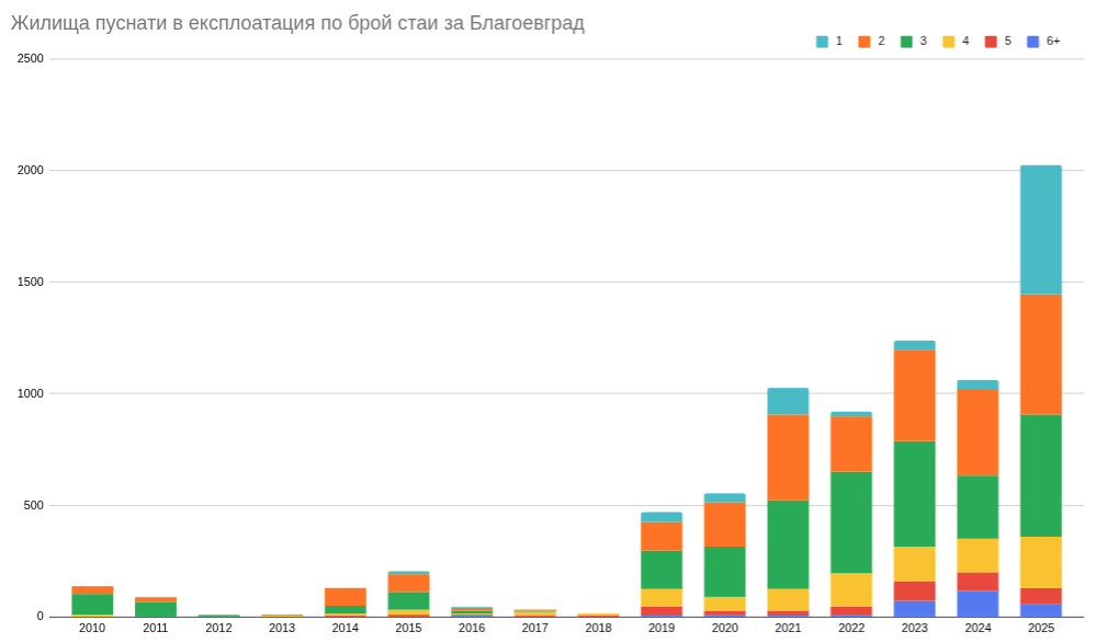
Като брой стаи виждаме изключително много едностайни. Вероятно това се дължи на самият град Благоевград, както и курортните селища, където има много жилища с цел отдаване под наем. Учудващо малко са жилищата с 4 и повече стаи, които ми говори, че се строят малко нови къщи.
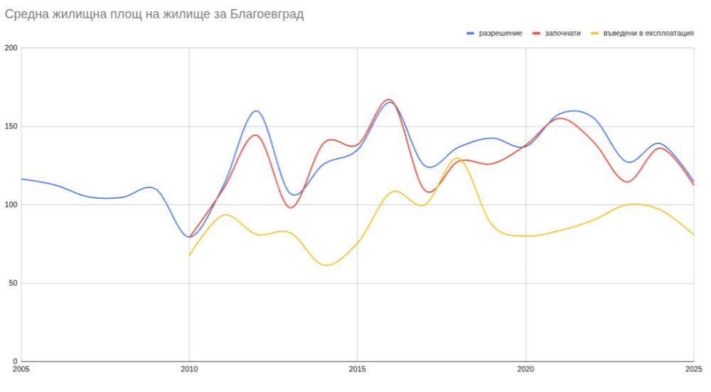
За разлика от Пловдив и София тук площта на готовите жилища е доста под 100 кв. м. и под полученото разрешение. Виждаме също спад през последната година, но като цяло виждаме, че в последните 20 се строят по-малки жилища. Това е странно предвид, че земята далеч не е толкова скъпа, колкото в други градове.
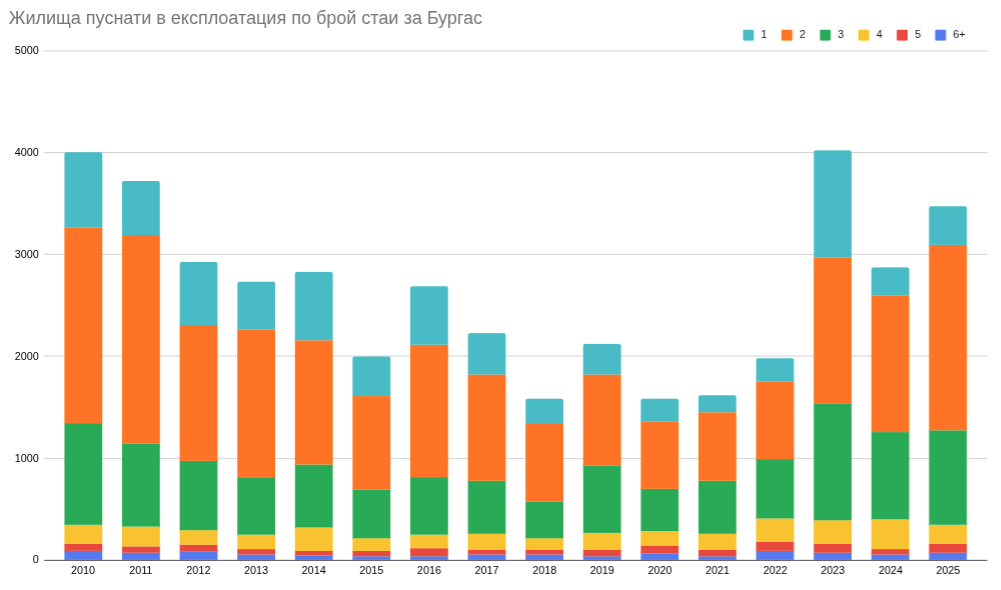
Бургас
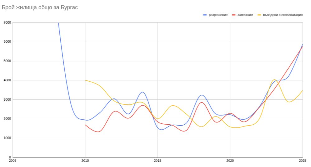
Виждаме аналогичен на Благоевград ръст на разрешенията и започнатите строежи, но спад в пуснатите в експлоатация жилища. Тук интересното е, че има много ниско ниво на строителство между 2010-та и 2022-ра спрямо населението. Също аналогично има аномалия в разрешенията за строеж преди 2008-ма.
От гледна точка на броят стаи, виждаме доста едностайни жилища през годините с пик през 2023-та. В последните две дори са по-малко спрямо предишни години. Доста малко многостайни апартаменти като дял от всички в сравнение с други области.
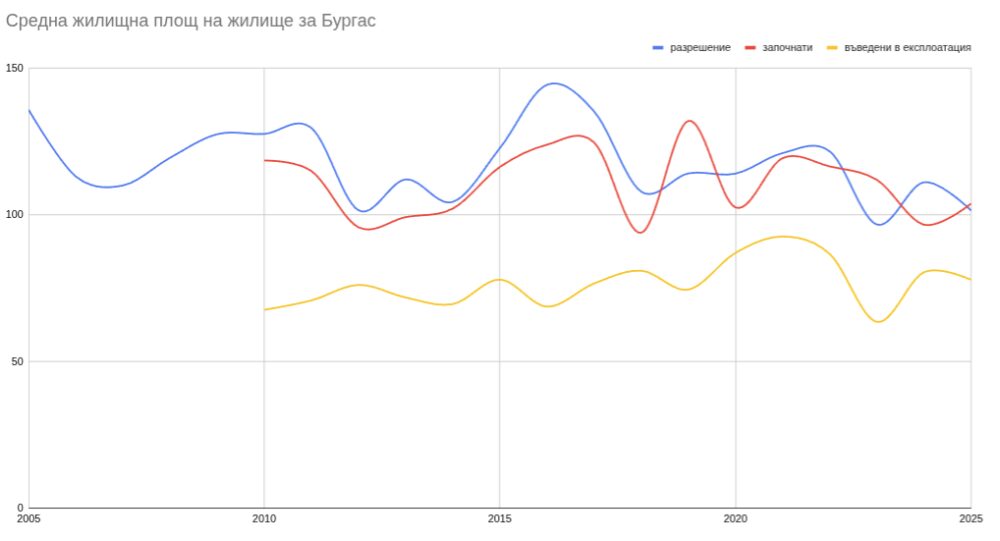
От гледна точка на жилищната площ виждаме относително постоянство в Бургас. Доста по-ниско е от Пловдив и дори Благоевград и след кратък скок на готовите жилища през 2021-ва се вижда отново спад. Предвид колко малко жилища са били пуснати на пазара тогава, възможно е да е имало един или няколко по-големи комплекса с големи жилища, които еднократно да са отместили статистиката. Съдейки по разрешенията и започнатото строителство, изглежда същите са били строени поне 4 години.
Варна
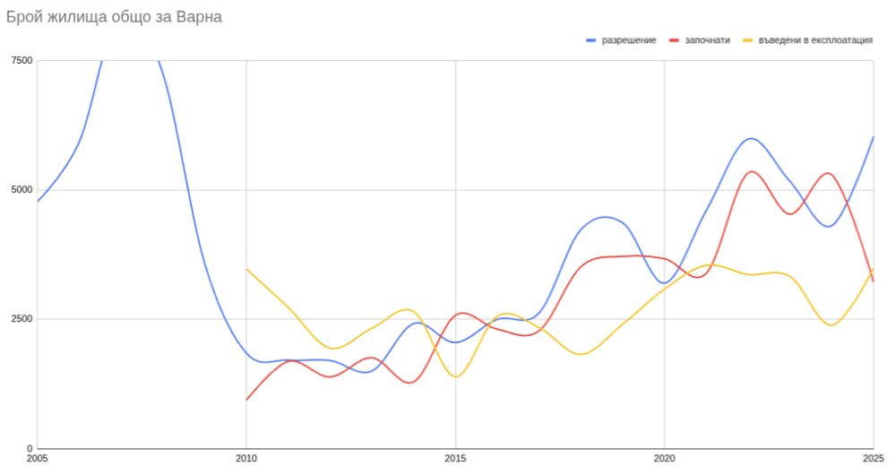
За разлика от Бургас, във Варна има значително по-голямо строителство и то постепенно расте в последните години. Разрешенията за строеж и започнатите сгради са се удвоили за последните 10 години. За разлика от други градове пуснатите в експлоатация жилища ги следват доста точно, което може да значи, че по-малко биват изоставяни или без акт 16.
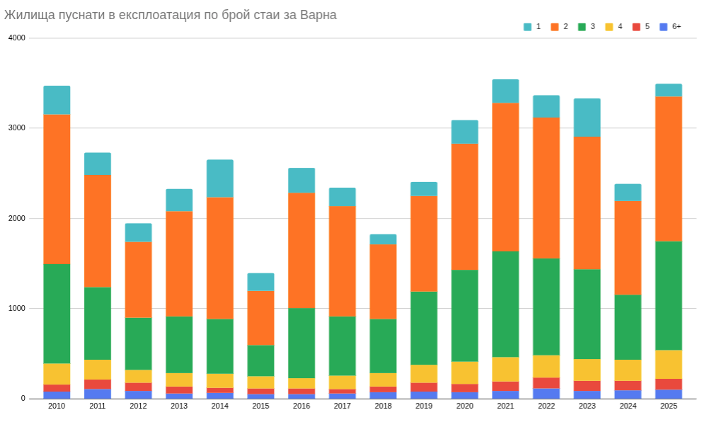
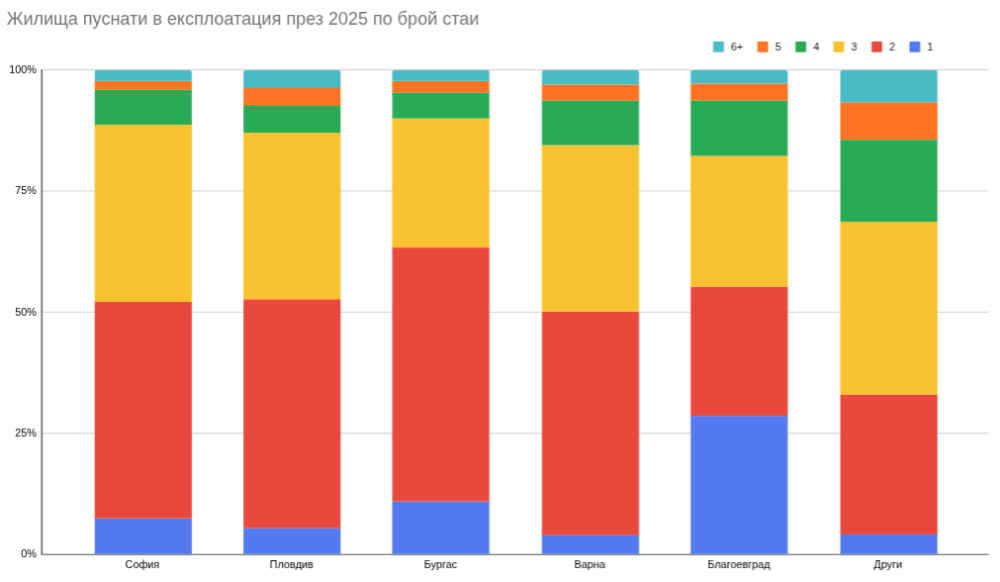
За разлика от Бургас има доста по-малко едностайни апартаменти и повече многостайни с 4 и повече стаи. Това е странно предвид, че и двата града са курортни и би било логично да се търсят повече апартаменти за отдаване под наем.
Като квадратура отново средното ниво е стабилно и доста под това в други области аналогично на Бургас. Разликата е, че всъщност разрешенията и започнатото строителство е с тенденция надолу, което значи, че в блузките години ще виждаме все повече жилища с реална площ от по 60 кв. м. във Варна описвани в рекламите като 100 кв.
Сравнение
Ако сравним разпределението по стаи на жилищата довършени през 2025-а г. виждаме големи разлики. Взимам отново 5-те града с най-много жилища пуснати в експлоатация. Пловдив, Варна и София са доста близки, макар да се виждат повече многостайни в Пловдив и Варна – вероятно къщи. Благоевград има много едностайни, което говори за апартаменти под наем. Виждат се и доста повече многостайни като дял от други области, което вероятно пак са къщи по подобие на дялът в „други“. Бургас е някъде по средата между Варна и Благоевград.
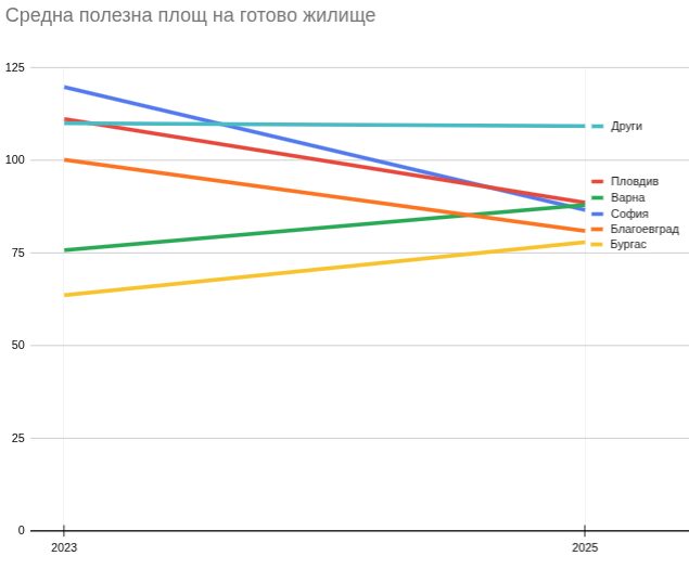
От гледна точка на площта, виждаме намаление при Пловдив, Благоевград и София между 2023 и 2025-та и увеличение при Варна и Бургас. Това може да зависи от вида жилища и големи проекти за комплекси, които са били довършени в дадените години. Може и да показва тенденция в местните пазари.
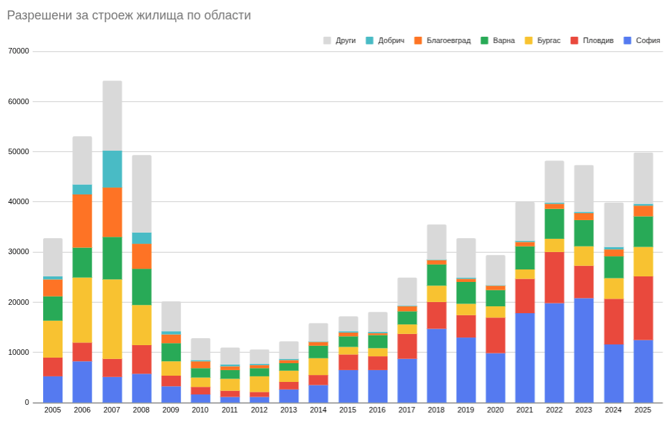
Споменах аномалии в статистиката за някои области що се отнася до разрешителните за строеж. Тук виждаме разбивката по брой жилища и избрани области. Виждаме колко много има в Бургас през 2006 до 2008-ма също както във Варна и Благоевград. Аналогичен сигнал виждаме в останалата част от страната, макар и не толкова драматично. Интересно е, че специално 2007-ма в Добрич е имало повече разрешения за строеж като брой жилища, отколкото следващите 18 години. Единствено Пловдив изглежда като изключение от областите по този показател.
Пазар за жилища или криптобетон
Споделял съм доста мнението си, че голяма част от строителството е това, което аз наричам „криптобетон“, т.е. спекулативен инструмент, а не материална собственост, която се използва по предназначение. Доколкото дигиталните инструменти като криптовалута и NFT-та нямат материално изражение, а апартаменти, офиси и прочие имоти могат да бъдат използвани теоретично в някакъв момент, важно е да разберем какво точно се крие в тази дума „теоретично“.
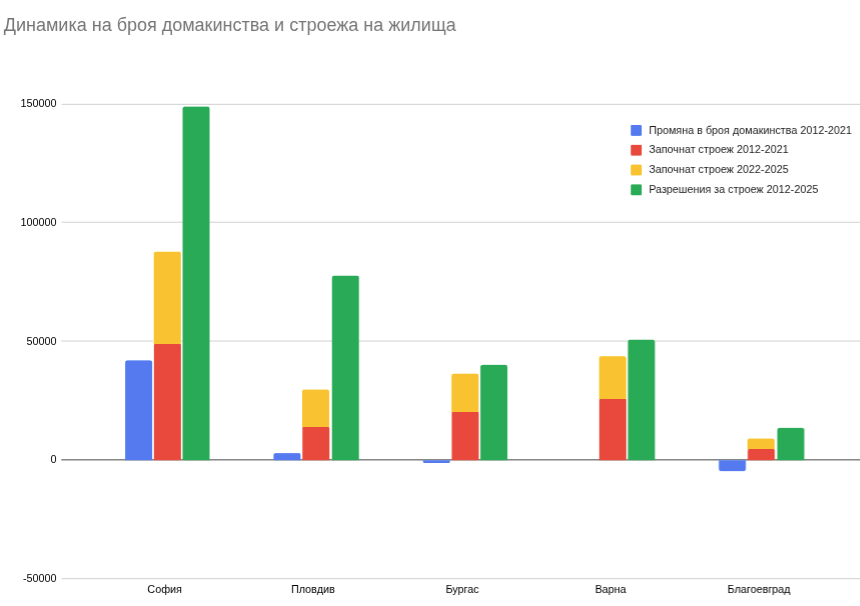
Отново данните на НСИ показват, че броят на домакинствата е намалял с 139 хиляди между двете преброявания през 2011 и 2021 г. Това е около 4.6% по-малко. Тук е важно да се разбере, че намалението на населението не се отразява пряко на броя домакинства. Възможно е при намаляващо население да има повече домакинства, какъвто е случая между преброяванията през 2001-ва и 2011-та, когато са отбелязани 83700 повече домакинства, но при 552 хиляди по-малко население. Причината за това е, че домакинствата стават по-малки – повече хора живеят отделно от родителите си, имат по-малко деца или живеят сами.
При 139 хиляди по-малко домакинства виждаме 208 хиляди жилища получили разрешение за строеж в периода между двете преброявания – 2012 и 2021 г. Също така за този период е започнал строежа на 135 хиляди жилища. 104 хиляди са били пуснати в експлоатация. Тези числа не бива да се събират, защото доста сгради са получили разрешение за строеж и са били довършени в рамките на тези 10 години.
По-интересно е обаче да се види разбивка по райони, защото демографската картина е различна. София е станала емблематична с масовото си застрояване. Данните от преброяванията дават аргумент защо пазарът би търсил повече жилища – домакинствата са се увеличили с почти 42 хиляди за 10 години. Това би означавало значително търсене на имоти. За същия период обаче 49 хиляди жилища са започнали строеж. В последните 4 години след преброяването още 39 хиляди жилища са също в строеж. Общо от 2012-та насам близо 149 хиляди жилища са получили разрешение за строеж, което е над два пъти и половина повече от най-оптимистичните прогнози за увеличението на домакинствата.
В Пловдив също има увеличение с 2841 домакинства между преброяванията, но за същия период са били започнати над 14 хиляди жилища. В последните 4 години – още 16 хиляди. Разрешенията за строеж от 2012-та насам са за 77 хиляди жилища. Това значи почти 20 пъти най-оптимистичните прогнози за увеличение на домакинствата.
В Бургас и Варна имаме леко намаление – съответно с 1230 и 221 домакинства. Въпреки това за тези 10 години е започнат строеж съответно на нови 21 и 26 хиляди жилища и още 16 и 18 хиляди отгоре в следващите 4. Разрешенията за строеж в последните 14 г. са за 40 хиляди жилища в Бургас и 51 хиляди във Варна при намаляващ брой домакинства. Предвид, че говорим за областите като цяло, там може да се спори, че става дума за ваканционни къщи и апартаменти. Предвид броя им и динамиката на населението обаче, неизменно повечето ще са с инвестиционна цел.
В Благоевград има намаление от близо 5000 домакинства, което е свиване с 4%. Въпреки това е започнал строеж на 4800 жилища между 2012 и 2021-ва и още 5000 след това. Общо 88 хиляди жилища са били разрешени за строеж в последните 14 г. Доколкото тук може отново да говорим за търсене на ваканционна къща и апартамент, особено около района на Банко и Гоце Делчев, все пак говорим за разлика от над 16 хиляди жилища между започнатите такива и очакваното намаление на домакинствата за този период.
Останалите области в България не ги виждате на графиката, тъй като там намалението е най-драматично. Виждаме 177 хиляди домакинства по-малко извън изброените горе между преброяванията. В същото време има 38 хиляди повече построени жилища за същия период и още 28 хиляди – след това. Разрешенията за строеж след 2011-та са 88 хиляди въпреки рязко намаляващия брой домакинства.
Running a large-scale ad-serving infrastructure presents unique challenges when balancing tenant isolation with operational efficiency. Our infrastructure handles millions of requests per second and generates billions of dollars in annual advertising revenue, serving ads across multiple properties and systems.
The cellular architecture problem
Earlier, we had a cellular architecture where we allocated each AWS account with Application Load Balancer (ALB) and Amazon Elastic Container Service (Amazon ECS) to a given tenant. This approach provided accurate isolation but created the following significant operational challenges.
The scale problem: Supporting only 18 clients across four AWS Regions requires 181 separate targets. Our team configured dedicated AWS accounts, VPCs, load balancers, AWS Identity and Access Management (IAM) roles, and downstream service connections for each client.
The efficiency problem: Our servers spent more than 98 percent of their time waiting and less than 1 percent executing code. Average CPU utilization sat at 3 percent, and memory at 19 percent. We were paying for massive infrastructure that remained idle most of the time.
The onboarding problem: Bringing a new client online took approximately 52 days—roughly two weeks for AWS account provisioning, three weeks for VPC and networking setup, one week for IAM role configuration, and two weeks for downstream service integration and testing.
The scalability problem: When traffic grows or a new client joined, our only option is to spin up an entirely new cell and migrate to the client. We couldn’t support concurrent tier-1 live events—multiple high-value games couldn’t run simultaneously, forcing us to divert traffic to alternative systems.
The noisy neighbor problem: Despite our isolation efforts, we still experienced performance degradation when tenants shared infrastructure, affecting service quality and reliability.
Why we needed dedicated compute
Our ad-serving platform is a stateful service that loads and maintains data in memory for each tenant rather than fetching it from a database on every request. This in-memory state improves performance but creates the noisy neighbor problem when tenants share infrastructure.When two tenants share a cluster, their in-memory data competes for the same heap. A tenant with a large dataset can trigger out-of-memory conditions that affect its neighbors. This made shared-task and shared-cluster approaches challenging our stateful workloads.We needed a solution that maintained cluster-level isolation while dramatically improving operational efficiency.
Solution overview
We designed a hybrid multi-tenant architecture that provides cluster-level isolation within shared accounts. Here’s what we implemented:
Pre-integration model: Instead of provisioning VPCs, IAM roles, and downstream service connections for each new tenant, we created a configuration-driven infrastructure where these integrations are established once and reused across tenants.
Amazon Route 53 weighted routing: We implemented Route 53 weighted routing to enable gradual traffic migration between clusters without client-side changes. This allowed us to shift tenants between tiers as their traffic patterns evolved.
AWS PrivateLink connectivity: We established AWS PrivateLink endpoints that all tenants share, removing the need for us to set up new VPC peering or Transit Gateway connections for each tenant and reducing network configuration overhead by 80 percent.
Tier-based architecture: We organized our infrastructure into tiers (High TPS, Standard TPS, Low TPS) with multiple cells per tier, enabling horizontal scaling without the operational burden of per-tenant AWS accounts.
Configuration-driven onboarding: New tenant onboarding became a configuration change rather than an infrastructure provisioning exercise, dramatically reducing time and manual effort.
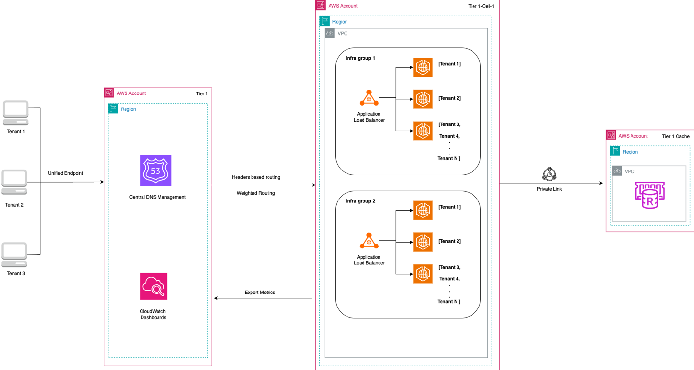
The architecture is organized around three nested levels of hierarchy. A tier is the top-level grouping—a logical classification of tenants that share a common infrastructure footprint. A tier spans one or more cells, where each cell is an AWS account boundary that represents the unit of horizontal scale-out at the account level. Within each cell, one or more infra groups serve as the self-contained infrastructure unit: a VPC, an Application Load Balancer, a set of ECS clusters (one per tenant), IAM roles, and a monitoring stack.
Why three levels? As you scale from 10 to 100 to 1,000 tenants, you will reach different AWS limits at different scales. Application Load Balancer target group limits constrain how many tenants fit in a single load balancer. AWS account limits on Elastic Network Interfaces (ENIs) and VPC endpoints constrain how many load balancers fit in a single account. This three-level hierarchy gives you two independent scaling levers to address each constraint—add infra groups to scale within an account and add cells to scale across accounts. The key design principle is that we pre-wire downstream service dependencies at tier creation, not at tenant onboarding. AWS PrivateLink connections from the tier VPC to each downstream service VPC are established after the tier is provisioned. After onboarding tenants to that tier, they automatically inherit full downstream connectivity. This single architectural decision is the primary reason for the 80 percent reduction in infrastructure setup steps. Route 53 performs weighted DNS routing across Application Load Balancers in multiple infra groups and cell accounts, enabling horizontal scale-out without client-side changes.
The following diagram illustrates the full architecture: Route 53 distributes traffic across ALBs in multiple infra groups within a single cell account, each ALB routes to tenant-specific ECS clusters using listener rules and target groups, and the clusters share tier-level PrivateLink connections to downstream services.
Figure 1: Hybrid multi-tenant architecture showing Route 53 weighted routing, Application Load Balancer listener rules, dedicated ECS clusters per tenant, and shared AWS PrivateLink connections to downstream services.
Prerequisites
Before you build this architecture, make sure that you have the following:An AWS account configured with least privileged permissions to create VPCs, Application Load Balancers, ECS clusters, Route 53 hosted zones, and VPC endpoints. You also need the AWS Command Line Interface (AWS CLI) version 2.x or later installed and configured with appropriate credentials. This walkthrough assumes intermediate familiarity with Amazon ECS, Application Load Balancer, and Amazon Route 53—specifically ECS task definitions, Application Load Balancer listener rules, and Route 53 routing policies. You also need at least one downstream service exposing a VPC endpoint service for AWS PrivateLink connectivity.
Estimated time to complete: 2–3 hours.
Walkthrough
This walkthrough shows you how to build the previously described hybrid multi-tenant architecture. You will configure Route 53 weighted routing, deploy an ALB with tenant-specific listener rules, create dedicated ECS clusters per tenant, and establish AWS PrivateLink connectivity to shared downstream services. These will be done in a way that makes future tenant onboarding a configuration-only operation.
Step 1: Configure Route 53 Regional endpoints with weighted routing
Each tier exposes a single Regional DNS endpoint (for example, tier-1.us-east-1.example.com) backed by Route 53 weighted routing records. You can configure Route 53 to use weighted routing to help distribute traffic across ALBs in multiple AWS accounts. When you add a new account to the tier for horizontal scale-out, add a new weighted record. You don’t need to change existing tenant DNS entries.
To configure Route 53 weighted routing for a tier:
Open the Amazon Route 53 console and choose Hosted zones.
Select or create the hosted zone for your tier.
Choose Create record and select Weighted as the routing policy.
Set the record name to your tier endpoint (for example, tier-1.us-east-1.example.com), record type to A, and configure an alias pointing to the ALB in your first AWS account.
Set the Weight to 50 and provide a unique Set ID (for example, account-1).
Enable Evaluate target health so Route 53 helps make sure that it directs traffic to healthy ALBs when you configure health evaluation.
Repeat for each additional AWS account in the tier, using matching weights.
Alternatively, run the following AWS CLI command to create the first weighted record:
Route 53 supports up to 10,000 weighted records per hosted zone, so this approach scales to thousands of AWS accounts without architectural changes. For more information about weighted routing, see Weighted routing in the Amazon Route 53 Developer Guide.
Step 2: Deploy an Application Load Balancer with tenant-specific listener rules
Each infra group contains one Application Load Balancer. The load balancer inspects incoming requests and forwards them to the correct tenant’s ECS service based on a tenant identifier extracted from the request path or a custom HTTP header.
Two Application Load Balancer quotas shape the capacity of each infra group: a maximum of 100 target groups per load balancer, and a maximum of 5 target groups per listener rule. With 20 listener rules each forwarding to 5 target groups, a single load balancer supports up to 50 tenants per infra group. With up to 5 ECS clusters per tenant, a single infra group can host up to 100 ECS clusters.
To create a tenant-specific listener rule:
Open the Amazon EC2 console and choose Load Balancers in the navigation pane.
Select your Application Load Balancer and choose the Listeners tab.
Choose View/edit rules for the HTTPS listener.
Choose the plus (+) icon to add a new rule.
Add a condition: Path is /tenant-a/* (or HTTP header if you use header-based routing).
Add an action: Forward to the target group for tenant-a.
Set a unique rule priority and save.
To create the target group and listener rule using the AWS CLI:
# Create a target group for the tenant
aws elbv2 create-target-group \
  --name tg-tenant-a \
  --protocol HTTP --port 8080 \
  --vpc-id YOUR_VPC_ID \
  --target-type ip
# Add a listener rule routing /tenant-a/* to the target group
aws elbv2 create-rule \
  --listener-arn YOUR_LISTENER_ARN \
  --conditions '[{"Field":"path-pattern","Values":["/tenant-a/*"]}]' \
  --actions '[{"Type":"forward","TargetGroupArn":"YOUR_TARGET_GROUP_ARN"}]' \
  --priority 10
In this step, you create a dedicated ECS cluster for each tenant within your infra group’s VPC. Use a consistent naming convention that encodes the tier, cell, infra group, and tenant identifier (for example, tier-1-cell-1-ig-1-tenant-a) to make ownership clear during operations and incident response.To create a dedicated ECS cluster for a tenant:
Open the Amazon ECS console and choose Clusters.
Choose Create cluster.
Enter a cluster name following your naming convention (for example, tier-1-cell-1-ig-1-tenant-a).
Select EC2 Linux + Networking and configure the instance type and Auto Scaling group settings appropriate for the tenant’s workload.
In the ECS task definition for this tenant, pass the tenant identifier as an environment variable. The application reads this value at startup to scope its data access — loading only that tenant’s configuration and state from the shared remote cache:
Note: Replace your-ecr-image:latest with your Amazon Elastic Container Registry (Amazon ECR) image URI.
Register the ECS service as a target in the ALB target group created in Step 2. Configure ECS service auto-scaling based on central processing unit (CPU) and memory utilization metrics, scoped to the individual service. Because each cluster is single-tenant, the ECS limit of 5,000 tasks per service applies exclusively to that tenant. One tenant’s resource consumption can’t affect another tenant’s cluster. For more information, see Creating a cluster in the Amazon ECS Developer Guide.
Step 4: Establish AWS Private Link connectivity to shared dependencies
This step happens at tier creation, not at tenant onboarding—and that distinction is the architectural heart of the design. For each downstream service your application integrates with, create a VPC interface endpoint in the infra group VPC. The ECS tasks in the tier route traffic to downstream services through these endpoints. Tenants onboarded to that tier can access downstream connectivity through the pre-configured endpoints.
Each VPC interface endpoint costs approximately $7.30/month plus data transfer charges ($0.01/GB). For a tier with 50 tenants sharing one endpoint, this cost is negligible compared to the operational savings. If your downstream services are in the same VPC, consider using VPC peering or AWS Transit Gateway as lower-cost alternatives. Use AWS PrivateLink when you need to connect to services in different AWS accounts or when you require the security and isolation benefits of private connectivity.
To create a VPC interface endpoint for a downstream service:
Open the Amazon VPC console and choose Endpoints in the navigation pane.
Choose Create endpoint.
Select Find service by name and enter the VPC endpoint service name provided by the downstream service owner.
Select the infra group VPC and the subnets used by ECS tasks.
Attach a security group that allows outbound traffic from ECS tasks to the endpoint on the required port.
Define tier-level IAM roles with the permissions needed to access downstream services and assign these roles to ECS task definitions at the tier level. New tenants can receive the tier-level permissions through the shared IAM roles without per-tenant role creation. For more information, see Access an AWS service using an interface VPC endpoint.
Step 5: Configure tenant isolation, scaling, and observability
This architecture enforces tenant isolation at three layers through customer configuration. At the routing layer, ALB listener rules route traffic exclusively to the correct tenant’s target group based on the tenant identifier. ALB listener rules help route traffic to the correct tenant’s target group based on your configuration. At the compute layer, each tenant has a dedicated ECS cluster, so resource limits apply per cluster and cluster-level isolation is designed to help minimize the impact of one tenant’s resource consumption on another tenant. At the in-memory state layer, because each ECS cluster is single-tenant, in-memory data loaded at startup belongs exclusively to that tenant with no shared heap between tenants.
Scaling strategies
When a single tenant’s traffic grows but you haven’t reached the 50-tenant limit per infra group, use vertical scaling — it’s faster (minutes vs. hours) and doesn’t require Route 53 changes. Increase ECS task CPU and memory reservations in the task definition, or switch to larger EC2 instance types in the Auto Scaling group.
When you’re approaching the 50-tenant limit or when multiple tenants need capacity simultaneously, add a new infra group within the same cell—a new VPC, ALB, and set of ECS clusters. Route 53 weighted routing distributes traffic across infra groups without client-side changes:
Use cell-level scaling only when you’re approaching account-level limits—typically after 3–4 infra groups per cell. Each AWS account has hard limits on ENIs, VPC endpoints, and other resources. When a cell approaches these limits, add a new cell by provisioning an identical tier infrastructure stack in a new AWS account and registering its ALBs in Route 53 with weighted records alongside existing cells:
The tier endpoint (tier-1.us-east-1.example.com) remains stable. Tenants don’t need to update their DNS configuration as the tier grows. The following table summarizes when to use each scaling lever:
Trigger
Action
Unit added
Application Load Balancer target group limit (~50 tenants per infra group)
Add an infra group within the same cell
Infra group (VPC + Application Load Balancer + ECS clusters)
AWS account-level limits (ENIs, VPC endpoints)
Add a new cell
Cell (new AWS account)
Observability
Observability is structured at two levels. Emit tenant-level metrics from each ECS service with the tenant identifier as an Amazon CloudWatch dimension. Key metrics to monitor:
Memory usage per ECS service is the primary signal for in-memory state growth. A sudden spike often indicates a data model change or misconfigured data pipeline. Set CloudWatch alarms at 70 percent (warning) and 85 percent (critical). When memory usage exceeds 70 percent, investigate whether the tenant’s data model has changed or if a data pipeline is misconfigured. At 85 percent, prepare to vertically scale the ECS task definition. TargetResponseTime and request count per ALB target group measure latency and throughput per tenant. Establish a baseline for each tenant during onboarding (typically 100–200 ms for stateful services), then alert when latency exceeds 2x baseline for more than 5 minutes. HTTPCode_Target_5XX_Count per target group tracks error rate per tenant.For tier-level health, monitor ALB ActiveConnectionCount and ProcessedBytes, Route 53 health check status per load balancer, and ECS cluster CPU reservation and memory reservation for capacity planning. Configure Amazon CloudWatch Logs with structured log fields including tenant_id, tier_id, and region in every log entry. Use a single log group per tier with log stream prefixes that encode the tenant identifier. The following CloudWatch Logs Insights query identifies error rates by tenant across the entire tier:
fields @timestamp, tenant_id, @message
| filter @message like /ERROR/
| stats count() as error_count by tenant_id
| sort error_count desc
Step 6: Validate the architecture
Before onboarding production tenants, validate your architecture with the following checks:
Send test requests to your tier endpoint with different tenant identifiers in the path.
Verify that Route 53 distributes traffic across Application Load Balancers: aws route53 test-dns-answer --hosted-zone-id YOUR_ID --record-name tier-1.us-east-1.example.com
Confirm the load balancer routes requests to the correct tenant’s ECS cluster by checking ALB access logs.
Test AWS PrivateLink connectivity by making requests from ECS tasks to downstream services.
Simulate a tenant memory spike by loading a large dataset and confirm that it doesn’t affect other tenants.
Verify that CloudWatch metrics are being emitted with correct tenant_id dimensions.
Results
These results come from implementing this architecture for a stateful ad-serving application. Before this architecture, onboarding a new tenant required 52 days. With this architecture, onboarding dropped to seven days—primarily testing and validation, because infrastructure is pre-provisioned.
Measured improvements:
Tenant onboarding time: from 52 days to 7 days (86 percent reduction)
Infrastructure setup steps per tenant: 80 percent fewer
Engineering effort per onboarding: 80 percent reduction
Feature release time: from 2–3 days to 1 day
Tenant capacity: up to 100 tenants per AWS account with strong cluster-level isolation
Cleaning up
To avoid incurring future charges, delete the resources in the following order:
Deregister ECS services from target groups, then delete ECS clusters (this might take 5–10 minutes).
Delete Application Load Balancer listener rules, then delete target groups associated with test tenants.
Remove Route 53 weighted routing records for test tier endpoints.
Delete VPC interface endpoints (AWS PrivateLink) created during tier setup.
Terminate EC2 instances in Auto Scaling groups, then delete the Auto Scaling groups.
(Optional) Delete the VPC if no other resources depend on it.
Note: Deleting these resources stops charges immediately. If you plan to reuse this architecture, consider stopping ECS services instead of deleting clusters.
Conclusion
In this post, I showed you how to build a hybrid multi-tenant architecture that provides strong tenant isolation without requiring per-tenant AWS accounts. You learned how to configure Route 53 weighted routing to distribute traffic across multiple accounts, deploy Application Load Balancer listener rules for tenant-specific routing, create dedicated ECS clusters per tenant, and establish AWS PrivateLink connectivity to shared dependencies. This approach reduced tenant onboarding time by 86 percent and infrastructure setup steps by 80 percent.
The most important design decision is decoupling dependency setup from tenant onboarding. Pre-wiring the PrivateLink connections, IAM roles, and remote cache endpoints at tier creation transforms onboarding from a multi-week infrastructure project into a configuration-only operation. The three-level hierarchy (tier, cell, infra group) gives you two independent scaling levers. Add infra groups when an Application Load Balancer approaches its target group limit. Add cells when an AWS account approaches its ENI or VPC endpoint limits. Route 53 weighted routing absorbs both changes transparently.
Next steps
Ready to implement this architecture? Here’s how to get started:
Assess your current tenant distribution and identify candidates for tier consolidation.
Define tier promotion criteria based on your latency and isolation requirements.
Start with a single tier and 2–3 test tenants to validate the architecture.
Gradually migrate existing tenants using a phased approach.
Monitor tenant-level metrics for 2–4 weeks before scaling to additional tiers.
After you’ve implemented this architecture, consider these additional improvements: formalized tier migration playbooks with automated tooling to make moving tenants between tiers a predictable, low-risk operation; and bin-packing analysis across tiers to identify tenants whose memory footprints allow co-location on the same EC2 instance without sharing a cluster, reducing EC2 costs while maintaining isolation properties.Have you implemented a similar multi-tenant architecture? Leave a comment or reach out to share your story.
As a general rule, when developers talk about huge pages, they are
referring to PMD-level pages that are 1MB or 2MB in size, depending on the
CPU architecture. Most CPUs can support other huge-page sizes, though. On
x86 systems, PUD-level huge pages hold 1GB of data. Providing such large
pages transparently to processes has generally not been considered as
either feasible or desirable, but Usama Arif is trying to change that
assessment. At the 2026 Linux Storage,
Filesystem, Memory Management, and BPF Summit, he led a session in the
memory-management track on how to make transparent huge pages (THPs) truly
huge.
Sabeen Malik is VP, Global Government Affairs and Public Policy at Rapid7. ⠀
Security teams need a better way to connect what they detect, what they fix, and what they can prove.
The pace of modern security operations no longer works in defenders’ favor. IBM’s Cost of a Data Breach Report 2025 found that the mean time to identify and contain a breach is now 241 days, even as AI and automation help defenders move faster. At the same time, Rapid7’s 2026 Global Threat Landscape Report shows how quickly attacker behavior is compressing the response window: exploited high and critical severity vulnerabilities more than doubled year over year, increasing 105% from 71 in 2024 to 146 in 2025, while the median time from publication to CISA KEV inclusion fell from 8.5 days to 5.0 days. This is not a future risk. It is today’s operational reality.
It also exposes a governance problem most security programs were not built to solve. Security teams are expected to demonstrate, continuously, that controls are working, that risk is being reduced, and that security investments are delivering measurable outcomes. Point-in-time audit evidence, assembled quarterly, is structurally incompatible with an environment where the threat picture changes in minutes.
The underlying issue is not a lack of effort, but a disconnect. Security data lives in one place, remediation happens in another, and evidence for auditors is assembled somewhere else. When leadership asks what changed, what was fixed, and what risk remains, teams are left stitching the story together manually producing reports that reflect where the organization was, not where it is.
Cyber GRC closes that gap by bringing governance, risk management, and compliance closer to the security data and workflows teams already rely on.
Why security operations and compliance need connected data
For years, security operations and GRC have run in parallel. One team manages threats, exposures, and remediation. Another manages policies, controls, audits, and evidence. Both aim to reduce risk, but typically without shared context or shared data.
That separation is no longer sustainable. Vulnerability exploitation rose 34% year-over-year and now accounts for 20% of all breaches, with a median of zero days between critical vulnerability publication and mass exploitation (Verizon DBIR 2025). Supply chain breaches doubled, now representing 30% of all incidents. Ransomware appeared in 44% of breaches – up 37% from the prior year.
Security leaders operating in this environment face an expectation that compliance teams were not designed to meet alone: continuous proof that controls are effective against adversaries who operate at machine speed. When AI agents can autonomously chain every phase of an attack with minimal human oversight, a quarterly audit cycle is not an assurance, but a historical record.
Why Cyber GRC matters now
Boards are no longer satisfied with compliance status reports. They want dollarized risk scenarios and evidence that remediation is actually reducing exposure — not just that it was attempted.
Two pressures are converging. First, environmental complexity: modern infrastructure spans cloud, SaaS, remote endpoints, OT systems, and third-party providers. The perimeter is everywhere, and so is the attack surface. Second, regulatory expectation: SEC, NIS2, DORA, and CMMC now require demonstrable control effectiveness, not just documented policies. Both pressures demand a model that brings security activity, compliance readiness, and accountability into the same view.
What Cyber GRC changes for security and compliance teams
Cyber GRC changes how organizations use security data. Instead of disconnected, point-in-time artifacts, it enables teams to build governance and compliance workflows directly on top of real security telemetry – so evidence reflects the current state of the environment, not a snapshot assembled weeks before an audit.
In practice, this means connecting findings, controls, remediation activity, and evidence so teams can see what issues exist, who owns the response, how remediation is progressing, and what that means for overall readiness. This also helps address the compliance-theater problem directly: many programs are designed to pass audits rather than reduce actual exposure, creating false confidence and misallocated resources. Grounding compliance evidence in live security telemetry — rather than manual documentation — means teams can tell the difference between controls that are configured and controls that are working.
How connected security data strengthens compliance
Compliance has historically been treated as a separate process that happens alongside security operations. In practice, it depends on the same data. The telemetry that surfaces a critical finding also determines whether a control is operating effectively.
When evidence is generated directly from operational systems, teams spend less time assembling reports and more time improving controls. Continuous monitoring for control drift allows organizations to move from reactive audit preparation toward a consistent assurance model. Third-party risk — now a source of 30% of all breaches — benefits particularly, since continuous TPRM monitoring surfaces supply chain exposure in real time rather than at the next assessment cycle.
How Rapid7 Cyber GRC builds on existing security workflows
This shift does not require rebuilding security programs from the ground up. With the launch of Rapid7 Cyber GRC, customers can use the security data and workflows already connected through the Command Platform to support audits, assessments, and ongoing control validation. Capabilities such as HITRUST E1 control coverage provide continuous monitoring and automated evidence collection, while features like audit-ready user access exports and unified policy data reduce manual effort across SOC 2, NIST CSF, PAI, and other common frameworks.
When NIST CSF 2.0, MITRE ATT&CK, and FAIR-based risk quantification inform the evidence model rather than just the policy library, compliance becomes a byproduct of strong security operations — not a parallel burden.
Rapid7 is launching Cyber GRC to connect security operations, risk, and compliance
Organizations do not need more disconnected processes for managing risk. They need a way to connect what they detect, what they fix, and what they can prove in a way that stands up to regulatory scrutiny, board-level oversight — and keeps pace with adversaries who operate at AI speed.
That is why Rapid7 is launching Cyber GRC: to help customers bring security operations, governance, and compliance into a single, continuous view so teams can reduce risk, improve readiness, and demonstrate progress with confidence.
For current clients, reach out to your account team to get early access to Rapid7’s Cyber GRC solution and help shape what comes next.
CUBIC, standardized in RFC 9438, is the default congestion controller in Linux, and as a result governs how most TCP and QUIC connections on the public Internet probe for available bandwidth, back off when they detect loss, and recover afterward. At Cloudflare, our open-source implementation of QUIC,quiche, uses CUBIC as its default congestion controller, meaning this code is in the critical path for a significant share of the traffic we serve.
In this post, we’ll tell the story of a bug in which CUBIC’s congestion window (cwnd) gets permanently pinned at its minimum and never recovers from a congestion collapse event.
The story starts with a Linux kernel change aimed at bringing CUBIC into line with the app-limited exclusion described in RFC 9438 §4.2-12 — a fix to a real problem in TCP that, when ported to our QUIC implementation, surfaced unexpected behaviors in quiche. It has a happy ending: an elegant (near-)one-line fix that broke the cycle.
CUBIC’s logic in a nutshell
Before we dive into the core problem, a quick refresher on CCAs may help to set the stage.
The central knob a CCA turns is the congestion window (cwnd): the sender-side cap on how many bytes can be in flight (sent but not yet acknowledged) at any moment. A larger cwnd lets the sender push more data per round trip; a smaller cwnd throttles it. Every loss-based CCA, CUBIC included, is ultimately a policy for how to grow cwnd when the network looks healthy and how to shrink it when it doesn’t.
In essence, CCAs aim to maximize data transfer by inferring the “available bandwidth” of the network; because no one wants to pay for a 1 Gbps subscription and only use a fraction of it. The family of loss-based algorithms, to which CUBIC belongs, operate on a fundamental premise: (1) if there is no packet loss, increase the sending rate (i.e. increase the bandwidth utilization); (2) if there is loss, loss-based algorithms assume that the network’s capacity has been exceeded, and the sender must back off (i.e. decrease the bandwidth utilization).
This logic is built on several assumptions that have been revisited over the years. However, we’ll save that discussion for another time.
The symptom: a test that fails 61% of the time
Our investigation started with the report of unexpected failures in our ingress proxy integration test pipeline. This erratic behavior appeared in tests where CUBIC was evaluated in a scenario of heavy loss in the early part of the connection.
Recovery after congestion collapse is an uncommon regime, but it is exactly the regime a congestion controller exists to handle. Most congestion control tests exercise the steady-state and growth phases of an algorithm; far fewer probe what happens at minimum cwnd, after the connection has been beaten down. Bugs in this corner of the state space are invisible in throughput dashboards, undetectable by static review, and only surface when you deliberately drive a CCA into it and watch whether it can climb back out — which is exactly what this test did.
The simulated test setup includes the following details:
Quiche HTTP/3 client and server running at locally (localhost)
RTT = 10ms (set up in the configuration)
A 10 MB file download over HTTP/3
Using CUBIC congestion control
With 30% random packet loss injected during the first two seconds
After two seconds, loss stops entirely
The test has a generous 10-second timeout to complete the download, which is expected to be completed in four or five seconds
The expected behavior is straightforward: CUBIC should take some hits during the loss phase, reduce its congestion window, and once loss stops, steadily ramp up and finish the download well within the timeout. Instead, we observed in multiple 100-time runs that around 60% of our tests were not able to complete the download within the generous 10-second timeout.
The anomaly: 999 state transitions with zero loss
We instrumentedquiche’s qlog output with packet loss events and built visualizations to understand what was happening inside the congestion controller:
Connection overview of a failing test. After T=2s, packet loss stops entirely — yet cwnd remains pinned at the minimum floor and the congestion state oscillates between recovery and congestion avoidance every ~14ms.
After the two-second (2000 ms) mark, packet loss stops entirely. However, the number of bytes in flight remains flat, which contradicts the core logic of the CUBIC algorithm: in the absence of loss, apply more gas to increase throttle (more bytes in our world). This raises the question: if the network is no longer dropping packets, why is the congestion window failing to grow?
When we zoom into that region, our analysis shows that CUBIC enters a rapid oscillation, shown in our plot as an extended recovery phase, between congestion avoidance state (the operational regime phase) and recovery state (the packet loss recovery state) — 999 transitions in approximately 6.7 seconds. That’s one transition every ~14ms — suspiciously close to the connection’s RTT (10ms). Throughout this entire period, cwnd is locked at the minimum floor: 2700 bytes, or two full-size packets.
Clearly something in CUBIC’s logic is misinterpreting the state of the connection. The key clue is the oscillation period: ~14ms matches the RTT. Whatever is triggering the recovery/avoidance flip is happening once per round trip, in lockstep with connection’s ACK clock; the self-clocking rhythm in which each round-trip’s ACKs from the client trigger the server’s next send. Because this is a download (server to client), the ACKs in question travel client to server, and CUBIC’s state machine runs on the server side: every time those ACKs land, bytes_in_flight drops to zero and the server sends the next two-packet burst, which is what triggers the bug.
To confirm this behavior was CUBIC-specific, we ran the same test with Reno, another member of the loss-based family but with a different growth rate. The results were conclusive: 100% pass rate, showing Reno recovered cleanly after the loss phase, and revealing that this is a CUBIC-related bug.
Reno recovers cleanly after the loss phase ends at T=2s and completes the download by ~5s
Tracing the root cause
Loss-based algorithms have two pedals, gas and brake, with a difference in how they accelerate. Well, CUBIC comes with some extra features. Here we are going to focus on bytes_in_flight == 0.
TCP CUBIC after idle (Linux, 2017)
To understand the bug, we first need to understand the optimization it came from. In 2017,an issue was found with Linux kernel’s CUBIC implementation. Thecommit message explains:
The epoch is only updated/reset initially and when experiencing losses. The delta “t” of now - epoch_start can be arbitrary large after app idle as well as the bic_target. Consequentially the slope (inverse of ca->cnt) would be really large, and eventually ca->cnt would be lower-bounded in the end to 2 to have delayed-ACK slow-start behavior.
This particularly shows up when slow_start_after_idle is disabled as a dangerous cwnd inflation (1.5 x RTT) after few seconds of idle time.
The epoch is the reference timestamp CUBIC uses to anchor its growth curve: W_cubic(delta_t) is parameterized by delta_t = now - epoch_start, and the epoch is reset whenever CUBIC restarts its growth function — most notably after a loss event reduces cwnd. Between resets, delta_t grows monotonically with wall-clock time.
When an application goes idle (stops sending) for a while and then resumes, the CUBIC growth function W_cubic(delta_t) computes delta_t as now - epoch_start, as illustrated in the figure below. Since the epoch wasn’t updated during idle, delta_t is huge, producing an enormous target window — and CUBIC would immediately try to inflate cwnd to an unreasonable value.
Jana Iyengar’s initial fix was to reset `epoch_start` when the application resumes sending. But Neal Cardwell pointed out the flaw in that approach:
…it would ask the CUBIC algorithm to recalculate the curve so that we again start growing steeply upward from where cwnd is now (as CUBIC does just after a loss). Ideally we’d want the cwnd growth curve to be the same shape, just shifted later in time by the amount of the idle period.
The elegant solution, authored by Eric Dumazet, Yuchung Cheng, and Neal Cardwell, was to shift the epoch forward by the idle duration rather than resetting it. This preserves the shape of the CUBIC growth curve — just sliding it in time so that the algorithm picks up where it left off.
The port to quiche (2020)
When CUBIC was first implemented in quiche, this idle-period adjustment was ported. However, QUIC, which runs in the user space, doesn’t have TCP’s kernel-level CA_EVENT_TX_START callback. Instead, the quiche implementation checks for the idle condition inside on_packet_sent():
// cubic.rs — on_packet_sent() (simplified)
/// Updates the state when a packet is sent.
fn on_packet_sent(&mut self, bytes_in_flight: usize, now: Instant, ...) {
    // If the sending burst is restarting (i.e., bytes_in_flight was zero before this send),
    // adjust the congestion recovery start time to account for the gap in sending.
    if bytes_in_flight == 0 {
        let delta = now - self.last_sent_time;
        self.congestion_recovery_start_time += delta;
    }
    // Record the time of this send event.
    self.last_sent_time = now;
}
Where it breaks: the QUIC difference
The fix ported to quiche included a bug in the original kernel change which was fixed by a followup change to the kernel cubic module about a week later. The commit message for the second fix explains:
tcp_cubic: do not set epoch_start in the future
Tracking idle time in bictcp_cwnd_event() is imprecise, as epoch_start
is normally set at ACK processing time, not at send time.
Doing a proper fix would need to add an additional state variable,
and does not seem worth the trouble, given CUBIC bug has been there
forever before Jana noticed it.
Let’s simply not set epoch_start in the future, otherwise bictcp_update() could overflow and CUBIC would again
grow cwnd too fast.
As mentioned in the commit message, recovery start time is set during ACK processing, and the computation of the adjustment based on sent times can push the recovery start time into the future. This explains the oscillation between recovery and congestion avoidance seen on our test. The trap only consistently triggers when every incoming ACK drives bytes_in_flight all the way to zero — which in practice means cwnd has collapsed to its minimum (two packets) and the application has data ready to send another full window the moment an ACK arrives. Outside this regime, bytes_in_flight == 0 is less likely to hold on every send, so it is less likely to trigger the bug.
Why doesn’t this also happen at connection start? The bug only triggers when the connection exits slow-start and switches over to congestion avoidance. Before exiting slow-start, congestion_recovery_start_time is not set, so the buggy branch in on_packet_sent has no recovery boundary to advance. During slow start CUBIC’s cwnd grows by the same Reno-style ack-based rule shared by all loss-based CCAs — the cubic curve and its sensitivity to congestion_recovery_start_time only enter the picture once the connection is in congestion avoidance, meaning the trap needs three things at once: a real loss event to set the recovery boundary, congestion avoidance to be running, and cwnd collapsed to the two-packet floor.
The self-perpetuating recovery trap. At minimum cwnd, every ACK cycle triggers the idle period adjustment with an inflated delta.
At a minimum cwnd (two packets), the dynamics of the connection shift into a “death spiral” where the idle period optimization becomes a self-fulfilling prophecy. This trap operates in a continuous loop:
Send and ACK packets: The sender transmits the entire two-packet window. After one RTT (~14ms), both packets are ACKed, causing bytes_in_flight to drop to zero.
False idle detection: When the next burst is sent, on_packet_sent() sees bytes_in_flight == 0 and assumes the connection was idle, but it was congestion limited.
Inflated delta: The calculation uses now – last_sent_time to determine the idle duration. When the congestion window (cwnd) is at its minimum, last_sent_time is the timestamp of the start of the previous RTT cycle. Therefore, the resulting delta is approximately 14ms (the connection’s RTT + additional rounding errors). This RTT-sized delta is incorrectly applied as the “idle” time. The actual time the connection was idle (the processing gap between the last ACK arriving and the next packet being sent) is effectively 0. By measuring the full RTT instead of the true gap, the delta is inflated significantly, aggressively shifting the recovery start time forward, possibly into the future.
Perceived recovery: Because the recovery start time is now in the future, the in_congestion_recovery() check returns true for every incoming ACK. Processing of the next ACK exits recovery and sets the recovery start to the ACK time which is larger than last_sent_time, making it likely for the congestion controller to push the recovery time into the future when doing the next send.
Stagnation: Since CUBIC skips cwnd growth for any packet perceived to be in a recovery period, the window remains pinned at two packets — ensuring the pipe drains completely on the next ACK and restarting the cycle.
And this loop repeats for thousands of cycles until the accumulation of small deviations — from scheduler jitter and ACK processing variance — lets the <= boundary in in_congestion_recovery() slip behind the next packet’s send time, breaking the cycle.
The fix: measuring idle from the right moment
Fixing the death spiral involves measuring the idle duration from when bytes_in_flight actually transitioned to zero (the last ACK processed) rather than the last packet sent.
The code change
Add last_ack_time timestamp to the CUBIC state.
Update that timestamp when ACKs arrive.
Use it for the idle delta computation:
// cubic.rs — on_packet_sent()
fn on_packet_sent(&mut self, bytes_in_flight: usize, now: Instant, ...) {
    // Check if the connection was idle before this packet was sent.
    if bytes_in_flight == 0 {
        if let Some(recovery_start_time) = r.congestion_recovery_start_time {
            // Measure idle from the most recent activity: either the
            // last ACK (approximating when bif hit 0) or the last data
            // send, whichever is later. Using last_sent_time alone
            // would inflate the delta by a full RTT when cwnd is small
            // and bif transiently hits 0 between ACK and send.
            let idle_start = cmp::max(cubic.last_ack_time, cubic.last_sent_time);

            if let Some(idle_start) = idle_start {
                if idle_start < now {
                    let delta = now - idle_start;
                    r.congestion_recovery_start_time =
                        Some(recovery_start_time + delta);
                }
            }
        }
}
With the delta now reflecting the actual gap since the last ACK, the recovery boundary stops chasing the send time:
Old code: boundary advances one RTT per cycle, always landing on or ahead of the next send.
Fix: boundary barely moves; the next send lands ahead of it and cwnd grows.
For genuinely idle connections, last_ack_time is far in the past and the same expression captures the full idle duration, the original epoch-shift behavior is preserved.
Validation
With the fix applied, the 100% pass rate of our quiche testing suite was restored.
After the fix, cwnd grows along the expected CUBIC curve and the download completes in ~4-5 seconds.
We don’t worry about the losses at the end of the connection — that’s expected because we fully utilized the router’s allocated buffer. In other words, we are fully utilizing the available bandwidth in this test case.
Takeaways
“Idle” is harder to define than it sounds. Normal pipeline delays at small windows can look like idleness to simple checks.
Minimum-cwnd dynamics are a unique corner case. The bug was invisible at high speeds and only triggered after severe loss.
The fix was surprisingly small compared to the complexity of the behavior. After weeks of instrumenting qlogs and analyzing visualizations to find the root cause, the solution required changing just three lines of code. As we noted during the investigation: the effort to find the bug was massive, but the fix itself was basically one line of logic.
The fix described in this post has been contributed to cloudflare/quiche, Cloudflare’s open-source implementation of QUIC and HTTP/3. Our CCA efforts go beyond loss-based algorithms: we also use quiche’s modular congestion control design to experiment with and tune our model-based BBRv3 implementation, now enabled for a growing percentage of our QUIC deployments. Stay tuned for further updates on QUIC congestion control implementation and performance.
If you’re interested in congestion control, transport protocols, or contributing to open-source networking code, check out the quiche repository. We’re always looking for talented engineers who love digging into problems like these, please explore ouropen positions.
Sabeen Malik is VP, Global Government Affairs and Public Policy at Rapid7. ⠀
Security teams need a better way to connect what they detect, what they fix, and what they can prove.
The pace of modern security operations no longer works in defenders’ favor. IBM’s Cost of a Data Breach Report 2025 found that the mean time to identify and contain a breach is now 241 days, even as AI and automation help defenders move faster. At the same time, Rapid7’s 2026 Global Threat Landscape Report shows how quickly attacker behavior is compressing the response window: exploited high and critical severity vulnerabilities more than doubled year over year, increasing 105% from 71 in 2024 to 146 in 2025, while the median time from publication to CISA KEV inclusion fell from 8.5 days to 5.0 days. This is not a future risk. It is today’s operational reality.
It also exposes a governance problem most security programs were not built to solve. Security teams are expected to demonstrate, continuously, that controls are working, that risk is being reduced, and that security investments are delivering measurable outcomes. Point-in-time audit evidence, assembled quarterly, is structurally incompatible with an environment where the threat picture changes in minutes.
The underlying issue is not a lack of effort, but a disconnect. Security data lives in one place, remediation happens in another, and evidence for auditors is assembled somewhere else. When leadership asks what changed, what was fixed, and what risk remains, teams are left stitching the story together manually producing reports that reflect where the organization was, not where it is.
Cyber GRC closes that gap by bringing governance, risk management, and compliance closer to the security data and workflows teams already rely on.
Why security operations and compliance need connected data
For years, security operations and GRC have run in parallel. One team manages threats, exposures, and remediation. Another manages policies, controls, audits, and evidence. Both aim to reduce risk, but typically without shared context or shared data.
That separation is no longer sustainable. Vulnerability exploitation rose 34% year-over-year and now accounts for 20% of all breaches, with a median of zero days between critical vulnerability publication and mass exploitation (Verizon DBIR 2025). Supply chain breaches doubled, now representing 30% of all incidents. Ransomware appeared in 44% of breaches – up 37% from the prior year.
Security leaders operating in this environment face an expectation that compliance teams were not designed to meet alone: continuous proof that controls are effective against adversaries who operate at machine speed. When AI agents can autonomously chain every phase of an attack with minimal human oversight, a quarterly audit cycle is not an assurance, but a historical record.
Why Cyber GRC matters now
Boards are no longer satisfied with compliance status reports. They want dollarized risk scenarios and evidence that remediation is actually reducing exposure — not just that it was attempted.
Two pressures are converging. First, environmental complexity: modern infrastructure spans cloud, SaaS, remote endpoints, OT systems, and third-party providers. The perimeter is everywhere, and so is the attack surface. Second, regulatory expectation: SEC, NIS2, DORA, and CMMC now require demonstrable control effectiveness, not just documented policies. Both pressures demand a model that brings security activity, compliance readiness, and accountability into the same view.
What Cyber GRC changes for security and compliance teams
Cyber GRC changes how organizations use security data. Instead of disconnected, point-in-time artifacts, it enables teams to build governance and compliance workflows directly on top of real security telemetry – so evidence reflects the current state of the environment, not a snapshot assembled weeks before an audit.
In practice, this means connecting findings, controls, remediation activity, and evidence so teams can see what issues exist, who owns the response, how remediation is progressing, and what that means for overall readiness. This also helps address the compliance-theater problem directly: many programs are designed to pass audits rather than reduce actual exposure, creating false confidence and misallocated resources. Grounding compliance evidence in live security telemetry — rather than manual documentation — means teams can tell the difference between controls that are configured and controls that are working.
How connected security data strengthens compliance
Compliance has historically been treated as a separate process that happens alongside security operations. In practice, it depends on the same data. The telemetry that surfaces a critical finding also determines whether a control is operating effectively.
When evidence is generated directly from operational systems, teams spend less time assembling reports and more time improving controls. Continuous monitoring for control drift allows organizations to move from reactive audit preparation toward a consistent assurance model. Third-party risk — now a source of 30% of all breaches — benefits particularly, since continuous TPRM monitoring surfaces supply chain exposure in real time rather than at the next assessment cycle.
How Rapid7 Cyber GRC builds on existing security workflows
This shift does not require rebuilding security programs from the ground up. With the launch of Rapid7 Cyber GRC, customers can use the security data and workflows already connected through the Command Platform to support audits, assessments, and ongoing control validation. Capabilities such as HITRUST E1 control coverage provide continuous monitoring and automated evidence collection, while features like audit-ready user access exports and unified policy data reduce manual effort across SOC 2, NIST CSF, PAI, and other common frameworks.
When NIST CSF 2.0, MITRE ATT&CK, and FAIR-based risk quantification inform the evidence model rather than just the policy library, compliance becomes a byproduct of strong security operations — not a parallel burden.
Rapid7 is launching Cyber GRC to connect security operations, risk, and compliance
Organizations do not need more disconnected processes for managing risk. They need a way to connect what they detect, what they fix, and what they can prove in a way that stands up to regulatory scrutiny, board-level oversight — and keeps pace with adversaries who operate at AI speed.
That is why Rapid7 is launching Cyber GRC: to help customers bring security operations, governance, and compliance into a single, continuous view so teams can reduce risk, improve readiness, and demonstrate progress with confidence.
For current clients, reach out to your account team to get early access to Rapid7’s Cyber GRC solution and help shape what comes next.
Юлия Федорчук е обичана и награждавана полска авторка на стихосбирки, сборници с разкази и романи. Работата ѝ като преподавателка във Варшавския университет е свързана с критика на антропоцентричната представа за устройството на света. В научната си дейност изследва постхуманистичните и екофеминистки перспективи, подчертаващи взаимната зависимост на всички живи същества на планетата. А и крехкостта на екосистемите.
Федорчук е сред ключовите фигури в Полша, които въвеждат и популяризират понятието „екопоетика“. Но също така тя разглежда литературата като пространство, което може да възстанови връзката между човека и планетарната среда.
Последният ѝ роман „Домът на Орион“ е красив, копнежен и болезнен текст за изгубеността на съвременния човек. Прикрито мрачен, романът на Юлия Федорчук засяга теми като миграцията, отчуждението, загубата на етични ориентири, белязали последните няколко поколения. Всяка част на света е достъпна в Google Maps, звездите над нас са далечни, но свързани от хилядолетия в митологичните наративи за герои, а ние ставаме все по-самотни. Вече не сме предани нито на отколешните идеи на хуманизма, нито на любовта. Остават ни единствено кратките, единични, но спасителни актове на взаимопомощ и на човешка топлота.
В съвременната наука се говори за Overview effect при астронавтите – когато видят Земята от Космоса, това ги променя завинаги. Погледнати оттам, ние сме едно цяло – без държавни граници и разделения, върху една крехка планета в необятната Вселена. Често ефектът води и до дълбоко емоционално свързване с екологичните каузи. Как според Вас изглежда настоящето, видяно толкова отвисоко?
Не съм виждала нашата планета от такава перспектива, така че не мога да кажа! Но разбира се, вярвам, че способността ни да се свържем със Земята като с живо същество може да ни помогне да осмислим екологичната реалност – както интелектуално, така и емоционално.
А екологичната реалност е, че животоподдържащите системи на планетата са застрашени от изчерпване. Всички ние участваме в модела на тези практики на съвременния капитализъм – на извличане и изчерпване на ресурсите. Невъзможно е да излезеш напълно от тях, дори да си астронавт, но не всички носят еднаква отговорност за разрушаването на екосистемите. Хората, които плащат най-високата цена за климатичните промени и другите форми на екологична разруха, често не са тези, които значително са допринесли за щетите. А климатичните промени вече са основна причина за миграции…
Във Вашите книги се занимавате с преходното, тленното, с онова, което подлежи на разпад, но и с жилавостта на живота. Ще успеем ли да съчетаем виртуалните реалности, които обитаваме днес, с естествените природни цикли?
Не съм сигурна дали наистина „обитаваме“ виртуални реалности. Компютърният капитализъм, или „надзорният капитализъм“ (според известния термин на Шошана Зубоф1) не е толкова място, което обитаваме, колкото процес, в който ние самите се превръщаме в ресурс. Днес обект на извличане (като въглищата в добрите стари времена на индустриалната революция) е човешкото внимание. Но телата ни не са се променили. Еволюцията не напредва толкова бързо. Ние все още сме бозайници. Трябва да дишаме, имаме нужда от вода и храна, нуждаем се от сън, трябва да се грижим за душата си дори когато вниманието ни е увредено от пристрастяващите технологии.
Какво намирате за лечебно? За Ваше убежище?
Това е чудесен, но и коварен въпрос. От една страна, не вярвам, че можеш да избягаш извън света и неговите проблеми. Героинята от „Домът на Орион“ Елиза научава този факт, когато се опитва да повтори пасторалния жест на бягството „в дивото“. Това, което среща там, са всички фундаментални планетарни проблеми: климатични промени, миграции (които включват удивителна човешка издръжливост, но и трагедия, и политически сложности), среща също собствената си изтощена душа. Вярвам, че единственото място за покой е в окото на урагана, така да се каже.
От друга страна, не искам да омаловажавам идеята за почивка, защото смятам, че изтощението вече е надиндивидуален, политически проблем. Понякога ходя в гората, в Беловежката пуща, и се опитвам да живея бавно в някои моменти от деня, често сутрин, преди всички да се събудят. Обичам дългите разходки, медитацията и дълбинното четене.
„Понякога оказват помощ хора, които дори не знаят, че биха имали силата да помагат“, пишете в книгата „Домът на Орион“. Трудните времена ще ни припомнят ли идеята за солидарност?
Моля да ми простите, че ще дам малко на контра, но не мисля, че имаме нужда от понятия. Когато солидарността е понятие, когато помощта е идея, проект, който имаме, тя бързо ще се изчерпи. Това, което става в кризисни ситуации, е, че хората понякога са способни на неочаквана доброта – и да, тогава има солидарност. Мисля, че Наоми Клайн писа за това в контекста на урагана „Катрина“ (който удари Ню Орлиънс през 2005 г.). Видяхме го и в Полша в началото на пълномащабното руско нахлуване в Украйна.
Ако свържем няколко звезди на картата в произволни нови фигури, ще създадем наше тайно съзвездие. Това може ли да се приеме като метафора на метода Ви на писане?
Прекрасна метафора на това, което се опитвам да правя в писането си (или поне за един аспект от него) – така че благодаря.
Помните ли детето, което бяхте? Задавало ли си е то част от въпросите, които сега Ви вълнуват?
Детето, което бях, или по-скоро детето, което помня, беше много любопитно, изпълнено с удивление, но и доста изплашено от много неща. Прекалено чувствително дете, предполагам.
Отношението ни като общество към бежанците навярно е разпнато между дехуманизирането им и желанието ни да им помогнем. Какво остава скрито зад бодливата тел на социалните предразсъдъци и страхове?
Страхувам се, че това е твърде сложен въпрос за този формат. Хората мигрират по всякакви причини: някои бягат от войни, климатични промени или крайна бедност. Други искат по-добър живот (кой би могъл да ги вини?), трети просто искат да се движат свободно, да видят как е на друго място. Осъзнавам, че границите не могат просто да бъдат отворени, не съм толкова наивна. Но ми се струва странно, всъщност дори шокиращо, че моят европейски паспорт ми позволява да отида на различни места по каквито и да било важни или тривиални причини, а друг паспорт те прави „нелегален“. И е важно да добавя, че не всички „бежанци“ получават еднакво отношение – в европейското отношение към мигрантите има много расизъм.
Вие сте университетска преподавателка. Ще имат ли упорството младите хора да се доберат до по-безопасна версия на света? И какво наследство им оставяме?
Ще кажа нещо много противоречиво: не споделям наратива, който обвинява нашето поколение за всевъзможни злини и съчувства на младите, които сега трябва да се справят с последствията. Познавам много невероятни млади хора – любознателни, ангажирани, активни, но те сякаш са малцинство. Други млади хора обаче водят изключително консуматорски начин на живот и имат наистина слабо чувство за отговорност към каквото и да било – може би защото усещат безнадеждност или защото са толкова откъснати от физическия свят.
Понякога в аудиторията, когато говоря за неща като свободата например, студентите ме гледат, като че ли съм луда, и тези моменти са наистина обезкуражаващи. Пристрастяването към неустойчивия комфорт е силно, по-силно е у младите. Това ме тревожи.
Иска ми се да узреем за идеята, че човекът е дребна частица от екосистемата на живота. Светът е красив, нали?
Ами струва ми се, че зависи от гледната точка. Можем да кажем, че светът е грозен или ужасен, и това също ще е вярно. Екологията е трудна тема. Според мен нашата свързаност с екосистемата е прекрасна, усещането за единение с нещо повече от човешките процеси на живота ни носи облекчение от ежедневните човешки борби, има нещо дълбоко духовно в това.
Но има хора, които го намират за плашещо, и аз мога да ги разбера. Независимо как се чувстваме обаче, ние зависим от Земята, от нейния климат, атмосфера, гравитация и т.н. Тази зависимост бива неглижирана (например в политиката), а аз се опитвам да действам срещу премълчаването и скриването на този факт, като поставям нашата зависимост в центъра на писането си.
1 Книгата на Шошана Зубоф The Age of Surveillance Capitalism е преведена на български: Епохата на надзорния капитализъм. София: Дилок, 2022. – Б.р.
В неделя вечер, 19 април, докато всички следяха с изненада изборните резултати и се опитваха да разберат какво се случва, аз се чудех как ще обясня на следващия ден на чуждестранните си колеги в Европейския парламент (ЕП) в Брюксел кой точно е Румен Радев и къде се позиционира „Прогресивна България“ в европейския политически пейзаж.
От името ѝ просветеният западноевропеец, който се интересува от политика, може да остане с впечатлението, че става дума за лява партия. В ЕП третата по големина група се казва „Прогресивен алианс на социалистите и демократите“ и обединява леви европейски партии, сред които и БСП. Сред мандатоносителите на „Прогресивна България“ са Политическо движение „Социалдемократи“ и Социалдемократическата партия. Тази информация не фигурира на сайта на „Прогресивна България“, но допринася за възприемането на политическия проект като ляв. В идеологическо отношение прогресивните идеи за промяна и напредък се противопоставят на консервативните идеи за запазване на статуквото, които са представлявани от традиционната десница. Какво му е прогресивното на Радев обаче?
Ако попитаме ChatGPT къде ще позиционира „Прогресивна България“
въз основа на политическата ѝ програма, публикувана на сайта на партията, приложението за изкуствен интелект я оценява като сравнително обща: „много лозунги, малко конкретика“. Платформата комбинира социалдемократическа база, силна държава и антисистемна реторика. Социалдемократическата база идва от заявките за преодоляване на бедността (стр. 5), регулирането на монополи и картели (стр. 8), намаляването на неравенството и по-справедливо разпределение на благата (стр. 13). Ако обаче погледнем данъчната политика (плосък данък – стр. 20), пробизнес ориентацията (стр. 21) и фискалната дисциплина (ограничаване на бюджетния дефицит и контрол на дълга – стр. 20), това са десни и консервативни политики.
В задачата се пита: как леви цели ще бъдат изпълнявани с десни инструменти? За намаляване на неравенствата и преодоляване на бедността в най-бедната държава от Европейския съюз от влизането ѝ в ЕС досега ще се изискват допълнителни средства. Ако няма модел на солидарност – една от основните ценности в лявата политика – и по-високо облагане на по-високите доходи, как ще бъде намалена пропастта между хората с най-ниски доходи и тези с най-високи? Може ли „Прогресивна България“ да претендира, че е лява партия, ако не залага на обществената солидарност?
Идеята за постигане на леви цели с десни политики съвсем не е нова в България. Още през 2021 г. „Продължаваме промяната“ използва този лайтмотив, като идеята е, че ако се спрат злоупотребите в държавата и с парите от данъци се финансират социални политики, това ще бъде достатъчно, за да се повиши жизненият стандарт и да се пребори бедността. В случая всъщност нито „Прогресивна България“, нито „Продължаваме промяната“ се заявяват като леви или десни партии. Вместо това застават зад прилагането на базисните принципи на правовата държава, която събира данъци и ги инвестира в политики. Запазването на данъците ще се хареса на десните избиратели, а социалните политики – на левите и така спектърът на потенциални гласоподаватели и от двете страни се увеличава.
Като за капак, за да стане объркването между ляво и дясно при „Прогресивна България“ още по-голямо,
антисистемната реторика, посочена като характерен елемент на партията на Радев от ChatGPT, е основна характеристика на крайнодесните и крайнолевите движения в Европа. Те разчитат на противопоставянето на злите елити и онеправданото мнозинство и смятат, че единственото решение е разрушаването на съществуващата система и изграждането на нов ред, в който ще цари сигурност и правда, защото доброто най-накрая ще победи. В случая с „Прогресивна България“ тази реторика е особено печеливша заради хроничните проблеми с корупцията в България и натрупаното недоволство от предишните правителства. Прилагателното „справедлив“ например е използвано 17 пъти в програмата в най-различен контекст – от здравеопазването, през законодателството, ценовия пазар и ВиК услугите, до мира с Украйна.
Какво е справедливо обаче и от чия гледна точка? Справедливостта е морална категория и като такава може да има различно съдържание за представителите на различни социални групи, партии или държави. Това, което е справедливо за Украйна, едва ли ще бъде справедливо за Русия и обратното. Самият Радев още с влизането си в политиката през януари обвини Европа, че се е превърнала в „заложник на своята амбиция за морално лидерство“, а непосредствено след изборната си победа препоръча „прагматизъм“, тоест отхвърли моралните принципи като водещи във външната политика. Но замяната на международното право, което се основава на базисни морални ценности, и спазването на законите с понятия като прагматизъм или справедливост
плаши европейските партньори и те не знаят какво точно да очакват от новото правителство в България.
Председателката на групата „Обнови Европа“ в ЕП Валери Айер беше единственият лидер на политическа група в ЕП, която направи официално изявление след изборите в България:
Ние сме за България, която е надежден, ценностно ориентиран партньор в рамките на Европейския съюз, а не източник на нестабилност или демократично отстъпление […] България е важна. Тя не е в периферията, а в сърцето на отбранителната архитектура на ЕС – на външната граница, тя е стратегически разположена на фронтовата линия на Европа. България е важен производител на боеприпаси, помагащ на Украйна. Радев вероятно ще представлява риск за тези доставки…
Активността на Айер по отношение на България не е нова – евродепутатката беше на посещение в България преди изборите, за да подкрепи българските си партньори от „Продължаваме промяната“, които членуват в „Обнови Европа“. В качеството си на председателка на групата на либералите в ЕП Валери Айер следи отблизо темите, свързани с върховенството на закона в България, и беше неуморима застъпничка за незабавното освобождаване на кмета на Варна Благомир Коцев по време на неправомерното му задържане. Тя е единственият лидер на политическа група в ЕП, който заема активна позиция по вътрешнополитически въпроси в България, изхождайки от възгледа, че корупцията в една държава членка на ЕС е не само национален, а и европейски проблем.
Другите политически групи в ЕП засега не са правили официални изявления, но отделни депутати също изразиха скептицизъм – от загриженост не толкова за България, колкото за Украйна. След края на изборния ден Андреас Шидер (Група на социалистите, Австрия) например изрази опасения, че
празните обещания на Радев няма да променят нищо. Днешният резултат не само обещава по-нататъшно влошаване на политическата ситуация в страната и в живота на българите, но и тласка Европа назад. С Радев следващият съюзник на Путин вероятно ще влезе в Съвета, а Орбан просто предава щафетата.
В момент, когато Украйна се бори не само за собствената си свобода, но и за сигурността на цяла Европа, не можем да игнорираме посоката, която поемат някои държави членки на ЕС. Днес Европа е изправена не само пред икономически или социални предизвикателства. Тя е изправена пред фундаментален въпрос: ще защитим ли ценностите, върху които е изградена? Това не е само за България. Това засяга всички нас.
Реакциите на европейските партньори в ЕП не дават никакви индикации за потенциално бъдещо сътрудничество с „Прогресивна България“. Факт е, че двама от кандидатите в листите на Радев вече са били евродепутати, но от БСП – от 2019 до 2024 г. Иво Христов и Петър Витанов членуват в Групата на социалистите и демократите в ЕП. Предстои да видим дали те ще използват международните си контакти, за да позиционират партията на Радев в левия спектър на европейската политическа сцена – в съзвучие с името ѝ, макар и идеологическите разминавания да са големи. Европейските социалисти от своя страна трябва да се примирят с тоталното поражение на БСП, която и без това често им създаваше неудобства, например като се противопоставяше на ратификацията на Истанбулската конвенция в България или като заемаше открити анти-ЛГБТ позиции, все в разрез с линията и ценностите на групата. Готови ли са европейските социалисти на още идеологически компромиси с нов български партньор, или ще изчакат да видят развитието на проекта „Радев“, преди да си сложат нов таралеж в гащите?
Изразеното мнение е лично и не представлява позицията на Европейския парламент.
copy.fail is a Linux kernel local privilege escalation, not a browser or clipboard attack. Disclosed by Theori on 29 April 2026 with a working PoC.
It abuses the kernel crypto API (AF_ALG sockets) plus splice() to write four bytes at a time straight into the page cache of a file the attacker does not own.
The exploit works unmodified across Ubuntu, RHEL, Debian, SUSE, Amazon Linux, Fedora and most others. No race condition, no per-distro offsets.
The file on disk is never modified. AIDE, Tripwire and checksum-based monitoring see nothing.
Kubernetes Pod Security Standards (Restricted) and the default RuntimeDefault seccomp profile do not block the syscall used. A custom seccomp profile is needed.
The mainline fix landed on 1 April. Distros are rolling kernels out now. Patch.
“Local privilege escalation” sounds dry, so let me unpack it. It means: an attacker who already has some way to run code on the machine, even as the most boring unprivileged user, can promote themselves to root. From there they can read every file, install backdoors, watch every process, and pivot to other systems.
Why does that matter on shared infrastructure? Because “local” covers a lot of ground in 2026: every container on a shared Kubernetes node, every tenant on a shared hosting box, every CI/CD job that runs untrusted pull-request code, every WSL2 instance on a Windows laptop, every containerised AI agent given shell access. They all share one Linux kernel with their neighbours. A kernel LPE collapses that boundary.
To provide the best experiences, we use technologies like cookies to store and/or access device information. Consenting to these technologies will allow us to process data such as browsing behavior or unique IDs on this site. Not consenting or withdrawing consent, may adversely affect certain features and functions.
Functional
Always active
The technical storage or access is strictly necessary for the legitimate purpose of enabling the use of a specific service explicitly requested by the subscriber or user, or for the sole purpose of carrying out the transmission of a communication over an electronic communications network.
Preferences
The technical storage or access is necessary for the legitimate purpose of storing preferences that are not requested by the subscriber or user.
Statistics
The technical storage or access that is used exclusively for statistical purposes.The technical storage or access that is used exclusively for anonymous statistical purposes. Without a subpoena, voluntary compliance on the part of your Internet Service Provider, or additional records from a third party, information stored or retrieved for this purpose alone cannot usually be used to identify you.
Marketing
The technical storage or access is required to create user profiles to send advertising, or to track the user on a website or across several websites for similar marketing purposes.