Thousands of pages of secret documents reveal how Vulkan’s engineers have worked for Russian military and intelligence agencies to support hacking operations, train operatives before attacks on national infrastructure, spread disinformation and control sections of the internet.
The company’s work is linked to the federal security service or FSB, the domestic spy agency; the operational and intelligence divisions of the armed forces, known as the GOU and GRU; and the SVR, Russia’s foreign intelligence organisation.
Lots more at the link.
The documents are in Russian, so it will be a while before we get translations.
GuardDuty combines machine learning (ML), anomaly detection, network monitoring, and malicious file discovery using various AWS data sources. When threats are detected, GuardDuty automatically sends security findings to AWS Security Hub, Amazon EventBridge, and Amazon Detective. These integrations help centralize monitoring for AWS and partner services, automate responses to malware findings, and perform security investigations from GuardDuty.
Today, we are announcing the general availability of Amazon GuardDuty EKS Runtime Monitoring to detect runtime threats from over 30 security findings to protect your EKS clusters. The new EKS Runtime Monitoring uses a fully managed EKS add-on that adds visibility into individual container runtime activities, such as file access, process execution, and network connections.
GuardDuty can now identify specific containers within your EKS clusters that are potentially compromised and detect attempts to escalate privileges from an individual container to the underlying Amazon EC2 host and the broader AWS environment. GuardDuty EKS Runtime Monitoring findings provide metadata context to identify potential threats and contain them before they escalate.
Configure EKS Runtime Monitoring in GuardDuty To get started, first enable EKS Runtime Monitoring with just a few clicks in the GuardDuty console.
Once you enable EKS Runtime Monitoring, GuardDuty can start monitoring and analyzing the runtime-activity events for all the existing and new EKS clusters for your accounts. If you want GuardDuty to deploy and update the required EKS-managed add-on for all the existing and new EKS clusters in your account, choose Manage agent automatically. This will also create a VPC endpoint through which the security agent delivers the runtime events to GuardDuty.
If you configure EKS Audit Log Monitoring and runtime monitoring together, you can achieve optimal EKS protection both at the cluster control plane level, and down to the individual pod or container operating system level. When used together, threat detection will be more contextual to allow quick prioritization and response. For example, a runtime-based detection on a pod exhibiting suspicious behavior can be augmented by an audit log-based detection, indicating the pod was unusually launched with elevated privileges.
These options are default, but they are configurable, and you can uncheck one of the boxes in order to disable EKS Runtime Monitoring. When you disable EKS Runtime Monitoring, GuardDuty immediately stops monitoring and analyzing the runtime-activity events for all the existing EKS clusters. If you had configured automated agent management through GuardDuty, this action also removes the security agent that GuardDuty had deployed.
Manage GuardDuty Agent Manually If you want to manually deploy and update the EKS managed add-on, including the GuardDuty agent, per cluster in your account, uncheck Manage agent automatically in the EKS protection configuration.
When managing the add-on manually, you are also responsible for creating the VPC endpoint through which the security agent delivers the runtime events to GuardDuty. In the VPC endpoint console, choose Create endpoint. In the step, choose Other endpoint services for Service category, enter com.amazonaws.us-east-1.guardduty-data for Service name in the US East (N. Virginia) Region, and choose Verify service.
After the service name is successfully verified, choose VPC and subnets where your EKS cluster resides. Under Additional settings, choose Enable DNS name. Under Security groups, choose a security group that has the in-bound port 443 enabled from your VPC (or your EKS cluster).
Add the following policy to restrict VPC endpoint usage to the specified account only:
Now, you can install the Amazon GuardDuty EKS Runtime Monitoring add-on for your EKS clusters. Select this add-on in the Add-ons tab in your EKS cluster profile on the Amazon EKS console.
When you enable EKS Runtime Monitoring in GuardDuty and deploy the Amazon EKS add-on for your EKS cluster, you can view the new pods with the prefix amazon-guardduty-agent. GuardDuty now starts to consume runtime-activity events from all EC2 hosts and containers in the cluster. GuardDuty then analyzes these events for potential threats.
These pods collect various event types and send them to the GuardDuty backend for threat detection and analysis. When managing the add-on manually, you need to go through these steps for each EKS cluster that you want to monitor, including new EKS clusters. To learn more, see Managing GuardDuty agent manually in the AWS documentation.
Checkout EKS Runtime Security Findings When GuardDuty detects a potential threat and generates a security finding, you can view the details of the corresponding findings. These security findings indicate either a compromised EC2 instance, container workload, an EKS cluster, or a set of compromised credentials in your AWS environment.
If you want to generate EKS Runtime Monitoring sample findings for testing purposes, see Generating sample findings in GuardDuty in the AWS documentation. Here is an example of potential security issues: a newly created or recently modified binary file in an EKS cluster has been executed.
The ResourceType for an EKS Protection finding type could be an Instance, EKSCluster, or Container. If the Resource type in the finding details is EKSCluster, it indicates that either a pod or a container inside an EKS cluster is potentially compromised. Depending on the potentially compromised resource type, the finding details may contain Kubernetes workload details, EKS cluster details, or instance details.
The Runtime details such as process details and any required context describe information about the observed process, and the runtime context describes any additional information about the potentially suspicious activity.
Now Available You can now use Amazon GuardDuty for EKS Runtime Monitoring. For a full list of Regions where EKS Runtime Monitoring is available, visit region-specific feature availability.
The first 30 days of GuardDuty for EKS Runtime Monitoring are available at no additional charge for existing GuardDuty accounts. If you enabled GuardDuty for the first time, EKS Runtime Monitoring is not enabled by default, and needs to be enabled as described above. After the trial period ends in the GuardDuty, you can see the estimated cost of EKS Runtime Monitoring. To learn more, see the GuardDuty pricing page.
A New Client-Server Communication Protocol, VFS GUI, and More Performance Upgrades Make This The Fastest and Most Scalable Velociraptor Yet
Rapid7 is excited to announce the release of version 0.6.8 of Velociraptor—an advanced, open-source digital forensics and incident response (DFIR) tool that enhances visibility into your organization’s endpoints. This release has been in development and testing for several months and features significant contributions and testing from our community. We are thrilled to share its powerful new features and improvements here today.
Performance Improvements
A big theme in the 0.6.8 release was about performance improvement, making Velociraptor faster, more efficient and more scalable (even more so than it currently is!).
New Client-Server Communication Protocol
When collecting artifacts from endpoints Velociraptor maintains a collection state (e.g. how many bytes were transferred?, how many rows? was the collection successful? etc). Previously tracking the collection was the task of the server, but this extra processing limited the total number of collections it could process.
In the 0.6.8 release, a new communication protocol was added to offload a lot of the collection tracking to the client itself. This reduces the amount of work on the server and allows more collections to be processed at the same time.
To maintain support with older clients, the server continues to use the older communication protocol with them—but will achieve the most improvement in performance once the newer clients are deployed.
New Virtual File System GUI
The VFS feature in Velociraptor allows users to interactively inspect directories and files on the endpoint, in a familiar tree-style user interface. The previous VFS view would store the entire directory listing in a single table for each directory. For very large directories like C:\Windows or C:\Windows\System32 (which typically have thousands of files) this would strain the browser leading to unusable UI.
In the latest release, the VFS GUI uses the familiar paged table and syncs this directory listing in a more efficient way. This improves performance significantly: for example, it is now possible and reasonable to perform a recursive directory sync on C:\Windows, on my system syncs over 250k files in less than 90 seconds.
Inspecting a large directory is faster with paging tables.
Since the VFS is now using the familiar paging table UI, it is also possible to filter, sort on any column using that same UI.
Faster Export Functionality
Velociraptor hunts and collections can be exported to a ZIP file for easy consumption in other tools. The 0.6.8 release improved the export code to make it much faster. Additionally, the GUI was improved to show how many files were exported into the zip, and other statistics.
Exporting collections is much faster!
Tracing Capability On Client Collections
We often get questions about what happened to a collection that seems to be hung? It is difficult to know why a collection seems to be unresponsive or stopped – it could mean the client was killed for some reason, (e.g. due to excessive memory use or a timeout).
Previously the only way to gather client side information was to collect a Generic.Client.Profile collection. This required running it at just the right time and did not guarantee that we would get helpful insight of what the query and the client binary were doing during the operation in question.
In the latest release it is now possible to specify a trace on any collection to automatically collect client side state as the collection is progressing.
Enabling trace on every collection increases visibility
Trace files contain debugging information
VQL Improvement – Disk Based Materialize Operator
The VQL LET ... <= operator is called the materializing LET operator because it expands the following query into a memory array which can be accessed cheaply multiple times.
While this is useful for small queries, it has proved dangerous in some cases, because users inadvertently attempted to materialize a very large query (e.g. a large glob() operation) dramatically increasing memory use. For example, the following query could cause problems in earlier versions.
LET X <= SELECT * FROM glob(globs=specs.Glob, accessor=Accessor)
In the latest release the VQL engine was improved to support a temp file based materialized operator. If the materialized query exceeds a reasonable level (by default 1000 rows), the engine will automatically switch away from memory based storage into file backed storage. Although file based storage is slower, memory usage is more controlled.
Ideally the VQL is rewritten to avoid this type of operation, but sometimes it is unavoidable, and in this case, file based materialize operations are essential to maintain stability and acceptable memory consumption.
New MSI Deployment Option
On Windows the recommended way to install Velociraptor is via an MSI package. The MSI package allows the software to be properly installed and uninstalled and it is also compatible with standard Windows software management procedures.
Previously however, building the MSI required using the WIX toolkit – a Windows only MSI builder which is difficult to run on other platforms. Operationally building with WIX complicates deployment procedures and requires using a complex release platform.
In the 0.6.8 release, a new method for repacking the official MSI package is now recommended. This can be done on any operating system and does not require WIX to be installed. Simply embed the client configuration file in the officially distributed MSI packages using the following command:
If you’re interested in any of these new features, we welcome you to take Velociraptor for a spin by downloading it from our release page. It’s available for free on GitHub under an open-source license.
As always, please file bugs on the GitHub issue tracker or submit questions to our mailing list by emailing [email protected]. You can also chat with us directly on our Discord server.
Learn more about Velociraptor by visiting any of our web and social media channels below:
We often need our text search to be agnostic of accent marks. Accent-insensitive search, also called diacritics-agnostic search, is where search results are the same for queries that may or may not contain Latin characters such as à, è, Ê, ñ, and ç. Diacritics are English letters with an accent to mark a difference in pronunciation. In recent years, words with diacritics have trickled into the mainstream English language, such as café or protégé. Well, touché! OpenSearch has the answer!
OpenSearch is a scalable, flexible, and extensible open-source software suite for your search workload. OpenSearch can be deployed in three different modes: the self-managed open-source OpenSearch, the managed Amazon OpenSearch Service, and Amazon OpenSearch Serverless. All three deployment modes are powered by Apache Lucene, and offer text analytics using the Lucene analyzers.
In this post, we demonstrate how to perform accent-insensitive search using OpenSearch to handle diacritics.
Solution overview
Lucene Analyzers are Java libraries that are used to analyze text while indexing and searching documents. These analyzers consist of tokenizers and filters. The tokenizers split the incoming text into one or more tokens, and the filters are used to transform the tokens by modifying or removing the unnecessary characters.
OpenSearch supports custom analyzers, which enable you to configure different combinations of tokenizers and filters. It can consist of character filters, tokenizers, and token filters. In order to enable our diacritic-insensitive search, we configure custom analyzers that use the ASCII folding token filter.
ASCIIFolding is a method used to covert alphabetic, numeric, and symbolic Unicode characters that aren’t in the first 127 ASCII characters (the Basic Latin Unicode block) into their ASCII equivalents, if one exists. For example, the filter changes “à” to “a”. This allows search engines to return results agnostic of the accent.
In this post, we configure accent-insensitive search using the ASCIIFolding filter supported in OpenSearch Service. We ingest a set of European movie names with diacritics and verify search results with and without the diacritics.
Create an index with a custom analyzer
We first create the index asciifold_movies with custom analyzer custom_asciifolding:
Similarly, try comparing results for “señora” and “senora” or “sorcière” and “sorciere.” The accent-insensitive results are due to the ASCIIFolding filter used with the custom analyzers.
Enable aggregations for fields with accents
Now that we have enabled accent-insensitive search, let’s look at how we can make aggregations work with accents.
"aggregations" : {
    "test" : {
      "doc_count_error_upper_bound" : 0,
      "sum_other_doc_count" : 0,
      "buckets" : [
        {
          "key" : "Jour de fete",
          "doc_count" : 1
        },
        {
          "key" : "Jour de fête",
          "doc_count" : 1
        },
        {
          "key" : "Kirikou et la sorcière",
          "doc_count" : 1
        },
        {
          "key" : "La gloire de mon père",
          "doc_count" : 1
        },
        {
          "key" : "Le roi et l’oiseau",
          "doc_count" : 1
        },
        {
          "key" : "Señora Acero",
          "doc_count" : 1
        },
        {
          "key" : "Señora garçon",
          "doc_count" : 1
        },
        {
          "key" : "Être et avoir",
          "doc_count" : 1
        }
      ]
    }
  }
Create accent-insensitive aggregations using a normalizer
In the previous example, the aggregation returns two different buckets, one for “Jour de fête” and one for “Jour de fete.” We can enable aggregations to create one bucket for the field, regardless of the diacritics. This is achieved using the normalizer filter.
The normalizer supports a subset of character and token filters. Using just the defaults, the normalizer filter is a simple way to standardize Unicode text in a language-independent way for search, thereby standardizing different forms of the same character in Unicode and allowing diacritic-agnostic aggregations.
Let’s modify the index mapping to include the normalizer. Delete the previous index, then create a new index with the following mapping and ingest the same dataset:
"aggregations" : {
    "test" : {
      "doc_count_error_upper_bound" : 0,
      "sum_other_doc_count" : 0,
      "buckets" : [
        {
          "key" : "Jour de fete",
          "doc_count" : 2
        },
        {
          "key" : "Etre et avoir",
          "doc_count" : 1
        },
        {
          "key" : "Kirikou et la sorciere",
          "doc_count" : 1
        },
        {
          "key" : "La gloire de mon pere",
          "doc_count" : 1
        },
        {
          "key" : "Le roi et l'oiseau",
          "doc_count" : 1
        },
        {
          "key" : "Senora Acero",
          "doc_count" : 1
        },
        {
          "key" : "Senora garcon",
          "doc_count" : 1
        }
      ]
    }
  }
Now we compare the results, and we can see the aggregations with term “Jour de fête” and “Jour de fete” are rolled up into one bucket with doc_count=2.
Summary
In this post, we showed how to enable accent-insensitive search and aggregations by designing the index mapping to do ASCII folding for search tokens and normalize the keyword field for aggregations. You can use the OpenSearch query DSL to implement a range of search features, providing a flexible foundation for structured and unstructured search applications. The Open Source OpenSearch community has also extended the product to enable support for natural language processing, machine learning algorithms, custom dictionaries, and a wide variety of other plugins.
Aruna Govindaraju is an Amazon OpenSearch Specialist Solutions Architect and has worked with many commercial and open-source search engines. She is passionate about search, relevancy, and user experience. Her expertise with correlating end-user signals with search engine behavior has helped many customers improve their search experience. Her favorite pastime is hiking the New England trails and mountains.
An event-driven architecture is a software design pattern in which decoupled applications can asynchronously publish and subscribe to events via an event broker. By promoting loose coupling between components of a system, an event-driven architecture leads to greater agility and can enable components in the system to scale independently and fail without impacting other services. AWS has many services to build solutions with an event-driven architecture, such as Amazon EventBridge, Amazon Simple Notification Service (Amazon SNS), Amazon Simple Queue Service (Amazon SQS), and AWS Lambda.
Amazon Elastic Kubernetes Service (Amazon EKS) is becoming a popular choice among AWS customers to host long-running analytics and AI or machine learning (ML) workloads. By containerizing your data processing tasks, you can simply deploy them into Amazon EKS as Kubernetes jobs and use Kubernetes to manage underlying computing compute resources. For big data processing, which requires distributed computing, you can use Spark on Amazon EKS. Amazon EMR on EKS, a managed Spark framework on Amazon EKS, enables you to run Spark jobs with benefits of scalability, portability, extensibility, and speed. With EMR on EKS, the Spark jobs run using the Amazon EMR runtime for Apache Spark, which increases the performance of your Spark jobs so that they run faster and cost less than open-source Apache Spark.
Data processes require a workflow management to schedule jobs and manage dependencies between jobs, and require monitoring to ensure that the transformed data is always accurate and up to date. One popular orchestration tool for managing workflows is Apache Airflow, which can be installed in Amazon EKS. Alternatively, you can use the AWS-managed version, Amazon Managed Workflows for Apache Airflow (Amazon MWAA). Another option is to use AWS Step Functions, which is a serverless workflow service that integrates with EMR on EKS and EventBridge to build event-driven workflows.
In this post, we demonstrate how to build an event-driven data pipeline using AWS Controllers for Kubernetes (ACK) and EMR on EKS. We use ACK to provision and configure serverless AWS resources, such as EventBridge and Step Functions. Triggered by an EventBridge rule, Step Functions orchestrates jobs running in EMR on EKS. With ACK, you can use the Kubernetes API and configuration language to create and configure AWS resources the same way you create and configure a Kubernetes data processing job. Because most of the managed services are serverless, you can build and manage your entire data pipeline using the Kubernetes API with tools such as kubectl.
In this post, we show how to build an event-driven data pipeline using ACK controllers for EMR on EKS, Step Functions, EventBridge, and Amazon Simple Storage Service (Amazon S3). We provision an EKS cluster with ACK controllers using Terraform modules. We create the data pipeline with the following steps:
Create the emr-data-team-a namespace and bind it with the virtual cluster my-ack-vc in Amazon EMR by using the ACK controller.
Use the ACK controller for Amazon S3 to create an S3 bucket. Upload the sample Spark scripts and sample data to the S3 bucket.
Use the ACK controller for Step Functions to create a Step Functions state machine as an EventBridge rule target based on Kubernetes resources defined in YAML manifests.
Use the ACK controller for EventBridge to create an EventBridge rule for pattern matching and target routing.
The pipeline is triggered when a new script is uploaded. An S3 upload notification is sent to EventBridge and, if it matches the specified rule pattern, triggers the Step Functions state machine. Step Functions calls the EMR virtual cluster to run the Spark job, and all the Spark executors and driver are provisioned inside the emr-data-team-a namespace. The output is saved back to the S3 bucket, and the developer can check the result on the Amazon EMR console.
The following diagram illustrates this architecture.
Prerequisites
Ensure that you have the following tools installed locally:
A new VPC with three private subnets and three public subnets
An internet gateway for the public subnets and a NAT Gateway for the private subnets
An EKS cluster control plane with one managed node group
Amazon EKS-managed add-ons: VPC_CNI, CoreDNS, and Kube_Proxy
ACK controllers for EMR on EKS, Step Functions, EventBridge, and Amazon S3
IAM execution roles for EMR on EKS, Step Functions, and EventBridge
Let’s start by cloning the GitHub repo to your local desktop. The module eks_ack_addons in addon.tf is for installing ACK controllers. ACK controllers are installed by using helm charts in the Amazon ECR public galley. See the following code:
cd examples/usecases/event-driven-pipeline
terraform init
terraform plan
terraform apply -auto-approve #defaults to us-west-2
The following screenshot shows an example of our output. emr_on_eks_role_arn is the ARN of the IAM role created for Amazon EMR running Spark jobs in the emr-data-team-a namespace in Amazon EKS. stepfunction_role_arn is the ARN of the IAM execution role for the Step Functions state machine. eventbridge_role_arn is the ARN of the IAM execution role for the EventBridge rule.
The following command updates kubeconfig on your local machine and allows you to interact with your EKS cluster using kubectl to validate the deployment:
Test your access to the EKS cluster by listing the nodes:
kubectl get nodes
# Output should look like below
NAME                                        STATUS   ROLES    AGE     VERSION
ip-10-1-10-64.us-west-2.compute.internal    Ready    <none>   19h     v1.24.9-eks-49d8fe8
ip-10-1-10-65.us-west-2.compute.internal    Ready    <none>   19h     v1.24.9-eks-49d8fe8
ip-10-1-10-7.us-west-2.compute.internal     Ready    <none>   19h     v1.24.9-eks-49d8fe8
ip-10-1-10-73.us-west-2.compute.internal    Ready    <none>   19h     v1.24.9-eks-49d8fe8
ip-10-1-11-96.us-west-2.compute.internal    Ready    <none>   19h     v1.24.9-eks-49d8fe8
ip-10-1-12-197.us-west-2.compute.internal   Ready    <none>   19h     v1.24.9-eks-49d8fe8
Now we’re ready to set up the event-driven pipeline.
Create an EMR virtual cluster
Let’s start by creating a virtual cluster in Amazon EMR and link it with a Kubernetes namespace in EKS. By doing that, the virtual cluster will use the linked namespace in Amazon EKS for running Spark workloads. We use the file emr-virtualcluster.yaml. See the following code:
If you don’t see the bucket, you can check the log from the ACK S3 controller pod for details. The error is mostly caused if a bucket with the same name already exists. You need to change the bucket name in s3.yaml as well as in eventbridge.yaml and sfn.yaml. You also need to update upload-inputdata.sh and upload-spark-scripts.sh with the new bucket name.
Run the following command to upload the input data and pod templates:
bash spark-scripts-data/upload-inputdata.sh
The sparkjob-demo-bucket S3 bucket is created with two folders: input and scripts.
Create a Step Functions state machine
The next step is to create a Step Functions state machine that calls the EMR virtual cluster to run a Spark job, which is a sample Python script to process the New York City Taxi Records dataset. You need to define the Spark script location and pod templates for the Spark driver and executor in the StateMachine object .yaml file. Let’s make the following changes (highlighted) in sfn.yaml first:
Replace the value for roleARN with stepfunctions_role_arn
Replace the value for ExecutionRoleArn with emr_on_eks_role_arn
Replace the value for VirtualClusterId with your virtual cluster ID
Optionally, replace sparkjob-demo-bucket with your bucket name
You can get your virtual cluster ID from the Amazon EMR console or with the following command:
kubectl get virtualcluster -o jsonpath={.items..status.id}
# result:
f0u3vt3y4q2r1ot11m7v809y6  # VirtualClusterId
Then apply the manifest to create the Step Functions state machine:
kubectl apply -f ack-yamls/sfn.yaml
Create an EventBridge rule
The last step is to create an EventBridge rule, which is used as an event broker to receive event notifications from Amazon S3. Whenever a new file, such as a new Spark script, is created in the S3 bucket, the EventBridge rule will evaluate (filter) the event and invoke the Step Functions state machine if it matches the specified rule pattern, triggering the configured Spark job.
Let’s use the following command to get the ARN of the Step Functions state machine we created earlier:
kubectl get StateMachine -o jsonpath={.items..status.ackResourceMetadata.arn}
# result
arn: arn:aws:states:us-west-2:xxxxxxxxxx:stateMachine:run-spark-job-ack # sfn_arn
By applying the EventBridge configuration file, an EventBridge rule is created to monitor the folder scripts in the S3 bucket sparkjob-demo-bucket:
kubectl apply -f ack-yamls/eventbridge.yaml
For simplicity, the dead-letter queue is not set and maximum retry attempts is set to 0. For production usage, set them based on your requirements. For more information, refer to Event retry policy and using dead-letter queues.
Test the data pipeline
To test the data pipeline, we trigger it by uploading a Spark script to the S3 bucket scripts folder using the following command:
bash spark-scripts-data/upload-spark-scripts.sh
The upload event triggers the EventBridge rule and then calls the Step Functions state machine. You can go to the State machines page on the Step Functions console and choose the job run-spark-job-ack to monitor its status.
For the Spark job details, on the Amazon EMR console, choose Virtual clusters in the navigation pane, and then choose my-ack-vc. You can review all the job run history for this virtual cluster. If you choose Spark UI in any row, you’re redirected the Spark history server for more Spark driver and executor logs.
Clean up
To clean up the resources created in the post, use the following code:
aws s3 rm s3://sparkjob-demo-bucket --recursive # clean up data in S3
kubectl delete -f ack-yamls/. #Delete aws resources created by ACK
terraform destroy -target="module.eks_blueprints_kubernetes_addons" -target="module.eks_ack_addons" -auto-approve -var region=$region
terraform destroy -target="module.eks_blueprints" -auto-approve -var region=$region
terraform destroy -auto-approve -var region=$regionterraform destroy -auto-approve -var region=$region
Conclusion
This post showed how to build an event-driven data pipeline purely with native Kubernetes API and tooling. The pipeline uses EMR on EKS as compute and uses serverless AWS resources Amazon S3, EventBridge, and Step Functions as storage and orchestration in an event-driven architecture. With EventBridge, AWS and custom events can be ingested, filtered, transformed, and reliably delivered (routed) to more than 20 AWS services and public APIs (webhooks), using human-readable configuration instead of writing undifferentiated code. EventBridge helps you decouple applications and achieve more efficient organizations using event-driven architectures, and has quickly become the event bus of choice for AWS customers for many use cases, such as auditing and monitoring, application integration, and IT automation.
By using ACK controllers to create and configure different AWS services, developers can perform all data plane operations without leaving the Kubernetes platform. Also, developers only need to maintain the EKS cluster because all the other components are serverless.
As a next step, clone the GitHub repository to your local machine and test the data pipeline in your own AWS account. You can modify the code in this post and customize it for your own needs by using different EventBridge rules or adding more steps in Step Functions.
About the authors
Victor Gu is a Containers and Serverless Architect at AWS. He works with AWS customers to design microservices and cloud native solutions using Amazon EKS/ECS and AWS serverless services. His specialties are Kubernetes, Spark on Kubernetes, MLOps and DevOps.
Michael Gasch is a Senior Product Manager for AWS EventBridge, driving innovations in event-driven architectures. Prior to AWS, Michael was a Staff Engineer at the VMware Office of the CTO, working on open-source projects, such as Kubernetes and Knative, and related distributed systems research.
Peter Dalbhanjan is a Solutions Architect for AWS based in Herndon, VA. Peter has a keen interest in evangelizing AWS solutions and has written multiple blog posts that focus on simplifying complex use cases. At AWS, Peter helps with designing and architecting variety of customer workloads.
AWS CodeBuild is a fully managed continuous integration service that compiles source code, runs tests, and produces ready-to-deploy software packages. With CodeBuild, you don’t need to provision, manage, and scale your own build servers. You just specify the location of your source code and choose your build settings, and CodeBuild will run your build scripts for compiling, testing, and packaging your code.
CodeBuild uses simple pay-as-you-go pricing. There are no upfront costs or minimum fees. You pay only for the resources you use. You are charged for compute resources based on the duration it takes for your build to execute.
There are three main factors that contribute to build costs with CodeBuild:
Build duration
Compute types
Additional services
Understanding how to balance these factors is key to optimizing costs on AWS and this blog post will take a look at each.
Compute Types
CodeBuild offers three compute instance types with different amounts of memory and CPU, for example the Linux GPU Large compute type has 255GB of memory and 32 vCPUs and enables you to execute CI/CD workflow for deep learning purpose (ML/AI) with AWS CodePipeline. Incremental changes in your code, data, and ML models can now be tested for accuracy, before the changes are released through your pipeline.
The Linux 2XLarge instance type is another instance type with 145GB of memory and 72 vCPUs and is suitable for building large and complex applications that require high memory and CPU resources. It can help reduce build time, speed up delivery, and support multiple build environments.
The GPU and 2XLarge compute types are powerful but are also the most expensive compute types per minute. For most build tasks the small, medium or large instance compute types are more than adequate. Using the pricing listed in US East (Ohio) we can see the price variance between the small, medium and large Linux instance types in Figure 1 below.
Figure 1. AWS CodeBuild small, medium and large compute types vs cost per minute
Analyzing the CodeBuild compute costs leads us to a number of cost optimization considerations.
Right Sizing AWS CodeBuild Compute Types to Match Workloads
Right sizing is the process of matching instance types and sizes to your workload performance and capacity requirements at the lowest possible cost. It’s also the process of looking at deployed instances and identifying opportunities to eliminate or downsize without compromising capacity or other requirements, which results in lower costs.
Right sizing is a key mechanism for optimizing AWS costs, but it is often ignored by organizations when they first move to the AWS Cloud. They lift and shift their environments and expect to right size later. Speed and performance are often prioritized over cost, which results in oversized instances and a lot of wasted spend on unused resources.
CodeBuild monitors build resource utilization on your behalf and reports metrics through Amazon CloudWatch. These include metrics such as
CPU
Memory
Disk I/O
These metrics can be seen within the CodeBuild console, for an example see Figure 2 below:
Figure 2. Resource utilization metrics
Leveraging observability to measuring build resource usage is key to understanding how to rightsize and CodeBuild makes this easy with CloudWatch metrics readily available through the CodeBuild console.
Consider ARM / Graviton
If we compare the costs of arm1.small and general1.small over a ten minute period we can see that the arm based compute type is 32% less expensive.
Figure 3. Comparison of small arm and general compute types
But cost per minute while building is not the only benefit here, ARM processors are known for their energy efficiency and high performance. Compiling code directly on an ARM processor can potentially lead to faster execution times and improved overall system performance.
AWS Graviton processors are custom built by Amazon Web Services using 64-bit Arm Neoverse cores to deliver the best price performance for your cloud workloads. The AWS Graviton Fast Start program helps you quickly and easily move your workloads to AWS Graviton in as little as four hours for applications such as serverless, containerized, database, and caching.
Consider migrating Windows workloads to Linux
If we compare the cost of a general1.medium Windows vs Linux compute type we can see that the Linux Compute type is 43% less expensive over ten minutes:
Figure 4. Build times on Windows compared to Linux
Migrating to Linux is one strategy to not only reduce the costs of building and testing code in CodeBuild but also the cost of running in production.
The effort required to re-platform from Windows to Linux varies depending on how the application was implemented. The key is to identify and target workloads with the right characteristics, balancing strategic importance and implementation effort.
For example, older .Net applications may be able to be migrated to later versions of .NET (previously named .Net Core) first before deploying to Linux. AWS have a Porting Assistant for .NET that is an analysis tool that scans .NET Framework applications and generates a cross-platform compatibility assessment, helping you port your applications to Linux faster.
One of the dimensions of the CodeBuild pricing is the duration of each build. This is calculated in minutes, from the time you submit your build until your build is terminated, rounded up to the nearest minute. For example: if your build takes a total of 35 seconds using one arm1.small Linux instance on US East (Ohio), each build will cost the price of the full minute, which is $0.0034 in that case. Similarly, if your build takes a total of 5 minutes and 20 seconds, you’ll be charged for 6 minutes.
When you define your CodeBuild project, within a buildspec file, you can specify some of the phases of your builds. The phases you can specify are install, pre-build, build, and post-build. See the documentation to learn more about what each of those phases represent. Besides that, you can define how and where to upload reports and artifacts each build generates. It means that on each of those steps, you should do only what is necessary for the task you want to achieve. Installing dependencies that you won’t need, running commands that aren’t related to your task, or performing tests that aren’t necessary will affect your build time and unnecessarily increase your costs. Packaging and uploading target artifacts with unnecessary large files would cause a similar result.
On top of the CodeBuild phases and steps that you are directly in control, each time you start a build, it takes additional time to queue the task, provision the environment, download the source code (if applicable), and finalize. See Figure 5 below a breakdown of a succeeded build:
Figure 5. AWS CodeBuild Phase details
In the above example, for each build, it takes approximately 42 seconds on top of what is specified in the buildspec file. Considering this overhead, having several smaller builds instead of fewer larger builds can potentially increase your costs. With this in mind, you have to keep your builds as short as possible, by doing only what is necessary, so that you can minimize the costs. Furthermore, you have to find a good balance between the duration and the frequency of your builds, so that the overhead doesn’t take a large proportion of your build time. Let’s explore some approaches you can factor in to find this balance.
Build caching
A common way to save time and cost on your CodeBuild builds is with build caching. With build caching, you are able to store reusable pieces of your build environment, so that you can save time next time you start a new build. There are two types of caching:
Amazon S3 — Stores the cache in an Amazon S3 bucket that is available across multiple build hosts. If you have build artifacts that are more expensive to build than to download, this is a good option for you. For large build artifacts, this may not be the best option, because it can take longer to transfer over your network.
Local caching — Stores a cache locally on a build host that is available to that build host only. When you choose this option, the cache is immediately available on the build host, making it a good option for large build artifacts that would take long network transfer time. If you choose local caching, there are multiple cache modes you can choose including source cache mode, docker layer cache mode and custom cache mode.
Docker specific optimizations
Another strategy to optimize your build time and reduce your costs is using custom Docker images. When you specify your CodeBuild project, you can either use one of the default Docker images provided by CodeBuild, or use your own build environment packaged as a Docker image. When you create your own build environment as a Docker image, you can pre-package it with all the tools, test assets, and required dependencies. This can potentially save a significant amount of time, because on the install phase you won’t need to download packages from the internet, and on the build phase, when applicable, you won’t need to download e.g., large static test datasets.
To achieve that, you must specify the image value on the environment configuration when creating or updating your CodeBuild project. See Docker in custom image sample for CodeBuild to learn more about how to configure that. Keep in mind that larger Docker images can negatively affect your build time, therefore you should aim to keep your custom build environment as lean as possible, with only the mandatory contents. Another aspect to consider is to use Amazon Elastic Container Registry (ECR) to store your Docker images. Downloading the image from within the AWS network will be, in most of the cases, faster than downloading it from the public internet and can avoid bottlenecks from public repositories.
Consider which tests to run on the feature branch
If you are using a feature-branch approach, consider carefully which build steps and tests you are going to run on your branches. Running unit tests is a good example of what you should run on the feature branches, but unless you have very specific requirements, you probably don’t need penetration or integration tests at this point. Usually the feature branch changes often, hence running all types of tests all the time is a potential waste. Prefer to have your complex, long-running tests at a later stage of your CI/CD pipeline, as you build confidence on the version that you are to release.
Build once, deploy everywhere
It’s widely considered a best practice to avoid environment-specific code builds, therefore consider a build once, deploy everywhere strategy. There are many benefits to separating environment configuration from the build including reducing build costs, improve maintainability, scalability, and reduce the risk of errors.
Build once, deploy everywhere can be seen in the AWS Deployment Pipeline Reference Architecture where the Beta, Gamma and Prod stages are created from a single artifact created in the Build Stage:
Amazon CloudWatch can be used to monitor your builds, report when something goes wrong, take automatic actions when appropriate or simply keep logs of your builds.
CloudWatch metrics show the behavior of your builds over time. For example, you can monitor:
How many builds were attempted in a build project or an AWS account over time.
How many builds were successful in a build project or an AWS account over time.
How many builds failed in a build project or an AWS account over time.
How much time CodeBuild spent running builds in a build project or an AWS account over time.
Build resource utilization for a build or an entire build project. Build resource utilization metrics include metrics such as CPU, memory, and storage utilization.
However, you may incur charges from Amazon CloudWatch Logs for build log streams. For more information, see Monitoring AWS Codebuild in the CodeBuild User Guide and the CloudWatch pricing page.
Storage Costs
You can create an CodeBuild build project with a set of output artifacts and publish then to S3 buckets. Using S3 as a repository for your artifacts, you only pay for what you use. Check the S3 pricing page.
Encryption
Cloud security at AWS is the highest priority and encryption is an important part of CodeBuild security. Some encryption, such as for data in-transit, is provided by default and does not require you to do anything. Other encryption, such as for data at-rest, you can configure when you create your project or build. Codebuild uses Amazon KMS to encrypt the data at-rest.
Build artifacts, such as a cache, logs, exported raw test report data files, and build results, are encrypted by default using AWS managed keys and are free of charge. Consider using these keys if you don’t need to create your own key.
If you do not want to use these KMS keys, you can create and configure a customer managed key. For more information, see the documentation on creating KMS Keys and AWS Key Management Service concepts in the AWS Key Management Service User Guide.
You may incur additional charges if your builds transfer data, for example:
Avoid routing traffic over the internet when connecting to AWS services from within AWS by using VPC endpoints
Traffic that crosses an Availability Zone boundary typically incurs a data transfer charge. Use resources from the local Availability Zone whenever possible.
Traffic that crosses a Regional boundary will typically incur a data transfer charge. Avoid cross-Region data transfer unless your business case requires it
Use the AWS Pricing Calculator to help estimate the data transfer costs for your solution.
Use a dashboard to better visualize data transfer charges – this workshop will show how.
In this blog post we discussed how compute types; build duration and use of additional services contribute to build costs with AWS CodeBuild.
We highlighted how right sizing compute types is an important practice for teams that want to reduce their build costs while still achieving optimal performance. The key to optimizing is by measuring and observing the workload and selecting the most appropriate compute instance based on requirements.
Further compute type cost optimizations can be found by targeting AWS Graviton processors and Linux environments. AWS Graviton Processors in particular offer several advantages over traditional x86-based instances and are designed by AWS to deliver the best price performance for your cloud workloads.
I’d like to personally invite you to attend the Amazon Web Services (AWS) security conference, AWS re:Inforce 2023, in Anaheim, CA on June 13–14, 2023. You’ll have access to interactive educational content to address your security, compliance, privacy, and identity management needs. Join security experts, peers, leaders, and partners from around the world who are committed to the highest security standards, and learn how your business can stay ahead in the rapidly evolving security landscape.
As Chief Information Security Officer of AWS, my primary job is to help you navigate your security journey while keeping the AWS environment secure. AWS re:Inforce offers an opportunity for you to dive deep into how to use security to drive adaptability and speed for your business. With headlines currently focused on the macroeconomy and broader technology topics such as the intersection between AI and security, this is your chance to learn the tactical and strategic lessons that will help you develop a security culture that facilitates business innovation.
Here are a few reasons I’m especially looking forward to this year’s program:
Sharing my keynote, including the latest innovations in cloud security and what AWS Security is focused on
AWS re:Inforce 2023 will kick off with my keynote on Tuesday, June 13, 2023 at 9 AM PST. I’ll be joined by Steve Schmidt, Chief Security Officer (CSO) of Amazon, and other industry-leading guest speakers. You’ll hear all about the latest innovations in cloud security from AWS and learn how you can improve the security posture of your business, from the silicon to the top of the stack. Take a look at my most recent re:Invent presentation, What we can learn from customers: Accelerating innovation at AWS Security and the latest re:Inforce keynote for examples of the type of content to expect.
Engaging sessions with real-world examples of how security is embedded into the way businesses operate
AWS re:Inforce offers an opportunity to learn how to prioritize and optimize your security investments, be more efficient, and respond faster to an evolving landscape. Using the Security pillar of the AWS Well-Architected Framework, these sessions will demonstrate how you can build practical and prescriptive measures to protect your data, systems, and assets.
Sessions are offered at all levels and all backgrounds. Depending on your interests and educational needs, AWS re:Inforce is designed to meet you where you are on your cloud security journey. There are learning opportunities in several hundred sessions across six tracks: Data Protection; Governance, Risk & Compliance; Identity & Access Management; Network & Infrastructure Security, Threat Detection & Incident Response; and, this year, Application Security—a brand-new track. In this new track, discover how AWS experts, customers, and partners move fast while maintaining the security of the software they are building. You’ll hear from AWS leaders and get hands-on experience with the tools that can help you ship quickly and securely.
Shifting security into the “department of yes”
Rather than being seen as the proverbial “department of no,” IT teams have the opportunity to make security a business differentiator, especially when they have the confidence and tools to do so. AWS re:Inforce provides unique opportunities to connect with and learn from AWS experts, customers, and partners who share insider insights that can be applied immediately in your everyday work. The conference sessions, led by AWS leaders who share best practices and trends, will include interactive workshops, chalk talks, builders’ sessions, labs, and gamified learning. This means you’ll be able to work with experts and put best practices to use right away.
Our Expo offers opportunities to connect face-to-face with AWS security solution builders who are the tip of the spear for security. You can ask questions and build solutions together. AWS Partners that participate in the Expo have achieved security competencies and are there to help you find ways to innovate and scale your business.
A full conference pass is $1,099. Register today with the code ALUMwrhtqhv to receive a limited time $300 discount, while supplies last.
I’m excited to see everyone at re:Inforce this year. Please join us for this unique event that showcases our commitment to giving you direct access to the latest security research and trends. Our teams at AWS will continue to release additional details about the event on our website, and you can get real-time updates by following @awscloud and @AWSSecurityInfo.
I look forward to seeing you in Anaheim and providing insight into how we prioritize security at AWS to help you navigate your cloud security investments.
If you have feedback about this post, submit comments in the Comments section below. If you have questions about this post, contact AWS Support.
Want more AWS Security news? Follow us on Twitter.
This article has been updated since it was originally published in 2023.
Solid state drives (SSDs) continue to grow in popularity, and no wonder. Compared to hard disk drives (HDDs), they are faster, smaller, more power efficient, and sturdier since they have no moving parts to jostle around. And, they are becoming available in larger and larger capacities while their cost comes down.
But are they really as dependable as they claim to be? SSDs still have vulnerabilities, and storage tech that lasts thousands of years isn’t commercially viable (yet!).
In this post we’re going to consider the issue of SSD reliability. We’ll take a closer look at:
SSD tech.
SSD storage memory.
Reliability factors.
Signs of SSD failure.
So, how reliable is an SSD? Let’s dig in.
But First, Back It Up
Of course, as a data storage and backup company, you know what we’re going to say right off: No matter how you store your data, you should always back it up. Even if your data is stored on a brand new SSD, it won’t do you any good if your computer is stolen, destroyed by a flood, or lost in a fire or other act of nature. We recommend using a 3-2-1 backup strategy to safeguard your data.
SSD Tech
Almost all types of today’s SSDs use NAND flash memory. NAND isn’t an acronym like a lot of computer terms. Instead, it’s a name that’s derived from its logic gate, the basic building block of its memory cells, called “NOT AND.” (For the curious, a NAND gate is a logic gate that produces an output that is false only if all its inputs are true.)
Flash (the term following NAND) refers to a non-volatile solid state memory that retains data even when the power source is removed.
NAND storage has specific properties that affect how long it will last. NAND flash memory works by storing data in individual memory cells organized in a grid-like array. When data (a 1 or a 0) is written to a NAND cell (also known as programming), the data must be erased before new data can be written to that same cell. When writing and erasing a NAND cell, electrons are sent through an insulator and back, and the insulator starts to wear. Eventually, the insulator wears to the point where it may have difficulty keeping the electrons in their correct (programmed) location, which makes it increasingly more difficult to determine if the electrons are where they should be and to indicate the correct value (1 or 0) of the cell.
This means that flash type memory cells can only be reliably programmed and erased a given number of times. This is measured in programmed/erase cycles, more commonly known as P/E cycles.
P/E cycles are an important measurement of SSD reliability, but there are other factors that are important to consider as well including TBW (terabytes written) and MTBF (mean time between failures). Here are a few definitions to help keep everything straight:
Programmed/Erase Cycles (P/E Cycles)
A P/E cycle in solid state storage involves writing data to a NAND flash memory cell then erasing that data, so it is ready to be rewritten. The endurance of an SSD, measured in P/E cycles, varies depending on the technology, but typically falls somewhere between 500 and 100,000 P/E cycles.
Terabytes Written (TBW)
Terabytes written is the total amount of data that can be written to an SSD before it is likely to fail. For example, here are the TBW warranties for the popular Samsung V-NAND SSD 870 EVO:
250GB model: 150TBW
500GB model: 300TBW
1TB model: 600TBW
2TB model: 1,200TBW
4TB model: 2,400TBW
All of these models are warrantied for five years or TBW, whichever comes first.
Mean Time Between Failures (MTBF)
MTBF is a metric used to gauge the reliability of a hardware component throughout its anticipated lifespan. For most components, the measure is typically in thousands or even tens of thousands of hours between failures. For example, an HDD may have a mean time between failures of 300,000 hours, while an SSD might have 1.5 million hours.
Manufacturers provide these specifications for their products. They can help you understand your drives’ expected lifespan as well as its suitability for specific applications.
Be careful when reviewing the specifications though, as they don’t guarantee your particular SSD will last for that specific duration. Rather, they indicate that, based on a sample set of the SSD model, errors are anticipated to occur at a certain rate. A 1.2 million hour MTBF means that, assuming the drive is used at an average of eight hours a day, a sample size of 1,000 SSDs would be expected to have one failure every 150 days, or about twice a year.
Today, many SSDs come with a utility which monitors the life expectancy of the drive. Their recommendations are based on monitoring the SMART attributes of the drive. As we discussed in a previous post, there is little consistency between the different SSD manufacturers in what attributes they monitor and how they calculate drive life expectancy. Therefore, it is important that you read the manual for your particular SSD if you are interested in using this information to decide when to replace your SSD.
SSD Storage Memory
There are currently five different NAND flash cell technologies based on the number of bits stored per cell, which we’ll discuss below. Generally, as the number of bits stored per cell increases, the cost per bit decreases, but endurance and performance may decrease as well.
SLC (Single Level Cell): One Bit Per Cell
SLC was the first type of NAND flash storage developed. It stores one bit per cell. SLC storage is fast and wear is minimal. On the downside, it’s not space-efficient; that is, the physical size of the SSD form factor used.
MLC (Multi-Level Cell): Two Bits Per Cell
MLC stores two bits per cell. This basically doubled the amount of storage and lowered the cost for a given form factor. But MLC is slower as it has to distinguish between the two bits in a given cell.
TLC (Triple Level Cell): Three Bits Per Cell
The trend continued with TLC where three bits are stored per cell. This advancement had two interesting consequences. First, the unit cost started to be appealing to most audiences. While still two to three times as expensive as a comparable hard drive, a TLC-based SSD was affordable. Second, the TLC technology hastened the introduction of caching within the SSD, as the unaided read/write speeds had dipped to near those of a hard drive.
QLC (Quad Level Cell): Four Bits Per Cell
QLC is the current “standard.” It stores four bits per cell. This increases storage density yet again, lowers the price even more, and, with caching improvements, continues to deliver superior speed. On the downside, the drive can wear out sooner, especially as it fills up.
3D NAND
In the previous technologies the cells are side by side in a single, two-dimensional layer—this design is described as planar. In 3D NAND, the cells are stacked three-dimensionally. This improves storage density and speed, but increases the manufacturing cost and lowers endurance over time.
In general SLC and MLC are faster and last longer, but are limited to the amount of space. TLC and QLC technologies can store data at a lower cost, but may be slower. However, the difference in speed is probably negligible for the average consumer, and is sometimes made up for by things like dynamic caching. The 3D NAND technology is a great choice, but be prepared to pay more.
SSD Reliability Factors to Consider
Compared to HDDs, SSDs are sturdier. Since they don’t have moving parts like actuator arms and spinning platters, they can withstand accidental drops and other shocks, vibration, extreme temperatures, and magnetic fields better than HDDs. Add to that their small size and lower power consumption, and the idea of replacing HDDs with SSDs could be worth the time and effort.
That’s not exactly the whole story though. There are different performance and reliability criteria you should use depending on whether the SSD will be used in a home desktop computer, a data center, or an exploration vehicle on Mars. And SSD manufacturers are increasingly marketing SSDs for specific workloads such as write-intensive, read-intensive, or mixed-use. What that means is that you can select the optimal level of SSD endurance and capacity for a particular use case.
For instance, an enterprise user with a high-transaction database might opt for a drive that can withstand a higher number of writes at the expense of capacity. Or, a user operating a database that doesn’t get frequent writes might choose a lower performance drive with a higher capacity. By doing this, the manufacturers are hiding the complexity embedded in the technology like storage NAND (SLC, MLC, etc), caching, and so on. That said, it does make it easier to match your requirements to the best type of SSD.
Signs of SSD Failure
You’ve likely encountered the dreaded clicking sound that emanates from a dying HDD. An SSD has no moving parts, so you won’t get an audible warning that an SSD is about to fail, but there are usually other signs of when that’s going to happen. If you start to notice any of them, take action by replacing that drive with a new one. Indicators that your SSD is nearing its end of life include:
1) Errors Involving Bad Blocks
Much like bad sectors on HDDs, there are bad blocks on SSDs. If you have a bad block, the computer will typically try to read or save a file, but it takes an unusually long time and ends in failure, so the system eventually gives up and sends an error message.
2) Files Cannot Be Read or Written
There are two ways in which a bad block can affect your files. First, the system detects the bad block while writing data to the drive, and thus refuses to write data, or second, the system detects the bad block after the data has been written, and thus refuses to read that data.
3) The File System Needs Repair
Getting an error message like this on your screen can happen simply because the computer was not shut down properly, but it also could be a sign of an SSD developing bad blocks or other problems.
4) Crashing During Boot
A crash during the computer boot is a sign that your drive could be developing a problem. You should make sure you have a current backup of all your data before it gets worse and the drive fails completely.
5) The Drive Becomes Read-Only
Your drive might refuse to write any more data to disk and can only read data. Fortunately, you can still get your data off the disk, and you should.
So, How Reliable Is an SSD?
Let’s break down the reliability of SSDs into three, more specific questions:
Question 1: How long can we reasonably expect an SSD to last?
Answer: An SSD should ideally last as long as its manufacturer expects it to last (generally five years), provided that the use of the drive is not excessive for the technology it employs (e.g. using a QLC in an application with a high number of writes). Consult the manufacturer’s recommendations to ensure that how you’re using the SSD matches its best use.
Here at Backblaze we use SSDs for many different applications. The one use case we have rigorous reliability data for is as boot drives in our storage servers. This cohort of drives does more than boot these servers; they also write, store, read, and delete log files of various types recorded by the storage servers on a daily basis. The latest Drive Stats SSD Edition illuminates the reliability of the drive models we use for this purpose.
Question 2: Do SSDs fail faster than HDDs?
Answer: There are many variables in comparing the reliability of HDDs and SSDs, the primary one being how they are used. In the SSD Drive Stats report noted above, we compared SSD and HDD boot drives as they performed the same function in the same types of systems, storage servers. While it seems in the first three years or so the different drives are similar in their failure curves, the curves separate after four years, with the HDDs failing at a higher rate. So far the SSDs have maintained a 1% or less Annualized Failure Rate (AFR) through the first four years.
SSD users are far more likely to replace their storage drive because they’re ready to upgrade to a newer technology, higher capacity, or faster drive, than having to replace the drive due to a short lifespan. Under normal use we can expect an SSD to last years. If you replace your computer every three years, as most users do, then you probably needn’t worry about whether your SSD will last as long as your computer. What’s important is whether the SSD will be sufficiently reliable that you won’t lose your data during its lifetime.
Question 3: Are SSDs good for long-term storage?
Answer: SSDs, like hard drives, are meant to be used. An external drive stuffed into a closet for a couple of years is never a good thing, and it doesn’t matter whether it is an SSD or HDD inside. The evidence of whether an SSD will fare better than a HDD in such a circumstance is anecdotal at best. Still, it is better to use an external drive as a backup of your computer as part of your backup plan—just don’t make it your only backup.
Summary
It’s good to understand how the different SSD technologies affect their reliability, and whether it’s worth it to spend extra money for SLC over MLC or QLC. However, unless you’re using an SSD in a specialized application with more writes than reads as we described above, just selecting a good quality SSD from a reputable manufacturer should be enough to make you feel confident that your SSD will have a useful life span.
Keep an eye out for any signs of failure or bad sectors, and, of course, be sure to have a solid backup plan no matter what type of drive you’re using.
FAQs
1. How do you measure SSD reliability?
There are a number of metrics that can help you understand SSD reliability, including programmed/erase (P/E) cycles, terabytes written (TBW), and mean time between failures (MBTF). These metrics alone won’t be able to tell you how long a given SSD will last, but they can help you understand roughly where your SSD is in its lifecycle. Check the manufacturer’s warranty and endurance rating in TBW. Higher values indicate better durability.
2. What are programmed/erase (P/E) cycles?
A solid-state storage programmed/erase (P/E) cycle is a sequence of events in which data is written to a solid-state NAND flash memory cell, then erased, and then rewritten. How many P/E cycles a SSD can endure varies with the technology used, somewhere between 500 to 100,000 P/E cycles.
3. What SSD should I buy?
The ideal SSD to buy depends on your specific needs. Consider factors like capacity, speed, and budget. For most users, a mid-range SSD from a reputable brand offers a good balance of performance and affordability. SSD manufacturers are increasingly marketing SSDs for specific workloads such as write-intensive, read-intensive, or mixed-use. What that means is that you can select the optimal level of SSD endurance and capacity for a particular use case. For instance, an enterprise user with a high-transaction database might opt for a drive that can withstand a higher number of writes at the expense of capacity. Or, a user operating a database that doesn’t get frequent writes might choose a lower performance drive with a higher capacity.
4. How do I know my SSD is going to fail?
SSDs will eventually fail, but there usually are advance warnings of when that’s going to happen. Some warning signs include errors involving bad blocks, being unable to read or write files, getting error messages that the file system needs repair, crashes during boot, or when your drive becomes read-only. When this happens, make sure you have a good backup.
5. How long can I expect an SSD to last?
An SSD should ideally last as long as its manufacturer expects it to last (generally five years), provided that the use of the drive is not excessive for the technology it employs. Consult the manufacturer’s recommendations to ensure that how you’re using the SSD matches its best use.
6. Do SSDs fail faster than HDDs?
There are many variables in comparing the reliability of HDDs and SSDs, the primary one being how they are used. SSD users are far more likely to replace their storage drive because they’re ready to upgrade to a newer technology, higher capacity, or faster drive, than having to replace the drive due to a short lifespan. Under normal use we can expect an SSD to last years. If you replace your computer every three years, as most users do, then you probably needn’t worry about whether your SSD will last as long as your computer. What’s important is whether the SSD will be sufficiently reliable that you won’t lose your data during its lifetime.
7. Are SSDs good for long-term storage?
SSDs, like hard drives, are meant to be used. An external drive stuffed into a closet for a couple of years is never a good thing, and it doesn’t matter whether it is an SSD or HDD inside. The evidence of whether an SSD will fare better than a HDD in such a circumstance is anecdotal at best. Still, it is better to use an external drive as a backup of your computer as part of your backup plan—just don’t make it your only backup.
„Марковалдо, или сезоните на града“ от Итало Калвино
Превод от италиански Нева Мичева, изд. „Жанет 45“, 2017
Доменико Скарпа – преподавател, редактор, преводач и автор на монографии, включително за Итало Калвино – е написал и предговор към българските читатели, поместен в началото на тази книга. Текстът му е лек за четене и същевременно достатъчно чувствителен за контекста на тукашния читател; едновременно разкрива няколко интересни наблюдения върху книгата и оставя пространство за фантазиране. Споменавам го обаче и конкретно защото
Скарпа говори с възхищение и за илюстрациите на Люба Халева, които придружават изданието.
Сега, шест години след публикацията на книгата, тези илюстрации отново са новина: художничката е сред избраните 30, които са представени в изложба по повод 100-годишнината от рождението на Калвино. Първата спирка на изложбата беше Панаирът на детската книга в Болоня, а сега тя ще пътува из италианските културни институти по света. Люба Халева ще участва с пет илюстрации (придружили сме текста с някои от тях), което стана повод да препрочета и „Марковалдо“.
В книгата има двайсет разказа с един и същи герой, дал името на сборника. Марковалдо е общ работник в голяма фирма. Той, казва ни авторът, не е пригоден за живот в града, защото се възхищава на природата, небето и птиците. Опитва се да открие лек за ревматизъм или гъби, растящи до пътя, за всичките си съседи. Лекът обаче отвежда съседите и него самия до болницата, а гъбите се оказват отровни (слава богу, няма достатъчно за всички, така че никой не се натравя сериозно).
Този ритъм – не само на сменящи се и идващи отново сезони, но и на надежда, разочарование, надежда – следва повечето от историите. Писани през 50-те, те показват бедността на тогавашна Италия, но и шума на прясно индустриализираното общество. Задават се произхождащите от този контраст въпроси: какво означава смислена работа, как са разделени видимо и невидимо класите в обществото и дори кой, как и кога има достъп до чист въздух и звезди?
Марковалдо е мечтател. В някои от разказите сякаш цялата вселена заговорничи мечтите му да се провалят. В други обаче Калвино позволява на героя си да поживее в тези фантазии. В една от историите той излиза от киното (филмите са му любимо бягство) и се озовава в такава гъста мъгла, че целият град е потънал в непроницаем памук – а неочакваният финал сякаш разиграва именно най-смелите и тайни фантазии на героя.
В друг разказ Марковалдо се привързва към едно дръвче, което малко прилича на самия него – сбутано в един ъгъл на предприятието, то има нужда от повече светлина, живот навън и слънце. Героят, неспособен да даде тези прости неща на самия себе си, решава да ги даде поне на растението. Надеждите му са толкова големи, че успяват да захранят дръвчето и листата му започват да растат с фантастична скорост. Докато някои от историите приключват с романтично бягство от реалността, а други – с болезнен разрив между мечтите и живота, в този разказ Калвино открива изпълнен с меланхолия израз на възможната среща между двете:
Задуха вятър. Златните листа се откъсваха на рояци и кръжаха в нисък полет. Марковалдо бе убеден, че зад гърба му се вее гъста зелена корона, докато внезапно – сигурно защото се почувства без завет от вятъра – се обърна. Дървото го нямаше вече: от него беше останала само тънка пръчка, от която лъчеобразно излизаха голи клонки, и едно последно жълто листо на върха. Под многоцветната светлина всичко наоколо изглеждаше черно – хората по тротоарите, шпалирът от фасадите на къщите – и на фона на тази чернота, невисоко над земята, се въртяха ли, въртяха златните листа, лъскави, стотици и стотици червени и розови ръце се вдигаха от мрака, за да ги уловят, и вятърът издигаше златните листа към дъгата, а с тях и ръцете, и възгласите. Откъсна и последното листо, което от жълто стана оранжево, после алено, лилаво, синьо, зелено, сетне отново жълто и накрая изчезна.
Марковалдо не е способен да избере собствения си живот – ако беше роден в богато семейство, навярно щеше да се превърне в друг Калвинов герой, барона, който като хлапе се качва на дърво и повече не слиза от него. Притиснат в един живот, който просто му се случва, си представям Марковалдо мълчалив и дори мрачен в реалността, докато вътрешният му свят избуява от живот. Трудността обаче е да го извади навън.
За мен беше подарък да прочета тази книга в превода на Нева Мичева
(чела съм „Марковалдо“ преди това на английски). Но е истински дар, когато при втория прочит позната книга ми прозвучи не само на друг език, но и промени мнението ми за нея. При първото четене „Марковалдо“ ми се стори една романтична история. Вероятно съм позволила тези диви фантазии и красивият език на Калвино да ме омагьосат до степен, че да позабравя донякъде тъгата на този свят. Спомням си усещането си за героя на разказите – чудак, който не се вписва в града и въпреки всичко го избира.
Сега книгата ми се стори по-многопластова и по-сложна.
Видях, че Марковалдо е самотен, но осъзнах също, че всъщност не може да бъде друг. Той не съумява да бъде истински баща на децата си – нито да им позволи да го опознаят, нито да се погрижи за тях. Откровено мрази жена си – до такава степен, че мисълта за нея по време на обедната му почивка успява да му развали настроението, но не си дава сметка, че без нея не би имал и обяд в кутията си. За Марковалдо е по-лесно да мисли като котка или растение, както му се случва в няколко разказа, отколкото като баща или съпруг. И може би семейството му наистина е ужасно… Като читатели не ни е дадено твърде много, по което да съдим. Все пак, докато четях, си спомних думите, които една мъдра жена ми каза веднъж:
Лесно е да обичаш земята и небето, по-трудно е да се обичат хората около теб.
Илюстрации Люба Халева
Кой е способен да каже какво е значимо в един живот – във всеки живот? Замислих се какво може и какво не може в своя живот Марковалдо. Насред всичките си притеснения, страхове и надежди, които са все попарени… И си дадох сметка: той все пак може да обича земята и небето. В крайна сметка най-интересното в книгата е, че Калвино дава глас на този безгласен човек. Дава му достойнство с израза на вътрешния му свят, фантазира си какъв ли би могъл да бъде той – и го прави с огромна щедрост.
Активните дарители на „Тоест“ получават постоянна отстъпка в размер на 20% от коричната цена на всички заглавия от каталога на „Жанет 45“, както и на няколко други български издателства в рамките на партньорската програма Читателски клуб „Тоест“. За повече информация прочетете на toest.bg/club.
Никой от нас не чете единствено най-новите книги. Тогава защо само за тях се пише? „На второ четене“ е рубрика, в която отваряме списъците с книги, публикувани преди поне година, четем ги и препоръчваме любимите си от тях. Рубриката е част от партньорската програма Читателски клуб „Тоест“. Изборът на заглавия обаче е единствено на авторите – Стефан Иванов и Севда Семер, които биха ви препоръчали тези книги и ако имаше как веднъж на две седмици да се разходите с тях в книжарницата.
How to add WhatsApp as an Amazon Pinpoint Custom Channel
WhatsApp now reports over 2 billion users in 180 countries, making it a prime place for businesses to communicate with their customers. In addition to native channels like SMS, push notifications, and email, Amazon Pinpoint’s custom channels enable you to extend the capabilities of Amazon Pinpoint and send messages to customers through any API-enabled service, like WhatsApp. With these new channels, you have full control over the message delivery to the endpoints associated with each custom channel campaign.
In this post, we provide a quick overview of the features and capabilities of using a custom channel as part of campaigns. We also provide a blueprint that you can use to build your first sandbox integration with WhatsApp as a custom channel.
Note: WhatsApp is a third-party service subject to additional terms and charges. Amazon Web Services isn’t responsible for any third-party service that you use to send messages with custom channels.
How to add WhatsApp as a custom channel:
Prerequisites
Before creating your new custom channel, you must have the integration ready and an Amazon Identity and Account Management (IAM) User created with the necessary permissions. First set up the following:
Create an IAM administrator. For more information, see Creating your first IAM admin user and group in the IAM User Guide. Specify the credentials of this IAM User when you set up the AWS Command Line Interface (CLI).
Configure the AWS CLI. For more information about setting up the AWS CLI, see Configuring the AWS CLI.
Follow the steps at Meta documentation – https://developers.facebook.com/docs/whatsapp/cloud-api/get-started to register as a Meta Developer and getting started with WhatsApp Business Cloud API provided directly by Meta. By completing step 1 and step 2 of the above documentation, you should be able to
Register as a Meta Developer,
Claim a test phone for sending messages on WhatsApp,
Verify a recipient phone number (since, currently you’re in Sandbox, you can send WhatsApp messages only to the verified phone numbers. You can verify upto 5 phone numbers)
and finally send a test message on Whatsapp using a provided sample POST request. Remember to review the terms of use for WhatsApp.
On the All projects page, choose Create a project. Enter a name for the project, and then choose Create.
On the Configure features page, under SMS and Voice, choose Configure.
Under General settings, select Enable the SMS channel for this project, and then choose Save changes.
In the navigation pane, under Settings, choose General settings. In the Project details section, copy the value under Project ID. You need this value for later.
Step2: Create an endpoint.
In Amazon Pinpoint, an endpoint represents a specific method of contacting a customer. This could be their email address (for email messages) or their phone number (for SMS messages) or a custom endpoint type. Endpoints can also contain custom attributes, and you can associate multiple endpoints with a single user. In this step, we create an SMS endpoint that is used to send a WhatsApp message.
To create an endpoint using AWS CLI, at the command line, enter the following command:
In the preceding example, replace <project-id> with the Amazon Pinpoint Project ID that you copied in step 1.
Replace <mobile-number> with your phone number with country code (for example, 12065550142). For the WhatsApp integration to work, you must use the mobile number that are registered on WhatsApp and are already verified on Meta Developer Portal (since your Meta account is currently in sandbox).
Note: WhatsApp Business Cloud message API doesn’t require ‘+’ symbol in the front of the Phone number. So in case you plan to use this segment for both SMS and Custom Channel, you may configure Phone Number in E.164 format (for example, +12065550142) and remove ‘+’ symbol in the Lambda function code that we create in the step 4.
Step 3: Storing WHATSAPP_AUTH_TOKEN, and WHATSAPP_FROM_NUMBER_ID in AWS Secrets Manager.
We can securely store the WhatsApp Auth Token and WhatsApp From Number Id which we have received in the previous steps in AWS Secrets Manager.
For the function code, copy the following and paste into the code editor in your AWS Lambda function:
import base64
import json
import os
import urllib
from urllib import request, parse
import boto3
from botocore.exceptions import ClientError

WhatsApp_messageAPI_URL = "https://graph.facebook.com/v15.0/"

def get_secret():

    secret_name = "MetaWhatsappCreds"
    region_name = "us-east-1"
    # Pass the required AWS Region in which Secret is stored

    # Create a Secrets Manager client
    session = boto3.session.Session()
    client = session.client(
        service_name='secretsmanager',
        region_name=region_name
    )

    try:
        get_secret_value_response = client.get_secret_value(
            SecretId=secret_name
        )
    except ClientError as e:
        # For a list of exceptions thrown, see
        # https://docs.aws.amazon.com/secretsmanager/latest/apireference/API_GetSecretValue.html
        raise e

    # Decrypts secret using the associated KMS key.
    secret = get_secret_value_response['SecretString']
    return secret

def lambda_handler(event, context):
    credentials = get_secret()
    WhatsApp_AUTH_TOKEN = json.loads(credentials)["WHATSAPP_AUTH_TOKEN"]
    WhatsApp_FROM_NUMBER_ID = json.loads(credentials)["WHATSAPP_FROM_NUMBER_ID"]
    if not WhatsApp_AUTH_TOKEN:
        return "Unable to access WhatsApp Auth Token."
    elif not WhatsApp_FROM_NUMBER_ID:
        return "Unable to access WhatsApp From Number Id."
    # Lets print out the event for our logs
    print("Received event: {}".format(event))

    populated_url = WhatsApp_messageAPI_URL + WhatsApp_FROM_NUMBER_ID + "/messages"

    for key in event['Endpoints'].keys():
        to_number = event['Endpoints'][key]['Address']
        # Example body and using an attribute from the endpoint
        username = event['Endpoints'][key]['Attributes']['username'][0]
        body = "Hello {}, here is your weekly 10% discount coupon: SAVE10".format(username)
        post_params = {"messaging_product":"whatsapp","to": to_number ,"recipient_type": "individual","type": "text", "text":{"preview_url": "false","body": body}}
        # encode the parameters for Python's urllib
        print(post_params)
        data = parse.urlencode(post_params).encode('ascii')
        req = request.Request(populated_url)
        req.add_header("Authorization", WhatsApp_AUTH_TOKEN )
        req.add_header("Content-Type","application/json")
        try:
            # perform HTTP POST request
            with request.urlopen(req, data) as f:
                print("WhatsApp returned {}".format(str(f.read().decode('utf-8'))))
        except Exception as e:
            # something went wrong!
            print(e)

    return "WhatsApp messages sent successfully"
Add permissions to your AWS Lambda to allow Amazon Pinpoint to invoke it using AWS CLI:
Step 5: Create a segment and campaign in Amazon Pinpoint.
Now that we have an endpoint, we must add it to a segment so that we can use it within a campaign. By sending a campaign, we can verify that our Amazon Pinpoint project is configured correctly, and that we created the endpoint correctly.
In the navigation pane, choose Segments, and then choose Create a segment.
Name the segment “WhatsAppTest.” Under Segment group 1, include all audiences in the Base Segment and add the following Criteria:
For Choose an endpoint attribute, choose integrations, then for values, choose WhatsApp.
Confirm that the Segment estimate section shows that there is one eligible endpoint, and then choose Create segment.
In the navigation pane, choose Campaigns, and then choose Create a campaign.
Name the campaign “WhatsAppTest.” Under Choose a channel for this campaign, choose Custom, and then choose Next.
On the Choose a segment page, choose the “WhatsAppTest” segment that you just created, and then choose Next.
In Create your message, choose the AWS Lambda function we just created, ‘WhatsAppTest.’ Select SMS in the Endpoint Options. On the Choose when to send the campaign page, keep all of the default values, and then choose Next. On the Review and launch page, choose Launch campaign.
Within a few seconds, you should receive a WhatsApp message at the phone number that you specified when you created the endpoint and verified on the Meta Developer portal.
Your Custom channel solution for WhatsApp is now ready to use. But first, review and upgrade your WhatsApp sandbox. This post is simply a walkthrough to show you how quickly you can prototype and start sending WhatsApp messages with Pinpoint and Meta. However, for production usage, you need to make sure to review all of the additional terms and charges. Start here to understand more: https://developers.facebook.com/docs/whatsapp/cloud-api/get-started
As a next steps, you can go ahead and claim a Phone number for sending WhatsApp messages in production. You can further configure a Webhook which can help you in receiving WhatsApp message delivery status and other WhatsApp supported events.
There are several ways you can make this solution your own.
Expand endpoints in your application: This post only used one endpoint for the integration. You can use your WhatsApp integration with new endpoints by importing a segment that can be used with a new campaign. Learn how to import a segment here: https://docs.aws.amazon.com/pinpoint/latest/userguide/segments-importing.html
Use new integrations: This post focused on integrating your custom channel with WhatsApp but there are many other integrations that are possible when using AWS Lambda.
Amazon Pinpoint is a flexible and scalable outbound and inbound marketing communications service. Learn more here: https://aws.amazon.com/pinpoint/
The X.Org project has announced a vulnerability in its X server and Xwayland (CVE-2023-1393).
This issue can lead to local privileges elevation on systems where the X
server is running privileged and remote code execution for ssh X forwarding
sessions.
[…] If a client explicitly destroys the compositor overlay window (aka COW),
the Xserver would leave a dangling pointer to that window in the CompScreen
structure, which will trigger a use-after-free later.
The kernel’s hierarchical maintainer model works quite well from the
standpoint of allowing thousands of developers to work together without
(often) stepping on each others’ toes. But that model can also make life
painful for developers who are trying to make changes across numerous
subsystems. Other possible source of pain include changes related to
licensing or those where maintainers don’t understand the purpose of the
work. Nick Alcock has managed to hit all of those hazards together in his
effort to perform what would seem like a common-sense cleanup of the
kernel’s annotations for loadable modules.
Greg Kroah-Hartman has announced the release of the 6.2.9, 6.1.22, 5.15.105, and 5.4.239 stable kernels. The latter (5.4.239)
has single patch to fix the permissions of a selftest file, while the other
three have a lengthy list of important fixes throughout the kernel tree.
This was written by Michele Ricciardi, Specialist Solutions Architect, DevAx.
AWS Lambda SnapStart enables customers to reduce cold starts by caching an encrypted snapshot of an initiated Lambda function, and reusing that snapshot for subsequent invocations.
This blog post describes in more detail how to enable SnapStart with different infrastructure as code tooling: AWS Serverless Application Model (AWS SAM), AWS CloudFormation, and Terraform. It shows what happens during a Lambda deployment when SnapStart is enabled, as well as best practices to apply in CI/CD pipelines.
Snapstart can significantly reduce the cold start times for Lambda functions written in Java. The example described in the launch blog post reduces the cold start duration from over 6 seconds to less than 200ms.
Using SnapStart
You activate the SnapStart feature through a Lambda configuration setting. However, there are additional steps to use the SnapStart feature.
Enable Lambda function versions
SnapStart works in conjunction with Lambda function versions. It initializes the function when you publish a new Lambda function version. Therefore, you must enable Lambda versions to use SnapStart. For more information, read the Lambda Developer Guide.
Optionally create a Lambda function alias
A Lambda function alias allows you to define a custom pointer, and control which Lambda version it is attached to. While this is optional, creating a Lambda function alias makes the management operations easier. You can change the Lambda version tied to a Lambda alias without modifying the applications using the Lambda function.
Modify the application or AWS service invoking the Lambda function
Once you have a SnapStart-ready Lambda version, you must change the mechanism that invokes the Lambda function to use a qualified Lambda ARN. This can either invoke the specific Lambda Version directly or invoke the Lambda alias, which points at the correct Lambda version.
If you do not modify the mechanism that invokes the Lambda function, or use an unqualified ARN, you cannot take advantage of the optimizations that SnapStart provides.
To deploy a new Lambda function version with CloudFormation, change the resource name from UnicornStockBrokerFunctionVersion1 to UnicornStockBrokerFunctionVersion2.
Update API Gateway to invoke the Lambda function alias, instead of using an unqualified ARN. This ensures that API Gateway invokes the specified Lambda alias:
After these updates, the CloudFormation template with SnapStart enabled looks like this. You can deploy the sample application and take advantage of SnapStart.
Enable Lambda versions and create a Lambda alias by adding a AutoPublishAlias property, AWS SAM automatically publishes a new Lambda function version for each new deployment, and automatically assigns the Lambda alias to the new published version:
This example uses the AWS::Serverless::Function resource with the AutoPublishAlias property. AWS SAM implicitly creates an Amazon API Gateway with the correct permissions and configuration to invoke the Lambda function using the declared Lambda alias.
You can see the modified AWS SAM template here. You can deploy the sample application with AWS SAM and take advantage of SnapStart.
You can see the modified Terraform template here. You can deploy the sample application with Terraform and take advantage of SnapStart.
How does the deployment change with SnapStart?
This section describes how the deployment changes after enabling Lambda SnapStart.
Before adding Lambda versions, Lambda alias and SnapStart, this is the process of publishing new code to a function:
After you enable Lambda versions, Lambda alias and Lambda SnapStart, there are more steps to the deployment:
During the deployment of a Lambda version, Lambda creates a new execution environment and initializes it with the new code. Once the code is initialized, Lambda takes a Snapshot of the initialized code. The deployment now takes longer than it did without SnapStart as it takes additional time to initialize the execution environment and to create the initialized function snapshot.
While the new Lambda version is being created, the Lambda alias remains unchanged and invokes the previous Lambda version when invoked. The calling application is unaware of the deployment; therefore, the additional deployment time does not impact calling applications.
When the new function version is ready, you can update the Lambda alias to point at the new Lambda version (this is done automatically in the preceding IaC examples).
By using a Lambda alias, you don’t need to direct all the Lambda invocations to the latest version. You can use the Alias routing configuration to shift traffic gradually to the new Lambda version, giving you an easier way to test new Lambda versions gradually and rollback in case of issues with the latest version.
There is an additional failure mode with this deployment. The initialization of a new Lambda version can fail in case of errors within the code. For example, Lambda does not initialize your code if there is an unhandled exception during the initialization phase. This is an additional failure mode that you must handle in the deployment cycle.
CI/CD considerations
Longer deployments
The first consideration is that enabling Lambda SnapStart increases the deployment time.
When your CI/CD pipeline deploys a new SnapStart-enabled Lambda version, Lambda initializes a new Lambda execution environment and takes a snapshot of both the memory and disk of the initialized code. This takes time and its latency would depend on the initialization time of your Lambda function, and the overall size of the snapshot.
This additional delay could be significant for CI/CD pipelines with large number of Lambda functions. Therefore, if you have an application with multiple Lambda functions, enable Lambda SnapStart on the Lambda functions gradually, and adjust the CI/CD pipeline timeout accordingly.
Deployment failure modes
With Lambda SnapStart, there is an additional failure mode that you would need to handle in your CI/CD pipeline.
As described earlier, during the new Lambda version creation there could be failures linked to the code initialization of the Lambda code. This additional failure scenario can be managed in 2 ways:
Add a testing step in your CI/CD pipeline. You can add a testing step to validate that the function would initialize successfully. This testing step could include running your Lambda function locally, with sam local, or running local tests using the Lambda Java Test library.
Deploy the Lambda function to a test environment with SnapStart enabled. An additional check to detect issues early, is to deploy your Lambda function to a testing environment with SnapStart enabled. By deploying your Lambda functions with SnapStart in a testing environment, you can catch issues earlier in your development cycle, and run additional end-to-end testing and performance tests.
Conclusion
This blog post shows the steps needed to leverage Lambda SnapStart, with examples for AWS CloudFormation, AWS SAM, and Terraform.
When you use the feature, there are additional steps that Lambda performs during the deployment. Lambda initializes a new Lambda version with the new code and takes a snapshot. This operation takes time and may fail if the code initialization fails, therefore you may need to make adjustments to your CI/CD pipeline to handle those scenarios.
It’s with immense pleasure that we announce today the winners of the Rapid7 Partner of the Year Awards 2023. All our category winners have achieved exceptional growth—demonstrating their dedication to, and collaboration with, the Rapid7 Partner Program throughout the year.
“We are incredibly honoured to accept the Rapid7 Partner of the Year Award. This recognition is a testament to the hard work and dedication of our entire team, as well as the strong partnership we have built with Rapid7,” said Tim Sank, Co-Founder of Cythera. “This award is not only a validation of our collective efforts but also a motivation to continue delivering best-in-class security solutions to help protect businesses across the APAC region. We are proud to be a Rapid7 partner and we look forward to many more years of success together.”
We’re very proud to share our complete list of winners. Please join us in congratulating them all.
APAC
Rapid7 APAC Partner of the Year: Cythera Pty Ltd
APAC Highest Customer Retention of the Year: The Missing Link
APAC Cloud Security Partner of the Year: DGplex Pty Ltd
APAC Detection & Response Partner of the Year: Blue Apache Pty Ltd
APAC Emerging Partner of the Year: Cyber Risk
APAC Vulnerability Management Partner of the Year: Datacom Group Ltd
APAC Managed Services Partner of the Year: Triskele Labs
EMEA
Rapid7 EMEA Partner of the Year: Softcat PLC
EMEA Best Customer Retention: Saepio Solutions Ltd
EMEA Cloud Security Partner of the Year: AllCloud
EMEA Detection & Response Partner of the Year: Switchpoint
EMEA Distributor of the Year: Infinigate Deutschland GmbH
EMEA Emerging Partner of the Year: Communication Systems GmbH
EMEA Fastest Growth Partner of the Year: Bytes Technology Group
EMEA Vulnerability Management Partner of the Year: Davinsi Labs
EMEA MSSP Partner of the Year: Integrity360
North America
Rapid7 North America Partner of the Year: CDW Corporation
North America Best Customer Retention: Insight
North America Cloud Security Partner of the Year: SHI International Corp.
North America Detection & Response Partner of the Year: Cyber Watch Systems
North America Distribution Partner of the Year: Liquid PC
North America Emerging Partner of the Year: Alchemy Technology Group, LLC
North America Fastest Growth Partner of the Year: Bird Rock Systems, Inc
North America Vulnerability Management Partner of the Year: Optiv Security Inc.
North America MSSP Partner of the Year: Acrisure Cyber Services
More about our partner program
The Rapid7 PACT Program is built to inspire our partners to grow with us and achieve mutual success through accountability, consistency, and transparency. By participating in the program, partners can offer powerful, industry-leading solutions to our joint customers, resulting in mutual success for all.
If you’re interested in becoming a Rapid7 partner, you can learn more here.
We have recently introduced Oxy, our Rust-based framework for proxies powering many Cloudflare services and products. Today, we will explain why and how it spans various layers of the OSI model, by handling directly raw IP packets, TCP connections and UDP payloads, all the way up to application protocols such as HTTP and SSH.
On-ramping IP packets
An application built on top of Oxy defines — in a configuration file — the on-ramps that will accept ingress traffic to be proxied to some off-ramp. One of the possibilities is to on-ramp raw IP packets. But why operate at that layer?
The answer is: to power Cloudflare One, our network offering for customers to extend their private networks — such as offices, data centers, cloud networks and roaming users — with the Cloudflare global network. Such private networks operate based on Zero Trust principles, which means every access is authenticated and authorized, contrasting with legacy approaches where you can reach every private service after authenticating once with the Virtual Private Network.
To effectively extend our customer’s private network into ours, we need to support arbitrary protocols that rely on the Internet Protocol (IP). Hence, we on-ramp Cloudflare One customers’ traffic at (OSI model) layer 3, as a stream of IP packets. Naturally, those will often encapsulate TCP streams and UDP sessions. But nothing precludes other traffic from flowing through.
IP tunneling
Cloudflare’s operational model dictates that every service, machine and network be operated in an homogeneous way, usable by every one of our customers the same way. We essentially have a gigantic multi-tenanted system. Simply on-ramping raw IP packets does not suffice: we must always move the IP packets within the scope of the tenant they belong to.
This is why we introduced the concept of IP tunneling in Oxy: every IP packet handled has context associated with it; at the very least, the tenant that it belongs to. Other arbitrary contexts can be added, but that is up to each application (built on top of Oxy) to define, parse and consume in its Oxy hooks. This allows applications to extend and customize Oxy’s behavior.
You have probably heard of (or even used!) Cloudflare Zero Trust WARP: a client software that you can install on your device(s) to create virtual private networks managed and handled by Cloudflare. You begin by authenticating with your Cloudflare One account, and then the software will on-ramp your device’s traffic through the nearest Cloudflare data center: either to be upstreamed to Internet public IPs, or to other Cloudflare One connectors, such as another WARP device.
Today, WARP routes the traffic captured in your device (e.g. your smartphone) via a WireGuard tunnel that is terminated in a server in the nearest Cloudflare data center. That server then opens an IP tunnel to an Oxy instance running on the same server. To convey context about that traffic, namely the identity of the tenant, some context must be attached to the IP tunnel.
For this, we use a Unix SOCK_SEQPACKET, which is a datagram-oriented socket exposing a connection-based interface with reliable and ordered delivery — it only accepts connections locally within the machine where it is bound to. Oxy receives the context in the first datagram, which the application parses — could be any format the application using Oxy desires. Then all subsequent datagrams are assumed to be raw self-describing IP packets, with no overhead whatsoever.
Another example are the on-ramps of Magic WAN, such as GRE or IPsec tunnels, which also bring raw IP packets from customer’s networks to Cloudflare data centers. Unlike WARP, where its IP packets are decapsulated in user space, for GRE and IPsec we rely on the Linux kernel to do the job for us. Hence, we have no state whatsoever between two consecutive IP packets coming from the same customer, as the Linux kernel is routing them independently.
To accommodate the differences between IP packet handling in user space and the kernel, Oxy differentiates two types of IP tunnels:
Connected IP tunnels — as explained for WARP above, where the context is passed once, in the first datagram of the IP Tunnel SEQPACKET connection
Unconnected IP tunnels — used by Magic WAN, where each IP packet is encapsulated (using GUE, i.e. Generic UDP Encapsulation) to accommodate the context and unconnected UDP sockets are used
Encapsulating every IP packet comes at the cost of extra CPU usage. But moving the packet around to and from an Oxy instance does not change much regardless of the encapsulation, as we do not have MTU limitations inside our data centers. This way we avoid causing IP packet fragmentation, whose reassembly takes a toll on CPU and Memory usage.
Tracking IP flows
Once IP packets arrive to Oxy, regardless of how they on-ramp, we must decide what to do with them. We decided to rely on the idea of IP flows, as that is inherent to most protocols: a point to point interaction will generally be bounded in time and follow some type of state machine, either known by the transport or by the application protocol.
We perform flow tracking to detect IP flows. When handling an on-ramped IP packet, we parse its IP header and possible transport (i.e. OSI Model layer 4) header. We use the excellent etherparse Rust crate for this purpose, which parses the flow signature, with a source and destination IP address, ports (optional) and protocol. We then look up whether there is already a known IP flow for that signature: if so, then the packet is proxied through the path already determined for that flow towards its off-ramp. If the flow is new, then its upstream route is computed and memoized for future packets. This is in essence what routers do, and to some extent Oxy handling of IP packets is meant to operate as a router.
The interesting thing about tracking IP flows is that we can now expose their lifetime events to the application built on top of Oxy, via its hooks. Applications can then use these events for interesting operations, such as:
Emitting audit logs that collect the decisions taken at the start of the IP flow
Collecting metadata about the traffic processed by the time the IP flow ends, e.g., to support billing calculations
Computing routing decisions of where to send the IP flow next, e.g. to another Cloudflare product/service, or off-ramped to the Internet, or to another Cloudflare One connector
From an IP flow to a TCP stream
You would think that most applications do not handle IP packets directly. That is a good hunch, and also a fact at Cloudflare: many systems operate at the application layer (OSI Model layer 7) where they can inspect traffic in a way much closer to what the end user is perceiving.
To get closer to that reality, Oxy can upgrade an IP flow to the transport layer (OSI Model layer 4). We first consider what this means for the case of TCP traffic. The problem that we want to solve is to process a given stream of raw IP packets, with the same TCP flow signature initiating a TCP handshake, and obtain as a result a TCP connection streaming data. Hence, we need a TCP protocol implementation that can be used from userspace.
The best Rust-native implementation is the smoltcp crate. However, its stated objectives do not match our needs, as it does not implement many of the performance and reliability enhancements of TCP that are expected of a first-class TCP, therefore not sufficing for the sheer amount of traffic and demands we have.
Instead, we rely on the Linux kernel to help us here. After all, it has the most battle-tested TCP protocol implementation in the world.
To leverage that, we set up a TUN interface, and add an IP route to forward traffic to that interface (more details below as to what IPs to use). A TUN interface is a virtual network device whose network data is generated by user-programmable software, rather than a device driver for a physically-connected network adapter. But otherwise it looks and works like a physical network adapter for all purposes.
We write the IP packets — meant to be upgraded to a TCP stream — to the file descriptor backing the TUN interface. However, that’s not enough, as the kernel in our machines will drop those packets since customer’s IP addresses only make sense in their infrastructure.
Transforming raw IP packets into a TCP stream
The step we are missing is that those packets must be transformed, i.e. Network Address Translated (NAT), so that the kernel routes them into the TUN interface. Hence, Oxy maintains its own stateful NAT: every IP flow desired to be upgraded to a TCP stream must claim a NAT slot (to be returned when the TCP stream finishes), and have its packets’ addresses rewritten for the IPs that the TUN interface route encompasses.
Once packets flow into the TUN interface with the right addresses, the kernel will process them as if they had entered the machine through your network card. This means that you can now bind a TCP listener to accept TCP connections in the IP address for which the NAT-ed IP packets are destined to, and voilà, we have our IP flows upgraded to TCP streams.
We are left with one question: what IP address should the NAT use? One option is to just reserve some machine-local IP address and hope that no other application running in that machine uses it, as otherwise unexpected traffic will show up in our TUN device.
Instead, we chose to not have to worry about that at all by relying on Linux network namespaces. A network namespace provides you with an isolated network in a machine, acting as a virtualization layer provided by the kernel. Even if you do not know what this is, you are likely using it, e.g. via Docker.
Hence, Oxy dynamically starts a network namespace to run its TUN interface for upgrading IP flows, where it can use all the local IP space and ports freely. After all, those TCP connections only matter locally, between Oxy’s NAT and Oxy’s L4 proxy.
An interesting aspect here is that the Oxy application itself runs in the default/root namespace, making it easily reachable for on-ramping traffic, and also able to off-ramp traffic to other services operating on the same machine in the default/root namespace. But that raises the question: how is Oxy able to operate simultaneously in the root namespace as well as in the namespace dedicated to upgrading IP flows to TCP connections? The trick is to:
Run the Oxy-based process in the root namespace, without any special permissions (no elevated permissions required).
That process calls clone into a new unnamed user and network namespace.
The child (cloned) and parent (original) processes communicate via a paired pipe.
The child brings up the TUN interface and establishes the IP routes to it.
The child process binds a TCP listener on an IP address that is bound to the TUN interface and passes that file descriptor to the parent process using SCM_RIGHTS.
This way, the Oxy process will now have a TCP listener, to obtain the upgraded IP flow connections from, while running in the default namespace and despite that TCP listener — and any connections accepted from it — operating in an unnamed dynamically created namespace.
From a TCP stream to HTTP
Once Oxy has a TCP stream, it may also upgrade it, in a sense, to be handled as HTTP traffic. Again, the framework provides the capabilities, but it is up to the application (built on top of Oxy) to make the decision. Analogously to the IP flow, the TCP stream start also triggers a hook to let the application know about a new connection, and to let it decide what to do with it. One of the choices is to treat it as HTTP(S) traffic, at which point Oxy will pass the connection through a Hyper server (possibly also doing TLS if necessary). If you are curious about this part, then rest assured we will have a blog post focused just on that soon.
What about UDP
While we have been focusing on TCP so far, all of the capabilities implemented for TCP are also supported for UDP as well. We’ve glossed over it so far because it is easier to handle, since converting an IP packet to UDP payloads requires only stripping the IP and UDP headers. We do this in Oxy logic, in user space, thereby replacing the idea employed for TCP that relies on the TUN interface. Everything else works the same way across TCP and UDP, with UDP traffic potentially being HTTPS for the case of QUIC-based HTTP/3.
From TCP/UDP back to IP flow
We have been looking at IP packets on-ramping in Oxy and converting from IP flows to TCP/UDP. Eventually that traffic is sent to an upstream that will respond back, and so we ought to obtain resulting IP packets to send to the client. This happens quite naturally in the code base as we only need to revert the operation done in the upgrade:
For UDP, we add the IP and UDP headers to the payload of each datagram and thereby obtain the IP packet to send to the client.
For TCP, writing to the upgraded TCP socket causes the kernel to generate IP packets routed to the TUN interface. We read these packets from the TUN interface and undo the NAT operation explained above — applied to packets being written to the TUN interface — thereby obtaining the IP packet to send to the client.
More interestingly, the application built on top of Oxy may also define that TCP/UDP traffic (handled as layer 4) is to be downgraded to IP flow (i.e. layer 3). To imagine where this would be usable, consider another Cloudflare One example, where a WARP client establishes an SSH session to a remote WARP device (which is now possible) and has configured SSH command audit logging — in that case, we will have the following steps:
On-ramp the IP packets from WARP client device into the Oxy application.
Oxy tracks the IP flows; per application mandate, then Oxy checks if it is a TCP IP flow with destination port 22, and as such it upgrades to TCP connection.
The application is given control of the TCP connection and, in this case, our Secure Web Gateway (an Oxy application) parses the traffic to perform the SSH command logging.
Since the upstream is determined to be another WARP device, Oxy is mandated to downgrade the TCP connection to IP packets, so that they can be off-ramped to the upstream as such.
Therefore, we need to provide the capability to do step 4, which we haven’t described yet. For UDP the operation is trivial: add or remove the IP/UDP headers as necessary.
For TCP, we will again resort to (another) TUN interface. This is slightly more complicated than upgrading, because when upgrading we use a single TCP listener from the network namespace where all upgraded connections appear, whereas to downgrade we need a TCP client connection from the network namespace per downgraded connection. Therefore we need to interact with the network namespace to obtain these on-demand TCP client connections at runtime, as explained next, making the process to downgrade more convoluted.
To enable that, we rely on the paired pipe maintained between the Oxy (parent) process and the cloned (child) process that operates inside the dynamic namespace: it is used for requesting the TCP client socket for a specific IP flow. This entails the following steps:
The Oxy process reserves a NAT mapping for that IP flow for downgrade.
It requests (via a pipe sendmsg) the cloned child process to establish a TCP connection to the NAT-ed addresses.
By doing so, the child process inherently makes the Linux kernel TCP implementation issue a TCP handshake to the upstream, causing a SYN IP packet to show up in the TUN interface.
The Oxy process is consuming packets from the downgrading namespace’s TUN interface, and hence will consume that packet, for which it promptly reverts the NAT. The IP packet is then off-ramped as explained in the next section.
In the meantime, the child process will have sent back (via the paired pipe) the file descriptor for the TCP client socket, again using SCM_RIGHTS. The Oxy application will now proxy the client TCP connection (meant to be downgraded) into that obtained TCP connection, to result in the raw IP packets read from the TUN interface.
Despite being elaborate, this is quite intuitive, particularly if you’ve read through the upgrade section earlier that is a simpler version of this idea.
The overall picture
In the sections above we have covered the life of an IP packet entering Oxy and what happens to it until exiting towards its upstream destination. This is summarized in the following diagram illustrating the life cycle of such packets.
Life cycle of IP packets in and out of an Oxy instance
We are left with how to exit the traffic. Sending the proxied traffic towards its destination (referred to as upstream) is what we call off-ramping it. We support off-ramping traffic across the same OSI Model layers that we allow to on-ramp: that is, as IP packets, TCP or UDP sockets, or HTTP(S) directly.
It is up to the application logic (that uses the Oxy framework) to make that decision and instruct Oxy on which layer to use. There is a lot to be said about this part, such as what IPs to use when egressing to the Internet — so if you are curious for more details, then stay tuned for more blog posts about Oxy.
No software overview is complete without its tests. The one interesting thing to think about here is that, to test all of the above, we need to generate raw IP packets in our tests. That’s not ideal as one would like to just write plain Rust logic that establishes TCP connections towards the Oxy proxy. Hence, to simplify all of this, our tests actually reuse our internal library (described above) to create a dynamic network namespaces and downgrade/upgrade the TCP connections as necessary.
Therefore, our tests talk normal TCP against a TCP downgrader running together with the tests, which outputs raw IP packets that we pipe to the Oxy instance being tested. It is an elegant and simple way to work around the challenge while battle testing further the TUN interface logic.
Wrapping up
Covering proxying IP packets all the way to HTTP requests feels like an overly broad framework. We felt the same at first at Cloudflare, particularly because Oxy was not born in a day, and in fact it started first with HTTP proxying and then started to go down the OSI Model layers. In hindsight, doing it all feels the right decision: being able to upgrade and downgrade traffic as necessary has been very useful, and in fact our proxying logic shares the majority of code despite handling different layers (socket primitives, observability, security aspects, configurability, etc).
Today, all of the ideas above are powering Cloudflare One Zero Trust as well as plain WARP. This means they are battle-tested across millions of daily users exchanging most of their traffic (both to the Internet as well as towards private/corporate networks) through the Cloudflare global network.
If you’ve enjoyed reading this and are interested in working on similar challenges with Rust, then be sure to check our open positions as we continue to grow our team. Likewise, there will be more blog posts related to our learnings developing Oxy, so tag along the ride for more fun!
The collective thoughts of the interwebz
Manage Consent
To provide the best experiences, we use technologies like cookies to store and/or access device information. Consenting to these technologies will allow us to process data such as browsing behavior or unique IDs on this site. Not consenting or withdrawing consent, may adversely affect certain features and functions.
Functional
Always active
The technical storage or access is strictly necessary for the legitimate purpose of enabling the use of a specific service explicitly requested by the subscriber or user, or for the sole purpose of carrying out the transmission of a communication over an electronic communications network.
Preferences
The technical storage or access is necessary for the legitimate purpose of storing preferences that are not requested by the subscriber or user.
Statistics
The technical storage or access that is used exclusively for statistical purposes.The technical storage or access that is used exclusively for anonymous statistical purposes. Without a subpoena, voluntary compliance on the part of your Internet Service Provider, or additional records from a third party, information stored or retrieved for this purpose alone cannot usually be used to identify you.
Marketing
The technical storage or access is required to create user profiles to send advertising, or to track the user on a website or across several websites for similar marketing purposes.
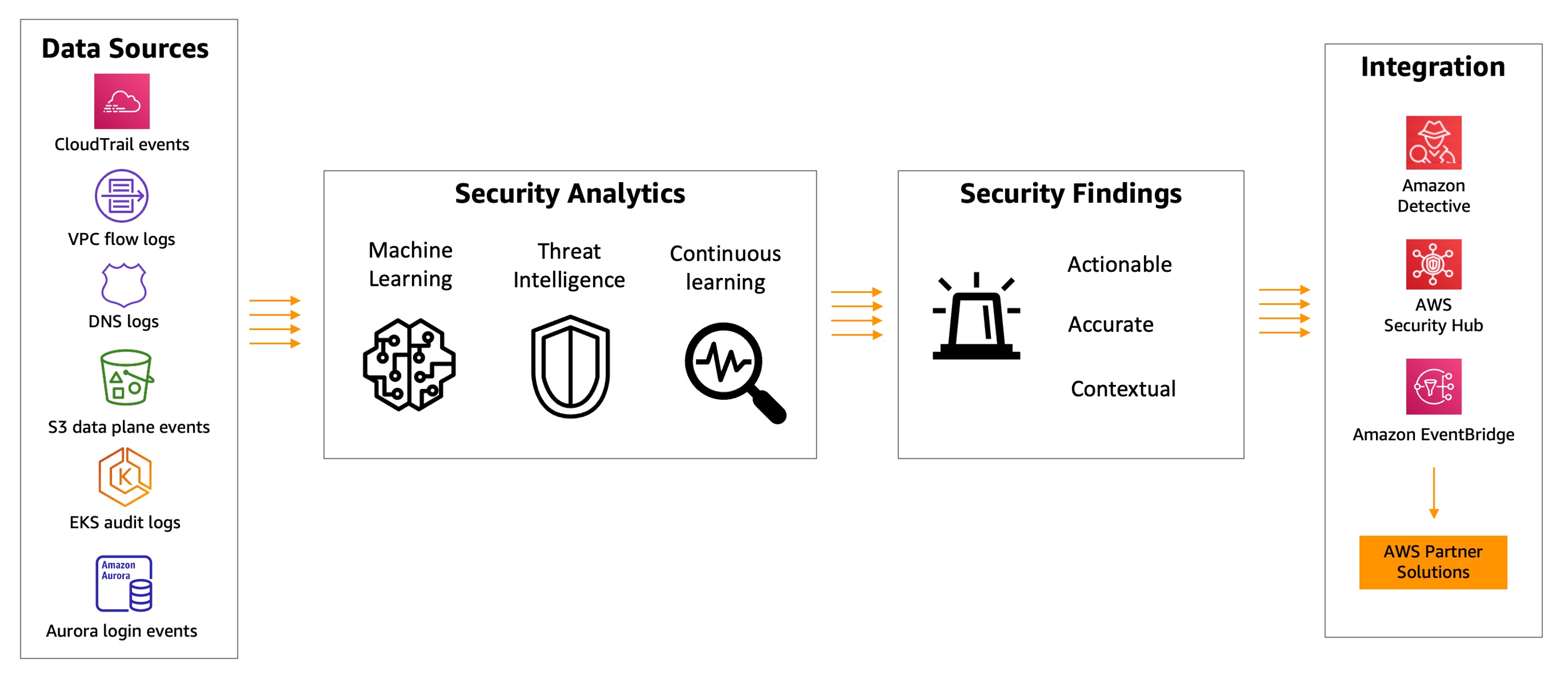

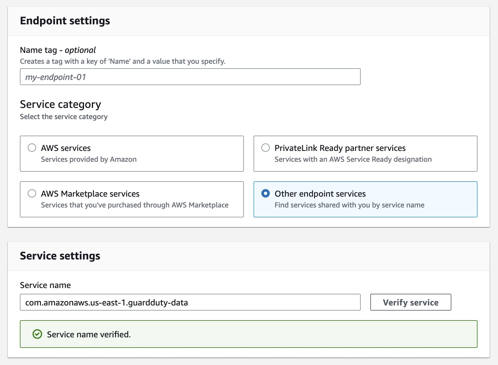
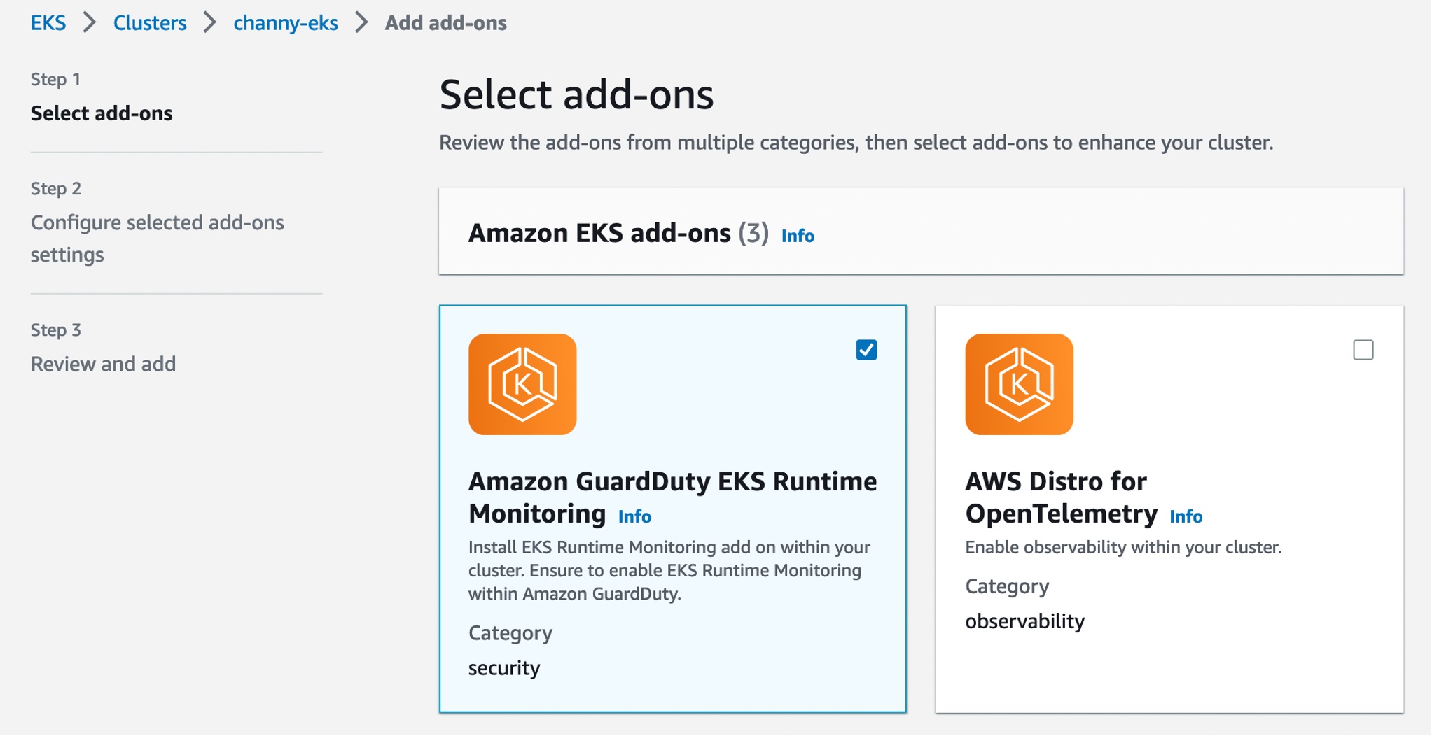


 Aruna Govindaraju is an Amazon OpenSearch Specialist Solutions Architect and has worked with many commercial and open-source search engines. She is passionate about search, relevancy, and user experience. Her expertise with correlating end-user signals with search engine behavior has helped many customers improve their search experience. Her favorite pastime is hiking the New England trails and mountains.

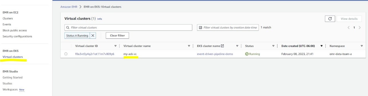

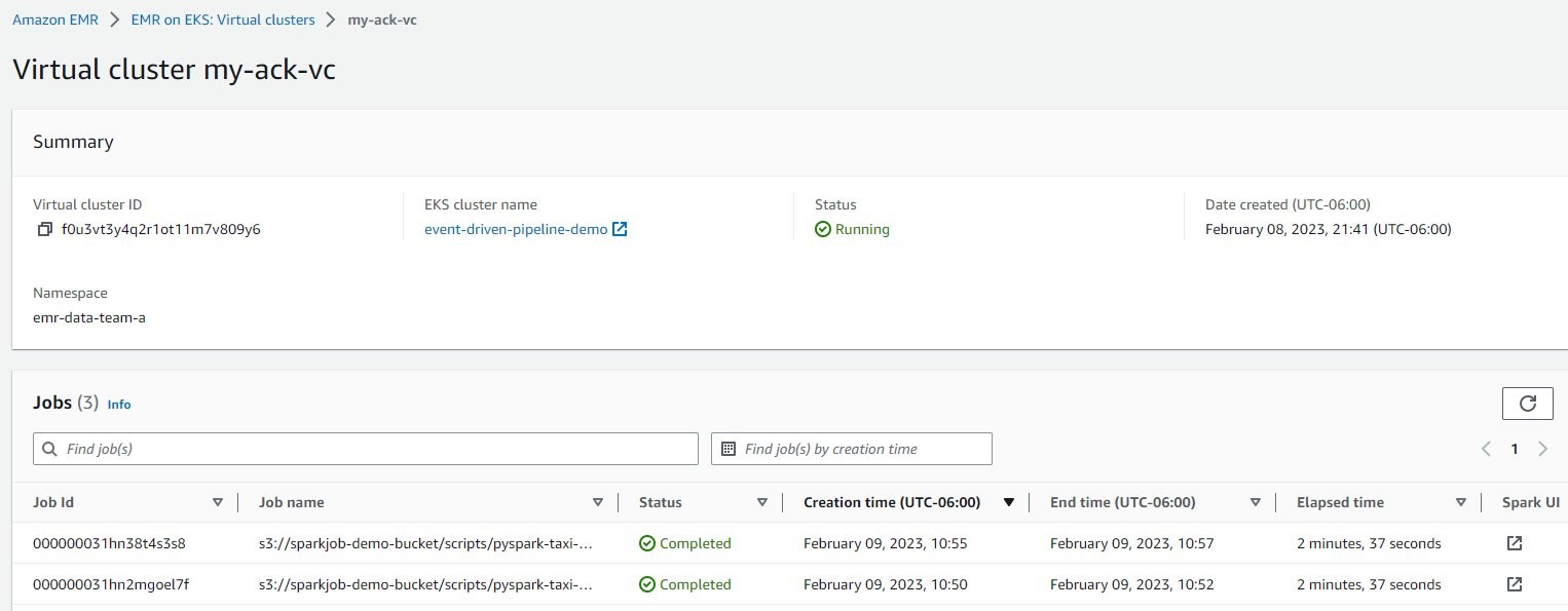
 Victor Gu is a Containers and Serverless Architect at AWS. He works with AWS customers to design microservices and cloud native solutions using Amazon EKS/ECS and AWS serverless services. His specialties are Kubernetes, Spark on Kubernetes, MLOps and DevOps.
 Michael Gasch is a Senior Product Manager for AWS EventBridge, driving innovations in event-driven architectures. Prior to AWS, Michael was a Staff Engineer at the VMware Office of the CTO, working on open-source projects, such as Kubernetes and Knative, and related distributed systems research.
 Peter Dalbhanjan is a Solutions Architect for AWS based in Herndon, VA. Peter has a keen interest in evangelizing AWS solutions and has written multiple blog posts that focus on simplifying complex use cases. At AWS, Peter helps with designing and architecting variety of customer workloads.