Post Syndicated from Luis Gerardo Baeza original https://aws.amazon.com/blogs/big-data/automate-replication-of-relational-sources-into-a-transactional-data-lake-with-apache-iceberg-and-aws-glue/
Organizations have chosen to build data lakes on top of Amazon Simple Storage Service (Amazon S3) for many years. A data lake is the most popular choice for organizations to store all their organizational data generated by different teams, across business domains, from all different formats, and even over history. According to a study, the average company is seeing the volume of their data growing at a rate that exceeds 50% per year, usually managing an average of 33 unique data sources for analysis.
Teams often try to replicate thousands of jobs from relational databases with the same extract, transform, and load (ETL) pattern. There is lot of effort in maintaining the job states and scheduling these individual jobs. This approach helps the teams add tables with few changes and also maintains the job status with minimum effort. This can lead to a huge improvement in the development timeline and tracking the jobs with ease.
In this post, we show you how to easily replicate all your relational data stores into a transactional data lake in an automated fashion with a single ETL job using Apache Iceberg and AWS Glue.
Solution architecture
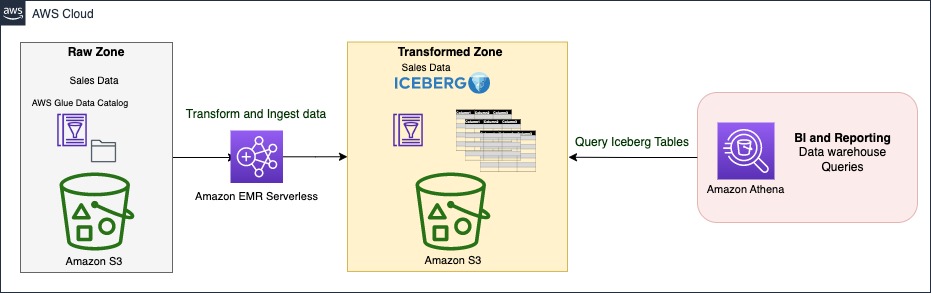
Data lakes are usually organized using separate S3 buckets for three layers of data: the raw layer containing data in its original form, the stage layer containing intermediate processed data optimized for consumption, and the analytics layer containing aggregated data for specific use cases. In the raw layer, tables usually are organized based on their data sources, whereas tables in the stage layer are organized based on the business domains they belong to.
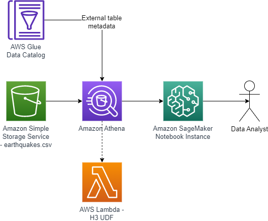
This post provides an AWS CloudFormation template that deploys an AWS Glue job that reads an Amazon S3 path for one data source of the data lake raw layer, and ingests the data into Apache Iceberg tables on the stage layer using AWS Glue support for data lake frameworks. The job expects tables in the raw layer to be structured in the way AWS Database Migration Service (AWS DMS) ingests them: schema, then table, then data files.
This solution uses AWS Systems Manager Parameter Store for table configuration. You should modify this parameter specifying the tables you want to process and how, including information such as primary key, partitions, and the business domain associated. The job uses this information to automatically create a database (if it doesn’t already exist) for every business domain, create the Iceberg tables, and perform the data loading.
Finally, we can use Amazon Athena to query the data in the Iceberg tables.
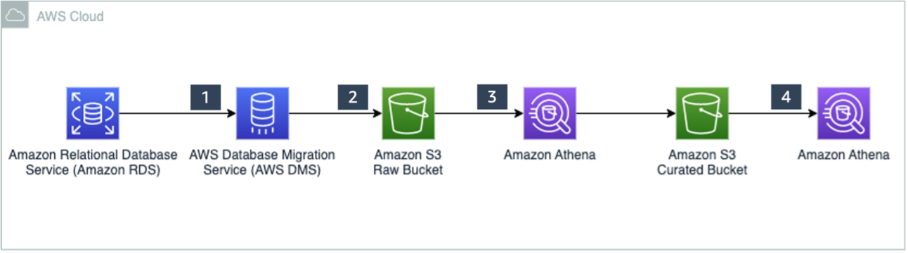
The following diagram illustrates this architecture.

This implementation has the following considerations:
- All tables from the data source must have a primary key to be replicated using this solution. The primary key can be a single column or a composite key with more than one column.
- If the data lake contains tables that don’t need upserts or don’t have a primary key, you can exclude them from the parameter configuration and implement traditional ETL processes to ingest them into the data lake. That’s outside of the scope of this post.
- If there are additional data sources that need to be ingested, you can deploy multiple CloudFormation stacks, one to handle each data source.
- The AWS Glue job is designed to process data in two phases: the initial load that runs after AWS DMS finishes the full load task, and the incremental load that runs on a schedule that applies change data capture (CDC) files captured by AWS DMS. Incremental processing is performed using an AWS Glue job bookmark.
There are nine steps to complete this tutorial:
- Set up a source endpoint for AWS DMS.
- Deploy the solution using AWS CloudFormation.
- Review the AWS DMS replication task.
- Optionally, add permissions for encryption and decryption or AWS Lake Formation.
- Review the table configuration on Parameter Store.
- Perform initial data loading.
- Perform incremental data loading.
- Monitor table ingestion.
- Schedule incremental batch data loading.
Prerequisites
Before starting this tutorial, you should already be familiar with Iceberg. If you’re not, you can get started by replicating a single table following the instructions in Implement a CDC-based UPSERT in a data lake using Apache Iceberg and AWS Glue. Additionally, set up the following:
Set up a source endpoint for AWS DMS
Before we create our AWS DMS task, we need to set up a source endpoint to connect to the source database:
- On the AWS DMS console, choose Endpoints in the navigation pane.
- Choose Create endpoint.
- If your database is running on Amazon RDS, choose Select RDS DB instance, then choose the instance from the list. Otherwise, choose the source engine and provide the connection information either through AWS Secrets Manager or manually.
- For Endpoint identifier, enter a name for the endpoint; for example, source-postgresql.
- Choose Create endpoint.
Deploy the solution using AWS CloudFormation
Create a CloudFormation stack using the provided template. Complete the following steps:
- Choose Launch Stack:

- Choose Next.
- Provide a stack name, such as
transactionaldl-postgresql.
- Enter the required parameters:
- DMSS3EndpointIAMRoleARN – The IAM role ARN for AWS DMS to write data into Amazon S3.
- ReplicationInstanceArn – The AWS DMS replication instance ARN.
- S3BucketStage – The name of the existing bucket used for the stage layer of the data lake.
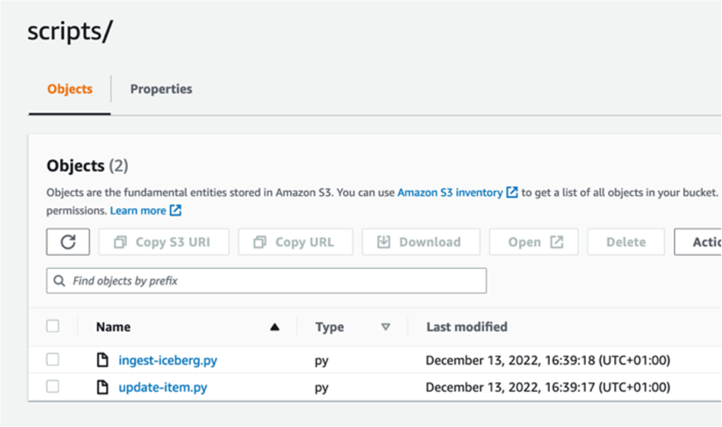
- S3BucketGlue – The name of the existing S3 bucket for storing AWS Glue scripts.
- S3BucketRaw – The name of the existing bucket used for the raw layer of the data lake.
- SourceEndpointArn – The AWS DMS endpoint ARN that you created earlier.
- SourceName – The arbitrary identifier of the data source to replicate (for example,
postgres). This is used to define the S3 path of the data lake (raw layer) where data will be stored.
- Do not modify the following parameters:
- SourceS3BucketBlog – The bucket name where the provided AWS Glue script is stored.
- SourceS3BucketPrefix – The bucket prefix name where the provided AWS Glue script is stored.
- Choose Next twice.
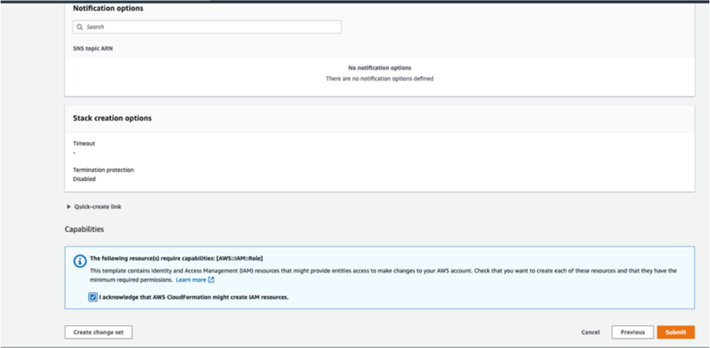
- Select I acknowledge that AWS CloudFormation might create IAM resources with custom names.
- Choose Create stack.
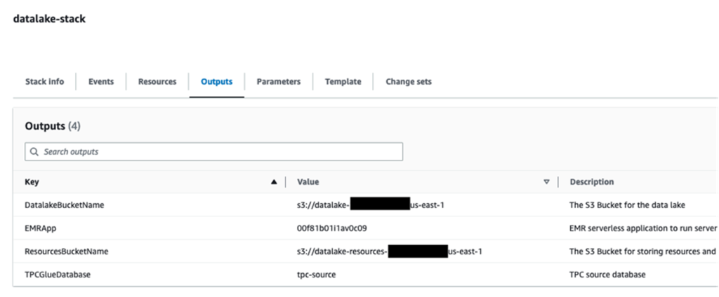
After approximately 5 minutes, the CloudFormation stack is deployed.
Review the AWS DMS replication task
The AWS CloudFormation deployment created an AWS DMS target endpoint for you. Because of two specific endpoint settings, the data will be ingested as we need it on Amazon S3.
- On the AWS DMS console, choose Endpoints in the navigation pane.
- Search for and choose the endpoint that begins with
dmsIcebergs3endpoint.
- Review the endpoint settings:
DataFormat is specified as parquet.TimestampColumnName will add the column last_update_time with the date of creation of the records on Amazon S3.

The deployment also creates an AWS DMS replication task that begins with dmsicebergtask.
- Choose Replication tasks in the navigation pane and search for the task.
You will see that the Task Type is marked as Full load, ongoing replication. AWS DMS will perform an initial full load of existing data, and then create incremental files with changes performed to the source database.
On the Mapping Rules tab, there are two types of rules:
- A selection rule with the name of the source schema and tables that will be ingested from the source database. By default, it uses the sample database provided in the prerequisites,
dms_sample, and all tables with the keyword %.
- Two transformation rules that include in the target files on Amazon S3 the schema name and table name as columns. This is used by our AWS Glue job to know to which tables the files in the data lake correspond.
To learn more about how to customize this for your own data sources, refer to Selection rules and actions.

Let’s change some configurations to finish our task preparation.
- On the Actions menu, choose Modify.
- In the Task Settings section, under Stop task after full load completes, choose Stop after applying cached changes.
This way, we can control the initial load and incremental file generation as two different steps. We use this two-step approach to run the AWS Glue job once per each step.
- Under Task logs, choose Turn on CloudWatch logs.
- Choose Save.
- Wait about 1 minute for the database migration task status to show as Ready.
Add permissions for encryption and decryption or Lake Formation
Optionally, you can add permissions for encryption and decryption or Lake Formation.
Add encryption and decryption permissions
If your S3 buckets used for the raw and stage layers are encrypted using AWS Key Management Service (AWS KMS) customer managed keys, you need to add permissions to allow the AWS Glue job to access the data:
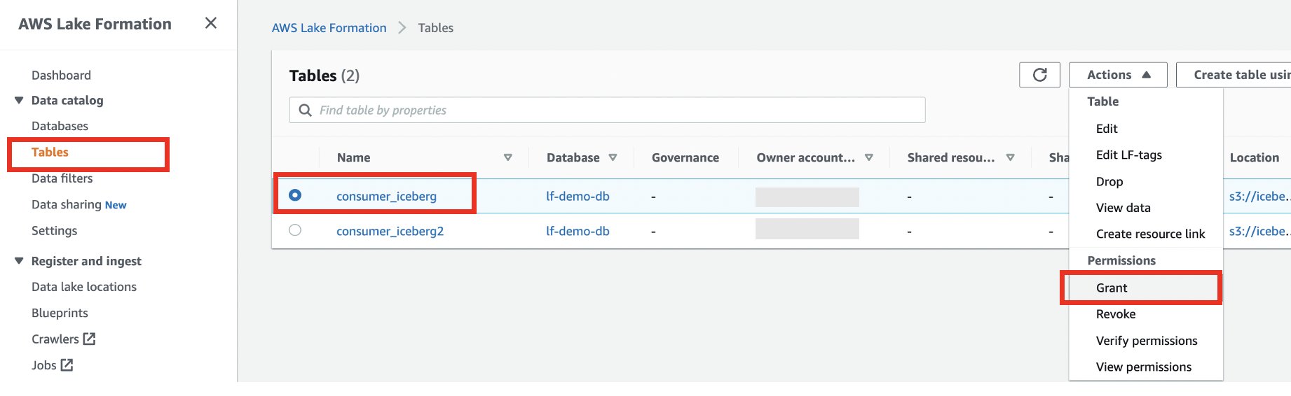
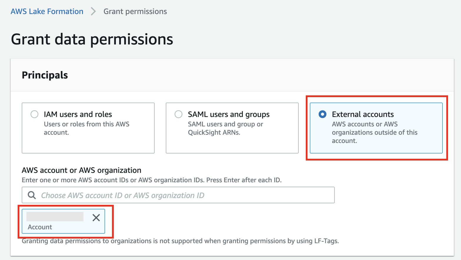
Add Lake Formation permissions
If you’re managing permissions using Lake Formation, you need to allow your AWS Glue job to create your domain’s databases and tables through the IAM role GlueJobRole.
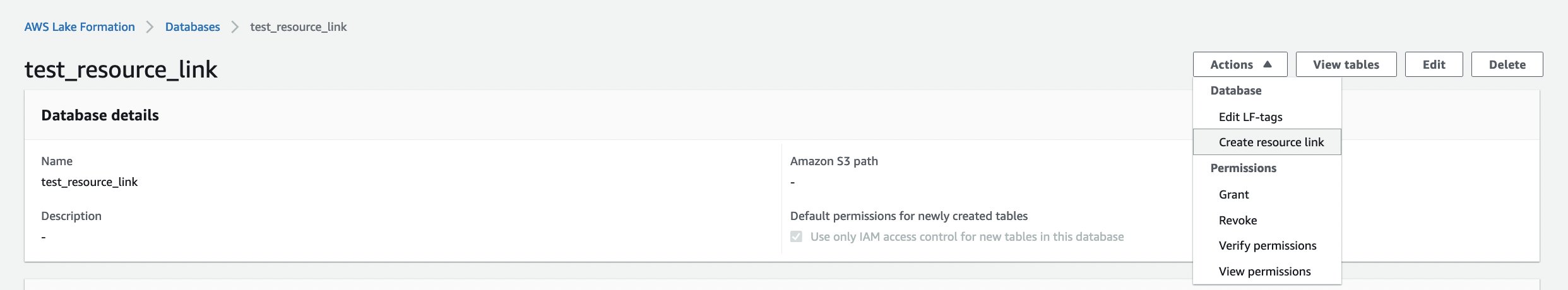
- Grant permissions to create databases (for instructions, refer to Creating a Database).
- Grant SUPER permissions to the
default database.
- Grant data location permissions.
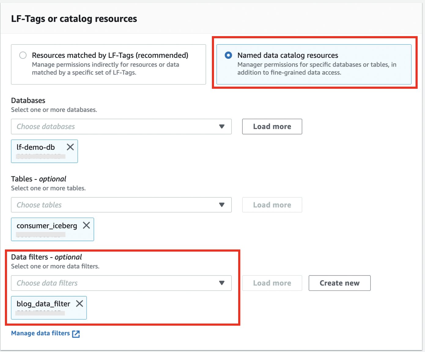
- If you create databases manually, grant permissions on all databases to create tables. Refer to Granting table permissions using the Lake Formation console and the named resource method or Granting Data Catalog permissions using the LF-TBAC method according to your use case.
After you complete the later step of performing the initial data load, make sure to also add permissions for consumers to query the tables. The job role will become the owner of all the tables created, and the data lake admin can then perform grants to additional users.
Review table configuration in Parameter Store
The AWS Glue job that performs the data ingestion into Iceberg tables uses the table specification provided in Parameter Store. Complete the following steps to review the parameter store that was configured automatically for you. If needed, modify according to your own needs.
- On the Parameter Store console, choose My parameters in the navigation pane.
The CloudFormation stack created two parameters:
iceberg-config for job configurationsiceberg-tables for table configuration
- Choose the parameter iceberg-tables.
The JSON structure contains information that AWS Glue uses to read data and write the Iceberg tables on the target domain:
- One object per table – The name of the object is created using the schema name, a period, and the table name; for example,
schema.table.
- primaryKey – This should be specified for every source table. You can provide a single column or a comma-separated list of columns (without spaces).
- partitionCols – This optionally partitions columns for target tables. If you don’t want to create partitioned tables, provide an empty string. Otherwise, provide a single column or a comma-separated list of columns to be used (without spaces).
- If you want to use your own data source, use the following JSON code and replace the text in CAPS from the template provided. If you’re using the sample data source provided, keep the default settings:
{
    "SCHEMA_NAME.TABLE_NAME_1": {
        "primaryKey": "ONLY_PRIMARY_KEY",
        "domain": "TARGET_DOMAIN",
        "partitionCols": ""
    },
    "SCHEMA_NAME.TABLE_NAME_2": {
        "primaryKey": "FIRST_PRIMARY_KEY,SECOND_PRIMARY_KEY",
        "domain": "TARGET_DOMAIN",
        "partitionCols": "PARTITION_COLUMN_ONE,PARTITION_COLUMN_TWO"
    }
}
- Choose Save changes.
Perform initial data loading
Now that the required configuration is finished, we ingest the initial data. This step includes three parts: ingesting the data from the source relational database into the raw layer of the data lake, creating the Iceberg tables on the stage layer of the data lake, and verifying results using Athena.
Ingest data into the raw layer of the data lake
To ingest data from the relational data source (PostgreSQL if you are using the sample provided) to our transactional data lake using Iceberg, complete the following steps:
- On the AWS DMS console, choose Database migration tasks in the navigation pane.
- Select the replication task you created and on the Actions menu, choose Restart/Resume.
- Wait about 5 minutes for the replication task to complete. You can monitor the tables ingested on the Statistics tab of the replication task.

After some minutes, the task finishes with the message Full load complete.
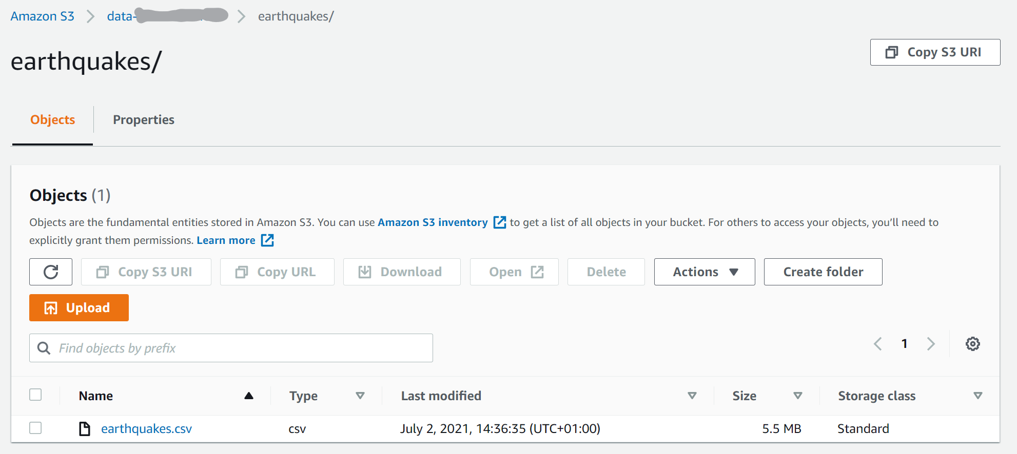
- On the Amazon S3 console, choose the bucket you defined as the raw layer.
Under the S3 prefix defined on AWS DMS (for example, postgres), you should see a hierarchy of folders with the following structure:
- Schema
- Table name
LOAD00000001.parquetLOAD0000000N.parquet

If your S3 bucket is empty, review Troubleshooting migration tasks in AWS Database Migration Service before running the AWS Glue job.
Create and ingest data into Iceberg tables
Before running the job, let’s navigate the script of the AWS Glue job provided as part of the CloudFormation stack to understand its behavior.
- On the AWS Glue Studio console, choose Jobs in the navigation pane.
- Search for the job that starts with
IcebergJob- and a suffix of your CloudFormation stack name (for example, IcebergJob-transactionaldl-postgresql).
- Choose the job.

The job script gets the configuration it needs from Parameter Store. The function getConfigFromSSM() returns job-related configurations such as source and target buckets from where the data needs to be read and written. The variable ssmparam_table_values contain table-related information like the data domain, table name, partition columns, and primary key of the tables that needs to be ingested. See the following Python code:
# Main application
args = getResolvedOptions(sys.argv, ['JOB_NAME', 'stackName'])
SSM_PARAMETER_NAME = f"{args['stackName']}-iceberg-config"
SSM_TABLE_PARAMETER_NAME = f"{args['stackName']}-iceberg-tables"

# Parameters for job
rawS3BucketName, rawBucketPrefix, stageS3BucketName, warehouse_path = getConfigFromSSM(SSM_PARAMETER_NAME)
ssm_param_table_values = json.loads(ssmClient.get_parameter(Name = SSM_TABLE_PARAMETER_NAME)['Parameter']['Value'])
dropColumnList = ['db','table_name', 'schema_name','Op', 'last_update_time', 'max_op_date']
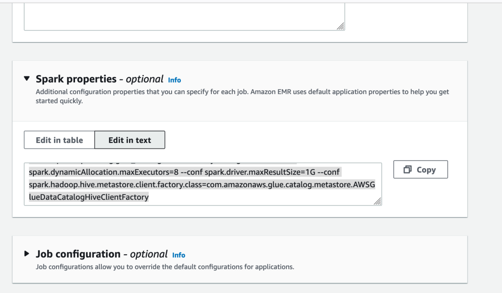
The script uses an arbitrary catalog name for Iceberg that is defined as my_catalog. This is implemented on the AWS Glue Data Catalog using Spark configurations, so a SQL operation pointing to my_catalog will be applied on the Data Catalog. See the following code:
catalog_name = 'my_catalog'
errored_table_list = []

# Iceberg configuration
spark = SparkSession.builder \
    .config('spark.sql.warehouse.dir', warehouse_path) \
    .config(f'spark.sql.catalog.{catalog_name}', 'org.apache.iceberg.spark.SparkCatalog') \
    .config(f'spark.sql.catalog.{catalog_name}.warehouse', warehouse_path) \
    .config(f'spark.sql.catalog.{catalog_name}.catalog-impl', 'org.apache.iceberg.aws.glue.GlueCatalog') \
    .config(f'spark.sql.catalog.{catalog_name}.io-impl', 'org.apache.iceberg.aws.s3.S3FileIO') \
    .config('spark.sql.extensions', 'org.apache.iceberg.spark.extensions.IcebergSparkSessionExtensions') \
    .getOrCreate()
The script iterates over the tables defined in Parameter Store and performs the logic for detecting if the table exists and if the incoming data is an initial load or an upsert:
# Iteration over tables stored on Parameter Store
for key in ssm_param_table_values:
    # Get table data
    isTableExists = False
    schemaName, tableName = key.split('.')
    logger.info(f'Processing table : {tableName}')
The initialLoadRecordsSparkSQL() function loads initial data when no operation column is present in the S3 files. AWS DMS adds this column only to Parquet data files produced by the continuous replication (CDC). The data loading is performed using the INSERT INTO command with SparkSQL. See the following code:
sqltemp = Template("""
    INSERT INTO $catalog_name.$dbName.$tableName  ($insertTableColumnList)
    SELECT $insertTableColumnList FROM insertTable $partitionStrSQL
""")
SQLQUERY = sqltemp.substitute(
    catalog_name = catalog_name,
    dbName = dbName,
    tableName = tableName,
    insertTableColumnList = insertTableColumnList[ : -1],
    partitionStrSQL = partitionStrSQL)

logger.info(f'****SQL QUERY IS : {SQLQUERY}')
spark.sql(SQLQUERY)
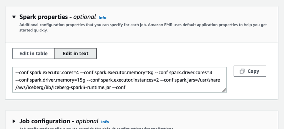
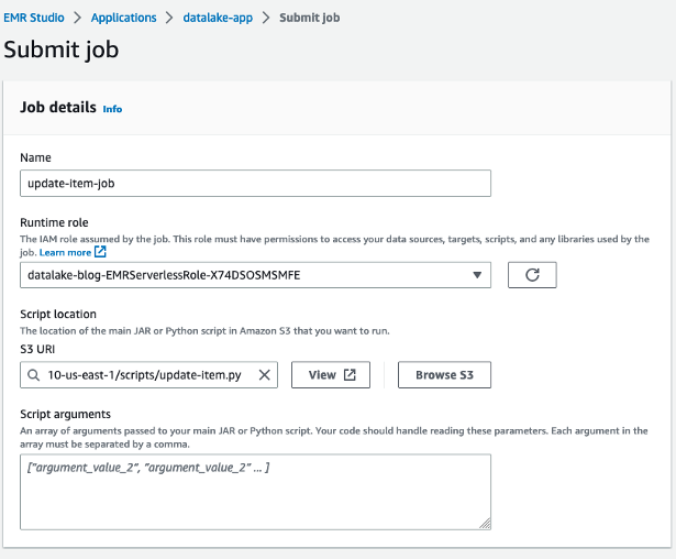
Now we run the AWS Glue job to ingest the initial data into the Iceberg tables. The CloudFormation stack adds the --datalake-formats parameter, adding the required Iceberg libraries to the job.
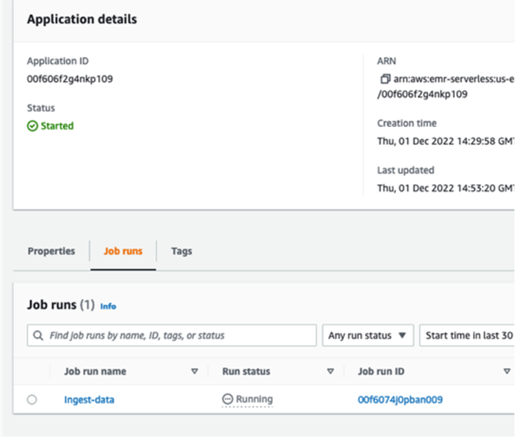
- Choose Run job.
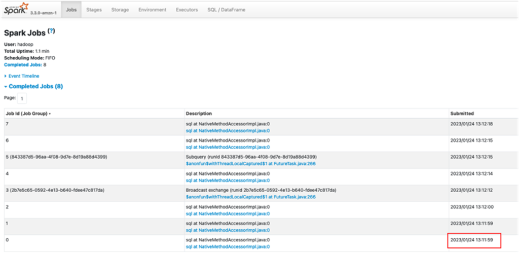
- Choose Job Runs to monitor the status. Wait until the status is Run Succeeded.
Verify the data loaded
To confirm that the job processed the data as expected, complete the following steps:
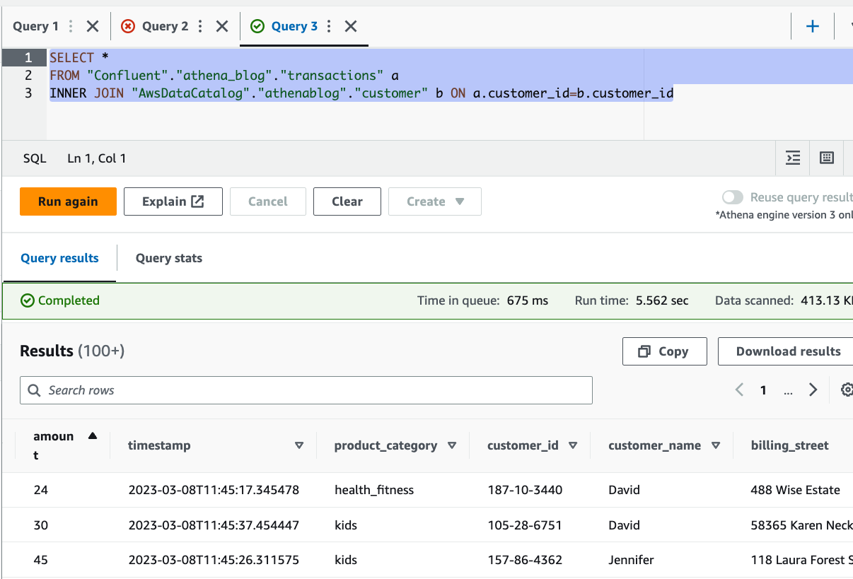
- On the Athena console, choose Query Editor in the navigation pane.
- Verify
AwsDataCatalog is selected as the data source.
- Under Database, choose the data domain that you want to explore, based on the configuration you defined in the parameter store. If using the sample database provided, use
sports.
Under Tables and views, we can see the list of tables that were created by the AWS Glue job.
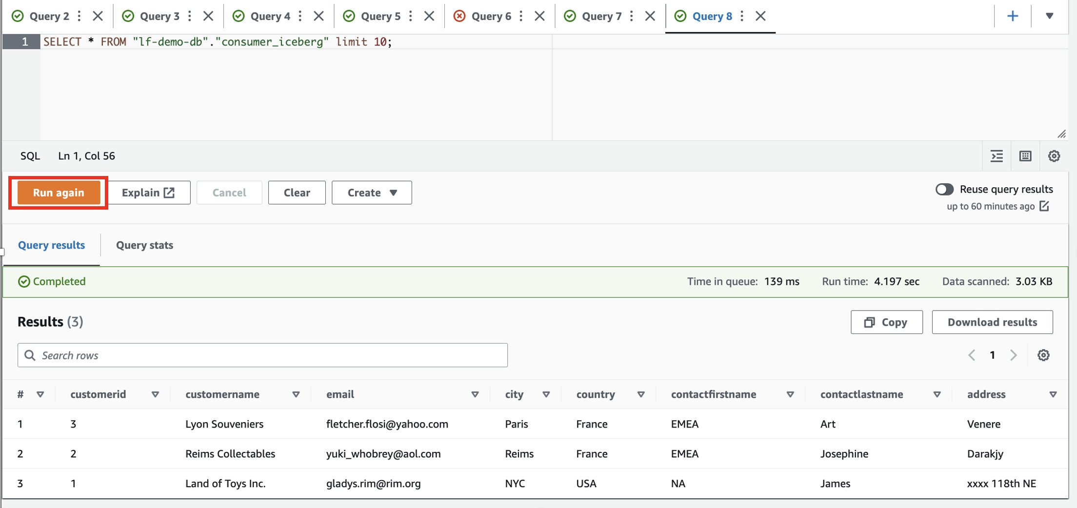
- Choose the options menu (three dots) next to the first table name, then choose Preview Data.
You can see the data loaded into Iceberg tables. 
Perform incremental data loading
Now we start capturing changes from our relational database and applying them to the transactional data lake. This step is also divided in three parts: capturing the changes, applying them to the Iceberg tables, and verifying the results.
Capture changes from the relational database
Due to the configuration we specified, the replication task stopped after running the full load phase. Now we restart the task to add incremental files with changes into the raw layer of the data lake.
- On the AWS DMS console, select the task we created and ran before.
- On the Actions menu, choose Resume.
- Choose Start task to start capturing changes.
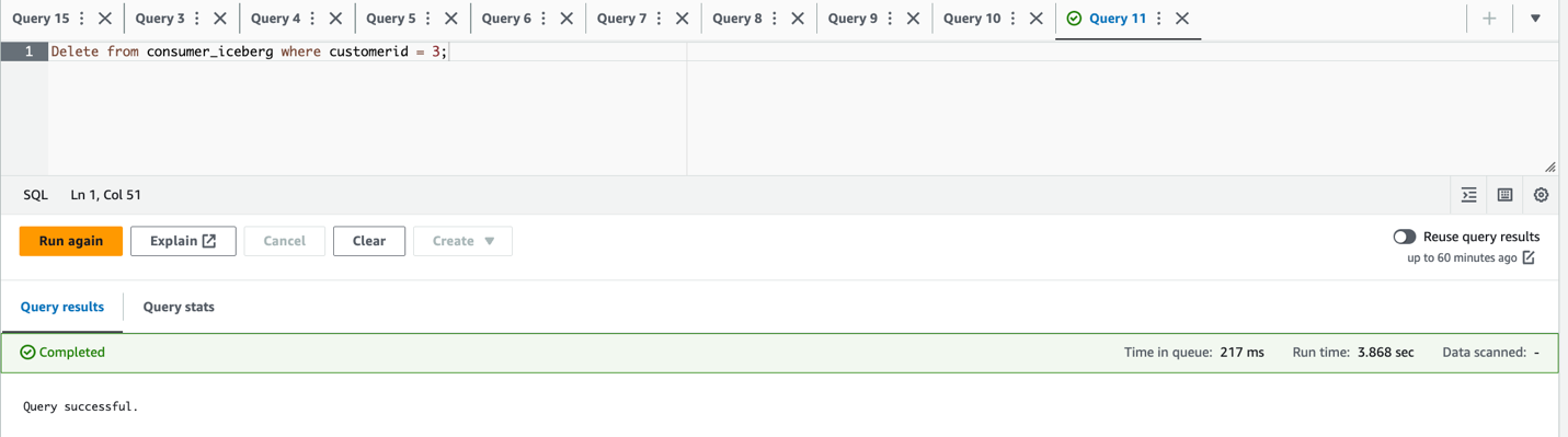
- To trigger new file creation on the data lake, perform inserts, updates, or deletes on the tables of your source database using your preferred database administration tool. If using the sample database provided, you could run the following SQL commands:
UPDATE dms_sample.nfl_stadium_data_upd
SET seatin_capacity=93703
WHERE team = 'Los Angeles Rams' and sport_location_id = '31';

update  dms_sample.mlb_data
set bats = 'R'
where mlb_id=506560 and bats='L';

update dms_sample.sporting_event
set start_date  = current_date
where id=11 and sold_out=0;
- On the AWS DMS task details page, choose the Table statistics tab to see the changes captured.

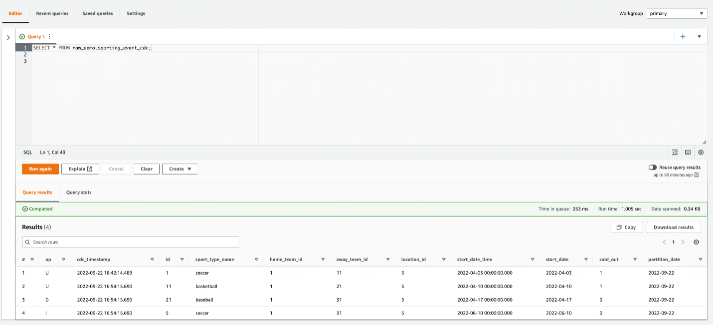
- Open the raw layer of the data lake to find a new file holding the incremental changes inside every table’s prefix, for example under the
sporting_event prefix.
The record with changes for the sporting_event table looks like the following screenshot.

Notice the Op column in the beginning identified with an update (U). Also, the second date/time value is the control column added by AWS DMS with the time the change was captured.

Apply changes on the Iceberg tables using AWS Glue
Now we run the AWS Glue job again, and it will automatically process only the new incremental files since the job bookmark is enabled. Let’s review how it works.
The dedupCDCRecords() function performs deduplication of data because multiple changes to a single record ID could be captured within the same data file on Amazon S3. Deduplication is performed based on the last_update_time column added by AWS DMS that indicates the timestamp of when the change was captured. See the following Python code:
def dedupCDCRecords(inputDf, keylist):
    IDWindowDF = Window.partitionBy(*keylist).orderBy(inputDf.last_update_time).rangeBetween(-sys.maxsize, sys.maxsize)
    inputDFWithTS = inputDf.withColumn('max_op_date', max(inputDf.last_update_time).over(IDWindowDF))

    NewInsertsDF = inputDFWithTS.filter('last_update_time=max_op_date').filter("op='I'")
    UpdateDeleteDf = inputDFWithTS.filter('last_update_time=max_op_date').filter("op IN ('U','D')")
    finalInputDF = NewInsertsDF.unionAll(UpdateDeleteDf)

    return finalInputDF
On line 99, the upsertRecordsSparkSQL() function performs the upsert in a similar fashion to the initial load, but this time with a SQL MERGE command.
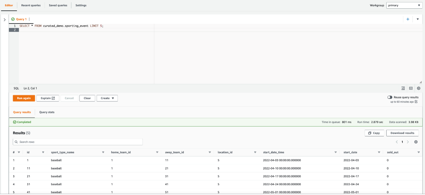
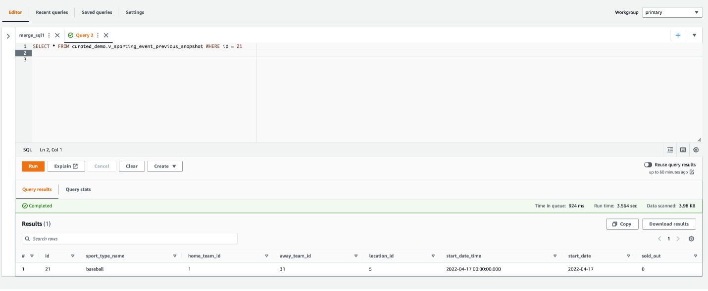
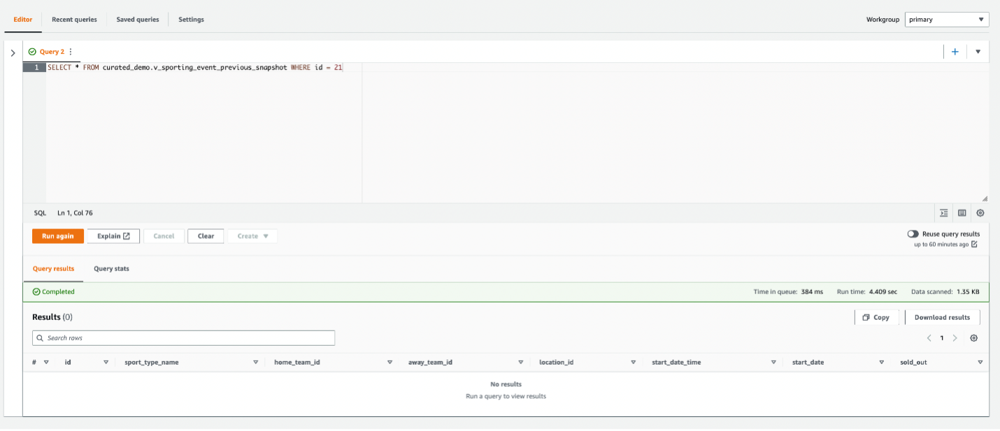
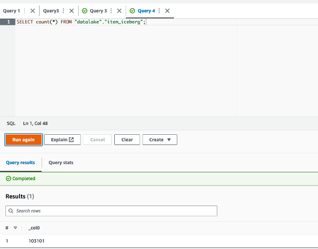
Review the applied changes
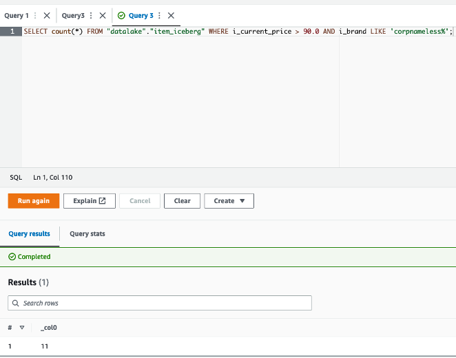
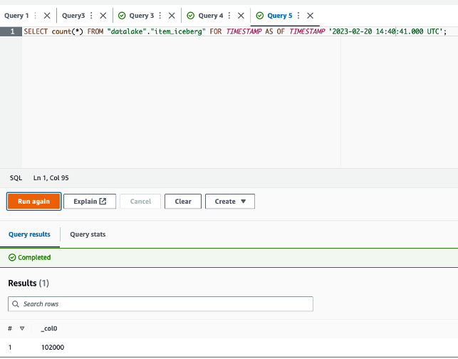
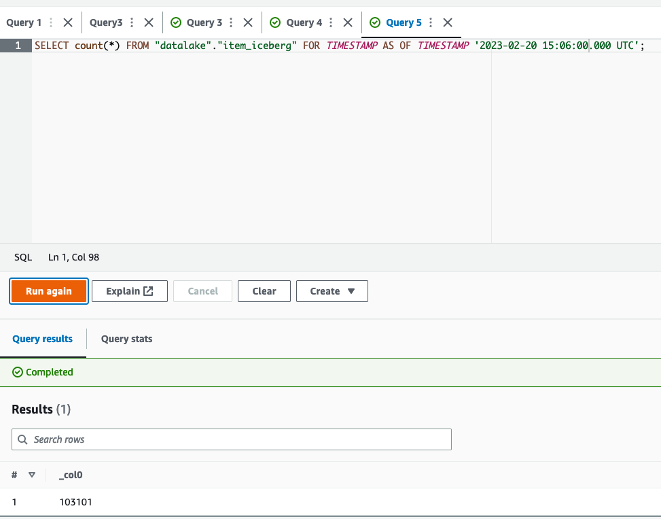
Open the Athena console and run a query that selects the changed records on the source database. If using the provided sample database, use one the following SQL queries:
SELECT * FROM "sports"."nfl_stadiu_data_upd"
WHERE team = 'Los Angeles Rams' and sport_location_id = 31
LIMIT 1;

Monitor table ingestion
The AWS Glue job script is coded with simple Python exception handling to catch errors during processing a specific table. The job bookmark is saved after each table finishes processing successfully, to avoid reprocessing tables if the job run is retried for the tables with errors.
The AWS Command Line Interface (AWS CLI) provides a get-job-bookmark command for AWS Glue that provides insight into the status of the bookmark for each table processed.
- On the AWS Glue Studio console, choose the ETL job.
- Choose the Job Runs tab and copy the job run ID.
- Run the following command on a terminal authenticated for the AWS CLI, replacing
<GLUE_JOB_RUN_ID> on line 1 with the value you copied. If your CloudFormation stack is not named transactionaldl-postgresql, provide the name of your job on line 2 of the script:
jobrun=<GLUE_JOB_RUN_ID>
jobname=IcebergJob-transactionaldl-postgresql
aws glue get-job-bookmark --job-name jobname --run-id $jobrun
In this solution, when a table processing causes an exception, the AWS Glue job will not fail according to this logic. Instead, the table will be added into an array that is printed after the job is complete. In such scenario, the job will be marked as failed after it tries to process the rest of the tables detected on the raw data source. This way, tables without errors don’t have to wait until the user identifies and solves the problem on the conflicting tables. The user can quickly detect job runs that had issues using the AWS Glue job run status, and identify which specific tables are causing the problem using the CloudWatch logs for the job run.
- The job script implements this feature with the following Python code:
# Performed for every table
        try:
            # Table processing logic
        except Exception as e:
            logger.info(f'There is an issue with table: {tableName}')
            logger.info(f'The exception is : {e}')
            errored_table_list.append(tableName)
            continue
        job.commit()
if (len(errored_table_list)):
    logger.info('Total number of errored tables are ',len(errored_table_list))
    logger.info('Tables that failed during processing are ', *errored_table_list, sep=', ')
    raise Exception(f'***** Some tables failed to process.')
The following screenshot shows how the CloudWatch logs look for tables that cause errors on processing.

Aligned with the AWS Well-Architected Framework Data Analytics Lens practices, you can adapt more sophisticated control mechanisms to identify and notify stakeholders when errors appear on the data pipelines. For example, you can use an Amazon DynamoDB control table to store all tables and job runs with errors, or using Amazon Simple Notification Service (Amazon SNS) to send alerts to operators when certain criteria is met.
Schedule incremental batch data loading
The CloudFormation stack deploys an Amazon EventBridge rule (disabled by default) that can trigger the AWS Glue job to run on a schedule. To provide your own schedule and enable the rule, complete the following steps:
- On the EventBridge console, choose Rules in the navigation pane.
- Search for the rule prefixed with the name of your CloudFormation stack followed by
JobTrigger (for example, transactionaldl-postgresql-JobTrigger-randomvalue).
- Choose the rule.
- Under Event Schedule, choose Edit.
The default schedule is configured to trigger every hour.
- Provide the schedule you want to run the job.
- Additionally, you can use an EventBridge cron expression by selecting A fine-grained schedule.

- When you finish setting up the cron expression, choose Next three times, and finally choose Update Rule to save changes.
The rule is created disabled by default to allow you to run the initial data load first.
- Activate the rule by choosing Enable.
You can use the Monitoring tab to view rule invocations, or directly on the AWS Glue Job Run details.
Conclusion
After deploying this solution, you have automated the ingestion of your tables on a single relational data source. Organizations using a data lake as their central data platform usually need to handle multiple, sometimes even tens of data sources. Also, more and more use cases require organizations to implement transactional capabilities to the data lake. You can use this solution to accelerate the adoption of such capabilities across all your relational data sources to enable new business use cases, automating the implementation process to derive more value from your data.
About the Authors
 Luis Gerardo Baeza is a Big Data Architect in the Amazon Web Services (AWS) Data Lab. He has 12 years of experience helping organizations in the healthcare, financial and education sectors to adopt enterprise architecture programs, cloud computing, and data analytics capabilities. Luis currently helps organizations across Latin America to accelerate strategic data initiatives.
 SaiKiran Reddy Aenugu is a Data Architect in the Amazon Web Services (AWS) Data Lab. He has 10 years of experience implementing data loading, transformation, and visualization processes. SaiKiran currently helps organizations in North America to adopt modern data architectures such as data lakes and data mesh. He has experience in the retail, airline, and finance sectors.
 Narendra Merla is a Data Architect in the Amazon Web Services (AWS) Data Lab. He has 12 years of experience in designing and productionalizing both real-time and batch-oriented data pipelines and building data lakes on both cloud and on-premises environments. Narendra currently helps organizations in North America to build and design robust data architectures, and has experience in the telecom and finance sectors.


 Sumesh M R is a Full Stack Machine Learning Architect at Cargotec. He has several years of software engineering and ML background. Sumesh is an expert in Sagemaker and other AWS ML/Analytics services. He is passionate about data science and loves to explore the latest ML libraries and techniques. Before joining Cargotec, he worked as a Solution Architect at TCS. In his spare time, he loves to play cricket and badminton.
 Tero Karttunen is a Senior Cloud Architect at Knowit Finland. He advises clients on architecting and adopting Data Architectures that best serve their Data Analytics and Machine Learning needs. He has helped Cargotec in their data journey for more than two years. Outside of work, he enjoys running, winter sports, and role-playing games.
 Arun A K is a Big Data Specialist Solutions Architect at AWS. He works with customers to provide architectural guidance for running analytics solutions on AWS Glue, AWS Lake Formation, Amazon Athena, and Amazon EMR. In his free time, he likes to spend time with his friends and family.


 Jonatan Selsing is former research scientist with a PhD in astrophysics that has turned to the cloud. He is currently the Lead Cloud Engineer at Novo Nordisk, where he enables data and analytics workloads at scale. With an emphasis on reducing the total cost of ownership of cloud-based workloads, while giving full benefit of the advantages of cloud, he designs, builds, and maintains solutions that enable research for future medicines.
 Hassen Riahi is a Sr. Data Architect at AWS Professional Services. He holds a PhD in Mathematics & Computer Science on large-scale data management. He works with AWS customers on building data-driven solutions.
 Alessandro Fior is a Sr. Data Architect at AWS Professional Services. He is passionate about designing and building modern and scalable data platforms that accelerate companies to extract value from their data.


 Ranjit Rajan is a Principal Data Lab Solutions Architect with AWS. Ranjit works with AWS customers to help them design and build data and analytics applications in the cloud.
 Kannan Iyer is a Senior Data Lab Solutions Architect with AWS. Kannan works with AWS customers to help them design and build data and analytics applications in the cloud.
 Alexandre Rezende is a Data Lab Solutions Architect with AWS. Alexandre works with customers on their Business Intelligence, Data Warehouse, and Data Lake use cases, design architectures to solve their business problems, and helps them build MVPs to accelerate their path to production.
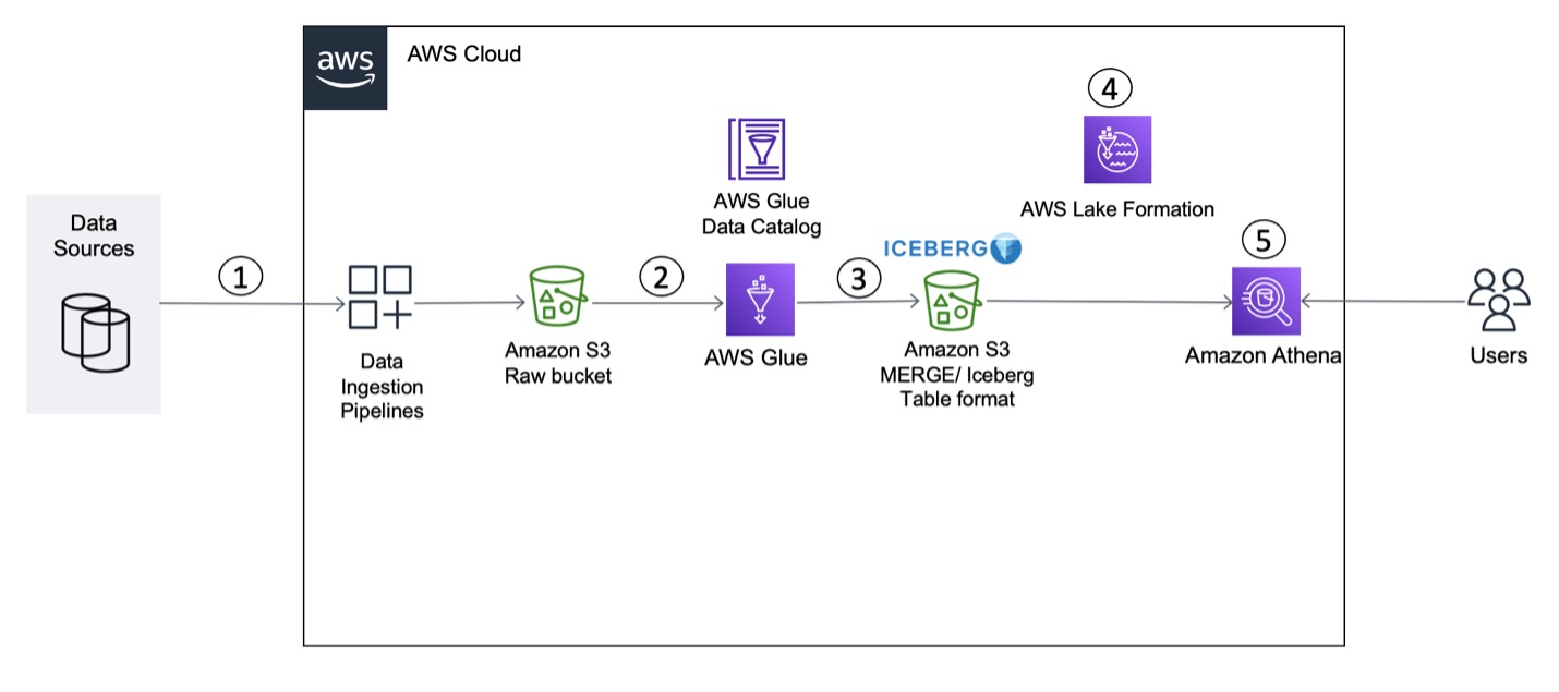


 Vikram Sahadevan is a Senior Resident Architect on the AWS Data Lab team. He enjoys efforts that focus around providing prescriptive architectural guidance, sharing best practices, and removing technical roadblocks with joint engineering engagements between customers and AWS technical resources that accelerate data, analytics, artificial intelligence, and machine learning initiatives.
 Suvendu Kumar Patra possesses 18 years of experience in infrastructure, database design, and data engineering, and he currently holds the position of Senior Resident Architect at Amazon Web Services. He is a member of the specialized focus group, AWS Data Lab, and his primary duties entail working with executive leadership teams of strategic AWS customers to develop their roadmaps for data, analytics, and AI/ML. Suvendu collaborates closely with customers to implement data engineering, data hub, data lake, data governance, and EDW solutions, as well as enterprise data strategy and data management.


 Ahmed Zamzam is a Senior Partner Solutions Architect at Confluent, with a focus on the AWS partnership. In his role, he works with customers in the EMEA region across various industries to assist them in building applications that leverage their data using Confluent and AWS. Prior to Confluent, Ahmed was a Specialist Solutions Architect for Analytics AWS specialized in data streaming and search. In his free time, Ahmed enjoys traveling, playing tennis, and cycling.
 Geetha Anne is a Partner Solutions Engineer at Confluent with previous experience in implementing solutions for data-driven business problems on the cloud, involving data warehousing and real-time streaming analytics. She fell in love with distributed computing during her undergraduate days and has followed her interest ever since. Geetha provides technical guidance, design advice, and thought leadership to key Confluent customers and partners. She also enjoys teaching complex technical concepts to both tech-savvy and general audiences.


 Chris Olson is a Software Development Engineer at AWS.
 Xiaoxuan Li is a Software Development Engineer at AWS.


 John Telford is a Senior Consultant at Amazon Web Services. He is a specialist in big data and data warehouses. John has a Computer Science degree from Brunel University.
 Pauline Ting is a Data Scientist in the AWS Professional Services team. She supports customers in achieving and accelerating their business outcome by developing sustainable AI/ML solutions. In her spare time, Pauline enjoys traveling, surfing, and trying new dessert places.
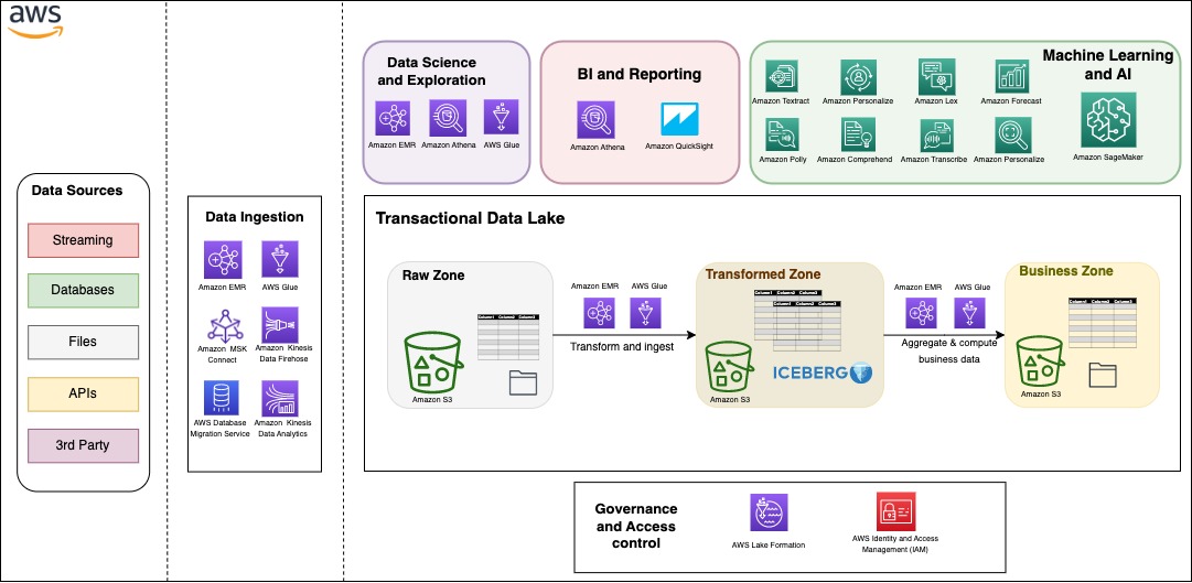

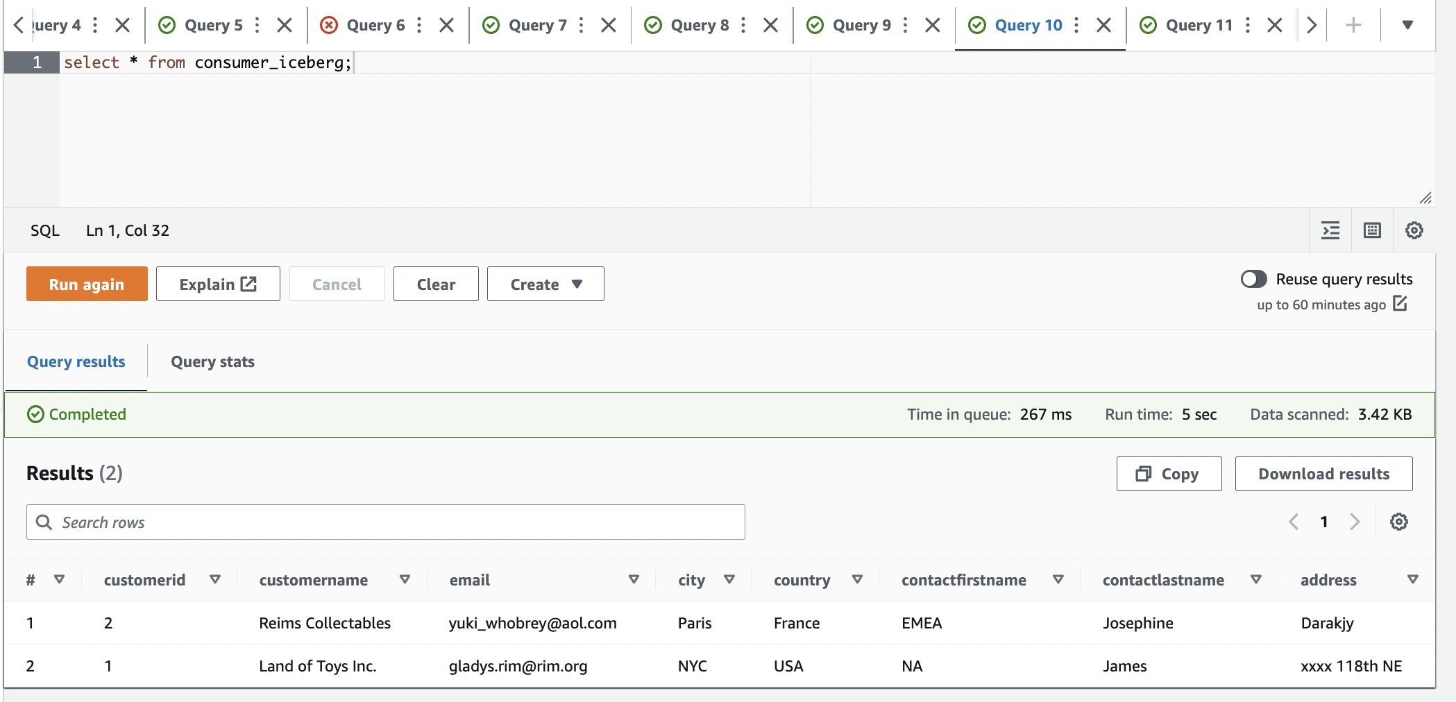
 The queries in
 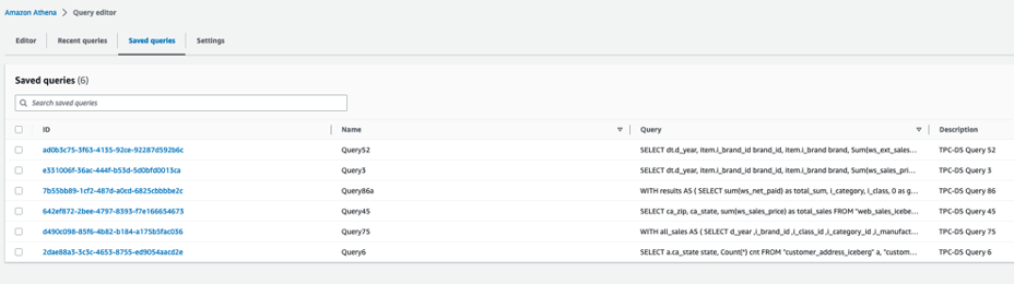 The following queries are listed:


 Naresh Gautam is a Data Analytics and AI/ML leader at AWS with 20 years of experience, who enjoys helping customers architect highly available, high-performance, and cost-effective data analytics and AI/ML solutions to empower customers with data-driven decision-making. In his free time, he enjoys meditation and cooking.
 Srikanth Sopirala is a Principal Analytics Specialist Solutions Architect at AWS. He is a seasoned leader with over 20 years of experience, who is passionate about helping customers build scalable data and analytics solutions to gain timely insights and make critical business decisions. In his spare time, he enjoys reading, spending time with his family, and road biking.
 Harsh Vardhan is an AWS Solutions Architect, specializing in analytics. He has over 5 years of experience working in the field of big data and data science. He is passionate about helping customers adopt best practices and discover insights from their data.
 Abhi Sodhani is a Sr. AI/ML Solutions Architect at AWS. He helps customers with a wide range of solutions, including machine leaning, artificial intelligence, data lakes, data warehousing, and data visualization. Outside of work, he is passionate about books, yoga, and travel.


 Flora Wu is a Sr. Resident Architect at AWS Data Lab. She helps enterprise customers create data analytics strategies and build solutions to accelerate their businesses outcomes. In her spare time, she enjoys playing tennis, dancing salsa, and traveling.
 Daniel Li is a Sr. Solutions Architect at Amazon Web Services. He focuses on helping customers develop, adopt, and implement cloud services and strategy. When not working, he likes spending time outdoors with his family.
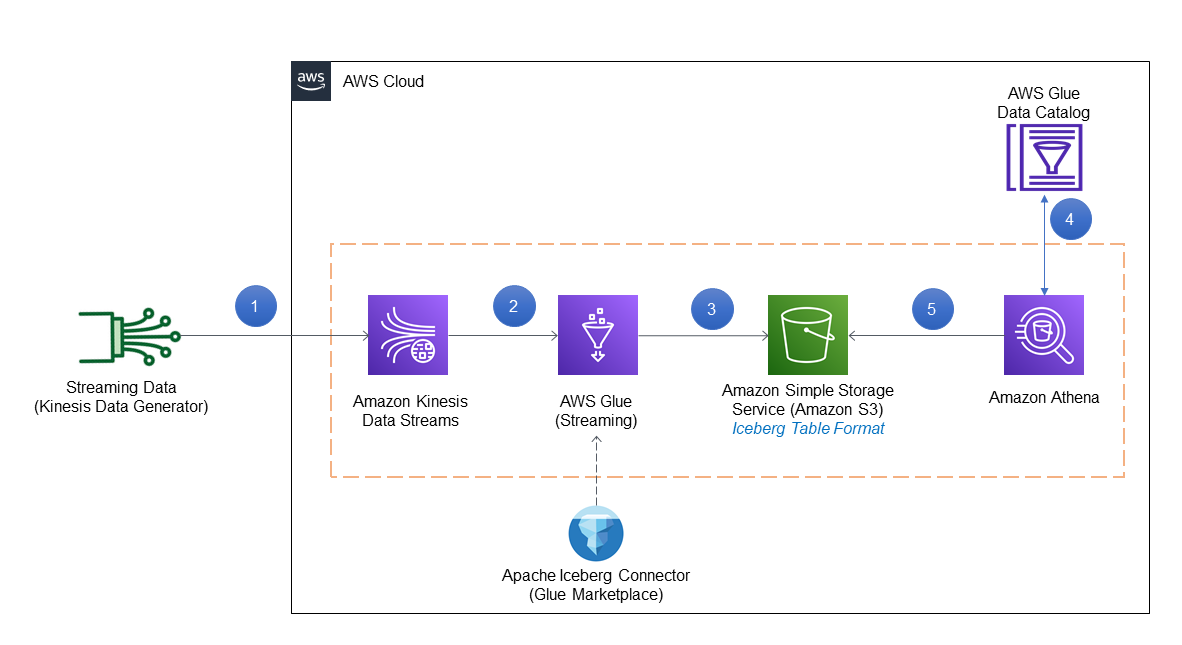


 Dhiraj Thakur is a Solutions Architect with Amazon Web Services. He works with AWS customers and partners to provide guidance on enterprise cloud adoption, migration, and strategy. He is passionate about technology and enjoys building and experimenting in the analytics and AI/ML space.
 Rajdip Chaudhuri is Solutions Architect with Amazon Web Services specializing in data and analytics. He enjoys working with AWS customers and partners on data and analytics requirements. In his spare time, he enjoys soccer.


 SaiKiran Reddy Aenugu is a Data Architect in the Amazon Web Services (AWS) Data Lab. He has 10 years of experience implementing data loading, transformation, and visualization processes. SaiKiran currently helps organizations in North America to adopt modern data architectures such as data lakes and data mesh. He has experience in the retail, airline, and finance sectors.
 Narendra Merla is a Data Architect in the Amazon Web Services (AWS) Data Lab. He has 12 years of experience in designing and productionalizing both real-time and batch-oriented data pipelines and building data lakes on both cloud and on-premises environments. Narendra currently helps organizations in North America to build and design robust data architectures, and has experience in the telecom and finance sectors.


 Avinash Kolluri is a Senior Solutions Architect at AWS. He works across Amazon Alexa and Devices to architect and design modern distributed solutions. His passion is to build cost-effective and highly scalable solutions on AWS. In his spare time, he enjoys cooking fusion recipes and traveling.
 Vipul Verma is a Sr.Software Engineer at Amazon.com. He has been with Amazon since 2015,solving real-world challenges through technology that directly impact and improve the life of Amazon customers. In his spare time, he enjoys hiking.