Post Syndicated from Praveen Allam original https://aws.amazon.com/blogs/big-data/handle-upsert-data-operations-using-open-source-delta-lake-and-aws-glue/
Many customers need an ACID transaction (atomic, consistent, isolated, durable) data lake that can log change data capture (CDC) from operational data sources. There is also demand for merging real-time data into batch data. Delta Lake framework provides these two capabilities. In this post, we discuss how to handle UPSERTs (updates and inserts) of the operational data using natively integrated Delta Lake with AWS Glue, and query the Delta Lake using Amazon Athena.
We examine a hypothetical insurance organization that issues commercial policies to small- and medium-scale businesses. The insurance prices vary based on several criteria, such as where the business is located, business type, earthquake or flood coverage, and so on. This organization is planning to build a data analytical platform, and the insurance policy data is one of the inputs to this platform. Because the business is growing, hundreds and thousands of new insurance policies are being enrolled and renewed every month. Therefore, all this operational data needs to be sent to Delta Lake in near-real time so that the organization can perform various analytics, and build machine learning (ML) models to serve their customers in a more efficient and cost-effective way.
Solution overview
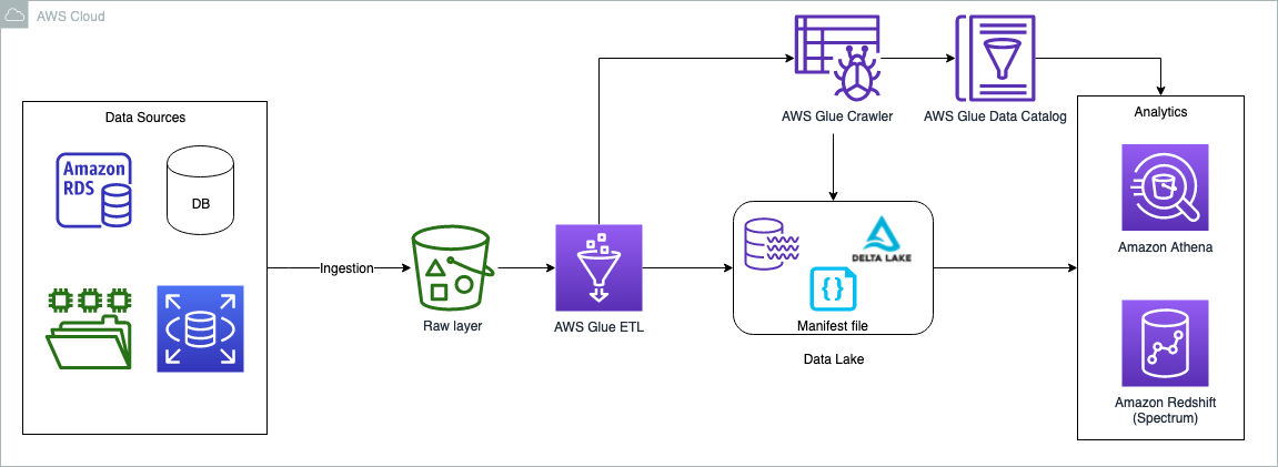
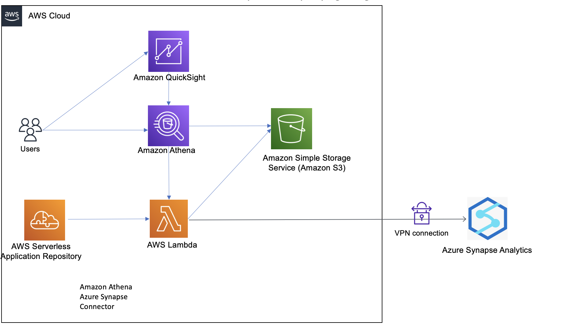
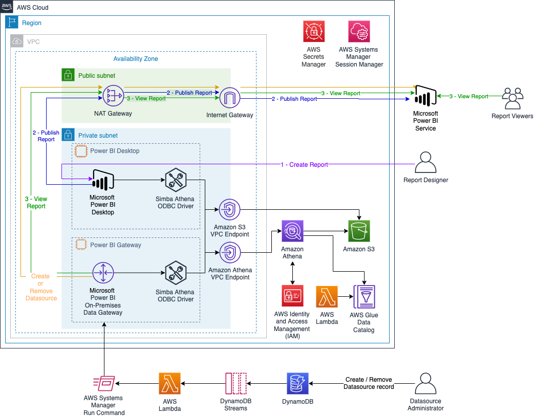
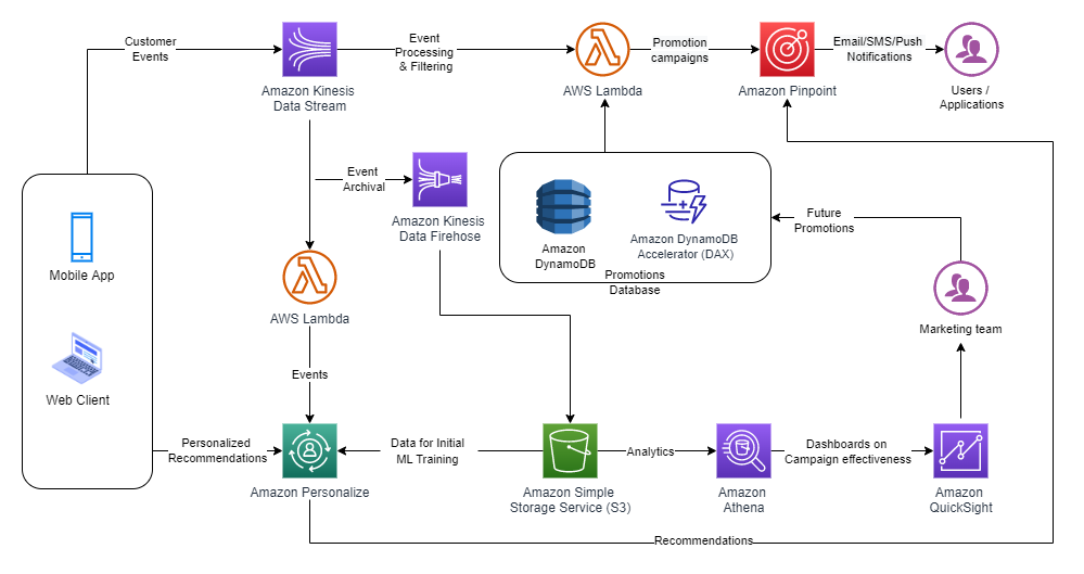
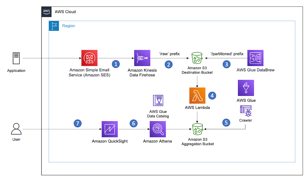
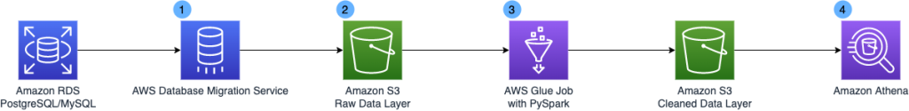
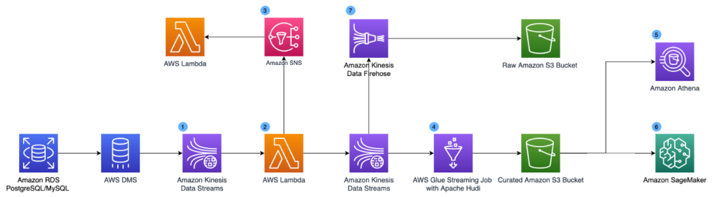
The data can originate from any source, but typically customers want to bring operational data to data lakes to perform data analytics. One of the solutions is to bring the relational data by using AWS Database Migration Service (AWS DMS). AWS DMS tasks can be configured to copy the full load as well as ongoing changes (CDC). The full load and CDC load can be brought into the raw and curated (Delta Lake) storage layers in the data lake. To keep it simple, in this post we opt out of the data sources and ingestion layer; the assumption is that the data is already copied to the raw bucket in the form of CSV files. An AWS Glue ETL job does the necessary transformation and copies the data to the Delta Lake layer. The Delta Lake layer ensures ACID compliance of the source data.
The following diagram illustrates the solution architecture.
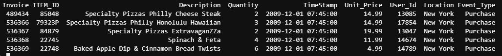
The use case we use in this post is about a commercial insurance company. We use a simple dataset that contains the following columns:
- Policy – Policy number, entered as text
- Expiry – Date that policy expires
- Location – Location type (Urban or Rural)
- State – Name of state where property is located
- Region – Geographic region where property is located
- Insured Value – Property value
- Business Type – Business use type for property, such as Farming or Retail
- Earthquake – Is earthquake coverage included (Y or N)
- Flood – Is flood coverage included (Y or N)
The dataset contains a sample of 25 insurance policies. In the case of a production dataset, it may contain millions of records.
In the following sections, we walk through the steps to perform the Delta Lake UPSERT operations. We use the AWS Management Console to perform all the steps. However, you can also automate these steps using tools like AWS CloudFormation, the AWS Cloud Development Kit (AWS CDK), Terraforms, and so on.
Prerequisites
This post is focused towards architects, engineers, developers, and data scientists who build, design, and build analytical solutions on AWS. We expect a basic understanding of the console, AWS Glue, Amazon Simple Storage Service (Amazon S3), and Athena. Additionally, the persona is able to create AWS Identity and Access Management (IAM) policies and roles, create and run AWS Glue jobs and crawlers, and is able work with the Athena query editor.
Use Athena query engine version 3 to query delta lake tables, later in the section “Query the full load using Athena”.

Set up an S3 bucket for full and CDC load data feeds
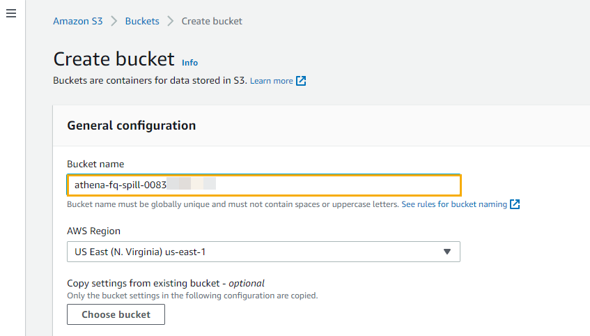
To set up your S3 bucket, complete the following steps:
- Log in to your AWS account and choose a Region nearest to you.
- On the Amazon S3 console, create a new bucket. Make sure the name is unique (for example,
delta-lake-cdc-blog-<some random number>). - Create the following folders:
- $bucket_name/fullload – This folder is used for a one-time full load from the upstream data source
- $bucket_name/cdcload – This folder is used for copying the upstream data changes
- $bucket_name/delta – This folder holds the Delta Lake data files
- Copy the sample dataset and save it in a file called
full-load.csvto your local machine. - Upload the file using the Amazon S3 console into the folder
$bucket_name/fullload.

Set up an IAM policy and role
In this section, we create an IAM policy for the S3 bucket access and a role for AWS Glue jobs to run, and also use the same role for querying the Delta Lake using Athena.
- On the IAM console, choose Polices in the navigation pane.
- Choose Create policy.
- Select JSON tab and paste the following policy code. Replace the
{bucket_name}you created in the earlier step.
- Name the policy
delta-lake-cdc-blog-policyand select Create policy. - On the IAM console, choose Roles in the navigation pane.
- Choose Create role.
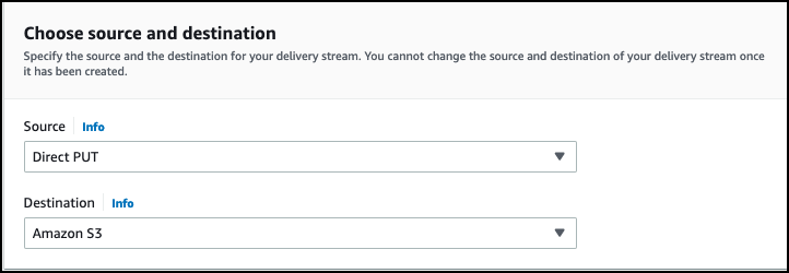
- Select AWS Glue as your trusted entity and choose Next.
- Select the policy you just created, and with two additional AWS managed policies:
delta-lake-cdc-blog-policyAWSGlueServiceRoleCloudWatchFullAccess
- Choose Next.
- Give the role a name (for example,
delta-lake-cdc-blog-role).

Set up AWS Glue jobs
In this section, we set up two AWS Glue jobs: one for full load and one for the CDC load. Let’s start with the full load job.
- On the AWS Glue console, under Data Integration and ETL in the navigation pane, choose Jobs. AWS Glue Studio opens in a new tab.
- Select Spark script editor and choose Create.

- In the script editor, replace the code with the following code snippet
- Navigate to the Job details tab.
- Provide a name for the job (for example,
Full-Load-Job). - For IAM Role¸ choose the role
delta-lake-cdc-blog-rolethat you created earlier. - For Worker type¸ choose G 2X.
- For Job bookmark, choose Disable.
- Set Number of retries to 0.
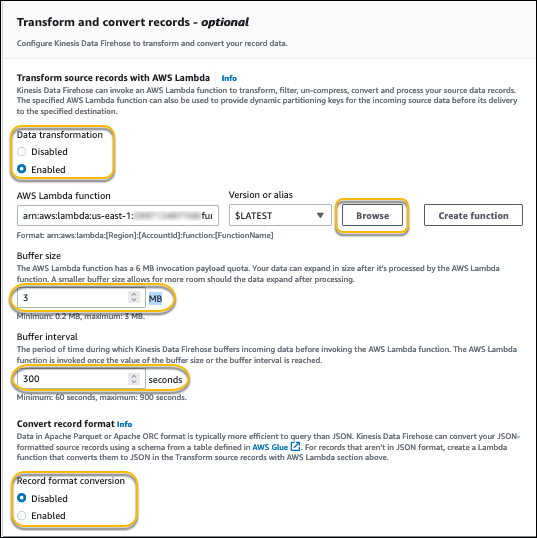
- Under Advanced properties¸ keep the default values, but provide the delta core JAR file path for Python library path and Dependent JARs path.
- Under Job parameters:
- Add the key
--s3_bucketwith the bucket name you created earlier as the value. - Add the key
--datalake-formatsand give the valuedelta
- Add the key
- Keep the remaining default values and choose Save.

Now let’s create the CDC load job.
- Create a second job called
CDC-Load-Job. - Follow the steps on the Job details tab as with the previous job.
- Alternatively, you may choose “Clone job” option from the Full-Load-Job, this will carry all the job details from the full load job.
- In the script editor, enter the following code snippet for the CDC logic:
import sys
from awsglue.utils import getResolvedOptions
from awsglue.context import GlueContext
from pyspark.sql.session import SparkSession
from pyspark.sql.functions import col
from pyspark.sql.functions import expr

## For Delta lake
from delta.tables import DeltaTable


## @params: [JOB_NAME]
args = getResolvedOptions(sys.argv, ['JOB_NAME','s3_bucket'])

# Initialize Spark Session with Delta Lake
spark = SparkSession \
.builder \
.config("spark.sql.extensions", "io.delta.sql.DeltaSparkSessionExtension") \
.config("spark.sql.catalog.spark_catalog", "org.apache.spark.sql.delta.catalog.DeltaCatalog") \
.getOrCreate()

# Read the CDC load
cdc_df = spark.read.csv("s3://"+ args['s3_bucket']+"/cdcload")
cdc_df.show(5,True)

# now read the full load (latest data) as delta table
delta_df = DeltaTable.forPath(spark, "s3://"+ args['s3_bucket']+"/delta/insurance/")
delta_df.toDF().show(5,True)

# UPSERT process if matches on the condition the update else insert
# if there is no keyword then create a data set with Insert, Update and Delete flag and do it separately.
# for delete it has to run in loop with delete condition, this script do not handle deletes.

final_df = delta_df.alias("prev_df").merge( \
source = cdc_df.alias("append_df"), \
#matching on primarykey
condition = expr("prev_df.policy_id = append_df._c1"))\
.whenMatchedUpdate(set= {
    "prev_df.expiry_date"           : col("append_df._c2"),
    "prev_df.location_name"         : col("append_df._c3"),
    "prev_df.state_code"            : col("append_df._c4"),
    "prev_df.region_name"           : col("append_df._c5"),
    "prev_df.insured_value"         : col("append_df._c6"),
    "prev_df.business_type"         : col("append_df._c7"),
    "prev_df.earthquake_coverage"   : col("append_df._c8"),
    "prev_df.flood_coverage"        : col("append_df._c9")} )\
.whenNotMatchedInsert(values =
#inserting a new row to Delta table
{   "prev_df.policy_id"             : col("append_df._c1"),
    "prev_df.expiry_date"           : col("append_df._c2"),
    "prev_df.location_name"         : col("append_df._c3"),
    "prev_df.state_code"            : col("append_df._c4"),
    "prev_df.region_name"           : col("append_df._c5"),
    "prev_df.insured_value"         : col("append_df._c6"),
    "prev_df.business_type"         : col("append_df._c7"),
    "prev_df.earthquake_coverage"   : col("append_df._c8"),
    "prev_df.flood_coverage"        : col("append_df._c9")
})\
.execute()
Run the full load job
On the AWS Glue console, open full-load-job and choose Run. The job takes about 2 minutes to complete, and the job run status changes to Succeeded. Go to $bucket_name and open the delta folder, which contains the insurance folder. You can note the Delta Lake files in it. 
Create and run the AWS Glue crawler
In this step, we create an AWS Glue crawler with Delta Lake as the data source type. After successfully running the crawler, we inspect the data using Athena.
- On the AWS Glue console, choose Crawlers in the navigation pane.
- Choose Create crawler.
- Provide a name (for example,
delta-lake-crawler) and choose Next. - Choose Add a data source and choose Delta Lake as your data source.
- Copy your delta folder URI (for example,
s3://delta-lake-cdc-blog-123456789/delta/insurance) and enter the Delta Lake table path location. - Keep the default selection Create Native tables, and choose Add a Delta Lake data source.
- Choose Next.
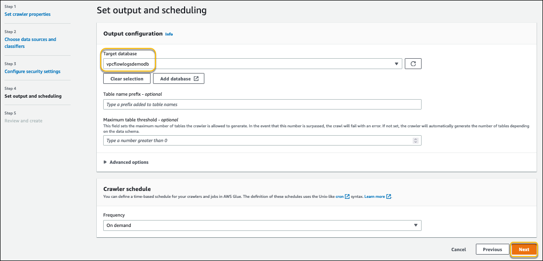
- Choose the IAM role you created earlier, then choose Next.
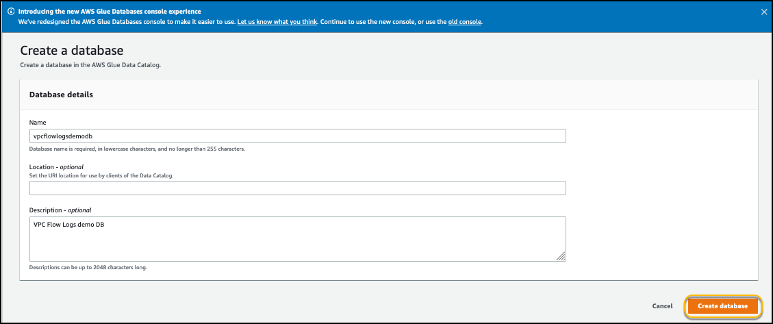
- Select the
defaulttarget database, and providedelta_for the table name prefix. If nodefaultdatabase exist, you may create one. - Choose Next.
- Choose Create crawler.
- Run the newly created crawler. After the crawler is complete, the
delta_insurancetable is available underDatabases/Tables. - Open the table to check the table overview.
You can observe nine columns and their data types. 
Query the full load using Athena
In the earlier step, we created the delta_insurance table by running a crawler against the Delta Lake location. In this section, we query the delta_insurance table using Athena. Note that if you’re using Athena for the first time, set the query output folder to store the Athena query results (for example, s3://<your-s3-bucket>/query-output/).
- On the Athena console, open the query editor.
- Keep the default selections for Data source and Database.
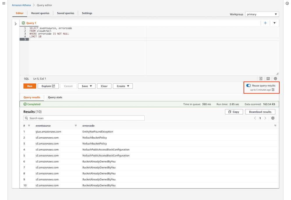
- Run the query
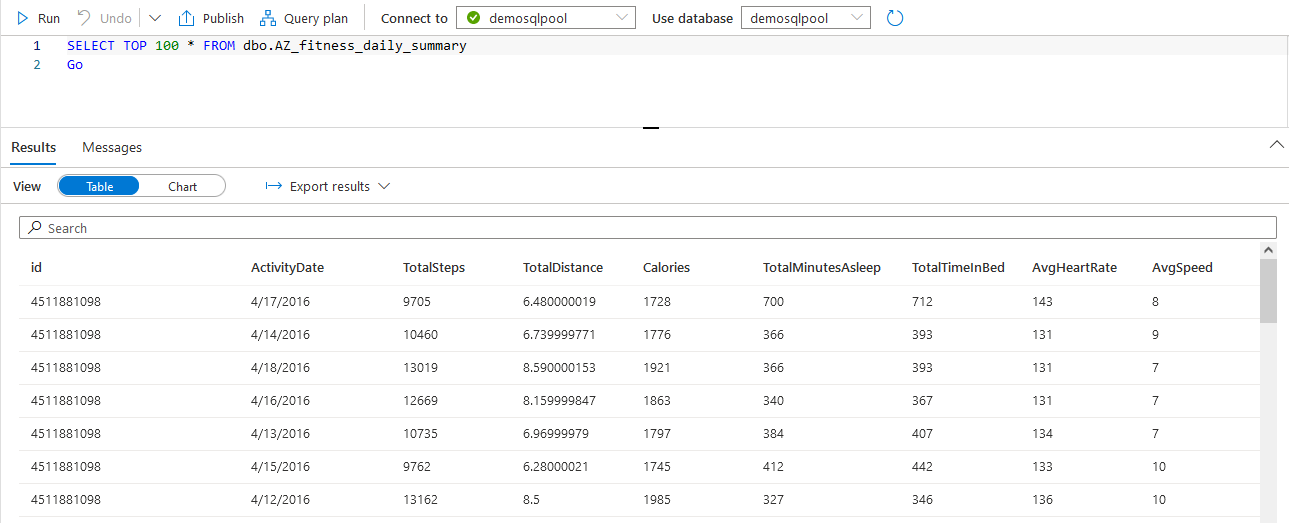
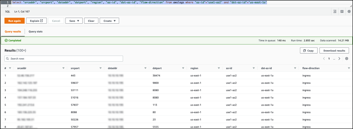
SELECT * FROM delta_insurance;. This query returns a total of 25 rows, the same as what was in the full load data feed. - For the CDC comparison, run the following query and store the results in a location where you can compare these results later:
The following screenshot shows the Athena query result.

Upload the CDC data feed and run the CDC job
In this section, we update three insurance policies and insert two new policies.
- Copy the following insurance policy data and save it locally as
cdc-load.csv:
The first column in the CDC feed describes the UPSERT operations. U is for updating an existing record, and I is for inserting a new record.
- Upload the cdc-load.csv file to the
$bucket_name/cdcload/folder. - On the AWS Glue console, run
CDC-Load-Job. This job takes care of updating the Delta Lake accordingly.
The change details are as follows:
- 100462 – Expiry date changes to 12/31/2024
- 100463 – Insured value changes to 1 million
- 100475 – This policy is now under a new flood zone
- 110001 and 110002 – New policies added to the table
- Run the query again:
As shown in the following screenshot, the changes in the CDC data feed are reflected in the Athena query results.

Clean up
In this solution, we used all managed services, and there is no cost if AWS Glue jobs aren’t running. However, if you want to clean up the tasks, you can delete the two AWS Glue jobs, AWS Glue table, and S3 bucket.
Conclusion
Organizations are continuously looking at high performance, cost-effective, and scalable analytical solutions to extract the value of their operational data sources in near-real time. The analytical platform should be ready to receive changes in the operational data as soon as they occur. Typical data lake solutions face challenges to handle the changes in source data; the Delta Lake framework can close this gap. This post demonstrated how to build data lakes for UPSERT operations using AWS Glue and native Delta Lake tables, and how to query AWS Glue tables from Athena. You can implement your large scale UPSERT data operations using AWS Glue, Delta Lake and perform analytics using Amazon Athena.
References
- Introducing native Delta Lake table support with AWS Glue crawlers
- Build a high-performance, transactional data lake using open-source Delta Lake on Amazon EMR
- Build, Test and Deploy ETL solutions using AWS Glue and AWS CDK based CI/CD pipelines
- What is Delta Lake?
About the Authors
 Praveen Allam is a Solutions Architect at AWS. He helps customers design scalable, better cost-perfromant enterprise-grade applications using the AWS Cloud. He builds solutions to help organizations make data-driven decisions.
 Vivek Singh is Senior Solutions Architect with the AWS Data Lab team. He helps customers unblock their data journey on the AWS ecosystem. His interest areas are data pipeline automation, data quality and data governance, data lakes, and lake house architectures.


 Dylan Qu is a Specialist Solutions Architect focused on big data and analytics with Amazon Web Services. He helps customers architect and build highly scalable, performant, and secure cloud-based solutions on AWS.