Post Syndicated from Sakti Mishra original https://aws.amazon.com/blogs/big-data/unstructured-data-management-and-governance-using-aws-ai-ml-and-analytics-services/
Unstructured data is information that doesn’t conform to a predefined schema or isn’t organized according to a preset data model. Unstructured information may have a little or a lot of structure but in ways that are unexpected or inconsistent. Text, images, audio, and videos are common examples of unstructured data. Most companies produce and consume unstructured data such as documents, emails, web pages, engagement center phone calls, and social media. By some estimates, unstructured data can make up to 80–90% of all new enterprise data and is growing many times faster than structured data. After decades of digitizing everything in your enterprise, you may have an enormous amount of data, but with dormant value. However, with the help of AI and machine learning (ML), new software tools are now available to unearth the value of unstructured data.
In this post, we discuss how AWS can help you successfully address the challenges of extracting insights from unstructured data. We discuss various design patterns and architectures for extracting and cataloging valuable insights from unstructured data using AWS. Additionally, we show how to use AWS AI/ML services for analyzing unstructured data.
Why it’s challenging to process and manage unstructured data
Unstructured data makes up a large proportion of the data in the enterprise that can’t be stored in a traditional relational database management systems (RDBMS). Understanding the data, categorizing it, storing it, and extracting insights from it can be challenging. In addition, identifying incremental changes requires specialized patterns and detecting sensitive data and meeting compliance requirements calls for sophisticated functions. It can be difficult to integrate unstructured data with structured data from existing information systems. Some view structured and unstructured data as apples and oranges, instead of being complementary. But most important of all, the assumed dormant value in the unstructured data is a question mark, which can only be answered after these sophisticated techniques have been applied. Therefore, there is a need to being able to analyze and extract value from the data economically and flexibly.
Solution overview
Data and metadata discovery is one of the primary requirements in data analytics, where data consumers explore what data is available and in what format, and then consume or query it for analysis. If you can apply a schema on top of the dataset, then it’s straightforward to query because you can load the data into a database or impose a virtual table schema for querying. But in the case of unstructured data, metadata discovery is challenging because the raw data isn’t easily readable.
You can integrate different technologies or tools to build a solution. In this post, we explain how to integrate different AWS services to provide an end-to-end solution that includes data extraction, management, and governance.
The solution integrates data in three tiers. The first is the raw input data that gets ingested by source systems, the second is the output data that gets extracted from input data using AI, and the third is the metadata layer that maintains a relationship between them for data discovery.
The following is a high-level architecture of the solution we can build to process the unstructured data, assuming the input data is being ingested to the raw input object store.
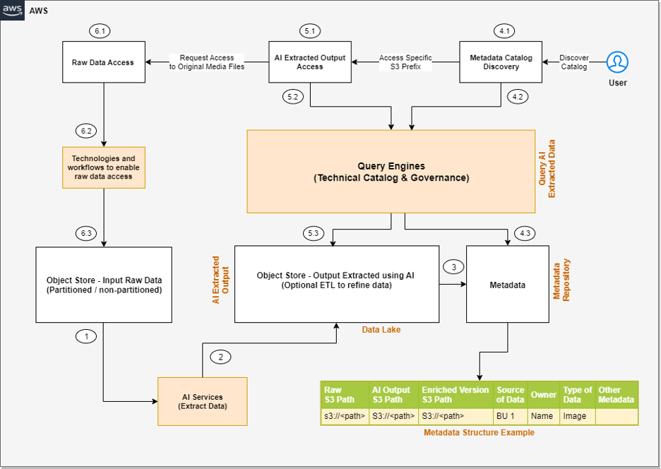
The steps of the workflow are as follows:
- Integrated AI services extract data from the unstructured data.
- These services write the output to a data lake.
- A metadata layer helps build the relationship between the raw data and AI extracted output. When the data and metadata are available for end-users, we can break the user access pattern into additional steps.
- In the metadata catalog discovery step, we can use query engines to access the metadata for discovery and apply filters as per our analytics needs. Then we move to the next stage of accessing the actual data extracted from the raw unstructured data.
- The end-user accesses the output of the AI services and uses the query engines to query the structured data available in the data lake. We can optionally integrate additional tools that help control access and provide governance.
- There might be scenarios where, after accessing the AI extracted output, the end-user wants to access the original raw object (such as media files) for further analysis. Additionally, we need to make sure we have access control policies so the end-user has access only to the respective raw data they want to access.
Now that we understand the high-level architecture, let’s discuss what AWS services we can integrate in each step of the architecture to provide an end-to-end solution.
The following diagram is the enhanced version of our solution architecture, where we have integrated AWS services.

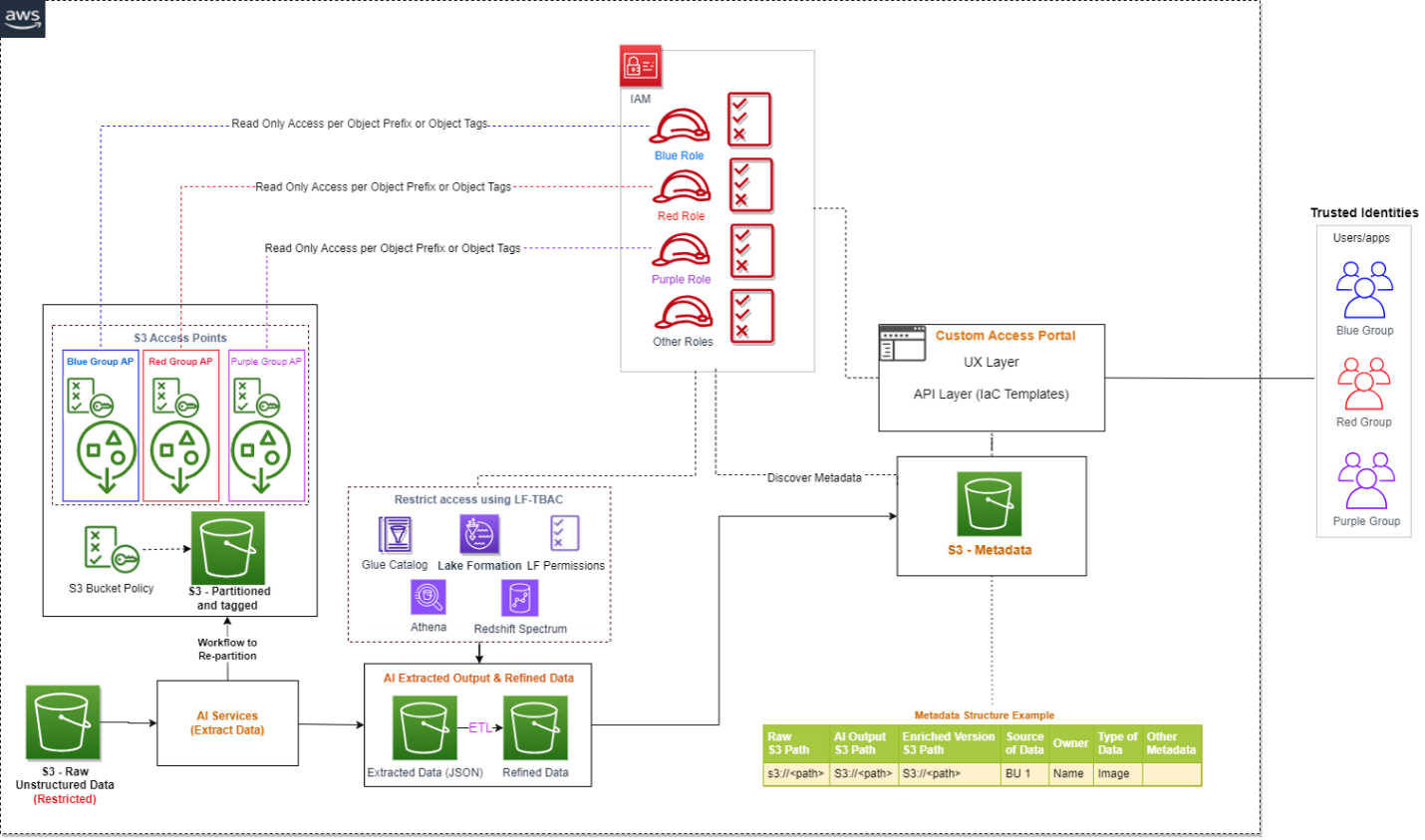
Let’s understand how these AWS services are integrated in detail. We have divided the steps into two broad user flows: data processing and metadata enrichment (Steps 1–3) and end-users accessing the data and metadata with fine-grained access control (Steps 4–6).
- Various AI services (which we discuss in the next section) extract data from the unstructured datasets.
- The output is written to an Amazon Simple Storage Service (Amazon S3) bucket (labeled Extracted JSON in the preceding diagram). Optionally, we can restructure the input raw objects for better partitioning, which can help while implementing fine-grained access control on the raw input data (labeled as the Partitioned bucket in the diagram).
- After the initial data extraction phase, we can apply additional transformations to enrich the datasets using AWS Glue. We also build an additional metadata layer, which maintains a relationship between the raw S3 object path, the AI extracted output path, the optional enriched version S3 path, and any other metadata that will help the end-user discover the data.
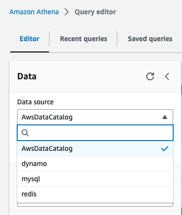
- In the metadata catalog discovery step, we use the AWS Glue Data Catalog as the technical catalog, Amazon Athena and Amazon Redshift Spectrum as query engines, AWS Lake Formation for fine-grained access control, and Amazon DataZone for additional governance.
- The AI extracted output is expected to be available as a delimited file or in JSON format. We can create an AWS Glue Data Catalog table for querying using Athena or Redshift Spectrum. Like the previous step, we can use Lake Formation policies for fine-grained access control.
- Lastly, the end-user accesses the raw unstructured data available in Amazon S3 for further analysis. We have proposed integrating Amazon S3 Access Points for access control at this layer. We explain this in detail later in this post.
Now let’s expand the following parts of the architecture to understand the implementation better:
- Using AWS AI services to process unstructured data
- Using S3 Access Points to integrate access control on raw S3 unstructured data
Process unstructured data with AWS AI services
As we discussed earlier, unstructured data can come in a variety of formats, such as text, audio, video, and images, and each type of data requires a different approach for extracting metadata. AWS AI services are designed to extract metadata from different types of unstructured data. The following are the most commonly used services for unstructured data processing:
- Amazon Comprehend – This natural language processing (NLP) service uses ML to extract metadata from text data. It can analyze text in multiple languages, detect entities, extract key phrases, determine sentiment, and more. With Amazon Comprehend, you can easily gain insights from large volumes of text data such as extracting product entity, customer name, and sentiment from social media posts.
- Amazon Transcribe – This speech-to-text service uses ML to convert speech to text and extract metadata from audio data. It can recognize multiple speakers, transcribe conversations, identify keywords, and more. With Amazon Transcribe, you can convert unstructured data such as customer support recordings into text and further derive insights from it.
- Amazon Rekognition – This image and video analysis service uses ML to extract metadata from visual data. It can recognize objects, people, faces, and text, detect inappropriate content, and more. With Amazon Rekognition, you can easily analyze images and videos to gain insights such as identifying entity type (human or other) and identifying if the person is a known celebrity in an image.
- Amazon Textract – You can use this ML service to extract metadata from scanned documents and images. It can extract text, tables, and forms from images, PDFs, and scanned documents. With Amazon Textract, you can digitize documents and extract data such as customer name, product name, product price, and date from an invoice.
- Amazon SageMaker – This service enables you to build and deploy custom ML models for a wide range of use cases, including extracting metadata from unstructured data. With SageMaker, you can build custom models that are tailored to your specific needs, which can be particularly useful for extracting metadata from unstructured data that requires a high degree of accuracy or domain-specific knowledge.
- Amazon Bedrock – This fully managed service offers a choice of high-performing foundation models (FMs) from leading AI companies like AI21 Labs, Anthropic, Cohere, Meta, Stability AI, and Amazon with a single API. It also offers a broad set of capabilities to build generative AI applications, simplifying development while maintaining privacy and security.
With these specialized AI services, you can efficiently extract metadata from unstructured data and use it for further analysis and insights. It’s important to note that each service has its own strengths and limitations, and choosing the right service for your specific use case is critical for achieving accurate and reliable results.
AWS AI services are available via various APIs, which enables you to integrate AI capabilities into your applications and workflows. AWS Step Functions is a serverless workflow service that allows you to coordinate and orchestrate multiple AWS services, including AI services, into a single workflow. This can be particularly useful when you need to process large amounts of unstructured data and perform multiple AI-related tasks, such as text analysis, image recognition, and NLP.
With Step Functions and AWS Lambda functions, you can create sophisticated workflows that include AI services and other AWS services. For instance, you can use Amazon S3 to store input data, invoke a Lambda function to trigger an Amazon Transcribe job to transcribe an audio file, and use the output to trigger an Amazon Comprehend analysis job to generate sentiment metadata for the transcribed text. This enables you to create complex, multi-step workflows that are straightforward to manage, scalable, and cost-effective.
The following is an example architecture that shows how Step Functions can help invoke AWS AI services using Lambda functions.
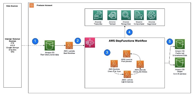
The workflow steps are as follows:
- Unstructured data, such as text files, audio files, and video files, are ingested into the S3 raw bucket.
- A Lambda function is triggered to read the data from the S3 bucket and call Step Functions to orchestrate the workflow required to extract the metadata.
- The Step Functions workflow checks the type of file, calls the corresponding AWS AI service APIs, checks the job status, and performs any postprocessing required on the output.
- AWS AI services can be accessed via APIs and invoked as batch jobs. To extract metadata from different types of unstructured data, you can use multiple AI services in sequence, with each service processing the corresponding file type.
- After the Step Functions workflow completes the metadata extraction process and performs any required postprocessing, the resulting output is stored in an S3 bucket for cataloging.
Next, let’s understand how can we implement security or access control on both the extracted output as well as the raw input objects.
Implement access control on raw and processed data in Amazon S3
We just consider access controls for three types of data when managing unstructured data: the AI-extracted semi-structured output, the metadata, and the raw unstructured original files. When it comes to AI extracted output, it’s in JSON format and can be restricted via Lake Formation and Amazon DataZone. We recommend keeping the metadata (information that captures which unstructured datasets are already processed by the pipeline and available for analysis) open to your organization, which will enable metadata discovery across the organization.
To control access of raw unstructured data, you can integrate S3 Access Points and explore additional support in the future as AWS services evolve. S3 Access Points simplify data access for any AWS service or customer application that stores data in Amazon S3. Access points are named network endpoints that are attached to buckets that you can use to perform S3 object operations. Each access point has distinct permissions and network controls that Amazon S3 applies for any request that is made through that access point. Each access point enforces a customized access point policy that works in conjunction with the bucket policy that is attached to the underlying bucket. With S3 Access Points, you can create unique access control policies for each access point to easily control access to specific datasets within an S3 bucket. This works well in multi-tenant or shared bucket scenarios where users or teams are assigned to unique prefixes within one S3 bucket.
An access point can support a single user or application, or groups of users or applications within and across accounts, allowing separate management of each access point. Every access point is associated with a single bucket and contains a network origin control and a Block Public Access control. For example, you can create an access point with a network origin control that only permits storage access from your virtual private cloud (VPC), a logically isolated section of the AWS Cloud. You can also create an access point with the access point policy configured to only allow access to objects with a defined prefix or to objects with specific tags. You can also configure custom Block Public Access settings for each access point.
The following architecture provides an overview of how an end-user can get access to specific S3 objects by assuming a specific AWS Identity and Access Management (IAM) role. If you have a large number of S3 objects to control access, consider grouping the S3 objects, assigning them tags, and then defining access control by tags.
If you are implementing a solution that integrates S3 data available in multiple AWS accounts, you can take advantage of cross-account support for S3 Access Points.
Conclusion
This post explained how you can use AWS AI services to extract readable data from unstructured datasets, build a metadata layer on top of them to allow data discovery, and build an access control mechanism on top of the raw S3 objects and extracted data using Lake Formation, Amazon DataZone, and S3 Access Points.
In addition to AWS AI services, you can also integrate large language models with vector databases to enable semantic or similarity search on top of unstructured datasets. To learn more about how to enable semantic search on unstructured data by integrating Amazon OpenSearch Service as a vector database, refer to Try semantic search with the Amazon OpenSearch Service vector engine.
As of writing this post, S3 Access Points is one of the best solutions to implement access control on raw S3 objects using tagging, but as AWS service features evolve in the future, you can explore alternative options as well.
About the Authors
 Sakti Mishra is a Principal Solutions Architect at AWS, where he helps customers modernize their data architecture and define their end-to-end data strategy, including data security, accessibility, governance, and more. He is also the author of the book Simplify Big Data Analytics with Amazon EMR. Outside of work, Sakti enjoys learning new technologies, watching movies, and visiting places with family.
 Bhavana Chirumamilla is a Senior Resident Architect at AWS with a strong passion for data and machine learning operations. She brings a wealth of experience and enthusiasm to help enterprises build effective data and ML strategies. In her spare time, Bhavana enjoys spending time with her family and engaging in various activities such as traveling, hiking, gardening, and watching documentaries.
 Sheela Sonone is a Senior Resident Architect at AWS. She helps AWS customers make informed choices and trade-offs about accelerating their data, analytics, and AI/ML workloads and implementations. In her spare time, she enjoys spending time with her family—usually on tennis courts.
 Daniel Bruno is a Principal Resident Architect at AWS. He had been building analytics and machine learning solutions for over 20 years and splits his time helping customers build data science programs and designing impactful ML products.


 This will start a new session with the updated parameters.


 Pathik Shah is a Sr. Analytics Architect on Amazon Athena. He joined AWS in 2015 and has been focusing in the big data analytics space since then, helping customers build scalable and robust solutions using AWS analytics services.
 Raj Devnath is a Product Manager at AWS on Amazon Athena. He is passionate about building products customers love and helping customers extract value from their data. His background is in delivering solutions for multiple end markets, such as finance, retail, smart buildings, home automation, and data communication systems.


 Kartikay Khator is a Solutions Architect on the Global Life Science at Amazon Web Services. He is passionate about helping customers on their cloud journey with focus on AWS analytics services. He is an avid runner and enjoys hiking.
 Kamen Sharlandjiev is a Sr. Big Data and ETL Solutions Architect and Amazon AppFlow expert. He’s on a mission to make life easier for customers who are facing complex data integration challenges. His secret weapon? Fully managed, low-code AWS services that can get the job done with minimal effort and no coding.


 Navnit Shuklaserves as an AWS Specialist Solution Architect with a focus on Analytics. He possesses a strong enthusiasm for assisting clients in discovering valuable insights from their data. Through his expertise, he constructs innovative solutions that empower businesses to arrive at informed, data-driven choices. Notably, Navnit Shukla is the accomplished author of the book titled “Data Wrangling on AWS.
 Patrick Muller works as a Senior Data Lab Architect at AWS. His main responsibility is to assist customers in turning their ideas into a production-ready data product. In his free time, Patrick enjoys playing soccer, watching movies, and traveling.
 Amogh Gaikwad is a Senior Solutions Developer at Amazon Web Services. He helps global customers build and deploy AI/ML solutions on AWS. His work is mainly focused on computer vision, and natural language processing and helping customers optimize their AI/ML workloads for sustainability. Amogh has received his master’s in Computer Science specializing in Machine Learning.


 Ravi Itha is a Principal Consultant at AWS Professional Services with specialization in data and analytics and generalist background in application development. Ravi helps customers with enterprise data strategy initiatives across insurance, airlines, pharmaceutical, and financial services industries. In his 6-year tenure at Amazon, Ravi has helped the AWS builder community by publishing approximately 15 open-source solutions (accessible via
  Srinivas Kandi is a Data Architect at AWS Professional Services. He leads customer engagements related to data lakes, analytics, and data warehouse modernizations. He enjoys reading history and civilizations.


 Shubham Purwar is a Cloud Engineer (ETL) at AWS Bengaluru specialized in AWS Glue and Amazon Athena. He is passionate about helping customers solve issues related to their ETL workload and implement scalable data processing and analytics pipelines on AWS. In his free time, Shubham loves to spend time with his family and travel around the world.
 Nitin Kumar is a Cloud Engineer (ETL) at AWS with a specialization in AWS Glue. He is dedicated to assisting customers in resolving issues related to their ETL workloads and creating scalable data processing and analytics pipelines on AWS.


 Cristiane de Melo is a Solutions Architect Manager at AWS based in Bay Area, CA. She brings 25+ years of experience driving technical pre-sales engagements and is responsible for delivering results to customers. Cris is passionate about working with customers, solving technical and business challenges, thriving on building and establishing long-term, strategic relationships with customers and partners.
 Archana Inapudi is a Senior Solutions Architect at AWS supporting Strategic Customers. She has over a decade of experience helping customers design and build data analytics, and database solutions. She is passionate about using technology to provide value to customers and achieve business outcomes.
 Nikita Sur is a Solutions Architect at AWS supporting a Strategic Customer. She is curious to learn new technologies to solve customer problems. She has a Master’s degree in Information Systems – Big Data Analytics and her passion is databases and analytics.
 Zach Mitchell is a Sr. Big Data Architect. He works within the product team to enhance understanding between product engineers and their customers while guiding customers through their journey to develop their enterprise data architecture on AWS.


 Vijay Velpula is a Data Lake Architect with AWS Professional Services. He helps customers building modern data platforms through implementing Big Data & Analytics solutions. Outside of work, he enjoys spending time with family, traveling, hiking and biking.
 Karthikeyan Ramachandran is a Data Architect with AWS Professional Services. He specializes in MPP systems helping Customers build and maintain Data warehouse environments. Outside of work, he likes to binge-watch tv shows and loves playing cricket and volleyball.
 Sriharsh Adari is a Senior Solutions Architect at Amazon Web Services (AWS), where he helps customers work backwards from business outcomes to develop innovative solutions on AWS. Over the years, he has helped multiple customers on data platform transformations across industry verticals. His core area of expertise include Technology Strategy, Data Analytics, and Data Science. In his spare time, he enjoys playing sports, binge-watching TV shows, and playing Tabla.

 Jonathan Wong is a Solutions Architect at AWS assisting with initiatives within Strategic Accounts. He is passionate about solving customer challenges and has been exploring emerging technologies to accelerate innovation.


 Virendhar (Viru) Sivaraman is a strategic Senior Big Data & Analytics Architect with Amazon Web Services. He is passionate about building scalable big data and analytics solutions in the cloud. Besides work, he enjoys spending time with family, hiking & mountain biking.
 Vivek Shrivastava is a Principal Data Architect, Data Lake in AWS Professional Services. He is a Bigdata enthusiast and holds 14 AWS Certifications. He is passionate about helping customers build scalable and high-performance data analytics solutions in the cloud. In his spare time, he loves reading and finds areas for home automation.


 Raj Ramasubbu is a Sr. Analytics Specialist Solutions Architect focused on big data and analytics and AI/ML with Amazon Web Services. He helps customers architect and build highly scalable, performant, and secure cloud-based solutions on AWS. Raj provided technical expertise and leadership in building data engineering, big data analytics, business intelligence, and data science solutions for over 18 years prior to joining AWS. He helped customers in various industry verticals like healthcare, medical devices, life science, retail, asset management, car insurance, residential REIT, agriculture, title insurance, supply chain, document management, and real estate.
 Rahul Sonawane is a Principal Analytics Solutions Architect at AWS with AI/ML and Analytics as his area of specialty.
 Sundeep Kumar is a Sr. Data Architect, Data Lake at AWS, helping customers build data lake and analytics platform and solutions. When not building and designing data lakes, Sundeep enjoys listening music and playing guitar.

 Thomas Burns,
  Aileen Zheng is a Solutions Architect supporting US Federal Civilian Sciences customers at Amazon Web Services (AWS). She partners with customers to provide technical guidance on enterprise cloud adoption and strategy and helps with building well-architected solutions. She is also very passionate about data analytics and machine learning. In her free time, you’ll find Aileen doing pilates, taking her dog Mumu out for a hike, or hunting down another good spot for food! You’ll also see her contributing to projects to support diversity and women in technology.


 Pathik Shah is a Sr. Big Data Architect on Amazon Athena. He joined AWS in 2015 and has been focusing in the big data analytics space since then, helping customers build scalable and robust solutions using AWS analytics services.
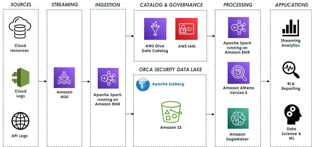
 Eliad Gat is a Big Data & AI/ML Architect at Orca Security. He has over 15 years of experience designing and building large-scale cloud-native distributed systems, specializing in big data, analytics, AI, and machine learning.
 Oded Lifshiz is a Principal Software Engineer at Orca Security. He enjoys combining his passion for delivering innovative, data-driven solutions with his expertise in designing and building large-scale machine learning pipelines.
 Yonatan Dolan is a Principal Analytics Specialist at Amazon Web Services. He is located in Israel and helps customers harness AWS analytical services to leverage data, gain insights, and derive value. Yonatan also leads the Apache Iceberg Israel community.
 Carlos Rodrigues is a Big Data Specialist Solutions Architect at Amazon Web Services. He helps customers worldwide build transactional data lakes on AWS using open table formats like Apache Hudi and Apache Iceberg.
 Sofia Zilberman is a Sr. Analytics Specialist Solutions Architect at Amazon Web Services. She has a track record of 15 years of creating large-scale, distributed processing systems. She remains passionate about big data technologies and architecture trends, and is constantly on the lookout for functional and technological innovations.


 Abdul Qadir is an AWS Solutions Architect based in New Jersey. He works with independent software vendors in the Northeast and provides customer guidance to build well-architected solutions on the AWS cloud platform.
 Sharon Li is a solutions architect at AWS, based in the Boston, MA area. She works with enterprise customers, helping them solve difficult problems and build on AWS. Outside of work, she likes to spend time with her family and explore local restaurants.

 Jacques Steyn runs the Altron Data Analytics Professional Services. He has been leading the building of data warehouses and analytic solutions for the past 20 years. In his free time, he spends time with his family, whether it be on the golf , walking in the mountains, or camping in South Africa, Botswana, and Namibia.
 Jason Yung is a Principal Analytics Specialist with Amazon Web Services. Working with Senior Executives across the Europe and Asia-Pacific Regions, he helps customers become data-driven by understanding their use cases and articulating business value through Amazon mechanisms. In his free time, he spends time looking after a very active 1-year-old daughter, alongside juggling geeky activities with respectable hobbies such as cooking sub-par food.
 Michele Lamarca is a Senior Solutions Architect with Amazon Web Services. He helps architect and run Solutions Accelerators in Europe to enable customers to become hands-on with AWS services and build prototypes quickly to release the value of data in the organization. In his free time, he reads books and tries (hopelessly) to improve his jazz piano skills.
 Hamza is a Specialist Solutions Architect with Amazon Web Services. He runs Solutions Accelerators in EMEA regions to help customers accelerate their journey to move from an idea into a solution in production. In his free time, he spends time with his family, meets with friends, swims in the municipal swimming pool, and learns new skills.


 Rajdip Chaudhuri is a Senior Solutions Architect with Amazon Web Services specializing in data and analytics. He enjoys working with AWS customers and partners on data and analytics requirements. In his spare time, he enjoys soccer and movies.
 Dhiraj Thakur is a Solutions Architect with Amazon Web Services. He works with AWS customers and partners to provide guidance on enterprise cloud adoption, migration, and strategy. He is passionate about technology and enjoys building and experimenting in the analytics and AI/ML space.


 Nishchai JM is an Analytics Specialist Solutions Architect at Amazon Web services. He specializes in building Big-data applications and help customer to modernize their applications on Cloud. He thinks Data is new oil and spends most of his time in deriving insights out of the Data.
 Varad Ram is Senior Solutions Architect in Amazon Web Services. He likes to help customers adopt to cloud technologies and is particularly interested in artificial intelligence. He believes deep learning will power future technology growth. In his spare time, he like to be outdoor with his daughter and son.
 Narendra Gupta is a Specialist Solutions Architect at AWS, helping customers on their cloud journey with a focus on AWS analytics services. Outside of work, Narendra enjoys learning new technologies, watching movies, and visiting new places
 Arun A K is a Big Data Solutions Architect with AWS. He works with customers to provide architectural guidance for running analytics solutions on the cloud. In his free time, Arun loves to enjoy quality time with his family