Tag Archives: Amazon Sagemaker

Building event-driven architectures with IoT sensor data

Post Syndicated from Raghavarao Sodabathina original https://aws.amazon.com/blogs/architecture/building-event-driven-architectures-with-iot-sensor-data/

The Internet of Things (IoT) brings sensors, cloud computing, analytics, and people together to improve productivity and efficiency. It empowers customers with the intelligence they need to build new services and business models, improve products and services over time, understand their customers’ needs to provide better services, and improve customer experiences. Business operations become more efficient by making intelligent decisions more quickly and over time develop a data-driven discipline leading to revenue growth and greater operational efficiency.

In this post, we showcase how to build an event-driven architecture by using AWS IoT services and AWS purpose-built data services. We also discuss key considerations and best practices while building event-driven application architectures with IoT sensor data.

Deriving insights from IoT sensor data

Organizations create value by making decisions from their IoT sensor data in near real time. Some common use cases and solutions that fit under event-driven architecture using IoT sensor data include:

  • Medical device data collection for personalized patient health monitoring, adverse event prediction, and avoidance.
  • Industrial IoT use cases to monitor equipment quality and determine actions like adjusting machine settings, using different sources of raw materials, or performing additional worker training to improve the quality of the factory output.
  • Connected vehicle use cases, such as voice interaction, navigation, location-based services, remote vehicle diagnostics, predictive maintenance, media streaming, and vehicle safety, that are based on in-vehicle computing and near real-time predictive analytics in the cloud.
  • Sustainability and waste reduction solutions, which provide access to dashboards, monitoring systems, data collection, and summarization tools that use machine learning (ML) algorithms to meet sustainability goals. Meeting sustainability goals is paramount for customers in the travel and hospitality industries.

Event-driven reference architecture with IoT sensor data

Figure 1 illustrates how to architect an event-driven architecture with IoT sensor data for near real-time predictive analytics and recommendations.

Building event-driven architecture with IoT sensor data

Figure 1. Building event-driven architecture with IoT sensor data

Architecture flow:

  1. Data originates in IoT devices such as medical devices, car sensors, industrial IoT sensors.This telemetry data is collected using AWS IoT Greengrass, an open-source IoT edge runtime and cloud service that helps your devices collect and analyze data closer to where the data is generated.When an event arrives, AWS IoT Greengrass reacts autonomously to local events, filters and aggregates device data, then communicates securely with the cloud and other local devices in your network to send the data.
  2. Event data is ingested into the cloud using edge-to-cloud interface services such as AWS IoT Core, a managed cloud platform that connects, manages, and scales devices easily and securely.AWS IoT Core interacts with cloud applications and other devices. You can also use AWS IoT SiteWise, a managed service that helps you collect, model, analyze, and visualize data from industrial equipment at scale.
  3. AWS IoT Core can directly stream ingested data into Amazon Kinesis Data Streams. The ingested data gets transformed and analyzed in near real time using Amazon Kinesis Data Analytics with Apache Flink and Apache Beam frameworks.Stream data can further be enriched using lookup data hosted in a data warehouse such as Amazon Redshift. Amazon Kinesis Data Analytics can persist SQL results to Amazon Redshift after the customer’s integration and stream aggregation (for example, one minute or five minutes).The results in Amazon Redshift can be used for further downstream business intelligence (BI) reporting services, such as Amazon QuickSight.
  4. Amazon Kinesis Data Analytics can also write to an AWS Lambda function, which can invoke Amazon SageMaker models. Amazon SageMaker is a the most complete, end-to-end service for machine learning.
  5. Once the ML model is trained and deployed in SageMaker, inferences are invoked in a micro batch using AWS Lambda. Inferenced data is sent to Amazon OpenSearch Service to create personalized monitoring dashboards using Amazon OpenSearch Service dashboards.The transformed IoT sensor data can be stored in Amazon DynamoDB. Customers can use AWS AppSync to provide near real-time data queries to API services for downstream applications. These enterprise applications can be mobile apps or business applications to track and monitor the IoT sensor data in near real-time.Amazon Kinesis Data Analytics can write to an Amazon Kinesis Data Firehose stream, which is a fully managed service for delivering near real-time streaming data to destinations like Amazon Simple Storage Service (Amazon S3), Amazon Redshift, Amazon OpenSearch Service, Splunk, and any custom HTTP endpoints or endpoints owned by supported third-party service providers, including Datadog, Dynatrace, LogicMonitor, MongoDB, New Relic, and Sumo Logic.

    In this example, data from Amazon Kinesis Data Analytics is written to Amazon Kinesis Data Firehose, which micro-batch streams data into an Amazon S3 data lake. The Amazon S3 data lake stores telemetry data for future batch analytics.

Key considerations and best practices

Keep the following best practices in mind:

  • Define the business value from IoT sensor data through interactive discovery sessions with various stakeholders within your organization.
  • Identify the type of IoT sensor data you want to collect and analyze for predictive analytics.
  • Choose the right tools for the job, depending upon your business use case and your data consumers. Please refer to step 5 earlier in this post, where different purpose-built data services were used based on user personas.
  • Consider the event-driven architecture as three key components: event producers, event routers, and event consumers. A producer publishes an event to the router, which filters and pushes the events to consumers. Producer and consumer services are decoupled, which allows them to be scaled, updated, and deployed independently.
  • In this architecture, IoT sensors are event producers. Amazon IoT Greengrass, Amazon IoT Core, Amazon Kinesis Data Streams, and Amazon Kinesis Data Analytics work together as the router from which multiple consumers can consume IoT sensor-generated data. These consumers include Amazon S3 data lakes for telemetry data analysis, Amazon OpenSearch Service for personalized dashboards, and Amazon DynamoDB or AWS AppSync for the downstream enterprise application’s consumption.

Conclusion

In this post, we demonstrated how to build an event-driven architecture with IoT sensor data using AWS IoT services and AWS purpose-built data services. You can now build your own event-driven applications using this post with your IoT sensor data and integrate with your business applications as needed.

Further reading

AWS Week in Review – October 31, 2022

Post Syndicated from Antje Barth original https://aws.amazon.com/blogs/aws/aws-week-in-review-october-31-2022/

No tricks, just treats in this weekly roundup of news and announcements. Let’s switch our AWS Management Console into dark mode and dive right into it.

Last Week’s Launches
Here are some launches that got my attention during the previous week:

AWS Local Zones in Hamburg and Warsaw now generally available – AWS Local Zones help you run latency-sensitive applications closer to end users. The AWS Local Zones in Hamburg, Germany, and Warsaw, Poland, are the first Local Zones in Europe. AWS Local Zones are now generally available in 20 metro areas globally, with announced plans to launch 33 additional Local Zones in metro areas around the world. See the full list of available and announced AWS Local Zones, and learn how to get started.

Amazon SageMaker multi-model endpoint (MME) now supports GPU instances – MME is a managed capability of SageMaker Inference that lets you deploy thousands of models on a single endpoint. MMEs can now run multiple models on a GPU core, share GPU instances behind an endpoint across multiple models, and dynamically load and unload models based on the incoming traffic. This can help you reduce costs and achieve better price performance. Learn how to run multiple deep learning models on GPU with Amazon SageMaker multi-model endpoints.

Amazon EC2 now lets you replace the root Amazon EBS volume for a running instance – You can now use the Replace Root Volume for patching features in Amazon EC2 to replace your instance root volume using an updated AMI without needing to stop the instance. This makes patching of the guest operating system and applications easier, while retraining the instance store data, networking, and IAM configuration. Check out the documentation to learn more.

AWS Fault Injection Simulator now supports network connectivity disruption – AWS Fault Injection Simulator (FIS) is a managed service for running controlled fault injection experiments on AWS. AWS FIS now has a new action type to disrupt network connectivity and validate that your applications are resilient to a total or partial loss of connectivity. To learn more, visit Network Actions in the AWS FIS user guide.

Amazon SageMaker Automatic Model Tuning now supports Grid Search – SageMaker Automatic Model Tuning helps you find the hyperparameter values that result in the best-performing model for a chosen metric. Until now, you could choose between random, Bayesian, and hyperband search strategies. Grid search now lets you cover every combination of the specified hyperparameter values for use cases in which you need reproducible tuning results. Learn how Amazon SageMaker Automatic Model Tuning now supports grid search.

For a full list of AWS announcements, be sure to keep an eye on the What’s New at AWS page.

Other AWS News
Here are some additional news items that you may find interesting:

Celebrating over 20 years of AI/ML innovation – On October 25, we hosted the AWS AI/ML Innovation Day. Bratin Saha and other leaders in the field shared the great strides we have made in the past and discussed what’s next in the world of ML. You can watch the recording here.

AWS open-source news and updates – My colleague Ricardo Sueiras writes this weekly open-source newsletter in which he highlights new open-source projects, tools, and demos from the AWS Community. Read edition #133 here.

Upcoming AWS Events
Check your calendars and sign up for these AWS events:

AWS re:Invent is only 4 weeks away! Join us live in Las Vegas from November 28–December 2 for keynote announcements, training and certification opportunities, access to 1,500+ technical sessions, and much more. Seats are still available to reserve, and walk-ups are available onsite. You can also join us online to watch live keynotes and leadership sessions.

If you are into machine learning like me, check out the ML attendee guide. AWS Machine Learning Hero Vinicius Caridá put together recommended sessions and tips and tricks for building your agenda. We also have attendee guides on additional topics and industries.

On November 2, there is a virtual event for building modern .NET applications on AWS. You can register for free.

On November 11–12, AWS User Groups in India are hosting the AWS Community Day India 2022, with success stories, use cases, and much more from industry leaders. Sign up for free to join this virtual event.

That’s all for this week. Check back next Monday for another Week in Review!

— Antje

This post is part of our Week in Review series. Check back each week for a quick roundup of interesting news and announcements from AWS!

AWS Week in Review – October 10, 2022

Post Syndicated from Marcia Villalba original https://aws.amazon.com/blogs/aws/aws-week-in-review-october-10-2022/

This post is part of our Week in Review series. Check back each week for a quick roundup of interesting news and announcements from AWS!

I had an amazing start to the week last week as I was speaking at the AWS Community Day NL. This event had 500 attendees and over 70 speakers, and Dr. Werner Vogels, Amazon CTO, delivered the keynote. AWS Community Days are community-led conferences organized by local communities, with a variety of workshops and sessions. I recommend checking your region for any of these events.

Community Day NL

Last Week’s Launches
Here are some launches that got my attention during the previous week.

Amazon S3 Object Lambda now supports using your own code to change the results of HEAD and LIST requests, besides GET (which we launched last year). This feature now enables more capabilities for what you can do with S3 Object Lambda. Danilo made a Twitter thread with lots of use cases for this new launch.

Amazon SageMaker Clarify now can provide near real-time explanations for ML predictions. SageMaker Clarify is a service that provides explainability by ML models individual predictions. These explanations are important for developers to get visibility into their training data and models to identify potential bias.

AWS Storage Gateway now supports 15 TiB tapes. It increased the maximum supported virtual tape size on Tape Gateway from 5 TiB to 15 TiB, so you can store more data on a single virtual tape, and you can reduce the number of tapes you need to manage.

Amazon Aurora Serverless v2 now supports AWS CloudFormation. Early this year, we announced the general availability of Aurora Serverless v2, and now you can use AWS CloudFormation Templates to deploy and change the database along with the rest of your infrastructure.

AWS Config now supports 15 new resource types, including AWS DataSync, Amazon GuardDuty, Amazon Simple Email Service (Amazon SES), AWS AppSync, AWS Cloud Map, Amazon EC2, and AWS AppConfig. With this launch, you can use AWS Config to monitor configuration data for the supported resource types in your AWS account, and you can see how the configuration changes.

For a full list of AWS announcements, be sure to keep an eye on the What’s New at AWS page.

Other AWS News
Some other updates and news that you may have missed:

This week an article about how AWS is leading a pilot project to turn the Greek island of Naxos into a smart island caught my attention. The project introduces smart solutions for mobility, primary healthcare, and the transport of goods. The solution has been built based on four pillars that were important for the island: sustainability, telehealth, leisure, and digital skills. Check out the whole article to learn what they are doing.

Podcast Charlas Técnicas de AWS – If you understand Spanish, this podcast is for you. Podcast Charlas Técnicas is one of the official AWS podcasts in Spanish, and every other week there is a new episode. The podcast is meant for builders, and it shares stories about how customers implemented and learned AWS services, how to architect applications, and how to use new services. You can listen to all the episodes directly from your favorite podcast app or at AWS Podcasts en español.

AWS open-source news and updates – This is a newsletter curated by my colleague Ricardo to bring you the latest open-source projects, posts, events, and more.

Upcoming AWS Events
Check your calendars and sign up for these AWS events:

AWS re:Invent reserved seating opens on October 11. If you are planning to attend, book a spot in advance for your favorite sessions. AWS re:Invent is our biggest conference of the year, it happens in Las Vegas from November 28 to December 2, and registrations are open. Many writers of this blog have sessions at re:Invent, and you can search the event agenda using our names.

I started the post talking about AWS Community Days, and there is one in Warsaw, Poland, on October 14. If you are around Warsaw during this week, you can first check out the AWS Pop-up Hub in Warsaw that runs October 10-14 and then join for the Community Day.

On October 20, there is a virtual event for modernizing .NET workloads with Windows containers on AWS, You can register for free.

That’s all for this week. Check back next Monday for another Week in Review!

— Marcia

AWS Week In Review – September 12, 2022

Post Syndicated from Sébastien Stormacq original https://aws.amazon.com/blogs/aws/aws-week-in-review-september-12-2022/

I am working from London, UK, this week to record sessions for the upcoming Innovate EMEA online conference—more about this in a future Week In Review. While I was crossing the channel, I took the time to review what happened on AWS last week.

Last Week’s Launches
Here are some launches that got my attention:

Seekable OCI for lazy loading container images. Seekable OCI (SOCI) is a technology open sourced by AWS that enables containers to launch faster by lazily loading the container image. SOCI works by creating an index of the files within an existing container image. This index is a key enabler to launching containers faster, providing the capability to extract an individual file from a container image before downloading the entire archive. Check out the source code on GitHub.

Amazon Lookout for Metrics now lets you filter data by dimensions and increased the limits on the number of measures and dimensions. Lookout for Metrics uses machine learning (ML) to automatically detect and diagnose anomalies (i.e., outliers from the norm) in business and operational data, such as a sudden dip in sales revenue or customer acquisition rates.

Amazon SageMaker has three new capabilities. First, SageMaker Canvas added additional capabilities to explore and analyze data with advanced visualizations. Second, SageMaker Studio now sends API user identity data to AWS CloudTrail. And third, SageMaker added TensorFlow image classification to its list of builtin algorithms.

The AWS console launches a widget to display the most recent AWS blog posts on the console landing page. Being part of the AWS News Blog team, I couldn’t be more excited about a launch this week. 😀

AW Console Blog widget

Other AWS News
Some other updates and news that you may have missed:

The Amazon Science blog published an article on the design of a pinch grasping robot. It is one of the many areas where we try to improve the efficiency of our fulfillment centers. A must-read if you’re into robotics or logistics.

The Public Sector blog has an article on how Satellogic and AWS are harnessing the power of space and cloud. Satellogic is creating a live catalog of Earth and delivering daily updates to create a complete picture of changes to our planet for decision-makers. Satellogic is generating massive volumes of data, with each of its satellites collecting an average of 50GB of data daily. They are using compute, storage, analytics, and ground station infrastructure in support of their growth.

Event Ruler is now open-source. Talking about open-source, the source code of the core rule engine built first for Amazon CloudWatch Events, and now the core of Amazon Event Bridge, is newly available on GitHub. This is a Java library that allows applications to identify events that match a set of rules. Events and rules are expressed as JSON documents. Rules are compiled for fast evaluation by a finite state engine. Read the announcement blog post to understand how Event Bridge works under the hood.

HP Anyware (formerly Teradici CAS) is now available for Amazon EC2 Mac instances, from the AWS Marketplace. HP Anyware is a remote access solution that provides pixel-perfect rendering for your remote Mac Mini running in the AWS cloud. It uses PCoIP™ to securely and efficiently access the remote macOS machines. You can connect from anywhere, using a PCoIP client application or from thin terminals such as Thin Clients or Zero Clients workstations.

Upcoming AWS Events
Check your calendars and sign up for these AWS events that are happening all over the world:

AWS Summits – Come together to connect, collaborate, and learn about AWS. Registration is open for the following in-person AWS Summits: Mexico City (September 21–22), Bogotá (October 4), and Singapore (October 6).

AWS Community DaysAWS Community Day events are community-led conferences to share and learn with one another. In September, the AWS community in the US will run events in Arlington, Virginia (September 30). In Europe, Community Day events will be held in October. Join us in Amersfoort, Netherlands (October 3), Warsaw, Poland (October 14), and Dresden, Germany (October 19).

That’s all from me for this week. Come back next Monday for another Week in Review!

— seb


This post is part of our Week in Review series. Check back each week for a quick roundup of interesting news and announcements from AWS!

AWS Week in Review – August 29, 2022

Post Syndicated from Antje Barth original https://aws.amazon.com/blogs/aws/aws-week-in-review-august-29-2022/

I’ve just returned from data and machine learning (ML) conferences in Los Angeles and San Francisco, California. It’s been great to chat with customers and developers about the latest technology trends and use cases. This past week has also been packed with launches at AWS.

Last Week’s Launches
Here are some launches that got my attention during the previous week:

Amazon QuickSight announces fine-grained visual embedding. You can now embed individual visuals from QuickSight dashboards in applications and portals to provide key insights to users where they’re needed most. Check out Donnie’s blog post to learn more, and tune into this week’s The Official AWS Podcast episode.

Sample Web App with a Visual

Sample Web App with a Visual

Amazon SageMaker Automatic Model Tuning is now available in the Europe (Milan), Africa (Cape Town), Asia Pacific (Osaka), and Asia Pacific (Jakarta) Regions. In addition, SageMaker Automatic Model Tuning now reuses SageMaker Training instances to reduce start-up overheads by 20x. In scenarios where you have a large number of hyperparameter evaluations, the reuse of training instances can cumulatively save 2 hours for every 50 sequential evaluations.

Amazon RDS now supports setting up connectivity between your RDS database and EC2 compute instance in one click. Amazon RDS automatically sets up your VPC and related network settings during database creation to enable a secure connection between the EC2 instance and the RDS database.

In addition, Amazon RDS for Oracle now supports managed Oracle Data Guard Switchover and Automated Backups for replicas. With the Oracle Data Guard Switchover feature, you can reverse the roles between the primary database and one of its standby databases (replicas) with no data loss and a brief outage. You can also now create Automated Backups and manual DB snapshots of an RDS for Oracle replica, which reduces the time spent taking backups following a role transition.

Amazon Forecast now supports what-if analyses. Amazon Forecast is a fully managed service that uses ML algorithms to deliver highly accurate time series forecasts.  You can now use what-if analyses to quantify the potential impact of business scenarios on your demand forecasts.

AWS Asia Pacific (Jakarta) Region now supports additional AWS services and EC2 instance types – Amazon SageMaker, AWS Application Migration Service, AWS Glue, Red Hat OpenShift Service on AWS (ROSA), and Amazon EC2 X2idn and X2iedn instances are now available in the Asia Pacific (Jakarta) Region.

For a full list of AWS announcements, be sure to keep an eye on the What’s New at AWS page.

Other AWS News
Here are some additional news, blog posts, and fun code competitions you may find interesting:

Scaling AI and Machine Learning Workloads with Ray on AWS – This past week, I attended Ray Summit in San Francisco, California, and had great conversations with the community. Check out this blog post to learn more about AWS contributions to the scalability and operational efficiency of Ray on AWS.

Ray on AWS

New AWS Heroes – It’s great to see both new and familiar faces joining the AWS Heroes program, a worldwide initiative that acknowledges individuals who have truly gone above and beyond to share knowledge in technical communities. Get to know them in the blog post!

DFL Bundesliga Data ShootoutDFL Deutsche Fußball Liga launched a code competition, powered by AWS: the Bundesliga Data Shootout. The task: Develop a computer vision model to classify events on the pitch. Join the competition as an individual or in a team and win prizes.

Become an AWS GameDay World Champion – AWS GameDay is an interactive, team-based learning experience designed to put your AWS skills to the test by solving real-world problems in a gamified, risk-free environment. Developers of all skill levels can get in on the action, to compete for worldwide glory, as well as a chance to claim the top prize: an all-expenses-paid trip to AWS re:Invent Las Vegas 2022!

Learn more about the AWS Impact Accelerator for Black Founders from one of the inaugural members of the program in this blog post. The AWS Impact Accelerator is a series of programs designed to help high-potential, pre-seed start-ups led by underrepresented founders succeed.

Upcoming AWS Events
Check your calendars and sign up for these AWS events:

AWS SummitAWS Global Summits – AWS Global Summits are free events that bring the cloud computing community together to connect, collaborate, and learn about AWS.

Registration is open for the following in-person AWS Summits that might be close to you in August and September: Canberra (August 31), Ottawa (September 8), New Delhi (September 9), and Mexico City (September 21–22), Bogotá (October 4), and Singapore (October 6).

AWS Community DayAWS Community DaysAWS Community Day events are community-led conferences that deliver a peer-to-peer learning experience, providing developers with a venue for them to acquire AWS knowledge in their preferred way: from one another.

In September, the AWS community will host events in the Bay Area, California (September 9) and in Arlington, Virginia (September 30). In October, you can join Community Days in Amersfoort, Netherlands (October 3), in Warsaw, Poland (October 14), and in Dresden, Germany (October 19).

That’s all for this week. Check back next Monday for another Week in Review! And maybe I’ll see you at the AWS Community Day here in the Bay Area!

Antje

This post is part of our Week in Review series. Check back each week for a quick roundup of interesting news and announcements from AWS!

How Grillo Built a Low-Cost Earthquake Early Warning System on AWS

Post Syndicated from Marcia Villalba original https://aws.amazon.com/blogs/aws/how-grillo-built-a-low-cost-earthquake-early-warning-system-on-aws/

It is estimated that 50 percent of the injuries caused when a high magnitude earthquake affects an area are because of falls or falling hazards. This means that most of these injuries could have been prevented if the population had a few seconds of warning to take cover. Grillo, a social impact enterprise focused on seismology, created a low-cost solution using AWS that senses earthquakes and alerts the population in real time about the dangers in the area.

Earthquakes can happen at any time, and there are two actions cities can take to mitigate the damages. First is structural refitting, that is, building structures that can resist earthquakes. This solution doesn’t apply to many areas because they require big investments. The second solution is to send an alert to the affected population before the shaking reaches them. Ten to sixty seconds can be enough time for people to take action by getting out of a building, taking cover, or turning off a dangerous machine.

Earthquake Early Warning (EEW) systems provide rapid detection of earthquakes and alert people at risk. However, because of the hardware, infrastructure, and technology involved, traditional EEW systems can cost hundreds of millions of US dollars to deploy—a cost too high for most countries.

Andrés Meira was living in Haiti during the 2010 earthquake that claimed over 100,000 human lives and left many people homeless and injured. It is estimated that the earthquake affected three million people. He later moved to Mexico, where in 2017, he experienced another high-magnitude earthquake. As a result, Andrés founded Grillo to develop an accessible EEW system, and its solution has been operating successfully in Mexico since 2017.

Grillo developed a low-cost EEW system using sensors and cloud computing. This system uses off-the-shelf sensors that are placed in buildings near seismically active zones. Grillo sensors cost approximately $300 USD, compared to the traditional seismometers that cost around $10,000 USD. Because of these inexpensive sensors, Grillo can offer a higher density of sensors, which reduces the time needed to issue an alert and gives people more time for action. This benefits the population because higher density increases the accuracy of the location detection, reduces false positives, and reduces times to alert.

How sensors are placed

How Grillo sensors are placed

Grillo’s sensors transmit data to the cloud as the shaking is happening. The cloud platform Grillo built on AWS uses machine learning models that can determine and alert in almost real time, with an average latency of 2 to 3 seconds if an earthquake is happening, depending on the data sent by the different sensors. When the cloud platform detects earthquake risk, it sends alerts to nearby populations via a native phone application, IoT loudspeakers placed in populated areas, or by SMS.

Grillo data flow

How data flows from the shaking to the end users

OpenEEW
In addition, Grillo founded the OpenEEW initiative to enable EEW systems for millions of people who live in areas with earthquake risks. This features the sensor hardware schematics, firmware, dashboard, and other elements of the system as open source, with a permissive license for anyone to use freely.

In this initiative, they also share on the Registry of Open Data on AWS all the data produced from the sensors deployed in Mexico, Chile, Puerto Rico, and Costa Rica for different organizations to learn from it and also to train machine learning models.

Low cost sensor

Low-cost sensor

Grillo in Haiti
Haiti ranks among the countries with the highest seismic risk in the world. Large magnitude earthquakes hit Haiti in 2020 and 2021. Currently, Grillo is working to establish their low-cost EEW system in southern Haiti, where most of the large seismic events in the past decade have occurred. This area is home to over three million people.

Over the course of 2021, Grillo installed over 100 sensors in Puerto Rico. And during 2022, they have focused on deploying sensors in the nationwide cell tower network of Haiti. Also during this year, they will calibrate the machine learning models with data from the new sensors in order to correctly predict when there is earthquake risk. Finally, they will develop an SMS alert system with Digicel, a local telecommunication company. Grillo plans to complete the deployment of the south Haiti EEW system by the end of 2022.

School in southern Haiti where alarm systems are placed

School in southern Haiti where alarm systems are placed

Learn more
Grillo partnered with the AWS Disaster Response team to achieve their goals. AWS helped Grillo to migrate their initial system to AWS and provided expert technical assistance on how to use Amazon SageMaker and AWS IoT services. AWS also provided credits to run the system and financial help to build the sensors.

Check the AWS Disaster Response page to learn more about the projects they are currently working on. And visit the Grillo home page to learn more about their EEW system.

Marcia

AWS Week in Review – August 15, 2022

Post Syndicated from Channy Yun original https://aws.amazon.com/blogs/aws/aws-week-in-review-august-15-2022/

I love the AWS Twitch channel for watching interesting online live shows such as AWS On Air, Containers from the Couch, and Serverless Office Hours.

Last week, AWS Storage Day 2022 was hosted virtually on the AWS Twitch channel and covered recent announcements and insights that address customers’ needs to reduce and optimize storage costs and build data resiliency into their organization. For example, we pre-announced Amazon File Cache, an upcoming new service on AWS that accelerates and simplifies hybrid cloud workloads. To learn more, watch the on-demand recording.

Two weeks ago, AWS Silicon Innovation Day 2022 was also hosted on the AWS Twitch channel. This event covered an overview of our history of silicon development and provided useful sessions on specific AWS chip innovations such as AWS NitroAWS GravitonAWS Inferencia, and AWS Trainium. To learn more, watch the on-demand recording. If you don’t miss such useful live events or online shows, check out the upcoming live schedule!

Last Week’s Launches
Here are some launches that caught my eye last week:

AWS Private 5G – With the general availability of AWS Private 5G, you can easily make your own private mobile networks with a powerful box of hardware and software for 4G/LTE mobile networks. This cool new service lets you easily install, operate, and scale high reliability and low latency of a private cellular network in a matter of days and does not require any specialized expertise. You pay only for the network coverage and capacity that you need.

AWS DeepRacer Student Community Races – Educators and event organizers can now create their own private virtual autonomous racing league for students by powering a 1/18th scale race car driven by reinforcement learning. They can select their own track, race date, and time and invite students to participate through a unique link for their event. To learn more, see the AWS DeepRacer Developer Guide.

Amazon SageMaker Updates – Amazon SageMaker Automatic Model Tuning now supports specifying multiple alternate SageMaker training instance types to make tuning jobs more robust when the preferred instance type is not available due to insufficient capacity. SageMaker Model Pipelines supports securely sharing pipeline entities across AWS accounts and access to shared pipelines through direct API calls. SageMaker Canvas expands capabilities to better prepare and analyze data, including replacing missing values and outliers and the flexibility to choose different sample sizes for your datasets.

Amazon Personalize Updates – Amazon Personalize supports incremental bulk dataset imports, a new option for updating your data and improving the quality of your recommendations. Also, Amazon Personalize allows you to promote specific items in all users’ recommendations based on rules that align with your business goals.

AWS Partner Program Updates – We announce the new AWS Transfer Family Delivery Program for AWS Partners that helps customers build sophisticated Managed File Transfer (MFT) and business-to-business (B2B) file exchange solutions with AWS Transfer Family. Also, we introduce the new AWS Supply Chain Competency, featuring top AWS Partners who provide professional services and cloud-native supply chain solutions on AWS.

For a full list of AWS announcements, be sure to keep an eye on the What’s New at AWS page.

Other AWS News
Here are some other news items that you may find interesting:

AWS CDK for Terraform – Two years ago, AWS began collaborating with HashiCorp to develop Cloud Development Kit for Terraform (CDKTF), an open-source tool that provides a developer-friendly workflow for deploying cloud infrastructure with Terraform in their preferred programming language. The CDKTF is now generally available, so try CDK for Terraform and AWS CDK.

Smithy Interface Definition Language (IDL) 2.0 – Smithy is Amazon’s next-generation API modeling language, based on our experience building tens of thousands of services and generating SDKs. This release focuses on improving the developer experience of authoring Smithy models and using code generated from Smithy models.

Serverless Snippets Collection – The AWS Serverless Developer Advocate team introduces the snippets collection to enable reusable, tested, and recommended snippets driven and maintained by the community. Builders can use serverless snippets to find and integrate tools and code examples to help with their development workflow. I recommend searching other useful resources such as Serverless patterns and workflows collection to get started on your serverless application.

Upcoming AWS Events
Check your calendars and sign up for these AWS events:

AWS Summit

AWS Summit – Registration is open for upcoming in-person AWS Summits that might be close to you in August and September: Anaheim (August 18), Chicago (August 28), Canberra (August 31), Ottawa (September 8), New Delhi (September 9), and Mexico City (September 21–22).

AWS Innovate – Data Edition – On August 23, learn how a modern data strategy can support your present and future use cases, including steps to build an end-to-end data solution to store and access, analyze and visualize, and even predict.

AWS Innovate – For Every Application Edition – On August 25, learn about a wide selection of AWS solutions across compute, storage, networking, hybrid, and edge infrastructure to help you scale application resources seamlessly and optimally.

Although these two Innovate events will be held in the Asia Pacific and Japan time zones, you can view on-demand videos for two months following your registration.

Also, we are preparing 16 upcoming online tech talks on August 15–26  to cover a range of topics and expertise levels and feature technical deep dives, demonstrations, customer examples, and live Q&A with AWS experts.

That’s all for this week. Check back next Monday for another Week in Review!

— Channy

This post is part of our Week in Review series. Check back each week for a quick roundup of interesting news and announcements from AWS!

AWS Week in Review – July 4, 2022

Post Syndicated from Marcia Villalba original https://aws.amazon.com/blogs/aws/aws-week-in-review-july-04-2022/

This post is part of our Week in Review series. Check back each week for a quick roundup of interesting news and announcements from AWS!

Summer has arrived in Finland, and these last few days have been hotter than in the Canary Islands! Today in the US it is Independence Day. I hope that if you are celebrating, you’re having a great time. This week I’m very excited about some developer experience and artificial intelligence launches.

Last Week’s Launches
Here are some launches that got my attention during the previous week:

AWS SAM Accelerate is now generally available – SAM Accelerate is a new capability of the AWS Serverless Application Model CLI, which makes it easier for serverless developers to test code changes against the cloud. You can do a hot swap of code directly in the cloud when making a change in your local development environment. This allows you to develop applications faster. Learn more about this launch in the What’s New post.

Amplify UI for React is generally available – Amplify UI is an open-source UI library that helps developers build cloud-native applications. Amplify UI for React comes with over 35 components that you can use, an authentication component that allows you to connect to your backend with no extra configuration, theming for your components. You can also build your UI using Figma. Check the Amplify UI for React site to learn more about all the capabilities offered.

Amazon Connect has new announcements – First, Amazon Connect added support to personalize the flows of the customer experience using Amazon Lex sentiment analysis. It also added support to branch out the flows depending on Amazon Lex confidence scores. Lastly, it added confidence scores to Amazon Connect Customer Profiles to help companies merge duplicate customer records.

Amazon QuickSight – QuickSight authors can now learn and experience Q before signing up. Authors can choose from six different sample topics and explore different visualizations. In addition, QuickSight now supports Level Aware Calculations (LAC) and rolling date functionality. These two new features bring flexibility and simplification to customers to build advanced calculation and dashboards.

Amazon SageMaker – RStudio on SageMaker now allows you to bring your own development environment in a custom image. RStudio on SageMaker is a fully managed RStudio Workbench in the cloud. In addition, SageMaker added four new tabular data modeling algorithms: LightGBM, CatBoost, AutoGluon-Tabular, and TabTransformer to the existing set of built-in algorithms, pre-trained models and pre-built solution templates it provides.

For a full list of AWS announcements, be sure to keep an eye on the What’s New at AWS page.

Other AWS News
Some other updates and news that you may have missed:

AWS Support announced an improved experience when creating a case – There is a new interface for creating support cases in the AWS Support Center console. Now you can create a case with a simplified three-step process that guides you through the flow. Learn more about this new process in the What’s new post.

New AWS Step Functions workflows collection on Serverless Land – The Step Functions workflows collection is a new experience that makes it easier to discover, deploy, and share AWS Step Functions workflows. In this collection, you can find opinionated templates that implement the best practices to build using Step Functions. Learn more about this new collection in Ben’s blog post.

Podcast Charlas Técnicas de AWS – If you understand Spanish, this podcast is for you. Podcast Charlas Técnicas is one of the official AWS Podcasts in Spanish, which shares a new episode ever other week. The podcast is meant for builders, and it shares stories about how customers implement and learn AWS, how to architect applications, and how to use new services. You can listen to all the episodes directly from your favorite podcast app or from the AWS Podcasts en español website.

AWS open-source news and updates – A newsletter curated by my colleague Ricardo brings you the latest open-source projects, posts, events, and more.

Upcoming AWS Events
Check your calendars and sign up for these AWS events:

AWS Summit New York – Join us on July 12 for the in-person AWS Summit. You can register on the AWS Summit page for free.

AWS re:Inforce – This is an in-person learning conference with a focus on security, compliance, identity, and privacy. You can register now to access hundreds of technical sessions, and other content. It will take place July 26 and 27 in Boston, MA.

That’s all for this week. Check back next Monday for another Week in Review!

— Marcia

Image background removal using Amazon SageMaker semantic segmentation

Post Syndicated from Patrick Gryczka original https://aws.amazon.com/blogs/architecture/image-background-removal-using-amazon-sagemaker-semantic-segmentation/

Many individuals are creating their own ecommerce and online stores in order to sell their products and services. This simplifies and speeds the process of getting products out to your selected markets. This is a critical key indicator for the success of your business.

Artificial Intelligence/Machine Learning (AI/ML) and automation can offer you an improved and seamless process for image manipulation. You can take a picture identifying your products. You can then remove the background in order to publish high quality and clean product images. These images can be added to your online stores for consumers to view and purchase. This automated process will drastically decrease the manual effort required, though some manual quality review will be necessary. It will increase your time-to-market (TTM) and quickly get your products out to customers.

This blog post explains how you can automate the removal of image backgrounds by combining semantic segmentation inferences using Amazon SageMaker JumpStart. You can automate image processing using AWS Lambda. We will walk you through how you can set up an Amazon SageMaker JumpStart semantic segmentation inference endpoint using curated training data.

Amazon SageMaker JumpStart solution overview

Solution architecture for automatically processing new images and outputting isolated labels identified through semantic segmentation.

Figure 1. Architecture for automatically processing new images and outputting isolated labels identified through semantic segmentation.

The example architecture in Figure 1 shows a serverless architecture that uses SageMaker to perform semantic segmentation on images. Image processing takes place within a Lambda function, which extracts the identified (product) content from the background content in the image.

In this event driven architecture, Amazon Simple Storage Service (Amazon S3) invokes a Lambda function each time a new product image lands in the Uploaded Image Bucket. That Lambda function calls out to a semantic segmentation endpoint in Amazon SageMaker. The function then receives a segmentation mask that identifies the pixels that are part of the segment we are identifying. Then, the Lambda function processes the image to isolate the identified segment from the rest of the image, outputting the result to our Processed Image Bucket.

Semantic segmentation model

The semantic segmentation algorithm provides a fine-grained, pixel-level approach to developing computer vision applications. It tags every pixel in an image with a class label from a predefined set of classes. Because the semantic segmentation algorithm classifies every pixel in an image, it also provides information about the shapes of the objects contained in the image. The segmentation output is represented as a grayscale image, called a segmentation mask. A segmentation mask is a grayscale image with the same shape as the input image.

You can use the segmentation mask and replace the pixels that correspond to the class that is identified with the pixels from the original image. You can use the Python library PIL to do pixel manipulation on the image. The following images show how the image in Figure 1 will result in the image shown in Figure 2, when passed through semantic segmentation. When you use the Figure 2 mask and replace it with pixels from Figure 1, the end result is the image from Figure 3. Due to minor quality issues of the final image, you will need to do manual cleanup after automation.

Car image with background

Figure 2. Car image with background

Car mask image

Figure 3. Car mask image

Final image, background removed

Figure 4. Final image, background removed

SageMaker JumpStart streamlines the deployment of the prebuilt model on SageMaker, which supports the semantic segmentation algorithm. You can test this using the sample Jupyter notebook available at Extract Image using Semantic Segmentation, which demonstrates how to extract an individual form from the surrounding background.

Learn more about SageMaker JumpStart

SageMaker JumpStart is a quick way to learn about SageMaker features and capabilities through curated one-step solutions, example notebooks, and deployable pre-trained models. You can also fine-tune the models and then deploy them. You can access JumpStart using Amazon SageMaker Studio or programmatically through the SageMaker APIs.

SageMaker JumpStart provides lot of different semantic segmentation models that are pre-trained with class of objects it can identify. These models are fine-tuned for a sample dataset. You can tune the model with your dataset to get an effective mask for the class of object you want to retrieve from the image. When you fine-tune a model, you can use the default dataset or choose your own data, which is located in an Amazon S3 bucket. You can customize the hyperparameters of the training job that are used to fine-tune the model.

When the fine-tuning process is complete, JumpStart provides information about the model: parent model, training job name, training job Amazon Resource Name (ARN), training time, and output path. We retrieve the deploy_image_uri, deploy_source_uri, and base_model_uri for the pre-trained model. You can host the pre-trained base-model by creating an instance of sagemaker.model.Model and deploying it.

Conclusion

In this blog, we review the steps to use Amazon SageMaker JumpStart and AWS Lambda for automation and processing of images. It uses pre-trained machine learning models and inference. The solution ingests the product images, identifies your products, and then removes the image background. After some review and QA, you can then publish your products to your ecommerce store or other medium.

Further resources:

New – Amazon SageMaker Ground Truth Now Supports Synthetic Data Generation

Post Syndicated from Antje Barth original https://aws.amazon.com/blogs/aws/new-amazon-sagemaker-ground-truth-now-supports-synthetic-data-generation/

Today, I am happy to announce that you can now use Amazon SageMaker Ground Truth to generate labeled synthetic image data.

Building machine learning (ML) models is an iterative process that, at a high level, starts with data collection and preparation, followed by model training and model deployment. And especially the first step, collecting large, diverse, and accurately labeled datasets for your model training, is often challenging and time-consuming.

Let’s take computer vision (CV) applications as an example. CV applications have come to play a key role in the industrial landscape. They help improve manufacturing quality or automate warehouses. Yet, collecting the data to train these CV models often takes a long time or can be impossible.

As a data scientist, you might spend months collecting hundreds of thousands of images from the production environments to make sure you capture all variations in data the model will come across. In some cases, finding all data variations might even be impossible, for example, sourcing images of rare product defects, or expensive, if you have to intentionally damage your products to get those images.

And once all data is collected, you need to accurately label the images, which is often a struggle in itself. Manually labeling images is slow and open to human error, and building custom labeling tools and setting up scaled labeling operations can be time-consuming and expensive. One way to mitigate this data challenge is by adding synthetic data to the mix.

Advantages of Combining Real-World Data with Synthetic Data
Combining your real-world data with synthetic data helps to create more complete training datasets for training your ML models.

Synthetic data itself is created by simple rules, statistical models, computer simulations, or other techniques. This allows synthetic data to be created in enormous quantities and with highly accurate labels for annotations across thousands of images. The label accuracy can be done at a very fine granularity, such as on a sub-object or pixel level, and across modalities. Modalities include bounding boxes, polygons, depth, and segments. Synthetic data can also be generated for a fraction of the cost, especially when compared to remote sensing imagery that otherwise relies on satellite, aerial, or drone image collection.

If you combine your real-world data with synthetic data, you can create more complete and balanced data sets, adding data variety that real-world data might lack. With synthetic data, you have the freedom to create any imagery environment, including edge cases that might be difficult to find and replicate in real-world data. You can customize objects and environments with variations, for example, to reflect different lighting, colors, texture, pose, or background. In other words, you can “order” the exact use case you are training your ML model for.

Now, let me show you how you can start sourcing labeled synthetic images using SageMaker Ground Truth.

Get Started on Your Synthetic Data Project with Amazon SageMaker Ground Truth
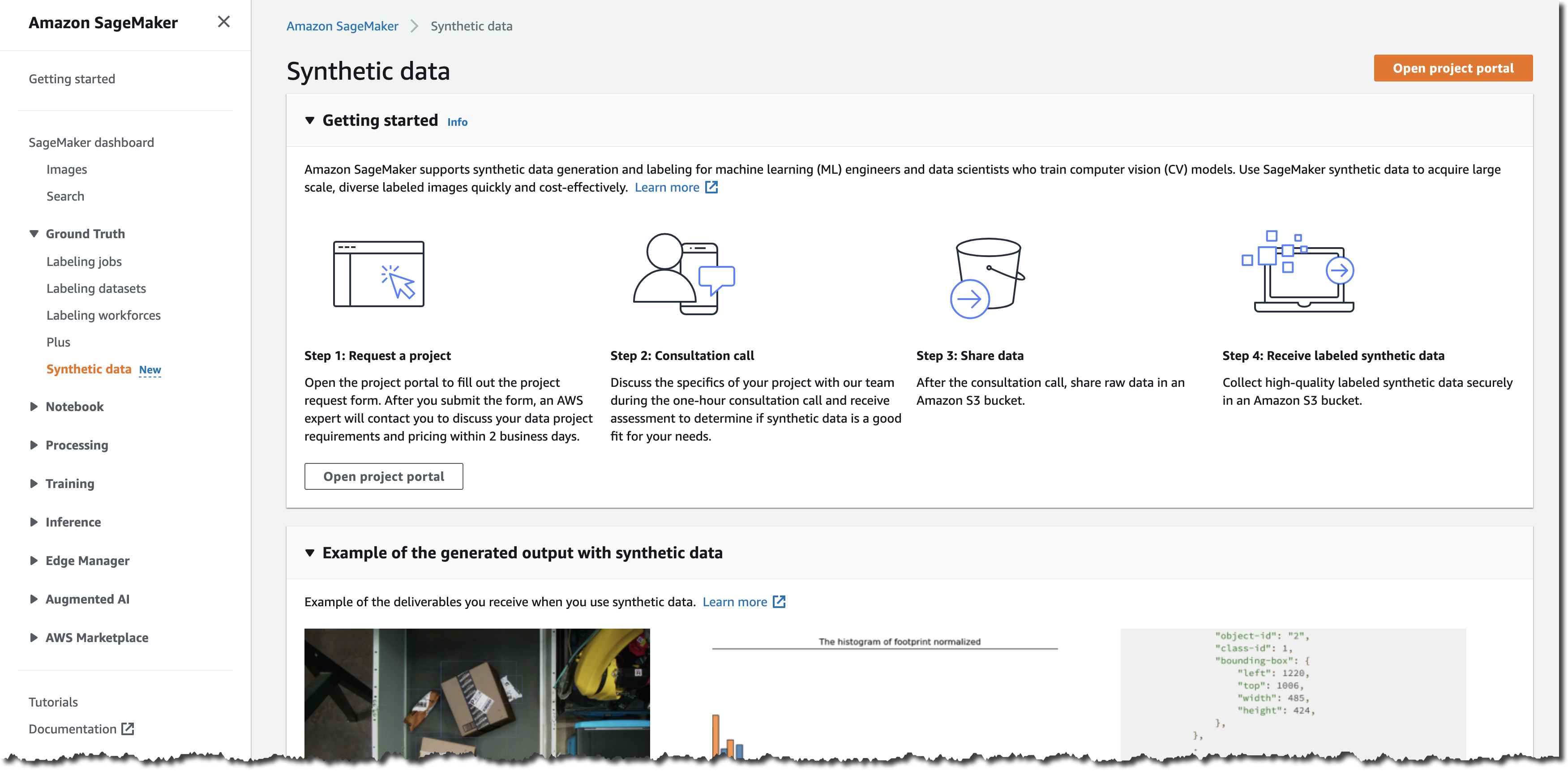
To request a new synthetic data project, navigate to the Amazon SageMaker Ground Truth console and select Synthetic data.

Amazon SageMaker Ground Truth Synthetic Data

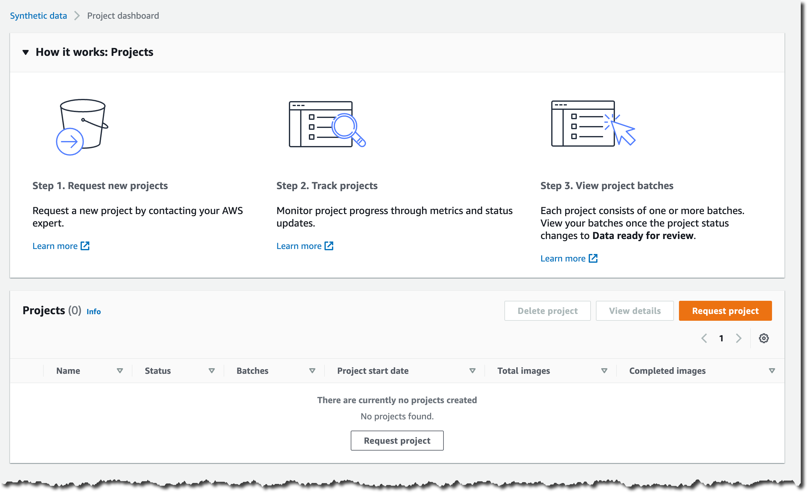
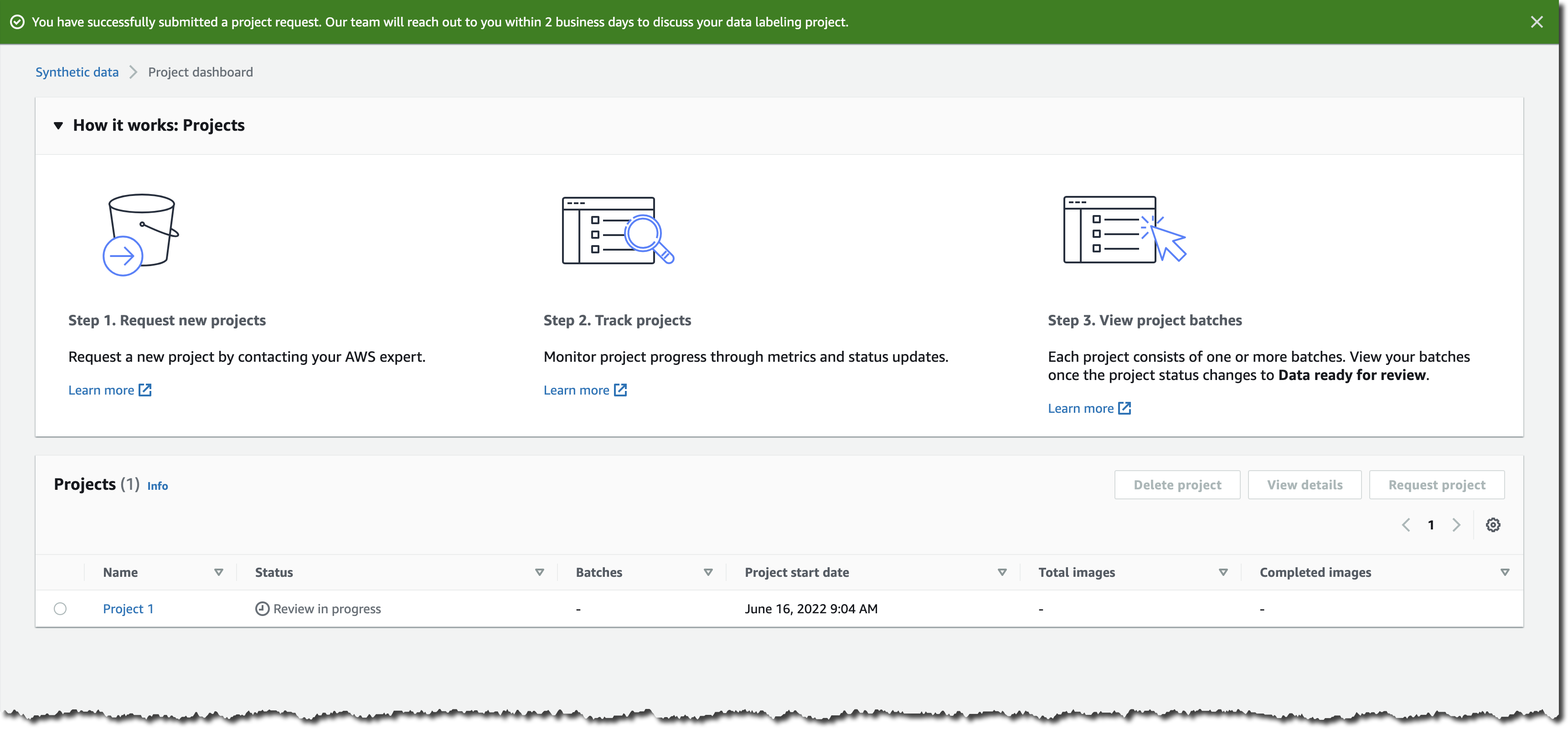
Then, select Open project portal. In the project portal, you can request new projects, monitor projects that are in progress, and view batches of generated images once they become available for review. To initiate a new project, select Request project.

Amazon SageMaker Ground Truth Synthetic Data Project Portal

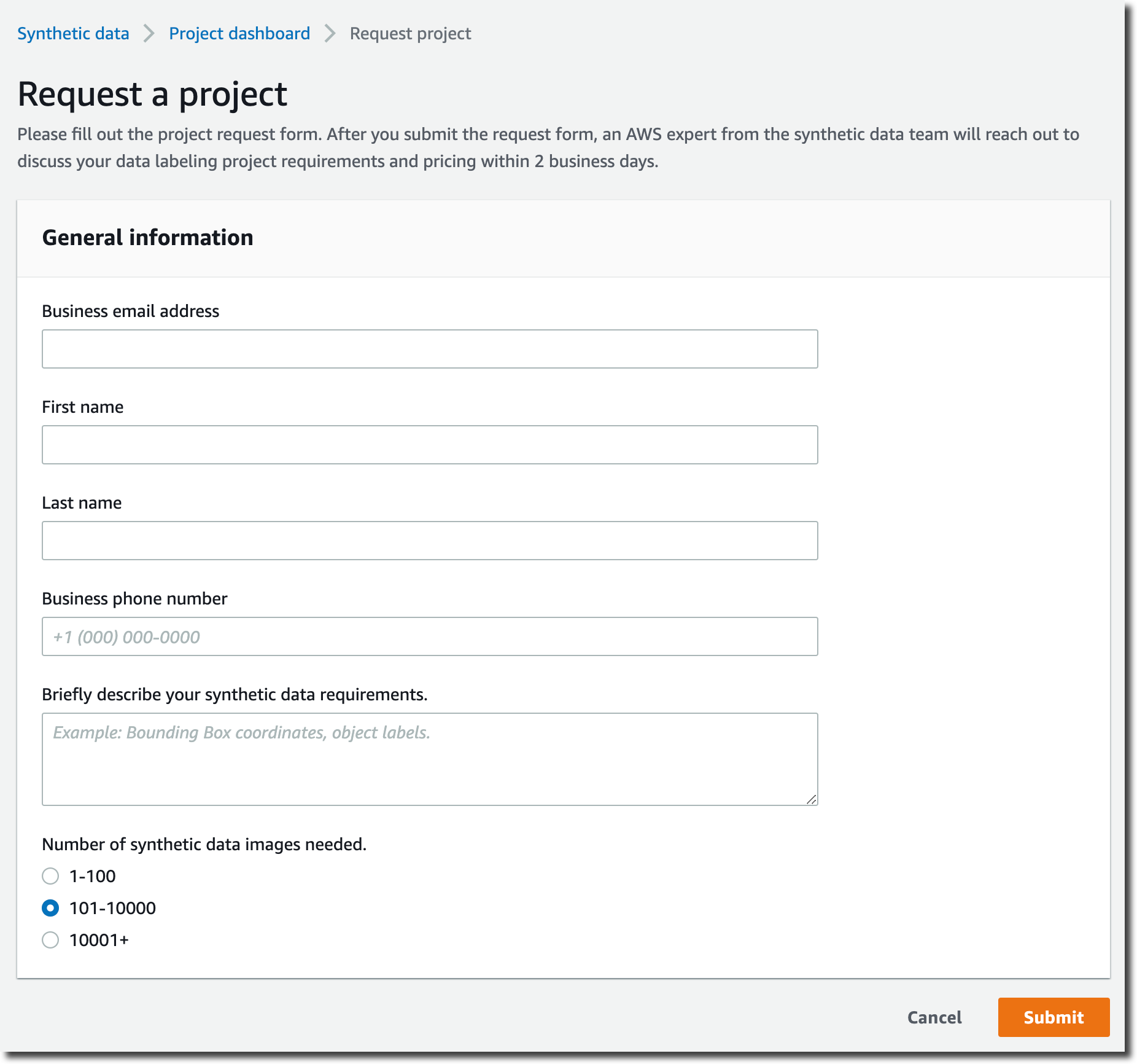
Describe your synthetic data needs and provide contact information.

Request a synthetic data project

After you submit the request form, you can check your project status in the project dashboard.

Amazon SageMaker Ground Truth Synthetic Data Project Created

In the next step, an AWS expert will reach out to discuss your project requirements in more detail. Upon review, the team will share a custom quote and project timeline.

If you want to continue, AWS digital artists will start by creating a small test batch of labeled synthetic images as a pilot production for you to review.

They collect your project inputs, such as reference photos and available 2D and 3D assets. The team then customizes those assets, adds the specified inclusions, such as scratches, dents, and textures, and creates the configuration that describes all the variations that need to be generated.

They can also create and add new objects based on your requirements, configure distributions and locations of objects in a scene, as well as modify object size, shape, color, and surface texture.

Once the objects are prepared, they are rendered using a photorealistic physics engine, capturing an image of the scene from a sensor that is placed in the virtual world. Images are also automatically labeled. Labels include 2D bounding boxes, instance segmentation, and contours.

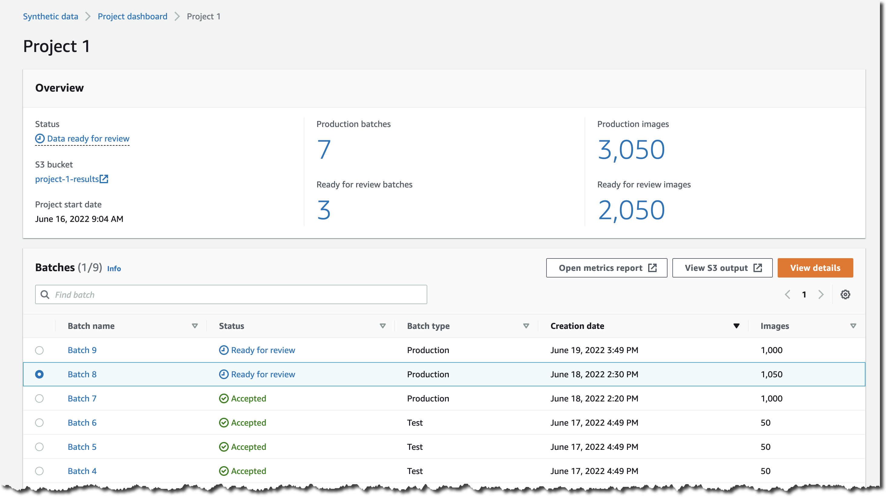
You can monitor the progress of the data generation jobs on the project detail page. Once the pilot production test batch becomes available for review, you can spot-check the images and provide feedback for any rework that might be required.

Review available batches of synthetic data

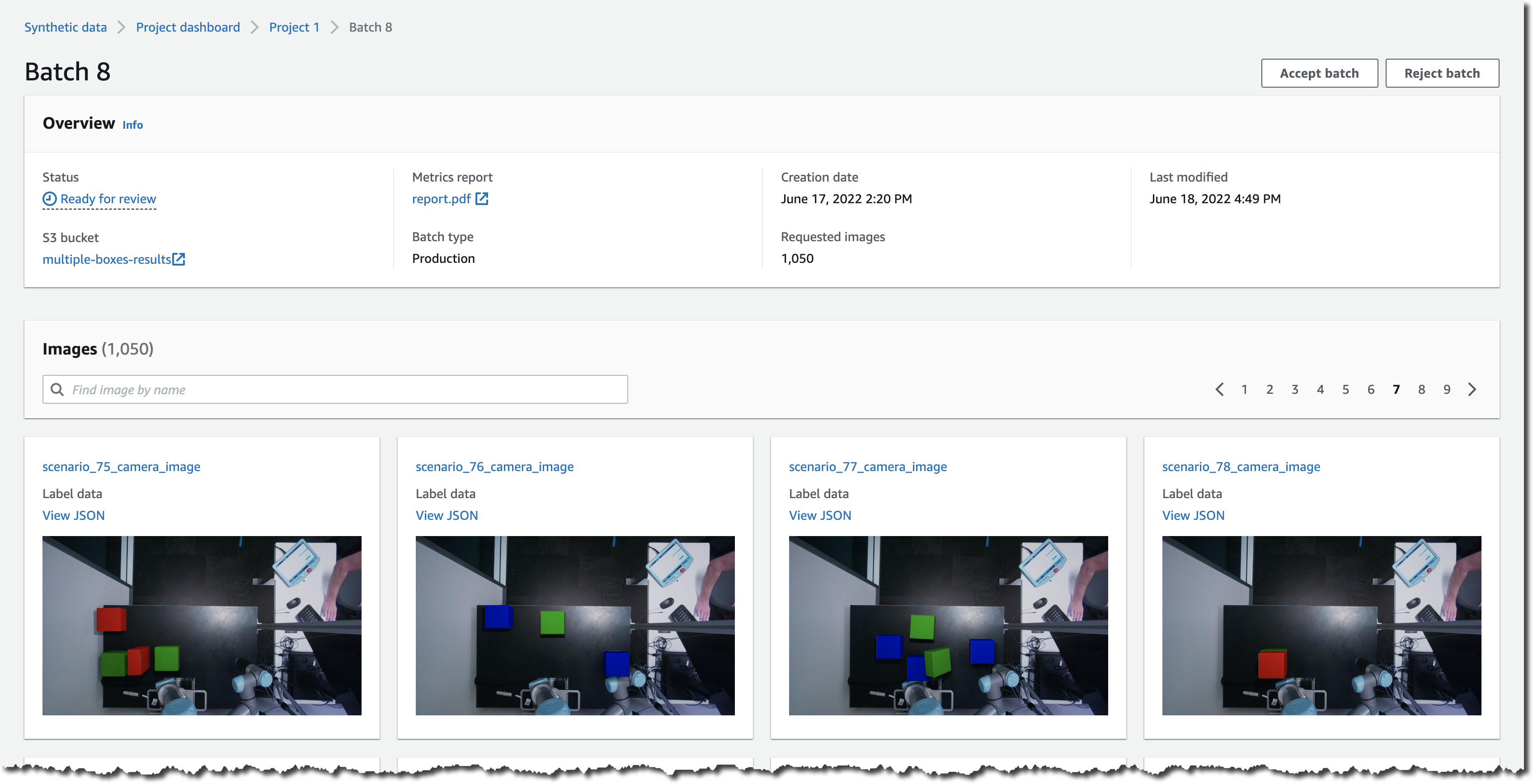
Select the batch you want to review and View details
Sample batch of synthetic data in Amazon SageMaker Ground Truth

In addition to the images, you will also receive output image labels, metadata such as object positions, and image quality metrics as Amazon SageMaker compatible JSON files.

Synthetic Image Fidelity and Diversity Report
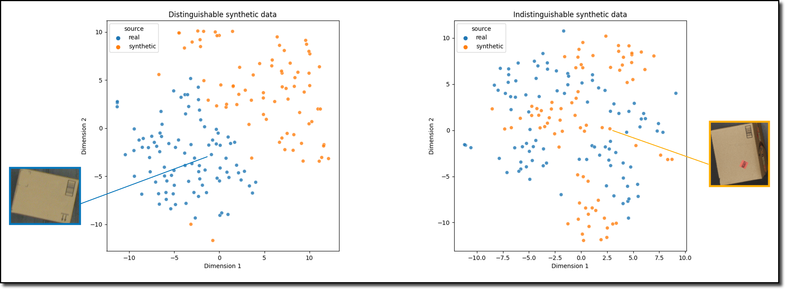
With each available batch of images, you also receive a synthetic image fidelity and diversity report. This report provides image and object level statistics and plots that help you make sense of the generated synthetic images.

The statistics are used to describe the diversity and the fidelity of the synthetic images and compare them with real images. Examples of the statistics and plots provided are the distributions of object classes, object sizes, image brightness, and image contrast, as well as the plots evaluating the indistinguishability between synthetic and real images.

Synthetic Image Fidelity and Diversity Report

Once you approve the pilot production test batch, the team will move to the production phase and start generating larger batches of labeled synthetic images with your desired label types, such as 2D bounding boxes, instance segmentation, and contours. Similar to the test batch, each production batch of images will be made available for you together with the image fidelity and diversity report to spot-check, accept, or reject.

All images and artifacts will be available for you to download from your S3 bucket once final production is complete.

Availability
Amazon SageMaker Ground Truth synthetic data is available in US East (N. Virginia). Synthetic data is priced on a per-label basis. You can request a custom quote that is tailored to your specific use case and requirements by filling out the project requirement form.

Learn more about SageMaker Ground Truth synthetic data on our Amazon SageMaker Data Labeling page.

Request your synthetic data project through the Amazon SageMaker Ground Truth console today!

— Antje

Use a linear learner algorithm in Amazon Redshift ML to solve regression and classification problems

Post Syndicated from Phil Bates original https://aws.amazon.com/blogs/big-data/use-a-linear-learner-algorithm-in-amazon-redshift-ml-to-solve-regression-and-classification-problems/

Amazon Redshift is the fastest, most widely used, fully managed, and petabyte-scale cloud data warehouse. Tens of thousands of customers use Amazon Redshift to process exabytes of data every day to power their analytics workloads. Amazon Redshift ML, powered by Amazon SageMaker, makes it easy for SQL users such as data analysts, data scientists, and database developers to create, train, and deploy machine learning (ML) models using familiar SQL commands and then use these models to make predictions on new data for use cases such as churn prediction, customer lifetime value prediction, and product recommendations. Redshift ML makes the model available as a SQL function within the Amazon Redshift data warehouse so you can easily use it in queries and reports. Customers across all verticals are using Redshift ML to derive better insights from their data. For example, Jobcase uses Redshift ML to recommend job search at scale. Magellan RX Management uses Redshift ML to predict drug therapeutic use conditions.

Amazon Redshift supports supervised learning, including regression, binary classification, multi-class classification, and unsupervised learning using K-Means. You can optionally specify XGBoost, MLP, and now linear learner model types, which are supervised learning algorithms used for solving either classification or regression problems, and provide a significant increase in speed over traditional hyperparameter optimization techniques. Amazon Redshift also supports bring-your-own-model to invoke remote SageMaker endpoints.

In this post, we show you how to use Redshift ML to solve regression and classification problems using the SageMaker linear learner algorithm, which explores different training objectives and chooses the best solution from a validation set.

Solution overview

We first solve a linear regression problem, followed by a multi-class classification problem.

The following table shows some common use cases and algorithms used.

Use Case Algorithm / Problem Type
Customer churn prediction Classification
Predict if a sales lead will close Classification
Fraud detection Classification
Price and revenue prediction Linear regression
Customer lifetime value prediction Linear regression

To use the linear learner algorithm, you need to provide inputs or columns representing dimensional values and also the label or target, which is the value you’re trying to predict. The linear learner algorithm trains many models in parallel, and automatically determines the most optimized model.

Prerequisites

To get started, we need an Amazon Redshift cluster or an Amazon Redshift Serverless endpoint and an AWS Identity and Access Management (IAM) role attached that provides access to SageMaker and permissions to an Amazon Simple Storage Service (Amazon S3) bucket.

For an introduction to Redshift ML and instructions on setting it up, see Create, train, and deploy machine learning models in Amazon Redshift using SQL with Amazon Redshift ML.

To create a simple cluster with a default IAM role, see Use the default IAM role in Amazon Redshift to simplify accessing other AWS services.

Use case 1: Linear regression

In this use case, we analyze the Abalone dataset and determine the relationship between the physical measurements and use that to determine the age of abalone. The age of abalone is determined by cutting the shell through the cone, staining it, and counting the number of rings through a microscope, which is a time-consuming task. We want to predict the age using different physical measurements, which is easier to measure. The age of abalone is (number of rings + 1.5) years.

Prepare the data

Load the Abalone dataset into Amazon Redshift using the following SQL. You can use the Amazon Redshift query editor v2 or your preferred SQL tool to run these commands.

To create the table, use the following commands:

create table abalone_dataset
( 
id INT IDENTITY(1,1),
Sex     CHAR(1),
Length float,
Diameter float,
Height float,
Whole  float,
Shucked  float,
Viscera  float,
Shell float,
Rings  integer   
); 

To load data into Amazon Redshift, use the following COPY command:

COPY abalone_dataset 
from 's3://redshift-ml-multiclass/abalone.csv' 
REGION 'us-east-1'
IAM_ROLE default
CSV IGNOREHEADER 1
NULL AS 'NULL'; 

To train the model, we use the abalone table and 80% of the data to train the model, and then test the accuracy of that model by seeing if it correctly predicts the age of ring label attribute on the remaining 20% of the data. Run the following command to create training and validation tables:

create table abalone_training as
  select * from abalone_dataset where mod(id,10) < 8 ; 

create table abalone_validation as
  select * from abalone_dataset where mod(id,10) >= 8; 

Create a model in Redshift ML

To create a model in Amazon Redshift, use the following command:

CREATE MODEL model_abalone_ring_prediction
FROM (
 SELECT   Sex ,
Length ,
Diameter ,
Height ,
Whole  ,
Shucked  ,
Viscera  ,
Shell,
Rings  as target_label
FROM abalone_training
) TARGET target_label
FUNCTION f_abalone_ring_prediction
IAM_ROLE default
MODEL_TYPE LINEAR_LEARNER 
PROBLEM_TYPE REGRESSION
OBJECTIVE 'MSE'
SETTINGS (
  S3_BUCKET '<your-s3-bucket>',
  MAX_RUNTIME 15000
  ); 

We define the following parameters in the CREATE MODEL statement:

  • Problem type – We use the linear learner problem type, which is newly added to extend upon typical linear models by training many models in parallel, in a computationally efficient manner.
  • Objective – We specified MSE (mean square error) as our objective, which is a common metric for evaluation of regression problems.
  • Max runtime –This parameter denotes how long the model training can run. Specifying a larger value may help create a better tuned model. The default value for this parameter is 5400 (90 minutes). For this example, we set it to 15000.

The preceding statement takes a few seconds to complete. It initiates an Amazon SageMaker Autopilot process in the background to automatically build, train, and tune the best ML model for the input data. It then uses Amazon SageMaker Neo to deploy that model locally in the Amazon Redshift cluster or Amazon Redshift Serverless as a user-defined function (UDF). You can use the SHOW MODEL command in Amazon Redshift to track the progress of your model creation, which should be in the READY state within the max_runtime parameter you defined while creating the model.

To check the status of the model, use the following command:

show model model_abalone_ring_prediction;

The following is the tabular outcome for the preceding command after model training was done. It took approximately 120 minutes to train the model.

Key Value
Model Name model_abalone_ring_prediction
Schema Name public
Owner awsuser
Creation Time Tue, 10.05.2022 19:42:33
Model State READY
validation:mse 4.082088
Estimated Cost 5.423719
. .
TRAINING DATA: .
Query SELECT SEX , LENGTH , DIAMETER , HEIGHT , WHOLE , SHUCKED , VISCERA , SHELL, RINGS AS TARGET_LABEL
. FROM ABALONE_TRAINING
Target Column TARGET_LABEL
. .
PARAMETERS: .
Model Type linear_learner
Problem Type Regression
Objective MSE
AutoML Job Name redshiftml-20220510194233380173
Function Name f_abalone_ring_prediction
Function Parameters sex length diameter height whole shucked viscera shell
Function Parameter Types bpchar float8 float8 float8 float8 float8 float8 float8
IAM Role default-aws-iam-role
S3 Bucket poc-generic-bkt
Max Runtime 15000

Model validation

We notice from the preceding table that the MSE for the training data is 4.08. Now let’s run the prediction query and validate the accuracy of the model on the testing and validation dataset:

select
ROUND(AVG(POWER(( tgt_label - predicted ),2)),2) mse
, ROUND(SQRT(AVG(POWER(( tgt_label - predicted ),2))),2) rmse
from 
(
SELECT   Sex ,
Length ,
Diameter ,
Height ,
Whole  ,
Shucked  ,
Viscera  ,
Shell,
Rings as tgt_label,
f_abalone_ring_prediction(Sex ,Length ,Diameter ,Height ,Whole  ,Shucked  ,Viscera  ,Shell) as predicted,
case when tgt_label = predicted then 1
      else 0 end as match,
  case when tgt_label  <> predicted then 1
    else 0 end as nonmatch
FROM abalone_validation
)t1 

The following is the outcome from the query:

mse rmse
5.08 2.25

The MSE value from the preceding query results indicates that our model is accurate enough to the actual values from our validation dataset.

We can also observe that Redshift ML is able to identify the right combination of features to come up with a usable prediction model. We can further check the impact of each attribute and its contribution and weightage in the model selection using the following command:

select explain_model ('model_abalone_ring_prediction')

The following is the outcome, where each attribute weightage is representative of its role in model decision-making:

{"explanations":
    {"kernel_shap":
      {"label0":
        {"expected_value":10.06938362121582,
          "global_shap_values":
          {
            "diameter":0.6897614190439705,
            "height":0.38391156156643987,
            "length":0.29646334630067408,
            "sex":0.5516722137411109,
            "shell":1.5679368167990147,
            "shucked":2.222549468867254,
            "viscera":0.2879883139361144,
            "whole":0.8085603201751219
            }
        }
       }
      }
      ,"version":"1.0"
    }

Use case 2: Multi-class classification

For this use case, we use the Covertype dataset (copyright Jock A. Blackard and Colorado State University), which contains information collected by the US Geological Survey and the US Forest Service about wilderness areas in northern Colorado. This has been downloaded to an S3 bucket to make it simple to create the model. You may want to download the dataset description. This dataset contains various measurements such as elevation, distance to waters and roadways, as well as the wilderness area designation and the soil type. Our ML task is to create a model to predict the cover type for a given area.

Prepare the data

To prepare the data for this model, you need to create and populate the table public.covertype_data in Amazon Redshift using the Covertype dataset. You may use the following SQL in Amazon Redshift query editor v2 or your preferred SQL tool:

CREATE TABLE public.covertype_data (
    elevation bigint ENCODE az64,
    aspect bigint ENCODE az64,
    slope bigint ENCODE az64,
    horizontal_distance_to_hydrology bigint ENCODE az64,
    vertical_distance_to_hydrology bigint ENCODE az64,
    horizontal_distance_to_roadways bigint ENCODE az64,
    hillshade_9am bigint ENCODE az64,
    hillshade_noon bigint ENCODE az64,
    hillshade_3pm bigint ENCODE az64,
    horizontal_distance_to_fire_points bigint ENCODE az64,
    wilderness_area1 bigint ENCODE az64,
    wilderness_area2 bigint ENCODE az64,
    wilderness_area3 bigint ENCODE az64,
    wilderness_area4 bigint ENCODE az64,
    soil_type1 bigint ENCODE az64,
    soil_type2 bigint ENCODE az64,
    soil_type3 bigint ENCODE az64,
    soil_type4 bigint ENCODE az64,
    soil_type5 bigint ENCODE az64,
    soil_type6 bigint ENCODE az64,
    soil_type7 bigint ENCODE az64,
    soil_type8 bigint ENCODE az64,
    soil_type9 bigint ENCODE az64,
    soil_type10 bigint ENCODE az64,
    soil_type11 bigint ENCODE az64,
    soil_type12 bigint ENCODE az64,
    soil_type13 bigint ENCODE az64,
    soil_type14 bigint ENCODE az64,
    soil_type15 bigint ENCODE az64,
    soil_type16 bigint ENCODE az64,
    soil_type17 bigint ENCODE az64,
    soil_type18 bigint ENCODE az64,
    soil_type19 bigint ENCODE az64,
    soil_type20 bigint ENCODE az64,
    soil_type21 bigint ENCODE az64,
    soil_type22 bigint ENCODE az64,
    soil_type23 bigint ENCODE az64,
    soil_type24 bigint ENCODE az64,
    soil_type25 bigint ENCODE az64,
    soil_type26 bigint ENCODE az64,
    soil_type27 bigint ENCODE az64,
    soil_type28 bigint ENCODE az64,
    soil_type29 bigint ENCODE az64,
    soil_type30 bigint ENCODE az64,
    soil_type31 bigint ENCODE az64,
    soil_type32 bigint ENCODE az64,
    soil_type33 bigint ENCODE az64,
    soil_type34 bigint ENCODE az64,
    soil_type35 bigint ENCODE az64,
    soil_type36 bigint ENCODE az64,
    soil_type37 bigint ENCODE az64,
    soil_type38 bigint ENCODE az64,
    soil_type39 bigint ENCODE az64,
    soil_type40 bigint ENCODE az64,
    cover_type bigint ENCODE az64 
)
DISTSTYLE AUTO;	


Copy public.covertype_data
From 's3://redshift-ml-multiclass/covtype.data.gz'
iam_role default 
gzip
delimiter ','
region 'us-east-1';

Now that our dataset is loaded, we run the following SQL statements to split the data into three sets for training (80%), validation (10%), and prediction (10%). Note that Redshift ML Autopilot automatically splits the data into training and validation, but by splitting it here, you’re able to verify the accuracy of your model.

To prepare the dataset, assign random values to split the data:

create table  public.covertype_data_prep  as
select a.*,
cast (random() * 80 as int) as data_group_id
from public.covertype_data a;

Use the following code for the training set:

Create table public.covertype_training as
Select * from public.covertype_data_prep
Where data_group_id < 80;

Use the following code for the validation set:

Create table public.covertype_validation as
Select * from public.covertype_data_prep
Where data_group_id between 80 and 89;

Use the following code for the test set:

Create table public.covertype_test as
Select * from public.covertype_data_prep
Where data_group_id > 89; 

Now that we have our datasets, it’s time to create the model.

Create a model in Redshift ML using linear learner

Run the following SQL command to create your model—note our target is cover_type and we use all the inputs from our training set:

CREATE  MODEL forest_cover_type_model
FROM (select Elevation, 
   Aspect,  
   Slope,  
   Horizontal_distance_to_hydrology,  
   Vertical_distance_to_hydrology,   
   Horizontal_distance_to_roadways,  
   HIllshade_9am,  
   Hillshade_noon,  
   Hillshade_3pm , 
   Horizontal_Distance_To_Fire_Points,  
   Wilderness_Area1,  
   Wilderness_Area2,   
   Wilderness_Area3,  
   Wilderness_Area4,  
   soil_type1,
   Soil_Type2,
   Soil_Type3, 
   Soil_Type4, 
   Soil_Type5,  
   Soil_Type6, 
   Soil_Type7,  
   Soil_Type8, 
   Soil_Type9, 
   Soil_Type10 , 
   Soil_Type11,  
   Soil_Type12 , 
   Soil_Type13 ,
   Soil_Type14, 
   Soil_Type15, 
   Soil_Type16,  
   Soil_Type17, 
   Soil_Type18,  
   Soil_Type19,  
   Soil_Type20,  
   Soil_Type21,  
   Soil_Type22,  
   Soil_Type23,  
   Soil_Type24, 
   Soil_Type25,  
   Soil_Type26, 
   Soil_Type27,  
   Soil_Type28,  
   Soil_Type29,  
   Soil_Type30,  
   Soil_Type31, 
   Soil_Type32, 
   Soil_Type33,  
   Soil_Type34, 
   Soil_Type36, 
   Soil_Type37,  
   Soil_Type38,  
   Soil_Type39, 
   Soil_Type40,
  Cover_type from public.covertype_training)
TARGET cover_type
FUNCTION predict_cover_type
IAM_ROLE default
MODEL_TYPE LINEAR_LEARNER              
PROBLEM_TYPE MULTICLASS_CLASSIFICATION 
 OBJECTIVE 'Accuracy'
SETTINGS (
  S3_BUCKET '<<your-amazon-s3-bucket-name>>’
, 
  S3_GARBAGE_COLLECT OFF,
  MAX_RUNTIME 9600
) ;

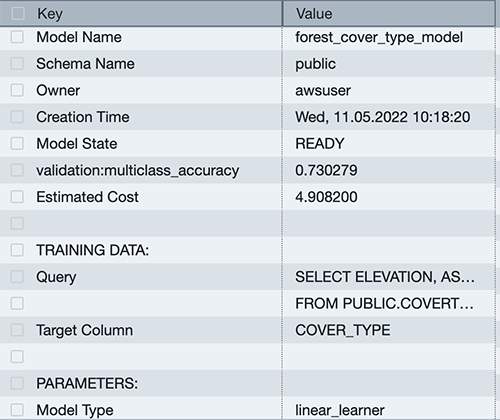
You can use the SHOW MODEL command to view the status of the model.

You can see that the model has an accuracy score of .730279 and is in the READY state. Now let’s run a query to do some validation of our own.

Model validation

Run the following SQL query against the validation table, using the function created by our model:

select 
 cast(sum(t1.match)as decimal(7,2)) as predicted_matches
,cast(sum(t1.nonmatch) as decimal(7,2)) as predicted_non_matches
,cast(sum(t1.match + t1.nonmatch) as decimal(7,2))  as total_predictions
,predicted_matches / total_predictions as pct_accuracy
from 
(select 
Elevation, 
   Aspect,  
   Slope,  
   Horizontal_distance_to_hydrology,  
   Vertical_distance_to_hydrology,   
   Horizontal_distance_to_roadways,  
   HIllshade_9am,  
   Hillshade_noon,  
   Hillshade_3pm , 
   Horizontal_Distance_To_Fire_Points,  
   Wilderness_Area1,  
   Wilderness_Area2,   
   Wilderness_Area3,  
   Wilderness_Area4,  
   soil_type1,
   Soil_Type2,
   Soil_Type3, 
   Soil_Type4, 
   Soil_Type5,  
   Soil_Type6, 
   Soil_Type7,  
   Soil_Type8, 
   Soil_Type9, 
   Soil_Type10 , 
   Soil_Type11,  
   Soil_Type12 , 
   Soil_Type13 ,
   Soil_Type14, 
   Soil_Type15, 
   Soil_Type16,  
   Soil_Type17, 
   Soil_Type18,  
   Soil_Type19,  
   Soil_Type20,  
   Soil_Type21,  
   Soil_Type22,  
   Soil_Type23,  
   Soil_Type24, 
   Soil_Type25,  
   Soil_Type26, 
   Soil_Type27,  
   Soil_Type28,  
   Soil_Type29,  
   Soil_Type30,  
   Soil_Type31, 
   Soil_Type32, 
   Soil_Type33,  
   Soil_Type34, 
   Soil_Type36, 
   Soil_Type37,  
   Soil_Type38,  
   Soil_Type39, 
   Soil_Type40,
   Cover_type as actual_cover_type,
   predict_cover_type( Elevation, 
   Aspect,  
   Slope,  
   Horizontal_distance_to_hydrology,  
   Vertical_distance_to_hydrology,   
   Horizontal_distance_to_roadways,  
   HIllshade_9am,  
   Hillshade_noon,  
   Hillshade_3pm , 
   Horizontal_Distance_To_Fire_Points,  
   Wilderness_Area1,  
   Wilderness_Area2,   
   Wilderness_Area3,  
   Wilderness_Area4,  
   soil_type1,
   Soil_Type2,
   Soil_Type3, 
   Soil_Type4, 
   Soil_Type5,  
   Soil_Type6, 
   Soil_Type7,  
   Soil_Type8, 
   Soil_Type9, 
   Soil_Type10 , 
   Soil_Type11,  
   Soil_Type12 , 
   Soil_Type13 ,
   Soil_Type14, 
   Soil_Type15, 
   Soil_Type16,  
   Soil_Type17, 
   Soil_Type18,  
   Soil_Type19,  
   Soil_Type20,  
   Soil_Type21,  
   Soil_Type22,  
   Soil_Type23,  
   Soil_Type24, 
   Soil_Type25,  
   Soil_Type26, 
   Soil_Type27,  
   Soil_Type28,  
   Soil_Type29,  
   Soil_Type30,  
   Soil_Type31, 
   Soil_Type32, 
   Soil_Type33,  
   Soil_Type34, 
   Soil_Type36, 
   Soil_Type37,  
   Soil_Type38,  
   Soil_Type39, 
   Soil_Type40) as predicted_cover_type,
case when actual_cover_type = predicted_cover_type then 1
      else 0 end as match,
  case when actual_cover_type <>  predicted_cover_type then 1
    else 0 end as nonmatch

from public.covertype_validation
) t1;

You can see that our accuracy is very close to our score from the SHOW MODEL output.

Run a prediction query

Let’s run a prediction query in Amazon Redshift ML using our function against our test dataset to see the most common class of cover type for the Neota Wilderness Area. We can denote this by checking wildnerness_area2 for a value of 1.

The dataset includes the following wilderness areas:

  1. Rawah Wilderness Area
  2. Neota Wilderness Area
  3. Comanche Peak Wilderness Area
  4. Cache la Poudre Wilderness Area

The cover types are in seven different classes:

  1. Spruce/Fir
  2. Lodgepole Pine
  3. Ponderosa Pine
  4. Cottonwood/Willow
  5. Aspen
  6. Douglas Fir
  7. Krummholz

There are also 40 different soil type definitions, which you can see in the dataset description, with a value of 0 or 1 to note if it’s applicable for a particular row. The following are a few example soil types:

  1. Cathedral family – Rock outcrop complex, extremely stony
  2. Vanet-Ratake families –Rocky outcrop complex, very stony
  3. Haploborolis family – Rock outcrop complex, rubbly
  4. Ratake family – Rock outcrop complex, rubbly
  5. Vanet family – Rock outcrop complex, rubbly
  6. Vanet-Wetmore families – Rock outcrop complex, stony
select t1. predicted_cover_type, count(*) 
from 
(     
select 
   Elevation, 
   Aspect,  
   Slope,  
   Horizontal_distance_to_hydrology,  
   Vertical_distance_to_hydrology,   
   Horizontal_distance_to_roadways,  
   HIllshade_9am,  
   Hillshade_noon,  
   Hillshade_3pm , 
   Horizontal_Distance_To_Fire_Points,  
   Wilderness_Area1,  
   Wilderness_Area2,   
   Wilderness_Area3,  
   Wilderness_Area4,  
   soil_type1,
   Soil_Type2,
   Soil_Type3, 
   Soil_Type4, 
   Soil_Type5,  
   Soil_Type6, 
   Soil_Type7,  
   Soil_Type8, 
   Soil_Type9, 
   Soil_Type10 , 
   Soil_Type11,  
   Soil_Type12 , 
   Soil_Type13 ,
   Soil_Type14, 
   Soil_Type15, 
   Soil_Type16,  
   Soil_Type17, 
   Soil_Type18,  
   Soil_Type19,  
   Soil_Type20,  
   Soil_Type21,  
   Soil_Type22,  
   Soil_Type23,  
   Soil_Type24, 
   Soil_Type25,  
   Soil_Type26, 
   Soil_Type27,  
   Soil_Type28,  
   Soil_Type29,  
   Soil_Type30,  
   Soil_Type31, 
   Soil_Type32, 
   Soil_Type33,  
   Soil_Type34, 
   Soil_Type36, 
   Soil_Type37,  
   Soil_Type38,  
   Soil_Type39, 
   Soil_Type40,
   predict_cover_type( Elevation, 
   Aspect,  
   Slope,  
   Horizontal_distance_to_hydrology,  
   Vertical_distance_to_hydrology,   
   Horizontal_distance_to_roadways,  
   HIllshade_9am,  
   Hillshade_noon,  
   Hillshade_3pm , 
   Horizontal_Distance_To_Fire_Points,  
   Wilderness_Area1,  
   Wilderness_Area2,   
   Wilderness_Area3,  
   Wilderness_Area4,  
   soil_type1,
   Soil_Type2,
   Soil_Type3, 
   Soil_Type4, 
   Soil_Type5,  
   Soil_Type6, 
   Soil_Type7,  
   Soil_Type8, 
   Soil_Type9, 
   Soil_Type10,
   Soil_Type11,  
   Soil_Type12, 
   Soil_Type13,
   Soil_Type14, 
   Soil_Type15, 
   Soil_Type16,  
   Soil_Type17, 
   Soil_Type18,  
   Soil_Type19,  
   Soil_Type20,  
   Soil_Type21,  
   Soil_Type22,  
   Soil_Type23,  
   Soil_Type24, 
   Soil_Type25,  
   Soil_Type26, 
   Soil_Type27,  
   Soil_Type28,  
   Soil_Type29,  
   Soil_Type30,  
   Soil_Type31, 
   Soil_Type32, 
   Soil_Type33,  
   Soil_Type34, 
   Soil_Type36, 
   Soil_Type37,  
   Soil_Type38,  
   Soil_Type39, 
   Soil_Type40) as predicted_cover_type 

from public.covertype_test
where wilderness_area2 = 1)
t1
group by 1;

Our model has predicted that the majority of cover is Spruce and Fir.

You can experiment with various combinations, such as determining which soil types are most likely to occur in a predicted cover type.

Conclusion

Redshift ML makes it easy for users of all levels to create, train, and tune models using a SQL interface. In this post, we walked you through how to use the linear learner algorithm to create regression and multi-class classification models. You can then use those models to make predictions using simple SQL commands and gain valuable insights.

To learn more about RedShift ML, visit Amazon Redshift ML.


About the Authors

Phil Bates is a Senior Analytics Specialist Solutions Architect at AWS with over 25 years of data warehouse experience.

Sohaib Katariwala is an Analytics Specialist Solutions Architect at AWS. He has 12+ years of experience helping organizations derive insights from their data.

Tahir Aziz is an Analytics Solution Architect at AWS. He has worked with building data warehouses and big data solutions for over 13 years. He loves to help customers design end-to-end analytics solutions on AWS. Outside of work, he enjoys traveling and cooking.

Jiayuan Chen is a Senior Software Development Engineer at AWS. He is passionate about designing and building data-intensive applications, and has been working in the areas of data lake, query engine, ingestion, and analytics. He keeps up with latest technologies and innovates things that spark joy.

Debu Panda is a Senior Manager, Product Management at AWS, is an industry leader in analytics, application platform, and database technologies, and has more than 25 years of experience in the IT world. Debu has published numerous articles on analytics, enterprise Java, and databases and has presented at multiple conferences such as re:Invent, Oracle Open World, and Java One. He is lead author of the EJB 3 in Action (Manning Publications 2007, 2014) and Middleware Management (Packt).

Detecting data drift using Amazon SageMaker

Post Syndicated from Shibu Nair original https://aws.amazon.com/blogs/architecture/detecting-data-drift-using-amazon-sagemaker/

As companies continue to embrace the cloud and digital transformation, they use historical data in order to identify trends and insights. This data is foundational to power tools, such as data analytics and machine learning (ML), in order to achieve high quality results.

This is a time where major disruptions are not only lasting longer, but also happening more frequently, as discussed in a McKinsey article on risk and resilience. Any disruption—a pandemic, hurricane, or even blocked sailing routes—has a major impact on the patterns of data and can create anomalous behavior.

ML models are dependent on data insights to help plan and support production-ready applications. With any disruptions, data drift can occur. Data drift is unexpected and undocumented changes to data structure, semantics, and/or infrastructure. If there is data drift, the model performance will degrade and no longer provide an accurate guidance. To mitigate the effects of the disruption, data drift needs to be detected and the ML models quickly trained and adjusted accordingly.
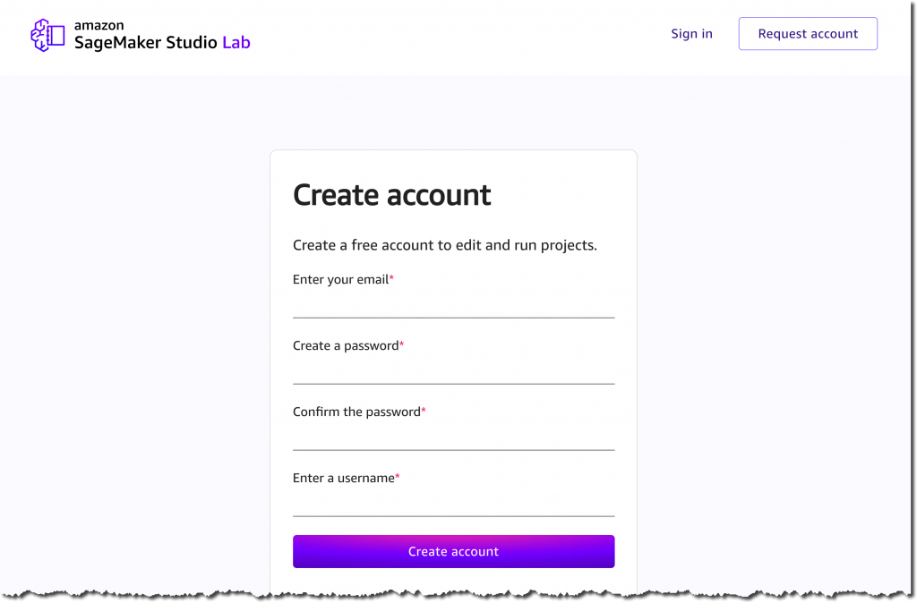
This blog post explains how to approach changing data patterns in the age of disruption and how to mitigate its effects on ML models. We also discuss the steps of building a feedback loop to capture the request data in the production environment and create a data pipeline to store the data for profiling and baselining. Then, we explain how Amazon SageMaker Clarify can help detect data drift.

How to detect data drift

There are three stages to detecting data drift: data quality monitoring, model quality monitoring, and drift evaluation (see Figure 1).

Stages in detecting data drift

Figure 1. Stages in detecting data drift

Data quality monitoring establishes a profile of the input data during model training, and then continuously compares incoming data with the profile. Deviations in the data profile signal a drift in the input data.

You can also detect drift through model quality monitoring, which requires capturing actual values that can be compared with the predictions. For example, using weekly demand forecasting, you can compare the forecast quantities one week later with the actual demand. Some use cases can require extra steps to collect actual values. For example, product recommendations may require you to ask a selected group of consumers for their feedback to the recommendation.

SageMaker Clarify provides insights into your trained models, including importance of model features and any biases towards certain segments of the input data. Changes of these attributes between re-trained models also signal drift. Drift evaluation constitutes the monitoring data and mechanisms to detect changes and triggering consequent actions. With Amazon CloudWatch, you can define rules and thresholds that prompt drift notifications.

Figure 2 illustrates a basic architecture with the data sources for training and production (on the left) and the observed data concerning drift (on the right). You can use Amazon SageMaker Data Wrangler, a visual data preparation tool, to clean and normalize your input data for your ML task. You can store the features that you defined for your models in the Amazon SageMaker Feature Store, a fully managed, purpose-built repository to store, update, retrieve, and share ML features.

The white, rectangular boxes in the architecture diagram represent the tasks for detecting data and model drift. You can integrate those tasks into your ML workflow with Amazon SageMaker Pipelines.

Basic architecture on how data drift is detected using Amazon SageMaker

Figure 2. Basic architecture on how data drift is detected using Amazon SageMaker

The drift observation data can be captured in tabular format, such as comma-separated values or Parquet, on Amazon Simple Storage Service (S3) and analyzed with Amazon Athena and Amazon QuickSight.

How to build a feedback loop

The baselining task establishes a data profile from training data. It uses Amazon SageMaker Model Monitor and runs before training or re-training the model. The baseline profile is stored on Amazon S3 to be referenced by the data drift monitoring job.

The data drift monitoring task continuously profiles the input data, compares it with baseline, and the results are captured in CloudWatch. This tasks runs on its own computation resources using Deequ, which checks that the monitoring job does not slow down your ML inference flow and scales with the data. The frequency of running this task can be adjusted to control cost, which can depend on how rapidly you anticipate that the data may change.

The model quality monitoring task computes model performance metrics from actuals and predicted values. The origin of these data points depends on the use case. Demand forecasting use cases naturally capture actuals that can be used to validate past predictions. Other use cases can require extra steps to acquire ground-truth data.

CloudWatch is a monitoring and observability service with which you can define rules to act on deviation in model performance or data drift. With CloudWatch, you can setup alerts to users via e-mail or SMS, and it can automatically start the ML model re-training process.

Run the baseline task on your updated data set before re-training your model. Use the SageMaker model registry to catalog your ML models for production, manage model versions, and control the associate training metrics.

Gaining insight into data and models

SageMaker Clarify provides greater visibility into your training data and models, helping identify and limit bias and explain predictions. For example, the trained models may consider some features more strongly than others when generating predictions. Compare the feature importance and bias between model-provided versions for a better understanding of the changes.

Conclusion

As companies continue to use data analytics and ML to inform daily activity, data drift may become a more common occurrence. Recognizing that drift can have a direct impact on models and production-ready applications, it is important to architect to identify potential data drift and avoid downgrading the models and negatively impacting results. Failure to capture changes in data can result in loss of process confidence, downgraded model accuracy, or a bottom-line impact to the business.

Secure data movement across Amazon S3 and Amazon Redshift using role chaining and ASSUMEROLE

Post Syndicated from Sudipta Mitra original https://aws.amazon.com/blogs/big-data/secure-data-movement-across-amazon-s3-and-amazon-redshift-using-role-chaining-and-assumerole/

Data lakes use a ring of purpose-built data services around a central data lake. Data needs to move between these services and data stores easily and securely. The following are some examples of such services:

  • Amazon Simple Storage Service (Amazon S3), which stores structured, unstructured, and semi-structured data
  • Amazon Redshift, a fully managed, petabyte-scale data warehouse product to analyze large-scale structured and semi-structured data across data warehouses and operational databases
  • Amazon SageMaker, which consumes data for machine learning (ML) capabilities

In multi-tenant architectures, groups or users within a group may require exclusive permissions to the group’s S3 bucket and also the schema and tables belonging to Amazon Redshift. These teams also need to be able to control loading and unloading of data between the team-owned S3 buckets and Amazon Redshift schemas. Additionally, individual users within the team may require fine-grained control over objects in S3 buckets and specific schemas in Amazon Redshift. Implementing this permissions control use case should be scalable as more teams and users are onboarded and permission-separation requirements evolve.

Amazon Redshift and Amazon S3 provide a unified, natively integrated storage layer for data lakes. You can move data between Amazon Redshift and Amazon S3 using the Amazon Redshift COPY and UNLOAD commands.

This post presents an approach that you can apply at scale to achieve fine-grained access controls to resources in S3 buckets and Amazon Redshift schemas for tenants, including groups of users belonging to the same business unit down to the individual user level. This solution provides tenant isolation and data security. In this approach, we use the bridge model to store data and control access for each tenant at the individual schema level in the same Amazon Redshift database. We utilize ASSUMEROLE and role chaining to provide fine-grained access control when data is being copied and unloaded between Amazon Redshift and Amazon S3, so the data flows within each tenant’s namespace. Role chaining also streamlines the new tenant onboarding process.

Solution overview

In this post, we explore how to achieve resource isolation, data security, scaling to multiple tenants, and fine-grained access control at the individual user level for teams that access, store, and move data across storage using Amazon S3 and Amazon Redshift.

We use the bridge model to store data and control access for each tenant at the individual schema level in the same Amazon Redshift database. In the bridge model, a separate database schema is created for each tenant, and data for each tenant is stored in its own schema. The tenant has access only to its own schema.

We use the COPY and UNLOAD commands to load and unload data into the Amazon Redshift cluster using an S3 bucket. These commands require Amazon Redshift to access Amazon S3 on your behalf, and security credentials are provided to your clusters.

We create an AWS Identity and Access Management (IAM) role—we call it the Amazon Redshift onboarding role—and associate it with the Amazon Redshift cluster. For each tenant, we create a tenant-specific IAM role—we call it the tenant role—to define the fine-grained access to its own Amazon S3 resources. The Amazon Redshift onboarding role doesn’t have any permissions granted except allowing sts:AssumeRole to the tenant roles. The trust relationship to the Amazon Redshift onboarding role is defined in each of the tenant roles. We use the Amazon Redshift ASSUMEROLE privilege to control IAM role access privileges for database users and groups on COPY and UNLOAD commands.

Each tenant database user or group is granted ASSUMEROLE on the Amazon Redshift onboarding role and its own tenant role, which restricts the tenant to access its own Amazon S3 resources when using COPY and UNLOAD commands. We use role chaining when ASSUMEROLE is granted. This means that the tenant role isn’t required to be attached to the Amazon Redshift cluster, and the only IAM role associated is the Amazon Redshift onboarding role. Role chaining streamlines the new tenant onboarding process. With role chaining, we don’t need to modify the cluster; we can make modifications on the tenant IAM role definition when onboarding a new tenant.

For our use case, we have two tenants: team 1 and team 2. A tenant here represents a group of users—a team from the same business unit. We want separate S3 buckets and Amazon Redshift schemas for each team. These teams should be able to access their own data only and also be able to support fine-grained access control over copying and unloading data from Amazon S3 to Amazon Redshift (and vice versa) within the team boundary. We can apply access control at the individual user level using the same approach.

The following architecture diagram shows the AWS resources and process flow of our solution.

In this tutorial, you create two S3 buckets, two Amazon Redshift tenant schemas, two Amazon Redshift tenant groups, one Amazon Redshift onboarding role, and two tenant roles. Then you grant ASSUMEROLE on the onboarding and tenant role to each tenant, using role chaining. To verify that each tenant can only access its own S3 resources, you create two Amazon Redshift users assigned to their own tenant group and run COPY and UNLOAD commands.

Prerequisites

To follow along with this solution, you need the following prerequisites:

Download the source code to your local environment

To implement this solution in your local development environment, you can download the source code from the GitHub repo or clone the source code using the following command:

git clone https://github.com/aws-samples/amazon-redshift-assume-role-sample.git

The following files are included in the source code:

  • redshift-onboarding-role.cf.yaml – A CloudFormation template to deploy the Amazon Redshift onboarding role redshift-onboarding-role
  • redshift-tenant-resources.cf.yaml – A CloudFormation template to deploy an S3 bucket, KMS key, and IAM role for each tenant you want to onboard

Provision an IAM role for Amazon Redshift and attach this role to the Amazon Redshift cluster

Deploy the template redshift-onboarding-role.cf.yaml using the AWS CloudFormation console or the AWS Command Line Interface (AWS CLI). For more information about stack creation, see Create the stack. This template doesn’t have any required parameters. The stack provisions an IAM role named redshift-s3-onboarding-role for Amazon Redshift. The following code is the policy defining sts:AssumeRole to the tenant-specific IAM roles:

{
  "Version": "2012-10-17",
  "Statement": [
  {
   "Action": [
     "sts:AssumeRole"
    ],
   "Resource": [
     "arn:aws:iam::xxxxxxxxxxxx:role/*-tenant-redshift-s3-access-role"
    ],
   "Effect": "Allow"
   }
  ]
}

Navigate to the Amazon Redshift console and select the cluster you want to update. On the Actions menu, choose Manage IAM roles. Choose the role redshift-s3-onboarding-role to associate with the cluster. For more information, see Associate the IAM role with your cluster.

Provision the IAM role and resources for tenants

Deploy the template redshift-tenant-resources.cf.yaml using the AWS CloudFormation console or the AWS CLI. For this post, you deploy the stack twice, supplying two unique tenant names for TenantName. For example, you can use team1 and team2 as the TenantName parameter values.

For each tenant, the stack provisions the following resources:

  • A KMS key
  • An S3 bucket named team1-data-<account id>-<region> with default encryption enabled with SSE-KMS using the created key
  • An IAM role named team1-tenant-redshift-s3-access-role

The policy attached to the role team1-tenant-redshift-s3-access-role can only access the team’s own S3 bucket. The role redshift-s3-onboarding-role is trusted to assume all tenant roles *-tenant-redshift-s3-access-role to enable role chaining. The tenant role *-tenant-redshift-s3-access-role has a trust relationship to redshift-s3-onboarding-role. See the following policy code:

        {
            "Action": [
                "s3:List*",
                "s3:Get*",
                "s3:Put*"
            ],
            "Resource": [
                "arn:aws:s3:::team1-data-<account id>-<region>/*",
                "arn:aws:s3:::team1-data-<account id>-<region>"
            ],
            "Effect": "Allow"
        }

Create a tenant schema and tenant user with appropriate privileges

For this post, you create the following Amazon Redshift database objects using the query editor on the Amazon Redshift console or a SQL client tool like SQL Workbench/J. Replace <password> with your password and <account id> with your AWS account ID before running the following SQL statements:

create schema team1;
create schema team2;

create group team1_grp;
create group team2_grp;

create user team1_usr with password '<password>' in group team1_grp;
create user team2_usr with password '<password>' in group team2_grp;

grant usage on schema team1 to group team1_grp;
grant usage on schema team2 to group team2_grp;

GRANT ALL ON SCHEMA team1 TO group team1_grp;
GRANT ALL ON SCHEMA team2 TO group team2_grp;

revoke assumerole on all from public for all;

grant assumerole
on 'arn:aws:iam::<account id>:role/redshift-s3-onboarding-role,arn:aws:iam::<account-id>:role/team1-tenant-redshift-s3-access-role'
to group team1_grp for copy;

grant assumerole
on 'arn:aws:iam::<account id>:role/redshift-s3-onboarding-role,arn:aws:iam::<account id>:role/team1-tenant-redshift-s3-access-role'
to group team1_grp for unload;

grant assumerole
on 'arn:aws:iam::<account id>:role/redshift-s3-onboarding-role,arn:aws:iam::<account id>:role/team2-tenant-redshift-s3-access-role'
to group team2_grp for copy;

grant assumerole
on 'arn:aws:iam::<account id>:role/redshift-s3-onboarding-role,arn:aws:iam::<account id>:role/team2-tenant-redshift-s3-access-role'
to group team2_grp for unload;

commit;

Verify that each tenant can only access its own resources

To verify your access control settings, you can create a test table in each tenant schema and upload a file to the tenant’s S3 bucket using the following commands. You can use the Amazon Redshift query editor or a SQL client tool.

  1. Sign in as team1_usr and enter the following commands:
    CREATE TABLE TEAM1.TEAM1_VENUE(
    VENUEID SMALLINT,
    VENUENAME VARCHAR(100),
    VENUECITY VARCHAR(30),
    VENUESTATE CHAR(2),
    VENUESEATS INTEGER
    ) DISTSTYLE EVEN;
    
    commit;

  2. Sign in as team2_usr and enter the following commands:
    CREATE TABLE TEAM2.TEAM2_VENUE(
    VENUEID SMALLINT,
    VENUENAME VARCHAR(100),
    VENUECITY VARCHAR(30),
    VENUESTATE CHAR(2),
    VENUESEATS INTEGER
    ) DISTSTYLE EVEN;
    
    commit;

  3. Create a file named test-venue.txt with the following contents:
    7|BMO Field|Toronto|ON|0
    16|TD Garden|Boston|MA|0
    23|The Palace of Auburn Hills|Auburn Hills|MI|0
    28|American Airlines Arena|Miami|FL|0
    37|Staples Center|Los Angeles|CA|0
    42|FedExForum|Memphis|TN|0
    52|PNC Arena|Raleigh|NC|0
    59|Scotiabank Saddledome|Calgary|AB|0
    66|SAP Center|San Jose|CA|0
    73|Heinz Field|Pittsburgh|PA|65050

  4. Upload this file to both team1 and team2 S3 buckets.
  5. Sign in as team1_usr and enter the following commands to test Amazon Redshift COPY and UNLOAD:
    copy team1.team1_venue
    from 's3://team1-data-<account id>-<region>/'
    iam_role 'arn:aws:iam::<account id>:role/redshift-s3-onboarding-role,arn:aws:iam::<account id>:role/team1-tenant-redshift-s3-access-role'
    delimiter '|' ;
    
    unload ('select * from team1.team1_venue')
    to 's3://team1-data-<account id>-<region>/unload/' 
    iam_role 'arn:aws:iam::<account id>:role/redshift-s3-onboarding-role,arn:aws:iam::<account id>:role/team1-tenant-redshift-s3-access-role';

The file test-venue.txt uploaded to the team1 bucket is copied to the table team1_venue in the team1 schema, and the data in table team1_venue is unloaded to the team1 bucket successfully.

  1. Replace team1 with team2 in the preceding commands and then run them again, this time signed in as team2_usr.

If you’re signed in as team1_usr and try to access the team2 S3 bucket or team2 schema or table and team2 IAM role when running COPY and UNLOAD, you get an access denied error. You get the same error if trying to access team1 resources while logged in as team2_usr.

Clean up

To clean up the resources you created, delete the CloudFormation stack created in your AWS account.

Conclusion

In this post, we presented a solution to achieve role-based secure data movement between Amazon S3 and Amazon Redshift. This approach combines with the ASSUMEROLE feature in Amazon Redshift to allow fine-grained access control over the COPY and UNLOAD commands down to the individual user level within a particular team. This in turn provides finer control over resource isolation and data security in a multi-tenant solution. Many use cases can benefit from this solution as more enterprises build data platforms to provide the foundations for highly scalable, customizable, and secure data consumption models.


About the Authors

Sudipta Mitra is a Senior Data Architect for AWS, and passionate about helping customers to build modern data analytics applications by making innovative use of latest AWS services and their constantly evolving features. A pragmatic architect who works backwards from customer needs, making them comfortable with the proposed solution, helping achieve tangible business outcomes. His main areas of work are Data Mesh, Data Lake, Knowledge Graph, Data Security and Data Governance.

Michelle Deng is a Sr. Data Architect at Amazon Web Services. She works with AWS customers to provide guidance and technical assistance about database migrations and Big data projects.

Jared Cook is a Sr. Cloud Infrastructure Architect at Amazon Web Services. He is committed to driving business outcomes in the cloud, and uses Infrastructure as Code and DevOps best practices to build resilient architectures on AWS.  In his leisure time, Jared enjoys the outdoors, music, and plays the drums.

Lisa Matacotta is a Senior Customer Solutions Manager at Amazon Web Services. She works with AWS customers to help customers achieve business and strategic goals, understand their biggest challenges and provide guidance based on AWS best practices to overcome them.

Amazon SageMaker Serverless Inference – Machine Learning Inference without Worrying about Servers

Post Syndicated from Antje Barth original https://aws.amazon.com/blogs/aws/amazon-sagemaker-serverless-inference-machine-learning-inference-without-worrying-about-servers/

In December 2021, we introduced Amazon SageMaker Serverless Inference (in preview) as a new option in Amazon SageMaker to deploy machine learning (ML) models for inference without having to configure or manage the underlying infrastructure. Today, I’m happy to announce that Amazon SageMaker Serverless Inference is now generally available (GA).

Different ML inference use cases pose different requirements on your model hosting infrastructure. If you work on use cases such as ad serving, fraud detection, or personalized product recommendations, you are most likely looking for API-based, online inference with response times as low as a few milliseconds. If you work with large ML models, such as in computer vision (CV) applications, you might require infrastructure that is optimized to run inference on larger payload sizes in minutes. If you want to run predictions on an entire dataset, or larger batches of data, you might want to run an on-demand, one-time batch inference job instead of hosting a model-serving endpoint. And what if you have an application with intermittent traffic patterns, such as a chatbot service or an application to process forms or analyze data from documents? In this case, you might want an online inference option that is able to automatically provision and scale compute capacity based on the volume of inference requests. And during idle time, it should be able to turn off compute capacity completely so that you are not charged.

Amazon SageMaker, our fully managed ML service, offers different model inference options to support all of those use cases:

Amazon SageMaker Serverless Inference in More Detail
In a lot of conversations with ML practitioners, I’ve picked up the ask for a fully managed ML inference option that lets you focus on developing the inference code while managing all things infrastructure for you. SageMaker Serverless Inference now delivers this ease of deployment.

Based on the volume of inference requests your model receives, SageMaker Serverless Inference automatically provisions, scales, and turns off compute capacity. As a result, you pay for only the compute time to run your inference code and the amount of data processed, not for idle time.

You can use SageMaker’s built-in algorithms and ML framework-serving containers to deploy your model to a serverless inference endpoint or choose to bring your own container. If traffic becomes predictable and stable, you can easily update from a serverless inference endpoint to a SageMaker real-time endpoint without the need to make changes to your container image. Using Serverless Inference, you also benefit from SageMaker’s features, including built-in metrics such as invocation count, faults, latency, host metrics, and errors in Amazon CloudWatch.

Since its preview launch, SageMaker Serverless Inference has added support for the SageMaker Python SDK and model registry. SageMaker Python SDK is an open-source library for building and deploying ML models on SageMaker. SageMaker model registry lets you catalog, version, and deploy models to production.

New for the GA launch, SageMaker Serverless Inference has increased the maximum concurrent invocations per endpoint limit to 200 (from 50 during preview), allowing you to use Amazon SageMaker Serverless Inference for high-traffic workloads. Amazon SageMaker Serverless Inference is now available in all the AWS Regions where Amazon SageMaker is available, except for the AWS GovCloud (US) and AWS China Regions.

Several customers have already started enjoying the benefits of SageMaker Serverless Inference:

Bazaarvoice leverages machine learning to moderate user-generated content to enable a seamless shopping experience for our clients in a timely and trustworthy manner. Operating at a global scale over a diverse client base, however, requires a large variety of models, many of which are either infrequently used or need to scale quickly due to significant bursts in content. Amazon SageMaker Serverless Inference provides the best of both worlds: it scales quickly and seamlessly during bursts in content and reduces costs for infrequently used models.” — Lou Kratz, PhD, Principal Research Engineer, Bazaarvoice

Transformers have changed machine learning, and Hugging Face has been driving their adoption across companies, starting with natural language processing and now with audio and computer vision. The new frontier for machine learning teams across the world is to deploy large and powerful models in a cost-effective manner. We tested Amazon SageMaker Serverless Inference and were able to significantly reduce costs for intermittent traffic workloads while abstracting the infrastructure. We’ve enabled Hugging Face models to work out of the box with SageMaker Serverless Inference, helping customers reduce their machine learning costs even further.” — Jeff Boudier, Director of Product, Hugging Face

Now, let’s see how you can get started on SageMaker Serverless Inference.

For this demo, I’ve built a text classifier to turn e-commerce customer reviews, such as “I love this product!” into positive (1), neutral (0), and negative (-1) sentiments. I’ve used the Women’s E-Commerce Clothing Reviews dataset to fine-tune a RoBERTa model from the Hugging Face Transformers library and model hub. I will now show you how to deploy the trained model to an Amazon SageMaker Serverless Inference Endpoint.

Deploy Model to an Amazon SageMaker Serverless Inference Endpoint
You can create, update, describe, and delete a serverless inference endpoint using the SageMaker console, the AWS SDKs, the SageMaker Python SDK, the AWS CLI, or AWS CloudFormation. In this first example, I will use the SageMaker Python SDK as it simplifies the model deployment workflow through its abstractions. You can also use the SageMaker Python SDK to invoke the endpoint by passing the payload in line with the request. I will show you this in a bit.

First, let’s create the endpoint configuration with the desired serverless configuration. You can specify the memory size and maximum number of concurrent invocations. SageMaker Serverless Inference auto-assigns compute resources proportional to the memory you select. If you choose a larger memory size, your container has access to more vCPUs. As a general rule of thumb, the memory size should be at least as large as your model size. The memory sizes you can choose are 1024 MB, 2048 MB, 3072 MB, 4096 MB, 5120 MB, and 6144 MB. For my RoBERTa model, let’s configure a memory size of 5120 MB and a maximum of five concurrent invocations.

import sagemaker
from sagemaker.serverless import ServerlessInferenceConfig

serverless_config = ServerlessInferenceConfig(
	memory_size_in_mb=5120, 
	max_concurrency=5
)

Now let’s deploy the model. You can use the estimator.deploy() method to deploy the model directly from the SageMaker training estimator, together with the serverless inference endpoint configuration. I also provide my custom inference code in this example.


endpoint_name="roberta-womens-clothing-serverless-1"

estimator.deploy(
	endpoint_name = endpoint_name, 
	entry_point="inference.py",
	serverless_inference_config=serverless_config
)

SageMaker Serverless Inference also supports model registry when you use the AWS SDK for Python (Boto3). I will show you how to deploy the model from the model registry later in this post.

Let’s check the serverless inference endpoint settings and deployment status. Go to the SageMaker console and browse to the deployed inference endpoint:

Review Amazon SageMaker Serverless Endpoint configuration in the SageMaker Console

From the SageMaker console, you can also create, update, or delete serverless inference endpoints if needed. In Amazon SageMaker Studio, select the endpoint tab and your serverless inference endpoint to review the endpoint configuration details.

Review Amazon SageMaker Serverless Endpoint configuration in SageMaker Studio

Once the endpoint status shows InService, you can start sending inference requests.

Now, let’s run a few sample predictions. My fine-tuned RoBERTa model expects the inference requests in JSON Lines format with the review text to classify as the input feature. A JSON Lines text file comprises several lines where each individual line is a valid JSON object, delimited by a newline character. This is an ideal format for storing data that is processed one record at a time, such as in model inference. You can learn more about JSON Lines and other common data formats for inference in the Amazon SageMaker Developer Guide. Note that the following code might look different depending on your model’s accepted inference request format.


from sagemaker.predictor import Predictor
from sagemaker.serializers import JSONLinesSerializer
from sagemaker.deserializers import JSONLinesDeserializer

sess = sagemaker.Session(sagemaker_client=sm)

inputs = [
    {"features": ["I love this product!"]},
    {"features": ["OK, but not great."]},
    {"features": ["This is not the right product."]},
]

predictor = Predictor(
    endpoint_name=endpoint_name,
    serializer=JSONLinesSerializer(),
    deserializer=JSONLinesDeserializer(),
    sagemaker_session=sess
)

predicted_classes = predictor.predict(inputs)

for predicted_class in predicted_classes:
    print("Predicted class {} with probability {}".format(predicted_class['predicted_label'], predicted_class['probability']))

The result will look similar to this, classifying the sample reviews into the corresponding sentiment classes.


Predicted class 1 with probability 0.9495596289634705
Predicted class 0 with probability 0.5395089387893677
Predicted class -1 with probability 0.7887083292007446

You can also deploy your model from the model registry to a SageMaker Serverless Inference endpoint. This is currently only supported through the AWS SDK for Python (Boto3). Let me walk you through another quick demo.

Deploy Model from the SageMaker Model Registry
To deploy the model from the model registry using Boto3, let’s first create a model object from the model version by calling the create_model() method. Then, I pass the Amazon Resource Name (ARN) of the model version as part of the containers for the model object.

import boto3
import sagemaker

sm = boto3.client(service_name='sagemaker')
role = sagemaker.get_execution_role()
model_name="roberta-womens-clothing-serverless"

container_list = 
	[{'ModelPackageName': <MODEL_PACKAGE_ARN>}]

create_model_response = sm.create_model(
    ModelName = model_name,
    ExecutionRoleArn = role,
    Containers = container_list
)

Next, I create the serverless inference endpoint. Remember that you can create, update, describe, and delete a serverless inference endpoint using the SageMaker console, the AWS SDKs, the SageMaker Python SDK, the AWS CLI, or AWS CloudFormation. For consistency, I keep using Boto3 in this second example.

Similar to the first example, I start by creating the endpoint configuration with the desired serverless configuration. I specify the memory size of 5120 MB and a maximum number of five concurrent invocations for my endpoint.

endpoint_config_name="roberta-womens-clothing-serverless-ep-config"

create_endpoint_config_response = sm.create_endpoint_config(
    EndpointConfigName = endpoint_config_name,
    ProductionVariants=[{
        'ServerlessConfig':{
            'MemorySizeInMB' : 5120,
            'MaxConcurrency' : 5
        },
        'ModelName':model_name,
        'VariantName':'AllTraffic'}])

Next, I create the SageMaker Serverless Inference endpoint by calling the create_endpoint() method.


endpoint_name="roberta-womens-clothing-serverless-2"

create_endpoint_response = sm.create_endpoint(
    EndpointName=endpoint_name,
    EndpointConfigName=endpoint_config_name)

Once the endpoint status shows InService, you can start sending inference requests. Again, for consistency, I choose to run the sample prediction using Boto3 and the SageMaker runtime client invoke_endpoint() method.

sm_runtime = boto3.client("sagemaker-runtime")
response = sm_runtime.invoke_endpoint(
    EndpointName=endpoint_name,
    ContentType="application/jsonlines",
    Accept="application/jsonlines",
    Body=bytes('{"features": ["I love this product!"]}', 'utf-8')
)

print(response['Body'].read().decode('utf-8'))
{"probability": 0.966135561466217, "predicted_label": 1}

How to Optimize Your Model for SageMaker Serverless Inference
SageMaker Serverless Inference automatically scales the underlying compute resources to process requests. If the endpoint does not receive traffic for a while, it scales down the compute resources. If the endpoint suddenly receives new requests, you might notice that it takes some time for the endpoint to scale up the compute resources to process the requests.

This cold-start time greatly depends on your model size and the start-up time of your container. To optimize cold-start times, you can try to minimize the size of your model, for example, by applying techniques such as knowledge distillation, quantization, or model pruning.

Knowledge distillation uses a larger model (the teacher model) to train smaller models (student models) to solve the same task. Quantization reduces the precision of the numbers representing your model parameters from 32-bit floating-point numbers down to either 16-bit floating-point or 8-bit integers. Model pruning removes redundant model parameters that contribute little to the training process.

Availability and Pricing
Amazon SageMaker Serverless Inference is now available in all the AWS Regions where Amazon SageMaker is available except for the AWS GovCloud (US) and AWS China Regions.

With SageMaker Serverless Inference, you only pay for the compute capacity used to process inference requests, billed by the millisecond, and the amount of data processed. The compute capacity charge also depends on the memory configuration you choose. For detailed pricing information, visit the SageMaker pricing page.

Get Started Today with Amazon SageMaker Serverless Inference
To learn more about Amazon SageMaker Serverless Inference, visit the Amazon SageMaker machine learning inference webpage. Here are SageMaker Serverless Inference example notebooks that will help you get started right away. Give them a try from the SageMaker console, and let us know what you think.

Antje

Backtest trading strategies with Amazon Kinesis Data Streams long-term retention and Amazon SageMaker

Post Syndicated from Sachin Thakkar original https://aws.amazon.com/blogs/big-data/backtest-trading-strategies-with-amazon-kinesis-data-streams-long-term-retention-and-amazon-sagemaker/

Real-time insight is critical when it comes to building trading strategies. Any delay in data insight can cost lot of money to the traders. Often, you need to look at historical market trends to predict future trading pattern and make the right bid. More the historical data you analyze, better trading prediction you get. Back tracking streaming data can be tricky as it requires sophisticated storage and analysis mechanisms.

Amazon Kinesis Data Streams allows our customer to store streaming data for up to one year. Amazon Kinesis Data Streams Long Term Retention (LTR) of streaming data enables to use the same platform for both real-time and older data retained in Amazon Kinesis Data Streams. For example, one can train machine learning algorithms for financial trading, marketing personalization, and recommendation models without moving the data into a different data store or writing a new application. Customers can also satisfy certain data retention regulations, including under HIPAA and FedRAMP, using long term retention. This thus simplifies the data ingestion architecture for our trading use case we will discuss in this post.

In the post Building algorithmic trading strategies with Amazon SageMaker, we demonstrated how to backtest trading strategies with Amazon SageMaker with historical stock price data stored in Amazon Simple Storage Service (Amazon S3). In this post, we expand this solution for streaming data and describe how to use Amazon Kinesis.

In addition, we want to use Amazon SageMaker automatic tuning to find the optimal configuration for a moving average crossover strategy. In this strategy, two moving averages for a slow and a fast time period are calculated, and a trade is executed when a crossover happens. If the fast moving average crosses above the slow moving average, the strategy places a long trade, otherwise the strategy goes short. We find the optimal period length for these moving averages by running multiple backtests with different lengths over a historical dataset.

Finally, we run the optimal configuration for this moving average crossover strategy over a different test dataset and analyze the performance results. If the performance measured in profit and loss (P&L) is positive for the test period, we can consider this trading strategy for a forward test.

To show you how easy and quick it is to get started on AWS, we provide a one-click deployment for an extensible trading backtesting solution that uses Kinesis long-term retention for streaming data.

Solution overview

We use Kinesis Data Streams to store real-time streaming as well as historical market data. We use Jupyter notebooks as our central interface for exploring and backtesting new trading strategies. SageMaker allows you to set up Jupyter notebooks and integrate them with AWS CodeCommit to store different versions of strategies and share them with other team members.

We use Amazon S3 to store model artifacts and backtesting results.

For our trading strategies, we create Docker containers that contain the required libraries for backtesting and the strategy itself. These containers follow the SageMaker Docker container structure in order to run them inside of SageMaker. For more information about the structure of SageMaker containers, see Using the SageMaker Training and Inference Toolkits.

The following diagram illustrates this architecture.

We run the data preparation step from a SageMaker notebook. This copies the historical market data to the S3 bucket.

We use AWS Data Migration Service (AWS DMS) to load the market data to the data stream. The

SageMaker notebook connects with Kinesis Data Streams and runs the trading strategy algorithm via a SageMaker training job. The algorithm uses part of the data for training to find the optimal strategy configuration.

Finally, we run the trading strategy using the previously determined configuration on a test dataset.

Prerequisites

Before getting started, we set up our resources. In this post, we use the us-east-2 Region as an example.

  1. Deploy the AWS resources using the provided AWS CloudFormation template.
  2. For Stack name, enter a name for your stack.
  3. Provide an existing S3 bucket name to store the historical market data.

The data is loaded in Kinesis Data Streams from this S3 bucket. Your bucket needs to be in same Region where your stack is set up.

  1. Accept all the defaults and choose Next.
  2. Acknowledge that AWS CloudFormation might create AWS Identity and Access Management (IAM) resources with custom names.
  3. Choose Create stack.

This creates all the required resources.

Data load to Kinesis Data Streams

To perform the data load, complete the following steps:

  1. On the SageMaker console, under Notebook in the navigation pane, choose Notebook instances.
  2. Locate the notebook instance AlgorithmicTradingInstance-*.
  3. Choose Open Jupyter for this instance.
  4. Go to the algorithmic-trading->4_Kinesis folder and choose Strategy_Kinesis_EMA_HPO.pynb.

You now run the data preparation step in the notebook.

  1. Load the dataset.

Specify the existing bucket where test data is stored. Make sure that the test bucket is in the same Region where you set up the stack.

  1. Run all the steps in the notebook until Step 2 Data Preparation.
  2. On the AWS DMS console, choose Database migration tasks.
  3. Select the AWS DMS task dmsreplicationtask-*.
  4. On the Actions menu, choose Restart/Resume.

This starts the data load from the S3 bucket to the data stream.

Wait until the replication task shows the status Load complete.

  1. Continue the steps in the Jupyter notebook.

Read data from Kinesis long-term retention

We read daily open, high, low, close price, and volume data from the stream’s long-term retention with the AWS SDK for Python (Boto3).

Although we don’t use enhanced fan-out (EFO) in this post, it may be advisable to do so an existing application is already reading from the stream. That way this backtesting app doesn’t interfere with the existing application.

You can visualize your data, as shown in the following screenshot.

Define your trading strategy

In this step, we define our moving average crossover trading strategy.

Build a Docker image

We build our backtesting job as a Docker image and push it to Amazon ECR.

Hyperparameter optimization with SageMaker on training data

For the moving average crossover trading strategy, we want to find the optimal fast period and slow period of this strategy, and we provide a range of days to search for.

We use profit and loss (P&L) of the strategy as the metric to find optimized hyperparameters.

You can see the tuning job recommended a value of 7 and 21 days for the fast and slow period for this trading strategy given the training dataset.

Run the strategy with optimal hyperparameters on test data

We now run this strategy with optimal hyperparameters on the test data.

When the job is complete, the performance results are stored in Amazon S3, and you can review the performance metrics in a chart and analyze the buy and sell orders for your strategy.

Conclusion

In this post, we described how to use the Kinesis Data Streams long-term retention feature to store the historical stock price data and how to use streaming data for backtesting of a trading strategy with SageMaker.

Long-term retention of streaming data enables you to use the same platform for both real-time and older data retained in Kinesis Data Streams. This allows you to use this data stream for financial use cases like backtesting or for machine learning without moving the data into a different data store or writing a new application. You can also satisfy certain data retention regulations, including under HIPAA and FedRAMP, using long-term retention. For more information, see Amazon Kinesis Data Streams enables data stream retention up to one year.

Risk disclaimer

This post is for educational purposes only and past trading performance does not guarantee future performance.


About the Authors

Sachin Thakkar is a Senior Solutions Architect at Amazon Web Services, working with a leading Global System Integrator (GSI). He brings over 22 years of experience as an IT Architect and as Technology Consultant for large institutions. His focus area is on Data & Analytics. Sachin provides architectural guidance and supports the GSI partner in building strategic industry solutions on AWS

Amogh Gaikwad is a Solutions Developer in the Prototyping Team. He specializes in machine learning and analytics and has extensive experience developing ML models in real-world environments and integrating AI/ML and other AWS services into large-scale production applications. Before joining Amazon, he worked as a software developer, developing enterprise applications focusing on Enterprise Resource Planning (ERP) and Supply Chain Management (SCM). Amogh has received his master’s in Computer Science specializing in Big Data Analytics and Machine Learning.

Dhiraj Thakur is a Solutions Architect with Amazon Web Services. He works with AWS customers and partners to provide guidance on enterprise cloud adoption, migration and strategy. He is passionate about technology and enjoys building and experimenting in Analytics and AI/ML space.

Oliver Steffmann is an Enterprise Solutions Architect at AWS based in New York. He brings over 18 years of experience as IT Architect, Software Development Manager, and as Management Consultant for international financial institutions. During his time as a consultant, he leveraged his extensive knowledge of Big Data, Machine Learning and cloud technologies to help his customers get their digital transformation off the ground. Before that he was the head of municipal trading technology at a tier-one investment bank in New York and started his career in his own startup in Germany.

How Experian uses Amazon SageMaker to Deliver Affordability Verification 

Post Syndicated from Haresh Nandwani original https://aws.amazon.com/blogs/architecture/how-experian-uses-amazon-sagemaker-to-deliver-affordability-verification/

Financial Service (FS) providers must identify patterns and signals in a customer’s financial behavior to provide deeper, up-to-the-minute, insight into their affordability and credit risk. FS providers use these insights to improve decision making and customer management capabilities. Machine learning (ML) models and algorithms play a significant role in automating, categorising, and deriving insights from bank transaction data.

Experian publishes Categorisation-as-a-Service (CaaS) ML models that automate analysis of bank and credit card transactions, to be deployed in Amazon SageMaker. Driven by a suite of Experian proprietary algorithms, these models categorise a customer’s bank or credit card transactions into one of over 180 different income and expenditure categories. The service turns these categorised transactions into a set of summarised insights that can help a business better understand their customer and make more informed decisions. These insights provide a detailed picture of a customer’s financial circumstances and resilience by looking at verified income, expenditure, and credit behavior.

This blog demonstrates how financial service providers can introduce affordability verification and categorisation into their digital journeys by deploying Experian CaaS ML models on SageMaker. You don’t need significant ML knowledge to start using Amazon SageMaker and Experian CaaS.

Affordability verification and data categorisation in digital journeys

Product onboarding journeys are increasingly digital. Most financial service providers expect most of these journeys to initiate and complete online. An example journey would be consumers looking to apply for credit with their existing FS provider. These journeys typically involve FS providers performing affordability verification to ensure consumers are offered products they can afford. FS providers can now use Experian CaaS ML models available via AWS Marketplace to generate real-time financial insights and affordability verification for their customers.

Figure 1 depicts a typical digital journey for consumers applying for credit.

Figure 1. Customer journey for consumers applying for credit

Figure 1. Customer journey for consumers applying for credit

  1. Data categorisation for transactional data. Existing transactional data for current consumers is typically sourced from on-premises data sources into a data lake in the cloud. It is then prepared and transformed for processing and analytics. This analysis is done based on the FS provider’s existing consent in compliance with relevant data protection laws. Additional transaction information for other accounts not held by the lender can be sourced from Open Banking and categorised separately.
  2. Store categorised transactions. Background processes run a SageMaker batch transform job using the Experian CaaS Data Categorisation model to categorise this transactional data.
  3. Consumer applies for credit. Consumers use the FS providers’ existing front-end web, mobile, or any other digital channel to apply for credit.
  4. FS provider retrieves up-to-date insights. Insights are generated in real time using the Experian CaaS insights model deployed as endpoints in SageMaker and returned to the consumer-facing digital channel.
  5. FS provider makes credit decision. The channel app consolidates these insights to decide on product eligibility and drive customer journeys.

Deploying and publishing Experian CaaS ML models to Amazon SageMaker

Figure 2 demonstrates the technical solution for the customer journey described in the preceding section.

Figure 2. Credit application – technical solution using Amazon SageMaker and Experian CaaS ML models

Figure 2. Credit application – technical solution using Amazon SageMaker and Experian CaaS ML models

  1. Financial Service providers can use AWS Data Migration Service (AWS DMS) to replicate transactional data from their on-premises systems such as their core banking systems to Amazon S3. Customers can source this transactional data into a highly available and scalable data lake solution on AWS. Refer to AWS DMS documentation for technical details on supported database sources.
  2. FS providers can use AWS Glue, a serverless data integration service, to cleanse, prepare, and transform the transactional data into formats supported by the Experian CaaS ML models.
  3. FS providers can subscribe and download CaaS ML models built for SageMaker from the AWS Marketplace.
  4. These models can be deployed to SageMaker hosting services as a SageMaker endpoint for real-time inference. Endpoints are fully managed by AWS, and can be set up to scale on demand and deployed in a Multi-AZ model for resilience. FS providers can use Amazon API Gateway and AWS Lambda to make these endpoints available to their consumer-facing applications.
  5. SageMaker also supports a batch transform mode for ML models, which in this scenario will be used to precategorise transactional data. This mode is also useful for use cases that require nearly continuous and regular analysis such as a regular anti-fraud assessment.
  6. Consumer requests for a financial product such as a credit card on an FS provider’s digital channels.
  7. These requests invoke SageMaker endpoints, which use Experian CaaS models to derive real-time insights.
  8. These insights are used to further drive the customer’s product journey. CaaS models are pre-trained and can return insights within the latency requirements of most real-time digital journeys.

Security and compliance using CaaS

AWS Marketplace models are scanned by AWS for common vulnerabilities and exposures (CVE). CVE is a list of publicly known information about security vulnerability and exposure. For details on infrastructure security applied by SageMaker, see Infrastructure Security in Amazon SageMaker.

Data security is a key concern for FS providers and sharing of data externally is challenging from a security and compliance perspective. The CaaS deployment model described here helps address these challenges as data owned by the FS provider remains within their control domain and AWS account. There is no requirement for this data to be shared with Experian. This means the customer’s personal financial information is retained by the FS provider. FS providers cannot access the model code as it is running in a locked SageMaker environment.

AWS Marketplace models such as the Experian CaaS ML models are deployed in a network isolation mode. This ensures that the models cannot make any outbound network calls, even to other AWS services such as Amazon S3. SageMaker still performs download and upload operations against Amazon S3 in isolation from the model.

Implementing upgrades to CaaS ML models

ML model upgrades can be performed in place in Amazon SageMaker as vendors release newer versions of their models in AWS Marketplace. Endpoints can be set up in a blue/green deployment pattern to ensure that upgrades do not impact consumers and be safely rolled back with no business interruptions.

Conclusion

Automated categorisation of bank transaction data is now being used by FS providers as they start to realise the benefits it can bring to their business. This is being driven in part by the advent of Open Banking. Many FS providers have increased confidence in the accuracy and performance of automated categorisation engines. Suppliers such as Experian are providing transparency around their methodologies used to categorise data, which is also encouraging adoption.

In this blog, we covered how FS providers can introduce automated categorisation of data and affordability identification capabilities into their digital journeys. This can be done quickly and without significant in-house ML skills, using Amazon SageMaker and Experian CaaS ML models. SageMaker endpoints and batch transform capabilities enable the deployment of a highly scalable, secure, and extensible ML infrastructure with minimal development and operational effort.

Experian’s CaaS is available for use via the AWS Marketplace.

Applying Federated Learning for ML at the Edge

Post Syndicated from Randy DeFauw original https://aws.amazon.com/blogs/architecture/applying-federated-learning-for-ml-at-the-edge/

Federated Learning (FL) is an emerging approach to machine learning (ML) where model training data is not stored in a central location. During ML training, we typically need to access the entire training dataset on a single machine. For purposes of performance scaling, we divide the training data between multiple CPUs, multiple GPUs, or a cluster of machines. But in actuality, the training data is available in a single place. This poses challenges when we gather data from many distributed devices, like mobile phones or industrial sensors. For privacy reasons, we may not be able to collect training data from mobile phones. In an industrial setting, we may not have the network connectivity to push a large volume of sensor data to a central location. In addition, raw sensor data may contain sensitive information about a plant’s operation.

In this blog, we will demonstrate a working example of federated learning on AWS. We’ll also discuss some design challenges you may face when implementing FL for your own use case.

Federated learning challenges

In FL, all data stays on the devices. A training coordinator process invokes a training round or epoch, and the devices update a local copy of the model using local data. When complete, the devices each send their updated copy of the model weights to the coordinator. The coordinator combines these weights using an approach like federated averaging, and sends the new weights to each device. Figures 1 and 2 compare traditional ML with federated learning.

Traditional ML training:

Figure 1. Traditional ML training

Figure 1. Traditional ML training

Federated Learning:

Figure 2. Federated learning. Note that in federated learning, all data stays on the devices, as compared to traditional ML.

Figure 2. Federated learning. Note that in federated learning, all data stays on the devices, as compared to traditional ML.

Compared to traditional ML, federated learning poses several challenges.

Unpredictable training participants. Mobile and industrial devices may have intermittent connectivity. We may have thousands of devices, and the communication with these devices may be asynchronous. The training coordinator needs a way to discover and communicate with these devices.

Asynchronous communication. As previously noted, devices like IoT sensors may use communication protocols like MQTT, and rely on IoT frameworks with asynchronous pub/sub messaging. For example, the training coordinator cannot simply make a synchronous call to a device to send updated weights.

Passing large messages. The model weights can be several MB in size, making them too large for typical MQTT payloads. This can be problematic when network connections are not high bandwidth.

Emerging frameworks. Deep learning frameworks like TensorFlow and PyTorch do not yet fully support FL. Each has emerging options for edge-oriented ML, but they are not yet production-ready, and are intended mostly for simulation work.

Solving for federated learning challenges

Let’s begin by discussing the framework used for FL. This framework should work with any of the major deep learning systems like PyTorch and TensorFlow. It should clearly separate what happens on the training coordinator versus what happens on the devices. The Flower framework satisfies these requirements. In the simplest cases, Flower only requires that a device or client implement four methods: get model weights, set model weights, run a training round, and return metrics (like accuracy). Flower provides a default weight combination strategy, federated averaging, although we could design our own.

Next, let’s consider the challenges of devices and coordinator-to-device communication. Here it helps to have a specific use case in mind. Let’s focus on an industrial use case using the AWS IoT services. The IoT services will provide device discovery and asynchronous messaging tools. Running Flower code in tasks running on Amazon ECS on AWS Fargate containers orchestrated by an AWS Step Functions workflow, bridges the gap between the synchronous training process and the asynchronous device communication.

Devices: Our devices are registered with the AWS IoT Core, which gives access to MQTT communication. We use an AWS IoT Greengrass device, which lets us push AWS Lambda functions on the core device to run the actual ML training code. Greengrass also provides access to other AWS services and provides a streaming capability for pushing large payloads to the AWS Lambdacloud. Devices publish heartbeat messages to an MQTT topic to facilitate device discovery by the training coordinator.

Flower processes: The Flower framework requires a server and one or more clients. The clients communicate with the server synchronously over gRPC, so we cannot directly run the Flower client code on the devices. Rather, we use Amazon ECS Fargate containers to run the Flower server and client code. The client container acts as a proxy and communicates with the devices using MQTT messaging, Greengrass streaming, and direct Amazon S3 file transfer. Since the devices cannot send responses directly to the proxy containers, we use IoT rules to push responses to an Amazon DynamoDB bookkeeping table.

Orchestration: We use a Step Functions workflow to launch a training run. It performs device discovery, launches the server container, and then launches one proxy client container for each Greengrass core.

Metrics: The Flower server and proxy containers emit useful data to logs. We use Amazon CloudWatch log metric filters to collect this information on a CloudWatch dashboard.

Figure 3 shows the high-level design of the prototype.

Figure 3. FL prototype deployed on Amazon ECS Fargate containers and AWS IoT Greengrass cores.

Figure 3. FL prototype deployed on Amazon ECS Fargate containers and AWS IoT Greengrass cores

Production considerations

As you move into production with FL, you must design for a new set of challenges compared to traditional ML.

What type of devices do you have? Mobile and IoT devices are the most common candidates for FL.

How do the devices communicate with the coordinator? Devices come and go, and don’t always support synchronous communication. How will you discover devices that are available for FL and manage asynchronous communication? IoT frameworks are designed to work with large fleets of devices with intermittent connectivity. But mobile devices will find it easier to push results back to a training coordinator using regular API endpoints.

How will you integrate FL into your ML practice? As you saw in this example, we built a working FL prototype using AWS IoT, container, database, and application integration services. A data science team is likely to work in Amazon SageMaker or an equivalent ML environment that provides model registries, experiment tracking, and other features. How will you bridge this gap? (We may need to invent a new term – “MLEdgeOps.”)

Conclusion

In this blog, we gave a working example of federated learning in an IoT scenario using the Flower framework. We discussed the challenges involved in FL compared to traditional ML when building your own FL solution. As FL is an important and emerging topic in edge ML scenarios, we invite you to try our GitHub sample code. Please give us feedback as GitHub issues, particularly if you see additional federated learning challenges that we haven’t covered yet.

Now in Preview – Amazon SageMaker Studio Lab, a Free Service to Learn and Experiment with ML

Post Syndicated from Antje Barth original https://aws.amazon.com/blogs/aws/now-in-preview-amazon-sagemaker-studio-lab-a-free-service-to-learn-and-experiment-with-ml/

Our mission at AWS is to make machine learning (ML) more accessible. Through many conversations over the past years, I learned about barriers that many ML beginners face. Existing ML environments are often too complex for beginners, or too limited to support modern ML experimentation. Beginners want to quickly start learning and not worry about spinning up infrastructure, configuring services, or implementing billing alarms to avoid going over budget. This emphasizes another barrier for many people: the need to provide billing and credit card information at sign-up.

What if you could have a predictable and controlled environment for hosting your Jupyter notebooks in which you can’t accidentally run up a big bill? One that doesn’t require billing and credit card information at all at sign-up?

Today, I am extremely happy to announce the public preview of Amazon SageMaker Studio Lab, a free service that enables anyone to learn and experiment with ML without needing an AWS account, credit card, or cloud configuration knowledge.

At AWS, we believe technology has the power to solve the world’s most pressing issues. And, we proudly support the new and innovative ways that our customers are using these technologies to deliver social impacts.

This is why I am also excited to announce the launch of the AWS Disaster Response Hackathon using Amazon SageMaker Studio Lab. The hackathon, starting today and running through February 7, 2022, is a great way to start learning ML while doing good in the world. I will share more details on how to get involved at the end of the post.

Getting Started with Amazon SageMaker Studio Lab
Studio Lab is based on open-source JupyterLab and gives you free access to AWS compute resources to quickly start learning and experimenting with ML. Studio Lab is also simple to set up. In fact, the only configuration you have to do is one click to choose whether you need a CPU or GPU instance for your project. Let me show you.

The first step is to request a free Studio Lab account here.

Amazon SageMaker Studio Lab

When your account request is approved, you will receive an email with a link to the Studio Lab account registration page. You can now create your account with your approved email address and set a password and your username. This account is separate from an AWS account and doesn’t require you to provide any billing information.

Amazon SageMaker Studio Lab - Create Account

Once you have created your account and verified your email address, you can sign in to Studio Lab. Now, you can select the compute type for your project. You can choose between 12 hours of CPU or 4 hours of GPU per user session, with an unlimited number of user sessions available to you. Furthermore, you get a minimum of 15 GB of persistent storage per project. When your session expires, Studio Lab will take a snapshot of your environment. This enables you to pick up right where you left off. Let’s select CPU for this demo, and choose Start runtime.

Amazon SageMaker Studio Lab - Select Compute

Once the instance is running, select Open project to go to your free Studio Lab environment and start building. No additional configuration is required.

Amazon SageMaker Studio Lab - Open Project

Amazon SageMaker Studio Lab Environment

Customize your environment
Studio Lab comes with a Python base image to get you started. The image only has a few libraries pre-installed to save the available space for the frameworks and libraries that you actually need.

Amazon SageMaker Studio Lab - Select Kernel

You can customize the Conda environment and install additional packages using the %conda install <package> or %pip install <package> command right from within your notebook. You can also create entirely new, custom Conda environments, or install open-source JupyterLab and Jupyter Server extensions. For detailed instructions, see the Studio Lab documentation.

GitHub integration
Studio Lab is tightly integrated with GitHub and offers full support for the Git command line. This lets you easily clone, copy, and save your projects. Moreover, you can add an Open in Studio Lab badge to the README.md file or notebooks in your public GitHub repo to share your work with others.

Open in Amazon SageMaker Studio Lab Badge

This will let everyone open and view the notebook in Studio Lab. If they have a Studio Lab account, then they can also run the notebook. Add the following markdown to the top of your README.md file or notebook to add the Open in Studio Lab badge:

[![Open In Studio Lab](https://studiolab.sagemaker.aws/studiolab.svg)](https://studiolab.sagemaker.aws/import/github/org/repo/blob/master/path/to/notebook.ipynb)

Replace org, repo, path and the notebook filename with those for your repo. Then, when you click the Open in Studio Lab badge, it will preview the notebook in Studio Lab. If your repo is private within a GitHub account or organization and you would like other people to use it, then you must additionally install the Amazon SageMaker GitHub App at the GitHub account or organization level.

Amazon SageMaker Studio Lab Notebook Preview

If you have a Studio Lab account, you can click Copy to project and choose to either copy just the notebook or to clone the entire repo into your Studio Lab account. Moreover, Studio Lab can check if the repository contains a Conda environment file and build the custom Conda environment for you.

Learn the Fundamentals of ML
If you are new to ML, then Studio Lab provides access to free, educational content to get you started. Dive into Deep Learning (D2L) is a free interactive book that teaches the ideas, the math, and the code behind ML and DL. The AWS Machine Learning University (MLU) gives you access to the same ML courses used to train Amazon’s own developers on ML. Hugging Face is a large open source community and a hub for pre-trained deep learning (DL) models. This is mainly aimed at natural language processing. In just a few clicks, you can import the relevant notebooks from D2L, MLU, and Hugging Face into your Studio Lab environment.

Join the AWS Disaster Response Hackathon using Amazon SageMaker Studio Lab
The frequency and severity of natural disasters are increasing. This year alone, we have seen significant wildfires across the Western United States and in countries like Greece and Turkey; major floods across Europe; and Hurricane Ida’s impact to the coast of Louisiana. In response, governments, businesses, nonprofits, and international organizations are placing more emphasis on disaster preparedness and response than ever before.

AWS Disaster Response Hackathon

Through the AWS Disaster Response Hackathon offering a total of $54,000 USD in prices, we hope to stimulate ways of applying ML to solve pressing challenges in natural disaster preparedness and response.

Join the hackathon today, start building, and don’t forget to submit your project before February 7, 2022. This hackathon is also an attempt to set the Guinness World Record for the “largest machine learning competition.”

Join the Preview
You can request a free Amazon SageMaker Studio Lab account starting today. The number of new account registrations will be limited to ensure a high quality of experience for all customers. You can find sample notebooks in the Studio Lab GitHub repository. Give it a try and let us know your feedback.

Request a free Amazon SageMaker Studio Lab account.

Antje

Announcing Amazon SageMaker Inference Recommender

Post Syndicated from Sean M. Tracey original https://aws.amazon.com/blogs/aws/announcing-amazon-sagemaker-inference-recommender/

Today, we’re pleased to announce Amazon SageMaker Inference Recommender — a brand-new Amazon SageMaker Studio capability that automates load testing and optimizes model performance across machine learning (ML) instances. Ultimately, it reduces the time it takes to get ML models from development to production and optimizes the costs associated with their operation.

SageMaker Inference Recommender Banner Image

Until now, no service has provided MLOps Engineers with a means to pick the optimal ML instances for their model. To optimize costs and maximize instance utilization, MLOps Engineers would have to use their experience and intuition to select an ML instance type that would serve them and their model well, given the requirements to run them. Moreover, given the vast array of ML instances available, and the practically infinite nuances of each model, choosing the right instance type could take more than a few attempts to get it right. SageMaker Inference Recommender now lets MLOps Engineers and get recommendations for the best available instance type to run their model. Once an instance has been selected, their model can be instantly deployed to the selected instance type with only a few clicks. Gone are the days of writing custom scripts to run performance benchmarks and load testing.

For MLOps Engineers who want to get data on how their model will perform ahead of pushing to a production environment, SageMaker Inference Recommender also lets them run a load test against their model in a simulated environment. Ahead of deployment, they can specify parameters, such as required throughput, sample payloads, and latency constraints, and test their model against these constraints on a selected set of instances. This lets MLOps Engineers gather data on how well their model will perform in the real world, thereby enabling them to feel confident in pushing it to production—or highlighting potential issues that must be addressed before putting it out into the world.

SageMaker Inference Recommender has even more tricks up its sleeve to make the lives of MLOps Engineers easier and make sure that their models continue to operate optimally. MLOps Engineers can use SageMaker Inference Recommender benchmarking features to perform custom load tests that estimate model performance when accessed under load in a production environment given certain requirements. Results from these tests can be loaded with either SageMaker Studio or the AWS SDK or AWS CLI, giving MLOps Engineers an overview of model performance, comparisons of numerous configurations, and the ability to share the results with any stakeholders.

Find Out More
MLOps Engineers can get started with Amazon SageMaker Inference Recommender through Amazon SageMaker Studio, AWS SDKs and CLI . Amazon SageMaker Inference Recommender is available in all AWS commercial regions where SageMaker is available (except for KIX). To find out more information, you can visit the Amazon SageMaker Inference Recommender landing page.

To get started, see the SageMaker Inference Recommender documentation.

New – Introducing SageMaker Training Compiler

Post Syndicated from Sean M. Tracey original https://aws.amazon.com/blogs/aws/new-introducing-sagemaker-training-compiler/

An image explaining the benefits of using Amazon SageMaker Training CompilerToday, we’re pleased to announce Amazon SageMaker Training Compiler, a new Amazon SageMaker capability that can accelerate the training of deep learning (DL) models by up to 50%.

As DL models grow in complexity, so too does the time it can take to optimize and train them. For example, it can take 25,000 GPU-hours to train popular natural language processing (NLP) model “RoBERTa“. Although there are techniques and optimizations that customers can apply to reduce the time it can take to train a model, these also take time to implement and require a rare skillset. This can impede innovation and progress in the wider adoption of artificial intelligence (AI).

How has this been done to date?
Typically, there are three ways to speed up training:

  1. Using more powerful, individual machines to process the calculations
  2. Distributing compute across a cluster of GPU instances to train the model in parallel
  3. Optimizing model code to run more efficiently on GPUs by utilizing less memory and compute.

In practice, optimizing machine learning (ML) code is difficult, time-consuming, and a rare skill set to acquire. Data scientists typically write their training code in a Python-based ML framework, such as TensorFlow or PyTorch, relying on ML frameworks to convert their Python code into mathematical functions that can run on GPUs, commonly known as kernels. However, this translation from the Python code of a user is often inefficient because ML frameworks use pre-built, generic GPU kernels, instead of creating kernels specific to the code and model of the user.

It can take even the most skilled GPU programmers months to create custom kernels for each new model and optimize them. We built SageMaker Training Compiler to solve this problem.

Today’s launch lets SageMaker Training Compiler automatically compile your Python training code and generate GPU kernels specifically for your model. Consequently, the training code will use less memory and compute, and therefore train faster. For example, when fine-tuning Hugging Face’s GPT-2 model, SageMaker Training Compiler reduced training time from nearly 3 hours to 90 minutes.

Automatically Optimizing Deep Learning Models
So, how have we achieved this acceleration? SageMaker Training Compiler accelerates training jobs by converting DL models from their high-level language representation to hardware-optimized instructions that train faster than jobs with off-the-shelf frameworks. Under the hood, SageMaker Training Compiler makes incremental optimizations beyond what the native PyTorch and TensorFlow frameworks offer to maximize compute and memory utilization on SageMaker GPU instances.

More specifically, SageMaker Training Compiler uses graph-level optimization (operator fusion, memory planning, and algebraic simplification), data flow-level optimizations (layout transformation, common sub-expression elimination), and back-end optimizations (memory latency hiding, loop oriented optimizations) to produce an optimized model that efficiently uses hardware resources. As a result, training is accelerated by up to 50%, and the returned model is the same as if SageMaker Training Compiler had not been used.

But how do you use SageMaker Training Compiler with your models? It can be as simple as adding two lines of code!

SageMaker Training Compiler Code Changes

The shortened training times mean that customers gain more time for innovating and deploying their newly-trained models at a reduced cost and a greater ability to experiment with larger models and more data.

Getting the most from SageMaker Training Compiler
Although many DL models can benefit from SageMaker Training Compiler, larger models with longer training will realize the greatest time and cost savings. For example, training time and costs fell by 30% on a long-running RoBERTa-base fine-tuning exercise.

Jorge Lopez Grisman, a Senior Data Scientist at Quantum Health – an organization on a mission to “make healthcare navigation smarter, simpler, and more cost-effective for everyone” – said:

“Iterating with NLP models can be a challenge because of their size: long training times bog down workflows and high costs can discourage our team from trying larger models that might offer better performance. Amazon SageMaker Training Compiler is exciting because it has the potential to alleviate these frictions. Achieving a speedup with SageMaker Training Compiler is a real win for our team that will make us more agile and innovative moving forward.”

Further Resources
To learn more about how Amazon SageMaker Training Compiler can benefit you, you can visit our page here. And to get started see our technical documentation here.