Post Syndicated from Sheila Busser original https://aws.amazon.com/blogs/compute/our-guide-to-aws-compute-at-reinvent-2022/
This blog post is written by Shruti Koparkar, Senior Product Marketing Manager, Amazon EC2.
AWS re:Invent is the most transformative event in cloud computing and it is starting on November 28, 2022. AWS Compute team has many exciting sessions planned for you covering everything from foundational content, to technology deep dives, customer stories, and even hands on workshops. To help you build out your calendar for this year’s re:Invent, let’s look at some highlights from the AWS Compute track in this blog. Please visit the session catalog for a full list of AWS Compute sessions.
Learn what powers AWS Compute
AWS offers the broadest and deepest functionality for compute. Amazon Elastic Cloud Compute (Amazon EC2) offers granular control for managing your infrastructure with the choice of processors, storage, and networking.
- One of the best ways to start is with the AWS Compute Leadership Session: “CMP223-L: Compute Innovation to enable any application in the cloud”. Join Dave Brown, VP of Amazon EC2, to hear about the innovations AWS is delivering for millions of organizations.
- If you are interested in learning about the diversity of compute options available, along with our latest offerings, attend our “CMP225: What’s New with Amazon EC2” session.
- Attend “CMP221: Modernize your iOS build pipelines with Amazon EC2 Mac instances” to learn how you can extend the flexibility, scalability, and cost benefits of AWS to your iOS application development pipelines.
The AWS Nitro System is the underlying platform for our all our modern EC2 instances. It enables AWS to innovate faster, further reduce cost for our customers, and deliver added benefits like increased security and new instance types.
- To learn more about the AWS Nitro System, attend “CMP 301: Powering Amazon EC2: Deep dive on the AWS Nitro system”.
- We often say that security is job zero at AWS. And Nitro System provides enhanced security that continuously monitors, protects, and verifies the instance hardware and firmware. Attend “CMP302: Confidential Computing with AWS compute” to learn how Nitro System helps AWS provide a secure environment for customer workloads.
Discover the benefits of AWS Silicon
AWS has invested years designing custom silicon optimized for the cloud. This investment helps us deliver high performance at lower costs for a wide range of applications and workloads using AWS services.
- Explore the AWS journey into silicon innovation with our “CMP201: Silicon Innovation at AWS” session. We will cover some of the thought processes, learnings, and results from our experience building silicon for AWS Graviton, AWS Nitro System, and AWS Inferentia.
- To learn about customer-proven strategies to help you make the move to AWS Graviton quickly and confidently while minimizing uncertainty and risk, attend “CMP410: Framework for adopting AWS Graviton-based instances”.
Explore different use cases
Amazon EC2 provides secure and resizable compute capacity for several different use-cases including general purpose computing for cloud native and enterprise applications, and accelerated computing for machine learning and high performance computing (HPC) applications.
High performance computing
- HPC on AWS can help you design your products faster with simulations, predict the weather, detect seismic activity with greater precision, and more. To learn how to solve world’s toughest problems with extreme-scale compute come join us for “CMP205: HPC on AWS: Solve complex problems with pay-as-you-go infrastructure”.
- Single on-premises general-purpose supercomputers can fall short when solving increasingly complex problems. Attend “CMP222: Redefining supercomputing on AWS” to learn how AWS is reimagining supercomputing to provide scientists and engineers with more access to world-class facilities and technology.
- AWS offers many solutions to design, simulate, and verify the advanced semiconductor devices that are the foundation of modern technology. Attend “CMP320: Accelerating semiconductor design, simulation, and verification” to hear from ARM and Marvel about how they are using AWS to accelerate EDA workloads.
Machine Learning
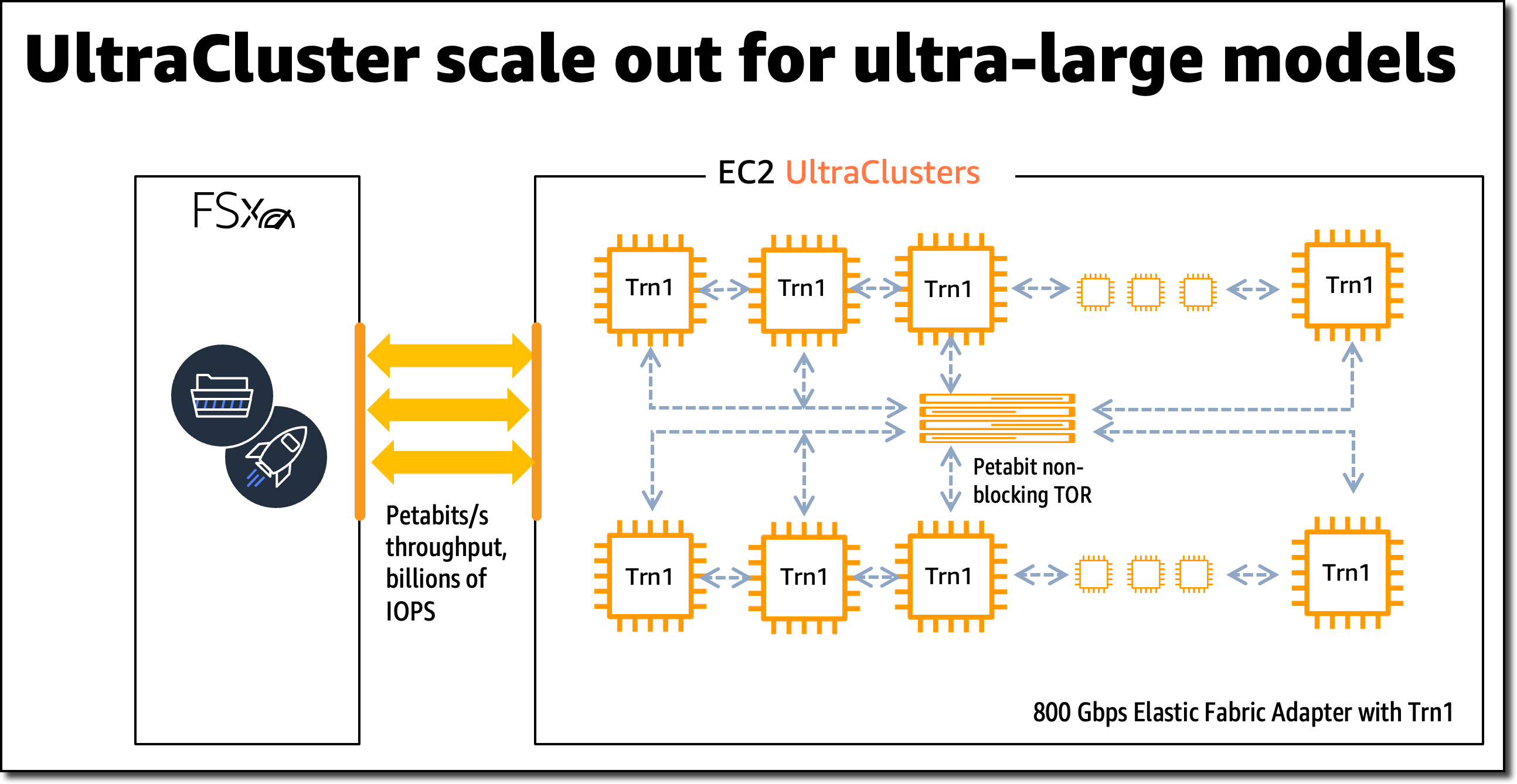
- Machine learning training is a complex problem requiring significant compute capacity and can benefit from specialized silicon. To hear more about the latest AWS designed silicon for deep learning training, attend “CMP313: Accelerate deep learning and innovate faster with AWS Trainium”. You will learn how Trainium delivers high performance and up to 50% savings in training costs over comparable GPU-based instances.
- Attend “CMP330: AWS managed services to run ML training workloads at scale with AWS Trainium” to hear about AWS managed services you can use to run your machine learning (ML) training workloads at scale on Trn1 instances.
- Attend “CMP209: AI parallelism explained: How Amazon Search scales deep-learning training” to learn more about Amazon Search trains large language models using various parallelism strategies and deploys them into production at scale.
- To learn about how to choose the right Amazon EC2 instance for ML training and inference, attend “CMP207: Choosing the right accelerator for training and inference”.
Cost Optimization
- Attend “CMP319: Optimize for cost and availability with capacity management” and learn how to use Amazon EC2 Capacity Reservations, On-Demand Capacity Reservations, and Savings Plans to lower costs so that you can focus on innovating.
- Do you want to host simple applications such phone systems, blogs, ecommerce sites etc. on the cloud? Amazon Lightsail is a cost-effective, easy-to-use cloud platform that’s ideal for simpler workloads and quick deployments. Attend “CMP218: Set your small business up for success with Amazon Lightsail” to learn how you can quickly deploy and configure virtually any application at a predictable monthly rate.
- Amazon EC2 Spot Instances are spare compute capacity available to you for less than On-Demand prices. To learn about the APIs and commands used to create Spot Instances, attend “CMP324: Spot the savings: Use Amazon EC2 Spot to optimize cloud deployments”.
Hear from our customers
We have several sessions this year where AWS customers are taking the stage to share their stories and details of exciting innovations made possible by AWS.
- Are you a machine learning (ML) startup trying to optimize your infrastructure costs? Attend “CMP226: How four customers reduced ML inference costs and drove innovation” to hear from Screening Eagle, Money Forward, Dataminr, and Actuate about how they have used Amazon EC2 Inf1 instances to get better performance at a lower cost per inference.
- Want to learn about the techniques Standard Chartered Bank uses to reduce waste and optimize cost and performance at scale? Attend “CMP213: Building a budget-conscious culture at Standard Chartered Bank” to learn how they’ve used a combination of AWS Savings Plan and Amazon EC2 spot instances to build critical large systems such as scaling applications, container platforms, and their grid for calculating risk and analytics.
- Come join us at “CMP208: Run large-scale graphics workloads with AWS, featuring Mircom and Snap” to learn about how Snap personalizes Bitmoji avatars and how Mircom creates digital twins of their fire alarm control panels and mission-critical smart building technologies. Learn how they leverage GPU-based instances in Amazon EC2 to unlock scalable graphics applications.
- To hear about metaverse experiences, from a panel including Epic Games, Surreal Events, and Cavrnus Inc., attend “CMP212: Metaverse experiences come to life with Amazon EC2 accelerated computing”.
Get started with hands-on sessions
Nothing like a hands-on session where you can learn by doing and get started easily with AWS compute. Our speakers and workshop assistants will help you every step of the way. Just bring your laptop to get started!
- Are you a developer or IT practitioner running Linux-based workloads in Amazon EC2 and looking for better price performance? Attend “CMP303: Get hands-on with AWS Graviton-based EC2 instances” to learn how to move a workload to AWS-Graviton based instances including containerized applications.
- Hugging Face has democratized the use of BERT-based natural language processing (NLP) models, which are a common foundation for many NLP applications. Attend “CMP206: Train & deploy a Hugging Face NLP model with AWS Trainium & AWS Inferentia” to learn how to use AWS ML silicon to train and run these popular models.
- Would you like to gain a solid skills foundation to run common HPC workloads using cloud technologies? Join us at “CMP305: Best practices for high performance computing in the cloud” to get hands-on experience setting up your own cluster in the cloud and running a sample application.
You’ll get to meet the global cloud community at AWS re:Invent and get an opportunity to learn, get inspired, and rethink what’s possible. So build your schedule in the re:Invent portal and get ready to hit the ground running. We invite you to stop by the AWS Compute booth and chat with our experts. We look forward to seeing you in Las Vegas!