Well, it’s been another historic year! We’ve watched in awe as the use of real-world generative AI has changed the tech landscape, and while we at the Architecture Blog happily participated, we also made every effort to stay true to our channel’s original scope, and your readership this last year has proven that decision was the right one.
AI/ML carries itself in the top posts this year, but we’re also happy to see that foundational topics like resiliency and cost optimization are still of great interest to our audience.
(By the way, if you were hoping for more AI/ML content, head on over to our sister channel, the AWS Machine Learning Blog!).
Without further ado, here are our top posts from 2024!
In keeping with Let’s Architect! series, we have our first of three favorites for the year. This set of resources helps you apply Well-Architected standards in practice.
As I said, Let’s Architect! has a winning series, and they’ve got a finger on the pulse of the tech world. This post about machine learning showcases some of the most exciting things happening at AWS.
Figure 3. Let’s Architect
If you’re more interested in generative AI, you can also take a look at another post from 2024: Let’s Architect! GenAI
Preparedness is another common theme in this year’s favorites. Michael, John, and Saurabh are well-versed in multi-Region architecture, and they’re here to share some strategies to contain failure impact.
Figure 4. When the application experiences an impairment using S3 resources in the primary Region, it fails over to use an S3 bucket in the secondary Region.
Let’s talk cost optimization. This post about a three-tier architecture that relies on the AWS Free Tier is a must-read for anyone looking for tips to help them avoid unnecessary costs (and that’s everyone).
Figure 5. Example of a three-tier architecture on AWS
As usual, Haleh & team are pros at making sure the Well-Architected Framework is current and relevant. Take a look at the enhanced and expanded guidance in all six pillars.
One more winning post from Luca, Federica, Vittorio, and Zamira! This collection of developer resources includes new ideas in AWS Lambda, Amazon Q Developer, and Amazon DynamoDB.
Frugality AND Well-Architected? What a winning combo! This post, inspired by the 2023 re:Invent keynote, outlines the seven laws of Frugal Architecture.
And finally, our number one post of the year! Amit and Luiz showcase a customer solution with real-world applications that builds on the guidelines of other posts in this list! Well done!
Figure 10. The Pilot Light scenario for a 3-tier application that has application servers and a database deployed in two Regions
Thank you!
As always, thanks to our contributors for their dedication and desire to share, and to you, our readers! We would be nothing with you. Literally.
For other top post lists, see our Top 10 and Top 5 posts from previous years.
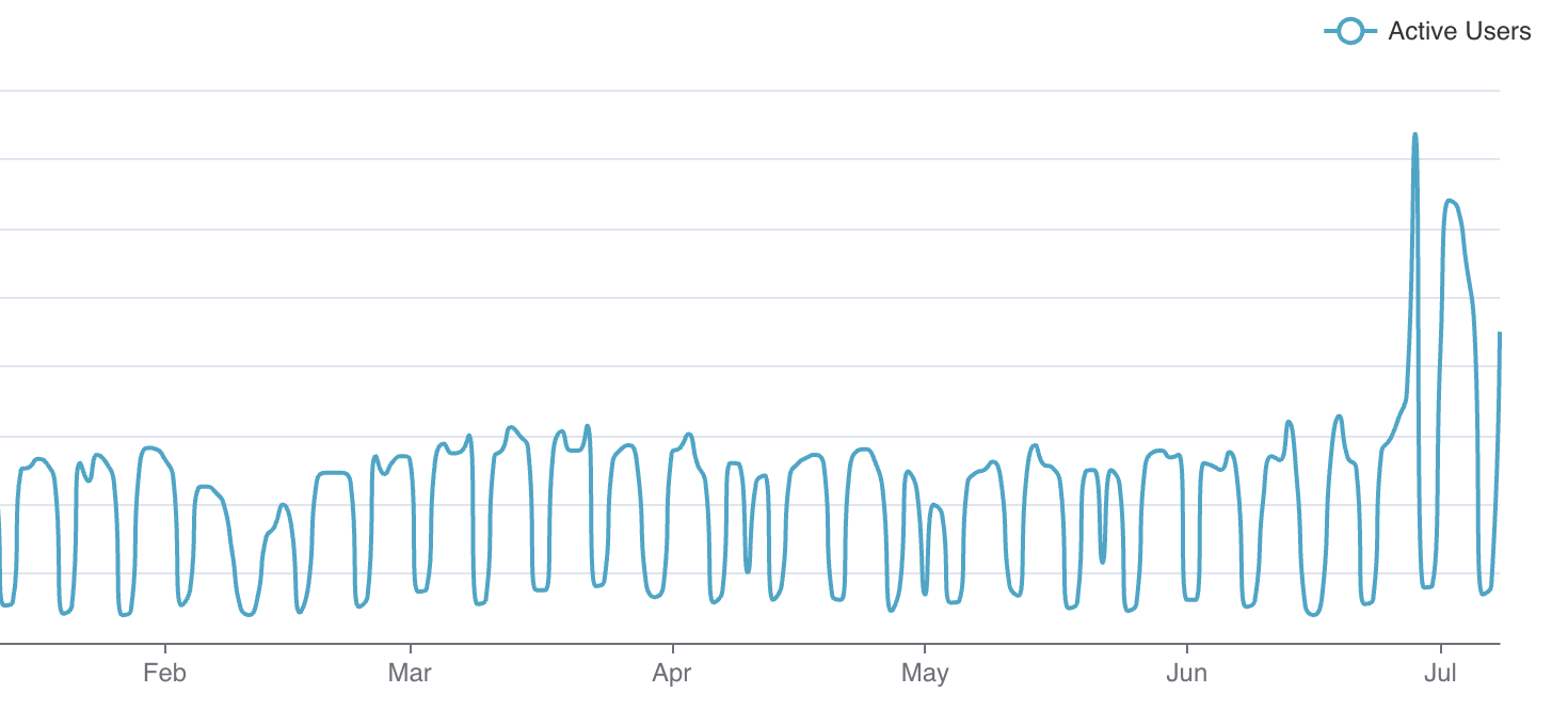
A month ago at QConSF, we showcased how Netflix utilizes Metaflow to power a diverse set of ML and AI use cases, managing thousands of unique Metaflow flows. This followed a previous blog on the same topic. Many of these projects are under constant development by dedicated teams with their own business goals and development best practices, such as the system that supports our content decision makers, or the system that ranks which language subtitles are most valuable for a specific piece of content.
As a central ML and AI platform team, our role is to empower our partner teams with tools that maximize their productivity and effectiveness, while adapting to their specific needs (not the other way around). This has been a guiding design principle with Metaflow since its inception.
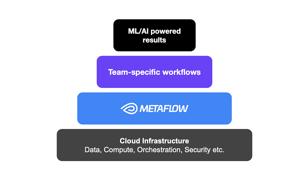
Metaflow infrastructure stack
Standing on the shoulders of our extensive cloud infrastructure, Metaflow facilitates easy access to data, compute, and production-grade workflow orchestration, as well as built-in best practices for common concerns such as collaboration, versioning, dependency management, and observability, which teams use to setup ML/AI experiments and systems that work for them. As a result, Metaflow users at Netflix have been able to run millions of experiments over the past few years without wasting time on low-level concerns.
A long standing FAQ: configurable flows
While Metaflow aims to be un-opinionated about some of the upper levels of the stack, some teams within Netflix have developed their own opinionated tooling. As part of Metaflow’s adaptation to their specific needs, we constantly try to understand what has been developed and, more importantly, what gaps these solutions are filling.
In some cases, we determine that the gap being addressed is very team specific, or too opinionated at too high a level in the stack, and we therefore decide to not develop it within Metaflow. In other cases, however, we realize that we can develop an underlying construct that aids in filling that gap. Note that even in that case, we do not always aim to completely fill the gap and instead focus on extracting a more general lower level concept that can be leveraged by that particular user but also by others. One such recurring pattern we noticed at Netflix is the need to deploy sets of closely related flows, often as part of a larger pipeline involving table creations, ETLs, and deployment jobs. Frequently, practitioners want to experiment with variants of these flows, testing new data, new parameterizations, or new algorithms, while keeping the overall structure of the flow or flows intact.
A natural solution is to make flows configurable using configuration files, so variants can be defined without changing the code. Thus far, there hasn’t been a built-in solution for configuring flows, so teams have built their bespoke solutions leveraging Metaflow’s JSON-typed Parameters, IncludeFile, and deploy-time Parameters or deploying their own home-grown solution (often with great pain). However, none of these solutions make it easy to configure all aspects of the flow’s behavior, decorators in particular.
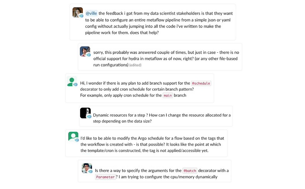
Requests for a feature like Metaflow Config
Outside Netflix, we have seen similar frequently asked questions on the Metaflow community Slack as shown in the user quotes above:
how can I adjust the @resource requirements, such as CPU or memory, without having to hardcode the values in my flows?
how to adjust the triggering @schedule programmatically, so our production and staging deployments can run at different cadences?
New in Metaflow: Configs!
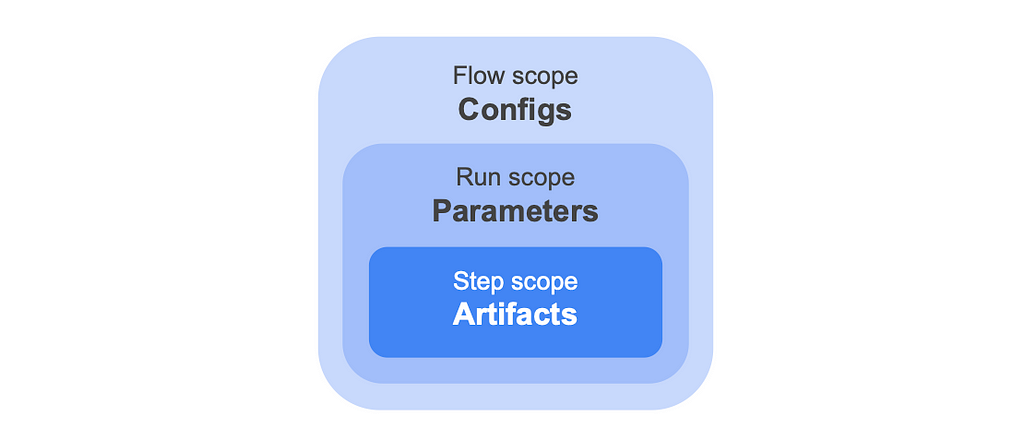
Today, to answer the FAQ, we introduce a new — small but mighty — feature in Metaflow: a Config object. Configs complement the existing Metaflow constructs of artifacts and Parameters, by allowing you to configure all aspects of the flow, decorators in particular, prior to any run starting. At the end of the day, artifacts, Parameters and Configs are all stored as artifacts by Metaflow but they differ in when they are persisted as shown in the diagram below:
Different data artifacts in Metaflow
Said another way:
An artifact is resolved and persisted to the datastore at the end of each task.
A parameter is resolved and persisted at the start of a run; it can therefore be modified up to that point. One common use case is to use triggers to pass values to a run right before executing. Parameters can only be used within your step code.
A config is resolved and persisted when the flow is deployed. When using a scheduler such as Argo Workflows, deployment happens when create’ing the flow. In the case of a local run, “deployment” happens just prior to the execution of the run — think of “deployment” as gathering all that is needed to run the flow. Unlike parameters, configs can be used more widely in your flow code, particularly, they can be used in step or flow level decorators as well as to set defaults for parameters. Configs can of course also be used within your flow.
As an example, you can specify a Config that reads a pleasantly human-readable configuration file, formatted as TOML. The Config specifies a triggering ‘@schedule’ and ‘@resource’ requirements, as well as application-specific parameters for this specific deployment:
[schedule]
cron = "0 * * * *"

[model]
optimizer = "adam"
learning_rate = 0.5

[resources]
cpu = 1
Using the newly released Metaflow 2.13, you can configure a flow with a Config like above, as demonstrated by this flow:
There is a lot going on in the code above, a few highlights:
you can refer to configs before they have been defined using ‘config_expr’.
you can define arbitrary parsers — using a string means the parser doesn’t even have to be present remotely!
From the developer’s point of view, Configs behave like dictionary-like artifacts. For convenience, they support the dot-syntax (when possible) for accessing keys, making it easy to access values in a nested configuration. You can also unpack the whole Config (or a subtree of it) with Python’s standard dictionary unpacking syntax, ‘**config’. The standard dictionary subscript notation is also available.
Since Configs turn into dictionary artifacts, they get versioned and persisted automatically as artifacts. You can access Configs of any past runs easily through the Client API. As a result, your data, models, code, Parameters, Configs, and execution environments are all stored as a consistent bundle — neatly organized in Metaflow namespaces — paving the way for easily reproducible, consistent, low-boilerplate, and now easily configurable experiments and robust production deployments.
More than a humble config file
While you can get far by accompanying your flow with a simple config file (stored in your favorite format, thanks to user-definable parsers), Configs unlock a number of advanced use cases. Consider these examples from the updated documentation:
You are not limited to using a single file: you can leverage a configuration manager like OmegaConf or Hydra to manage a hierarchy of cascading configuration files. You can also use a domain-specific tool for generating Configs, such as Netflix’s Metaboost which we cover below.
You can also generate configurations on the fly, e.g. fetch Configs from an external service, or inspect the execution environment, such as the current GIT branch, and include it as an extra piece of context in runs.
A major benefit of Config over previous more hacky solutions for configuring flows is that they work seamlessly with other features of Metaflow: you can run steps remotely and deploy flows to production, even when relying on custom parsers, without having to worry about packaging Configs or parsers manually or keeping Configs consistent across tasks. Configs also work with the Runner and Deployer.
The Hollywood principle: don’t call us, we’ll call you
When used in conjunction with a configuration manager like Hydra, Configs enable a pattern that is highly relevant for ML and AI use cases: orchestrating experiments over multiple configurations or sweeping over parameter spaces. While Metaflow has always supported sweeping over parameter grids easily using foreaches, it hasn’t been easily possible to alter the flow itself, e.g. to change @resources or @pypi/@conda dependencies for every experiment.
In a typical case, you trigger a Metaflow flow that consumes a configuration file, changing how a run behaves. With Hydra, you can invert the control: it is Hydra that decides what gets run based on a configuration file. Thanks to Metaflow’s new Runner and Deployer APIs, you can create a Hydra app that operates Metaflow programmatically — for instance, to deploy and execute hundreds of variants of a flow in a large-scale experiment.
Take a look at two interesting examples of this pattern in the documentation. As a teaser, this video shows Hydra orchestrating deployment of tens of Metaflow flows, each of which benchmarks PyTorch using a varying number of CPU cores and tensor sizes, updating a visualization of the results in real-time as the experiment progresses:
Metaboosting Metaflow — based on a true story
To give a motivating example of what configurations look like at Netflix in practice, let’s consider Metaboost, an internal Netflix CLI tool that helps ML practitioners manage, develop and execute their cross-platform projects, somewhat similar to the open-source Hydra discussed above but with specific integrations to the Netflix ecosystem. Metaboost is an example of an opinionated framework developed by a team already using Metaflow. In fact, a part of the inspiration for introducing Configs in Metaflow came from this very use case.
Metaboost serves as a single interface to three different internal platforms at Netflix that manage ETL/Workflows (Maestro), Machine Learning Pipelines (Metaflow) and Data Warehouse Tables (Kragle). In this context, having a single configuration system to manage a ML project holistically gives users increased project coherence and decreased project risk.
Configuration in Metaboost
Ease of configuration and templatizing are core values of Metaboost. Templatizing in Metaboost is achieved through the concept of bindings, wherein we can bind a Metaflow pipeline to an arbitrary label, and then create a corresponding bespoke configuration for that label. The binding-connected configuration is then merged into a global set of configurations containing such information as GIT repository, branch, etc. Binding a Metaflow, will also signal to Metaboost that it should instantiate the Metaflow flow once per binding into our orchestration cluster.
Imagine a ML practitioner on the Netflix Content ML team, sourcing features from hundreds of columns in our data warehouse, and creating a multitude of models against a growing suite of metrics. When a brand new content metric comes along, with Metaboost, the first version of the metric’s predictive model can easily be created by simply swapping the target column against which the model is trained.
Subsequent versions of the model will result from experimenting with hyper parameters, tweaking feature engineering, or conducting feature diets. Metaboost’s bindings, and their integration with Metaflow Configs, can be leveraged to scale the number of experiments as fast as a scientist can create experiment based configurations.
Scaling experiments with Metaboost bindings — backed by Metaflow Config
Consider a Metaboost ML project named `demo` that creates and loads data to custom tables (ETL managed by Maestro), and then trains a simple model on this data (ML Pipeline managed by Metaflow). The project structure of this repository might look like the following:
Metaboost will merge each experiment configuration (*.EXP*.yaml) into the global configuration (settings.configuration.yaml) individually at Metaboost command initialization. Let’s take a look at how Metaboost combines these configurations with a Metaboost command:
(venv-demo) ~/projects/metaboost-demo [branch=demoX]
$ metaboost metaflow settings show --yaml-path=configuration

binding=EXP_01:
model:                     -> defined in setting.configuration.yaml (global)
  fit_intercept: true
conda:                     -> defined in setting.configuration.yaml (global)
  numpy: 1.22.4
  "scikit-learn": 1.4.0
target_column: metricA     -> defined in setting.configuration.EXP_01.yaml
features:                  -> defined in setting.configuration.EXP_01.yaml
- runtime
- content_type
- top_billed_talent

binding=EXP_02:
model:                     -> defined in setting.configuration.yaml (global)
  fit_intercept: true
conda:                     -> defined in setting.configuration.yaml (global)
  numpy: 1.22.4
  "scikit-learn": 1.4.0
target_column: metricA     -> defined in setting.configuration.EXP_02.yaml
features:                  -> defined in setting.configuration.EXP_02.yaml
- runtime
- director
- box_office
Metaboost understands it should deploy/run two independent instances of training.py — one for the EXP_01 binding and one for the EXP_02 binding. You can also see that Metaboost is aware that the tables and ETL workflows are not bound, and should only be deployed once. These details of which artifacts to bind and which to leave unbound are encoded in the project’s top-level metaboost.yaml file.
(venv-demo) ~/projects/metaboost-demo [branch=demoX] $ metaboost project list
Below is a simple Metaflow pipeline that fetches data, executes feature engineering, and trains a LinearRegression model. The work to integrate Metaboost Settings into a user’s Metaflow pipeline (implemented using Metaflow Configs) is as easy as adding a single mix-in to the FlowSpec definition:
from metaflow import FlowSpec, Parameter, conda_base, step from custom.data import feature_engineer, get_data from metaflow.metaboost import MetaboostSettings
@step def start(self): # get show_settings() for free with the mixin # and get convenient debugging info self.show_settings(exclude_patterns=["artifact*", "system*"])
self.next(self.get_features)
@step def get_features(self): # feature engineers on our extracted data self.fe_df = feature_engineer( # loads data from our ETL pipeline data=get_data(prediction_date=self.prediction_date), features=self.settings.configuration.features + [self.settings.configuration.target_column] )
self.next(self.train)
@step def train(self): from sklearn.linear_model import LinearRegression
The Metaflow Config is added to the FlowSpec by mixing in the MetaboostSettings class. Referencing a configuration value is as easy as using the dot syntax to drill into whichever parameter you’d like.
Finally let’s take a look at the output from our sample Metaflow above. We execute experiment EXP_01 with
metaboost metaflow run --binding=EXP_01
which upon execution will merge the configurations into a single settings file (shown previously) and serialize it as a yaml file to the .metaboost/settings/compiled/ directory.
You can see the actual command and args that were sub-processed in the Metaboost Execution section below. Please note the –config argument pointing to the serialized yaml file, and then subsequently accessible via self.settings. Also note the convenient printing of configuration values to stdout during the start step using a mixed in function named show_settings().
(venv-demo) ~/projects/metaboost-demo [branch=demoX] $ metaboost metaflow run --binding=EXP_01
Metaflow 2.12.39+nflxfastdata(2.13.5);nflx(2.13.5);metaboost(0.0.27) executing DemoTraining for user:dcasler Validating your flow... The graph looks good! Bootstrapping Conda environment... (this could take a few minutes) All packages already cached in s3. All environments already cached in s3.
Workflow starting (run-id 50), see it in the UI at https://metaflowui.prod.netflix.net/DemoTraining/50
[50/get_features/251640840] Task is starting. [50/get_features/251640840] Task finished successfully.
[50/train/251640854] Task is starting. [50/train/251640854] Fit slope: 0.4702672504331096 [50/train/251640854] Fit intercept: -6.247919678070083 [50/train/251640854] Task finished successfully.
[50/end/251640868] Task is starting. [50/end/251640868] Task finished successfully.
Done! See the run in the UI at https://metaflowui.prod.netflix.net/DemoTraining/50
Takeaways
Metaboost is an integration tool that aims to ease the project development, management and execution burden of ML projects at Netflix. It employs a configuration system that combines git based parameters, global configurations and arbitrarily bound configuration files for use during execution against internal Netflix platforms.
Integrating this configuration system with the new Config in Metaflow is incredibly simple (by design), only requiring users to add a mix-in class to their FlowSpec — similar to this example in Metaflow documentation — and then reference the configuration values in steps or decorators. The example above templatizes a training Metaflow for the sake of experimentation, but users could just as easily use bindings/configs to templatize their flows across target metrics, business initiatives or any other arbitrary lines of work.
Try it at home
It couldn’t be easier to get started with Configs! Just
If you have any questions or feedback about Config (or other Metaflow features), you can reach out to us at the Metaflow community Slack.
Acknowledgments
We would like to thank Outerbounds for their collaboration on this feature; for rigorously testing it and developing a repository of examples to showcase some of the possibilities offered by this feature.
AI, machine learning (ML), and data science infuse our daily lives, from the recommendation functionality on music apps to technologies that influence our healthcare, transport, education, defence, and more.
What jobs will be affected by AL, ML, and data science remains to be seen, but it is increasingly clear that students will need to learn something about these topics. There will be new concepts to be taught, new instructional approaches and assessment techniques to be used, new learning activities to be delivered, and we must not neglect the professional development required to help educators master all of this.
As AI and data science are incorporated into school curricula and teaching and learning materials worldwide, we ask: What’s the research basis for these curricula, pedagogy, and resource choices?
In 2024, we showcased researchers who are investigating how AI can be leveraged to support the teaching and learning of programming. But in 2025, we look at what should be taught about AI, ML, and data science in schools and how we should teach this.
Our 2025 seminar speakers — so far!
We are very excited that we have already secured several key researchers in the field.
On 21 January, Shuchi Grover will kick off the seminar series by giving an important overview of AI in the K–12 landscape, including developing both AI literacy and AI ethics. Shuchi will provide concrete examples and recently developed frameworks to give educators practical insights on the topic.
Our second session will focus on a teacher professional development (PD) programme to support the introduction of AI in Upper Bavarian schools. Franz Jetzinger from the Technical University of Munich will summarise the PD programme and share how teachers implemented the topic in their classroom, including the difficulties they encountered.
Again from Germany, Lukas Höper from Paderborn University, with Carsten Schulte will describe important research on data awareness and introduce a framework that is likely to be key for learning about data-driven technology. The pair will talk about the Data Awareness Framework and how it has been used to help learners explore, evaluate, and be empowered in looking at the role of data in everyday applications.
Our April seminar will see David Weintrop from the University of Maryland introduce, with his colleagues, a data science curriculum called API Can Code, aimed at high-school students. The group will highlight the strategies needed for integrating data science learning within students’ lived experiences and fostering authentic engagement.
Later in the year, Jesús Moreno-Leon from the University of Seville will help us consider the thorny but essential question of how we measure AI literacy. Jesús will present an assessment instrument that has been successfully implemented in several research studies involving thousands of primary and secondary education students across Spain, discussing both its strengths and limitations.
What to expect from the seminars
Our seminars are designed to be accessible to anyone interested in the latest research about AI education — whether you’re a teacher, educator, researcher, or simply curious. Each session begins with a presentation from our guest speaker about their latest research findings. We then move into small groups for a short discussion and exchange of ideas before coming back together for a Q&A session with the presenter.
Attendees of our 2024 series told us that they valued that the talks “explore a relevant topic in an informative way“, the “enthusiasm and inspiration”, and particularly the small-group discussions because they “are always filled with interesting and varied ideas and help to spark my own thoughts”.
The seminars usually take place on Zoom on the first Tuesday of each month at 17:00–18:30 GMT / 12:00–13:30 ET / 9:00–10:30 PT / 18:00–19:30 CET.
You can find out more about each seminar and the speakers on our upcoming seminar page. And if you are unable to attend one of our talks, you can watch them from our previous seminar page, where you will also find an archive of all of our previous seminars dating back to 2020.
How to sign up
To attend the seminars, please register here. You will receive an email with the link to join our next Zoom call. Once signed up, you will automatically be notified of upcoming seminars. You can unsubscribe from our seminar notifications at any time.
The company’s Mobile Threat Hunting feature uses a combination of malware signature-based detection, heuristics, and machine learning to look for anomalies in iOS and Android device activity or telltale signs of spyware infection. For paying iVerify customers, the tool regularly checks devices for potential compromise. But the company also offers a free version of the feature for anyone who downloads the iVerify Basics app for $1. These users can walk through steps to generate and send a special diagnostic utility file to iVerify and receive analysis within hours. Free users can use the tool once a month. iVerify’s infrastructure is built to be privacy-preserving, but to run the Mobile Threat Hunting feature, users must enter an email address so the company has a way to contact them if a scan turns up spyware—as it did in the seven recent Pegasus discoveries.
Around the world, organizations are evaluating and embracing artificial intelligence (AI) and machine learning (ML) to drive innovation and efficiency. From accelerating research and enhancing customer experiences to optimizing business processes, improving patient outcomes, and enriching public services, the transformative potential of AI is being realized across sectors. Although using emerging technologies helps drive positive outcomes, leaders worldwide must balance these benefits with the need to maintain security, compliance, and resilience. Many organizations, including those in the public sector and regulated industries, are investing in generative AI applications powered by large language models (LLMs) and other foundation models (FMs) because these applications can transform and scale their work and provide better experiences for customers. Beyond computing power, unlocking this AI potential resides in the AI applications that organizations can create based on a variety of AI/ML development services, models, and data sources. Organizations must navigate the complexity of building AI applications in light of existing and emerging regulatory regimes while verifying that their AI applications and related data are secure, protected, and resilient to risks and threats.
AWS offers a wide range of AI/ML services and capabilities, built on our sovereign-by-design foundation, that are making it simpler for our customers to meet their digital sovereignty needs while getting the security, control, compliance, and resilience that they need. For example, Amazon Bedrock is a fully managed service that offers a choice of high-performing FMs from leading AI companies such as AI21 Labs, Anthropic, Cohere, Meta, Mistral AI, and Stability AI through a single API, along with a broad set of capabilities to build generative AI applications with security, privacy, and responsible AI. Amazon SageMaker provides tools and infrastructure to build, train, and deploy ML models at scale while supporting responsible AI with governance controls and access to pretrained models.
Innovating securely across the AI lifecycle
Security is and always has been our top priority at AWS. AWS customers benefit from our ongoing investment in data centers, networks, custom hardware, and secure software services, built to satisfy the requirements of the most security-sensitive organizations, including the government, healthcare, and financial services. We have always believed that it is essential that customers have control over their data and its location. That’s why we architected the AWS Cloud to be secure and sovereign-by-design from day one. We remain committed to giving our customers more control and choice so that they can use the full power of AWS while meeting their unique digital sovereignty needs.
As organizations develop and implement generative AI, they want to make sure that their data and applications are secured across the AI lifecycle, including data preparation, training, and inferencing. To help ensure the confidentiality and integrity of customer data, all of our Nitro-based Amazon Elastic Compute Cloud (Amazon EC2) instances that run ML accelerators such as AWS Inferentia and AWS Trainium, and graphics processing units (GPUs) such as P4, P5, G5, and G6, are backed by the industry-leading security capabilities of the AWS Nitro System. By design, there is no mechanism for anyone at AWS to access Nitro EC2 instances that customers use to run their workloads. The NCC Group, an independent cybersecurity firm, has validated the design of the Nitro System.
We take a secure approach to generative AI and make it practical for our customers to secure their generative AI workloads across the generative AI stack so that they can focus on building and scaling. All AWS services—including generative AI services—support encryption, and we continue to innovate and invest in controls and encryption features that allow our customers to encrypt everything everywhere.
For example, Amazon Bedrock uses encryption to protect data in transit and at rest, and data remains in the AWS Region where Amazon Bedrock is being used. Customer data, such as prompts, completions, custom models, and data used for fine-tuning or continued pre-training, is not used for Amazon Bedrock service improvement and is never shared with third-party model providers. When customers fine-tune a model in Amazon Bedrock, the data is never exposed to the public internet, never leaves the AWS network, is securely transferred through a customer’s virtual private cloud (VPN), and is encrypted in transit and at rest.
SageMaker protects ML model artifacts and other system artifacts by encrypting data in transit and at rest. Amazon Bedrock and SageMaker integrate with AWS Key Management Service (AWS KMS) so that customers can securely manage cryptographic keys. AWS KMS is designed so that no one—not even AWS employees—can retrieve plaintext keys from the service.
Developing responsibly
The responsible development and use of AI is a priority for AWS. We believe that AI should take a people-centric approach that makes AI safe, fair, secure, and robust. We are committed to supporting customers with responsible AI and helping them build fairer and more transparent AI applications to foster trust, meet regulatory requirements, and use AI to benefit their business and stakeholders. AWS is the first major cloud service provider to announce ISO/IEC 42001 accredited certification for AI services, covering Amazon Bedrock, Amazon Q Business, Amazon Textract, and Amazon Transcribe. ISO/IEC 42001 is an international management system standard that outlines requirements and controls for organizations to promote the responsible development and use of AI systems.
We take responsible AI from theory into practice by providing the necessary tools, guidance, and resources, including Amazon Bedrock Guardrails to help implement safeguards tailored to customer generative AI applications and aligned with their responsible AI policies, or Model Evaluation on Amazon Bedrock to evaluate, compare, and select the best FMs for specific use cases based on custom metrics, such as accuracy, robustness, and toxicity. Additionally, Amazon SageMaker Model Monitor automatically detects and alerts customers of inaccurate predictions from deployed models. We continue to publish AI Service Cards to enhance transparency by providing a single place to find information on the intended use cases and limitations, responsible AI design choices, and performance optimization best practices for our AI services and models.
Building resilience
Resilience plays a pivotal role in the development of any workload, and AI/ML workloads are no different. Customers need to know that their workloads in the cloud will continue to operate in the face of natural disasters, network disruptions, or disruptions due to geopolitical crises. AWS delivers the highest network availability of any cloud provider and is the only cloud provider to offer three or more Availability Zones (AZs) in all Regions, providing more redundancy. Understanding and prioritizing resilience is crucial for generative AI workloads to meet organizational availability and business continuity requirements. We have published guidance on designing generative AI workloads for resilience. To enable higher throughput and enhanced resilience during periods of peak demands in Amazon Bedrock, customers can use cross-region inference to distribute traffic across multiple Regions. For customers with specific European Union data sovereignty requirements, we are launching the AWS European Sovereign Cloud in 2025 to offer an additional layer of control and resilience.
Supporting choice and flexibility
It’s important that customers have access to diverse AI technologies, while having the freedom to choose the right solutions to meet their needs. AWS provides more diversity, choice, and flexibility so that customers can select the AI solution that best aligns with their specific requirements, whether that’s using open-source models, proprietary solutions, or their own custom AI models. For example, we understand the importance of open-source AI in fostering transparency, collaboration, and rapid innovation. Open-source models enable scrutiny of vulnerabilities, drive security improvements, and support research on AI safety. Amazon SageMaker JumpStart provides pretrained, open-source models for a wide range of common use cases. To provide practitioners and developers with the guidance and tools that they need to create secure-by-design AI systems, we are a founding member of the open-source initiative Coalition for Secure AI (CoSAI).
Also, our commitment to portability and interoperability helps ensure that customers can move easily between environments. For customers changing IT providers, we’ve taken concrete steps to lower costs, and AWS is actively engaged in efforts to facilitate switching between cloud providers, including through our support of the Cloud Infrastructure Service Providers in Europe (CISPE)Cloud Switching Framework, which lays out guidance to assist providers and customers in the switching process. This gives organizations the flexibility to adapt their cloud and AI strategies as their needs evolve.
We remain committed to providing customers with a choice of diverse AI technologies, along with secure and compliant ways to build their AI applications throughout the development lifecycle. Through this approach, customers can enhance the security, compliance, and resilience of their systems.
If you have feedback about this post, submit comments in the Comments section below. If you have questions about this post, contact AWS Support.
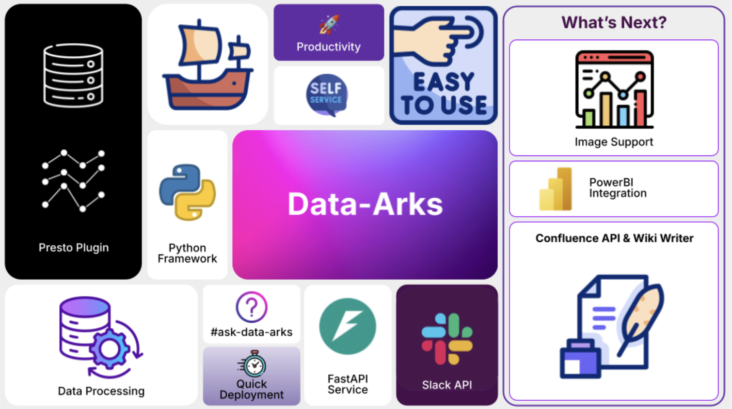
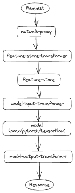
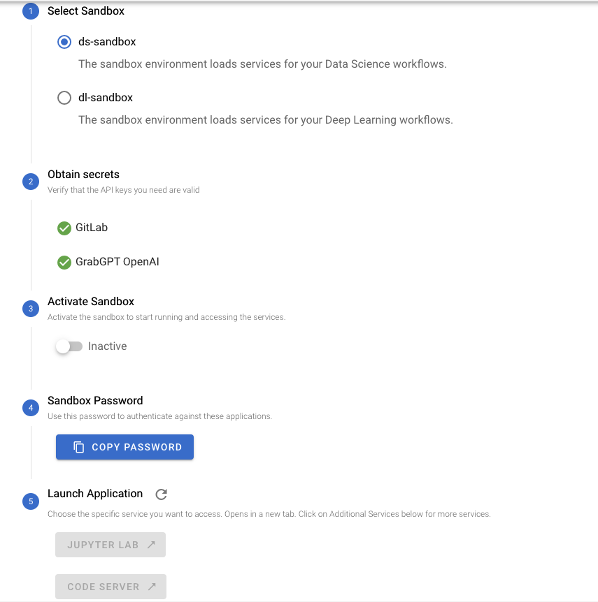
At Grab, we are committed to leveraging the power of technology to deliver the best services to our users and partners. As part of this commitment, we have developed the LLM-Kit, a comprehensive framework designed to supercharge the setup of production-ready Generative AI applications. This blog post will delve into the features of the LLM-Kit, the problems it solves, and the value it brings to our organisation.
Challenges
The introduction of the LLM-Kit has significantly addressed the challenges encountered in LLM application development. The involvement of sensitive data in AI applications necessitates that security remains a top priority, ensuring data safety is not compromised during AI application development.
Concerns such as scalability, integration, monitoring, and standardisation are common issues that any organisation will face in their LLM and AI development efforts.
The LLM-Kit has empowered Grab to pursue LLM application development and the rollout of Generative AI efficiently and effectively in the long term.
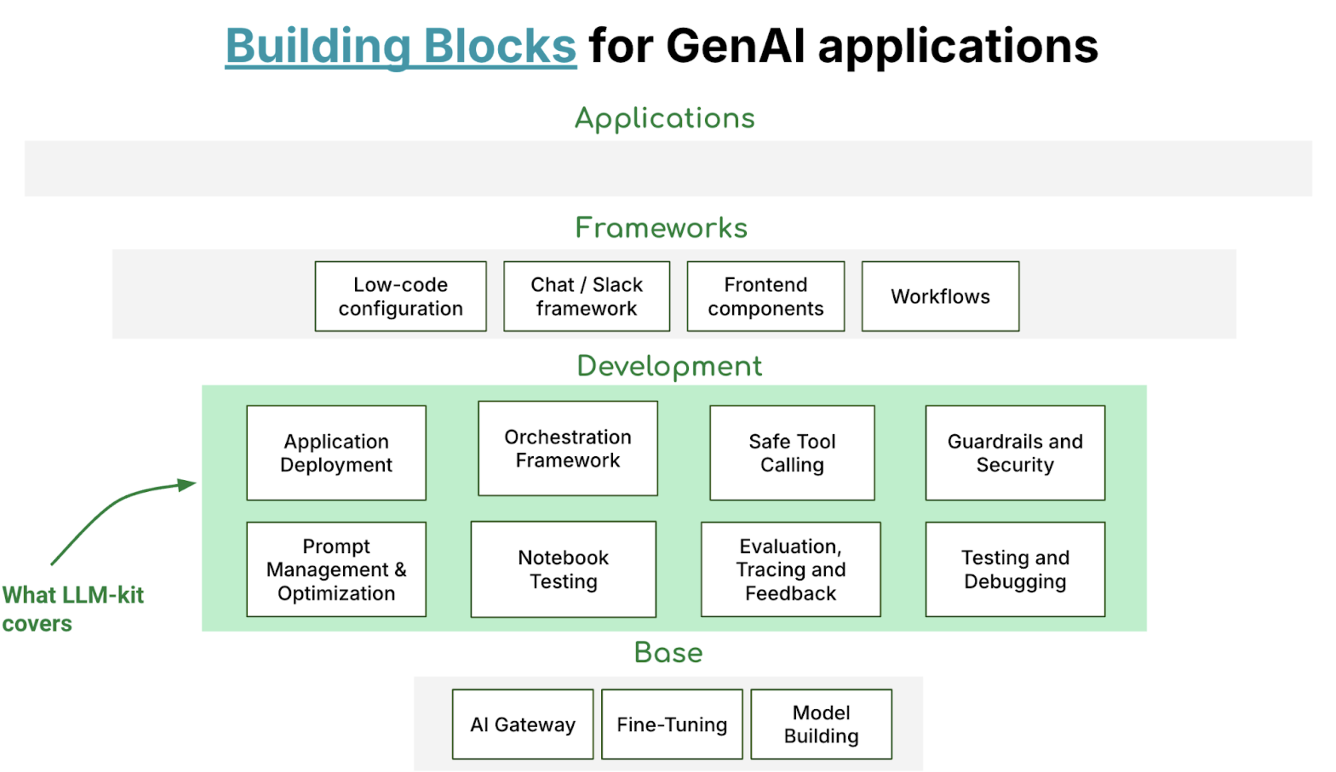
Introducing the LLM-Kit
The LLM-Kit is our solution to these challenges. Since the introduction of the LLM Kit, it has helped onboard hundreds of GenAI applications at Grab and has become the de facto choice for developers. It is a comprehensive framework designed to supercharge the setup of production-ready LLM applications. The LLM-Kit provides:
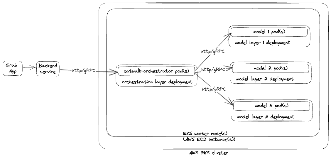
Pre-configured structure: The LLM-Kit comes with a pre-configured structure containing an API server, configuration management, a sample LLM Agent, and tests.
Integrated tech stack: The LLM-Kit integrates with Poetry, Gunicorn, FastAPI, LangChain, LangSmith, Hashicorp Vault, Amazon EKS, and Gitlab CI pipelines to provide a robust and end-to-end tech stack for LLM application development.
Observability: The LLM-Kit features built-in observability with Datadog integration and LangSmith, enabling real-time monitoring of LLM applications.
Config & secret management: The LLM-Kit utilises Python’s configparser and Vault for efficient configuration and secret management.
Authentication: The LLM-Kit provides built-in OpenID Connect (OIDC) auth helpers for authentication to Grab’s internal services.
API documentation: The LLM-Kit features comprehensive API documentation using Swagger and Redoc.
Redis & vector databases integration: The LLM-Kit integrates with Redis and Vector databases for efficient data storage and retrieval.
Deployment pipeline: The LLM-Kit provides a deployment pipeline for staging and production environments.
Evaluations: The LLM-Kit seamlessly integrates with LangSmith, utilising its robust evaluations framework to ensure the quality and performance of the LLM applications.
In addition to these features, the team has also included a cookbook with many commonly used examples within the organisation providing a valuable resource for developers. Our cookbook includes a diverse range of examples, such as persistent memory agents, Slackbot LLM agents, image analysers and full-stack chatbots with user interfaces, showcasing the versatility of the LLM-Kit.
The value of the LLM-Kit
The LLM-Kit brings significant value to our teams at Grab:
Increased development velocity: By providing a pre-configured structure and integrated tech stack, the LLM-Kit accelerates the development of LLM applications.
Improved observability: With built-in LangSmith and Datadog integration, teams can monitor their LLM applications in real-time, enabling faster issue detection and resolution.
Enhanced security: The LLM-Kit’s built-in OIDC auth helpers and secret management using Vault ensure the secure development and deployment of LLM applications.
Efficient data management: The integration with Vector databases facilitates efficient data storage and retrieval, crucial for the performance of LLM applications.
Standardisation: The LLM-Kit provides a paved-road framework for building LLM applications, promoting best practices and standardisation across teams.
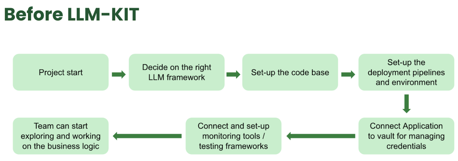
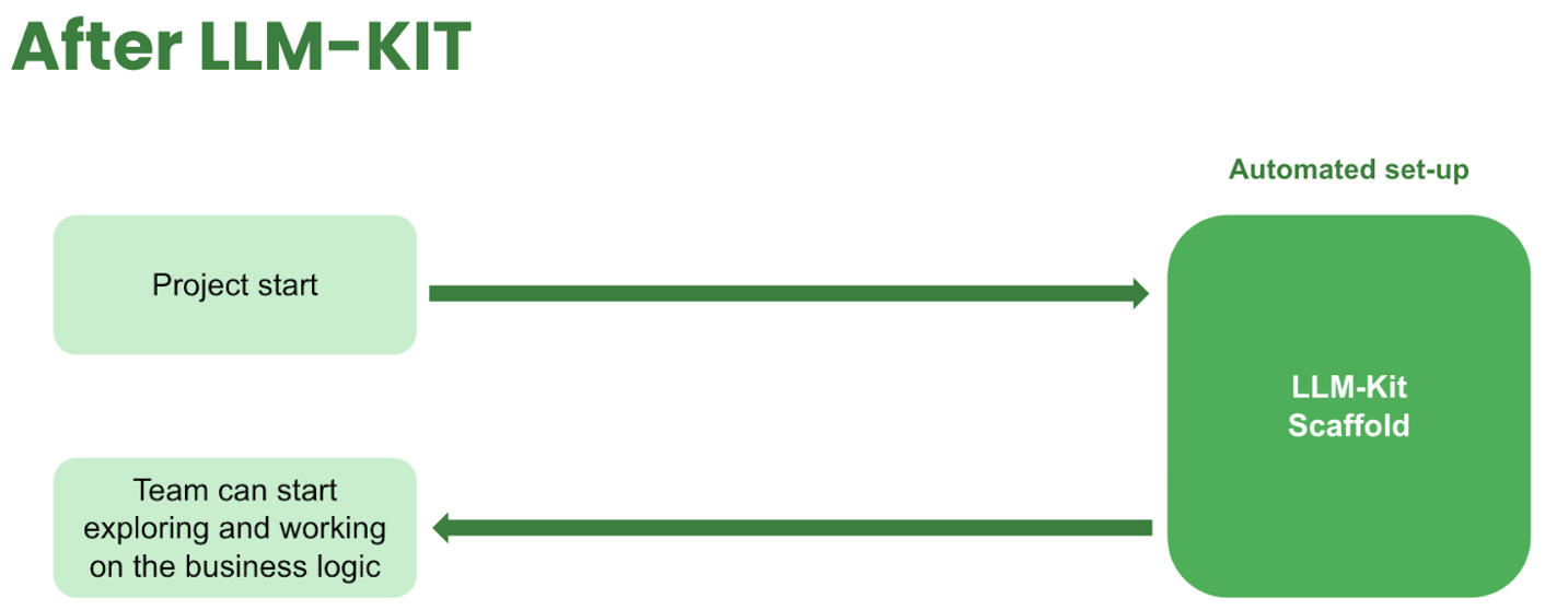
Through the LLM-Kit, we can save an estimate of 1.5 weeks before teams start working on their first feature.
Figure 1. Project development process before LLM-Kit
Figure 2. Project development process after LLM-Kit
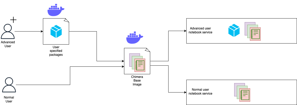
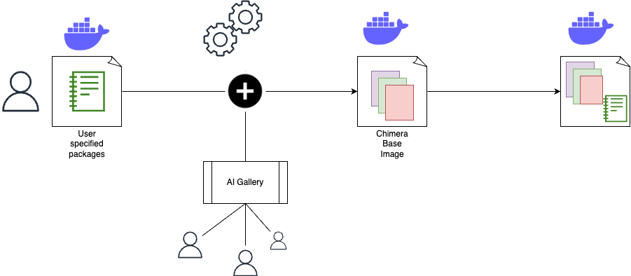
Architecture design and technical implementation
The LLM-Kit is designed with a modular architecture that promotes scalability, flexibility, and ease of use.
Figure 3. LLM-Kit modules
Automated steps
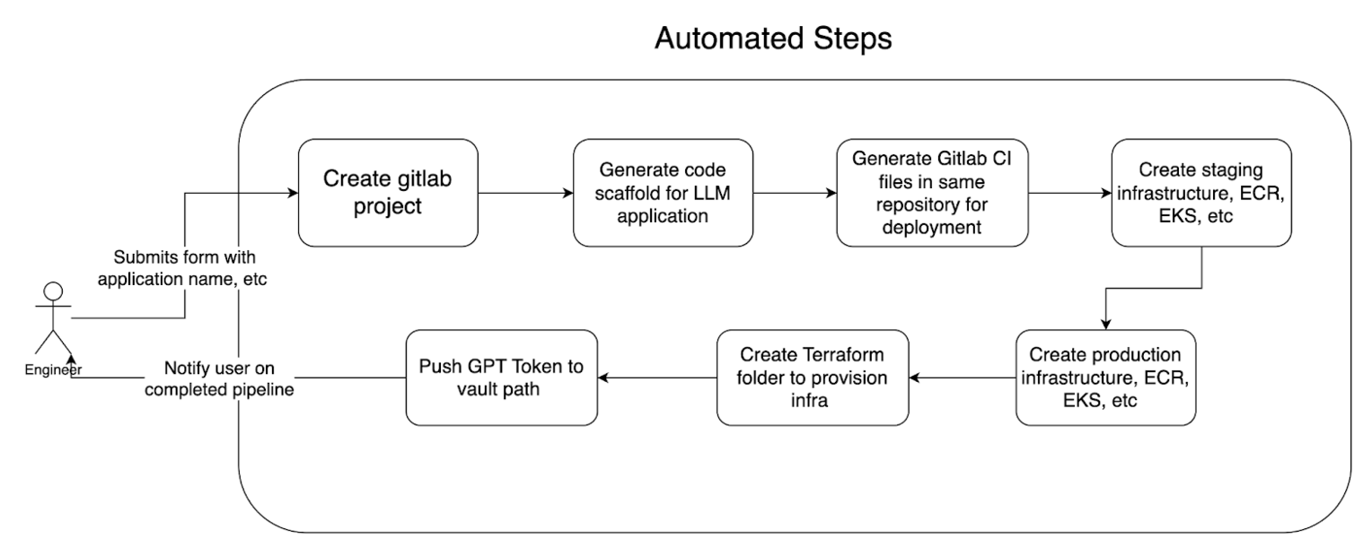
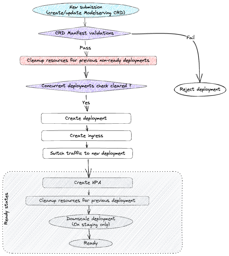
To better illustrate the technical implementation of the LLM-Kit, let’s take a look at figure 4 which outlines the step-by-step process of how an LLM application is generated with the LLM-Kit:
Figure 4. Process of generating LLM apps using LLM-Kit
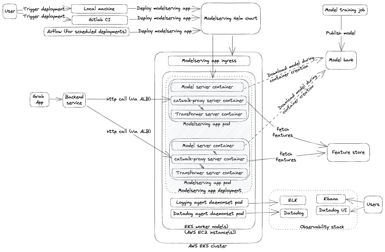
The process begins when an engineer submits a form with the application name and other relevant details. This triggers the creation of a GitLab project, followed by the generation of a code scaffold specifically designed for the LLM application. GitLab CI files are then generated within the same repository to handle continuous integration and deployment tasks. The process continues with the creation of staging infrastructure, including components like Elastic Container Registry (ECR) and Elastic Kubernetes Service (EKS). Additionally, a Terraform folder is created to provision the necessary infrastructure, eventually leading to the deployment of production infrastructure. At the end of the pipeline, a GPT token is pushed to a secure Vault path, and the engineer is notified upon the successful completion of the pipeline.
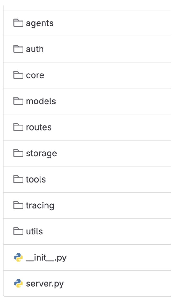
Scaffold code structure
The scaffolded code is broken down into multiple folders:
Agents: Contains the code to initialise an agent. We have gone ahead with LangChain as the agent framework; essentially the entry point for the endpoint defined in the Routes folder.
Auth: Authentication and authorisation module for executing some of the APIs within Grab.
Core: Includes extracting all configurations (i.e. GPT token) and secret decryption for running the LLM application.
Models: Used to define the structure for the core LLM APIs within Grab.
Routes: REST API endpoint definitions for the LLM Applications. It comes with health check, authentication, authorisation, and a simple agent by default.
Storage: Includes connectivity with PGVector, our managed vector database within Grab and database schemas.
Tools: Functions which are used as tools for the LLM Agent.
Tracing: Integration with our tracing and monitoring tools to monitor various metrics for a production application.
Utils: Default folder for utility functions.
Figure 5. Scaffold code structure
Infrastructure provisioning and deployment
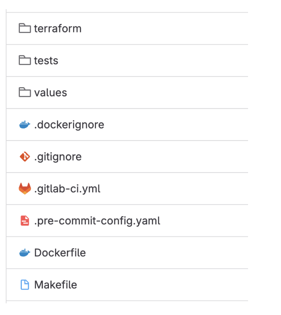
Within the same codebase, we have integrated a comprehensive pipeline that automatically scaffolds the necessary code for infrastructure provisioning, deployment, and build processes. Using Terraform, the pipeline provisions the required infrastructure seamlessly. The deployment pipelines are defined in the .gitlab-ci.yml file, ensuring smooth and automated deployments. Additionally, the build process is specified in the Dockerfile, allowing for consistent builds. This automated scaffolding streamlines the development workflow, enabling developers to focus on writing business logic without worrying about the underlying infrastructure and deployment complexities.
Figure 6. Pipeline infrastructure
RAG scaffolding
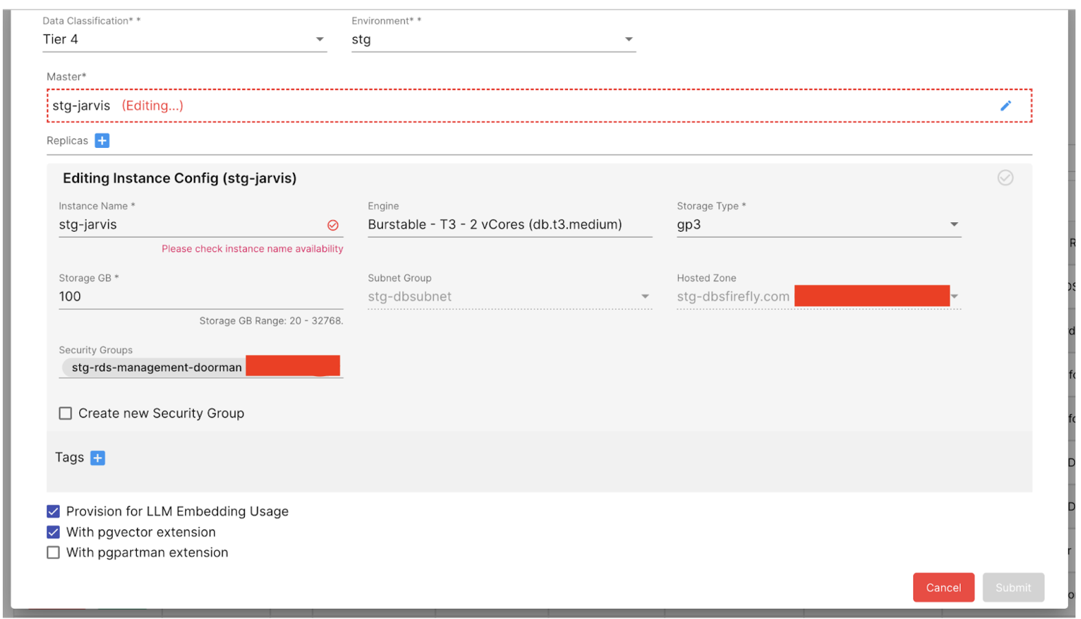
At Grab, we’ve established a streamlined process for setting up a vector database (PGVector) and whitelisting the service using the LLM-Kit. Once the form (figure 7) is submitted, you can access the credentials and database host path. The secrets will be automatically added to the Vault path. Engineers will then only need to include the DB host path in the configuration file of the scaffolded LLM-Kit application.
Figure 7. Form submitted to access credentials and database host path
Conclusion
The LLM-Kit is a testament to Grab’s commitment to fostering innovation and growth in AI and ML. By addressing the challenges faced by our teams and providing a comprehensive, scalable, and flexible framework for LLM application development, the LLM-Kit is paving the way for the next generation of AI applications at Grab.
Growth and future plans
Looking ahead, the LLM-Kit team aims to significantly enhance the web server’s concurrency and scalability while providing reliable and easy-to-use SDKs. The team plans to offer reusable and composable LLM SDKs, including evaluation and guardrails frameworks, to enable service owners to build feature-rich Generative AI programs with ease. Key initiatives also include the development of a CLI for version updates and dev tooling, as well as a polling-based agent serving function. These advancements are designed to drive innovation and efficiency within the organisation, ultimately providing a more seamless and efficient development experience for engineers.
We would like to acknowledge and thank Pak Zan Tan, Han Su, and Jonathan Ku from the Yoshi team and Chen Fei Lee from the MEKS team for their contribution to this project under the leadership of Padarn George Wilson.
Join us
Grab is the leading superapp platform in Southeast Asia, providing everyday services that matter to consumers. More than just a ride-hailing and food delivery app, Grab offers a wide range of on-demand services in the region, including mobility, food, package and grocery delivery services, mobile payments, and financial services across 700 cities in eight countries.
Powered by technology and driven by heart, our mission is to drive Southeast Asia forward by creating economic empowerment for everyone. If this mission speaks to you, join our team today!
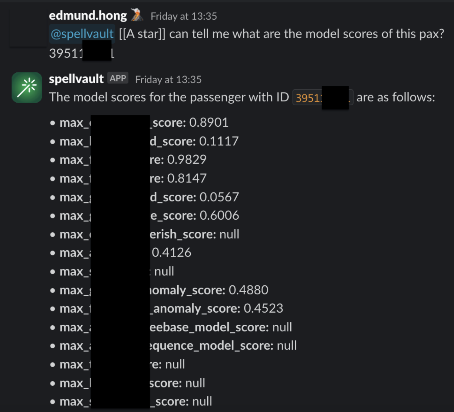
In the initial article, LLM Powered Data Classification, we addressed how we integrated Large Language Models (LLM) to automate governance-related metadata generation. The LLM integration enabled us to resolve challenges in Gemini, such as restrictions on the customisation of machine learning classifiers and limitations of resources to train a customised model. Gemini is a metadata generation service built internally to automate the tag generation process using a third-party data classification service. We also focused on LLM-powered column-level tag classifications. The classified tags, combined with Grab’s data privacy rules, allowed us to determine sensitivity tiers of data entities. The affordability of the model also enables us to scale it to cover more data entities in the company. The initial model scanned more than 20,000 data entries, at an average of 300-400 entities per day. Despite its remarkable performance, we were aware that there was room for improvement in the areas of data classification and prompt evaluation.
Improving the model post-rollout
Since its launch in early 2024, our model has gradually grown to cover the entire data lake. To date, the vast majority of our data lake tables have undergone analysis and classification by our model. This has significantly reduced the workload for Grabbers. Instead of manually classifying all new or existing tables, Grabbers can now rely on our model to assign the appropriate classification tier accurately.
Despite table classification being automated, the data pipeline still requires owners to manually perform verification to prevent any misclassifications. While it is impossible to entirely eliminate human oversight from critical machine learning workflows, the team has dedicated substantial time post-launch to refining the model, thereby safely minimising the need for human intervention.
Utilising post-rollout data
Following the deployment of our model and receipt of extensive feedback from table owners, we have accumulated a large dataset to further enhance the model. This data, coupled with the dataset of manual classifications from the Data Governance Office to ensure compliance with information classification protocols, serves as the training and testing datasets for the second iteration of our model.
Model improvements with prompt engineering
Expanding the evaluation and testing data allowed us to uncover weaknesses in the previous model. For instance, we discovered that seemingly innocuous table columns like “business email” could contain entries with Personal Identifiable Information (PII) data.
An example of this would be a business that uses a personal email address containing a legal name—a discrepancy that would be challenging for even human reviewers to detect. Additionally, we discovered nested JSON structures occasionally included personal names, phone numbers, and email addresses hidden among other non-PII metadata. Lastly, we identified passenger communications with Grab occasionally mentioning legal names, phone numbers, and other PII, despite most of the content being non-PII.
Ultimately, we hypothesised the model’s main issue was model capacity. The model displayed difficulty focusing on large data samples containing a mixture of PII and non-PII data despite having a good understanding of what constitutes PII. Just like humans, when given high volumes of tasks to work on simultaneously, the model’s effectiveness is reduced. In the original model, 13 out of 21 tags were aimed at distinguishing different types of non-PII data. This took up significant model capacity and distracted the model from its actual task: identifying PII data.
To prevent the model from being overwhelmed, large tasks are divided into smaller, more manageable tasks, allowing the model to dedicate more attention to each task. The following measures were taken to free up model capacity:
Splitting the model into two parts to make problem solving more manageable.
One part for adding PII tags.
Another part for adding all other types of tags.
Reducing the number of tags for the first part from 21 to 8 by removing all non-PII tags. This simplifies the task of differentiating types of data.
Using clear and concise language, removing unnecessary detail. This was done by reducing word count in prompt from 1,254 to 737 words for better data analysis.
Splitting tables with more than 150 columns into smaller tables. Fewer table rows means that the LLM has sufficient capacity to focus on each column.
Enabling rapid prompt experimentation and deployment
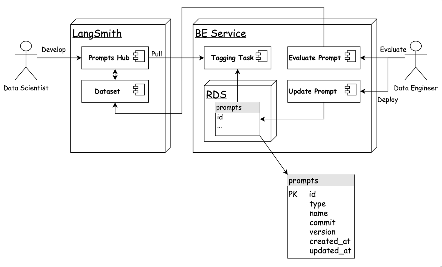
In our quest to facilitate swift experimentation with various prompt versions, we have empowered a diverse team of data scientists and engineers to work together effectively on the prompts and service. This has been made possible by upgrading our model architecture to incorporate the LangChain and LangSmith frameworks.
LangChain introduces a novel framework that streamlines the process from raw input to the desired outcome by chaining interoperable components. LangSmith, on the other hand, is a unified DevOps platform that fosters collaboration among various team members and developers, including product managers, data scientists, and software engineers. It simplifies the processes of development, collaboration, testing, deployment, and monitoring for all involved.
Our new backend leverages LangChain to construct an updated model that supports classification tasks for both non-PII and PII tagging. Integration with LangSmith enables data scientists to directly develop prompt templates and conduct experiments via the LangSmith user interface. In addition, managing the evaluation dataset on LangSmith provides a clear view of the performance of prompts across multiple custom metrics.
The integration of LangChain and LangSmith has significantly improved our model architecture, fostering collaboration and continuous improvement. This has not only streamlined our processes but also enhanced the transparency of our performance metrics. By harnessing the power of these innovative tools, we are better equipped to deliver high-quality, efficient solutions.
The benefits of the LangChain and LangSmith framework enhancements in Metasense are summarised as follows:
Streamlined prompt optimisation process.
Data scientists can create, update, and evaluate prompts directly on the LangSmith user interface and save them in commit mode. For rapid deployment, the prompt identifier in service configurations can be easily adjusted.
LangSmith’s capabilities allow us to effortlessly run evaluations on a dataset and obtain performance metrics across multiple dimensions, such as accuracy, latency, and error rate.
Assuring quality in perpetuity
With exceptionally low misclassification rates recorded, table owners can place greater trust in the model’s outputs and spend less time reviewing them. Nevertheless, as a prudent safety measure, we have set up alerts to monitor misclassification rates periodically, sounding an internal alarm if the rate crosses a defined threshold. A model improvement protocol has also been set in place for such alarms.
Conclusion
The integration of LLM into our metadata generation process has significantly improved our data classification capabilities, reducing manual workloads and increasing accuracy. Continuous improvements, including the adoption of LangChain and LangSmith frameworks, have streamlined prompt optimisation and enhanced collaboration among our team. With low misclassification rates and robust safety measures, our system is both reliable and scalable, fostering trust and efficiency. In conclusion, these advancements ensure we remain at the forefront of data governance, delivering high-quality solutions and valuable insights to our stakeholders.
We would like to express our sincere gratitude to Infocomm Media Development Authority (IMDA) for supporting this initative.
Join us
Grab is the leading superapp platform in Southeast Asia, providing everyday services that matter to consumers. More than just a ride-hailing and food delivery app, Grab offers a wide range of on-demand services in the region, including mobility, food, package and grocery delivery services, mobile payments, and financial services across 700 cities in eight countries.
Powered by technology and driven by heart, our mission is to drive Southeast Asia forward by creating economic empowerment for everyone. If this mission speaks to you, join our team today!
The Open Source Initiative has published (news article here) its definition of “open source AI,” and it’s terrible. It allows for secret training data and mechanisms. It allows for development to be done in secret. Since for a neural network, the training data is the source code—it’s how the model gets programmed—the definition makes no sense.
And it’s confusing; most “open source” AI models—like LLAMA—are open source in name only. But the OSI seems to have been co-opted by industry players that want both corporate secrecy and the “open source” label. (Here’s one rebuttal to the definition.)
This is worth fighting for. We need a publicAIoption, and open source—real open source—is a necessary component of that.
But while open source should mean open source, there are some partially open models that need some sort of definition. There is a big research field of privacy-preserving, federated methods of ML model training and I think that is a good thing. And OSI has a point here:
Why do you allow the exclusion of some training data?
Because we want Open Source AI to exist also in fields where data cannot be legally shared, for example medical AI. Laws that permit training on data often limit the resharing of that same data to protect copyright or other interests. Privacy rules also give a person the rightful ability to control their most sensitive information like decisions about their health. Similarly, much of the world’s Indigenous knowledge is protected through mechanisms that are not compatible with later-developed frameworks for rights exclusivity and sharing.
How about we call this “open weights” and not open source?
Data is the fuel for AI; modern data is even more important for generative AI and advanced data analytics, producing more accurate, relevant, and impactful results. Modern data comes in various forms: real-time, unstructured, or user-generated. Each form requires a different solution. AWS’s data journey began with Amazon Simple Storage Service (Amazon S3) in 2006, marking the start of cloud-based data storage at scale. Since then, AWS has expanded its data offerings to cover the entire data lifecycle, offering a comprehensive ecosystem of services designed to harness the full potential of modern data, from ingestion and storage to processing and analysis, supporting the entire lifecycle of AI-driven innovation.
In this blog post, we will cover some AWS use cases for modern data architectures, showing how AWS enables organizations to leverage the power of data and generative AI technologies.
This blog focuses on selecting the right database for generative AI applications and provide knowledge that can enhance your understanding, guide your decision making, and ultimately lead to more successful AI projects. Selecting the right database for generative AI applications is not just about storage; it significantly impacts performance, scalability, ease of integration, and overall effectiveness of the AI solution.
Figure 1. Diagram that shows the key steps in a RAG workflow
Adopting a data mesh architecture can enhance an organization’s ability to manage data effectively, leading to improved performance, innovation, and overall business success. In this guidance, you will discover some strategies to build data mesh solutions on AWS.
Figure 2. The data mesh organizes data into domains, where data are seen as quality products to expose for consumption
Amazon S3 is an object storage service that supports multiple use cases, including data architectures. Big data pipelines can use Amazon S3 to store input, output, and intermediate results. Machine learning systems use Amazon S3 to process application logs and build the datasets both for experimentation and for production model training. Given the importance of the service and the number of use cases that a foundational storage service can support, we want to share best practices, performance optimization, and cost optimization strategies to work with Amazon S3. This video shows how Anthropic designs its architecture around Amazon S3 in their data architecture.
Figure 3. Workloads with predictable patterns often have low retrieval rates for long periods of time after, so we can design to adopt cheaper storage classes for them
If you are curious about the underlying architecture of Amazon S3 and want to drill down into its internal design, you can watch the re:Invent video Dive deep on Amazon S3.
This is an AWS case study on how HPE Aruba Supply Chain successfully re-architected and deployed their data solution by adopting a modern data architecture on AWS. The new solution has helped Aruba integrate data from multiple sources, along with optimizing their cost, performance, and scalability. This has also allowed the Aruba Supply Chain leadership to receive in-depth and timely insights for better decision-making, thereby elevating the customer experience.
This workshop highlights advantage of adopting a modern data architecture on AWS. By integrating the flexibility of a data lake with specialized analytics services, organizations can significantly enhance their data-driven decision-making capabilities. We encourage everyone to explore how this architecture can streamline their analytics processes and support diverse use cases, from real-time insights to advanced machine learning. It’s an excellent opportunity to leverage modern data architecture.
Figure 5. Data architectures are fundamental to power use cases ranging from analytics to machine learning
Thanks for reading! In the next blog, we will cover some tips on how to get the best out of your developer experience on AWS. To revisit any of our previous posts or explore the entire series, visit the Let’s Architect! page.
We’re pleased to share a new collection of Code Club projects designed to introduce creators to the fascinating world of artificial intelligence (AI) and machine learning (ML). These projects bring the latest technology to your Code Club in fun and inspiring ways, making AI and ML engaging and accessible for young people. We’d like to thank Amazon Future Engineer for supporting the development of this collection.
The value of learning about AI and ML
By engaging with AI and ML at a young age, creators gain a clearer understanding of the capabilities and limitations of these technologies, helping them to challenge misconceptions. This early exposure also builds foundational skills that are increasingly important in various fields, preparing creators for future educational and career opportunities. Additionally, as AI and ML become more integrated into educational standards, having a strong base in these concepts will make it easier for creators to grasp more advanced topics later on.
What’s included in this collection
We’re excited to offer a range of AI and ML projects that feature both video tutorials and step-by-step written guides. The video tutorials are designed to guide creators through each activity at their own pace and are captioned to improve accessibility. The step-by-step written guides support creators who prefer learning through reading.
The projects are crafted to be flexible and engaging. The main part of each project can be completed in just a few minutes, leaving lots of time for customisation and exploration. This setup allows for short, enjoyable sessions that can easily be incorporated into Code Club activities.
The collection is organised into two distinct paths, each offering a unique approach to learning about AI and ML:
Machine learning with Scratch introduces foundational concepts of ML through creative and interactive projects. Creators will train models to recognise patterns and make predictions, and explore how these models can be improved with additional data.
The AI Toolkit introduces various AI applications and technologies through hands-on projects using different platforms and tools. Creators will work with voice recognition, facial recognition, and other AI technologies, gaining a broad understanding of how AI can be applied in different contexts.
Inclusivity is a key aspect of this collection. The projects cater to various skill levels and are offered alongside an unplugged activity, ensuring that everyone can participate, regardless of available resources. Creators will also have the opportunity to stretch themselves — they can explore advanced technologies like Adobe Firefly and practical tools for managing Ollama and Stable Diffusion models on Raspberry Pi computers.
Project examples
One of the highlights of our new collection is Chomp the cheese, which uses Scratch Lab’s experimental face recognition technology to create a game students can play with their mouth! This project offers a playful introduction to facial recognition while keeping the experience interactive and fun.
In Teach a machine, creators train a computer to recognise different objects such as fingers or food items. This project introduces classification in a straightforward way using the Teachable Machine platform, making the concept easy to grasp.
Apple vs tomato also uses Teachable Machine, but this time creators are challenged to train a model to differentiate between apples and tomatoes. Initially, the model exhibits bias due to limited data, prompting discussions on the importance of data diversity and ethical AI practices.
Dance detector allows creators to use accelerometer data from a micro:bit to train a model to recognise dance moves like Floss or Disco. This project combines physical computing with AI, helping creators explore movement recognition technology they may have experienced in familiar contexts such as video games.
Dinosaur decision tree is an unplugged activity where creators use a paper-based branching chart to classify different types of dinosaurs. This hands-on project introduces the concept of decision-making structures, where each branch of the chart represents a choice or question leading to a different outcome. By constructing their own decision tree, creators gain a tactile understanding of how these models are used in ML to analyse data and make predictions.
These AI projects are designed to support young people to get hands-on with AI technologies in Code Clubs and other non-formal learning environments. Creators can also enter one of their projects into Coolest Projects by taking a short video showing their project and any code used to make it. Their creation will then be showcased in the online gallery for people all over the world to see.
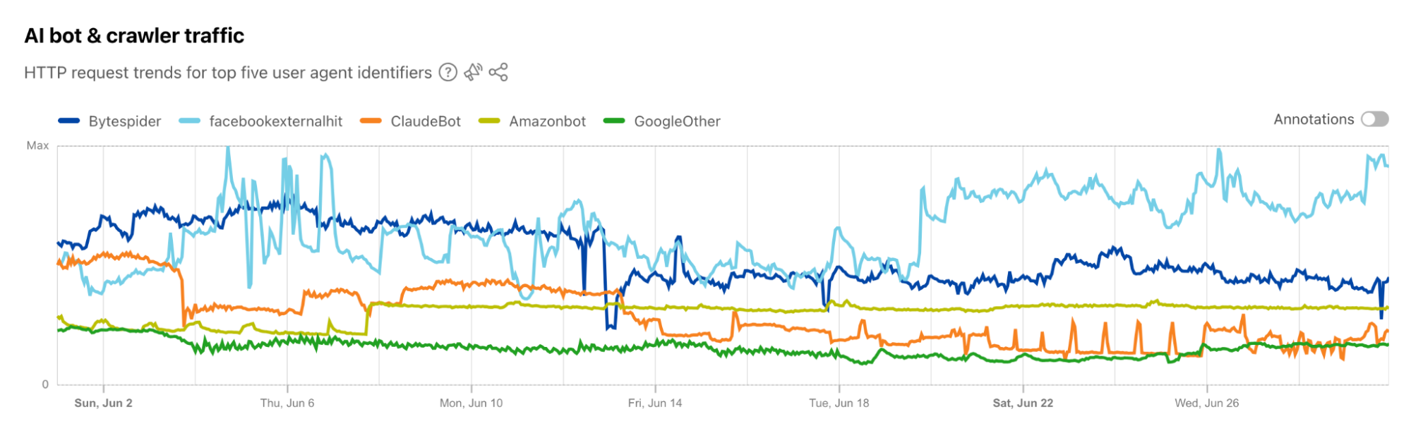
Our always-on DDoS protection runs inside every server across our global network. It constantly analyzes incoming traffic, looking for signals associated with previously identified DDoS attacks. We dynamically create fingerprints to flag malicious traffic, which is dropped when detected in high enough volume — so it never reaches its destination — keeping customer websites online.
In many cases, flagging bad traffic can be straightforward. For example, if we see too many requests to a destination with the same protocol violation, we can be fairly sure this is an automated script, rather than a surge of requests from a legitimate web browser.
Our DDoS systems are great at detecting attacks, but there’s a minor catch. Much like the human immune system, they are great at spotting attacks similar to things they have seen before. But for new and novel threats, they need a little help knowing what to look for, which is an expensive and time-consuming human endeavor.
Cloudflare protects millions of Internet properties, and we serve over 60 million HTTP requests per second on average, so trying to find unmitigated attacks in such a huge volume of traffic is a daunting task. In order to protect the smallest of companies, we need a way to find unmitigated attacks that may only be a few thousand requests per second, as even these can be enough to take smaller sites offline.
To better protect our customers, we also have a system to automatically identify unmitigated, or partially mitigated DDoS attacks, so we can better shore up our defenses against emerging threats. In this post we will introduce this anomaly detection pipeline, we’ll provide an overview of how it builds statistical models which flag unusual traffic and keep our customers safe. Let’s jump in!
A naive volumetric model
A DDoS attack, by definition, is characterized by a higher than normal volume of traffic destined for a particular destination. We can use this fact to loosely sketch out a potential approach. Let’s look at an example website, and look at the request volume over the course of a day, broken down into 1 minute intervals.
We can plot this same data as a histogram:
The data follows a bell-shaped curve, also known as a normal distribution. We can use this fact to flag observations which appear outside the usual range. By first calculating the mean and standard deviation of our dataset, we can then use these values to rate new observations by calculating how many standard deviations (or sigma) the data is from the mean.
This value is also called the z-score — a z-score of 3 is the same as 3-sigma, which corresponds to 3 standard deviations from the mean. A data point with a high enough z-score is sufficiently unusual that it might signal an attack. Since the mean and standard deviation are stationary, we can calculate a request volume threshold for each z-score value, and use traffic volumes above these thresholds to signal an ongoing attack.
Trigger thresholds for z-score of 3, 4 and 5
Unfortunately, it’s incredibly rare to see traffic that is this uniform in practice, as user load will naturally vary over a day. Here I’ve simulated some traffic for a website which runs a meal delivery service, and as you might expect it has big peaks around meal times, and low traffic overnight since it only operates in a single country.
Our volume data no longer follows a normal distribution and our 3-sigma threshold is now much further away, so smaller attacks could pass undetected.
Many websites elastically scale their underlying hardware based upon anticipated load to save on costs. In the example above the website operator would run far fewer servers overnight, when the anticipated load is low, to save on running costs. This makes the website more vulnerable to attacks during off-peak hours as there would be less hardware to absorb them. An attack as low as a few hundred requests per minute may be enough to overwhelm the site early in the morning, even though the peak-time infrastructure could easily absorb this volume.
This approach relies on traffic volume being stable over time, meaning it’s roughly flat throughout the day, but this is rarely true in practice. Even when it is true, benign increases in traffic are common, such as an e-commerce site running a Black Friday sale. In this situation, a website would expect a surge in traffic that our model wouldn’t anticipate, and we may incorrectly flag real shoppers as attackers.
It turns out this approach makes too many naive assumptions about what traffic should look like, so it’s impossible to choose an appropriate sigma threshold which works well for all customers.
Time series forecasting
Let’s continue with trying to determine a volumetric baseline for our meal delivery example. A reasonable assumption we could add is that yesterday’s traffic shape should approximate the expected shape of traffic today. This idea is called “seasonality”. Weekly seasonality is also pretty common, i.e. websites see more or less traffic on certain weekdays or on weekends.
There are many methods designed to analyze a dataset, unpick the varying horizons of seasonality within it, and then build an appropriate predictive model. We won’t go into them here but reading about Seasonal ARIMA (SARIMA) is a good place to start if you are looking for further information.
There are three main challenges that make SARIMA methods unsuitable for our purposes. First is that in order to get a good idea of seasonality, you need a lot of data. To predict weekly seasonality, you need at least a few weeks worth of data. We’d require a massive dataset to predict monthly, or even annual, patterns (such as Black Friday). This means new customers wouldn’t be protected until they’d been with us for multiple years, so this isn’t a particularly practical approach.
The second issue is the cost of training models. In order to maintain good accuracy, time series models need to be frequently retrained. The exact frequency varies between methods, but in the worst cases, a model is only good for 2–3 inferences, meaning we’d need to retrain all our models every 10–20 minutes. This is feasible, but it’s incredibly wasteful.
The third hurdle is the hardest to work around, and is the reason why a purely volumetric model doesn’t work. Most websites experience completely benign spikes in traffic that lie outside prior norms. Flash sales are one such example, or 1,000,000 visitors driven to a site from Reddit, or a Super Bowl commercial.
A better way?
So if volumetric modeling won’t work, what can we do instead? Fortunately, volume isn’t the only axis we can use to measure traffic. Consider the end users’ browsers for example. It would be reasonable to assume that over a given time interval, the proportion of users across the top 5 browsers would remain reasonably stationary, or at least within a predictable range. More importantly, this proportion is unlikely to change too much during benign traffic surges.
Through careful analysis we were able to discover about a dozen such variables with the following features for a given zone:
They follow a normal distribution
They aren’t correlated, or are only loosely correlated with volume
They deviate from the underlying normal distribution during “under attack” events
Recall our initial volume model, where we used z-score to define a cutoff. We can expand this same idea to multiple dimensions. We have a dozen different time series (each feature is a single time series), which we can imagine as a cloud of points in 12 dimensions. Here is a sample showing 3 such features, with each point representing the traffic readings at a different point in time. Note that both graphs show the same cloud of points from two different angles.
To use our z-score analogy from before, we’d want our points to be spherical, since our multidimensional- z-score is then just the distance from the centre of the cloud. We could then use this distance to define a cutoff threshold for attacks.
For several reasons, a perfect sphere is unlikely in practice. Our various features measure different things, so they have very different scales of ‘normal’. One property might vary between 100-300 whereas another property might usually occupy the interval 0-1. A change of 3 in this latter property would be a significant anomaly, whereas in the first this would just be within the normal range.
More subtly, two or more axes may be correlated, so an increase in one is usually mirrored with a proportional increase/decrease in another dimension. This turns our sphere into an off-axis disc shape, as pictured above.
Fortunately, we have a couple of mathematical tricks up our sleeve. The first is scale normalization. In each of our n dimensions, we subtract the mean, and divide by the standard deviation. This makes all our dimensions the same size and centres them around zero. This gives a multidimensional analogue of z-score, but it won’t fix the disc shape.
What we can do is figure out the orientation and dimensions of the disc, and for this we use a tool called Principal Component Analysis (PCA). This lets us reorient our disc, and rescale the axes according to their size, to make them all the same.
Imagine grabbing the disc out of the air, then drawing new X and Y axes on the top surface, with the origin at the center of the disc. Our new Z-axis is the thickness of the disc. We can compare the thickness to the diameter of the disc, to give us a scaling factor for the Z direction. Imagine stretching the disc along the z-axis until it’s as tall as the length across the diameter.
In reality there’s nothing to say that X & Y have to be the same size either, but hopefully you get the general idea. PCA lets us draw new axes along these lines of correlation in an arbitrary number of dimensions, and convert our n-dimensional disc into a nicely behaved sphere of points (technically an n-dimensional sphere).
Having done all this work, we can uniquely define a coordinate transformation which takes any measurement from our raw features, and tells us where it should lie in the sphere, and since all our dimensions are the same size we can generate an anomaly score purely based on its distance from the centre of the cloud.
As a final trick, we can also use a final scaling operation to ensure the sphere for dataset A is the same size as the sphere generated from dataset B, meaning we can do this same process for any traffic data and define a cutoff distance λ which is the same across all our models. Rather than fine-tuning models for each individual customer zone, we can tune this to a value which applies globally.
Another name for this measurement is Mahalanobis distance. (Inclined readers can understand this equivalence by considering the role of the covariance matrix in PCA and Mahalanobis distance. Further discussion can be found on this StackExchange post.) We further tune the process to discard dimensions with little variance — if our disc is too thin we discard the thickness dimension. In practice, such dimensions were too sensitive to be useful.
We’re left with a multidimensional analogue of the z-score we started with, but this time our variables aren’t correlated with peacetime traffic volume. Above we show 2 output dimensions, with coloured circles which show Mahalanobis distances of 4, 5 and 6. Anything outside the green circle will be classified as an attack.
How we train ~1 million models daily to keep customers safe
The approach we’ve outlined is incredibly parallelizable: a single model requires only the traffic data for that one website, and the datasets needed can be quite small. We use 4 weeks of training data chunked into 5 minute intervals which is only ~8k rows/website.
We run all our training and inference in an Apache Airflow deployment in Kubernetes. Due to the parallelizability, we can scale horizontally as needed. On average, we can train about 3 models/second/thread. We currently retrain models every day, but we’ve observed very little intraday model drift (i.e. yesterday’s model is the same as today’s), so training frequency may be reduced in the future.
We don’t consider it necessary to build models for all our customers, instead we train models for a large sample of representative customers, including a large number on the Free plan. The goal is to identify attacks for further study which we then use to tune our existing DDoS systems for all customers.
Join us!
If you’ve read this far you may have questions, like “how do you filter attacks from your training data?” or you may have spotted a handful of other technical details which I’ve elided to keep this post accessible to a general audience. If so, you would fit in well here at Cloudflare. We’re helping to build a better Internet, and we’re hiring.
As the complexity of data retrieval requirements continue to grow, traditional search methods often struggle to provide relevant and accurate results, especially for nuanced or conceptual queries. Vector similarity search has emerged as a powerful technique for finding semantically similar information. It refers to finding vectors in a large dataset that are most similar to a given query vector, typically using some distance or similarity measure. The concept originated in the 1960s with the work by Minsky and Papert on nearest neighbour search 1. Since then, the idea has evolved substantially with modern approaches often using approximate methods to enable fast search in high-dimensional spaces, such as locality-sensitive hashing 2 and graph-based indexing 3.
Recently, vector similarity search has become a crucial component in many machine learning and information retrieval applications. It is one of the key technologies that popularised the idea of Retrieval Augmented Generation (RAG) 4 which increased the applicability of Transformer 5 based Generative Large Language Models (LLMs) 6 in domain-specific tasks without requiring any further training or fine-tuning. However, the effectiveness of the vector search can be limited when dealing with intricate queries or contextual nuances. For example, from a typical vector similarity search perspective, “I like fishing” and “I do not like fishing” may be quite close to each other, while in reality, they are the exact opposite. In this blog post, we discuss an approach that we experimented with that combines vector similarity search with LLMs to enhance the relevance and accuracy of search results for such complex and nuanced queries. We leverage the strengths of both techniques: vector similarity search for efficient shortlisting of potential matches, and LLMs for their ability to understand natural language queries and rank the shortlisted results based on their contextual relevance.
Proposed solution
The proposed solution involves a two-step process:
Vector similarity search: We first perform a vector similarity search on the dataset to obtain a shortlist of potential matches (e.g., top 10-50 results) for the given query. This step leverages the efficiency of vector similarity search to quickly narrow down the search space.
LLM-assisted ranking: The shortlisted results from the vector similarity search are then fed into an LLM, which ranks the results based on their relevance to the original query. The LLM’s ability to understand natural language queries and contextual information helps in identifying the most relevant results from the shortlist.
By combining these two steps, we aim to achieve the best of both worlds: the efficiency of vector similarity search for initial shortlisting, and the contextual understanding and ranking capabilities of LLMs for refining the final results.
Figure 1. Similarity search and the proposed LLM-assisted similarity search.
Experiment
Datasets
To evaluate the effectiveness of our proposed solution, we conducted experiments on two small synthetic datasets in CSV format that we curated using GPT-4o 7.
Food dataset: A collection of 100 dishes with their titles and descriptions.
Tourist spots dataset: A collection of 100 tourist spots in Asia, including their names, cities, countries, and descriptions.
It is important to note that we primarily focus on performing similarity search on structured data such as description of various entities in a relational database.
Setup
Our experimental setup included a Python script for vector similarity search leveraging Facebook AI Similarity Search (FAISS) 8, a library developed by Facebook that offers efficient similarity search, and OpenAI’s embeddings (i.e., text-embedding-ada-002) 9 to generate the vector embeddings needed for facilitating the vector search. For our proposed solution, an LLM component (i.e., GPT-4o) was included in the setup in addition to the FAISS-based similarity search component.
Observations
To compare the performance of the proposed approach of LLM-assisted vector similarity search as outlined in the “Proposed solution” section with the raw vector similarity search, we conducted both techniques on our two synthetic datasets. With the raw vector search, we get the top three matches for a given query. For our proposed technique, we first get a shortlist of 15 entity matches from FAISS for the same query, and supply the shortlist and the original query to LLM with some descriptive instructions in the prompt to find the top three matches from the provided shortlist.
From the experiments, in simpler cases where the queries were straightforward and directly aligned with the textual content of the data, both the raw similarity search and the LLM-assisted similarity search demonstrated comparable performance. However, as the queries became more complex, involving additional constraints, negations, or conceptual requirements, the LLM-assisted search exhibited a clear advantage over the raw similarity search. The LLM’s ability to understand context and capture subtleties in the queries allowed it to filter out irrelevant results and rank the most appropriate ones higher, leading to improved accuracy.
Here are a few examples where the LLM-assisted similarity search performed better:
Food dataset
Query: “food with no fish or shrimp”
Raw similarity search result:
- title: Tempura, description: A Japanese dish of seafood or vegetables that have been battered and deep fried.
- title: Ceviche, description: A seafood dish popular in Latin America, made from fresh raw fish cured in citrus juices.
- title: Sushi, description: A Japanese dish consisting of vinegared rice accompanied by various ingredients such as seafood and vegetables.
LLM-assisted similarity search result:
- title: Chicken Piccata, description: Chicken breasts cooked in a sauce of lemon, butter, and capers.
- title: Chicken Alfredo, description: An Italian-American dish of pasta in a creamy sauce made from butter and Parmesan cheese.
- title: Chicken Satay, description: Grilled chicken skewers served with peanut sauce.
Observation: The LLM correctly filtered out dishes containing fish or shrimp, while the raw similarity search failed to do so, presumably due to the presence of negation in the query.
Tourist spots dataset
Query: “exposure to wildlife”
Raw similarity search result:
- name: Ocean Park, city: Hong Kong, country: Hong Kong, description: Marine mammal park and oceanarium.
- name: Merlion Park, city: Singapore, country: Singapore, description: Iconic statue with the head of a lion and body of a fish.
- name: Manila Bay, city: Manila, country: Philippines, description: A natural harbor known for its sunset views.
LLM-assisted similarity search result:
- name: Ocean Park, city: Hong Kong, country: Hong Kong, description: Marine mammal park and oceanarium.
- name: Chengdu Research Base, city: Chengdu, country: China, description: A research center for giant panda breeding.
- name: Mount Hua, city: Shaanxi, country: China, description: Mountain known for its dangerous hiking trails.
Observation: Two out of the top three matches by the LLM-assisted technique seem relevant to the query while only one result from the raw similarity search is relevant and the other two being somewhat irrelevant to the query. The LLM identified the relevance of a research base for giant panda breeding to the “exposure to wildlife”, which the raw similarity search ignored in its ranking.
These examples provide a glimpse into the utility of LLMs in finding more relevant matches in scenarios where the queries involved additional context, constraints, or conceptual requirements beyond simple keyword matching. On the other hand, when the queries were more straightforward and focused on specific keywords or phrases present in the data, both approaches demonstrated comparable performance. For instance, queries like “Japanese food” or “beautiful mountains” yielded similar results from both the raw similarity search and the proposed LLM-assisted approach.
Overall, the LLM-assisted vector search exhibited a clear advantage in handling complex queries, leveraging its ability to understand natural language and contextual information. However, for simpler queries, the raw similarity search remained a viable option, especially when computational efficiency is a concern.
Conclusion
The experiments demonstrated the potential of combining vector similarity search with LLMs to enhance the relevance and accuracy of search results, particularly for complex and nuanced queries. While vector similarity search alone can provide reasonable results for straightforward queries, the LLM-assisted approach shines when dealing with queries that require a deeper understanding of context, nuances, and conceptual relationships. By leveraging the natural language understanding capabilities of LLMs, this approach can better capture the intent behind complex queries and provide more relevant search results.
Our experiment was limited to using a small volume of structured data (100 data points in each dataset) with a limited number of queries. However, we have witnessed similar enhancement in search result relevance when we deployed this solution internally within Grab for larger datasets, for example, 4500+ rows of data stored in a relational database.
Nevertheless, it is important to note that the effectiveness of this approach may still depend on the quality and complexity of the data, as well as the specific use case and query patterns. We believe it is still worthwhile to evaluate the proposed approach for more diverse (e.g., beyond CSV) and larger datasets. An interesting future work can be varying the size of the shortlist from the similarity search and observing how it impacts the overall search relevance when using the proposed approach. In addition, for real world applications, the performance implications in terms of additional latency introduced by the additional LLM query must also be considered.
Join us
Grab is the leading superapp platform in Southeast Asia, providing everyday services that matter to consumers. More than just a ride-hailing and food delivery app, Grab offers a wide range of on-demand services in the region, including mobility, food, package and grocery delivery services, mobile payments, and financial services across 700 cities in eight countries.
Powered by technology and driven by heart, our mission is to drive Southeast Asia forward by creating economic empowerment for everyone. If this mission speaks to you, join our team today!
References
M. Minsky and S. Papert, Perceptrons: An Introduction to Computational Geometry. MIT Press, 1969. ↩
P. Indyk and R. Motwani, “Approximate nearest neighbors: Towards removing the curse of dimensionality,” in Proceedings of the Thirtieth Annual ACM Symposium on Theory of Computing, 1998. ↩
Y. Malkov and D. Yashunin, “Efficient and robust approximate nearest neighbor search using hierarchical navigable small world graphs,” IEEE Transactions on Pattern Analysis and Machine Intelligence, 2020. ↩
P. Lewis, E. Perez, A. Piktus, F. Petroni, V. Karpukhin, N. Goyal, and D. Kiela, “Retrieval-augmented generation for knowledge-intensive NLP tasks,” in Advances in Neural Information Processing Systems, 2020. ↩
A. Vaswani, “Attention is all you need,” in Advances in Neural Information Processing Systems, 2017. ↩
A. Radford, “Improving language understanding by generative pre-training,” 2018. ↩
Retrieval-Augmented Generation (RAG) is a powerful process that is designed to integrate direct function calling to answer queries more efficiently by retrieving relevant information from a broad database. In the rapidly evolving business landscape, Data Analysts (DAs) are struggling with the growing number of data queries from stakeholders. The conventional method of manually writing and running similar queries repeatedly is time-consuming and inefficient. This is where RAG-powered Large Language Models (LLMs) step in, offering a transformative solution to streamline the analytics process and empower DAs to focus on higher value tasks.
In this article, we will share how the Integrity Analytics team has built out a data solution using LLMs to help automate tedious analytical tasks like generating regular metric reports and performing fraud investigations.
While LLMs are known for their proficiency in data interpretation and insight generation, they represent just a fragment of the entire solution. For a comprehensive solution, LLMs must be integrated with other essential tools. The following is required in assembling a solution:
Internally facing LLM tool – Spellvault is a platform within Grab that stores, shares, and refines LLM prompts. It features low/no-code RAG capabilities that lower the barrier of entry for people to create LLM applications.
Data – with real time or close to real-time latency to ensure accuracy. It has to be in a standardised format to ensure that all LLM data inputs are accurate.
Scheduler – runs LLM applications at regular intervals. Useful for automating routine tasks.
Messaging Tool – a user interface where users can interact with LLM by entering a command to receive reports and insights.
Introducing Data-Arks, the data middleware serving up relevant data to the LLM agents
For most data use cases, DAs are usually running the same set of SQL queries with minor changes to parameters like dates, age or other filter conditions. In most instances, we already have a clear understanding of the required data and format to accomplish a task. Therefore, we need a tool that can execute the exact SQL query and channel the data output to the LLM.
Figure 1. Data-Arks hosts various APIs which can be called to serve data to applications like SpellVault.
What is Data-Arks?
Data-Arks is an in-house Python-based API platform housing several frequently used SQL queries and python functions packaged into individual APIs. Data-Arks is also integrated with Slack, Wiki, and JIRA APIs, allowing users to parse and fetch information and data from these tools as well. The benefits of Data-Arks are summarised as follows:
Integration: Data-Arks service allows users to upload any SQL query or Python script on the platform. These queries are then surfaced as APIs, which can be called to serve data to the LLM agent.
Versatility: Data-Arks can be extended to everyone. Employees from various teams and functions at Grab can self-serve to upload any SQL query that they want onto the platform, allowing this tool to be used for different teams’ use cases.
Automating regular report generation and summarisation using Data-Arks and Spellvault
LLMs are just one piece of the puzzle, to build a comprehensive solution, they must be integrated with other tools. Figure 2 shows how different tools are used in executing report summaries in Slack.
Figure 2 shows how different tools are used in executing report summaries in Slack.
Figure 2. Report Summarizer uses various tools to summarise queries and deliver a summarised report through Slack.
Figure 3 is an example of a summarised report generated by the Report Summarizer using dummy data. Report Summarizer calls a Data-Arks API to generate the data in a tabular format and LLM helps summarise and generate a short paragraph of key insights. This automated report generation has helped save an estimated 3-4 hours per report.
Figure 3. Sample of a report generated using dummy data extracted from [https://data.gov.my/](https://data.gov.my/).
LLM bots for fraud investigations
LLMs also excel in helping to streamline fraud investigations, as LLMs are able to contextualise several different data points and information and derive useful insights from them.
Introducing A* bot, the team’s very own LLM fraud investigation helper.
A set of frequently used queries for fraud investigation is made available as Data-Arks APIs. Upon a user prompt or query, SpellVault selects the most relevant queries using RAG, executes them and provides a summary of the results to users through Slack.
Figure 4. A* bot uses Data-Arks and Spellvault to get information for fraud investigations.
Figure 5 shows a sample of fraud investigation responses from A* bot. Scaling to multiple queries for a fraud investigation process, what was once a time-consuming fraud investigation can now be reduced to a matter of minutes, as the A* bot is capable of providing all the necessary information simultaneously.
Figure 5. Sample of fraud investigation responses.
RAG vs fine-tuning
On deciding between RAG or fine-tuning to improve LLM accuracy, three key factors tipped the scales in favour of the RAG approach:
Effort and cost considerations
Fine-tuning requires significant computational cost as it involves taking a base model and further training it with smaller, domain specific data and context. RAG is computationally less expensive as it relies on retrieving only relevant data and context to augment a model’s response. As the same base model can be used for different use cases, RAG is the preferred choice due to its flexibility and cost efficiency.
Ability to respond with the latest information
Fine-tuning requires model re-training with each new information update, whereas RAG simply retrieves required context and data from a knowledge base to enhance its response. Thus, by using RAG, LLM is able to answer questions using the most current information from our production database, eliminating the need for model re-training.
Speed and scalability
Without the burden of model re-training, the team can rapidly scale and build out new LLM applications with a well managed knowledge base.
What’s next?
The potential of using RAG-powered LLM can be limitless as the ability of GPT is correlated with the tools it equips. Hence, the process does not stop here and we will try to onboard more tools or integration to GPT. In the near future, we plan to utilise Data-Arks to provide images to GPT as GPT-4o is a multimodal model that has vision capabilities. We are committed to pushing the boundaries of what’s possible with RAG-powered LLM, and we look forward to unveiling the exciting advancements that lie ahead.
Figure 6. What’s next?
We would like to express our sincere gratitude to the following individuals and teams whose invaluable support and contributions have made this project a reality: – Meichen Lu, a senior data scientist at Grab, for her guidance and assistance in building the MVP and testing the concept. – The data engineering team, particularly Jia Long Loh and Pu Li, for setting up the necessary services and infrastructure.
Join us
Grab is the leading superapp platform in Southeast Asia, providing everyday services that matter to consumers. More than just a ride-hailing and food delivery app, Grab offers a wide range of on-demand services in the region, including mobility, food, package and grocery delivery services, mobile payments, and financial services across 700 cities in eight countries.
Powered by technology and driven by heart, our mission is to drive Southeast Asia forward by creating economic empowerment for everyone. If this mission speaks to you, join our team today!
As Southeast Asia’s leading super app, Grab serves millions of users across multiple countries every day. Our services range from ride-hailing and food delivery to digital payments and much more. The backbone of our operations? Machine Learning (ML) models. They power our real-time decision-making capabilities, enabling us to provide a seamless and personalised experience to our users. Whether it’s determining the most efficient route for a ride, suggesting a food outlet based on a user’s preference, or detecting fraudulent transactions, ML models are at the forefront.
However, serving these ML models at Grab’s scale is no small feat. It requires a robust, efficient, and scalable model serving platform, which is where our ML model serving platform, Catwalk, comes in.
Catwalk has evolved over time, adapting to the growing needs of our business and the ever-changing tech landscape. It has been a journey of continuous learning and improvement, with each step bringing new challenges and opportunities.
Evolution of the platform
Phase 0: The need for a model serving platform
Before Catwalk’s debut as our dedicated model serving platform, data scientists across the company employed various ad-hoc approaches to serve ML models. These included:
Shipping models online using custom solutions.
Relying on backend engineering teams to deploy and manage trained ML models.
Embedding ML logic within Go backend services.
These methods, however, led to several challenges, undercovering the need for a unified, company-wide platform for serving machine learning models:
Operational overhead: Data scientists often lacked the necessary expertise to handle the operational aspects of their models, leading to service outages.
Resource wastage: There was frequently low resource utilisation (e.g., 1%) for data science services, leading to inefficient use of resources.
Friction with engineering teams: Differences in release cycles and unclear ownership when code was embedded into backend systems resulted in tension between data scientists and engineers.
Reinventing the wheel: Multiple teams independently attempted to solve model serving problems, leading to a duplication of effort.
These challenges highlighted the need for a company-wide, centralised platform for serving machine learning models.
Phase 1: No-code, managed platform for TensorFlow Serving models
Our initial foray into model serving was centred around creating a managed platform for deploying TensorFlow Serving models. The process involved data scientists submitting their models to the platform’s engineering admin, who could then deploy the model with an endpoint. Infrastructure and networking were managed using Amazon Elastic Kubernetes Service (EKS) and Helm Charts as illustrated below.
This phase of our platform, which we also detailed in our previous article, was beneficial for some users. However, we quickly encountered scalability challenges:
Codebase maintenance: Applying changes to every TensorFlow Serving (TFS) version was cumbersome and difficult to maintain.
Limited scalability: The fully managed nature of the platform made it difficult to scale.
Admin bottleneck: The engineering admin’s limited bandwidth became a bottleneck for onboarding new models.
Limited serving types: The platform only supported TensorFlow, limiting its usefulness for data scientists using other frameworks like LightGBM, XGBoost, or PyTorch.
After a year of operation, only eight models were onboarded to the platform, highlighting the need for a more scalable and flexible solution.
Phase 2: From models to model serving applications
To address the limitations of Phase 1, we transitioned from deploying individual models to self-contained model serving applications. This “low-code, self-serving” strategy introduced several new components and changes as illustrated in the points and diagram below:
Support for multiple serving types: Users gained the ability to deploy models trained with a variety of frameworks like Open Neural Network Exchange (ONNX), PyTorch, and TensorFlow.
Self-served platform through CI/CD pipelines: Data scientists could self-serve and independently manage their model serving applications through CI/CD pipelines.
New components: We introduced these new components to support the self-serving approach:
Catwalk proxy, a managed reverse proxy to various serving types.
Catwalk transformer, a low-code component to transform input and output data.
Amphawa, a feature fetching component to augment model inputs.
API request flow
The Catwalk proxy acts as the orchestration layer. Clients send requests to Catwalk proxy then it orchestrates calls to different components like transformers, feature-store, and so on. A typical end to end request flow is illustrated below.
Within a year of implementing these changes, the number of models on the platform increased from 8 to 300, demonstrating the success of this approach. However, new challenges emerged:
Complexity of maintaining Helm chart: As the platform continued to grow with new components and functionalities, maintaining the Helm chart became increasingly complex. The readability and flow control became more challenging, making the helm chart updating process prone to errors.
Process-level mistakes: The self-serving approach led to errors such as pushing empty or incompatible models to production, setting too few replicas, or allocating insufficient resources, which resulted in service crashes.
We knew that our work was nowhere near done. We had to keep iterating and explore ways to address the new challenges.
Phase 3: Replacing Helm charts with Kubernetes CRDs
To tackle the deployment challenges and gain more control, we made the significant decision to replace Helm charts with Kubernetes Custom Resource Definitions (CRDs). This required substantial engineering effort, but the outcomes have been rewarding. This transition gave us improved control over deployment pipelines, enabling customisations such as:
Smart defaults for AutoML
Blue-green deployments
Capacity management
Advanced scaling
Application set groupings
Below is an example of a simple model serving CRD manifest:
Every model serving CRD submission follows a sequence of steps. If there are failures at any step, the controller keeps retrying after small intervals. The major steps on the deployment cycle are described below:
Validate whether the new CRD specs are acceptable. Along with sanity checks, we also enforce a lot of platform constraints through this step.
Clean up previous non-ready deployment resources. Sometimes a deployment submission might keep crashing and hence it doesn’t proceed to a ready state. On every submission, it’s important to check and clean up such previous deployments.
Create resources for the new deployment and ensure that the new deployment is ready.
Switch traffic from old deployment to the new deployment.
Clean up resources for old deployment. At this point, traffic is already being served by the new deployment resources. So, we can clean up the old deployment.
Phase 4: Transition to a high-code, self-served, process-managed platform
As the number of model serving applications and use cases multiplied, clients sought greater control over orchestrations between different models, experiment executions, traffic shadowing, and responses archiving. To cater to these needs, we introduced several changes and components with the Catwalk Orchestrator, a high code orchestration solution, leading the pack.
Catwalk orchestrator
The Catwalk Orchestrator is a highly abstracted framework for building ML applications that replaced the catwalk-proxy from previous phases. The key difference is that users can now write their own business/orchestration logic. The orchestrator offers a range of utilities, reducing the need for users to write extensive boilerplate code. Key components of the Catwalk Orchestrator include HTTP server, gRPC server, clients for different model serving flavours (TensorFlow, ONNX, PyTorch, etc), client for fetching features from the feature bank, and utilities for logging, metrics, and data lake ingestion.
The Catwalk Orchestrator is designed to streamline the deployment of machine learning models. Here’s a typical user journey:
Scaffold a model serving application: Users begin by scaffolding a model serving application using a command-line tool.
Write business logic: Users then write the business logic for the application.
Deploy to staging: The application is then deployed to a staging environment for testing.
Complete load testing: Users test the application in the staging environment and complete load testing to ensure it can handle the expected traffic.
Deploy to production: Once testing is completed, the application is deployed to the production environment.
Bundled deployments
To support multiple ML models as part of a single model serving application, we introduced the concept of bundled deployments. Multiple Kubernetes deployments are bundled together as a single model serving application deployment, allowing each component (e.g., models, catwalk-orchestrator, etc) to have its own Kubernetes deployment and to scale independently.
In addition to the major developments, we implemented other changes to enhance our platform’s efficiency. We made load testing mandatory for all ML application updates to ensure robust performance. This testing process was streamlined with a single command that runs the load test in the staging environment, with the results directly shared with the user.
Furthermore, we boosted deployment transparency by sharing deployment details through Slack and Datadog. This empowered users to diagnose issues independently, reducing the dependency on on-call support. This transparency not only improved our issue resolution times but also enhanced user confidence in our platform.
The results of these changes speak for themselves. The Catwalk Orchestrator has evolved into our flagship product. In just two years, we have deployed 200 Catwalk Orchestrators serving approximately 1,400 ML models.
What’s next?
As we continue to innovate and enhance our model serving platform, we are venturing into new territories:
Catwalk serverless: We aim to further abstract the model serving experience, making it even more user-friendly and efficient.
Catwalk data serving: We are looking to extend Catwalk’s capabilities to serve data online, providing a more comprehensive service.
LLM serving: In line with the trend towards generative AI and large language models (LLMs), we’re pivoting Catwalk to support these developments, ensuring we stay at the forefront of the AI and machine learning field.
Stay tuned as we continue to advance our technology and bring these exciting developments to life.
Join us
Grab is the leading superapp platform in Southeast Asia, providing everyday services that matter to consumers. More than just a ride-hailing and food delivery app, Grab offers a wide range of on-demand services in the region, including mobility, food, package and grocery delivery services, mobile payments, and financial services across 700 cities in eight countries.
Powered by technology and driven by heart, our mission is to drive Southeast Asia forward by creating economic empowerment for everyone. If this mission speaks to you, join our team today!
The continued growth of AI has fundamentally changed the Internet over the past 24 months. AI is increasingly ubiquitous, and Cloudflare is leaning into the new opportunities and challenges it presents in a big way. This year for Cloudflare’s birthday, we’ve extended our AI Assistant capabilities to help you build new WAF rules, added AI bot traffic insights on Cloudflare Radar, and given customers new AI bot blocking capabilities.
AI Assistant for WAF Rule Builder
At Cloudflare, we’re always listening to your feedback and striving to make our products as user-friendly and powerful as possible. One area where we’ve heard your feedback loud and clear is in the complexity of creating custom and rate-limiting rules for our Web Application Firewall (WAF). With this in mind, we’re excited to introduce a new feature that will make rule creation easier and more intuitive: the AI Assistant for WAF Rule Builder.
By simply entering a natural language prompt, you can generate a custom or rate-limiting rule tailored to your needs. For example, instead of manually configuring a complex rule matching criteria, you can now type something like, “Match requests with low bot score,” and the assistant will generate the rule for you. It’s not about creating the perfect rule in one step, but giving you a strong foundation that you can build on.
The assistant will be available in the Custom and Rate Limit Rule Builder for all WAF users. We’re launching this feature in Beta for all customers, and we encourage you to give it a try. We’re looking forward to hearing your feedback (via the UI itself) as we continue to refine and enhance this tool to meet your needs.
AI bot traffic insights on Cloudflare Radar
AI platform providers use bots to crawl and scrape websites, vacuuming up data to use for model training. This is frequently done without the permission of, or a business relationship with, the content owners and providers. In July, Cloudflare urged content owners and providers to “declare their AIndependence”, providing them with a way to block AI bots, scrapers, and crawlers with a single click. In addition to this so-called “easy button” approach, sites can provide more specific guidance to these bots about what they are and are not allowed to access through directives in a robots.txt file. Regardless of whether a customer chooses to block or allow requests from AI-related bots, Cloudflare has insight into request activity from these bots, and associated traffic trends over time.
Tracking traffic trends for AI bots can help us better understand their activity over time — which are the most aggressive and have the highest volume of requests, which launch crawls on a regular basis, etc. The new AI bot & crawler traffic graph on Radar’s Traffic page provides insight into these traffic trends gathered over the selected time period for the top known AI bots. The associated list of bots tracked here is based on the ai.robots.txt list, and will be updated with new bots as they are identified. Time series and summary data is available from the Radar API as well. (Traffic trends for the full set of AI bots & crawlers can be viewed in the new Data Explorer.)
Blocking more AI bots
For Cloudflare’s birthday, we’re following up on our previous blog post, Declaring Your AIndependence, with an update on the new detections we’ve added to stop AI bots. Customers who haven’t already done so can simply click the button to block AI bots to gain more protection for their website.
Enabling dynamic updates for the AI bot rule
The old button allowed customers to block verified AI crawlers, those that respect robots.txt and crawl rate, and don’t try to hide their behavior. We’ve added new crawlers to that list, but we’ve also expanded the previous rule to include 27 signatures (and counting) of AI bots that don’t follow the rules. We want to take time to say “thank you” to everyone who took the time to use our “tip line” to point us towards new AI bots. These tips have been extremely helpful in finding some bots that would not have been on our radar so quickly.
For each bot we’ve added, we’re also adding them to our “Definitely automated” definition as well. So, if you’re a self-service plan customer using Super Bot Fight Mode, you’re already protected. Enterprise Bot Management customers will see more requests shift from the “Likely Bot” range to the “Definitely automated” range, which we’ll discuss more below.
Under the hood, we’ve converted this rule logic to a Cloudflare managed rule (the same framework that powers our WAF). This enables our security analysts and engineers to safely push updates to the rule in real-time, similar to how new WAF rule changes are rapidly delivered to ensure our customers are protected against the latest CVEs. If you haven’t logged back into the Bots dashboard since the previous version of our AI bot protection was announced, click the button again to update to the latest protection.
The impact of new fingerprints on the model
One hidden beneficiary of fingerprinting new AI bots is our ML model. As we’ve discussed before, our global ML model uses supervised machine learning and greatly benefits from more sources of labeled bot data. Below, you can see how well our ML model recognized these requests as automated, before and after we updated the button, adding new rules. To keep things simple, we have shown only the top 5 bots by the volume of requests on the chart. With the introduction of our new managed rule, we have observed an improvement in our detection capabilities for the majority of these AI bots. Button v1 represents the old option that let customers block only verified AI crawlers, while Button v2 is the newly introduced feature that includes managed rule detections.
So how did we make our detections more robust? As we have mentioned before, sometimes a single attribute can give a bot away. We developed a sophisticated set of heuristics tailored to these AI bots, enabling us to effortlessly and accurately classify them as such. Although our ML model was already detecting the vast majority of these requests, the integration of additional heuristics has resulted in a noticeable increase in detection rates for each bot, and ensuring we score every request correctly 100% of the time. Transitioning from a purely machine learning approach to incorporating heuristics offers several advantages, including faster detection times and greater certainty in classification. While deploying a machine learning model is complex and time-consuming, new heuristics can be created in minutes.
The initial launch of the AI bots block button was well-received and is now used by over 133,000 websites, with significant adoption even among our Free tier customers. The newly updated button, launched on August 20, 2024, is rapidly gaining traction. Over 90,000 zones have already adopted the new rule, with approximately 240 new sites integrating it every hour. Overall, we are now helping to protect the intellectual property of more than 146,000 sites from AI bots, and we are currently blocking 66 million requests daily with this new rule. Additionally, we’re excited to announce that support for configuring AI bots protection via Terraform will be available by the end of this year, providing even more flexibility and control for managing your bot protection settings.
Bot behavior
With the enhancements to our detection capabilities, it is essential to assess the impact of these changes to bot activity on the Internet. Since the launch of the updated AI bots block button, we have been closely monitoring for any shifts in bot activity and adaptation strategies. The most basic fingerprinting technique we use to identify AI bot looking for simple user-agent matches. User-agent matches are important to monitor because they indicate the bot is transparently announcing who they are when they’re crawling a website.
The graph below shows a volume of traffic we label as AI bot over the past two months. The blue line indicates the daily request count, while the red line represents the monthly average number of requests. In the past two months, we have seen an average reduction of nearly 30 million requests, with a decrease of 40 million in the most recent month.This decline coincides with the release of Button v1 and Button v2. Our hypothesis is that with the new AI bots blocking feature, Cloudflare is blocking a majority of these bots, which is discouraging them from crawling.
This hypothesis is supported by the observed decline in requests from several top AI crawlers. Specifically, the Bytespider bot reduced its daily requests from approximately 100 million to just 50 million between the end of June and the end of August (see graph below). This reduction could be attributed to several factors, including our new AI bots block button and changes in the crawler’s strategy.
We have also observed an increase in the accountability of some AI crawlers. The most basic fingerprinting technique we use to identify AI bot looking for simple user-agent matches. User-agent matches are important to monitor because they indicate the bot is transparently announcing who they are when they’re crawling a website. These crawlers are now more frequently using their agents, reflecting a shift towards more transparent and responsible behavior. Notably, there has been a dramatic surge in the number of requests from the Perplexity user agent. This increase might be linked to previous accusationsthat Perplexity did not properly present its user agent, which could have prompted a shift in their approach to ensure better identification and compliance.
These trends suggest that our updates are likely affecting how AI crawlers interact with content. We will continue to monitor AI bot activity to help users control who accesses their content and how. By keeping a close watch on emerging patterns, we aim to provide users with the tools and insights needed to make informed decisions about managing their traffic.
Wrap up
We’re excited to continue to explore the AI landscape, whether we’re finding more ways to make the Cloudflare dashboard usable or new threats to guard against. Our AI insights on Radar update in near real-time, so please join us in watching as new trends emerge and discussing them in the Cloudflare Community.
In a previous blog, we introduced Trident, Grab’s internal marketing campaign platform. Trident empowers our marketing team to configure If This, Then That (IFTTT) logic and processes real-time events based on that.
While we mainly covered how we scaled up the system to handle large volumes of real-time events, we did not explain the implementation of the event processing mechanism. This blog will fill up this missing piece. We will walk you through the various processing mechanisms supported in Trident and how they were built.
Base building block: Treatment
In our system, we use the term “treatment” to refer to the core unit of a full IFTTT data structure. A treatment is an amalgamation of three key elements – an event, conditions (which are optional), and actions. For example, consider a promotional campaign that offers “100 GrabPoints for completing a ride paid with GrabPay Credit”. This campaign can be transformed into a treatment in which the event is “ride completion”, the condition is “payment made using GrabPay Credit”, and the action is “awarding 100 GrabPoints”.
Data generated across various Kafka streams by multiple services within Grab forms the crux of events and conditions for a treatment. Trident processes these Kafka streams, treating each data object as an event for the treatments. It evaluates the set conditions against the data received from these events. If all conditions are met, Trident then executes the actions.
Figure 1. Trident processes Kafka streams as events for treatments.
When the Trident user interface (UI) was first established, campaign creators had to grasp the treatment concept and configure the treatments accordingly. As we improved the UI, it became more user-friendly.
Building on top of treatment
Campaigns can be more complex than the example we provided earlier. In such scenarios, a single campaign may need transformation into several treatments. All these individual treatments are categorised under what we refer to as a “treatment group”. In this section, we discuss features that we have developed to manage such intricate campaigns.
Counter
Let’s say we have a marketing campaign that “rewards users after they complete 4 rides”. For this requirement, it’s necessary for us to keep track of the number of rides each user has completed. To make this possible, we developed a capability known as counter.
On the backend, a single counter setup translates into two treatments.
Treatment 1:
Event: onRideCompleted
Condition: N/A
Action: incrementUserStats
Treatment 2:
Event: onProfileUpdate
Condition: Ride Count == 4
Action: awardReward
In this feature, we introduce a new event, onProfileUpdate. The incrementUserStats action in Treatment 1 triggers the onProfileUpdate event following the update of the user counter. This allows Treatment 2 to consume the event and perform subsequent evaluations.
Figure 2. The end-to-end evaluation process when using the Counter feature.
When the onRideCompleted event is consumed, Treatment 1 is evaluated which then executes the incrementUserStat action. This action increments the user’s ride counter in the database, gets the latest counter value, and publishes an onProfileUpdate event to Kafka.
There are also other consumers that listen to onProfileUpdate events. When this event is consumed, Treatment 2 is evaluated. This process involves verifying whether the Ride Count equals to 4. If the condition is satisfied, the awardReward action is triggered.
This feature is not limited to counting the number of event occurrences only. It’s also capable of tallying the total amount of transactions, among other things.
Delay
Another feature available on Trident is a delay function. This feature is particularly beneficial in situations where we want to time our actions based on user behaviour. For example, we might want to give a ride voucher to a user three hours after they’ve ordered a ride to a theme park. The intention for this is to offer them a voucher they can use for their return trip.
On the backend, a delay setup translates into two treatments. Given the above scenario, the treatments are as follows:
Treatment 1:
Event: onRideCompleted
Condition: Dropoff Location == Universal Studio
Action: scheduleDelayedEvent
Treatment 2:
Event: onDelayedEvent
Condition: N/A
Action: awardReward
We introduce a new event, onDelayedEvent, which Treatment 1 triggers during the scheduleDelayedEvent action. This is made possible by using Simple Queue Service (SQS), given its built-in capability to publish an event with a delay.
Figure 3. The end-to-end evaluation process when using the Delay feature.
The maximum delay that SQS supports is 15 minutes; meanwhile, our platform allows for a delay of up to x hours. To address this limitation, we publish the event multiple times upon receiving the message, extending the delay by another 15 minutes each time, until it reaches the desired delay of x hours.
Limit
The Limit feature is used to restrict the number of actions for a specific campaign or user within that campaign. This feature can be applied on a daily basis or for the full duration of the campaign.
For instance, we can use the Limit feature to distribute 1000 vouchers to users who have completed a ride and restrict it to only one voucher for one user per day. This ensures a controlled distribution of rewards and prevents a user from excessively using the benefits of a campaign.
In the backend, a limit setup translates into conditions within a single treatment. Given the above scenario, the treatment would be as follows:
Event: onRideCompleted
Condition: TotalUsageCount <= 1000 AND DailyUserUsageCount <= 1
Action: awardReward
Similar to the Counter feature, it’s necessary for us to keep track of the number of completed rides for each user in the database.
Figure 4. The end-to-end evaluation process when using the Limit feature.
A better campaign builder
As our campaigns grew more and more complex, the treatment creation quickly became overwhelming. A complex logic flow often required the creation of many treatments, which was cumbersome and error-prone. The need for a more visual and simpler campaign builder UI became evident.
Our design team came up with a flow-chart-like UI. Figure 5, 6, and 7 show examples of how certain imaginary campaign setup would look like in the new UI.
Figure 5. When users complete a food order, if they are a gold user, award them with A. However, if they are a silver user, award them with B.
Figure 6. When users complete a food or mart order, increment a counter. When the counter reaches 5, send them a message. Once the counter reaches 10, award them with points.
Figure 7. When a user confirms a ride booking, wait for 1 minute, and then conduct A/B testing by sending a message 50% of the time.
The campaign setup in the new UI can be naturally stored as a node tree structure. The following is how the example in figure 5 would look like in JSON format. We assign each node a unique number ID, and store a map of the ID to node content.
The question then arises, how do we execute this node tree as treatments? This requires a conversion process. We then developed the following algorithm for converting the node tree into equivalent treatments:
// convertToTreatments is the main function
func convertToTreatments(rootNode) -> []Treatment:
  output = []

  for each scenario in rootNode.scenarios:
    // traverse down each branch
    context = createConversionContext(scenario)
    for child in rootNode.children:
      treatments = convertHelper(context, child)
      output.append(treatments)

  return output

// convertHelper is a recursive helper function
func convertHelper(context, node) -> []Treatment:
  output = []
  f = getNodeConverterFunc(node.type)
  treatments, updatedContext = f(context, node)

  output.append(treatments)

  for child in rootNode.children:
    treatments = convertHelper(updatedContext, child)
    output.append(treatments)

  return output
The getNodeConverterFunc will return different handler functions according to the node type. Each handler function will either update the conversion context, create treatments, or both.
Table 1. The handler logic mapping for each node type.
Node type
Logic
condition
Add conditions into the context and return the updated context.
action
Return a treatment with the event type, condition from the context, and the action itself.
delay
Return a treatment with the event type, condition from the context, and a scheduleDelayedEvent action.
count
Return a treatment with the event type, condition from the context, and an incrementUserStats action.
count condition
Form a condition with the count key from the context, and return an updated context with the condition.
It is important to note that treatments cannot always be reverted to their original node tree structure. This is because different node trees might be converted into the same set of treatments.
The following is an example where two different node trees setups correspond to the same set of treatments:
Food order complete -> if gold user -> then award A
Food order complete -> if silver user -> then award B
Figure 8. An example of two node tree setups corresponding to the the same set of treatments.
Therefore, we need to store both the campaign node tree JSON and treatments, along with the mapping between the nodes and the treatments. Campaigns are executed using treatments, but displayed using the node tree JSON.
Figure 9. For each campaign, we store both the node tree JSON and treatments, along with their mapping.
How we handle campaign updates
There are instances where a marketing user updates a campaign after its creation. For such cases we need to identify:
Which existing treatments should be removed.
Which existing treatments should be updated.
What new treatments should be added.
We can do this by using the node-treatment mapping information we stored. The following is the pseudocode for this process:
func howToUpdateTreatments(oldTreatments []Treatment, newTreatments []Treatment):
  treatmentsUpdate = map[int]Treatment // treatment ID -> updated treatment
  treatmentsRemove = []int // list of treatment IDs
  treatmentsAdd = []Treatment // list of new treatments to be created

  matchedOldTreamentIDs = set()

  for newTreatment in newTreatments:
    matched = false

    // see whether the nodes match any old treatment
    for oldTreatment in oldTreatments:
      // two treatments are considered matched if their linked node IDs are identical
      if isSame(oldTreatment.nodeIDs, newTreatment.nodeIDs):
        matched = true
        treatmentsUpdate[oldTreament.ID] = newTreatment
        matchedOldTreamentIDs.Add(oldTreatment.ID)
        break

    // if no match, that means it is a new treatment we need to create
    if not matched:
      treatmentsAdd.Append(newTreatment)

  // all the non-matched old treatments should be deleted
  for oldTreatment in oldTreatments:
    if not matchedOldTreamentIDs.contains(oldTreatment.ID):
      treatmentsRemove.Append(oldTreatment.ID)

  return treatmentsAdd, treatmentsUpdate, treatmentsRemove
For a visual illustration, let’s consider a campaign that initially resembles the one shown in figure 10. The node IDs are highlighted in red.
Figure 10. A campaign in node tree structure.
This campaign will generate two treatments.
Table 2. The campaign shown in the figure 10 will generated two treatments.
ID
Treatment
Linked node IDs
1
Event: food order complete Condition: gold user Action: award A
1, 2, 3
2
Event: food order complete Condition: silver user Action: award B
1, 4, 5
After creation, the campaign creator updates the upper condition branch, deletes the lower branch, and creates a new branch. Note that after node deletion, the deleted node ID will not be reused.
Figure 11. An updated campaign in node tree structure.
According to our logic in figure 11, the following update will be performed:
Update action for treatment 1 to “award C”.
Delete treatment 2
Create a new treatment: food -> is promo used -> send push
Conclusion
This article reveals the workings of Trident, our bespoke marketing campaign platform. By exploring the core concept of a “treatment” and additional features like Counter, Delay and Limit, we illustrated the flexibility and sophistication of our system.
We’ve explained changes to the Trident UI that have made campaign creation more intuitive. Transforming campaign setups into executable treatments while preserving the visual representation ensures seamless campaign execution and adaptation.
Our devotion to improving Trident aims to empower our marketing team to design engaging and dynamic campaigns, ultimately providing excellent experiences to our users.
Join us
Grab is the leading superapp platform in Southeast Asia, providing everyday services that matter to consumers. More than just a ride-hailing and food delivery app, Grab offers a wide range of on-demand services in the region, including mobility, food, package and grocery delivery services, mobile payments, and financial services across 700 cities in eight countries.
Powered by technology and driven by heart, our mission is to drive Southeast Asia forward by creating economic empowerment for everyone. If this mission speaks to you, join our team today!
Our mission at Netflix is to entertain the world. Our personalization algorithms play a crucial role in delivering on this mission for all members by recommending the right shows, movies, and games at the right time. This goal extends beyond immediate engagement; we aim to create an experience that brings lasting enjoyment to our members. Traditional recommender systems often optimize for short-term metrics like clicks or engagement, which may not fully capture long-term satisfaction. We strive to recommend content that not only engages members in the moment but also enhances their long-term satisfaction, which increases the value they get from Netflix, and thus they’ll be more likely to continue to be a member.
Recommendations as Contextual Bandit
One simple way we can view recommendations is as a contextual bandit problem. When a member visits, that becomes a context for our system and it selects an action of what recommendations to show, and then the member provides various types of feedback. These feedback signals can be immediate (skips, plays, thumbs up/down, or adding items to their playlist) or delayed (completing a show or renewing their subscription). We can define reward functions to reflect the quality of the recommendations from these feedback signals and then train a contextual bandit policy on historical data to maximize the expected reward.
Improving Recommendations: Models and Objectives
There are many ways that a recommendation model can be improved. They may come from more informative input features, more data, different architectures, more parameters, and so forth. In this post, we focus on a less-discussed aspect about improving the recommender objective by defining a reward function that tries to better reflect long-term member satisfaction.
Retention as Reward?
Member retention might seem like an obvious reward for optimizing long-term satisfaction because members should stay if they’re satisfied, however it has several drawbacks:
Noisy: Retention can be influenced by numerous external factors, such as seasonal trends, marketing campaigns, or personal circumstances unrelated to the service.
Low Sensitivity: Retention is only sensitive for members on the verge of canceling their subscription, not capturing the full spectrum of member satisfaction.
Hard to Attribute: Members might cancel only after a series of bad recommendations.
Slow to Measure: We only get one signal per account per month.
Due to these challenges, optimizing for retention alone is impractical.
Proxy Rewards
Instead, we can train our bandit policy to optimize a proxy reward function that is highly aligned with long-term member satisfaction while being sensitive to individual recommendations. The proxy reward r(user, item) is a function of user interaction with the recommended item. For example, if we recommend “One Piece” and a member plays then subsequently completes and gives it a thumbs-up, a simple proxy reward might be defined as r(user, item) = f(play, complete, thumb).
Click-through rate (CTR)
Click-through rate (CTR), or in our case play-through rate, can be viewed as a simple proxy reward where r(user, item) = 1 if the user clicks a recommendation and 0 otherwise. CTR is a common feedback signal that generally reflects user preference expectations. It is a simple yet strong baseline for many recommendation applications. In some cases, such as ads personalization where the click is the target action, CTR may even be a reasonable reward for production models. However, in most cases, over-optimizing CTR can lead to promoting clickbaity items, which may harm long-term satisfaction.
Beyond CTR
To align the proxy reward function more closely with long-term satisfaction, we need to look beyond simple interactions, consider all types of user actions, and understand their true implications on user satisfaction.
We give a few examples in the Netflix context:
Fast season completion ✅: Completing a season of a recommended TV show in one day is a strong sign of enjoyment and long-term satisfaction.
Thumbs-down after completion ❌: Completing a TV show in several weeks followed by a thumbs-down indicates low satisfaction despite significant time spent.
Playing a movie for just 10 minutes ❓: In this case, the user’s satisfaction is ambiguous. The brief engagement might indicate that the user decided to abandon the movie, or it could simply mean the user was interrupted and plans to finish the movie later, perhaps the next day.
Discovering new genres ✅ ✅: Watching more Korean or game shows after “Squid Game” suggests the user is discovering something new. This discovery was likely even more valuable since it led to a variety of engagements in a new area for a member.
Reward Engineering
Reward engineering is the iterative process of refining the proxy reward function to align with long-term member satisfaction. It is similar to feature engineering, except that it can be derived from data that isn’t available at serving time. Reward engineering involves four stages: hypothesis formation, defining a new proxy reward, training a new bandit policy, and A/B testing. Below is a simple example.
Challenge: Delayed Feedback
User feedback used in the proxy reward function is often delayed or missing. For example, a member may decide to play a recommended show for just a few minutes on the first day and take several weeks to fully complete the show. This completion feedback is therefore delayed. Additionally, some user feedback may never occur; while we may wish otherwise, not all members provide a thumbs-up or thumbs-down after completing a show, leaving us uncertain about their level of enjoyment.
We could try and wait to give a longer window to observe feedback, but how long should we wait for delayed feedback before computing the proxy rewards? If we wait too long (e.g., weeks), we miss the opportunity to update the bandit policy with the latest data. In a highly dynamic environment like Netflix, a stale bandit policy can degrade the user experience and be particularly bad at recommending newer items.
Solution: predict missing feedback
We aim to update the bandit policy shortly after making a recommendation while also defining the proxy reward function based on all user feedback, including delayed feedback. Since delayed feedback has not been observed at the time of policy training, we can predict it. This prediction occurs for each training example with delayed feedback, using already observed feedback and other relevant information up to the training time as input features. Thus, the prediction also gets better as time progresses.
The proxy reward is then calculated for each training example using both observed and predicted feedback. These training examples are used to update the bandit policy.
But aren’t we still only relying on observed feedback in the proxy reward function? Yes, because delayed feedback is predicted based on observed feedback. However, it is simpler to reason about rewards using all feedback directly. For instance, the delayed thumbs-up prediction model may be a complex neural network that takes into account all observed feedback (e.g., short-term play patterns). It’s more straightforward to define the proxy reward as a simple function of the thumbs-up feedback rather than a complex function of short-term interaction patterns. It can also be used to adjust for potential biases in how feedback is provided.
The reward engineering diagram is updated with an optional delayed feedback prediction step.
Two types of ML models
It’s worth noting that this approach employs two types of ML models:
Delayed Feedback Prediction Models: These models predict p(final feedback | observed feedbacks). The predictions are used to define and compute proxy rewards for bandit policy training examples. As a result, these models are used offline during the bandit policy training.
Bandit Policy Models: These models are used in the bandit policy π(item | user; r) to generate recommendations online and in real-time.
Challenge: Online-Offline Metric Disparity
Improved input features or neural network architectures often lead to better offline model metrics (e.g., AUC for classification models). However, when these improved models are subjected to A/B testing, we often observe flat or even negative online metrics, which can quantify long-term member satisfaction.
This online-offline metric disparity usually occurs when the proxy reward used in the recommendation policy is not fully aligned with long-term member satisfaction. In such cases, a model may achieve higher proxy rewards (offline metrics) but result in worse long-term member satisfaction (online metrics).
Nevertheless, the model improvement is genuine. One approach to resolve this is to further refine the proxy reward definition to align better with the improved model. When this tuning results in positive online metrics, the model improvement can be effectively productized. See [1] for more discussions on this challenge.
Summary and Open Questions
In this post, we provided an overview of our reward engineering efforts to align Netflix recommendations with long-term member satisfaction. While retention remains our north star, it is not easy to optimize directly. Therefore, our efforts focus on defining a proxy reward that is aligned with long-term satisfaction and sensitive to individual recommendations. Finally, we discussed the unique challenge of delayed user feedback at Netflix and proposed an approach that has proven effective for us. Refer to [2] for an earlier overview of the reward innovation efforts at Netflix.
As we continue to improve our recommendations, several open questions remain:
Can we learn a good proxy reward function automatically by correlating behavior with retention?
How long should we wait for delayed feedback before using its predicted value in policy training?
How can we leverage Reinforcement Learning to further align the policy with long-term satisfaction?
Key to innovation and improvement in machine learning (ML) models is the ability for rapid iteration. Our team, Chimera, part of the Artificial Intelligence (AI) Platform team, provides the essential compute infrastructure, ML pipeline components, and backend services. This support enables our ML engineers, data scientists, and data analysts to efficiently experiment and develop ML solutions at scale.
With a commitment to leveraging the latest Generative AI (GenAI) technologies, Grab is enhancing productivity tools for all Grabbers. Our Chimera Sandbox, a scalable Notebook platform, facilitates swift experimentation and development of ML solutions, offering deep integration with our AI Gateway. This enables easy access to various Large Language Models (LLMs) (both proprietary and open source), ensuring scalability, compliance, and access control are managed seamlessly.
What is Chimera Sandbox?
Chimera Sandbox is a Notebook service platform. It allows users to launch multiple notebook and visualisation services for experimentation and development. The platform offers an extremely quick onboarding process enabling any Grabber to start learning, exploring and experimenting in just a few minutes. This inclusivity and ease of use have been key in driving the adoption of the platform across different teams within Grab and empowering all Grabbers to be GenAI-ready.
One significant challenge in harnessing ML for innovation, whether for technical experts or non-technical enthusiasts, has been the accessibility of resources. This includes GPU instances and specialised services for developing LLM-powered applications. Chimera Sandbox addresses this head-on by offering an extensive array of compute instances, both with and without GPU support, thus removing barriers to experimentation. Its deep integration with Grab’s suite of internal ML tools transforms the way users approach ML projects. Users benefit from features like hyperparameter tuning, tracking ML training metadata, accessing diverse LLMs through Grab’s AI Gateway, and experimenting with rich datasets from Grab’s data lake. Chimera Sandbox ensures that users have everything they need at their fingertips. This ecosystem not only accelerates the development process but also encourages innovative approaches to solving complex problems.
The underlying compute infrastructure of the Chimera Sandbox platform is Grab’s very own battle-tested, highly scalable ML compute infrastructure running on multiple Kubernetes clusters. Each cluster can scale up to thousands of nodes at peak times gracefully. This scalability ensures that the platform can handle the high computational demands of ML tasks. The robustness of Kubernetes ensures that the platform remains stable, reliable, and highly available even under heavy load. At any point in time, there can be hundreds of data scientists, ML engineers and developers experimenting and developing on the Chimera Sandbox platform.
Figure 1. Chimera Sandbox Platform.
Figure 2. UI for Starting Chimera Sandbox.
Best of both worlds
Chimera Sandbox is suitable for both new users who want to explore and experiment ML solutions and advanced users who want to have full control over the Notebook services they run. Users can launch Notebook services using default Docker images provided by the Chimera Sandbox platform. These images come pre-loaded with popular data science and ML libraries and various Grab internal systems integrations. Chimera also provides basic Docker images from which the users can use as base images to build their own customised Notebook service Docker images. Once the images are built, the users can configure their Notebook services to use their custom Docker images. This ensures their Notebook environment can be exactly the way they want them to be.
Figure 3. Users are able to customise their Notebook service with additional packages.
Real-time collaboration
The Chimera Sandbox platform also features a real-time collaboration feature. This feature fosters a collaborative environment where users can exchange ideas and work together on projects.
CPU and GPU choices
Chimera Sandbox offers a wide variety of CPU and GPU choices to cater to specific needs, whether it is a CPU, memory, or GPU intensive experimentation. This flexibility allows users to choose the most suitable computational resources for their tasks, ensuring optimal performance and efficiency.
Deep integration with Spark
The platform is deeply integrated with internal Spark engines, enabling users to experiment building extract, transform, and load (ETL) jobs with data from Grab’s data lake. Integrated helpers such as SparkConnect Kernel and %%spark_sql magic cell, provide a faster developer experience, which can execute Spark SQL queries without needing to write additional code to start a Spark session and query.
Figure 4. %%spark_sql magic cell enables users to quickly explore data with Spark.
In addition to Magic Cell, the Chimera Sandbox offers advanced Spark functionalities. Users can write PySpark code using pre-configured and configurable Spark clients in the runtime environment. The underlying computation engine leverages Grab’s custom Spark-on-Kubernetes operator, enabling support for large-scale Spark workloads. This high-code capability complements the low-code Magic Cell feature, providing users with a versatile data processing environment.
AI Gallery
Chimera Sandbox features an AI Gallery to guide and accelerate users to start experimenting with ML solutions or building GenAI-powered applications. This is especially useful for new or novice users who are keen to explore what they can do on the Chimera Sandbox platform. With Chimera Sandbox, users are not just presented with a bare bones compute solution but rather are provided with ways to do ML tasks right from Chimera Sandbox Notebooks. This approach saves users from the hassle of having to piece together the examples from the public internet, which may not work on the platform. These ready-to-run and comprehensive notebooks in the AI Gallery assure users that they can run end-to-end examples without a hitch. Based on these examples, the users can only extend their experimentations and development for their specific needs. Not only that, these tutorials and notebooks exhibit the platform capabilities and integrations available on the platform in an interactive manner rather than having the users refer to a separate documentation.
Lastly, the AI Gallery encourages contributions from other Grabbers, fostering a collaborative environment. Users who are enthusiastic about creating educational contents on Chimera Sandbox can effectively share their work with other Grabbers.
Figure 5. Including AI Gallery in user specified sandbox images.
Integration with various LLM services
Notebook users on Chimera Sandbox can easily tap into a plethora of LLMs, both open source and proprietary models, without any additional setup via our AI Gateway. The platform takes care of access mechanisms and endpoints for various LLM services so that the users can easily use their favourite libraries to create LLM-powered applications and conduct experimentations. This seamless integration with LLMs enables users to focus on their GAI-powered ideas rather than having to worry about underlying logistics and technicalities of using different LLMs.
More than a notebook service
While Notebook is the most popular service on the platform, Chimera Sandbox offers much more than just notebook capabilities. It serves as a comprehensive namespace workspace equipped with a suite of ML/AI tools. Alongside notebooks, users can access essential ML tools such as Optuna for hyperparameter tuning, MLflow for experiment tracking, and other tools including Zeppelin, RStudio, Spark history, Polynote, and LabelStudio. All these services use a shared storage system, creating a tailored workspace for ML and AI tasks.
Figure 6. A Sandbox namespace with its out-of-the-box services.
Additionally, the Sandbox framework allows for the seamless integration of more services into personal workspaces. This high level of flexibility significantly enhances the capabilities of the Sandbox platform, making it an ideal environment for diverse ML and AI applications.
Cost attribution
For a multi-tenanted platform such as Chimera Sandbox, it is crucial to provide users information on how much they have spent with their experimentations. Cost showback and chargeback capabilities are of utmost importance for a platform on which users can launch Notebook services that use accelerated instances with GPUs. The platform provides cost attribution to individual users, so each user knows exactly how much they are spending on their experimentations and can make budget-conscious decisions. This transparency in cost attribution encourages responsible usage of resources and helps users manage their budgets effectively.
Growth and future plans
In essence, Chimera Sandbox is more than just a tool; it’s a catalyst for innovation and growth, empowering Grabbers to explore the frontiers of ML and AI. By providing an inclusive, flexible, and powerful platform, Chimera Sandbox is helping shape the future of Grab, making every Grabber not just ready but excited to contribute to the AI-driven transformation of our products and services.
In July and August of this year, teams were given the opportunity to intensively learn and experiment with AI. Since then, we have observed hockey stick growth on the Chimera Sandbox platform. We are enabling massive experimentation across different teams at Grab to experiment and work on different GAI-powered applications.
Figure 7. Chimera Sandbox daily active users.
Our future plans include mechanisms for better notebook discovery, collaboration and usability, and the ability to enable users to schedule their notebooks right from Chimera Sandbox. These enhancements aim to improve the user experience and make the platform even more versatile and powerful.
Join us
Grab is the leading superapp platform in Southeast Asia, providing everyday services that matter to consumers. More than just a ride-hailing and food delivery app, Grab offers a wide range of on-demand services in the region, including mobility, food, package and grocery delivery services, mobile payments, and financial services across 700 cities in eight countries.
Powered by technology and driven by heart, our mission is to drive Southeast Asia forward by creating economic empowerment for everyone. If this mission speaks to you, join our team today!
We are excited to share our work on how to learn good proxy metrics from historical experiments at KDD 2024. This work addresses a fundamental question for technology companies and academic researchers alike: how do we establish that a treatment that improves short-term (statistically sensitive) outcomes also improves long-term (statistically insensitive) outcomes? Or, faced with multiple short-term outcomes, how do we optimally trade them off for long-term benefit?
For example, in an A/B test, you may observe that a product change improves the click-through rate. However, the test does not provide enough signal to measure a change in long-term retention, leaving you in the dark as to whether this treatment makes users more satisfied with your service. The click-through rate is a proxy metric (S, for surrogate, in our paper) while retention is a downstream business outcome or north star metric (Y). We may even have several proxy metrics, such as other types of clicks or the length of engagement after click. Taken together, these form a vector of proxy metrics.
The goal of our work is to understand the true relationship between the proxy metric(s) and the north star metric — so that we can assess a proxy’s ability to stand in for the north star metric, learn how to combine multiple metrics into a single best one, and better explore and compare different proxies.
Several intuitive approaches to understanding this relationship have surprising pitfalls:
Looking only at user-level correlations between the proxy S and north star Y. Continuing the example from above, you may find that users with a higher click-through rate also tend to have a higher retention. But this does not mean that a product change that improves the click-through rate will also improve retention (in fact, promoting clickbait may have the opposite effect). This is because, as any introductory causal inference class will tell you, there are many confounders between S and Y — many of which you can never reliably observe and control for.
Looking naively at treatment effect correlations between S and Y. Suppose you are lucky enough to have many historical A/B tests. Further imagine the ordinary least squares (OLS) regression line through a scatter plot of Y on S in which each point represents the (S,Y)-treatment effect from a previous test. Even if you find that this line has a positive slope, you unfortunately cannot conclude that product changes that improve S will also improve Y. The reason for this is correlated measurement error — if S and Y are positively correlated in the population, then treatment arms that happen to have more users with high S will also have more users with high Y.
Between these naive approaches, we find that the second one is the easier trap to fall into. This is because the dangers of the first approach are well-known, whereas covariances between estimated treatment effects can appear misleadingly causal. In reality, these covariances can be severely biased compared to what we actually care about: covariances between true treatment effects. In the extreme — such as when the negative effects of clickbait are substantial but clickiness and retention are highly correlated at the user level — the true relationship between S and Y can be negative even if the OLS slope is positive. Only more data per experiment could diminish this bias — using more experiments as data points will only yield more precise estimates of the badly biased slope. At first glance, this would appear to imperil any hope of using existing experiments to detect the relationship.
This figure shows a hypothetical treatment effect covariance matrix between S and Y (white line; negative correlation), a unit-level sampling covariance matrix creating correlated measurement errors between these metrics (black line; positive correlation), and the covariance matrix of estimated treatment effects which is a weighted combination of the first two (orange line; no correlation).
To overcome this bias, we propose better ways to leverage historical experiments, inspired by techniques from the literature on weak instrumental variables. More specifically, we show that three estimators are consistent for the true proxy/north-star relationship under different constraints (the paper provides more details and should be helpful for practitioners interested in choosing the best estimator for their setting):
A Total Covariance (TC) estimator allows us to estimate the OLS slope from a scatter plot of true treatment effects by subtracting the scaled measurement error covariance from the covariance of estimated treatment effects. Under the assumption that the correlated measurement error is the same across experiments (homogeneous covariances), the bias of this estimator is inversely proportional to the total number of units across all experiments, as opposed to the number of members per experiment.
Jackknife Instrumental Variables Estimation (JIVE) converges to the same OLS slope as the TC estimator but does not require the assumption of homogeneous covariances. JIVE eliminates correlated measurement error by removing each observation’s data from the computation of its instrumented surrogate values.
A Limited Information Maximum Likelihood (LIML) estimator is statistically efficient as long as there are no direct effects between the treatment and Y (that is, S fully mediates all treatment effects on Y). We find that LIML is highly sensitive to this assumption and recommend TC or JIVE for most applications.
Our methods yield linear structural models of treatment effects that are easy to interpret. As such, they are well-suited to the decentralized and rapidly-evolving practice of experimentation at Netflix, which runs thousands of experiments per year on many diverse parts of the business. Each area of experimentation is staffed by independent Data Science and Engineering teams. While every team ultimately cares about the same north star metrics (e.g., long-term revenue), it is highly impractical for most teams to measure these in short-term A/B tests. Therefore, each has also developed proxies that are more sensitive and directly relevant to their work (e.g., user engagement or latency). To complicate matters more, teams are constantly innovating on these secondary metrics to find the right balance of sensitivity and long-term impact.
In this decentralized environment, linear models of treatment effects are a highly useful tool for coordinating efforts around proxy metrics and aligning them towards the north star:
Managing metric tradeoffs. Because experiments in one area can affect metrics in another area, there is a need to measure all secondary metrics in all tests, but also to understand the relative impact of these metrics on the north star. This is so we can inform decision-making when one metric trades off against another metric.
Informing metrics innovation. To minimize wasted effort on metric development, it is also important to understand how metrics correlate with the north star “net of” existing metrics.
Enabling teams to work independently. Lastly, teams need simple tools in order to iterate on their own metrics. Teams may come up with dozens of variations of secondary metrics, and slow, complicated tools for evaluating these variations are unlikely to be adopted. Conversely, our models are easy and fast to fit, and are actively used to develop proxy metrics at Netflix.
We are thrilled about the research and implementation of these methods at Netflix — while also continuing to strive for great and always better, per our culture. For example, we still have some way to go to develop a more flexible data architecture to streamline the application of these methods within Netflix. Interested in helping us? See our open job postings!
For feedback on this blog post and for supporting and making this work better, we thank Apoorva Lal, Martin Tingley, Patric Glynn, Richard McDowell, Travis Brooks, and Ayal Chen-Zion.
To provide the best experiences, we use technologies like cookies to store and/or access device information. Consenting to these technologies will allow us to process data such as browsing behavior or unique IDs on this site. Not consenting or withdrawing consent, may adversely affect certain features and functions.
Functional
Always active
The technical storage or access is strictly necessary for the legitimate purpose of enabling the use of a specific service explicitly requested by the subscriber or user, or for the sole purpose of carrying out the transmission of a communication over an electronic communications network.
Preferences
The technical storage or access is necessary for the legitimate purpose of storing preferences that are not requested by the subscriber or user.
Statistics
The technical storage or access that is used exclusively for statistical purposes.The technical storage or access that is used exclusively for anonymous statistical purposes. Without a subpoena, voluntary compliance on the part of your Internet Service Provider, or additional records from a third party, information stored or retrieved for this purpose alone cannot usually be used to identify you.
Marketing
The technical storage or access is required to create user profiles to send advertising, or to track the user on a website or across several websites for similar marketing purposes.