I’m a huge fan of machine learning: as far as I’m concerned, it’s an exciting way of creating software that combines the ingenuity of developers with the intelligence (sometimes hidden) in our data. Naturally, I store all my code in GitHub – but most of my work primarily happens on either my beefy desktop or some large VM in the cloud.
So I think it goes without saying, the GitHub Universe announcements made me super excited about building machine learning projects directly on GitHub. With that in mind, I thought I would try it out using one of my existing machine learning repositories. Here’s what I found.
Jupyter Notebooks
Machine learning can be quite messy when it comes to the exploration phase. This process is made much easier by using Jupyter notebooks. With notebooks you can try several ideas with different data and model shapes quite easily. The challenge for me, however, has been twofold: it’s hard to have ideas away from my desk, and notebooks are notoriously difficult to manage when working with others (WHAT DID YOU DO TO MY NOTEBOOK?!?!?).
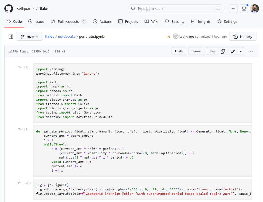
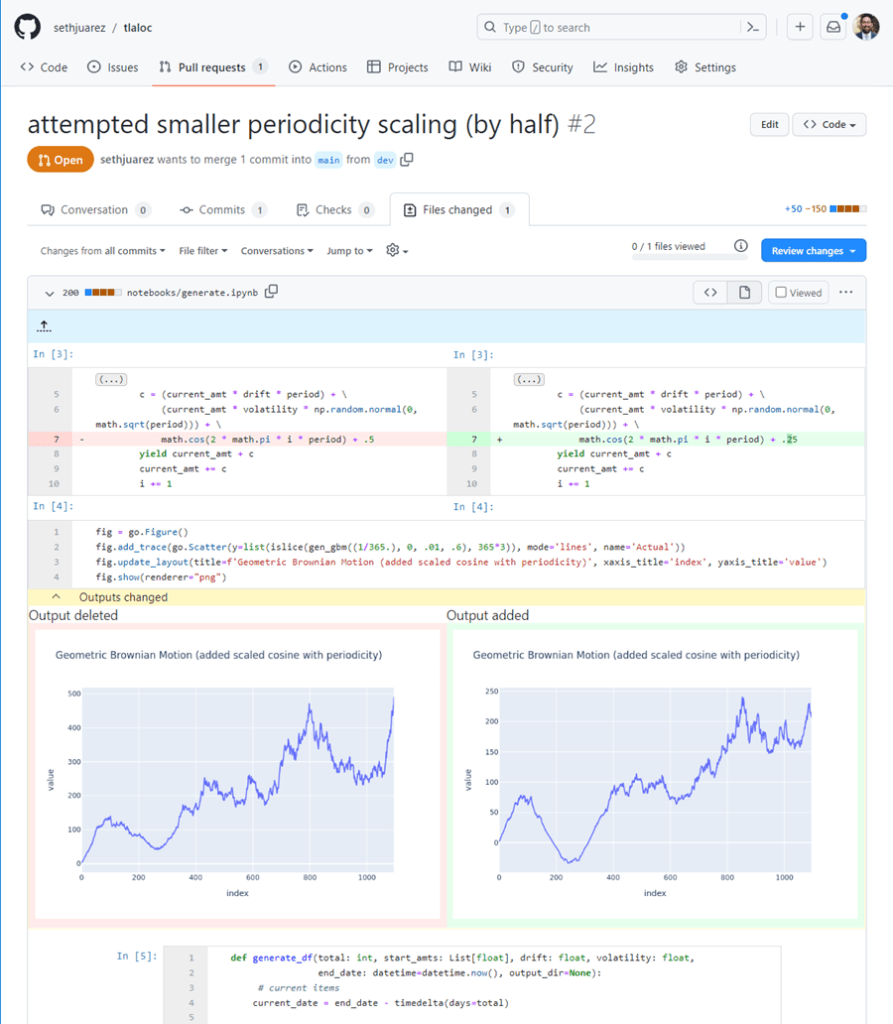
This improved rendering experience is amazing (and there’s a lovely dark mode too). In a recent pull-request I also noticed the following:
Not only can I see the cells that have been added, but I can also see side-by-side the code differences within the cells, as well as the literal outputs. I can see at a glance the code that has changed and the effect it produces thanks to NbDime running under the hood (shout out to the community for this awesome package).
Notebook Execution (and more)
While the rendering additions to GitHub are fantastic, there’s still the issue of executing the things in a reliable way when I’m away from my desk. Here’s a couple of gems we introduced at GitHub Universe to make these issues go away:
GPUs for Codespaces
Zero-config notebooks in Codespaces
Edit your notebooks from VS Code, PyCharm, JupyterLab, on the web, or even using the CLI (powered by Codespaces)
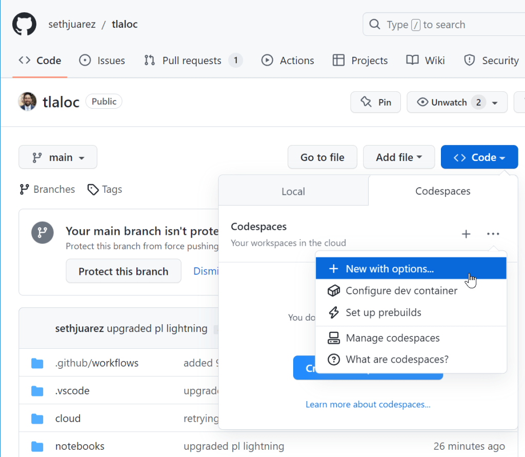
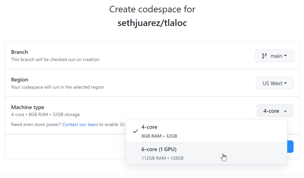
I decided to try these things out for myself by opening an existing forecasting project that uses PyTorch to do time-series analysis. I dutifully created a new Codespace (but with options since I figured I would need to tell it to use a GPU).
Sure enough, there was a nice GPU option:
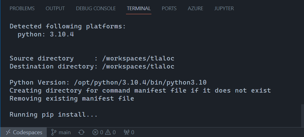
That was it! Codespaces found my requirements.txt file and went to work pip installing everything I needed.
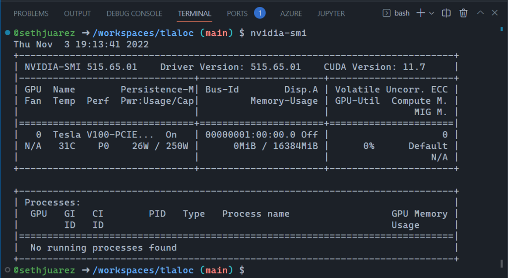
After a few minutes (PyTorch is big) I wanted to check if the GPU worked (spoiler alert below):
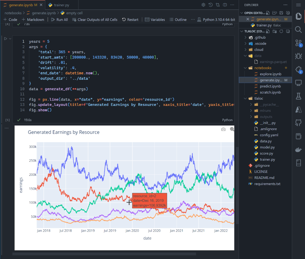
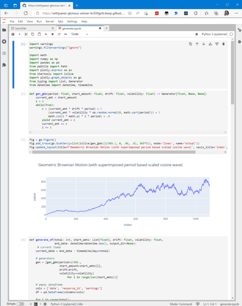
This is incredible! And, the notebook also worked exactly as it does when working locally:
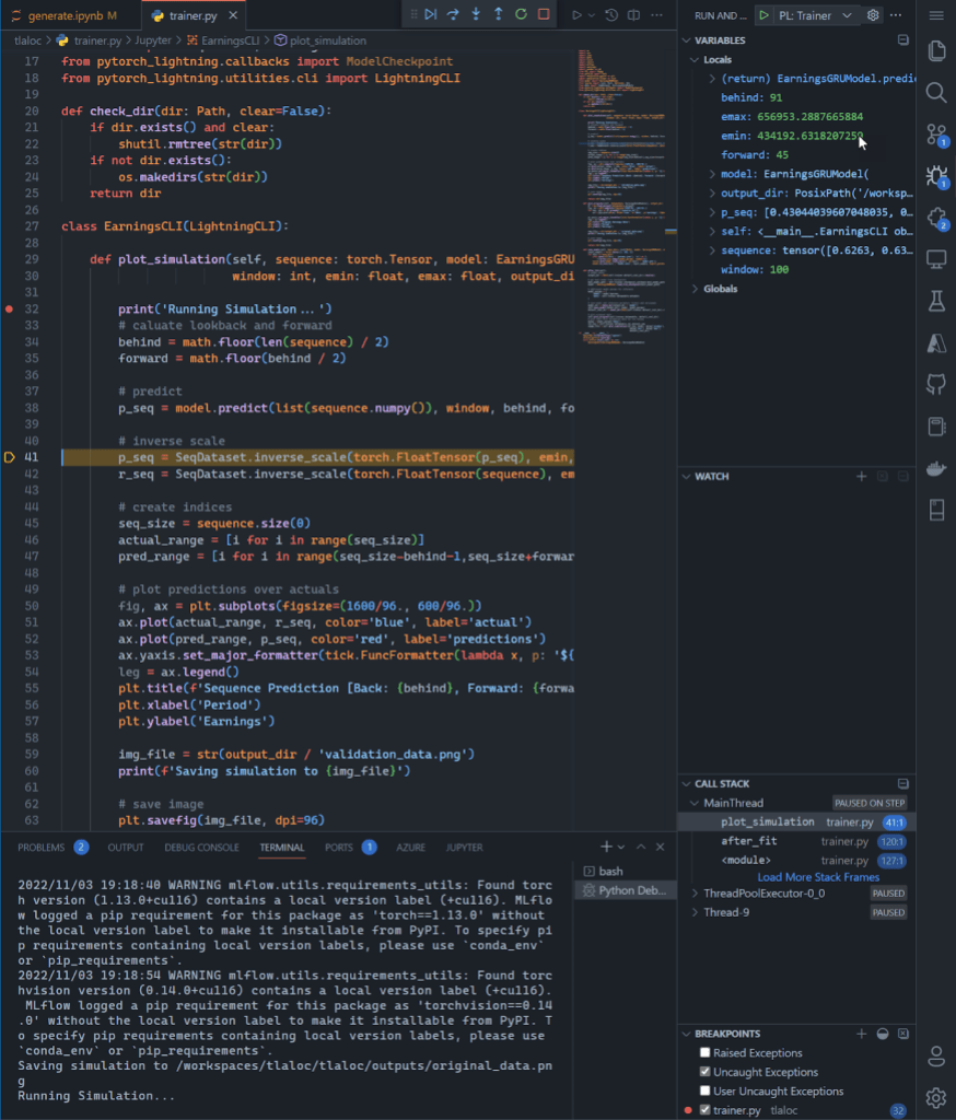
Again, this is in a browser! For kicks and giggles, I wanted to see if I could run the full blown model building process. For context, I believe notebooks are great for exploration but can become brittle when moving to repeatable processes. Eventually MLOps requires the movement of the salient code to their own scripts modules/scripts. In fact, it’s how I structure all my ML projects. If you sneak a peek above, you will see a notebooks folder and then a folder that contains the model training Python files. As an avid VSCode user I also set up a way to debug the model building process. So I crossed my fingers and started the debugging process:
I know this is a giant screenshot, but I wanted to show the full gravity of what is happening in the browser: I am debugging the build of a deep learning PyTorch model – with breakpoints and everything – on a GPU.
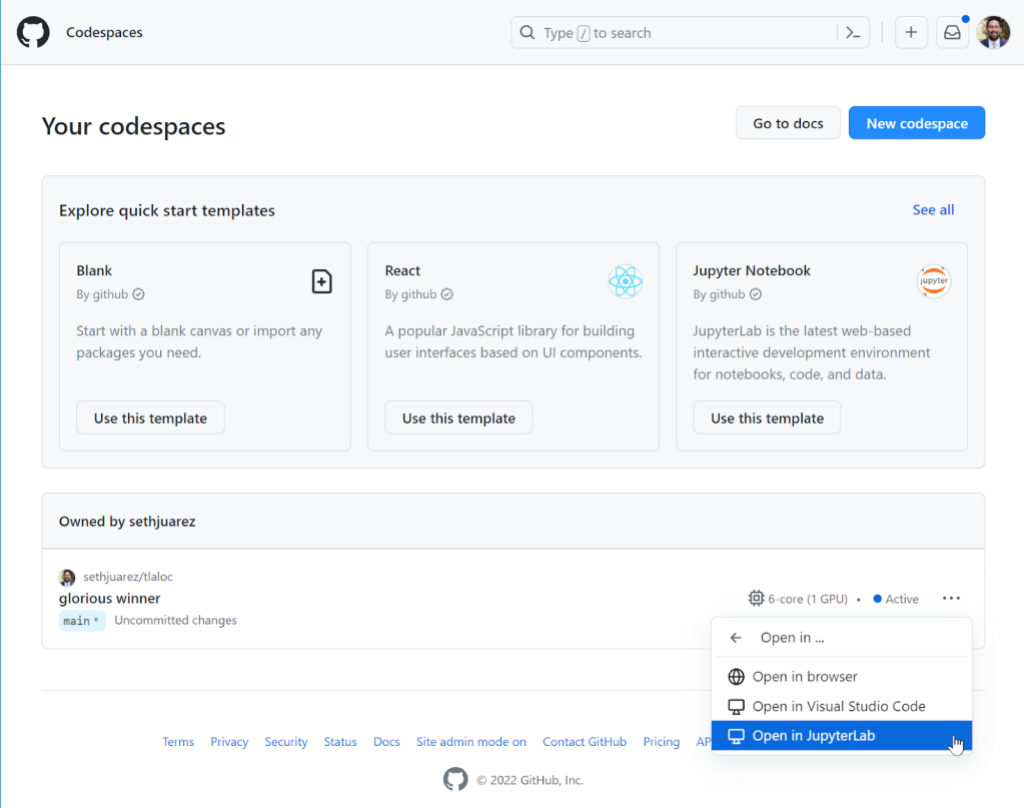
The last thing I wanted to show is the new JupyterLab feature enabled via the CLI or directly from the Codespaces page:
For some, JupyterLab is an indispensable part of their ML process – which is why it’s something we now support in its full glory:
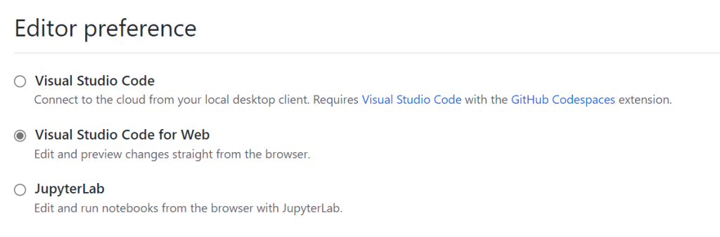
What if you’re a JupyterLab user only and don’t want to use the “Open In…” menu every time? There’s a setting for that here:
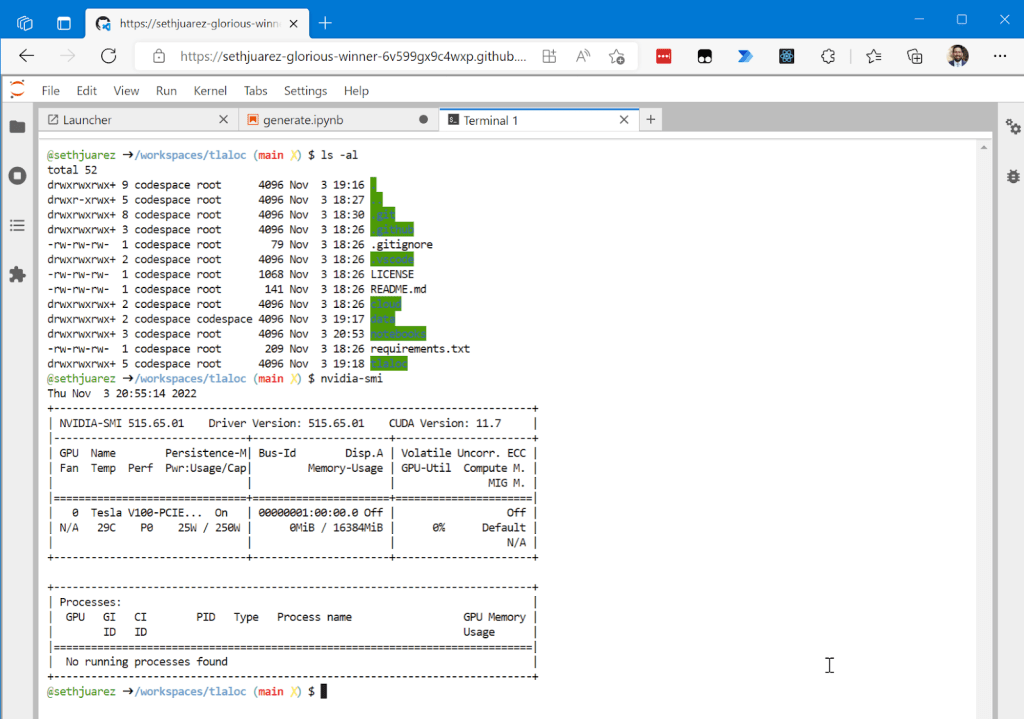
And because there’s always that one person who likes to do machine learning only from the command line (you know who I’m talking about):
For good measure I wanted to show you that given it’s the same container, the GPU is still available.
Now, what if you want to just start up a notebook and try something? A File -> New Notebook experience is also available simply using this link: https://codespace.new/jupyter.
Summary
Like I said earlier, I’m a huge fan of machine learning and GitHub. The fact that we’re adding features to make the two better together is awesome. Now this might be a coincidence (I personally don’t think so), but the container name selected by Codespaces for this little exercise sums up how this all makes me feel: sethjuarez-glorious-winner (seriously, look at container url).
Would love to hear your thoughts on these and any other features you think would make machine learning and GitHub better together. In the meantime, get ready for the upcoming GPU SKU launch by signing up to be on waitlist. Until next time!
At Netflix, part of what we do is build tools to help our creatives make exciting videos to share with the world. Today, we’d like to share some of the work we’ve been doing on match cuts.
In film, a match cut is a transition between two shots that uses similar visual framing, composition, or action to fluidly bring the viewer from one scene to the next. It is a powerful visual storytelling tool used to create a connection between two scenes.
[Spoiler alert] consider this scene from Squid Game:
The players voted to leave the game after red-light green-light, and are back in the real world. After a rough night, Gi Hung finds another calling card and considers returning to the game. As he waits for the van, a series of powerful match cuts begins, showing the other characters doing the exact same thing. We never see their stories, but because of the way it was edited, we instinctively understand that they made the same decision. This creates an emotional bond between these characters and ties them together.
A more common example is a cut from an older person to a younger person (or vice versa), usually used to signify a flashback (or flashforward). This is sometimes used to develop the story of a character. This could be done with words verbalized by a narrator or a character, but that could ruin the flow of a film, and it is not nearly as elegant as a single well executed match cut.
An example from Oldboy. A child wipes their eyes on a train, which cuts to a flashback of a younger child also wiping their eyes. We as the viewer understand that the next scene must be from this child’s upbringing.A flashforward from a young Indian Jones to an older Indian Jones conveys to the viewer that what we just saw about his childhood makes him the person he is today.
Here is one of the most famous examples from Stanley Kubrik’s 2001: A Space Odyssey. A bone is thrown into the air. As it spins, a single instantaneous cut brings the viewer from the prehistoric first act of the film into the futuristic second act. This highly artistic cut suggests that mankind’s evolution from primates to space technology is natural and inevitable.
Match cutting is also widely used outside of film. They can be found in trailers, like this sequence of shots from the trailer for Firefly Lane.
Match cutting is considered one of the most difficultvideo editing techniques, because finding a pair of shots that match can take days, if not weeks. An editor typically watches one or more long-form videos and relies on memory or manual tagging to identify shots that would match to a reference shot observed earlier.
A typical two hour movie might have around 2,000 shots, which means there are roughly 2 million pairs of shots to compare. It quickly becomes impossible to do this many comparisons manually, especially when trying to find match cuts across a 10 episode series, or multiple seasons of a show, or across multiple different shows.
What’s needed in the art of match cutting is tools to help editors find shots that match well together, which is what we’ve started building.
Our Initial Approach
Collecting training data is much more difficult compared to more common computer vision tasks. While some types of match cuts are more obvious, others are more subtle and subjective.
For instance, consider this match cut from Lawrence of Arabia. A man blows a match out, which cuts into a long, silent shot of a sunrise. It’s difficult to explain why this works, but many creatives recognize this as one of the greatest match cuts in film.
To avoid such complexities, we started with a more well-defined flavor of match cuts: ones where the visual framing of a person is aligned, aka frame matching. This came from the intuition of our video editors, who said that a large percentage of match cuts are centered around matching the silhouettes of people.
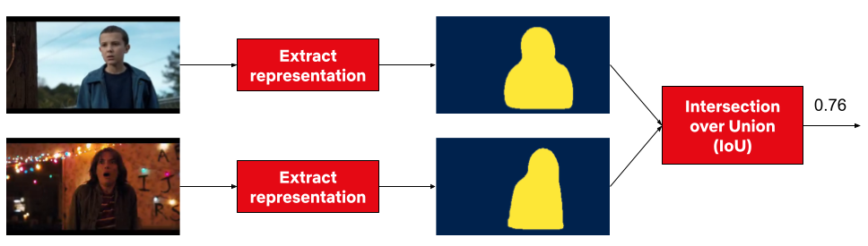
We tried several approaches, but ultimately what worked well for frame matching was instance segmentation. The output of segmentation models gives us a pixel mask of which pixels belong to which objects. We take the segmentation output of two different frames, and compute intersection over union (IoU) between the two. We then rank pairs using IoU and surface high-scoring pairs as candidates.
A few other details were added along the way. To deal with not having to brute force every single pair of frames, we only took the middle frame of each shot, since many frames look visually similar within a single shot. To deal with similar frames from different shots, we performed image deduplication upfront. In our early research, we simply discarded any mask that wasn’t a person to keep things simple. Later on, we added non-person masks back to be able to find frame match cuts of animals and objects.
A series of frame match cuts of animals from Our planet.Object frame match from Paddington 2.
Action and Motion
At this point, we decided to move onto a second flavor of match cutting: action matching. This type of match cut involves the continuation of motion of object or person A’s motion to the object or person B’s motion in another shot (A and B can be the same so long as the background, clothing, time of day, or some other attribute changes between the two shots).
To capture this type of information, we had to move beyond image level and extend into video understanding, action recognition, and motion. Optical flow is a common technique used to capture motion, so that’s what we tried first.
Consider the following shots and the corresponding optical flow representations:
A red pixel means the pixel is moving to the right. A bluepixel means the pixel is moving to the left. The intensity of the color represents the magnitude of the motion. The optical flow representations on the right show a temporal average of all the frames. While averaging can be a simple way to match the dimensionality of the data for clips of different duration, the downside is that some valuable information is lost.
When we substituted optical flow in as the shot representations (replacing instance segmentation masks) and used cosine similarity in place of IoU, we found some interesting results.
We saw that a large percentage of the top matches were actually matching based on similar camera movement. In the example above, purple in the optical flow diagram means the pixel is moving up. This wasn’t what we were expecting, but it made sense after we saw the results. For most shots, the number of background pixels outnumbers the number of foreground pixels. Therefore, it’s not hard to see why a generic similarity metric giving equal weight to each pixel would surface many shots with similar camera movement.
Here are a couple of matches found using this method:
While this wasn’t what we were initially looking for, our video editors were delighted by this output, so we decided to ship this feature as is.
Our research into true action matching still remains as future work, where we hope to leverage action recognition and foreground-background segmentation.
Match cutting system
The two flavors of match cutting we explored share a number of common components. We realized that we can break the process of finding matching pairs into five steps.
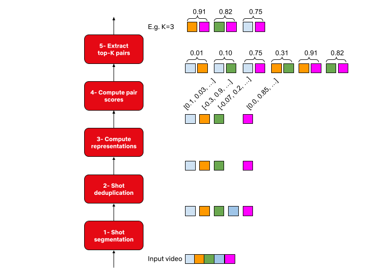
System diagram for match cutting. The input is a video file (film or series episode) and the output is K match cut candidates of the desired flavor. Each colored square represents a different shot. The original input video is broken into a sequence of shots in step 1. In Step 2, duplicate shots are removed (in this example the fourth shot is removed). In step 3, we compute a representation of each shot depending on the flavor of match cutting that we’re interested in. In step 4 we enumerate all pairs and compute a score for each pair. Finally, in step 5, we sort pairs and extract the top K (e.g. K=3 in this illustration).
1- Shot segmentation
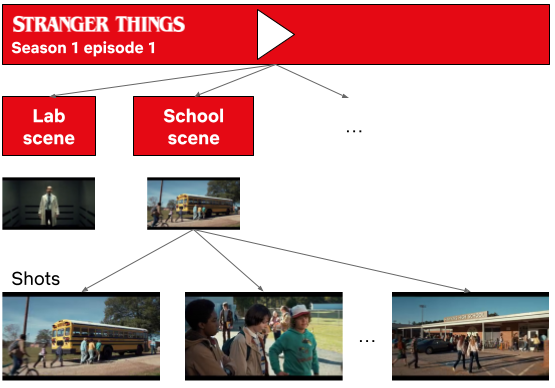
Movies, or episodes in a series, consist of a number of scenes. Scenes typically transpire in a single location and continuous time. Each scene can be one or many shots- where a shot is defined as a sequence of frames between two cuts. Shots are a very natural unit for match cutting, and our first task was to segment a movie into shots.
Stranger Things season 1 episode 1 broken down into scenes and shots.
Shots are typically a few seconds long, but can be much shorter (less than a second) or minutes long in rare cases. Detecting shot boundaries is largely a visual task and very accurate computer vision algorithms have been designed and are available. We used an in-house shot segmentation algorithm, but similar results can be achieved with open source solutions such as PySceneDetect and TransNet v2.
2- Shot deduplication
Our early attempts surfaced many near-duplicate shots. Imagine two people having a conversation in a scene. It’s common to cut back and forth as each character delivers a line.
These near-duplicate shots are not very interesting for match cutting and we quickly realized that we need to filter them out. Given a sequence of shots, we identified groups of near-duplicate shots and only retained the earliest shot from each group.
Identifying near-duplicate shots
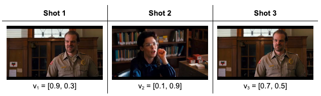
Given the following pair of shots, how do you determine if the two are near-duplicates?
You would probably inspect the two visually and look for differences in colors, presence of characters and objects, poses, and so on. We can use computer vision algorithms to mimic this approach. Given a shot, we can use an algorithm that’s been trained on a large dataset of videos (or images) and can describe it using a vector of numbers.
An encoder represents a shot from Stranger Things using a vector of numbers.
Given this algorithm (typically called an encoder in this context), we can extract a vector (aka embedding) for a pair of shots, and compute how similar they are. The vectors that such encoders produce tend to be high dimensional (hundreds or thousands of dimensions).
To build some intuition for this process, let’s look at a contrived example with 2 dimensional vectors.
Three shots from Stranger Things and the corresponding vector representations.
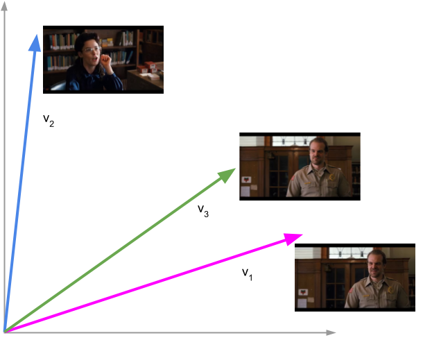
The following is a depiction of these vectors:
Shots 1 and 3 are near-duplicates. The vectors representing these shots are close to each other. All shots are from Stranger Things.
Shots 1 and 3 are near-duplicates and we see that vectors 1 and 3 are close to each other. We can quantify closeness between a pair of vectors using cosine similarity, which is a value between -1 and 1. Vectors with cosine similarity close to 1 are considered similar.
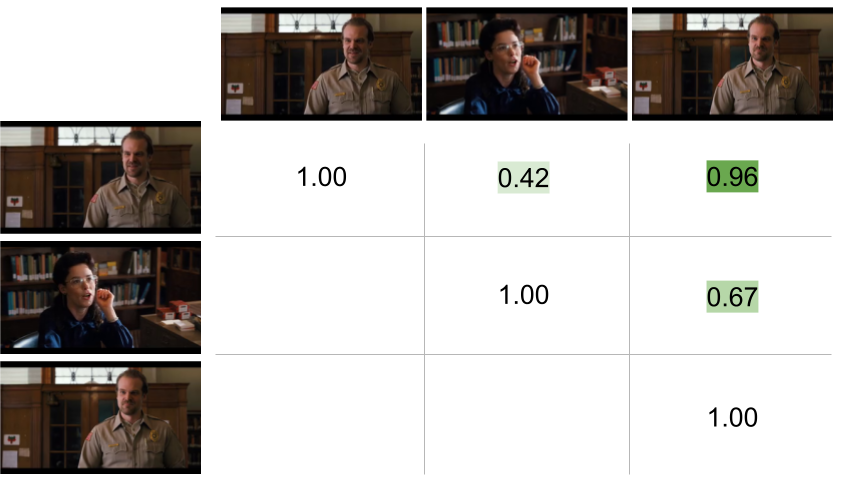
The following table shows the cosine similarity between pairs of shots:
Shots 1 and 3 have high cosine similarity (0.96) and are considered near-duplicates while shots 1 and 2 have a smaller cosine similarity value (0.42) and are not considered near-duplicates. Note that the cosine similarity of a vector with itself is 1 (i.e. it’s perfectly similar to itself) and that cosine similarity is commutative. All shots are from Stranger Things.
This approach helps us to formalize a concrete algorithmic notion of similarity.
3- Compute representations
Steps 1 and 2 are agnostic to the flavor of match cutting that we’re interested in finding. This step is meant for capturing the matching semantics that we are interested in. As we discussed earlier, for frame match cutting, this can be instance segmentation, and for camera movement, we can use optical flow.
However, there are many other possible options to represent each shot that can help us do the matching. These can be heuristically defined ahead of time based on our knowledge of the flavors, or can be learned from labeled data.
4- Compute pair scores
In this step, we compute a similarity score for all pairs. The similarity score function takes a pair of representations and produces a number. The higher this number, the more similar the pairs are deemed to be.
Steps 3 and 4 for a pair of shots from Stranger Things. In this example the representation is the person instance segmentation mask and the metric is IoU.
5- Extract top-K results
Similar to the first two steps, this step is also agnostic to the flavor. We simply rank pairs by the computed score in step 4, and take the top K (a parameter) pairs to be surfaced to our video editors.
Using this flexible abstraction, we have been able to explore many different options by picking different concrete implementations for steps 3 and 4.
Dataset
How well does this system work? To answer this question, we decided to collect a labeled dataset of approximately 20k labeled pairs. Each pair was annotated by 3 video editors. For frame match cutting, the three video editors were in perfect agreement (i.e. all three selected the same label) 84% of the time. For motion match cutting, which is a more nuanced and subjective task, perfect agreement was 75%.
We then took the majority label for each pair and used it to evaluate our model.
We started with 100 movies, which produced 128k shots and 8.2 billion unique pairs. This diagram depicts the process of reducing this set down to the final set of 19,305 pairs that were annotated.
Evaluation
Binary classification with frozen embeddings
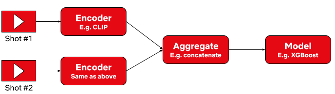
With the above dataset with binary labels, we are armed to train our first model. We extracted fixed embeddings from a variety of image, video, and audio encoders (a model or algorithm that extracts a representation given a video clip) for each pair and then aggregated the results into a single feature vector to learn a classifier on top of.
We extracted fixed embeddings using the same encoder for each shot. Then we aggregated the embeddings and passed the aggregation results to a classification model.
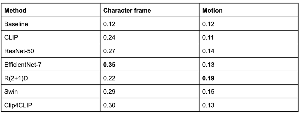
We surface top ranking pairs to video editors. A high quality match cutting system places match cuts at the top of the list by producing higher scores. We used Average Precision (AP) as our evaluation metric. AP is an information retrieval metric that is suitable for ranking scenarios such as ours. AP ranges between 0 and 1, where higher values reflect a higher quality model.
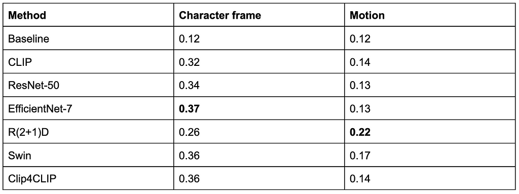
The following table summarizes our results:
Reporting AP on the test set. Baseline is a random ranking of the pairs, which for AP is equivalent to the positive prevalence of each task in expectation.
A second approach we considered was metric learning. This approach gives us transformed embeddings which can be indexed and retrieved using Approximate Nearest Neighbor (ANN) methods.
Reporting AP on the test set. Baseline is a random ranking of the pairs similar to the previous section.
Leveraging ANN, we have been able to find matches across hundreds of shows (on the order of tens of millions of shots) in seconds.
If you’re interested in more technical details make sure you take a look at our preprint paperhere.
Conclusion
There are many more ideas that have yet to be tried: other types of match cuts such as action, light, color, and sound, better representations, and end-to-end model training, just to name a few.
We’ve only scratched the surface of this work and will continue to build tools like this to empower our creatives. If this type of work interests you, we are always looking for collaboration opportunities and hiring great machine learning engineers, researchers, and interns to help build exciting tools.
We’ll leave you with this teaser for Firefly Lane, edited by Aly Parmelee, which was the first piece made with the help of the match cutting tool:
Welcome to the first post in our multi-part series on how Netflix is developing and using machine learning (ML) to help creators make better media — from TV shows to trailers to movies to promotional art and so much more.
Media is at the heart of Netflix. It’s our medium for delivering a range of emotions and experiences to our members. Through each engagement, media is how we bring our members continued joy.
This blog series will take you behind the scenes, showing you how we use the power of machine learning to create stunning media at a global scale.
At Netflix, we launch thousands of new TV shows and movies every year for our members across the globe. Each title is promoted with a custom set of artworks and video assets in support of helping each title find their audience of fans. Our goal is to empower creators with innovative tools that support them in effectively and efficiently create the best media possible.
With media-focused ML algorithms, we’ve brought science and art together to revolutionize how content is made. Here are just a few examples:
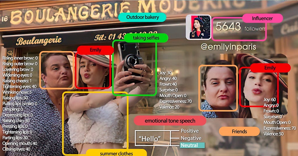
We maintain a growing suite of video understanding models that categorize characters, storylines, emotions, and cinematography. These timecode tags enable efficient discovery, freeing our creators from hours of categorizing footage so they can focus on creative decisions instead.
We arm our creators with rich insights derived from our personalization system, helping them better understand our members and gain knowledge to produce content that maximizes their joy.
We invest in novel algorithms for bringing hard-to-execute editorial techniques easily to creators’ fingertips, such as match cutting and automated rotoscoping/matting.
One of our competitive advantages is the instant feedback we get from our members and creator teams, like the success of assets for content choosing experiences and internal asset creation tools. We use these measurements to constantly refine our research, examining which algorithms and creative strategies we invest in. The feedback we collect from our members also powers our causal machine learning algorithms, providing invaluable creative insights on asset generation.
In this blog series, we will explore our media-focused ML research, development, and opportunities related to the following areas:
Computer vision: video understanding search and match cut tools
VFX and Computer graphics: matting/rotoscopy, volumetric capture to digitize actors/props/sets, animation, and relighting
Audio and Speech
Content: understanding, extraction, and knowledge graphs
Infrastructure and paradigms
We are continuously investing in the future of media-focused ML. One area we are expanding into is multimodal content understanding — a fundamental ML research that utilizes multiple sources of information or modality (e.g. video, audio, closed captions, scripts) to capture the full meaning of media content. Our teams have demonstrated value and observed success by modeling different combinations of modalities, such as video and text, video and audio, script alone, as well as video, audio and scripts together. Multimodal content understanding is expected to solve the most challenging problems in content production, VFX, promo asset creation, and personalization.
We are also using ML to transform the way we create Netflix TV shows and movies. Our filmmakers are embracing Virtual Production (filming on specialized light and MoCap stages while being able to view a virtual environment and characters). Netflix is building prototype stages and developing deep learning algorithms that will maximize cost efficiency and adoption of this transformational tech. With virtual production, we can digitize characters and sets as 3D models, estimate lighting, easily relight scenes, optimize color renditions, and replace in-camera backgrounds via semantic segmentation.
Most importantly, in close collaboration with creators, we are building human-centric approaches to creative tools, from VFX to trailer editing. Context, not control, guides the work for data scientists and algorithm engineers at Netflix. Contributors enjoy a tremendous amount of latitude to come up with experiments and new approaches, rapidly test them in production contexts, and scale the impact of their work. Our leadership in this space hinges on our reliance on each individual’s ideas and drive towards a common goal — making Netflix the home of the best content and creative experience in the world.
Working on media ML at Netflix is a unique opportunity to push the boundaries of what’s technically and creatively possible. It’s a cutting edge and quickly evolving research area. The progress we’ve made so far is just the beginning. Our goal is to research and develop machine learning and computer vision tools that put power into the hands of creators and support them in making the best media possible.
We look forward to sharing our work with you across this blog series and beyond.
If these types of challenges interest you, please let us know! We are always looking for great people who are inspired by machine learning and computer vision to join our team.
Streaming services serve content to millions of users all over the world. These services allow users to stream or download content across a broad category of devices including mobile phones, laptops, and televisions. However, some restrictions are in place, such as the number of active devices, the number of streams, and the number of downloaded titles. Many users across many platforms make for a uniquely large attack surface that includes content fraud, account fraud, and abuse of terms of service. Detection of fraud and abuse at scale and in real-time is highly challenging.
Data analysis and machine learning techniques are great candidates to help secure large-scale streaming platforms. Even though such techniques can scale security solutions proportional to the service size, they bring their own set of challenges such as requiring labeled data samples, defining effective features, and finding appropriate algorithms. In this work, by relying on the knowledge and experience of streaming security experts, we define features based on the expected streaming behavior of the users and their interactions with devices. We present a systematic overview of the unexpected streaming behaviors together with a set of model-based and data-driven anomaly detection strategies to identify them.
Background on Anomaly Detection
Anomalies (also known as outliers) are defined as certain patterns (or incidents) in a set of data samples that do not conform to an agreed-upon notion of normal behavior in a given context.
There are two main anomaly detection approaches, namely, (i) rule-based, and (ii) model-based. Rule-based anomaly detection approaches use a set of rules which rely on the knowledge and experience of domain experts. Domain experts specify the characteristics of anomalous incidents in a given context and develop a set of rule-based functions to discover the anomalous incidents. As a result of this reliance, the deployment and use of rule-based anomaly detection methods become prohibitively expensive and time-consuming at scale, and cannot be used for real-time analyses. Furthermore, the rule-based anomaly detection approaches require constant supervision by experts in order to keep the underlying set of rules up-to-date for identifying novel threats. Reliance on experts can also make rule-based approaches biased or limited in scope and efficacy.
On the other hand, in model-based anomaly detection approaches, models are built and used to detect anomalous incidents in a fairly automated manner. Although model-based anomaly detection approaches are more scalable and suitable for real-time analysis, they highly rely on the availability of (often labeled) context-specific data. Model-based anomaly detection approaches, in general, are of three kinds, namely, (i) supervised, (ii) semi-supervised, and (iii) unsupervised. Given a labeled dataset, a supervised anomaly detection model can be built to distinguish between anomalous and benign incidents. In semi-supervised anomaly detection models, only a set of benign examples are required for training. These models learn the distributions of benign samples and leverage that knowledge for identifying anomalous samples at the inference time. Unsupervised anomaly detection models do not require any labeled data samples, but it is not straightforward to reliably evaluate their efficacy.
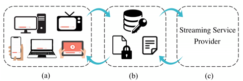
Figure 1. Schematic of a streaming service platform: (a) illustrates device types that can be used for streaming, (b) designates the set of authentication and authorization systems such as license and manifest servers for providing encrypted contents as well as decryption keys and manifests, and (c) shows the streaming service provider, as a surrogate entity for digital content providers, that interacts with the other two components.
Streaming Platforms
Commercial streaming platforms shown in Figure 1 mainly rely on Digital Rights Management (DRM) systems. DRM is a collection of access control technologies that are used for protecting the copyrights of digital media such as movies and music tracks. DRM helps the owners of digital products prevent illegal access, modification, and distribution of their copyrighted work. DRM systems provide continuous content protection against unauthorized actions on digital content and restrict it to streaming and in-time consumption. The backbone of DRM is the use of digital licenses, which specify a set of usage rights for the digital content and contain the permissions from the owner to stream the content via an on-demand streaming service.
On the client’s side, a request is sent to the streaming server to obtain the protected encrypted digital content. In order to stream the digital content, the user requests a license from the clearinghouse that verifies the user’s credentials. Once a license gets assigned to a user, using a Content Decryption Module (CDM), the protected content gets decrypted and becomes ready for preview according to the usage rights enforced by the license. A decryption key gets generated using the license, which is specific to a certain movie title, can only be used by a particular account on a given device, has a limited lifetime, and enforces a limit on how many concurrent streams are allowed.
Another relevant component that is involved in a streaming experience is the concept of manifest. Manifest is a list of video, audio, subtitles, etc. which comes in the form of a few Uniform Resource Locators (URLs) that are used by the clients to get the movie streams. Manifest is requested by the client and gets delivered to the player before the license request, and it itemizes the available streams.
Data
Data Labeling
For the task of anomaly detection in streaming platforms, as we have neither an already trained model nor any labeled data samples, we use structural a priori domain-specific rule-based assumptions, for data labeling. Accordingly, we define a set of rule-based heuristics used for identifying anomalous streaming behaviors of clients and label them as anomalous or benign. The fraud categories that we consider in this work are (i) content fraud, (ii) service fraud, and (iii) account fraud. With the help of security experts, we have designed and developed heuristic functions in order to discover a wide range of suspicious behaviors. We then use such heuristic functions for automatically labeling the data samples. In order to label a set of benign (non-anomalous) accounts a group of vetted users that are highly trusted to be free of any forms of fraud is used.
Next, we share three examples as a subset of our in-house heuristics that we have used for tagging anomalous accounts:
(i) Rapid license acquisition: a heuristic that is based on the fact that benign users usually watch one content at a time and it takes a while for them to move on to another content resulting in a relatively low rate of license acquisition. Based on this reasoning, we tag all the accounts that acquire licenses very quickly as anomalous.
(ii) Too many failed attempts at streaming: a heuristic that relies on the fact that most devices stream without errors while a device, in trial and error mode, in order to find the “right’’ parameters leaves a long trail of errors behind. Abnormally high levels of errors are an indicator of a fraud attempt.
(iii) Unusual combinations of device types and DRMs: a heuristic that is based on the fact that a device type (e.g., a browser) is normally matched with a certain DRM system (e.g., Widevine). Unusual combinations could be a sign of compromised devices that attempt to bypass security enforcements.
It should be noted that the heuristics, even though work as a great proxy to embed the knowledge of security experts in tagging anomalous accounts, may not be completely accurate and they might wrongly tag accounts as anomalous (i.e., false-positive incidents), for example in the case of a buggy client or device. That’s up to the machine learning model to discover and avoid such false-positive incidents.
Data Featurization
A complete list of features used in this work is presented in Table 1. The features mainly belong to two distinct classes. One class accounts for the number of distinct occurrences of a certain parameter/activity/usage in a day. For instance, the dist_title_cnt feature characterizes the number of distinct movie titles streamed by an account. The second class of features on the other hand captures the percentage of a certain parameter/activity/usage in a day.
Due to confidentiality reasons, we have partially obfuscated the features, for instance, dev_type_a_pct, drm_type_a_pct, and end_frmt_a_pct are intentionally obfuscated and we do not explicitly mention devices, DRM types, and encoding formats.
Table 1. The list of streaming related features with the suffixes pct and cnt respectively referring to percentage and count
Data Statistics
In this part, we present the statistics of the features presented in Table 1. Over 30 days, we have gathered 1,030,005 benign and 28,045 anomalous accounts. The anomalous accounts have been identified (labeled) using the heuristic-aware approach. Figure 2(a) shows the number of anomalous samples as a function of fraud categories with 8,741 (31%), 13,299 (47%), 6,005 (21%) data samples being tagged as content fraud, service fraud, and account fraud, respectively. Figure 2(b) shows that out of 28,045 data samples being tagged as anomalous by the heuristic functions, 23,838 (85%), 3,365 (12%), and 842 (3%) are respectively considered as incidents of one, two, and three fraud categories.
Figure 3 presents the correlation matrix of the 23 data features described in Table 1 for clean and anomalous data samples. As we can see in Figure 3 there are positive correlations between features that correspond to device signatures, e.g., dist_cdm_cnt and dist_dev_id_cnt, and between features that refer to title acquisition activities, e.g., dist_title_cnt and license_cnt.
Figure 2. Number of anomalous samples as a function of (a) fraud categories and (b) number of tagged categories.Figure 3. Correlation matrix of the features presented in Table 1 for (a) clean and (b) anomalous data samples.
Label Imbalance Treatment
It is well known that class imbalance can compromise the accuracy and robustness of the classification models. Accordingly, in this work, we use the Synthetic Minority Over-sampling Technique (SMOTE) to over-sample the minority classes by creating a set of synthetic samples.
Figure 4 shows a high-level schematic of Synthetic Minority Over-sampling Technique (SMOTE) with two classes shown in green and red where the red class has fewer number of samples present, i.e., is the minority class, and gets synthetically upsampled.
For evaluating the performance of the anomaly detection models we consider a set of evaluation metrics and report their values. For the one-class as well as binary anomaly detection task, such metrics are accuracy, precision, recall, f0.5, f1, and f2 scores, and area under the curve of the receiver operating characteristic (ROC AUC). For the multi-class multi-label task we consider accuracy, precision, recall, f0.5, f1, and f2 scores together with a set of additional metrics, namely, exact match ratio (EMR) score, Hamming loss, and Hamming score.
Model Based Anomaly Detection
In this section, we briefly describe the modeling approaches that are used in this work for anomaly detection. We consider two model-based anomaly detection approaches, namely, (i) semi-supervised, and (ii) supervised as presented in Figure 5.
The key point about the semi-supervised model is that at the training step the model is supposed to learn the distribution of the benign data samples so that at the inference time it would be able to distinguish between the benign samples (that has been trained on) and the anomalous samples (that has not observed). Then at the inference stage, the anomalous samples would simply be those that fall out of the distribution of the benign samples. The performance of One-Class methods could become sub-optimal when dealing with complex and high-dimensional datasets. However, supported by the literature, deep neural autoencoders can perform better than One-Class methods on complex and high-dimensional anomaly detection tasks.
As the One-Class anomaly detection approaches, in addition to a deep auto-encoder, we use the One-Class SVM, Isolation Forest, Elliptic Envelope, and Local Outlier Factor approaches.
Supervised Anomaly Detection
Binary Classification: In the anomaly detection task using binary classification, we only consider two classes of samples namely benign and anomalous and we do not make distinctions between the types of the anomalous samples, i.e., the three fraud categories. For the binary classification task we use multiple supervised classification approaches, namely, (i) Support Vector Classification (SVC), (ii) K-Nearest Neighbors classification, (iii) Decision Tree classification, (iv) Random Forest classification, (v) Gradient Boosting, (vi) AdaBoost, (vii) Nearest Centroid classification (viii) Quadratic Discriminant Analysis (QDA) classification (ix) Gaussian Naive Bayes classification (x) Gaussian Process Classifier (xi) Label Propagation classification (xii) XGBoost. Finally, upon doing stratified k-fold cross-validation, we carry out an efficient grid search to tune the hyper-parameters in each of the aforementioned models for the binary classification task and only report the performance metrics for the optimally tuned hyper-parameters.
Multi-Class Multi-Label Classification: In the anomaly detection task using multi-class multi-label classification, we consider the three fraud categories as the possible anomalous classes (hence multi-class), and each data sample is assigned one or more than one of the fraud categories as its set of labels (hence multi-label) using the heuristic-aware data labeling strategy presented earlier. For the multi-class multi-label classification task we use multiple supervised classification techniques, namely, (i) K-Nearest Neighbors, (ii) Decision Tree, (iii) Extra Trees, (iv) Random Forest, and (v) XGBoost.
Results and Discussion
Table 2 shows the values of the evaluation metrics for the semi-supervised anomaly detection methods. As we see from Table 2, the deep auto-encoder model performs the best among the semi-supervised anomaly detection approaches with an accuracy of around 96% and f1 score of 94%. Figure 6(a) shows the distribution of the Mean Squared Error (MSE) values for the anomalous and benign samples at the inference stage.
Table 2. The values of the evaluation metrics for a set of semi-supervised anomaly detection models.Figure 6. For the deep auto-encoder model: (a) distribution of the Mean Squared Error (MSE) values for anomalous and benign samples at the inference stage — (b) confusion matrix across benign and anomalous samples- (c) Mean Squared Error (MSE) values averaged across the anomalous and benign samples for each of the 23 features.Table 3. The values of the evaluation metrics for a set of supervised binary anomaly detection classifiers.Table 4. The values of the evaluation metrics for a set of supervised multi-class multi-label anomaly detection approaches. The values in parenthesis refer to the performance of the models trained on the original (not upsampled) dataset.
Table 3 shows the values of the evaluation metrics for a set of supervised binary anomaly detection models. Table 4 shows the values of the evaluation metrics for a set of supervised multi-class multi-label anomaly detection models.
In Figure 7(a), for the content fraud category, the three most important features are the count of distinct encoding formats (dist_enc_frmt_cnt), the count of distinct devices (dist_dev_id_cnt), and the count of distinct DRMs (dist_drm_cnt). This implies that for content fraud the uses of multiple devices, as well as encoding formats, stand out from the other features. For the service fraud category in Figure 7(b) we see that the three most important features are the count of content licenses associated with an account (license_cnt), the count of distinct devices (dist_dev_id_cnt), and the percentage use of type (a) devices by an account (dev_type_a_pct). This shows that in the service fraud category the counts of content licenses and distinct devices of type (a) stand out from the other features. Finally, for the account fraud category in Figure 7(c), we see that the count of distinct devices (dist_dev_id_cnt) dominantly stands out from the other features.
Figure 7. The normalized feature importance values (NFIV) for the multi-class multi-label anomaly detection task using the XGBoost approach in Table 4 across the three anomaly classes, i.e., (a) content fraud, (b) service fraud, and (c) account fraud.
You can find more technical details in our paper here.
Are you interested in solving challenging problems at the intersection of machine learning and security? We are always looking for great people to join us.
On November 11th 2022, Rapid7 will for the first time publish and present state-of-the-art machine learning (ML) research at AISec, the leading venue for AI/ML cybersecurity innovations. Led by Dr. Stuart Millar, Senior Data Scientist, Rapid7’s multi-disciplinary ML group has designed a novel deep learning model to automatically prioritize application security vulnerabilities and reduce false positive friction. Partnering with The Centre for Secure Information Technologies (CSIT) at Queen’s University Belfast, this is the first deep learning system to optimize DAST vulnerability triage in application security. CSIT is the UK’s Innovation and Knowledge Centre for cybersecurity, recognised by GCHQ and EPSRC as a Centre of Excellence for cybersecurity research.
Security teams struggle tremendously with prioritizing risk and managing a high level of false positive alerts, while the rise of the cloud post-Covid means web application security is more crucial than ever. Web attacks continue to be the most common type of compromise; however, high levels of false positives generated by vulnerability scanners have become an industry-wide challenge. To combat this, Rapid7’s innovative ML architecture optimizes vulnerability triage by utilizing the structure of traffic exchanges between a DAST scanner and a given web application. Leveraging convolutional neural networks and natural language processing, we designed a deep learning system that encapsulates internal representations of request and response HTTP traffic before fusing them together to make a prediction of a verified vulnerability or a false positive. This system learns from historical triage carried out by our industry-leading SMEs in Rapid7’s Managed Services division.
Given the skillset, time, and cognitive effort required to review high volumes of DAST results by hand, the addition of this deep learning capability to a scanner creates a hybrid system that enables application security analysts to rank scan results, deprioritise false positives, and concentrate on likely real vulnerabilities. With the system able to make hundreds of predictions per second, productivity is improved and remediation time reduced, resulting in stronger customer security postures. A rigorous evaluation of this machine learning architecture across multiple customers shows that 96% of false positives on average can automatically be detected and filtered out.
Rapid7’s deep learning model uses convolutional neural networks and natural language processing to represent the structure of client-server web traffic. Neither the model nor the scanner require source code access — with this hybrid approach first finding potential vulnerabilities using a scan engine, followed by the model predicting those findings as real vulnerabilities or false positives. The resultant solution enables the augmentation of triage decisions by deprioritizing false positives. These time savings are essential to reduce exposure and harden security postures — considering the average time to detect a web breach can be several months, the sooner a vulnerability can be discovered, verified and remediated, the smaller the window of opportunity for an attacker.
Now recognized as state-of-the-art research after expert peer review, Rapid7 will introduce the work at AISec on Nov 11th 2022 at the Omni Los Angeles Hotel at California Plaza. Watch this space for further developments, and download a copy of the pre-print publication here.
Machine learning security is extraordinarily difficult because the attacks are so varied—and it seems that each new one is weirder than the next. Here’s the latest: a training-time attack that forces the model to exhibit a point of view: Spinning Language Models: Risks of Propaganda-As-A-Service and Countermeasures.”
Abstract: We investigate a new threat to neural sequence-to-sequence (seq2seq) models: training-time attacks that cause models to “spin” their outputs so as to support an adversary-chosen sentiment or point of view—but only when the input contains adversary-chosen trigger words. For example, a spinned summarization model outputs positive summaries of any text that mentions the name of some individual or organization.
Model spinning introduces a “meta-backdoor” into a model. Whereas conventional backdoors cause models to produce incorrect outputs on inputs with the trigger, outputs of spinned models preserve context and maintain standard accuracy metrics, yet also satisfy a meta-task chosen by the adversary.
Model spinning enables propaganda-as-a-service, where propaganda is defined as biased speech. An adversary can create customized language models that produce desired spins for chosen triggers, then deploy these models to generate disinformation (a platform attack), or else inject them into ML training pipelines (a supply-chain attack), transferring malicious functionality to downstream models trained by victims.
To demonstrate the feasibility of model spinning, we develop a new backdooring technique. It stacks an adversarial meta-task onto a seq2seq model, backpropagates the desired meta-task output to points in the word-embedding space we call “pseudo-words,” and uses pseudo-words to shift the entire output distribution of the seq2seq model. We evaluate this attack on language generation, summarization, and translation models with different triggers and meta-tasks such as sentiment, toxicity, and entailment. Spinned models largely maintain their accuracy metrics (ROUGE and BLEU) while shifting their outputs to satisfy the adversary’s meta-task. We also show that, in the case of a supply-chain attack, the spin functionality transfers to downstream models.
This new attack dovetails with something I’ve been worried about for a while, something Latanya Sweeney has dubbed “persona bots.” This is what I wrote in my upcoming book (to be published in February):
One example of an extension of this technology is the “persona bot,” an AI posing as an individual on social media and other online groups. Persona bots have histories, personalities, and communication styles. They don’t constantly spew propaganda. They hang out in various interest groups: gardening, knitting, model railroading, whatever. They act as normal members of those communities, posting and commenting and discussing. Systems like GPT-3 will make it easy for those AIs to mine previous conversations and related Internet content and to appear knowledgeable. Then, once in a while, the AI might post something relevant to a political issue, maybe an article about a healthcare worker having an allergic reaction to the COVID-19 vaccine, with worried commentary. Or maybe it might offer its developer’s opinions about a recent election, or racial justice, or any other polarizing subject. One persona bot can’t move public opinion, but what if there were thousands of them? Millions?
These are chatbots on a very small scale. They would participate in small forums around the Internet: hobbyist groups, book groups, whatever. In general they would behave normally, participating in discussions like a person does. But occasionally they would say something partisan or political, depending on the desires of their owners. Because they’re all unique and only occasional, it would be hard for existing bot detection techniques to find them. And because they can be replicated by the millions across social media, they could have a greater effect. They would affect what we think, and—just as importantly—what we think others think. What we will see as robust political discussions would be persona bots arguing with other persona bots.
Attacks like these add another wrinkle to that sort of scenario.
At Netflix, Data and Machine Learning (ML) pipelines are widely used and have become central for the business, representing diverse use cases that go beyond recommendations, predictions and data transformations. A large number of batch workflows run daily to serve various business needs. These include ETL pipelines, ML model training workflows, batch jobs, etc. As Big data and ML became more prevalent and impactful, the scalability, reliability, and usability of the orchestrating ecosystem have increasingly become more important for our data scientists and the company.
In this blog post, we introduce and share learnings on Maestro, a workflow orchestrator that can schedule and manage workflows at a massive scale.
Motivation
Scalability and usability are essential to enable large-scale workflows and support a wide range of use cases. Our existing orchestrator (Meson) has worked well for several years. It schedules around 70 thousands of workflows and half a million jobs per day. Due to its popularity, the number of workflows managed by the system has grown exponentially. We started seeing signs of scale issues, like:
Slowness during peak traffic moments like 12 AM UTC, leading to increased operational burden. The scheduler on-call has to closely monitor the system during non-business hours.
Meson was based on a single leader architecture with high availability. As the usage increased, we had to vertically scale the system to keep up and were approaching AWS instance type limits.
With the high growth of workflows in the past few years — increasing at > 100% a year, the need for a scalable data workflow orchestrator has become paramount for Netflix’s business needs. After perusing the current landscape of workflow orchestrators, we decided to develop a next generation system that can scale horizontally to spread the jobs across the cluster consisting of 100’s of nodes. It addresses the key challenges we face with Meson and achieves operational excellence.
Challenges in Workflow Orchestration
Scalability
The orchestrator has to schedule hundreds of thousands of workflows, millions of jobs every day and operate with a strict SLO of less than 1 minute of scheduler introduced delay even when there are spikes in the traffic. At Netflix, the peak traffic load can be a few orders of magnitude higher than the average load. For example, a lot of our workflows are run around midnight UTC. Hence, the system has to withstand bursts in traffic while still maintaining the SLO requirements. Additionally, we would like to have a single scheduler cluster to manage most of user workflows for operational and usability reasons.
Another dimension of scalability to consider is the size of the workflow. In the data domain, it is common to have a super large number of jobs within a single workflow. For example, a workflow to backfill hourly data for the past five years can lead to 43800 jobs (24 * 365 * 5), each of which processes data for an hour. Similarly, ML model training workflows usually consist of tens of thousands of training jobs within a single workflow. Those large-scale workflows might create hotspots and overwhelm the orchestrator and downstream systems. Therefore, the orchestrator has to manage a workflow consisting of hundreds of thousands of jobs in a performant way, which is also quite challenging.
Usability
Netflix is a data-driven company, where key decisions are driven by data insights, from the pixel color used on the landing page to the renewal of a TV-series. Data scientists, engineers, non-engineers, and even content producers all run their data pipelines to get the necessary insights. Given the diverse backgrounds, usability is a cornerstone of a successful orchestrator at Netflix.
We would like our users to focus on their business logic and let the orchestrator solve cross-cutting concerns like scheduling, processing, error handling, security etc. It needs to provide different grains of abstractions for solving similar problems, high-level to cater to non-engineers and low-level for engineers to solve their specific problems. It should also provide all the knobs for configuring their workflows to suit their needs. In addition, it is critical for the system to be debuggable and surface all the errors for users to troubleshoot, as they improve the UX and reduce the operational burden.
Providing abstractions for the users is also needed to save valuable time on creating workflows and jobs. We want users to rely on shared templates and reuse their workflow definitions across their team, saving time and effort on creating the same functionality. Using job templates across the company also helps with upgrades and fixes: when the change is made in a template it’s automatically updated for all workflows that use it.
However, usability is challenging as it is often opinionated. Different users have different preferences and might ask for different features. Sometimes, the users might ask for the opposite features or ask for some niche cases, which might not necessarily be useful for a broader audience.
Introducing Maestro
Maestro is the next generation Data Workflow Orchestration platform to meet the current and future needs of Netflix. It is a general-purpose workflow orchestrator that provides a fully managed workflow-as-a-service (WAAS) to the data platform at Netflix. It serves thousands of users, including data scientists, data engineers, machine learning engineers, software engineers, content producers, and business analysts, for various use cases.
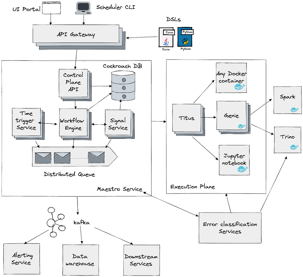
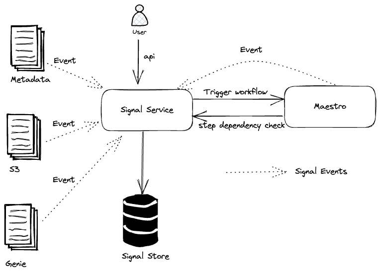
Maestro is highly scalable and extensible to support existing and new use cases and offers enhanced usability to end users. Figure 1 shows the high-level architecture.
Figure 1. Maestro high level architecture
In Maestro, a workflow is a DAG (Directed acyclic graph) of individual units of job definition called Steps. Steps can have dependencies, triggers, workflow parameters, metadata, step parameters, configurations, and branches (conditional or unconditional). In this blog, we use step and job interchangeably. A workflow instance is an execution of a workflow, similarly, an execution of a step is called a step instance. Instance data include the evaluated parameters and other information collected at runtime to provide different kinds of execution insights. The system consists of 3 main micro services which we will expand upon in the following sections.
Maestro ensures the business logic is run in isolation. Maestro launches a unit of work (a.k.a. Steps) in a container and ensures the container is launched with the users/applications identity. Launching with identity ensures the work is launched on-behalf-of the user/application, the identity is later used by the downstream systems to validate if an operation is allowed or not, for an example user/application identity is checked by the data warehouse to validate if a table read/write is allowed or not.
Workflow Engine
Workflow engine is the core component, which manages workflow definitions, the lifecycle of workflow instances, and step instances. It provides rich features to support:
Any valid DAG patterns
Popular data flow constructs like sub workflow, foreach, conditional branching etc.
Multiple failure modes to handle step failures with different error retry policies
Flexible concurrency control to throttle the number of executions at workflow/step level
Step templates for common job patterns like running a Spark query or moving data to Google sheets
Support parameter code injection using customized expression language
Workflow definition and ownership management. Timeline including all state changes and related debug info.
We use Netflix open source project Conductor as a library to manage the workflow state machine in Maestro. It ensures to enqueue and dequeue each step defined in a workflow with at least once guarantee.
Time-Based Scheduling Service
Time-based scheduling service starts new workflow instances at the scheduled time specified in workflow definitions. Users can define the schedule using cron expression or using periodic schedule templates like hourly, weekly etc;. This service is lightweight and provides an at-least-once scheduling guarantee. Maestro engine service will deduplicate the triggering requests to achieve an exact-once guarantee when scheduling workflows.
Time-based triggering is popular due to its simplicity and ease of management. But sometimes, it is not efficient. For example, the daily workflow should process the data when the data partition is ready, not always at midnight. Therefore, on top of manual and time-based triggering, we also provide event-driven triggering.
Signal Service
Maestro supports event-driven triggering over signals, which are pieces of messages carrying information such as parameter values. Signal triggering is efficient and accurate because we don’t waste resources checking if the workflow is ready to run, instead we only execute the workflow when a condition is met.
Signals are used in two ways:
A trigger to start new workflow instances
A gating function to conditionally start a step (e.g., data partition readiness)
Signal service goals are to
Collect and index signals
Register and handle workflow trigger subscriptions
Register and handle the step gating functions
Captures the lineage of workflows triggers and steps unblocked by a signal
Figure 2. Signal service high level architecture
The maestro signal service consumes all the signals from different sources, e.g. all the warehouse table updates, S3 events, a workflow releasing a signal, and then generates the corresponding triggers by correlating a signal with its subscribed workflows. In addition to the transformation between external signals and workflow triggers, this service is also responsible for step dependencies by looking up the received signals in the history. Like the scheduling service, the signal service together with Maestro engine achieves exactly-once triggering guarantees.
Signal service also provides the signal lineage, which is useful in many cases. For example, a table updated by a workflow could lead to a chain of downstream workflow executions. Most of the time the workflows are owned by different teams, the signal lineage helps the upstream and downstream workflow owners to see who depends on whom.
Orchestration at Scale
All services in the Maestro system are stateless and can be horizontally scaled out. All the requests are processed via distributed queues for message passing. By having a shared nothing architecture, Maestro can horizontally scale to manage the states of millions of workflow and step instances at the same time.
CockroachDB is used for persisting workflow definitions and instance state. We chose CockroachDB as it is an open-source distributed SQL database that provides strong consistency guarantees that can be scaled horizontally without much operational overhead.
It is hard to support super large workflows in general. For example, a workflow definition can explicitly define a DAG consisting of millions of nodes. With that number of nodes in a DAG, UI cannot render it well. We have to enforce some constraints and support valid use cases consisting of hundreds of thousands (or even millions) of step instances in a workflow instance.
Based on our findings and user feedback, we found that in practice
Users don’t want to manually write the definitions for thousands of steps in a single workflow definition, which is hard to manage and navigate over UI. When such a use case exists, it is always feasible to decompose the workflow into smaller sub workflows.
Users expect to repeatedly run a certain part of DAG hundreds of thousands (or even millions) times with different parameter settings in a given workflow instance. So at runtime, a workflow instance might include millions of step instances.
Therefore, we enforce a workflow DAG size limit (e.g. 1K) and we provide a foreach pattern that allows users to define a sub DAG within a foreach block and iterate the sub DAG with a larger limit (e.g. 100K). Note that foreach can be nested by another foreach. So users can run millions or billions of steps in a single workflow instance.
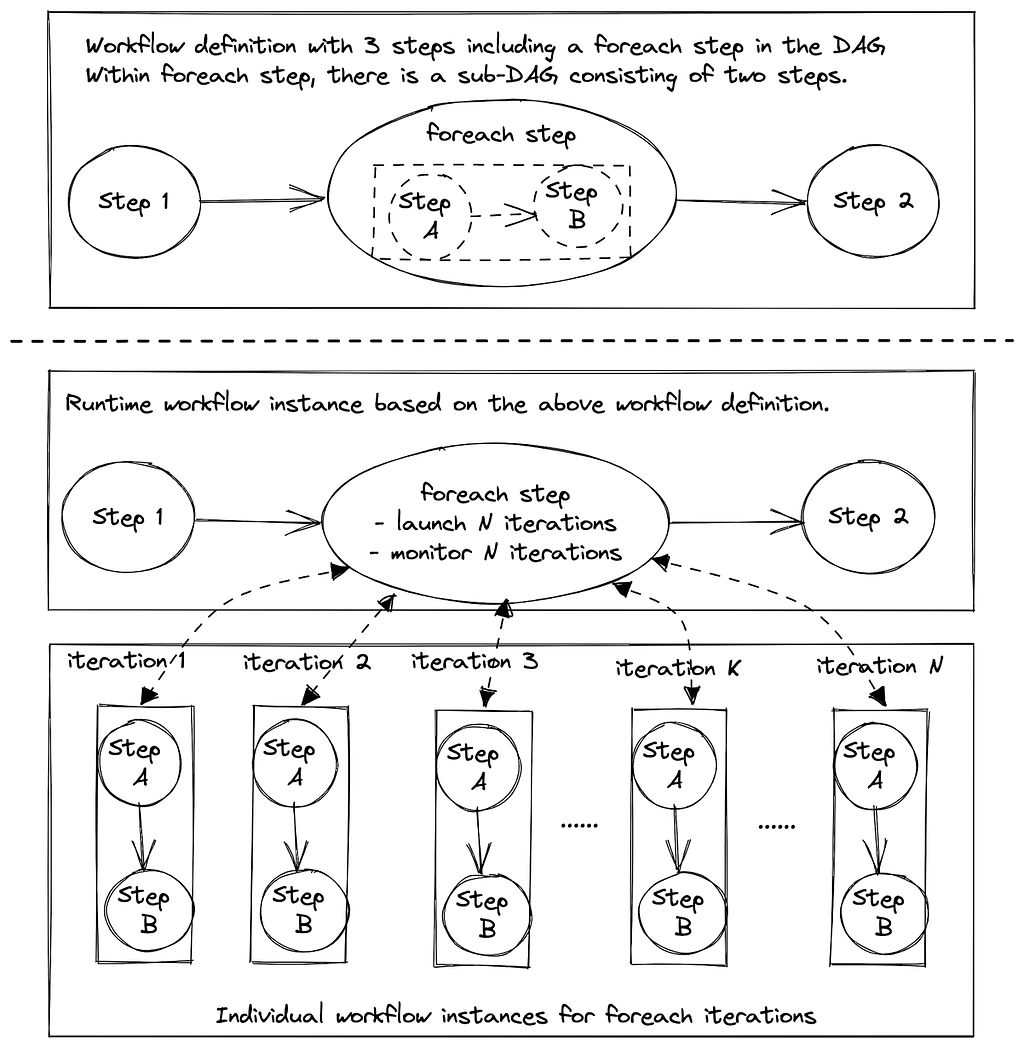
In Maestro, foreach itself is a step in the original workflow definition. Foreach is internally treated as another workflow which scales similarly as any other Maestro workflow based on the number of step executions in the foreach loop. The execution of sub DAG within foreach will be delegated to a separate workflow instance. Foreach step will then monitor and collect status of those foreach workflow instances, each of which manages the execution of one iteration.
Figure 3. Maestro’s scalable foreach design to support super large iterations
With this design, foreach pattern supports sequential loop and nested loop with high scalability. It is easy to manage and troubleshoot as users can see the overall loop status at the foreach step or view each iteration separately.
Workflow Platform for Everyone
We aim to make Maestro user friendly and easy to learn for users with different backgrounds. We made some assumptions about user proficiency in programming languages and they can bring their business logic in multiple ways, including but not limited to, a bash script, a Jupyter notebook, a Java jar, a docker image, a SQL statement, or a few clicks in the UI using parameterized workflow templates.
User Interfaces
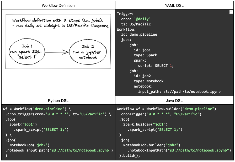
Maestro provides multiple domain specific languages (DSLs) including YAML, Python, and Java, for end users to define their workflows, which are decoupled from their business logic. Users can also directly talk to Maestro API to create workflows using the JSON data model. We found that human readable DSL is popular and plays an important role to support different use cases. YAML DSL is the most popular one due to its simplicity and readability.
Here is an example workflow defined by different DSLs.
Figure 4. An example workflow defined by YAML, Python, and Java DSLs
Additionally, users can also generate certain types of workflows on UI or use other libraries, e.g.
In Notebook UI, users can directly schedule to run the chosen notebook periodically.
In Maestro UI, users can directly schedule to move data from one source (e.g. a data table or a spreadsheet) to another periodically.
Users can use Metaflow library to create workflows in Maestro to execute DAGs consisting of arbitrary Python code.
Parameterized Workflows
Lots of times, users want to define a dynamic workflow to adapt to different scenarios. Based on our experiences, a completely dynamic workflow is less favorable and hard to maintain and troubleshooting. Instead, Maestro provides three features to assist users to define a parameterized workflow
Conditional branching
Sub-workflow
Output parameters
Instead of dynamically changing the workflow DAG at runtime, users can define those changes as sub workflows and then invoke the appropriate sub workflow at runtime because the sub workflow id is a parameter, which is evaluated at runtime. Additionally, using the output parameter, users can produce different results from the upstream job step and then iterate through those within the foreach, pass it to the sub workflow, or use it in the downstream steps.
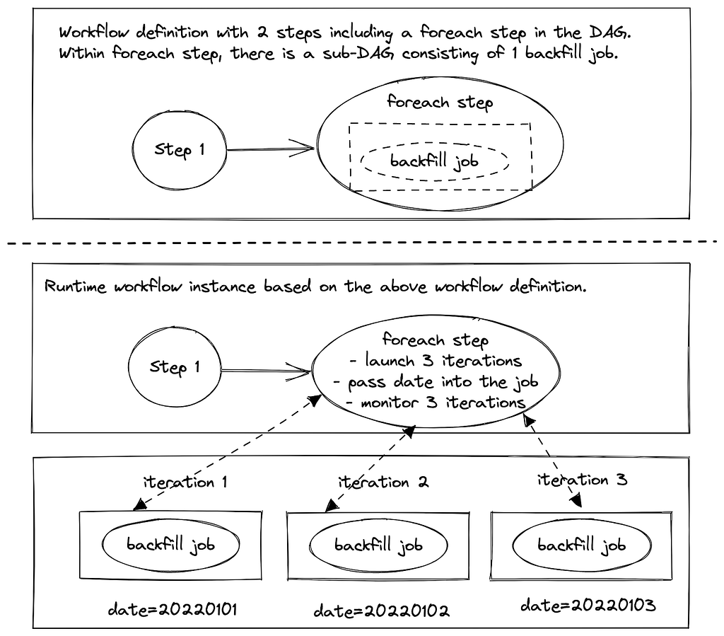
Here is an example (using YAML DSL) of backfill workflow with 2 steps. In step1, the step computes the backfill ranges and returns the dates back. Next, foreach step uses the dates from step1 to create foreach iterations. Finally, each of the backfill jobs gets the date from the foreach and backfills the data based on the date.
Figure 5. An example of using parameterized workflow for backfill data
The parameter system in Maestro is completely dynamic with code injection support. Users can write the code in Java syntax as the parameter definition. We developed our own secured expression language (SEL) to ensure security. It only exposes limited functionality and includes additional checks (e.g. the number of iteration in the loop statement, etc.) in the language parser.
Execution Abstractions
Maestro provides multiple levels of execution abstractions. Users can choose to use the provided step type and set its parameters. This helps to encapsulate the business logic of commonly used operations, making it very easy for users to create jobs. For example, for spark step type, all users have to do is just specify needed parameters like spark sql query, memory requirements, etc, and Maestro will do all behind-the-scenes to create the step. If we have to make a change in the business logic of a certain step, we can do so seamlessly for users of that step type.
If provided step types are not enough, users can also develop their own business logic in a Jupyter notebook and then pass it to Maestro. Advanced users can develop their own well-tuned docker image and let Maestro handle the scheduling and execution.
Additionally, we abstract the common functions or reusable patterns from various use cases and add them to the Maestro in a loosely coupled way by introducing job templates, which are parameterized notebooks. This is different from step types, as templates provide a combination of various steps. Advanced users also leverage this feature to ship common patterns for their own teams. While creating a new template, users can define the list of required/optional parameters with the types and register the template with Maestro. Maestro validates the parameters and types at the push and run time. In the future, we plan to extend this functionality to make it very easy for users to define templates for their teams and for all employees. In some cases, sub-workflows are also used to define common sub DAGs to achieve multi-step functions.
Moving Forward
We are taking Big Data Orchestration to the next level and constantly solving new problems and challenges, please stay tuned. If you are motivated to solve large scale orchestration problems, please join us as we are hiring.
Researchers have used thermal cameras and ML guessing techniques to recover passwords from measuring the residual heat left by fingers on keyboards. From the abstract:
We detail the implementation of ThermoSecure and make a dataset of 1,500 thermal images of keyboards with heat traces resulting from input publicly available. Our first study shows that ThermoSecure successfully attacks 6-symbol, 8-symbol, 12-symbol, and 16-symbol passwords with an average accuracy of 92%, 80%, 71%, and 55% respectively, and even higher accuracy when thermal images are taken within 30 seconds. We found that typing behavior significantly impacts vulnerability to thermal attacks, where hunt-and-peck typists are more vulnerable than fast typists (92% vs 83% thermal attack success if performed within 30 seconds). The second study showed that the keycaps material has a statistically significant effect on the effectiveness of thermal attacks: ABS keycaps retain the thermal trace of users presses for a longer period of time, making them more vulnerable to thermal attacks, with a 52% average attack accuracy compared to 14% for keyboards with PBT keycaps.
“ABS” is Acrylonitrile Butadiene Styrene, which some keys are made of. Others are made of Polybutylene Terephthalate (PBT). PBT keys are less vulnerable.
But, honestly, if someone can train a camera at your keyboard, you have bigger problems.
Abstract: Early backdoor attacks against machine learning set off an arms race in attack and defence development. Defences have since appeared demonstrating some ability to detect backdoors in models or even remove them. These defences work by inspecting the training data, the model, or the integrity of the training procedure. In this work, we show that backdoors can be added during compilation, circumventing any safeguards in the data preparation and model training stages. As an illustration, the attacker can insert weight-based backdoors during the hardware compilation step that will not be detected by any training or data-preparation process. Next, we demonstrate that some backdoors, such as ImpNet, can only be reliably detected at the stage where they are inserted and removing them anywhere else presents a significant challenge. We conclude that machine-learning model security requires assurance of provenance along the entire technical pipeline, including the data, model architecture, compiler, and hardware specification.
The trick is for the compiler to recognise what sort of model it’s compiling—whether it’s processing images or text, for example—and then devising trigger mechanisms for such models that are sufficiently covert and general. The takeaway message is that for a machine-learning model to be trustworthy, you need to assure the provenance of the whole chain: the model itself, the software tools used to compile it, the training data, the order in which the data are batched and presented—in short, everything.
It’s hard to imagine a world without computer chips. They are at the heart of the devices that we use to work and play every day. Currently, Amazon Web Services (AWS) is offering customers the next generation of computer chip, with lower cost, higher performance, and a reduced carbon footprint.
This edition of Let’s Architect! focuses on custom computer chips, accelerators, and technologies developed by AWS, such as AWS Nitro System, custom-designed Arm-based AWS Graviton processors that support data-intensive workloads, as well as AWS Trainium, and AWS Inferentia chips optimized for machine learning training and inference.
In this post, we discuss these new AWS technologies, their main characteristics, and how to take advantage of them in your architecture.
As Deep Learning models become increasingly large and complex, the training cost for these models increases, as well as the inference time for serving.
With AWS Inferentia, machine learning practitioners can deploy complex neural-network models that are built and trained on popular frameworks, such as Tensorflow, PyTorch, and MXNet on AWS Inferentia-based Amazon EC2 Inf1 instances.
This video introduces you to the main concepts of AWS Inferentia, a service designed to reduce both cost and latency for inference. To speed up inference, AWS Inferentia: selects and shares a model across multiple chips, places pieces inside the on-chip cache, then streams the data via pipeline for low-latency predictions.
AWS Lambda is a serverless, event-driven compute service that enables code to run from virtually any type of application or backend service, without provisioning or managing servers. Lambda uses a high-availability compute infrastructure and performs all of the administration of the compute resources, including server- and operating-system maintenance, capacity-provisioning, and automatic scaling and logging.
AWS Graviton processors are designed to deliver the best price and performance for cloud workloads. AWS Graviton3 processors are the latest in the AWS Graviton processor family and provide up to: 25% increased compute performance, two-times higher floating-point performance, and two-times faster cryptographic workload performance compared with AWS Graviton2 processors. This means you can migrate AWS Lambda functions to Graviton in minutes, plus get as much as 19% improved performance at approximately 20% lower cost (compared with x86).
Comparison between x86 and Arm/Graviton2 results for the AWS Lambda function computing prime numbers (click to enlarge)
The AWS Nitro System is a collection of building-block technologies that includes AWS-built hardware offload and security components. It is powering the next generation of Amazon EC2 instances, with a broadening selection of compute, storage, memory, and networking options.
In this session, dive deep into the Nitro System, reviewing its design and architecture, exploring new innovations to the Nitro platform, and understanding how it allows for fasting innovation and increased security while reducing costs.
Traditionally, hypervisors protect the physical hardware and bios; virtualize the CPU, storage, networking; and provide a rich set of management capabilities. With the AWS Nitro System, AWS breaks apart those functions and offloads them to dedicated hardware and software.
AWS Nitro System separates functions and offloads them to dedicated hardware and software, in place of a traditional hypervisor
In this re:Invent 2021 session, we learn about the benefits Amazon’s ecommerce Datapath platform has realized with AWS Graviton.
With a range of 25%-40% performance gains across 53,000 Amazon EC2 instances worldwide for Prime Day 2021, the Datapath team is lowering their internal costs with AWS Graviton’s improved price performance. Explore the software updates that were required to achieve this and the testing approach used to optimize and validate the deployments. Finally, learn about the Datapath team’s migration approach that was used for their production deployment.
AWS Graviton2: core components
See you next time!
Thanks for exploring custom computer chips, accelerators, and technologies developed by AWS. Join us in a couple of weeks when we talk more about architectures and the daily challenges faced while working with distributed systems.
At Cloudflare, we are always looking for ways to make our customers’ faster and more secure. A key part of that commitment is our ongoing investment in research and development of new technologies, such as the work on our machine learning based Web Application Firewall (WAF) solution we announced during security week.
In this blog, we’ll be discussing some of the data challenges we encountered during the machine learning development process, and how we addressed them with a combination of data augmentation and generation techniques.
Let’s jump right in!
Introduction
The purpose of a WAF is to analyze the characteristics of a HTTP request and determine whether the request contains any data which may cause damage to destination server systems, or was generated by an entity with malicious intent. A WAF typically protects applications from common attack vectors such as cross-site-scripting (XSS), file inclusion and SQL injection, to name a few. These attacks can result in the loss of sensitive user data and damage to critical software infrastructure, leading to monetary loss and reputation risk, along with direct harm to customers.
How do we use machine learning for the WAF?
The Cloudflare ML solution, at a high level, trains a classifier to distinguish between various traffic types and attack vectors, such as SQLi, XSS, Command Injection, etc. based on structural or statistical properties of the content. This is achieved by performing the following operations:
We inspect the raw HTTP input and perform some number of transformations on it such as normalization, content substitutions, or de-duplication.
Decompose or partition it via some process of tokenization, generate statistical information about the content, or extract structural data.
Compute optimal internal numerical representations of the inputs via the process of training the model. The nature of these internal representations depends on the class of model and architecture.
Learn to map internal content representations against classes (XSS, SQLi or others), scores or some other target of interest.
At run-time, use previously learned representations and mappings to analyze a new input and provide the most likely label or score for it. The score ranges from 1 to 99, with 1 indicating that the request is almost certainly malicious and 99 indicating that the request is probably clean.
This reasonable starting point stumbles immediately upon a critical challenge right from the start: we need high quality labeled data, and lots of it as that has the biggest impact on model performance. Contrary to well-researched fields like image recognition, text sentiment analysis, or classification, large datasets of HTTP requests with malicious payloads embedded are difficult to get.
To make matters even harder, strict implementation requirements for a production-quality WAF restrict the complexity of our potential ML models or architectures to ones that are relatively simple and light-weight, implying that we cannot simply pave over shortcomings of the data.
Data and challenges
The selection of a dataset is likely the most difficult of all the aspects that contribute to the final set of attributes of a machine learning model. In most cases, the model is tasked with learning the distribution of the data in some statistical sense, thus choosing and curating the dataset to ensure that the desired properties of the final solution are even possible to learn is incredibly crucial! ML models are only as reliable as the data used to train them. If we train an ML model on an incomplete dataset, or on data that doesn’t accurately represent the population, predictions might be inaccurate as they will be a direct reflection of the data.
To build a strong ML WAF, a good dataset must have large volumes of heterogeneous data covering malicious samples for all attack categories, a diverse set of negative/benign samples, and samples representing a broad spectrum of obfuscation techniques.
Due to those constraints, creating a solid dataset has a number of challenges:
Privacy
Privacy requirements limit data availability and how it can be used. Cloudflare has strict privacy guidelines and does not keep all request data – it simply isn’t available, and what is available must be carefully selected, anonymised, and stripped of sensitive information.
Heterogeneity of samples
Due to the wide assortment of potential request content types and forms, finding enough benign samples is difficult. Furthermore, it is challenging to collect data that represents requests with various charsets and content-encodings. Covering all attack configurations is also important because some attacks can be inserted into essentially any kind of request (e.g. five bytes in a huge “regular” request)
Sample difficulty
We want a dataset with a good mix of attack techniques and isn’t dominated by the ones that are easily generated by tools which simply swap out constants, transform expressions through invariants, and so on (sqli-fuzzer). Additionally, the vast majority of freely available samples in the wild are fairly trivial auto-generated payloads as part of indiscriminate scanning and discovery tools. They have very similar structural and statistical characteristics. Some of them are fairly old as well and do not reflect the current software landscape. How to “grade” the sample difficulty is not immediately obvious! What’s easy to a human may not be easy for a particular preprocessor/model, and vice-versa.
Noisy labels
Label noise affects results a lot, especially when it comes to esoteric, specific, or unusual attacks which are likely to be classified as benign by rules WAF.
What’s the strategy to overcome this?
Data augmentation
In simple terms, Data Augmentation is a process of generating artificial (but realistic) data to increase the diversity of our data by studying statistical distribution of existing real-world data.
This is crucial for us because one of the biggest concerns with rules-based WAFs is false positives. False positives are a serious challenge for WAFs because the risk of accidentally filtering legitimate traffic deters users from employing very strict rulesets. Data augmentation is used to build a solution that does not rely on observing specific high-risk keywords or character sequences, but instead uses a more holistic analysis of content and context, making it considerably less likely to block legitimate requests.
There are many sequences of characters which appear almost exclusively in payloads, but are themselves not dangerous. In order to reduce false positives and improve overall performance, we focussed on generating a lot of heterogeneous negative samples to force the model to consider the structural, semantic, and statistical properties of the content when making a classification decision.
In the context of our data and use cases, data augmentation means that we mutate benign content in a variety of ways as the content will remain benign (this isn’t going to accidentally turn it into a valid payload, with probability 1). For instance, we can add random character noise, permute keywords, merge benign content together from multiple sources, and so on. Alternatively, we can seed benign content with ‘dangerous’ keywords or ngrams frequently occuring in payloads – this results in a benign sample, but ideally will teach the model not to be too sensitive to the presence of malicious tokens lacking the proper semantics and structure.
Benign content
First and foremost, generating benign content is way easier. Mutating a malicious block of content into different malicious blocks is difficult because malicious payloads have a stricter grammar and syntax than general HTTP content due to the fact that it has code, therefore they must be manipulated in a specific manner.
However, there are a few options if we want to do this in the future. Tools like sqli-fuzzer, automates the process of fuzzing a given payload by applying transformations which preserve the underlying semantics while changing the representation or adding obfuscation. Outside existing third-party tools, it’s possible to generate our own malicious payloads using various “append malicious content to non-malicious content” techniques, with the trade off that this doesn’t actually generate *new* malicious content, just puts it into a different context.
Pseudo-random noise samples
A useful approach we identified for bolstering the number of negative training samples was to generate large quantities of pseudo-random strings of increasing complexity.
The probability of any pseudo-random string (drawn from essentially any token distribution) being a valid payload or malicious attack is essentially zero, but we can build a series of token sampling distributions that make it increasingly difficult for the model to distinguish them from a real payload, and we discovered that this resulted in dramatically better performance in terms of false positive rate, robustness, and overall model properties.
This approach works by taking a collection of tokens and a probability distribution over these tokens, and independently sampling a stream of tokens from it to create our ‘sample’. Each sample length is selected from a separate discrete sample length distribution.
For an extremely simple example, we could take a token collection consisting of ASCII characters and a uniform sampling distribution:
We wouldn’t expect even a very simple model to struggle to learn that these samples are benign, but as we increase the complexity of the token collections, we can move towards much more ‘difficult’ noise examples, including elements such as: fragments of valid URIs, user agents, XML/XSLT content or even restricted language identifiers, or keywords.
Here are some examples of more complex token collections and the kinds of random strings they produce as our negative samples:
alphanumerics, plus special characters, plus a variant of full javascript or sql keywords and (multi-character) sub-token fragments
It’s fairly straightforward to construct a suite of these noise generators of varying complexity, and targeting different types of content: JSON, XML, URIs with SQL-esque ‘noise’, and so on. As the strings get sufficiently long, the probability that they will contain at least some dangerous looking subsequences grows, so it’s also an excellent test of model robustness.
We make extensive use of noise strings to enhance the core dataset used for training and testing the model by directly training the model on increasingly difficult noise before fine-tuning on exclusively real data, appending noise of varying complexity to malicious(real) samples or benign samples to both induce and test for model robustness for padding attacks, and estimating false positive rate for certain classes of benign content.
Beyond independent sampling of random strings?
A natural extension to the above method for generating pseudo-random strings is to drop the ‘independence’ assumption for sampling tokens. This means that we’re starting to emulate the process by which real data is generated, to some extent, yielding samples with increasingly realistic local (and eventually global) structure. Some approaches for this might include a simple Markov chain, and extend all the way to state-of-the-art Large Language Models.
We experimented with using contemporary autoregressive language models trained on our corpus of real malicious payloads and found it extremely effective at generating novel payloads, as well as transforming payloads into sophisticated obfuscated representations. As the language models approached convergence on the data the likelihood of each sample being a valid payload approached 100%, allowing us to use early samples as ‘extremely strong negatives’ and the later samples as positive samples. The success of this work has suggested that deeper investigation into the use of language models for security analysis may be fruitful, not only for training classifiers, but also for creating powerful adversarial pen-testing agents.
Results summary
Let’s see a comparative summary of results and improvements, before and after the augmentation:
Model performance on evaluation metrics
The effectiveness of machine learning models for classification problems can be evaluated using a wide range of metrics, including accuracy, precision, recall, F1 Score, and others. It is important to note that in addition to using quantitative metrics, we also consider the model’s general properties and behavioral constraints. This criteria and metrics-based approach is especially important in our domain where data is inherently noisy, labels are not trustworthy, the domain of the inputs is extremely large, and hard to cover with samples.
For this post, we will concentrate on key quantitative metrics like F1 score even though we examine a variety of metrics to assess the model performance. F1 score is the weighted average (harmonic mean) of precision and recall. We can represent the F1 score with the formula:
Where,
True Positives (TP): malicious content classified correctly by the model
False Positives (FP): benign content that the model classified as malicious
True Negatives (TN): benign content classified correctly by the model
False Negatives (FN): malicious content that the model classified as benign
Since this formula takes false positives and false negatives into consideration, this score is more reliable than other metrics. There are a few methods to calculate this for multi-class problems, like Macro F1 Score, Micro F1 Score and Weighted F1 Score. Although each method has advantages and disadvantages, we obtained nearly identical results with all three methods. Below are the numbers:
Without Augmentation
With Augmentation
Class
Precision
Recall
F1 Score
Precision
Recall
F1 Score
Benign
0.69
0.17
0.27
0.98
1.00
0.99
SQLi
0.77
0.96
0.85
1.00
1.00
1.00
XSS
0.56
0.94
0.70
1.00
0.98
0.99
Total(Micro Average)
0.67
0.99
Total(Macro Average)
0.67
0.69
0.61
0.99
0.99
0.99
Total(Weighted Average)
0.68
0.67
0.60
0.99
0.99
0.99
The important takeaway is that the range of this F1 score is best at 1 and worst at 0.
The model after augmentation appears to have similar precision and recall with good overall performance, as indicated by a value of 0.99 after augmentation, compared to 0.61 for Macro F1.
So far in the results summary, we’ve only discussed F1 Score; however, there are other improvements in characteristics that we’ve observed in the model that are listed below:
False positive characteristics
Estimated false positive rate reduced by approximately 80% on test data sets. There are significantly fewer false positives involving PromQL and other SQL-structured analogues. PromQL examples result in high scores and are classified correctly:
Today, the only major category of false positives are literal SQL or JavaScript files.
General false positive rate on noise from JSON-esque, XML/SOAP-esque, and SQL-esque content-generators reduced to about a 1/100,000 rate from about 1/50 to 1/1.
True positive characteristics
True positive rate for highly fuzzed content is vastly improved. Models trained solely on real data were easily bypassed by advanced fuzzing tools, whereas models trained on real plus augmented data are extremely resistant, with many payloads receiving higher risk scores as fuzzing increases. Examples:
These yield approximately same scores as they are a result of only a few byte alterations
Proportion of client-provided test sets that primarily contain payloads not blocked by rules-waf for XSS/SQLi successfully classified is about 97.5% (with the remaining 2.5% being arguable) up from about 91%.
Padding a payload with almost any amount of ASCII, JSON-esque, special-characters, or other content will not reduce the risk score substantially. Due to the addition of hard noise long length augmented training samples, even a six byte payload in a 100 kilobyte string will be caught. Examples:
They both generate similar scores even though the latter has junk padding around the payload.
Execution performance
Runtime characteristics are unchanged for inference.
On top of that, we validated the model against the Cloudflare’s highly mature signature-based WAF and confirmed that machine learning WAF performs comparable to signature WAF, with the ML WAF demonstrating its strength particularly in cases of correctly handling highly obfuscated or irregularly fuzzed content (as well as avoiding some rules-based engine false positives). Finally, we were able to conclude that augmentation helps in improving the model performance and induce the right set of properties.
Conclusion
We built a machine learning powered WAF, with the substantial challenge to gather a diversified training set, given constraints to avoid sensitive real customer data for privacy and regulatory considerations. To create a broader and diversified dataset without requiring vast amounts of sensitive data, we used techniques such as fuzzing, data augmentation, and synthetic data generation. This allowed us to improve the solution’s false positive robustness and overall model performance.
Furthermore, these techniques reduced the time complexity required to retrieve/clean real data, and helped induce the correct model behavior. In the future, we intend to investigate autoregressive language models to generate synthetic pseudo-valid payloads.
In Hello World issue 18, available as a free PDF download, teacher Michael Jones shares how to use Teachable Machine with learners aged 13–14 in your classroom to investigate issues of accuracy and ethics in machine learning models.
Machine learning: Accuracy and ethics
The landscape for working with machine learning/AI/deep learning has grown considerably over the last couple of years. Students are now able to develop their understanding from the hard-coded end via resources such as Machine Learning for Kids, get their hands dirty using relatively inexpensive hardware such as the Nvidia Jetson Nano, and build a classification machine using the Google-driven Teachable Machine resources. I have used all three of the above with my students, and this article focuses on Teachable Machine.
For this module, I’m more concerned with the fuzzy end of AI, including how credible AI decisions are, and the elephant-in-the-room aspect of bias and potential for harm.
Michael Jones
For the worried, there is absolutely no coding involved in this resource; the ‘machine’ behind the portal does the hard work for you. For my Year 9 classes (students aged 13 to 14) undertaking a short, three-week module, this was ideal. The coding is important, but was not my focus. For this module, I’m more concerned with the fuzzy end of AI, including how credible AI decisions are, and the elephant-in-the-room aspect of bias and potential for harm.
Getting started with Teachable Machine activities
There are three possible routes to use in Teachable Machine, and my focus is the ‘Image Project’, and within this, the ‘Standard image model’. From there, you are presented with a basic training scenario template — see Hello World issue 16 (pages 84–86) for a step-by-step set-up and training guide. For this part of the project, my students trained the machine to recognise different breeds of dog, with border collie, labrador, saluki, and so on as classes. Any AI system devoted to recognition requires a substantial set of training data. Fortunately, there are a number of freely available data sets online (for example, download a folder of dog photos separated by breed by accessing helloworld.cc/dogdata). Be warned, these can be large, consisting of thousands of images. If you have more time, you may want to set students off to collect data to upload using a camera (just be aware that this can present safeguarding considerations). This is a key learning point with your students and an opportunity to discuss the time it takes to gather such data, and variations in the data (for example, images of dogs from the front, side, or top).
Image recognition is a common application of machine learning technology.
Once you have downloaded your folders, upload the images to your Teachable Machine project. It is unlikely that you will be able to upload a whole subfolder at once — my students have found that the optimum number of images seems to be twelve. Remember to build this time for downloading and uploading into your lesson plan. This is a good opportunity to discuss the need for balance in the training data. Ask questions such as, “How likely would the model be to identify a saluki if the training set contained 10 salukis and 30 of the other dogs?” This is a left-field way of dropping the idea of bias into the exploration of AI — more on that later!
Accuracy issues in machine learning models
If you have got this far, the heavy lifting is complete and Google’s training engine will now do the work for you. Once you have set your model on its training, leave the system to complete its work — it takes seconds, even on large sets of data. Once it’s done, you should be ready to test you model. If all has gone well and a webcam is attached to your computer, the Output window will give a prediction of what is being viewed. Again, the article in Hello World issue 16 takes you through the exact steps of this process. Make sure you have several images ready to test. See Figure 1a for the response to an image of a saluki presented to the model. As you might expect, it is showing as a 100 percent prediction.
Figure 1: Outputs of a Teachable Machine model classifying photos of dog breeds. 1a (left): Photo of a saluki. 1b (right): Photo of a Samoyed and two people.
It will spark an interesting discussion if you now try the same operation with an image with items other than the one you’re testing in it. For example see Figure 1b, in which two people are in the image along with the Samoyed dog. The model is undecided, as the people are affecting the outcome. This raises the question of accuracy. Which features are being used to identify the dogs as border collie and saluki? Why are the humans in the image throwing the model off the scent?
Getting closer to home, training a model on human faces provides an opportunity to explore AI accuracy through the question of what might differentiate a female from a male face. You can find a model at helloworld.cc/maleorfemale that contains 5418 images almost evenly spread across male and female faces (see Figure 2). Note that this model will take a little longer to train.
Figure 2: Two photo sets of faces labeled either male or female, uploaded to Teachable Machine.
Once trained, try the model out. Props really help — a top hat, wig, and beard give the model a testing time (pun intended). In this test (see Figure 3), I presented myself to the model face-on and, unsurprisingly, I came out as 100 percent male. However, adding a judge’s wig forces the model into a rethink, and a beard produces a variety of results, but leaves the model unsure. It might be reasonable to assume that our model uses hair length as a strong feature. Adding a top hat to the ensemble brings the model back to a 100 percent prediction that the image is of a male.
Figure 3: Outputs of a Teachable Machine model classifying photos of the author’s face as male or female with different degrees of confidence. Click to enlarge.
Machine learning uses a best-fit principle. The outputs, in this case whether I am male or female, have a greater certainty of male (65 percent) versus a lesser certainty of female (35 percent) if I wear a beard (Figure 3, second image from the right). Remove the beard and the likelihood of me being female increases by 2 percent (Figure 3, second image from the left).
Bias in machine learning models
Within a fairly small set of parameters, most human faces are similar. However, when you start digging, the research points to there being bias in AI (whether this is conscious or unconscious is a debate for another day!). You can exemplify this by firstly creating classes with labels such as ‘young smart’, ‘old smart’, ‘young not smart’, and ‘old not smart’. Select images that you think would fit the classes, and train them in Teachable Machine. You can then test the model by asking your students to find images they think fit each category. Run them against the model and ask students to debate whether the AI is acting fairly, and if not, why they think that is. Who is training these models? What images are they receiving? Similarly, you could create classes of images of known past criminals and heroes. Train the model before putting yourself in front of it. How far up the percentage scale are you towards being a criminal? It soon becomes frighteningly worrying that unless you are white and seemingly middle class, AI may prove problematic to you, from decisions on financial products such as mortgages through to mistaken arrest and identification.
It soon becomes frighteningly worrying that unless you are white and seemingly middle class, AI may prove problematic to you, from decisions on financial products such as mortgages through to mistaken arrest and identification.
Michael Jones
Encourage your students to discuss how they could influence this issue of race, class, and gender bias — for example, what rules would they use for identifying suitable images for a data set? There are some interesting articles on this issue that you can share with your students at helloworld.cc/aibias1 and helloworld.cc/aibias2.
Where next with your learners?
In the classroom, you could then follow the route of building models that identify letters for words, for example. One of my students built a model that could identify a range of spoons and forks. You may notice that Teachable Machine can also be run on Arduino boards, which adds an extra dimension. Why not get your students to create their own AI assistant that responds to commands? The possibilities are there to be explored. If you’re using webcams to collect photos yourself, why not create a system that will identify students? If you are lucky enough to have a set of identical twins in your class, that adds just a little more flavour! Teachable Machine offers a hands-on way to demonstrate the issues of AI accuracy and bias, and gives students a healthy opportunity for debate.
Michael Jones is director of Computer Science at Northfleet Technology College in the UK. He is a Specialist Leader of Education and a CS Champion for the National Centre for Computing Education.
More resources for AI and data science education
At the Foundation, AI education is one of our focus areas. Here is how we are supporting you and your learners in this area already:
Hello World issue 12 focuses on AI and machine learning education, with many practical resources, insightful interviews, and inspiring features from computer science educators. Download your free copy of issue 12 now.
In Hello World issue 16, the focus is on all things data science and data literacy for your learners. As always, you can download a free copy of the issue.
On our Hello World podcast, we’ve got episodes where we talk with practicing computing educators about how they bring AI, AI ethics, machine learning, and data science to the young people they teach.
If you’d like a practical introduction to the basics of machine learning and how to use it, take our free online course.
Computing education researchers are working to answer the many open questions about what good AI and data science education looks like for young people. To learn more, you can watch the recordings from our research seminar series focused on this. We ourselves are working on research projects in this area and will share the results freely with the computing education community.
You can find a list of free educational resources about these topics that we’ve collated based on our research seminars, seminar participants’ recommendations, and our own work.
The purpose of this article is to give insights into analyzing and predicting “out of memory” or OOM kills on the Netflix App. Unlike strong compute devices, TVs and set top boxes usually have stronger memory constraints. More importantly, the low resource availability or “out of memory” scenario is one of the common reasons for crashes/kills. We at Netflix, as a streaming service running on millions of devices, have a tremendous amount of data about device capabilities/characteristics and runtime data in our big data platform. With large data, comes the opportunity to leverage the data for predictive and classification based analysis. Specifically, if we are able to predict or analyze the Out of Memory kills, we can take device specific actions to pre-emptively lower the performance in favor of not crashing — aiming to give the user the ultimate Netflix Experience within the “performance vs pre-emptive action” tradeoff limitations. A major advantage of prediction and taking pre-emptive action, is the fact that we can take actions to better the user experience.
This is done by first elaborating on the dataset curation stage — specially focussing on device capabilities and OOM kill related memory readings. We also highlight steps and guidelines for exploratory analysis and prediction to understand Out of Memory kills on a sample set of devices. Since memory management is not something one usually associates with classification problems, this blog focuses on formulating the problem as an ML problem and the data engineering that goes along with it. We also explore graphical analysis of the labeled dataset and suggest some feature engineering and accuracy measures for future exploration.
Challenges of Dataset Curation and Labeling
Unlike other Machine Learning tasks, OOM kill prediction is tricky because the dataset will be polled from different sources — device characteristics come from our on-field knowledge and runtime memory data comes from real-time user data pushed to our servers.
Secondly, and more importantly, the sheer volume of the runtime data is a lot. Several devices running Netflix will log memory usage at fixed intervals. Since the Netflix App does not get killed very often (fortunately!), this means most of these entries represent normal/ideal/as expected runtime states. The dataset will thus be very biased/skewed. We will soon see how we actually label which entries are erroneous and which are not.
Dataset Features and Components
The schema figure above describes the two components of the dataset — device capabilities/characteristics and runtime memory data. When joined together based on attributes that can uniquely match the memory entry with its device’s capabilities. These attributes may be different for different streaming services — for us at Netflix, this is a combination of the device type, app session ID and software development kit version (SDK version). We now explore each of these components individually, while highlighting the nuances of the data pipeline and pre-processing.
Device Capabilities
All the device capabilities may not reside in one source table — requiring multiple if not several joins to gather the data. While creating the device capability table, we decided to primary index it through a composite key of (device type ID, SDK version). So given these two attributes, Netflix can uniquely identify several of the device capabilities. Some nuances while creating this dataset come from the on-field domain knowledge of our engineers. Some features (as an example) include Device Type ID, SDK Version, Buffer Sizes, Cache Capacities, UI resolution, Chipset Manufacturer and Brand.
Major Milestones in Data Engineering for Device Characteristics
Structuring the data in an ML-consumable format: The device capability data needed for the prediction was distributed in over three different schemas across the Big Data Platform. Joining them together and building a single indexable schema that can directly become a part of a bigger data pipeline is a big milestone.
Dealing with ambiguities and missing data: Sometimes the entries in BDP are contaminated with testing entries and NULL values, along with ambiguous values that have no meaning or just simply contradictory values due to unreal test environments. We deal with all of this by a simple majority voting (statistical mode) on the view that is indexed by the device type ID and SDK version from the user query. We thus verify the hypothesis that actual device characteristics are always in majority in the data lake.
Incorporating On-site and field knowledge of devices and engineers: This is probably the single most important achievement of the task because some of the features mentioned above (and some of the ones redacted) involved engineering the features manually. Example: Missing values or NULL values might mean the absence of a flag or feature in some attribute, while it might require extra tasks in others. So if we have a missing value for a feature flag, that might mean “False”, whereas a missing value in some buffer size feature might mean that we need subqueries to fetch and fill the missing data.
Runtime Memory, OOM Kill Data and ground truth labeling
Runtime data is always increasing and constantly evolving. The tables and views we use are refreshed every 24 hours and joining between any two such tables will lead to tremendous compute and time resources. In order to curate this part of the dataset, we suggest some tips given below (written from the point of view of SparkSQL-like distributed query processors):
Filtering the entries (conditions) before JOIN, and for this purpose using WHERE and LEFT JOIN clauses carefully. Conditions that eliminate entries after the join operation are much more expensive than when elimination happens before the join. It also prevents the system running out of memory during execution of the query.
Restricting Testing and Analysis to one day and device at a time. It is always good to pick a single high frequency day like New Years, or Memorial day, etc. to increase frequency counts and get normalized distributions across various features.
Striking a balance between driver and executor memory configurations in SparkSQL-like systems. Too high allocations may fail and restrict system processes. Too low memory allocations may fail at the time of a local collect or when the driver tries to accumulate the results.
Labeling the data — Ground Truth
An important aspect of the dataset is to understand what features will be available to us at inference time. Thus memory data (that contains the navigational level and memory reading) can be labeled using the OOM kill data, but the latter cannot be reflected in the input features. The best way to do this is to use a sliding window approach where we label the memory readings of the sessions in a fixed window before the OOM kill as erroneous, and the rest of the entries as non-erroneous. In order to make the labeling more granular, and bring more variation in a binary classification model, we propose a graded window approach as explained by the image below. Basically, it assigns higher levels to memory readings closer to the OOM kill, making it a multi-class classification problem. Level 4 is the most near to the OOM kill (range of 2 minutes), whereas Level 0 is beyond 5 minutes of any OOM kill ahead of it. We note here that the device and session of the OOM kill instance and the memory reading needs to match for the sanity of the labeling. Later the confusion matrix and model’s results can later be reduced to binary if need be.
Summary of OOM Prediction — Problem Formulation
The dataset now consists of several entries — each of which has certain runtime features (navigational level and memory reading in our case) and device characteristics (a mix of over 15 features that may be numerical, boolean or categorical). The output variable is the graded or ungraded classification variable which is labeled in accordance with the section above — primarily based on the nearness of the memory reading stamp to the OOM kill. Now we can use any multi-class classification algorithm — ANNs, XGBoost, AdaBoost, ElasticNet with softmax etc. Thus we have successfully formulated the problem of OOM kill prediction for a device streaming Netflix.
Data Analysis and Observations
Without diving very deep into the actual devices and results of the classification, we now show some examples of how we could use the structured data for some preliminary analysis and make observations. We do so by just looking at the peak of OOM kills in a distribution over the memory readings within 5 minutes prior to the kill.
Different device types
From the graph above, we show how even without doing any modeling, the structured data can give us immense knowledge about the memory domain. For example, the early peaks (marked in red) are mostly crashes not visible to users, but were marked erroneously as user-facing crashes. The peaks marked in green are real user-facing crashes. Device 2 is an example of a sharp peak towards the higher memory range, with a decline that is sharp and almost no entries after the peak ends. Hence, for Device 1 and 2, the task of OOM prediction is relatively easier, after which we can start taking pre-emptive action to lower our memory usage. In case of Device 3, we have a normalized gaussian like distribution — indicating that the OOM kills occur all over, with the decline not being very sharp, and the crashes happen all over in an approximately normalized fashion.
Feature Engineering, Accuracy Measures and Future Work Directions
We leave the reader with some ideas to engineer more features and accuracy measures specific to the memory usage context in a streaming environment for a device.
We could manually engineer features on memory to utilize the time-series nature of the memory value when aggregated over a user’s session. Suggestions include a running mean of the last 3 values, or a difference of the current entry and running exponential average. The analysis of the growth of memory by the user could give insights into whether the kill was caused by in-app streaming demand, or due to external factors.
Another feature could be the time spent in different navigational levels. Internally, the app caches several pre-fetched data, images, descriptions etc, and the time spent in the level could indicate whether or not those caches are cleared.
When deciding on accuracy measures for the problem, it is important to analyze the distinction between false positives and false negatives. The dataset (fortunately for Netflix!) will be highly biased — as an example, over 99.1% entries are non-kill related. In general, false negatives (not predicting the kill when actually the app is killed) are more detrimental than false positives (predicting a kill even though the app could have survived). This is because since the kill happens rarely (0.9% in this example), even if we end up lowering memory and performance 2% of the time and catch almost all the 0.9% OOM kills, we will have eliminated approximately. all OOM kills with the tradeoff of lowering the performance/clearing the cache an extra 1.1% of the time (False Positives).
Summary
This post has focussed on throwing light on dataset curation and engineering when dealing with memory and low resource crashes for streaming services on device. We also cover the distinction between non-changing attributes and runtime attributes and strategies to join them to make one cohesive dataset for OOM kill prediction. We covered labeling strategies that involved graded window based approaches and explored some graphical analysis on the structured dataset. Finally, we ended with some future directions and possibilities for feature engineering and accuracy measurements in the memory context.
Stay tuned for further posts on memory management and the use of ML modeling to deal with systemic and low latency data collected at the device level. We will try to soon post results of our models on the dataset that we have created.
Acknowledgements I would like to thank the members of various teams — Partner Engineering (Mihir Daftari, Akshay Garg), TVUI team (Andrew Eichacker, Jason Munning), Streaming Data Team, Big Data Platform Team, Device Ecosystem Team and Data Science Engineering Team (Chris Pham), for all their support.
Abstract: The high energy costs of neural network training and inference led to the use of acceleration hardware such as GPUs and TPUs. While such devices enable us to train large-scale neural networks in datacenters and deploy them on edge devices, their designers’ focus so far is on average-case performance. In this work, we introduce a novel threat vector against neural networks whose energy consumption or decision latency are critical. We show how adversaries can exploit carefully-crafted sponge examples, which are inputs designed to maximise energy consumption and latency, to drive machine learning (ML) systems towards their worst-case performance. Sponge examples are, to our knowledge, the first denial-of-service attack against the ML components of such systems. We mount two variants of our sponge attack on a wide range of state-of-the-art neural network models, and find that language models are surprisingly vulnerable. Sponge examples frequently increase both latency and energy consumption of these models by a factor of 30×. Extensive experiments show that our new attack is effective across different hardware platforms (CPU, GPU and an ASIC simulator) on a wide range of different language tasks. On vision tasks, we show that sponge examples can be produced and a latency degradation observed, but the effect is less pronounced. To demonstrate the effectiveness of sponge examples in the real world, we mount an attack against Microsoft Azure’s translator and show an increase of response time from 1ms to 6s (6000×). We conclude by proposing a defense strategy: shifting the analysis of energy consumption in hardware from an average-case to a worst-case perspective.
Attackers were able to degrade the performance so much, and force the system to waste so many cycles, that some hardware would shut down due to overheating. Definitely a “novel threat vector.”
This blog post was written by Syl Taylor, Professional Services Consultant.
In March 2022, the highly anticipated Go 1.18 was released. Go 1.18 brings to the language some long-awaited features and additions, such as generics. It also brings significant performance improvements for Arm’s 64-bit architecture used in AWS Graviton server processors. In this post, we show how migrating Go workloads from Go 1.17.8 to Go 1.18 can help you run your applications up to 20% faster and more cost-effectively. To achieve this goal, we selected a series of realistic and relatable workloads to showcase how they perform when compiled with Go 1.18.
Overview
Go is an open-source programming language which can be used to create a wide range of applications. It’s developer-friendly and suitable for designing production-grade workloads in areas such as web development, distributed systems, and cloud-native software.
AWS Graviton2 processors are custom-built by AWS using 64-bit Arm Neoverse cores to deliver the best price-performance for your cloud workloads running in Amazon Elastic Compute Cloud (Amazon EC2). They provide up to 40% better price/performance over comparable x86-based instances for a wide variety of workloads and they can run numerous applications, including those written in Go.
Web service throughput
For web applications, the number of HTTP requests that a server can process in a window of time is an important measurement to determine scalability needs and reduce costs.
To demonstrate the performance improvements for a Go-based web service, we selected the popular Caddy web server. To perform the load testing, we selected the hey application, which was also written in Go. We deployed these packages in a client/server scenario on m6g Graviton instances.
The Caddy web server compiled with Go 1.18 brings a 7-8% throughput improvement as compared with the variant compiled with Go 1.17.8.
We conducted a second test where the client downloads a dynamic page on which the request handler performs some additional processing to write the HTTP response content. The performance gains were also noticeable at 10-11%.
Regular expression searches
Searching through large amounts of text is where regular expression patterns excel. They can be used for many use cases, such as:
Checking if a string has a valid format (e.g., email address, domain name, IP address),
Finding all of the occurrences of a string (e.g., date) in a text document,
Identifying a string and replacing it with another.
However, despite their efficiency in search engines, text editors, or log parsers, regular expression evaluation is an expensive operation to run. We recommend identifying optimizations to reduce search time and compute costs.
The following example uses the Go regexp package to compile a pattern and search for the presence of a standard date format in a large generated string. We observed a 13.5% increase in completed executions with a 12% reduction in execution time.
In a second example, we used the Go regexp package to find all of the occurrences of a pattern for character sequences in a string, and then replace them with a single character. We observed a 12% increase in evaluation rate with an 11% reduction in execution time.
As with most workloads, the improvements will vary depending on the input data, the hardware selected, and the software stack installed. Furthermore, with this use case, the regular expression usage will have an impact on the overall performance. Given the importance of regex patterns in modern applications, as well as the scale at which they’re used, we recommend upgrading to Go 1.18 for any software that relies heavily on regular expression operations.
Database storage engines
Many database storage engines use a key-value store design to benefit from simplicity of use, faster speed, and improved horizontal scalability. Two implementations commonly used are B-trees and LSM (log-structured merge) trees. In the age of cloud technology, building distributed applications that leverage a suitable database service is important to make sure that you maximize your business outcomes.
B-trees are seen in many database management systems (DBMS), and they’re used to efficiently perform queries using indexes. When we tested a sample program for inserting and deleting in a large B-tree structure, we observed a 10.5% throughput increase with a 10% reduction in execution time.
On the other hand, LSM trees can achieve high rates of write throughput, thus making them useful for big data or time series events, such as metrics and real-time analytics. They’re used in modern applications due to their ability to handle large write workloads in a time of rapid data growth. The following are examples of databases that use LSM trees:
InfluxDB is a powerful database used for high-speed read and writes on time series data. It’s written in Go and its storage engine uses a variation of LSM called the Time-Structured Merge Tree (TSM).
CockroachDB is a popular distributed SQL database written in Go with its own LSM tree implementation.
Badger is written in Go and is the engine behind Dgraph, a graph database. Its design leverages LSM trees.
When we tested an LSM tree sample program, we observed a 13.5% throughput increase with a 9.5% reduction in execution time.
We also tested InfluxDB using comparison benchmarks to analyze writes and reads to the database server. On the load stress test, we saw a 10% increase of insertion throughput and a 14.5% faster rate when querying at a large scale.
In summary, for databases with an engine written in Go, you’ll likely observe better performance when upgrading to a version that has been compiled with Go 1.18.
Machine learning training
A popular unsupervised machine learning (ML) algorithm is K-Means clustering. It aims to group similar data points into k clusters. We used a dataset of 2D coordinates to train K-Means and obtain the cluster distribution in a deterministic manner. The example program uses an OOP design. We noticed an 18% improvement in execution throughput and a 15% reduction in execution time.
A widely-used and supervised ML algorithm for both classification and regression is Random Forest. It’s composed of numerous individual decision trees, and it uses a voting mechanism to determine which prediction to use. It’s a powerful method for optimizing ML models.
We ran a deterministic example to train a dense Random Forest. The program uses an OOP design and we noted a 20% improvement in execution throughput and a 15% reduction in execution time.
Recursion
An efficient, general-purpose method for sorting data is the merge sort algorithm. It works by repeatedly breaking down the data into parts until it can compare single units to each other. Then, it decides their order in the intermediary steps that will merge repeatedly until the final sorted result. To implement this divide-and-conquer approach, merge sort must use recursion. We ran the program using a large dataset of numbers and observed a 7% improvement in execution throughput and a 4.5% reduction in execution time.
Depth-first search (DFS) is a fundamental recursive algorithm for traversing tree or graph data structures. Many complex applications rely on DFS variants to solve or optimize hard problems in various areas, such as path finding, scheduling, or circuit design. We implemented a standard DFS traversal in a fully-connected graph. Then we observed a 14.5% improvement in execution throughput and a 13% reduction in execution time.
Conclusion
In this post, we’ve shown that a variety of applications, not just those primarily compute-bound, can benefit from the 64-bit Arm CPU performance improvements released in Go 1.18. Programs with an object-oriented design, recursion, or that have many function calls in their implementation will likely benefit more from the new register ABI calling convention.
By using AWS Graviton EC2 instances, you can benefit from up to a 40% price/performance improvement over other instance types. Furthermore, you can save even more with Graviton through the additional performance improvements by simply recompiling your Go applications with Go 1.18.
Most deep neural networks are trained by stochastic gradient descent. Now “stochastic” is a fancy Greek word for “random”; it means that the training data are fed into the model in random order.
So what happens if the bad guys can cause the order to be not random? You guessed it—all bets are off. Suppose for example a company or a country wanted to have a credit-scoring system that’s secretly sexist, but still be able to pretend that its training was actually fair. Well, they could assemble a set of financial data that was representative of the whole population, but start the model’s training on ten rich men and ten poor women drawn from that set then let initialisation bias do the rest of the work.
Does this generalise? Indeed it does. Previously, people had assumed that in order to poison a model or introduce backdoors, you needed to add adversarial samples to the training data. Our latest paper shows that’s not necessary at all. If an adversary can manipulate the order in which batches of training data are presented to the model, they can undermine both its integrity (by poisoning it) and its availability (by causing training to be less effective, or take longer). This is quite general across models that use stochastic gradient descent.
At Netflix, we want to entertain the world through creating engaging content and helping members discover the titles they will love. Key to that is understanding causal effects that connect changes we make in the product to indicators of member joy.
To measure causal effects we rely heavily on AB testing, but we also leverage quasi-experimentation in cases where AB testing is limited. Many scientists across Netflix have contributed to the way that Netflix analyzes these causal effects.
To celebrate that impact and learn from each other, Netflix scientists recently came together for an internal Causal Inference and Experimentation Summit. The weeklong conference brought speakers from across the content, product, and member experience teams to learn about methodological developments and applications in estimating causal effects. We covered a wide range of topics including difference-in-difference estimation, double machine learning, Bayesian AB testing, and causal inference in recommender systems among many others.
We are excited to share a sneak peek of the event with you in this blog post through selected examples of the talks, giving a behind the scenes look at our community and the breadth of causal inference at Netflix. We look forward to connecting with you through a future external event and additional blog posts!
At Netflix, we are passionate about connecting our members with great stories that can come from anywhere, and be loved everywhere. In fact, we stream in more than 30 languages and 190 countries and strive to localize the content, through subtitles and dubs, that our members will enjoy the most. Understanding the heterogenous incremental value of localization to member viewing is key to these efforts!
In order to estimate the incremental value of localization, we turned to causal inference methods using historical data. Running large scale, randomized experiments has both technical and operational challenges, especially because we want to avoid withholding localization from members who might need it to access the content they love.
Conceptual overview of using double machine learning to control for confounders and compare similar titles to estimate incremental impact of localization
We analyzed the data across various languages and applied double machine learning methods to properly control for measured confounders. We not only studied the impact of localization on overall title viewing but also investigated how localization adds value at different parts of the member journey. As a robustness check, we explored various simulations to evaluate the consistency and variance of our incrementality estimates. These insights have played a key role in our decisions to scale localization and delight our members around the world.
A related application of causal inference methods to localization arose when some dubs were delayed due to pandemic-related shutdowns of production studios. To understand the impact of these dub delays on title viewing, we simulated viewing in the absence of delays using the method of synthetic control. We compared simulated viewing to observed viewing at title launch (when dubs were missing) and after title launch (when dubs were added back).
To control for confounders, we used a placebo test to repeat the analysis for titles that were not affected by dub delays. In this way, we were able to estimate the incremental impact of delayed dub availability on member viewing for impacted titles. Should there be another shutdown of dub productions, this analysis enables our teams to make informed decisions about delays with greater confidence.
At Netflix, there are many examples of holdback AB tests, which show some users an experience without a specific feature. They have substantially improved the member experience by measuring long term effects of new features or re-examining old assumptions. However, when the topic of holdback tests is raised, it can seem too complicated in terms of experimental design and/or engineering costs.
We aimed to share best practices we have learned about holdback test design and execution in order to create more clarity around holdback tests at Netflix, so they can be used more broadly across product innovation teams by:
Defining the types of holdbacks and their use cases with past examples
Suggesting future opportunities where holdback testing may be valuable
Enumerating the challenges that holdback tests pose
Identifying future investments that can reduce the cost of deploying and maintaining holdback tests for product and engineering teams
Holdback tests have clear value in many product areas to confirm learnings, understand long term effects, retest old assumptions on newer members, and measure cumulative value. They can also serve as a way to test simplifying the product by removing unused features, creating a more seamless user experience. In many areas at Netflix they are already commonly used for these purposes.
Overview of how holdback tests work where we keep the current experience for a subset of members over the long term in order to gain valuable insights for improving the product
We believe by unifying best practices and providing simpler tools, we can accelerate our learnings and create the best product experience for our members to access the content they love.
Causal Ranker: A Causal Adaptation Framework for Recommendation Models
Most machine learning algorithms used in personalization and search, including deep learning algorithms, are purely associative. They learn from the correlations between features and outcomes how to best predict a target.
In many scenarios, going beyond the purely associative nature to understanding the causal mechanism between taking a certain action and the resulting incremental outcome becomes key to decision making. Causal inference gives us a principled way of learning such relationships, and when coupled with machine learning, becomes a powerful tool that can be leveraged at scale.
Compared to machine learning, causal inference allows us to build a robust framework that controls for confounders in order to estimate the true incremental impact to members
At Netflix, many surfaces today are powered by recommendation models like the personalized rows you see on your homepage. We believe that many of these surfaces can benefit from additional algorithms that focus on making each recommendation as useful to our members as possible, beyond just identifying the title or feature someone is most likely to engage with. Adding this new model on top of existing systems can help improve recommendations to those that are right in the moment, helping find the exact title members are looking to stream now.
This led us to create a framework that applies a light, causal adaptive layer on top of the base recommendation system called the Causal Ranker Framework. The framework consists of several components: impression (treatment) to play (outcome) attribution, true negative label collection, causal estimation, offline evaluation, and model serving.
We are building this framework in a generic way with reusable components so that any interested team within Netflix can adopt this framework for their use case, improving our recommendations throughout the product.
Bellmania: Incremental Account Lifetime Valuation at Netflix and its Applications
Understanding the value of acquiring or retaining subscribers is crucial for any subscription business like Netflix. While customer lifetime value (LTV) is commonly used to value members, simple measures of LTV likely overstate the true value of acquisition or retention because there is always a chance that potential members may join in the future on their own without any intervention.
We establish a methodology and necessary assumptions to estimate the monetary value of acquiring or retaining subscribers based on a causal interpretation of incremental LTV. This requires us to estimate both on Netflix and off Netflix LTV.
To overcome the lack of data for off Netflix members, we use an approach based on Markov chains that recovers off Netflix LTV from minimal data on non-subscriber transitions between being a subscriber and canceling over time.
Through Markov chains we can estimate the incremental value of a member and non member that appropriately captures the value of potential joins in the future
Furthermore, we demonstrate how this methodology can be used to (1) forecast aggregate subscriber numbers that respect both addressable market constraints and account-level dynamics, (2) estimate the impact of price changes on revenue and subscription growth, and (3) provide optimal policies, such as price discounting, that maximize expected lifetime revenue of members.
Measuring causality is a large part of the data science culture at Netflix, and we are proud to have so many stunning colleagues leverage both experimentation and quasi-experimentation to drive member impact. The conference was a great way to celebrate each other’s work and highlight the ways in which causal methodology can create value for the business.
We look forward to sharing more about our work with the community in upcoming posts. To stay up to date on our work, follow the Netflix Tech Blog, and if you are interested in joining us, we are currently looking for new stunning colleagues to help us entertain the world!
We and our partners at ESA Education are excited to announce that 299 teams have achieved flight status in Mission Space Lab of the 2021/22 European Astro Pi Challenge. This means that these young people’s programs are the first ever to run on the two upgraded Astro Pi units on board the International Space Station (ISS).
Mission Space Lab gives teams of young people up to age 19 the opportunity to design and conduct their own scientific experiments that run on board the ISS. It’s an eight-month long activity that follows the European school year. The exciting hardware upgrades inspired a record number of young people to send us their Mission Space Lab experiment ideas.
Teams who want to take on Mission Space Lab choose between two themes for their experiments, investigating either ‘Life in space’ or ‘Life on Earth’. From this year onwards, thanks to the new Astro Pi hardware, teams can also choose to use new sensors and a Coral machine learning accelerator during their experiment time.
Investigating life in space
Using the Astro Pi units’ sensors, teams can investigate life inside the Columbus module of the ISS. This year, 71 ‘Life in space’ experiments are running on the Astro Pi units. The 71 teams are investigating a wide range of topics: for example, how the Earth’s magnetic field is experienced on the ISS in space, how the environmental conditions that the astronauts experience compare with those on Earth beneath the ISS on its orbit, or whether the conditions in the ISS might be suitable for other lifeforms, such as plants or bacteria.
For ‘Life in space’ experiments, teams can collect data about factors such as the colour and intensity of cabin light (using the new colour and luminosity sensor included in the upgraded hardware), astronaut movement in the cabin (using the new PIR sensor), and temperature and humidity (using the Sense HAT add-on board’s standard sensors).
Investigating life on Earth
Using the camera on an Astro Pi unit when it’s positioned to view Earth from a window of the ISS, teams can investigate features on the Earth’s surface. This year, for the first time, teams had the option to use visible-light instead of infrared (IR) photography, thanks to the new Astro Pi cameras.
228 teams’ ‘Life on Earth’ experiments are running this year. Some teams are using the Astro Pis’ sensors to determine the precise location of the ISS when images are captured, to identify whether the ISS is flying over land or sea, or which country it is passing over. Other teams are using IR photography to examine plant health and the effects of deforestation in different regions. Some teams are using visible-light photography to analyse clouds, calculate the velocity of the ISS, and classify biomes (e.g. desert, forest, grassland, wetland) it is passing over. The new hardware available from this year onward has helped to encourage 144 of the teams to use machine learning techniques in their experiments.
Testing, testing, testing
We received 88% more idea submissions for Mission Space Lab this year compared to last year: during Phase 1, 799 teams sent us their experiment ideas. We invited 502 of the teams to proceed to Phase 2 based on the quality of their ideas. 386 teams wrote their code and submitted computer programs for their experiments during Phase 2 this year. Achieving flight status, and thus progressing to Phase 3 of Mission Space Lab, is really a huge accomplishment for the 299 successful teams.
Three replica Astro Pi units run tests on the Mission Space Lab programs submitted by young people.
For us, Phase 2 involved putting every team’s program through a number of tests to make sure that it follows experiment rules, doesn’t compromise the safety and security of the ISS, and will run without errors on the Astro Pi units. Testing means that April is a very busy time for us in the Astro Pi team every year. We run these tests on a number of exact replicas of the new Astro Pis, including a final test to run every experiment that has passed every test for the full 3 hours allotted to each team. The 299 experiments with flight status will run on board the ISS for over 5 weeks in total during Phase 3, and once they have started running, we can’t rely on astronaut intervention to resolve issues. So we have to make sure that all of the programs will run without any problems.
The South Island (Te Waipounamu) of New Zealand (Aotearoa), photographed from the International Space Station using an Astro Pi unit. Click to enlarge.
Thanks to the team at ESA, we are delighted that 67 more Mission Space Lab experiments are running on the ISS this year compared to last year. In fact, teams’ experiments using the Astro Pi units are underway right now!
The 299 teams awarded flight status this year represent 23 countries and 1205 young people, with 32% female participants and an average age of 15. Spain has the most teams with experiments progressing to Phase 3 (38), closely followed by the UK (34), Italy (27), Romania (23), and Greece (22).
Four photographs of the Earth taken on the International Space Station using an Astro Pi unit. Click to enlarge.
Unfortunately, it isn’t possible to run every Mission Space Lab experiment submitted, as there is only limited time for the Astro Pis to be positioned in the ISS window. We wish we could run every experiment that is submitted, but unfortunately time on the ISS, especially on the nadir window, is limited. Eliminating programs was very difficult because of the high quality of this year’s submissions. Many unsuccessful teams’ programs were eliminated based on very small issues. 87 teams submitted programs this year which did not pass testing and so could not be awarded flight status.
The teams whose experiments are not progressing to Phase 3 should still be very proud to have designed experiments that passed Phase 1, and to have made a Phase 2 submission. We recognise how much work all Mission Space Lab teams have done, and we hope to see you again in next year’s Astro Pi Challenge.
What’s next?
Once the programs for all the experiments have run, we will send the teams the data collected by their experiments for Phase 4. In this final phase of Mission Space Lab, teams analyse their data and write a short report to describe their findings. Based on these reports, the ESA Education and Raspberry Pi Foundation teams will determine the winner of this year’s Mission Space Lab. The winning and highly commended teams will receive special prizes.
Congratulations to all Mission Space Lab teams who’ve achieved flight status! We are really looking forward to reading your reports.
Abstract: Given the computational cost and technical expertise required to train machine learning models, users may delegate the task of learning to a service provider. We show how a malicious learner can plant an undetectable backdoor into a classifier. On the surface, such a backdoored classifier behaves normally, but in reality, the learner maintains a mechanism for changing the classification of any input, with only a slight perturbation. Importantly, without the appropriate “backdoor key”, the mechanism is hidden and cannot be detected by any computationally-bounded observer. We demonstrate two frameworks for planting undetectable backdoors, with incomparable guarantees.
First, we show how to plant a backdoor in any model, using digital signature schemes. The construction guarantees that given black-box access to the original model and the backdoored version, it is computationally infeasible to find even a single input where they differ. This property implies that the backdoored model has generalization error comparable with the original model. Second, we demonstrate how to insert undetectable backdoors in models trained using the Random Fourier Features (RFF) learning paradigm or in Random ReLU networks. In this construction, undetectability holds against powerful white-box distinguishers: given a complete description of the network and the training data, no efficient distinguisher can guess whether the model is “clean” or contains a backdoor.
Our construction of undetectable backdoors also sheds light on the related issue of robustness to adversarial examples. In particular, our construction can produce a classifier that is indistinguishable from an “adversarially robust” classifier, but where every input has an adversarial example! In summary, the existence of undetectable backdoors represent a significant theoretical roadblock to certifying adversarial robustness.
This article illustrates how the Cauldron Machine Learning (ML) Platform team uses GitLab parent-child pipelines to dynamically generate GitLab CI files to solve several limitations of GitLab for large repositories, namely:
Limitations to the number of includes (100 by default).
Simplifying the GitLab CI file from 1800 lines to 50 lines.
Reducing the need for nested gitlab-ci yml files.
Introduction
Cauldron is the Machine Learning (ML) Platform team at Grab. The Cauldron team provides tools for ML practitioners to manage the end to end lifecycle of ML models, from training to deployment. GitLab and its tooling are an integral part of our stack, for continuous delivery of machine learning.
One of our core products is MerLin Pipelines. Each team has a dedicated repo to maintain the code for their ML pipelines. Each pipeline has its own subfolder. We rely heavily on GitLab rules to detect specific changes to trigger deployments for the different stages of different pipelines (for example, model serving with Catwalk, and so on).
Background
Approach 1: Nested child files
Our initial approach was to rely heavily on static code generation to generate the child gitlab-ci.yml files in individual stages. See Figure 1 for an example directory structure. These nested yml files are pre-generated by our cli and committed to the repository.
Figure 1: Example directory structure with nested gitlab-ci.yml files.
Child gitlab-ci.yml files are added by using the include keyword.
Figure 2: Example root .gitlab-ci.yml file, and include clauses.
Figure 3: Example child `.gitlab-ci.yml` file for a given stage (Deploy Model) in a pipeline (pipeline 1).
As teams add more pipelines and stages, we soon hit a limitation in this approach:
There was a soft limit in the number of includes that could be in the base .gitlab-ci.yml file.
It became evident that this approach would not scale to our use-cases.
Approach 2: Dynamically generating a big CI file
Our next attempt to solve this problem was to try to inject and inline the nested child gitlab-ci.yml contents into the root gitlab-ci.yml file, so that we no longer needed to rely on the in-built GitLab “include” clause.
To achieve it, we wrote a utility that parsed a raw gitlab-ci file, walked the tree to retrieve all “included” child gitlab-ci files, and to replace the includes to generate a final big gitlab-ci.yml file.
Figure 4 illustrates the resulting file is generated from Figure 3.
Figure 4: “Fat” YAML file generated through this approach, assumes the original raw file of Figure 3.
This approach solved our issues temporarily. Unfortunately, we ended up with GitLab files that were up to 1800 lines long. There is also a soft limit to the size of gitlab-ci.yml files. It became evident that we would eventually hit the limits of this approach.
Solution
Our initial attempt at using static code generation put us partially there. We were able to pre-generate and infer the stage and pipeline names from the information available to us. Code generation was definitely needed, but upfront generation of code had some key limitations, as shown above. We needed a way to improve on this, to somehow generate GitLab stages on the fly. After some research, we stumbled upon Dynamic Child Pipelines.
Quoting the official website:
Instead of running a child pipeline from a static YAML file, you can define a job that runs your own script to generate a YAML file, which is then used to trigger a child pipeline.
This technique can be very powerful in generating pipelines targeting content that changed or to build a matrix of targets and architectures.
We were already on the right track. We just needed to combine code generation with child pipelines, to dynamically generate the necessary stages on the fly.
Architecture details
Figure 5: Flow diagram of how we use dynamic yaml generation. The user raises a merge request in a branch, and subsequently merges the branch to master.
Implementation
The user Git flow can be seen in Figure 5, where the user modifies or adds some files in their respective Git team repo. As a refresher, a typical repo structure consists of pipelines and stages (see Figure 1). We would need to extract the information necessary from the branch environment in Figure 5, and have a stage to programmatically generate the proper stages (for example, Figure 3).
In short, our requirements can be summarized as:
Detecting the files being changed in the Git branch.
Extracting the information needed from the files that have changed.
Passing this to be templated into the necessary stages.
Let’s take a very simple example, where a user is modifying a file in stage_1 in pipeline_1 in Figure 1. Our desired output would be:
Figure 6: Desired output that should be dynamically generated.
Our template would be in the form of:
Figure 7: Example template, and information needed. Let’s call it template_file.yml.
First, we need to detect the files being modified in the branch. We achieve this with native git diff commands, checking against the base of the branch to track what files are being modified in the merge request. The output (let’s call it diff.txt) would be in the form of:
M pipelines/pipeline_1/stage_1/modelserving.yaml
Figure 8: Example diff.txt generated from git diff.
We must extract the yellow and green information from the line, corresponding to pipeline_name and stage_name.
Figure 9: Information that needs to be extracted from the file.
We take a very simple approach here, by introducing a concept called stop patterns.
Stop patterns are defined as a comma separated list of variable names, and the words to stop at. The colon (:) denotes how many levels before the stop word to stop.
For example, the stop pattern:
pipeline_name:pipelines
tells the parser to look for the folder pipelines and stop before that, extracting pipeline_1 from the example above tagged to the variable name pipeline_name.
The stop pattern with two colons (::):
stage_name::pipelines
tells the parser to stop two levels before the folder pipelines, and extract stage_1 as stage_name.
Our cli tool allows the stop patterns to be comma separated, so the final command would be:
We elected to write the util in Rust due to its high performance, and its rich templating libraries (for example, Tera) and decent cli libraries (clap).
Combining all these together, we are able to extract the information needed from git diff, and use stop patterns to extract the necessary information to be passed into the template. Stop patterns are flexible enough to support different types of folder structures.
Figure 10: Example Rust code snippet for parsing the Git diff file.
When triggering pipelines in the master branch (see right side of Figure 5), the flow is the same, with a small caveat that we must retrieve the same diff.txt file from the source branch. We achieve this by using the rich GitLab API, retrieving the pipeline artifacts and using the same util above to generate the necessary GitLab steps dynamically.
Impact
After implementing this change, our biggest success was reducing one of the biggest ML pipeline Git repositories from 1800 lines to 50 lines. This approach keeps the size of the .gitlab-ci.yaml file constant at 50 lines, and ensures that it scales with however many pipelines are added.
Our users, the machine learning practitioners, also find it more productive as they no longer need to worry about GitLab yaml files.
Learnings and conclusion
With some creativity, and the flexibility of GitLab Child Pipelines, we were able to invest some engineering effort into making the configuration re-usable, adhering to DRY principles.
Grab is the leading superapp platform in Southeast Asia, providing everyday services that matter to consumers. More than just a ride-hailing and food delivery app, Grab offers a wide range of on-demand services in the region, including mobility, food, package and grocery delivery services, mobile payments, and financial services across 428 cities in eight countries.
Powered by technology and driven by heart, our mission is to drive Southeast Asia forward by creating economic empowerment for everyone. If this mission speaks to you, join our team today!
The collective thoughts of the interwebz
Manage Consent
To provide the best experiences, we use technologies like cookies to store and/or access device information. Consenting to these technologies will allow us to process data such as browsing behavior or unique IDs on this site. Not consenting or withdrawing consent, may adversely affect certain features and functions.
Functional
Always active
The technical storage or access is strictly necessary for the legitimate purpose of enabling the use of a specific service explicitly requested by the subscriber or user, or for the sole purpose of carrying out the transmission of a communication over an electronic communications network.
Preferences
The technical storage or access is necessary for the legitimate purpose of storing preferences that are not requested by the subscriber or user.
Statistics
The technical storage or access that is used exclusively for statistical purposes.The technical storage or access that is used exclusively for anonymous statistical purposes. Without a subpoena, voluntary compliance on the part of your Internet Service Provider, or additional records from a third party, information stored or retrieved for this purpose alone cannot usually be used to identify you.
Marketing
The technical storage or access is required to create user profiles to send advertising, or to track the user on a website or across several websites for similar marketing purposes.