Post Syndicated from Benjamin Smith original https://aws.amazon.com/blogs/compute/enhancing-workflow-studio-with-new-features-for-streamlined-authoring/
AWS Step Functions is emerging as a foundational tool for building scalable and distributed serverless applications through workflows. In 2021, the Step Functions team launched Workflow Studio, a low-code visual tool for creating Step Functions workflows in the AWS Management Console. This made workflow building accessible even to those with limited coding experience.
In response to feedback from customers, today the Step Functions team introduces a comprehensive set of new features. Addressing some of the most common requests, these make the authoring experience even more intuitive, versatile, and aligned with your specific development approach.
What’s new?
The latest release includes three new components:
1. Enhanced Starter Template Experience: This update offers developers and business users an advanced foundational point, streamlining the process of creating and prototyping workflows swiftly.
2. Code Mode for Workflow Studio: Today, Workflow Studio introduces a new code mode, enabling builders to alternate between design and code authoring views. This feature expedites workflow construction by reducing the need for context switching. For instance, you can seamlessly paste an Amazon States Language (ASL) workflow definition from the Step Functions workflows collection directly into Workflow Studio. You can then transition to the design view to continue your workflow development. Alternatively, opt for a starter template from the new authoring experience. If necessary, you can switch to the new code mode for meticulous adjustments.
3. Enhanced Workflow Execution and Configuration: This version of Workflow Studio also incorporates the capability to execute your workflows directly from the authoring view within Workflow Studio. Additionally, you can configure supplementary workflow settings such as permissions, logging, and tracing to enhance your workflow management.
Introducing the starter template experience
A standout feature is the introduction of the improved starter template experience. This is a new interface designed to expedite the workflow creation process.
By allowing you to filter templates by use-case or service, this feature provides a curated selection that aligns with your project’s needs. The starter template experience serves as a powerful stepping stone, equipping you with a robust foundation to build upon.
To create a workflow from a template:
- Navigate to the Step Functions state machines page in the AWS Management Console.
- Choose Create state machine.
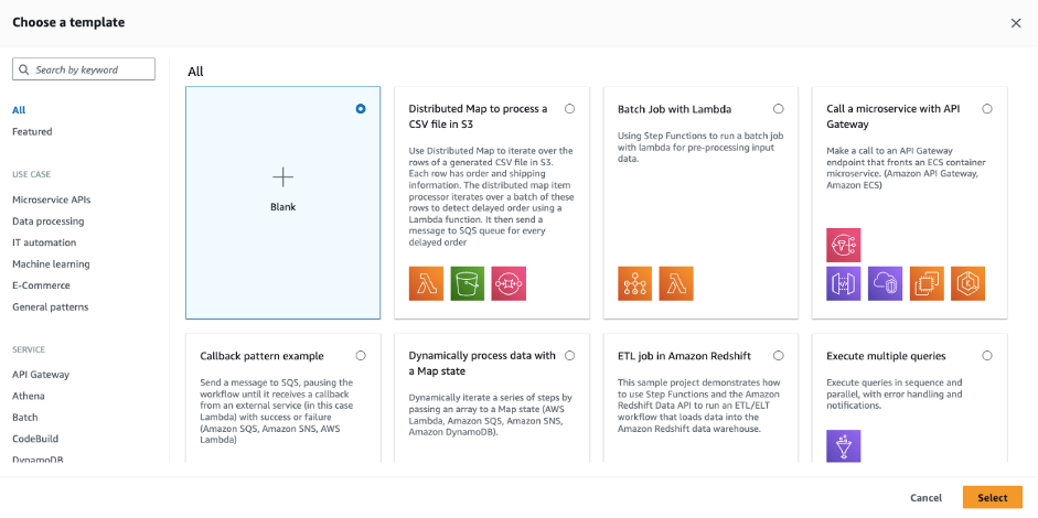
- This presents you with the new template selection. Search by keyword, or filter by use-case and service:

- Choose “Distributed Map to Process a CSV file in S3” and choose Select.
- The following view shows a visual representation of the workflow, along with a detailed description.

There are two usage options for each template:- Run a demo: Step Functions automatically deploys an AWS CloudFormation stack to your account, equipped with the state machine and all related resources. This ready-to-run demo workflow not only showcases the capabilities of your chosen template, but also serves as a springboard for your unique creations. Building upon this foundation, customize, fine tune, and tailor workflows to meet your exact specifications.
- Build on it: This places the workflow’s ASL into the new Workflow Studio code view. Importantly, this transition does not deploy any associated resources. The goal is to let you with an expedited workflow creation process that uses best practices templates, while allowing you to customize and adapt them to your specific needs without the need to build from scratch.
- Choose Run a demo, and then choose Use template. This places the workflow template into Workflow Studio in Read-only mode. Allowing you to inspect the workflow definition further before deploying the demo resources.
- To deploy the demo, choose Deploy and run:

After a few moments, the demo application is deployed to your account.


Seamless transitions between drag-and-drop design and code mode
Another enhancement in Workflow Studio is the ability to switch seamlessly between the drag-and-drop design view and the new code mode. This versatility allows you to transition between visual design and code-based authoring, catering to varying preferences and skill sets. While the design view offers an intuitive approach to creating workflows, the code mode provides a dynamic space akin to familiar coding environments.
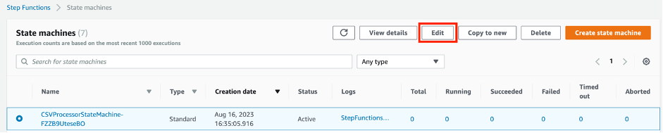
Open up the previously deployed workflow demo by selecting it from the state machines console and choosing Edit:
Choose the Code button to switch to the code authoring view:
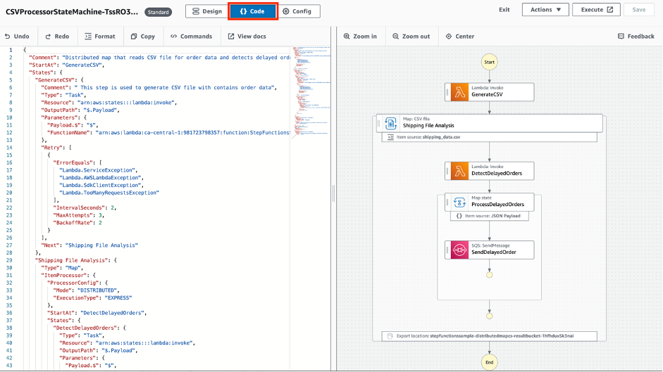
Here you are presented with an interface reminiscent of industry standard coding environments such as Visual Studio Code. This transformation lets experienced developers use the full potential of ASL enabling intricate customization and fine-tuning. It also allows you to use the graph visualization on the right to re-order easily and quickly, duplicate, or delete steps.
Chose the Design button to toggle back to the low code editor:
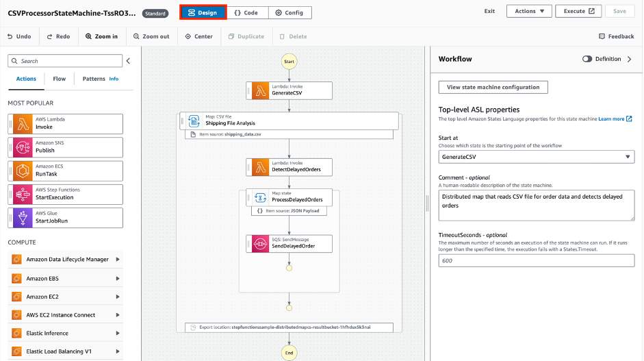
This is ideal for builders that are less experienced in ASL or for experienced developers needing to build workflow mocks rapidly, templates for further editing or prototype workflows.
Execute workflows directly from Workflow Studio
Workflow Studio now enables you to start a workflow from within the interface. This feature bridges the gap between design and execution, allowing developers to start their workflow from the Workflow Studio authoring environment.
To start a workflow from within Workflow Studio, choose the Execute button:
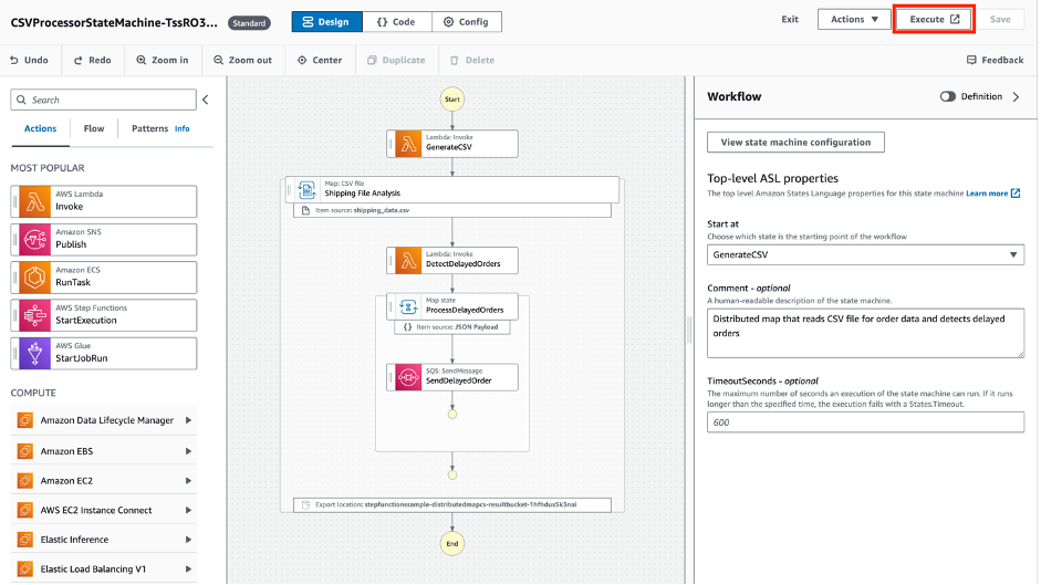
This takes you directly to the Step Functions executions interface where you can enter an input payload and inspect the workflow execution. This feature reduces the need to switch between interfaces, enabling developers to iterate more swiftly and efficiently. Choose Edit to jump directly back into Workflow Studio and continue iteratively refining your workflow.
Workflow Studio can now also view and edit execution role permissions, configure logging, and adjust additional parameters. To access this view, choose the Config button from Workflow Studio:

Availability for existing workflows
The new features are automatically available for all your existing workflows at no additional cost. This ensures that you can use the enhanced capabilities of Workflow Studio without any additional steps or configuration.
Workflow Studio’s new features allow developers to amplify their efforts. By simplifying the creation and execution of workflows, developers can channel more time and energy into the creative aspects of application development. Workflow Studio’s enhancements not only boost productivity but also provide a platform for turning creative designs into tangible, impactful applications.
Conclusion
Workflow Studio continues to evolve with the ongoing goal of simplifying and enhancing the process of building Step Functions workflows. The introduction of seamless authoring mode transitions, direct execution capabilities, and the improved starter template experience represents a pragmatic step towards improving authoring efficiency and flexibility, establishing Workflow Studio as the default authoring experience to Step Functions.
For additional starter templates, patterns, and best practices, visit the Serverless Workflows Collection on Serverless land.


 Raj Ramasubbu is a Senior Analytics Specialist Solutions Architect focused on big data and analytics and AI/ML with Amazon Web Services. He helps customers architect and build highly scalable, performant, and secure cloud-based solutions on AWS. Raj provided technical expertise and leadership in building data engineering, big data analytics, business intelligence, and data science solutions for over 18 years prior to joining AWS. He helped customers in various industry verticals like healthcare, medical devices, life science, retail, asset management, car insurance, residential REIT, agriculture, title insurance, supply chain, document management, and real estate.


 Prashant Agrawal is a Sr. Search Specialist Solutions Architect with Amazon OpenSearch Service. He works closely with customers to help them migrate their workloads to the cloud and helps existing customers fine-tune their clusters to achieve better performance and save on cost. Before joining AWS, he helped various customers use OpenSearch and Elasticsearch for their search and log analytics use cases. When not working, you can find him traveling and exploring new places. In short, he likes doing Eat → Travel → Repeat.


 Pavani Baddepudi is a Principal Product Manager for Search Services at AWS and the lead PM for OpenSearch Serverless. Her interests include distributed systems, networking, and security. When not working, she enjoys hiking and exploring new cuisines.
 Carl Meadows is Director of Product Management at AWS and is responsible for Amazon Elasticsearch Service, OpenSearch, Open Distro for Elasticsearch, and Amazon CloudSearch. Carl has been with Amazon Elasticsearch Service since before it was launched in 2015. He has a long history of working in the enterprise software and cloud services spaces. When not working, Carl enjoys making and recording music.


 Zack Rossman is a Member of Technical Staff at Alcion. He is the tech lead for the search and AI platforms. Prior to Alcion, Zack was a Senior Software Engineer at Okta, developing core workforce identity and access management products for the Directories team.
 Niraj Jetly is a Software Development Manager for Amazon OpenSearch Serverless. Niraj leads several data plane teams responsible for launching Amazon OpenSearch Serverless. Prior to AWS, Niraj led several product and engineering teams as CTO, VP of Engineering, and Head of Product Management for over 15 years. Niraj is a recipient of over 15 innovation awards, including being named CIO of the year in 2014 and top 100 CIO in 2013 and 2016. A frequent speaker at several conferences, he has been quoted in NPR, WSJ, and The Boston Globe.
 Jon Handler is a Senior Principal Solutions Architect at Amazon Web Services based in Palo Alto, CA. Jon works closely with OpenSearch and Amazon OpenSearch Service, providing help and guidance to a broad range of customers who have search and log analytics workloads that they want to move to the AWS Cloud. Prior to joining AWS, Jon’s career as a software developer included 4 years of coding a large-scale, ecommerce search engine. Jon holds a Bachelor of the Arts from the University of Pennsylvania and a Master of Science and a PhD in Computer Science and Artificial Intelligence from Northwestern University.


 Satesh Sonti is a Sr. Analytics Specialist Solutions Architect based out of Atlanta, specialized in building enterprise data platforms, data warehousing, and analytics solutions. He has over 17 years of experience in building data assets and leading complex data platform programs for banking and insurance clients across the globe.
 Harshida Patel is a Specialist Principal Solutions Architect, Analytics with AWS.
 Raghu Kuppala is an Analytics Specialist Solutions Architect experienced working in the databases, data warehousing, and analytics space. Outside of work, he enjoys trying different cuisines and spending time with his family and friends.
 Ashish Agrawal is a Sr. Technical Product Manager with Amazon Redshift, building cloud-based data warehouses and analytics cloud services. Ashish has over 24 years of experience in IT. Ashish has expertise in data warehouses, data lakes, and platform as a service. Ashish has been a speaker at worldwide technical conferences.


 Tamara Astakhova is a Sr. Partner Solutions Architect in Data and Analytics at AWS. She has over 18 years of experience in the architecture and development of large-scale data analytics systems. Tamara is working with strategic partners helping them build complex AWS-optimized architectures.
 Cameron Davie is a Principal Solutions Engineer for the Tech Alliances team. He oversees the technical responsibilities of Talend’s most strategic ISV partnerships. Cameron has been with Talend for 6 years in this role, working directly as the primary technical resource for partners such as AWS, Snowflake, and more. Cameron’s role at Talend is primarily focused on technical enablement and evangelism. This includes showcasing key capabilities of our partners’ solution internally as well as demonstrating Talend’s core technical capabilities with the technical sellers at Talend’s strategic ISV partners. Cameron is a veteran of ISV partnerships and enterprise software, with over 23 years of experience. Before Talend, he spent 14 years at SAP on their OEM/Embedded Solutions partnership team.