DevOps has revolutionized software development and operations by fostering collaboration, automation, and continuous improvement. By bringing together development and operations teams, organizations can accelerate software delivery, enhance reliability, and achieve faster time-to-market.
In this blog post, we will explore the best practices and architectural considerations for implementing DevOps with Amazon Web Services (AWS), enabling you to build efficient and scalable systems that align with DevOps principles. The Let’s Architect! team wants to share useful resources that help you to optimize your software development and operations.
Distributed systems are adopted from enterprises more frequently now. When an organization wants to leverage distributed systems’ characteristics, it requires a mindset and approach shift, akin to a new model for software development lifecycle.
In this re:Invent 2021 video, Emily Freeman, now Head of Community Engagement at AWS, shares with us the insights gained in the trenches when adapting a new software development lifecycle that will help your organization thrive using distributed systems.
Designing effective DevOps workflows is necessary for achieving seamless collaboration between development and operations teams. The Amazon Builders’ Library offers a wealth of guidance on designing DevOps workflows that promote efficiency, scalability, and reliability. From continuous integration and deployment strategies to configuration management and observability, this resource covers various aspects of DevOps workflow design. By following the best practices outlined in the Builders’ Library, you can create robust and scalable DevOps workflows that facilitate rapid software delivery and smooth operations.
Cloud fitness functions provide a powerful mechanism for driving evolutionary architecture within your DevOps practices. By defining and measuring architectural fitness goals, you can continuously improve and evolve your systems over time.
This AWS Architecture Blog post delves into how AWS services, like AWS Lambda, AWS Step Functions, and Amazon CloudWatch can be leveraged to implement cloud fitness functions effectively. By integrating these services into your DevOps workflows, you can establish an architecture that evolves in alignment with changing business needs: improving system resilience, scalability, and maintainability.
Achieving consistent deployments across multiple regions is a common challenge. This AWS DevOps Blog post demonstrates how to use Terraform, AWS CodePipeline, and infrastructure-as-code principles to automate Multi-Region deployments effectively. By adopting this approach, you can demonstrate the consistent infrastructure and application deployments, improving the scalability, reliability, and availability of your DevOps practices.
The post also provides practical examples and step-by-step instructions for implementing Multi-Region deployments with Terraform and AWS services, enabling you to leverage the power of infrastructure-as-code to streamline DevOps workflows.
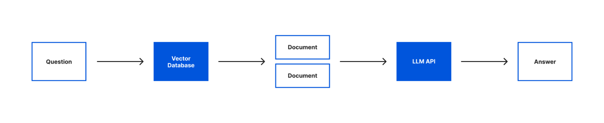
Amazon OpenSearch Serverless helps you index, analyze, and search your logs and data using OpenSearch APIs and dashboards. The OpenSearch Serverless collection is a group of indexes. API and dashboard clients can access the collections from public networks or one or more VPCs. For VPC access to collections and dashboards, you can create VPC endpoints. In this post, we demonstrate how you can create and use VPC endpoints and OpenSearch Serverless network policies to control access to your collections and OpenSearch dashboards from multiple network locations.
The demo in this post uses an AWS Lambda-based client in a VPC to ingest data into a collection via a VPC endpoint and a browser in a public network accessing the same collection.
Solution overview
To illustrate how you can ingest data into an OpenSearch Serverless collection from within a VPC, we use a Lambda function. We use a VPC-hosted Lambda function to create an index in an OpenSearch Serverless collection and add documents to the index using a VPC endpoint. We then use a publicly accessible OpenSearch Serverless dashboard to see the documents ingested from Lambda function.
The following sections detail the steps to ingest data into the collection using Lambda and access the OpenSearch Serverless dashboard.
Prerequisites
This setup assumes that you have already created a VPC with private subnets.
Ingest data using Lambda and access the OpenSearch Serverless dashboard
To set up your solution, complete the following steps:
On the OpenSearch Service console, create a private connection between your VPC and OpenSearch Serverless using a VPC endpoint. Use the private subnets and a security group from your VPC.
Create a network policy to enable VPC access to the OpenSearch endpoint so the Lambda function can ingest documents to the collection. You should also enable public access to the OpenSearch dashboard endpoint so we can see the documents ingested.
Additionally, grant read access to the dashboard user’s IAM role.
Add IAM permissions to the Lambda function’s IAM role and the dashboard user’s IAM role for the OpenSearch Serverless collection.
Create a Lambda function in the same VPC and subnet that we used for the OpenSearch endpoint (see the following code). This function creates an index called sitcoms-eighties in the OpenSearch Serverless collection and adds a sample document to the index:
import datetime
import time
from opensearchpy import OpenSearch, RequestsHttpConnection
from requests_aws4auth import AWS4Auth
import boto3

host = '<Insert-OpenSearch-Serverless-Endpoint>'
region = 'us-east-1'
service = 'aoss'
credentials = boto3.Session().get_credentials()
awsauth = AWS4Auth(credentials.access_key, credentials.secret_key, region, service,session_token=credentials.token)

# Build the OpenSearch client
client = OpenSearch(
    hosts=[{'host': host, 'port': 443}],
    http_auth=awsauth,
    use_ssl=True,
    verify_certs=True,
    connection_class=RequestsHttpConnection,
    timeout=300
)

def lambda_handler (event, context):

    # Create index
    response = client.indices.create('sitcoms-eighties')
    print('\nCreating index:')
    print(response)
    time.sleep(5)

    dt = datetime.datetime.now()
    # Add a document to the index.
    response = client.index(
        index='sitcoms-eighties',
        body={
            'title': 'Seinfeld',
            'creator': 'Larry David',
            'year': 1989,
            'createtime': dt
        },
        id='1',
    )
    print('\nDocument added:')
    print(response)
Run the Lambda function, and you should see the output as shown in the following screenshot.
You can now see the documents from this index through your publicly accessible OpenSearch Dashboards URL.
Create the index pattern in OpenSearch Dashboards, and then you can see the documents as shown in the following screenshot.
Use a VPC DNS resolver from your network
A client in your VPN network can connect to the collection or dashboards over a VPC endpoint. The client needs to find the VPC endpoint’s IP address using an Amazon Route 53 inbound resolver endpoint. To learn more about Route 53 inbound resolver endpoints, refer to Resolving DNS queries between VPCs and your network. The following diagram shows a sample setup.
The flow for this architecture is as follows:
The DNS query for the OpenSearch Serverless client is routed to a locally configured on-premises DNS server.
The on-premises DNS as configured performs conditional forwarding for the zone us-east-1.aoss.amazonaws.com to a Route 53 inbound resolver endpoint IP address. You must replace your Region name in the preceding zone name.
The inbound resolver endpoint performs DNS resolution by forwarding the query to the private hosted zone that was created along with the OpenSearch Serverless VPC endpoint.
The IP addresses returned by the DNS query are the private IP addresses of the interface VPC endpoint, which allow your on-premises host to establish private connectivity over AWS Site-to-Site VPN.
The interface endpoint is a collection of one or more elastic network interfaces with a private IP address in your account that serves as an entry point for traffic going to an OpenSearch Serverless endpoint.
Summary
OpenSearch Serverless allows you to set up and control access to the service using VPC endpoints and network policies. In this post, we explored how to access an OpenSearch Serverless collection API and dashboard from within a VPC, on premises, and public networks. If you have any questions or suggestions, please write to us in the comments section.
About the Authors
Raj Ramasubbu is a Senior Analytics Specialist Solutions Architect focused on big data and analytics and AI/ML with Amazon Web Services. He helps customers architect and build highly scalable, performant, and secure cloud-based solutions on AWS. Raj provided technical expertise and leadership in building data engineering, big data analytics, business intelligence, and data science solutions for over 18 years prior to joining AWS. He helped customers in various industry verticals like healthcare, medical devices, life science, retail, asset management, car insurance, residential REIT, agriculture, title insurance, supply chain, document management, and real estate.
Vivek Kansal works with the Amazon OpenSearch team. In his role as Principal Software Engineer, he uses his experience in the areas of security, policy engines, cloud-native solutions, and networking to help secure customer data in OpenSearch Service and OpenSearch Serverless in an evolving threat landscape.
This post is written by Gregor Hohpe, Sr. Principal Evangelist, Serverless.
Event-driven architectures (EDAs) help decouple applications or application components from one another. Consuming events makes a component less dependent on the sender’s location or implementation details. Because events are self-contained, they can be consumed asynchronously, which allows sender and receiver to follow independent timing considerations. Decoupling through events can improve development agility and operational resilience when building fine-grained distributed applications, which is the preferred style for serverless applications.
Many AWS services publish events through built-in mechanisms to support building event-driven architectures with a minimal amount of custom coding. Modern applications built on top of those services can also send and consume events based on their specific business logic. AWS application integration services like Amazon EventBridge or Amazon SNS, a managed publish-subscribe service, filter those events and route them to the intended destination, providing additional decoupling between event producer and consumer.
Publishing events
Custom applications that act as event producers often use the AWS SDK library, which is available for 12 programming languages, to send an event message. The application code constructs the event as a local data structure and specifies where to send it, for example to an EventBridge event bus.
The application code required to send an event to EventBridge is straightforward and only requires a few lines of code, as shown in this (simplified) helper method that publishes an order event generated by the application:
An application most likely calls such a method in the context of another action, for example when persisting a received order to a data store. The code that performs those tasks might look as follows:
The code populates an order object with multiple line items (in reality, this would be based on data entered by a user or received via an API call), writes it to a database (via another helper method whose implementation isn’t shown), and then sends it to an EventBridge bus via the preceding method.
Code causes coupling
Although this code is not complex, it has drawbacks from an architectural perspective:
It interweaves application logic with the solution’s topology because the destination of the event, both in terms of service (EventBridge versus SNS, for example) and the instance (the service bus name in this case) are defined inside the application’s source code. If the event destination changes, you must change the source code, or at least know which string constant is passed to the function via an environment variable. Both aspects work against the EDA principle of minimizing coupling between components because changes in the communication structure propagate into the producer’s source code.
Sending the event after updating the database is brittle because it lacks transactional guarantees across both steps. You must implement error handling and retry logic to handle cases where sending the event fails, or even undo the database update. Writing such code can be tedious and error-prone.
Code is a liability. After all, that’s where bugs come from. In a real-life example, a helper method similar to preceding code erroneously swapped day and month on the event date, which led to a challenging debugging cycle. Boilerplate code to send events is therefore best avoided.
Performing event routing inside EventBridge can lessen the first concern. You could reconfigure EventBridge’s rules and targets to route events with a specified type and source to a different destination, provided you keep the event bus name stable. However, the other issues would remain.
Serverless: Less infrastructure, less code
AWS serverless integration services can alleviate the need to write custom application code to publish events altogether.
A key benefit of serverless applications is that you can let the AWS Cloud do the undifferentiated heavy lifting for you. Traditionally, we associate serverless with provisioning, scaling, and operating compute infrastructure so that developers can focus on writing code that generates business value.
Serverless application integration services can also take care of application-level tasks for you, including publishing events. Most applications store data in AWS data stores like Amazon Simple Storage Service (S3) or Amazon DynamoDB, which can automatically emit events whenever an update takes place, without any application code.
EventBridge Pipes: Events without application code
EventBridge Pipes allows you to create point-to-point integrations between event producers and consumers with optional transformation, filtering, and enrichment steps. Serverless integration services combined with cloud automation allow ”point-to-point” integrations to be more easily managed than in the past, which makes them a great fit for this use case.
This example takes advantage of EventBridge Pipes’ ability to fetch events actively from sources like DynamoDB Streams. DynamoDB Streams captures a time-ordered sequence of item-level modifications in any DynamoDB table and stores this information in a log for up to 24 hours. EventBridge Pipes picks up events from that log and pushes them to one of over 14 event targets, including an EventBridge bus, SNS, SQS, or API Destinations. It also accommodates batch sizes, timeouts, and rate limiting where needed.
The integration through EventBridge Pipes can replace the custom application code that sends the event, including any retry or error logic. Only the following code remains:
EventBridge Pipes can be configured from the CLI, the AWS Management Console, or from automation code using AWS CloudFormation or AWS CDK. By using AWS CDK, you can use the same programming language that you use to write your application logic to also write your automation code.
For example, the following CDK snippet configures an EventBridge Pipe to read events from a DynamoDB Stream attached to the Orders table and passes them to an EventBridge event bus.
This code references the DynamoDB table via the ordersTable variable that would be set when the table is created:
The automation code cleanly defines the dependency between the DynamoDB table and the event destination, independent of application logic.
Decoupling with data transformation
Coupling is not limited to event sources and destinations. A source’s data format can determine the event format and require downstream changes in case the data format or the data source change. EventBridge Pipes can also alleviate that consideration.
Events emitted from the DynamoDB Stream use the native, marshaled DynamoDB format that includes type information, such as an “S” for strings or “L” for lists.
For example, the order event in the DynamoDB stream from this example looks as follows. Some fields are omitted for readability:
This format is not well suited for downstream processing because it would unnecessarily couple event consumers to the fact that this event originated from a DynamoDB Stream. EventBridge Pipes can convert this event into a more easily consumable format. The transformation is specified via an inputTemplate parameter using JSONPath expressions. EventBridge Pipes added support for list processing with wildcards proves to be perfect for this scenario.
In this example, add the following transformation template inside the target parameters to the preceding CDK code (the asterisk character matches a complete list of elements):
This transformation formats the event published by EventBridge Pipes like a regular business event, decoupling any event consumer from the fact that it originated from a DynamoDB table:
When building event-driven applications, consider whether you can replace application code with serverless integration services to improve the resilience of your application and provide a clean separation between application logic and system dependencies.
EventBridge Pipes can be a helpful feature in these situations, for example to capture and publish events based on DynamoDB table updates.
This post is written by Pawan Puthran, Principal Serverless Specialist TAM, Aneel Murari, Senior Serverless Specialist Solution Architect, and Shree Shrikhande, Senior AWS Lambda Product Manager.
AWS Lambda is announcing a recursion control to detect and stop Lambda functions running in a recursive or infinite loop.
At launch, this feature is available for Lambda integrations with Amazon Simple Queue Service (Amazon SQS), Amazon SNS, or when invoking functions directly using the Lambda invoke API. Lambda now detects functions that appear to be running in a recursive loop and drops requests after exceeding 16 invocations.
This can help reduce costs from unexpected Lambda function invocations because of recursion. You receive notifications about this action through the AWS Health Dashboard, email, or by configuring Amazon CloudWatch Alarms.
Overview
You can invoke Lambda functions in multiple ways. AWS services generate events that invoke Lambda functions, and Lambda functions can send messages to other AWS services. In most architectures, the service or resource that invokes a Lambda function should be different from the service or resource that the function outputs to. Because of misconfiguration or coding bugs, a function can send a processed event to the same service or resource that invokes the Lambda function, causing a recursive loop.
Lambda now detects the function running in a recursive loop between supported services, after exceeding 16 invocations. It returns a RecursiveInvocationException to the caller. There is no additional charge for this feature. For asynchronous invokes, Lambda sends the event to a dead-letter queue or on-failure destination, if one is configured.
The following is an example of an order processing system.
Order processing system
A new order information message is sent to the source SQS queue.
Lambda consumes the message from the source queue using an ESM.
The Lambda function processes the message and sends the updated orders message to a destination SQS queue using the SQS SendMessage API.
The source queue has a dead-letter queue(DLQ) configured for handling any failed or unprocessed messages.
Because of a misconfiguration, the Lambda function sends the message to the source SQS queue instead of the destination queue. This causes a recursive loop of Lambda function invocations.
To explore sample code for this example, see the GitHub repo.
In the preceding example, after 16 invocations, Lambda throws a RecursiveInvocationException to the ESM. The ESM stops invoking the Lambda function and, once the maxReceiveCount is exceeded, SQS moves the message to the source queues configured DLQ.
You receive an AWS Health Dashboard notification with steps to troubleshoot the function.
AWS Health Dashboard notification
You also receive an email notification to the registered email address on the account.
Email notification
Lambda emits a RecursiveInvocationsDropped CloudWatch metric, which you can view in the CloudWatch console.
RecursiveInvocationsDropped CloudWatch metric
How does Lambda detect recursion?
For Lambda to detect recursive loops, your function must use one of the supported AWS SDK versions or higher.
Lambda uses an AWS X-Ray trace header primitive called “Lineage” to track the number of times a function has been invoked with an event. When your function code sends an event using a supported AWS SDK version, Lambda increments the counter in the lineage header. If your function is then invoked with the same triggering event more than 16 times, Lambda stops the next invocation for that event. You do not need to configure active X-Ray tracing for this feature to work.
43e12f0f is the hash of a resource, in this case a Lambda function. 5 is the number of times this function has been invoked with the same event. The logic of hash generation, encoding, and size of the lineage header may change in the future. You should not design any application functionality based on this.
When using an ESM to consume messages from SQS, after the maxReceiveCount value is exceeded, the message is sent to the source queue’s configured DLQ. When Lambda detects a recursive loop and drops subsequent invocations, it returns a RecursiveInvocationException to the ESM. This increments the maxReceiveCount value. When the ESM auto retries to process events, based on the error handling configuration, these retries are not considered recursive invocations.
When using SQS, you can also batch multiple messages into one Lambda event. Where the message batch size is greater than 1, Lambda uses the maximum lineage value within the batch of messages. It drops the entire batch if the value exceeds 16.
Recursion detection in action
You can deploy a sample application example in the GitHub repo to test Lambda recursive loop detection. The application includes a Lambda function that reads from an SQS queue and writes messages back to the same SQS queue.
git clone https://github.com/aws-samples/aws-lambda-recursion-detection-sample.git
cd aws-lambda-recursion-detection-sample
Use AWS SAM to build and deploy the resources to your AWS account. Enter a stack name, such as lambda-recursion, when prompted. Accept the remaining default values.
sam build –-use-container
sam deploy --guided --region $REGION
To test the application:
Save the name of the SQS queue in a local environment variable:
This invokes the Lambda function, which writes the message back to the queue.
To verify that Lambda has detected the recursion:
Navigate to the CloudWatch console. Choose All Metrics under Metrics in the left-hand panel and search for RecursiveInvocationsDropped.
Find RecursiveInvocationsDropped.
Choose Lambda > By Function Name and choose RecursiveInvocationsDropped for the function you created. Under Graphed metrics, change the statistic to sum and Period to 1 minute. You see one record. Refresh if you don’t see the metric after a few seconds.
Metrics sum view
Actions to take when Lambda stops a recursive loop
When you receive a notification regarding recursion in your account, the following steps can help address the issue.
To stop further invoke attempts while you fix the underlying configuration issue, set the function concurrency to 0. This acts as an off switch for the Lambda function. You can choose the “Throttle” button in the Lambda console or use the PutFunctionConcurrency API to set the function concurrency to 0.
You can also disable or delete the event source mapping or trigger for the Lambda function.
Check your Lambda function code and configuration for any code defects that create loops. For example, check your environment variables to ensure you are not using the same SQS queue or SNS topic as source and target.
If an SQS Queue is the event source for your Lambda function, configure a DLQ on the source queue.
If an SNS topic is the event source, configure an On-Failure Destination for the Lambda function.
Disabling recursion detection
You may have valid use-cases where Lambda recursion is intentional as part of your design. In this case, use caution and implement suitable guardrails to prevent unexpected charges to your account. To learn more about best practices for using recursive invocation patterns, see Recursive patterns that cause run-away Lambda functions in the AWS Lambda Operator Guide.
This feature is turned on by default to stop recursive loops. To request turning it off for your account, reach out to AWS Support.
Conclusion
Lambda recursion control for SQS and SNS automatically detects and stops functions running in a recursive or infinite loop. This can be due to misconfiguration or coding errors. Recursion control helps reduce unexpected usage with Lambda and downstream services. The post also explains how Lambda detects and stops recursive loops and notifies you through AWS Health Dashboard to troubleshoot the function.
This post is written by Archana Srikanta, Principal Engineer, AWS Lambda.
When you call AWS Lambda’s Invoke API, a series of throttle limits are evaluated to decide if your call is let through or throttled with a 429 “Too Many Requests” exception. This blog post explains the most common invoke throttle limits and the relationship between them, so you can better understand scaling workloads on Lambda.
Overview
The throttle limits exist to protect the following components of Lambda’s internal service architecture, and your workload, from noisy neighbors:
Execution environment: An execution environment is a Firecracker microVM where your function code runs. A given execution environment only hosts one invocation at a time, but it can be reused for subsequent invocations of the same function version.
Invoke data plane: These are a series of internal web services that, on an invoke, select (or create) a sandbox and route your request to it. This is also responsible for enforcing the throttle limits.
When you make an Invoke API call, it transits through some or all of the Invoke Data Plane services, before reaching an execution environment where your function code is downloaded and executed.
There are three distinct but related throttle limits which together decide if your invoke request is accepted by the data plane or throttled.
Concurrency
Concurrent means “existing, happening, or done at the same time”. Accordingly, the Lambda concurrency limit is a limit on the simultaneous in-flight invocations allowed at any given time. It is not a rate or transactions per second (TPS) limit in and of itself, but instead a limit on how many invocations can be inflight at the same time. This documentation visually explains the concept of concurrency.
Under the hood, the concurrency limit roughly translates to a limit on the maximum number of execution environments (and thus Firecracker microVMs) that your account can claim at any given point in time. Lambda runs a fleet of multi-tenant bare metal instances, on which Firecracker microVMs are carved out to serve as execution environments for your functions. AWS constantly monitors and scales this fleet based on incoming demand and shares the available capacity fairly among customers.
The concurrency limit helps protect Lambda from a single customer exhausting all the available capacity and causing a denial of service to other customers.
Transactions per second (TPS)
Customers often ask how their concurrency limit translates to TPS. The answer depends on how long your function invocations last.
The diagram above considers three cases, each with a different function invocation duration, but a fixed concurrency limit of 1000. In the first case, invocations have a constant duration of 1 second. This means you can initiate 1000 invokes and claim all 1000 execution environments permitted by your concurrency limit. These execution environments remain busy for the entire second, and you cannot start any more invokes in that second because your concurrency limit prevents you from claiming any more execution environments. So, the TPS you can achieve with a concurrency limit of 1000 and a function duration of 1 second is 1000 TPS.
In case 2, the invocation duration is halved to 500ms, with the same concurrency limit of 1000. You can initiate 1000 concurrent invokes at the start of the second as before. These invokes keep the execution environments busy for the first half of the second. Once finished, you can start an additional 1000 invokes against the same execution environments while still being within your concurrency limit. So, by halving the function duration, you doubled your TPS to 2000.
Similarly, in case 3, if your function duration is 100ms, you can initiate 10 rounds of 1000 invokes each in a second, achieving a TPS of 10K.
Codifying this as an equation, the TPS you can achieve given a concurrency limit is:
TPS = concurrency / function duration in seconds
Taken to an extreme, for a function duration of only 1ms and at a concurrency limit of 1000 (the default limit), an account can drive an invoke TPS of one million. For every additional unit of concurrency granted via a limit increase, it implicitly grants an additional 1000 TPS per unit of concurrency increased. The high TPS doesn’t require any additional execution environments (Firecracker microVMs), so it’s not problematic from a fleet capacity perspective. However, driving over a million TPS from a single account puts stress on the Invoke Data Plane services. They must be protected from noisy neighbor impact as well so all customers have a fair share of the services’ bandwidth. A concurrency limit alone isn’t sufficient to protect against this – the TPS limit provides this protection.
As of this writing, the invoke TPS is capped at 10 times your concurrency. Added to the previous equation:
TPS = min( 10 x concurrency, concurrency / function duration in seconds)
The concurrency factor is common across both terms in the min function, so the key comparison is:
min(10, 1 / function duration in seconds)
If the function duration is exactly 100ms (or 1/10th of a second), both terms in the min function are equal. If the function duration is over 100ms, the second term is lower and TPS is limited as per concurrency/function duration. If the function duration is under 100ms, the first term is lower and TPS is limited as per 10 x concurrency.
To summarize, the TPS limit exists to protect the Invoke Data Plane from the high churn of short-lived invocations, for which the concurrency limit alone affords too high of a TPS. If you drive short invocations of under 100ms, your throughput is capped as though the function duration is 100ms (at 10 x concurrency) as shown in the diagram above. This implies that short lived invocations may be TPS limited, rather than concurrency limited. However, if your function duration is over 100ms you can effectively ignore the 10 x concurrency TPS limit and calculate your available TPS as concurrency/function duration.
Burst
The third throttle limit is the burst limit. Lambda does not keep execution environments provisioned for your entire concurrency limit at all times. That would be wasteful, especially if usage peaks are transient, as is the case with many workloads. Instead, the service spins up execution environments just-in-time as the invoke arrives, if one doesn’t already exist. Once an execution environment is spun up, it remains “warm” for some period of time and is available to host subsequent invocations of the same function version.
However, if an invoke doesn’t find a warm execution environment, it experiences a “cold start” while we provision a new execution environment. Cold starts involve certain additional operations over and above the warm invoke path, such as downloading your code or container and initializing your application within the execution environment. These initialization operations are typically computationally heavy and so have a lower throughput compared to the warm invoke path. If there are sudden and steep spikes in the number of cold starts, it can put pressure on the invoke services that handle these cold start operations, and also cause undesirable side effects for your application such as increased latencies, reduced cache efficiency and increased fan out on downstream dependencies. The burst limit exists to protect against such surges of cold starts, especially for accounts that have a high concurrency limit. It ensures that the climb up to a high concurrency limit is gradual so as to smooth out the number of cold starts in a burst.
The algorithm used to enforce the burst limit is the Token Bucket rate-limiting algorithm. Consider a bucket that holds tokens. The bucket has a maximum capacity of B tokens (burst). The bucket starts full. Each time you send an invoke request that requires an additional unit of concurrency, it costs a token from the bucket. If the token exists, you are granted the additional concurrency and the token is removed from the bucket. The bucket is refilled at a constant rate of r tokens per minute (rate) until it reaches its maximum capacity.
What this means is that the rate of climb of concurrency is limited to r tokens per minute. Even though the algorithm allows you to collect up to B tokens and burst, you must wait for the bucket to refill before you can burst again, effectively limiting your average rate to r per minute.
The chart above shows the burst limit in action with a maximum concurrency limit of 3000, a maximum burst(B) of 1000 and a refill rate(r) of 500/minute. The token bucket starts full with 1000 tokens, as is the available burst headroom.
There is a burst activity between minute one and two, which consumes all tokens in the bucket and claims all 1000 concurrent execution environments allowed by the burst limit. At this point the bucket is empty and any attempt to claim additional concurrent execution environments is burst throttled, in spite of max concurrency not being reached yet.
The token bucket and the burst headroom are replenished at minutes two and three with 500 tokens each minute to bring it back up to its maximum capacity of 1000. At minute four, there is no additional refill because the bucket is at maximum capacity. Between minutes four and five, there is a second burst activity which empties the bucket again and claims an additional 1000 execution environments, bringing the total number of active execution environments to 2000.
The bucket continues to replenish at a rate of 500/minute at minutes five and six. At this point, sufficient tokens have been accumulated to cover the entire concurrency limit of 3000, and so the bucket isn’t refilled anymore even when you have the third burst activity at minute seven. At minute ten, when all the usage ramps down, the available burst headroom slowly stair steps back down to the maximum initial burst of 1K.
The actual numbers for maximum burst and refill rate vary by Region and are subject to change, please visit the Lambda burst limits page for specific values.
It is important to distinguish that the burst limit isn’t a rate limit on the invoke itself, but a rate limit on how quickly concurrency can rise. However, since invoke TPS is a function of concurrency, it also clamps how quickly TPS can rise (a rate limit for a rate limit). The following chart shows how the TPS burst headroom follows a similar stair step pattern as the concurrency burst headroom, only with a multiplier.
Conclusion
This blog explains three key throttle limits applied on Lambda invokes: the concurrency limit, TPS limit and burst limit. It outlines the relationship between these limits and how each one protects the system and your workload from noisy neighbors. Equipped with this knowledge you can better interpret any 429 throttling exceptions you may receive while scaling your applications on Lambda. For more information on getting started with Lambda visit the Developer Guide.
For more serverless learning resources, visit Serverless Land.
This post is written by Jeff Chen, Principal Cloud Application Architect, and Jeff Li, Senior Cloud Application Architect
Event-driven architectures are an architecture style that can help you boost agility and build reliable, scalable applications. Splitting an application into loosely coupled services can help each service scale independently. A distributed, loosely coupled application depends on events to communicate application change states. Each service consumes events from other services and emits events to notify other services of state changes.
Handling errors becomes even more important when designing distributed applications. A service may fail if it cannot handle an invalid payload, dependent resources may be unavailable, or the service may time out. There may be permission errors that can cause failures. AWS services provide many features to handle error conditions, which you can use to improve the resiliency of your applications.
This post explores three use-cases and design patterns for handling failures.
Lambda’s integration with Amazon API Gateway is an example of a synchronous invocation. A client makes a request to API Gateway, which sends the request to Lambda. API Gateway waits for the function response and returns the response to the client. There are no built-in retries or error handling. If the request fails, the client attempts the request again.
Lambda’s integration with SNS and EventBridge are examples of asynchronous invocations. SNS, for example, sends an event to Lambda for processing. When Lambda receives the event, it places it on an internal event queue and returns an acknowledgment to SNS that it has received the message. Another Lambda process reads events from the internal queue and invokes your Lambda function. If SNS cannot deliver an event to your Lambda function, the service automatically retries the same operation based on a retry policy.
Lambda’s integration with SQS uses poll-based invocations. Lambda runs a fleet of pollers that poll your SQS queue for messages. The pollers read the messages in batches and invoke your Lambda function once per batch.
You can apply this pattern in many scenarios. For example, your operational application can add sales orders to an operational data store. You may then want to load the sales orders to your data warehouse periodically so that the information is available for forecasting and analysis. The operational application can batch completed sales as events and place them on an SQS queue. A Lambda function can then process the events and load the completed sale records into your data warehouse.
If your function processes the batch successfully, the pollers delete the messages from the SQS queue. If the batch is not successfully processed, the pollers do not delete the messages from the queue. Once the visibility timeout expires, the messages are available again to be reprocessed. If the message retention period expires, SQS deletes the message from the queue.
The following table shows the invocation types and retry behavior of the AWS services mentioned.
AWS service example
Invocation type
Retry behavior
Amazon API Gateway
Synchronous
No built-in retry, client attempts retries.
Amazon SNS
Amazon EventBridge
Asynchronous
Built-in retries with exponential backoff.
Amazon SQS
Poll-based
Retries after visibility timeout expires until message retention period expires.
There are a number of design patterns to use for poll-based and asynchronous invocation types to retain failed messages for additional processing. These patterns can help you recover from delivery or processing failures.
When using Lambda with SQS, if Lambda isn’t able to process the message and the message retention period expires, SQS drops the message. Failure to process the message can be due to function processing failures, including time-outs or invalid payloads. Processing failures can also occur when the destination function does not exist, or has incorrect permissions.
You can configure a separate dead-letter queue (DLQ) on the source queue for SQS to retain the dropped message. A DLQ preserves the original message and is useful for analyzing root causes, handling error conditions properly, or sending notifications that require manual interventions. In the poll-based invocation scenario, the Lambda function itself does not maintain a DLQ. It relies on the external DLQ configured in SQS. For more information, see Using Lambda with Amazon SQS.
The following shows the design pattern when you configure Lambda to poll events from an SQS queue and invoke a Lambda function.
Lambda synchronously polling batches of messages from SQS
To explore this pattern, deploy the code in this repository. Once deployed, you can use this instruction to test the pattern with the happy and unhappy paths.
Lambda asynchronous invocation pattern
With asynchronous invokes, there are two failure aspects to consider when using Lambda. The event source cannot deliver the message to Lambda and the Lambda function errors when processing the event.
Event sources vary in how they handle failures delivering messages to Lambda. If SNS or EventBridge cannot send the event to Lambda after exhausting all their retry attempts, the service drops the event. You can configure a DLQ on an SNS topic or EventBridge event bus to hold the dropped event. This works in the same way as the poll-based invocation pattern with SQS.
Lambda functions may then error due to input payload syntax errors, duration time-outs, or the function throws an exception such as a data resource not available.
For asynchronous invokes, you can configure how long Lambda retains an event in its internal queue, up to 6 hours. You can also configure how many times Lambda retries when the function errors, between 0 and 2. Lambda discards the event when the maximum age passes or all retry attempts fail. To retain a copy of discarded events, you can configure either a DLQ or, preferably, a failed-event destination as part of your Lambda function configuration.
A Lambda destination enables you to specify what to do next if an asynchronous invocation succeeds or fails. You can configure a destination to send invocation records to SQS, SNS, EventBridge, or another Lambda function. Destinations are preferred for failure processing as they support additional targets and include additional information. A DLQ holds the original failed event. With a destination, Lambda also passes details of the function’s response in the invocation record. This includes stack traces, which can be useful for analyzing the root cause.
Using both a DLQ and Lambda destinations
You can apply this pattern in many scenarios. For example, many of your applications may contain customer records. To comply with the California Consumer Privacy Act (CCPA), different organizations may need to delete records for a particular customer. You can set up a consumer delete SNS topic. Each organization creates a Lambda function, which processes the events published by the SNS topic and deletes customer records in its managed applications.
The following shows the design pattern when you configure an SNS topic as the event source for a Lambda function, which uses destination queues for success and failure process.
SNS topic as event source for Lambda
You configure a DLQ on the SNS topic to capture messages that SNS cannot deliver to Lambda. When Lambda invokes the function, it sends details of the successfully processed messages to an on-success SQS destination. You can use this pattern to route an event to multiple services for simpler use cases. For orchestrating multiple services, AWS Step Functions is a better design choice.
Lambda can also send details of unsuccessfully processed messages to an on-failure SQS destination.
A variant of this pattern is to replace an SQS destination with an EventBridge destination so that multiple consumers can process an event based on the destination.
To explore how to use an SQS DLQ and Lambda destinations, deploy the code in this repository. Once deployed, you can use this instruction to test the pattern with the happy and unhappy paths.
Using a DLQ
Although destinations is the preferred method to handle function failures, you can explore using DLQs.
The following shows the design pattern when you configure an SNS topic as the event source for a Lambda function, which uses SQS queues for failure process.
Lambda invoked asynchonously
You configure a DLQ on the SNS topic to capture the messages that SNS cannot deliver to the Lambda function. You also configure a separate DLQ for the Lambda function. Lambda saves an unsuccessful event to this DLQ after Lambda cannot process the event after maximum retry attempts.
To explore how to use a Lambda DLQ, deploy the code in this repository. Once deployed, you can use this instruction to test the pattern with happy and unhappy paths.
Conclusion
This post explains three patterns that you can use to design resilient event-driven serverless applications. Error handling during event processing is an important part of designing serverless cloud applications.
You can deploy the code from the repository to explore how to use poll-based and asynchronous invocations. See how poll-based invocations can send failed messages to a DLQ. See how to use DLQs and Lambda destinations to route and handle unsuccessful events.
Learn more about event-driven architecture on Serverless Land.
Welcome to the 22nd edition of the AWS Serverless ICYMI (in case you missed it) quarterly recap. Every quarter, we share all the most recent product launches, feature enhancements, blog posts, webinars, live streams, and other interesting things that you might have missed!
In case you missed our last ICYMI, check out what happened last quarter here.
Serverless Land, your go-to resource for all things serverless, expanded to include a new Serverless Testing section. This provides valuable insights, patterns, and best practices for testing integrations using AWS SAM and CDK templates.
Serverless Land also launched a new learning page featuring a collection of resources, including blog posts, videos, workshops, and training materials, allowing users to choose a learning path from a variety of topics. “EventBridge Visuals“, small, easily digestible visuals focused on EventBridge have also been added.
AWS Lambda
Lambda introduced support for response payload streaming allowing functions to progressively stream response data to clients. This feature significantly improves performance by reducing the time to first byte (TTFB) latency, benefiting web and mobile applications.
Response streaming is particularly useful for applications with large payloads such as images, videos, documents, or database results. It eliminates the need to buffer the entire payload in memory and enables the transfer of responses larger than Lambda’s 6 MB limit, up to a soft limit of 20 MB.
By configuring the Function URL to use the InvokeWithResponseStream API, streaming responses can be accessed through an HTTP client that supports incremental response data. This enhancement expands Lambda’s capabilities, allowing developers to handle larger payloads more efficiently and enhance the overall performance and user experience of their web and mobile applications.
Lambda now supports Java 17 with Amazon Corretto distribution, providing long-term support and improved performance. Java 17 introduces new language features like records, sealed classes, and multi-line strings. The runtime uses ZGC and Shenandoah garbage collectors to reduce latency. Default JVM configuration changes optimize tiered compilation for reduced startup latency. Developers can use Java 17 in Lambda through AWS Management Console, AWS SAM, and AWS CDK. Popular frameworks like Spring Boot 3 and Micronaut 4 require Java 17 as a minimum. Micronaut provides a web service to generate example projects using Java 17 and AWS CDK infrastructure.
Lambda now supports the Ruby 3.2 runtime, enabling you to write serverless functions using the latest version of the Ruby programming language. This update enhances developer productivity and brings new features and improvements to your Ruby-based Lambda functions.
The latest update to AWS Step Functionsintroduces versions and aliases, allows users to run specific state machine revisions, ensuring reliable deployments, reducing risks, and providing version visibility. Appending version numbers to the state machine ARN enables selection of desired versions, even after updates. Aliases distribute execution requests based on weights, supporting incremental deployment patterns.
This enhances confidence in state machine updates, improves observability, auditing, and can be managed through the Step Functions console or AWS CloudFormation. Versions and aliases are available in all supported AWS Regions at no extra cost.
AWS SAM
AWS SAM CLI has introduced a new feature called remote invoke that allows developers to test Lambda functions in the AWS Cloud. This feature enables developers to invoke Lambda functions from their local development environment and provides options for event payloads, output formats, and logging.
It can be used with or without AWS SAM and can be combined with AWS SAM Accelerate for streamlined development and testing. Overall, the remote invoke feature simplifies serverless application testing in the AWS Cloud.
Amazon EventBridge
EventBridge announced an open-source connector for Kafka Connect, providing seamless integration between EventBridge and Kafka Connect. This connector simplifies the process of streaming events from Kafka topics to EventBridge, enabling you to build event-driven architectures with ease.
EventBridge has improved end-to-end latencies for event buses, delivering events up to 80% faster. This enables broader use in latency-sensitive applications such as industrial and medical applications, with the lower latencies applied by default across all AWS Regions at no extra cost.
Amazon Aurora Serverless v2
Amazon Aurora Serverless v2 is now available in four additional Regions, expanding the reach of this scalable and cost-effective serverless database option. With Aurora Serverless v2, you can benefit from automatic scaling, pause-and-resume capability, and pay-per-use pricing, enabling you to optimize costs and manage your databases more efficiently.
Amazon SNS
Amazon SNS now supports message data protection in five additional Regions, ensuring the security and integrity of your message payloads. With this feature, you can encrypt sensitive message data at rest and in transit, meeting compliance requirements and safeguarding your data.
Weekly live virtual office hours. In each session we talk about a specific topic or technology related to serverless and open it up to helping you with your real serverless challenges and issues.
The Serverless landing page has more information. The Lambda resources page contains case studies, webinars, whitepapers, customer stories, reference architectures, and even more Getting Started tutorials.
You can also follow the Serverless Developer Advocacy team on Twitter to see the latest news, follow conversations, and interact with the team.
This post is written by Andrea Amorosi, Senior Solutions Architect and Pascal Vogel, Solutions Architect.
When building serverless applications using AWS Lambda, you often need to retrieve parameters, such as database connection details, API secrets, or global configuration values at runtime. You can make these parameters available to your Lambda functions via secure, scalable, and highly available parameter stores, such as AWS Systems Manager Parameter Store or AWS Secrets Manager.
The Parameters utility for Powertools for AWS Lambda (TypeScript) simplifies the integration of these parameter stores inside your Lambda functions. The utility provides high-level functions for retrieving secrets and parameters, integrates caching and transformations, and reduces the amount of boilerplate code you must write.
The Parameters utility supports the following parameter stores:
This blog post shows how to use the new Parameters utility to retrieve parameters and secrets in your JavaScript and TypeScript Lambda functions securely.
Getting started with the Parameters utility
Initial setup
The Powertools toolkit is modular, meaning that you can install the Parameters utility independently from the Logger, Tracing, or Metrics packages. Install the Parameters utility library in your project via npm:
npm install @aws-lambda-powertools/parameters
In addition, you must add the AWS SDK client for the parameter store you are planning to use. The Parameters utility supports AWS SDK v3 for JavaScript only, which allows the utility to be modular. You install only the needed SDK packages to keep your bundle size small.
The following sections illustrate how to perform the previously mentioned steps for some typical parameter retrieval scenarios.
Retrieving a single parameter from SSM Parameter Store
To retrieve parameters from SSM Parameter Store, install the AWS SDK client for SSM in addition to the Parameters utility:
npm install @aws-sdk/client-ssm
To retrieve an individual parameter, the Parameters utility provides the getParameter function:
import { getParameter } from '@aws-lambda-powertools/parameters/ssm';

export const handler = async (): Promise<void> => {
  // Retrieve a single parameter
  const parameter = await getParameter('/my/parameter');
  console.log(parameter);
};
Finally, you need to assign an IAM policy with the ssm:GetParameter permission to your Lambda function execution role. Apply the principle of least privilege by scoping the permission to the specific parameter resource as shown in the following policy example:
By default, the retrieved parameters are cached in-memory for 5 seconds. This cached value is used for further invocations of the Lambda function until it expires. If your application requires a different behavior, the Parameters utility allows you to adjust the time-to-live (TTL) via the maxAge argument.
Building on the previous example, if you want to cache your retrieved parameter for 30 instead of 5 seconds, you can adapt your function code as follows:
import { getParameter } from '@aws-lambda-powertools/parameters/ssm';

export const handler = async (): Promise<void> => {
  // Retrieve a single parameter with a 30 seconds cache TTL
  const parameter = await getParameter('/my/parameter', { maxAge: 30 });
  console.log(parameter);
};
In other cases, you may want to always retrieve the latest value from the parameter store and ignore any cached value. To achieve this, set the forceFetch parameter to true:
import { getParameter } from '@aws-lambda-powertools/parameters/ssm';

export const handler = async (): Promise<void> => {
  // Always retrieve the latest value of a single parameter
  const parameter = await getParameter('/my/parameter', { forceFetch: true });
  console.log(parameter);
};
For details, see Always fetching the latest in the Powertools for AWS Lambda (TypeScript) documentation.
Decoding parameters stored in JSON or base64 format
If some of your parameters are stored in base64 or JSON, you can deserialize them via the Parameters utility’s transform argument.
Considering a parameter stored in SSM as JSON, it can be retrieved and deserialized as follows:
import { Transform } from '@aws-lambda-powertools/parameters';
import { getParameter } from '@aws-lambda-powertools/parameters/ssm';

export const handler = async (): Promise => {
  // Retrieve and deserialize a single JSON parameter
  const valueFromJson = await getParameter('/my/json/parameter', { transform: Transform.JSON });
  console.log(valueFromJson);
};
Working with encrypted parameters in SSM Parameter Store
SSM Parameter Store supports encrypted secure string parameters via the AWS Key Management Service (AWS KMS). The Parameters utility allows you to retrieve these encrypted parameters by adding the decrypt argument to your request.
For example, you could retrieve an encrypted parameter as follows:
In this case, the Lambda function execution role needs to have the kms:Decrypt IAM permission in addition to ssm:GetParameter.
Retrieving multiple parameters from SSM Parameter Store
Besides retrieving a single parameter using getParameter, you can also use getParameters to recursively retrieve multiple parameters under a SSM Parameter Store path, or getParametersByName to retrieve multiple distinct parameters by their full name.
You can also apply custom caching, transform, or decrypt configurations per parameter when using getParametersByName. The following example retrieves three distinct parameters from SSM Parameter Store with different caching and transform configurations:
import { getParametersByName } from '@aws-lambda-powertools/parameters/ssm';
import type {
  SSMGetParametersByNameOptionsInterface
} from '@aws-lambda-powertools/parameters/ssm/types';

const props: Record<string, SSMGetParametersByNameOptionsInterface> = {
  '/develop/service/commons/telemetry/config': { maxAge: 300, transform: 'json' },
  '/no_cache_param': { maxAge: 0 },
  '/develop/service/payment/api/capture/url': {}, // When empty or undefined, it uses default values
};

export const handler = async (): Promise<void> => {
  // This returns an object with the parameter name as key
  const parameters = await getParametersByName(props);
  for (const [ key, value ] of Object.entries(parameters)) {
    console.log(`${key}: ${value}`);
  }
};
Retrieving multiple parameters requires the GetParameter and GetParameters permissions to be present in the Lambda function execution role.
Retrieving secrets from Secrets Manager
To securely store sensitive parameters such as passwords or API keys for external services, Secrets Manager is a suitable option. To retrieve secrets from Secrets Manager using the Parameters utility, install the AWS SDK client for Secrets Manager in addition to the Parameters utility:
npm install @aws-sdk/client-secrets-manager
Now you can access a secret using its key as follows:
import { getSecret } from '@aws-lambda-powertools/parameters/secrets';

export const handler = async (): Promise<void> => {
  // Retrieve a single secret
  const secret = await getSecret('my-secret');
  console.log(secret);
};
Getting a secret from Secrets Manager requires you to add the secretsmanager:GetSecretValue IAM permission to your Lambda function execution role.
Retrieving an application configuration from AppConfig
If you plan to leverage feature flags or dynamic application configurations in your applications built on Lambda, AppConfig is a suitable option. The Parameters utility makes it easy to fetch configurations from AppConfig while benefitting from utility features such as caching and transformations.
For example, considering an AppConfig application called my-app with an environment called my-env, you can retrieve its configuration profile my-configuration as follows:
Retrieving a configuration requires both the appconfig:GetLatestConfiguration and appconfig:StartConfigurationSession IAM permissions to be attached to the Lambda function execution role.
Retrieving a parameter from a DynamoDB table
DynamoDB’s low latency and high flexibility make it a great option for storing parameters. To use DynamoDB as a parameter store via the Parameters utility, install the DynamoDB AWS SDK client and utility package in addition to the Parameters utility.
By default, the Parameters utility expects the DynamoDB table containing the parameters to have a partition key of id and an attribute called value. For example, assuming an item with an id of my-parameter and a value of my-value stored in an DynamoDB table called my-table, you can retrieve it as follows:
import { DynamoDBProvider } from '@aws-lambda-powertools/parameters/dynamodb';

const dynamoDBProvider = new DynamoDBProvider({ tableName: 'my-table' });

export const handler = async (): Promise<void> => {
  // Retrieve a value from DynamoDB
  const value = await dynamoDBProvider.get('my-parameter');
  console.log(value);
};
In case of retrieving a single parameter from DynamoDB, the Lambda function execution role needs to have the dynamodb:GetItem IAM permission.
The Parameters utility DynamoDB provider can also retrieve multiple parameters from a table with a single request via a DynamoDB query. See DynamoDB provider in the Powertools for AWS Lambda (TypeScript) documentation for details.
Conclusion
This blog post introduces the Powertools for AWS Lambda (TypeScript) Parameters utility and demonstrates how it is used with different parameter stores. The Parameters utility allows you to retrieve secrets and parameters in your Lambda function from SSM Parameter Store, Secrets Manager, AppConfig, DynamoDB, and custom parameter stores. By using the utility, you get access to functionality such as caching and transformation, and reduce the amount of boilerplate code you need to write for your Lambda functions.
The Performance Efficiency Pillar includes the ability to use computing resources efficiently to meet system requirements, and to maintain that efficiency as demand changes and technologies evolve. It recommends best practices to use trade-offs to improve performance, such as learning about design patterns and services and identify how tradeoffs impact customers and efficiency.
By adopting these best practices, you can optimize the performance of SQS by employing appropriate configurations and techniques while considering trade-offs for the specific use case.
Best practice: Use action batching or horizontal scaling or both to increase throughput
For achieving high throughput in SQS, optimizing the performance of your message processing is crucial. You can use two techniques: horizontal scaling and action batching.
When dealing with high message volume, consider horizontally scaling the message producers and consumers by increasing the number of threads per client, by adding more clients, or both. By distributing the load across multiple threads or clients, you can handle a high number of messages concurrently.
Action batching distributes the latency of the batch action over the multiple messages in a batch request, rather than accepting the entire latency for a single message. Because each round trip carries more work, batch requests make more efficient use of threads and connections, improving throughput. You can combine batching with horizontal scaling to provide throughput with fewer threads, connections, and requests than individual message requests.
In the inventory management example that we introduced in part 1, this scaling behavior is managed by AWS for the AWS Lambda function responsible for backend processing. When a Lambda function subscribes to an SQS queue, Lambda polls the queue as it waits for the inventory updates requests to arrive. Lambda consumes messages in batches, starting at five concurrent batches with five functions at a time. If there are more messages in the queue, Lambda adds up to 60 functions per minute, up to 1,000 functions, to consume those messages.
This means that Lambda can scale up to 1,000 concurrent Lambda functions processing messages from the SQS queue. Batching enables the inventory management system to handle a high volume of inventory update messages efficiently. This ensures real-time visibility into inventory levels and enhances the accuracy and responsiveness of inventory management operations.
Best practice: Trade-off between SQS standard and First-In-First-Out (FIFO) queues
SQS supports two types of queues: standard queues and FIFO queues. Understanding the trade-offs between SQS standard and FIFO queues allows you to make an informed choice that aligns with your application’s requirements and priorities. While SQS standard queues support a nearly unlimited throughput, it sacrifices strict message ordering and occasionally delivers messages in an order different from the one they were sent in. If maintaining the exact order of events is not critical for your application, utilizing SQS standard queues can provide significant benefits in terms of throughput and scalability.
On the other hand, SQS FIFO queues guarantee message ordering and exactly-once processing. This makes them suitable for applications where maintaining the order of events is crucial, such as financial transactions or event-driven workflows. However, FIFO queues have a lower throughput compared to standard queues. They can handle up to 3,000 transactions per second (TPS) per API method with batching, and 300 TPS without batching. Consider using FIFO queues only when the order of events is important for the application, otherwise use standard queues.
In the inventory management example, since the order of inventory records is not crucial, the potential out-of-order message delivery that can occur with SQS standard queues is unlikely to impact the inventory processing. This allows you to take advantage of the benefits provided by SQS standard queues, including their ability to handle a high number of transactions per second.
Cost Optimization Pillar
The Cost Optimization Pillar includes the ability to run systems to deliver business value at the lowest price. It recommends best practices to build and operate cost-aware workloads that achieve business outcomes while minimizing costs and allowing your organization to maximize its return on investment.
Best practice: Configure cost allocation tags for SQS to organize and identify SQS for cost allocation
A well-defined tagging strategy plays a vital role in establishing accurate chargeback or showback models. By assigning appropriate tags to resources, such as SQS queues, you can precisely allocate costs to different teams or applications. This level of granularity ensures fair and transparent cost allocation, enabling better financial management and accountability.
In the inventory management example, tagging the SQS queue allows for specific cost tracking under the Inventory department, enabling a more accurate assessment of expenses. The following code snippet shows how to tag the SQS queue using AWS Could Development Kit (AWS CDK).
# Create the SQS queue with DLQ setting
queue = sqs.Queue(
    self,
    "InventoryUpdatesQueue",
    visibility_timeout=Duration.seconds(300),
)

Tags.of(queue).add("department", "inventory")
Best practice: Use long polling
SQS offers two methods for receiving messages from a queue: short polling and long polling. By default, queues use short polling, where the ReceiveMessage request queries a subset of servers to identify available messages. Even if the query found no messages, SQS sends the response right away.
In contrast, long polling queries all servers in the SQS infrastructure to check for available messages. SQS responds only after collecting at least one message, respecting the specified maximum. If no messages are immediately available, the request is held open until a message becomes available or the polling wait time expires. In such cases, an empty response is sent.
Short polling provides immediate responses, making it suitable for applications that require quick feedback or near-real-time processing. On the other hand, long polling is ideal when efficiency is prioritized over immediate feedback. It reduces API calls, minimizes network traffic, and improves resource utilization, leading to cost savings.
In the inventory management example, long polling enhances the efficiency of processing inventory updates. It collects and retrieves available inventory update messages in a batch of 10, reducing the frequency of API requests. This batching approach optimizes resource utilization, minimizes network traffic, and reduces excessive API consumption, resulting in cost savings. You can configure this behavior using batch size and batch window:
# Add the SQS queue as a trigger to the Lambda function
sqs_to_dynamodb_function.add_event_source_mapping(
    "MyQueueTrigger", event_source_arn=queue.queue_arn, batch_size=10
)
Best practice: Use batching
Batching messages together allows you to send or retrieve multiple messages in a single API call. This reduces the number of API requests required to process or retrieve messages compared to sending or retrieving messages individually. Since SQS pricing is based on the number of API requests, reducing the number of requests can lead to cost savings.
To send, receive, and delete messages, and to change the message visibility timeout for multiple messages with a single action, use Amazon SQS batch API actions. This also helps with transferring less data, effectively reducing the associated data transfer costs, especially if you have many messages.
In the context of the inventory management example, the CSV processing Lambda function groups 10 inventory records together in each API call, forming a batch. By doing so, the number of API requests is reduced by a factor of 10 compared to sending each record separately. This approach optimizes the utilization of API resources, streamlines message processing, and ultimately contributes to cost efficiency. Following is the code snippet from the CSV processing Lambda function showcasing the use of SendMessageBatch to send 10 messages with a single action.
# Parse the CSV records and send them to SQS as batch messages
csv_reader = csv.DictReader(csv_content.splitlines())
message_batch = []
for row in csv_reader:
    # Convert the row to JSON
    json_message = json.dumps(row)

    # Add the message to the batch
    message_batch.append(
        {"Id": str(len(message_batch) + 1), "MessageBody": json_message}
    )

    # Send the batch of messages when it reaches the maximum batch size (10 messages)
    if len(message_batch) == 10:
        sqs_client.send_message_batch(QueueUrl=queue_url, Entries=message_batch)
        message_batch = []
        print("Sent messages in batch")
Best practice: Use temporary queues
In case of short-lived, lightweight messaging with synchronous two-way communication, you can use temporary queues. The temporary queue makes it easy to create and delete many temporary messaging destinations without inflating your AWS bill. The key concept behind this is the virtual queue. Virtual queues let you multiplex many low-traffic queues onto a single SQS queue. Creating a virtual queue only instantiates a local buffer to hold messages for consumers as they arrive; there is no API call to SQS, and no costs associated with creating a virtual queue.
The inventory management example does not use temporary queues. However, in use cases that involve short-lived, lightweight messaging with synchronous two-way communication, adopting the best practice of using temporary queues and virtual queues can enhance the overall efficiency, reduce costs, and simplify the management of messaging destinations.
Sustainability Pillar
The Sustainability Pillar provides best practices to meet sustainability targets for your AWS workloads. It encompasses considerations related to energy efficiency and resource optimization.
Best practice: Use long polling
Besides its cost optimization benefits explained as part of the Cost Optimization Pillar, long polling also plays a crucial role in improving resource efficiency by reducing API requests, minimizing network traffic, and optimizing resource utilization.
By collecting and retrieving available messages in a batch, long polling reduces the frequency of API requests, resulting in improved resource utilization and minimized network traffic. By reducing excessive API consumption through long polling, you can effectively use resources. It collects and retrieves messages in batches, reducing excessive API consumption and unnecessary network traffic.
By reducing API calls, it optimizes data transfer and infrastructure operations. Additionally, long polling’s batching approach optimizes resource allocation, utilizing system resources more efficiently and improving energy efficiency. This enables the inventory management system to handle high message volumes effectively while operating in a cost-efficient and resource-efficient manner.
Conclusion
This blog post explores best practices for SQS using the Performance Efficiency Pillar, Cost Optimization Pillar, and Sustainability Pillar of the AWS Well-Architected Framework. We cover techniques such as batch processing, message batching, and scaling considerations. We also discuss important considerations, such as resource utilization, minimizing resource waste, and reducing cost.
This three-part blog post series covers a wide range of best practices, spanning the Operational Excellence, Security, Reliability, Performance Efficiency, Cost Optimization, and Sustainability Pillars of the AWS Well-Architected Framework. By following these guidelines and leveraging the power of the AWS Well-Architected Framework, you can build robust, secure, and efficient messaging systems using SQS.
For more serverless learning resources, visit Serverless Land.
The Security Pillar includes the ability to protect data, systems, and assets and to take advantage of cloud technologies to improve your security. This pillar recommends putting in place practices that influence security. Using these best practices, you can protect data while in-transit (as it travels to and from SQS) and at rest (while stored on disk in SQS), or control who can do what with SQS.
Best practice: Configure server-side encryption
If your application has a compliance requirement such as HIPAA, GDPR, or PCI-DSS mandating encryption at rest, if you are looking to improve data security to protect against unauthorized access, or if you are just looking for simplified key management for the messages sent to the SQS queue, you can leverage Server-Side Encryption (SSE) to protect the privacy and integrity of your data stored on SQS.
SQS and AWS Key Management Service (KMS) offer two options for configuring server-side encryption. SQS-managed encryptions keys (SSE-SQS) provide automatic encryption of messages stored in SQS queues using AWS-managed keys. This feature is enabled by default when you create a queue. If you choose to use your own AWS KMS keys to encrypt and decrypt messages stored in SQS, you can use the SSE-KMS feature.
SSE-KMS provides greater control and flexibility over encryption keys, while SSE-SQS simplifies the process by managing the encryption keys for you. Both options help you protect sensitive data and comply with regulatory requirements by encrypting data at rest in SQS queues. Note that SSE-SQS only encrypts the message body and not the message attributes.
In the inventory management example introduced in part 1, an AWS Lambda function responsible for CSV processing sends incoming messages to an SQS queue when an inventory updates file is dropped into the Amazon Simple Storage Service (Amazon S3) bucket. SQS encrypts these messages in the queue using SQS-SSE. When a backend processing Lambda polls messages from the queue, the encrypted message is decrypted, and the function inserts inventory updates into Amazon DynamoDB.
The AWS Could Development Kit (AWS CDK) code sets SSE-SQS as the default encryption key type. However, the following AWS CDK code shows how to encrypt the queue with SSE-KMS.
# Create the SQS queue with DLQ setting
queue = sqs.Queue(
    self,
    "InventoryUpdatesQueue",
    visibility_timeout=Duration.seconds(300),
    encryption=sqs.QueueEncryption.KMS_MANAGED,
)
Best practice: Implement least-privilege access using access policy
For securing your resources in AWS, implementing least-privilege access is critical. This means granting users and services the minimum level of access required to perform their tasks. Least-privilege access provides better security, allows you to meet your compliance requirements, and offers accountability via a clear audit trail of who accessed what resources and when.
By implementing least-privilege access using access policies, you can help reduce the risk of security breaches and ensure that your resources are only accessed by authorized users and services. AWS Identity and Access Management (IAM) policies apply to users, groups, and roles, while resource-based policies apply to AWS resources such as SQS queues. To implement least-privilege access, it’s essential to start by defining what actions are required for each user or service to perform their tasks.
In the inventory management example, the CSV processing Lambda function doesn’t perform any other task beyond parsing the inventory updates file and sending the inventory records to the SQS queue for further processing. To ensure that the function has the permissions to send messages to the SQS queue, grant the SQS queue access to the IAM role that the Lambda function assumes. By granting the SQS queue access to the Lambda function’s IAM role, you establish a secure and controlled communication channel. The Lambda function can only interact with the SQS queue and doesn’t have unnecessary access or permissions that might compromise the system’s security.
# Create pre-processing Lambda function
csv_processing_to_sqs_function = _lambda.Function(
    self,
    "CSVProcessingToSQSFunction",
    runtime=_lambda.Runtime.PYTHON_3_8,
    code=_lambda.Code.from_asset("sqs_blog/lambda"),
    handler="CSVProcessingToSQSFunction.lambda_handler",
    role=role,
    tracing=Tracing.ACTIVE,
)

# Define the queue policy to allow messages from the Lambda function's role only
policy = iam.PolicyStatement(
    actions=["sqs:SendMessage"],
    effect=iam.Effect.ALLOW,
    principals=[iam.ArnPrincipal(role.role_arn)],
    resources=[queue.queue_arn],
)

queue.add_to_resource_policy(policy)
Best practice: Allow only encrypted connections over HTTPS using aws:SecureTransport
It is essential to have a secure and reliable method for transferring data between AWS services and on-premises environments or other external systems. With HTTPS, a network-based attacker cannot eavesdrop on network traffic or manipulate it, using an attack such as man-in-the-middle.
With SQS, you can choose to allow only encrypted connections over HTTPS using the aws:SecureTransport condition key in the queue policy. With this condition in place, any requests made over non-secure HTTP receive a 400 InvalidSecurity error from SQS.
In the inventory management example, the CSV processing Lambda function sends inventory updates to the SQS queue. To ensure secure data transfer, the Lambda function uses the HTTPS endpoint provided by SQS. This guarantees that the communication between the Lambda function and the SQS queue remains encrypted and resistant to potential security threats.
# Create an IAM policy statement allowing only HTTPS access to the queue
secure_transport_policy = iam.PolicyStatement(
    effect=iam.Effect.DENY,
    actions=["sqs:*"],
    resources=[queue.queue_arn],
    conditions={
        "Bool": {
            "aws:SecureTransport": "false",
        },
    },
)
Best practice: Use attribute-based access controls (ABAC)
Some use-cases require granular access control. For example, authorizing a user based on user roles, environment, department, or location. Additionally, dynamic authorization is required based on changing user attributes. In this case, you need an access control mechanism based on user attributes.
Attribute-based access controls (ABAC) is an authorization strategy that defines permissions based on tags attached to users and AWS resources. With ABAC, you can use tags to configure IAM access permissions and policies for your queues. ABAC hence enables you to scale your permission management easily. You can author a single permission policy in IAM using tags created for each business role, and no longer need to update the policy when adding new resources.
ABAC for SQS queues enables two key use cases:
Tag-based access control: use tags to control access to your SQS queues, including control plane and data plane API calls.
Tag-on-create: enforce tags at the time of creation of an SQS queues and deny the creation of SQS resources without tags.
Reliability Pillar
The Reliability Pillar encompasses the ability of a workload to perform its intended function correctly and consistently when it’s expected to. By leveraging the best practices outlined in this pillar, you can enhance the way you manage messages in SQS.
Best practice: Configure dead-letter queues
In a distributed system, when messages flow between sub-systems, there is a possibility that some messages may not be processed right away. This could be because of the message being corrupted or downstream processing being temporarily unavailable. In such situations, it is not ideal for the bad message to block other messages in the queue.
Dead Letter Queues (DLQs) in SQS can improve the reliability of your application by providing an additional layer of fault tolerance, simplifying debugging, providing a retry mechanism, and separating problematic messages from the main queue. By incorporating DLQs into your application architecture, you can build a more robust and reliable system that can handle errors and maintain high levels of performance and availability.
In the inventory management example, a DLQ plays a vital role in adding message resiliency and preventing situations where a single bad message blocks the processing of other messages. If the backend Lambda function fails after multiple attempts, the inventory update message is redirected to the DLQ. By inspecting these unconsumed messages, you can troubleshoot and redrive them to the primary queue or to custom destination using the DLQ redrive feature. You can also automate redrive by using a set of APIs programmatically. This ensures accurate inventory updates and prevents data loss.
The following AWS CDK code snippet shows how to create a DLQ for the source queue and sets up a DLQ policy to only allow messages from the source SQS queue. It is recommended not to set the max_receive_count value to 1, especially when using a Lambda function as the consumer, to avoid accumulating many messages in the DLQ.
# Create the Dead Letter Queue (DLQ)
dlq = sqs.Queue(self, "InventoryUpdatesDlq", visibility_timeout=Duration.seconds(300))

# Create the SQS queue with DLQ setting
queue = sqs.Queue(
    self,
    "InventoryUpdatesQueue",
    visibility_timeout=Duration.seconds(300),
    dead_letter_queue=sqs.DeadLetterQueue(
        max_receive_count=3,  # Number of retries before sending the message to the DLQ
        queue=dlq,
    ),
)
# Create an SQS queue policy to allow source queue to send messages to the DLQ
policy = iam.PolicyStatement(
    effect=iam.Effect.ALLOW,
    actions=["sqs:SendMessage"],
    resources=[dlq.queue_arn],
    conditions={"ArnEquals": {"aws:SourceArn": queue.queue_arn}},
)
queue.queue_policy = iam.PolicyDocument(statements=[policy])
Best practice: Process messages in a timely manner by configuring the right visibility timeout
Setting the appropriate visibility timeout is crucial for efficient message processing in SQS. The visibility timeout is the period during which SQS prevents other consumers from receiving and processing a message after it has been polled from the queue.
To determine the ideal visibility timeout for your application, consider your specific use case. If your application typically processes messages within a few seconds, set the visibility timeout to a few minutes. This ensures that multiple consumers don’t process the message simultaneously. If your application requires more time to process messages, consider breaking them down into smaller units or batching them to improve performance.
If a message fails to process and is returned to the queue, it will not be available for processing again until the visibility timeout period has elapsed. Increasing the visibility timeout will increase the overall latency of your application. Therefore, it’s important to balance the tradeoff between reducing the likelihood of message duplication and maintaining a responsive application.
In the inventory management example, setting the right visibility timeout helps the application fail fast and improve the message processing times. Since the Lambda function typically processes messages within milliseconds, a visibility timeout of 30 seconds is set in the following AWS CDK code snippet.
It is recommended to keep the SQS queue visibility timeout to at least six times the Lambda function timeout, plus the value of MaximumBatchingWindowInSeconds. This allows Lambda function to retry the messages if the invocation fails.
Conclusion
This blog post explores best practices for SQS using the Security Pillar and Reliability Pillar of the AWS Well-Architected Framework. We discuss various best practices and considerations to ensure the security of SQS. By following these best practices, you can create a robust and secure messaging system using SQS. We also highlight fault tolerance and processing a message in a timely manner as important aspects of building reliable applications using SQS.
This blog is written by Chetan Makvana, Senior Solutions Architect and Hardik Vasa, Senior Solutions Architect.
Amazon Simple Queue Service (Amazon SQS) is a fully managed message queuing service that makes it easy to decouple and scale microservices, distributed systems, and serverless applications. AWS customers have constantly discovered powerful new ways to build more scalable, elastic, and reliable applications using SQS. You can leverage SQS in a variety of use-cases requiring loose coupling and high performance at any level of throughput, while reducing cost by only paying for value and remaining confident that no message is lost. When building applications with Amazon SQS, it is important to follow architectural best practices.
To help you identify and implement these best practices, AWS provides the AWS Well-Architected Framework for designing and operating reliable, secure, efficient, cost-effective, and sustainable systems in the AWS Cloud. Built around six pillars—operational excellence, security, reliability, performance efficiency, cost optimization, and sustainability, AWS Well-Architected provides a consistent approach for customers and partners to evaluate architectures and implement scalable designs.
This three-part blog series covers each pillar of the AWS Well-Architected Framework to implement best practices for SQS. This blog post, part 1 of the series, discusses best practices using the Operational Excellence Pillar of the AWS Well-Architected Framework.
This solution architecture shows an example of an inventory management system. The system leverages Amazon Simple Storage Service (Amazon S3), AWS Lambda, Amazon SQS, and Amazon DynamoDB to streamline inventory operations and ensure accurate inventory levels. The system handles frequent updates from multiple sources, such as suppliers, warehouses, and retail stores, which are received as CSV files.
These CSV files are then uploaded to an S3 bucket, consolidating and securing the inventory data for the inventory management system’s access. The system uses a Lambda function to read and parse the CSV file, extracting individual inventory update records. The backend Lambda function transforms each inventory update record into a message and sends it to an SQS queue. Another Lambda function continually polls the SQS queue for new messages. Upon receiving a message, it retrieves the inventory update details and updates the inventory levels in DynamoDB accordingly.
This ensures that the inventory quantities for each product are accurate and reflect the latest changes. This way, the inventory management system provides real-time visibility into inventory levels across different locations and suppliers, enabling the company to monitor product availability with precision. Find the example code for this solution in the GitHub repository.
This example is used throughout this blog series to highlight how SQS best practices can be implemented based on the AWS Well Architected Framework.
Operational Excellence Pillar
The Operational Excellence Pillar includes the ability to support development and run workloads effectively, gain insight into their operation, and continuously improve supporting processes and procedures to deliver business value. To achieve operational excellence, the pillar recommends best practices such as defining workload metrics and implementing transaction traceability. This enables organizations to gain valuable insights into their operations, identify potential issues, and optimize services accordingly to improve customer experience. Furthermore, understanding the health of an application is critical to ensuring that it is functioning as expected.
Best practice: Use infrastructure as code to deploy SQS
Infrastructure as Code (IaC) helps you model, provision, and manage your cloud resources. One of the primary advantages of IaC is that it simplifies infrastructure management. With IaC, you can quickly and easily replicate your environment to multiple AWS Regions with a single turnkey solution. This makes it easy to manage your infrastructure, regardless of where your resources are located. Additionally, IaC enables you to create, deploy, and maintain infrastructure in a programmatic, descriptive, and declarative way repeatably. This reduces errors caused by manual processes, such as creating resources in the AWS Management Console. With IaC, you can easily control and track changes in your infrastructure, which makes it easier to maintain and troubleshoot your systems.
This blog series showcases the use of AWS CDK with Python to demonstrate best practices for working with SQS. For example, the following AWS CDK code creates a new SQS queue:
from aws_cdk import (
    Duration,
    Stack,
    aws_sqs as sqs,
)
from constructs import Construct


class SqsCdBlogStack(Stack):
    def __init__(self, scope: Construct, construct_id: str, **kwargs) -> None:
        super().__init__(scope, construct_id, **kwargs)

        # The code that defines your stack goes here

        # example resource
        queue = sqs.Queue(
            self,
            "InventoryUpdatesQueue",
            visibility_timeout=Duration.seconds(300),
        )
Best practice: Configure CloudWatch alarms for ApproximateAgeofOldestMessage
It is important to understand Amazon CloudWatch metrics and dimensions for SQS, to have a plan in place to assess its behavior, and to add custom metrics where necessary. Once you have a good understanding of the metrics, it is essential to identify the key metrics that are most relevant to your use case and set up appropriate alerts to monitor them.
One of the key metrics that SQS provides is the ApproximateAgeOfOldestMessage metric. By monitoring this metric, you can determine the age of the oldest message in the queue, and take appropriate action to ensure that messages are processed in a timely manner. To set up alerts for the ApproximateAgeOfOldestMessage metric, you can use CloudWatch alarms. You configure these alarms to issue alerts when messages remain in the queue for extended periods of time. You can use these alerts to act, for instance by scaling up consumers to process messages more quickly or investigating potential issues with message processing.
In the inventory management example, leveraging the ApproximateAgeOfOldestMessage metric provides valuable insights into the health and performance of the SQS queue. By monitoring this metric, you can detect processing delays, optimize performance, and ensure that inventory updates are processed within the desired timeframe. This ensures that your inventory levels remain accurate and up-to-date. The following code creates an alarm which is triggered if the oldest inventory updates request is in the queue for more than 30 seconds.
# Create a CloudWatch alarm for ApproximateAgeOfOldestMessage metric
alarm = cloudwatch.Alarm(
	self,
	"OldInventoryUpdatesAlarm",
	alarm_name="OldInventoryUpdatesAlarm",
	metric=queue.metric_approximate_age_of_oldest_message(),
	threshold=600,  # Specify your desired threshold value in seconds
	evaluation_periods=1,
	comparison_operator=cloudwatch.ComparisonOperator.GREATER_THAN_OR_EQUAL_TO_THRESHOLD,
)
Best practice: Add a tracing header while sending a message to the queue to provide distributed tracing capabilities for faster troubleshooting
By implementing distributed tracing, you can gain a clear understanding of the flow of messages in SQS queues, identify any bottlenecks or potential issues, and proactively react to any signals that indicate an unhealthy state. Tracing provides a wider continuous view of an application and helps to follow a user journey or transaction through the application.
AWS X-Ray is an example of a distributed tracing solution that integrates with Amazon SQS to trace messages that are passed through an SQS queue. When using the X-Ray SDK, SQS can propagate tracing headers to maintain trace continuity and enable tracking, analysis, and debugging throughout downstream services. SQS supports tracing headers through the Default HTTP header and the AWSTraceHeader System Attribute. AWSTraceHeader is available for use even when auto-instrumentation through the X-Ray SDK is not, for example, when building a tracing SDK for a new language. If you are using a Lambda downstream consumer, trace context propagation is automatic.
In the inventory management example, by utilizing distributed tracing with X-Ray for SQS, you can gain deep insights into the performance, behavior, and dependencies of the inventory management system. This visibility enables you to optimize performance, troubleshoot issues more effectively, and ensure the smooth and efficient operation of the system. The following code sets up a CSV processing Lambda function and a backend processing Lambda function with active tracing enabled. The Lambda function automatically receives the X-Ray TraceId from SQS.
# Create pre-processing Lambda function
csv_processing_to_sqs_function = _lambda.Function(
    self,
    "CSVProcessingToSQSFunction",
    runtime=_lambda.Runtime.PYTHON_3_8,
    code=_lambda.Code.from_asset("sqs_blog/lambda"),
    handler="CSVProcessingToSQSFunction.lambda_handler",
    role=role,
    tracing=Tracing.ACTIVE,  # Enable active tracing with X-Ray
)

# Create a post-processing Lambda function with the specified role
sqs_to_dynamodb_function = _lambda.Function(
    self,
    "SQSToDynamoDBFunction",
    runtime=_lambda.Runtime.PYTHON_3_8,
    code=_lambda.Code.from_asset("sqs_blog/lambda"),
    handler="SQSToDynamoDBFunction.lambda_handler",
    role=role,
    tracing=Tracing.ACTIVE,  # Enable active tracing with X-Ray
)
Conclusion
This blog post explores best practices for SQS with a focus on the Operational Excellence Pillar of the AWS Well-Architected Framework. We explore key considerations for ensuring the smooth operation and optimal performance of applications using SQS. Additionally, we explore the advantages of infrastructure as code in simplifying infrastructure management and showcase how AWS CDK can be used to provision and manage SQS resources.
Developers are taking advantage of event driven architecture (EDA) to build large distributed applications. To build these applications, developers are using managed service like AWS Lambda, AWS Step Functions, and Amazon EventBridge to handle compute, orchestration, and choreography. Since these services run in the cloud, developers are also looking for ways to test in the cloud. With this in mind, AWS SAM is adding a new feature to the AWS SAM CLI called remote invoke.
AWS SAM remote invoke enables developers to invoke a Lambda function in the AWS Cloud from their development environment. The feature has several options for identifying the Lambda function to invoke, the payload event, and the output type.
Using remote invoke
To test the remote invoke feature, there is a small AWS SAM application that comprises two AWS Lambda functions. The TranslateFunction takes a text string and translates it to the target language using the AI/ML service Amazon Translate. The StreamFunction generates data in a streaming format. To run these demonstrations, be sure to install the latest AWS SAM CLI.
Build the AWS Lambda artifacts (use the –use-container option to ensure Python 3.10 and Node 18 are present. If these are both set up on your machine, you can ignore this flag):
sam build --use-container
Deploy the application to your AWS account:
sam deploy --guided
Name the application “remote-test” and choose all defaults.
AWS SAM can now remotely invoke the Lambda functions deployed with this application. Use the following command to test the TranslateFunction:
sam remote invoke --stack-name remote-test --event '{"message":"I am testing the power of remote invocation", "target-language":"es"}' TranslateFunction
This is a quick way to test a small event. However, developers often deal with large complex payloads. The AWS SAM remote invoke function also allows an event to be passed as a file. Use the following command to test:
sam remote invoke --stack-name remote-test --event-file './events/translate-event.json' TranslateFunction
With either of these methods, AWS SAM returns the response from the Lambda function as if it were called from a service like Amazon API Gateway. However, AWS SAM also offers the ability to get the raw response as returned from the Python software development kit (SDK), boto3. This format provides additional information such as the version that you invoked, if any retries were attempted, and more. To retrieve this output, run the invocation with the additional –output parameter with the value of json.
sam remote invoke --stack-name remote-test --event '{"message": "I am testing the power of remote invocation", "target-language": "es"}' --output json TranslateFunction
Full output from SDK
It is also possible to invoke Lambda functions that are not created in AWS SAM. Using the name of a Lambda function, AWS SAM can remotely invoke any Lambda function that you have permission to invoke. When you deployed the sample application, AWS SAM prints the name of the Lambda function in the console. Use the following command to print the output again:
sam list stack-outputs --stack-name remote-test
Using the output for the TranslateFunctionName, run:
sam remote invoke --event '{"message": "Testing direct access of the function", "target-language": "fr"}' <TranslateFunctionName>
Lambda recently added support from streaming responses from Lambda functions. Streaming functions do not wait until the entire response is available before they respond to the client. To show this, the StreamFunction generates multiple chunks of text and sends them over a period of time.
To invoke the function, run:
sam remote invoke --stack-name remote-test StreamFunction
Extending remote invoke
The AWS SDKs offer different options when invoking Lambda functions via the Lambda service. Behind the scenes, AWS SAM is using boto3 to power the remote invoke functionality. To make full use of the SDK options for Lambda function invocation, the AWS SAM offers a —parameter flag that can be used multiple times.
For example, you may want to run an invocation as a dry run only. This type of invocation tests Lambda’s ability to invoke the function based on factors like variable values and proper permissions. The command looks like the following:
sam remote invoke --stack-name remote-test --event '{"message": "I am testing the power of remote invocation", "target-language": "es"}' --parameter InvocationType=DryRun --output json TranslateFunction
In a second example, I want to invoke a specific version of the Lambda function:
sam remote invoke --stack-name remote-test --event '{"message": "I am testing the power of remote invocation", "target-language": "es"}' --parameter Qualifier='$LATEST' TranslateFunction
If you need both options:
sam remote invoke --stack-name remote-test --event '{"message": "I am testing the power of remote invocation", "target-language": "es"}' --parameter InvocationType=DryRun --parameter Qualifier='$LATEST' --output json TranslateFunction
Logging
When developing distributed applications, logging is a critical tool to trace the state of a request across decoupled microservices. AWS SAM offers the sam logs functionality to help view aggregated logs and traces from Amazon CloudWatch and AWS X-Ray, respectively. However, when testing individual functions, developers want contextual logs pinpointed to a specific invocation. The new remote invoke function provides these logs by default. Returning to the TranslateFunction, run the following command again:
sam remote invoke --stack-name remote-test --event '{"message": "I am testing the power of remote invocation", "target-language": "es"}' TranslateFunction
Logging response from remote invoke
The remote invocation returns the response from the Lambda function, any logging from within the Lambda function, followed by the final report from the Lambda service about the invocation itself.
Combining remote invoke with AWS SAM Accelerate
Developers are constantly striving to remove complexity and friction and improve speed and agility in the development pipeline. To help serverless developers towards this goal, the AWS SAM team released a feature called AWS SAM Accelerate. AWS SAM Accelerate is a series of features that move debugging and testing from the local machine to the cloud.
To show how AWS SAM Accelerate and remote invoke can work together, follow these steps:
In a separate terminal, start the AWS SAM sync process with the watch option:
sam sync --stack-name remote-test --use-container --watch
In a second window or tab, run the remote invoke function:
sam remote invoke --stack-name remote-test --event-file './events/translate-event.json' TranslateFunction
The combination of these two options provides a robust auto-deployment and testing environment. During iterations of code in the Lambda function, each time you save the file, AWS SAM syncs the code and any dependencies to the cloud. As needed, the remote invoke is then run to verify the code works as expected, with logging provided for each execution.
Conclusion
Serverless developers are looking for the most efficient way to test their applications in the AWS Cloud. They want to invoke an AWS Lambda function quickly without having to mock security, external services, or other environment variables. This blog shows how to use the new AWS SAM remote invoke feature to do just that.
This post shows how to invoke the Lambda function, change the payload type and location, and change the output format. It explains using this feature in conjunction with the AWS SAM Accelerate features to streamline the serverless development and testing process.
For more serverless learning resources, visit Serverless Land.
This post is written by Peter Smith, Principal Engineer for AWS Step Functions
This blog post explains the new versions and aliases feature in AWS Step Functions, allowing you to run specific revisions of the state machine instead of always using the latest. This allows for more reliable deployments that help control risk, and provide visibility into exactly which version is run. This post describes how to use this feature, with incremental deployment patterns such as blue/green, canary, and linear deployments, each providing greater assurance that your state machine updates are sufficiently tested.
Step Functions is a low-code, visual workflow service to build distributed applications. Developers use the service to automate IT and business processes, and orchestrate AWS services with minimal code. It uses the Amazon States Language (ASL) to describe state machines and you can modify their definition over time. Until now, when a state machine was run, it used the ASL definition from the most recent update. If the latest change contained defects, disruptions could occur. The resolution either required another ASL update to fix the problem, or an explicit action to revert the state machine to a previous definition.
Using versions and aliases
Every update to a state machine’s ASL definition can now be versioned, either via the Step Functions console, the AWS SDK, the AWS CLI, AWS CloudFormation, or a similar tool. You must choose to publish a new version explicitly, usually at the same time your ASL definition is updated. Version numbers are automatically assigned, starting with version 1.
To control which version of a state machine runs, you can now append a version number to the state machine ARN:
This example starts version 5 of the demo state machine. Even if the state machine has since been updated, qualifying the state machine ARN ensures that version 5’s definition is used. You can now test newer versions (such as version 6) with confidence that executions of version 5 continue without interruption.
To ease the management of versions, symbolic aliases can be assigned to a specific version, but then be updated at any time to refer to a different version. It’s also possible for an alias to split execution requests between two different versions. For example, 90% of executions use version 5, and 10% use version 6.
To start a state machine execution using an alias, you can now append the alias name (such as prod) to the state machine ARN:
This example runs the state machine version that the prod alias currently refers to. If prod splits executions between two versions, one of them is selected based on the assigned weights. For example, version 5 is chosen 90% of the time, and version 6 is chosen 10% of the time.
Incremental deployment use cases
Using common deployment patterns helps avoid the pitfalls of traditional “big bang” updates, such as all executions failing when new software is deployed. By using an alias to gradually transition state machine executions to the newly published version (for example, 10% at a time), newly introduced bugs have limited impact. Once there’s confidence in the new version, it can be used for the entire production workload.
Blue/green deployments
In this approach, the existing state machine version (currently used in production) is the “blue” version, whereas a newly deployed state machine is the “green” version. As a rule, you should deploy the blue version in production, while testing the newer green version in a separate environment. Once the green version is validated, use it in production (it becomes the new blue version).
If version 6 causes issues in production, roll back the “blue” alias to the previous value so that executions revert to version 5.
This approach provides a higher degree of quality assurance for state machines. However, unless your test suite provides an accurate representation of your production workload, you should also consider canary or linear (or rolling) deployments to validate with real data.
Canary and linear deployments
With canary deployments, configure the prod alias to split traffic between the earlier version (for example, 95% of requests) and the new version (5% of requests). If there’s no resulting increase in failures, you can adjust the alias to direct 100% of requests to the new version. On failure, revert the alias to send 100% of requests to the earlier version.
A linear deployment takes a similar approach, but incrementally adjusts the weights over time until the new version receives 100% of requests. For example, start with 10%/90%, then 20%/80%, continuing at regular intervals until you reach 100%/0%. If an elevated number of failures is detected, immediately rollback to the earlier version.
Deploying a full application
Another scenario is when state machines are deployed as part of a larger application, with the application code and state machine being updated in lock-step. The following example shows a blue/green deployment where the application version 56 uses state machine version 5, and application version 64 uses version 6.
The application must use the correct version ARN when invoking the state machine. This avoids unexpected behavior changes in the blue version when the green version (still to be tested) is first deployed. If you unintentionally use the unqualified ARN (without the version number), the outdated application (version 56) would incorrectly use the latest state machine definition (version 6) instead of the previously deployed version 5.
Observability and auditing use cases
A significant benefit of using version ARNs is seen when examining execution history, especially with long-running executions. State machines can run for up to one year, accessing other AWS resources (such as AWS Lambda functions) throughout this time. For the sake of auditing resources, it’s important to know the version of each running state machine. Once all executions have completed, you can remove the resources they depend on (in the following example, the ProcessInventory Lambda function).
Depending on your use case, you may have other auditing or compliance needs where it’s important to know exactly which version of the state machine you’re running.
Feature walkthrough
To create a new state machine version in the Step Functions console, choose Publish Version immediately after saving your state machine definition. You are prompted to enter an optional description, such as “Initial Implementation”.
You can also choose Publish Version after updating an existing state machine, adding an optional description for the recent changes, such as “Add retry logic”.
On the main state machine detail page, there are two new tabs: Aliases and Versions. The Versions tab shows a list of state machine versions, their descriptions, when each was last run, and which aliases refer to that version. This example shows several new versions.
To start running a specific version, select the radio button to the left of the version number, then choose Start execution.
On the state machine detail page, choose the Executions tab to see the completed and in-progress executions. Additional columns indicate which version or alias started each execution. You can filter the execution list by version or alias to refine the list.
To create a state machine alias, return to the state machine detail page, select the Alias tab, then choose Create Alias. Provide an alias name, an optional description, and a routing configuration. For the simple case, select a single version to use (100% of executions) whenever an execution is started using the alias.
To create an alias that routes traffic to two versions (as seen in the incremental-deployment examples), provide a routing configuration with two different version numbers. Specify the percentage of the state machine executions for each of the versions.
Implementing CI/CD Deployments with AWS CloudFormation
To support incremental deployments, new AWS CloudFormation resources are able to publish state machine versions, define aliases, and to incrementally deploy state machine updates using a blue/green, canary, or linear approach.
Each time you modify the state machine, update the StateMachineKey parameter with a new date-stamped file, such as state_machine-202305251336.asl.json, then redeploy the CloudFormation template. Executions of this state machine linearly transition from the previous version to the new version over a ten-minute period, using five equal intervals of two minutes each. If the specified Amazon CloudWatch Alarm is triggered, the alias automatically rolls back to the previous state machine version.
Additionally, for users of common third-party CI/CD tools, such as Jenkins or Spinnaker, or even your custom systems, a reference implementation demonstrates how to implement incremental deployments using the AWS SDK or AWS CLI, complete with automated rollback if a CloudWatch alarm is triggered.
Pricing and availability
Customers can use Step Functions versions and aliases within all Regions where Step Functions is available. Step Functions versions and aliases is included in Step Functions pricing at no additional fee.
Conclusion
The new Step Functions versions and aliases feature allows you to run specific revisions of the state machine, instead of always using the latest. This allows for more reliable deployments that help control deployment risks, and also provide visibility into exactly which version was run. After updating your state machine definition, you may optionally publish a version of that state machine, then run the version by using a versioned state machine ARN.
Likewise, an alias (such as test or prod) can reference state machine versions that change over time. For example, starting an execution using the prod alias ensures that you only use well-tested revisions of the state machine, even if newer non-production-ready revisions are present.
Aliases can split executions between two different versions, using percentage weights to choose between them. This feature supports incremental-deployment patterns such as blue/green, canary, and linear deployments, each providing greater assurance that your state machine updates deploy successfully.
For more serverless learning resources, visit Serverless Land.
This post is written by Praveen Koorse, Senior Solutions Architect, AWS.
AWS Lambda now supports Ruby 3.2 runtime. With this release, Ruby developers can now take advantage of new features and improvements introduced in Ruby 3 when creating serverless applications on Lambda. Use this runtime today by specifying the runtime parameter of ruby3.2 when creating or updating Lambda functions.
Ruby 3.2 adds many features and performance improvements, including anonymous arguments passing improvements, ‘endless’ methods, Regexp improvements, a new Data class, support for pattern-matching in Time and MatchData, and support for ‘find pattern’ in pattern matching.
Our testing shows Ruby 3.2 cold starts are marginally slower than Ruby 2.7 for a trivial ‘hello world’ function. However, for many real-world workloads, the improved execution performance of Ruby 3.2 results in similar or better performance overall.
Existing Lambda customers using the Ruby 2.7 runtime should migrate to the Ruby 3.2 runtime as soon as possible. Even though community support for Ruby 2.7 has ended, Lambda has extended support for the Ruby 2.7 runtime until December 7, 2023 to provide existing Ruby customers with time to transition to Ruby 3.2. Functions using Ruby 2.7 continue to be eligible for technical support and Lambda will continue to apply OS security updates to the runtime until this date.
Anonymous arguments passing improvements
Ruby 3.2 has introduced improvements to how you can pass anonymous arguments, making it easier and cleaner to work with keyword arguments in code. Previously, you could pass anonymous keyword arguments to a method by using the delegation syntax (…) or use Module#ruby2_keywords and delegate *args, &block. This method was not intuitive and lacked clarity when working with multiple arguments.
def foo(...)
  target(...)
end

ruby2_keywords def foo(*args, &block)
  target(*args, &block)
end
Now, if a method declaration includes anonymous positional or keyword arguments, those can be passed to the next method as arguments themselves. The same advantages of anonymous block forwarding apply to rest and keyword rest argument forwarding.
def keywords(**) # accept keyword arguments
  foo(**) # pass them to the next method
end

def positional(*) # accept positional arguments
  bar(*) # pass to the next method
end

def positional_keywords(*, **) # same as ...
  foobar(*, **)
end
Endless methods
Ruby 3 introduced endless methods that enable developers to define methods of exactly one statement with a syntax def method() = statement. The syntax doesn’t need an end and allows methods to be defined as short-cut one liners, making the creation of basic utility methods easier and helping developers write clean code and improve readability and maintainability of code.
Regular expression matching can take an unexpectedly long time. If your code attempts to match a possibly inefficient Regexp against an untrusted input, an attacker may exploit it for efficient denial of service (so-called regular expression DoS, or ReDoS).
Ruby 3.2 introduces two improvements to mitigate this.
As the prior optimization cannot be applied to some regular expressions, such as those using advanced features or working with a huge fixed number of repetitions, a Regexp timeout improvement now allows you to specify a timeout for Regexp operations as a fallback measure.
There are two APIs to set timeout:
Timeout.timeout: This is a global configuration and applies to all Regexps in the process.
timeout keyword for Regexp.new: This allows you to specify a different timeout setting for some Regexps. If used, it takes precedence over the global configuration.
Regexp.timeout = 2.0 # Global configuration set to two seconds
/^x*y?x*()\1$/ =~ "x" * 45000 + "a"
#=> Regexp::TimeoutError is raised in two seconds

my_long_rexp = Regexp.new('^x*y?x*()\1$', timeout: 4)
my_long_rexp =~ "x" * 45000 + "a"
# Regexp::TimeoutError is raised in four seconds
Once a Data class is defined using Data.define, both positional and keyword arguments can be used while constructing objects.
def handler(event:, context:)
  employee = Data.define(:firstname, :lastname, :empid, :department)

  emp1 = employee.new('John', 'Doe', 12345, 'Sales')
  emp2 = employee.new(firstname: 'Alice', lastname: 'Doe', empid: 12346, department: 'Marketing')

  # Alternative form to construct an object
  emp3 = employee['Jack', 'Frost', 12354, 'Tech']
  emp4 = employee[firstname: 'Emma', lastname: 'Frost', empid: 12453, department: 'HR']
end
Pattern matching improvements
Pattern matching is a feature allowing deep matching of structured values: checking the structure and binding the matched parts to local variables.
Ruby 3.2 introduces ‘Find pattern’, allowing you to check if the given object has any elements that match a pattern. This pattern is similar to the Array pattern, except that it finds the first match in a given object containing multiple elements.
For example, previously, if you used the following in a Lambda function:
person = {name: "John", children: [{name: "Mark", age: 12}, {name: "Butler", age: 9}], siblings: [{name: "Mary", age: 31}, {name: "Conrad", age: 38}] }

case person
in {name: "John", children: [{name: "Mark", age: age}]}
  p age
end
This wouldn’t match because it does not search for the element in the ‘children’ array. It only matches for an array with a single element named “Mark”.
To find an element in an array with multiple elements, use ‘find pattern’:
case person
in {name: "John", children: [*, {name: "Mark", age: age}, *]}
  p age
end
As part of an effort to make core classes more pattern matching friendly, Ruby 3.2 also introduces the ability to deconstruct keys in Time and MatchData, allowing their use in case/in statements for pattern matching.
# `deconstruct_keys(nil)` provides all available keys:
timestamp = Time.now.deconstruct_keys(nil)

# Usage in pattern-matching:
case timestamp
in year: ...2022
  puts "Last year!"
in year: 2022, month: 1..3
  puts "Last year's first quarter"
in year: 2023, month:, day:
  puts "#{day} of #{month}th month!"
end
Standard Date and DateTime classes also have similar implementations for key deconstruction:
Pattern matching with MatchData result deconstruction:
case db_connection_string.match(%r{postgres://(\w+):(\w+)@(.+)})
in 'admin', password, server
  # do connection with admin rights
in 'devuser', _, 'dev-server.us-east-1.rds.amazonaws.com'
  # connect to dev server
in user, password, server
  # do regular connection
end
YJIT – Yet Another Ruby JIT
YJIT, a lightweight, minimalistic Ruby JIT compiler built inside CRuby, is now an official part of the Ruby 3.2 runtime. It provides significantly higher performance, but also uses more memory than the Ruby interpreter and is generally suited for Ruby on Rails workloads.
By default, YJIT is not enabled in the Lambda Ruby 3.2 runtime. You can enable it for specific functions by setting the RUBY_YJIT_ENABLE environment variable to 1. Once enabled, you can verify it by printing the result of the RubyVM::YJIT.enabled? method.
puts(RubyVM::YJIT.enabled?())
# => true
Using Ruby 3.2 in Lambda
AWS Cloud Development Kit (AWS CDK):
In AWS CDK, set the runtime attribute to Runtime.RUBY_3_2 when creating the function to use this version. In TypeScript:
import * as cdk from 'aws-cdk-lib';
import * as lambda from 'aws-cdk-lib/aws-lambda';

export class MyCdkStack extends cdk.Stack {

  constructor(scope: cdk.App, id: string, props?: cdk.StackProps) {
    	super(scope, id, props);

new lambda.Function(this, 'Ruby32Lambda', {
  		runtime: lambda.Runtime.RUBY_3_2, //execution environment
  		handler: 'test.handler', //file is “test”, function is “handler”
  	code: lambda.Code.fromAsset('lambda'), //code loaded from “lambda” dir
});
}
AWS Management Console
In the Lambda console, specify a runtime parameter value of Ruby 3.2 when creating or updating a function. The Ruby 3.2 runtime is now available in the Runtime dropdown in the Create function page.
To update an existing Lambda function to Ruby 3.2, navigate to the function in the Lambda console, then choose Edit in the Runtime settings panel. The new version of Ruby is available in the Runtime dropdown:
AWS Serverless Application Model
In the AWS Serverless Application Model (AWS SAM), set the Runtime attribute to ruby3.2 to use this version in your application deployments:
AWSTemplateFormatVersion: '2010-09-09'
Transform: AWS::Serverless-2016-10-31
Description: AWS Lambda Ruby 3.2 example

Resources:
  Ruby32Lambda:
    Type: AWS::Serverless::Function
    Description: 'Lambda function that uses the Ruby3.2 runtime'
    Properties:
      FunctionName: Ruby32Lambda
      Handler: function.handler
      Runtime: ruby3.2
      CodeUri: src/
Conclusion
Get started building with Ruby 3.2 today by making necessary changes for compatibility with Ruby 3.2, and specifying a runtime parameter value of ruby3.2 when creating or updating your Lambda functions. You can read about the Ruby programming model in the Lambda documentation to learn more about writing functions in Ruby 3.2.
For more serverless learning resources, visit Serverless Land.
This post is written by Heeki Park, Principal Solutions Architect, Sachin Doshi, Senior Application Architect, and Jason Enderle, Senior Solutions Architect.
Amazon API Gateway enables developers to create private REST APIs that can only be accessed from within a Virtual Private Cloud (VPC). Traffic to the private API is transmitted over secure connections and stays within the AWS network and specifically within the customer’s VPC, protecting it from the public internet. This approach can be used to address a customer’s regulatory or security requirements by ensuring the confidentiality of the transmitted traffic. This makes private API Gateway endpoints suitable for publishing internal APIs, such as those used by microservices and data APIs.
In microservice architectures, teams often build and manage components in separate AWS accounts and prefer to access those private API endpoints using company-specific custom domain names. Custom domain names serve as an alias for a hostname and path to your API. This makes it easier for clients to connect using an easy-to-remember vanity URL and also maintains a stable URL in case the underlying API endpoint URL changes. Custom domain names can also improve the organization of APIs according to their functions within the enterprise. For example, the standard API Gateway URL format: “https://api-id.execute-api.region.amazonaws.com/stage” can be transformed into “https://api.private.example.com/myservice”.
This solution uses NGINX because it acts as a high-performance intermediary, enabling the efficient forwarding of traffic within a private network. A configuration mapping file associates your custom domain with the corresponding private endpoint across AWS accounts. This configuration mapping file can then be source controlled and used for governed deployments into your lower and production environments.
The following diagram illustrates the interactions between the components and the path for an API request. In this use case, a shared services account (Account A) is responsible for centrally managing the mappings of custom domains and creating an AWS PrivateLink connection to private API endpoints in provider accounts (Account B and Account C).
A request to the API is made using a private custom domain from within a VPC or another device that is able to route to the VPC. For example, the request might use the domain https://api.private.example.com.
An alias record in Amazon Route 53 private hosted zone resolves to the fully qualified domain name of the private Elastic Load Balancing (ELB). The ELB can be configured to be either a Network Load Balancer (NLB) or an Application Load Balancer (ALB).
The ELB uses an AWS Certificate Manager (ACM) certificate to terminate TLS (Transport Layer Security) for corresponding custom private domain.
The Fargate service hosts a container based on NGINX that acts as a reverse proxy to the private API endpoint in one or more provider accounts. The Fargate service is configured to scale using a metric that tracks CPU utilization automatically.
The Fargate task, forwards traffic to the appropriate private endpoints in provider Account B or Account C through a PrivateLink VPC Endpoint.
The API Gateway resource policy limits access to the private endpoints based on a specific VPC endpoint, HTTP verbs, and source domain used to request the API.
The solution passes any additional information found in headers from upstream calls, such as authentication headers, content type headers, or custom data headers unmodified to private endpoints in provider accounts (Account B and Account C).
Prerequisites
To use custom domain names, you need two components: a TLS certificate and a DNS alias. This example uses ACM for managing the TLS certificate and Route 53 for creating the DNS alias.
ACM offers various options for integrating a TLS certificate, such as:
The following diagram illustrates the benefits and drawbacks associated with each option.
This solution uses DNS-based validation (option #3) to request TLS certificates from ACM. It is assumed that a public hosted zone with a registered root domain (such as example.com) is already deployed in the target account. The solution then uses ACM to validate ownership of the domain names specified in the configuration mapping file during deployment.
With a deployed public hosted zone, private child domains (such as api.private.example.com) can be deployed using DNS validation, which enables infrastructure as code (IaC) deployment to automate certificate validation during deployment of the solution. Additionally, DNS-based validation automatically renews the ACM certificate before it expires.
This solution requires the presence of specific VPC endpoints, namely execute-api, logs, ecr.dkr, ecr.api, and Amazon S3 gateway in a shared services account (Account A). Enabling private DNS on the execute-api VPC endpoint is optional and is not a requirement of the solution. Some customers may choose not to enable private DNS on the execute-api VPC endpoint, as this then allows applications within the VPC to reach the private API endpoints through the NGINX reverse proxy but also resolve public API Gateway endpoints.
This solution uses a YAML-based configuration mapping file to add, update, or delete a mapping between a custom domain and a private API endpoint. During deployment, the automated infrastructure as code (IaC) script parses the provided YAML file and does the following:
Create an NGINX configuration file.
Apply the NGINX configuration file to the standard NGINX container image.
Parses the mapping file and creates necessary Route 53 private hosted zones in Account A.
Creates wildcard-based SSL certificates (such as *.example.com) in Account A. ACM validates these certificates using its respective public hosted zone (such as example.com) and attaches them to the ELB listener. By default, an ELB listener supports up to 25 SSL certificates. Wildcards are used to secure an unlimited number of subdomains, making it easier to manage and scale multiple subdomains.
This property would be used to create API Gateway resource policies.
You can provide one or more verbs as a comma separated list. If this property is not provided, all verbs are permitted.
Using API Gateway resource policies for private endpoints
To allow access to private endpoints from your VPCs or from VPCs in another account, you must implement a resource policy. Resource policies can be used to restrict access based on specific criteria such as VPC endpoints, API paths, and API verbs. To enable this functionality, follow these steps:
Complete the infrastructure as code (IaC) deployment.
Create or update an API Gateway resource policy in the provider accounts (such as Account B and Account C). This policy should include the VPC endpoint id from the shared services account (Account A).
Deploy your API to apply the changes in provider accounts (such as Account B and Account C).
To update the API Gateway resource policy with code, refer to the documentation and code examples in the GitHub repository.
Deploying updates to the mapping file
To add, update, or delete a mapping between your custom domain and private endpoint, you can update the mapping file and then rerun the deployment using the same steps as before.
Deploying subsequent updates to the mapping file using the existing infrastructure as code pipeline reduces the risk of human error, adds traceability, prevents configuration drift, and allows the deployment process to follow your existing DevOps and governance processes in place.
For example, you could store the configuration mapping file in a separate source control repository and commit each change to that repository. Each change could then trigger a deployment process, which would then check the configuration changes and conduct the appropriate deployment. If required, you could introduce gates to enforce either manual checks or a ticketing process to ensure that change control processes are enforced.
Understanding cost of the solution
Most of the services mentioned in this solution are billed according to usage, which is determined by the number of requests made.
However, there are a few services that incur hourly or monthly costs. These include monthly fees for Route 53 hosted zones, hourly charges for VPC endpoints, Elastic Load Balancing, and the hourly cost of running the NGINX reverse proxy on Fargate. To estimate the cost for these options based on your specific workload, you can utilize the AWS pricing calculator. Here is an example outlining the approximate cost associated with the architecture implemented in this solution.
Conclusion
This blog post demonstrates a solution that allows customers to utilize their private endpoints securely with API Gateway across AWS accounts and within a VPC network by using a reverse proxy with a custom domain name. The solution offers a simplified approach to manage the mapping between private endpoints with API Gateway and custom domain names, ensuring seamless connectivity and security.
For more serverless learning resources, visit Serverless Land.
With the vast amount of data being created today, organizations are moving to the cloud to take advantage of the security, reliability, and performance of fully managed database services. To facilitate database and analytics migrations, you can use AWS Database Migration Service (AWS DMS). First launched in 2016, AWS DMS offers a simple migration process that automates database migration projects, saving time, resources, and money.
Although you can start AWS DMS migration with a few clicks through the console, you still need to do research and planning to determine the required capacity before migrating. It can be challenging to know how to properly scale capacity ahead of time, especially when simultaneously migrating many workloads or continuously replicating data. On top of that, you also need to continually monitor usage and manually scale capacity to ensure optimal performance.
Introducing AWS DMS Serverless Today, I’m excited to tell you about AWS DMS Serverless, a new serverless option in AWS DMS that automatically sets up, scales, and manages migration resources to make your database migrations easier and more cost-effective.
Here’s a quick preview on how AWS DMS Serverless works:
AWS DMS Serverless removes the guesswork of figuring out required compute resources and handling the operational burden needed to ensure a high-performance, uninterrupted migration. It performs automatic capacity provisioning, scaling, and capacity optimization of migrations, allowing you to quickly begin migrations with minimal oversight.
With a variety of sources and targets supported by AWS DMS Serverless, many scenarios become possible. You can use AWS DMS Serverless to migrate databases and help to build modern data strategies by synchronizing ongoing data replications into data lakes (e.g., Amazon S3) or data warehouses (e.g., Amazon Redshift) from multiple, perhaps disparate data sources.
How AWS DMS Serverless Works Let me show you how you can get started with AWS DMS Serverless. In this post, I migrate my data from a source database running on PostgreSQL to a target MySQL database running on Amazon RDS. The following screenshot shows my source database with dummy data:
As for the target, I’ve set up a MySQL database running in Amazon RDS. The following screenshot shows my target database:
Getting starting with AWS DMS Serverless is similar to how AWS DMS works today. AWS DMS Serverless requires me to complete the setup tasks such as creating a virtual private cloud (VPC) to defining source and target endpoints. If this is your first time working with AWS DMS, you can learn more by visiting Prerequisites for AWS Database Migration Service.
To connect to a data store, AWS DMS needs endpoints for both source and target data stores. An endpoint provides all necessary information including connection, data store type, and location to my data stores. The following image shows an endpoint I’ve created for my target database:
When I have finished setting up the endpoints, I can begin to create a replication by selecting the Create replication button on the Serverless replications page. Replication is a new concept introduced in AWS DMS Serverless to abstract instances and tasks that we normally have in standard AWS DMS. Additionally, the capacity resources are managed independently for each replication.
On the Create replication page, I need to define some configurations. This starts with defining Name, then specifying Source database endpoint and Target database endpoint. If you don’t find your endpoints, make sure you’re selecting database engines supported by AWS DMS Serverless.
After that, I need to specify the Replication type. There are three types of replication available in AWS DMS Serverless:
Full load — If I need to migrate all existing data in source database
Change data capture (CDC) — If I have to replicate data changes from source to target database.
Full load and change data capture (CDC) — If I need to migrate existing data and replicate data changes from source to target database.
In this example, I chose Full load and change data capture (CDC) because I need to migrate existing data and continuously update the target database for ongoing changes on the source database.
In the Settings section, I can also enable logging with Amazon CloudWatch, which makes it easier for me to monitor replication progress over time.
As with standard AWS DMS, in AWS DMS Serverless, I can also configure Selection rules in Table mappings to define filters that I need to replicate from table columns in the source data store.
I can also use Transformation rules if I need to rename a schema or table or add a prefix or suffix to a schema or table.
In the Capacity section, I can set the range for required capacity to perform replication by defining the minimum and maximum DCU (DMS capacity units). The minimum DCU setting is optional because AWS DMS Serverless determines the minimum DCU based on an assessment of the replication workload. During replication process, AWS DMS uses this range to scale up and down based on CPU utilization, connections, and available memory.
Setting the maximum capacity allows you to manage costs by making sure that AWS DMS Serverless never consumes more resources than you have budgeted for. When you define the maximum DCU, make sure that you choose a reasonable capacity so that AWS DMS Serverless can handle large bursts of data transaction volumes. If traffic volume decreases, AWS DMS Serverless scales capacity down again, and you only pay for what you need. For cases in which you want to change the minimum and maximum DCU settings, you have to stop the replication process first, make the changes, and run the replication again.
When I’m finished with configuring replication, I select Create replication.
When my replication is created, I can view more details of my replication and start the process by selecting Start.
After my replication runs for around 40 minutes, I can monitor replication progress in the Monitoring tab. AWS DMS Serverless also has a CloudWatch metric called Capacity utilization, which indicates the use of capacity to run replication according to the range defined as minimum and maximum DCU. The following screenshot shows the capacity scales up in the CloudWatch metrics chart.
When the replication finishes its process, I see the capacity starting to decrease. This indicates that in addition to AWS DMS Serverless successfully scaling up to the required capacity, it can also scale down within the range I have defined.
Finally, all I need to do is verify whether my data has been successfully replicated into the target data store. I need to connect to the target, run a select query, and check if all data has been successfully replicated from the source.
Now Available AWS DMS Serverless is now available in all commercial regions where standard AWS DMS is available, and you can start using it today. For more information about benefits, use cases, how to get started, and pricing details, refer to AWS DMS Serverless.
Data transformation plays a pivotal role in providing the necessary data insights for businesses in any organization, small and large. To gain these insights, customers often perform ETL (extract, transform, and load) jobs from their source systems and output an enriched dataset. Many organizations today are using AWS Glue to build ETL pipelines that bring data from disparate sources and store the data in repositories like a data lake, database, or data warehouse for further consumption. These organizations are looking for ways they can reduce cost across their IT environments and still be operationally performant and efficient.
Picture a scenario where you, the VP of Data and Analytics, are in charge of your data and analytics environments and workloads running on AWS where you manage a team of data engineers and analysts. This team is allowed to create AWS Glue for Spark jobs in development, test, and production environments. During testing, one of the jobs wasn’t configured to automatically scale its compute resources, resulting in jobs timing out, costing the organization more than anticipated. The next steps usually include completing an analysis of the jobs, looking at cost reports to see which account generated the spike in usage, going through logs to see when what happened with the job, and so on. After the ETL job has been corrected, you may want to implement monitoring and set standard alert thresholds for your AWS Glue environment.
This post will help organizations proactively monitor and cost optimize their AWS Glue environments by providing an easier path for teams to measure efficiency of their ETL jobs and align configuration details according to organizational requirements. Included is a solution you will be able to deploy that will notify your team via email about any Glue job that has been configured incorrectly. Additionally, a weekly report is generated and sent via email that aggregates resource usage and provides cost estimates per job.
AWS Glue cost considerations
AWS Glue for Apache Spark jobs are provisioned with a number of workers and a worker type. These jobs can be either G.1X, G.2X, G.4X, G.8X or Z.2X (Ray) worker types that map to data processing units (DPUs). DPUs include a certain amount of CPU, memory, and disk space. The following table contains more details.
Worker Type
DPUs
vCPUs
Memory (GB)
Disk (GB)
G.1X
1
4
16
64
G.2X
2
8
32
128
G.4X
4
16
64
256
G.8X
8
32
128
512
Z.2X
2
8
32
128
For example, if a job is provisioned with 10 workers as G.1X worker type, the job will have access to 40 vCPU and 160 GB of RAM to process data and double using G.2X. Over-provisioning workers can lead to increased cost, due to not all workers being utilized efficiently.
In April 2022, Auto Scaling for AWS Glue was released for AWS Glue version 3.0 and later, which includes AWS Glue for Apache Spark and streaming jobs. Enabling auto scaling on your Glue for Apache Spark jobs will allow you to only allocate workers as needed, up to the worker maximum you specify. We recommend enabling auto scaling for your AWS Glue 3.0 & 4.0 jobs because this feature will help reduce cost and optimize your ETL jobs.
Amazon CloudWatch metrics are also a great way to monitor your AWS Glue environment by creating alarms for certain metrics like average CPU or memory usage. To learn more about how to use CloudWatch metrics with AWS Glue, refer to Monitoring AWS Glue using Amazon CloudWatch metrics.
The following solution provides a simple way to set AWS Glue worker and job duration thresholds, configure monitoring, and receive emails for notifications on how your AWS Glue environment is performing. If a Glue job finishes and detects worker or job duration thresholds were exceeded, it will notify you after the job run has completed, failed, or timed out.
Solution overview
The following diagram illustrates the solution architecture.
When you deploy this application via AWS Serverless Application Model (AWS SAM), it will ask what AWS Glue worker and job duration thresholds you would like to set to monitor the AWS Glue for Apache Spark and AWS Glue for Ray jobs running in that account. The solution will use these values as the decision criteria when invoked. The following is a breakdown of each step in the architecture:
Any AWS Glue for Apache Spark job that succeeds, fails, stops, or times out is sent to Amazon EventBridge.
EventBridge picks up the event from AWS Glue and triggers an AWS Lambda function.
The Lambda function processes the event and determines if the data and analytics team should be notified about the particular job run. The function performs the following tasks:
If the AWS Glue job succeeded or was stopped without going over the worker or job duration thresholds, or is tagged to not be monitored, no alerts or notifications are sent.
If the job succeeded but ran with a worker or job duration thresholds higher than allowed, or the job either failed or timed out, Amazon SNS sends a notification to the designated email with information about the AWS Glue job, run ID, and reason for alerting, along with a link to the specific run ID on the AWS Glue console.
The function logs the job run information to Amazon DynamoDB for a weekly aggregated report delivered to email. The Dynamo table has Time to Live enabled for 7 days, which keeps the storage to minimum.
Once a week, the data within DynamoDB is aggregated by a separate Lambda function with meaningful information like longest-running jobs, number of retries, failures, timeouts, cost analysis, and more.
Amazon Simple Email Service (Amazon SES) is used to deliver the report because it can be better formatted than using Amazon SNS. The email is formatted via HTML output that provides tables for the aggregated job run data.
The data and analytics team is notified about the ongoing job runs through Amazon SNS, and they receive the weekly aggregation report through Amazon SES.
Note that AWS Glue Python shell and streaming ETL jobs are not supported because they’re not in scope of this solution.
GlueJobWorkerThreshold – Enter the maximum number of workers you want an AWS Glue job to be able to run with before sending threshold alert. The default is 10. An alert will be sent if a Glue job runs with higher workers than specified.
GlueJobDurationThreshold – Enter the maximum duration in minutes you want an AWS Glue job to run before sending threshold alert. The default is 480 minutes (8 hours). An alert will be sent if a Glue job runs with higher job duration than specified.
GlueJobNotifications – Enter an email or distribution list of those who need to be notified through Amazon SNS and Amazon SES. You can go to the SNS topic after the deployment is complete and add emails as needed.
To receive emails from Amazon SNS and Amazon SES, you must confirm your subscriptions. After the stack is deployed, check your email that was specified in the template and confirm by choosing the link in each message. When the application is successfully provisioned, it will begin monitoring your AWS Glue for Apache Spark job environment. The next time a job fails, times out, or exceeds a specified threshold, you will receive an email via Amazon SNS. For example, the following screenshot shows an SNS message about a job that succeeded but had a job duration threshold violation.
You might have jobs that need to run at a higher worker or job duration threshold, and you don’t want the solution to evaluate them. You can simply tag that job with the key/value of remediate and false. The step function will still be invoked, but will use the PASS state when it recognizes the tag. For more information on job tagging, refer to AWS tags in AWS Glue.
Configure weekly reporting
As mentioned previously, when an AWS Glue for Apache Spark job succeeds, fails, times out, or is stopped, EventBridge forwards this event to Lambda, where it logs specific information about each job run. Once a week, a separate Lambda function queries DynamoDB and aggregates your job runs to provide meaningful insights and recommendations about your AWS Glue for Apache Spark environment. This report is sent via email with a tabular structure as shown in the following screenshot. It’s meant for top-level visibility so you’re able to see your longest job runs over time, jobs that have had many retries, failures, and more. It also provides an overall cost calculation as an estimate of what each AWS Glue job will cost for that week. It should not be used as a guaranteed cost. If you would like to see exact cost per job, the AWS Cost and Usage Report is the best resource to use. The following screenshot shows one table (of five total) from the AWS Glue report function.
Clean up
If you don’t want to run the solution anymore, delete the AWS SAM application for each account that it was provisioned in. To delete your AWS SAM stack, run the following command from your project directory:
sam delete
Conclusion
In this post, we discussed how you can monitor and cost-optimize your AWS Glue job configurations to comply with organizational standards and policy. This method can provide cost controls over AWS Glue jobs across your organization. Some other ways to help control the costs of your AWS Glue for Apache Spark jobs include the newly released AWS Glue Flex jobs and Auto Scaling. We also provided an AWS SAM application as a solution to deploy into your accounts. We encourage you to review the resources provided in this post to continue learning about AWS Glue. To learn more about monitoring and optimizing for cost using AWS Glue, please visit this recent blog. It goes in depth on all of the cost optimization options and includes a template that builds a CloudWatch dashboard for you with metrics about all of your Glue job runs.
About the authors
Michael Hamilton is a Sr Analytics Solutions Architect focusing on helping enterprise customers in the south east modernize and simplify their analytics workloads on AWS. He enjoys mountain biking and spending time with his wife and three children when not working.
Angus Ferguson is a Solutions Architect at AWS who is passionate about meeting customers across the world, helping them solve their technical challenges. Angus specializes in Data & Analytics with a focus on customers in the financial services industry.
This blog was written by Sam Wilson, Cloud Application Architect and John Lopez, Cloud Application Architect.
Slack, as an enterprise collaboration and communication service, presents opportunities for builders to improve efficiency through implementing custom-written Slack Applications (apps). One such opportunity is to expose existing AWS resources to your organization without your employees needing AWS Management Console or AWS CLI access.
For example, a member of your data analytics team needs to trigger an AWS Step Functions workflow to reprocess a batch data job. Instead of granting the user direct access to the Step Functions workflow in the AWS Management Console or AWS CLI, you can provide access to invoke the workflow from within a designated Slack channel.
This blog covers how serverless architecture lets Slack users invoke AWS resources such as AWS Lambda functions and Step Functions via the Slack Desktop UI and Mobile UI using Slack apps. Serverless architecture is ideal for a Slack app because of its ability to scale. It can process thousands of concurrent requests for Slack users without the burden of managing operational overhead.
This example supports integration with other AWS resources via Step Functions. Visit the documentation for more information on integrations with other AWS resources.
This post explains the serverless example architecture, and walks through how to deploy the example in your AWS account. It demonstrates the example and discusses constraints discovered during development.
Overview
The code included in this post creates a Slack app built with a variety of AWS serverless services:
Amazon API Gateway receives all incoming requests from Slack. Step Functions coordinates request activities such as user validation, configuration retrieval, request routing, and response formatting.
A Lambda Function invokes Slack-specific authentication functionality and sends responses to the Slack UI.
Amazon EventBridge serves as a pub-sub integration between a request and the request processor.
Amazon DynamoDB stores permissions for each Slack user to ensure they only have access to resources you designate.
AWS Systems Manager stores the specific Slack channel where you use the Slack app.
AWS Secrets Manager stores the Slack app signing secret and bot token used for authentication.
The desktop or mobile Slack user starts requests by using /my-slack-bot slash command or by interacting with a Slack Block Kit UI element.
API Gateway proxies the request and transforms the payload into a format that the request validator Step Functions workflow can accept.
The request validator triggers the Slack authentication Lambda function to verify that the request originates from the configured Slack organization. This Lambda function uses the Slack Bolt library for TypeScript to perform request authentication and extract request details into a consistent payload. Also, Secrets Manager stores a signing secret, which the Slack Bolt API uses during authentication.
The request validator queries the Authorized Users DynamoDB table with the username extracted from the request payload. If the user does not exist, the request ends with an unauthorized response.
The request validator retrieves the permitted channel ID and compares it to the channel ID found in the request. If the two channel IDs do not match, the request ends with an unauthorized response.
The request validator sends the request to the Command event bus in EventBridge.
The Command event bus uses the request’s action property to route the request to a request processor Step Functions workflow.
Each processor Step Functions workflow may build Slack Block Kit UI elements, send updates to existing UI elements, or invoke existing Lambda functions and Step Functions workflows.
The Slack desktop or mobile application displays new UI elements or presents updates to an existing request as it is processed. Users may interact with new UI elements to further a request or start over with an additional request.
This application architecture scales for production loads, providing capacity for processing thousands of concurrent Slack users (through the Slack platform itself), bypassing the need for direct AWS Management Console access. This architecture provides for easier extensibility of the chat application to support new commands as consumer needs arise.
Finally, the application’s architecture and implementation follow the AWS Well-Architected guidance for Operational Excellence, Security, Reliability, and Performance Efficiency.
Step Functions is suited for this example because the service supports integrations with many other AWS services. Step Functions allows this example to orchestrate interactions with Lambda functions, DynamoDB tables, and EventBridge event busses with minimal code.
This example takes advantage of Step Functions Express Workflows to support the high-volume, event-driven actions generated by the Slack app. The result of using Express Workflows is a responsive, scalable request processor capable of handling tens of thousands requests per second. To learn more, review the differences between standard and Express Workflows.
The presented example uses AWS Secrets Manager for storing and retrieving application credentials securely. AWS Secrets Manager provides the following benefits:
Central, secure storage of secrets via encryption-at-rest.
Ease of access management through AWS Identity and Access Management (IAM) permissions policies.
Out-of-the-box integration support with all AWS services comprising the architecture
In addition, this example uses the AWS Systems Manager Parameter Store service for persisting our application’s configuration data for the Slack Channel ID. Among the benefits offered by AWS System Manager, this example takes advantage of storing encrypted configuration data with versioning support.
The README document for the GitHub Repository titled, Amazon Interactive Slack App Starter Kit, contains a comprehensive walkthrough, including detailed steps for:
Slack API configuration
Application deployment via AWS Cloud Development Kit (CDK)
Required updates for AWS Systems Manager Parameters and secrets
Demoing the Slack app
Start the Slack app by invoking the /my-slack-bot slash command.
Start sample Lambda invocation
From the My Slack Bot action menu, choose Sample Lambda.
Choosing sample Lambda
Choosing sample Lambda
Enter command input, choose Submit, then observe the response (this input value applies to the sample Lambda function).
Sample Lambda submit
Sample Lambda results
Start the Slack App by invoking the /my-slack-bot slash command, then select Sample State Machine:
Start sample state machine invocation
Select Sample State Machine
Enter command input, choose Submit, then observe the response (this input value applies to the downstream state machine)
Sample state machine submit
Sample state machine results
Constraints in this example
Slack has constraints for sending and receiving requests, but API Gateway’s mapping templates provide mechanisms for integrating with a variety of request constraints.
Slack uses application/x-www-form-urlencoded to send requests to a custom URL. We designed a request template to format the input from Slack into a consistent format for the Request Validator Step Function. Headers such as X-Slack-Signature and X-Slack-Request-Timestamp needed to be passed along to ensure the request from Slack was authentic.
Here is the request mapping template needed for the integration:
Slack sends the message payload in two different formats: URL-encoded and JSON. Fortunately, the Slack Bolt for JavaScript library can merge the two request formats into a single JSON payload and handle verification.
Slack requires a 204 status response along with an empty body to recognize that a request was successful. An integration response template overrides the Step Function response into a format that Slack accepts.
Here is the response mapping template needed for the integration:
#set($context.responseOverride.status = 204)
{}
Conclusion
In this blog post, you learned how you can let your organization’s Slack users with the ability to invoke your existing AWS resources with no AWS Management Console or AWS CLI access. This serverless example lets you build your own custom workflows to meet your organization’s needs.
To learn more about the concepts discussed in this blog, visit:
In 2022, we published Let’s Architect! Architecting microservices with containers. We covered integrations patterns and some approaches for implementing microservices using containers. In this Let’s Architect! post, we want to drill down into microservices only, by focusing on the main challenges that software architects and engineers face while working on large distributed systems structured as a set of independent services.
There are many considerations to cover in detail within a broad topic like microservices. We should reflect on the organizational structure, automation pipelines, multi-account strategy, testing, communication, and many other areas. With this post we dive deep into the topic by analyzing the options for discoverability and connectivity available through Amazon VPC Lattice; then, we focus on architectural patterns for communication, mainly on asynchronous communication, as it fits very well into the paradigm. Finally, we explore how to work with serverless microservices and analyze a case study from Amazon, coming directly from the Amazon Builder’s Library.
Modern applications are often built using a microservice distributed approach, which involves dividing the application into smaller, specialized services. Each of these services implement their own subset of functionalities or business logic. To facilitate communication between these services, it is essential to have a method to authorize, route, and monitor network traffic. It is also important, in case of issues, to have the ability of identifying the root cause of an issue, whether it originates at the application, service, or network level.
Amazon VPC Lattice can offer a consistent way to connect, secure, and monitor communication between instances, containers, and serverless functions. With Amazon VPC Lattice, you can define policies for traffic management, network access, advanced routing, implement discoverability, and, at the same time, monitor how the traffic is flowing inside complex applications in near real time.
Loosely coupled integration can help you design independent systems that can be developed and operated individually, plus increase the availability and reliability of the overall system landscape—particularly by using asynchronous communication. While there are many approaches for integration and conversation scenarios, it’s not always clear which approach is best for a given situation.
Join this re:Invent 2022 session to learn about foundational patterns for integration and conversation scenarios with an emphasis on loose coupling and asynchronous communication. Explore real-world use cases architected with cloud-native and serverless services, and receive guidance on choosing integration technology.
Loosely coupled integration can help you design independent systems that can be developed and operated individually and can also increase the availability and reliability of the overall system
Software engineers love patterns—proven approaches to well-known problems that make software development easier and set our projects up for success. In complex, distributed systems, such as microservices, patterns like CQRS and Event Sourcing help decouple and scale systems.
The first part of the video is all about introducing architectural patterns and their applications, while the second part contains a set of demos and examples from the AWS console. In this session, we examine at some typical patterns for building robust and performant serverless microservices, and how data access patterns can drive polyglot persistence.
With event sourcing data is stored as a series of events, instead of direct updates to data stores; microservices replay events from an event store to compute the appropriate state of their own data stores
If we don’t pay attention to the relative scale of a service and its clients, distributed systems with microservices can be at risk of overload. A common architecture pattern adopted by many AWS services consists of splitting the system in a control plane and a data plane.
This article drills down into this scenario to understand what could happen if the data plane fleet exceeds the scale of the control plane fleet by a factor of 100 or more. This can happen in a microservices-based architecture when service X recovers from an outage and starts sending a large amount of request to service Y. Without careful fine-tuning, this shift in behavior can overwhelm the smaller callee. With this resource, we want to share some mental models and design strategies that are beneficial for distributed systems and teams working on microservices architectures.
To stay updated on the data plane’s operational state, the control plane can poll an Amazon S3 bucket into which data plane servers periodically write that information
See you next time!
Thanks for stopping by! Join us in two weeks when we’ll discuss multi-tenancy and patterns for SaaS on AWS.
“Our goal for LangChain is to empower developers around the world to build with AI. We want LangChain to work wherever developers are building, and to spark their creativity to build new and innovative applications. With this new launch, we can't wait to see what developers build with LangChainJS and Cloudflare Workers. And we're excited to put more of Cloudflare's developer tools in the hands of our community in the coming months.” – Harrison Chase, Co-Founder and CEO, LangChain
In this post, we’ll share why we’re so excited about LangChain and walk you through how to build your first LangChainJS + Cloudflare Workers application.
For the uninitiated, LangChain is a framework for building applications powered by large language models (LLMs). It not only lets you fairly seamlessly switch between different LLMs, but also gives you the ability to chain prompts together. This allows you to build more sophisticated applications across multiple LLMs, something that would be way more complicated without the help of LangChain.
Building your first LangChainJS + Cloudflare Workers application
There are a few prerequisites you have to set up in order to build this application:
An OpenAI account: If you don’t already have one, you can sign up for free.
A paid Cloudflare Workers account: If you don’t already have an account, you can sign up here and upgrade your Workers for $5 per month.
Node & npm: If this is your first time working with node, you can get it here.
Next create a new folder called langchain-workers, navigate into that folder and then within that folder run wrangler init.
When you run wrangler init you’ll select the following options:
✔Would you like to use git to manage this Worker? … yes
✔ No package.json found. Would you like to create one? … yes
✔ Would you like to use TypeScript? … no
✔ Would you like to create a Worker at src/index.js? › Fetch handler
✔ Would you like us to write your first test? … no
With our Worker created, we’ll need to set up the environment variable for our OpenAI API Key. You can create an API key in your OpenAI dashboard. Save your new API key someplace safe, then open your wrangler.toml file and add the following lines at the bottom (making sure to insert you actual API key):
[vars]
OPENAI_API_KEY = "sk…"
Then we’ll install LangChainjs using npm:
npm install langchain
Before we start writing code we can make sure everything is working properly by running wrangler dev. With wrangler dev running you can press b to open a browser. When you do, you'll see “Hello World!” in your browser.
A sample application
One common way you may want to use a language model is to combine it with your own text. LangChain is a great tool to accomplish this goal and that’s what we’ll be doing today in our sample application. We’re going to build an application that lets us use the OpenAI language model to ask a question about an article on Wikipedia. Because I live in (and love) Brooklyn, we’ll be using the Wikipedia article about Brooklyn. But you can use this code for any Wikipedia article, or website, you’d like.
Because language models only know about the data that they were trained on, if we want to use a language model with new or specific information we need a way to pass a model that information. In LangChain we can accomplish this using a ”document”. If you’re like me, when you hear “document” you often think of a specific file format but in LangChain a document is an object that consists of some text and optionally some metadata. The text in a document object is what will be used when interacting with a language model and the metadata is a way that you can track information about your document.
Most often you’ll want to create documents from a source of pre-existing text. LangChain helpfully provides us with different document loaders to make loading text from many different sources easy. There are document loaders for different types of text formats (for example: CSV, PDFs, HTML, unstructured text) and that content can be loaded locally or from the web. A document loader will both retrieve the text for you and load that text into a document object. For our application, we’ll be using the webpages with Cheerio document loader. Cheerio is a lightweight library that will let us read the content of a webpage. We can install it using npm install cheerio.
After we’ve installed cheerio we’ll import the CheerioWebBaseLoader at the top of our src/index.js file:
import { CheerioWebBaseLoader } from "langchain/document_loaders/web/cheerio";
With CheerioWebBaseLoader imported, we can start using it within our fetch function:.
In this code, we’re configuring our loader with the Wikipedia URL for the article about Brooklyn, run the load() function and log the result to the console. Like I mentioned earlier, if you want to try this with a different Wikipedia article or website, LangChain makes it very easy. All we have to do is change the URL we’re passing to our CheerioWebBaseLoader.
Let’s run wrangler dev, load up our page locally and watch the output in our console. You should see:
Loaded page
Array(1) [ Document ]
Our document loader retrieved the content of the webpage, put that content in a document object and loaded it into an array.
This is great, but there’s one more improvement we can make to this code before we move on – splitting our text into multiple documents.
Many language models have limits on the amount of text you can pass to them. As well, some LLM APIs charge based on the amount of text you send in your request. For both of these reasons, it’s helpful to only pass the text you need in a request to a language model.
Currently, we’ve loaded the entire content of the Wikipedia page about Brooklyn into one document object and would send the entirety of that text with every request to our language model. It would be more efficient if we could only send the relevant text to our language model when we have a question. The first step in doing this is to split our text into smaller chunks that are stored in multiple document objects. To assist with this LangChain gives us the very aptly named Text Splitters.
We can use a text splitter by updating our loader to use the loadAndSplit() function instead of load(). Update the line where we assign docs to this:
const docs = await loader.loadAndSplit();
Now start the application again with wrangler dev and load our page. This time in our console you’ll see something like this:
Instead of an array with one document object, our document loader has now split the text it retrieved into multiple document objects. It’s still a single Wikipedia article, LangChain just split that text into chunks that would be more appropriately sized for working with a language model.
Even though our text is split into multiple documents, we still need to be able to understand what text is relevant to our question and should be sent to our language model. To do this, we’re going to introduce two new concepts – embeddings and vector stores.
Embeddings are a way of representing text with numerical data. For our application we’ll be using OpenAI Embeddings to generate our embeddings based on the document objects we just created. When you generate embeddings the result is a vector of floating point numbers. This makes it easier for computers to understand the relatedness of the strings of text to each other. For each document object we pass the embedding API, a vector will be created.
When we compare vectors, the closer numbers are to each other the more related the strings are. Inversely, the further apart the numbers are then the less related the strings are. It can be helpful to visualize how these numbers would allow us to place each document in a virtual space:
In this illustration, you could imagine how the text in the document objects that are bunched together would be more similar than the document object further off. The grouped documents could be text pulled from the article’s section on the history of Brooklyn. It’s a longer section that would have been split into multiple documents by our text splitter. But even though the text was split the embeddings would allow us to know this content is closely related to each other. Meanwhile, the document further away could be the text on the climate of Brooklyn. This section was smaller, not split into multiple documents, and the current climate is not as related to the history of Brooklyn, so it’s placed further away.
Embeddings are a pretty fascinating and complicated topic. If you’re interested in understanding more, here's a great explainer video that takes an in-depth look at the embeddings.
Once you’ve generated your documents and embeddings, you need to store them someplace for future querying. Vector stores are a kind of database optimized for storing & querying documents and their embeddings. For our vector store, we’ll be using MemoryVectorStore which is an ephemeral in-memory vector store. LangChain also has support for many of your favorite vector databases like Chroma and Pinecone.
We’ll start by adding imports for OpenAIEmbeddings and MemoryVectorStore at the top of our file:
import { OpenAIEmbeddings } from "langchain/embeddings/openai";
import { MemoryVectorStore } from "langchain/vectorstores/memory";
Then we can remove the console.log() function we had in place to show how our loader worked and replace them with the code to create our Embeddings and Vector store:
const store = await MemoryVectorStore.fromDocuments(docs, new OpenAIEmbeddings({ openAIApiKey: env.OPENAI_API_KEY}));
With our text loaded into documents, our embeddings created and both stored in a vector store we can now query our text with our language model. To do that we’re going to introduce the last two concepts that are core to building this application – models and chains.
When you see models in LangChain, it’s not about generating or creating models. Instead, LangChain provides a standard interface that lets you access many different language models. In this app, we’ll be using the OpenAI model.
Chains enable you to combine a language model with other sources of information, APIs, or even other language models. In our case, we’ll be using the RetreivalQAChain. This chain retrieves the documents from our vector store related to a question and then uses our model to answer the question using that information.
To start, we’ll add these two imports to the top of our file:
import { OpenAI } from "langchain/llms/openai";
import { RetrievalQAChain } from "langchain/chains";
Then we can put this all into action by adding the following code after we create our vector store:
        const model = new OpenAI({ openAIApiKey: env.OPENAI_API_KEY});
        const chain = RetrievalQAChain.fromLLM(model, store.asRetriever());

        const question = "What is this article about? Can you give me 3 facts about it?";

        const res = await chain.call({
            query: question,
        });

        return new Response(res.text);
In this code the first line is where we instantiate our model interface and pass it our API key. Next we create a chain passing it our model and our vector store. As mentioned earlier, we’re using a RetrievalQAChain which will look in our vector store for documents related to our query and then use those documents to get an answer for our query from our model.
With our chain created, we can call the chain by passing in the query we want to ask. Finally, we send the response text we got from our chain as the response to the request our Worker received. This will allow us to see the response in our browser.
With all our code in place, let’s test it again by running wrangler dev. This time when you open your browser you will see a few facts about Brooklyn:
Right now, the question we’re asking is hard coded. Our goal was to be able to use LangChain to ask any question we want about this article. Let’s update our code to allow us to pass the question we want to ask in our request. In this case, we’ll pass a question as an argument in the query string (e.g. ?question=When was Brooklyn founded). To do this we’ll replace the line we’re currently assigning our question with the code needed to pull a question from our query string:
        const { searchParams } = new URL(request.url);
        const question = searchParams.get('question') ?? "What is this article about? Can you give me 3 facts about it?";
This code pulls all the query parameters from our URL using a JavaScript URL’s native searchParams property, and gets the value passed in for the “question” parameter. If a value isn’t present for the “question” parameter, we’ll use the default question text we were using previously thanks to JavaScripts’s nullish coalescing operator.
With this update, run wrangler dev and this time visit your local url with a question query string added. Now instead of giving us a few fun facts about Brooklyn, we get the answer of when Brooklyn was founded. You can try this with any question you may have about Brooklyn. Or you can switch out the URL in our document loader and try asking similar questions about different Wikipedia articles.
With our code working locally, we can deploy it with wrangler publish. After this command completes you’ll receive a Workers URL that runs your code.
You + LangChain + Cloudflare Workers
You can find our full LangChain example application on GitHub. We can’t wait to see what you all build with LangChain and Cloudflare Workers. Join us on Discord or tag us on Twitter as you’re building. And if you’re ever having any trouble or questions, you can ask on community.cloudflare.com.
The collective thoughts of the interwebz
Manage Consent
To provide the best experiences, we use technologies like cookies to store and/or access device information. Consenting to these technologies will allow us to process data such as browsing behavior or unique IDs on this site. Not consenting or withdrawing consent, may adversely affect certain features and functions.
Functional
Always active
The technical storage or access is strictly necessary for the legitimate purpose of enabling the use of a specific service explicitly requested by the subscriber or user, or for the sole purpose of carrying out the transmission of a communication over an electronic communications network.
Preferences
The technical storage or access is necessary for the legitimate purpose of storing preferences that are not requested by the subscriber or user.
Statistics
The technical storage or access that is used exclusively for statistical purposes.The technical storage or access that is used exclusively for anonymous statistical purposes. Without a subpoena, voluntary compliance on the part of your Internet Service Provider, or additional records from a third party, information stored or retrieved for this purpose alone cannot usually be used to identify you.
Marketing
The technical storage or access is required to create user profiles to send advertising, or to track the user on a website or across several websites for similar marketing purposes.


 Raj Ramasubbu is a Senior Analytics Specialist Solutions Architect focused on big data and analytics and AI/ML with Amazon Web Services. He helps customers architect and build highly scalable, performant, and secure cloud-based solutions on AWS. Raj provided technical expertise and leadership in building data engineering, big data analytics, business intelligence, and data science solutions for over 18 years prior to joining AWS. He helped customers in various industry verticals like healthcare, medical devices, life science, retail, asset management, car insurance, residential REIT, agriculture, title insurance, supply chain, document management, and real estate.
 Vivek Kansal works with the Amazon OpenSearch team. In his role as Principal Software Engineer, he uses his experience in the areas of security, policy engines, cloud-native solutions, and networking to help secure customer data in OpenSearch Service and OpenSearch Serverless in an evolving threat landscape.


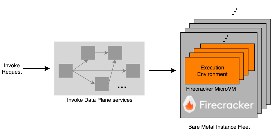


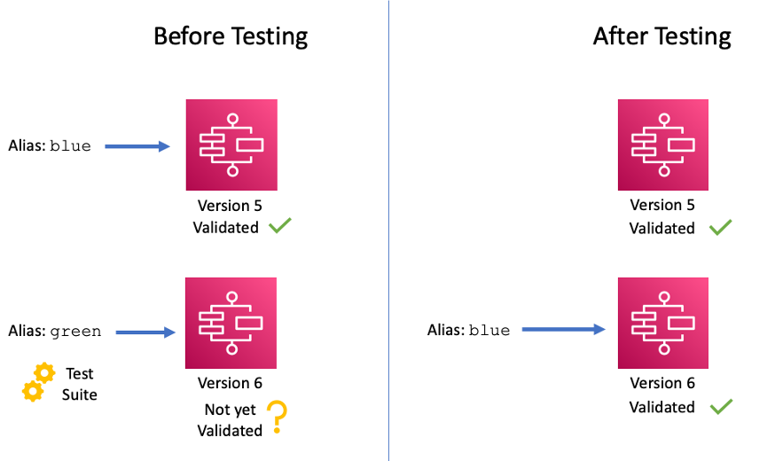


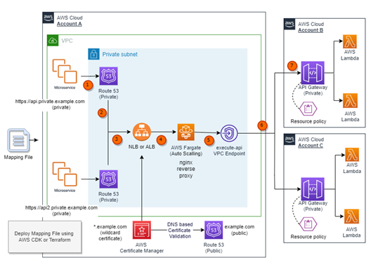
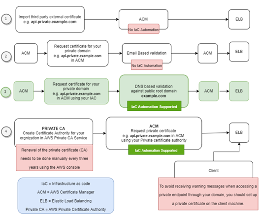

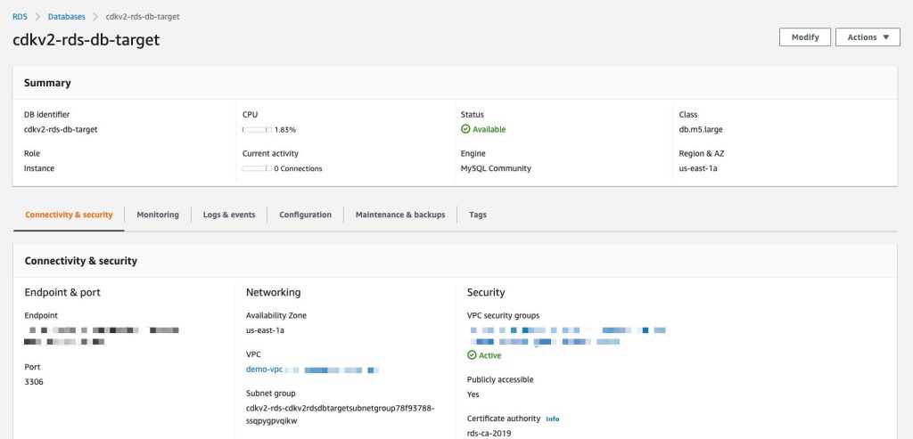
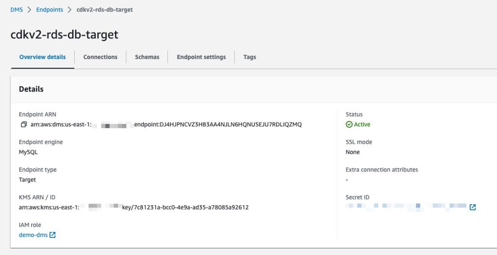

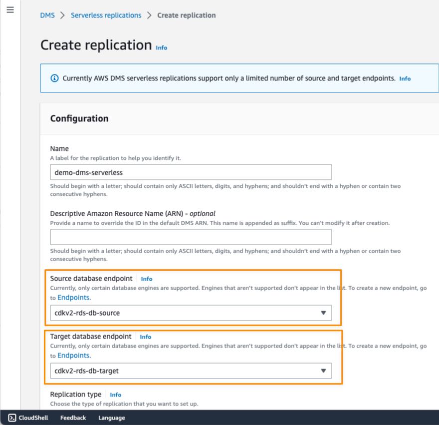
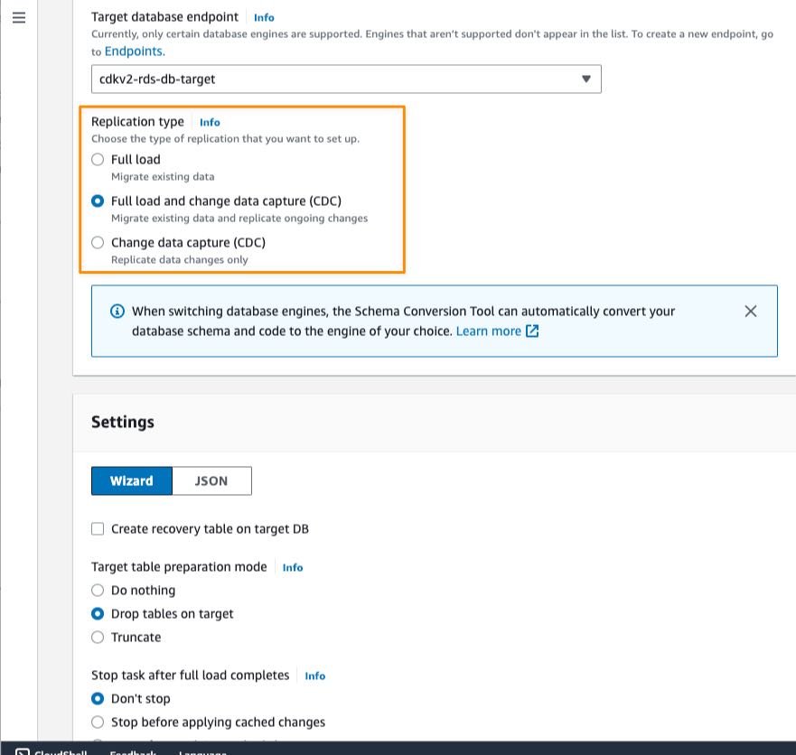
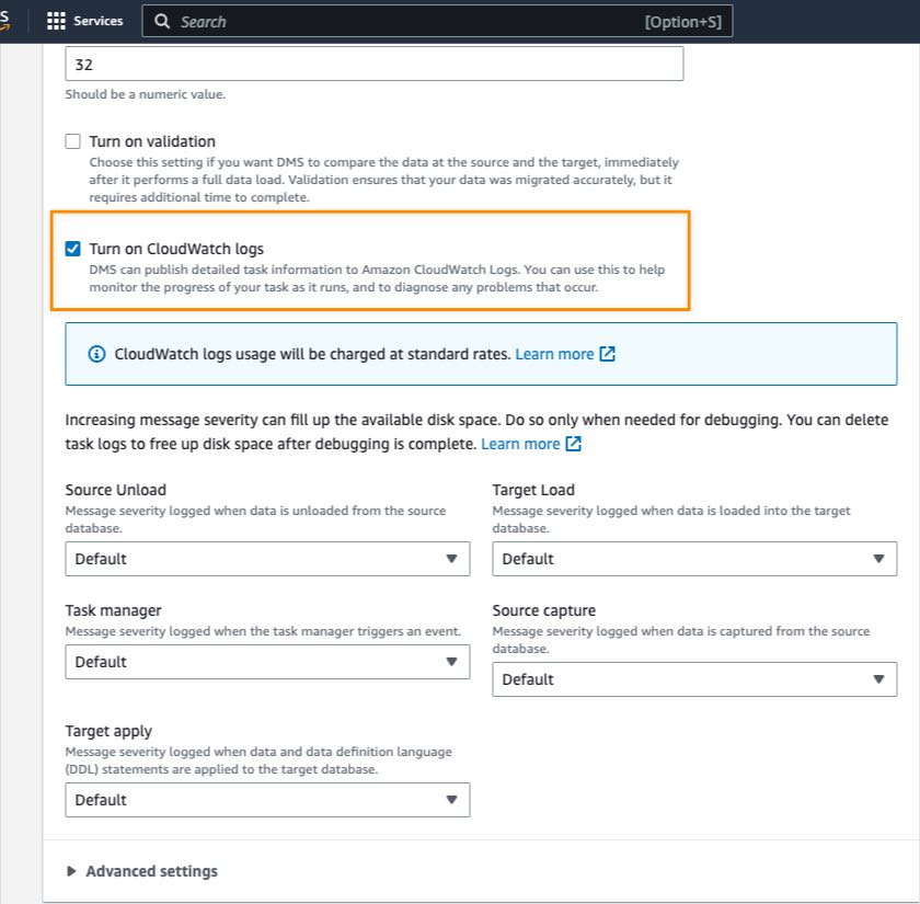
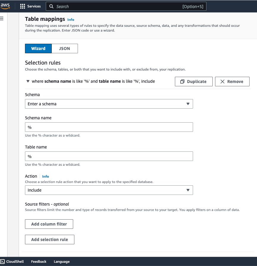
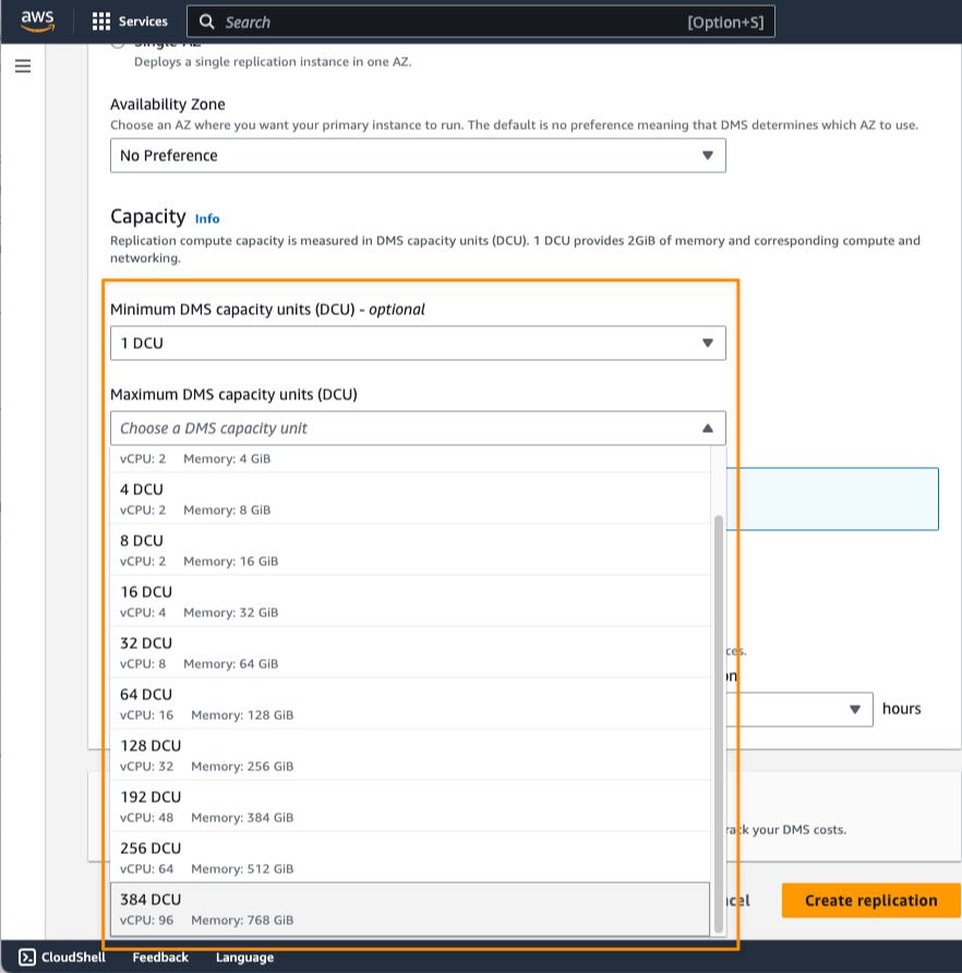


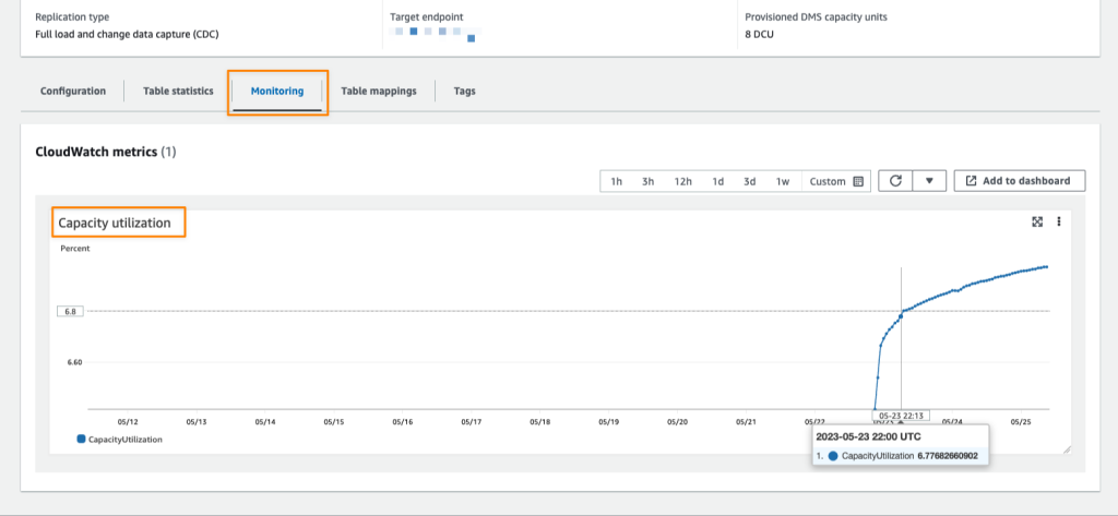
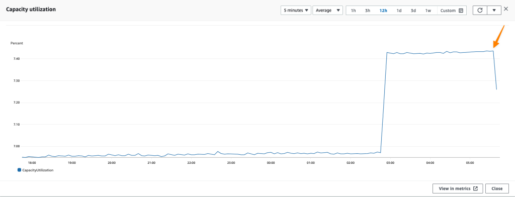
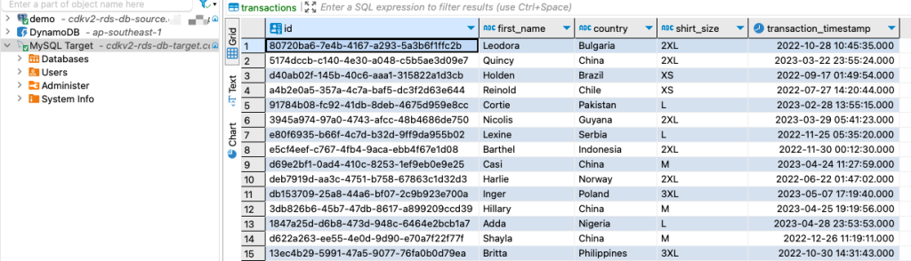

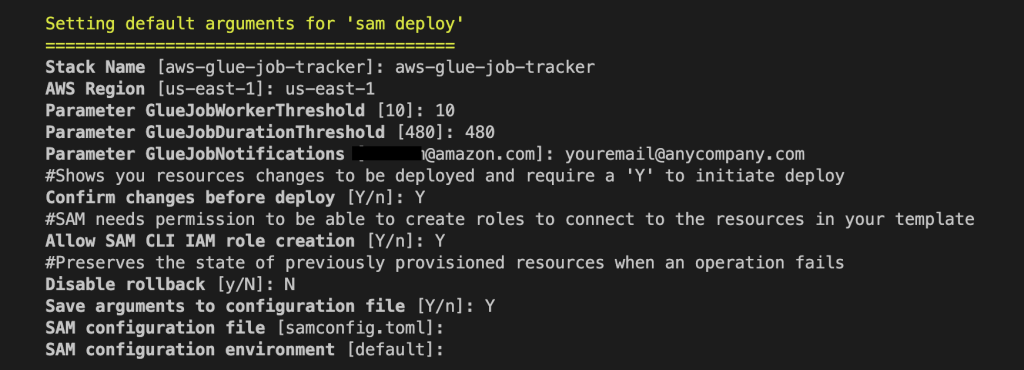

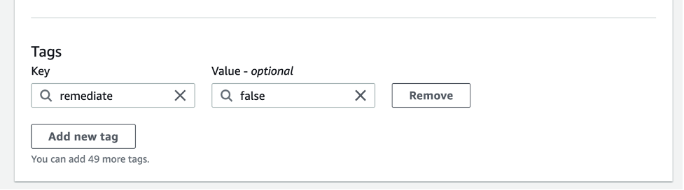
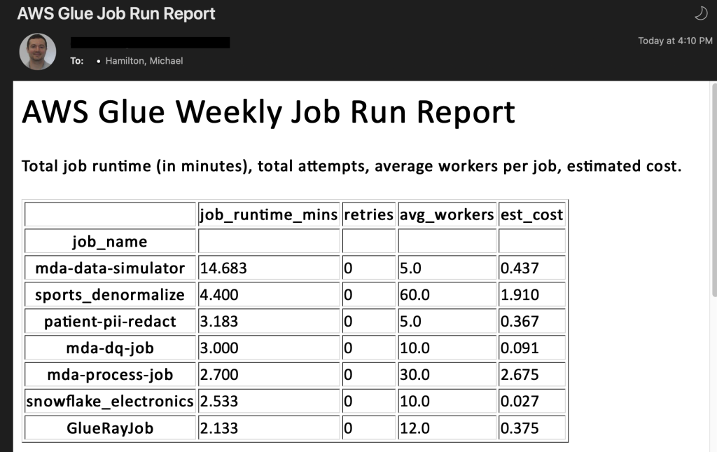
 Michael Hamilton is a Sr Analytics Solutions Architect focusing on helping enterprise customers in the south east modernize and simplify their analytics workloads on AWS. He enjoys mountain biking and spending time with his wife and three children when not working.
 Angus Ferguson is a Solutions Architect at AWS who is passionate about meeting customers across the world, helping them solve their technical challenges. Angus specializes in Data & Analytics with a focus on customers in the financial services industry.