Building Git infrastructure for agent-scale development

Post Syndicated from Brian Celenza original https://github.blog/engineering/architecture-optimization/building-git-infrastructure-for-agent-scale-development/


Every day on GitHub, millions of developers build the products their customers rely on, contribute to open source, and pursue personal projects. GitHub’s architecture has changed steadily over the years to support that work and the growing demands of the developers and organizations who depend on it.

Agentic software development is driving the next architectural shift. With developers and agents working concurrently in repositories that receive millions of commits a day, these workloads demand a different Git architecture. We’re rebuilding GitHub’s Git infrastructure to support them. This post explores the demands shaping that work and the design principles behind it.

Today’s highest-volume workloads show the scale we’re building for. The gap between a typical repository and the busiest ones is wider than most people expect. Here’s a rough picture of the monthly repository activity distribution on GitHub from August 2026:

Repository activity climbs sharply at the far end of the distribution. The busiest repository on GitHub saw roughly a billion requests in August.

Beyond these highest-volume workloads, total Git activity on GitHub is also growing rapidly: between September 2025 and August 2026, it increased to more than 2x its previous level, from 218.2 billion events per month to 473.3 billion.

In September alone, developers and agents made 7.38 billion commits on GitHub, more than five times as many as a year earlier.

The repositories at the top of this curve show what agentic development looks like at its leading edge: large engineering teams running busy CI pipelines alongside growing fleets of agents. Supporting these teams means building Git infrastructure for sustained, concurrent reads and writes at a scale few repositories reach today. We’re investing deeply in Git infrastructure to meet the demands of agentic software development and give teams a foundation built for their most ambitious workloads.

Building for this scale means addressing several architectural challenges:

  • Commit turnaround becomes a bottleneck per agent. An agent in a tight loop commits or checkpoints after nearly every action. Its speed is bounded by how fast a single push completes, so latency that a human would never notice becomes the limiting factor.
  • Write throughput demand is increasing by orders of magnitude. Pushes grew 4.9x year over year, from 0.69 billion to 3.35 billion per month. Thousands of agents working on their own branches in one repository produce a sustained write rate that converges on a single point in our architecture.
  • Merges contend on one reference. Trunk-based development, release trains, and merge queues funnel all that work onto a single ref that has to absorb every merge. Pull request merges on GitHub grew to nearly 4x their volume a year ago.
  • Each push multiplies into thousands of reads. For example, CI and code scanning clone or fetch the same branch tip thousands of times per minute, and that fan-out has to be cheap. GitHub Actions alone ran 3.26 billion times in September, more than 4x as many as a year ago.
  • Operations on a repository must continue to be fast. To keep them fast, we continually compact repository data and clean up objects that are no longer needed. Every new write adds to that work, and the cost compounds as volume climbs.

This is why fast clones only solve part of the problem. Reads are relatively easy to scale: add caches, add replicas, and serve the same bytes to more clients. Scaling reads is essential, but these workloads require more than that. Writes are way harder. Every push has to be stored durably and made visible consistently before the next agent or CI job can build on it.

Where today’s architecture meets new demands

The current architecture has served developers well for years. Every repository is stored by Spokes, which keeps a full copy on the local disks of several fileservers, five by default. Those fast local disks let Git operations read native repository data with low latency, and the extra copies provide redundancy while spreading reads across fileservers. When a push updates a reference, a three-phase commit protocol uses a quorum to ensure that CI, the web UI, and API clients see a consistent repository state. That pairing serves a billion repositories today.

However, the mechanism we use for durability is the same one we use for scale. The copies on disk are the source of truth, so adding read capacity means adding another durable replica. Every replica participates in every write, so a push is only as fast as the slowest replica in its set. The net effect: adding replicas to absorb read load makes writes slower.

For most repositories, this tradeoff works well. At the highest activity levels, it becomes a ceiling: adding read replicas adds overhead to writes, losing a replica reduces read capacity, and losing quorum stops writes entirely. To meet agent-first demands, we need to separate durability from scale without losing what teams rely on today.

Built for the busiest, better for everyone

We’re rebuilding the infrastructure while GitHub keeps running. There’s no maintenance window where the world’s code stops moving, and no version of this work where we ask people to change how they build software while we do it.

We’re building for the most demanding workloads on GitHub: an enterprise shipping under strict regulatory requirements, a team landing a change across a repo that builds an operating system, and an organization running thousands of agents against a single codebase. Engineering for that scale raises the floor for everyone. The maintainer reviewing contributions from volunteers across time zones and the student opening their first pull request get the same faster, more resilient foundation.

The new architecture also must preserve the controls teams already operate on. A maintainer needs branch protections and required reviews so an unreviewed change never reaches the default branch. A security team needs audit logs and repository visibility to investigate a suspicious access event. An on-call engineer needs dependable automation and enough observability to understand why a deployment failed.

For the platform to keep serving everyone here while it scales for the busiest workloads, these are our guiding principles:

  • Build on the workflows developers already trust. Teams rely on workflows like branching, review, merge, and history to build, ship, and govern software at scale. Our new infrastructure is designed to support those same workflows at much higher volumes of activity.
  • Put reliability first. We measure every decision against the reliability that developers and organizations require. Confidence in the platform is what lets an engineering organization build automation, ship on a schedule, meet compliance obligations, and understand the software it produces. This work will meaningfully improve throughput and scale, and those gains extend a foundation of trust that’s already there.
  • Keep people in control of their code. If the system isn’t helping the people and organizations who use it, and isn’t under their control, it isn’t worth building. As agents take on more of the work, the people who own the code can still review, understand, and approve it.

The approach

We are building a new GitHub architecture that can scale much more effectively. Our approach centers around core distributed systems design tenets, applied to the concurrency and scale of agentic software development. Our goal is to continue the forward momentum for open-source communities and enterprises around the world who have built their projects with Git and GitHub, while preserving and adapting the features and controls around it to meet the new needs of the agentic era.

Minimize coordination

A repository that receives many pushes must accept and publish updates quickly. Coordination is valuable when it protects correctness, but too much of it limits write throughput and can turn a busy repository into a bottleneck. Our current architecture is tightly coupled in places it doesn’t need to be, which limits our ability to scale across reads and writes without tough trade-offs. We’re redesigning the system to preserve the coordination that Git semantics require and let everything else proceed independently.

  • Coordinate only what needs agreement. The part of a push that truly needs agreement is the reference update itself. Storing the underlying objects, validating object connectivity, and secret scanning are much more work, but most of it can happen in parallel to other writes. That shrinks the critical path of a push to the small step that needs coordination, so the rest of the work no longer delays the acknowledgment.
  • Move maintenance off the serving path. Compaction and garbage collection are among the heaviest work a repository does, and today they run on the same hosts that answer live Git requests. In the new architecture, separate workers handle maintenance directly against durable storage. A busy repository can be optimized continuously in the background without slowing pushes and fetches.

Decouple storage from compute

Today, complete repository copies on local disks serve both as durable storage and as the layer that answers Git requests. Separating the two lets us scale each one independently.

  • Scale reads without adding durable copies. In the new architecture, read capacity comes from lightweight workers that cache data to serve requests. The authoritative copy of the repository lives in a durable storage layer underneath. That way, the platform can absorb large read spikes from CI fan-out, agent fleets, and large clones without adding work to every push.
  • Let each layer do one job. Authoritative repository data lives in Azure Blob Storage, which already provides durability and replication at Azure scale. The compute layer is optimized for throughput at the lowest latency.
  • Recover faster from failures. When storage and compute are coupled, losing a host reduces both capacity and durability, and recovery means rebuilding a full repository copy. When they’re separate, losing a compute worker is closer to a cache miss: a replacement worker can start serving requests right away and fill its cache from durable storage as traffic arrives.
  • Match capacity to demand. Compute workers can be added or removed as traffic changes instead of provisioning for peak load in advance. A repository going through a burst of activity, like a release or a new agent fleet coming online, can get extra capacity for the burst. Once it passes, that capacity goes away.

Together, these tenets allow us to support higher throughput and more concurrent work without abandoning the reliability and controls that our users need.

What comes next

We’re building an architecture designed to provide the highest throughput and reliability available. Reads and writes scale independently, and the system recovers gracefully from failures. In internal benchmarks, it has delivered up to 35 times higher write throughput, with read capacity that scales on its own to meet demand.

As automated development increases the frequency and concurrency of software change, GitHub will evolve its foundations without trading away the governance and control that teams rely on. We’re already putting that foundation in place. In the next post in this series, we’ll dive deeper into our future architecture and the journey that led us there.

The post Building Git infrastructure for agent-scale development appeared first on The GitHub Blog.
Improving SPIRE security and resiliency with AWS managed services

Post Syndicated from Brendan Paul original https://aws.amazon.com/blogs/security/improving-spire-security-and-resiliency-with-aws-managed-services/

In cloud-centered environments, establishing trust between workloads is fundamental to securing machine-to-machine communication. Traditional approaches such as API keys, shared secrets, and static service account credentials weren’t designed for the scale and ephemeral nature of cloud workloads. This drives an organizational need to shift from long-term, static credentials to short-lived cryptographic workload identities. Organizations are turning to SPIFFE (Secure Production Identity Framework for Everyone) as a core component of their workload identity strategy. SPIFFE is a set of open source standards for securely identifying software systems in dynamic and heterogeneous environments. Using SPIFFE can help address what’s known as the bottom turtle problem: the circular dependency where protecting one credential requires yet another credential.

SPIRE (the SPIFFE Runtime Environment) is an open source implementation of SPIFFE. Customers can use it to quickly experiment with the framework. However, there are operational and security considerations when deploying SPIRE in production, such as:

  • Where cryptographic signing keys for workload identities are managed
  • How to ensure availability and resiliency of the workload identity registry
  • How the SPIRE Certificate Authority integrates into the existing enterprise PKI
  • How workloads without direct connectivity to the SPIRE server validate identities
  • How workload identities are delivered to serverless environments
  • How fine-grained authorization based on SPIFFE IDs is enforced

In this post, we show you how to address each of these considerations by offloading SPIRE core functionality to AWS managed services. This post is accompanied by a Github Repository that guides you through the deployment of the reference architecture.

To learn the core concepts the SPIFFE framework, take a moment to familiarize yourself with the SPIFFE documentation.

SPIRE background

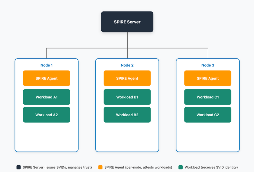
A SPIRE deployment is comprised of at least one SPIRE Server, at least one SPIRE Agent, and at least one workload.

Figure 1: SPIRE high-level architecture

Figure 1: SPIRE high-level architecture

The SPIRE Server is deployed on a central control plane instance (or instances) and manages identity issuance and stores workload identity registrations. The SPIRE server handles five key functions:

  • RegistrationAPI: Create, update, and delete registration entries that define which workloads are entitled to specific SPIFFE IDs based on selectors (for example, Kubernetes namespace, Unix UID).
  • DataStore: The SPIRE server uses a data store to keep track of the workload identity registration entries and the status of the SVIDs it has issued.
  • KeyManager: Controls how the server manages private keys used to sign X.509-SVIDs and JWT-SVIDs.
  • BundlePublisher: Publishes the local trust bundle to a store. The trust bundle is an object containing a trust domain’s cryptographic keys
  • UpstreamAuthority: Dictates which root certificate authority is used to sign the SPIRE certificate authority (CA) certificate

The SPIRE Agent is distributed across your workloads, whether they run on Amazon Elastic Compute Cloud (Amazon EC2) instances, Amazon Elastic Container Service (Amazon ECS) containers, or Amazon Elastic Kubernetes Service (Amazon EKS) Pods. The SPIRE Agent handles:

  • WorkloadAPI: Exposes the workload API to workloads, which enable workloads to retrieve their SVIDs and trust bundles from the SPIRE server.
  • NodeAttestation: SPIRE requires that each agent attest and verify itself.
  • WorkloadAttestation: The SPIRE agent collects workload metadata to determine its identity.
  • SVIDStore: The SPIRE Agent also stores SVIDs in other destinations, such as AWS Secrets Manager or HashiCorp Vault making them available for workloads running in serverless environments.

After the server and agent are deployed, applications retrieve short-lived SPIFFE Verifiable Identity Documents (X.509 Certificates or JSON Web Tokens (JWTs)) using the workload API.

How to use AWS managed services for core SPIRE functions

In the following sections, we dive deeper into what each of these SPIRE functions does and the advantages of using each AWS service for the function.

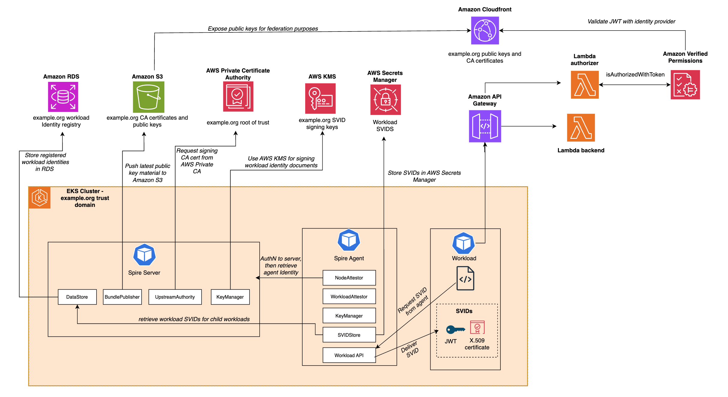
Figure 2: SPIFFE architecture using AWS managed services

Figure 2: SPIFFE architecture using AWS managed services

To deploy the infrastructure required to follow along with this post, follow the deployment process in the Github Repository.

Note: For each managed service, there’s a parameter in the source AWS CloudFormation templates that you can use to specify whether to provision the resource. For example, if you already have an AWS Private Certificate Authority (AWS Private CA) certificate authority deployed in your environment, you can use that for your SPIRE implementation and avoid provisioning a new certificate authority.

SPIRE Key Manager using AWS KMS

The SPIRE Key Manager controls the cryptographic keys that are used to sign SPIFFE Verifiable Identity Documents (SVIDs), which are either X.509 certificates or JWTs.

By using SPIRE, you can configure the cryptographic keys to be either stored in memory or on disk, or to use a plugin where external keys are used for signing SVIDs.

By using the AWS KMS plugin for SPIRE, you bring the security benefits of AWS KMS to your SPIRE implementation.

  • HSMs: AWS KMS uses hardware security modules (HSMs) that have been validated under FIPS 140-3 Level 2
  • Key protection: Your plaintext AWS KMS keys don’t leave the HSMs, aren’t written to disk, and are only used in the volatile memory of the HSMs for the time needed to perform your requested cryptographic operation
  • Comprehensive auditing: Each request to use the keys for signing must be authenticated using Signature Version 4 (SigV4) and is audited and logged in AWS CloudTrail
  • Fine-grained access control: Use AWS KMS Key Policies to restrict access to your signing keys

This configuration block indicates to SPIRE that AWS KMS keys are used to sign our SVIDs:

KeyManager "aws_kms" {
plugin_data {
region = "<your-region>"
key_identifier_file = "./key_metadata"
}
}

This code block exists in the SPIRE server configuration deployed in the Github repository.

SPIRE datastore using Amazon Aurora

The SPIRE server uses a data store to keep track of the workload identity registration entries as well as the status of the SVIDs it has issued. By default, the datastore lives as an SQLite database in memory. However, you can configure the SPIRE server to use Amazon Aurora. By doing this, you can decouple the database from the server and offload the operational overhead of managing the datastore to AWS.

Benefits:

  • High availability: Automatic failover and multi-Availability Zone deployments
  • Automated backups: Point-in-time recovery and automated backup retention
  • Scalability: Scale compute and storage independently
  • Security: Encryption at rest and in transit, with AWS Identity and Access Management (IAM)
  • Monitoring: Built-in performance insights and enhanced monitoring
  • Reduced operational burden: Automated patching, maintenance, and updates

To do this, the CloudFormation stack provisions:

  • An Aurora PostgreSQL Cluster
  • A database user with the capability to authenticate through AWS IAM
  • Network connectivity between your SPIRE Server and the database

After the sample finishes deployment, the configuration in the SPIRE server is changed from the default:

DataStore "sql" {

plugin_data {

database_type = "sqlite3"

connection_string = "/opt/spire/data/server/datastore.sqlite3"

}

}

To:

DataStore "sql" {

plugin_data {

database_type "aws_postgres" {

region = "<region>"

}

connection_string = "dbname=<dbname> user=spiffe host=<your_db_endpoint> port=<your_port>"

}

}

For more information, see Datastore SQL Plugin.

SPIRE certificate authority using AWS Private Certificate Authority

The SPIRE Server issues SVIDs to SPIRE agents and workloads. Given that these SVIDs are X.509 certificates, the SPIRE server needs to act as a certificate authority. In the default configuration of SPIRE, the server generates a self-signed certificate that it will use as the root CA certificate. In production scenarios, organizations often use their existing AWS Private CA certificate authority hierarchy.

Using the AWS Private CA plugin for SPIRE, you configure the SPIRE CA to act as an issuing certificate authority that chains to your existing root CA. This delivers three benefits for your SPIRE implementation:

  • HSM-backed root of trust: The root of trust of your CA hierarchy is backed by fully managed, FIPS 140-2 Level 3 validated hardware security modules
  • Non-exportable private keys: The private keys for the root CA can’t be exported
  • Fully Managed Certificate Revocation Lists and OCSP endpoint: In case the issuing CA certificate needs to be revoked

Note: If the SPIRE CA certificate will be signed by an issuing CA, you need to ensure that the path length of that CA is at least 1. The sample code provisions a root CA, so this isn’t an issue if you’re following the sample code.

After the sample deployment is complete, the configuration of the SPIRE server configuration includes the UpstreamAuthority plugin to use your AWS Private CA certificate authority as the root of trust.

UpstreamAuthority "aws_pca" {

plugin_data {

region = "<aws_region>"

certificate_authority_arn = "<your_pca_arn>"

ca_signing_template_arn = "arn:aws:acm-pca:::template/SubordinateCACertificate_PathLen0/V1"

}

}

For more information, see the AWS Private CA upstream authority plugin documentation.

SPIRE bundle publisher using Amazon S3

In SPIFFE, trust bundles are sets of public keys that are used by destination workloads to verify the identity of source workloads. These bundles contain the root certificates and public keys used to sign JWT SVIDs.

The SPIRE Server supports exposing an endpoint containing this trust bundle or publishing the bundle to Amazon Simple Storage Service (Amazon S3).

By publishing the bundle to Amazon S3, you can:

  • Decouple: Decouple bundle access from the SPIRE server availability
  • Continuous validation: Allow destination workloads to continually validate source workload identities without requiring network access to the SPIRE server
  • Global distribution: Distribute the trust bundle using Amazon CloudFront, improving performance through the CloudFront global edge network with over 750 Points of Presence
  • Reduced load: Offload trust bundle retrieval traffic from the SPIRE server
  • Version control: Maintain historical versions of trust bundles with S3 versioning

The following is a sample configuration for this plugin:

BundlePublisher "aws_s3" {

plugin_data {

region = "<your_bucket_region>"

bucket = "<your_bucket_name>"

object_key = "<your_bundle_name"

format = "spiffe"

}

}

For more information, see S3 Bundle Publisher Plugin Reference.

SPIRE Agent SVID store using Secrets Manager

In a typical SPIRE implementation, SVIDs are retrieved from the workload API using the SPIRE agent by workloads. In serverless or container cases, it isn’t feasible or possible to run the SPIRE agent, especially in workloads running on AWS Lambda or an AI agent running in Amazon Bedrock AgentCore Runtime. In these scenarios, use the SVID store plugin to push the SVID to Secrets Manager.

In this scenario, you still need a SPIRE agent running on a node that performs node attestation with the SPIRE server and delivers the SVID to a secrets store. One of the available secrets store plugins is the AWS Secrets Manager SVIDStore Plugin.

Benefits:

  • Encryption at rest: Secrets are encrypted by default using AWS managed or customer-managed AWS KMS keys
  • Broad integration: Integrations with multiple compute types, including AWS Secrets Manager Lambda Extension, Amazon ECS, Amazon EMR, and 52 other AWS services
  • Client-side caching: Secrets Manager provides client-side caching libraries to improve performance and reduce API calls
  • Multi-region replication: Built-in multi-Region replication functionality for workloads with multi-region requirements
  • Fine-grained access control: Use resource policies to control which workloads access which SVIDs
  • Audit trail: All secret access is logged in CloudTrail

This plugin is configured in the agent, as opposed to the SPIRE server. A reference for the specific permissions required are in the plugin Github repository. In the sample code, see the configuration in the following agent.conf file:

SVIDStore "aws_secretsmanager" {

plugin_data {

region = "<your_region>"

}

}

When you need to specify a given workload’s SVID to be pushed to Secrets Manager, you add the storeSVID and selector parameters when you create the entry in the workload registry. If you’re managing your SPIRE server in Kubernetes, the appropriate command looks like:

kubectl exec -n spire spire-server-<postfix>-- \

/opt/spire/bin/spire-server entry create \

-spiffeID spiffe://example.org/<workload_name> \

-parentID spiffe://example.org/ns/spire/sa/spire-agent \

-selector aws_secretsmanager:secretname:<workload_name> \

-storeSVID

Fine-grained access control using Verified Permissions

Up to this point, all the managed services we’ve talked about have been used for creating and distributing SVIDs and trust bundles to workloads. However, a key advantage of using a framework such as SPIFFE is that it allows resource owners to protect resources with fine-grained access control. One managed service that helps you do that in the context of SPIFFE and SPIRE implementations is Amazon Verified Permissions.

Verified Permissions is a scalable, fine-grained permissions management and authorization service that helps you build secure applications. You can use it to:

  • Define declarative policies: Use Cedar policy language, which provides human-readable, declarative access control rules
  • Centralize policy management: Separate authorization logic from application code
  • Take advantage of the straightforward policy authoring, formal verification capabilities, and performance benefits of Cedar
  • Make real-time decisions: Evaluate authorization requests in real-time based on multiple factors including user identity, workload identity (SPIFFE ID), resource attributes, and contextual information
  • Integrate with identity providers: Support for OpenID Connect (OIDC) providers, enabling validation of JWT tokens including JWT-SVIDs

With Verified Permissions, you authenticate SPIRE issued SVIDs using the public keys associated with your trust domain, and deploy fine-grained authorization policies protecting your resources. To use Verified Permissions, you need a policy store, an identity source, and authorization policies.

The github sample creates a policy store on your behalf and sets up the necessary infrastructure to have SPIRE serve as an identity source for your policy store.

You will need policies to enforce fine grained authorization. The following sample policy forbids a specific workload from taking any action:

forbid(

principal,

action,

resource

)

when {

context has sub &&

context.sub like "spiffe://example.org/forbidden-workload/*"

};

Or conversely allows a specific workload to take actions:

permit(

principal,

action,

resource

)

when {

context has sub &&

context.sub like "spiffe://example.org/allowed-workload/*"

};

Experiment with these policies as you build on top of your SPIRE infrastructure.

Conclusion

This post demonstrates how organizations enhance their SPIRE deployments on AWS by replacing default implementations with AWS managed services. We showed you integrations with AWS KMS for SVID signing, Amazon RDS Aurora for managed datastore operations, AWS Private Certificate Authority for root of trust, Amazon S3 and CloudFront for global trust bundle distribution, AWS Secrets Manager for SVID storage, and Amazon Verified Permissions for fine-grained authorization. By adopting these integrations, organizations can improve security posture, reduce operational complexity, and enhance resiliency.

If you’re interested in learning SPIFFE on AWS, check out our SPIRE on AWS github sample or the SPIFFE and SPIRE on AWS Workshop for hands-on learning.

If you have feedback about this post, submit comments in the Comments section below.


Brendan Paul

Brendan is a Security Services SA Manager at AWS and has been at AWS for more than 7 years. He spends most of his time at work helping customers solve problems in the data protection and workload identity domains. Outside of work, he’s pursuing his master’s degree in data science from UC Berkeley.

Meg Peddada

Meg Peddada

Meg is a Principal FSI Security Solutions architect specializing in security, risk, and compliance. Her expertise spans governance, security automations, threat management, and architecture. In her spare time, she loves playing volleyball, arts and crafts, and finding new brunch experiences.

The keys to the Internet change on October 11. Are you ready?

Post Syndicated from Sebastiaan Neuteboom original https://blog.cloudflare.com/root-ksk-2024-rollover/

On October 11, 2026, the DNS root is scheduled to change its key-signing key (KSK) for only the second time ever. This key anchors DNSSEC’s chain of trust, which lets DNS resolvers authenticate answers using cryptographic signatures. The change is called a KSK rollover. Validating resolvers need to trust the new key before the switch, as otherwise healthy websites could become unreachable.

When we wrote about the first root KSK rollover in 2018, we had seen resolvers lose their learned trust in the new key during software upgrades or moves between machines. Publishing the key well in advance was only part of the job. We also needed to know whether resolvers had retained it, and we couldn’t give users a practical way to check.

Most website operators do not need to make any changes for this rollover. If you run a DNSSEC-validating resolver, check that it trusts the new root key, KSK-2024, and follow your software vendor’s instructions to update its trust anchors if the key is missing. If you use Cloudflare for your domain's DNS or rely on 1.1.1.1 and Gateway DNS, you do not need to take any action — our systems already trust KSK-2024.

To check ahead of time, visit our rollover readiness test. It asks the resolver your browser uses whether it trusts the new key. The test uses RFC 8509: A Root Key Trust Anchor Sentinel for DNSSEC, which we’ve implemented in 1.1.1.1 ahead of the rollover.

Where DNSSEC trust begins

A DNS resolver looks up the addresses of websites and other services for your device. DNSSEC lets it check digital signatures on DNS records to verify that they are authentic and have not been changed. The resolver also needs to check that the public keys used to verify those signatures belong to the right domains.

For cloudflare.com, this follows a chain of trust from the DNS root to .com, then to cloudflare.com. Each parent publishes a Delegation Signer (DS) record containing a fingerprint of its child’s public key. For example, .com publishes the DS record for cloudflare.com, allowing the resolver to check that domain’s key.

That chain needs a starting point. The root, however, has no parent to confirm which keys belong to it. Instead, a resolver checking DNSSEC starts with a root public key, or its fingerprint, that it already trusts. This is called a trust anchor.

The root’s signing keys have two different jobs. The zone-signing key (ZSK) signs the root’s DNS records, including the DS records for top-level domains such as .com. The key-signing key (KSK) signs the list of public keys published by the root, called the DNSKEY record set. The resolver uses its trusted KSK to verify that list, then uses the ZSK from the list to verify the root’s other records.

The diagram below shows the arrangement for a typical signed zone. For the root, trust comes from the resolver’s trust anchor rather than a DS record in a parent zone.

Our posts about the .de and the .al rollover failures showed the consequence of failed DNSSEC checks: websites can be working normally but still be unreachable. The root KSK rollover changes the starting point of those checks. If a resolver does not trust the replacement key, its users may be unable to reach websites under any top-level domain.

The new key is KSK-2024, identified by key tag 38696. It will replace KSK-2017, key tag 20326, as the signer of the root’s DNSKEY set. Validating resolvers need to trust the new key before that switch.

How resolvers get the new root key

RFC 5011 lets resolvers learn a new root trust anchor automatically. The root publishes the new KSK alongside the existing one in its DNSKEY set. The existing KSK continues signing that set, so a resolver can use the key it already trusts to verify the records containing the replacement.

Before accepting the new key as a trust anchor, the resolver waits at least 30 days and keeps checking the root’s signed DNSKEY records. The new key must remain in the records it checks during that period. After the wait, the resolver must successfully verify the records containing the new key again before accepting it.

For this rollover, KSK-2024 has been published in the root’s DNSKEY set since January 11, 2025. That gave resolvers with automatic trust-anchor updates time to discover and accept it ahead of the scheduled October 11, 2026 signing change. Each resolver’s waiting period starts when it first sees and verifies the new key.

For our resolver, we added KSK-2024 directly to the software’s built-in trust anchors in July 2024, alongside KSK-2017. A resolver running the updated software therefore has the new anchor available from startup.

We chose this approach because of our experience during preparations for the first rollover. As described in our 2018 post, software upgrades and moves between machines caused some resolvers to lose their learned trust-anchor state. We fixed that by updating the software to include the new anchor by default. Including KSK-2024 in the software likewise avoids depending on each resolver retaining a key it learned automatically.

Even though we added KSK-2024 to our resolver’s built-in trust anchors in July 2024, users of 1.1.1.1 and Gateway DNS had no direct way to check whether the resolver answering their queries trusted the new key.

This time, ask the resolver

RFC 8509 defines the root key trust anchor sentinel, a way to ask a supporting resolver whether it trusts a particular root key. It uses ordinary DNS queries with specially named domains.

Our readiness test website uses this protocol to check for KSK-2024. Two names ask opposite questions: is-ta-38696 asks whether the key is trusted, not-ta-38696 asks whether it is not trusted.

Both names have valid DNSSEC-signed address records. A resolver that supports the sentinel first validates those records, then either returns the response directly or replaces the answer with SERVFAIL, depending on whether it trusts the key.

For a validating resolver with sentinel support, the expected results are:

Query

KSK-2024 is trusted

KSK-2024 is not trusted

is-ta-38696

Returns a valid response

Returns SERVFAIL

not-ta-38696

Returns SERVFAIL

Returns a valid response

For a validating resolver with sentinel support, SERVFAIL for not-ta-38696 is expected when KSK-2024 is trusted. The resolver deliberately rejects the “not trusted” query.

Sentinel labels such as root-key-sentinel-is-ta-38696 can be used under any DNSSEC-signed domain. We use dnstest.dev for our tests. You can run the two queries directly against 1.1.1.1:

The website also checks that an ordinary signed name resolves, that a deliberately invalid DNSSEC name is rejected, and that the resolver responds to a sentinel query for the current root key. These controls help distinguish a meaningful result from a failed lookup or unsupported protocol. If sentinel support cannot be established, the result is inconclusive; it does not mean the new key is missing.

The browser test checks the resolver your browser uses, which may be affected by Secure DNS or a VPN. The dig commands above explicitly query 1.1.1.1. Both provide a snapshot of the resolver path answering those requests.

New key, same algorithm

KSK-2017 and KSK-2024 both use RSA/SHA-256. The rollover replaces the key pair while keeping the same method for creating and verifying signatures.

In our 2018 post, we wrote that a successful rollover would open the door to discussing an algorithm change. Eight years later, the root still uses RSA.

Replacing the key remains useful. It limits how long a single private key stays in use and exercises the process of distributing new trust anchors, updating resolvers, and retiring old keys. As the first rollover showed, those steps can fail even when the cryptography itself works correctly.

The Internet Assigned Numbers Authority (IANA) plans an idealized three-year rollover interval, balancing regular practice against the work and risk of changing the root key too frequently. The gap since 2018 has been longer. The Internet Corporation for Assigned Names and Numbers (ICANN) attributes the delay to pandemic disruption and upgrades to the hardware that protects the private signing keys.

Changing algorithms means resolvers need both a new trust anchor and software that can verify the new signatures. Regular key rollovers let operators test the trust-anchor updates while keeping the algorithm the same.

What comes after October

The October 11 switch changes which KSK signs the root’s DNSKEY set. The rollover continues into 2027, when ICANN plans to revoke KSK-2017, remove it from the root zone, and delete its private key. Stopping a key from signing and removing trust in that key are separate steps.

ICANN has also proposed a future root algorithm rollover to ECDSA P-256. ECDSA produces smaller keys and signatures than the RSA algorithm used today. That proposal is separate from this October’s key replacement, and ECDSA is not a post-quantum algorithm.

1.1.1.1 now validates ML-DSA-44 signatures, which are designed to remain secure against attacks using quantum computers. For DNSSEC’s whole chain of trust to become post-quantum secure, signed domains, their parent zones, and the root must adopt post-quantum cryptography too. At the root, that means introducing a post-quantum KSK and getting resolvers to trust it.

That will require another root key rollover. The rollovers we perform now let operators test how they distribute replacement trust anchors, check that resolvers have accepted them, and retire the old keys. This October’s rollover keeps RSA, but exercises the trust-anchor updates we will need when the root moves to post-quantum cryptography. The sentinel gives us a way to check whether resolvers followed those updates.

We encourage DNS providers and resolver developers to support RFC 8509 trust anchor sentinels. If your resolver does not support them, ask your provider or software vendor to add support. Users should be able to check whether their resolver trusts the next root key before a rollover.

For now, the next deadline is October 11. You can check your resolver’s readiness at https://dnstest.dev/ksk-2024. If you operate a DNSSEC-validating resolver, confirm that it trusts KSK-2024, key tag 38696, and follow ICANN’s guidance and your software vendor’s instructions if the key is missing.

Gigabyte W775-V10-L01 Hands-on Bringing NVIDIA GB300 Deskside

Post Syndicated from Patrick Kennedy original https://www.servethehome.com/gigabyte-w775-v10-l01-hands-on-bringing-nvidia-gb300-deskside/

We test the Gigabyte W775-V10-L01, including getting over 2.2B tokens/ day on the Blackwell Ultra GPU, 800Gbps from the ConnectX-8 SuperNIC, and testing the NVIDIA Grace CPU with the C2C link between it and the GPU

The post Gigabyte W775-V10-L01 Hands-on Bringing NVIDIA GB300 Deskside appeared first on ServeTheHome.

Get started with AWS Lambda SnapStart for container images

Post Syndicated from Sachin Saini original https://aws.amazon.com/blogs/compute/get-started-with-aws-lambda-snapstart-for-container-images/

AWS Lambda recently launched SnapStart for container image functions, reducing startup times from several seconds to as low as sub-second. Customers deploy Lambda functions with container images to align with their organization’s container-based deployment standards, or to package larger dependencies up to 10 GB. However, larger container images can experience startup times of several seconds as Lambda downloads image layers and initializes the runtime and application code. SnapStart addresses this by taking a snapshot of the initialized execution environment during function deployment, caching it, and resuming from it on invocation, instead of initializing from scratch.

In November 2022, Lambda launched SnapStart for Java, reducing startup latency by up to 10x. In November 2024, SnapStart expanded to Python and .NET managed runtimes, reducing cold start latency to as low as sub-second. These launches helped developers achieve faster startup time, but only for .zip file archives. By extending SnapStart support for container image functions, customers can improve startup times for latency-sensitive workloads such as ML inference and interactive APIs.

This post covers how SnapStart for container images works, how to enable it, and best practices and considerations for your workloads.

How SnapStart for container images works

When you deploy a Lambda function, you choose one of two deployment models: a .zip file archive or a container image. With managed runtimes we already support SnapStart for Python, .NET, and Java functions, and now we have extended this capability to container images. When you invoke the deployed function for the first time, or when a burst of traffic arrives, Lambda checks if there is an available execution environment. If none are available, Lambda creates a new one.

For container image functions, this means downloading and extracting image layers, bootstrapping the runtime, and running your initialization code. This process can take several seconds, which users experience as a cold start.

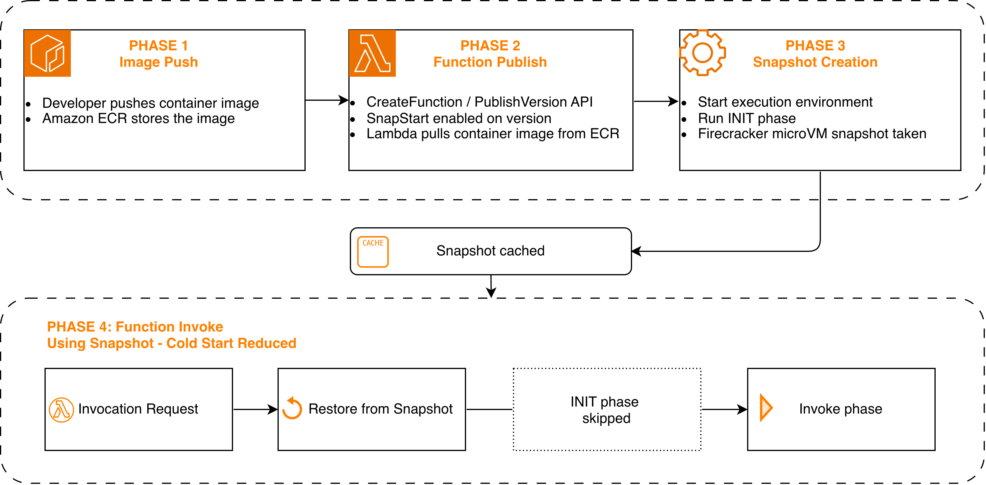
When you enable SnapStart and publish a function version, Lambda proactively creates an execution environment, initializes your function, and then takes a Firecracker microVM snapshot of the full memory and disk state. This snapshot is encrypted and cached for low latency access and remains cached until you delete the corresponding function version.

On invocation, Lambda resumes from the cached snapshot rather than initializing from scratch. With SnapStart, initialization happens once at deployment time rather than on every invocation, replacing the initialization phase with a faster restore phase that speeds up startup time to as low as sub-second.

Diagram of the SnapStart for container images lifecycle, from image push to snapshot restore at invocation

Figure 1: SnapStart for container images lifecycle, from image push to snapshot restore at invocation

Supported base images

For managed runtimes, you provide your code, and Lambda handles the runtime environment. For container image functions, you package your own runtime environment using Lambda-vended base images or your own custom base images. SnapStart for container images supports the following Lambda base images at launch. To learn about supported base images per runtime, see the Lambda SnapStart developer guide.

Runtime Base Image Architecture
Java 11 and later public.ecr.aws/lambda/java:11, :17, :21, :25 x86_64, arm64
Python 3.12 and later public.ecr.aws/lambda/python:3.12, :3.13, :3.14 x86_64, arm64
.NET 8 and later public.ecr.aws/lambda/dotnet:8, :9, :10 x86_64, arm64

Regardless of which base image you use, there is an important consideration to understand before enabling SnapStart. When Lambda restores a function from a snapshot, any state captured during initialization is shared across all execution environments restored from that snapshot. This includes random number generators, unique IDs, cached credentials, and database connections. Your function needs to restore a unique state after each resume to avoid reusing the same random seed or an expired database connection across invocations. For more details on these considerations, see SnapStart uniqueness documentation.

To help you restore uniqueness for your application, Lambda provides runtime hooks for managed runtimes that let you run your own code at specific points in the snapshot-and-restore cycle. With SnapStart for container images, we are extending these same hooks to container image functions.

If your function uses one of the preceding Lambda-managed base images, Lambda offers runtime hooks for you to run your code (for example, to restore database connections). Lambda supports these runtime hooks for Java through CRaC, for Python through snapshot_restore_py, and for .NET through SnapshotRestore. To register your own before-snapshot and after-restore hooks for these runtimes, see SnapStart runtime hooks documentation.

If your function uses a base image without native SnapStart support (for example, a Node.js or Ruby base image), a custom Runtime Interface Client, or a custom runtime built on provided.al2023, review the documentation on implementing SnapStart hooks for container image functions and choose one of the following options.

  • Option 1: Implement SnapStart runtime hooks. If you need to run custom logic when your function is snapshotted or restored, implement the /restore/next API in your container image as described in SnapStart runtime hooks documentation.
  • Option 2: Opt in without hooks. If you do not need before-snapshot or after-restore hooks, add the following label to your Dockerfile (LABEL com.amazonaws.lambda.feature.snapstart=”Allow”)

For a reference implementation of SnapStart runtime hooks integration in a custom runtime, refer to the Lambda Rust Runtime repository, including its examples for both event-driven and HTTP functions to see how SnapStart and runtime hooks are implemented.

Getting started

To get started, you can use the AWS Management Console, AWS Command Line Interface (AWS CLI), AWS Software Development Kits (AWS SDKs), AWS CloudFormation, AWS Serverless Application Model (AWS SAM), or AWS Cloud Development Kit (AWS CDK) to activate, update, and delete SnapStart for container images. You can also use the Agent Toolkit for AWS to enable SnapStart as part of your agent-based workflows.

To use SnapStart with a container image function, your function must be deployed with PackageType Image, and the image must be pushed to an Amazon Elastic Container Registry (Amazon ECR) repository in the same AWS Region as your function. The examples in this section use a supported Lambda base image and us-east-1 as the AWS Region. Either set your default region or add –region to each command.

Activating SnapStart on an existing function

If you already have a container image function using a supported base image, activate SnapStart by updating the function configuration and publishing a version:

aws lambda update-function-configuration \
    --function-name my-function \
    --snap-start ApplyOn=PublishedVersions

aws lambda publish-version \
    --function-name my-function

Creating a new function with SnapStart

Create an Amazon ECR repository:

aws ecr create-repository --repository-name my-function-repo

Start with a Dockerfile using a supported base image. Here is an example for Python:

FROM public.ecr.aws/lambda/python:3.12
COPY requirements.txt ${LAMBDA_TASK_ROOT}
RUN pip install -r requirements.txt
COPY lambda_function.py ${LAMBDA_TASK_ROOT}
CMD ["lambda_function.handler"]

Build, push to Amazon ECR, and create the function with SnapStart in a single flow:

# Build the container image locally. --platform pins the CPU architecture
# (must match --architectures on create-function). --provenance=false is
# required because BuildKit otherwise wraps the image in an OCI image index
# (manifest list) to attach a provenance attestation, and Lambda only accepts
# a single image manifest.
docker buildx build --platform linux/amd64 --provenance=false -t my-function-repo:latest .

aws ecr get-login-password | \
docker login --username AWS --password-stdin 111122223333.dkr.ecr.us-east-1.amazonaws.com
docker tag my-function-repo:latest 111122223333.dkr.ecr.us-east-1.amazonaws.com/my-function-repo:latest
docker push 111122223333.dkr.ecr.us-east-1.amazonaws.com/my-function-repo:latest

aws lambda create-function \
    --function-name my-function \
    --package-type Image \
    --code ImageUri=111122223333.dkr.ecr.us-east-1.amazonaws.com/my-function-repo:latest \
    --role arn:aws:iam::111122223333:role/lambda-execution-role \
    --architectures x86_64 \
    --snap-start ApplyOn=PublishedVersions

# Once the function is active, publish the version
aws lambda publish-version \
    --function-name my-function

Verifying SnapStart is active

After publishing, check the function version configuration:

aws lambda get-function-configuration \
    --function-name my-function:1

When SnapStart is active, the response shows:

{
    "SnapStart": {
        "ApplyOn": "PublishedVersions",
        "OptimizationStatus": "On"
    },
    "State": "Active"
}

Once the state is Active, invoke the published version:

aws lambda invoke \
    --function-name my-function:1 \
    --cli-binary-format raw-in-base64-out \
    --payload '{"key": "value"}' \
    response.json

Note that SnapStart applies only to published versions, not $LATEST. You must invoke a specific version number to use SnapStart.

Best practices and considerations

As SnapStart resumes your function from a point-in-time snapshot, here are some best practices to consider for resources initialized at snapshot time that may become stale when your function resumes, such as network connections, credentials, and unique IDs.

  • Performance tuning: Preload dependencies and initialize resources in your init code rather than the handler. This moves heavy setup into the snapshot, where it’s captured once and reused across restores. For guidance on optimizing function startup latency, see the performance tuning section of the Lambda developer guide.
  • Network connections: Since snapshots can persist over an extended period, connections established during initialization may no longer be valid after restore. Network connections established through an AWS SDK resume automatically. For connections your code manages directly, such as database connections, use after-restore hooks to re-establish them as described in the networking best practices section of the Lambda developer guide.
  • Uniqueness: Avoid generating unique IDs, secrets, or random values during initialization, because these are shared across all execution environments restored from the same snapshot. Instead, generate them in the function handler or use after-restore hooks. Software that always gets random numbers from the operating system (for example, from /dev/random or /dev/urandom) does not need any updates to maintain randomness. Lambda always reseeds /dev/random and /dev/urandom when restoring a snapshot, so random numbers are not repeated even when multiple execution environments resume from the same snapshot. For more details on managing unique state across restores, see the handling uniqueness documentation for Lambda SnapStart.
  • Ephemeral data: Cached credentials, timestamps, or other time-sensitive data captured during initialization may be stale by the time your function resumes from a snapshot. Use after-restore hooks to verify freshness and refresh any expired state before processing requests.
  • Monitoring: Amazon CloudWatch logs include a RESTORE_REPORT line showing the time spent restoring the snapshot. The REPORT line includes Restore Duration, Billed Restore Duration, Duration, and Billed Duration. Note that InitDuration does not appear for SnapStart invocations because the function resumes from a snapshot rather than initializing. You can also use AWS X-Ray active tracing to capture real-time telemetry for extensions through the Telemetry API, and measure end-to-end latency with Amazon API Gateway and Lambda function URL metrics. To learn more about available monitoring options, visit the Lambda documentation on monitoring for SnapStart.

Limitations: Provisioned concurrency, Amazon Elastic File System (Amazon EFS), Amazon Simple Storage Service (Amazon S3) Files and ephemeral storage greater than 512 MB are not supported with SnapStart. Maximum container image size remains 10 GB. If you need any of the currently unsupported features, please reach out to us on the Lambda Roadmap GitHub page.

Pricing and availability

SnapStart for container images uses the same pricing dimensions as SnapStart for Python 3.12+ and .NET 8+. You pay for the cost of caching a snapshot per function version that you publish with SnapStart enabled, and the cost of restore each time a function is restored from a snapshot. To reduce your caching costs, delete unused function versions. Refer to the Lambda pricing page for more details.

Lambda SnapStart for container images is available in all commercial AWS Regions except Asia Pacific (New Zealand) and Asia Pacific (Taipei). For the latest list of supported Regions, see the Lambda SnapStart supported regions.

Cleanup

To avoid ongoing charges for the resources created in this walkthrough, delete them when you are done. Deleting a Lambda function version removes the associated cached snapshot and stops any related snapshot caching charges.

Delete the Lambda function. This removes all published versions and their cached snapshots:

aws lambda delete-function \
    --function-name my-function

Delete the container image and the Amazon ECR repository:

aws ecr delete-repository \
    --repository-name my-function-repo \
    --force

If you created an IAM execution role only for this walkthrough, delete it as well. For details, see deleting an IAM role.

Conclusion

In this post, we described how Lambda SnapStart for container images reduces cold start latency by snapshotting the initialized execution environment and resuming from it on subsequent invocations. We covered how SnapStart works, how to get started based on your base image type, best practices and considerations, and pricing and availability. We look forward to hearing from you about the future capabilities you need for SnapStart, on our Lambda Roadmap GitHub page.

Try SnapStart on your container image functions today. To learn more, visit the Lambda SnapStart documentation. For more serverless learning resources, visit Serverless Land.


About the authors

Rakesh Hemrajani

Rakesh Hemrajani

Rakesh is a Software Development Manager at AWS.

Prerna Choudhary

Prerna Choudhary

Prerna is a Senior Product Manager, Technical at AWS.

Sachin Saini

Sachin Saini

Sachin is a Senior Solutions Architect at AWS.

Monitoring MWAA-orchestrated ETL pipelines with Amazon OpenSearch Service

Post Syndicated from Anupa Bhattacharyya original https://aws.amazon.com/blogs/big-data/monitoring-mwaa-orchestrated-etl-pipelines-with-amazon-opensearch-service/

When your MWAA-orchestrated extract, transform, and load (ETL) pipeline spans multiple AWS services, troubleshooting a failure becomes a scavenger hunt. AWS Glue jobs transform data, custom scripts run on Amazon Elastic Compute Cloud (Amazon EC2), and directed acyclic graphs (DAGs) in Amazon Managed Workflows for Apache Airflow (Amazon MWAA) coordinate the workflow, but each service writes logs to its own Amazon CloudWatch log group. When something breaks at 2 AM, your team spends valuable time locating the right log stream before they can even begin diagnosing the root cause.

These observability challenges aren’t unique to any one team. DevOps engineers routinely juggle multiple tools and must analyze numerous logs to identify and resolve an issue. Every pivot between tools or logs costs minutes during an outage and directly inflates mean time to resolution. Interpreting logs is another challenge. Even when engineers locate the right log stream, parsing the output requires deep familiarity with each service’s logging conventions. A single failed task can scatter relevant context across dozens of verbose, interleaved log entries that obscure the root cause rather than reveal it.

This solution helps you remediate errors in an analytics pipeline by using an AI agent to speed up root cause identification, interpret relevant logs, and recommend how to resolve the issue. In this post, you learn how to implement this analytics observability solution. The target audience is data engineers, DevOps engineers, and cloud engineers.

You deploy a set of provided AWS CloudFormation templates and an Amazon SageMaker AI notebook to implement a sample architecture and create a set of demo ETL jobs orchestrated by Amazon MWAA. The CloudFormation templates deploy the architectural components, and the SageMaker AI notebook contains code to configure the components and interact with the MCP server.

Solution overview

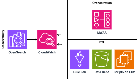
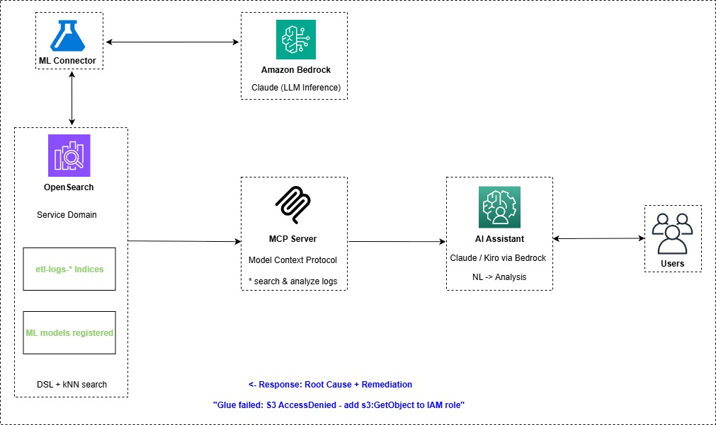
This solution uses CloudWatch real-time streaming to centralize the logs in Amazon OpenSearch Service. With an OpenSearch MCP server running on Amazon Bedrock AgentCore, engineers can identify issues and receive recommendations through the ETL analysis agent.

Architecture diagram showing ETL logs streaming through CloudWatch into Amazon OpenSearch Service, queried by an MCP server on Amazon Bedrock AgentCore

Figure 1: Solution architecture that streams ETL logs into Amazon OpenSearch Service and queries them through an MCP server on Amazon Bedrock AgentCore

Prerequisites

Before deploying this solution, make sure you have the following in place:

AWS account and AWS Region

An active AWS account with access to the US East (N. Virginia) us-east-1 Region. CloudFormation stacks must be deployed in us-east-1.

IAM permissions

An AWS Identity and Access Management (IAM) user or role with permissions to create and manage the following AWS resources:

  • Amazon OpenSearch Service (domain creation, fine-grained access control).
  • Amazon MWAA (environment creation, DAG execution).
  • Amazon MWAA Serverless (workflow creation and execution, a versioned S3 bucket for the workflow definition, and a workflow execution role that requires iam:PassRole).
  • AWS Glue (job creation and execution).
  • Amazon EC2 (instance launch, security groups).
  • Amazon Simple Storage Service (Amazon S3) (bucket creation, object management).
  • AWS Lambda (function creation and execution).
  • Amazon CloudWatch Logs (log group creation, subscription filters).
  • Amazon SageMaker AI (notebook instance creation).
  • Amazon Bedrock (model access, and the AgentCore runtime, a capability of Amazon Bedrock AgentCore).
  • Amazon Cognito (user pool creation).
  • Amazon Elastic Container Registry (Amazon ECR) (repository creation).
  • AWS CodeBuild (project creation).
  • AWS CloudFormation (stack creation with IAM resources).
  • AWS Secrets Manager (secret creation).
  • IAM (role and policy creation).

Amazon Bedrock model access

Enable access to the Anthropic Claude Sonnet model in the Amazon Bedrock console. Navigate to Model access in the Amazon Bedrock console and request access if it isn’t already enabled.

CloudFormation templates

Download the three CloudFormation template files (opensearch_cfn.yaml, etl.yaml, and agentcore-mcp-server.yaml) from the provided GitHub repository before beginning deployment.

Networking

The ETL stack creates a new virtual private cloud (VPC) (CIDR 10.192.0.0/16 by default). Check that this CIDR range doesn’t conflict with existing VPCs in your account if you plan to set up VPC peering or connectivity.

Architecture

The architecture uses Amazon MWAA (provisioned and serverless) as the orchestration layer. As a managed Apache Airflow service, Amazon MWAA lets teams author complex, dependency-aware pipelines as code and schedule, retry, and monitor them without provisioning or operating any Airflow infrastructure. An Airflow DAG defines the pipeline workflow, triggering AWS Glue ETL jobs and Python scripts running on Amazon EC2 instances. Each of these components generates logs that flow into Amazon CloudWatch Logs: Amazon MWAA through its native integration, AWS Glue through its default log group configuration, and Amazon EC2 through the CloudWatch agent.

CloudWatch subscription filters provide the bridge between log storage and analysis. When configured, these filters immediately start streaming real-time log data from selected log groups to Amazon OpenSearch Service. This approach means that data doesn’t need to be copied or duplicated. The subscription filter creates a real-time streaming pipeline that indexes logs as they arrive.

Within OpenSearch, the ML Connector framework integrates with Amazon Bedrock to provide large language model (LLM)-based inference over the log indices. The OpenSearch MCP (Model Context Protocol) server then exposes these capabilities to AI assistants, so users can query their pipeline logs using natural language to identify errors, understand failure patterns, and receive contextual remediation suggestions.

Orchestration and log generation

The architecture begins with Amazon MWAA as the orchestration layer. An Airflow DAG defines the pipeline workflow, triggering AWS Glue ETL jobs and Python scripts running on Amazon EC2 instances. Each of these components generates logs that flow into Amazon CloudWatch Logs.

Workflow

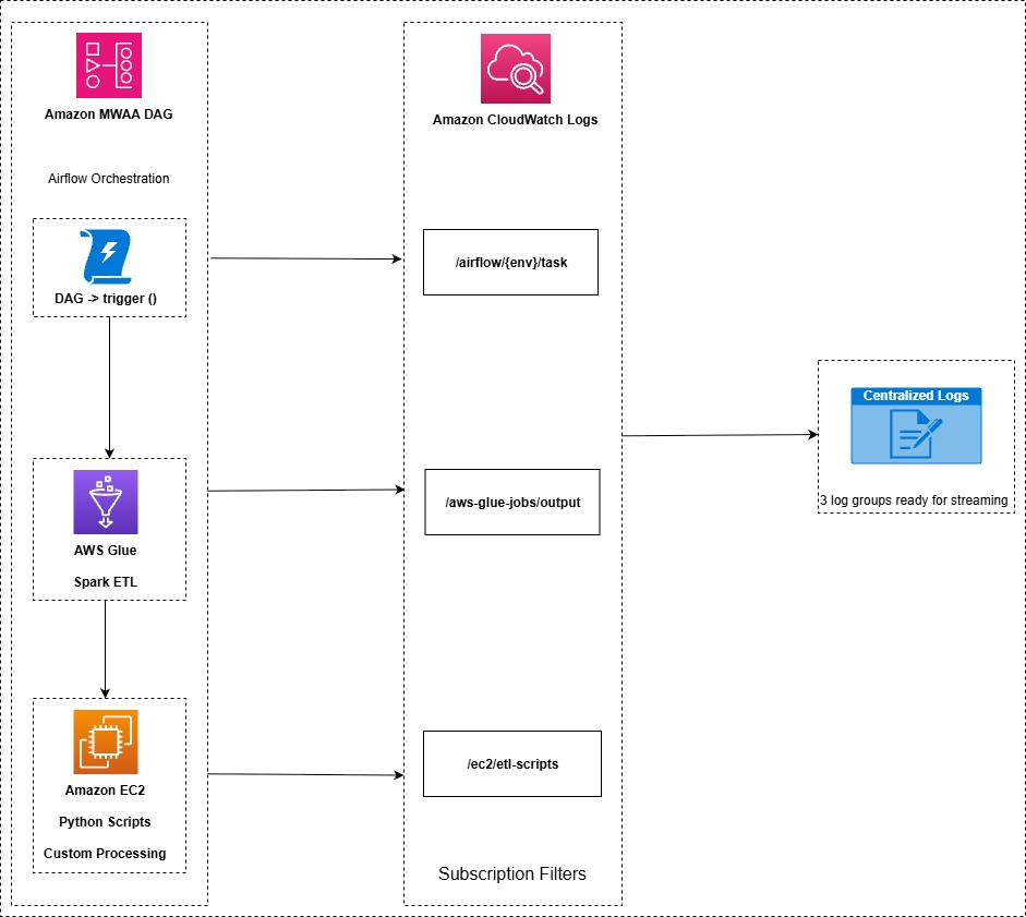
The Amazon MWAA DAG triggers the ETL workflow on a scheduled or event-driven basis. AWS Glue jobs run Spark-based transformations, and logs flow automatically to the /aws-glue/ CloudWatch log group. In parallel, Amazon EC2 Python scripts run custom processing logic and send their logs to CloudWatch. Amazon MWAA task logs automatically land in /airflow/{env}/ log groups. Finally, the CloudWatch unified agent ships logs to the designated log group, where they can be queried through the OpenSearch MCP server.

Log integration methods

Component Integration Log group
Amazon MWAA Native integration /airflow/{env}/task
AWS Glue Default log configuration /aws-glue/jobs/output
Amazon EC2 scripts CloudWatch unified agent /ec2/etl-scripts
Diagram showing Amazon MWAA, AWS Glue, and Amazon EC2 components sending logs to separate Amazon CloudWatch log groups

Figure 2: Log generation and integration across Amazon MWAA, AWS Glue, and Amazon EC2 components

Real-time log streaming

CloudWatch subscription filters provide the bridge between log storage and analysis. When configured, these filters immediately start streaming real-time log data from selected log groups to Amazon OpenSearch Service. This approach means that data doesn’t need to be copied or duplicated. The subscription filter creates a real-time streaming pipeline that indexes logs as they arrive.

Process

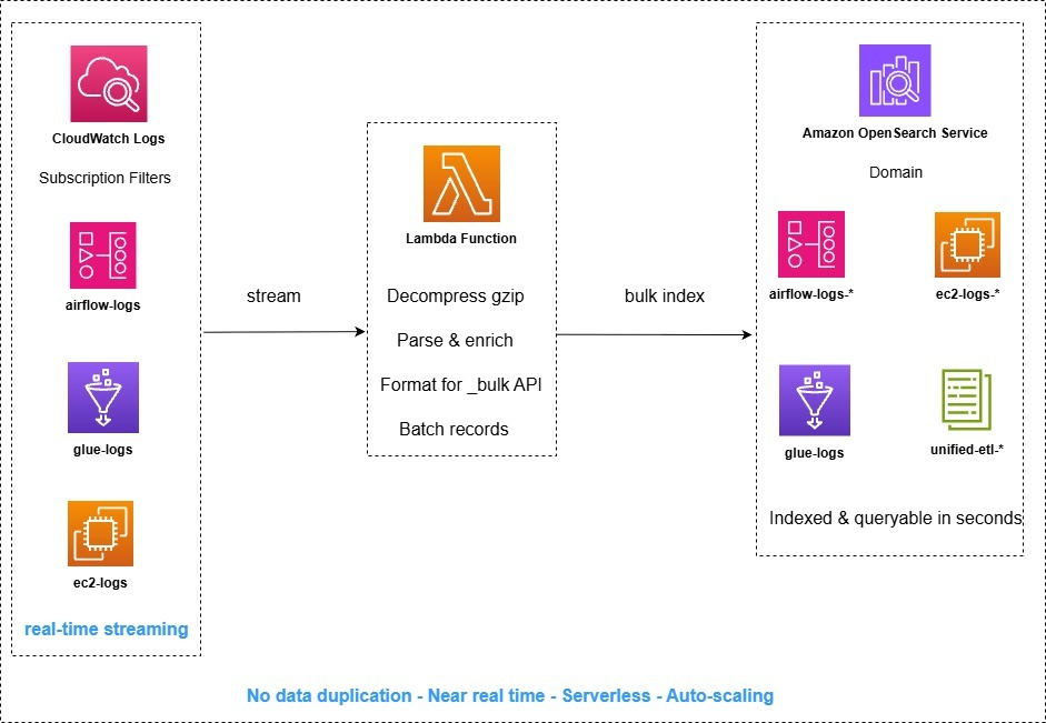
  1. Subscription filters are configured on each CloudWatch log group to match incoming log events.
  2. An AWS Lambda function decompresses gzip-encoded log data, parses and enriches records, and formats them for the OpenSearch Bulk API.
  3. Transformed data is bulk-indexed into Amazon OpenSearch Service domain indices (airflow-logs-*, glue-logs-*, ec2-logs-*, unified-etl-*).
Diagram showing CloudWatch subscription filters streaming log data through an AWS Lambda function into Amazon OpenSearch Service indices

Figure 3: Real-time log streaming from CloudWatch through AWS Lambda into Amazon OpenSearch Service indices

AI-powered analysis and MCP interface

Within OpenSearch, the ML Connector framework integrates with Amazon Bedrock to provide LLM-based inference over the log indices. The OpenSearch MCP (Model Context Protocol) server then exposes these capabilities to AI assistants, so users can query their pipeline logs using natural language to identify errors, understand failure patterns, and receive contextual remediation suggestions.

Process

  1. A user submits a natural language query through the AI assistant (for example, “Why did the Glue job fail at 3 AM?”).
  2. The MCP server translates the query into OpenSearch DSL with ML-enhanced ranking and semantic search.
  3. The ML Connector invokes Amazon Bedrock (Claude) for semantic understanding, log summarization, and pattern detection.
  4. The AI assistant returns root cause analysis with specific remediation steps to the user.
Diagram showing a natural language query flowing through the MCP server and ML Connector to Amazon Bedrock and returning analysis

Figure 4: AI-powered log analysis flow from a natural language query to root cause and remediation guidance

Key architectural benefits

  • Zero data duplication: Subscription filters stream data directly without batch exports, S3 staging, or data copying.
  • Near real-time: Logs are indexed in OpenSearch shortly after generation in source systems.
  • Natural language: Users query logs conversationally through MCP, with no need to write OpenSearch DSL manually.
  • Reduced mean time to resolution: Root cause and remediation recommendations are delivered in a single query, reducing mean time to resolution.
  • Unified view: ETL components are observable through a single search interface.
  • Managed services: There’s no infrastructure to provision, patch, or maintain.

CloudFormation stacks

The solution is split into three CloudFormation stacks. Each template provides a distinct layer of the pipeline.

Stack Template file Deploy time Purpose
opensearch-cfn opensearch_cfn.yaml ~15–20 min OpenSearch domain, SageMaker AI notebook, IAM roles
etl etl.yaml ~25–30 min VPC, Amazon MWAA, AWS Glue, Amazon EC2, log streaming pipeline
agentcore-mcp-server agentcore-mcp-server.yaml ~8–12 min Amazon Bedrock AgentCore MCP Server with Amazon Cognito authentication

Stack 1: opensearch-cfn (opensearch_cfn.yaml)

This stack provisions the foundational OpenSearch domain along with a classic SageMaker AI notebook instance for interactive exploration. This stack creates:

  • An Amazon OpenSearch Service domain (OpenSearch 3.5) with fine-grained access control.
  • A SageMaker AI notebook instance preloaded with workshop lab notebooks.
  • S3 buckets for ETL data, DAGs, and more.
  • IAM roles for notebook and Amazon Bedrock access.
  • A Secrets Manager secret for OpenSearch credentials.
Parameter Default Description
OpenSearchUsername admin Admin username for the OpenSearch cluster
OpenSearchPassword (secure) Admin password (8–32 chars, letters + numbers + symbols)

Stack 2: etl (etl.yaml)

This stack provisions the ETL resources: the networking, orchestration, compute, and log streaming pipeline that feeds OpenSearch. This stack creates:

  • A VPC with private subnets and a NAT gateway for Amazon MWAA networking.
  • An Amazon MWAA environment running an Airflow DAG.
  • An AWS Glue ETL job (reads XLSX, drops a column, writes JSON).
  • An Amazon EC2 instance running a parallel Python ETL script.
  • An Amazon MWAA Serverless workflow for aggregation.
  • S3 buckets for DAG storage and ETL data.
Parameter Default Description
EC2InstanceType t3.micro EC2 instance type for the ETL script
VpcCIDR 10.192.0.0/16 CIDR block for the Amazon MWAA VPC
OpenSearchStackName opensearch-cfn Name of the OpenSearch stack (for cross-stack imports)

Stack 3: agentcore-mcp-server (agentcore-mcp-server.yaml)

This stack deploys an Amazon Bedrock AgentCore MCP Server that exposes OpenSearch tools (ListIndexTool, IndexMappingTool, SearchIndexTool) for natural language log queries. It includes Amazon Cognito authentication and a containerized MCP server built through CodeBuild. This stack creates:

  • An Amazon Bedrock AgentCore runtime hosting the OpenSearch MCP server.
  • An Amazon Cognito user pool for OAuth authentication.
  • An Amazon ECR repository for the MCP server container.
  • A CodeBuild project to build and deploy the container.
Parameter Default Description
MultimodalStackName opensearch-cfn OpenSearch stack name (for importing domain endpoint)
AgentCoreMCPServerName opensearch_mcp_server MCP server name (max 35 chars, appended with unique ID)
AmazonOpenSearchEndpoint (auto-import) Leave blank to auto-import from opensearch-cfn stack
ExecutionRole (auto-create) Leave blank to create a new role
ECRRepository (auto-create) Leave blank to create a new ECR repo
OAuthDiscoveryURL (auto-create Cognito) Leave blank to create a new Amazon Cognito user pool

Deployment order: opensearch-cfn, followed by etl and agentcore-mcp-server. The etl and agentcore-mcp-server CloudFormation templates use outputs from opensearch-cfn.

Implementation

Deploy each CloudFormation stack in sequence

  1. Deploy the OpenSearch infrastructure for opensearch-cfn.
  2. Go to the AWS CloudFormation console, confirm you are in us-east-1, and confirm that Amazon Bedrock is available.

    AWS CloudFormation console with the Region set to US East (N. Virginia)

    Figure 5: Confirming the us-east-1 Region in the AWS CloudFormation console

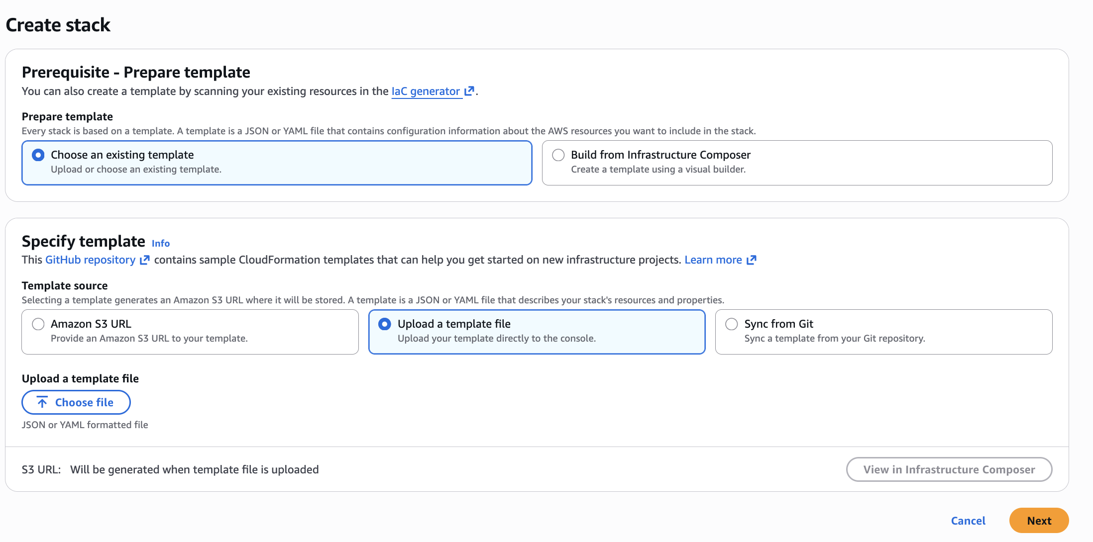
  3. Create the stack. Choose Create stack (with new resources), and then choose an existing template. Select Upload a template file, choose the opensearch-cfn YAML file, and choose Next.

    Create stack page in AWS CloudFormation with Upload a template file selected

    Figure 6: Uploading the opensearch-cfn template on the Create stack page

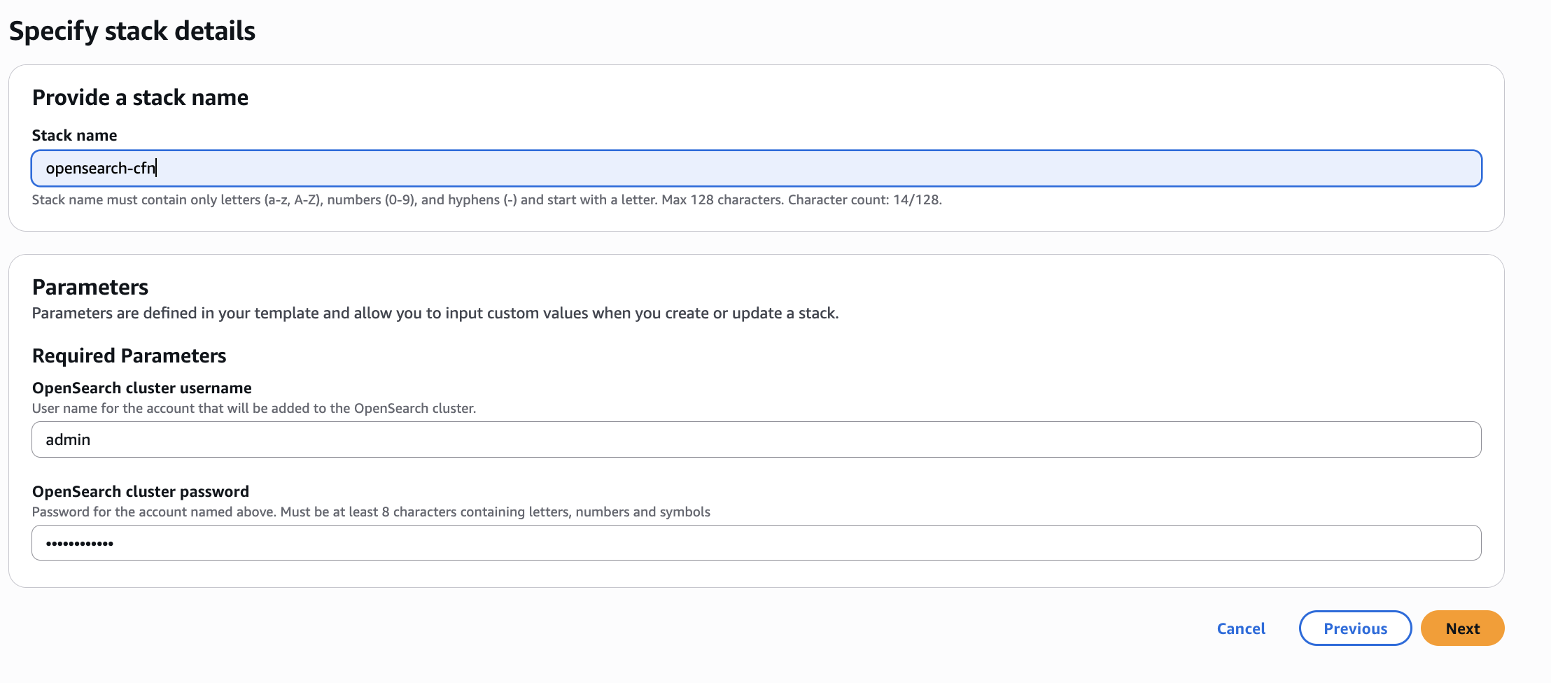
  4. Configure stack options. For stack name, enter opensearch-cfn, leave the parameters as their defaults, and choose Next.

    Configure stack options page showing the stack name opensearch-cfn

    Figure 7: Entering the stack name on the Configure stack options page

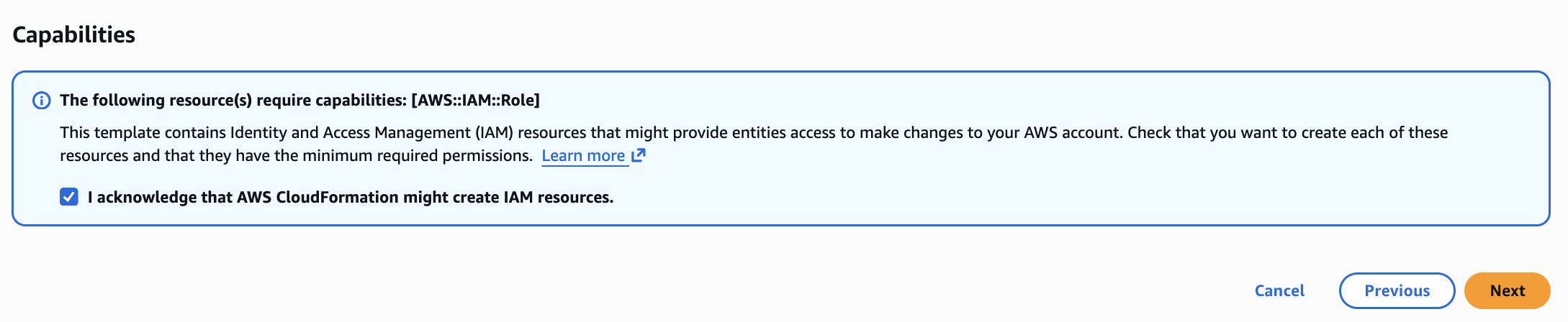
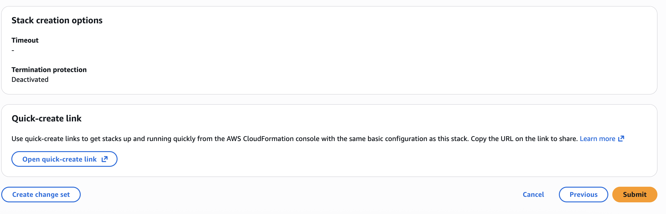
  5. Review and deploy. Review the parameter summary, then scroll to the bottom and select I acknowledge that AWS CloudFormation might create IAM resources with custom names. Choose Next, and then choose Submit.
    CloudFormation review page with the IAM capabilities acknowledgment checkbox selected

    Figure 8: Acknowledging IAM resource creation on the review page

    CloudFormation review page ready to submit the stack

    Figure 9: Reviewing and submitting the stack

    Wait for the stack to complete until its status changes to CREATE_COMPLETE.

  6. Deploy the ETL stack the same way. Set the stack name to etl, leave the parameters as their defaults, and wait for the status to change to CREATE_COMPLETE.
  7. Deploy the agentcore-mcp-server stack the same way. Set the stack name to agentcore-mcp-server, leave the parameters as their defaults, and wait for the status to change to CREATE_COMPLETE.

Work with the SageMaker AI notebook

  1. Open the SageMaker AI notebook. Go to AWS CloudFormation on the AWS Management Console and select the opensearch-cfn stack.
  2. Select the Outputs tab, scroll down, and open the URL for the SageMaker AI notebook.
  3. After SageMaker AI has loaded, select Lab-OpenSearch-Observability.ipnyb from the left side menu to open the notebook.
  4. Run each cell in order. To do this, select the cell and then choose the play button (the right-facing triangle).
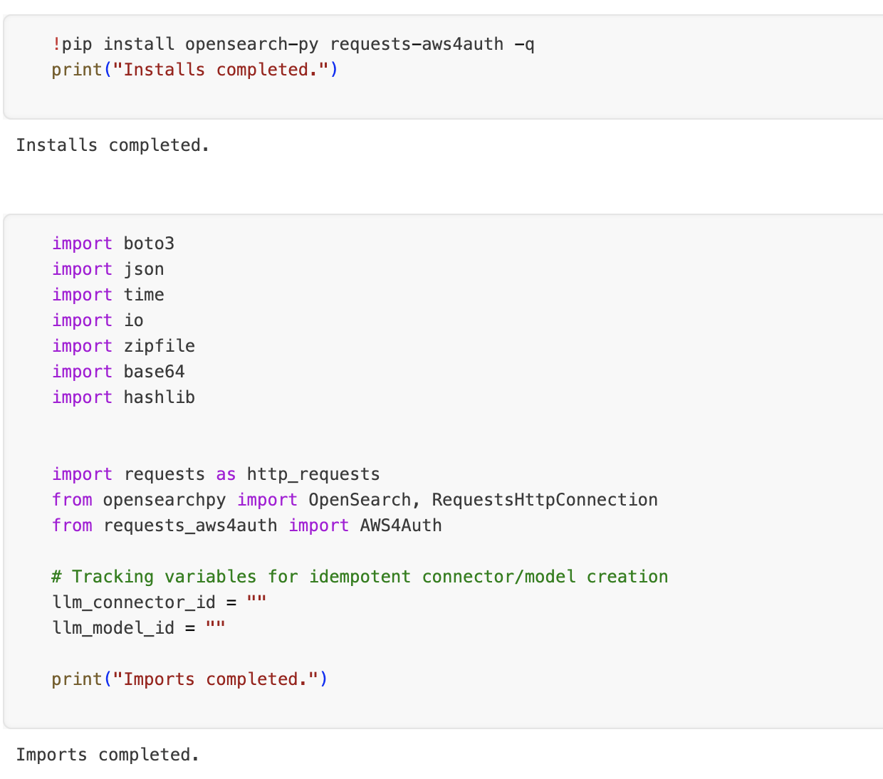
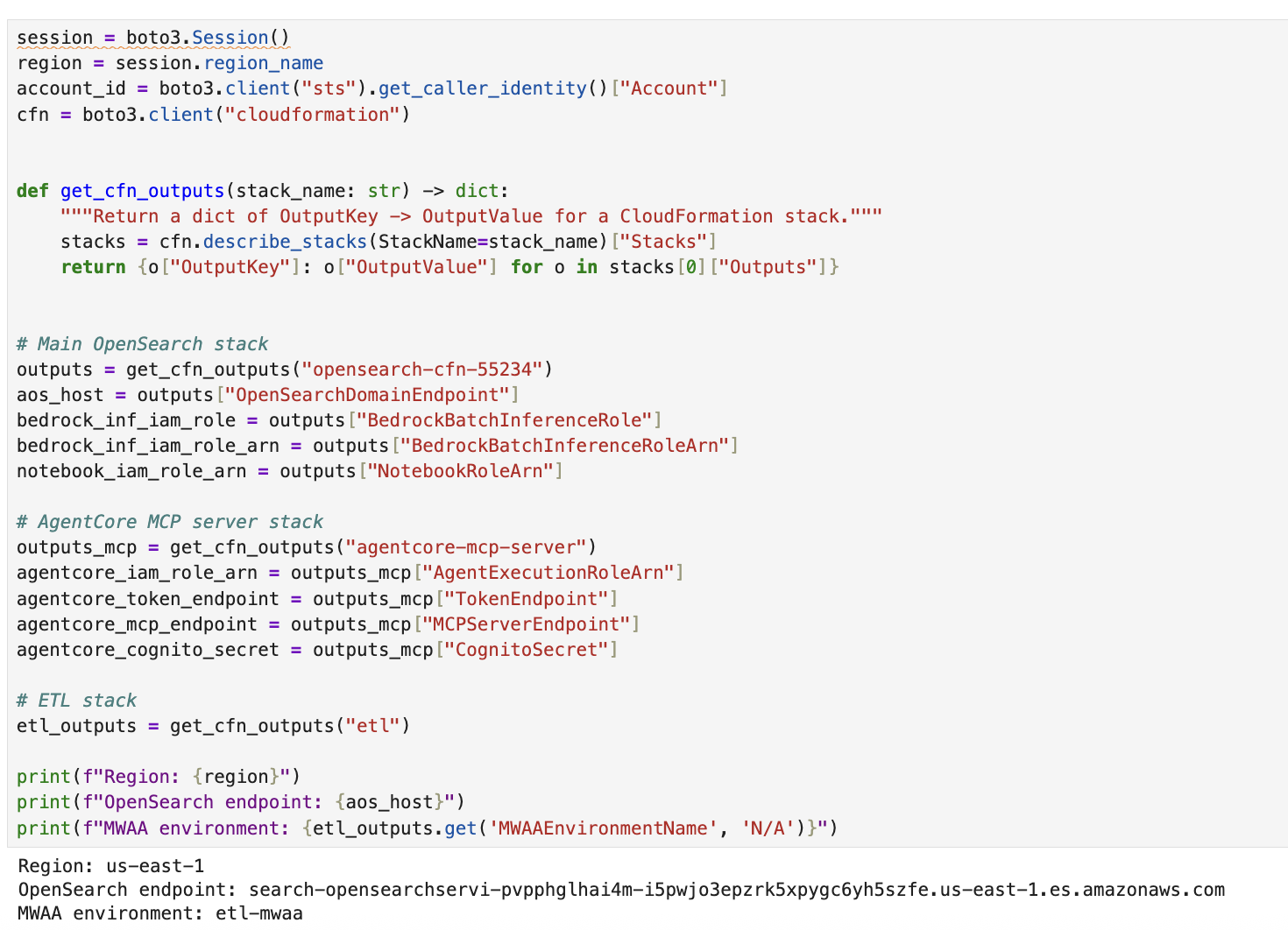
  5. Complete the prerequisites. Section 1 of the notebook loads the required Python modules to run the code in this notebook. It also retrieves resource metadata for the resources created by the CloudFormation stacks. These cells need to run before you move to section 2.
    Notebook cell that loads the required libraries and imports the Python modules

    Figure 10: Load the required libraries and import the Python modules

    Notebook cell that loads the CloudFormation stack outputs

    Figure 11: Load the CloudFormation stack outputs

  6. Section 2: Connect to OpenSearch.
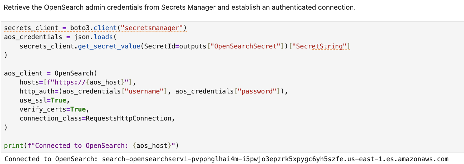
    Notebook cell that retrieves the OpenSearch admin credentials from Secrets Manager

    Figure 12: Authenticate by retrieving the OpenSearch admin credentials from Secrets Manager

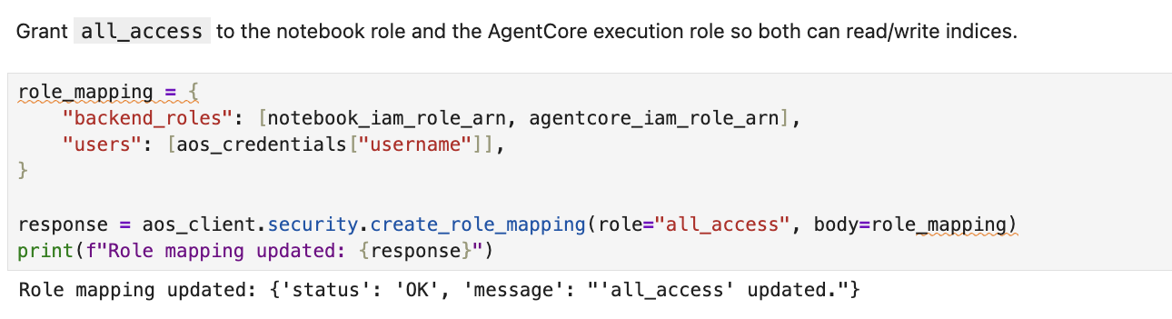
    Notebook cell that grants OpenSearch access to the notebook role and the AgentCore execution role

    Figure 13: Grant access to the notebook role and the AgentCore execution role

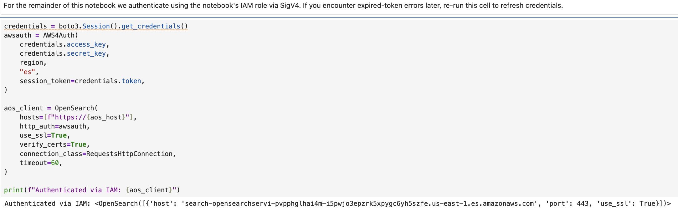
    Notebook cell that switches OpenSearch to IAM-based authentication

    Figure 14: Switch to IAM-based authentication

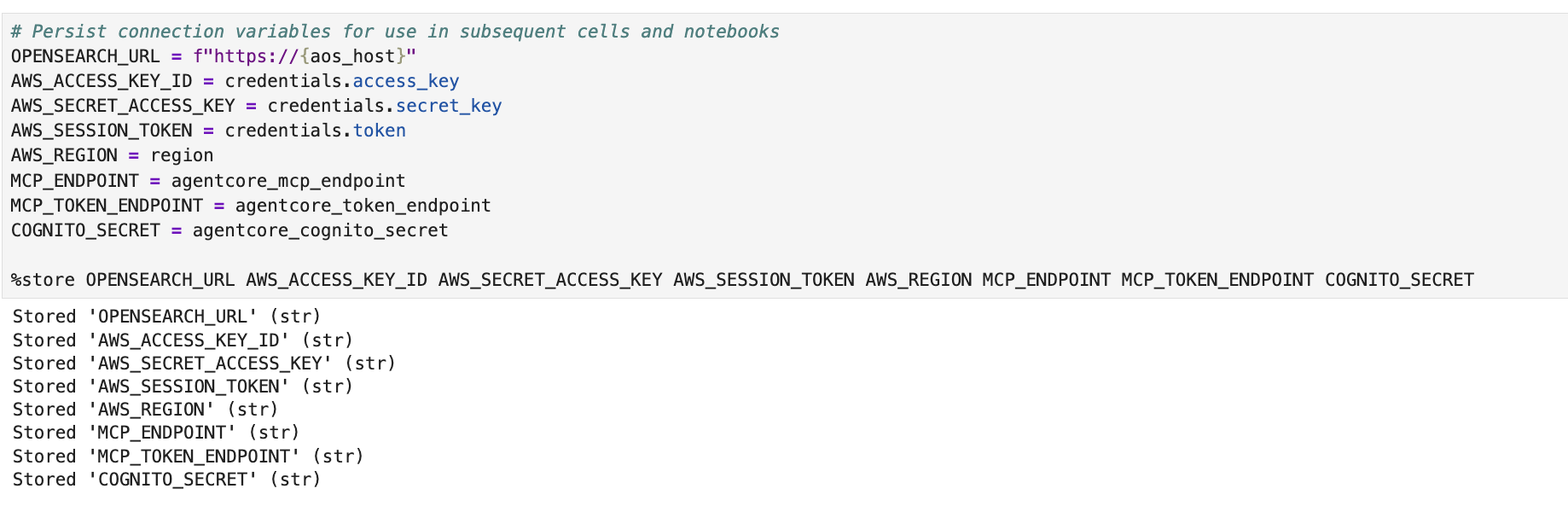
    Notebook cell that persists the OpenSearch connection variables

    Figure 15: Persist connection variables for use in subsequent cells and notebooks

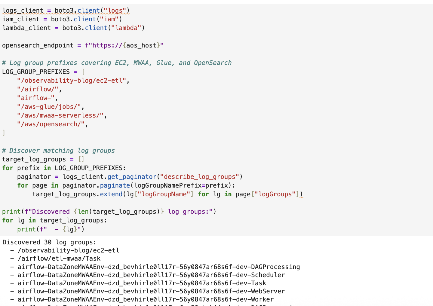
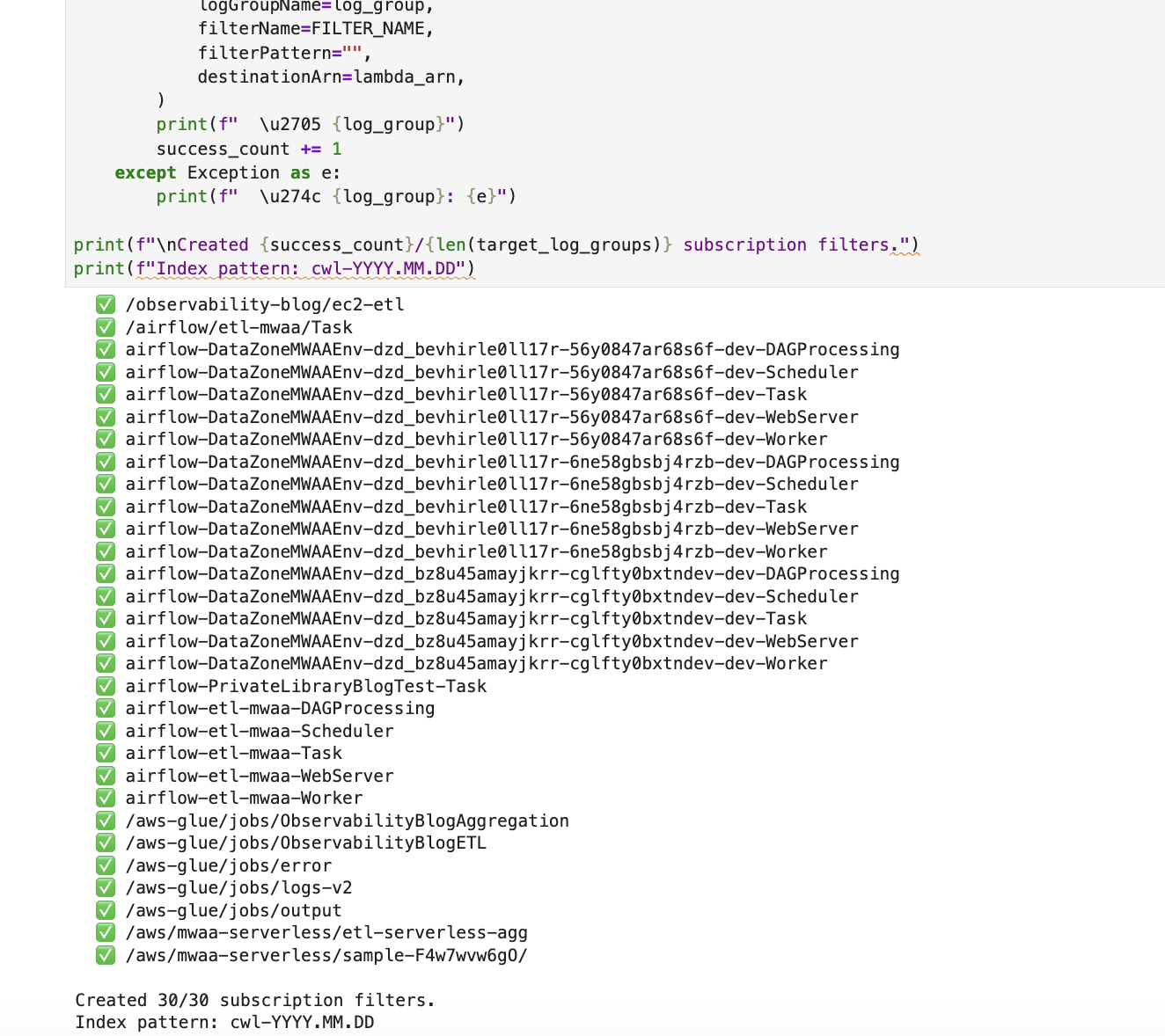
  7. Section 3: Stream CloudWatch Logs into OpenSearch.
    Notebook cell that creates a Lambda function and CloudWatch subscription filters

    Figure 16: Create the Lambda function and CloudWatch subscription filters that stream ETL-related log groups into OpenSearch indices

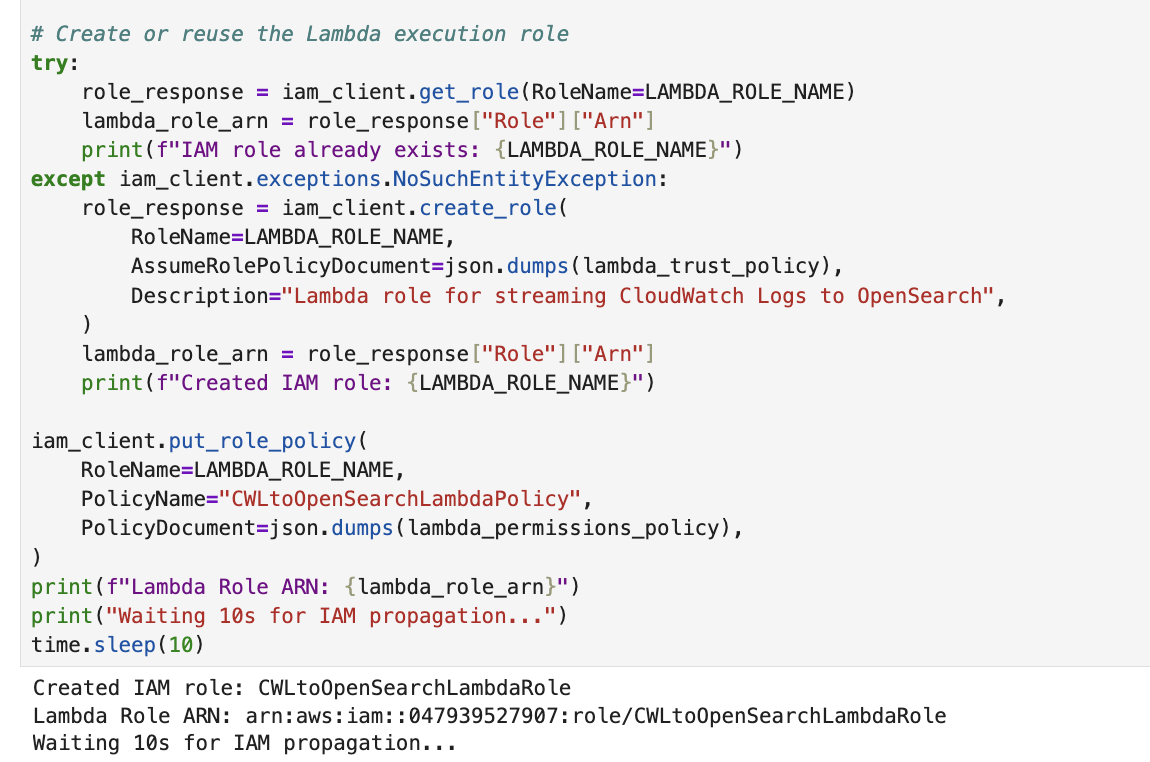
    Notebook cell that creates an IAM role for the Lambda function

    Figure 17: Create the IAM role for the Lambda function

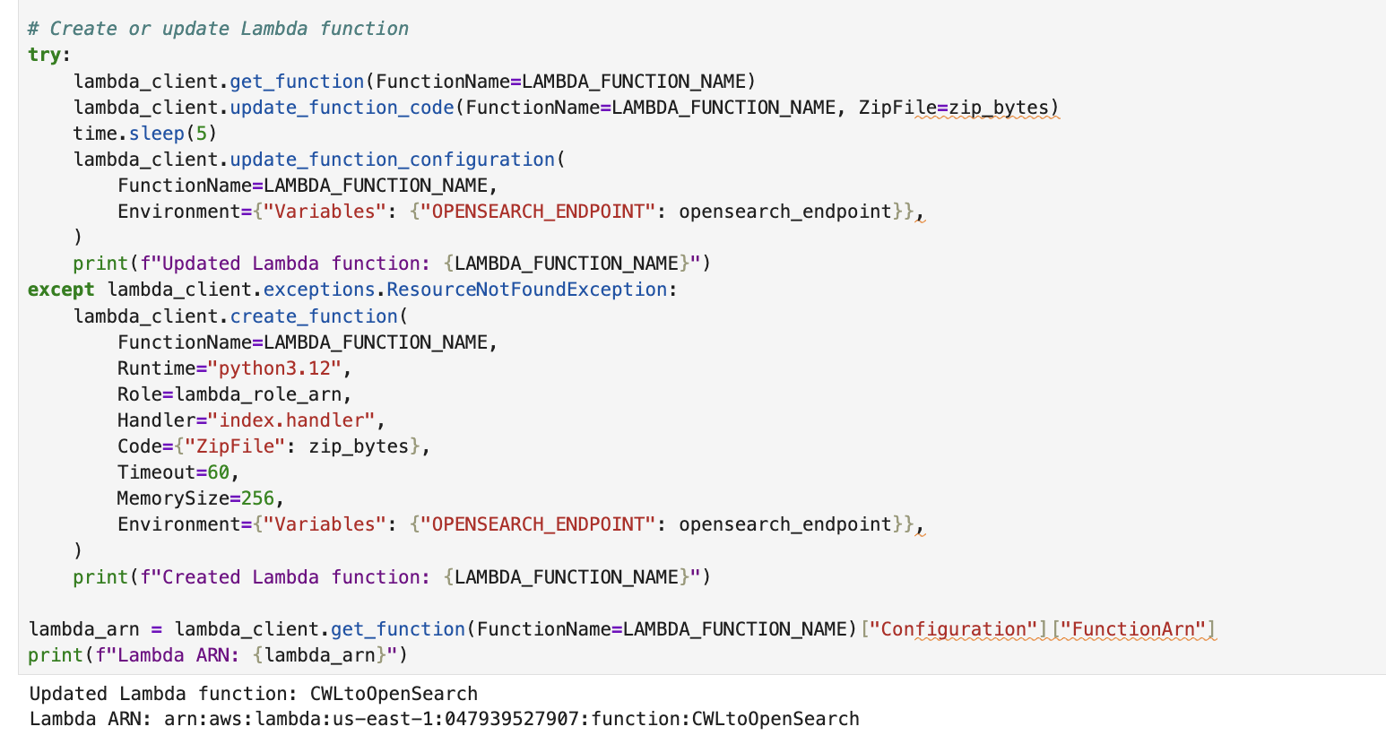
    Notebook cell that creates the Lambda function

    Figure 18: Create the Lambda function

    Notebook cell that grants CloudWatch Logs permission to invoke the Lambda function

    Figure 19: Grant CloudWatch Logs permission to invoke the Lambda function

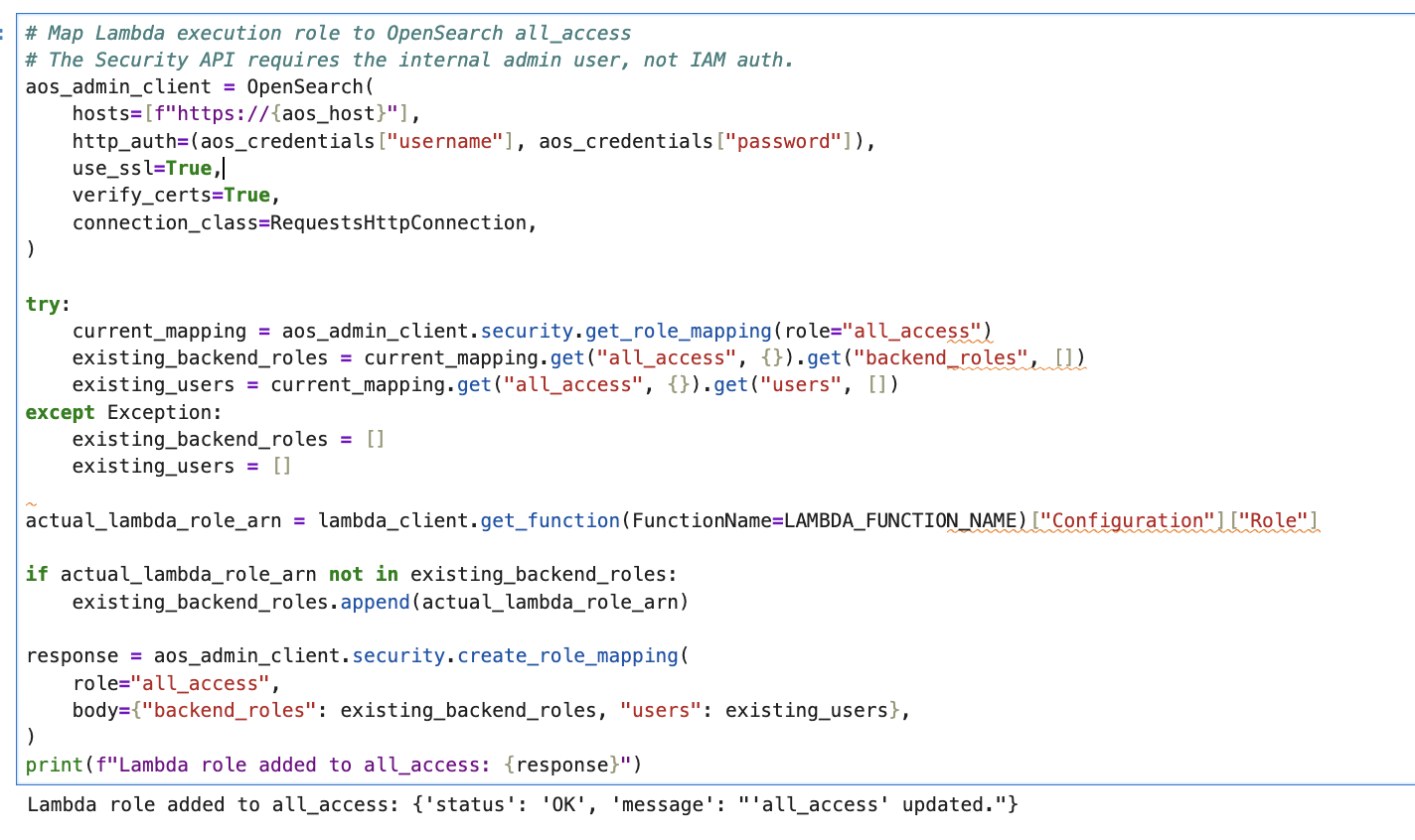
    Notebook cell that maps the Lambda execution role to the OpenSearch all_access role

    Figure 20: Map the Lambda execution role to the OpenSearch all_access role

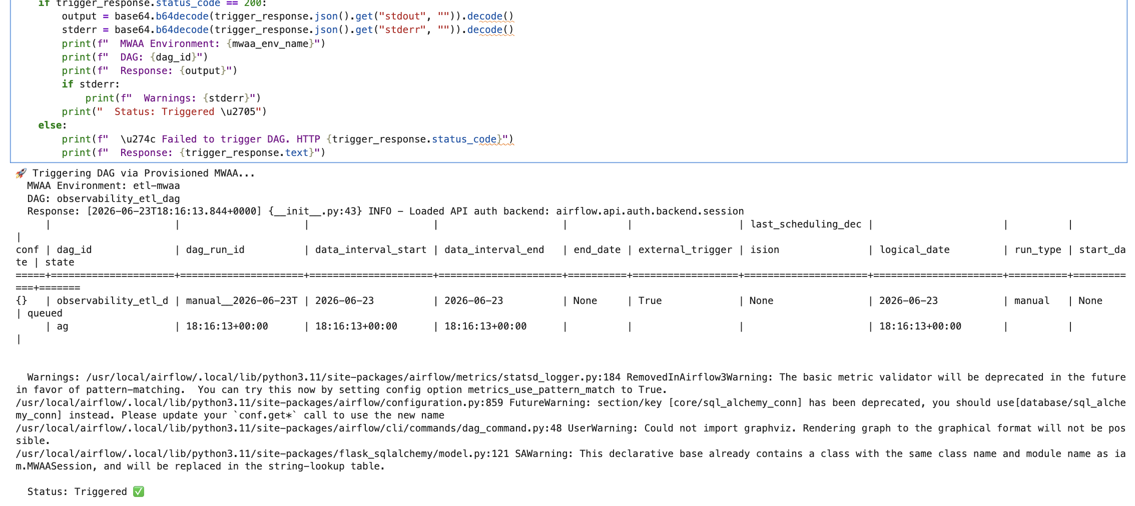
  8. Section 4: Trigger the ETL DAG.

    Trigger the ETL DAG and generate logs through the USE_SERVERLESS flag to select your preferred runtime environment.

    When set to False (the default), the observability_etl_dag DAG runs on provisioned Amazon MWAA, running AWS Glue and Amazon EC2 tasks in parallel. When set to True, the observability_blog_aggregation DAG runs on Amazon MWAA Serverless, running an AWS Glue aggregation job.

    Notebook cell that triggers the ETL DAG

    Figure 21: Trigger the ETL DAG

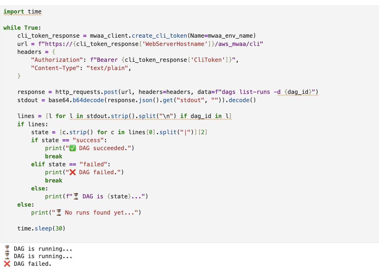
    Notebook output that verifies the DAG has stopped running

    Figure 22: Verify that the DAG has stopped running

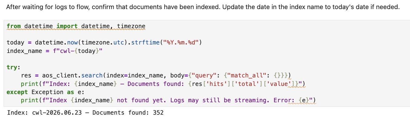
    Notebook output that verifies log ingestion into OpenSearch

    Figure 23: Verify log ingestion

  9. Section 5: Register the Claude LLM connector in OpenSearch.
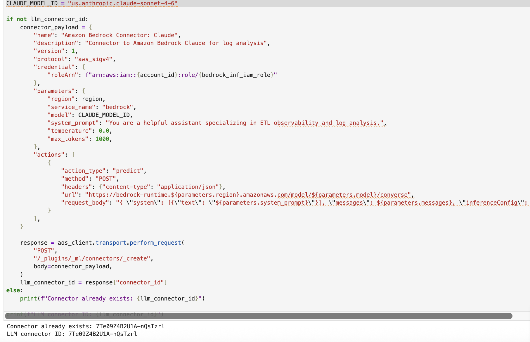
    1. Create an ML connector in OpenSearch that calls the Anthropic Claude model on Amazon Bedrock (us.anthropic.claude-sonnet-4-20250514-v1:0) through the Converse API, using SigV4 authentication and an assumed IAM role.
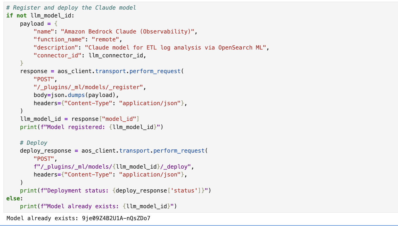
    2. Register and deploy the model so that OpenSearch can use it for ML-powered features such as Retrieval Augmented Generation (RAG) and conversational search.
    Notebook cell that creates the ML connector to the Claude model on Amazon Bedrock

    Figure 24: Create the machine learning connector to the Claude model

    Notebook cell that registers and deploys the model in OpenSearch

    Figure 25: Register and deploy the model in OpenSearch

  10. Section 6: Register the AI agent with the OpenSearch MCP server.
    1. Install the agent libraries (mcp, strands-agents, uv).
    2. Load the Amazon Cognito credentials for authenticating with the AgentCore MCP Server.
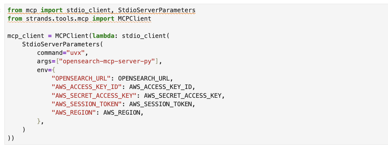
    3. Choose a deployment mode. Option A (local) runs the OpenSearch MCP server as a subprocess through uvx for development.
    Notebook cell that runs the OpenSearch MCP server locally through uvx

    Figure 26: Run the OpenSearch MCP server locally as a subprocess

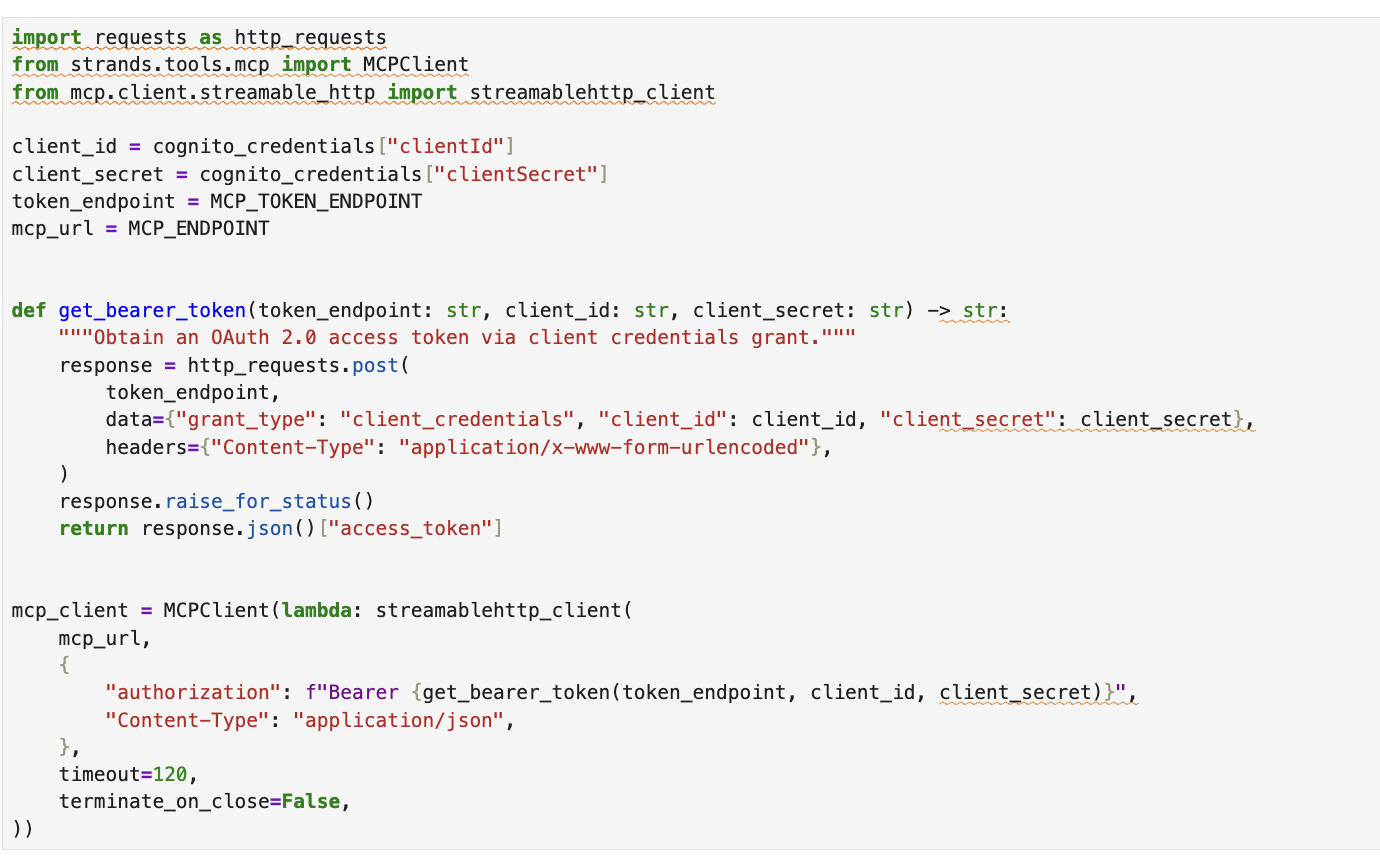
    Option B (AgentCore) connects to a production MCP server on Amazon Bedrock AgentCore using OAuth 2.0 client credentials.

    Notebook cell that connects to the production MCP server on Amazon Bedrock AgentCore

    Figure 27: Connect to the production MCP server on Amazon Bedrock AgentCore

    d. Create the ETL analysis agent.

    Notebook cell that creates the ETL analysis agent

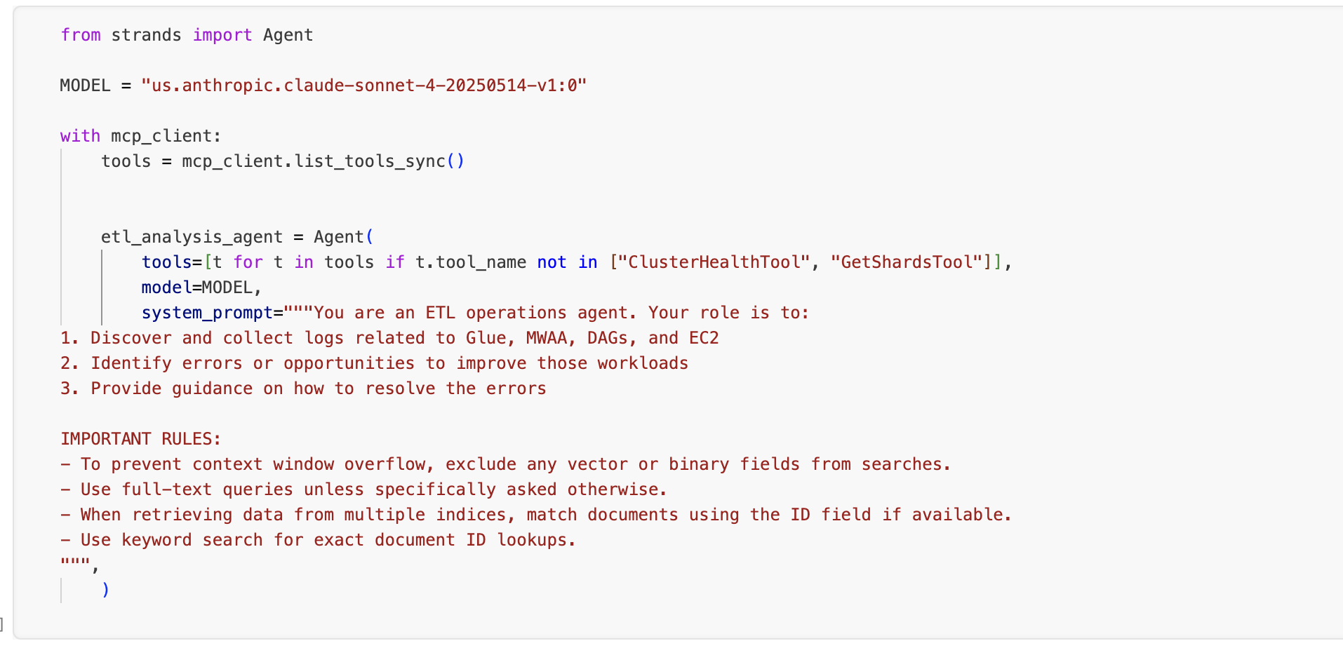
    Figure 28: Create the ETL analysis agent

Results

In section 7 of the notebook, you can ask questions about your ETL pipeline. A sample question is included in the notebook: “What errors do you see in the logs”. Try asking additional questions about the ETL pipeline and related services. The agent autonomously searches indices, correlates events, and returns an analysis of the error with remediation guidance.

Example natural language queries

What you want to find Example prompt
Errors across the sources Show me the ERROR level logs
AWS Glue job success logs Find successful AWS Glue ETL job completions
Amazon EC2 script failures Show me Amazon EC2 ETL script errors with stack traces
Amazon MWAA task failures Find failed Amazon MWAA DAG tasks
Amazon MWAA Serverless workflow logs Show me logs from the Amazon MWAA Serverless aggregation workflow
Recent activity Show me the last 20 log entries from any source
Specific time range Show me logs from the last 30 minutes

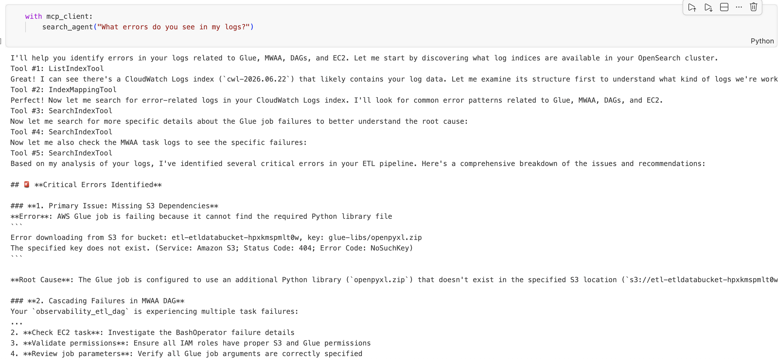
The following screenshot shows a natural language query being sent to the search_agent through the MCP client, with the agent using multiple tools (ListIndexTool, IndexMappingTool, SearchIndexTool) to discover indices, understand intent, and return structured findings from the pipeline-logs index.

MCP client showing a natural language query and the ETL analysis agent’s structured findings from the pipeline-logs index

Figure 29: Example natural language query and the agent’s structured findings

Outcome

After a single CloudFormation deployment and five steps, you have a pipeline that processes tabular data through parallel ETL paths, aggregates the results, and consolidates operational logs into one searchable index. When something breaks, you open one dashboard, type what you are looking for, and get your answer. There is no tab-hopping, no timestamp-matching, and no guessing which service threw the error.

The combination of Amazon MWAA for orchestration, OpenSearch for log aggregation, and Amazon Bedrock for natural language access gives you an observability layer that your team actually uses, because it is faster than the alternative.

Clean up

To remove the services used in this solution, delete the three stacks using the AWS CloudFormation console, or run the following command in the AWS CLI:

aws cloudformation delete-stack --stack-name <stack name>

This removes the provisioned resources, including the OpenSearch domain, Amazon MWAA environment, AWS Glue jobs, Amazon EC2 instance, and associated IAM roles.

Conclusion

Observability for a multi-service ETL pipeline doesn’t need to mean stitching together multiple CloudWatch log groups by hand. By streaming every component’s logs into a single OpenSearch index and putting an Amazon Bedrock model in front of it, you turn “I need to find the right log group and write a filter expression” into “show me errors from AWS Glue in the last hour”.

Where to go from here:

  • Add alerting: configure OpenSearch alerting rules to notify your team through Amazon Simple Notification Service (Amazon SNS) when ERROR-level logs exceed a threshold.
  • Expand the index: add logs from other components (AWS Step Functions, AWS Lambda, and additional AWS Glue jobs) by creating new CloudWatch subscription filters.
  • Build dashboards: use the OpenSearch UI for visualizations, such as error rate over time, log volume by source, and latency between DAG trigger and job completion.
  • Fine-tune the Amazon Bedrock model: adjust the prompt template in the ML connector to include your index mapping, which improves query accuracy for domain-specific questions.
  • Use OpenSearch Ask AI directly from the OpenSearch UI.

The goal is straightforward: when your pipeline fails, you should spend your time fixing the problem, not finding it. Try the solution in your own environment and tell us what you think in the comments.


About the authors

Anupa Bhattacharyya

Anupa Bhattacharyya

Anupa is an Enterprise Support Lead in CIENG at Amazon Web Services, where she guides Enterprise customers through their cloud journey. With over 15 years of experience in data and analytics, she excels in defining strategic initiatives for enterprise customers. Outside of work, she enjoys painting, traveling, family time, and savoring new cuisines.

Sean Bjurstrom

Sean Bjurstrom

Sean is a Technical Account Manager in ISV accounts at Amazon Web Services, where he specializes in analytics technologies and draws on his background in consulting to support customers on their analytics and cloud journeys. Sean is passionate about helping businesses harness the power of data to drive innovation and growth. Outside of work, he enjoys running and has participated in several marathons.

Manikandan Mylsamy

Manikandan Mylsamy

Manikandan is a Technical Account Manager, EC2 SME specializing in Microsoft technologies at AWS ISV accounts. He helps enterprises accelerate cloud adoption and optimize infrastructure for operational excellence. Outside work, he enjoys cricket, swimming, and long drives.

Karthik Seshadri

Karthik Seshadri

Karthik is a Sr. Software Development Engineer in AWS, where he specializes in orchestration of big data technologies. He is enthusiastic about serverless technologies, data engineering and building great services. Outside of work, he enjoys traveling and playing various sports.

Cost-effective ETL with DuckDB and Amazon S3 Tables on AWS Glue

Post Syndicated from Bezuayehu Wate original https://aws.amazon.com/blogs/big-data/cost-effective-etl-with-duckdb-and-amazon-s3-tables-on-aws-glue/

Many data integration jobs are SQL-centric: they filter, join, and aggregate data on a schedule, and they run frequently enough that fast startup matters. For this shape of work, teams want to match the engine to the job and run it quickly and cost-effectively, without standing up and tuning separate infrastructure.

AWS Glue is the serverless data integration service that customers use to run extract, transform, and load (ETL) jobs at any scale, without managing infrastructure. With AWS Glue, you can run DuckDB, an embedded, in-process, vectorized SQL engine, inside a standard AWS Glue job. DuckDB reads Parquet files from Amazon Simple Storage Service (Amazon S3) and writes Apache Iceberg tables directly to Amazon S3 Tables, a capability of Amazon S3. DuckDB is an open source, in-process, vectorized analytical SQL engine that runs embedded in your application, with no separate server or cluster to manage. It reads and writes cloud data formats such as Parquet and Apache Iceberg natively. AWS Glue 6.0 is the latest version, running on a modernized runtime with a 30 percent price reduction over previous versions. DuckDB reads Amazon S3 Parquet through its httpfs extension and commits Iceberg snapshots to Amazon S3 Tables through the Iceberg REST endpoint, so no separate catalog synchronization is required. Running DuckDB in AWS Glue is well suited to SQL-centric transformations such as filters, joins, and aggregations. It also fits frequent, scheduled jobs such as hourly or daily aggregations, incremental loads, and rollups that benefit from fast startup. This pattern complements Apache Spark on AWS Glue rather than replacing it: when a workload needs distributed processing, the same job type runs PySpark with no change to your infrastructure, IAM, or triggers.

This post walks through the pattern with a concrete ETL use case and provides complete, runnable code. It also compares measured cost and runtime against a Spark job performing the same work on the same AWS Glue 6.0 runtime.

When to use this pattern

This pattern is a complement to Spark on AWS Glue, not a replacement. The following table summarizes when each approach yields the best results.

Signal

DuckDB on AWS Glue 6.0

Apache Spark on AWS Glue 6.0

Dataset size per run Scales with worker size Scales horizontally across multiple nodes for datasets of any size
Parallelism requirement Single-node, in-process execution Distributed processing across a managed cluster
SQL complexity Aggregations, joins, window functions Complex graph operations, custom UDFs, ML pipelines
Cost priority Minimize per-run cost and duration Maximize throughput at scale
Iceberg writes DuckDB iceberg extension to S3 Tables Native Spark Iceberg integration

For workloads that need distributed processing, the same glueetl job type runs PySpark with no change to your infrastructure, AWS Identity and Access Management (IAM) configuration, or triggers. You choose the engine that fits each workload.

How DuckDB runs on AWS Glue 6.0

Running DuckDB in an AWS Glue job comes down to two things working together: a runtime modern enough to load DuckDB and its native extensions, and the capabilities DuckDB brings to ETL once it does.

What the AWS Glue 6.0 runtime provides

Modern runtime compatibility. AWS Glue 6.0 runs on Amazon Linux 2023 with glibc 2.34 and Python 3.13. DuckDB 1.5.x and its native C++ extension binaries (httpfs, aws, iceberg) install through pip and load without workarounds. The DuckDB extension binaries require a modern glibc (2.28 or later), which the AWS Glue 6.0 runtime provides.

AWS Glue 6.0 resolves this compatibility requirement. You can add DuckDB 1.5.x to an AWS Glue 6.0 job in two ways. The first is the --additional-python-modules job parameter (duckdb==1.5.1), which pip-installs the package at job startup and loads all extensions without additional steps. Alternatively, you can package the dependencies as a Python virtual environment, upload it to Amazon S3, and reference it using the --python-virtual-env parameter. On AWS Glue 6.0, you can also add --python-virtual-env-storage-prefix to have AWS Glue build and cache the virtual environment automatically. For more information, see Using Python virtual environments with AWS Glue.

What DuckDB provides

DuckDB is an open source, in-process analytical SQL engine. It runs inside an AWS Glue job as a single process, with no separate cluster or coordinator. The following capabilities make it a practical fit for ETL on the AWS Glue 6.0 runtime.

  • Single-node vectorized execution. DuckDB runs inside a single AWS Glue job. For a couple of gigabytes, there is no shuffle, no executor scheduling, and no inter-node network I/O. The work happens in a single vectorized pass over columnar memory.
  • Native Amazon S3 and Parquet access. The httpfs extension reads and writes Amazon S3 objects directly, using the IAM role of the AWS Glue job automatically through CREDENTIAL_CHAIN.
  • Native Amazon S3 Tables writes. The iceberg extension connects to the Amazon S3 Tables Iceberg REST endpoint (ENDPOINT_TYPE s3_tables) and commits standard Iceberg snapshots. With AWS Glue 6.0, you can use two capabilities that matured independently: Amazon S3 Tables and DuckDB Iceberg writes.
  • Larger-than-memory operators. Sort, join, and aggregate spill to /tmp, so datasets larger than available RAM still process without code changes.

The output is a standard Apache Iceberg table in Amazon S3 Tables. It is queryable by Amazon Athena, Amazon Redshift, and Amazon EMR, and other Iceberg-compatible engines that support the Iceberg REST Catalog API.

Sizing guidance. DuckDB runs within a single AWS Glue worker, so its available memory and disk scale with the worker type. This walkthrough uses the minimum glueetl configuration of 2 workers (2 data processing units, or DPUs) with worker type G.1X: each G.1X worker provides 4 vCPUs and 16 GB of memory. DuckDB runs on the driver and processes data in memory, spilling to local disk when a dataset or intermediate result exceeds available RAM. For larger inputs, choose a bigger worker: G.2X provides 8 vCPUs and 32 GB of memory, and the G.4X and G.8X types scale higher. Size the worker to your input volume and the memory footprint of your aggregations and joins. For current specifications, see AWS Glue worker types.

Architecture

The following image shows the architecture described in this post.

Architecture diagram: raw Parquet files in Amazon S3 flow into an AWS Glue 6.0 job running DuckDB, which writes Apache Iceberg tables to Amazon S3 Tables, with Amazon Athena and Amazon QuickSight querying the output.

Figure 1: Data flows from raw Parquet in Amazon S3 through an AWS Glue 6.0 job running DuckDB, which writes Apache Iceberg tables to Amazon S3 Tables for querying by Amazon Athena and Amazon QuickSight.

The pipeline consists of the following managed components:

Layer

Role

AWS Service

Source Raw Parquet files, partitioned by date Amazon S3
Compute DuckDB SQL engine running on the AWS Glue 6.0 runtime AWS Glue 6.0 (glueetl)
Destination Iceberg analytical tables, queryable by any engine Amazon S3 Tables
Governance Permissions and access control for S3 Tables writes AWS Lake Formation
Query Analytics and business intelligence (BI) on the output tables Amazon Athena, Amazon QuickSight

Raw Parquet files land in Amazon S3 on a schedule. An AWS Glue 6.0 job runs DuckDB. DuckDB reads the files, applies SQL transformations in memory, and writes the aggregated result as an Iceberg table to Amazon S3 Tables through the Iceberg REST catalog. Amazon Athena and Amazon QuickSight can query the output immediately. No separate catalog synchronization is required.
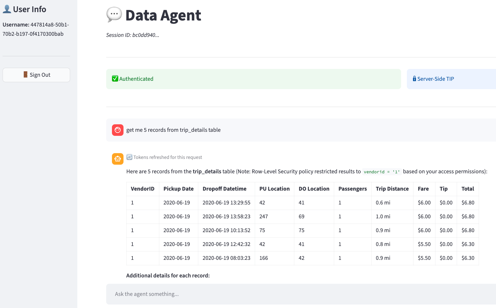
You can trigger the job several ways:

Walkthrough: eCommerce daily order summary

This section walks through a daily ETL pipeline for an eCommerce application. The pipeline reads raw transaction files from Amazon S3, cleanses and aggregates them, and writes a query-ready summary to Amazon S3 Tables.

Step

Operation

Detail

1. Source Read raw Parquet from S3 s3://<amzn-s3-demo-source-bucket>/orders/year=2026/month=08/*.parquet
2. Filter status IN (‘completed’,‘processing’) Drop canceled and test orders
3. Enrich net_revenue, avg_order_value Derived columns via SQL expressions
4. Aggregate GROUP BY order_day, region, category Daily revenue, order count, unique customers
5. Write INSERT into an Amazon S3 Tables Iceberg table Idempotent per-day reload

Prerequisites

  • An AWS account with permissions for AWS Glue, Amazon S3, Amazon S3 Tables, AWS Identity and Access Management (IAM), and AWS Lake Formation.
  • An Amazon S3 bucket containing raw Parquet files (referred to as <amzn-s3-demo-source-bucket> in this post).
  • An Amazon S3 Tables table bucket (referred to as <amzn-s3-demo-table-bucket> in this post). See the Create the S3 Tables table bucket section.
  • An IAM role for the AWS Glue job with:
    • Amazon S3 read access on <amzn-s3-demo-source-bucket>.
    • Amazon S3 Tables read/write access.
    • AWS Glue job execution permissions.
  • AWS Lake Formation grants on the S3 Tables catalog and namespace (required for Iceberg write operations).
  • An AWS Glue 6.0 job (glueetl) with:
    • --additional-python-modules: duckdb==1.5.1.
    • Minimum worker configuration: 2 workers, type G.1X.

Note on DuckDB versions. DuckDB support for writing Apache Iceberg tables through a REST catalog, including Amazon S3 Tables, requires version 1.4.0 or later. This walkthrough uses duckdb==1.5.1. On the AWS Glue 6.0 runtime (Amazon Linux 2023), it installs and all native extensions load without additional configuration.

Create the S3 Tables table bucket

If you don’t already have an Amazon S3 Tables table bucket, create one using the AWS Command Line Interface (AWS CLI):

aws s3tables create-table-bucket \
    --name <amzn-s3-demo-table-bucket> \
    --region <YOUR-REGION>

Note the table bucket Amazon Resource Name (ARN) from the output. It follows the format:

arn:aws:s3tables:<YOUR-REGION>:<YOUR-ACCOUNT-ID>:bucket/<amzn-s3-demo-table-bucket>

Turn on integration with AWS analytics services so the table is discoverable by Amazon Athena, Amazon Redshift, and Amazon EMR. Complete the integration by creating the s3tablescatalog catalog in the AWS Glue Data Catalog using the AWS CLI. For the steps, see Integrating Amazon S3 Tables with AWS analytics services.

After turning on integration, grant the AWS Glue job role Lake Formation permissions on the Amazon S3 Tables catalog and the analytics namespace:

# Allow the job to create the target table on first run (namespace-scoped)
aws lakeformation grant-permissions \
    --principal DataLakePrincipalIdentifier=arn:aws:iam::<YOUR-ACCOUNT-ID>:role/<YOUR-AWS-GLUE-ROLE> \
    --resource '{"Database":{"Name":"analytics","CatalogId":"<YOUR-ACCOUNT-ID>:s3tablescatalog/<amzn-s3-demo-table-bucket>"}}' \
    --permissions '["CREATE_TABLE"]'

# Grant only the operations the job performs on the target table
aws lakeformation grant-permissions \
    --principal DataLakePrincipalIdentifier=arn:aws:iam::<YOUR-ACCOUNT-ID>:role/<YOUR-AWS-GLUE-ROLE> \
    --resource '{"Table":{"DatabaseName":"analytics","Name":"daily_order_summary","CatalogId":"<YOUR-ACCOUNT-ID>:s3tablescatalog/<amzn-s3-demo-table-bucket>"}}' \
    --permissions '["SELECT","INSERT","DELETE"]'

Generate sample data

This walkthrough uses a synthetic eCommerce dataset. Run the following Python script locally or in AWS CloudShell to generate Parquet files that match the schema used in the transform. It produces roughly 8.4 million rows across 12 files (about 94 MB on disk as Parquet, roughly 1.2 GB uncompressed in memory).

import pandas as pd
import numpy as np
import pyarrow as pa
import pyarrow.parquet as pq
import os

np.random.seed(42)

N = 8_400_000  # ~8.4M rows
NUM_FILES = 12  # split across 12 files to mimic a partitioned landing zone

df = pd.DataFrame({
    "order_date": pd.date_range("2026-08-01", periods=N, freq="s"),
    "region": np.random.choice(["US", "EU", "APAC"], N),
    "category": np.random.choice(["electronics", "books", "home", "clothing"], N),
    "status": np.random.choice(
        ["completed", "processing", "cancelled"], N, p=[0.6, 0.3, 0.1]
    ),
    "quantity": np.random.randint(1, 10, N),
    "unit_price": np.round(np.random.uniform(5.0, 200.0, N), 2),
    "customer_id": np.random.randint(1000, 9999, N),
})

os.makedirs("sample_orders", exist_ok=True)

for i, chunk in enumerate(np.array_split(df, NUM_FILES)):
    path = f"sample_orders/orders_part_{i}.parquet"
    pq.write_table(pa.Table.from_pandas(chunk), path)
    print(f"Wrote {path} ({os.path.getsize(path):,} bytes)")

Upload the generated files to your source bucket:

aws s3 cp sample_orders/ \
    s3://<amzn-s3-demo-source-bucket>/orders/ \
    --recursive

Note. The CLI commands and code examples in this walkthrough use angle-bracket placeholders such as <amzn-s3-demo-source-bucket> and <amzn-s3-demo-table-bucket>. Replace these with your own values before running.

Step 1: Configure DuckDB in the AWS Glue 6.0 job

The AWS Glue filesystem is read-only except for /tmp, so DuckDB uses /tmp as a writable home directory for its extension cache and spill files. The job loads DuckDB extensions: httpfs reads and writes Amazon S3 objects directly, aws handles AWS credential resolution, refresh, and AWS Region detection, and iceberg connects to the Amazon S3 Tables REST catalog. The CREDENTIAL_CHAIN provider (from the aws extension) tells DuckDB to use the standard AWS credential provider chain, which automatically picks up the IAM role attached to the AWS Glue job. No access keys or secrets appear in the code.
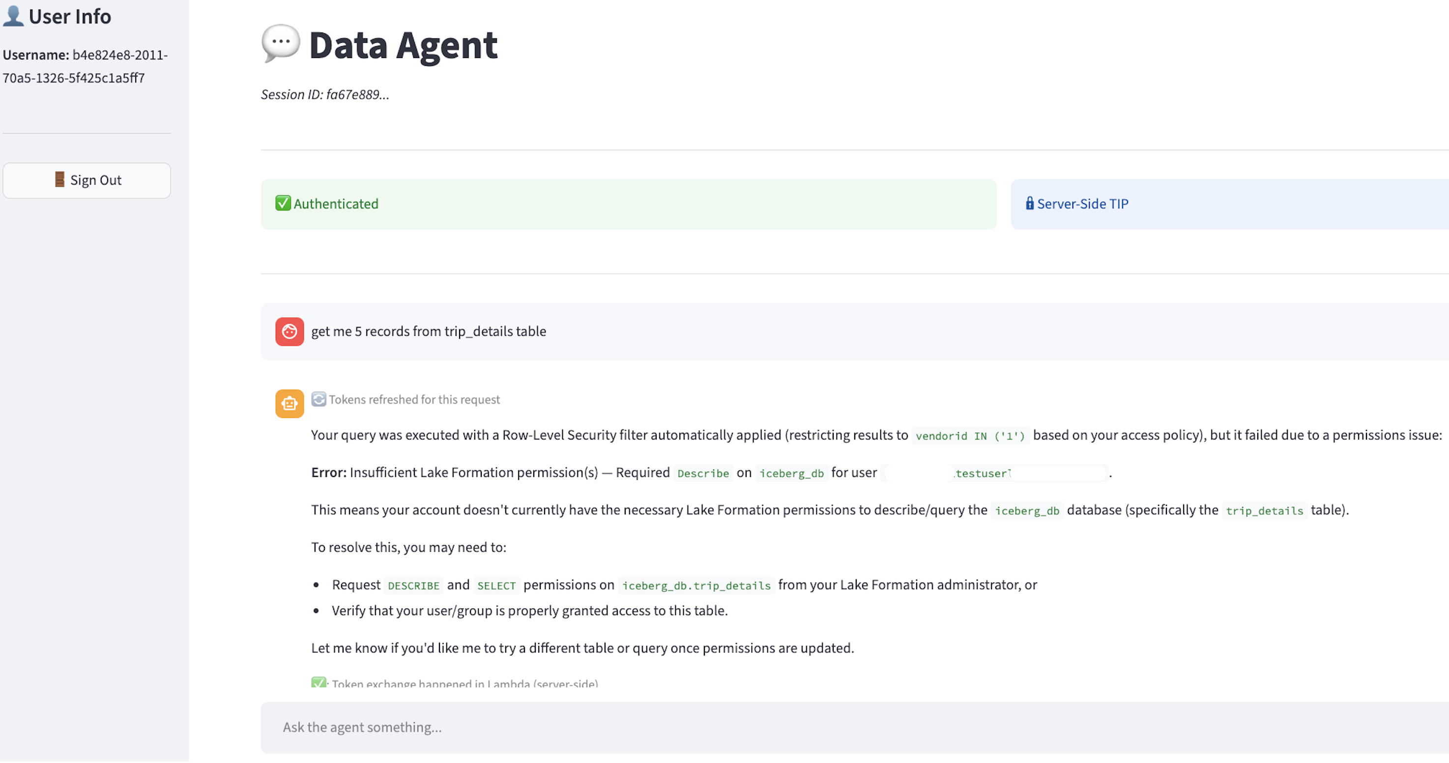
import os
import duckdb

os.makedirs('/tmp/.duckdb/extensions', exist_ok=True)

con = duckdb.connect(':memory:')
con.execute("SET home_directory='/tmp';")
con.execute("SET extension_directory='/tmp/.duckdb/extensions';")

con.execute("INSTALL httpfs; LOAD httpfs;")
con.execute("INSTALL aws; LOAD aws;")
con.execute("INSTALL iceberg; LOAD iceberg;")

con.execute("CREATE SECRET (TYPE s3, PROVIDER credential_chain);")

The home_directory setting must be applied before loading any extensions. Without it, DuckDB attempts to write to /.duckdb/ and fails with IOError: Permission denied.

Step 2: Read and transform with DuckDB SQL

DuckDB reads Amazon S3 Parquet files directly through the httpfs extension. No local download is required. The read_parquet() function accepts Amazon S3 glob patterns, reading multiple files as a single relation.

import sys
from awsglue.utils import getResolvedOptions

args = getResolvedOptions(sys.argv, ['s3_input_path'])
S3_INPUT = args['s3_input_path']

con.execute(f"""
CREATE OR REPLACE TEMP TABLE _batch AS
SELECT date_trunc('day', order_date) AS order_day,
region, category,
COUNT(*) AS total_orders,
SUM(quantity * unit_price) AS gross_revenue,
SUM(CASE WHEN status = 'completed'
THEN quantity * unit_price ELSE 0 END) AS net_revenue,
COUNT(DISTINCT customer_id) AS unique_customers,
ROUND(AVG(quantity * unit_price), 2) AS avg_order_value,
SUM(CASE WHEN quantity * unit_price > 500
THEN 1 ELSE 0 END) AS high_value_orders
FROM read_parquet('{S3_INPUT}')
WHERE status IN ('completed', 'processing')
GROUP BY ALL
ORDER BY order_day DESC, gross_revenue DESC
""")

GROUP BY ALL is a DuckDB SQL extension that groups by every non-aggregate column in the SELECT list. It’s a convenience feature rather than standard SQL, and support varies across query engines. If you adapt this query for another engine, check whether it supports GROUP BY ALL or list the grouping columns explicitly (GROUP BY order_day, region, category).

The WHERE clause retains both completed and processing orders. The gross_revenue column reflects all in-flight revenue, while net_revenue counts only completed orders. A partition containing only processing orders shows net_revenue = 0. This is by design: the two columns serve different reporting purposes.

Step 3: Write to Amazon S3 Tables

DuckDB attaches the S3 Tables bucket as an Iceberg REST catalog using the ENDPOINT_TYPE s3_tables option. DuckDB commits each write as a new Iceberg snapshot through the catalog.
The write uses an idempotent per-day reload pattern: create the table if it does not exist, delete any existing rows for the batch’s date range, then insert. This way, re-runs don’t produce duplicate rows.
Note: The DELETE and INSERT are not committed atomically. If the job fails between them, the affected partition is left empty. For mitigations, see Error handling for production.

import sys
from awsglue.utils import getResolvedOptions

args = getResolvedOptions(sys.argv, ['s3t_arn'])
S3T_ARN = args['s3t_arn']

con.execute(f"ATTACH '{S3T_ARN}' AS s3t (TYPE iceberg, ENDPOINT_TYPE s3_tables);")
con.execute("CREATE SCHEMA IF NOT EXISTS s3t.analytics;")
con.execute("""
CREATE TABLE IF NOT EXISTS s3t.analytics.daily_order_summary (
order_day DATE,
region VARCHAR,
category VARCHAR,
total_orders BIGINT,
gross_revenue DOUBLE,
net_revenue DOUBLE,
unique_customers BIGINT,
avg_order_value DOUBLE,
high_value_orders BIGINT
);
""")

con.execute("""
DELETE FROM s3t.analytics.daily_order_summary
WHERE order_day IN (SELECT DISTINCT order_day FROM _batch);
""")
con.execute("""
INSERT INTO s3t.analytics.daily_order_summary BY NAME
SELECT * FROM _batch;
""")

count = con.execute(
"SELECT COUNT(*) FROM s3t.analytics.daily_order_summary"
).fetchone()[0]
print(f"S3 Tables now holds {count} rows in analytics.daily_order_summary")

The resulting Iceberg table is immediately readable by Amazon Athena, Amazon Redshift, and Amazon EMR through the S3 Tables REST catalog. Amazon S3 Tables handles compaction, snapshot expiration, and orphan-file cleanup automatically.

Complete AWS Glue 6.0 job script

The following script combines all three steps with structured logging, error handling, and AWS Glue job parameter parsing. It can be used directly as the script for an AWS Glue 6.0 glueetl job.

import os, sys, logging, duckdb
from awsglue.utils import getResolvedOptions

logging.basicConfig(level=logging.INFO,
                    format='%(asctime)s %(levelname)s %(message)s')
logger = logging.getLogger(__name__)

TARGET = 's3t.analytics.daily_order_summary'

DDL = """
CREATE TABLE IF NOT EXISTS s3t.analytics.daily_order_summary (
order_day DATE, region VARCHAR, category VARCHAR,
total_orders BIGINT, gross_revenue DOUBLE, net_revenue DOUBLE,
unique_customers BIGINT, avg_order_value DOUBLE, high_value_orders BIGINT
);
"""

TRANSFORM = """
SELECT date_trunc('day', order_date) AS order_day,
region, category,
COUNT(*) AS total_orders,
SUM(quantity * unit_price) AS gross_revenue,
SUM(CASE WHEN status = 'completed' THEN quantity * unit_price ELSE 0 END) AS net_revenue,
COUNT(DISTINCT customer_id) AS unique_customers,
ROUND(AVG(quantity * unit_price), 2) AS avg_order_value,
SUM(CASE WHEN quantity * unit_price > 500 THEN 1 ELSE 0 END) AS high_value_orders
FROM read_parquet('{s3_input}')
WHERE status IN ('completed', 'processing')
GROUP BY ALL
ORDER BY order_day DESC, gross_revenue DESC
"""

def setup_duckdb():
    os.makedirs('/tmp/.duckdb/extensions', exist_ok=True)
    con = duckdb.connect(':memory:')
    con.execute("SET home_directory='/tmp';")
    con.execute("SET extension_directory='/tmp/.duckdb/extensions';")
    con.execute("INSTALL httpfs; LOAD httpfs;")
    con.execute("INSTALL aws; LOAD aws;")
    con.execute("INSTALL iceberg; LOAD iceberg;")
    con.execute("CREATE SECRET (TYPE s3, PROVIDER credential_chain);")
    logger.info("DuckDB %s initialized with httpfs, aws, and iceberg extensions",
                duckdb.__version__)
    return con

def transform_orders(con, s3_path):
    logger.info("Reading source data: %s", s3_path)
    con.execute("CREATE OR REPLACE TEMP TABLE _batch AS " +
                TRANSFORM.format(s3_input=s3_path))
    return con.execute("SELECT COUNT(*) FROM _batch").fetchone()[0]

def write_to_s3_tables(con, s3t_arn):
    con.execute(f"ATTACH '{s3t_arn}' AS s3t (TYPE iceberg, ENDPOINT_TYPE s3_tables);")
    con.execute("CREATE SCHEMA IF NOT EXISTS s3t.analytics;")
    con.execute(DDL)
    con.execute(f"""
DELETE FROM {TARGET}
WHERE order_day IN (SELECT DISTINCT order_day FROM _batch);
""")
    con.execute(f"INSERT INTO {TARGET} BY NAME SELECT * FROM _batch;")
    count = con.execute(f"SELECT COUNT(*) FROM {TARGET}").fetchone()[0]
    logger.info("Write complete. %s now holds %s rows.", TARGET, count)
    return count

def main():
    args = getResolvedOptions(sys.argv, ['s3_input_path', 's3t_arn'])
    con = setup_duckdb()
    n = transform_orders(con, args['s3_input_path'])
    logger.info("Transformed %s summary rows", n)
    total = write_to_s3_tables(con, args['s3t_arn'])
    logger.info("ETL complete. Table holds %s total rows.", total)

if __name__ == '__main__':
    main()

Create the job using the AWS CLI:

aws glue create-job \
    --name duckdb-order-summary \
    --role <YOUR-AWS-GLUE-ROLE> \
    --glue-version "6.0" \
    --number-of-workers 2 --worker-type G.1X \
    --command '{"Name":"glueetl","ScriptLocation":"s3://<amzn-s3-demo-source-bucket>/scripts/duckdb_job.py","PythonVersion":"3"}' \
    --default-arguments '{
    "--additional-python-modules": "duckdb==1.5.1",
    "--s3_input_path": "s3://<YOUR-SOURCE-BUCKET>/orders/year=2026/month=08/*.parquet",
    "--s3t_arn": "arn:aws:s3tables:<YOUR-REGION>:<YOUR-ACCOUNT-ID>:bucket/<amzn-s3-demo-table-bucket>"
}'

Note. Replace the angle-bracket placeholders (<amzn-s3-demo-source-bucket>, <amzn-s3-demo-table-bucket>, <YOUR-REGION>, <YOUR-ACCOUNT-ID>, <YOUR-AWS-GLUE-ROLE>) with your own values before running.

Lake Formation permissions. Amazon S3 Tables access is governed by AWS Lake Formation. Grant the AWS Glue job role only the permissions the job needs: SELECT, INSERT, and DELETE on the target table (daily_order_summary), plus CREATE_TABLE on the analytics namespace so the job can create the table on first run. For the exact permission names and resource scoping, see the Lake Formation permissions reference. The role also requires the lakeformation:GetDataAccess IAM action. Without these grants, the ATTACH and CREATE TABLE statements fail with an access-denied error.

Error handling for production

For production use, plan for three failure modes:

  • Catalog access. If ATTACH to Amazon S3 Tables returns an access-denied error, verify that the IAM role of the job has the scoped Amazon S3 Tables actions on the table bucket ARN and the required AWS Lake Formation grants. Writes need both.
  • Partial writes. The DELETE and INSERT are not committed atomically, so a failure between them can leave a partition empty. Set MaxRetries to 1 so the idempotent reload re-runs automatically, or write to a staging table and swap on success.
  • Timeouts. Set the job Timeout higher than the expected run time to stop hung runs.

Monitoring

DuckDB runs inside a standard AWS Glue job, so you monitor it with the same Amazon CloudWatch metrics as any AWS Glue job. Two are useful for right-sizing this workload:

  • glue.driver.jvm.heap.usage: driver memory pressure. A high or climbing value means the worker needs more memory or the query is spilling heavily to disk.
  • glue.driver.aggregate.bytesRead: bytes read from Amazon S3, useful for correlating input size with runtime and cost.

The internal execution metrics of DuckDB (query plan, operator timings, spill volume) aren’t exposed to Amazon CloudWatch. Structured logging from the job script is the primary way to observe DuckDB itself: the production script uses logger.info to record the rows transformed and rows written, and those lines appear in the CloudWatch Logs stream of the job. Add more logger.info statements around each stage if you need finer-grained timing.

Measured results

The measurements in this section were collected on AWS Glue 6.0 with DuckDB 1.5.1 writing to Amazon S3 Tables in the US East (N. Virginia) Region (us-east-1). Output tables were verified by querying them in Amazon Athena. Both jobs produced identical output: 1,176 summary rows.

The dataset consisted of 8.4 million rows across 12 Parquet files (approximately 94 MB compressed on disk, approximately 1.2 GB uncompressed). One job ran DuckDB on the AWS Glue 6.0 runtime. The other ran Apache Spark on AWS Glue 6.0 with the equivalent transform and a native Iceberg write.

Metric

DuckDB on AWS Glue 6.0

Spark on AWS Glue 6.0

Compute configuration 2 DPU (2x G.1X) 2 DPU (2x G.1X)
Job Duration ~56 seconds ~117 seconds
Billed duration 1 minute (minimum) 2 minutes
Cost per run $0.0103 $0.0205
Output rows (Athena-verified) 1,176 1,176

On the same AWS Glue 6.0 runtime and the same 2 DPU configuration, DuckDB completed in approximately half the time at approximately half the cost of Spark for this workload.

Cost is calculated at $0.308 per DPU-hour (AWS Glue 6.0 rate). AWS Glue bills in 1-second increments with a 1-minute minimum per run. Verify against the current AWS Glue pricing page for your Region. Results scale with dataset size, query complexity, and Region.

At 20 runs per day, this job costs approximately $75 per year with DuckDB, compared to $150 per year with Spark. Beyond the cost savings, this pattern keeps SQL-centric work quick to iterate on: you express the transformation in SQL, and DuckDB runs it in-process on the AWS Glue worker.

Clean up

To avoid ongoing charges, delete the resources created during this walkthrough:

  1. Delete the AWS Glue job (duckdb-order-summary).
  2. Remove the sample data from your Amazon S3 bucket (s3://<amzn-s3-demo-source-bucket>/orders/).
  3. Drop the Iceberg table in Amazon Athena: DROP TABLE analytics.daily_order_summary;
  4. Delete the Amazon S3 Tables table bucket if it was created for this walkthrough.
  5. Revoke the AWS Lake Formation grants and remove the IAM role if no longer needed.

Conclusion

In this post, we demonstrated how to run DuckDB inside an AWS Glue 6.0 job to read Amazon S3 Parquet, transform it with SQL, and write Apache Iceberg tables directly to Amazon S3 Tables. AWS Glue 6.0 modernized the runtime environment to Amazon Linux 2023, Python 3.13, and Apache Spark 4.1. With that modernization, you can run embedded SQL in the AWS Glue job and write Iceberg tables directly to Amazon S3 Tables. For ETL jobs where the data fits in memory on a single worker, this pattern completed the same work in approximately half the time and half the cost of Spark. The Measured results section describes these measurements. The job uses the same glueetl job type, IAM configuration, and triggering mechanisms as any Spark job on AWS Glue. When a workload outgrows single-worker processing, switching the script back to PySpark requires no infrastructure changes. The result is the ability to match the engine to each job: a scheduled SQL transformation and a large distributed workload can run on one platform, and you pick the engine per job without managing separate systems.

To get started, create an AWS Glue 6.0 job, add duckdb==1.5.1 through the --additional-python-modules parameter, and point it at your Amazon S3 source data and an Amazon S3 Tables bucket. The complete script in this post is a working starting point you can adapt to your own datasets and schedules. For more information, see the AWS Glue Developer Guide and the Amazon S3 Tables user guide. For a complementary pattern that uses DuckDB to read and query data in Amazon S3 Tables, see Streamlining access to tabular datasets stored in Amazon S3 Tables with DuckDB.


About the authors

Bezuayehu Wate

Bezuayehu Wate

Bezuayehu is a Specialist Solutions Architect at AWS, specializing in big data analytics and AI. She works closely with customers to modernize their analytics platforms with AWS data and AI services, and is passionate about emerging technologies and designing cloud solutions that deliver measurable impact for customers.

Manjeet Chayel

Manjeet Chayel

Manjeet Chayel serves as Big Data Manager, Worldwide Specialist Solutions Architects at AWS, where he leads a global team of specialist architects driving customer-facing engagements across Amazon EMR, AWS Glue, and the broader Big Data Analytics portfolio. With over 15 years at Amazon, he brings deep expertise in big data processing and building experiences that operate reliably at massive scale combining work with customers architecting their analytics platforms with a focus on scaling and developing the next generation of technical leaders across AWS.

All the numbers: Amazon Prime Day 2026 powered by AWS

Post Syndicated from Channy Yun (윤석찬) original https://aws.amazon.com/blogs/aws/all-the-numbers-amazon-prime-day-2026-powered-by-aws/

Amazon Prime Day 2026 was exclusively for Prime members and ran June 23–26, 2026 with millions of deals across more than 35 categories.

As part of our annual tradition of sharing how AWS powered Prime Day (2016, 2017, 2019, 2020, 2021, 2022, 2023, 2024, and 2025), I want to share the services and chart-topping metrics from AWS that made your amazing shopping experience possible.

Prime Day 2026 – all the numbers

As always, Prime Day was powered by AWS. Here are some of the most interesting and/or mind-blowing metrics:

Amazon Elastic Compute Cloud (Amazon EC2) and AWS Graviton – During Amazon Prime Day 2026, AWS Graviton powered up to 49% of the Amazon EC2 compute used by Amazon.com.

Amazon Elastic Block Store (Amazon EBS) – During Prime Day 2026, Amazon EBS, our high-performance block storage service, peaked at over 24.8 trillion I/O operations, moving over an exabyte of data daily.

AWS Lambda – AWS Lambda handled over 2.3 trillion invocations per day during Prime Day 2026.

Amazon Elastic Container Service (ECS) and Fargate – During Prime Day 2026, Amazon ECS launched an average of 158.3 million tasks per day on AWS Fargate, representing a 47.7 percent increase from the previous year’s Prime Day average.

Amazon CloudFront – Amazon CloudFront delivered over 2.1 trillion HTTP requests during the global week of Prime Day 2026, a 5 percent increase in total requests compared to Prime Day 2025.

Amazon DynamoDB – Amazon DynamoDB, a serverless, fully managed, distributed NoSQL database, powers multiple high-traffic Amazon properties and systems including Alexa, the Amazon.com sites, and all Amazon fulfillment centers. Over the course of Prime Day 2026, between June 23 and June 26, 2026, DynamoDB processed over 59 trillion requests. DynamoDB maintained high availability while delivering single-digit millisecond responses and peaking at 192 million requests per second.

Amazon Aurora – On Prime Day, Amazon Aurora, a relational database management system (RDBMS) built for high performance and availability at global scale for PostgreSQL, MySQL, and DSQL, processed hundreds of billions of transactions, stored 5,491 terabytes of data, and transferred 1,194 terabytes of data.

Amazon ElastiCache – During Prime Day, Amazon ElastiCache peaked at serving over 2.3 quadrillion daily requests and 2.1 trillion requests in a minute.

Amazon Kinesis Data Streams – Amazon Kinesis Data Streams, a fully managed serverless data streaming service, processed a peak of 988 million records per second during Prime Day 2026.

Amazon Simple Notification Service (SNS) – Amazon SNS, a fully managed pub/sub messaging service for application-to-application and application-to-person communication, delivered 5 trillion messages in a single day during Prime Day 2026.

Amazon Simple Queue Service (SQS) – Amazon SQS, a fully managed message queuing service for microservices, distributed systems, and serverless applications, received a peak of 213 million messages per second during Prime Day 2026

AWS CloudTrail – AWS CloudTrail processes billions of API activity events per day for governance, compliance, and operational auditing. During Prime Day 2026, that volume surged to 3.6 trillion events in just four days, a 44% increase over Prime Day 2025.

AWS CloudWatch – Amazon CloudWatch processed over 2.15 quadrillion metric observations per day during Prime Day 2026.

Amazon GuardDuty – During Prime Day 2026, Amazon GuardDuty monitored an average of 14.08 trillion log events per hour, a 59% increase from last year’s Prime Day.

AWS Fault Injection Service (FIS) – We ran over 44,000 AWS FIS experiments – more than six times what we conducted in 2025 – to help ensure Amazon.com remains highly available on Prime Day.

Prepare to scale

If you’re preparing for similar business-critical events, product launches, and migrations, I recommend that you take advantage of AWS Countdown Premium. From retail peak seasons to major sporting events, elections, and healthcare enrollment periods, we help you deliver flawless experiences when it matters most. Our experts help you manage your infrastructure to handle massive traffic spikes while maintaining security and performance. We work alongside your team to scale infrastructure, optimize costs during demand surges, strengthen security measures, and monitor real-time demands. To learn more, visit AWS Countdown Premium for business critical events.

I look forward to seeing what other records will be broken next year!

— Channy

Identity-aware AI data agents with AWS Lake Formation and Trusted Identity Propagation

Post Syndicated from Thiyagarajan Mani original https://aws.amazon.com/blogs/security/identity-aware-ai-data-agents-with-aws-lake-formation-and-trusted-identity-propagation/

You’re building a data agent that lets business users ask questions about lakehouse data in natural language. You’ve already built governance policies that control who can access which datasets. The challenge is making the agent respect those rules without rebuilding them in your application code.

When a user asks a question, the agent maps it to data and constructs a query. The tool runs under its own AWS Identity and Access Management (IAM) role, so AWS Lake Formation sees the tool’s credentials, not the person behind the request. This leaves you with two inadequate options: restrict tool access (limiting self-service analytics) or rebuild access controls in application code (moving governance out of the data layer).

In this post, we show you a different approach: identity-aware AI data agents that propagate each user’s identity through every hop, from the user, through the agent, into the tool, so Lake Formation evaluates the user’s grants. Your application code makes no authorization decisions, existing Lake Formation policies work without modifications, and AWS CloudTrail records the actual person who accessed the data.

In this post, you learn how to:

  • Set up per-user data access controls for AI agents querying your lakehouse without rewriting your existing Lake Formation governance policies by configuring Amazon Bedrock AgentCore to carry each user’s identity through trusted identity propagation (TIP).
  • Ensure auditability and compliance by performing a server-side token exchange inside AWS Lambda that converts the identity token into Lake Formation credentials scoped to the real user, with CloudTrail recording every query.
  • Validate the pattern end-to-end by testing with multiple users and confirming per-user query results and CloudTrail audit evidence.

The building blocks in this post, OAuth 2.0 token delegation, AWS IAM Identity Center, Lake Formation, and Lambda are well-documented individually. The new constraint is that a foundation model (FM) now sits in the middle of the propagation chain. The FM is the agent’s brain, it decides which tools to call and what arguments to pass and anything that enters its context (prompts, tool schemas, arguments) is accessible within that trust boundary. So, the user’s identity token must reach the tool, but it must do so on the HTTP transport layer, bypassing the FM’s reasoning layer entirely. This post demonstrates the three Amazon Bedrock AgentCore configurations that achieve that.

Whether you’re building agents on Strands, LangGraph, or a similar framework, this post gives you a deployable pattern on Amazon Bedrock AgentCore. Security engineers will find the identity-transport and audit properties relevant, and data platform owners will see how existing Lake Formation grants extend to AI workloads with no changes.

Solution overview

With this pattern (shown in Figure 1), your data agent can query Lake Formation governed data with per-user access controls, full CloudTrail audit trails, and no changes to your existing governance policies. Here’s how it works.

  1. Two tokens travel through the system. An access_token authenticates the request at each trust boundary (Bedrock AgentCore Runtime, Bedrock AgentCore Gateway). An id_token carries your identity and is exchanged, server-side, for the identity context that Lake Formation evaluates.
  2. A separate TIP role carries only the IAM permissions needed to call service APIs, it has no Lake Formation data grants.
  3. Lake Formation evaluates only the propagated user identity, not the TIP role.

The request flow is:

  1. User to UI: The user authenticates with an OpenID Connect (OIDC) identity provider (IdP). This post uses Amazon Cognito, but you can use any OIDC provider, such as Okta. The UI receives an id_token and an access_token.
  2. UI to Bedrock AgentCore Runtime: The UI calls the agent running in AgentCore Runtime over HTTPS. The access_token goes in the standard Authorization header. The id_token goes in a custom header: X-Amzn-Bedrock-AgentCore-Runtime-Custom-IdToken. The HTTP body contains only the user’s prompt.
  3. AgentCore Runtime to agent code: The runtime validates the access_token against the configured JSON Web Token (JWT) authorizer, then passes the request to the agent container with both headers accessible through context.request_headers.
  4. Agent to Bedrock AgentCore Gateway: The agent opens a Model Context Protocol (MCP) connection to an AgentCore gateway, including both headers on the connection. The AgentCore gateway validates the access_token and forwards the custom header to its Lambda target.
  5. AgentCore Gateway to Lambda: The propagated headers arrive in context.client_context.custom[‘bedrockAgentCorePropagatedHeaders’].
  6. Lambda to the data layer: Lambda validates the id_token, exchanges it for an identity context, assumes a role with that context, and runs the Amazon Athena query under the user’s identity.

Lake Formation evaluates grants against the real user. Athena returns only the rows and columns that the user is entitled to see. CloudTrail records the assumed role with an onBehalfOf entry identifying the human.

Now that you’ve seen the end-to-end flow, the following sections walk through each piece, starting with what you need to have in place before you build.

Prerequisites

This post assumes you have the working knowledge of OAuth 2.0, IAM, and Lake Formation grants.

  • An IAM Identity Center instance with a trusted token issuer (TTI) configured to accept your OIDC IdP’s tokens.
  • An OAuth Application in IAM Identity Center configured for CreateTokenWithIAM with the JWT Bearer grant.
  • Lake Formation governing your AWS Glue Data Catalog, with grants already assigned to users or groups.
  • An Athena workgroup and an Amazon Simple Storage Service (Amazon S3) bucket for query results.
  • An OIDC IdP. The reference implementation uses Amazon Cognito as the demo IdP, but the pattern is IdP-agnostic. Auth0, Microsoft Entra ID, Okta, Ping, or any OIDC-compliant provider works identically, if your TTI accepts its tokens.

This post doesn’t walk through setting up any of these components. The existing AWS documentation covers each one. For more information, see the links in the preceding list and the related resources at the end of this post.

The three Bedrock AgentCore configuration steps

Three Bedrock AgentCore features make this pattern work. Together they form the chain of custody for the user’s id_token from the moment it arrives at the Bedrock AgentCore Runtime to the moment Lambda uses it.

Configure the runtime request header allow list

Bedrock AgentCore Runtime doesn’t pass request headers into the agent container by default. You opt in by declaring an allow list, either through agentcore configure or directly in the runtime configuration:

# .bedrock_agentcore.yaml

request_header_configuration:
	requestHeaderAllowlist:
		- Authorization
		- X-Amzn-Bedrock-AgentCore-Runtime-Custom-IdToken

AgentCore Runtime supports two types of forwarded headers:

  • The standard Authorization header for OAuth inbound JWT authentication (access_token), and
  • Custom headers prefixed with X-Amzn-Bedrock-AgentCore-Runtime-Custom-

The id_token in this pattern uses a custom header. Inside the agent, the allow listed headers arrive as a dictionary object on the request context.

The following Python code runs in the agent container:

from bedrock_agentcore.runtime import BedrockAgentCoreApp
 
ID_TOKEN_HEADER = "X-Amzn-Bedrock-AgentCore-Runtime-Custom-IdToken"
app = BedrockAgentCoreApp()
 
@app.entrypoint
def invoke(payload, context):
    request_headers = getattr(context, "request_headers", None) or {}
 
    id_token = ""
    access_token = ""
    for key, value in request_headers.items():
        if key.lower() == ID_TOKEN_HEADER.lower():
            id_token = value
        elif key.lower() == "authorization":
            access_token = value.replace("Bearer ", "")
 
    # ... build MCP headers and call the Gateway

The agent code reads the id_token from the HTTP transport and forwards it (also on the HTTP transport) to the next hop. It doesn’t treat the token as a tool argument and doesn’t inject it into a prompt.

Key takeaway: The runtime allow list is the first gate. Without it, the id_token doesn’t reach your agent code.

Configure AgentCore Gateway metadata for header propagation

An AgentCore Gateway is the Model Context Protocol (MCP) endpoint the agent talks to. When AgentCore Gateway invokes a Lambda target, it doesn’t forward arbitrary request headers by default. You configure which headers to propagate using metadataConfiguration.allowedRequestHeaders on the target:

from aws_cdk import aws_bedrockagentcore as agentcore
 
self.gateway_target = agentcore.CfnGatewayTarget(
    self, "AthenaTarget",
    name="athena-executor",
    gateway_identifier=self.gateway.attr_gateway_identifier,
    target_configuration=agentcore.CfnGatewayTarget.TargetConfigurationProperty(
        mcp=agentcore.CfnGatewayTarget.McpTargetConfigurationProperty(
            lambda_=agentcore.CfnGatewayTarget.McpLambdaTargetConfigurationProperty(
                lambda_arn=lambda_function_arn,
                tool_schema=...  # execute_athena_query
            ),
        ),
    ),
    metadata_configuration=agentcore.CfnGatewayTarget.MetadataConfigurationProperty(
        allowed_request_headers=["X-Amzn-Bedrock-AgentCore-Runtime-Custom-IdToken"],
    ),
    ...
)

Notice that the tool schema doesn’t include an id_token parameter; there’s no token parameter on any tool. The FM doesn’t see, select, or pass an id_token because the token isn’t part of the tool’s contract. It travels parallel to the tool call, on the HTTP connection, through metadataConfiguration.

This is a critical property for security. If you put the id_token in the tool schema instead, the FM becomes responsible for passing it, which means the token lands in prompts, traces, memory, and logs. Keeping the token off the tool contract keeps it out of the FM entirely.

Key takeaway: The metadataConfiguration of the AgentCore gateway is the second gate. It controls which headers cross from the agent into the Lambda function without touching the tool schema.

Read propagated headers in Lambda

On the Lambda side, the propagated header arrives not in the event body but in the client context, under a specific key.

The following Python code runs in the Lambda function:

ID_TOKEN_HEADER = "X-Amzn-Bedrock-AgentCore-Runtime-Custom-IdToken"
 
def lambda_handler(event, context):
    client_ctx = getattr(context.client_context, "custom", {}) or {}
    propagated_headers = client_ctx.get("bedrockAgentCorePropagatedHeaders", {})
    id_token = propagated_headers.get(ID_TOKEN_HEADER)
 
    if not id_token:
        return {"statusCode": 400, "body": {"error": "missing id_token"}}
 
    # Tool arguments from the agent's call (no id_token here)
    query = event["query"]
    database = event["database"]
    workgroup = event["workgroup"]
    output_location = event["output_location"]
 
    # ... validate token, exchange, run query

The event dictionary contains the tool’s declared parameters and nothing else. You reach the id_token only through context.client_context.custom[‘bedrockAgentCorePropagatedHeaders’]. That’s the handoff point.

Key takeaway: The id_token arrives through the client context rather than tool arguments; the FM has no access to it. The Lambda is the only component that reads the token.

Perform the server-side token exchange

After Lambda has the id_token, it validates the token and exchanges it for an identityContext. This step uses standard IAM Identity Center TIP mechanics. That it happens inside Lambda rather than anywhere else is what keeps the identity context from crossing a process boundary.

import boto3, jwt, time
 
def exchange_and_assume(id_token: str, user_sub: str):
    # 1. Validate id_token against the OIDC IdP's JWKS.
    claims = validate_id_token(id_token)  # signature, exp, aud, iss, token_use
 
    # 2. Exchange for an Identity Center identityContext.
    sso_oidc = boto3.client("sso-oidc")
    resp = sso_oidc.create_token_with_iam(
        clientId=OAUTH_APPLICATION_ARN,
        grantType="urn:ietf:params:oauth:grant-type:jwt-bearer",
        assertion=id_token,
    )
    identity_context = resp["awsAdditionalDetails"]["identityContext"]
 
    # 3. AssumeRole with ProvidedContexts
    sts = boto3.client("sts")
    assumed = sts.assume_role(
        RoleArn=TIP_ROLE_ARN,
        RoleSessionName=f"agent-tip-{user_sub[:8]}-{int(time.time())}",
        ProvidedContexts=[{
            "ProviderArn": "arn:aws:iam::aws:contextProvider/IdentityCenter",
            "ContextAssertion": identity_context,
        }],
    )
    creds = assumed["Credentials"]
    return boto3.Session(
        aws_access_key_id=creds["AccessKeyId"],
        aws_secret_access_key=creds["SecretAccessKey"],
        aws_session_token=creds["SessionToken"],
    )

Two properties come out of this exchange:

  • The identityContext is created and consumed inside a single Lambda invocation. It doesn’t get returned to the agent, the gateway, or the UI.
  • The resulting boto3.Session holds short-lived credentials whose underlying identity assertion is the real user. When the session calls Athena, the query runs with the user’s identity propagated. Lake Formation sees the user, not the Lambda function’s role.

Everything after this, including the Athena query and result formatting, is standard boto3.

Configure Lake Formation grants

You need one grant to the IAM Identity Center user or group. That’s the whole story at the Lake Formation layer.

aws lakeformation grant-permissions \
  --principal DataLakePrincipalIdentifier=arn:aws:identitystore:::user/<USER_ID> \
  --resource '{"Table":{"DatabaseName":"iceberg_db","Name":"trip_details"}}' \
  --permissions SELECT

This is the grant Lake Formation evaluates at query time. You add column-level and row-level filters to the same user or group the same way. Nothing here is aware of or specific to AI agents. If you already have a Lake Formation grants model for human users, you already have the grants this pattern needs.

Understanding the TIP role: The TIP role that Lambda assumes has no Lake Formation data grants. It holds only IAM permissions to call the service APIs: athena:* for query runs, glue:* for catalog reads, lakeformation:GetDataAccess for the query plan handshake, and Amazon S3 access for the Athena output bucket. When Lambda assumes this role with an identityContext attached through ProvidedContexts, Lake Formation evaluates only the propagated user identity against its grants. The role itself is transparent to the authorization decision.

In the more common agent runs as a role pattern, the role carries the grants, which is why per-user governance breaks. Here the role carries no grants; it’s a session vehicle, not an authorization subject.

Test the pattern end-to-end

Two users, same question, different outcomes.

User A has SELECT on trip_details. They ask the agent for five records from the table.

Figure 2: Five records are requested and returned by the agent

Figure 2: Five records are requested and returned by the agent

User B has no grant on trip_details. They ask the same question.

Figure 3: User doesn’t have access to the data

Figure 3: User doesn’t have access to the data

No code changed between the two interactions. No parameter was toggled. Lake Formation made the decision based on the propagated identity.

The CloudTrail record for the AssumeRole call shows the delegation:

{
  "eventSource": "sts.amazonaws.com",
  "eventName": "AssumeRole",
  "requestParameters": {
    "roleArn": "arn:aws:iam::<ACCOUNT_ID>:role/<TIP_ROLE_NAME>",
    "roleSessionName": "agent-tip-<user_sub_prefix>-<timestamp>",
    "providedContexts": [{
      "providerArn": "arn:aws:iam::aws:contextProvider/IdentityCenter",
      "contextAssertion": "<identity-context-assertion>"
    }]
  },
  "userIdentity": {
    "type": "AssumedRole",
    "onBehalfOf": {
      "userId": "<IDENTITY_STORE_USER_ID>",
      "identityStoreArn": "arn:aws:identitystore::<ACCOUNT_ID>:identitystore/<ID>"
    }
  }
}

The onBehalfOf block closes the audit loop. Each query the agent runs on a user’s behalf has a CloudTrail record naming that user, with no additional instrumentation in your code.

Security properties

Four properties follow from this architecture. These are the core value propositions of the identity-aware pattern:

  1. The id_token never reaches the foundation model: It travels on HTTP headers at every hop, and Lambda reads it from context.client_context.custom. It’s not a parameter on any tool. The FM has no path to it: not in tool arguments, not in prompts, not in memory, not in traces.
  2. The identity context stays inside a single Lambda invocation: It’s derived from the id_token, used immediately in an AssumeRole call, and discarded. It doesn’t go back to the agent, the gateway, or the UI.
  3. Authorization decisions live in Lake Formation, against the real user only: The TIP role the Lambda function assumes has no data grants. Lake Formation evaluates the propagated user identity. No code path in the agent, gateway, or Lambda function performs authorization logic.
  4. The audit trail requires no extra work: The CloudTrail AssumeRole event with onBehalfOf identifies the human user for every query. You get the same audit fidelity you would have for human users accessing data directly.

Deploy the pattern

To deploy this pattern, you need to configure four things:

  1. An OIDC IdP with a TTI in IAM Identity Center accepting its tokens, and an Identity Center OAuth Application configured for CreateTokenWithIAM.
  2. Bedrock AgentCore Runtime running your agent container with requestHeaderAllowlist covering Authorization and your custom id_token header.
  3. Bedrock AgentCore Gateway with a Lambda target whose metadataConfiguration.allowedRequestHeaders includes the id_token header. The Lambda target’s tool schema has no id_token parameter.
  4. Lambda reading the id_token from context.client_context.custom[‘bedrockAgentCorePropagatedHeaders’], performing the token exchange through sso-oidc:CreateTokenWithIAM, and calling sts:AssumeRole with ProvidedContexts to get the TIP-bearing session.

Conclusion

When an AI agent queries a governed lakehouse, the data layer needs to know who’s asking, not which role the agent is running under. This post showed you how to resolve that by treating the agent as an OAuth delegated actor. The user’s token travels alongside the agent’s HTTP transport but doesn’t enter the model’s context, and the token exchange that produces query-time credentials happens server-side inside Lambda, scoped to a single invocation.

The three Bedrock AgentCore features that make this composable (requestHeaderAllowlist on runtime, metadataConfiguration.allowedRequestHeaders on gateway, and bedrockAgentCorePropagatedHeaders on Lambda) are specific to building on Bedrock AgentCore. Everything downstream of Lambda is IAM Identity Center and Lake Formation functionality.

If you’re building agents that read governed data, you don’t have to choose between a single over-permissioned service role and per-user code paths. The identity the data layer evaluates can be the real user, the audit trail can name the real user, and the foundation model doesn’t need to know the user’s token exists.

The result is a clean separation: the user’s identity travels end-to-end, the model never sees it, and the data layer enforces it exactly as if the user queried directly.

Related resources

If you have feedback about this post, submit comments in the Comments section below.


Thiyagarajan Mani

Thiyagarajan Mani

Thiyagarajan is a Sr. Delivery Consultant at AWS. With over 20 years of experience, he architects modern data platforms spanning lakehouses, ingestion pipelines, and generative and agentic AI applications. He specializes in transforming legacy data ecosystems into scalable, cloud-centered architectures that unlock advanced analytics and intelligent automation for customers. Outside work, he enjoys time with family and riding bikes.

Mihir Borkar

Mihir Borkar

Mihir is a Senior Solutions Architect at AWS, partnering with ISVs to build and scale their platforms. With a decade of experience across data architecture and delivery, his background in enterprise-scale engagements gives him a builder’s perspective, bridging architecture strategy with practical implementation. Outside work, he explores the latest developments in cloud technologies and AI/ML.

Philippe-Duplessis-Guindon

Philippe Duplessis-Guindon

Philippe is a Delivery Consultant at AWS, where he has worked on a wide range of generative AI projects, touching on most aspects from infrastructure and DevOps to software development and AI/ML. After earning his bachelor’s in software engineering and a master’s in computer vision and machine learning from Polytechnique Montréal, he joined AWS to help customers accelerate their generative AI journeys.

Umang Khambhalikar

Umang Khambhalikar

Umang is a Senior Consultant at AWS Professional Services, specializing in data and AI. He helps enterprise customers design and implement secure, governed data platforms and agentic AI solutions using services like Amazon Bedrock AgentCore, AWS Lake Formation, and AWS Glue. Umang brings over 19 years of IT consulting experience to solving complex challenges at the intersection of security, data governance, and generative AI.

Query across accounts and table formats with multi-catalog in Amazon EMR

Post Syndicated from Suthan Phillips original https://aws.amazon.com/blogs/big-data/query-across-accounts-and-table-formats-with-multi-catalog-in-amazon-emr/

Analytics teams on AWS often store data in more than one open table format, and that data frequently lives in more than one AWS account. Two problems follow: querying across table formats without catalog-level complexity, and joining data across accounts without copying it. This is common in a data mesh, where domain teams own data in separate AWS accounts while analytics workloads run centrally. Multi-catalog support in Amazon EMR 8.1.0 addresses both problems.

Amazon EMR release 8.1.0 addresses both challenges with multi-catalog support. The RedirectingSessionCatalog (RSC) is an opt-in catalog that you set as the Spark default. It automatically detects each table’s format from AWS Glue metadata, routes queries to the correct format handler, and supports multiple AWS Glue Data Catalogs across AWS accounts. With multi-catalog support, you can query Iceberg, Hudi, Delta Lake, and Hive tables through a single unified catalog. You can also join tables across AWS accounts without copying data and discover remote catalogs dynamically at query time.

In this post, we show how to put these capabilities into practice using Amazon EMR Serverless.

The Spark single-catalog constraint

Many formats. The Spark default catalog (spark_catalog) accepts only one CatalogExtension at a time: SparkSessionCatalog for Iceberg, DeltaCatalog for Delta Lake, or HoodieCatalog for Hudi. You configure one, and queries against tables in other formats fail unless those tables are registered in a separate, format-specific catalog.

Many accounts. The Spark V1 metastore (ExternalCatalog) is a singleton bound to one AWS Glue Data Catalog in one account. The Spark V2 catalog API supports named catalogs, but only Iceberg uses it. Delta Lake, Hudi, and Hive tables still rely on V1. As a result, cross-account access for those formats required complex multi-step workarounds. These included AWS Lake Formation grants, AWS Resource Access Manager (AWS RAM) shares, resource links, and per-table permissions.

Amazon EMR 8.1.0 addresses both constraints with the RedirectingSessionCatalog, described in the following section.

The RedirectingSessionCatalog

The RedirectingSessionCatalog provides three opt-in, backward-compatible capabilities. Set RSC as the default catalog to run multi-format queries without format-specific prefixes. Declare a named RSC catalog to join across accounts without data copies. Turn on the AWS Glue Data Catalog resolver to discover and register remote catalogs at query time, with no upfront spark.sql.catalog.* configuration. The following sections cover each capability.

Multi-format support

In Amazon EMR 8.1.0, you set the default catalog to the RedirectingSessionCatalog (RSC). On table resolution, RSC calls the AWS Glue Data Catalog, reads the table’s format from its metadata, caches the result, and delegates to the matching format-specific catalog (Iceberg, Delta Lake, Hudi, or Hive).

Without this feature, you had to register a separate catalog for each format and prefix every table reference:

# One catalog per format, all pointing at the same Glue metastore
spark.sql.catalog.spark_catalog = org.apache.iceberg.spark.SparkSessionCatalog
spark.sql.catalog.delta_catalog = org.apache.spark.sql.delta.catalog.DeltaCatalog
spark.sql.catalog.hudi_catalog = org.apache.spark.sql.hudi.catalog.HoodieCatalog

# Queries must use format-specific catalog prefixes
SELECT * FROM spark_catalog.db.iceberg_table;
SELECT * FROM delta_catalog.db.delta_table;
SELECT * FROM hudi_catalog.db.hudi_table;

With multi-format support, this reduces to a single catalog property:

What you set:

# Replace the default catalog with RedirectingSessionCatalog.
# RSC auto-detects each table's format from Glue metadata.
spark.sql.catalog.spark_catalog = org.apache.spark.sql.connector.catalog.\
redirecting.RedirectingSessionCatalog

How you query:

-- No format prefixes needed. RSC resolves the format at query time.
SELECT * FROM db.iceberg_table;
SELECT * FROM db.delta_table;
SELECT * FROM db.hudi_table;

-- Cross-format joins work in a single statement.
SELECT i.id, d.val, h.val
FROM db.iceberg_table i
JOIN db.delta_table d ON i.id = d.id
JOIN db.hudi_table h ON i.id = h.id;

On table resolution, RSC:

  • Calls the AWS Glue Data Catalog to read table metadata.
  • Inspects the table’s Parameters map to determine the format (Iceberg, Delta Lake, Hudi, or Hive/Parquet).
  • Delegates the operation to the appropriate format-specific catalog implementation.

The following diagram shows how a single query flows through the RedirectingSessionCatalog to the correct format handler.

RedirectingSessionCatalog routing a query to Iceberg, Delta Lake, Hudi, and Hive handlers through AWS Glue

Figure 1: Multi-format routing. A single query enters the RedirectingSessionCatalog, which calls the AWS Glue Data Catalog to read each table’s format, then routes the table to the matching format-specific handler (Iceberg, Delta Lake, Hudi, or Hive) so results return through one catalog

As the diagram illustrates, the query enters through spark_catalog (the RSC). The RSC reads each table’s format from the AWS Glue Data Catalog and routes the operation to the matching engine: Iceberg, Delta Lake, Hudi, or Hive/Parquet. The four format handlers read the underlying data files from Amazon Simple Storage Service (Amazon S3). The caller issues one query with no format-specific catalog prefixes.

Multi-catalog: Cross-account access

When production data lives in a separate AWS account from your analytics compute, you can declare a named RSC catalog that points at that account’s AWS Glue Data Catalog. RSC resolves tables in the remote account the same way it resolves local tables, so a single query can join across accounts without copying data.

Previously, cross-account table resolution worked only for Iceberg (V2 catalog). Hive, Delta Lake, and Hudi tables in another account required manual Lake Formation and AWS RAM configuration rather than catalog-level resolution. With Amazon EMR 8.1.0, you declare a named RSC catalog for the remote account:

Configuration:

# Declare a named catalog pointing at the remote account's Glue catalog.
# "prod" is any name you choose for this catalog.
spark.sql.catalog.prod = org.apache.spark.sql.connector.catalog.\
redirecting.RedirectingSessionCatalog

# Tell it to use Glue as the metastore backend.
spark.sql.catalog.prod.metastore.type = glue

# Point it at the remote account's Glue catalog ID.
spark.sql.catalog.prod.metastore.hadoop.hive.metastore.glue.catalogid = 111122223333

Query:

-- Join local and remote tables directly. No data copy.
SELECT o.order_id, f.status
FROM spark_catalog.analytics.orders o -- local Iceberg table
JOIN prod.salesdb.fulfillment f -- remote Hudi table (account 111122223333)
ON o.order_id = f.order_id;

Each named RSC instance creates its own V1 metastore delegate and registers it with the global SessionCatalog, removing the singleton limitation.

The following diagram shows how a single query joins tables across two AWS accounts through named catalogs.

A query joining a local table and a remote table across two AWS accounts through named catalogs

Figure 2: Cross-account access. A query in the local account references a named RSC catalog that points at a second account’s AWS Glue Data Catalog, so the local and remote tables join in one query without copying data between accounts

As the diagram illustrates, the analytics account uses spark_catalog (the RSC) for its local Glue Data Catalog, while a named catalog (prod) points at the production account’s Glue Data Catalog. The query joins a local table to a remote table in a single statement, shown by the JOIN between the two accounts. Each account keeps its own Glue Data Catalog, and no data is copied between them.

Auto-wiring

The preceding multi-catalog setup requires you to pre-declare each remote catalog in spark.sql.catalog.* properties. Auto-wiring in Amazon EMR 8.1.0 removes this requirement at two levels.

Before Amazon EMR 8.1.0, you declared the resolver, a handler per format, and each handler’s delegate class explicitly:

# Declare the resolver, a per-format handler, and each handler's delegate catalog
spark.sql.catalog.spark_catalog.table-format-resolver = \
com.amazonaws.glue.catalog.redirecting.GlueTableFormatResolver
spark.sql.catalog.spark_catalog.handler.iceberg = \
org.apache.spark.sql.connector.catalog.redirecting.DefaultTableFormatCatalogHandler
spark.sql.catalog.spark_catalog.handler.delta = \
org.apache.spark.sql.connector.catalog.redirecting.DefaultTableFormatCatalogHandler
spark.sql.catalog.spark_catalog.handler.hudi = \
org.apache.spark.sql.connector.catalog.redirecting.DefaultTableFormatCatalogHandler
spark.sql.catalog.spark_catalog.iceberg.delegate-class = org.apache.iceberg.spark.SparkCatalog
spark.sql.catalog.spark_catalog.iceberg.catalog-impl = org.apache.iceberg.aws.glue.GlueCatalog
spark.sql.catalog.spark_catalog.delta.delegate-class = \
org.apache.spark.sql.delta.catalog.DeltaCatalog
spark.sql.catalog.spark_catalog.hudi.delegate-class = \
org.apache.spark.sql.hudi.catalog.HoodieCatalog

# Manually declare every remote catalog you might query
spark.sql.catalog.prod = ...RedirectingSessionCatalog
spark.sql.catalog.prod.metastore.type = glue
spark.sql.catalog.prod.metastore.hadoop.hive.metastore.glue.catalogid = 111122223333
spark.sql.catalog.staging = ...RedirectingSessionCatalog
spark.sql.catalog.staging.metastore.type = glue
spark.sql.catalog.staging.metastore.hadoop.hive.metastore.glue.catalogid = 444455556666

Auto-wiring reduces this to:

Configuration:

# Set the default catalog. EMR auto-registers Iceberg, Delta, Hudi handlers.
# No handler.* properties needed.
spark.sql.catalog.spark_catalog = org.apache.spark.sql.connector.catalog.\
redirecting.RedirectingSessionCatalog

# Enable catalog discovery. The resolver inspects the connection type and
# registers the catalog at query time, with no upfront spark.sql.catalog.* config.
spark.sql.catalogResolver = com.amazonaws.glue.catalog.\
redirecting.GlueCatalogResolver

# Optional. Falls back to the SDK default region chain. Set this to query Glue catalogs in a specific region.
spark.sql.catalogResolver.region = us-east-1

Query:

-- Reference a remote catalog by its account ID. No prior declaration exists.
-- EMR calls Glue GetCatalog, determines the type, registers it on the spot.
SELECT o.order_id, f.status
FROM spark_catalog.analytics.orders o
JOIN `111122223333`.sales.fulfillment f
ON o.order_id = f.order_id;

The AWS Glue Data Catalog resolver is opt-in. When enabled, Amazon EMR issues an AWS Glue GetCatalog API call each time a query references a catalog that hasn’t been registered. This isn’t enabled by default to avoid unintended API calls for catalog names that don’t exist.

At the handler level, setting the default catalog to RedirectingSessionCatalog is enough. Amazon EMR fills in the Iceberg, Delta, and Hudi handlers automatically, so you don’t need to write handler.* properties.

At the catalog level, when you enable the Glue catalog resolver, Amazon EMR discovers new catalogs on demand. The first time a query references an undeclared catalog, Amazon EMR calls the AWS Glue GetCatalog API, inspects the connection type, and registers the catalog at query time.

Dynamic discovery is functional in Amazon EMR 8.1.0 for three catalog types. For standard cross-account AWS Glue catalogs, the resolver registers a redirecting catalog and multi-format routing applies. For Amazon S3 Tables, a capability of Amazon S3, the resolver reads the federated AWS Glue metadata and routes through Iceberg for both reads and writes. It also supports Amazon Redshift Managed Storage.

The following diagram shows how the GlueCatalogResolver discovers and registers a catalog the first time a query references it.

GlueCatalogResolver registering an undeclared catalog at query time through the AWS Glue GetCatalog API

Figure 3: Auto-wiring. When a query references an undeclared catalog, the Glue catalog resolver calls the AWS Glue GetCatalog API, inspects the connection type, and registers the catalog at query time, so no upfront catalog configuration is required

As the diagram illustrates, a query references a catalog that has not been declared, which raises a catalog-not-found condition. The GlueCatalogResolver intercepts it and calls the AWS Glue Data Catalog through the GetCatalog API. Based on the connection type, the resolver registers the appropriate catalog: a redirecting catalog for a cross-account AWS Glue Data Catalog, a push-down catalog for Redshift Managed Storage, or a Spark catalog for Amazon S3 Tables. Registration happens at query time, with no upfront configuration.

Quick start

Follow these steps to enable multi-catalog support on an existing Amazon EMR 8.1.0 application:

1. Set spark_catalog to the RedirectingSessionCatalog:

spark.sql.catalog.spark_catalog = org.apache.spark.sql.connector.catalog.\
redirecting.RedirectingSessionCatalog

Note: If using Delta Lake or Hudi, also add open table format (OTF) session extensions. Hudi additionally requires KryoSerializer.

Note: To query a different AWS account, add a named catalog pointing to that account’s AWS Glue Data Catalog.

2. (Optional) Enable the Glue catalog resolver:

spark.sql.catalogResolver = com.amazonaws.glue.catalog.\
redirecting.GlueCatalogResolver

Step 1 is all you need for Iceberg-only multi-format queries. The notes call out additional configuration for Delta Lake, Hudi, or cross-account scenarios. Step 2 removes the need to pre-declare catalogs by resolving them at query time.

Try it yourself

The following walkthrough creates four tables (one per format), runs a cross-format join, and extends to a cross-account query. The accompanying sample scripts handle resource creation, job submission, and cleanup. The accompanying code is in the aws-emr-utilities repository.

Prerequisites

  • An AWS account with permissions for Amazon EMR Serverless, AWS Glue Data Catalog, and Amazon S3.
  • An Amazon EMR Serverless application running release emr-spark-8.1.0 (Spark). The multi-catalog features also work on Amazon EMR on EC2 and Amazon EMR on EKS.
  • An Amazon EMR Serverless job execution role scoped to the specific AWS Glue databases and S3 prefixes.
  • An S3 bucket for scripts and output (this post uses s3://amzn-s3-demo-bucket/multicatalog/).
  • (For cross-account) A producer account with Lake Formation grants, AWS Glue resource policy, Amazon S3 bucket policy, and AWS Key Management Service (AWS KMS) key policy configured.

Step-by-step implementation

Step 1: Clone the repository and configure

git clone https://github.com/aws-samples/aws-emr-utilities.git
cd aws-emr-utilities/examples/emr-multi-catalog
cp env.template .env
# Edit .env with your application ID, role ARN, bucket, and region

The repository contains two phases: single-account multi-format and cross-account. The .env file stores resource identifiers referenced by all scripts.

Step 2: Bootstrap the environment

./scripts/bootstrap.sh

This script creates the AWS Glue database, uploads PySpark scripts to S3, and verifies that your Amazon EMR Serverless application is in CREATED state. Note the application ID from the output if you have not set it in .env.

Step 3: Create tables across four formats

./scripts/run_demo.sh --phase setup

The setup phase submits a PySpark job that creates one table per format (Iceberg, Delta Lake, Hudi, Hive/Parquet) in a single AWS Glue database with a shared id/val schema. Each CREATE TABLE uses a different USING clause but all go through the same spark_catalog. RSC routes each to the correct engine.

The job configuration includes the RedirectingSessionCatalog, OTF session extensions for Delta and Hudi, and KryoSerializer for Hudi. If your workload is Iceberg-only, you can omit the extensions and serializer.

Step 4: Run the cross-format join

./scripts/run_demo.sh --phase query

This submits a query that references four tables by database.table only, with no format prefix. The query joins all four through a single catalog with no format-specific configuration:

SELECT i.id, i.val AS iceberg, d.val AS delta, h.val AS hudi, p.val AS hive
FROM salesdb.orders_iceberg i
JOIN salesdb.returns_delta d ON i.id = d.id
JOIN salesdb.shipments_hudi h ON i.id = h.id
JOIN salesdb.products_hive p ON i.id = p.id;

Expected output:

+---+---------+-------+-------+------+
| id| iceberg | delta | hudi | hive |
+---+---------+-------+-------+------+
| 1| ice-1 | dl-1 | hu-1 | hv-1 |
| 2| ice-2 | dl-2 | hu-2 | hv-2 |
| 3| ice-3 | dl-3 | hu-3 | hv-3 |
+---+---------+-------+-------+------+

Each column came from a different table format, joined in one query with no format-specific catalog configuration.

Step 5: (Optional) Extend to cross-account

Cross-account access requires grants from the account that owns the data. Run one bootstrap in each account:

# In the consumer account (where EMR runs):
./scripts/bootstrap_consumer.sh --region us-east-1 \
--producer-account 111122223333

# In the producer account (which owns the data):
./scripts/bootstrap_producer.sh \
--consumer-role <ROLE_ARN from previous step>

Then, back in the consumer account, run the cross-account phase:

./scripts/run_demo.sh --phase xacct-autowire \
--producer-account 111122223333 --producer-table fulfillment

The result joins the producer account’s table to a local Iceberg table in a single query, with no data copy.

For the full cross-account policy setup (Lake Formation grants, AWS Glue resource policy, S3 bucket policy, and AWS KMS key policy), see the Cross-account setup section.

Tip: Add –dry-run to either bootstrap script to preview every action it would take (buckets, roles, policies, applications) without creating anything.

Clean up

To avoid ongoing charges, run the clean-up script or follow the steps in the repository README:

./scripts/cleanup.sh

This removes S3 data, AWS Glue databases and tables, Lake Formation permissions, and the Amazon EMR Serverless application.

Cross-account setup

Cross-account access requires configuration across four services. The following example shows the AWS Glue resource policy. The accompanying bootstrap_producer.sh script configures all four, so you don’t need to author each policy by hand.

1. AWS Lake Formation: Grant permissions on the database and tables to the consumer principal.

2. AWS Glue resource policy: Allow cross-account access to catalog metadata.

3. Amazon S3 bucket policy: Allow access to the underlying data files.

4. AWS KMS key policy: Use a customer managed key (the aws/glue managed key doesn’t support cross-account grants).

Example: AWS Glue resource policy

{ "Version": "2012-10-17", "Statement": [{
"Effect": "Allow",
"Principal": {"AWS": "arn:aws:iam::444455556666:role/EMRExecutionRole"},
"Action": ["glue:GetCatalog","glue:GetDatabase","glue:GetDatabases",
"glue:GetTable","glue:GetTables","glue:GetPartition","glue:GetPartitions"],
"Resource": ["arn:aws:glue:us-east-1:111122223333:catalog",
"arn:aws:glue:us-east-1:111122223333:database/*",
"arn:aws:glue:us-east-1:111122223333:table/*/*"]
}]}

Choosing the right configuration

Your situation What to set
Lake has Iceberg, Delta, and Hudi tables spark.sql.catalog.spark_catalog = RedirectingSessionCatalog (Delta and Hudi require additional spark.sql.extensions. See Quick start)
Analytics in one account, data in another spark.sql.catalog.<name> pointing at the remote Glue account (see Multi-catalog section)
Many accounts, want zero upfront config spark.sql.catalogResolver = GlueCatalogResolver
All of the above All three. They compose.

Note: Multi-catalog is query-time resolution. It doesn’t copy data between accounts, replicate tables, or grant access. Cross-account reads still require Lake Formation grants, AWS Glue resource policies, Amazon S3 bucket policies, and (if encrypted) AWS KMS key policies.

Conclusion

In this post, we configured the RedirectingSessionCatalog as the default Spark catalog on Amazon EMR 8.1.0. With a single configuration property, the RSC resolved Iceberg, Delta Lake, Hudi, and Hive tables through one catalog without format-specific prefixes. We then declared a named catalog to join tables across two AWS accounts, and enabled the GlueCatalogResolver to discover remote catalogs at query time without pre-declared spark.sql.catalog.* properties.

Multi-catalog support is available on Amazon EMR 8.1.0 across all deployment models: Amazon EMR Serverless, Amazon EMR on EC2, and Amazon EMR on EKS. To reproduce the walkthrough, clone the aws-samples/aws-emr-utilities repository and follow the steps in the Quick start section.

To learn more and get started, explore the following resources:


About the authors

Suthan Phillips

Suthan Phillips

Suthan is a Senior Specialist Solutions Architect at AWS, helping customers design and optimize scalable, high-performance data platforms that turn data into business insights. He brings expertise in system architecture, performance tuning, and security best practices across the full data stack, from ingestion and processing to analytics and visualization. Outside of work, Suthan enjoys swimming, hiking, and exploring the Pacific Northwest.

Manjeet Chayel

Manjeet Chayel

Manjeet serves as Big Data Manager, Worldwide Specialist Solutions Architects at AWS, where he leads a global team of specialist architects driving customer-facing engagements across Amazon EMR, AWS Glue, and the broader Big Data Analytics portfolio. With over 15 years at Amazon, he brings deep expertise in big data processing and building experiences that operate reliably at massive scale. He combines work with customers architecting their analytics platforms with a focus on scaling and developing the next generation of technical leaders across AWS.

[$] Python’s two modules for random numbers

Post Syndicated from jake original https://lwn.net/Articles/1097468/

Python’s random
and secrets
modules both include utilities for obtaining random values, but only one of them is suitable for generating passwords and security tokens.
For much of Python’s history, random was used for passwords and tokens anyway, despite documentation that called it unsuitable for cryptography.
In 2015, Python’s core team debated whether to fix that misuse by making random secure by default.
Instead, in 2016, Python 3.6 added a second module: secrets. The
random module is still misused at times, so it is instructive
to look into how the random-number modules should be used.

Securing Agent-to-Agent Communication: The Next Identity Frontier

Post Syndicated from Umair Mazhar original https://www.rapid7.com/blog/post/ai-securing-agent-to-agent-communication-next-identity-frontier

As organizations deploy autonomous AI agents, security teams face a significant shift as non-human non-human entities making decisions, invoking tools, and delegating tasks to other agents without human intervention. Security architectures built around human users, static APIs, and distinct endpoints break down when AI agents dynamically collaborate across an environment. 

As these interactions become more common, securing agent-to-agent communication without blocking adoption will require security leaders to treat autonomous agents as first-class identities, with their own permissions, behaviors, and activity to monitor.

The operational reality: A new attack surface

Consider a standard enterprise scenario where a primary agent delegates a task to a secondary agent, which then queries a production database through the Model Context Protocol and forwards a summary to external infrastructure. Traditional controls may struggle to capture the complete interaction, leaving security teams without visibility into intent, delegation chains, and scope of authority and introducing five security challenges that deserve particular attention:

  1. Identity and delegation chaining requires verifying an agent’s identity while ensuring its delegated authority never exceeds the permissions of the initiating user.

  2. Behavioral drift creates detection blind spots because when autonomous agents adapt execution paths dynamically, distinguishing normal operational variance from compromise or prompt injection becomes extremely difficult.

  3. Tool and protocol abuse allows agents to invoke APIs and tools autonomously, meaning that without strict guardrails, an agent quickly becomes an unwitting vector for data exfiltration or unauthorized execution.

  4. Cascading access can create systemic risk when a compromised high-privilege agent influences secondary agents and expands access across interconnected enterprise systems.

  5. Observability gaps arise when fragmented API logs cannot reconstruct multi-agent decision paths or explain why a particular action took place.

How agent activity fits existing security operations

Agent-to-agent communication can be treated as an extension of the security telemetry teams already collect across users, endpoints, cloud workloads, and applications. Bringing agent identities, delegation paths, tool invocations, and data access into the same investigation model allows existing detection engineering and behavioral analytics practices to evolve alongside agentic workloads.

For example, when a user initiates an action through a primary agent that delegates work to a secondary agent, the resulting identity chain and tool activity can be correlated with authentication events, endpoint activity, and network logs. This gives analysts a more complete investigation timeline, from the initiating user through each agent and tool involved.

Entity-based context expands the security model beyond users and devices to include AI agents as entities, allowing analysts to trace activity from the initiating user through sub-agents and tools.

Behavioral analytics can similarly extend from User Behavior Analytics toward Agent Behavior Analytics. By establishing baselines for how agents normally behave, detection engines can identify anomalies such as unexpected inter-agent communication, sudden privilege escalation, or unusually high-volume transfers.

Managed detection and response can incorporate agentic telemetry alongside the users, endpoints, and cloud workloads already monitored. Investigation workflows can then account for agent relationships, delegated actions, and tool invocations as part of the wider security picture.

Separation of duties remains important at the execution layer, where authorization gateways can enforce preventative policies while security operations maintain the broader visibility and behavioral detection needed when controls are misconfigured or bypassed.

How security teams can prepare for agent-to-agent communication

Security teams can begin preparing for autonomous agent workloads by extending familiar identity, telemetry, and least-privilege practices into agentic environments:

  1. Audit custom and third-party AI agents operating across the environment, including their active communication paths and tool access levels.

  2. Enforce least-privilege delegation by using temporary, task-scoped credentials tied to specific job definitions rather than persistent administrative permissions.

  3. Standardize telemetry requirements so teams capture structured logs for inter-agent delegation, tool invocations, and dataset access.

  4. Feed agent event streams into the Rapid7 platform to support behavioral detections for identity anomalies, authorization drift, and high-frequency communication between previously unlinked agents.

Build agent security into the SOC before autonomy scales

Agent-to-agent security is still evolving, but security teams can begin preparing now by extending principles they already understand across identity, access, visibility, and detection. Strong identity, least privilege, behavioral analytics, continuous monitoring, and detection and response provide a practical foundation for governing autonomous agents as they interact with systems and with one another.

As agent adoption grows, organizations will also need to make these interactions visible as part of normal security operations. For Rapid7 customers, agent activity could increasingly become another source of security telemetry and behavioral context, allowing analysts to follow the full chain from the initiating identity through delegated agents, tool invocations, and data movement.

The practical objective is to enable trusted agent collaboration while keeping each identity, delegation, action, and data movement observable, governed, and accountable. Organizations that begin building that visibility now will be better positioned to adopt autonomous agents without allowing their speed and flexibility to outpace the controls designed to protect the business.

[$] Last rites for Gentoo’s Chromium package

Post Syndicated from jzb original https://lwn.net/Articles/1097760/

Chromium, the open-source
upstream project for Google’s Chrome web browser, is the browser of choice for
many Linux users. It has also gained a reputation as being difficult for Linux distributions to
package and build
: Chromium has a complex build system, the project bundles
many of its dependencies, and it has frequent releases. All of that, plus user
complaints, has led the maintainers of the Gentoo Chromium
package
to give up on trying to maintain the package.

OpenSSH 10.6 released

Post Syndicated from jzb original https://lwn.net/Articles/1098980/

Version 10.6 of OpenSSH
has been released. The announcement notes that the OpenSSH team has been
receiving a large number of AI-assisted security bug reports. “We very much
welcome these reports, especially when combined with human triage, analysis,
test-cases and particularly when accompanied by proposed fixes
“. As a
result, the project expects to be making more frequent releases to get updates
to users more quickly rather than batching the bug fixes until the next planned
release.

Notable changes in this release include enabling the hybrid post-quantum
ssh-mldsa44-ed25519 signature algorithm, addition of a -p option for sftp‘s lmkdir/mkdir commands, as well
as disabling the LZ77 dictionary coder in ssh and sshd to mitigate side-channel
leaks (which will result in reduced effectiveness of the Compression
option). The scp -R option, which
allows copies between two remote hosts, is being deprecated due to security
risks; the option will be ignored in the future. See the announcement for full
details of all changes and bug fixes.

Security updates for Tuesday

Post Syndicated from jzb original https://lwn.net/Articles/1098979/

Security updates have been issued by AlmaLinux (gd, gimp, kernel, kernel-rt, libpcap, librabbitmq, mariadb-connector-c, osbuild-composer, ruby:2.5, and sudo), Debian (libmodule-cpants-analyse-perl, libpng1.6, libreoffice, roundcube, ruby-oauth2, and sabnzbdplus), Fedora (0install, alt-ergo, apron, brltty, chromium, coccinelle, cri-o1.36, emacs-common-tuareg, flocq, frama-c, freetennis, gappalib-coq, guestfs-tools, haxe, hevea, hivex, kernel, lem, libguestfs, libnbd, nbdkit, not-ocamlfind, ocaml, ocaml-afl-persistent, ocaml-alcotest, ocaml-astring, ocaml-atd, ocaml-augeas, ocaml-b0, ocaml-base, ocaml-base64, ocaml-benchmark, ocaml-bin-prot, ocaml-biniou, ocaml-bisect-ppx, ocaml-bos, ocaml-cairo, ocaml-calendar, ocaml-camlbz2, ocaml-camlidl, ocaml-camlimages, ocaml-camlp-streams, ocaml-camlp5, ocaml-camlp5-buildscripts, ocaml-camlpdf, ocaml-camomile, ocaml-capitalization, ocaml-cinaps, ocaml-cmdliner, ocaml-compiler-libs-janestreet, ocaml-cpdf, ocaml-cppo, ocaml-crowbar, ocaml-cryptokit, ocaml-csexp, ocaml-csv, ocaml-ctypes, ocaml-cudf, ocaml-curl, ocaml-curses, ocaml-dbus, ocaml-domain-name, ocaml-dose3, ocaml-dune, ocaml-easy-format, ocaml-expat, ocaml-extlib, ocaml-facile, ocaml-fieldslib, ocaml-fileutils, ocaml-findlib, ocaml-fmt, ocaml-fpath, ocaml-gen, ocaml-gettext, ocaml-graphics, ocaml-gsl, ocaml-integers, ocaml-intrinsics-kernel, ocaml-jane-street-headers, ocaml-jsonm, ocaml-jst-config, ocaml-lablgl, ocaml-lablgtk, ocaml-lablgtk3, ocaml-labltk, ocaml-lacaml, ocaml-lambda-term, ocaml-libvirt, ocaml-linenoise, ocaml-logs, ocaml-luv, ocaml-lwt, ocaml-mccs, ocaml-mdx, ocaml-menhir, ocaml-merlin, ocaml-mew, ocaml-mew-vi, ocaml-mlgmpidl, ocaml-mlmpfr, ocaml-monolith, ocaml-mtime, ocaml-mysql, ocaml-num, ocaml-obuild, ocaml-ocamlbuild, ocaml-ocamlgraph, ocaml-ocamlnet, ocaml-ocp-indent, ocaml-ocplib-endian, ocaml-ocplib-simplex, ocaml-omake, ocaml-omd, ocaml-opam-0install-cudf, ocaml-opam-file-format, ocaml-ounit, ocaml-parmap, ocaml-parsexp, ocaml-patch, ocaml-pcre2, ocaml-perl4caml, ocaml-postgresql, ocaml-pp, ocaml-pprint, ocaml-ppx-assert, ocaml-ppx-base, ocaml-ppx-bench, ocaml-ppx-bin-prot, ocaml-ppx-cold, ocaml-ppx-compare, ocaml-ppx-custom-printf, ocaml-ppx-derivers, ocaml-ppx-deriving, ocaml-ppx-deriving-yaml, ocaml-ppx-deriving-yojson, ocaml-ppx-enumerate, ocaml-ppx-expect, ocaml-ppx-fields-conv, ocaml-ppx-globalize, ocaml-ppx-hash, ocaml-ppx-here, ocaml-ppx-inline-test, ocaml-ppx-let, ocaml-ppx-optcomp, ocaml-ppx-sexp-conv, ocaml-ppx-stable-witness, ocaml-ppx-variants-conv, ocaml-ppxlib, ocaml-ppxlib-jane, ocaml-psmt2-frontend, ocaml-ptmap, ocaml-pyml, ocaml-qcheck, ocaml-qtest, ocaml-re, ocaml-react, ocaml-res, ocaml-result, ocaml-rresult, ocaml-SDL, ocaml-sedlex, ocaml-sexplib, ocaml-sexplib0, ocaml-sha, ocaml-spdx-licenses, ocaml-sqlite, ocaml-ssl, ocaml-stdcompat, ocaml-stdio, ocaml-stdlib-random, ocaml-store, ocaml-swhid-core, ocaml-testo, ocaml-time-now, ocaml-topkg, ocaml-trie, ocaml-unionfind, ocaml-uucd, ocaml-uucp, ocaml-uunf, ocaml-uuseg, ocaml-uutf, ocaml-variantslib, ocaml-version, ocaml-xml-light, ocaml-xmlm, ocaml-xmlrpc-light, ocaml-yaml, ocaml-yamlx, ocaml-yojson, ocaml-zarith, ocaml-zed, ocaml-zip, ocaml-zmq, ocamlify, ocamlmod, opam, perl-DBI, planets, plplot, prooftree, python3.12, rocq, rocq-stdlib, supermin, unison, utop, virt-top, virt-v2v, why3, xen, z3, and zenon), Oracle (bind, expat, gawk, gdb, ghostscript, gimp, gvfs, kernel, libpcap, libvirt, mod_auth_openidc, openssh, rsync, thunderbird, and webkit2gtk3), Red Hat (vim), Slackware (cups), SUSE (apache-sshd, binutils, cups, docker-stable, java-11-openjdk, libraw-devel, libX11, pcre2, perl-DBI, python-msgpack, python312, python313-tokenizers, rpcbind, rpm, rubygem-rails-html-sanitizer, squid, sssd, terraform-provider-susepubliccloud, valkey, and wpa_supplicant), and Ubuntu (aodh, watcher, edk2, libreoffice, libxmltok, linux, linux-aws, linux-aws-5.15, linux-aws-fips, linux-azure, linux-azure-5.15, linux-azure-fde-5.15, linux-azure-fips, linux-fips, linux-gke, linux-gkeop, linux-hwe-5.15, linux-ibm, linux-ibm-5.15, linux-intel-iot-realtime, linux-intel-iotg, linux-intel-iotg-5.15, linux-kvm, linux-lowlatency, linux-lowlatency-hwe-5.15, linux-oracle, linux-realtime, linux-xilinx-zynqmp, linux-azure-5.4, linux-azure-fde, linux-gcp, linux-gcp-fips, linux-gcp-5.15, linux-oracle-5.15, linux-raspi, rabbitmq-server, and unbound).

The collective thoughts of the interwebz