As part of Security Week, two new integrations are coming to Cloudflare CASB, one for Atlassian Confluence and the other for Atlassian Jira.
We’re excited to launch support for these two new SaaS applications (in addition to those we already support) given the reliance that we’ve seen organizations from around the world place in them for streamlined, end-to-end project management.
Let’s dive into what Cloudflare Zero Trust customers can expect from these new integrations.
CASB: Security for your SaaS apps
First, a quick recap. CASB, or Cloud Access Security Broker, is one of Cloudflare’s newer offerings, released last September to provide security operators – CISOs and security engineers – clear visibility and administrative control over the security of their SaaS apps.
Whether it’s Google Workspace, Microsoft 365, Slack, Salesforce, Box, GitHub, or Atlassian (whew!), CASB can easily connect and scan these apps for critical security issues, and provide users an exhaustive list of identified problems, organized for triage.
Scan Confluence with Cloudflare CASB
Over time, Atlassian Confluence has become the go-to collaboration platform for teams to create, organize, and share content, such as documents, notes, and meeting minutes. However, from a security perspective, Confluence’s flexibility and wide compatibility with third-party applications can pose a security risk if not properly configured and monitored.
With this new integration, IT and security teams can begin scanning for Atlassian- and Confluence-specific security issues that may be leaving sensitive corporate data at risk. Customers of CASB using Confluence Cloud can expect to identify issues like publicly shared content, unauthorized access, and other vulnerabilities that could be exploited by bad actors.
By providing this additional layer of SaaS security, Cloudflare CASB can help organizations better protect their sensitive data while still leveraging the collaborative power of Confluence.
Scan Jira with Cloudflare CASB
A mainstay project management tool used to track tasks, issues, and progress on projects, Atlassian Jira has become an essential part of the software development process for teams of all sizes. At the same time, this also means that Jira has become a rich target for those looking to exploit and gain access to sensitive data.
With Cloudflare CASB, security teams can now easily identify security issues that could leave employees and sensitive business data vulnerable to compromise. Compatible with Jira Cloud accounts, Identified issues can range from flagging user and third-party app access issues, such as account misuse and users not following best practices, to identification of files that could be potentially overshared and worth deeper investigation.
By providing security admins with a single view to see security issues across their entire SaaS footprint, now including Jira and Confluence, Cloudflare CASB makes it easier for security teams to stay up-to-date with potential security risks.
Getting started
With the addition of Jira and Confluence to the growing list of CASB integrations, we’re making our products as widely compatible as possible so that organizations can continue placing their trust and confidence in us to help keep them secure.
Today, Cloudflare CASB supports integrations with Google Workspace, Microsoft 365, Slack, Salesforce, Box, GitHub, Jira, and Confluence, with a growing list of other critical applications on their way, so if there’s one in particular you’d like to see soon, let us know!
For those not already using Cloudflare Zero Trust, don’t hesitate to get started today – see the platform yourself with 50 free seats by signing up here, then get in touch with our team here to learn more about how Cloudflare CASB can help your organization lock down its SaaS apps.
One year ago we published our first Application Security Report. For Security Week 2023, we are providing updated insights and trends around mitigated traffic, bot and API traffic, and account takeover attacks.
Cloudflare has grown significantly over the last year. In February 2023, Netcraft noted that Cloudflare had become the most commonly used web server vendor within the top million sites at the start of 2023, and continues to grow, reaching a 21.71% market share, up from 19.4% in February 2022.
This continued growth now equates to Cloudflare handling over 45 million HTTP requests/second on average (up from 32 million last year), with more than 61 million HTTP requests/second at peak. DNS queries handled by the network are also growing and stand at approximately 24.6 million queries/second. All of this traffic flow gives us an unprecedented view into Internet trends.
Before we dive in, we need to define our terms.
Definitions
Throughout this report, we will refer to the following terms:
Mitigated traffic: any eyeball HTTP* request that had a “terminating” action applied to it by the Cloudflare platform. These include the following actions: BLOCK, CHALLENGE, JS_CHALLENGE and MANAGED_CHALLENGE. This does not include requests that had the following actions applied: LOG, SKIP, ALLOW. In contrast to last year, we now exclude requests that had CONNECTION_CLOSE and FORCE_CONNECTION_CLOSE actions applied by our DDoS mitigation system, as these technically only slow down connection initiation. They also accounted for a relatively small percentage of requests. Additionally, we improved our calculation regarding the CHALLENGE type actions to ensure that only unsolved challenges are counted as mitigated. A detailed description of actions can be found in our developer documentation.
Bot traffic/automated traffic: any HTTP* request identified by Cloudflare’s Bot Management system as being generated by a bot. This includes requests with a bot score between 1 and 29 inclusive. This has not changed from last year’s report.
API traffic: any HTTP* request with a response content type of XML or JSON. Where the response content type is not available, such as for mitigated requests, the equivalent Accept content type (specified by the user agent) is used instead. In this latter case, API traffic won’t be fully accounted for, but it still provides a good representation for the purposes of gaining insights.
Unless otherwise stated, the time frame evaluated in this post is the 12 month period from March 2022 through February 2023 inclusive.
Finally, please note that the data is calculated based only on traffic observed across the Cloudflare network and does not necessarily represent overall HTTP traffic patterns across the Internet.
*When referring to HTTP traffic we mean both HTTP and HTTPS.
Global traffic insights
6% of daily HTTP requests are mitigated on average
In looking at all HTTP requests proxied by the Cloudflare network, we find that the share of requests that are mitigated has dropped to 6%, down two percentage points compared to last year. Looking at 2023 to date, we see that mitigated request share has fallen even further, to between 4-5%. Large spikes visible in the chart below, such as those seen in June and October, often correlate with large DDoS attacks mitigated by Cloudflare. It is interesting to note that although the percentage of mitigated traffic has decreased over time, the total mitigated request volume has been relatively stable as shown in the second chart below, indicating an increase in overall clean traffic globally rather than an absolute decrease in malicious traffic.
81% of mitigated HTTP requests were outright BLOCKed, with mitigations for the remaining set split across the various CHALLENGE type actions.
DDoS mitigation accounts for more than 50% of all mitigated traffic
Cloudflare provides various security features that customers can configure to keep their applications safe. Unsurprisingly, DDoS mitigation is still the largest contributor to mitigated layer 7 (application layer) HTTP requests. Just last month (February 2023), we reported the largest known mitigated DDoS attack by HTTP requests/second volume (This particular attack is not visible in the graphs above because they are aggregated at a daily level, and the attack only lasted for ~5 minutes).
Compared to last year, however, mitigation by the Cloudflare WAF has grown significantly, and now accounts for nearly 41% of mitigated requests. This can be partially attributed to advances in our WAF technology that enables it to detect and block a larger range of attacks.
Tabular format for reference:
Source
Percentage %
DDoS Mitigation
52%
WAF
41%
IP reputation
4%
Access Rules
2%
Other
1%
Please note that in the table above, in contrast to last year, we are now grouping our products to match our marketing materials and the groupings used in the 2022 Radar Year in Review. This mostly affects our WAF product that comprises the combination of WAF Custom Rules, WAF Rate Limiting Rules, and WAF Managed Rules. In last year’s report, these three features accounted for an aggregate 31% of mitigations.
To understand the growth in WAF mitigated requests over time, we can look one level deeper where it becomes clear that Cloudflare customers are increasingly relying on WAF Custom Rules (historically referred to as Firewall Rules) to mitigate malicious traffic or implement business logic blocks. Observe how the orange line (firewallrules) in the chart below shows a gradual increase over time while the blue line (l7ddos) clearly trends lower.
HTTP Anomaly is the most frequent layer 7 attack vector mitigated by the WAF
Contributing 30% of WAF Managed Rules mitigated traffic overall in March 2023, HTTP Anomaly’s share has decreased by nearly 25 percentage points as compared to the same time last year. Examples of HTTP anomalies include malformed method names, null byte characters in headers, non-standard ports or content length of zero with a POST request. This can be attributed to botnets matching HTTP anomaly signatures slowly changing their traffic patterns.
Removing the HTTP anomaly line from the graph, we can see that in early 2023, the attack vector distribution looks a lot more balanced.
Tabular format for reference (top 10 categories):
Source
Percentage % (last 12 months)
HTTP Anomaly
30%
Directory Traversal
16%
SQLi
14%
File Inclusion
12%
Software Specific
10%
XSS
9%
Broken Authentication
3%
Command Injection
3%
Common Attack
1%
CVE
1%
Of particular note is the orange line spike seen towards the end of February 2023 (CVE category). The spike relates to a sudden increase of two of our WAF Managed Rules:
These two rules are also tagged against CVE-2018-14774, indicating that even relatively old and known vulnerabilities are still often targeted in an effort to exploit potentially unpatched software.
Bot traffic insights
Cloudflare’s Bot Management solution has seen significant investment over the last twelve months. New features such as configurable heuristics, hardened JavaScript detections, automatic machine learning model updates, and Turnstile, Cloudflare’s free CAPTCHA replacement, make our classification of human vs. bot traffic improve daily.
Our confidence in the classification output is very high. If we plot the bot scores across the traffic from the last week of February 2023, we find a very clear distribution, with most requests either being classified as definitely bot (less than 30) or definitely human (greater than 80) with most requests actually scoring less than 2 or greater than 95.
30% of HTTP traffic is automated
Over the last week of February 2023, 30% of Cloudflare HTTP traffic was classified as automated, equivalent to about 13 million HTTP requests/second on the Cloudflare network. This is 8 percentage points less than at the same time last year.
Looking at bot traffic only, we find that only 8% is generated by verified bots, comprising 2% of total traffic. Cloudflare maintains a list of known good (verified) bots to allow customers to easily distinguish between well-behaved bot providers like Google and Facebook and potentially lesser known or unwanted bots. There are currently 171 bots in the list.
16% of non-verified bot HTTP traffic is mitigated
Non-verified bot traffic often includes vulnerability scanners that are constantly looking for exploits on the web, and as a result, nearly one-sixth of this traffic is mitigated because some customers prefer to restrict the insights such tools can potentially gain.
Although verified bots like googlebot and bingbot are generally seen as beneficial and most customers want to allow them, we also see a small percentage (1.5%) of verified bot traffic being mitigated. This is because some site administrators don’t want portions of their site to be crawled, and customers often rely on WAF Custom Rules to enforce this business logic.
The most common action used by customers is to BLOCK these requests (13%), although we do have some customers configuring CHALLENGE actions (3%) to ensure any human false positives can still complete the request if necessary.
On a similar note, it is also interesting that nearly 80% of all mitigated traffic is classified as a bot, as illustrated in the figure below. Some may note that 20% of mitigated traffic being classified as human is still extremely high, but most mitigations of human traffic are generated by WAF Custom Rules, and are frequently due to customers implementing country-level or other related legal blocks on their applications. This is common, for example, in the context of US-based companies blocking access to European users for GDPR compliance reasons.
API traffic insights
55% of dynamic (non cacheable) traffic is API related
Just like our Bot Management solution, we are also investing heavily in tools to protect API endpoints. This is because a lot of HTTP traffic is API related. In fact, if you count only HTTP requests that reach the origin and are not cacheable, up to 55% of traffic is API related, as per the definition stated earlier. This is the same methodology used in last year’s report, and the 55% figure remains unchanged year-over-year.
If we look at cached HTTP requests only (those with a cache status of HIT, UPDATING, REVALIDATED and EXPIRED) we find that, maybe surprisingly, nearly 7% is API related. Modern API endpoint implementations and proxy systems, including our own API Gateway/caching feature set, in fact, allow for very flexible cache logic allowing both caching on custom keys as well as quick cache revalidation (as often as every second) allowing developers to reduce load on back end endpoints.
Including cacheable assets and other requests in the total count, such as redirects, the number goes down, but is still 25% of traffic. In the graph below we provide both perspectives on API traffic:
Yellow line: % of API traffic against all HTTP requests. This will include redirects, cached assets and all other HTTP requests in the total count;
Blue line: % of API traffic against dynamic traffic returning HTTP 200 OK response code only;
65% of global API traffic is generated by browsers
A growing number of web applications nowadays are built “API first”. This means that the initial HTML page load only provides the skeleton layout, and most dynamic components and data are loaded via separate API calls (for example, via AJAX). This is the case for Cloudflare’s own dashboard. This growing implementation paradigm is visible when analyzing the bot scores for API traffic. We can see in the figure below that a large amount of API traffic is generated by user-driven browsers classified as “human” by our system, with nearly two-thirds of it clustered at the high end of the “human” range.
Calculating mitigated API traffic is challenging, as we don’t forward the request to origin servers, and therefore cannot rely on the response content type. Applying the same calculation that was used last year, a little more than 2% of API traffic is mitigated, down from 10.2% last year.
HTTP Anomaly surpasses SQLi as most common attack vector on API endpoints
Compared to last year, HTTP anomalies now surpass SQLi as the most popular attack vector attempted against API endpoints (note the blue line being higher at the start of the graph just when last year’s report was published). Attack vectors on API traffic are not consistent throughout the year and show more variation as compared to global HTTP traffic. For example, note the spike in file inclusion attack attempts in early 2023.
Exploring account takeover attacks
Since March 2021, Cloudflare has provided a leaked credential check feature as part of its WAF. This allows customers to be notified (via an HTTP request header) whenever an authentication request is detected with a username/password pair that is known to be leaked. This tends to be an extremely effective signal at detecting botnets performing account takeover brute force attacks.
Customers also use this signal, on valid username/password pair login attempts, to issue two factor authentication, password reset, or in some cases, increased logging in the event the user is not the legitimate owner of the credentials.
Brute force account takeover attacks are increasing
If we look at the trend of matched requests over the past 12 months, an increase is noticeable starting in the latter half of 2022, indicating growing fraudulent activity against login endpoints. During large brute force attacks we have observed matches against HTTP requests with leaked credentials at a rate higher than 12k per minute.
Our leaked credential check feature has rules matching authentication requests for the following systems:
Drupal
Ghost
Joomla
Magento
Plone
WordPress
Microsoft Exchange
Generic rules matching common authentication endpoint formats
This allows us to compare activity from malicious actors, normally in the form of botnets, attempting to “break into” potentially compromised accounts.
Microsoft Exchange is attacked more than WordPress
Mostly due to its popularity, you might expect WordPress to be the application most at risk and/or observing most brute force account takeover traffic. However, looking at rule matches from the supported systems listed above, we find that after our generic signatures, the Microsoft Exchange signature is the most frequent match.
Most applications experiencing brute force attacks tend to be high value assets, and Exchange accounts being the most likely targeted according to our data reflects this trend.
If we look at leaked credential match traffic by source country, the United States leads by a fair margin. Potentially notable is the absence of China in top contenders given network size. The only exception is Ukraine leading during the first half of 2022 towards the start of the war — the yellow line seen in the figure below.
Looking forward
Given the amount of web traffic carried by Cloudflare, we observe a broad spectrum of attacks. From HTTP anomalies, SQL injection attacks, and cross-site scripting (XSS) to account takeover attempts and malicious bots, the threat landscape is constantly changing. As such, it is critical that any business operating online is investing in visibility, detection, and mitigation technologies so that they can ensure their applications, and more importantly, their end user’s data, remains safe.
We hope that you found the findings in this report interesting, and at the very least, gave you an appreciation on the state of application security on the Internet. There are a lot of bad actors online, and there is no indication that Internet security is getting easier.
We are already planning an update to this report including additional data and insights across our product portfolio. Keep an eye on Cloudflare Radar for more frequent application security reports and insights.
A picture is worth a thousand words and the same is true when it comes to getting visualizations, trends, and data in the form of a ready-made security dashboard.
Today we’re excited to announce the expansion of support for automated normalization and correlation of Zero Trust logs for Logpush in Sumo Logic’s Cloud SIEM. As a Cloudflare technology partner, Sumo Logic is the pioneer in continuous intelligence, a new category of software which enables organizations of all sizes to address the data challenges and opportunities presented by digital transformation, modern applications, and cloud computing.
The updated content in Sumo Logic Cloud SIEM helps joint Cloudflare customers reduce alert fatigue tied to Zero Trust logs and accelerates the triage process for security analysts by converging security and network data into high-fidelity insights. This new functionality complements the existing Cloudflare App for Sumo Logic designed to help IT and security teams gain insights, understand anomalous activity, and better trend security and network performance data over time.
Deeper integration to deliver Zero Trust insights
Using Cloudflare Zero Trust helps protect users, devices, and data, and in the process can create a large volume of logs. These logs are helpful and important because they provide the who, what, when, and where for activity happening within and across an organization. They contain information such as what website was accessed, who signed in to an application, or what data may have been shared from a SaaS service.
Up until now, our integrations with Sumo Logic only allowed automated correlation of security signals for Cloudflare only included core services. While it’s critical to ensure collection of WAF and bot detection events across your fabric, extended visibility into Zero Trust components has now become more important than ever with the explosion of distributed work and adoption of hybrid and multi-cloud infrastructure architectures.
With the expanded Zero Trust logs now available in Sumo Logic Cloud SIEM, customers can now get deeper context into security insights thanks to the broad set of network and security logs produced by Cloudflare products:
“As a long time Cloudflare partner, we’ve worked together to help joint customers analyze events and trends from their websites and applications to provide end-to-end visibility and improve digital experiences. We’re excited to expand this partnership to provide real-time insights into the Zero Trust security posture of mutual customers in Sumo Logic’s Cloud SIEM.” – John Coyle – Vice President of Business Development, Sumo Logic
How to get started
To take advantage of the suite of integrations available for Sumo Logic and Cloudflare logs available via Logpush, first enable Logpush to Sumo Logic, which will ship logs directly to Sumo Logic’s cloud-native platform. Then, install the Cloudflare App and (for Cloud SIEM customers) enable forwarding of these logs to Cloud SIEM for automated normalization and correlation of security insights.
Note that Cloudflare’s Logpush service is only available to Enterprise customers. If you are interested in upgrading, please contact us here.
Enable Logpush to Sumo Logic
Cloudflare Logpush supports pushing logs directly to Sumo Logic via the Cloudflare dashboard or via API.
Install the Cloudflare App for Sumo Logic
Locate and install the Cloudflare app from the App Catalog, linked above. If you want to see a preview of the dashboards included with the app before installing, click Preview Dashboards. Once installed, you can now view key information in the Cloudflare Dashboards for all core services.
(Cloud SIEM Customers) Forward logs to Cloud SIEM
After the steps above, enable the updated parser for Cloudflare logs by adding the _parser field to your S3 source created when installing the Cloudflare App.
What’s next
As more organizations move towards a Zero Trust model for security, it’s increasingly important to have visibility into every aspect of the network with logs playing a crucial role in this effort.
If your organization is just getting started and not already using a tool like Sumo Logic, Cloudflare R2 for log storage is worth considering. Cloudflare R2 offers a scalable, cost-effective solution for log storage.
We’re excited to continue closely working with technology partners to expand existing and create new integrations that help customers on their Zero Trust journey.
The crown jewels for an organization are often data, and the first step in protection should be locating where the most critical information lives. Yet, maintaining a thorough inventory of sensitive data is harder than it seems and generally a massive lift for security teams. To help overcome data security troubles, Microsoft offers their customers data classification and protection tools. One popular option are the sensitivity labels available with Microsoft Purview Information Protection. However, customers need the ability to track sensitive data movement even as it migrates beyond the visibility of Microsoft.
Today, we are excited to announce that Cloudflare One now offers Data Loss Prevention (DLP) detections for Microsoft Purview Information Protection labels. Simply integrate with your Microsoft account, retrieve your labels, and build rules to guide the movement of your labeled data. This extends the power of Microsoft’s labels to any of your corporate traffic in just a few clicks.
Data Classification with Microsoft Labels
Every organization has a wealth of data to manage, from publicly accessible data, like documentation, to internal data, like the launch date of a new product. Then, of course, there is the data requiring the highest levels of protection, such as customer PII. Organizations are responsible for confining data to the proper destinations while still supporting accessibility and productivity, which is no small feat.
Microsoft Purview Information Protection offers sensitivity labels to let you classify your organization’s data. With these labels, Microsoft provides the ability to protect sensitive data, while still enabling productivity and collaboration. Sensitivity labels can be used in a number of Microsoft applications, which includes the ability to apply the labels to Microsoft Office documents. The labels correspond to the sensitivity of the data within the file, such as Public, Confidential, or Highly Confidential.
The labels are embedded in a document’s metadata and are preserved even when it leaves the Microsoft environment, such as a download from OneDrive.
Sync Cloudflare One and Microsoft Information Protection
Cloudflare One, our SASE platform that delivers network-as-a-service (NaaS) with Zero Trust security natively built-in, connects users to enterprise resources, and offers a wide variety of opportunities to secure corporate traffic, including the inspection of data moving across the Microsoft productivity suite. We’ve designed Cloudflare One to act as a single pane of glass for your organization. This means that after you’ve deployed any of our Zero Trust services, whether that be Zero Trust Network Access or Secure Web Gateway, you are clicks, not months, away from deploying Data Loss Prevention, Cloud Access Security Broker, Email Security, and Browser Isolation to enhance your Microsoft security and overall data protection.
Specifically, Cloudflare’s API-driven Cloud Access Security Broker (CASB) can scan SaaS applications like Microsoft 365 for misconfigurations, unauthorized user activity, shadow IT, and other data security issues that can occur after a user has successfully logged in.
With this new integration, CASB can now also retrieve Information Protection labels from your Microsoft account. If you have labels configured, upon integration, CASB will automatically populate the labels into a Data Loss Prevention profile.
DLP profiles are the building blocks for applying DLP scanning. They are where you identify the sensitive data you want to protect, such as Microsoft labeled data, credit card numbers, or custom keywords. Your labels are stored as entries within the Microsoft Purview Information Protection Sensitivity Labels profile using the name of your CASB integration. You can also add the labels to custom DLP profiles, of fering more detection flexibility.
Build DLP Rules
You can now extend the power of Microsoft’s labels to protect your data as it moves to other platforms. By building DLP rules, you determine how labeled data can move around and out of your corporate network. Perhaps you don’t want to allow Highly Confidential labels to be downloaded from your OneDrive account, or you don’t want any data more sensitive than Confidential to be uploaded to file sharing sites that you don’t use. All of this can be implemented using DLP and Cloudflare Gateway.
Simply navigate to your Gateway Firewall Policies and start implementing building rules using your DLP profiles:
How to Get Started
To get access to DLP, reach out for a consultation, or contact your account manager.
A Croatian national has been arrested for allegedly operating NetWire, a Remote Access Trojan (RAT) marketed on cybercrime forums since 2012 as a stealthy way to spy on infected systems and siphon passwords. The arrest coincided with a seizure of the NetWire sales website by the U.S. Federal Bureau of Investigation (FBI). While the defendant in this case hasn’t yet been named publicly, the NetWire website has been leaking information about the likely true identity and location of its owner for the past 11 years.
The article details the mistakes that led to the person’s address.
While 14 March is an opportunity for our American friends to celebrate the mathematical constant Pi, we are also very happy to make this day a chance to say a massive thank you to everyone who supports the Raspberry Pi Foundation’s work through their generous donations.
You may know that the Raspberry Pi story started in Cambridge, UK, in 2008 when a group of engineers-cum-entrepreuers set out to improve computing education by inventing a programmable computer for the price of a textbook.
Fast forward 15 years and there are 50 million Raspberry Pi computers in the world, being used to revolutionise education and industry alike. Removing price as a barrier for anyone to own a powerful, general-purpose computer will always be an important part of our mission to democratise access to computing.
What we also know today is that access to low-cost, high-quality hardware is essential, but it’s not enough.
If we want all young people to be able to take advantage of the potential offered by technological innovation, then we also need to support teachers to introduce computing in schools, find ways to inspire young people to learn outside of their formal education, and make sure that everything we do is informed by rigorous research.
That’s the focus of our educational mission at the Raspberry Pi Foundation, and we couldn’t do this work without your support.
What we achieve for young people thanks to your support
We are fortunate that a large and growing community of people, corporations, trusts, and foundations makes very generous donations to support our educational mission. It’s thanks to you that we are able to achieve what we do for young people and educators:
In 2022 alone, over 3.54m people engaged with our free online learning resources for young people, including brand-new pathways of projects for HTML/CSS, Python, and Raspberry Pi Pico.
Supported by us, more than 4500 Code Club and CoderDojos are running in 103 countries, and an additional 2891 clubs that were disrupted by the coronavirus pandemic tell us that they are actively planning to start running sessions for young people again soon.
We engaged over 30,000 young people in challenges such as Astro Pi and Coolest Projects, enabling them to showcase their skills, think about how to solve problems using technology, and connect with like-minded peers.
We have supported tens of thousands of computing teachers through our curriculum, resources, and online training. For example, The Computing Curriculum, which we developed as part of the National Centre for Computing Education in England, is now being used by educators all over the world, with 1.7m global downloads in 2022.
We completed and published the findings of the world’s largest-ever research programme testing how to improve the gender balance in computing. We are now working on integrating the insights from the programme into our own work and making them accessible and actionable for practitioners.
Trust me when I say this is just a small selection of highlights, all of which are made possible by our amazing supporters. Thank you, and I hope that we made you proud.
Get involved today
If you haven’t yet made a donation to our Pi Day campaign, it’s not too late to get involved. Your donation will help inspire the next generation of digital technology creators.
This post demonstrates how to integrate AWS serverless services with artificial intelligence (AI) technologies, ChatGPT, and DALL-E. This full stack event-driven application showcases a method of generating unique bedtime stories for children by using predetermined characters and scenes as a prompt for ChatGPT.
Every night at bedtime, the serverless scheduler triggers the application, initiating an event-driven workflow to create and store new unique AI-generated stories with AI-generated images and supporting audio.
These datasets are used to showcase the story on a custom website built with Next.js hosted with AWS App Runner. After the story is created, a notification is sent to the user containing a URL to view and read the story to the children.
Example notification of a story hosted with Next.js and App Runner
By integrating AWS services with AI technologies, you can now create new and innovative ideas that were previously unimaginable.
The following image shows the serverless architecture used to generate stories:
Architecture diagram for Serverless bed time story generation with ChatGPT and DALL-E
A new children’s story is generated every day at configured time using Amazon EventBridge Scheduler (Step 1). EventBridge Scheduler is a service capable of scaling millions of schedules with over 200 targets and over 6000 API calls. This example application uses EventBridge scheduler to trigger an AWS Lambda function every night at the same time (7:15pm). The Lambda function is triggered to start the generation of the story.
EventBridge scheduler triggers Lambda function every day at 7:15pm (bed time)
The “Scenes” and “Characters” Amazon DynamoDB tables contain the characters involved in the story and a scene that is randomly selected during its creation. As a result, ChatGPT receives a unique prompt each time. An example of the prompt may look like this:
“` Write a title and a rhyming story on 2 main characters called Parker and Jackson. The story needs to be set within the scene haunted woods and be at least 200 words long
“`
After the story is created, it is then saved in the “Stories” DynamoDB table (Step 2).
Scheduler triggering Lambda function to generate the story and store story into DynamoDB
Once the story is created this initiates a change data capture event using DynamoDB Streams (Step 3). This event flows through point-to-point messaging with EventBridge pipes and directly into EventBridge. Input transforms are then used to convert the DynamoDB Stream event into a custom EventBridge event, which downstream consumers can comprehend. Adopting this pattern is beneficial as it allows us to separate contracts from the DynamoDB event schema and not having downstream consumers conform to this schema structure, this mapping allows us to remain decoupled from implementation details.
EventBridge Pipes connecting DynamoDB streams directly into EventBridge.
Upon triggering the StoryCreated event in EventBridge, three targets are triggered to carry out several processes (Step 4). Firstly, AI Images are processed, followed by the creation of audio for the story. Finally, the end user is notified of the completed story through Amazon SNS and email subscriptions. This fan-out pattern enables these tasks to be run asynchronously and in parallel, allowing for faster processing times.
EventBridge pub/sub pattern used to start async processing of notifications, audio, and images.
An SNS topic is triggered by the `StoryCreated` event to send an email to the end user using email subscriptions (Step 6). The email consists of a URL with the id of the story that has been created. Clicking on the URL takes the user to the frontend application that is hosted with App Runner.
Using SNS to notify the user of a new story
Example email sent to the user
Amazon Polly is used to generate the audio files for the story (Step 6). Upon triggering the `StoryCreated` event, a Lambda function is triggered, and the story description is used and given to Amazon Polly. Amazon Polly then creates an audio file of the story, which is stored in Amazon S3. A presigned URL is generated and saved in DynamoDB against the created story. This allows the frontend application and browser to retrieve the audio file when the user views the page. The presigned URL has a validity of two days, after which it can no longer be accessed or listened to.
Lambda function to generate audio using Amazon Polly, store in S3 and update story with presigned URL
The `StoryCreated` event also triggers another Lambda function, which uses the OpenAI API to generate an AI image using DALL-E based on the generated story (Step 7). Once the image is generated, the image is downloaded and stored in Amazon S3. Similar to the audio file, the system generates a presigned URL for the image and saves it in DynamoDB against the story. The presigned URL is only valid for two days, after which it becomes inaccessible for download or viewing.
Lambda function to generate images, store in S3 and update story with presigned URL.
In the event of a failure in audio or image generation, the frontend application still loads the story, but does not display the missing image or audio at that moment. This ensures that the frontend can continue working and provide value. If you wanted more control and only trigger the user’s notification event once all parallel tasks are complete the aggregator messaging pattern can be considered.
Hosting the frontend Next.js application with AWS App Runner
Next.js is used by the frontend application to render server-side rendered (SSR) pages that can access the stories from the DynamoDB table, which are then hosted with AWS App Runner after being containerized.
Next.js application hosted with App Runner, with permissions into DynamoDB table.
AWS App Runner enables you to deploy containerized web applications and APIs securely, without needing any prior knowledge of containers or infrastructure. With App Runner, developers can concentrate on their application, while the service handles container startup, running, scaling, and load balancing. After deployment, App Runner provides a secure URL for clients to begin making HTTP requests against.
With App Runner, you have two primary options for deploying your container: source code connections or source images. Using source code connections grants App Runner permission to pull the image file directly from your source code, and with Automatic deployment configured, it can redeploy the application when changes are made. Alternatively, source images provide App Runner with the image’s location in an image registry, and this image is deployed by App Runner.
In this example application, CDK deploys the application using the DockerImageAsset construct with the App Runner construct. Once deployed, App Runner builds and uploads the frontend image to Amazon Elastic Container Registry (ECR) and deploys it. Downstream consumers can access the application using the secure URL provided by App Runner. In this example, the URL is used when the SNS notification is sent to the user when the story is ready to be viewed.
Giving the frontend container permission to DynamoDB table
To grant the Next.js application permission to obtain stories from the Stories DynamoDB table, App Runner instance roles are configured. These roles are optional and can provide the necessary permissions for the container to access AWS services required by the compute service.
The DynamoDB Time to Live (TTL) feature is ideal for the short-lived nature of daily generated stories. DynamoDB handle the deletion of stories after two days by setting the TTL attribute on each story. Once a story is deleted, it becomes inaccessible through the generated story URLs.
Using Amazon S3 presigned URLs is a method to grant temporary access to a file in S3. This application creates presigned URLs for the audio file and generated images that last for 2 days, after which the URLs for the S3 items become invalid.
Input transforms are used between DynamoDB streams and EventBridge events to decouple the schemas and events consumed by downstream targets. Consuming the events as they are is known as the “conformist” pattern, and couples us to implementation details of DynamoDB streams with downstream EventBridge consumers. This allows the application to remain decoupled from implementation details and remain flexible.
Conclusion
The adoption of artificial intelligence (AI) technology has significantly increased in various industries. ChatGPT, a large language model that can understand and generate human-like responses in natural language, and DALL-E, an image generation system that can create realistic images based on textual descriptions, are examples of such technology. These systems have demonstrated the potential for AI to provide innovative solutions and transform the way we interact with technology.
This blog post explores ways in which you can utilize AWS serverless services with ChatGTP and DALL-E to create a story generation application fronted by a Next.js application hosted with App Runner. EventBridge Scheduler is used to trigger the story creation process then react to change data capture events with DynamoDB streams and EventBridge Pipes, and use Amazon EventBridge to fan out compute tasks to process notifications, images, and audio files.
It seems like only yesterday I was last writing the Week in Review post, at the end of January, and now here we are almost mid-way through March, almost into spring in the northern hemisphere, and close to a quarter way through 2023. Where does time fly?!
Last Week’s Launches Here’s some of the launches and other news from the past week that I want to bring to your attention:
General Availability of AWS Application Composer: Launched in preview during Dr. Werner Vogel’s re:Invent 2022 keynote, AWS Application Composer is a tool enabling the composition and configuration of serverless applications using a visual design surface. The visual design is backed by an AWS CloudFormation template, making it deployment ready.
What I find particularly cool about Application Composer is that it also works on existing serverless application templates, and round-trips changes to the template made in either a code editor or the visual designer. This makes it ideal for both new developers, and experienced serverless developers with existing applications.
Get daily feature updates via Amazon SNS: One thing I’ve learned since joining AWS is that the service teams don’t stand still, and are releasing something new pretty much every day. Sometimes, multiple things! This can, however, make it hard to keep up. So, I was interested to read that you can now receive daily feature updates, in email, by subscribing to an Amazon Simple Notification Service (Amazon SNS) topic. As usual, Jeff’s post has all the details you need to get started.
Using up to 10GB of ephemeral storage for AWS Lambda functions: If you use Lambda for Extract-Transform-Load (ETL) jobs, or any data-intensive jobs that require temporary storage of data during processing, you can now configure up to 10GB of ephemeral storage, mounted at /tmp, for your functions in six additional Regions – Asia Pacific (Hyderabad), Asia Pacific (Jakarta), Asia Pacific (Melbourne), Europe (Spain), Europe (Zurich), and Middle East (UAE). More information on using ephemeral storage with Lambda functions can be found in this blog post.
Increased table counts for Amazon Redshift: workloads that require large numbers of tables can now take advantage of using up to 200K tables, avoiding the need to split tables across multiple data warehouses. The updated limit is available to workloads using the ra3.4xlarge, ra3.16xlarge, and dc2.8xlarge node types with Redshift Serverless and data warehouse clusters.
Faster, simpler permissions setup for AWS Glue:Glue is a serverless data integration and ETL service for discovering, preparing, moving, and integrating data intended for use in analytics and machine learning (ML) workloads. A new guided permissions setup process, available in the AWS Management Console, makes it simpler and easier to grant access to AWS Identity and Access Management (IAM) Roles and users to Glue, and use a default role for running jobs and working with notebooks. This simpler, guided approach helps users start authoring jobs, and work with the Data Catalog, without further setup.
Microsoft Active Directory authentication for the MySQL-Compatible Edition of Amazon Aurora: You can now use Active Directory, either with an existing on-premises directory or with AWS Directory Service for Microsoft Active Directory, to authenticate database users when accessing Amazon Aurora MySQL-Compatible Edition instances, helping reduce operational overhead. It also enables you to make use of native Active Directory credential management capabilities to manage password complexities and rotation, helping you stay in step with your compliance and security requirements.
Launch of the 2023 AWS DeepRacer League and new competition structure: The DeepRacer tracks are one of my favorite things to visit and watch at AWS events, so I was happy to learn the new 2023 league is now underway. If you’ve not heard of DeepRacer, it’s the world’s first global racing league featuring autonomous vehicles, enabling developers of all skill levels to not only compete to complete the track in the shortest time but also to advance their knowledge of machine learning (ML) in the process. Along with the new league, there are now more chances to earn achievements and prizes using an all new three-tier competition spanning national and regional races. Racers compete for a chance to win a spot in the World Championship, held at AWS re:Invent, and a $43,000 prize purse. What are you waiting for, start your (ML) engines today!
AWS open-source news and updates: The latest newsletter highlighting open-source projects, tools, and demos from the AWS Community is now available. The newsletter is published weekly, and you can find edition 148 here.
Upcoming AWS Events Here’s some upcoming events you may be interested in checking out:
AWS Pi Day: March 14th is the third annual AWS Pi Day. Join in with the celebrations of the 17th birthday of Amazon Simple Storage Service (Amazon S3) and the cloud in a live virtual event hosted on the AWS on Air channel. There’ll also be news and discussions on the latest innovations across Data services on AWS, including storage, analytics, AI/ML, and more.
.NET developers and architects looking to modernize their applications will be interested in an upcoming webinar, Modernize and Optimize by Containerizing .NET Applications on AWS, scheduled for March 22nd. In this webinar, you’ll find demonstrations on how you can enhance the security of legacy .NET applications through modernizing to containers, update to a modern version of .NET, and run them on the latest versions of Windows. Registration for the online event is open now.
New Livestream Shows There’s some new livestream shows that launched recently I’d like to bring to your attention:
My colleague Isaac has started a new .NET on AWS show, streaming on Twitch. The second episode was live last week; catch up here on demand. Episode 1 is also available here.
I mentioned AWS on Air earlier in this post, and hopefully you’ve caught our weekly Friday show streaming on Twitch, Twitter, YouTube, and LinkedIn. Or, maybe you’ve seen us broadcasting live from AWS events such as Summits or AWS re:Invent. But did you know that some of the hosts of the shows have recently started their own individual shows too? Check out these new shows below:
AWS on Air: Startup! – hosted by Jillian Forde, this show focuses on learning technical and business strategies from startup experts to build and scale your startup in AWS. The show runs every Tuesday at 10am PT/1pm ET.
AWS On Air: Under the Hood with AWS – in this show, host Art Baudo chats with guests, including AWS technical leaders and customers, about Cloud infrastructure. In last week’s show, the discussion centered around Amazon Elastic Compute Cloud (Amazon EC2) Mac Instances. Watch live every Tuesday at 2pm PT/5pm ET.
AWS on Air: Lockdown! – join host Kyle Dickinson each Tuesday at 11am PT/2pm ET for this show, covering a breadth of AWS security topics in an approachable way that’s suitable for all levels of AWS experience. You’ll encounter demos, guest speakers from AWS, AWS Heroes, and AWS Community Builders.
AWS on Air: Step up your GameDay – hosts AM Grobelny and James Spencer are joined by special guests to strategize and navigate through an AWS GameDay, a fun and challenge-oriented way to learn about AWS. You’ll find this show every second Wednesday at 11am PT/2pm ET.
AWS on Air: AMster & the Brit’s Code Corner – join AM Grobelny and myself as we chat about and illustrate cloud development. In Beginners Corner, we answer your questions and try to demystify this strange thing called “coding”, and in Project Corner we tackle slightly larger projects of interest to more experienced developers. There’s something for everyone in Code Corner, live on the 3rd Thursday of each month at 11am PT/2pm ET.
Amazon Managed Streaming for Apache Kafka (Amazon MSK) is an AWS streaming data service that manages Apache Kafka infrastructure and operations, making it easy for developers and DevOps managers to run Apache Kafka applications and Kafka Connect connectors on AWS, without the need to become experts in operating Apache Kafka. Amazon MSK operates, maintains, and scales Apache Kafka clusters, provides enterprise-grade security features out of the box, and has built-in AWS integrations that accelerate development of streaming data applications. You can easily get started by creating an MSK cluster using the AWS Management Console with a few clicks.
When creating a cluster, you must choose a cluster type from two options: provisioned or serverless. Choosing the best cluster type for each workload depends on the type of workload and your DevOps preferences. Amazon MSK provisioned clusters offer more flexibility in how you scale, configure, and optimize your cluster. Amazon MSK Serverless, on the other hand, makes scaling, load management, and operation of the cluster easier for you. With MSK Serverless, you can run your applications without having to configure, manage the infrastructure, or optimize clusters, and you pay for the data volume you stream and retain. MSK Serverless fully manages partitions, including monitoring as well as ensuring an even balance of partition distribution across brokers in the cluster (auto-balancing).
In this post, I examine a use case with the fictitious company AnyCompany, who plans to use Amazon MSK for two applications. They must decide between provisioned or serverless cluster types. I describe a process by which they work backward from the applications’ requirements to find the best MSK cluster type for their workloads, including how the organizational structure and application requirements are relevant in finding the best offering. Lastly, I examine the requirements and their relationship to Amazon MSK features.
Use case
AnyCompany is an enterprise organization that is ready to move two of their Kafka applications to Amazon MSK.
The first is a large ecommerce platform, which is a legacy application that currently uses a self-managed Apache Kafka cluster run in their data centers. AnyCompany wants to migrate this application to the AWS Cloud and use Amazon MSK to reduce maintenance and operations overhead. AnyCompany has a DataOps team that has been operating self-managed Kafka clusters in their data centers for years. AnyCompany wants to continue using the DataOps team to manage the MSK cluster on behalf of the development team. There is very little flexibility for code changes. For example, a few modules of the application require plaintext communication and access to the Apache ZooKeeper cluster that comes with an MSK cluster. The ingress throughput for this application doesn’t fluctuate often. The ecommerce platform only experiences a surge in user activity during special sales events. The DataOps team has a good understanding of this application’s traffic pattern, and are confident that they can optimize an MSK cluster by setting some custom broker-level configurations.
The second application is a new cloud-native gaming application currently in development. AnyCompany hopes to launch this gaming application soon followed by a marketing campaign. Throughput needs for this application are unknown. The application is expected to receive high traffic initially, then user activity should decline gradually. Because the application is going to launch first in the US, traffic during the day is expected to be higher than at night. This application offers a lot of flexibility in terms of Kafka client version, encryption in transit, and authentication. Because this is a cloud-native application, AnyCompany hopes they can delegate full ownership of its infrastructure to the development team.
Solution overview
Let’s examine a process that helps AnyCompany decide between the two Amazon MSK offerings. The following diagram shows this process at a high level.
In the following sections, I explain each step in detail and the relevant information that AnyCompany needs to collect before they make a decision.
Competency in Apache Kafka
AWS recommends a list of best practices to follow when using the Amazon MSK provisioned offering. Amazon MSK provisioned, offers more flexibility so you make scaling decisions based on what’s best for your workloads. For example, you can save on cost by consolidating a group of workloads into a single cluster. You can decide which metrics are important to monitor and optimize your cluster through applying custom configurations to your brokers. You can choose your Apache Kafka version, among different supported versions, and decide when to upgrade to a new version. Amazon MSK takes care of applying your configuration and upgrading each broker in a rolling fashion.
With more flexibility, you have more responsibilities. You need to make sure your cluster is right-sized at any time. You can achieve this by monitoring a set of cluster-level, broker-level, and topic-level metrics to ensure you have enough resources that are needed for your throughput. You also need to make sure the number of partitions assigned to each broker doesn’t exceed the numbers suggested by Amazon MSK. If partitions are unbalanced, you need to even-load them across all brokers. If you have more partitions than recommended, you need to either upgrade brokers to a larger size or increase the number of brokers in your cluster. There are also best practices for the number of TCP connections when using AWS Identity and Access Management (IAM) authentication.
An MSK Serverless cluster takes away the complexity of right-sizing clusters and balancing partitions across brokers. This makes it easy for developers to focus on writing application code.
AnyCompany has an experienced DataOps team who are familiar with scaling operations and best practices for the MSK provisioned cluster type. AnyCompany can use their DataOps team’s Kafka expertise for building automations and easy-to-follow standard procedures on behalf of the ecommerce application team. The gaming development team is an exception, because they are expected to take the full ownership of the infrastructure.
In the following sections, I discuss other steps in the process before deciding which cluster type is right for each application.
Custom configuration
In certain use cases, you need to configure your MSK cluster differently from its default settings. This could be due to your application requirements. For example, AnyCompany’s ecommerce platform requires setting up brokers such that the default retention period for all topics is set to 72 hours. Also, topics should be or auto-created when they are requested and don’t exist.
The Amazon MSK provisioned offering provides a default configuration for brokers, topics, and Apache ZooKeeper nodes. It also allows you to create custom configurations and use them to create new MSK clusters or update existing clusters. An MSK cluster configuration consists of a set of properties and their corresponding values.
MSK Serverless doesn’t allow applying broker-level configuration. This is because AWS takes care of configuring and managing the backend nodes. It takes away the heavy lifting of configuring the broker nodes. You only need to manage your applications’ topics. To learn more, refer to the list of topic-level configurations that MSK Serverless allows you to change.
Unlike the ecommerce platform, AnyCompany’s gaming application doesn’t need broker-level custom configuration. The developers want to set the retention.ms and max.message.bytes per each topic only.
Application requirements
Apache Kafka applications differ in terms of their security; the way they connect, write, or read data; data retention period; and scaling patterns. For example, some applications can only scale vertically, whereas other applications can scale only horizontally. Although a flexible application can work with encryption in transit, a legacy application may only be able to communicate in plaintext format.
Cluster-level quotas
Amazon MSK enforces some quotas to ensure the performance, reliability, and availability of the service for all customers. These quotas are subject to change at any time. To access the latest values for each dimension, refer to Amazon MSK quota. Note that some of the quotas are soft limits and can be increased using a support ticket.
When choosing a cluster type in Amazon MSK, it’s important to understand your application requirements and compare those against quotas in relation with each offering. This makes sure you choose the best cluster type that meets your goals and application’s needs. Let’s examine how you can calculate the throughput you need and other important dimensions you need to compare with Amazon MSK quotas:
Number of clusters per account – Amazon MSK may have quotas for how many clusters you can create in a single AWS account. If this is limiting your ability to create more clusters, you can consider creating those in multiple AWS accounts and using secure connectivity patterns to provide access to your applications.
Message size – You need to make sure the maximum message size that your producer writes for a single message is lower than the configured size in the MSK cluster. MSK provisioned clusters allow you to change the default value in a custom configuration. If you choose MSK Serverless, check this value in Amazon MSK quota. The average message size is helpful when calculating the total ingress or egress throughput of the cluster, which I demonstrate later in this post.
Message rate per second – This directly influences total ingress and egress throughput of the cluster. Total ingress throughput equals the message rate per second multiplied by message size. You need to make sure your producer is configured for optimal throughput by adjusting batch.size and linger.ms properties. If you’re choosing MSK Serverless, you need to make sure you configure your producer to optimal batches with the rate that is lower than its request rate quota.
Number of consumer groups – This directly influences the total egress throughput of the cluster. Total egress throughput equals the ingress throughput multiplied by the number of consumer groups. If you’re choosing MSK Serverless, you need to make sure your application can work with these quotas.
Maximum number of partitions – Amazon MSK provisioned recommends not exceeding certain limits per broker (depending the broker size). If the number of partitions per broker exceeds the maximum value specified in the previous table, you can’t perform certain upgrade or update operations. MSK Serverless also has a quota of maximum number of partitions per cluster. You can request to increase the quota by creating a support case.
Partition-level quotas
Apache Kafka organizes data in structures called topics. Each topic consists of a single or many partitions. Partitions are the degree of parallelism in Apache Kafka. The data is distributed across brokers using data partitioning. Let’s examine a few important Amazon MSK requirements, and how you can make sure which cluster type works better for your application:
Maximum throughput per partition – MSK Serverless automatically balances the partitions of your topic between the backend nodes. It instantly scales when your ingress throughput increases. However, each partition has a quota of how much data it accepts. This is to ensure the data is distributed evenly across all partitions and backend nodes. In an MSK Serverless cluster, you need to create your topic with enough partitions such that the aggregated throughput is equal to the maximum throughput your application requires. You also need to make sure your consumers read data with a rate that is below the maximum egress throughput per partition quota. If you’re using Amazon MSK provisioned, there is no partition-level quota for write and read operations. However, AWS recommends you monitor and detect hot partitions and control how partitions should balance among the broker nodes.
Data storage – The amount of time each message is kept in a particular topic directly influences the total amount of storage needed for your cluster. Amazon MSK allows you to manage the retention period at the topic level. MSK provisioned clusters allow broker-level configuration to set the default data retention period. MSK Serverless clusters allow unlimited data retention, but there is a separate quota for the maximum data that can be stored in each partition.
Security
Amazon MSK recommends that you secure your data in the following ways. Availability of the security features varies depending on the cluster type. Before making a decision about your cluster type, check if your preferred security options are supported by your choice of cluster type.
Encryption at rest – Amazon MSK integrates with AWS Key Management Service (AWS KMS) to offer transparent server-side encryption. Amazon MSK always encrypts your data at rest. When you create an MSK cluster, you can specify the KMS key that you want Amazon MSK to use to encrypt your data at rest.
Encryption in transit – Amazon MSK uses TLS 1.2. By default, it encrypts data in transit between the brokers of your MSK cluster. You can override this default when you create the cluster. For communication between clients and brokers, you must specify one of the following settings:
Only allow TLS encrypted data. This is the default setting.
Allow both plaintext and TLS encrypted data.
Only allow plaintext data.
Authentication and authorization – Use IAM to authenticate clients and allow or deny Apache Kafka actions. Alternatively, you can use TLS or SASL/SCRAM to authenticate clients, and Apache Kafka ACLs to allow or deny actions.
Cost of ownership
Amazon MSK helps you avoid spending countless hours and significant resources just managing your Apache Kafka cluster, adding little or no value to your business. With a few clicks on the Amazon MSK console, you can create highly available Apache Kafka clusters with settings and configuration based on Apache Kafka’s deployment best practices. Amazon MSK automatically provisions and runs Apache Kafka clusters. Amazon MSK continuously monitors cluster health and automatically replaces unhealthy nodes with no application downtime. In addition, Amazon MSK secures Apache Kafka clusters by encrypting data at rest and in transit. These capabilities can significantly reduce your Total Cost of Ownership (TCO).
With MSK provisioned clusters, you can specify and then scale cluster capacity to meet your needs. With MSK Serverless clusters, you don’t need to specify or scale cluster capacity. MSK Serverless automatically scales the cluster capacity based on the throughput, and you only pay per GB of data that your producers write to and your consumers read from the topics in your cluster. Additionally, you pay an hourly rate for your serverless clusters and an hourly rate for each partition that you create. The MSK Serverless cluster type generally offers a lower cost of ownership by taking away the cost of engineering resources needed for monitoring, capacity planning, and scaling MSK clusters. However, if your organization has a DataOps team with Kafka competency, you can use this competency to operate optimized MSK provisioned clusters. This allows you to save on Amazon MSK costs by consolidating several Kafka applications into a single cluster. There are a few critical considerations to decide when and how to split your workloads between multiple MSK clusters.
Apache ZooKeeper
Apache ZooKeeper is a service included in Amazon MSK when you create a cluster. It manages the Apache Kafka metadata and acts as a quorum controller for leader elections. Although interacting with ZooKeeper is not a recommended pattern, some Kafka applications have a dependency to connect directly to ZooKeeper. During the migration to Amazon MSK, you may find a few of these applications in your organization. This could be because they use an older version of the Kafka client library or other reasons. For example, applications that help with Apache Kafka admin operations or visibility such as Cruise Control usually need this kind of access.
Before you choose your cluster type, you first need to check which offering provides direct access to the ZooKeeper cluster. As of writing this post, only Amazon MSK provisioned provides direct access to ZooKeeper.
How AnyCompany chooses their cluster types
AnyCompany first needs to collect some important requirements about each of their applications. The following table shows these requirements. The rows marked with an asterisk (*) are calculated based on the values in previous rows.
* Outgress throughput (ingress throughput * number of consumer groups)
9 GBps
15 MBps
Number of topics
100
10
Average partition per topic
100
5
* Total number of partitions (number of topics * average partition per topic)
10,000
50
* Ingress per partition (ingress throughput / total number of partitions)
450 KBps
300 KBps
* Outgress per partition (outgress throughput / total number of partitions)
900 KBps
300 KBps
Data retention
72 hours
168 hours
* Total storage needed (ingress throughput * retention period in seconds)
1,139.06 TB
1.3 TB
Authentication
Plaintext and SASL/SCRAM
IAM
Need ZooKeeper access
Yes
No
For the gaming application, AnyCompany doesn’t want to use their in-house Kafka competency to support an MSK provisioned cluster. Also, the gaming application doesn’t need custom configuration, and its throughput needs are below the quotas set by the MSK Serverless cluster type. In this scenario, an MSK Serverless cluster makes more sense.
For the e-commerce platform, AnyCompany wants to use their Kafka competency. Moreover, their throughput needs exceed the MSK Serverless quotas, and the application requires some broker-level custom configuration. The ecommerce platform also can’t split between multiple clusters. Because of these reasons, AnyCompany chooses the MSK provisioned cluster type in this scenario. Additionally, AnyCompany can save more on cost with the Amazon MSK provisioned pricing model. Their throughput is consistent at most times and AnyCompany wants to use their DataOps team to optimize a provisioned MSK cluster and make scaling decisions based on their own expertise.
Conclusion
Choosing the best cluster type for your applications may seem complicated at first. In this post, I showed a process that helps you work backward from your application’s requirement and the resources available to you. MSK provisioned clusters offer more flexibility in how you scale, configure, and optimize your cluster. MSK Serverless, on the other hand, is a cluster type that makes it easier for you to run Apache Kafka clusters without having to manage compute and storage capacity. I generally recommend you begin with MSK Serverless if your application doesn’t require broker-level custom configurations, and your application throughput needs don’t exceed the quotas for the MSK Serverless cluster type. Sometimes it’s best to split your workloads between multiple MSK Serverless clusters, but if that isn’t possible, you may need to consider an MSK provisioned cluster. To operate an optimized MSK provisioned cluster, you need to have Kafka competency within your organization.
For further reading on Amazon MSK, visit the official product page.
About the author
Ali Alemi is a Streaming Specialist Solutions Architect at AWS. Ali advises AWS customers with architectural best practices and helps them design real-time analytics data systems that are reliable, secure, efficient, and cost-effective. He works backward from customers’ use cases and designs data solutions to solve their business problems. Prior to joining AWS, Ali supported several public sector customers and AWS consulting partners in their application modernization journey and migration to the cloud.
Version 2.40.0 of the Git source-code management system is out.
Changes include a new --merge-base option for merges,
a built-in implementation of bisection,
Emacs support for git jump,
a fair number of smallish user-interface tweaks, and a lot of bug fixes.
See the announcement and this GitHub
blog entry for the details.
The open source Git project just released Git 2.40 with features and bug fixes from over 88 contributors, 30 of them new.
We last caught up with you on the latest in Git when 2.39 was released. To celebrate this most recent release, here’s GitHub’s look at some of the most interesting features and changes introduced since last time.
Longtime readers will recall our coverage of git jump from way back in our Highlights from Git 2.19 post. If you’re new around here, don’t worry: here’s a brief refresher.
git jump is an optional tool that ships with Git in its contrib directory. git jump wraps other Git commands, like git grep and feeds their results into Vim’s quickfix list. This makes it possible to write something like git jump grep foo and have Vim be able to quickly navigate between all matches of “foo” in your project.
git jump also works with diff and merge. When invoked in diff mode, the quickfix list is populated with the beginning of each changed hunk in your repository, allowing you to quickly scan your changes in your editor before committing them. git jump merge, on the other hand, opens Vim to the list of merge conflicts.
In Git 2.40, git jump now supports Emacs in addition to Vim, allowing you to use git jump to populate a list of locations to your Emacs client. If you’re an Emacs user, you can try out git jump by running:
If you’ve ever scripted around a Git repository, you may be familiar with Git’s cat-file tool, which can be used to print out the contents of arbitrary objects.
Back when v2.38.0 was released, we talked about how cat-file gained support to apply Git’s mailmap rules when printing out the contents of a commit. To summarize, Git allows rewriting name and email pairs according to a repository’s mailmap. In v2.38.0, git cat-file learned how to apply those transformations before printing out object contents with the new --use-mailmap option.
But what if you don’t care about the contents of a particular object, and instead want to know the size? For that, you might turn to something like --batch-check=%(objectsize), or -s if you’re just checking a single object.
But you’d be mistaken! In previous versions of Git, both the --batch-check and -s options to git cat-file ignored the presence of --use-mailmap, leading to potentially incorrect results when the name/email pairs on either side of a mailmap rewrite were different lengths.
In Git 2.40, this has been corrected, and git cat-file -s and --batch-check with will faithfully report the object size as if it had been written using the replacement identities when invoked with --use-mailmap.
While we’re talking about scripting, here’s a lesser-known Git command that you might not have used: git check-attr. check-attr is used to determine which gitattributes are set for a given path.
These attributes are defined and set by one or more .gitattributes file(s) in your repository. For simple examples, it’s easy enough to read them off from a .gitattributes file, like this:
$ head -n 2 .gitattributes
* whitespace=!indent,trail,space
*.[ch] whitespace=indent,trail,space diff=cpp
Here, it’s relatively easy to see that any file ending in *.c or *.h will have the attributes set above. But what happens when there are more complex rules at play, or your project is using multiple .gitattributes files? For those tasks, we can use check-attr:
In the past, one crucial limitation of check-attr is that it required an index, meaning that if you wanted to use check-attr in a bare repository, you had to resort to temporarily reading in the index, like so:
TEMP_INDEX="$(mktemp ...)"

git read-tree --index-output="$TEMP_INDEX" HEAD
GIT_INDEX_FILE="$TEMP_INDEX" git check-attr ...
This kind of workaround is no longer required in Git 2.40 and newer. In Git 2.40, check-attr supports a new --source= to scan for .gitattributes in, meaning that the following will work as an alternative to the above, even in a bare repository:
Over the years, there has been a long-running effort to rewrite old parts of Git from their original Perl or Shell implementations into more modern C equivalents. Aside from being able to use Git’s own APIs natively, consolidating Git commands into a single process means that they are able to run much more quickly on platforms that have a high process start-up cost, such as Windows.
On that front, there are a couple of highlights worth mentioning in this release:
In Git 2.40, git bisect is now fully implemented in C as a native builtin. This is the result of years of effort from many Git contributors, including a large handful of Google Summer of Code and Outreachy students.
Similarly, Git 2.40 retired the legacy implementation of git add --interactive, which also began as a Shell script and was re-introduced as a native builtin back in version 2.26, supporting both the new and old implementation behind an experimental add.interactive.useBuiltin configuration.
Since that default has been “true” since version 2.37, the Git project has decided that it is time to get rid of the now-legacy implementation entirely, marking the end of another years-long effort to improve Git’s performance and reduce the footprint of legacy scripts.
Last but not least, there are a few under-the-hood improvements to Git’s CI infrastructure. Git has a handful of long-running Windows-specific CI builds that have been disabled in this release (outside of the git-for-windows repository). If you’re a Git developer, this means that your CI runs should complete more quickly, and consume fewer resources per push.
On a similar front, you can now configure whether or not pushes to branches that already have active CI jobs running should cancel those jobs or not. This may be useful when pushing to the same branch multiple times while working on a topic.
This can be configured using Git’s ci-config mechanism, by adding a special script called skip-concurrent to a branch called ci-config. If your fork of Git has that branch then Git will consult the relevant scripts there to determine whether CI should be run concurrently or not based on which branch you’re working on.
That’s just a sample of changes from the latest release. For more, check out the release notes for 2.40, or any previous version in the Git repository.
The collective thoughts of the interwebz
Manage Consent
To provide the best experiences, we use technologies like cookies to store and/or access device information. Consenting to these technologies will allow us to process data such as browsing behavior or unique IDs on this site. Not consenting or withdrawing consent, may adversely affect certain features and functions.
Functional
Always active
The technical storage or access is strictly necessary for the legitimate purpose of enabling the use of a specific service explicitly requested by the subscriber or user, or for the sole purpose of carrying out the transmission of a communication over an electronic communications network.
Preferences
The technical storage or access is necessary for the legitimate purpose of storing preferences that are not requested by the subscriber or user.
Statistics
The technical storage or access that is used exclusively for statistical purposes.The technical storage or access that is used exclusively for anonymous statistical purposes. Without a subpoena, voluntary compliance on the part of your Internet Service Provider, or additional records from a third party, information stored or retrieved for this purpose alone cannot usually be used to identify you.
Marketing
The technical storage or access is required to create user profiles to send advertising, or to track the user on a website or across several websites for similar marketing purposes.


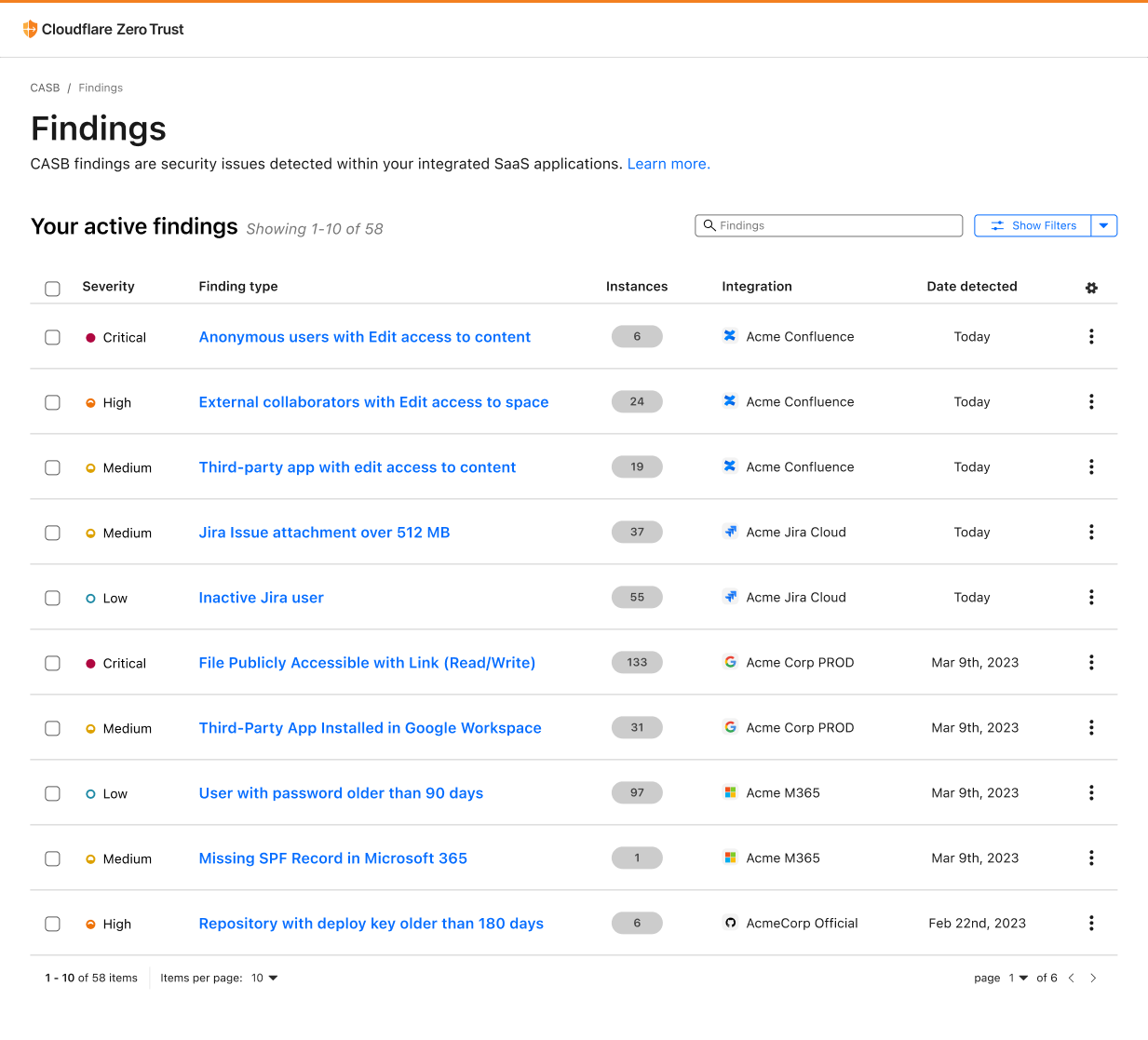
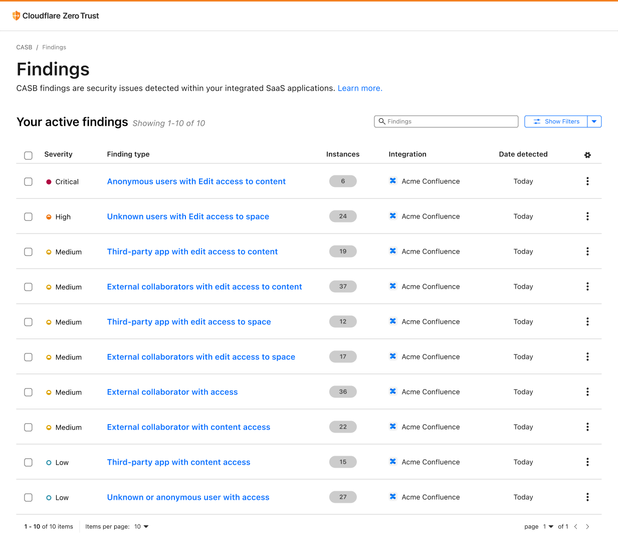
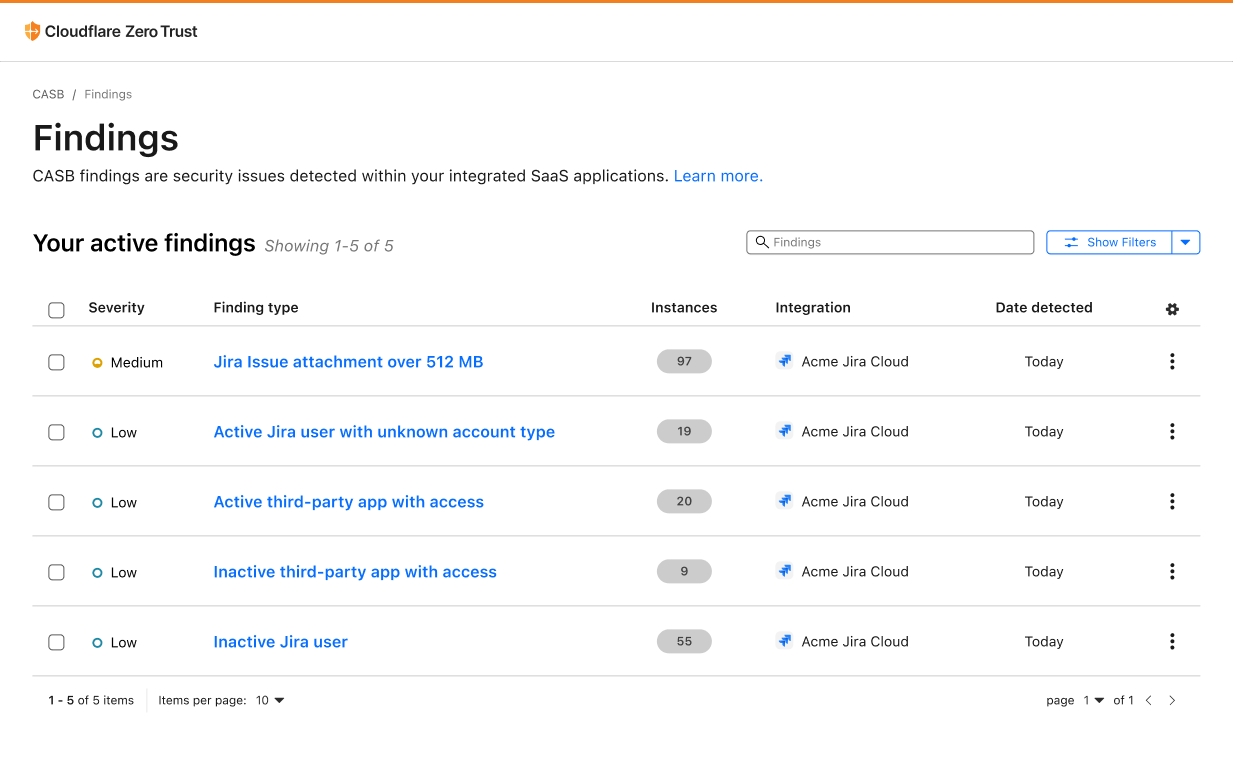


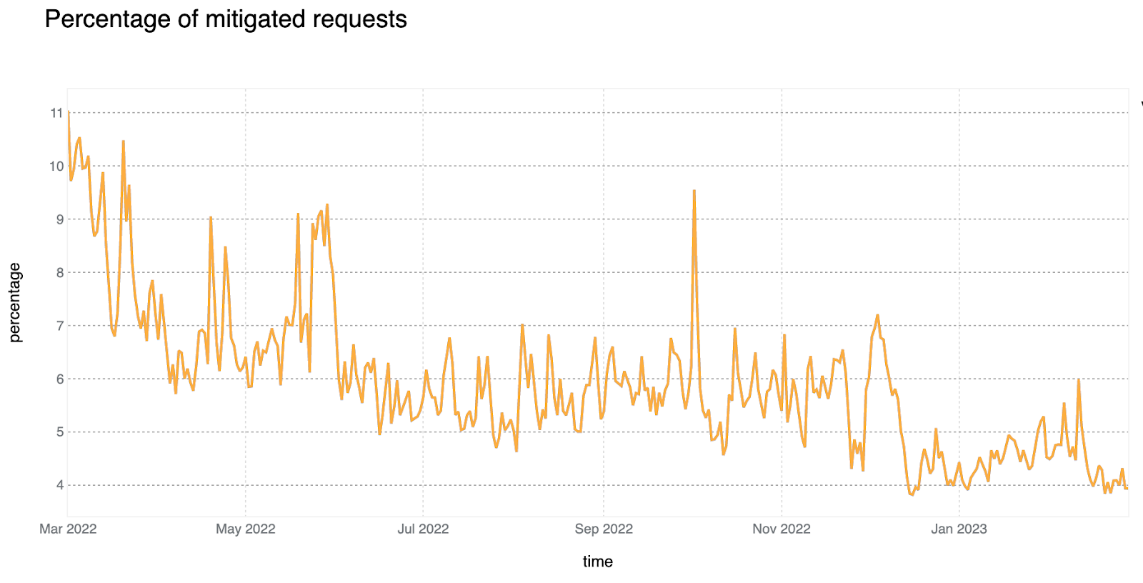
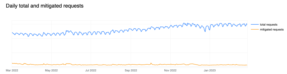

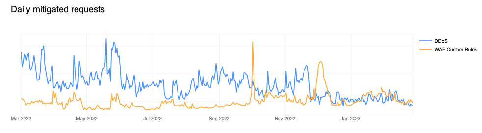
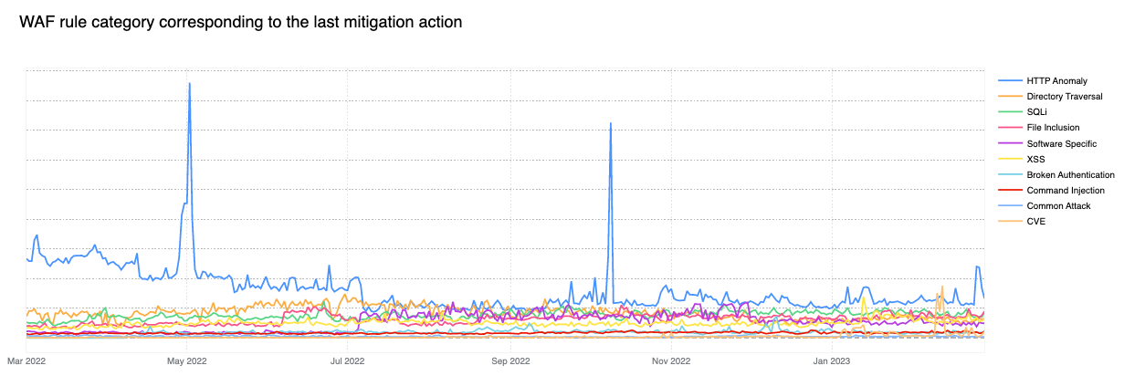
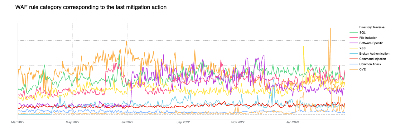
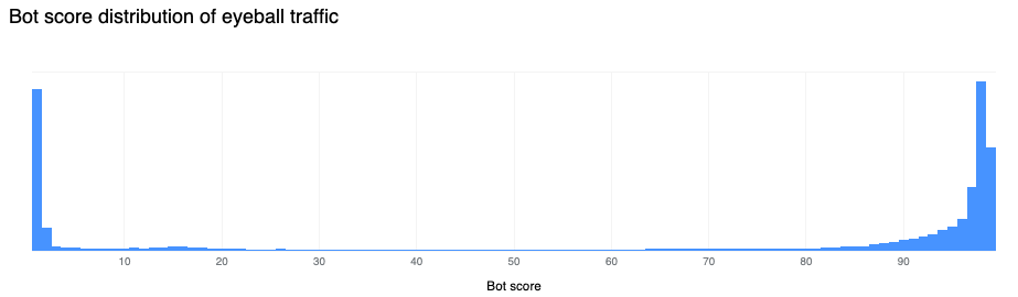
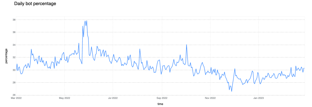
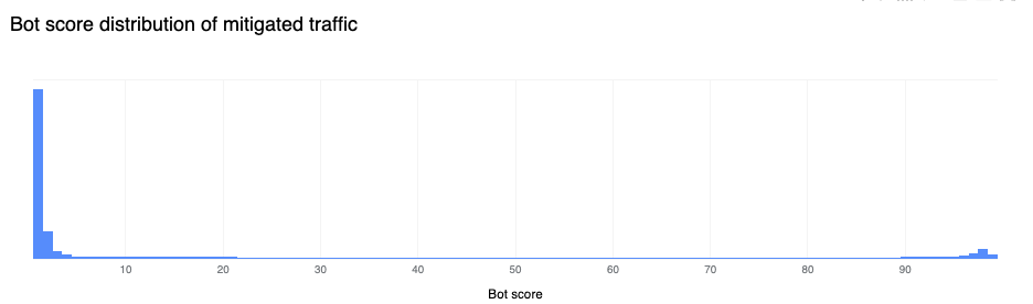

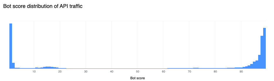

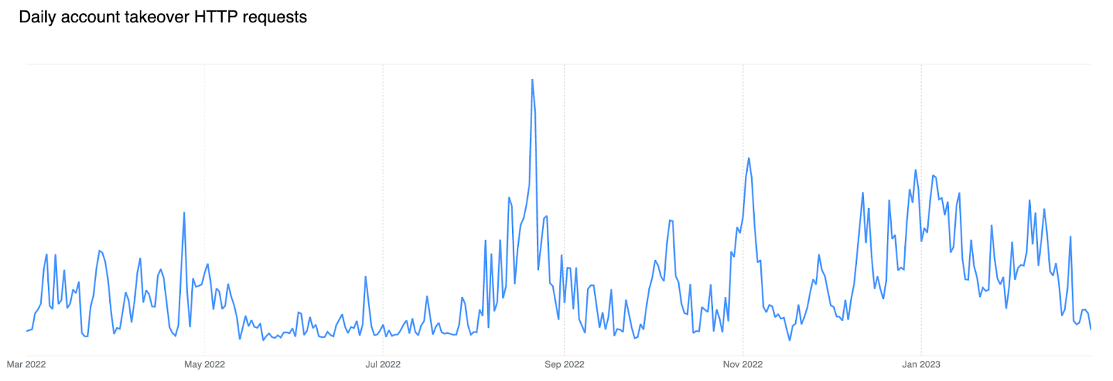


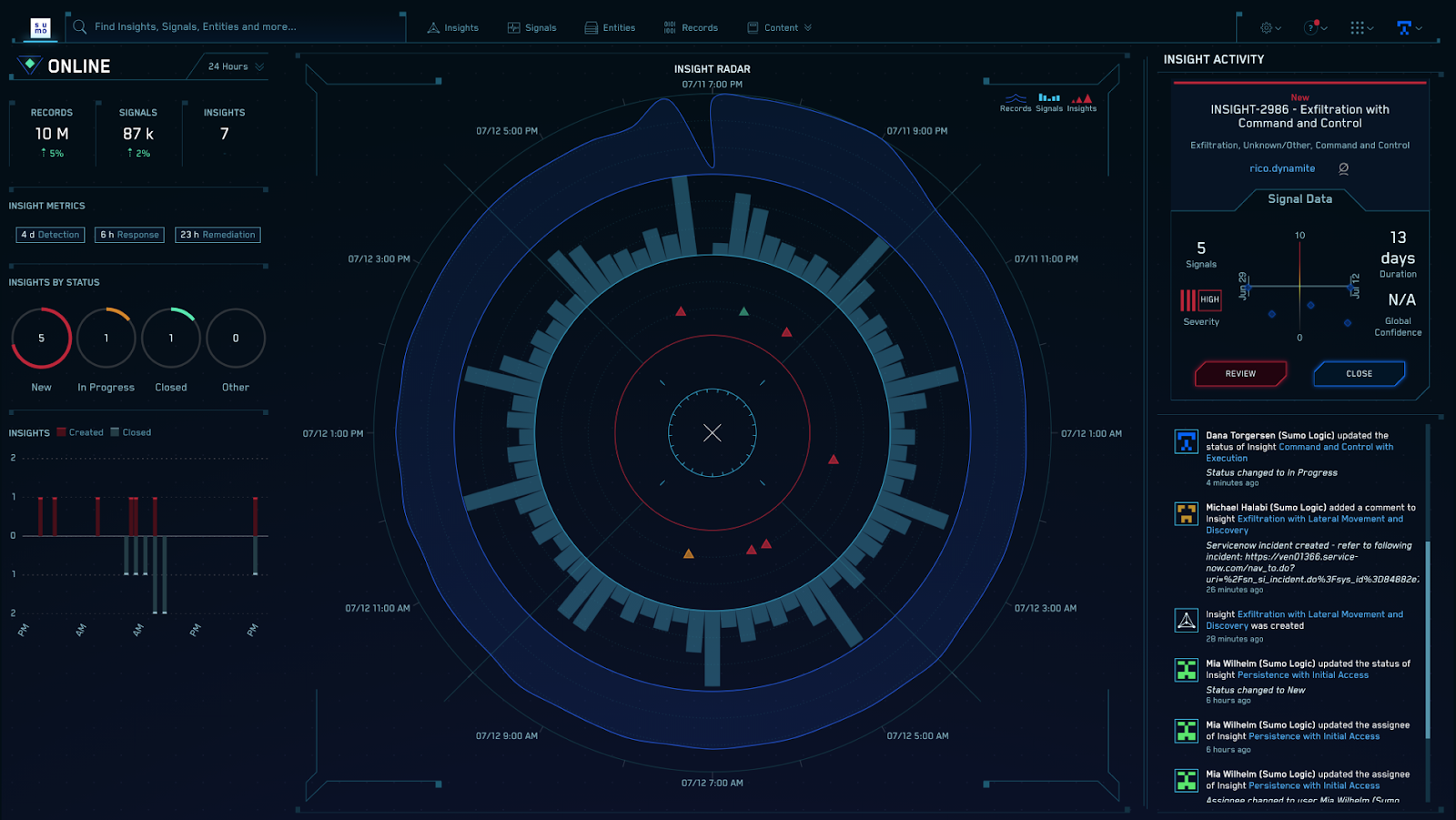


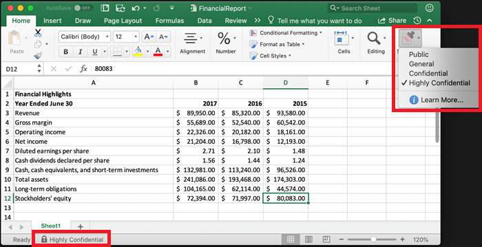
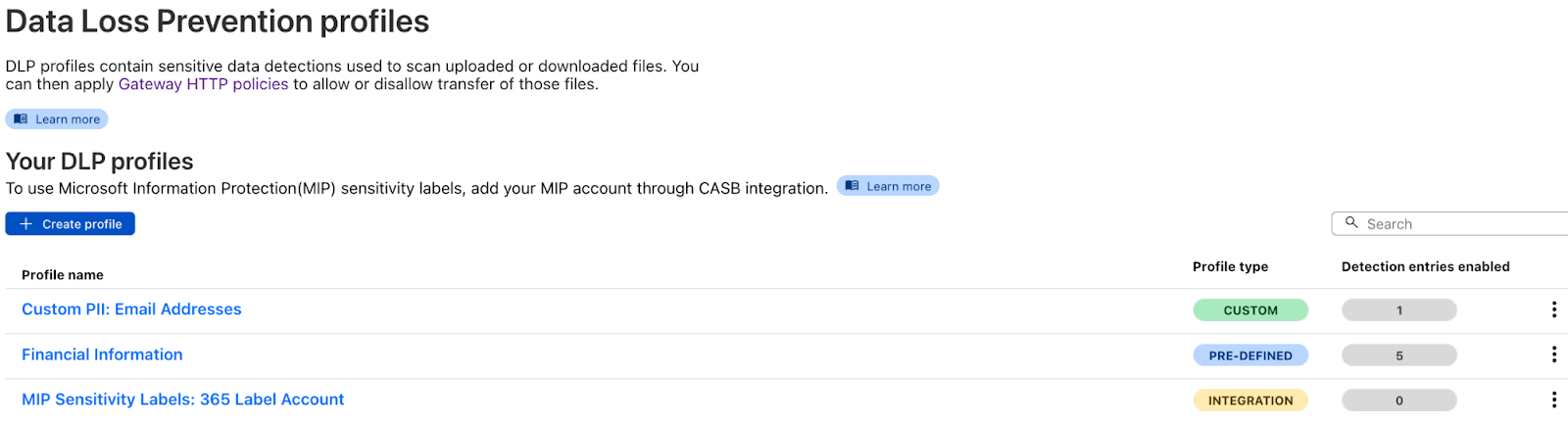
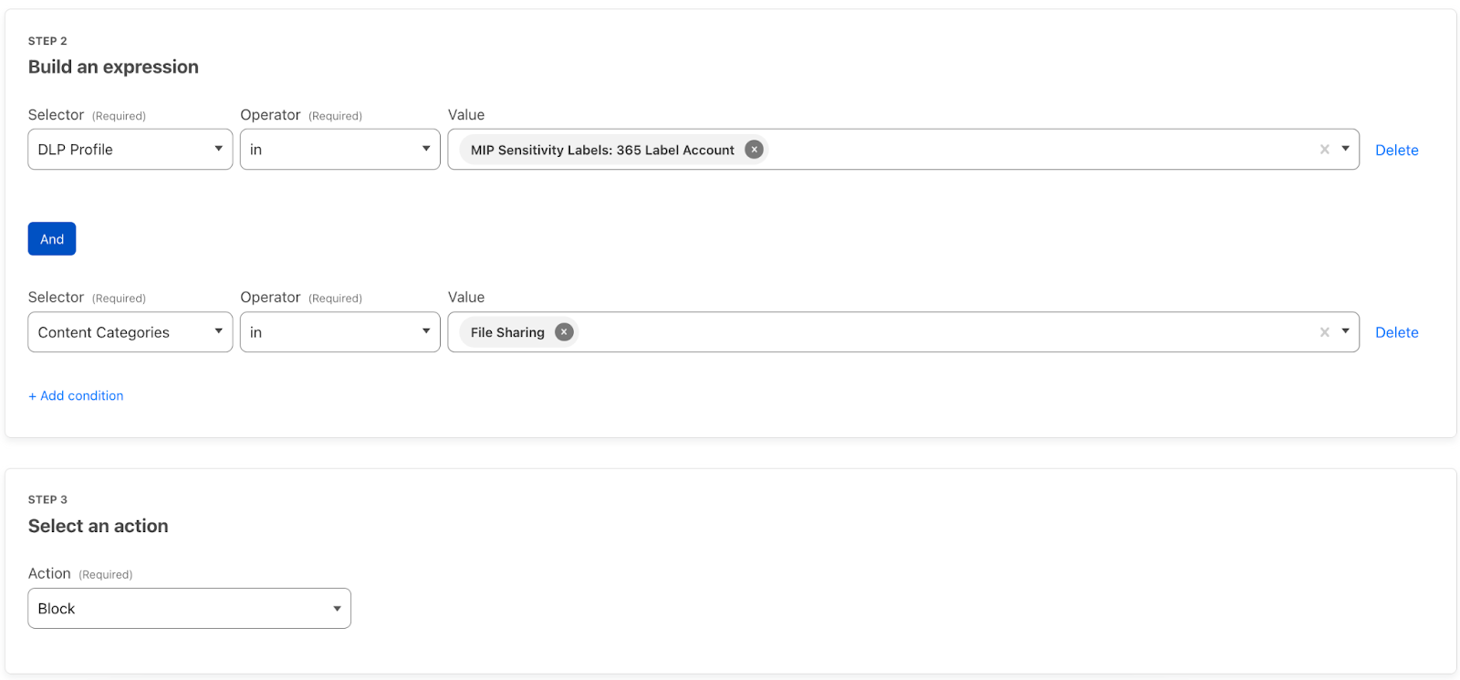


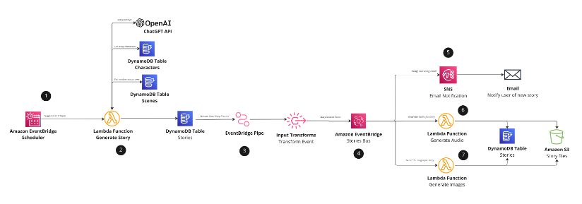

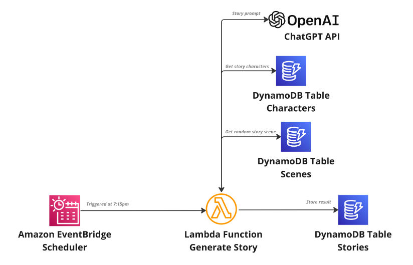


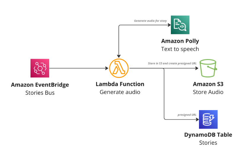


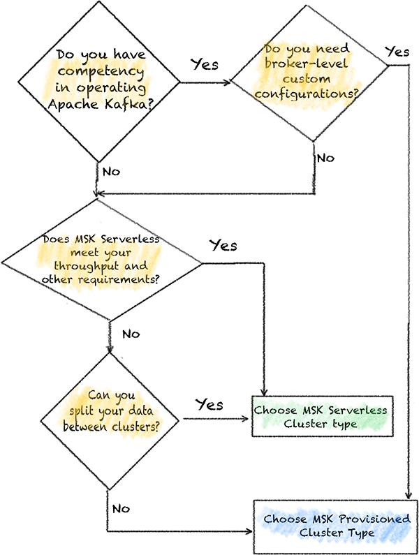
 Ali Alemi is a Streaming Specialist Solutions Architect at AWS. Ali advises AWS customers with architectural best practices and helps them design real-time analytics data systems that are reliable, secure, efficient, and cost-effective. He works backward from customers’ use cases and designs data solutions to solve their business problems. Prior to joining AWS, Ali supported several public sector customers and AWS consulting partners in their application modernization journey and migration to the cloud.