Post Syndicated from Faizan Ahmed original https://aws.amazon.com/blogs/big-data/provide-data-reliability-in-amazon-redshift-at-scale-using-great-expectations-library/
Ensuring data reliability is one of the key objectives of maintaining data integrity and is crucial for building data trust across an organization. Data reliability means that the data is complete and accurate. It’s the catalyst for delivering trusted data analytics and insights. Incomplete or inaccurate data leads business leaders and data analysts to make poor decisions, which can lead to negative downstream impacts and subsequently may result in teams spending valuable time and money correcting the data later on. Therefore, it’s always a best practice to run data reliability checks before loading the data into any targets like Amazon Redshift, Amazon DynamoDB, or Amazon Timestream databases.
This post discusses a solution for running data reliability checks before loading the data into a target table in Amazon Redshift using the open-source library Great Expectations. You can automate the process for data checks via the extensive built-in Great Expectations glossary of rules using PySpark, and it’s flexible for adding or creating new customized rules for your use case.
Amazon Redshift is a cloud data warehouse solution and delivers up to three times better price-performance than other cloud data warehouses. With Amazon Redshift, you can query and combine exabytes of structured and semi-structured data across your data warehouse, operational database, and data lake using standard SQL. Amazon Redshift lets you save the results of your queries back to your Amazon Simple Storage Service (Amazon S3) data lake using open formats like Apache Parquet, so that you can perform additional analytics from other analytics services like Amazon EMR, Amazon Athena, and Amazon SageMaker.
Great Expectations (GE) is an open-source library and is available in GitHub for public use. It helps data teams eliminate pipeline debt through data testing, documentation, and profiling. Great Expectations helps build trust, confidence, and integrity of data across data engineering and data science teams in your organization. GE offers a variety of expectations developers can configure. The tool defines expectations as statements describing verifiable properties of a dataset. Not only does it offer a glossary of more than 50 built-in expectations, it also allows data engineers and scientists to write custom expectation functions.
Use case overview
Before performing analytics or building machine learning (ML) models, cleaning data can take up a lot of time in the project cycle. Without automated and systematic data quality checks, we may spend most of our time cleaning data and hand-coding one-off quality checks. As most data engineers and scientists know, this process can be both tedious and error-prone.
Having an automated quality check system is critical to project efficiency and data integrity. Such systems help us understand data quality expectations and the business rules behind them, know what to expect in our data analysis, and make communicating the data’s intricacies much easier. For example, in a raw dataset of customer profiles of a business, if there’s a column for date of birth in format YYYY-mm-dd, values like 1000-09-01 would be correctly parsed as a date type. However, logically this value would be incorrect in 2021, because the age of the person would be 1021 years, which is impossible.
Another use case could be to use GE for streaming analytics, where you can use AWS Database Migration Service (AWS DMS) to migrate a relational database management system. AWS DMS can export change data capture (CDC) files in Parquet format to Amazon S3, where these files can then be cleansed by an AWS Glue job using GE and written to either a destination bucket for Athena consumption or the rows can be streamed in AVRO format to Amazon Kinesis or Kafka.
Additionally, automated data quality checks can be versioned and also bring benefit in the form of optimal data monitoring and reduced human intervention. Data lineage in an automated data quality system can also indicate at which stage in the data pipeline the errors were introduced, which can help inform improvements in upstream systems.
Solution architecture
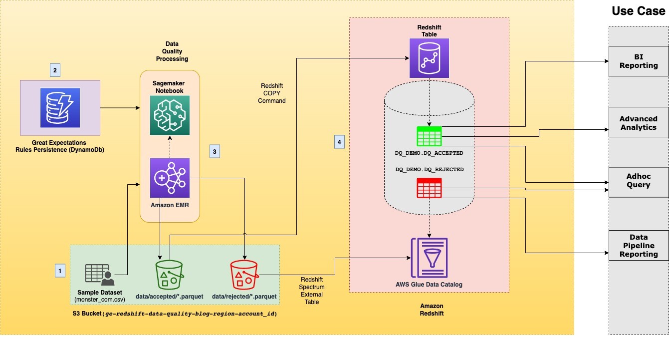
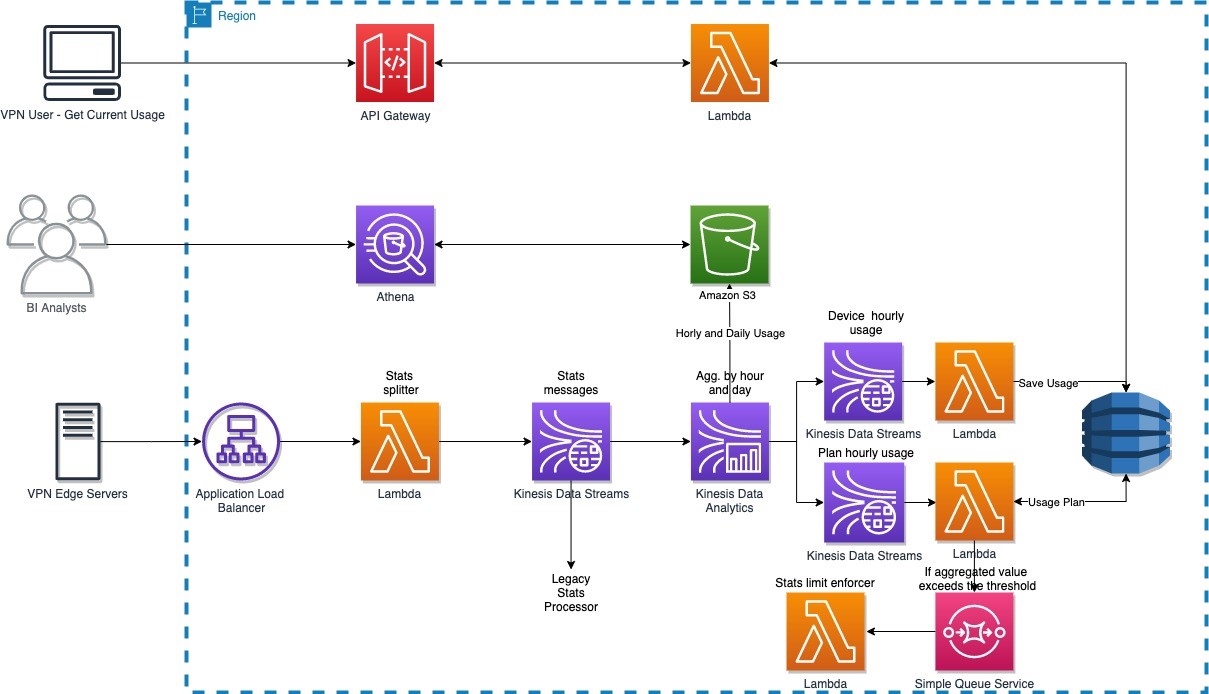
This post comes with a ready-to-use blueprint that automatically provisions the necessary infrastructure and spins up a SageMaker notebook that walks you step by step through the solution. Additionally, it enforces the best practices in data DevOps and infrastructure as code. The following diagram illustrates the solution architecture.

The architecture contains the following components:
- Data lake – When we run the AWS CloudFormation stack, an open-source sample dataset in CSV format is copied to an S3 bucket in your account. As an output of the solution, the data destination is an S3 bucket. This destination consists of two separate prefixes, each of which contains files in Parquet format, to distinguish between accepted and rejected data.
- DynamoDB – The CloudFormation stack persists data quality expectations in a DynamoDB table. Four predefined column expectations are populated by the stack in a table called
redshift-ge-dq-dynamo-blog-rules. Apart from the pre-populated rules, you can add any rule from the Great Expectations glossary according to the data model showcased later in the post.
- Data quality processing – The solution utilizes a SageMaker notebook instance powered by Amazon EMR to process the sample dataset using PySpark (v3.1.1) and Great Expectations (v0.13.4). The notebook is automatically populated with the S3 bucket location and Amazon Redshift cluster identifier via the SageMaker lifecycle config provisioned by AWS CloudFormation.
- Amazon Redshift – We create internal and external tables in Amazon Redshift for the accepted and rejected datasets produced from processing the sample dataset. The external
dq_rejected.monster_com_rejected table, for rejected data, uses Amazon Redshift Spectrum and creates an external database in the AWS Glue Data Catalog to reference the table. The dq_accepted.monster_com table is created as a regular Amazon Redshift table by using the COPY command.
Sample dataset
As part of this post, we have performed tests on the Monster.com job applicants sample dataset to demonstrate the data reliability checks using the Great Expectations library and loading data into an Amazon Redshift table.
The dataset contains nearly 22,000 different sample records with the following columns:
countrycountry_codedate_addedhas_expiredjob_boardjob_descriptionjob_titlejob_typelocationorganizationpage_urlsalarysectoruniq_id
For this post, we have selected four columns with inconsistent or dirty data, namely organization, job_type, uniq_id, and location, whose inconsistencies are flagged according to the rules we define from the GE glossary as described later in the post.
Prerequisites
For this solution, you should have the following prerequisites:
- An AWS account if you don’t have one already. For instructions, see Sign Up for AWS.
- For this post, you can launch the CloudFormation stack in the following Regions:
us-east-1us-east-2us-west-1us-west-2
- An AWS Identity and Access Management (IAM) user. For instructions, see Create an IAM User.
- The user should have create, write, and read access for the following AWS services:
- Familiarity with Great Expectations and PySpark.
Set up the environment
Choose Launch Stack to start creating the required AWS resources for the notebook walkthrough:

For more information about Amazon Redshift cluster node types, see Overview of Amazon Redshift clusters. For the type of workflow described in this post, we recommend using the RA3 Instance Type family.
Run the notebooks
When the CloudFormation stack is complete, complete the following steps to run the notebooks:
- On the SageMaker console, choose Notebook instances in the navigation pane.

This opens the notebook instances in your Region. You should see a notebook titled redshift-ge-dq-EMR-blog-notebook.
- Choose Open Jupyter next to this notebook to open the Jupyter notebook interface.
You should see the Jupyter notebook file titled ge-redshift.ipynb.
- Choose the file to open the notebook and follow the steps to run the solution.
Run configurations to create a PySpark context
When the notebook is open, make sure the kernel is set to Sparkmagic (PySpark). Run the following block to set up Spark configs for a Spark context.

Create a Great Expectations context
In Great Expectations, your data context manages your project configuration. We create a data context for our solution by passing our S3 bucket location. The S3 bucket’s name, created by the stack, should already be populated within the cell block. Run the following block to create a context:
from great_expectations.data_context.types.base import DataContextConfig,DatasourceConfig,S3StoreBackendDefaults
from great_expectations.data_context import BaseDataContext

bucket_prefix = "ge-redshift-data-quality-blog"
bucket_name = "ge-redshift-data-quality-blog-region-account_id"
region_name = '-'.join(bucket_name.replace(bucket_prefix,'').split('-')[1:4])
dataset_path=f"s3://{bucket_name}/monster_com-job_sample.csv"
project_config = DataContextConfig(
    config_version=2,
    plugins_directory=None,
    config_variables_file_path=None,
    datasources={
        "my_spark_datasource": {
            "data_asset_type": {
                "class_name": "SparkDFDataset",//Setting dataset type to Spark
                "module_name": "great_expectations.dataset",
            },
            "spark_config": dict(spark.sparkContext.getConf().getAll()) //Passing Spark Session configs,
            "class_name": "SparkDFDatasource",
            "module_name": "great_expectations.datasource"
        }
    },
    store_backend_defaults=S3StoreBackendDefaults(default_bucket_name=bucket_name)//
)
context = BaseDataContext(project_config=project_config)
For more details on creating a GE context, see Getting started with Great Expectations.
Get GE validation rules from DynamoDB
Our CloudFormation stack created a DynamoDB table with prepopulated rows of expectations. The data model in DynamoDB describes the properties related to each dataset and its columns and the number of expectations you want to configure for each column. The following code describes an example of the data model for the column organization:
{
 "id": "job_reqs-organization",
 "dataset_name": "job_reqs",
 "rules": [ //list of expectations to apply to this column
  {
   "kwargs": {
    "result_format": "SUMMARY|COMPLETE|BASIC|BOOLEAN_ONLY" //The level of detail of the result
   },
   "name": "expect_column_values_to_not_be_null",//name of GE expectation   "reject_msg": "REJECT:null_values_found_in_organization"
  }
 ],
 "column_name": "organization"
}
The code contains the following parameters:
- id – Unique ID of the document
- dataset_name – Name of the dataset, for example
monster_com
- rules – List of GE expectations to apply:
- kwargs – Parameters to pass to an individual expectation
- name – Name of the expectation from the GE glossary
- reject_msg – String to flag for any row that doesn’t pass this expectation
- column_name – Name of dataset column to run the expectations on
Each column can have one or more expectations associated that it needs to pass. You can also add expectations for more columns or to existing columns by following the data model shown earlier. With this technique, you can automate verification of any number of data quality rules for your datasets without performing any code change. Apart from its flexibility, what makes GE powerful is the ability to create custom expectations if the GE glossary doesn’t cover your use case. For more details on creating custom expectations, see How to create custom Expectations.
Now run the cell block to fetch the GE rules from the DynamoDB client:
- Read the
monster.com sample dataset and pass through validation rules.
After we have the expectations fetched from DynamoDB, we can read the raw CSV dataset. This dataset should already be copied to your S3 bucket location by the CloudFormation stack. You should see the following output after reading the CSV as a Spark DataFrame.
To evaluate whether a row passes each column’s expectations, we need to pass the necessary columns to a Spark user-defined function. This UDF evaluates each row in the DataFrame and appends the results of each expectation to a comments column.

Rows that pass all column expectations have a null value in the comments column.
A row that fails at least one column expectation is flagged with the string format REJECT:reject_msg_from_dynamo. For example, if a row has a null value in the organization column, then according to the rules defined in DynamoDB, the comments column is populated by the UDF as REJECT:null_values_found_in_organization.
The technique with which the UDF function recognizes a potentially erroneous column is done by evaluating the result dictionary generated by the Great Expectations library. The generation and structure of this dictionary is dependent upon the keyword argument of result_format. In short, if the count of unexpected column values of any column is greater than zero, we flag that as a rejected row.
- Split the resulting dataset into accepted and rejected DataFrames.
Now that we have all the rejected rows flagged in the source DataFrame within the comments column, we can use this property to split the original dataset into accepted and rejected DataFrames. In the previous step, we mentioned that we append an action message in the comments column for each failed expectation in a row. With this fact, we can select rejected rows that start with the string REJECT (alternatively, you can also filter by non-null values in the comments column to get the accepted rows). When we have the set of rejected rows, we can get the accepted rows as a separate DataFrame by using the following PySpark except function.

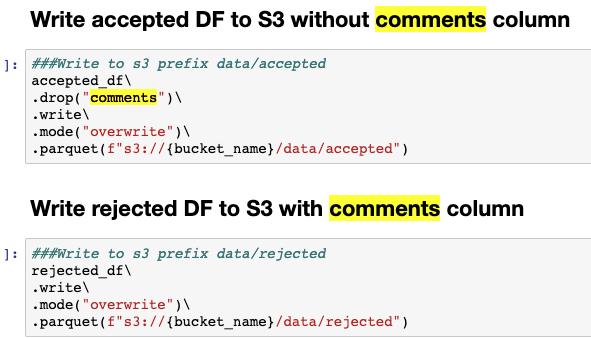
Write the DataFrames to Amazon S3.
Now that we have the original DataFrame divided, we can write them both to Amazon S3 in Parquet format. We need to write the accepted DataFrame without the comments column because it’s only added to flag rejected rows. Run the cell blocks to write the Parquet files under appropriate prefixes as shown in the following screenshot.

Copy the accepted dataset to an Amazon Redshift table
Now that we have written the accepted dataset, we can use the Amazon Redshift COPY command to load this dataset into an Amazon Redshift table. The notebook outlines the steps required to create a table for the accepted dataset in Amazon Redshift using the Amazon Redshift Data API. After the table is created successfully, we can run the COPY command.
Another noteworthy point to mention is that one of the advantages that we witness due to the data quality approach described in this post is that the Amazon Redshift COPY command doesn’t fail due to schema or datatype errors for the columns, which have clear expectations defined that match the schema. Similarly, you can define expectations for every column in the table that satisfies the schema constraints and can be considered a dq_accepted.monster_com row.
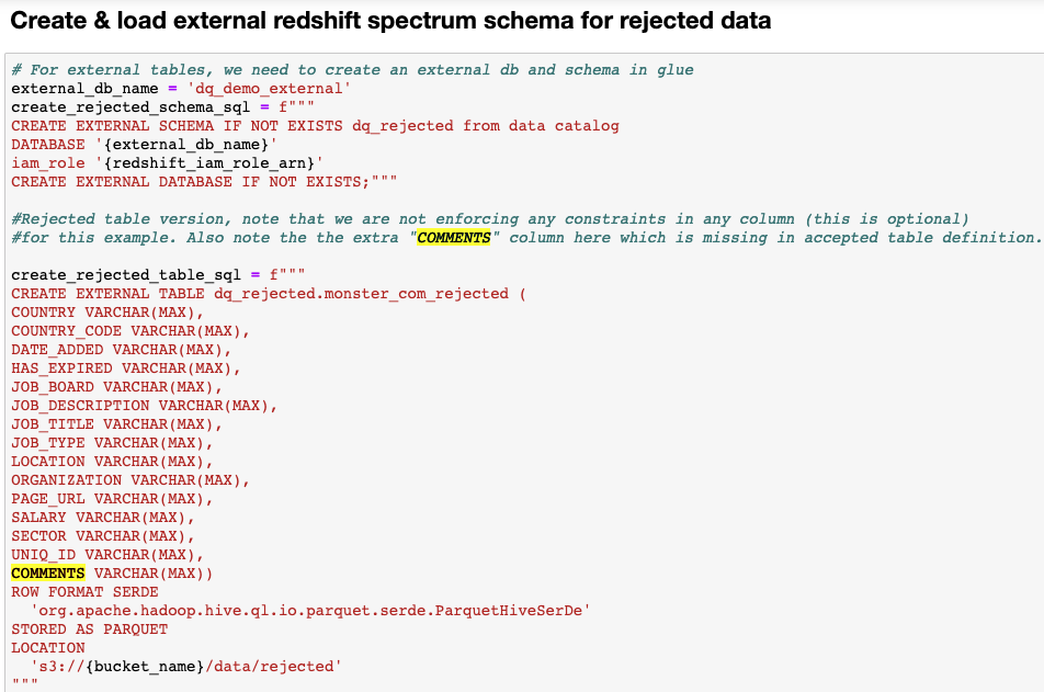
Create an external table in Amazon Redshift for rejected data
We need to have the rejected rows available to us in Amazon Redshift for comparative analysis. These comparative analyses can help inform upstream systems regarding the quality of data being collected and how they can be corrected to improve the overall quality of data. However, it isn’t wise to store the rejected data on the Amazon Redshift cluster, particularly for large tables, because it occupies extra disk space and increase cost. Instead, we use Redshift Spectrum to register an external table in an external schema in Amazon Redshift. The external schema lives in an external database in the AWS Glue Data Catalog and is referenced by Amazon Redshift. The following screenshot outlines the steps to create an external table.

Verify and compare the datasets in Amazon Redshift.
12,160 records got processed successfully out of a total of 22,000 from the input dataset, and were loaded to the monster_com table under the dq_accepted schema. These records successfully passed all the validation rules configured in DynamoDB.

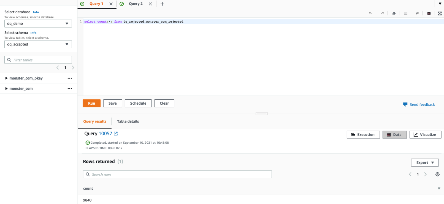
A total 9,840 records got rejected due to breaking of one or more rules configured in DynamoDB and loaded to the monster_com_rejected table in the dq_rejected schema. In this section, we describe the behavior of each expectation on the dataset.

- Expect column values to not be null in
organization – This rule is configured to reject a row if the organization is null. The following query returns the sample of rows, from the dq_rejected.monster_com_rejected table, that are null in the organization column, with their reject message.

- Expect column values to match the regex list in
job_type – This rule expects the column entries to be strings that can be matched to either any of or all of a list of regular expressions. In our use case, we have only allowed values that match a pattern within [".*Full.*Time", ".*Part.*Time", ".*Contract.*"].
- The following query shows rows that are rejected due to an invalid job type.

Most of the records were rejected with multiple reasons, and all those mismatches are captured under the comments column.
- Expect column values to not match regex for
uniq_id – Similar to the previous rule, this rule aims to reject any row whose value matches a certain pattern. In our case, that pattern is having an empty space (\s++) in the primary column uniq_id. This means we consider a value to be invalid if it has empty spaces in the string. The following query returned an invalid format for uniq_id.

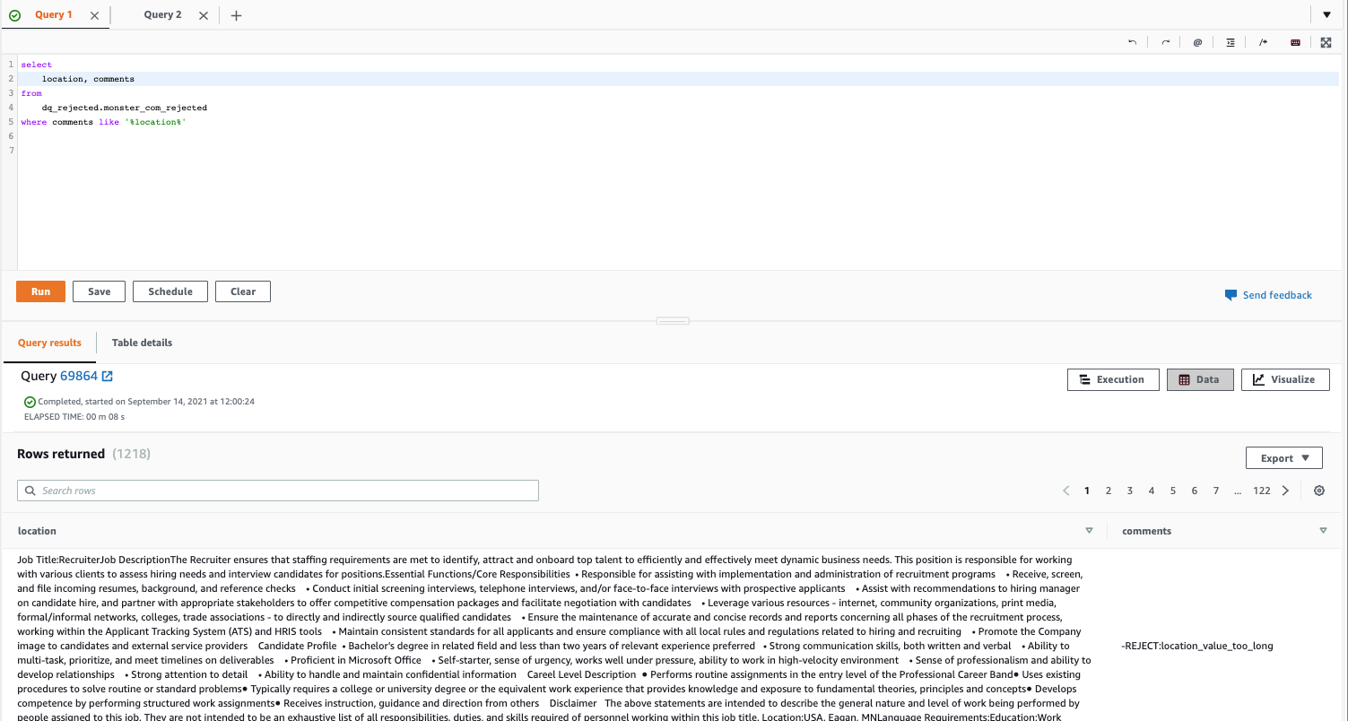
- Expect column entries to be strings with a length between a minimum value and a maximum value (inclusive) – A length check rule is defined in the DynamoDB table for the
location column. This rule rejects values or rows if the length of the value violates the specified constraints. The following
- query returns the records that are rejected due to a rule violation in the
location column.

You can continue to analyze the other columns’ predefined rules from DynamoDB or pick any rule from the GE glossary and add it to an existing column. Rerun the notebook to see the result of your data quality rules in Amazon Redshift. As mentioned earlier, you can also try creating custom expectations for other columns.
Benefits and limitations
The efficiency and efficacy of this approach is delineated from the fact that GE enables automation and configurability to an extensive degree when compared with other approaches. A very brute force alternative to this could be writing stored procedures in Amazon Redshift that can perform data quality checks on staging tables before data is loaded into main tables. However, this approach might not be scalable because you can’t persist repeatable rules for different columns, as persisted here in DynamoDB, in stored procedures (or call DynamoDB APIs), and would have to write and store a rule for each column of every table. Furthermore, to accept or reject a row based on a single rule requires complex SQL statements that may result in longer durations for data quality checks or even more compute power, which can also incur extra costs. With GE, a data quality rule is generic, repeatable, and scalable across different datasets.
Another benefit of this approach, related to using GE, is that it supports multiple Python-based backends, including Spark, Pandas, and Dask. This provides flexibility across an organization where teams might have skills in different frameworks. If a data scientist prefers using Pandas to write their ML pipeline feature quality test, then a data engineer using PySpark can use the same code base to extend those tests due to the consistency of GE across backends.
Furthermore, GE is written natively in Python, which means it’s a good option for engineers and scientists who are more used to running their extract, transform, and load (ETL) workloads in PySpark in comparison to frameworks like Deequ, which is natively written in Scala over Apache Spark and fits better for Scala use cases (the Python interface, PyDeequ, is also available). Another benefit of using GE is the ability to run multi-column unit tests on data, whereas Deequ doesn’t support that (as of this writing).
However, the approach described in this post might not be the most performant in some cases for full table load batch reads for very large tables. This is due to the serde (serialization/deserialization) cost of using UDFs. Because the GE functions are embedded in PySpark UDFs, the performance of these functions is slower than native Spark functions. Therefore, this approach gives the best performance when integrated with incremental data processing workflows, for example using AWS DMS to write CDC files from a source database to Amazon S3.
Clean up
Some of the resources deployed in this post, including those deployed using the provided CloudFormation template, incur costs as long as they’re in use. Be sure to remove the resources and clean up your work when you’re finished in order to avoid unnecessary cost.
Go to the CloudFormation console and click the ‘delete stack’ to remove all resources.
The resources in the CloudFormation template are not production ready. If you would like to use this solution in production, enable logging for all S3 buckets and ensure the solution adheres to your organization’s encryption policies through EMR Security Best Practices.
Conclusion
In this post, we demonstrated how you can automate data reliability checks using the Great Expectations library before loading data into an Amazon Redshift table. We also showed how you can use Redshift Spectrum to create external tables. If dirty data were to make its way into the accepted table, all downstream consumers such as business intelligence reporting, advanced analytics, and ML pipelines can get affected and produce inaccurate reports and results. The trends of such data can generate wrong leads for business leaders while making business decisions. Furthermore, flagging dirty data as rejected before loading into Amazon Redshift also helps reduce the time and effort a data engineer might have to spend in order to investigate and correct the data.
We are interested to hear how you would like to apply this solution for your use case. Please share your thoughts and questions in the comments section.
About the Authors
 Faizan Ahmed is a Data Architect at AWS Professional Services. He loves to build data lakes and self-service analytics platforms for his customers. He also enjoys learning new technologies and solving, automating, and simplifying customer problems with easy-to-use cloud data solutions on AWS. In his free time, Faizan enjoys traveling, sports, and reading.
 Bharath Kumar Boggarapu is a Data Architect at AWS Professional Services with expertise in big data technologies. He is passionate about helping customers build performant and robust data-driven solutions and realize their data and analytics potential. His areas of interests are open-source frameworks, automation, and data architecting. In his free time, he loves to spend time with family, play tennis, and travel.