Post Syndicated from Sébastien Stormacq original https://aws.amazon.com/blogs/aws/amazon-route-53-application-recovery-controller/
I am pleased to announce the availability today of Amazon Route 53 Application Recovery Controller, a Amazon Route 53 set of capabilities that continuously monitors an application’s ability to recover from failures and controls application recovery across multiple AWS Availability Zones, AWS Regions, and on premises environments to help you to build applications that must deliver very high availability.
At AWS, the security and availability of your data and workloads are our top priorities. From the very beginning, AWS global infrastructure allowed you to build application architectures that are resilient to different type of failures. When your business or application requires high availability, you typically use AWS global infrastructure to deploy redundant application replicas across AWS Availability Zones inside an AWS Region. Then, you use a Network or Application Load Balancer to route traffic to the appropriate replica. This architecture handles the requirements of the vast majority of workloads.
However, some industries and workloads have higher requirements in terms of high availability: availability rate at or above 99.99% with recovery time objectives (RTO) measured in seconds or minutes. Think about how real-time payment processing or trading engines can affect entire economies if disrupted. To address these requirements, you typically deploy multiple replicas across a variety of AWS Availability Zones, AWS Regions, and on premises environments. Then, you use Amazon Route 53 to reliably route end users to the appropriate replica.
Amazon Route 53 Application Recovery Controller helps you to build these applications requiring very high availability and low RTO, typically those using active-active architectures, but other type of redundant architectures might also benefit from Amazon Route 53 Application Recovery Controller. It is made of two parts: readiness check and routing control.
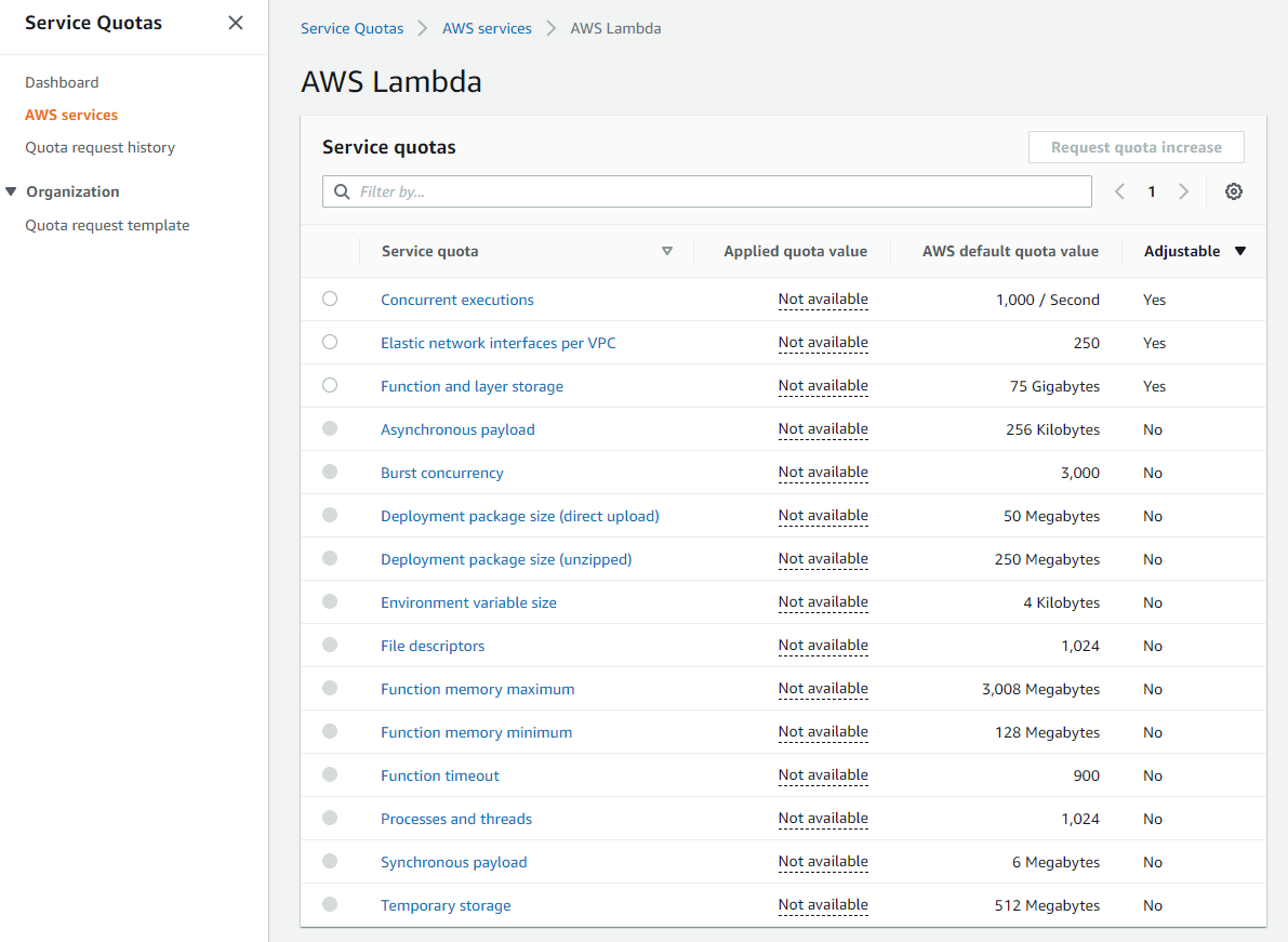
Readiness checks continuously monitor AWS resource configurations, capacity, and network routing policies, and allow you to monitor for any changes that would affect the ability to execute a recovery operation. These checks ensure that the recovery environment is scaled and configured to take over when needed. They check the configuration of Auto Scaling groups, Amazon Elastic Compute Cloud (Amazon EC2) instances, Amazon Elastic Block Store (EBS) volumes, load balancers, Amazon Relational Database Service (RDS) instances, Amazon DynamoDB tables, and several others. For example, readiness check verifies AWS service limits to ensure enough capacity can be deployed in an AWS Region in case of failover. It also verifies capacity and scaling characteristics of application replicas are the same across AWS Region.
Routing controls help to rebalance traffic across application replicas during failures, to ensure that the application stays available. Routing controls work with Amazon Route 53 health checks to redirect traffic to an application replica, using DNS resolution. Routing controls improve traditional automated Amazon Route 53 health check-based failovers in three ways:
- First, routing controls give you a way to failover the entire application stack based on application metrics or partial failures, such as a 5% increased error rate or a millisecond of increased latency.
- Second, routing controls give you safe and simple manual overrides. You can use them to shift traffic for maintenance purposes or to recover from failures when your monitors fail to detect an issue.
- Third, routing controls can use a capability called safety rules to prevent common side effects associated with fully automated health checks, such as preventing fail over to an unprepared replica, or flapping issues.
To help you understand how Route 53 Application Recovery Controller works, I’ll walk you through the process I used to configure my own high availability application.
How It Works
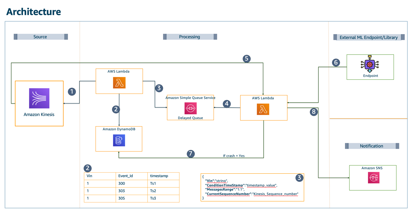
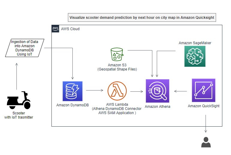
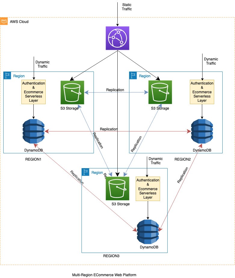
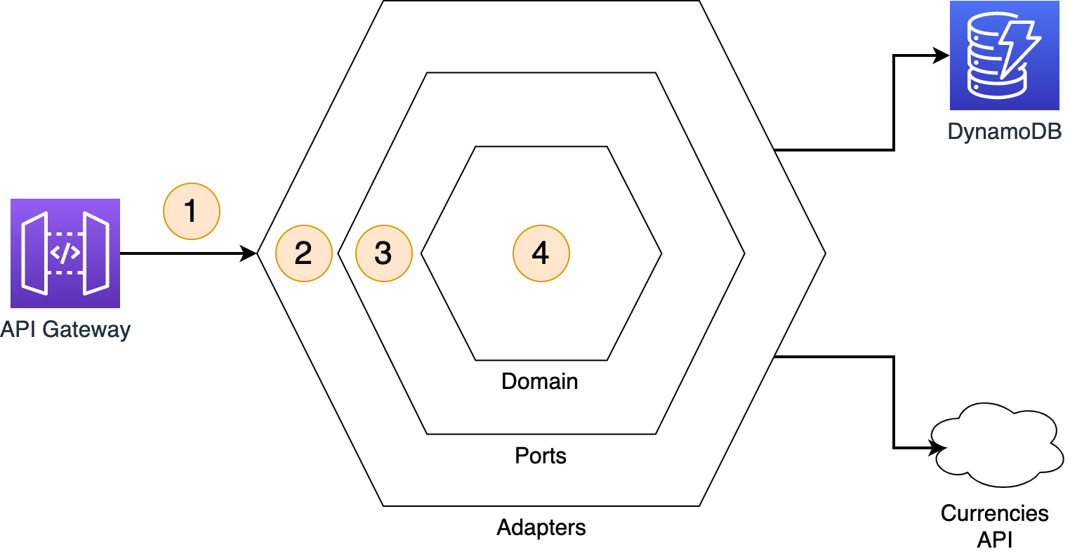
For demo purposes, I built an application made up of a load balancer, an Auto Scaling group with two EC2 instances, and a global DynamoDB table. I wrote a CDK script to deploy the application in two AWS Regions: US East (N. Virginia) and US West (Oregon). The global DynamoDB table ensures data is replicated across the two AWS Regions. This is an active-standby architecture, as I described earlier.
The application is a multi-player TicTacToe game, an application that typically needs 99.99% availability or more :-). One DNS record (tictactoe.seb.go-aws.com) points to the load balancer in the US East (N. Virginia) region. The following diagram shows the architecture for this application:

Preparing My Application
To configure Route 53 Application Recovery Controller for my application, I first deployed independent replicas of my application stack so that I can fail over traffic across the stacks. These copies are deployed across AWS high-availability boundaries, such as Availability Zones, or AWS Regions. I chose to deploy my application replicas across multiple AWS Regions
Then, I configured data replication across these independent replicas. I’m using DynamoDB global tables to help replicate my data.
Lastly, I configured each independent stack to expose a DNS name. This DNS name is the entry point into my application, such as a regional load balancer DNS name.
Terminology
Before I configure readiness check, let me share some basic terminology.
A cell defines the silo that contains my application’s independent units of failover. It groups all AWS resources that are required for my application to operate independently. For my demo, I have two cells: one per AWS Region where my application is deployed. A cell is typically aligned with AWS high-availability boundaries, such as AWS Regions or Availability Zones, but it can be smaller too. It is possible to have multiple cells in one Availability Zone. This is an effective way to reduce blast radius, especially when you follow one-cell-at-a-time change management practices.

A recovery group is a collection of cells that represent an application or group of applications that I want to check for failover readiness. A recovery group typically consists of two or more cells that mirror each other in terms of functionality.

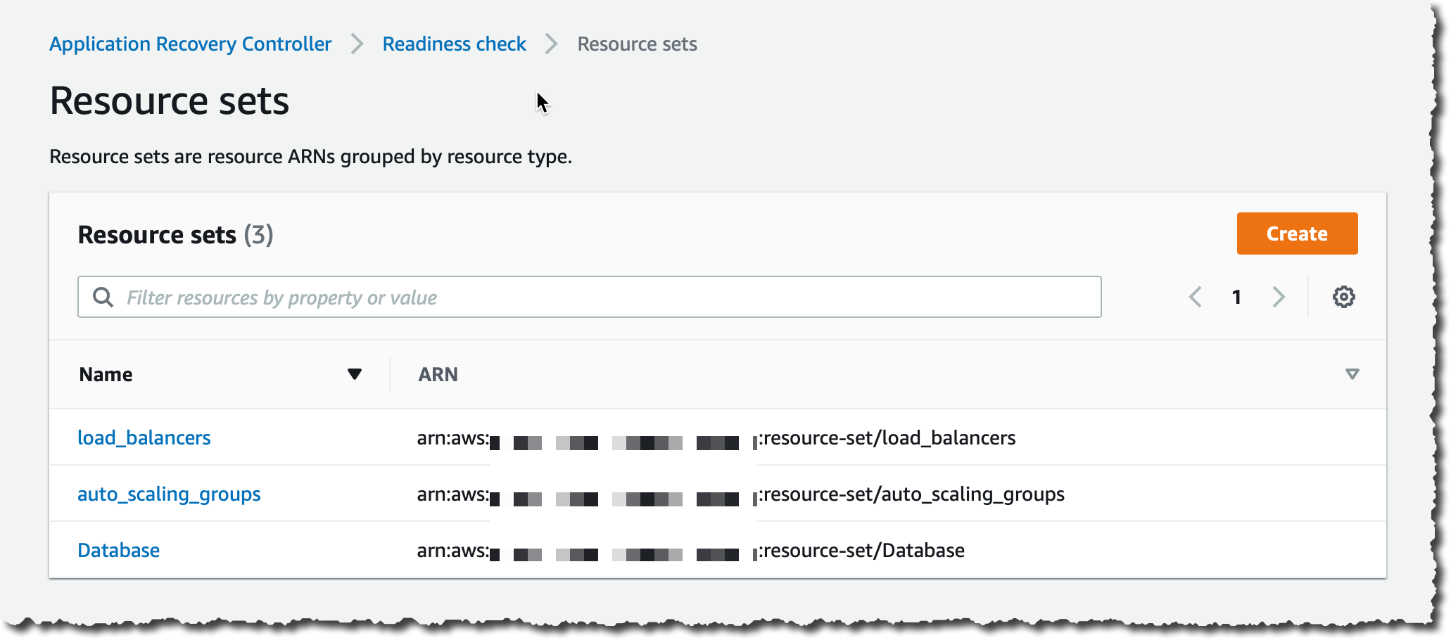
A resource set is a set of AWS resources that can span multiple cells. For this demo, I have three resource sets: one for the two load balancers in us-east-1 and us-west-2, one for the two Auto Scaling groups in the two Regions, and one for the global DynamoDB table.
A readiness check validates a set of AWS resources readiness to be failed over to. In this example, I want to audit readiness for my load balancers, Auto Scaling groups, and DynamoDB table. I create a readiness check for the Auto Scaling groups. The service constantly monitors the instance types and counts in the groups to make sure that each group is scaled equally. I repeat the process for the load balancer and the global DynamoDB table.

To help determine recovery readiness for my application, Route 53 Application Recovery Controller continuously audits mismatches in capacity, AWS resource limits, and AWS throttle limits across application cells (Availability Zones or Regions). When Route 53 Application Recovery Controller detects a mismatch in limits, it raises an AWS Service Quota request for the resource across the cells. If Route 53 Application Recovery Controller detects a capacity mismatch in resources, I can take actions to align capacity across the cells. For example, I could trigger a scaling increase for my Auto Scaling groups.
Create a Readiness Check
To create a readiness check, I open the AWS Management Console and navigate to the Application Recovery Controller section under Route 53.

To create a recovery group for my application, I navigate to the Getting Started section, then I choose Create recovery group.

I enter a name (for example AWSNewsBlogDemo) and then choose Next.

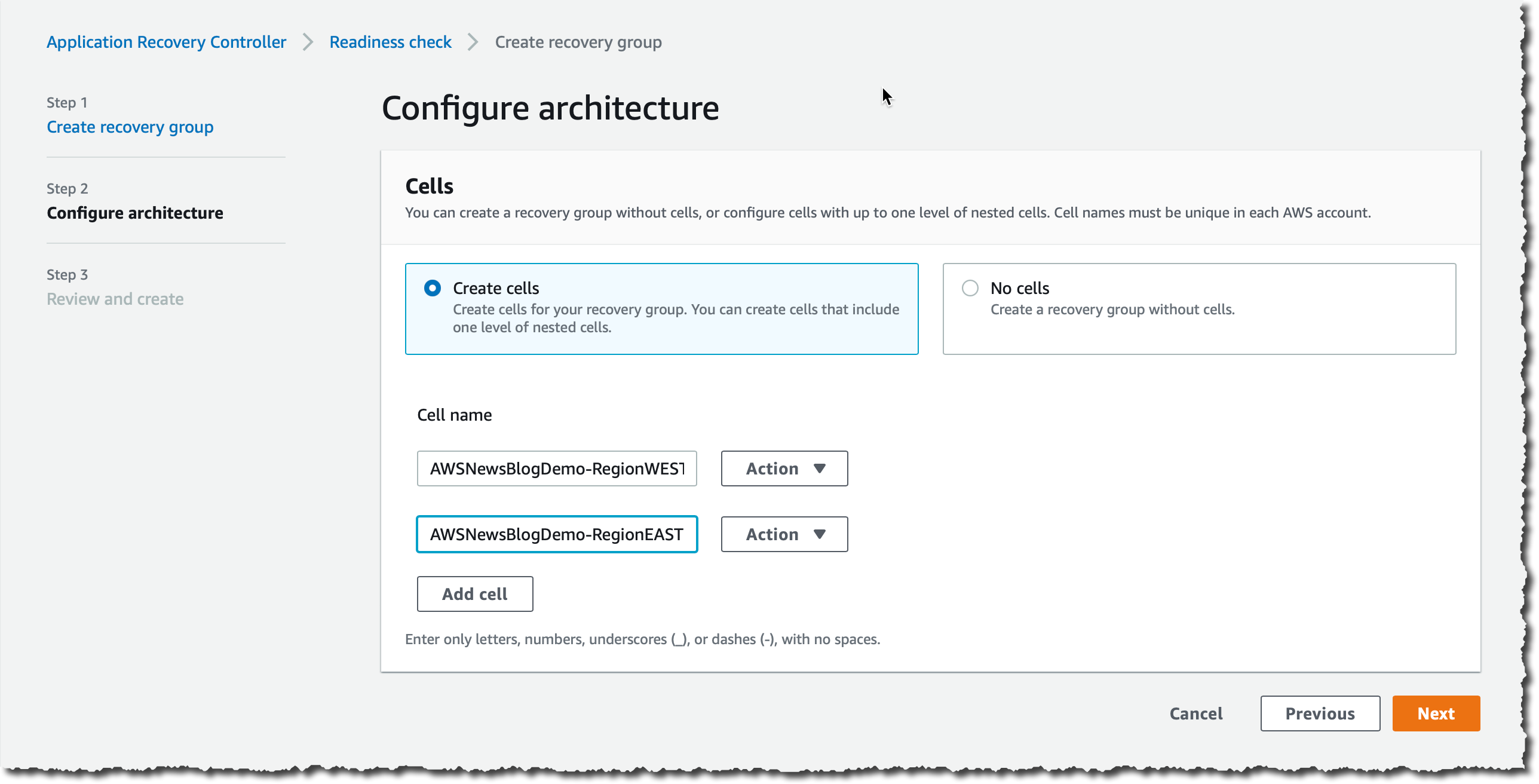
In Configure Architecture, I choose Add Cell, then I enter a cell name (AWSNewsBlogDemo-RegionWEST) and then choose Add Cell again to add a second cell. I enter AWSNewsBlogDemo-RegionEAST for the second cell. I choose Next to review my inputs, then I choose Create recovery group.
I now need to associate resources such as my load balancers, Auto Scaling groups, and DynamoDB table with my recovery group.

In the left navigation pane, I choose Resource Set and then I choose Create.

I enter a name for my first resource set (for example, load_balancers). For Resource type, I choose Network Load Balancer or Application Load Balancer and I then choose Add to add the load balancer ARN.
I choose Add again to enter the second load balancer ARN, and then I choose Create resource set.
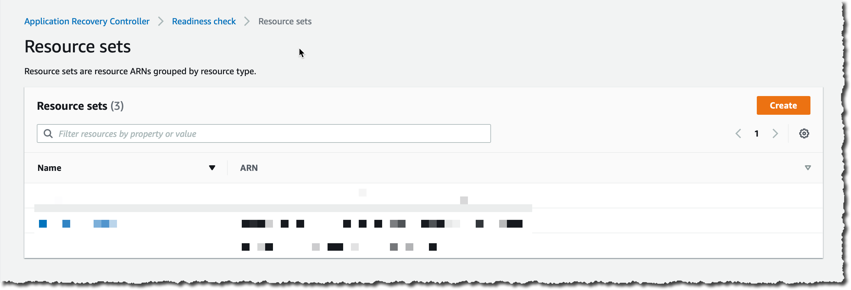
I repeat the process to create one resource set for the two Auto Scaling groups and a third resource set for the global DynamoDB table (one ARN). I now have three resource sets:

My last step is to create the readiness check. This will associate the resources with cells in the resource groups.

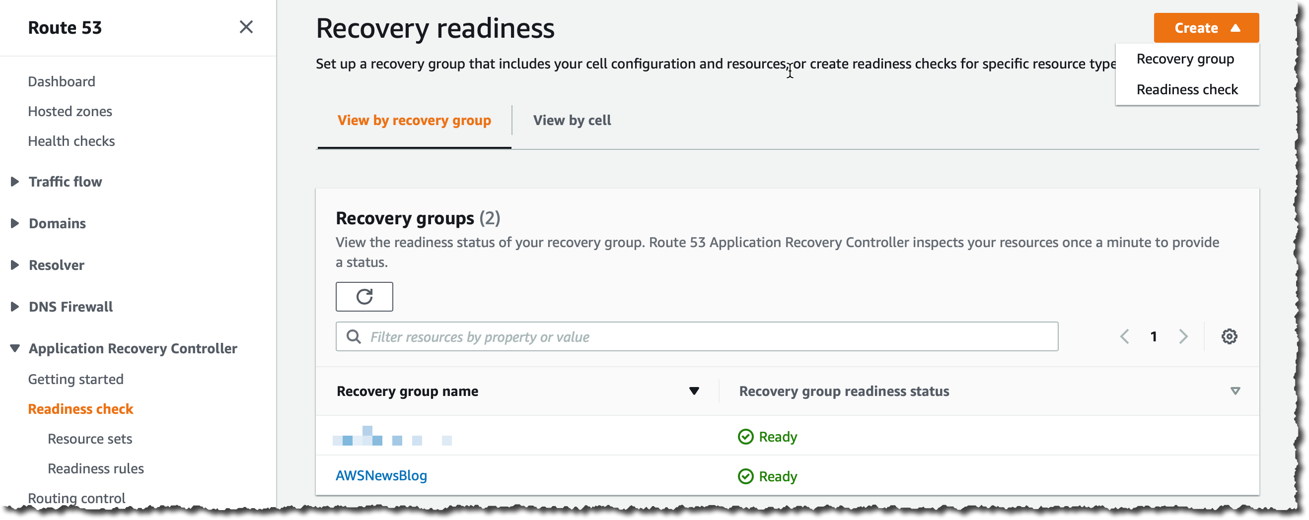
In Readiness check, I choose Create at the top right of the screen, then Readiness check.

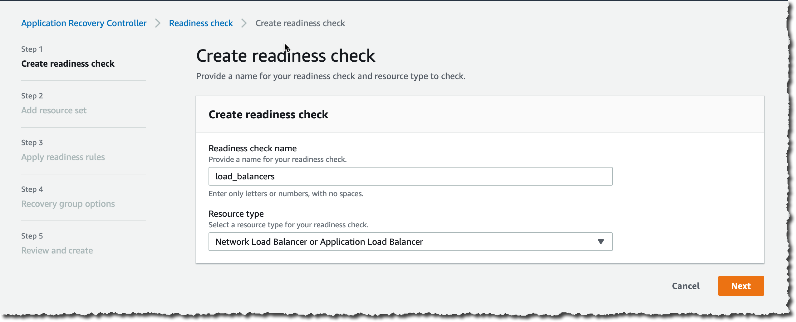
Step 1 (Create readiness check), I enter a name (for example, load_balancers). For Resource Type, I choose Network Load Balancer or Application Load Balancer and then choose Next.

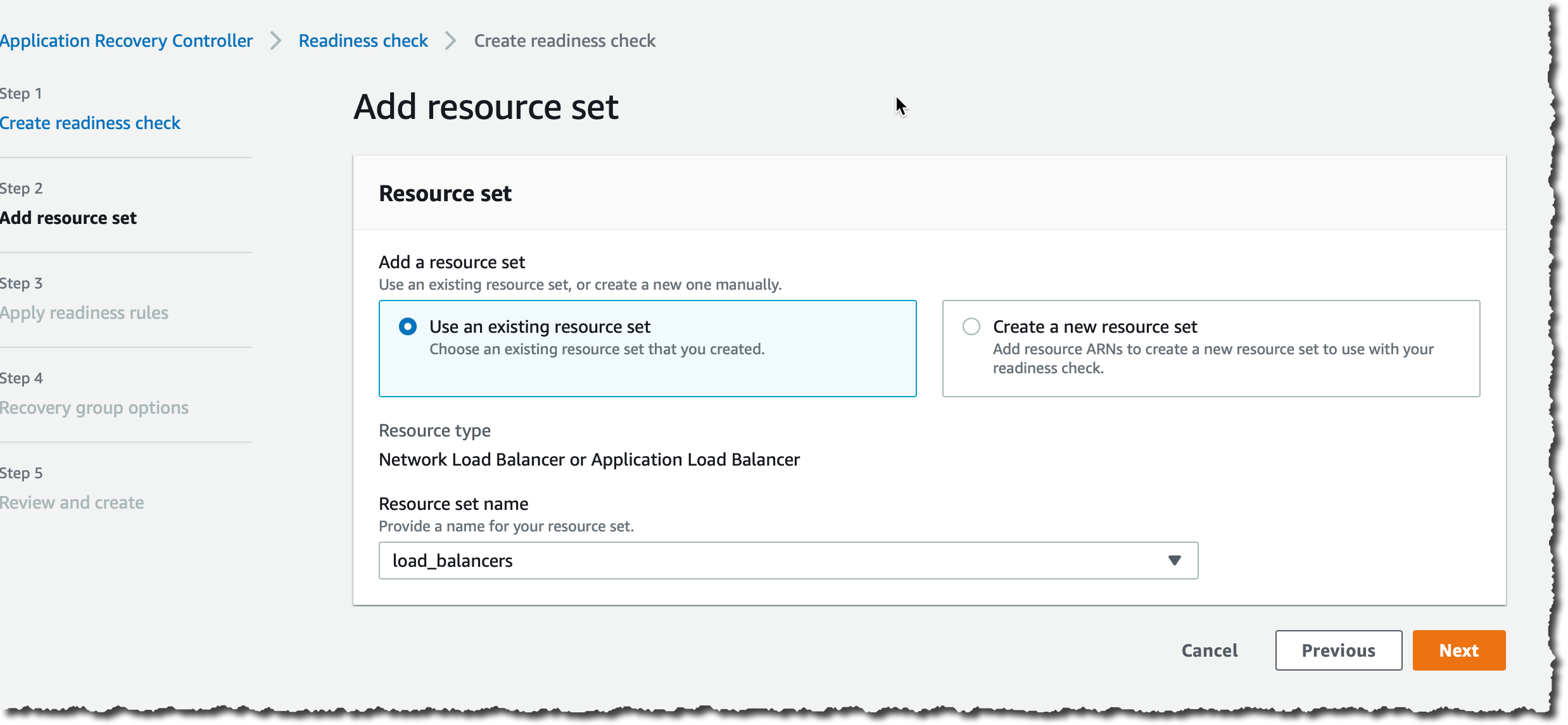
Step 2 (Add resource set), I keep the default selection Use an existing resource set and for Resource set name, I choose load_balancers and then I choose Next.
Step 3 (Apply readiness rules), I review the rules and then choose Next.

Step 4 (Recovery Group Options), I keep the default selection Associate with an existing recovery group. For Recovery group name, I choose AWSNewsBlog. Then, I associate the two cells (EAST and WEST) with the two load balancers ARN. Be sure to associate the correct load balancer to each cell. The Region name is included in the ARN.
Step 5 (Review and create), I review my choices and then choose Create readiness check.

I repeat this process for the Auto Scaling group and the DynamoDB global table.

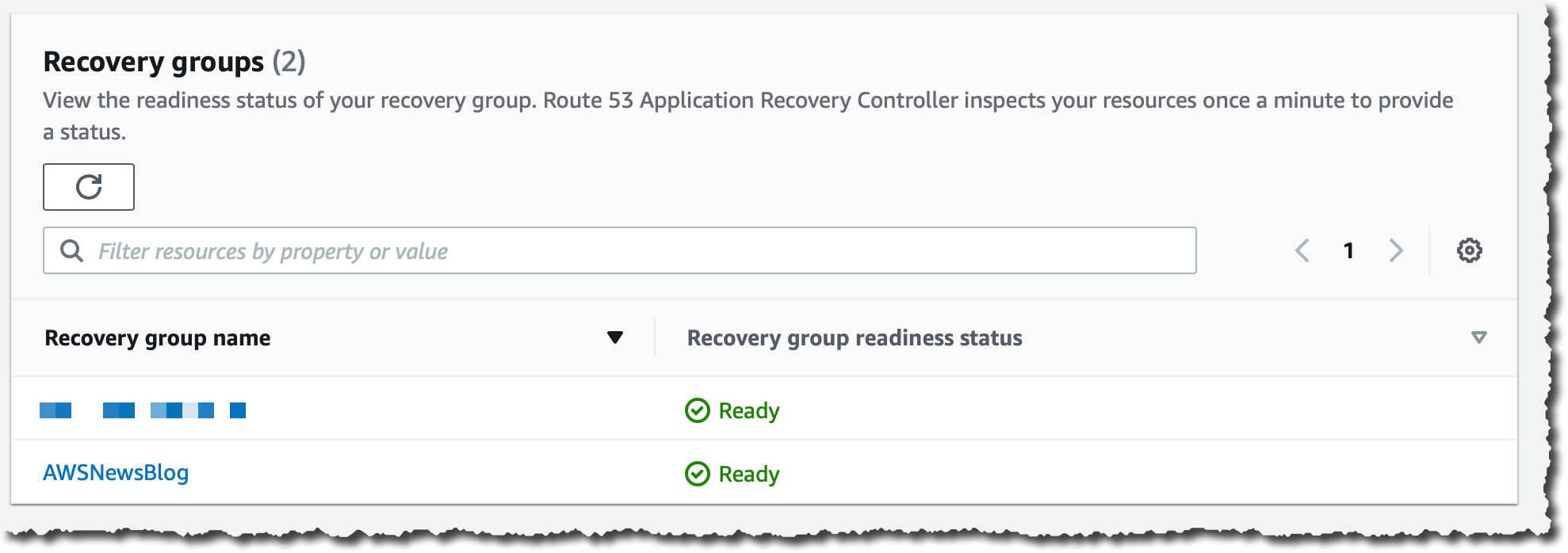
When all readiness checks in the group are green, the group has a status of Ready.
Now, I can configure and test the routing controls.
Terminology
Before I configure routing controls, let me share some basic terminology.
A cluster is a set of five redundant Regional endpoints against which you can execute API calls to update or get the state of routing controls. You can host multiple control panels and routing controls on one cluster.
A routing control is a simple on/off switch, hosted on a cluster, that you use to control routing of client traffic in and out of cells. When you create a routing control, you add a health check in Route 53 so that you can reroute traffic when you update the routing control in Route 53 Application Recovery Controller. The health checks must be associated with DNS failover records that front each application replica if you want to use them to route traffic with routing controls.
A control panel groups together a set of related routing controls.
Configure Routing Controls
I can use the Route 53 console or API actions to create a routing control for each AWS Region for my application. After I create routing controls, I create an Amazon Route 53 Application Recovery Controller health check for each one, and then associate each health check with a DNS failover record for my load balancers in each Region. Then, to fail over traffic between Regions, I change the routing control state for one routing control to off and another routing control state to on.
The first step is to create a cluster. A cluster is charged $2.5 / hour. When you create a cluster to experience Route 53 Application Recovery Controller, be sure to delete the cluster after your experimentation.

In the left navigation pane, I navigate to the cluster panel and then I choose Create.

I enter a name for my cluster and then choose Create cluster.
The cluster is in Pending state for a few minutes. After a while, its status changes to Deployed.
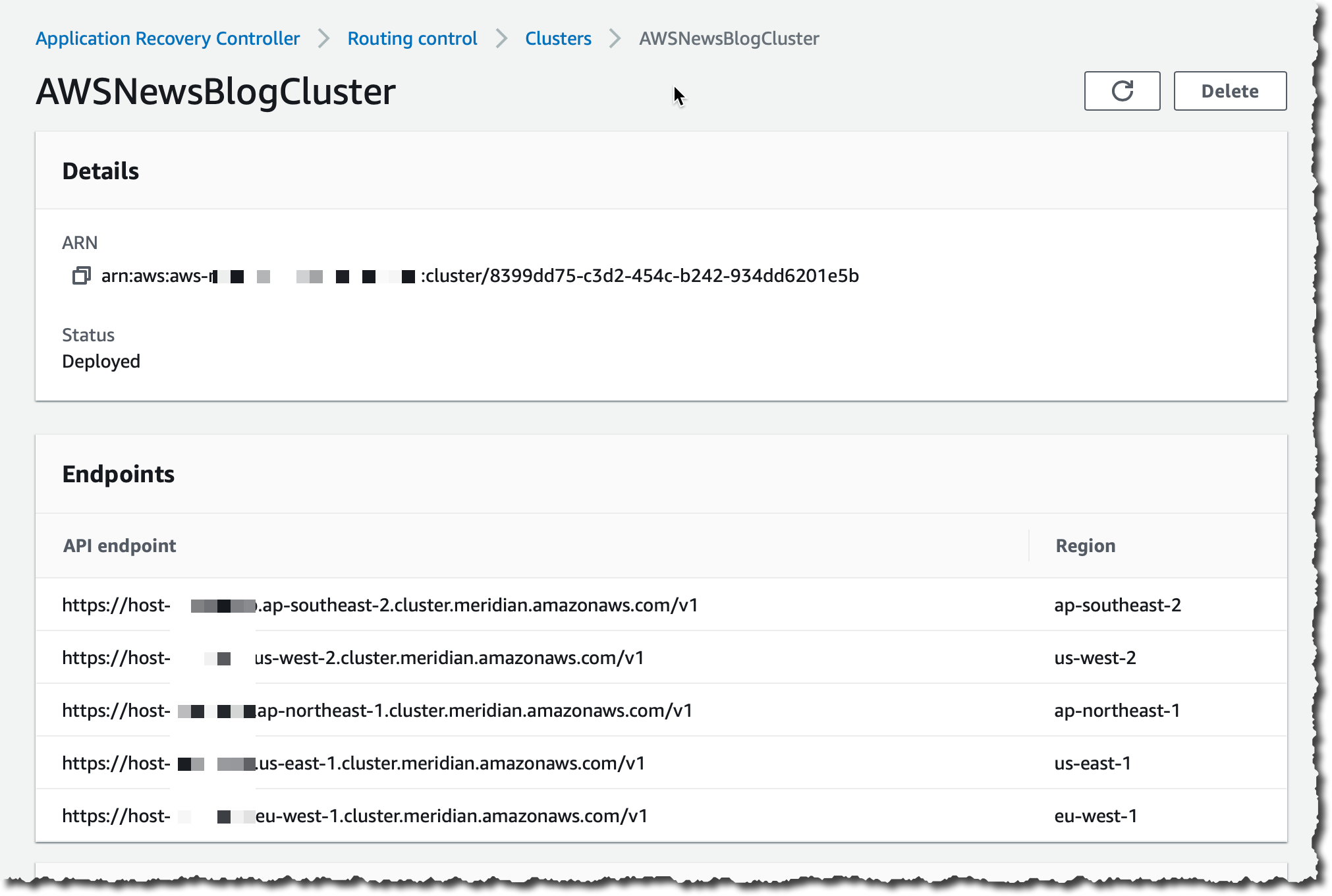
After it’s deployed, I select the cluster name to discover the five redundant API endpoints. You must specify one of those endpoints when you build recovery tools to retrieve or set routing control states. You can use any of the cluster endpoints, but in complex or automated scenarios, we recommend that your systems be prepared to retry with each of the available endpoints, using a different endpoint with each retry request.

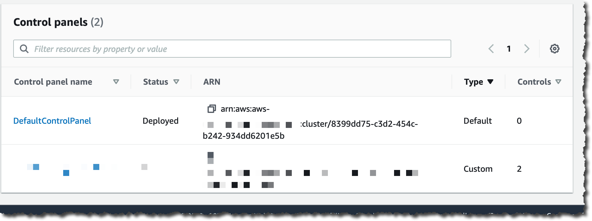
Traffic routing is managed through routing controls that are grouped in a control panel. You can create one or use the default one that is created for you.

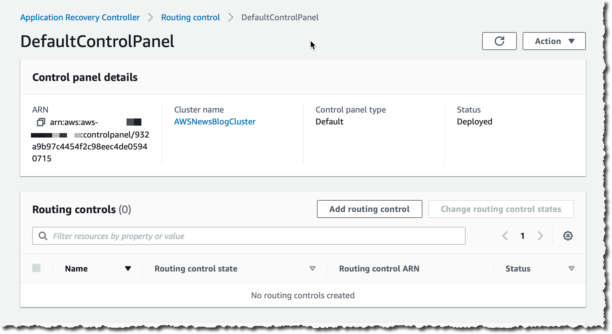
I choose DefaultControlPanel.

I choose Add routing control.

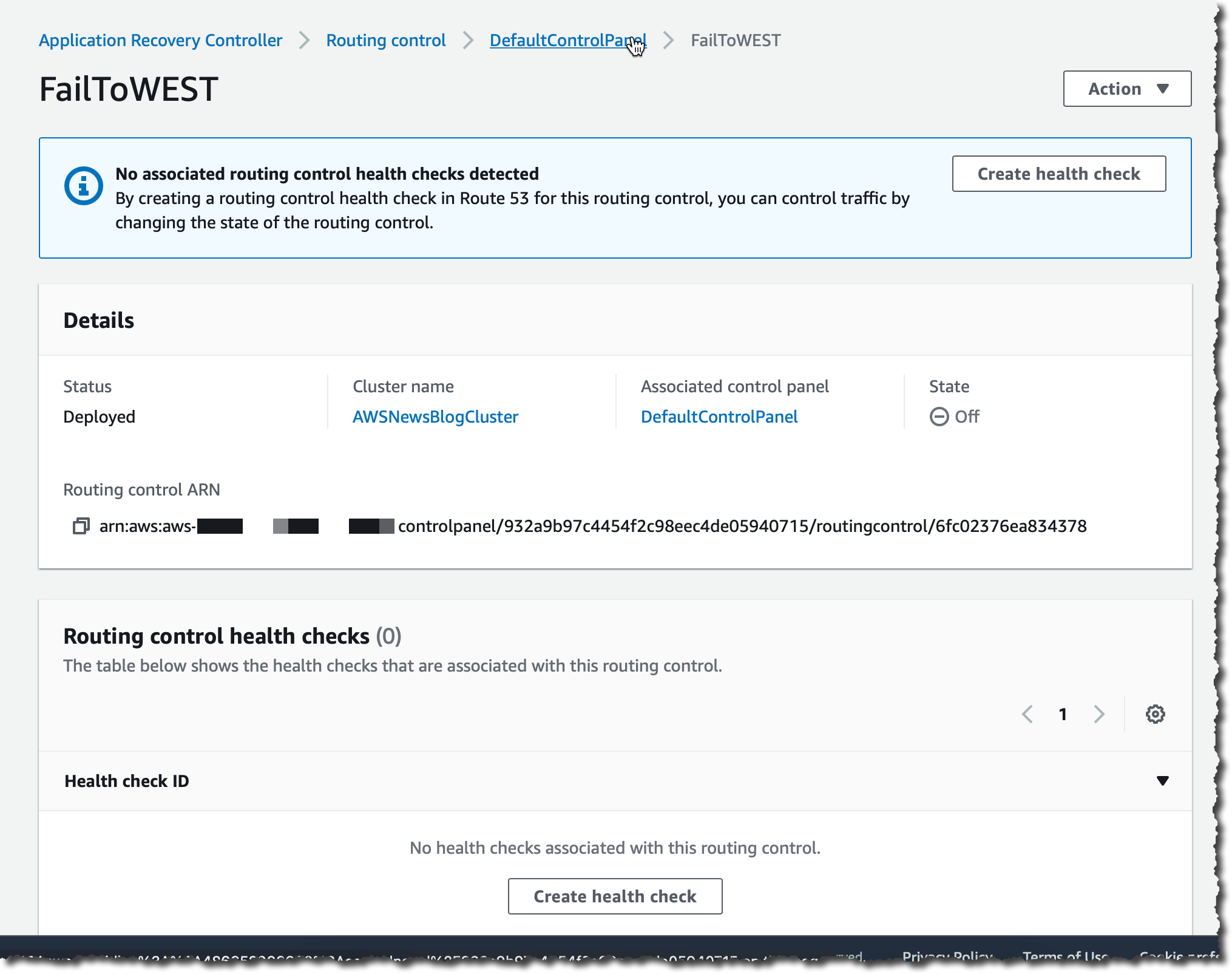
I enter a name for my routing (FailToWEST) control and then choose Create routing control. I repeat the operation for the second routing control (FailToEAST).

After the routing control is created, I choose it from the list. On the detail page, I choose Create health check to create a health check in Route 53.

I enter a name for the health check and then choose Create. I navigate to the Route 53 console to verify the health check was correctly created.
I create one health check for each routing control.
You might have noticed that the Control Panel provides a place where you can add Safety Rules. When you work with several routing controls at the same time, you might want some safeguards in place when you enable and disable them. These help you to avoid initiating a failover when a replica is not ready, or unintended consequences like turning both routing controls off and stopping all traffic flow. To create these safeguards, you create safety rules. For more information about safety rules, including usage examples, see the Route 53 Application Recovery Controller developer guide.
Now the routing controls and the DNS health check are in place, the last step is to route traffic to my application.
Adjust My DNS Settings
To route traffic to my application. I assign a DNS alias to the top-level entry point of the application in the cell. For this example, using the Route 53 console, I create two ALIAS A records of type FAILOVER and associate each health check with each DNS record. The two records have the same record name. One is the primary record and the other is the secondary record. For more information about Amazon Route 53 health checks, see the Amazon Route 53 developer guide.
On the application recovery routing controls page, I enable one of the two routing controls.

As soon as I do, all the traffic pointed to tictactoe.seb.go-aws.com goes to the infrastructure deployed on us-east-1.
Testing My Setup
To test my setup, I first use the dig command in a terminal. It shows the DNS CNAME record that points to the load balancer deployed in us-east-1.

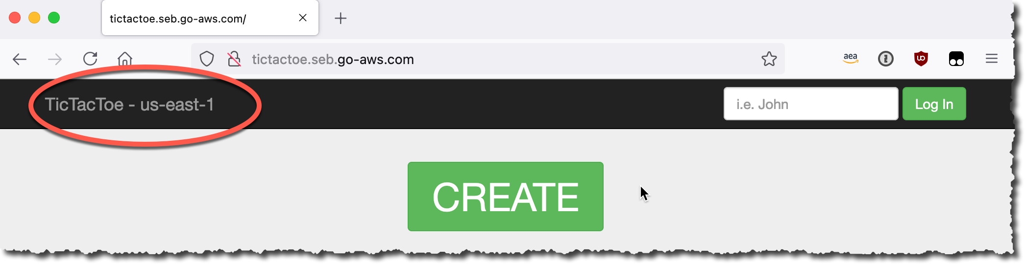
I also test the application with a web browser. I observe the name tictactoe.seb.go-aws.com goes to us-east-1.

Now, using the update-routing-control-state API action, the CLI, or the console, I turn off the routing control to the us-east-1 Region and turn on the one to the us-west-2 Region. When I use the CLI, I use the endpoints provided by my cluster.
aws route53-recovery-cluster update-routing-control-state \
     --routing-control-arn arn:aws:route53-recovery-control::012345678:controlpanel/xxx/routingcontrol/abcd \
     --routing-control-state On \
     --region us-west-2 \
     --endpoint-url https://host-xxx.us-west-2.cluster.routing-control.amazonaws.com/v1
In the console, I navigate to the control panel, I select the routing control I want to change and click Change routing control states.

After less than a minute, the DNS address is updated. My application traffic is now routed to the us-west-2 Region.

Readiness checks and routing controls provide a controlled failover for my application traffic, redirecting traffic from my active replica to my standby one, in another AWS Region. I can change the traffic routing manually, as I showed in the demo, or I can automate it using Amazon CloudWatch alarms based on technical and business metrics for my application.
Pricing
This new capability is charged on demand. There are no upfront costs. You are charged per readiness check and per cluster per hour. Readiness checks are charged $0.045 / hour. Cluster are charged $2.5 / hour. In the demo example used for this blog post, there are three readiness checks and one cluster. The price per hour for this setup, excluding the application itself, is 3 x $0.045 + 1 x $2.5 = $2.635 / hour. For more details about the pricing, including an example, see the Route 53 pricing page.
This new capability is a global service that can be used to monitor and control application recovery for application running in any of the public commercial AWS Regions. Give it a try and let us know what you think. As always, you can send feedback through your usual AWS Support contacts or post it on the AWS forum for Route 53 Application Recovery Controller.
— seb