Post Syndicated from Julian Wood original https://aws.amazon.com/blogs/compute/building-well-architected-serverless-applications-managing-application-security-boundaries-part-2/
This series uses the AWS Well-Architected Tool with the Serverless Lens to help customers build and operate applications using best practices. In each post, I address the nine serverless-specific questions identified by the Serverless Lens along with the recommended best practices. See the introduction post for a table of contents and explanation of the example application.
Security question SEC2: How do you manage your serverless application’s security boundaries?
This post continues part 1 of this security question. Previously, I cover how to evaluate and define resource policies, showing what policies are available for various serverless services. I show some of the features of AWS Web Application Firewall (AWS WAF) to protect APIs. Then then go through how to control network traffic at all layers. I explain how AWS Lambda functions connect to VPCs, and how to use private APIs and VPC endpoints. I walk through how to audit your traffic.
Required practice: Use temporary credentials between resources and components
Do not share credentials and permissions policies between resources to maintain a granular segregation of permissions and improve the security posture. Use temporary credentials that are frequently rotated and that have policies tailored to the access the resource needs.
Use dynamic authentication when accessing components and managed services
AWS Identity and Access Management (IAM) roles allows your applications to access AWS services securely without requiring you to manage or hardcode the security credentials. When you use a role, you don’t have to distribute long-term credentials such as a user name and password, or access keys. Instead, the role supplies temporary permissions that applications can use when they make calls to other AWS resources. When you create a Lambda function, for example, you specify an IAM role to associate with the function. The function can then use the role-supplied temporary credentials to sign API requests.
Use IAM for authorizing access to AWS managed services such as Lambda or Amazon S3. Lambda also assumes IAM roles, exposing and rotating temporary credentials to your functions. This enables your application code to access AWS services.
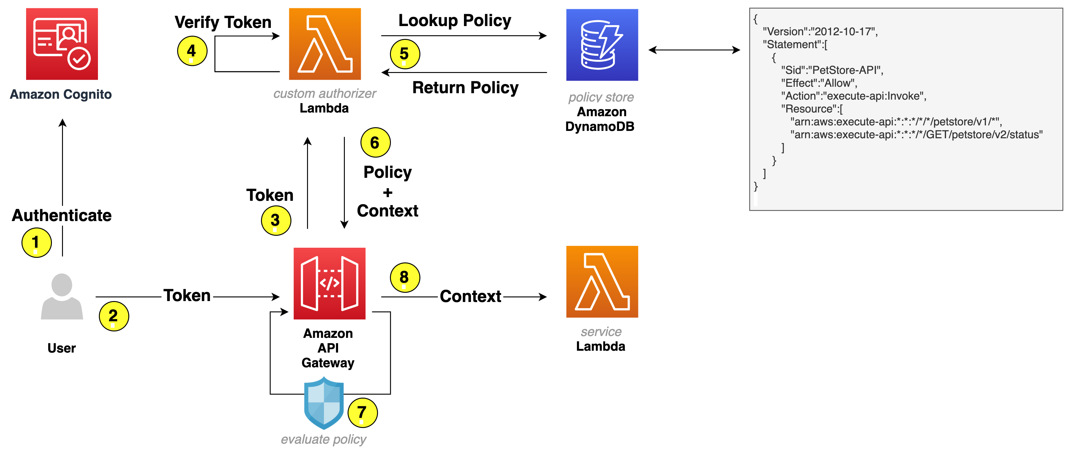
Use IAM to authorize access to internal or private Amazon API Gateway API consumers. See this list of AWS services that work with IAM.
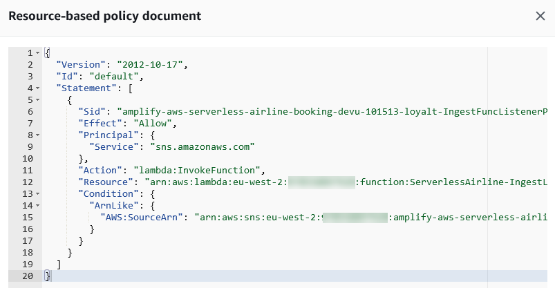
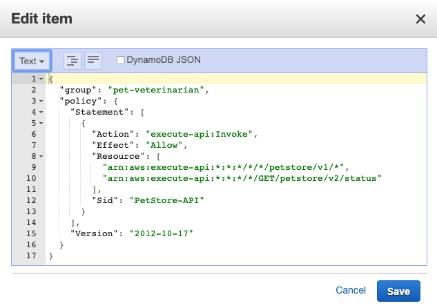
Within the serverless airline example used in this series, the loyalty service uses a Lambda function to fetch loyalty points and next tier progress. AWS AppSync acts as the client using an HTTP resolver, via an API Gateway REST API /loyalty/{customerId}/get resource, to invoke the function.
To ensure only AWS AppSync is authorized to invoke the API, IAM authorization is set within the API Gateway method request.

Viewing API Gateway IAM authorization
The IAM role specifies that appsync.amazonaws.com can perform an execute-api:Invoke on the specific API Gateway resource arn:aws:execute-api:${AWS::Region}:${AWS::AccountId}:${LoyaltyApi}/*/*/*
For more information, see “Using an IAM role to grant permissions to applications”.
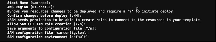
Use a framework such as the AWS Serverless Application Model (AWS SAM) to deploy your applications. This ensures that AWS resources are provisioned with unique per resource IAM roles. For example, AWS SAM automatically creates unique IAM roles for every Lambda function you create.
Best practice: Design smaller, single purpose functions
Creating smaller, single purpose functions enables you to keep your permissions aligned to least privileged access. This reduces the risk of compromise since the function does not require access to more than it needs.
Create single purpose functions with their own IAM role
Single purpose Lambda functions allow you to create IAM roles that are specific to your access requirements. For example, a large multipurpose function might need access to multiple AWS resources such as Amazon DynamoDB, Amazon S3, and Amazon Simple Queue Service (SQS). Single purpose functions would not need access to all of them at the same time.
With smaller, single purpose functions, it’s often easier to identify the specific resources and access requirements, and grant only those permissions. Additionally, new features are usually implemented by new functions in this architectural design. You can specifically grant permissions in new IAM roles for these functions.
Avoid sharing IAM roles with multiple cloud resources. As permissions are added to the role, these are shared across all resources using this role. For example, use one dedicated IAM role per Lambda function. This allows you to control permissions more intentionally. Even if some functions have the same policy initially, always separate the IAM roles to ensure least privilege policies.
Use least privilege access policies with your users and roles
When you create IAM policies, follow the standard security advice of granting least privilege, or granting only the permissions required to perform a task. Determine what users (and roles) must do and then craft policies that allow them to perform only those tasks.
Start with a minimum set of permissions and grant additional permissions as necessary. Doing so is more secure than starting with permissions that are too lenient and then trying to tighten them later. In the unlikely event of misused credentials, credentials will only be able to perform limited interactions.
To control access to AWS resources, AWS SAM uses the same mechanisms as AWS CloudFormation. For more information, see “Controlling access with AWS Identity and Access Management” in the AWS CloudFormation User Guide.
For a Lambda function, AWS SAM scopes the permissions of your Lambda functions to the resources that are used by your application. You add IAM policies as part of the AWS SAM template. The policies property can be the name of AWS managed policies, inline IAM policy documents, or AWS SAM policy templates.
For example, the serverless airline has a ConfirmBooking Lambda function that has UpdateItem permissions to the specific DynamoDB BookingTable resource.
Parameters:
    BookingTable:
        Type: AWS::SSM::Parameter::Value<String>
        Description: Parameter Name for Booking Table
Resources:
    ConfirmBooking:
        Type: AWS::Serverless::Function
        Properties:
            FunctionName: !Sub ServerlessAirline-ConfirmBooking-${Stage}
            Policies:
                - Version: "2012-10-17"
                  Statement:
                      Action: dynamodb:UpdateItem
                      Effect: Allow
                      Resource: !Sub "arn:${AWS::Partition}:dynamodb:${AWS::Region}:${AWS::AccountId}:table/${BookingTable}"
One of the fastest ways to scope permissions appropriately is to use AWS SAM policy templates. You can reference these templates directly in the AWS SAM template for your application, providing custom parameters as required.
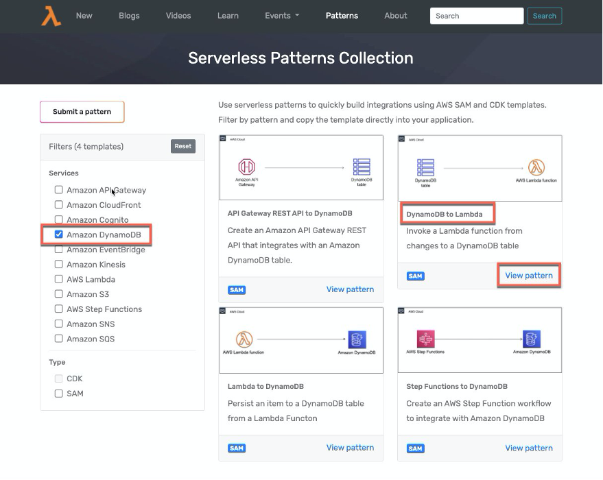
The serverless patterns collection allows you to build integrations quickly using AWS SAM and AWS Cloud Development Kit (AWS CDK) templates.
The booking service uses the SNSPublishMessagePolicy. This policy gives permission to the NotifyBooking Lambda function to publish a message to an Amazon Simple Notification Service (Amazon SNS) topic.
    BookingTopic:
        Type: AWS::SNS::Topic

    NotifyBooking:
        Type: AWS::Serverless::Function
        Properties:
            Policies:
                - SNSPublishMessagePolicy:
                      TopicName: !Sub ${BookingTopic.TopicName}
        …
Auditing permissions and removing unnecessary permissions
Audit permissions regularly to help you identify unused permissions so that you can remove them. You can use last accessed information to refine your policies and allow access to only the services and actions that your entities use. Use the IAM console to view when last an IAM role was used.

IAM last used
Use IAM access advisor to review when was the last time an AWS service was used from a specific IAM user or role. You can view last accessed information for IAM on the Access Advisor tab in the IAM console. Using this information, you can remove IAM policies and access from your IAM roles.

IAM access advisor
When creating and editing policies, you can validate them using IAM Access Analyzer, which provides over 100 policy checks. It generates security warnings when a statement in your policy allows access AWS considers overly permissive. Use the security warning’s actionable recommendations to help grant least privilege. To learn more about policy checks provided by IAM Access Analyzer, see “IAM Access Analyzer policy validation”.
With AWS CloudTrail, you can use CloudTrail event history to review individual actions your IAM role has performed in the past. Using this information, you can detect which permissions were actively used, and decide to remove permissions.
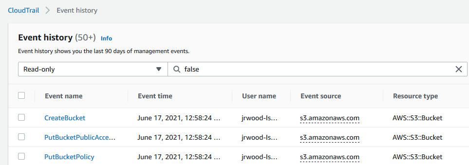
AWS CloudTrail
To work out which permissions you may need, you can generate IAM policies based on access activity. You configure an IAM role with broad permissions while the application is in development. Access Analyzer reviews your CloudTrail logs. It generates a policy template that contains the permissions that the role used in your specified date range. Use the template to create a policy that grants only the permissions needed to support your specific use case. For more information, see “Generate policies based on access activity”.

IAM Access Analyzer
Conclusion
Managing your serverless application’s security boundaries ensures isolation for, within, and between components. In this post, I continue from part 1, looking at using temporary credentials between resources and components. I cover why smaller, single purpose functions are better from a security perspective, and how to audit permissions. I show how to use AWS SAM to create per-function IAM roles.
For more serverless learning resources, visit https://serverlessland.com.


 Praveen Krishnamoorthy Ravikumar is a Data Architect with AWS Professional Services Intelligence Practice. He helps customers implement big data and analytics platform and solutions.
 Abhishek Gupta is a Data and ML Engineer with AWS Professional Services Practice.
 Ashok Yoganand Sridharan is a Big Data Consultant with AWS Professional Services Intelligence Practice. He helps customers implement big data and analytics platform and solutions


 Dhiraj Thakur is a Solutions Architect with Amazon Web Services. He works with AWS customers and partners to guide enterprise cloud adoption, migration, and strategy. He is passionate about technology and enjoys building and experimenting in the analytics and AI/ML space.
 Saurabh Shrivastava is a solutions architect leader and analytics/ML specialist working with global systems integrators. He works with AWS Partners and customers to provide them with architectural guidance for building scalable architecture in hybrid and AWS environments. He enjoys spending time with his family outdoors and traveling to new destinations to discover new cultures.
 Dylan Qu is an AWS solutions architect responsible for providing architectural guidance across the full AWS stack with a focus on data analytics, AI/ML, and DevOps.


 Sameer Goel is a solutions architect in Seattle who drives customers’ success by building prototypes on cutting-edge initiatives. Prior to joining AWS, Sameer graduated with a Master’s degree with a Data Science concentration from NEU Boston. He enjoys building and experimenting with creative projects and applications.
 Pratik Patel is a senior technical account manager and streaming analytics specialist. He works with AWS customers and provides ongoing support and technical guidance to help plan and build solutions by using best practices, and proactively helps keep customers’ AWS environments operationally healthy.