Post Syndicated from Daniel Rozo original https://aws.amazon.com/blogs/big-data/enrich-datasets-for-descriptive-analytics-with-aws-glue-databrew/
Data analytics remains a constantly hot topic. More and more businesses are beginning to understand the potential their data has to allow them to serve customers more effectively and give them a competitive advantage. However, for many small to medium businesses, gaining insight from their data can be challenging because they often lack in-house data engineering skills and knowledge.
Data enrichment is another challenge. Businesses that focus on analytics using only their internal datasets miss the opportunity to gain better insights by using reliable and credible public datasets. Small to medium businesses are no exception to this shortcoming, where obstacles such as not having sufficient data diminish their ability to make well-informed decisions based on accurate analytical insights.
In this post, we demonstrate how AWS Glue DataBrew enables businesses of all sizes to get started with data analytics with no prior coding knowledge. DataBrew is a visual data preparation tool that makes it easy for data analysts and scientists to clean and normalize data in preparation for analytics or machine learning. It includes more than 350 pre-built transformations for common data preparation use cases, enabling you to get started with cleaning, preparing, and combining your datasets without writing code.
For this post, we assume the role of a fictitious small Dutch solar panel distribution and installation company named OurCompany. We demonstrate how this company can prepare, combine, and enrich an internal dataset with publicly available data from the Dutch public entity, the Centraal Bureau voor de Statistiek (CBS), or in English, Statistics Netherlands. Ultimately, OurCompany desires to know how well they’re performing compared to the official reported values by the CBS across two important key performance indicators (KPIs): the amount of solar panel installations, and total energy capacity in kilowatt (kW) per region.
Solution overview
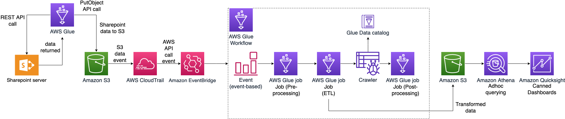
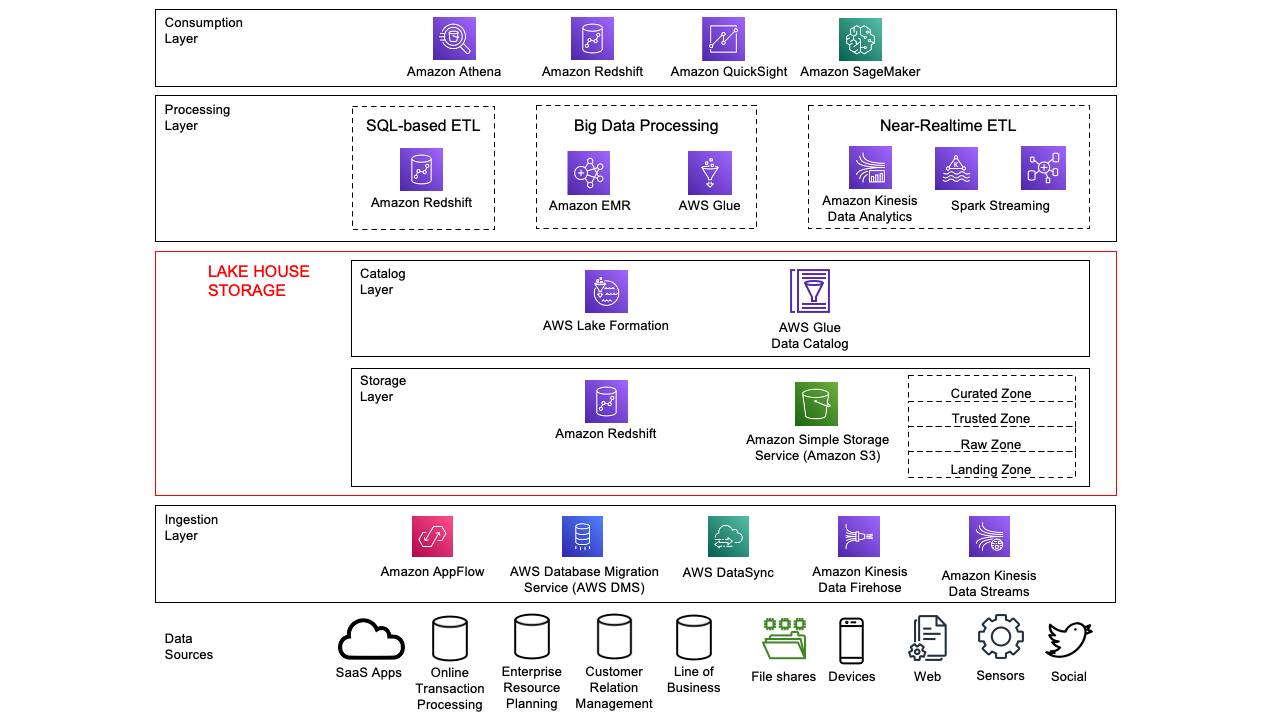
The architecture uses DataBrew for data preparation and transformation, Amazon Simple Storage Service (Amazon S3) as the storage layer of the entire data pipeline, and the AWS Glue Data Catalog for storing the dataset’s business and technical metadata. Following the modern data architecture best practices, this solution adheres to foundational logical layers of the Lake House Architecture.
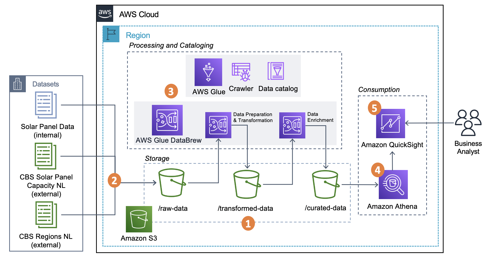
The solution includes the following steps:
- We set up the storage layer using Amazon S3 by creating the following folders:
raw-data,transformed-data, andcurated-data. We use these folders to track the different stages of our data pipeline consumption readiness. - Three CSV raw data files containing unprocessed data of solar panels as well as the external datasets from the CBS are ingested into the
raw-dataS3 folder. - This part of the architecture incorporates both processing and cataloging capabilities:
- We use AWS Glue crawlers to populate the initial schema definition tables for the raw dataset automatically. For the remaining two stages of the data pipeline (
transformed-dataandcurated-data), we utilize the functionality in DataBrew to directly create schema definition tables into the Data Catalog. Each table provides an up-to-date schema definition of the datasets we store on Amazon S3. - We work with DataBrew projects as the centerpiece of our data analysis and transformation efforts. In here, we set up no-code data preparation and transformation steps, and visualize them through a highly interactive, intuitive user interface. Finally, we define DataBrew jobs to apply these steps and store transformation outputs on Amazon S3.
- We use AWS Glue crawlers to populate the initial schema definition tables for the raw dataset automatically. For the remaining two stages of the data pipeline (
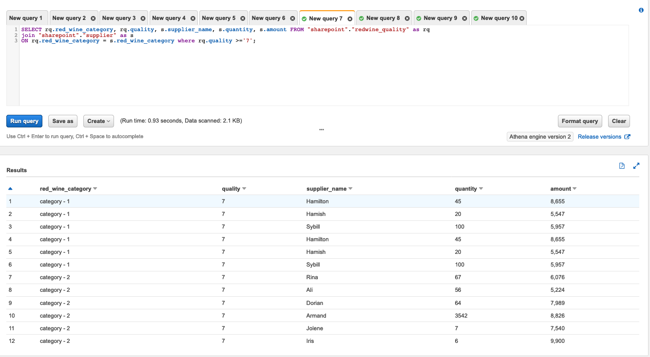
- To gain the benefits of granular access control and easily visualize data from Amazon S3, we take advantage of the seamless integration between Amazon Athena and Amazon QuickSight. This provides a SQL interface to query all the information we need from the curated dataset stored on Amazon S3 without the need to create and maintain manifest files.
- Finally, we construct an interactive dashboard with QuickSight to depict the final curated dataset alongside our two critical KPIs.
Prerequisites
Before beginning this tutorial, make sure you have the required Identity and Access Management (IAM) permissions to create the resources required as part of the solution. Your AWS account should also have an active subscription to QuickSight to create the visualization on processed data. If you don’t have a QuickSight account, you can sign up for an account.
The following sections provide a step-by-step guide to create and deploy the entire data pipeline for OurCompany without the use of code.
Data preparation steps
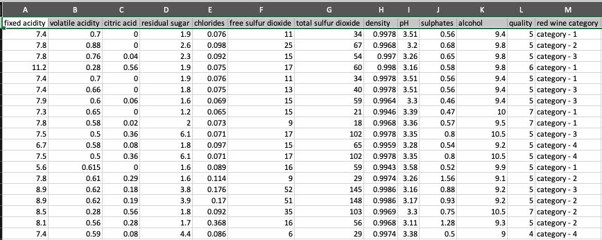
We work with the following files:
- CBS Dutch municipalities and provinces (Gemeentelijke indeling op 1 januari 2021) – Holds all the municipalities and provinces names and codes of the Netherlands. Download the file
gemeenten alfabetisch 2021. Open the file and save it ascbs_regions_nl.csv. Remember to change the format to CSV (comma-delimited). - CBS Solar power dataset (Zonnestroom; vermogen bedrijven en woningen, regio, 2012-2018) – This file contains the installed capacity in kilowatts and total number of installations for businesses and private homes across the Netherlands from 2012–2018. To download the file, go to the dataset page, choose the
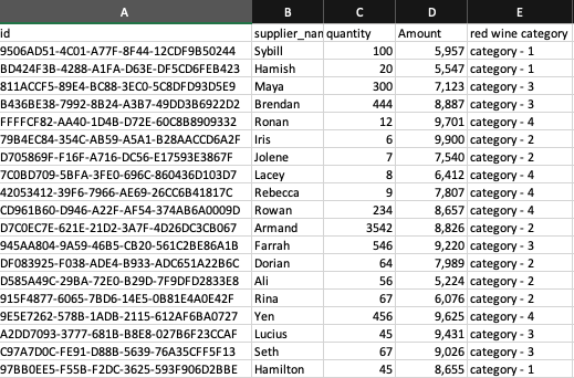
Onbewerkte dataset, and download the CSV file. Rename the file tocbs_sp_cap_nl.csv. - OurCompany’s solar panel historical data – Contains the reported energy capacity from all solar panel installations of OurCompany across the Netherlands from 2012 until 2018. Download the file.
As a result, the following are the expected input files we use to work with the data analytics pipeline:
cbs_regions_nl.csvcbs_sp_cap_nl.csvsp_data.csv
Set up the storage Layer
We first need to create the storage layer for our solution to store all raw, transformed, and curated datasets. We use Amazon S3 as the storage layer of our entire data pipeline.
- Create an S3 bucket in the AWS Region where you want to build this solution. In our case, the bucket is named
cbs-solar-panel-data. You can use the same name followed by a unique identifier.

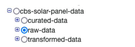
- Create the following three prefixes (folders) in your S3 bucket by choosing Create folder:
curated-data/raw-data/transformed-data/

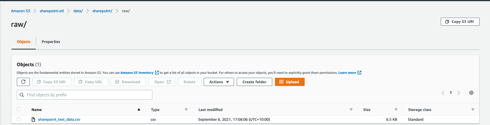
- Upload the three raw files to the
raw-data/prefix. - Create two prefixes within the
transformed-data/prefix namedcbs_data/andsp_data/.


Create a Data Catalog database
After we set up the storage layer of our data pipeline, we need to create the Data Catalog to store all the metadata of the datasets hosted in Amazon S3. To do so, follow these steps:
- Open the AWS Glue console in the same Region of your newly created S3 bucket.
- In the navigation pane, choose Databases.
- Choose Add database.
- Enter the name for the Data Catalog to store all the dataset’s metadata.
- Name the database
sp_catalog_db.
Create AWS Glue data crawlers
Now that we created the catalog database, it’s time to crawl the raw data prefix to automatically retrieve the metadata associated to each input file.
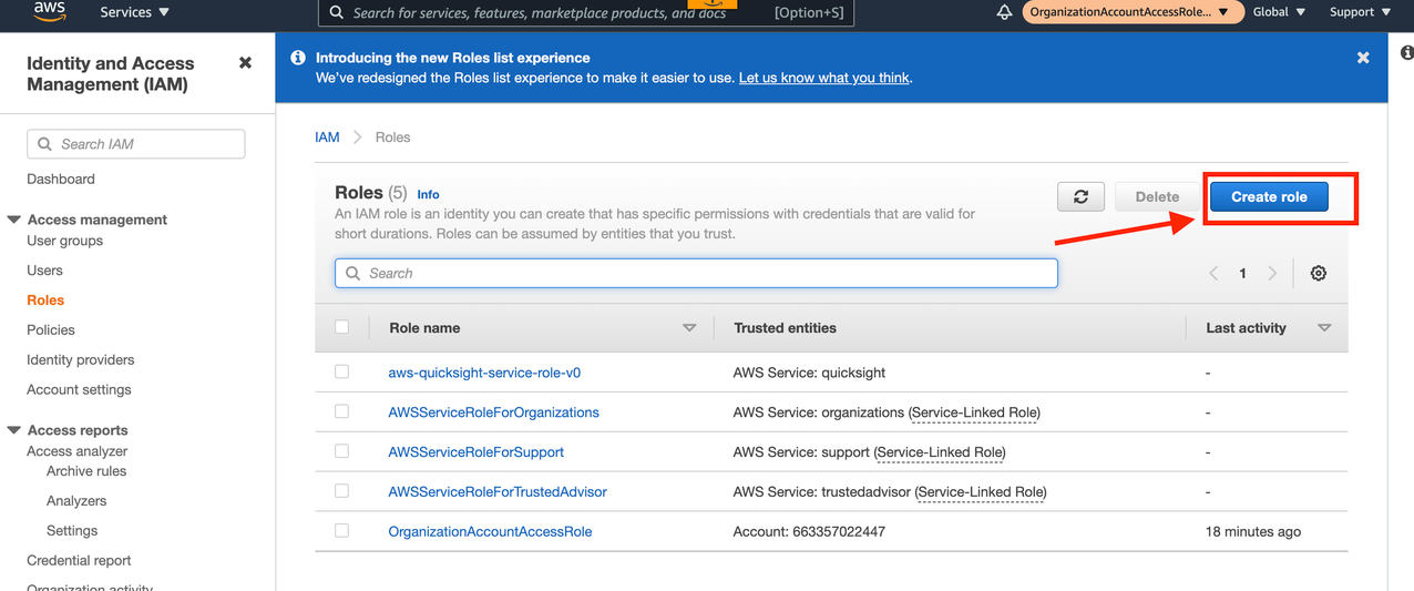
- On the AWS Glue console, choose Crawlers in the navigation pane.
- Add a crawler with the name
crawler_rawand choose Next. - For S3 path, select the
raw-datafolder of thecbs-solar-panel-dataprefix.

- Create an IAM role and name it
AWSGlueServiceRole-cbsdata. - Leave the frequency as Run on demand.
- Choose the
sp_catalog_dbdatabase created in the previous section, and enter the prefixraw_to identify the tables that belong to the raw data folder. - Review the parameters of the crawler and then choose Finish.
- After the crawler is created, select it and choose Run crawler.
After successful deployment of the crawler, your three tables are created in the sp_catalog_db database: raw_sp_data_csv, raw_cbs_regions_nl_csv, and raw_cbs_sp_cap_nl_csv.

Create DataBrew raw datasets
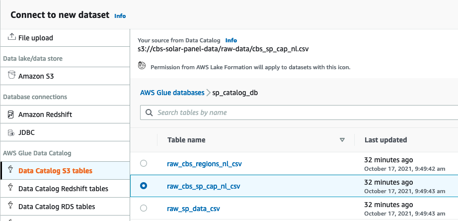
To utilize the power of DataBrew, we need to connect datasets that point to the Data Catalog S3 tables we just created. Follow these steps to connect the datasets:
- On the DataBrew console, choose Datasets in the navigation pane.
- Choose Connect new dataset.
- Name the dataset
cbs-sp-cap-nl-dataset. - For Connect to new dataset, choose Data Catalog S3 tables.
- Select the
sp_catalog_dbdatabase and theraw_cbs_sp_cap_nl_csvtable.

- Choose Create dataset.
We need to create to two more datasets following the same process. The following table summarizes the names and tables of the catalog required for the new datasets.
| Dataset name | Data catalog table |
sp-dataset |
raw_sp_data_csv |
cbs-regions-nl-dataset |
raw_cbs_regions_nl_csv |
Import DataBrew recipes
A recipe is a set of data transformation steps. These transformations are applied to one or multiple datasets of your DataBrew project. For more information about recipes, see Creating and using AWS Glue DataBrew recipes.
We have prepared three DataBrew recipes, which contain the set of data transformation steps we need for this data pipeline. Some of these transformation steps include: renaming columns (from Dutch to English), removing null or missing values, aggregating rows based on specific attributes, and combining datasets in the transformation stage.
To import the recipes, follow these instructions:
- On the DataBrew console, choose Recipes in the navigation pane.
- Choose Upload recipe.
- Enter the name of the recipe:
recipe-1-transform-cbs-data. - Upload the following JSON recipe.
- Choose Create recipe.
Now we need to upload two more recipes that we use for transformation and aggregation projects in DataBrew.
- Follow the same procedure to import the following recipes:
| Recipe name | Recipe source file |
recipe-2-transform-sp-data |
Download |
recipe-3-curate-sp-cbs-data |
Download |
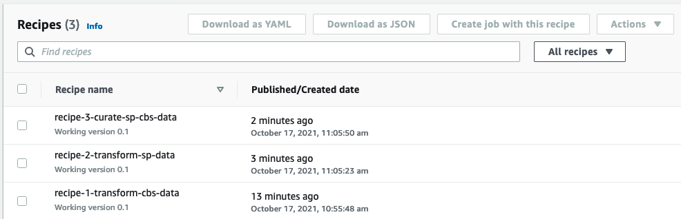
- Make sure the recipes are listed in the Recipes section filtered by All recipes.

Set up DataBrew projects and jobs
After we successfully create the Data Catalog database, crawlers, DataBrew datasets, and import the DataBrew recipes, we need to create the first transformation project.
CBS external data transformation project
The first project takes care of transforming, cleaning, and preparing cbs-sp-cap-nl-dataset. To create the project, follow these steps:
- On the DataBrew console, choose Projects in the navigation pane.
- Create a new project with the name
1-transform-cbs-data. - In the Recipe details section, choose Edit existing recipe and choose the recipe
recipe-1-transform-cbs-data.

- Select the newly created
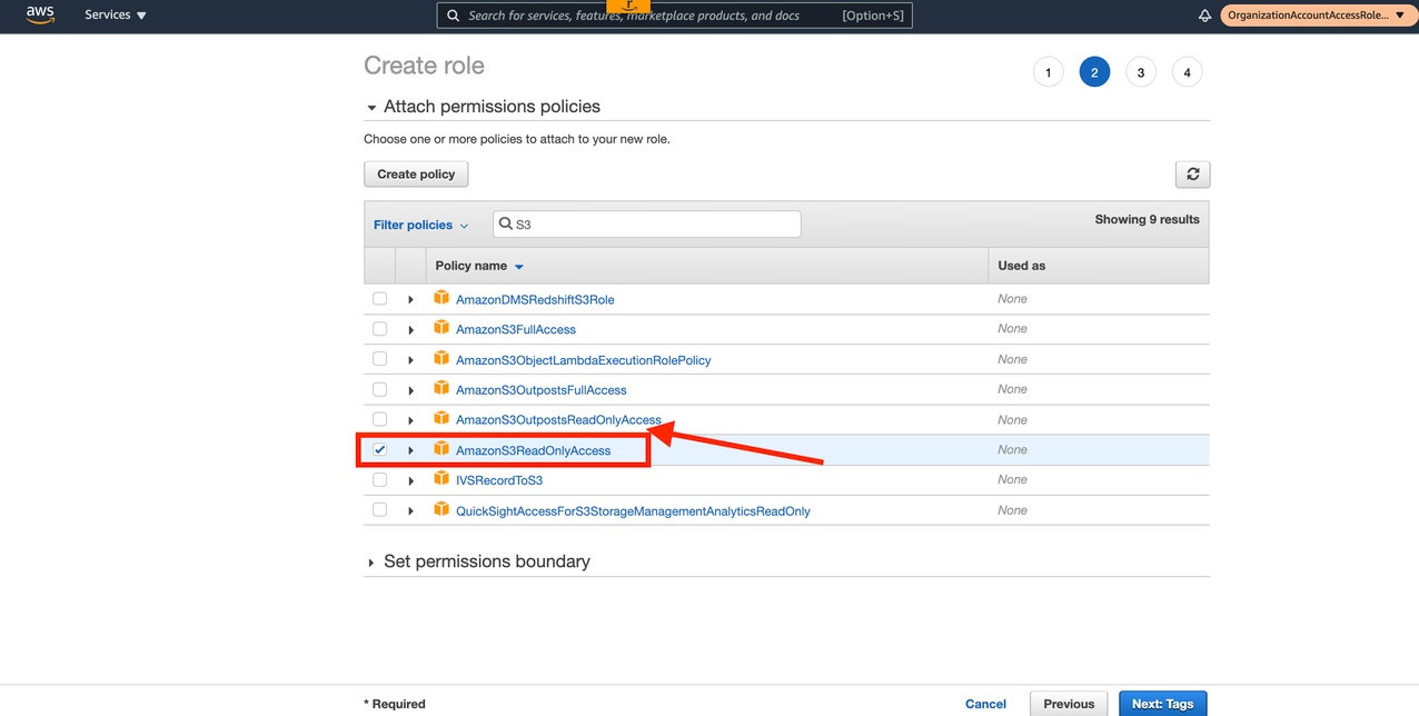
cbs-sp-cap-nl-datasetunder Select a dataset. - In the Permissions section, choose Create a new IAM role.
- As suffix, enter
sp-project. - Choose Create project.

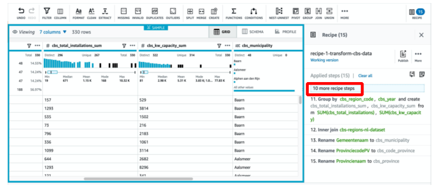
After you create the project, a preview dataset is displayed as a result of applying the selected recipe. When you choose 10 more recipe steps, the service shows the entire set of transformation steps.
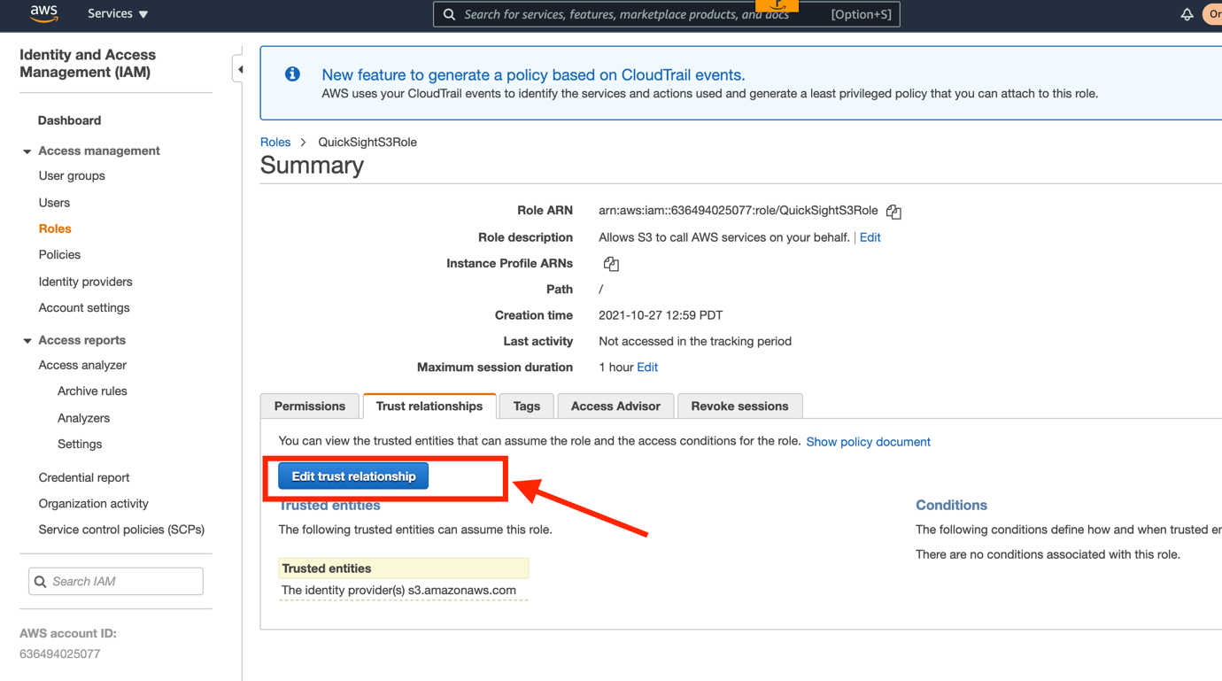
After you create the project, you need to grant put and delete S3 object permissions to the created role AWSGlueDataBrewServiceRole-sp-project on IAM. Add an inline policy using the following JSON and replace the resource with your S3 bucket name:
This role also needs permissions to access the Data Catalog. To grant these permissions, add the managed policy AWSGlueServiceRole to the role.
CBS external data transformation job
After we define the project, we need to configure and run a job to apply the transformation across the entire raw dataset stored in the Raw-data folder of your S3 bucket. To do so, you need to do the following:
- On the DataBrew project page, choose Create job.
- For Job name, enter
1-transform-cbs-data-job. - For Output to, choose Data Catalog S3 tables.
- For File type¸ choose Parquet.
- For Database name, choose
sp_catalog_db. - For Table name, choose Create new table.
- For Catalog table name, enter
transformed_cbs_data. - For S3 location, enter
s3://<your-S3-bucket-name>/transformed-data/cbs_data/.

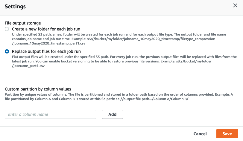
- In the job output settings section, choose Settings.
- Select Replace output files for each job run and then choose Save.

- In the permissions section, choose the automatically created role with the
sp-projectsuffix; for example,AWSGlueDataBrewServiceRole-sp-project. - Review the job details once more and then choose Create and run job.
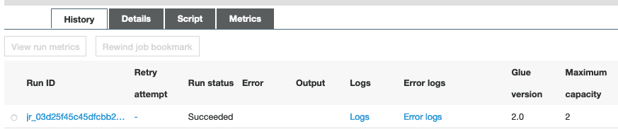
- Back in the main project view, choose Job details.

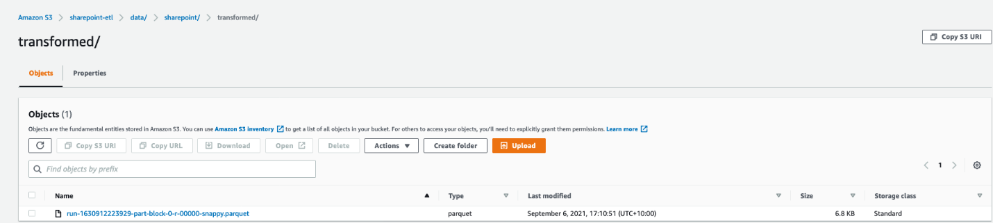
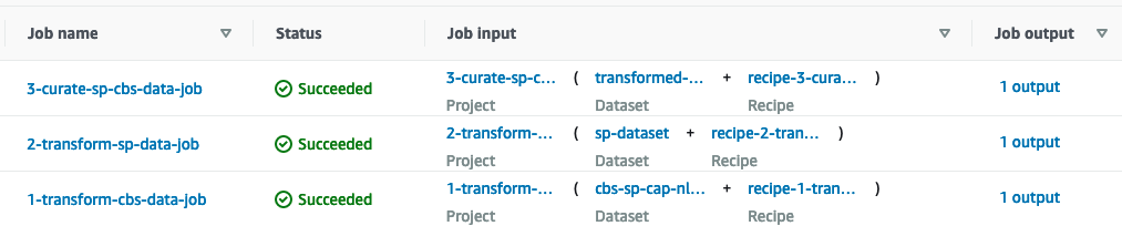
After a few minutes, the job status changes from Running to Successful. Choose the output to go to the S3 location where all the generated Parquet files are stored.
Solar panels data transformation stage
We now create the second phase of the data pipeline. We create a project and a job using the same procedure described in the previous section.
- Create a DataBrew project with the following parameters:
- Project name –
2-transform-sp-data - Imported recipe –
recipe-2-transform-sp-data - Dataset –
sp_dataset - Permissions role –
AWSGlueDataBrewServiceRole-sp-project
- Project name –
- Create and run another DataBrew job with the following parameters:
- Job name –
2-transform-sp-data-job - Output to – Data Catalog S3 tables
- File type – Parquet
- Database name –
sp_catalog_db - Create new table with table name –
transformed_sp_data - S3 location –
s3://<your-S3-bucket-name>/transformed-data/sp_data/ - Settings – Replace output files for each job run.
- Permissions role –
AWSGlueDataBrewServiceRole-sp-project
- Job name –
- After the job is complete, create the DataBrew datasets with the following parameters:
| Dataset name | Data catalog table |
transformed-cbs-dataset |
awsgluedatabrew_transformed_cbs_data |
transformed-sp-dataset |
awsgluedatabrew_transformed_sp_data |
You should now see five items as part of your DataBrew dataset.

Data curation and aggregation stage
We now create the final DataBrew project and job.
- Create a DataBrew project with the following parameters:
- Project name –
3-curate-sp-cbs-data - Imported recipe –
recipe-3-curate-sp-cbs-data - Dataset –
transformed_sp_dataset - Permissions role –
AWSGlueDataBrewServiceRole-sp-project
- Project name –
- Create a DataBrew job with the following parameters:
- Job name –
3-curate-sp-cbs-data-job - Output to – Data Catalog S3 tables
- File type – Parquet
- Database name –
sp_catalog_db - Create new table with table name –
curated_data - S3 location –
s3://<your-S3-bucket-name>/curated-data/ - Settings – Replace output files for each job run
- Permissions role –
AWSGlueDataBrewServiceRole-sp-project
- Job name –
The last project defines a single transformation step; the join between the transformed-cbs-dataset and the transformed-sp-dataset based on the municipality code and the year.
The DataBrew job should take a few minutes to complete.
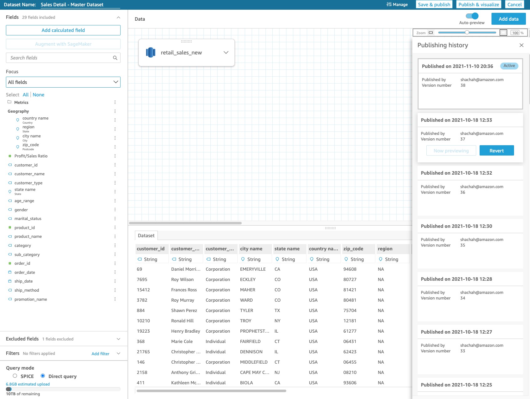
Next, check your sp_catalog_db database. You should now have raw, transformed, and curated tables in your database. DataBrew automatically adds the prefix awsgluedatabrew_ to both the transformed and curated tables in the catalog.

Consume curated datasets for descriptive analytics
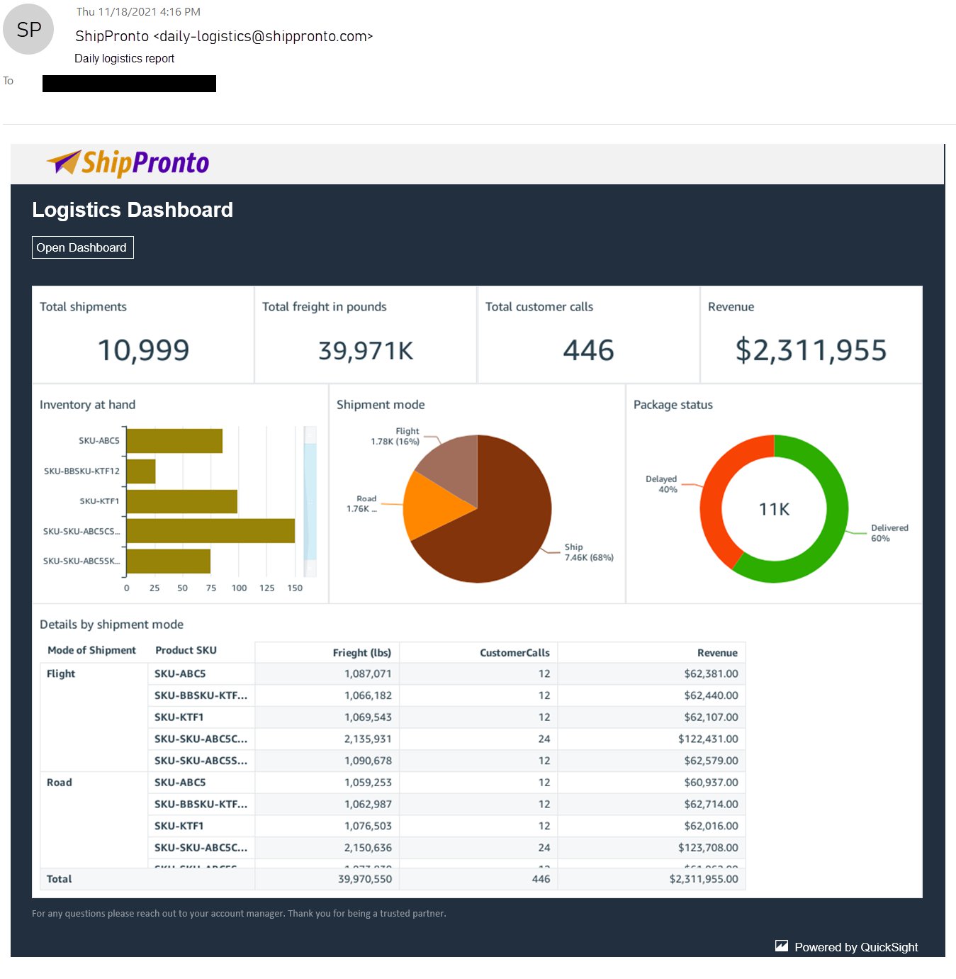
We’re now ready to build the consumption layer for descriptive analytics with QuickSight. In this section, we build a business intelligence dashboard that reflects OurCompany’s solar panel energy capacity and installations participation in contrast to the reported values by the CBS from 2012–2018.
To complete this section, you need to have the default primary workgroup already set up on Athena in the same Region where you implemented the data pipeline. If it’s your first time setting up workgroups on Athena, follow the instructions in Setting up Workgroups.
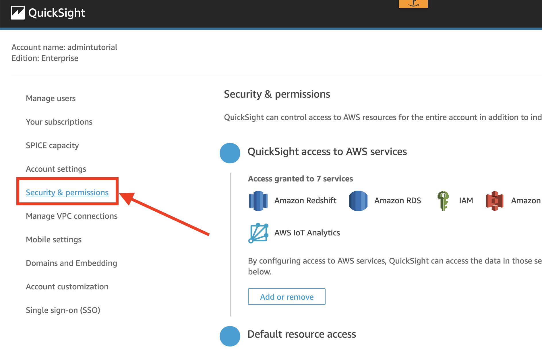
Also make sure that QuickSight has the right permissions to access Athena and your S3 bucket. Then complete the following steps:
- On the QuickSight console, choose Datasets in the navigation pane.
- Choose Create a new dataset.
- Select Athena as the data source.
- For Data source name, enter
sp_data_source. - Choose Create data source.

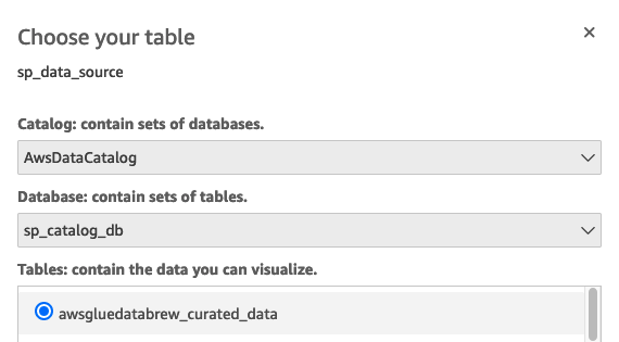
- Choose
AWSDataCatalogas the catalog andsp_catalog_dbas the database. - Select the table
curated_data. - Choose Select.

- In the Finish dataset creation section, choose Directly query your data and choose Visualize.
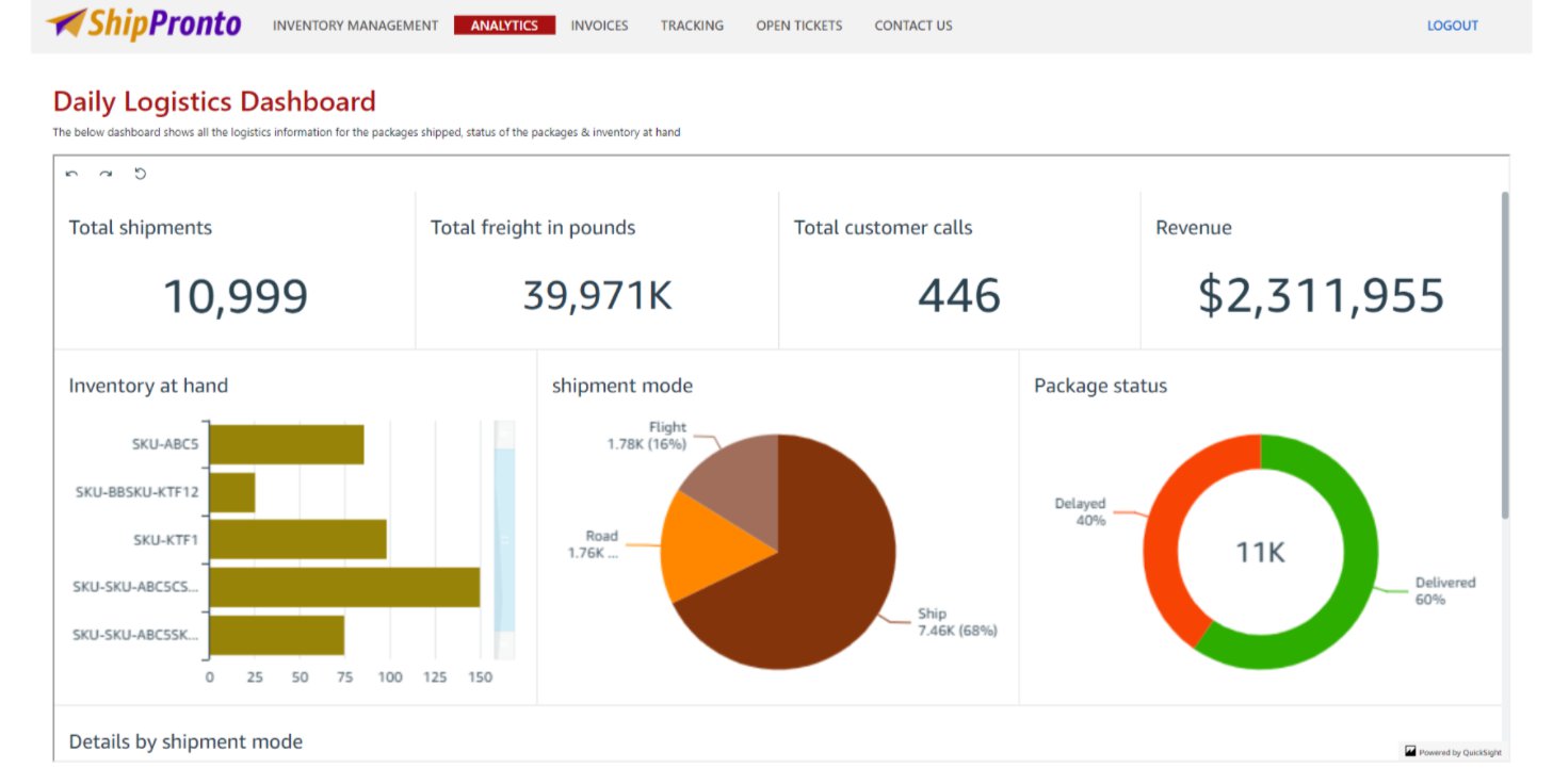
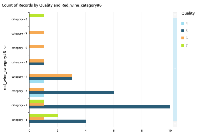
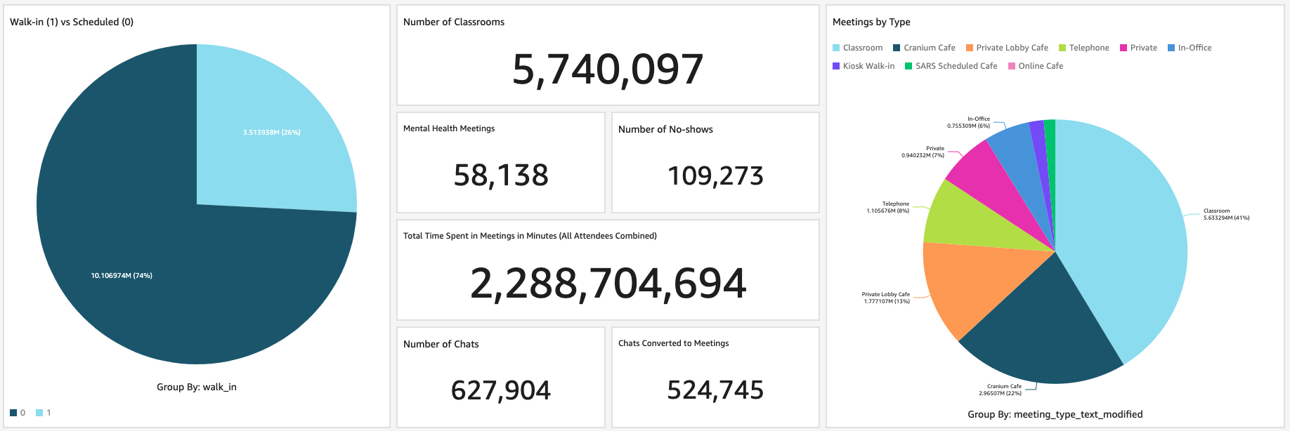
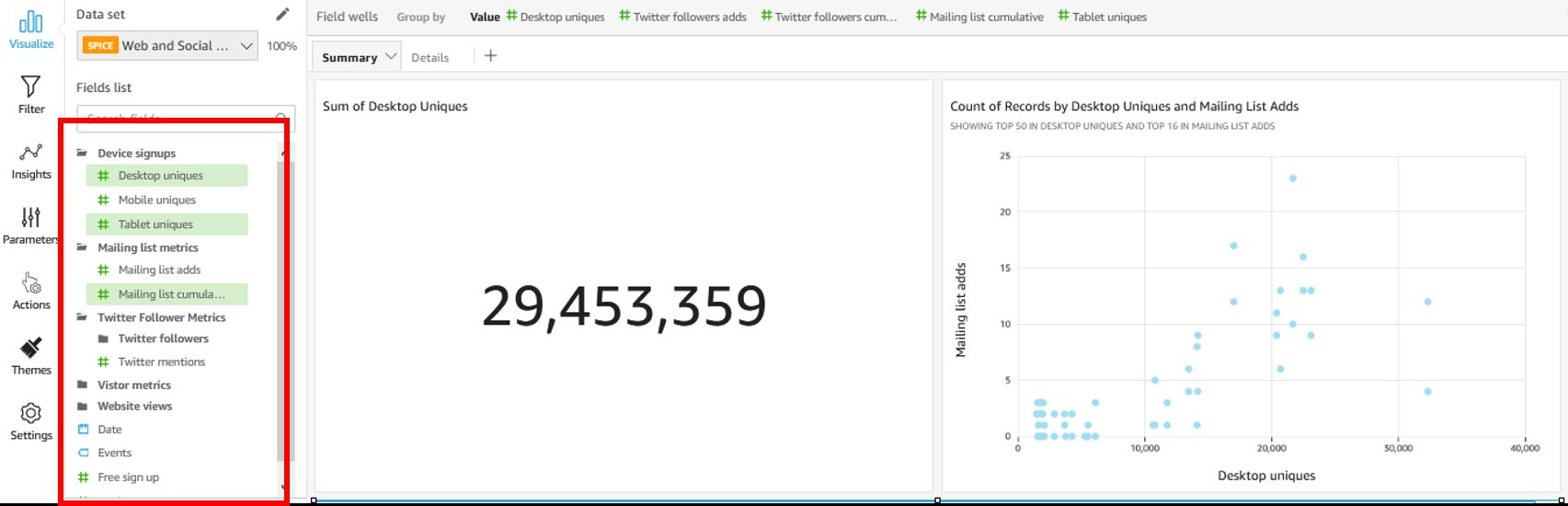
- Choose the clustered bar combo chart from the Visual types list.
- Expand the field wells section and then drag and drop the following fields into each section as shown in the following screenshot.

- Rename the visualization as you like, and optionally filter the report by
sp_yearusing the Filter option.

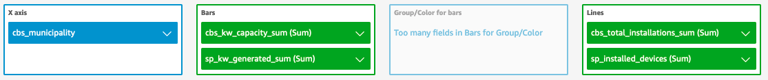
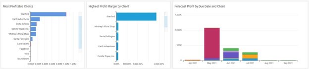
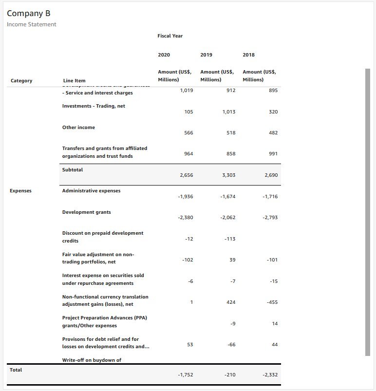
From this graph, we can already benchmark OurCompany against the regional values reported by the CBS across two dimensions: the total amount of installations and the total kW capacity generated by solar panels.
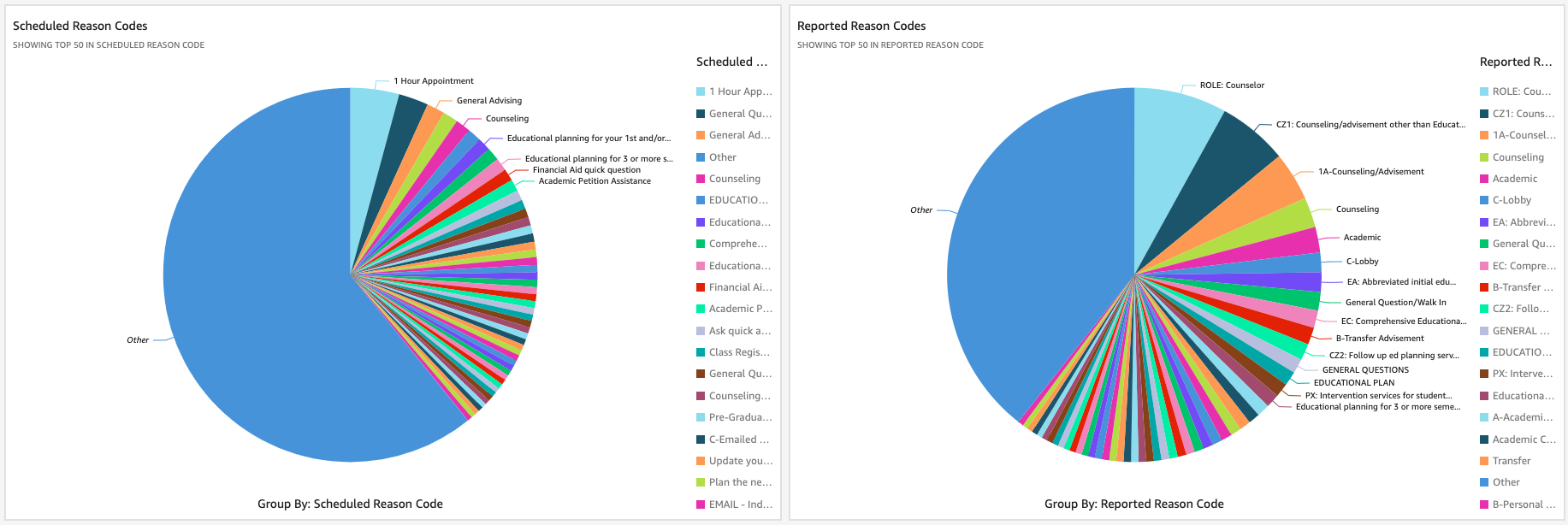
We went one step further and created two KPI visualizations to empower our descriptive analytics capabilities. The following is our final dashboard that we can use to enhance our decision-making process.

Clean up resources
To clean all the resources we created for the data pipeline, complete the following steps:
- Remove the QuickSight analyses you created.
- Delete the dataset
curated_data. - Delete all the DataBrew projects with their associated recipes.
- Delete all the DataBrew datasets.
- Delete all the AWS Glue crawlers you created.
- Delete the
sp_catalog_dbcatalog database; this removes all the tables. - Empty the contents of your S3 bucket and delete it.
Conclusion
In this post, we demonstrated how you can begin your data analytics journey. With DataBrew, you can prepare and combine the data you already have with publicly available datasets such as those from the Dutch CBS (Centraal Bureau voor de Statistiek) without needing to write a single line of code. Start using DataBrew today and enrich key datasets in AWS for enhanced descriptive analytics capabilities.
About the Authors
 Daniel Rozo is a Solutions Architect with Amazon Web Services based out of Amsterdam, The Netherlands. He is devoted to working with customers and engineering simple data and analytics solutions on AWS. In his free time, he enjoys playing tennis and taking tours around the beautiful Dutch canals.
 Maurits de Groot is an intern Solutions Architect at Amazon Web Services. He does research on startups with a focus on FinTech. Besides working, Maurits enjoys skiing and playing squash.
Terms of use: Gemeentelijke indeling op 1 januari 2021, Zonnestroom; vermogen bedrijven en woningen, regio (indeling 2018), 2012-2018, and copies of these datasets redistributed by AWS, are licensed under the Creative Commons 4.0 license (CC BY 4.0), sourced from Centraal Bureau voor de Statistiek (CBS). The datasets used in this solution are modified to rename columns from Dutch to English, remove null or missing values, aggregate rows based on specific attributes, and combine the datasets in the final transformation. Refer to the CC BY 4.0 use, adaptation, and attribution requirements for additional information.


 Once you create the data source Quicksight lists all the views and tables available under the specified database (in our case it is:- due_eventdb). Select the email_all_events view as data source.
 Select the event data location for analysis. There are mainly two options available which are a/ Import to Spice quicker analysis b/ Directly query your data. Please select the preferred options and then click on “visualize the data”.
 Now that you have selected a data source, you will be taken to a blank quick sight canvas (Blank analysis page) as shown in the following Image, please drag and drop what
  As part of this blog, we have displayed how to create some simple analysis graphs to visualize the engagement events.
 Select all the event dimensions that you want to put it as part of the Table in X axis. Amazon Quicksight table can be extended to show as many as tables columns, this completely depends upon the business requirement how much data marketers want to visualize.
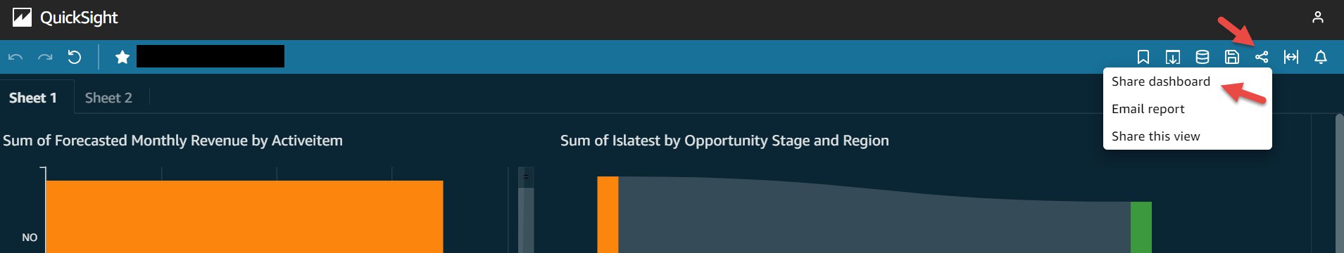
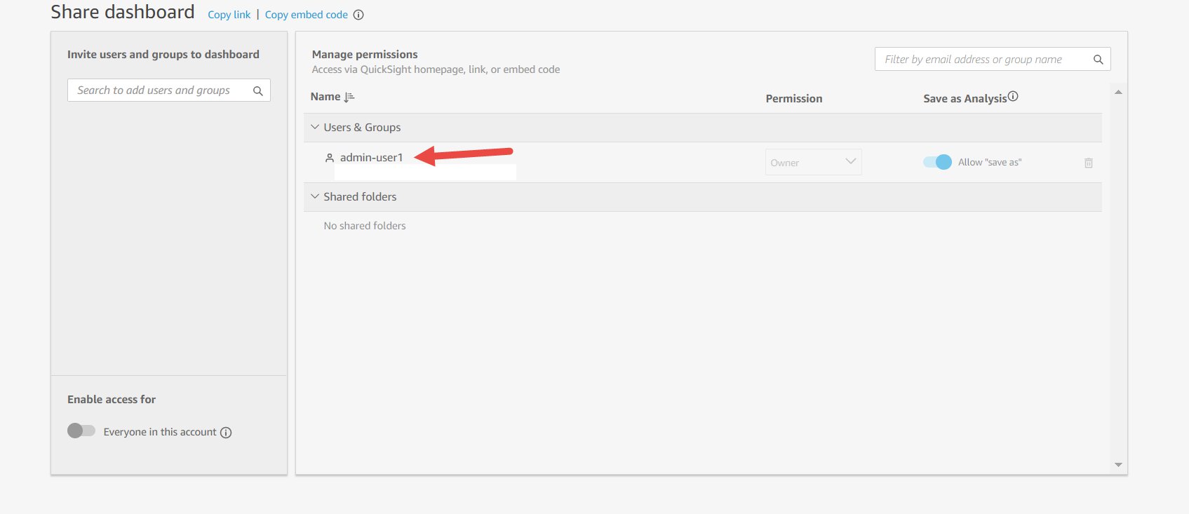
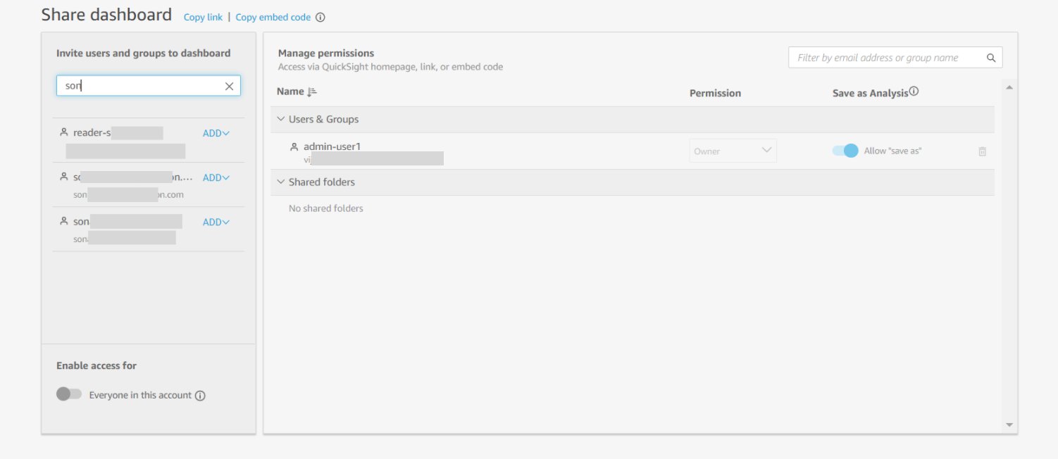
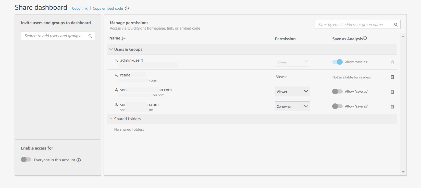
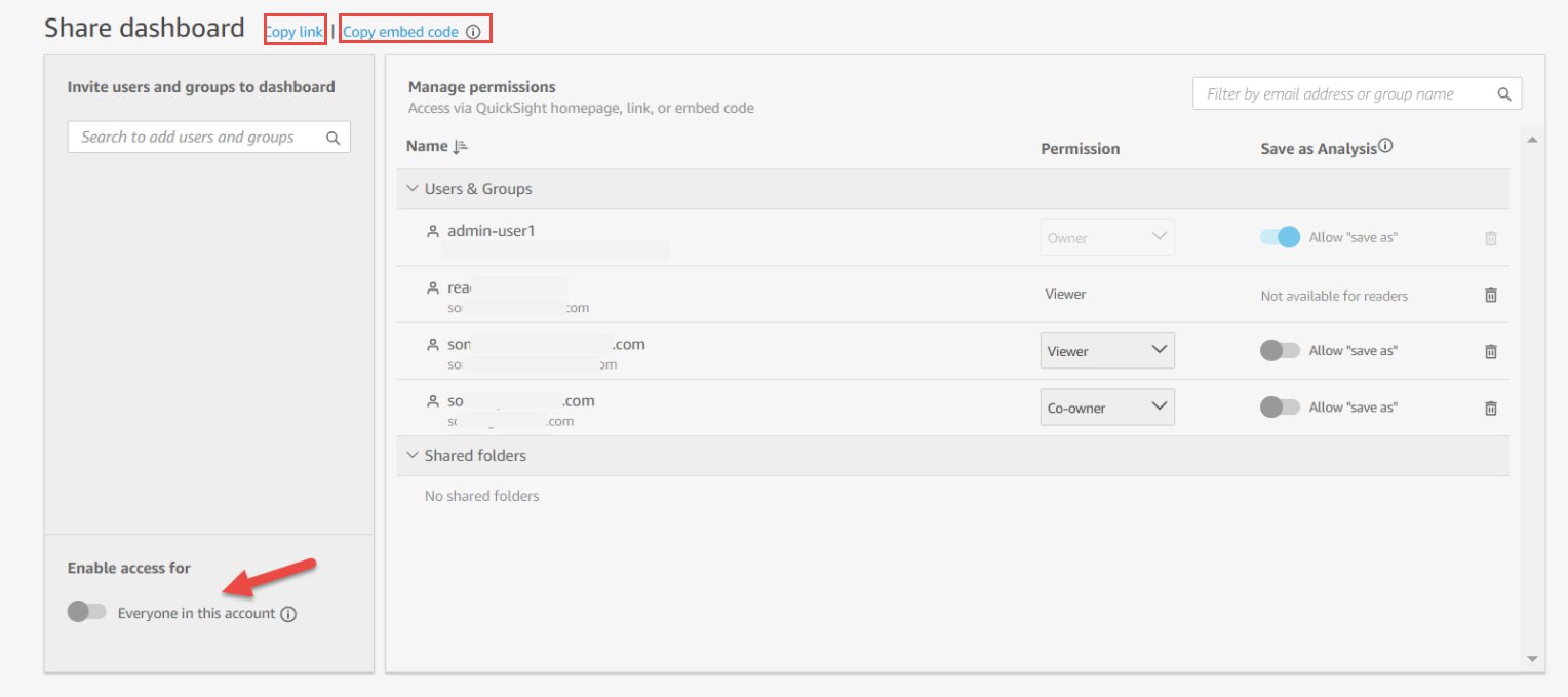
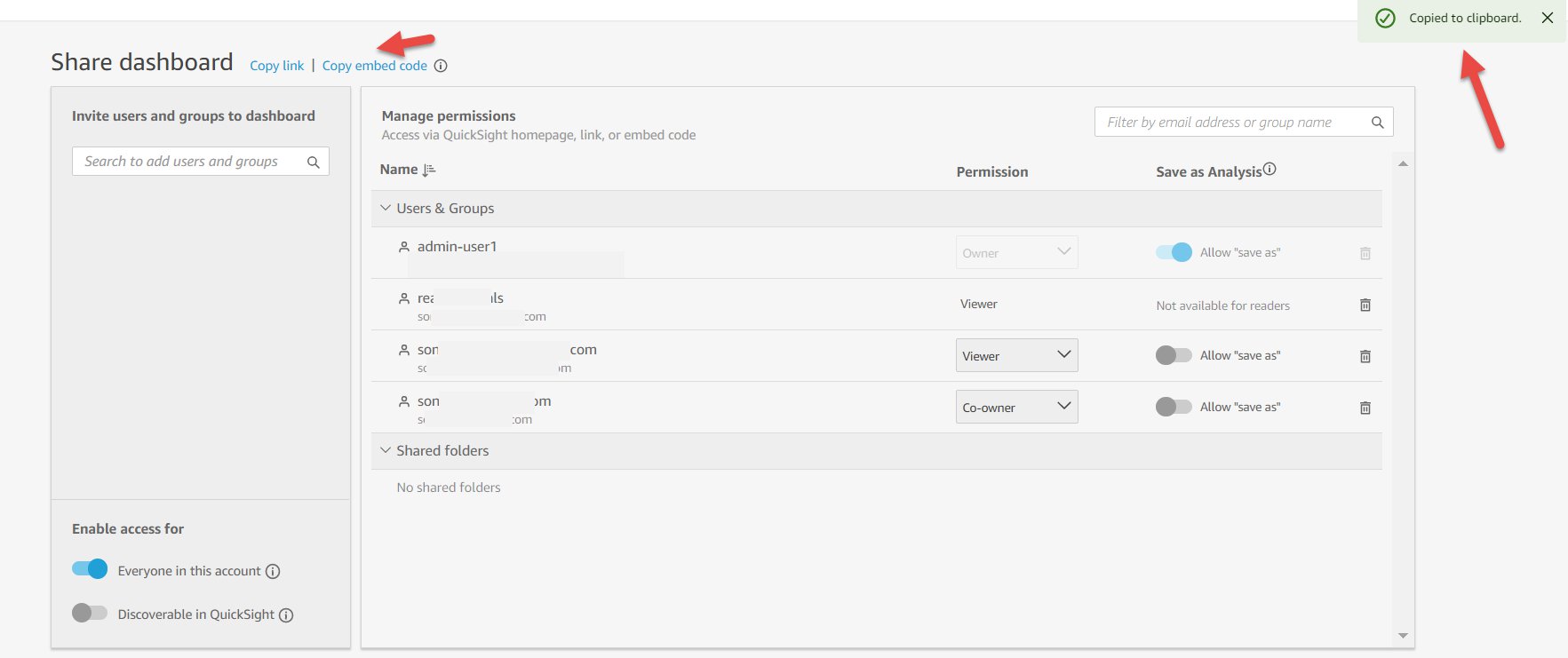
 To create a Quicksight dashboards from the Quicksight analysis click Share menu option at the top right corner then select publish dashboard”. Provide required dashboard name while publishing the dashboard”. Same dashboard can be shared with multiple audiences in the Organization.
 Following is the final version of the dashboard. As mentioned above Quicksight dashboards can be shared with other stakeholders and also complete dashboard can be exported as excel sheet.


 Kareem Syed-Mohammed is a Product Manager at Amazon QuickSight. He focuses on embedded analytics, APIs, and developer experience. Prior to QuickSight he has been with AWS Marketplace and Amazon retail as a PM. Kareem started his career as a developer and then PM for call center technologies, Local Expert and Ads for Expedia. He worked as a consultant with McKinsey and Company for a short while.
 Raji Sivasubramaniam is a Specialist Solutions Architect at AWS, focusing on Analytics. Raji has 20 years of experience in architecting end-to-end Enterprise Data Management, Business Intelligence and Analytics solutions for Fortune 500 and Fortune 100 companies across the globe. She has in-depth experience in integrated healthcare data and analytics with wide variety of healthcare datasets including managed market, physician targeting and patient analytics. In her spare time, Raji enjoys hiking, yoga and gardening.
 Srikanth Baheti is a Specialized World Wide Sr. Solution Architect for Amazon QuickSight. He started his career as a consultant and worked for multiple private and government organizations. Later he worked for PerkinElmer Health and Sciences & eResearch Technology Inc, where he was responsible for designing and developing high traffic web applications, highly scalable and maintainable data pipelines for reporting platforms using AWS services and Serverless computing.-