Post Syndicated from Karim Hammouda original https://aws.amazon.com/blogs/big-data/simplify-data-discovery-for-business-users-by-adding-data-descriptions-in-the-aws-glue-data-catalog/
In this post, we discuss how to use AWS Glue Data Catalog to simplify the process for adding data descriptions and allows data analysts to access, search, and discover this cataloged metadata with BI tools.
In this solution, we use AWS Glue Data Catalog, to break the silos between cross-functional data producer teams, sometimes also known as domain data experts, and business-focused consumer teams that author business intelligence (BI) reports and dashboards.
| Since you’re reading this post, you may also be interested in the following:
|
Data democratization and the need for self-service BI
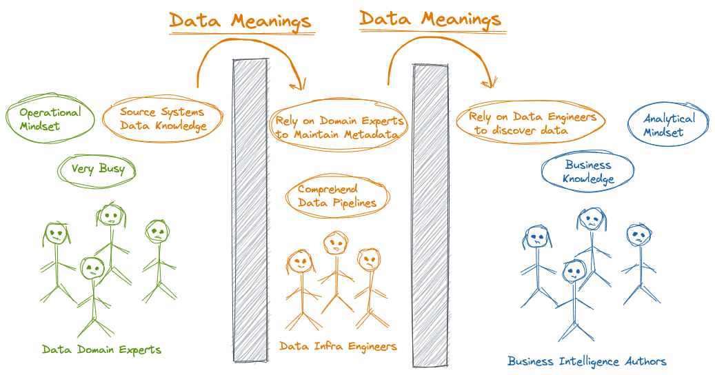
To be able to extract insights and get value out of organizational-wide data assets, data consumers like data analysts need to understand the meaning of existing data assets. They rely on data platform engineers to perform such data discovery tasks on their behalf.
Although data platform engineers can programmatically extract and obtain some technical and operational metadata, such as database and table names and sizes, column schemas, and keys, this metadata is primarily used for organizing and manipulating data inside the data lake. They still rely on source data domain experts to gain more knowledge about the meaning of the data, its business context, and classification. It becomes more challenging when data domain experts tend to prioritize operational-critical requests and delay the analytical-related ones.
Such a cycled dependency, as illustrated in the following figure, can delay the organizational strategic vision for implementing a self-service data analytics platform to reduce the time of the data-to-insights process.

Solution overview
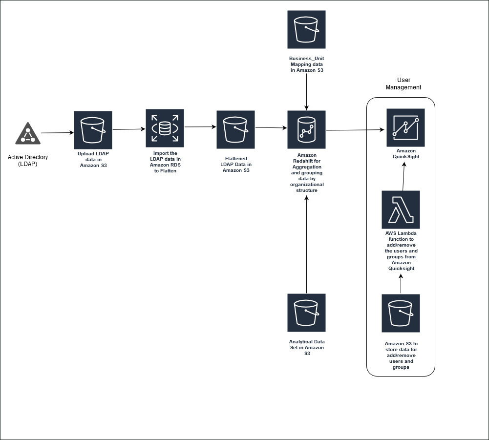
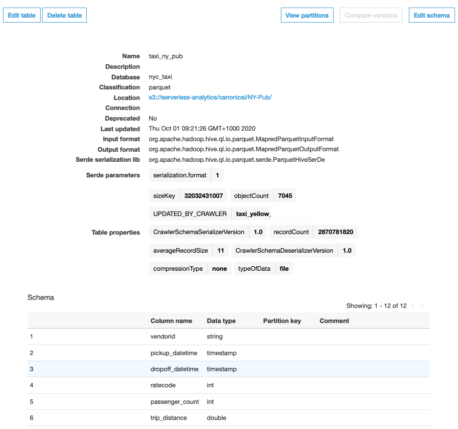
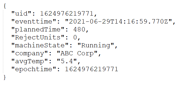
The Data Catalog fundamentally holds basic information about the actual data stored in various data sources, including but not limited to Amazon Simple Storage Service (Amazon S3), Amazon Relational Database Service (Amazon RDS), and Amazon Redshift. Information like data location, format, and columns schema can be automatically discovered and stored as tables, where each table specifies a single data store.
Throughout this post, we see how we can use the Data Catalog to make it easy for domain experts to add data descriptions, and for data analysts to access this metadata with BI tools.
First, we use the comment field in Data Catalog schema tables to store data descriptions with more business meaning. Comment fields aren’t like the other schema table fields (such as column name, data type, and partition key), which are typically populated automatically by an AWS Glue crawler.
We also use Amazon AI/ML capabilities to initially identify the description of each data entity. One way to do that is by using the Amazon Comprehend text analysis API. When we provide a sample of values for each data entity type, Amazon Comprehend natural language processing (NLP) models can identify a standard range of data classification, and we can use this as a description for identified data entities.
Next, because we need to identify entities unique to our domain or organization, we can use custom named entity recognition (NER) in Amazon Comprehend to add more metadata that is related to our business domain. One way to train custom NER models is to use Amazon SageMaker Ground Truth; for more information, see Developing NER models with Amazon SageMaker Ground Truth and Amazon Comprehend.
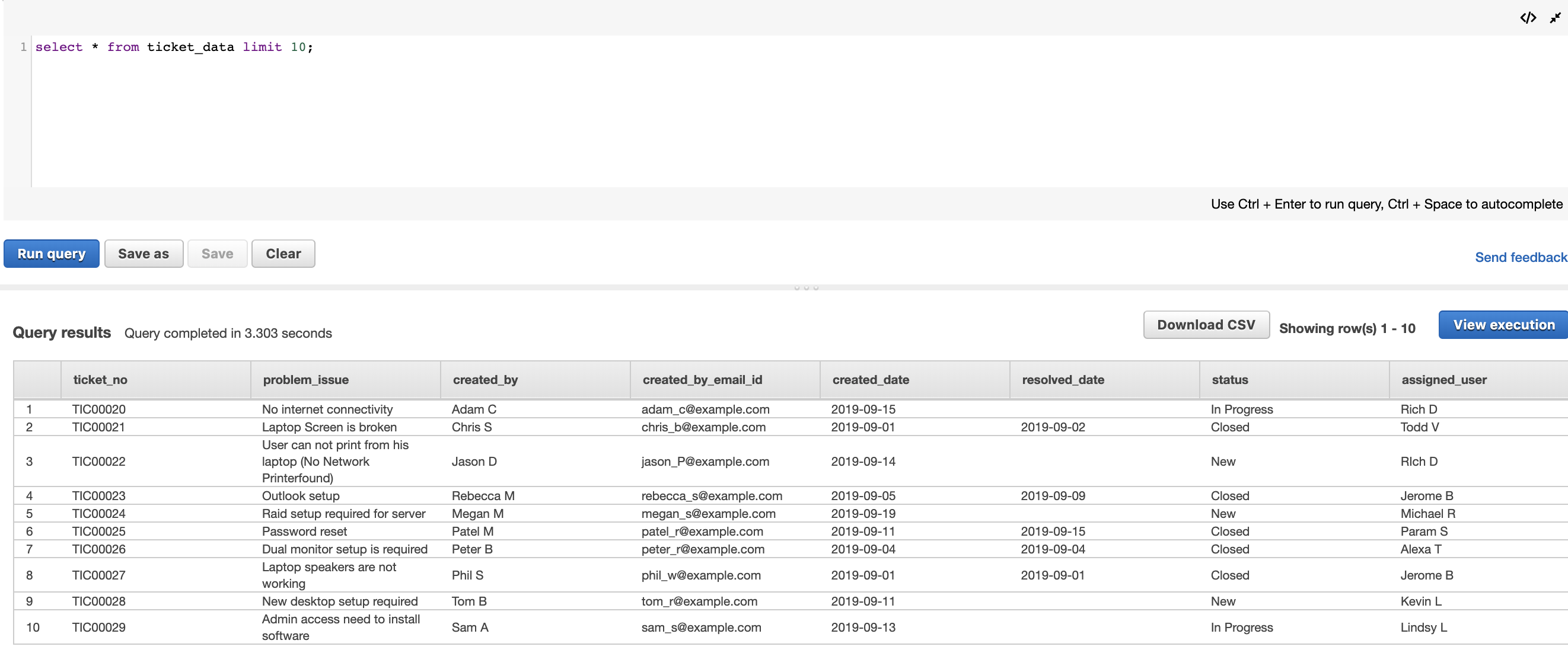
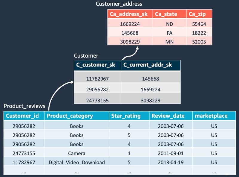
For this post, we use a dataset that has a table schema defined as per TPC-DS, and was generated using a data generator developed as part of AWS Analytics Reference Architecture code samples.
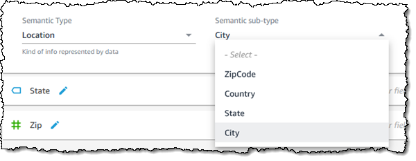
In this example, Amazon Comprehend API recognizes PII-related fields like Aid as a MAC address. While the none PII-related fields like Estatus, aren’t recognized. Therefore, the user enters a custom description manually, and we use the custom NER to automatically populate those fields, as shown in the following diagram.

After we add data meanings, we need to expose all the metadata captured in the Data Catalog to various data consumers. This can be done two different ways:
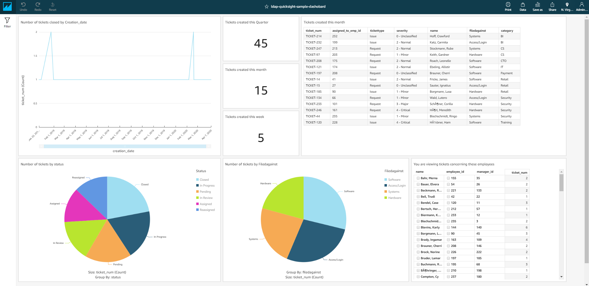
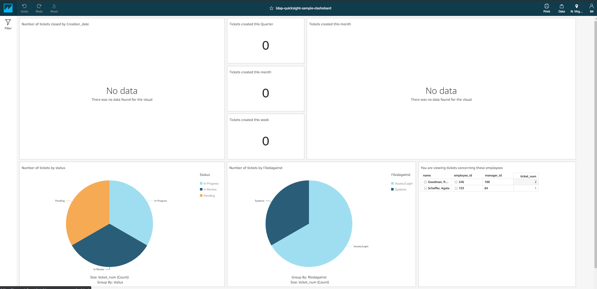
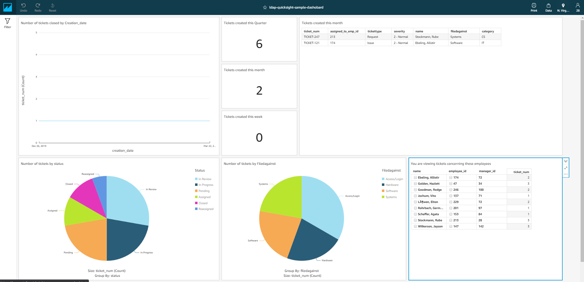
We can also use the latter method to expose the Data Catalog to BI authors comprehending data analyses and dashboards using Amazon QuickSight, so we use the second method for this post.
We do this by defining an Athena dataset that queries the information_schema and allows BI authors to use the QuickSight capability of text search filter to search and discover data using its business meaning (see the following diagram).

Solution details
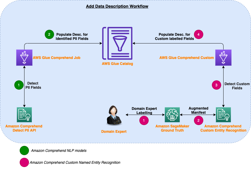
The core part of this solution is done using AWS Glue jobs. We use two AWS Glue jobs, which are responsible for calling Amazon Comprehend APIs and updating the AWS Glue Data Catalog with added data descriptions accordingly.
The first job (Glue_Comprehend_Job) performs the first stage of detection using the Amazon Comprehend Detect PII API, and the second job (Glue_Comprehend_Custom) uses Amazon Comprehend custom entity recognition for entities labeled by domain experts. The following diagram illustrates this workflow.

We describe the details of each stage in the upcoming sections.
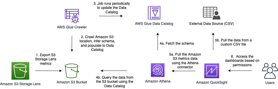
You can integrate this workflow into your existing data processing pipeline, which might be orchestrated with AWS services like AWS Step Functions, Amazon Managed Workflows for Apache Airflow (Amazon MWAA), AWS Glue workflows, or any third-party orchestrator.
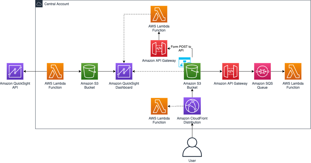
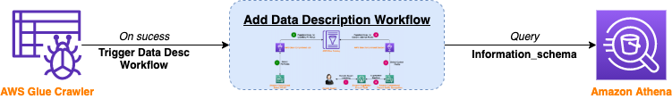
The workflow can complement AWS Glue crawler functionality and inherit the same logic for scheduling and running crawlers. On the other end, we can query the updated Data Catalog with data descriptions via Athena (see the following diagram).

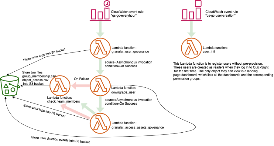
To show an end-to-end implementation of this solution, we have adopted a choreographically built architecture with additional AWS Lambda helper functions, which communicate between AWS services, triggering the AWS Glue crawler and AWS Glue jobs.
Stage-one: Enrich the Data Catalog with a standard built-in Amazon Comprehend entity detector
To get started, Choose  to launch a CloudFormation stack.
Define unique S3 bucket name and on the CloudFormation console, accept default values for the parameters.
This CloudFormation stack consists of the following:
- An AWS Identity Access Management (IAM) role called
Lambda-S3-Glue-comprehend.
- An S3 bucket with a bucket name that can be defined based on preference.
- A Lambda function called
trigger_data_cataloging. This function is automatically triggered when any CSV file is uploaded to the folder row_data inside our S3 bucket. Then it creates an AWS Glue database if one doesn’t exist, and creates and runs an AWS Glue crawler called glue_crawler_comprehend.
- An AWS Glue job called
Glue_Comprehend_Job, which calls Amazon Comprehend APIs and updates the AWS Glue Data Catalog table accordingly.
- A Lambda function called
Glue_comprehend_workflow, which is triggered when the AWS Glue Crawler successfully finishes and calls the AWS Glue job Glue_Comprehend_Job.
To test the solution, create a prefix called row_data under the S3 bucket created from the CF stack, then upload the customer dataset sample to the prefix.
The first Lambda function is triggered to run the subsequent AWS Glue crawler and AWS Glue job to get data descriptions using Amazon Comprehend, and it updates the comment section of the dataset created in the AWS Glue Data Catalog.

Stage-two: Use Amazon Comprehend custom entity recognition
Amazon Comprehend was able to detect some of the entity types within the customer sample dataset. However, for the remaining undetected fields, we can get help from a domain data expert to label a sample dataset using Ground Truth. Then we use the labeled data output to train a custom NER model and rerun the AWS Glue job to update the comment column with a customized data description.
Train an Amazon Comprehend custom entity recognition model
One way to train Amazon Comprehend custom entity recognizers is to get augmented manifest information using Ground Truth to label the data. Ground Truth has a built-in NER task for creating labeling jobs so domain experts can identify entities in text. To learn more about how to create the job, see Named Entity Recognition.
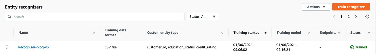
As an example, we tagged three labels entities: customer information ID, current level of education, and customer credit rating. The domain experts get a web interface like one shown in the following screenshot to label the dataset.

We can use the output of the labeling job to train an Amazon Comprehend custom entity recognition model using the augmented manifest.
The augmented manifest option requires a minimum of 1,000 custom entity recognition samples. Another option can be to use a CSV file that contains the annotations of the entity lists for the training dataset. The required format depends on the type of CSV file that we provide. In this post, we use the CSV entity lists option with two sample files:
To create the training job, we can use the Amazon Comprehend console, the AWS Command Line Interface (AWS CLI), or the Amazon Comprehend API. For this post, we use the API to programmatically create a training Lambda function using the AWS SDK for Python, as shown on GitHub.
The training process can take approximately 15 minutes. When the training process is complete, choose the recognizer and make a note of the recognizer ARN, which we use in the next step.

Run custom entity recognition inference
When the training job is complete, create an Amazon Comprehend analysis job using the console or APIs as shown on GitHub.
The process takes approximately 10 minutes, and again we need to make a note of the output job file.

Create an AWS Glue job to update the Data Catalog
Now that we have the Amazon Comprehend inference output, we can use the following AWS CLI command to create an AWS Glue job that updates the Data Catalog Comment fields for this dataset with customized data description.
Download the AWS Glue job script from the GitHub repo, upload to the S3 bucket created from the CF Stack in stage-1, and run the following AWS CLI command:
aws glue create-job
--name "Glue_Comprehend_Job_custom_entity"
--role "Lambda-S3-Glue-comprehend"
--command '{"Name" : "pythonshell", "ScriptLocation" : "s3://<Your S3 bucket>/glue_comprehend_workflow_custom.py","PythonVersion":"3"}'
--default-arguments '{"--extra-py-files": "s3://aws-bigdata-blog/artifacts/simplify-data-discovery-for-business-users/blog/python/library/boto3-1.17.70-py2.py3-none-any.whl" }'
After you create the AWS Glue job, edit the job script and update the bucket and key name variables with the output data location of the Amazon Comprehend analysis jobs and run the AWS Glue job. See the following code:
bucket ="<Bucket Name>"
key = "comprehend_output/<Random number>output/output.tar.gz"
When the job is complete, it updates the Data Catalog with customized data descriptions.

Expose Data Catalog data to data consumers for search and discovery
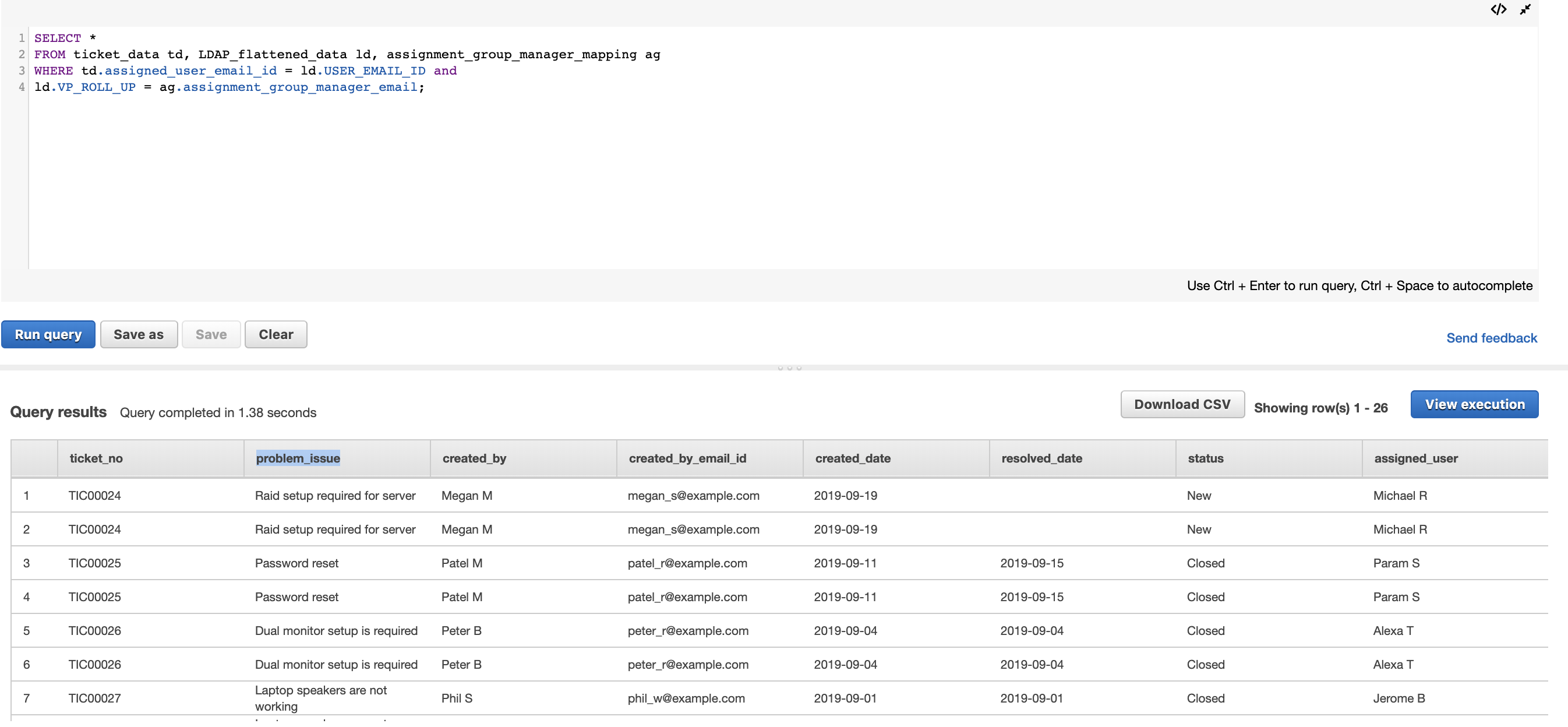
Data consumers that prefer using SQL can use Athena to run queries against the information_schema.columns table, which includes the comment field of the Data Catalog. See the following code:
SELECT table_catalog,
         table_schema,
         table_name,
         column_name,
         data_type,
         comment
FROM information_schema.columns
WHERE comment LIKE '%customer%'
AND table_name = 'row_data_row_data'
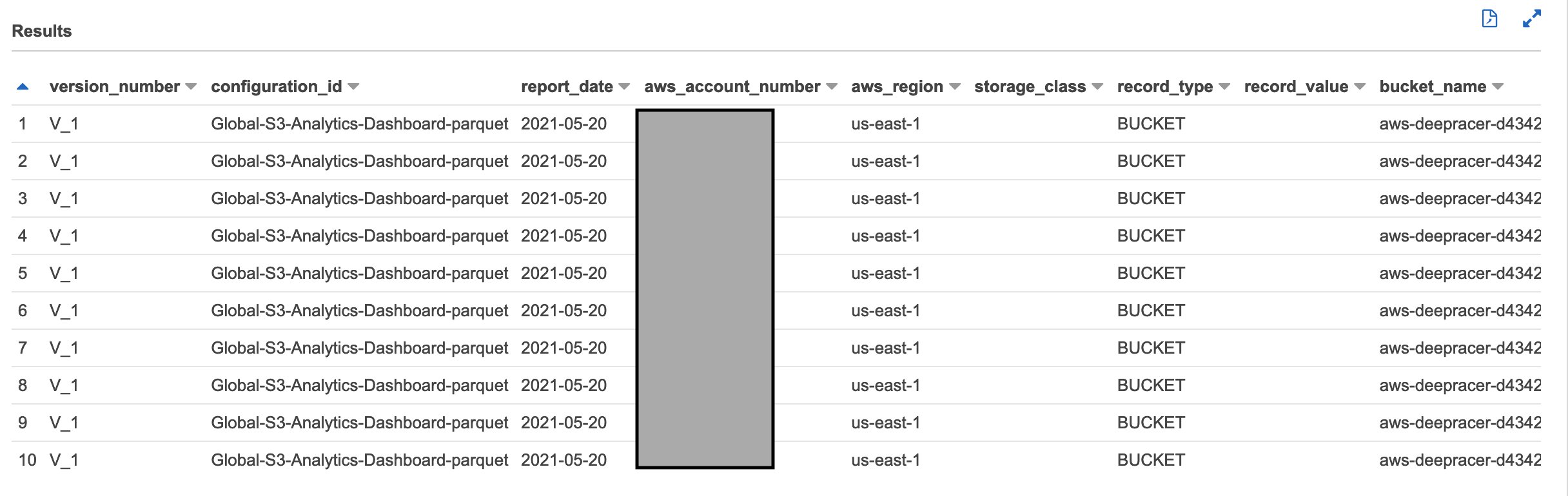
The following screenshot shows our query results.

The query searches all schema columns that might have any data meanings that contain customer; it returns crating, which contains customer in the comment field.
BI authors can use text search instead of SQL to search for data meanings of data stored in an S3 data lake. This can be done by setting up a visual layer on top of Athena inside QuickSight.
QuickSight is scalable, serverless, embeddable, and machine learning (ML) powered BI tool that is deeply integrated with other AWS services.
BI development in QuickSight is organized as a stack of datasets, analyses, and dashboards. We start by defining a dataset from a list of various integrated data sources. On top of this dataset, we can design multiple analyses to uncover hidden insights and trends in the dataset. Finally, we can publish these analyses as dashboards, which is the consumable form that can be shared and viewed across different business lines and stakeholders.
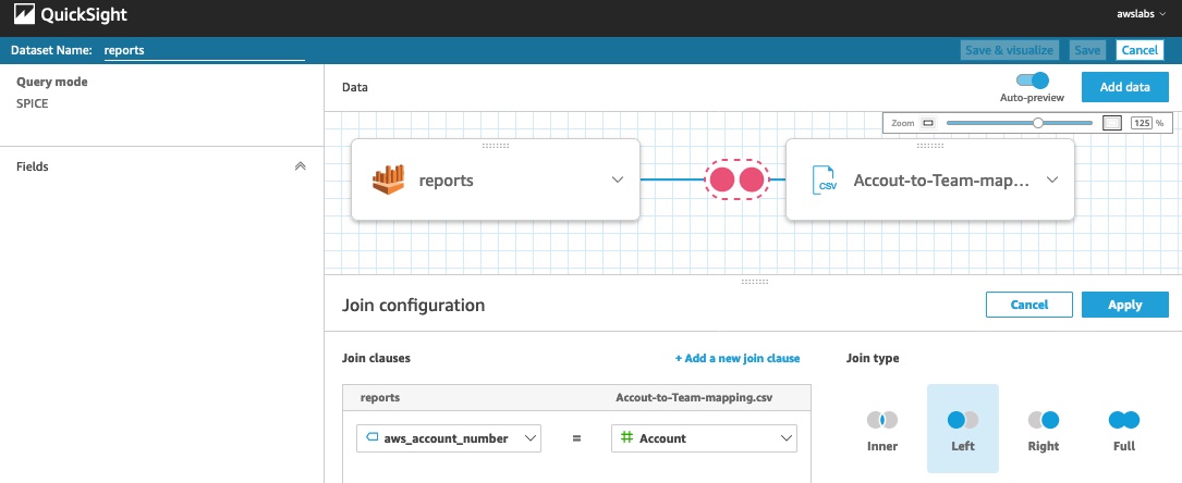
We want to help the BI authors while designing analyses to get a better knowledge of the datasets they’re working on. To do so, we first need to connect to the data source where the metadata is stored, in this case the Athena table information_schema.columns, so we create a dataset to act as a Data Catalog view inside QuickSight.
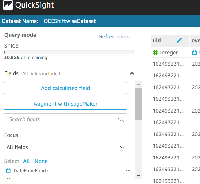
QuickSight offers different modes of querying data sources, which is decided as part of the dataset creation process. The first mode is called direct query, in which the fetching query runs directly against the external data source. The second mode is a caching layer called QuickSight Super-fast Parallel In-memory Calculation Engine (SPICE), which improves performance when data is shared and retrieved by various BI authors. In this mode, the data is stored locally and can be reused multiple times, instead of running queries against the data source every time the data needs to be retrieved. However, as with all caching solutions, you must take data volume limits into consideration while choosing datasets to be stored in SPICE.
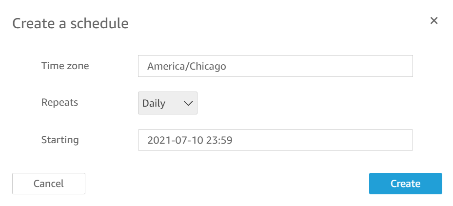
In our case, we choose to keep the Data Catalog dataset in SPICE, because the volume of the dataset is relatively small and won’t consume a lot of SPICE resources. However, we need to decide if we want to refresh the data cached in SPICE. The answer depends on how frequently the data schema and Data Catalog change, but in any case we can use the built-in scheduling within QuickSight to refresh SPICE at the desired interval. For information about triggering a refresh in an event-based manner, see Event-driven refresh of SPICE datasets in Amazon QuickSight.
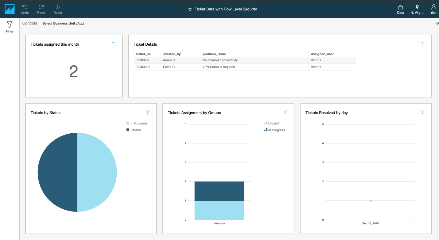
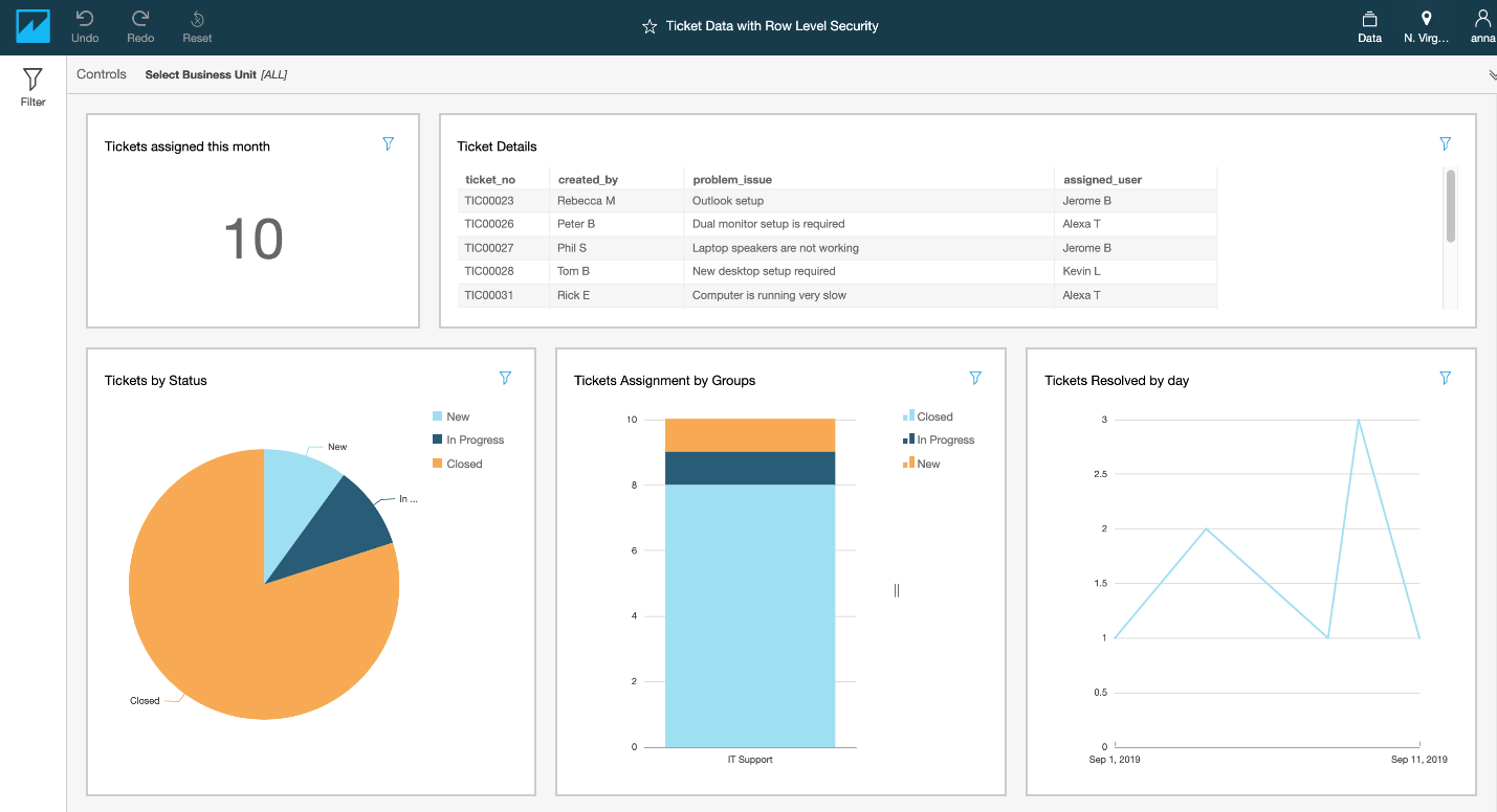
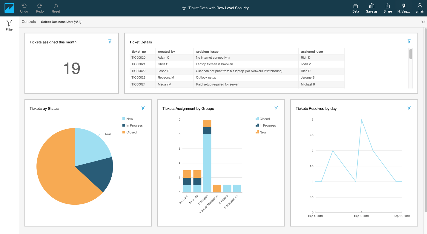
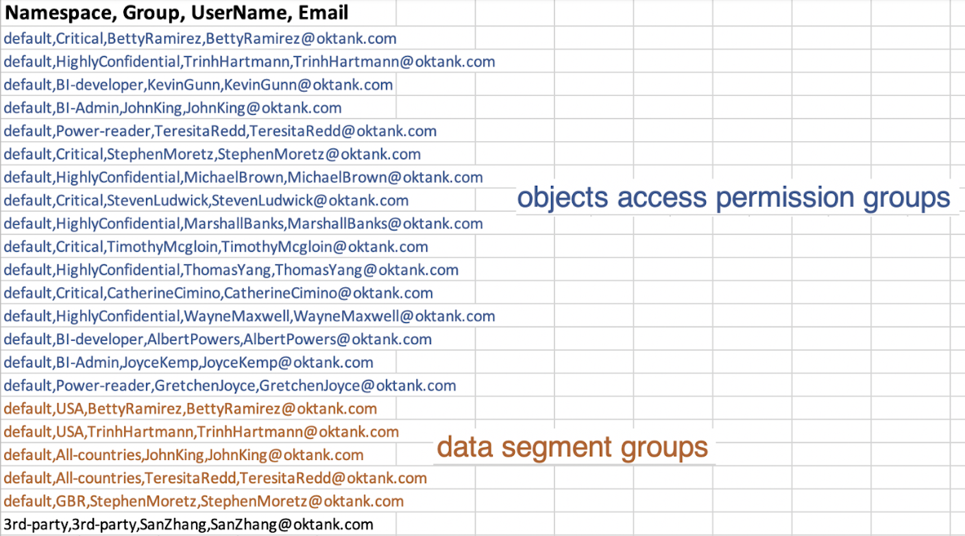
After we create the Data Catalog view as a dataset inside QuickSight stored in SPICE, we can use row-level security to restrict the access to this dataset. Each BI author has access with respect to their privileges for columns they can view metadata for.
Next, we see how we can allow BI authors to search through data descriptions populated in the comment field of the Data Catalog dataset. QuickSight offers features like filters, parameters, and controls to add more flexibility into QuickSight analyses and dashboards.
Finally, we use the QuickSight capability to add more than one dataset within an analysis view to allow BI authors to switch between the metadata for the dataset and the actual dataset. This allows the BI authors to self-serve, reducing dependency on data platform engineers to decide which columns they should use in their analyses.
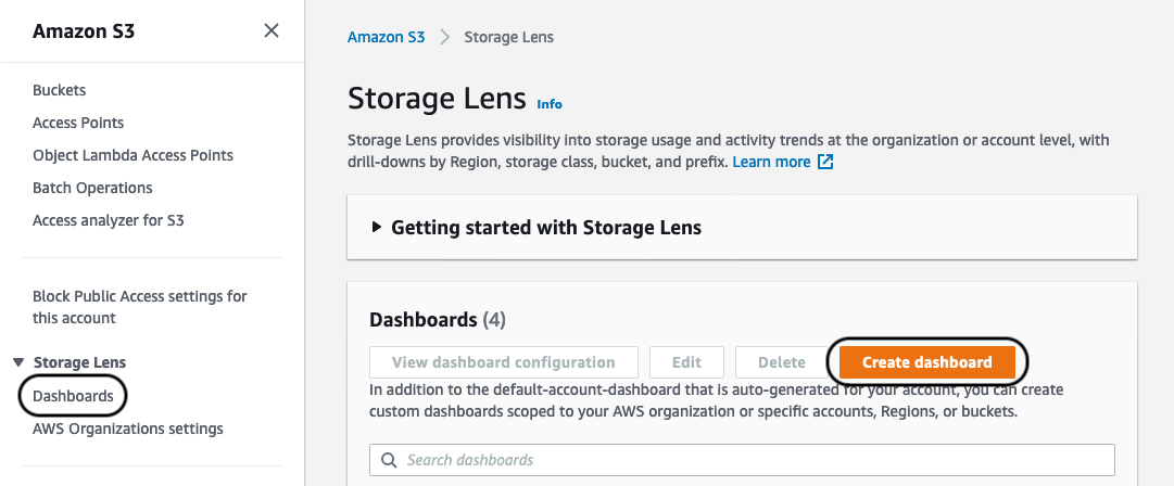
To set up a simple Data Catalog search and discovery inside QuickSight, complete the following steps:
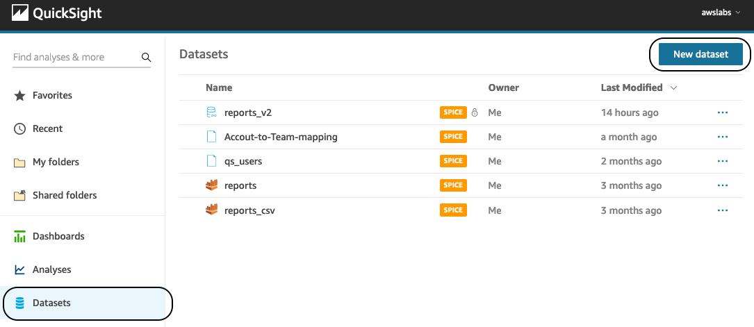
- On the QuickSight console, choose Datasets in the navigation pane.
- Choose New dataset.
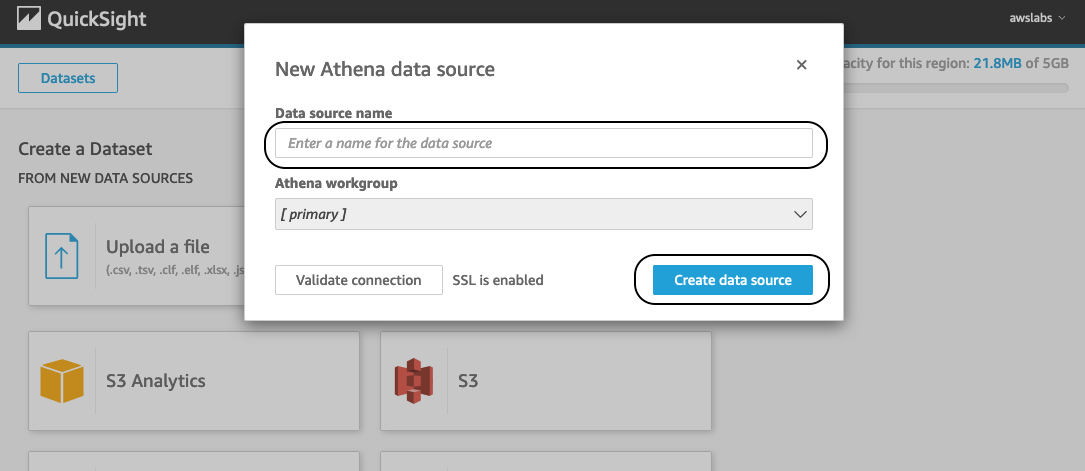
- For New data sources, choose Amazon Athena.
- Name the dataset
Data Catalog.
- Choose Create data source.
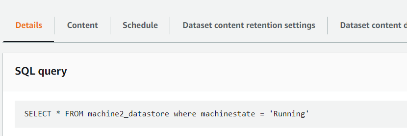
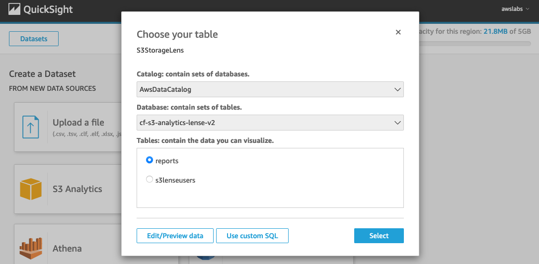
- For Choose your table, choose Use custom SQL.
- For Enter custom SQL query, name the query
Data Catalog Query.
- Enter the following query:
SELECT * FROM information_schema.columns
- Choose Confirm query.
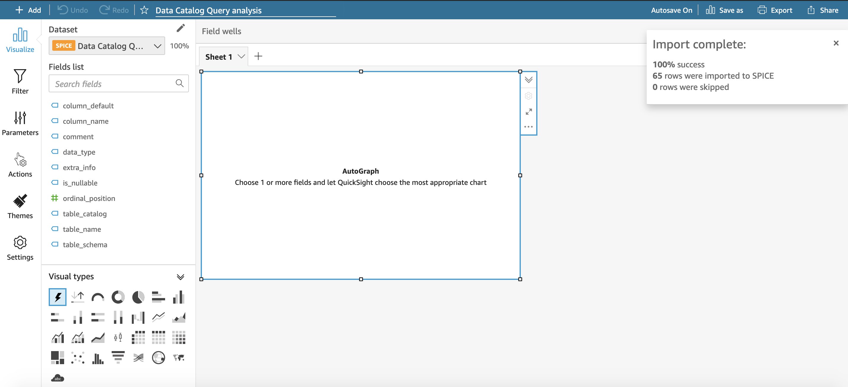
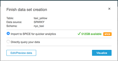
- Select Import to QuickSight SPICE for quicker analytics.
- Choose Visualize.

Next, we design an analysis on the dataset we just created to access the Data Catalog through Athena.
When we choose Visualize, we’re redirected to the QuickSight workspace to start designing our analysis.

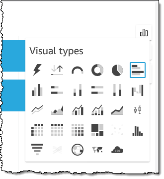
- Under Visual types, choose Table.
- Under Fields list, add
table_name, column_name, and comment to the Values field well.

Next, we use the filter control feature to allow users to perform text search for data descriptions.
- In the navigation pane, choose Filter.
- Choose the plus sign (+) to access the Create a new filter list.
- On the list of columns, choose
comment to be the filter column.
- From the options menu (…) on the filter, choose Add to sheet.
We should be able to see a new control being added into our analysis to allow users to search the comment field.
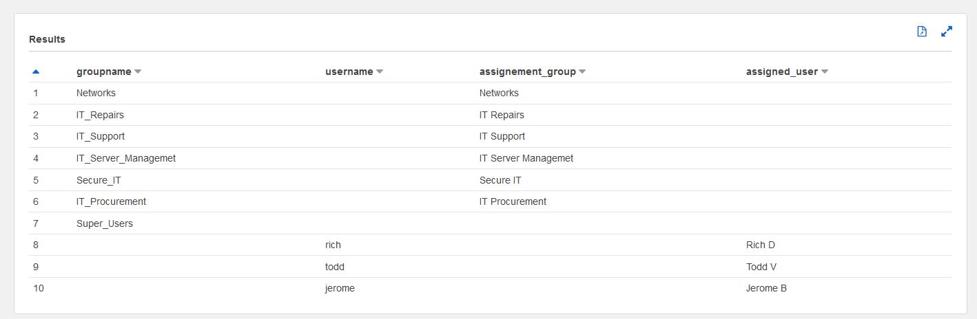
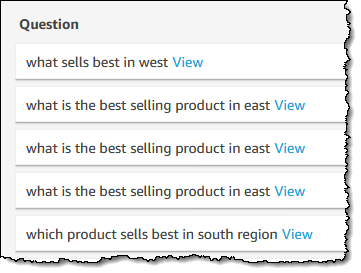
Now we can start a text search for data descriptions that contain customer, where QuickSight shows the list of fields matching the search criteria and provides table and column names accordingly.

Alternatively, we can use parameters to be associated with the filter control if needed, for example to connect one dashboard to another. For more information, see the GitHub repo.
Finally, BI authors can switch between the metadata view that we just created and the actual Athena table view (row_all_row_data), assuming it’s already imported (if not, we can use the same steps from earlier to import the new dataset).
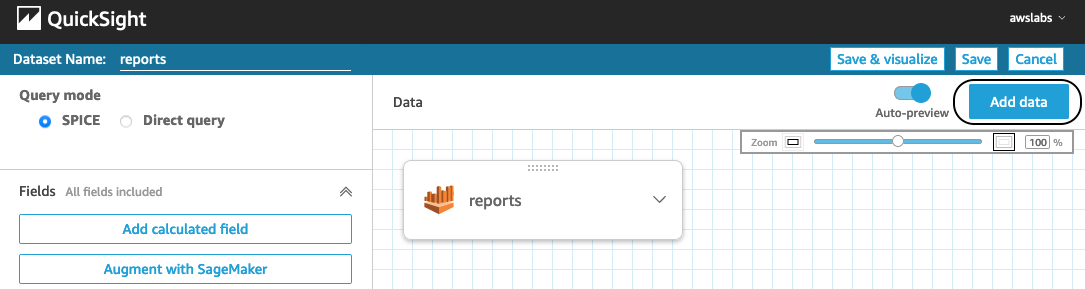
- In the navigation pane, choose Visualize.
- Choose the pen icon to add, edit, replace, or remove datasets.
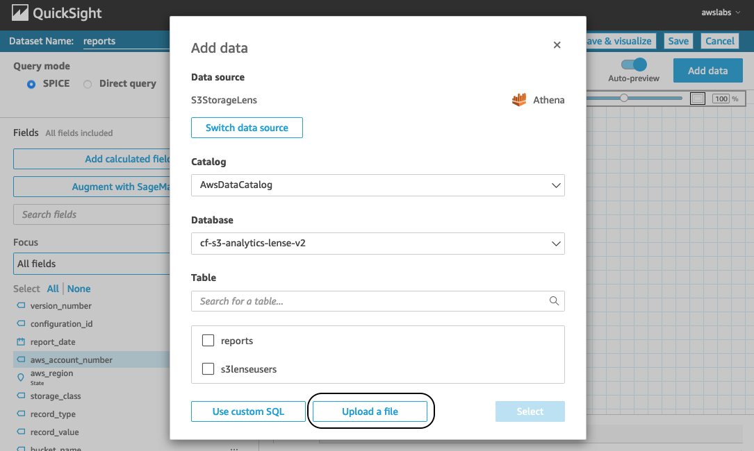
- Choose Add dataset.
- Add
row_all_row_data.
- Choose Select.
BI authors can now switch between data and metadata datasets.

They now have a metadata view along with the actual data view, so they can better understand the meaning of each column in the dataset they’re working on, and they can read any comment that can be passed from other teams within the organization without needing to do this manually.
Conclusion
In this post, we showed how to build a quick workflow using AWS Glue and Amazon AI/ML services to complement the AWS Glue crawler functionality. You can integrate this workflow into a typical AWS Glue data cataloging and processing pipeline to achieve alignment between cross-functional teams by simplifying and automating the process of adding data descriptions in the Data Catalog. This is an important step in data discovery, and the topic will be covered more in upcoming posts.
This solution is also a step towards implementing data privacy and protection regimes such as the Health Insurance Portability and Accountability Act (HIPAA) and General Data Protection Regulation (GDPR) by identifying sensitive data types like PII and enforcing access polices.
You can find the source code from this post on GitHub and use it to build your own solution. For more information about NER models, see Developing NER models with Amazon SageMaker Ground Truth and Amazon Comprehend.
About the Authors
 Karim Hammouda is a Specialist Solutions Architect for Analytics at AWS with a passion for data integration, data analysis, and BI. He works with AWS customers to design and build analytics solutions that contribute to their business growth. In his free time, he likes to watch TV documentaries and play video games with his son.
 Ahmed Raafat is a Senior Solutions Architect at Amazon Web Services, with a passion for machine learning solutions. Ahmed acts as a trusted advisor for many AWS enterprise customers to support and accelerate their cloud journey.


 Lotfi is a Senior Solutions Architect working for the Public Sector team with Amazon Web Services. He helps public sector customers across EMEA realize their ideas, build new services, and innovate for citizens. In his spare time, Lotfi enjoys cycling and running.


 Lotfi Mouhib is a Senior Solutions Architect working for the Public Sector team with Amazon Web Services. He helps public sector customers across EMEA realize their ideas, build new services, and innovate for citizens. In his spare time, Lotfi enjoys cycling and running.


 To recap, Q is a natural language query tool for the Enterprise Edition of


 Kareem Syed-Mohammed is a Product Manager at Amazon QuickSight. He focuses on embedded analytics, APIs, and developer experience. Prior to QuickSight he has been with AWS Marketplace and Amazon retail as a PM. Kareem started his career as a developer and then PM for call center technologies, Local Expert and Ads for Expedia. He worked as a consultant with McKinsey and Company for a short while.


 Jignesh Gohel is a Technical Account Manager at AWS. In this role, he provides advocacy and strategic technical guidance to help plan and build solutions using best practices, and proactively keep customers’ AWS environments operationally healthy. He is passionate about building modular and scalable enterprise systems on AWS using serverless technologies. Besides work, Jignesh enjoys spending time with family and friends, traveling and exploring the latest technology trends.
 Suman Koduri is a Global Category Lead for Data & Analytics category in AWS Marketplace. He is focused towards business development activities to further expand the presence and success of Data & Analytics ISVs in AWS Marketplace. In this role, he leads the scaling, and evolution of new and existing ISVs, as well as field enablement and strategic customer advisement for the same. In his spare time, he loves running half marathon’s and riding his motorcycle.