Tag Archives: AWS re:Invent

Preview: Amazon OpenSearch Serverless – Run Search and Analytics Workloads without Managing Clusters

Post Syndicated from Channy Yun original https://aws.amazon.com/blogs/aws/preview-amazon-opensearch-serverless-run-search-and-analytics-workloads-without-managing-clusters/

Most AWS analytics services have compelling serverless offerings that make it even easier for customers to analyze vast amounts of data without having to configure, scale, or manage the underlying infrastructure.

Along with other serverless analytics, such as Amazon QuickSight for business intelligence and AWS Glue for data integration, we have introduced Amazon EMR Serverless, Amazon MSK Serverless, and Amazon Redshift Serverless this year.

Today, we announce the preview release of a new serverless option for Amazon OpenSearch Service that makes it easy for customers to run large-scale search and analytics workloads without managing clusters. It automatically provisions and scales the underlying resources to deliver fast data ingestion and query responses for even the most demanding and unpredictable workloads, eliminating the need to configure and optimize clusters.

With Amazon OpenSearch Serverless, you do not need to account for factors that are hard to know in advance, such as the frequency and complexity of queries or the volume of data expected to be analyzed. Instead of managing infrastructure, you can focus on using OpenSearch for exploring and deriving insights from your data. You can also get started using familiar APIs to load and query data and use OpenSearch Dashboards for interactive data analysis and visualization.

Configure Your OpenSearch Serverless Collection
To get started with Amazon OpenSearch Serverless, you create a Collection via the AWS Management Console, AWS Command-Line Interface (AWS CLI), or AWS API.

Before the launch of OpenSearch Serverless, you created a managed cluster, specifying instance types, counts, and storage options, and then managed the lifecycle and shard strategy for indices within that cluster. With OpenSearch Serverless, you create a Collection, which manages a group of indices that work together to support a specific workload. You no longer need to specify the hardware or manage the indices directly.

To create an OpenSearch Serverless collection and secure data, set up Encryption policies to assign AWS KMS keys to one or more collections and attach Network policies to collections to control the access from specified VPCs and public IP addresses.

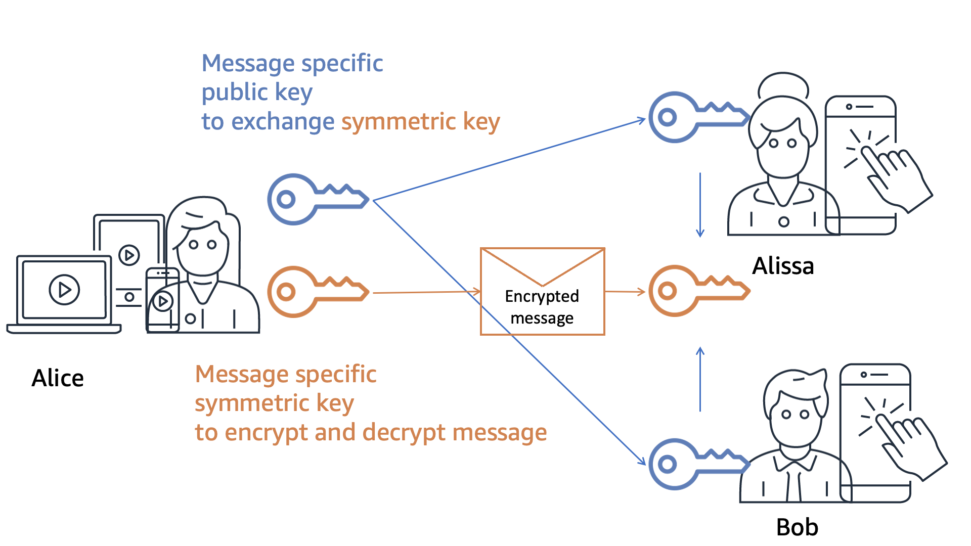
To create an encryption policy, choose Encryption policies in the left navigation pane and Create encryption policy. Encryption at rest secures the indices within your collection. For each collection, AWS KMS generates a unique, symmetric encryption key. Encryption policies are the optimal way to manage AWS KMS keys across multiple collections. You can define the target collection name or a prefix that automatically applies the encryption settings from this policy to the collection.

In order for users to access a collection, choose Network policies in the left navigation pane and Create network policy. Network policies determine whether your collection is accessible over the internet from public networks or whether it must be accessed through OpenSearch Serverless–managed VPC endpoints.

You can define multiple rules for each collection, either the Public or VPC, as a recommended option for the Access Type. If you select a public option, you can access the collection from OpenSearch Dashboards.

Also, you can configure access for OpenSearch Dashboards and the OpenSearch endpoint. For the Resource type, enable both Access to OpenSearch endpoints and Access to OpenSearch Dashboards. In both input boxes, select the Collection Name property and your collection name or prefix.

Finally, to create an OpenSearch Serverless collection, choose Create collection in the home page or choose Collections in the left navigation pane and choose Create collection.

Input your collection name, description, and collection type, either Time series or Search by your data type.

  • Time series – The log analytics segment that focuses on analyzing large volumes of semistructured, machine-generated data in real time for operational, security, user behavior, and business insights.
  • Search – Full-text search that powers applications in your internal networks (content management systems, legal documents) and internet-facing applications such as e-commerce website search and content search.

When you choose Create, a collection typically takes less than a minute to initialize.

Upload and Search Data in Your Collection
Before uploading and searching data in your collection, configure the IAM policy to access the actual data within a collection. Choose Data access policies in the left navigation pane and Create data access policy.

You can apply multiple policies simultaneously to the same resource. Each policy contains a set of rules. Each rule has a resource (collection or index), permissions for the resource, and a list of principals (IAM users, role ARNs, or SAML identities).

Here is a sample policy that provides a single user the minimum permissions required to create an index in your collection, index some data, and search for it. Replace the principal ARN with the ARN of the account that you’ll use to sign in to OpenSearch Dashboards.

[
  {
    "Rules": [
      {
        "ResourceType": "index",
        "Resource": [
          "index/books/*"
        ],
        "Permission": [
          "aoss:CreateIndex",
          "aoss:ReadDocument",
          "aoss:UpdateIndex",
          "aoss:DeleteIndex",
          "aoss:WriteDocument"
        ]
      }
    ],
    "Principal": [
      "arn:aws:iam::123456789012:user/admin"
    ]
  }
]

Now, you can upload data to an OpenSearch Serverless collection using Postman or curl. You can also use Dev Tools within the OpenSearch Dashboards console. Choose OpenSearch Dashboards on the detail page of your collection.

Sign in to OpenSearch Dashboards using the AWS access and secret keys for the principal that you specified in your data access policy. Within OpenSearch Dashboards, open the left navigation menu and choose Dev Tools.

To create a single index called books-index, run PUT books-index, and index your first single document into books-index.

You can also query search data in Dev Tools.

GET books_index/_search
{
    "query": {
    "simple_query_string": {
    "query": "Jeff",
    "fields": ["author"]
    } 
  }
}

In the case of time-series data, you can ingest data with all of the streaming ingestion options, such as native OpenSearch streaming APIs, Amazon Kinesis Data Firehose, AWS Glue, and a wide range of open-source streaming ingestion pipelines like Logstash, FluentBit, Fluentd, and Data Prepper.

In addition, you can snapshot your data from a managed cluster on OpenSearch Service and restore it to your collection, making it easy to migrate your workloads. Once your data is in your collection, you can then query it using your favorite OpenSearch client and interactively analyze and visualize your data using OpenSearch Dashboards.

Things to Know
Here are a couple of things to keep in mind about additional features and considerations when you choose Amazon OpenSearch Serverless:

  • SAML Authentications – You can use your existing identity provider to offer single sign-on (SSO) for the OpenSearch Dashboards endpoints of OpenSearch Serverless SAML authentication lets you use third-party identity providers to sign in to OpenSearch Dashboards to index and search data. OpenSearch Serverless supports providers that use the SAML 2.0 standard, such as Okta, Keycloak, Active Directory Federation Services, and Auth0.
  • Private VPC Endpoints – You can use AWS PrivateLink to create a private connection between your VPC and OpenSearch Serverless. You can access your collections as if they were in your VPC without the use of an internet gateway, NAT device, VPN connection, or AWS Direct Connect connection. To create an interface endpoint, choose VPC endpoints in the left navigation pane of OpenSearch Service.
  • Managed Clusters – You may prefer to use an option of Amazon OpenSearch Service’s managed clusters in scenarios where you need tight control over cluster configuration or specific customizations. For example, your workloads may need custom plugins that run best on accelerated computing instances and need more control on configuration such as data sharding strategy. You can choose either provisioned instances or serverless according to the requirements of your workload.

Join the Preview
The preview release of Amazon OpenSearch Serverless is now available in the US East (N. Virginia, Ohio), US West (Oregon), EU (Ireland), Asia Pacific (Tokyo). With OpenSearch Serverless, there are no upfront costs, and you pay only for the data that is ingest and the queries you run. For pricing details, see the OpenSearch Service pricing page. To learn more, visit the Amazon OpenSearch Service User Guide.

We want to hear more feedback during the preview. Please send feedback to AWS re:Post for Amazon OpenSearch Service or through your usual AWS support contacts.

Channy

New – Accelerate Your Lambda Functions with Lambda SnapStart

Post Syndicated from Jeff Barr original https://aws.amazon.com/blogs/aws/new-accelerate-your-lambda-functions-with-lambda-snapstart/

Our customers tell me that they love AWS Lambda for many reasons. On the development side they appreciate the simple programming model and ease with which their functions can make use of other AWS services. On the operations side they benefit from the ability to build powerful applications that can respond quickly to changing usage patterns.

As you might know if you are already using Lambda, your functions are run inside of a secure and isolated execution environment. The lifecycle of each environment consists of three main phases: Init, Invoke, and Shutdown. Among other things, the Init phase bootstraps the runtime for the function and runs the function’s static code. In many cases, these operations are completed within milliseconds and do not lengthen the phase in any appreciable way. In the remaining cases, they can take a considerable amount of time, for several reasons. First, initializing the runtime for some languages can be expensive. For example, the Init phase for a Lambda function that uses one of the Java runtimes in conjunction with a framework such as Spring Boot, Quarkus, or Micronaut can sometimes take as long as ten seconds (this includes dependency injection, compilation of the code for the function, and classpath component scanning). Second, the static code might download some machine learning models, pre-compute some reference data, or establish network connections to other AWS services.

Introducing Lambda SnapStart
In order to allow you to put Lambda to use in even more ways, we are introducing Lambda SnapStart today.

After you enable Lambda SnapStart for a particular Lambda function, publishing a new version of the function will trigger an optimization process. The process launches your function and runs it through the entire Init phase. Then it takes an immutable, encrypted snapshot of the memory and disk state, and caches it for reuse. When the function is subsequently invoked, the state is retrieved from the cache in chunks on an as-needed basis and used to populate the execution environment. This optimization makes invocation time faster and more predictable, since creating a fresh execution environment no longer requires a dedicated Init phase.

We are launching with support for Java functions that make use of the Corretto (java11) runtime, and expect to see Lambda SnapStart put to use right away for applications that make use of Spring Boot, Quarkus, Micronaut, and other Java frameworks. Enabling Lambda SnapStart for Java functions can make them start up to 10x faster, at no extra cost.

Using Lambda SnapStart
Because my last actual encounter with Java took place in the last century, I used the Serverless Spring Boot 2 example from the AWS Labs repo as a starting point. I installed the AWS SAM CLI and did a test build & deploy to establish a baseline. I invoked the function and saw that the Init duration was slightly more than 6 seconds:

Then I added two lines to template.yml to configure the SnapStart property:

I rebuilt and redeployed, published a fresh version of the function to set up SnapStart, and ran another test:

With SnapStart, the initialization phase (represented by the Init duration that I showed you earlier) happens when I publish a new version of the function. When I invoke a function that has SnapStart enabled, Lambda restores the snapshot (represented by the Restore duration) before invoking the function handler. As a result, the total cold invoke with SnapStart is now Restore duration + Duration. SnapStart has reduced the cold start duration from over 6 seconds to less than 200 ms.

Becoming Snap-Resilient
Lambda SnapStart speeds up applications by reusing a single initialized snapshot to resume multiple execution environments. This has a few interesting implications for your code:

Uniqueness – When using SnapStart, any unique content that used to be generated during the initialization must now be generated after initialization in order to maintain uniqueness. If you (or a library that you reference) uses a pseudo-random number generator, it should not be based on a seed that is obtained during the Init phase. We have updated OpenSSL’s RAND_Bytes to ensure randomness when used in conjunction with SnapStart, and we have verified that java.security.SecureRandom is already snap-resilient. Amazon Linux’s /dev/random and /dev/urandom are also snap-resilient.

Network Connections -If your code creates long-term connections to network services during the Init phase and uses them during the Invoke phase, make sure that it can re-establish the connection if necessary. The AWS SDKs have already been updated to do this.

Ephemeral Data – This is effectively a more general form of the above items. If your code downloads or computes reference information during the Init phase, consider doing a quick check to make sure that it has not gone stale during the caching period.

Lambda provides a pair of runtime hooks to help you to maintain uniqueness, as well as a scanning tool to help detect possible issues.

Things to Know
Here are a couple of other things to know about Lambda SnapStart:

Caching – Cached snapshots are removed after 14 days of inactivity. Lambda will automatically refresh the cache if a snapshot depends on a runtime that has been updated or patched.

Pricing – There is no extra charge for the use of Lambda SnapStart.

Feature Compatibility – You cannot use Lambda SnapStart with larger ephemeral storage, Elastic File Systems, Provisioned Concurrency, or Graviton2. In general, we recommend using SnapStart for your general-purpose Lambda functions and Provisioned Concurrency for the subset of those functions that are exceptionally sensitive to latency.

Firecracker – This feature makes use of Firecracker Snapshotting.

Regions – Lambda SnapStart is available in the US East (Ohio, N. Virginia), US West (Oregon), Asia Pacific (Singapore, Sydney, Tokyo), and Europe (Frankfurt, Ireland, Stockholm) Regions.

Jeff;

Amazon Inspector Now Scans AWS Lambda Functions for Vulnerabilities

Post Syndicated from Marcia Villalba original https://aws.amazon.com/blogs/aws/amazon-inspector-now-scans-aws-lambda-functions-for-vulnerabilities/

Amazon Inspector is a vulnerability management service that continually scans workloads across Amazon Elastic Compute Cloud (Amazon EC2) instances, container images living in Amazon Elastic Container Registry (Amazon ECR), and, starting today, AWS Lambda functions and Lambda layers.

Until today, customers that wanted to analyze their mixed workloads (including EC2 instances, container images, and Lambda functions) against common vulnerabilities needed to use AWS and third-party tools. This increased the complexity of keeping all their workloads secure.

In addition, the log4j vulnerability a few months ago was a great example that scanning your functions for vulnerabilities only before deployment is not enough. Because new vulnerabilities can appear at any time, it is very important for the security of your applications that the workloads are continuously monitored and rescanned in near real-time as new vulnerabilities are published.

Getting started
The first step to getting started with Amazon Inspector is to enable it for your account or your entire AWS Organizations. Once activated, Amazon Inspector automatically scans the functions in the selected accounts. Amazon Inspector is a native AWS service; this means that you don’t need to install a library or agent in your functions or layers for this to work.

Amazon Inspector is available starting today for functions and layers written in Java, NodeJS, and Python. By default, it continually scans all the functions inside your account, but if you want to exclude a particular Lambda function, you can attach the tag with the key InspectorExclusion and the value LambdaStandardScanning.

Amazon Inspector scans functions and layers initially upon deployment and automatically rescans them when there are changes in the workloads, for example, when a Lambda function is updated or when a new vulnerability (CVE) is published.

Summary for Amazon Inspector findings

In addition to functions, Amazon Inspector scans your Lambda layers; however, it only scans the specific layer version that is used in a function. If a layer or layer version is not used by any function, then it won’t get analyzed. If you are using third-party layers, Amazon Inspector also scans them for vulnerabilities.

You can see the findings for the different functions in the Amazon Inspector Findings console filtered By Lambda function. When Amazon Inspector finds something, all the findings are routed to AWS Security Hub and to Amazon EventBridge so you can build automation workflows, like sending notifications to the developers or system administrators.

Findings by function

Available Now
Amazon Inspector support for AWS Lambda functions and layers is generally available today in US East (Ohio), US East (N. Virginia), US West (N. California), US West (Oregon), Asia Pacific (Hong Kong), Asia Pacific (Mumbai), Asia Pacific (Seoul), Asia Pacific (Singapore), Asia Pacific (Sydney), Asia Pacific (Tokyo), Canada (Central), Europe (Frankfurt), Europe (Ireland), Europe (London), Europe (Milan), Europe (Paris), Europe (Stockholm), Middle East (Bahrain), and South America (Sao Paulo).

If you want to try this new feature, there is a 15-day free trial for you. Visit the service page to read more about the service and the free trial.

Marcia

New — Create and Share Operational Reports at Scale with Amazon QuickSight Paginated Reports

Post Syndicated from Donnie Prakoso original https://aws.amazon.com/blogs/aws/new-create-and-share-operational-reports-at-scale-with-amazon-quicksight-paginated-reports/

There are various ways to report on data insights, and paginated reports is one of them. Paginated reports are essential documents that contain critical business information for end-users. For decades, paginated reports have been the standard business reporting format. The following are examples of paginated reports. On the left shows the report for income statement and on the right is the yearly summary corporate statement:

Examples of paginated reports

As the example shows, paginated reports contain various highly formatted insights and are designed to be printable, in landscape or portrait orientation, so they can be consumed easily by readers. It’s called paginated because it often spans tens of hundreds of pages of data.

Although it may appear to be a simple task, generating paginated reports is heavily dependent on legacy data warehouses and legacy business intelligence tools, especially because modern business intelligence tools do not offer this capability. As a result, organizations typically have to maintain multiple business intelligence systems to have separate solutions for building critical operational reports and summarized dashboards. Each solution presents its set of challenges with data governance, security, and access management. This caused a disjointed experience both authors and end users. Legacy BI systems also run on-premises infrastructure, which is expensive to maintain and upgrade.

Introducing Amazon QuickSight Paginated Reports
Today, I’m pleased to announce Amazon QuickSight Paginated Reports. This feature allows customers to create and share highly formatted, personalized reports containing business-critical data to hundreds of thousands of end-users without any infrastructure setup or maintenance, up-front licensing, or long-term commitments.

Here’s a quick look on how Amazon QuickSight Paginated Reports works:

Quick look on Amazon QuickSight Paginated Reports

With Amazon QuickSight Paginated Reports, customers can now create and share paginated reports to their users from the same familiar QuickSight interface that they use to create and consume interactive dashboards. They can use one single BI service to create and deliver interactive analytics in dashboards, format reports with paginated reports, or embed analytics in apps while also allowing end users to ask questions of the underlying data using machine learning (ML) powered natural language query with QuickSight Q. From ML powered interactive dashboard to generating and distributing operational reports, these benefits impact different stakeholder groups in an organization

For Readers – Amazon QuickSight Paginated Reports makes it easy for readers to consume reports in a familiar and scheduled fashion, in highly formatted models in .pdf or .csv formats. Readers can access these reports via email, Amazon QuickSight web and mobile interfaces, mobile applications, or embedded portals.

For Authors – This feature gives report authors the flexibility to create highly formatted reports with images, texts, charts, tables, and exact page sizes. They can create reports from the same data models as dashboards, reusing data models built up, using access permissions (RLS/CLS) setup, and publishing in the same dashboards where their users look for data. These dashboards are also available via API, allowing migration between accounts or programmatic creation and migration of these assets as needed.

The Amazon QuickSight Paginated Reports makes it easy to build reports without the need for separate training or investment in a dedicated application. With an easy-to-use web-based authoring interface, this feature allows report authors to create complex data models in the form of operational reports for hundreds of thousands of report readers and enables data-driven decision-making.

For IT Leaders – This feature also provides IT leaders with benefits such as fully managed reporting capabilities consolidated within Amazon QuickSight. This reduces the time and resources required to set up and maintain reporting solutions, helping IT leaders to start looking at the cloud for their BI needs and transitioning legacy reporting to the cloud to save time and resources.

Amazon QuickSight Paginated Reports also leverages existing QuickSight capabilities, such as user management, data preparation, advanced scheduling and audit logging. By inheriting the capabilities from QuickSight, it removes the need to manage any infrastructure or provisioning setup to deliver reports to hundreds of thousands of users.

Get Started with Amazon QuickSight Paginated Reports
Let’s see how to get started with Amazon QuickSight Paginated Reports. I will focus more on how authors can create, publish and deliver reports to readers.

For Authors: Creating a Report
First, I open the QuickSight console. Then, in the navigation section, I select the dataset that I will use for reporting purposes. 

Selecting dataset

After I check and confirm the dataset, I select Use in Analysis.

Using dataset in analysis

On the next page, I have the option to select the sheet type, Interactive sheet, or Paginated report. I select Paginated report, and here I can configure the report for Paper size and either Portrait or Landscape orientation.

Select Paginated report

Now I’m starting my report creation. The sheet area I can use is adjusted to the paper size option I defined in the previous step. In this reporting sheet, QuickSight provides me with Header and Footer areas.

Header and footer area

First, I want to add the title of this report in the header section. I select the Header area, and in the menu section, I select Add text.

Adding text

Now, I can start entering the title of the report. I name this report “Attendance Statistics” and customize the header using the company logo. I can also use the text toolbar to format the text and add page numbers. For any changes I’ve made, I can also see the preview directly on this page.

Using text toolbar

I can also add other visuals in any section by selecting Add visual.

Adding visual

From here, I can start building reports with the available visuals, just like I normally do on the Amazon QuickSight dashboard. For example, if I need to add a summary to the pie chart, I can add another text box and drag and drop to set the layout and resize the visuals as needed.

Arranging layout

If I need to add another section, from the menu, I select Add section, and I can add other visuals or insights into this new section. As for visual tabular data, the visual will be generated across pages.

Table will automatically expand across pages

For Author: Publish and Schedule Report
Once the analysis is completed, I need to publish this analysis as a dashboard by selecting Share and then Publish dashboard. Then I can choose to create a new dashboard by selecting Publish new dashboard or Replace an existing dashboard. I can also select the sheet(s) I want to publish.

Publishing dashboard

At this stage, I’m ready to set a schedule to deliver my reports to readers. To do that, I need to open the dashboard and define a schedule by selecting Add schedule.

Select Add Schedule

In this menu, I can specify the schedule name and also the content format. In the Content section, I can choose either PDF or CSV format. For PDF format, I can select the sheet I want to use. For CSV format, I can select multiple visuals.

Schedule configuration

As for the delivery report schedule, I can define the schedule as Daily, Weekly, Monthly, or one-time delivery with Do not repeat. I can also specify the date and time of delivery, including the time zone.

Schedule timing configuration

Then, I specify the configuration of the email message. In the final section, I can also specify how readers access this report, by using Download link or File attachment. Once I’m done setting up the schedule, I can Save it or send this report according to the schedule by selecting Save and run now.


Save or save and run now

For Readers: Receiving and Accessing Reports
Here is an example email from the schedule that QuickSight has sent to me as a reader. I can download this report from the email attachment or from the dashboard. 

Example mail with paginated report

I can also use the provided link in the email to view recent snapshots. The Recent Snapshots feature allows me to review previously generated reports.Recent snapshots feature

Things to Know
Programmatic API Access – In addition to using the Amazon QuickSight console, customers can also use the AWS API and SDK to interact programmatically with Amazon QuickSight Paginated Reports.

AWS Partners – To make it easier for customers to migrate their legacy BI solutions to Amazon QuickSight, customers can work with AWS partners, Ironside Consulting and Data Terrain. Ironside and Data Terrain offerings are available in the AWS Marketplace, with more details at Amazon QuickSight Partners page.

Availability and Pricing – Amazon QuickSight Paginated Reports is available as an add-on to the existing Amazon QuickSight Enterprise or Enterprise enabled with Q in all supported AWS Regions.

Visit the Amazon QuickSight Paginated Reports page to learn more details on how to use this feature, learn how to get started, and understand the pricing.

Happy building!
Donnie

New Amazon QuickSight API Capabilities to Accelerate Your BI Transformation

Post Syndicated from Sébastien Stormacq original https://aws.amazon.com/blogs/aws/new-amazon-quicksight-api-capabilities-to-accelerate-your-bi-transformation/

Regular readers of this blog, and AWS customers alike, know the benefits of infrastructure as code (IaC). It allows you to describe your infrastructure using a programming language to consistently deploy your infrastructure to multiple environments or AWS Regions. Other benefits are the possibility to version-control your infrastructure using the same development tools and workflow you use to manage your application source code. IaC also offers the ability to programmatically validate part of the infrastructure before it is deployed.

Today, we are expanding the capabilities of QuickSight APIs to allow programmatic creation and management of dashboards, analysis, and templates. These capabilities allow BI teams to manage their BI assets as code, similar to IaC. It brings greater agility to BI teams, and it allows them to accelerate BI migrations from legacy products through programmatic migration options.

Business intelligence and IT operations (BIOps) are inspired by best practices learned over decades from DevOps. BIOps enable faster innovation for your customers, bringing them data insights quickly. Dashboards are usually developed and deployed manually due to the UI-driven nature of BI authoring. This presents a challenge for BIOps, as changes to dashboards during deployments might not be fully validated, leading to errors and downtime when changes are inadvertently moved to production. The new QuickSight APIs enable you to programmatically create and modify your QuickSight analyses and dashboards, enable version control on these assets in your code repository, and help to accelerate your migration to the AWS Cloud.

Programmatic creation and management of analysis, templates, and dashboards also helps you to migrate assets from older BI solutions. Among all of the data and analytics workloads moving to the cloud, business intelligence tends to be among the last pieces to be migrated from the legacy, on-premises solutions. BI teams often have thousands of custom reports and dashboards, built over decades, that are tedious to migrate. Migrating these reports is time-consuming as BI teams need to spend months of work migrating each of these assets manually one by one.

Terminology
With this launch, QuickSight adds a new describe set of APIs. We are also updating existing create, update, and list API verbs. Altogether, these new and updated APIs allow you to work with the data model of analyses, templates, and dashboards for fine grain control via APIs.

  • A QuickSight analysis is the easy-to-use workspace for creating data visualizations, which are graphical representations of your data. Each analysis contains a collection of visualizations that you arrange and customize.
  • A QuickSight dashboard lets you share interactive visualizations or static reports from an analysis with other users.
  • A QuickSight template is an entity that encapsulates the metadata required to create an analysis or a dashboard. It abstracts the dataset associated with the analysis by replacing it with placeholders.

The new APIs (DescribeAnalysisDefinition, DescribeTemplateDefinition, DescribeDashboardDefinition) now allow developers to manage all supported charts and visual components.

Let’s See It in Action
Let’s imagine I want to programmatically create a QuickSight analysis.

Programmatically creating a new business intelligence analysis is a three-step process: create the data source that provides data for analyses, create a dataset based on the data source, and create the QuickSight analysis.

The first step when using QuickSight programmatically or through the user interface is to define your data sources. Data sources define the properties of the databases that have the data you want to analyze. Creating and managing data sources programmatically is not new. You can refer to the QuickSight API Operations to Control Data Sources page.

The second step is to create the dataset to link one or multiple data sources. Again, programmatically managing datasets is not new.

When using the new describe API, analysis, dashboards, and templates are defined as JSON objects fully modeled in the AWS SDK. In this demo, I am using the AWS Command Line Interface (CLI) that uses JSON objects. When you use Java or another AWS SDK, you can programmatically manipulate all elements.

The easiest way to get started to programmatically create a new analysis or dashboard is to start with the definition of an existing one that you created in the console.

The third step is to create the analysis. I first call the describe-analysis-definition API to describe an existing analysis. I receive a JSON file that is the full response of the API call. I can inspect and modify the Definition in the describe-analysis-definition response to create a new analysis.

aws quicksight describe-analysis-definition      \
        --aws-account-id 0123456789              \
        --analysis-id linechart-kpi-donut-pivot
> ./AWS\ Blog\ Sample\ Code/linechart-kpi-donut-pivot.json

Note: This JSON file cannot be used directly without several modifications as input to the create API.

When I am ready to create a new analysis, I generate a JSON file using the --generate-cli-skeleton argument. Then, I copy the original or modified Definition object from my earlier call to describe-analysis-definition into create-sales-analysis.json.

aws quicksight create-analysis \ 
      --generate-cli-skeleton > create-sales-analysis.json

aws quicksight create-analysis  \
      --cli-input-json file://./AWS\ Blog\ Sample\ Code/create-sales-analysis.json

The Definition field shares the same shape across dashboards, templates, and analyses, so the Definition used to create our analysis can also be re-used to create a new dashboard if desired with the create-dashboard API.

aws quicksight create-dashboard \
      --generate-cli-skeleton > create-dashboard.json

I can then modify create-dashboard.json to include the Definition from my create-sales-analysis.json file, as well as update other parameters, then make a call to create-dashboard.

aws quicksight create-dashboard \
       --cli-input-json file://./AWS\ Blog\ Sample\ Code/create-dashboard.json

Here is an extract of the JSON file I used.

QuickSight API - Create Dashboard

Obviously, developing a dashboard using the API is an iterative process. Here is the result after several iterations.

QuickSight API - new dashboard

I can apply the same technique to programmatically migrate assets from older BI solutions.

Pricing and Availability
The new API allows you to define your business intelligence dashboard as programmable objects. It will speed up migration from older BI tools. QuickSight’s API documentation page has all the details.

The API is available at no additional charge to all QuickSight Enterprise Edition customers in all AWS Regions where QuickSight is available. AWS CloudFormation support for the newly supported data models on these APIs is coming soon.

Go build your first dashboard programmatically today

— seb

New – ENA Express: Improved Network Latency and Per-Flow Performance on EC2

Post Syndicated from Jeff Barr original https://aws.amazon.com/blogs/aws/new-ena-express-improved-network-latency-and-per-flow-performance-on-ec2/

We know that you can always make great use of all available network bandwidth and network performance, and have done our best to supply it to you. Over the years, network bandwidth has grown from the 250 Mbps on the original m1 instance to 200 Gbps on the newest m6in instances. In addition to raw bandwidth, we have also introduced advanced networking features including Enhanced Networking, Elastic Network Adapters (ENAs), and (for tightly coupled HPC workloads) Elastic Fabric Adapters (EFAs).

Introducing ENA Express
Today we are launching ENA Express. Building on the Scalable Reliable Datagram (SRD) protocol that already powers Elastic Fabric Adapters, ENA Express reduces P99 latency of traffic flows by up to 50% and P99.9 latency by up to 85% (in comparison to TCP), while also increasing the maximum single-flow bandwidth from 5 Gbps to 25 Gbps. Bottom line, you get a lot more per-flow bandwidth and a lot less variability.

You can enable ENA Express on new and existing ENAs and take advantage of this performance right away for TCP and UDP traffic between c6gn instances running in the same Availability Zone.

Using ENA Express
I used a pair of c6gn instances to set up and test ENA Express. After I launched the instances I used the AWS Management Console to enable ENA Express for both instances. I find each ENI, select it, and choose Manage ENA Express from the Actions menu:

I enable ENA Express and ENA Express UDP and click Save:

Then I set the Maximum Transmission Unit (MTU) to 8900 on both instances:

$ sudo /sbin/ifconfig eth0 mtu 8900

I install iperf3 on both instances, and start the first one in server mode:

$ iperf3 -s
-----------------------------------------------------------
Server listening on 5201
-----------------------------------------------------------

Then I run the second one in client mode and observe the results:

$ iperf3 -c 10.0.178.46
Connecting to host 10.0.178.46, port 5201
[  4] local 10.0.187.74 port 35622 connected to 10.0.178.46 port 5201
[ ID] Interval           Transfer     Bandwidth       Retr  Cwnd
[  4]   0.00-1.00   sec  2.80 GBytes  24.1 Gbits/sec    0   1.43 MBytes
[  4]   1.00-2.00   sec  2.81 GBytes  24.1 Gbits/sec    0   1.43 MBytes
[  4]   2.00-3.00   sec  2.80 GBytes  24.1 Gbits/sec    0   1.43 MBytes
[  4]   3.00-4.00   sec  2.81 GBytes  24.1 Gbits/sec    0   1.43 MBytes
[  4]   4.00-5.00   sec  2.81 GBytes  24.1 Gbits/sec    0   1.43 MBytes
[  4]   5.00-6.00   sec  2.80 GBytes  24.1 Gbits/sec    0   1.43 MBytes
[  4]   6.00-7.00   sec  2.80 GBytes  24.1 Gbits/sec    0   1.43 MBytes
[  4]   7.00-8.00   sec  2.81 GBytes  24.1 Gbits/sec    0   1.43 MBytes
[  4]   8.00-9.00   sec  2.81 GBytes  24.1 Gbits/sec    0   1.43 MBytes
[  4]   9.00-10.00  sec  2.81 GBytes  24.1 Gbits/sec    0   1.43 MBytes
- - - - - - - - - - - - - - - - - - - - - - - - -
[ ID] Interval           Transfer     Bandwidth       Retr
[  4]   0.00-10.00  sec  28.0 GBytes  24.1 Gbits/sec    0             sender
[  4]   0.00-10.00  sec  28.0 GBytes  24.1 Gbits/sec                  receiver

The ENA driver reports on metrics that I can review to confirm the use of SRD:

ethtool -S eth0 | grep ena_srd
     ena_srd_mode: 3
     ena_srd_tx_pkts: 25858313
     ena_srd_eligible_tx_pkts: 25858323
     ena_srd_rx_pkts: 2831267
     ena_srd_resource_utilization: 0

The metrics work as follows:

  • ena_srd_mode indicates that SRD is enabled for TCP and UDP.
  • ena_srd_tx_pkts denotes the number of packets that have been transmitted via SRD.
  • ena_srd_eligible_pkts denotes the number of packets that were eligible for transmission via SRD. A packet is eligible for SRD if ENA-SRD is enabled on both ends of the connection, both connections reside in the same Availability Zone, and the packet is using either UDP or TCP.
  • ena_srd_rx_pkts denotes the number of packets that have been received via SRD.
  • ena_srd_resource_utilization denotes the percent of allocated Nitro network card resources that are in use, and is proportional to the number of open SRD connections. If this value is consistently approaching 100%, scaling out to more instances or scaling up to a larger instance size may be warranted.

Thing to Know
Here are a couple of things to know about ENA Express and SRD:

Access – I used the Management Console to enable and test ENA Express; CLI, API, CloudFormation and CDK support is also available.

Fallback – If a TCP or UDP packet is not eligible for transmission via SRD, it will simply be transmitted in the usual way.

UDP – SRD takes advantage of multiple network paths and “sprays” packets across them. This would normally present a challenge for applications that expect packets to arrive more or less in order, but ENA Express helps out by putting the UDP packets back into order before delivering them to you, taking the burden off of your application. If you have built your own reliability layer over UDP, or if your application does not require packets to arrive in order, you can enable ENA Express for TCP but not for UDP.

Instance Types and Sizes – We are launching with support for the 16xlarge size of the c6gn instances, with additional instance families and sizes in the works.

Resource Utilization – As I hinted at above, ENA Express uses some Nitro card resources to process packets. This processing also adds a few microseconds of latency per packet processed, and also has a moderate but measurable effect on the maximum number of packets that a particular instance can process per second. In situations where high packet rates are coupled with small packet sizes, ENA Express may not be appropriate. In all other cases you can simply enable SRD to enjoy higher per-flow bandwidth and consistent latency.

Pricing – There is no additional charge for the use of ENA Express.

Regions – ENA Express is available in all commercial AWS Regions.

All About SRD
I could write an entire blog post about SRD, but my colleagues beat me to it! Here are some great resources to help you to learn more:

A Cloud-Optimized Transport for Elastic and Scalable HPC – This paper reviews the challenges that arise when trying to run HPC traffic across a TCP-based network, and points out that the variability (latency outliers) can have a profound effect on scaling efficiency, and includes a succinct overview of SRD:

Scalable reliable datagram (SRD) is optimized for hyper-scale datacenters: it provides load balancing across multiple paths and fast recovery from packet drops or link failures. It utilizes standard ECMP functionality on the commodity Ethernet switches and works around its limitations: the sender controls the ECMP path selection by manipulating packet encapsulation.

There’s a lot of interesting detail in the full paper, and it is well worth reading!

In the Search for Performance, There’s More Than One Way to Build a Network – This 2021 blog post reviews our decision to build the Elastic Fabric Adapter, and includes some important data (and cool graphics) to demonstrate the impact of packet loss on overall application performance. One of the interesting things about SRD is that it keeps track of the availability and performance of multiple network paths between transmitter and receiver, and sprays packets across up to 64 paths at a time in order to take advantage of as much bandwidth as possible and to recover quickly in case of packet loss.

Jeff;

New General Purpose, Compute Optimized, and Memory-Optimized Amazon EC2 Instances with Higher Packet-Processing Performance

Post Syndicated from Jeff Barr original https://aws.amazon.com/blogs/aws/new-general-purpose-compute-optimized-and-memory-optimized-amazon-ec2-instances-with-higher-packet-processing-performance/

Today I would like to tell you about the next generation of Intel-powered general purpose, compute-optimized, and memory-optimized instances. All three of these instance families are powered by 3rd generation Intel Xeon Scalable processors (Ice Lake) running at 3.5 GHz, and are designed to support your data-intensive workloads with up to 200 Gbps of network bandwidth, the highest EBS performance in EC2 (up to 80 Gbps of bandwidth and up to 350,000 IOPS), and the ability to handle up to twice as many packets per second (PPS) as earlier instances.

New General Purpose (M6in/M6idn) Instances
The original general purpose EC2 instance (m1.small) was launched in 2006 and was the one and only instance type for a little over a year, until we launched the m1.large and m1.xlarge in late 2007. After that, we added the m3 in 2012, m4 in 2015, and the first in a very long line of m5 instances starting in 2017. The family tree branched in 2018 with the addition of the m5d instances with local NVMe storage.

And that brings us to today, and to the new m6in and m6idn instances, both available in 9 sizes:

Name vCPUs Memory Local Storage
(m6idn only)
Network Bandwidth EBS Bandwidth EBS IOPS
m6in.large
m6idn.large
2 8 GiB 118 GB Up to 25 Gbps Up to 20 Gbps Up to 87,500
m6in.xlarge
m6idn.xlarge
4 16 GiB 237 GB Up to 30 Gbps Up to 20 Gbps Up to 87,500
m6in.2xlarge
m6idn.2xlarge
8 32 GiB 474 GB Up to 40 Gbps Up to 20 Gbps Up to 87,500
m6in.4xlarge
m6idn.4xlarge
16 64 GiB 950 GB Up to 50 Gbps Up to 20 Gbps Up to 87,500
m6in.8xlarge
m6idn.8xlarge
32 128 GiB 1900 GB 50 Gbps 20 Gbps 87,500
m6in.12xlarge
m6idn.12xlarge
48 192 GiB 2950 GB
(2 x 1425)
75 Gbps 30 Gbps 131,250
m6in.16xlarge
m6idn.16xlarge
64 256 GiB 3800 GB
(2 x 1900)
100 Gbps 40 Gbps 175,000
m6in.24xlarge
m6idn.24xlarge
96 384 GiB 5700 GB
(4 x 1425)
150 Gbps 60 Gbps 262,500
m6in.32xlarge
m6idn.32xlarge
128 512 GiB 7600 GB
(4 x 1900)
200 Gbps 80 Gbps 350,000

The m6in and m6idn instances are available in the US East (Ohio, N. Virginia) and Europe (Ireland) regions in On-Demand and Spot form. Savings Plans and Reserved Instances are available.

New C6in Instances
Back in 2008 we launched the first in what would prove to be a very long line of Amazon Elastic Compute Cloud (Amazon EC2) instances designed to give you high compute performance and a higher ratio of CPU power to memory than the general purpose instances. Starting with those initial c1 instances, we went on to launch cluster computing instances in 2010 (cc1) and 2011 (cc2), and then (once we got our naming figured out), multiple generations of compute-optimized instances powered by Intel processors: c3 (2013), c4 (2015), and c5 (2016). As our customers put these instances to use in environments where networking performance was starting to become a limiting factor, we introduced c5n instances with 100 Gbps networking in 2018. We also broadened the c5 instance lineup by adding additional sizes (including bare metal), and instances with blazing-fast local NVMe storage.

Today I am happy to announce the latest in our lineup of Intel-powered compute-optimized instances, the c6in, available in 9 sizes:

Name vCPUs Memory
Network Bandwidth EBS Bandwidth
EBS IOPS
c6in.large 2 4 GiB Up to 25 Gbps Up to 20 Gbps Up to 87,500
c6in.xlarge 4 8 GiB Up to 30 Gbps Up to 20 Gbps Up to 87,500
c6in.2xlarge 8 16 GiB Up to 40 Gbps Up to 20 Gbps Up to 87,500
c6in.4xlarge 16 32 GiB Up to 50 Gbps Up to 20 Gbps Up to 87,500
c6in.8xlarge 32 64 GiB 50 Gbps 20 Gbps 87,500
c6in.12xlarge 48 96 GiB 75 Gbps 30 Gbps 131,250
c6in.16xlarge 64 128 GiB 100 Gbps 40 Gbps 175,000
c6in.24xlarge 96 192 GiB 150 Gbps 60 Gbps 262,500
c6in.32xlarge 128 256 GiB 200 Gbps 80 Gbps 350,000

The c6in instances are available in the US East (Ohio, N. Virginia), US West (Oregon), and Europe (Ireland) Regions.

As I noted earlier, these instances are designed to be able to handle up to twice as many packets per second (PPS) as their predecessors. This allows them to deliver increased performance in situations where they need to handle a large number of small-ish network packets, which will accelerate many applications and use cases includes network virtual appliances (firewalls, virtual routers, load balancers, and appliances that detect and protect against DDoS attacks), telecommunications (Voice over IP (VoIP) and 5G communication), build servers, caches, in-memory databases, and gaming hosts. With more network bandwidth and PPS on tap, heavy-duty analytics applications that retrieve and store massive amounts of data and objects from Amazon Amazon Simple Storage Service (Amazon S3) or data lakes will benefit. For workloads that benefit from low latency local storage, the disk versions of the new instances offer twice as much instance storage versus previous generation.

New Memory-Optimized (R6in/R6idn) Instances
The first memory-optimized instance was the m2, launched in 2009 with the now-quaint Double Extra Large and Quadruple Extra Large names, and a higher ration of memory to CPU power than the earlier m1 instances. We had yet to learn our naming lesson and launched the High Memory Cluster Eight Extra Large (aka cr1.8xlarge) in 2013, before settling on the r prefix and launching r3 instances in 2013, followed by r4 instances in 2014, and r5 instances in 2018.

And again that brings us to today, and to the new r6in and r6idn instances, also available in 9 sizes:

Name vCPUs Memory Local Storage
(r6idn only)
Network Bandwidth EBS Bandwidth EBS IOPS
r6in.large
r6idn.large
2 16 GiB 118 GB Up to 25 Gbps Up to 20 Gbps Up to 87,500
r6in.xlarge
r6idn.xlarge
4 32 GiB 237 GB Up to 30 Gbps Up to 20 Gbps Up to 87,500
r6in.2xlarge
r6idn.2xlarge
8 64 GiB 474 GB Up to 40 Gbps Up to 20 Gbps Up to 87,500
r6in.4xlarge
r6idn.4xlarge
16 128 GiB 950 GB Up to 50 Gbps Up to 20 Gbps Up to 87,500
r6in.8xlarge
r6idn.8xlarge
32 256 GiB 1900 GB 50 Gbps 20 Gbps 87,500
r6in.12xlarge
r6idn.12xlarge
48 384 GiB 2950 GB
(2 x 1425)
75 Gbps 30 Gbps 131,250
r6in.16xlarge
r6idn.16xlarge
64 512 GiB 3800 GB
(2 x 1900)
100 Gbps 40 Gbps 175,000
r6in.24xlarge
r6idn.24xlarge
96 768 GiB 5700 GB
(4 x 1425)
150 Gbps 60 Gbps 262,500
r6in.32xlarge
r6idn.32xlarge
128 1024 GiB 7600 GB
(4 x 1900)
200 Gbps 80 Gbps 350,000

The r6in and r6idn instances are available in the US East (Ohio, N. Virginia), US West (Oregon), and Europe (Ireland) regions in On-Demand and Spot form. Savings Plans and Reserved Instances are available.

Inside the Instances
As you can probably guess from these specs and from the blog post that I wrote to launch the c6in instances, all of these new instance types have a lot in common. I’ll do a rare cut-and-paste from that post in order to reiterate all of the other cool features that are available to you:

Ice Lake Processors – The 3rd generation Intel Xeon Scalable processors run at 3.5 GHz, and (according to Intel) offer a 1.46x average performance gain over the prior generation. All-core Intel Turbo Boost mode is enabled on all instance sizes up to and including the 12xlarge. On the larger sizes, you can control the C-states. Intel Total Memory Encryption (TME) is enabled, protecting instance memory with a single, transient 128-bit key generated at boot time within the processor.

NUMA – Short for Non-Uniform Memory Access, this important architectural feature gives you the power to optimize for workloads where the majority of requests for a particular block of memory come from one of the processors, and that block is “closer” (architecturally speaking) to one of the processors. You can control processor affinity (and take advantage of NUMA) on the 24xlarge and 32xlarge instances.

NetworkingElastic Network Adapter (ENA) is available on all sizes of m6in, m6idn, c6in, r6in, and r6idn instances, and Elastic Fabric Adapter (EFA) is available on the 32xlarge instances. In order to make use of these adapters, you will need to make sure that your AMI includes the latest NVMe and ENA drivers. You can also make use of Cluster Placement Groups.

io2 Block Express – You can use all types of EBS volumes with these instances, including the io2 Block Express volumes that we launched earlier this year. As Channy shared in his post (Amazon EBS io2 Block Express Volumes with Amazon EC2 R5b Instances Are Now Generally Available), these volumes can be as large as 64 TiB, and can deliver up to 256,000 IOPS. As you can see from the tables above, you can use a 24xlarge or 32xlarge instance to achieve this level of performance.

Choosing the Right Instance
Prior to today’s launch, you could choose a c5n, m5n, or r5n instance to get the highest network bandwidth on an EC2 instance, or an r5b instance to have access to the highest EBS IOPS performance and high EBS bandwidth. Now, customers who need high networking or EBS performance can choose from a full portfolio of instances with different memory to vCPU ratio and instance storage options available, by selecting one of c6in, m6in, m6idn, r6in, or r6idn instances.

The higher performance of the c6in instances will allow you to scale your network intensive workloads that need a low memory to vCPU, such as network virtual appliances, caching servers, and gaming hosts.

The higher performance of m6in instances will allow you to scale your network and/or EBS intensive workloads such as data analytics, and telco applications including 5G User Plane Functions (UPF). You have the option to use the m6idn instance for workloads that benefit from low-latency local storage, such as high-performance file systems, or distributed web-scale in-memory caches.

Similarly, the higher network and EBS performance of the r6in instances will allow you to scale your network-intensive SQL, NoSQL, and in-memory database workloads, with the option to use the r6idn when you need low-latency local storage.

Jeff;

New Amazon EC2 Instance Types In the Works – C7gn, R7iz, and Hpc7g

Post Syndicated from Jeff Barr original https://aws.amazon.com/blogs/aws/new-amazon-ec2-instance-types-in-the-works-c7gn-r7iz-and-hpc7g/

We are getting ready to launch three new Amazon Elastic Compute Cloud (Amazon EC2) instance types and I am happy to be able to give you a sneak peek at them today.

C7gn Instances are designed for your most demanding network-intensive workloads: network virtual appliances (firewalls, virtual routers, load balancers, and so forth), data analytics, and tightly-coupled cluster computing jobs. They are powered by AWS Graviton3E processors and will support up to 200 Gbps of network bandwidth, along with 50% higher packet processing performance. The c7gn instances will be available in multiple sizes with up to 64 vCPUs and 128 GiB of memory. We are launching the preview today and you can Sign Up Today to join in.

Hpc7g Instances are also powered by AWS Graviton3E processors, with up to 35% higher vector instruction processing performance than the Graviton3. They are designed to give you the best price/performance for tightly coupled compute-intensive HPC and distributed computing workloads, and deliver 200 Gbps of dedicated network bandwidth that is optimized for traffic between instances in the same VPC. The hpc7g instances will be available in multiple sizes with up to 64 vCPUs and 128 GiB of memory. I’ll have more information to share on these instances in early 2023.

R7iz Instances are powered by the latest 4th generation Intel Xeon Scalable Processors (code named Sapphire Rapids) and run at a sustained all-core turbo frequency of 3.9 GHz. With high performance and DDR5 memory, these instances are a perfect match for your Electronic Design Automation (EDA), financial, actuarial, and simulation workloads. They are also great hosts for relational databases and other commercial software that is licensed on a per-core basis. The r7iz instances will be available in multiple sizes with up to 128 vCPUs and 1 TiB of memory. We are launching the instances in preview today and you can Sign up Today to participate.

Jeff;

New – Failover Controls for Amazon S3 Multi-Region Access Points

Post Syndicated from Jeff Barr original https://aws.amazon.com/blogs/aws/new-failover-controls-for-amazon-s3-multi-region-access-points/

We launched Amazon S3 Multi-Region Access Points to give you a global endpoint that spans S3 buckets in multiple AWS Regions. With S3 Multi-Region Access Points, you can build multi-region applications with the same simple architecture used in a single Region. This cool and powerful feature uses AWS Global Accelerator to monitor network congestion and connectivity, and to route traffic to the closest copy of your data. In the event that connectivity between a client and a bucket in a particular Region is lost, the Multi-Region Access Point will automatically route all traffic to the closest bucket (synchronized via S3 Replication) in another Region.

In addition to the use case that I just described, customers have told us that they want to build highly available multi-region apps and need explicit control over failover and failback.

New Failover Controls
Today we are adding failover controls for Multi-Region Access Points. These controls let you shift S3 data access request traffic routed through an Amazon S3 Multi-Region Access Point to an alternate AWS Region within minutes to test and build highly available applications for business continuity.

The existing Multi-Region Access Point model treats all of the Regions as active and can send traffic to any of them. The model that we are introducing today lets you designate Regions as either active or passive. Buckets in active Regions receive traffic (GET, PUT, and other requests) from the Multi-Region Access Point, buckets in passive Regions don’t. Amazon S3 Cross-Region Replication operates regardless of the active or passive status of a Region with respect to a particular Multi-Region Access Point.

To get started, I create a new Multi-Region Access Point that refers to two or more S3 buckets in distinct AWS Regions. I enter a name for my Multi-Region Access Point (jbarr-mrap-1), and choose the buckets:

I leave the Amazon S3 Block Public Access settings as-is, and click Create Multi-Region Access Point:

Then I wait until my Multi-Region Access Point is ready (generally just a few minutes):

By default, my new Multi-Region Access Point routes traffic to all of the buckets, and behaves as it did before we launched this new feature. However, I can now exercise control over routing and failover. I click on the Multi-Region Access Point, and on the Replication and failover tab (which used to be just a Replication tab). The map now allows me to see my replication rules and my failover status:

I can scroll down to view, create, and modify my replication rules:

As you can see, the replication rules that I created for this demo preserve the storage class. S3 Intelligent-Tiering is generally a better choice, since I would get automatic cost savings without increased data retrieval costs after a failover. I can use S3 Replication metrics to make sure that my replication rules are proceeding as expected. Also, S3 Replication Time Control provides a predictable replication time (backed by an SLA), and should also be considered.

The tab also includes the failover configuration:

To change my failover configuration, I select the buckets of interest and click Edit failover configuration. My application runs in the Asia Pacific (Tokyo) Region and makes use of a bucket there, so I leave the Tokyo Region active and make the others passive:

All is well until one fine day Godzilla wakes up and eats all of the submarine cables in and around Tokyo. I quickly pull up the console, return to the Failover configuration, select the active Tokyo Region and the passive Osaka Region, and click Failover:

I confirm my intent, click Failover again, and the failover is complete within two minutes:

Later, after Godzilla has been subdued and the cables have been repaired, I can fail back to the original bucket in the Tokyo Region:

Things to Know
Here are a couple of things to keep in mind as you start to make use of this important new AWS feature:

Active/Passive – There must be at least one active Region at all times.

CLI & API Access – You can initiate a failover programmatically by calling SubmitMultiRegionAccessPointRoutes. You can retrieve the current set of routes by calling GetMultiRegionAccessPointRoutes. The endpoints for these APIs are available in the US East (N. Virginia), US West (Oregon), Asia Pacific (Sydney, Tokyo), and Europe (Ireland) Regions.

Pricing – There is no extra charge for this feature beyond the use of the new APIs, which are billed as standard S3 GET and PUT requests. For S3 Multi-Region Access Point usage prices, see the Pricing tab of the Amazon S3 Pricing page.

Regions – This feature is available in all AWS Regions where Multi-Region Access Points are currently available.

Jeff;

Automated Data Discovery for Amazon Macie

Post Syndicated from Sébastien Stormacq original https://aws.amazon.com/blogs/aws/automated-data-discovery-for-amazon-macie/

Today, we announce automated data discovery for Amazon Macie. This new capability allows you to gain visibility into where your sensitive data resides on Amazon Simple Storage Service (Amazon S3) at a fraction of the cost of running a full data inspection across all your S3 buckets.

At AWS, security is our first priority. The security of the infrastructure itself, but also the security of your data. We give you access to services to manage identities and access, to protect the network and your applications, to detect suspicious activities, to protect your data, and to report on and monitor your compliance status.

Amazon Macie is a data security service that discovers sensitive data using machine learning and pattern matching and enables visibility and automated protection against data security risks. You use Amazon Macie to protect your data in S3 by scanning for the presence of sensitive data, such as names, addresses, and credit card numbers, and continually monitoring for properly configured preventative controls, such as encryption and access policies. Amazon Macie generates alerts when it detects publicly accessible buckets, unencrypted buckets, or buckets shared with an AWS account outside of your organization. You may also configure Amazon Macie to scan your S3 to run full sensitive data discovery scans on your S3 buckets to provide visibility into where sensitive data resides.

But customers operating at scale told us it is difficult to know where to start. When employees and applications add new buckets and generate petabytes of data on a daily basis, what should be scanned first?

Automated data discovery automates the continual discovery of sensitive data and potential data security risks across your entire set of buckets aggregated at AWS Organizations level.

When you enable automated discovery in the console, Macie starts to evaluate the level of sensitivity of each of your buckets and highlights any data security risks. Automated data discovery introduces intelligent and fully managed data sampling to provide an optimized sample rate that meaningfully reduces the amount of data that needs to be analyzed. This reduces the cost of discovering S3 buckets containing sensitive data compared to the cost of full data inspection.

You can tune automated data discovery to only identify the types of sensitive data that are relevant for your use case by choosing from over 100 managed sensitive data types, such as personally identifiable information (PII) and financial records with specific formats for multiple countries. For example, you can enable detection of Spanish or Swedish driving license numbers and choose to ignore US Social Security numbers, depending on your use cases. When the specific type of data you manage is not on our list, you can create custom data types that may be unique to your business, such as employee or patient identification numbers.

Let’s See It in Action
Automated data discovery is on by default for all new Amazon Macie customers, and existing Macie customers can enable it with one click in the AWS Management Console of the Amazon Macie administrator account. There is a 30-day free trial, and you can always opt out at the administrator level.

I can enable or disable the capability from the Automated discovery entry–under Settings–on the left side navigation menu. The Status section reveals the current status.

Automated data discovery for Amazon Macie - Enable

On the same page, I can configure the list of managed data identifiers. I can turn on or off individual types of data among more than one hundred managed data identifier types. I can also configure new ones. I select Edit on the Managed data identifiers section to include or exclude additional data identifiers.

Automated data discovery for Amazon Macie - include or exclude data identifiers

If I have some buckets with lots of objects and others with a few, Macie won’t spend all its time inspecting one really large bucket at the expense of other smaller ones. Macie also prioritizes buckets that it knows the least about. For example, if it looked at the majority of objects in a small bucket, that bucket will be deprioritized compared to larger buckets where it has seen proportionally fewer objects.

Automated data discovery can provide an interactive data map of sensitive data distribution in S3 buckets within days of the feature being enabled. This data map refreshes daily as it intelligently picks and scans S3 objects in buckets and spreads the scan effort across the entire S3 estate in a given month.

Here is the Summary section of the Amazon Macie page. It looks like my set of buckets is secured. I have no bucket with public access, and 31 of my buckets might contain sensitive data.

Automated data discovery for Amazon Macie - Summary section

When selecting the S3 buckets section of the navigation menu on the left side, I can see a data map of my buckets. The more red the squares are, the more sensitive data are detected in the buckets. The squares in blue represent buckets with no sensitive data detected so far. From there, I can drill down at bucket level to investigate the details.

Automated data discovery for Amazon Macie - Heat map

Pricing and Availability
When you are new to Amazon Macie, automated data discovery is enabled by default. When you already use Amazon Macie in your organization, you can enable automatic data discovery with one click in the Management Console of the Amazon Macie administrator account.

There is a 30-day free trial period when you enable automatic data discovery on your AWS account. After the evaluation period, we charge based on the total quantity of S3 objects in your account as well as the bytes scanned for sensitive content. Charges are prorated per day. You can disable this capability at any time. The pricing page has all the details.

This new capability is now available in all 21 commercial AWS Regions where Macie is available.

Go and enable Amazon Macie automated data discovery today!

— seb

New – AWS Config Rules Now Support Proactive Compliance

Post Syndicated from Danilo Poccia original https://aws.amazon.com/blogs/aws/new-aws-config-rules-now-support-proactive-compliance/

When operating a business, you have to find the right balance between speed and control for your cloud operations. On one side, you want to have the ability to quickly provision the cloud resources you need for your applications. At the same time, depending on your industry, you need to maintain compliance with regulatory, security, and operational best practices.

AWS Config provides rules, which you can run in detective mode to evaluate if the configuration settings of your AWS resources are compliant with your desired configuration settings. Today, we are extending AWS Config rules to support proactive mode so that they can be run at any time before provisioning and save time spent to implement custom pre-deployment validations.

When creating standard resource templates, platform teams can run AWS Config rules in proactive mode so that they can be tested to be compliant before being shared across your organization. When implementing a new service or a new functionality, development teams can run rules in proactive mode as part of their continuous integration and continuous delivery (CI/CD) pipeline to identify noncompliant resources.

You can also use AWS CloudFormation Guard in your deployment pipelines to check for compliance proactively and ensure that a consistent set of policies are applied both before and after resources are provisioned.

Let’s see how this works in practice.

Using Proactive Compliance with AWS Config
In the AWS Config console, I choose Rules in the navigation pane. In the rules table, I see the new Enabled evaluation mode column that specifies whether the rule is proactive or detective. Let’s set up my first rule.

Console screenshot.

I choose Add rule, and then I enter rds-storage in the AWS Managed Rules search box to find the rds-storage-encrypted rule. This rule checks whether storage encryption is enabled for your Amazon Relational Database Service (RDS) DB instances and can be added in proactive or detective evaluation mode. I choose Next.

Console screenshot.

In the Evaluation mode section, I turn on proactive evaluation. Now both the proactive and detective evaluation switches are enabled.

Console screenshot.

I leave all the other settings to their default values and choose Next. In the next step, I review the configuration and add the rule.

Console screenshot.

Now, I can use proactive compliance via the AWS Config API (including the AWS Command Line Interface (CLI) and AWS SDKs) or with CloudFormation Guard. In my CI/CD pipeline, I can use the AWS Config API to check the compliance of a resource before creating it. When deploying using AWS CloudFormation, I can set up a CloudFormation hook to proactively check my configuration before the actual deployment happens.

Let’s do an example using the AWS CLI. First, I call the StartProactiveEvaluationResponse API with in input the resource ID (for reference only), the resource type, and its configuration using the CloudFormation schema. For simplicity, in the database configuration, I only use the StorageEncrypted option and set it to true to pass the evaluation. I use an evaluation timeout of 60 seconds, which is more than enough for this rule.

aws configservice start-resource-evaluation --evaluation-mode PROACTIVE \
    --resource-details '{"ResourceId":"myDB",
                         "ResourceType":"AWS::RDS::DBInstance",
                         "ResourceConfiguration":"{\"StorageEncrypted\":true}",
                         "ResourceConfigurationSchemaType":"CFN_RESOURCE_SCHEMA"}' \
    --evaluation-timeout 60
{
    "ResourceEvaluationId": "be2a915a-540d-4595-ac7b-e105e39b7980-1847cb6320d"
}

I get back in output the ResourceEvaluationId that I use to check the evaluation status using the GetResourceEvaluationSummary API. In the beginning, the evaluation is IN_PROGRESS. It usually takes a few seconds to get a COMPLIANT or NON_COMPLIANT result.

aws configservice get-resource-evaluation-summary \
    --resource-evaluation-id be2a915a-540d-4595-ac7b-e105e39b7980-1847cb6320d
{
    "ResourceEvaluationId": "be2a915a-540d-4595-ac7b-e105e39b7980-1847cb6320d",
    "EvaluationMode": "PROACTIVE",
    "EvaluationStatus": {
        "Status": "SUCCEEDED"
    },
    "EvaluationStartTimestamp": "2022-11-15T19:13:46.029000+00:00",
    "Compliance": "COMPLIANT",
    "ResourceDetails": {
        "ResourceId": "myDB",
        "ResourceType": "AWS::RDS::DBInstance",
        "ResourceConfiguration": "{\"StorageEncrypted\":true}"
    }
}

As expected, the Amazon RDS configuration is compliant to the rds-storage-encrypted rule. If I repeat the previous steps with StorageEncrypted set to false, I get a noncompliant result.

If more than one rule is enabled for a resource type, all applicable rules are run in proactive mode for the resource evaluation. To find out individual rule-level compliance for the resource, I can call the GetComplianceDetailsByResource API:

aws configservice get-compliance-details-by-resource \
    --resource-evaluation-id be2a915a-540d-4595-ac7b-e105e39b7980-1847cb6320d
{
    "EvaluationResults": [
        {
            "EvaluationResultIdentifier": {
                "EvaluationResultQualifier": {
                    "ConfigRuleName": "rds-storage-encrypted",
                    "ResourceType": "AWS::RDS::DBInstance",
                    "ResourceId": "myDB",
                    "EvaluationMode": "PROACTIVE"
                },
                "OrderingTimestamp": "2022-11-15T19:14:42.588000+00:00",
                "ResourceEvaluationId": "be2a915a-540d-4595-ac7b-e105e39b7980-1847cb6320d"
            },
            "ComplianceType": "COMPLIANT",
            "ResultRecordedTime": "2022-11-15T19:14:55.588000+00:00",
            "ConfigRuleInvokedTime": "2022-11-15T19:14:42.588000+00:00"
        }
    ]
}

If, when looking at these details, your desired rule is not invoked, be sure to check that proactive mode is turned on.

Availability and Pricing
Proactive compliance will be available in all commercial AWS Regions where AWS Config is offered but it might take a few days to deploy this new capability across all these Regions. I’ll update this post when this deployment is complete. To see which AWS Config rules can be turned into proactive mode, see the Developer Guide.

You are charged based on the number of AWS Config rule evaluations recorded. A rule evaluation is recorded every time a resource is evaluated for compliance against an AWS Config rule. Rule evaluations can be run in detective mode and/or in proactive mode, if available. If you are running a rule in both detective mode and proactive mode, you will be charged for only the evaluations in detective mode. For more information, see AWS Config pricing.

With this new feature, you can use AWS Config to check your rules before provisioning and avoid implementing your own custom validations.

Danilo

New AWS Glue 4.0 – New and Updated Engines, More Data Formats, and More

Post Syndicated from Jeff Barr original https://aws.amazon.com/blogs/aws/new-aws-glue-4-0-new-and-updated-engines-more-data-formats-and-more/

AWS Glue is a scalable, serverless tool that helps you to accelerate the development and execution of your data integration and ETL workloads. Today we are launching Glue 4.0, with updated engines, support for additional data formats, Ray support, and a lot more.

Before I dive in, just a word about versioning. Unlike most AWS services, where the service team owns and has full control over the APIs, Glue includes a collection of libraries, engines, and tools developed by the open source community. Some of these components do not maintain strict backward compatibility, often in pursuit of efficiency. In order to make sure that changes to the components do not impact your Glue jobs, you must select a particular Glue version when you create the job.

Each version of Glue includes performance and reliability benefits in addition to the added features, and you should plan to upgrade your jobs over time to take advantage of all that Glue has to offer.

Dive in to Glue
Let’s take a look at what’s new in Glue 4.0:

Updated Engines – This version of Glue includes Python 3.10 and Apache Spark 3.3.0. Both engines include bug fixes and performance enhancements; Spark includes new features such as row-level runtime filtering, improved error messages, additional built-in functions, and much more. Glue and Amazon EMR make use of the same optimized Spark runtime, which has been optimized to run in the AWS cloud and can be 2-3 times faster than the basic open source version.

New Engine Plugins – Glue 4.0 adds native support for the Cloud Shuffle Service Plugin for Spark to help you scale your disk usage, and Adaptive Query Execution to dynamically optimize your queries as they run.

Pandas Support Pandas is an open source data analysis and manipulation tool that is built on top of Python. It is easy to learn and includes all kinds of interesting and useful data manipulation functions.

New Data Formats – Whether you are building a data lake or a data warehouse, Glue 4.0 now handles new open source data formats for sources and targets, with support for Apache Hudi, Apache Iceberg, and Delta Lake. To learn more about these new options and formats, read Get Started with Apache Hudi using AWS Glue by Implementing Key Design Concepts.

Everything Else – In addition to the above items, Glue 4.0 also includes the Parquet vectorized reader, with support for additional data types and encodings. It has been upgraded to use log4j 2 and is no longer dependent on log4j 1.

Available Now
Glue 4.0 is available today in the US East (Ohio, N. Virginia), US West (N. California, Oregon), Africa (Cape Town), Asia Pacific (Hong Kong, Jakarta, Mumbai, Osaka, Seoul, Singapore, Sydney, Tokyo), Canada (Central), Europe (Frankfurt, Ireland, London, Milan, Paris, Stockholm), Middle East (Bahrain), and South America (Sao Paulo) AWS Regions.

Jeff;

AWS Wickr – A Secure, End-to-End Encrypted Communication Service For Enterprises With Auditing And Regulatory Requirements

Post Syndicated from Sébastien Stormacq original https://aws.amazon.com/blogs/aws/aws-wickr-a-secure-end-to-end-encrypted-communication-service-for-enterprises-with-auditing-and-regulatory-requirements/

I am excited to announce the availability of AWS Wickr, an enterprise communications service with end-to-end encryption, that allows businesses and public sector organizations to communicate more securely, enabling customers to meet auditing and regulatory requirements like e-discovery, legal hold, and FOIA requests. Unlike many enterprise communication tools, Wickr uses end-to-end encryption mechanisms to ensure your messages, files, voice, or video calls are solely accessible to their intended recipients.

The flexible administrative controls make it easy for your Wickr administrator to manage the communication channels and retain information to meet regulatory requirements when required. The information retained is stored on the servers you choose and stays entirely under your control.

End-to-End Encryption
Wickr provides secure communication between two or more correspondents. It means that the system provides authenticity and confidentiality: no unauthorized party can inject a message into the system, and no unintended party can access or understand the communications without being given them by one of the correspondents.

Each message gets a unique AES encryption key and a unique ECDH public key to negotiate the key exchange with other recipients. The message content (text, files, audio, or video) is encrypted on the sending device (your iPhone, for example) using the message-specific AES key. The message-specific AES key is exchanged with recipients via a Diffie-Hellman elliptic curve key exchange (EDCH521) mechanism. This ensures that only intended recipients have the message-specific AES key to decrypt the message.

Message-specific keys are passed through a key derivation function that binds the key exchange to a recipient device. When the recipient adds devices to their account later on (for example, I add a macOS client to my Wickr account, in addition to my iPhone), the new device will not see the message history by default. There is a way to migrate history from your old device to your new device if you have the two devices at hand and single sign-on (SSO) configured.

I drew the below diagram to show how the key exchange works at a high level.

wickr key exchange

The Wickr secure messaging protocol is open and documented, allowing the community to inspect it. The source code we use in Wickr clients to implement the secure messaging protocol is available to audit and review.

Wickr Client Application
The Wickr client application is very familiar to end users and easy to get started with. It is available for Windows, macOS, Linux, Android, and iOS devices. Once downloaded from a preferred app store and registered, users can create chat rooms or send messages to individual recipients. They may use emoticons to react to messages, exchange files, and make audio and video calls.

Here I am on macOS connected with me on iOS in my kitchen.

Wickr text message Wickr video calls

Wickr for the Administrator
Wickr administration is now integrated and available in the AWS Management Console. You can control access to Wickr administration using familiar AWS Identity and Access Management (IAM) access control and policies. It is integrated with AWS Cloud Development Kit (AWS CDK) and Amazon CloudWatch for monitoring.

A Wickr administrator manages networks. A network is a group of users and its related configuration, similar to Slack workspaces. Users might be added manually or imported. Most organizations will federate users through an existing identity system. Wickr will federate users with any OpenID Connect-compliant system.

A Wickr network is also the place where Wickr administrators configure security groups to manage messaging, calling, security, and federation settings. It also allows Wickr administrators to configure logging, data retention, and bots.

To get started, I select Wickr in the AWS Management Console. Then, I select Create a network. I enter a Network name, and I select Continue.

Wickr from AWS console Wickr - Create a network

The Wickr page of the Management Console lets you configure the Wickr network, the user federation with other Wickr networks, and more.

The Wickr consoleIn this demo, I don’t use single sign-on. I manually add two users by selecting Create new user. Once added, the user receives an invitation email with links to the client app. The client app asks the user to define a password at first use.

Customer-Controlled Data Retention and Bots
Wickr allows administrators to selectively retain information that must be maintained for regulatory needs into a secure, controlled data store that they manage. No one other than the recipient—including AWS—has access to keys to decrypt conversations or documents, giving organizations full control over their data. It helps organizations in the public sector to use Wickr for their secure collaboration needs.

Data retention is implemented as a process added to conversations, like a participant. The data retention process participates in the key exchange, just like any recipient, allowing it to decrypt the messages. The data retention process can run anywhere: on-premises, on an Amazon Elastic Compute Cloud (Amazon EC2) virtual machine, or at any location of your choice. Once data retention is configured in the console, Wickr administrators may start the data retention process and register it with their Wickr network.

Wickr Compliance Architecture schema

The data retention process is available as a Docker container for ease of deployment. The process stores clear text messages on the storage of your choice: a local or remote file system or Amazon Simple Storage Service (Amazon S3).

To try this process, I follow the documentation. I open the Wickr administration page and selected Data Retention under Network Settings.

Wickr Data retention

I copy the docker command, the Username, and the Password (not shown in the previous screenshot). Then, I connect to a Linux EC2 instance I created beforehand. I create a local directory for data retention, and I start the container.

docker run -v 
       /home/ec2-user/retention_34908291_bot:/tmp/retention_34908291_bot
       --restart on-failure:5 
       --name="retention_34908291_bot"
       -it 
       -e WICKRIO_BOT_NAME='retention_34908291_bot'
       wickr/bot-retention-cloud:5.109.08.03

The application prompts for the username and password collected in the console. When the process starts, I return to the console and activate the Data Retention switch at the bottom of the screen.

Note that for this demo, I choose to store data on the local file system. In reality, you might want to use S3 to securely store all your organization communications, encrypt the data at rest, and use the mechanisms you already have in place to control access to this data. The data retention process natively supports integration with AWS Secrets Manager and S3.

As a user, I exchange a few messages in a Wickr room. Then, as an administrator, I look at the data captured. I can observe that the data retention process captured the message and its metadata in JSON format.

Wickr Compliance data

When configuring the data retention capability, compliance and security officers can audit and review communications in a secure and controlled data store.

The retention bot is not the only bot available for Wickr. The Wickr Broadcast Bot allows you to broadcast messages to all of the members of your network or specific security groups. Developers can create workflows using Wickr Bots to automate chat-based workflows and integrate them with other systems. Similarly, a bot is a process integrated into conversation or chat rooms that can receive and act upon messages. Developers write bots with NodeJS. Bot processes securely integrate with a Wickr network, as defined by the network administrator. They are typically packaged as Docker containers for ease of deployment at the location of your choice. If you are a developer, have a look at the Wickr bot developer documentation to learn all the details.

Pricing and availability
Wickr is available in the US East (N. Virginia) AWS Region.

Wickr is free for individuals and teams of up to 30 users looking for a more secure workspace for the first 3 months. For organizations with more than 30 users, there is a standard plan available starting at $5 per user per month and a premium plan for $15 per user per month. The premium plan adds features and retention capabilities like granular administrative controls, client-side data expiration timer of up to 1 year, data retention, and e-discovery. As usual, there are no upfront fees or long-term engagement. You pay per user and per month (annual billing is available, contact us). Have a look at the pricing page for details.

Create your first Wickr network today!

— seb

New for AWS Control Tower – Comprehensive Controls Management (Preview)

Post Syndicated from Danilo Poccia original https://aws.amazon.com/blogs/aws/new-for-aws-control-tower-comprehensive-controls-management-preview/

Today, customers in regulated industries face the challenge of defining and enforcing controls needed to meet compliance and security requirements while empowering engineers to make their design choices. In addition to addressing risk, reliability, performance, and resiliency requirements, organizations may also need to comply with frameworks and standards such as PCI DSS and NIST 800-53.

Building controls that account for service relationships and their dependencies is time-consuming and expensive. Sometimes customers restrict engineering access to AWS services and features until their cloud architects identify risks and implement their own controls.

To make that easier, today we are launching comprehensive controls management in AWS Control Tower. You can use it to apply managed preventative, detective, and proactive controls to accounts and organizational units (OUs) by service, control objective, or compliance framework. AWS Control Tower does the mapping between them on your behalf, saving time and effort.

With this new capability, you can now also use AWS Control Tower to turn on AWS Security Hub detective controls across all accounts in an OU. In this way, Security Hub controls are enabled in every AWS Region that AWS Control Tower governs.

Let’s see how this works in practice.

Using AWS Control Tower Comprehensive Controls Management
In the AWS Control Tower console, there is a new Controls library section. There, I choose All controls. There are now more than three hundred controls available. For each control, I see which AWS service it is related to, the control objective this control is part of, the implementation (such as AWS Config rule or AWS CloudFormation Guard rule), the behavior (preventive, detective, or proactive), and the frameworks it maps to (such as NIST 800-53 or PCI DSS).

Console screenshot.

In the Find controls search box, I look for a preventive control called CT.CLOUDFORMATION.PR.1. This control uses a service control policy (SCP) to protect controls that use CloudFormation hooks and is required by the control that I want to turn on next. Then, I choose Enable control.

Console screenshot.

Then, I select the OU for which I want to enable this control.

Console screenshot.

Now that I have set up this control, let’s see how controls are presented in the console in categories. I choose Categories in the navigation pane. There, I can browse controls grouped as Frameworks, Services, and Control objectives. By default, the Frameworks tab is selected.

Console screenshot.

I select a framework (for example, PCI DSS version 3.2.1) to see all the related controls and control objectives. To implement a control, I can select the control from the list and choose Enable control.

Console screenshot.

I can also manage controls by AWS service. When I select the Services tab, I see a list of AWS services and the related control objectives and controls.

Console screenshot.

I choose Amazon DynamoDB to see the controls that I can turn on for this service.

Console screenshot.

I select the Control objectives tab. When I need to assess a control objective, this is where I have access to the list of related controls to turn on.

Console screenshot.

I choose Encrypt data at rest to see and search through the available controls for that control objective. I can also check which services are covered in this specific case. I type RDS in the search bar to find the controls related to Amazon Relational Database Service (RDS) for this control objective.

I choose CT.RDS.PR.16 – Require an Amazon RDS database cluster to have encryption at rest configured and then Enable control.

Console screenshot.

I select the OU for which I want to enable the control for, and I proceed. All the AWS accounts in this organization’s OU will have this control enabled in all the Regions that AWS Control Tower governs.

Console screenshot.

After a few minutes, the AWS Control Tower setup is updated. Now, the accounts in this OU have proactive control CT.RDS.PR.16 turned on. When an account in this OU deploys a CloudFormation stack, any Amazon RDS database cluster has to have encryption at rest configured. Because this control is proactive, it’ll be checked by a CloudFormation hook before the deployment starts. This saves a lot of time compared to a detective control that would find the issue only when the CloudFormation deployment is in progress or has terminated. This also improves my security posture by preventing something that’s not allowed as opposed to reacting to it after the fact.

Availability and Pricing
Comprehensive controls management is available in preview today in all AWS Regions where AWS Control Tower is offered. These enhanced control capabilities reduce the time it takes you to vet AWS services from months or weeks to minutes. They help you use AWS by undertaking the heavy burden of defining, mapping, and managing the controls required to meet the most common control objectives and regulations.

There is no additional charge to use these new capabilities during the preview. However, when you set up AWS Control Tower, you will begin to incur costs for AWS services configured to set up your landing zone and mandatory controls. For more information, see AWS Control Tower pricing.

Simplify how you implement compliance and security requirements with AWS Control Tower.

Danilo

New – AWS Marketplace for Containers Now Supports Direct Deployment to Amazon EKS Clusters

Post Syndicated from Channy Yun original https://aws.amazon.com/blogs/aws/new-aws-marketplace-for-containers-now-supports-direct-deployment-to-amazon-eks-clusters/

Today we are announcing the extension of the Amazon Elastic Kubernetes Service (EKS) add-ons deployment experience to include software from AWS Marketplace for Containers. Amazon EKS add-ons allow you to consistently ensure that your EKS clusters are secure and stable and reduce the amount of work that you need to do in order to install, configure, and update Kubernetes software.

This new launch makes it easier for you to find third-party Kubernetes operation software from the Amazon EKS console and deploy it to your EKS clusters using the same commands used to deploy EKS add-ons.

Amazon EKS customers can now find and deploy third-party operational software to their EKS clusters through the EKS console or using command-line interface (CLI), eksctl, AWS APIs, or infrastructure as code tools such as AWS CloudFormation and Terraform. All software in AWS Marketplace is continually scanned for common vulnerabilities and exposures (CVEs), providing you confidence when deploying software onto your EKS clusters.

In this launch, you can find commercial software from popular independent software vendors (ISVs), such as Kubecost, Teleport, Tetrate, Upbound, Factorhouse, and Dynatrace.

Deploying AWS Marketplace for Containers to Your EKS Clusters
To get started, in the Amazon EKS console, go to your EKS clusters, and in the Add-ons tab, select Get more add-ons to find new third-party EKS add-ons in the cluster setting of your existing EKS clusters.

You can see a list of Amazon EKS add-ons provided by AWS and a list of products from independent software vendors provided by AWS Marketplace add-ons. You can use the search bar and filter by categories, vendors, and pricing models. Check your favorite add-ons and select Next.

In the next step, configure selected add-ons, such as the version and some optional settings for each add-on. In step 3, you can review and add your third-party add-ons in your EKS cluster.

If you do not have a subscription to Kubecost, you will be presented with a button to redirect you to the AWS Marketplace website to complete the subscription.

Subscribe to the software in AWS Marketplace. You will need to accept the end user license agreement (EULA), select the version of the software you would like to deploy, and finally configure the software if required.

You can also deploy kubecost using the AWS Command Line Interface (AWS CLI). Using the create-addon API, you can install Kubernetes software from AWS Marketplace. If you try to deploy software from AWS Marketplace without first subscribing to it, the API will return an error and redirect you to subscribe to the software.

$ aws eks create-addon --cluster-name channy-eks --addon-name kubecost_kubecost  
{
"addon": {
"addonName": "kubecost_kubecost",
"clusterName": "channy-eks",
"status": "CREATING",
"addonVersion": "v1.97.0-eksbuild.1",
"health": {
 "issues": []
     }
       }
}

As I noted, after subscribing your software, you can finish add-ons settings for selected software. To learn more, see the Amazon EKS add-ons documentation or the Amazon EKS API reference.

AWS Marketplace seller EKS Add-ons Available at Launch
Here is a list of AWS Marketplace software sellers that support Amazon EKS add-ons today.

All software in AWS Marketplace is continually scanned for common vulnerabilities and exposures (CVEs) and is validated by AWS to work with EKS. After deployment, customers will receive notifications when new versions of the software are available to upgrade and ensure they are running the latest patches at all times. Try them out today!

To learn more details about creating container products on AWS Marketplace, visit Getting started as a seller and Container-based products in the AWS documentation. If you have any further questions please email [email protected] or contact your usual AWS partner contact.

Available Now
The feature of AWS Marketplace for Amazon EKS add-ons is available now in all commercial Regions that support AWS Marketplace and Amazon EKS. You can start using the feature directly from the above products of launch partners.

Give it a try, and please send us feedback either in the AWS re:Post for Amazon EKS, AWS Marketplace, or through your usual AWS support contacts.

Channy

New – Amazon RDS Optimized Reads and Optimized Writes

Post Syndicated from Jeff Barr original https://aws.amazon.com/blogs/aws/new-amazon-rds-optimized-reads-and-optimized-writes/

Way back in 2009 I wrote Introducing Amazon RDS – The Amazon Relational Database Service and told you that:

RDS makes it easier for you to set up, operate, and scale a relational database in the cloud. You get direct database access without worrying about infrastructure provisioning, software maintenance, or common database management tasks.

Since that launch we have continued to do our best to help you to avoid all of those items, while also working to make RDS ever-more cost effective. For example, we recently launched Graviton2 DB Instances that deliver up to 52% better price/performance and a new Multi-AZ Deployment Option that delivers up to 33% better price/performance along with 2x faster transaction commit latency.

Today I would like to tell you about two new features that will accelerate your Amazon RDS for MySQL workloads:

Amazon RDS Optimized Reads achieve faster query processing by placing temporary tables generated by MySQL on NVMe-based SSD block storage that is physically connected to the host server. Queries that use temporary tables, such as those involving sorts, hash aggregations, high-load joins, and Common Table Expressions (CTEs) can execute up to 50% faster with Optimized Reads.

Amazon RDS Optimized Writes deliver an improvement of up to 2x in write transaction throughput at no extra charge, and with the same level of provisioned IOPS. Optimized Writes are a great fit for write-heavy workloads that generate lots of concurrent transactions. This includes digital payments, financial trading platforms, and online games.

Amazon RDS Optimized Reads
Amazon RDS for MySQL without Optimized Reads places temporary tables on Amazon Elastic Block Store (Amazon EBS) volumes. Optimized Reads offload the operations on temporary objects from EBS to the instance store attached to r5d, m5d, r6gd and m6gd instances. As a result EBS volumes can be more efficiently utilized for reads and writes on persistent data, as well as background operations such as flushes, insert buffer merges, and so forth. This increased efficiency is (of course) always nice to have, but it is particularly beneficial for certain use cases:

  • Analytical Queries that include Complex Table Expressions, derived tables, and grouping operations.
  • Read Replicas that handle the unoptimized queries for an application.
  • On-Demand or Dynamic Reporting Queries with complex operations such as GROUP BY and ORDER BY that can’t always use appropriate indexes.
  • Other Workloads that use internal temporary tables.

You can monitor the MySQL status variable created_tmp_files to observe the rate of creation for temporary tables.

The amount of instance storage available on the instance varies by instance family and size. Here’s a guide:

Instance Family Minimum Storage
Maximum Storage
m5d 75 GB 3.6 TB
m6gd 237 GB 3.8 TB
r5d 75 GB 3.6 TB
r6gd 59 GB 3.8 TB

Using Optimized Reads
To take advantage of this new feature, choose MySQL engine version 8.0.28 or newer and launch Amazon RDS for MySQL on one of the instance types listed above:

You can monitor the use of instance storage by watching new CloudWatch metrics including FreeLocalStorage, ReadIOPSLocalStorage, WriteIOPSLocalStorage, and so forth (see the User Guide for a complete list of new and existing metrics).

Optimized Reads are available in all AWS Regions where the eligible database instance types are available.

Amazon RDS Optimized Writes
By default, MySQL uses an on-disk doublewrite buffer that serves as an intermediate stop between memory and the final on-disk storage. Each page of the buffer is 16 KiB but is written to the final on-disk storage in 4 KiB chunks. This extra step maintains data integrity, but also consumes additional I/O bandwidth. When running those write-heavy workloads that I described earlier, this might require provisioning of additional IOPS to meet your performance and throughput requirements.

Optimized Writes uses uniform 16 KiB database pages, file system blocks, and operating system pages, and writes them to storage atomically (all or nothing), resulting in the performance improvement of up to 2x that I mentioned earlier.

Using Optimized Writes
You must create a new DB Instance from scratch on a db.r5b or db.r6i instance with the latest version of MySQL 8.0 in order to make use of Optimized Writes:

This setting affects the format of DB snapshots, with two important consequences:

  1. You cannot restore an existing non-optimized snapshot to a new, optimized one in order to enable Optimized Writes.
  2. Restoring a snapshot that was made with optimization enabled will enable Optimized Writes in the new instance.

If you scale to an instance type that does not support Optimized Writes, Amazon RDS will enable MySQL’s doublewrite mode on the instance as a fallback. If you scale into an instance that supports Optimized Writes from one that does not, Amazon RDS will launch MySQL in doublewrite mode, wait for the recovery and log replay to complete, and then relaunch MySQL with doublewrite disabled.

Optimized Writes are now available in the US East (Ohio, N. Virginia), US West (Oregon), Asia Pacific (Singapore, Tokyo), and Europe (Frankfurt, Ireland, Paris) Regions and you can start to benefit from them today!

Jeff;

Classifying and Extracting Mortgage Loan Data with Amazon Textract

Post Syndicated from Steve Roberts original https://aws.amazon.com/blogs/aws/classifying-and-extracting-mortgage-loan-data-with-amazon-textract/

Mortgage loan applications, at least in the United States, comprise around 500 or more pages of diverse documents. In order for applications to be reviewed, all these documents need to be classified, and the data on each form extracted. This isn’t as easy as it might sound! Besides different data structures in each document, the same data element may have different names on different documents—for example, SSN, or Social Security Number, or Tax ID. These three all refer to the same data.

Today, a new Analyze Lending API, for analyzing and classifying the documents contained in mortgage loan application packages, and extracting the data they contain, is available for Amazon Textract. The new API was created in response to requests from major lenders in the industry to help them process applications faster and reduce errors, which improves the end-customer experience and lower operating costs.

Until now, classification and extraction of data from mortgage loan application packages have been human-intensive tasks, although some lenders have used a hybrid approach, using technology such as Amazon Textract. However, customers told us that they needed even greater workflow automation to speed up automation efforts and reduce human error so that their staff could focus on higher-value tasks.

The new API also provides additional value-add services. It’s able to perform signature detection in terms of which documents have signatures and which don’t. It also provides a summary output of the documents in a mortgage application package and identifies select important documents such as bank statements and 1003 forms that would normally be present. The new workflow is powered by a collection of machine learning (ML) models. When a mortgage application package is uploaded, the workflow classifies the documents in the package before routing them to the right ML model, based on their classification, for data extraction.

Test-Driving the New Analyze Lending API
Although the new API is intended for lenders to incorporate into their business process workflows and applications, anyone can actually try it using the Amazon Textract console. This enables you to see how the API classifies documents and extracts the data elements they contain. If you’re interested in the application of machine learning and artificial intelligence, this may be of interest to you even if you’re not processing a mortgage application package.

I start by opening the Amazon Textract console, expanding Analyze Lending in the navigation panel, and then selecting Demo. The demo console immediately analyzes a set of synthetic test files, and outputs the results shown below (you can always restart the demo by clicking the Reset demo button). I get a summary of the analysis results and a document carousel for each of the documents in the package. The demo console also has a handy help panel containing (among other things) a summary of terminology related to the documents.

Mortgage document analysis summary, carousel, and terminology help text

In the carousel I can see that one document has a signature badge, indicating a signature was detected, but, before taking a look, if I scroll the carousel, I can see that one document was labeled Unclassified:

Unclassified document notification

Returning in the carousel to the document marked with a signature badge, I can see that it’s a check. Signature detection is usually a highly manual process so having the document analysis automatically mark when one is detected is a significant time saver.

Signature detection

Payslips are another document type that customers have told us can be difficult and time-consuming to handle. Selecting the detected payslip in the carousel shows the data extracted from it.

Payslip detection and data extraction

The synthetic data in the demo console provides an overview of how the API is able to analyze, classify, and extract data from the documents in a mortgage application package. However, I can also use my own documents. To do this in the demo console, I click the Upload package button and provide a single file, up to 5 MB, and 10 pages maximum for testing in the demo console, containing documents to analyze. Outside use in the demo console, the API supports documents with up to 3000 pages.

The results, for both the synthetic and your own data, can be downloaded by clicking the Download results button. This provides a .zip file containing four files—two are the raw JSON responses from the API. The other two are CSV-format files containing the summary (summary.csv) and the extracted data (extractions.csv). Both files are in key-value format.

The contents of the summary data file, for the synthetic test data, are below.

'DocumentName,'FirstPage,'LastPage
"'Payslips","'1","'1"
"'Checks","'2","'2"
"'Identity document","'3","'3"
"'1099 DIV","'4","'4"
"'Bank statement","'5","'5"
"'W2","'6","'6"
"'Unclassified","'7","'7"

Below is an example of the data contained in the extractions file.

'key,'value
"'PAY PERIOD END DATE","'7/18/2008"
"'PAY DATE","'7/25/2008"
"'BORROWER NAME","'JOHN STILES"
"'BORROWER ADDRESS","'101 MAIN STREET ANYTOWN, USA 12345"
"'COMPANY NAME","'ANY COMPANY CORP."
"'COMPANY ADDRESS","'475 ANY AVENUE ANYTOWN, USA 10101"
"'FEDERAL FILING STATUS","'Married"
"'STATE FILING STATUS","'2"
"'CURRENT GROSS PAY","'$ 452.43"
"'YTD GROSS PAY","'23,526.80"
"'CURRENT NET PAY","'$ 291.90"
"'REGULAR HOURLY RATE","'10.00"
"'HOLIDAY HOURLY RATE","'10.00"
"'WARNINGS MESSAGES NOTES","'EFFECTIVE THIS PAY PERIOD YOUR REGULAR HOURLY RATE HAS BEEN CHANGED FROM $8.00 TO $10.00 PER HOUR."
"'CURRENT REGULAR PAY","'320"
...

Try the Analyze Lending API Yourself
The new API is available in all Regions where Amazon Textract is offered but do be aware that the workflow and processing are focused on US-centric documents. Pricing for the new API is the same as for the existing table, form, and queries. You can find more details on the service pricing page. Finally, you can read more on the API in the Developer Guide.

Explore the new Analyze Lending API for yourself today in the Amazon Textract console!

— Steve

Protect Sensitive Data with Amazon CloudWatch Logs

Post Syndicated from Marcia Villalba original https://aws.amazon.com/blogs/aws/protect-sensitive-data-with-amazon-cloudwatch-logs/

Today we are announcing Amazon CloudWatch Logs data protection, a new set of capabilities for Amazon CloudWatch Logs that leverage pattern matching and machine learning (ML) to detect and protect sensitive log data in transit.

While developers try to prevent logging sensitive information such as Social Security numbers, credit card details, email addresses, and passwords, sometimes it gets logged. Until today, customers relied on manual investigation or third-party solutions to detect and mitigate sensitive information from being logged. If sensitive data is not redacted during ingestion, it will be visible in plain text in the logs and in any downstream system that consumed those logs.

Enforcing prevention across the organization is challenging, which is why quick detection and prevention of access to sensitive data in the logs is important from a security and compliance perspective. Starting today, you can enable Amazon CloudWatch Logs data protection to detect and mask sensitive log data as it is ingested into CloudWatch Logs or as it is in transit.

Customers from all industries that want to take advantage of native data protection capabilities can benefit from this feature. But in particular, it is useful for industries under strict regulations that need to make sure that no personal information gets exposed. Also, customers building payment or authentication services where personal and sensitive information may be captured can use this new feature to detect and mask sensitive information as it’s logged.

Getting Started
You can enable a data protection policy for new or existing log groups from the AWS Management Console, AWS Command Line Interface (CLI), or AWS CloudFormation. From the console, select any log group and create a data protection policy in the Data protection tab.

Enable data protection policy

When you create the policy, you can specify the data you want to protect. Choose from over 100 managed data identifiers, which are a repository of common sensitive data patterns spanning financial, health, and personal information. This feature provides you with complete flexibility in choosing from a wide variety of data identifiers that are specific to your use cases or geographical region.

Configure data protection policy

You can also enable audit reports and send them to another log group, an Amazon Simple Storage Service (Amazon S3) bucket, or Amazon Kinesis Firehose. These reports contain a detailed log of data protection findings.

If you want to monitor and get notified when sensitive data is detected, you can create an alarm around the metric LogEventsWithFindings. This metric shows how many findings there are in a particular log group. This allows you to quickly understand which application is logging sensitive data.

When sensitive information is logged, CloudWatch Logs data protection will automatically mask it per your configured policy. This is designed so that none of the downstream services that consume these logs can see the unmasked data. From the AWS Management Console, AWS CLI, or any third party, the sensitive information in the logs will appear masked.

Example of log file with masked data

Only users with elevated privileges in their IAM policy (add logs:Unmask action in the user policy) can view unmasked data in CloudWatch Logs Insights, logs stream search, or via FilterLogEvents and GetLogEvents APIs.

You can use the following query in CloudWatch Logs Insights to unmask data for a particular log group:

fields @timestamp, @message, unmask(@message)
| sort @timestamp desc
| limit 20

Available Now
Data protection is available in US East (Ohio), US East (N. Virginia), US West (N. California), US West (Oregon), Africa (Cape Town), Asia Pacific (Hong Kong), Asia Pacific (Jakarta), Asia Pacific (Mumbai), Asia Pacific (Osaka), Asia Pacific (Seoul), Asia Pacific (Singapore), Asia Pacific (Sydney), Asia Pacific (Tokyo), Canada (Central), Europe (Frankfurt), Europe (Ireland), Europe (London), Europe (Milan), Europe (Paris), Europe (Stockholm), Middle East (Bahrain), and South America (São Paulo) AWS Regions.

Amazon CloudWatch Logs data protection pricing is based on the amount of data that is scanned for masking. You can check the CloudWatch Logs pricing page to learn more about the pricing of this feature in your Region.

Learn more about data protection on the CloudWatch Logs User Guide.

Marcia

New – Amazon CloudWatch Cross-Account Observability

Post Syndicated from Danilo Poccia original https://aws.amazon.com/blogs/aws/new-amazon-cloudwatch-cross-account-observability/

Deploying applications using multiple AWS accounts is a good practice to establish security and billing boundaries between teams and reduce the impact of operational events. When you adopt a multi-account strategy, you have to analyze telemetry data that is scattered across several accounts. To give you the flexibility to monitor all the components of your applications from a centralized view, we are introducing today Amazon CloudWatch cross-account observability, a new capability to search, analyze, and correlate cross-account telemetry data stored in CloudWatch such as metrics, logs, and traces.

You can now set up a central monitoring AWS account and connect your other accounts as sources. Then, you can search, audit, and analyze logs across your applications to drill down into operational issues in a matter of seconds. You can discover and visualize metrics from many accounts in a single place and create alarms that evaluate metrics belonging to other accounts. You can start with an aggregated cross-account view of your application to visually identify the resources exhibiting errors and dive deep into correlated traces, metrics, and logs to find the root cause. This seamless cross-account data access and navigation helps reduce the time and effort required to troubleshoot issues.

Let’s see how this works in practice.

Configuring CloudWatch Cross-Account Observability
To enable cross-account observability, CloudWatch has introduced the concept of monitoring and source accounts:

  • A monitoring account is a central AWS account that can view and interact with observability data shared by other accounts.
  • A source account is an individual AWS account that shares observability data and resources with one or more monitoring accounts.

You can configure multiple monitoring accounts with the level of visibility you need. CloudWatch cross-account observability is also integrated with AWS Organizations. For example, I can have a monitoring account with wide access to all accounts in my organization for central security and operational teams and then configure other monitoring accounts with more restricted visibility across a business unit for individual service owners.

First, I configure the monitoring account. In the CloudWatch console, I choose Settings in the navigation pane. In the Monitoring account configuration section, I choose Configure.

Console screenshot.

Now I can choose which telemetry data can be shared with the monitoring account: Logs, Metrics, and Traces. I leave all three enabled.

Console screenshot.

To list the source accounts that will share data with this monitoring account, I can use account IDs, organization IDs, or organization paths. I can use an organization ID to include all the accounts in the organization or an organization path to include all the accounts in a department or business unit. In my case, I have only one source account to link, so I enter the account ID.

Console screenshot.

When using the CloudWatch console in the monitoring account to search and display telemetry data, I see the account ID that shared that data. Because account IDs are not easy to remember, I can display a more descriptive “account label.” When configuring the label via the console, I can choose between the account name or the email address used to identify the account. When using an email address, I can also choose whether to include the domain. For example, if all the emails used to identify my accounts are using the same domain, I can use as labels the email addresses without that domain.

There is a quick reminder that cross-account observability only works in the selected Region. If I have resources in multiple Regions, I can configure cross-account observability in each Region. To complete the configuration of the monitoring account, I choose Configure.

Console screenshot.

The monitoring account is now enabled, and I choose Resources to link accounts to determine how to link my source accounts.

Console screenshot.

To link source accounts in an AWS organization, I can download an AWS CloudFormation template to be deployed in a CloudFormation delegated administration account.

To link individual accounts, I can either download a CloudFormation template to be deployed in each account or copy a URL that helps me use the console to set up the accounts. I copy the URL and paste it into another browser where I am signed in as the source account. Then, I can configure which telemetry data to share (logs, metrics, or traces). The Amazon Resource Name (ARN) of the monitoring account configuration is pre-filled because I copy-pasted the URL in the previous step. If I don’t use the URL, I can copy the ARN from the monitoring account and paste it here. I confirm the label used to identify my source account and choose Link.

In the Confirm monitoring account permission dialog, I type Confirm to complete the configuration of the source account.

Using CloudWatch Cross-Account Observability
To see how things work with cross-account observability, I deploy a simple cross-account application using two AWS Lambda functions, one in the source account (multi-account-function-a) and one in the monitoring account (multi-account-function-b). When triggered, the function in the source account publishes an event to an Amazon EventBridge event bus in the monitoring account. There, an EventBridge rule triggers the execution of the function in the monitoring account. This is a simplified setup using only two accounts. You’d probably have your workloads running in multiple source accounts.Architectural diagram.

In the Lambda console, the two Lambda functions have Active tracing and Enhanced monitoring enabled. To collect telemetry data, I use the AWS Distro for OpenTelemetry (ADOT) Lambda layer. The Enhanced monitoring option turns on Amazon CloudWatch Lambda Insights to collect and aggregate Lambda function runtime performance metrics.

Console screenshot.

I prepare a test event in the Lambda console of the source account. Then, I choose Test and run the function a few times.

Console screenshot.

Now, I want to understand what the components of my application, running in different accounts, are doing. I start with logs and then move to metrics and traces.

In the CloudWatch console of the monitoring account, I choose Log groups in the Logs section of the navigation pane. There, I search for and find the log groups created by the two Lambda functions running in different AWS accounts. As expected, each log group shows the account ID and label originating the data. I select both log groups and choose View in Logs Insights.

Console screenshot.

I can now search and analyze logs from different AWS accounts using the CloudWatch Logs Insights query syntax. For example, I run a simple query to see the last twenty messages in the two log groups. I include the @log field to see the account ID that the log belongs to.

Console screenshot.

I can now also create Contributor Insights rules on cross-account log groups. This enables me, for example, to have a holistic view of what security events are happening across accounts or identify the most expensive Lambda requests in a serverless application running in multiple accounts.

Then, I choose All metrics in the Metrics section of the navigation pane. To see the Lambda function runtime performance metrics collected by CloudWatch Lambda Insights, I choose LambdaInsights and then function_name. There, I search for multi-account and memory to see the memory metrics. Again, I see the account IDs and labels that tell me that these metrics are coming from two different accounts. From here, I can just select the metrics I am interested in and create cross-account dashboards and alarms. With the metrics selected, I choose Add to dashboard in the Actions dropdown.

Console screenshot.

I create a new dashboard and choose the Stacked area widget type. Then, I choose Add to dashboard.

Console screenshot.

I do the same for the CPU and memory metrics (but using different widget types) to quickly create a cross-account dashboard where I can keep under control my multi-account setup. Well, there isn’t a lot of traffic yet but I am hopeful.

Console screenshot.

Finally, I choose Service map from the X-Ray traces section of the navigation pane to see the flow of my multi-account application. In the service map, the client triggers the Lambda function in the source account. Then, an event is sent to the other account to run the other Lambda function.

Console screenshot.

In the service map, I select the gear icon for the function running in the source account (multi-account-function-a) and then View traces to look at the individual traces. The traces contain data from multiple AWS accounts. I can search for traces coming from a specific account using a syntax such as:

service(id(account.id: "123412341234"))

Console screenshot.

The service map now stitches together telemetry from multiple accounts in a single place, delivering a consolidated view to monitor their cross-account applications. This helps me to pinpoint issues quickly and reduces resolution time.

Availability and Pricing
Amazon CloudWatch cross-account observability is available today in all commercial AWS Regions using the AWS Management Console, AWS Command Line Interface (CLI), and AWS SDKs. AWS CloudFormation support is coming in the next few days. Cross-account observability in CloudWatch comes with no extra cost for logs and metrics, and the first trace copy is free. See the Amazon CloudWatch pricing page for details.

Having a central point of view to monitor all the AWS accounts that you use gives you a better understanding of your overall activities and helps solve issues for applications that span multiple accounts.

Start using CloudWatch cross-account observability to monitor all your resources.

Danilo

New – A Fully Managed Schema Conversion in AWS Database Migration Service

Post Syndicated from Channy Yun original https://aws.amazon.com/blogs/aws/new-a-fully-managed-schema-conversion-in-aws-database-migration-service/

Since we launched AWS Database Migration Service (AWS DMS) in 2016, customers have securely migrated more than 800,000 databases to AWS with minimal downtime. AWS DMS supports migration between 20+ database and analytics engines, such as Oracle to Amazon Aurora MySQL, MySQL to Amazon Relational Database (Amazon RDS) MySQL, Microsoft SQL Server to Amazon Aurora PostgreSQL, MongoDB to Amazon DocumentDB, Oracle to Amazon Redshift, and to and from Amazon Simple Storage Service (Amazon S3).

Specifically, the AWS Schema Conversion Tool (AWS SCT) makes heterogeneous database and data warehouse migrations predictable and can automatically convert the source schema and a majority of the database code objects, including views, stored procedures, and functions, to a format compatible with the target engine. For example, it supports the conversion of Oracle PL/SQL and SQL Server T-SQL code to equivalent code in the Amazon Aurora MySQL dialect of SQL or the equivalent PL/pgSQL code in PostgreSQL. You can download the AWS SCT for your platform, including Windows or Linux (Fedora and Ubuntu).

Today we announce fully managed AWS DMS Schema Conversion, which streamlines database migrations by making schema assessment and conversion available inside AWS DMS. With DMS Schema Conversion, you can now plan, assess, convert and migrate under one central DMS service. You can access features of DMS Schema Conversion in the AWS Management Console without downloading and executing AWS SCT.

AWS DMS Schema Conversion automatically converts your source database schemas, and a majority of the database code objects to a format compatible with the target database. This includes tables, views, stored procedures, functions, data types, synonyms, and so on, similar to AWS SCT. Any objects that cannot be automatically converted are clearly marked as action items with prescriptive instructions on how to migrate to AWS manually.

In this launch, DMS Schema Conversion supports the following databases as sources for migration projects:

  • Microsoft SQL Server version 2008 R2 and higher
  • Oracle version 10.2 and later, 11g and up to 12.2, 18c, and 19c

DMS Schema Conversion supports the following databases as targets for migration projects:

  • Amazon RDS for MySQL version 8.x
  • Amazon RDS for PostgreSQL version 14.x

Setting Up AWS DMS Schema Conversion
To get started with DMS Schema Conversion, and if it is your first time using AWS DMS, complete the setup tasks to create a virtual private cloud (VPC) using the Amazon VPC service, source, and target database. To learn more, see Prerequisites for AWS Database Migration Service in the AWS documentation.

In the AWS DMS console, you can see new menus to set up Instance profiles, add Data providers, and create Migration projects.

Before you create your migration project, set up an instance profile by choosing Instance profiles in the left pane. An instance profile specifies network and security settings for your DMS Schema Conversion instances. You can create multiple instance profiles and select an instance profile to use for each migration project.

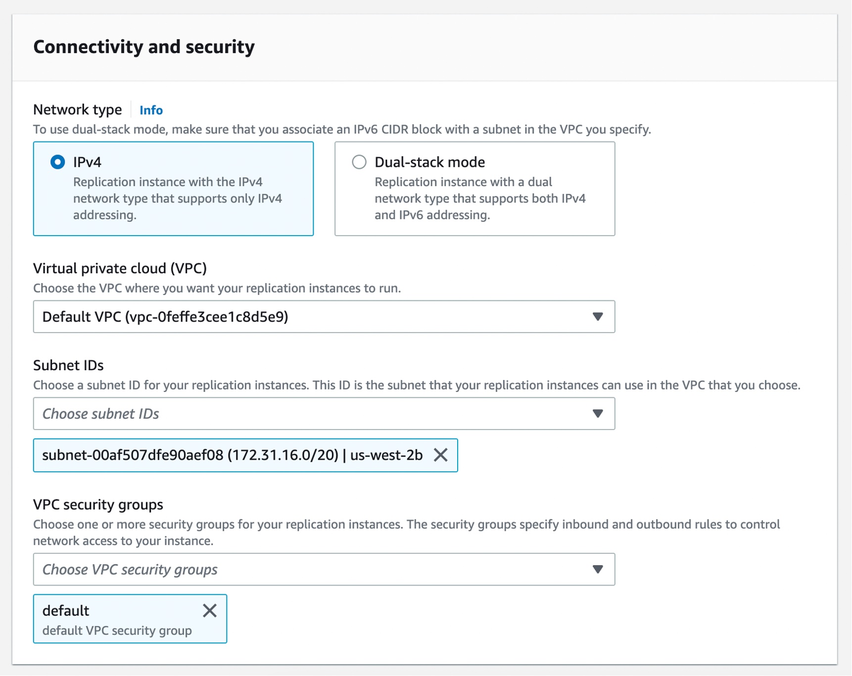
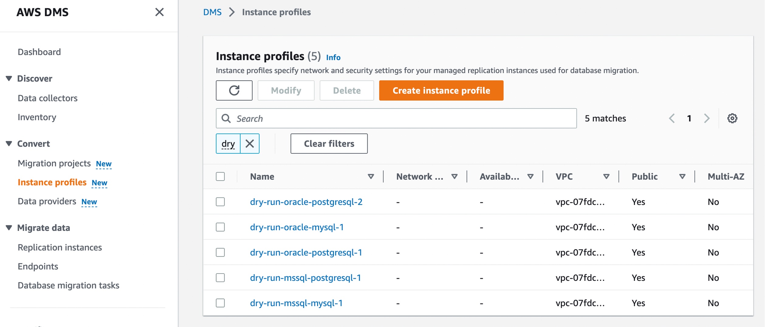
Choose Create instance profile and specify your default VPC or a new VPC, Amazon Simple Storage Service (Amazon S3) bucket to store your schema conversion metadata, and additional settings such as AWS Key Management Service (AWS KMS) keys.

You can create the simplest network configuration with a single VPC configuration. If your source or target data providers are in different VPCs, you can create your instance profile in one of the VPCs, and then link these two VPCs by using VPC peering.

Next, you can add data providers that store the data store type and location information about your source and target databases by choosing Data providers in the left pane. For each database, you can create a single data provider and use it in multiple migration projects.

Your data provider can be a fully managed Amazon RDS instance or a self-managed engine running either on-premises or on an Amazon Elastic Compute Cloud (Amazon EC2) instance.

Choose Create data provider to create a new data provider. You can set the type of the database location manually, such as database engine, domain name or IP address, port number, database name, and so on, for your data provider. Here, I have selected an RDS database instance.

After you create a data provider, make sure that you add database connection credentials in AWS Secrets Manager. DMS Schema Conversion uses this information to connect to a database.

Converting your database schema with AWS DMS Schema Conversion
Now, you can create a migration project for DMS Schema Conversion by choosing Migration projects in the left pane. A migration project describes your source and target data providers, your instance profile, and migration rules. You can also create multiple migration projects for different source and target data providers.

Choose Create migration project and select your instance profile and source and target data providers for DMS Schema Conversion.

After creating your migration project, you can use the project to create assessment reports and convert your database schema. Choose your migration project from the list, then choose the Schema conversion tab and click Launch schema conversion.

Migration projects in DMS Schema Conversion are always serverless. This means that AWS DMS automatically provisions the cloud resources for your migration projects, so you don’t need to manage schema conversion instances.

Of course, the first launch of DMS Schema Conversion requires starting a schema conversion instance, which can take up to 10–15 minutes. This process also reads the metadata from the source and target databases. After a successful first launch, you can access DMS Schema Conversion faster.

An important part of DMS Schema Conversion is that it generates a database migration assessment report that summarizes all of the schema conversion tasks. It also details the action items for schema that cannot be converted to the DB engine of your target database instance. You can view the report in the AWS DMS console or export it as a comma-separated value (.csv) file.

To create your assessment report, choose the source database schema or schema items that you want to assess. After you select the checkboxes, choose Assess in the Actions menu in the source database pane. This report will be archived with .csv files in your S3 bucket. To change the S3 bucket, edit the schema conversion settings in your instance profile.

Then, you can apply the converted code to your target database or save it as a SQL script. To apply converted code, choose Convert in the pane of Source data provider and then Apply changes in the pane of Target data provider.

Once the schema has been converted successfully, you can move on to the database migration phase using AWS DMS. To learn more, see Getting started with AWS Database Migration Service in the AWS documentation.

Now Available
AWS DMS Schema Conversion is now available in the US East (Ohio), US East (N. Virginia), US West (Oregon), Asia Pacific (Singapore), Asia Pacific (Sydney), Asia Pacific (Tokyo), Europe (Frankfurt), Europe (Ireland), and Europe (Stockholm) Regions, and you can start using it today.

To learn more, see the AWS DMS Schema Conversion User Guide, give it a try, and please send feedback to AWS re:Post for AWS DMS or through your usual AWS support contacts.

Channy