Tag Archives: Customer Solutions

Detect Adversary Behavior in Milliseconds with CrowdStrike and Amazon EventBridge

Post Syndicated from Joby Bett original https://aws.amazon.com/blogs/architecture/detect-adversary-behavior-in-seconds-with-crowdstrike-and-amazon-eventbridge/

By integrating Amazon EventBridge with Falcon Horizon, CrowdStrike has developed a real-time, cloud-based solution that allows you to detect threats in less than a second. This solution uses AWS CloudTrail and EventBridge. CloudTrail allows governance, compliance, operational auditing, and risk auditing of your AWS account. EventBridge is a serverless event bus that makes it easier to build event-driven applications at scale.

In this blog post, we’ll cover the challenges presented by using traditional log file-based security monitoring. We will also discuss how CrowdStrike used EventBridge to create an innovative, real-time cloud security solution that enables high-speed, event-driven alerts that detect malicious actors in milliseconds.

Challenges of log file-based security monitoring

Being able to detect malicious actors in your environment is necessary to stay secure in the cloud. With the growing volume, velocity, and variety of cloud logs, log file-based monitoring makes it difficult to reveal adverse behaviors in time to stop breaches.

When an attack is in progress, a security operations center (SOC) analyst has an average of one minute to detect the threat, ten minutes to understand it, and one hour to contain it. If you cannot meet this 1/10/60 minute rule, you may have a costly breach that may move laterally and explode exponentially across the cloud estate.

Let’s look at a real-life scenario. When a malicious actor attempts a ransom attack that targets high-value data in an Amazon Simple Storage Service (Amazon S3) bucket, it can involve activities in various parts of the cloud services in a brief time window.

These example activities can involve:

  • AWS Identity and Access Management (IAM): account enumeration, disabling multi-factor authentication (MFA), account hijacking, privilege escalation, etc.
  • Amazon Elastic Compute Cloud (Amazon EC2): instance profile privilege escalation, file exchange tool installs, etc.
  • Amazon S3: bucket and object enumeration; impair bucket encryption and versioning; bucket policy manipulation; getObject, putObject, and deleteObject APIs, etc.

With siloed log file-based monitoring, detecting, understanding, and containing a ransom attack while still meeting the 1/10/60 rule is difficult. This is because log files are written in batches, and files are typically only created every 5 minutes. Once the log file is written, it still needs to be fetched and processed. This means that you lose the ability to dynamically correlate disparate activities.

To summarize, top-level challenges of log file-based monitoring are:

  1. Lag time between the breach and the detection
  2. Inability to correlate disparate activities to reveal sophisticated attack patterns
  3. Frequent false positive alarms that obscure true positives
  4. High operational cost of log file synchronizations and reprocessing
  5. Log analysis tool maintenance for fast growing log volume

Security and compliance is a shared responsibility between AWS and the customer. We protect the infrastructure that runs all of the services offered in the AWS Cloud. For abstracted services, such as  Amazon S3, we operate the infrastructure layer, the operating system, and platforms, and customers access the endpoints to store and retrieve data.

You are responsible for managing your data (including encryption options), classifying assets, and using IAM tools to apply the appropriate permissions.

Indicators of attack by CrowdStrike with Amazon EventBridge

In real-world cloud breach scenarios, timeliness of observation, detection, and remediation is critical. CrowdStrike Falcon Horizon IOA is built on an event-driven architecture based on EventBridge and operates at a velocity that can outpace attackers.

CrowdStrike Falcon Horizon IOA performs the following core actions:

  • Observe: EventBridge streams CloudTrail log files across accounts to the CrowdStrike platform as activity occurs. Parallelism is enabled via event bus rules, which enables CrowdStrike to avoid the five-minute lag in fetching the log files and dynamically correlate disparate activities. The CrowdStrike platform observes end-to-end activities from AWS services and infrastructure hosted in the accounts protected by CrowdStrike.
  • Detect: Falcon Horizon invokes indicators of attack (IOA) detection algorithms that reveal adversarial or anomalous activities from the log file streams. It correlates new and historical events in real time while enriching the events with CrowdStrike threat intelligence data. Each IOA is prioritized with the likelihood of activity being malicious via scoring and mapped to the MITRE ATT&CK framework.
  • Remediate: The detected IOA is presented with remediation steps. Depending on the score, applying the remediations quickly can be critical before the attack spreads.
  • Prevent: Unremediated insecure configurations are revealed via indicators of misconfiguration (IOM) in Falcon Horizon. Applying the remediation steps from IOM can prevent future breaches.

Key differentiators of IOA from Falcon Horizon are:

  • Observability of wider attack surfaces with heterogeneous event sources
  • Detection of sophisticated tactics, techniques, and procedures (TTPs) with dynamic event correlation
  • Event enrichment with threat intelligence that aids prioritization and reduces alert fatigue
  • Low latency between malicious activity occurrence and corresponding detection
  • Insight into attacks for each adversarial event from MITRE ATT&CK framework

High-level architecture

Event-driven architectures provide advantages for integrating varied systems over legacy log file-based approaches. For securing cloud attack surfaces against the ever-evolving TTPs, a robust event-driven architecture at scale is a key differentiator.

CrowdStrike maximizes the advantages of event-driven architecture by integrating with EventBridge, as shown in Figure 1. EventBridge allows observing CloudTrail logs in event streams. It also simplifies log centralization from a number of accounts with its direct source-to-target integration across accounts, as follows:

  1. CrowdStrike hosts an EventBridge with central event buses that consume the stream of CloudTrail log events from a multitude of customer AWS accounts.
  2. Within customer accounts, EventBridge rules listen to the local CloudTrail and stream each activity as an event to the centralized EventBridge hosted by CrowdStrike.
  3. CrowdStrike’s event-driven platform detects adversarial behaviors from the event streams in real time. The detection is performed against incoming events in conjunction with historical events. The context that comes from connecting new and historical events minimizes false positives and improves alert efficacy.
  4. Events are enriched with CrowdStrike threat intelligence data that provides additional insight of the attack to SOC analysts and incident responders.
CrowdStrike Falcon Horizon IOA architecture

Figure 1. CrowdStrike Falcon Horizon IOA architecture

As data is received by the centralized EventBridge, CrowdStrike relies on unique customer ID and AWS Region in each event to provide integrity and isolation.

EventBridge allows relatively hassle-free customer onboarding by using cross account rules to transfer customer CloudTrail data into one common event bus that can then be used to filter and selectively forward the data into the Falcon Horizon platform for analysis and mitigation.

Conclusion

As your organization’s cloud footprint grows, visibility into end-to-end activities in a timely manner is critical for maintaining a safe environment for your business to operate. EventBridge allows event-driven monitoring of CloudTrail logs at scale.

CrowdStrike Falcon Horizon IOA, powered by EventBridge, observes end-to-end cloud activities at high speeds at scale. Paired with targeted detection algorithms from in-house threat detection experts and threat intelligence data, Falcon Horizon IOA combats emerging threats against the cloud control plane with its cutting-edge event-driven architecture.

Related information

Optimizing Cloud Infrastructure Cost and Performance with Starburst on AWS

Post Syndicated from Kinnar Kumar Sen original https://aws.amazon.com/blogs/architecture/optimizing-cloud-infrastructure-cost-and-performance-with-starburst-on-aws/

Amazon Web Services (AWS) Cloud is elastic, convenient to use, easy to consume, and makes it simple to onboard workloads. Because of this simplicity, the cost associated with onboarding workloads is sometimes overlooked.

There is a notion that when an organization moves its workload to the cloud, agility, scalability, performance, and cost issues will disappear. While this may be true for agility and scalability, you must optimize your workload. You can do this with services like Amazon EC2 Auto Scaling via Amazon Elastic Compute Cloud (Amazon EC2) and Amazon EC2 Spot Instances to realize the performance and cost benefits the cloud offers.

In this blog post, we show you how Starburst Enterprise (Starburst) addressed a sudden increase in cost for their data analytics platform as they grew their internal teams and scaled out their infrastructure. After reviewing their architecture and deployments with AWS specialist architects, Starburst and AWS concluded that they could take the following steps to greatly reduce costs:

  1. Use Spot Instances to run workloads.
  2. Add Amazon EC2 Auto Scaling into their training and demonstration environments, because the Starburst platform is designed to elastically scale up and down.

For analytics workloads, when you rein in costs, you typically rein in performance. Starburst and AWS worked together to balance the cost and performance of Starburst’s data analytics platform while also harnessing the flexibility, scalability, security, and performance of the cloud.

What is Starburst Enterprise?

Starburst provides a Massively Parallel Processing SQL (MPPSQL) engine based on open source Trino. It is an analytics platform that provides the cornerstone in customers’ intelligent data mesh and offers the following benefits and services:

  • The platform gives you a single point to access, monitor, and secure your data mesh.
  • The platform gives you options for your data compute. You no longer have to wait on data migrations or extract, transform, and load (ETL), there is no vendor lock-in, and there is no need to swap out your existing analytics tools.
  • Starburst Stargate (Stargate) ensures that large jobs are completed within each data domain of your data mesh. Only the result set is retrieved from the domain.
    • Stargate reduces data output, which reduces costs and increases performance.
    • Data governance policies can also be applied uniquely in each data domain, ensuring security compliance and federation.

As shown in Figure 1, there are many connectors for input and output that ensure you experience improved performance and security.

Starburst platform

Figure 1. Starburst platform

Integrating Starburst Enterprise with AWS

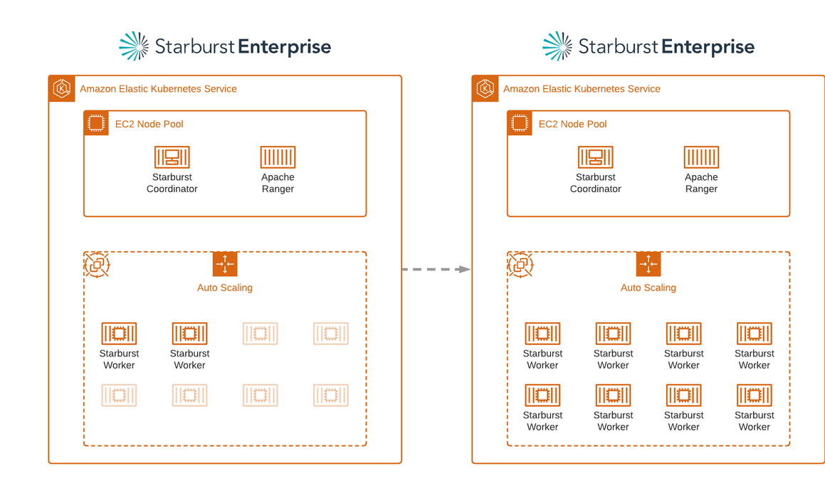
As shown in Figure 2, Starburst Enterprise uses AWS services to deliver elastic scaling and optimize cost. The platform is architected with decoupled storage and compute. This allows the platform to scale as needed to analyze petabytes of data.

The platform can be deployed via AWS CloudFormation or Amazon Elastic Kubernetes Service (Amazon EKS). Starburst on AWS allows you to run analytic queries across AWS data sources and on-premises systems such as Teradata and Oracle.

Deployment architecture of Starburst platform on AWS

Figure 2. Deployment architecture of Starburst platform on AWS

Amazon EC2 Auto Scaling

Enterprises have diverse analytic workloads; their compute and memory requirements vary with time. Starburst uses Amazon EKS and Amazon EC2 Auto Scaling to elastically scale compute resources to meet the demands of their analytics workloads.

  • Amazon EC2 Auto Scaling ensures that you have the compute capacity for your workloads to handle the load elastically. It is used to architect sophisticated, elastic, and resilient applications on the AWS Cloud.
    • Starburst uses the scheduled scaling feature of Amazon EC2 Auto Scaling to scale the cluster up/down based on time. Thus, they incur no costs when the cluster is not in use.
  • Amazon EKS is a fully managed Kubernetes service that allows you to run Kubernetes on AWS without needing to install, operate, and maintain your own Kubernetes control plane.

Scaling cloud resource consumption on demand has a major impact on controlling cloud costs. Starburst supports scaling down elastically, which means removing compute resources doesn’t impact the underlying processes.

Amazon EC2 Spot Instances

Spot Instances let you take advantage of unused EC2 capacity in the AWS Cloud. They are available at up to a 90% discount compared to On-Demand Instance prices. If EC2 needs capacity for On-Demand Instance usage, Spot Instances can be interrupted by Amazon EC2 with a two-minute notification. There are many ways to handle the interruption to ensure that the application is well architected for resilience and fault tolerance.

Starburst has integrated Spot Instances as a part of the Amazon EKS managed node groups to cost optimize the analytics workloads. This best practice of instance diversification is implemented by using the integration eksctl and instance selector with dry-run flag. This creates a list of instances of same size (vCPU/Mem ratio) and uses them in the underlying node groups.

Same size instances are required to make best use of Kubernetes Cluster Autoscaler, which is used to manage the size of the cluster.

Scaling down, handling interruptions, and provisioning compute

“Scaling in” an active application is tricky, but Starburst was built with resiliency in mind, and it can effectively manage shut downs.

Spot Instances are an ideal compute option because Starburst can handle potential interruptions natively. Starburst also uses Amazon EKS managed node groups to provision nodes in the cluster. This requires significantly less operational effort compared to using self-managed node groups. It allows Starburst to enforce best practices like capacity optimized allocation strategy, capacity rebalancing, and instance diversification.

When you need to “scale out” the deployment, Amazon EKS and Amazon EC2 Auto Scaling help to provision capacity, as depicted in Figure 3.

Depicting “scale out” in a Starburst deployment

Figure 3. Depicting “scale out” in a Starburst deployment

Benefits realized from using AWS services

In a short period, Starburst was able to increase the number of people working on AWS. They added five times the number of Solutions Architects, they have previously. Additionally, in their initial tests of their new deployment architecture, their Solutions Architects were able to complete up to three times the amount of work than they had been able to previously. Even after the workload increased more than 15 times, with two simple changes they only had a slight increase in total cost.

This cost and performance optimization allows Starburst to be more productive internally and realize value for each dollar spent. This further justified investing more into building out infrastructure footprint.

Conclusion

In building their architecture with AWS, Starburst realized the importance of having a robust and comprehensive cloud administration plan that they can implement and manage going forward. They are now able to balance the cloud costs with performance and stability, even after considering the SLA requirements. Starburst is planning to teach their customers about the Spot Instance and Amazon EC2 Auto Scaling best practices to ensure they maintain a cost and performance optimized cloud architecture.

If you want to see the Starburst data analytics platform in action, you can get a free trial in the AWS Marketplace: Starburst Data Free Trial.

How Rapid7 built multi-tenant analytics with Amazon Redshift using near-real-time datasets

Post Syndicated from Rahul Monga original https://aws.amazon.com/blogs/big-data/how-rapid7-built-multi-tenant-analytics-with-amazon-redshift-using-near-real-time-datasets/

This is a guest post co-written by Rahul Monga, Principal Software Engineer at Rapid7.

Rapid7 InsightVM is a vulnerability assessment and management product that provides visibility into the risks present across an organization. It equips you with the reporting, automation, and integrations needed to prioritize and fix those vulnerabilities in a fast and efficient manner. InsightVM has more than 5,000 customers across the globe, runs exclusively on AWS, and is available for purchase on AWS Marketplace.

To provide near-real-time insights to InsightVM customers, Rapid7 has recently undertaken a project to enhance the dashboards in their multi-tenant software as a service (SaaS) portal with metrics, trends, and aggregated statistics on vulnerability information identified in their customer assets. They chose Amazon Redshift as the data warehouse to power these dashboards due to its ability to deliver fast query performance on gigabytes to petabytes of data.

In this post, we discuss the design options that Rapid7 evaluated to build a multi-tenant data warehouse and analytics platform for InsightVM. We will deep dive into the challenges and solutions related to ingesting near-real-time datasets and how to create a scalable reporting solution that can efficiently run queries across more than 3 trillion rows. This post also discusses an option to address the scenario where a particular customer outgrows the average data access needs.

This post uses the terms customers, tenants, and organizations interchangeably to represent Rapid7 InsightVM customers.

Background

To collect data for InsightVM, customers can use scan engines or Rapid7’s Insight Agent. Scan engines allow you to collect vulnerability data on every asset connected to a network. This data is only collected when a scan is run. Alternatively, you can install the Insight Agent on individual assets to collect and send asset change information to InsightVM numerous times each day. The agent also ensures that asset data is sent to InsightVM regardless of whether or not the asset is connected to your network.

Data from scans and agents is sent in the form of packed documents, in micro-batches of hundreds of events. Around 500 documents per second are received across customers, and each document is around 2 MB in size. On a typical day, InsightVM processes 2–3 trillion rows of vulnerability data, which translates to around 56 GB of compressed data for a large customer. This data is normalized and processed by InsightVM’s vulnerability management engine and streamed to the data warehouse system for near-real-time availability of data for analytical insights to customers.

Architecture overview

In this section, we discuss the overall architectural setup for the InsightVM system.

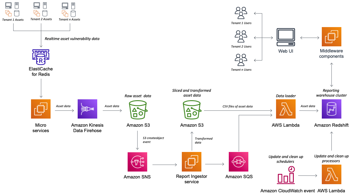
Scan engines and agents collect and send asset information to the InsightVM cloud. Asset data is pooled, normalized, and processed to identify vulnerabilities. This is stored in an Amazon ElastiCache for Redis cluster and also pushed to Amazon Kinesis Data Firehouse for use in near-real time by InsightVM’s analytics dashboards. Kinesis Data Firehose delivers raw asset data to an Amazon Simple Storage Service (Amazon S3) bucket. The data is transformed using a custom developed ingestor service and stored in a new S3 bucket. The transformed data is then loaded into the Redshift data warehouse. Amazon Simple Notification Service (Amazon SNS), Amazon Simple Queue Service (Amazon SQS), and AWS Lambda are used to orchestrate this data flow.  In addition, to identify the latest timestamp of vulnerability data for assets, an auxiliary table is maintained and updated periodically with the update logic in the Lambda function, which is triggered through an Amazon CloudWatch event rule. Custom-built middleware components interface between the web user interface (UI) and the Amazon Redshift cluster to fetch asset information for display in dashboards.

The following diagram shows the implementation architecture of InsightVM, including the data warehouse system:

Rapid-7 Multi-tenant Architecture

The architecture has built-in tenant isolation because data access is abstracted through the API. The application uses a dimensional model to support low-latency queries and extensibility for future enhancements.

Amazon Redshift data warehouse design: Options evaluated and selection

Considering Rapid7’s need for near-real-time analytics at any scale, the InsightVM data warehouse system is designed to meet the following requirements:

  • Ability to view asset vulnerability data at near-real time, within 5–10 minutes of ingest
  • Less than 5 seconds’ latency when measured at 95 percentiles (p95) for reporting queries
  • Ability to support 15 concurrent queries per second, with the option to support more in the future
  • Simple and easy-to-manage data warehouse infrastructure
  • Data isolation for each customer or tenant

Rapid7 evaluated Amazon Redshift RA3 instances to support these requirements. When designing the Amazon Redshift schema to support these goals, they evaluated the following strategies:

  • Bridge model – Storage and access to data for each tenant is controlled at the individual schema level in the same database. In this approach, multiple schemas are set up, where each schema is associated with a tenant, with the same exact structure of the dimensional model.
  • Pool model – Data is stored in a single database schema for all tenants, and a new column (tenant_id) is used to scope and control access to individual tenant data. Access to the multi-tenant data is controlled using API-level access to the tables. Tenants aren’t aware of the underlying implementation of the analytical system and can’t query them directly.

For more information about multi-tenant models, see Implementing multi-tenant patterns in Amazon Redshift using data sharing.

Initially when evaluating the bridge model, it provided an advantage for tenant-only data for queries, plus the ability to decouple a tenant to an independent cluster if they outgrow the resources that are available in the single cluster. Also, when the p95 metrics were evaluated in this setup, the query response times were less than 5 seconds, because each tenant data is isolated into smaller tables. However, the major concern with this approach was with the near-real-time data ingestion into over 50,000 tables (5,000 customer schemas x approximately 10 tables per schema) every 5 minutes. Having thousands of commits every minute into an online analytical processing (OLAP) system like Amazon Redshift can lead to most resources being exhausted in the ingestion process. As a result, the application suffers query latencies as data grows.

The pool model provides a simpler setup, but the concern was with query latencies when multiple tenants access the application from the same tables. Rapid7 hoped that these concerns would be addressed by using Amazon Redshift’s support for massively parallel processing (MPP) to enable fast execution of most complex queries operating on large amounts of data. With the right table design using the right sort and distribution keys, it’s possible to optimize the setup. Furthermore, with automatic table optimization, the Amazon Redshift cluster can automatically make these determinations without any manual input.

Rapid7 evaluated both the pool and bridge model designs, and decided to implement the pool model. This model provides simplified data ingestion and can support query latencies of under 5 seconds at p95 with the right table design. The following table summarizes the results of p95 tests conducted with the pool model setup.

Query P95
Large customer: Query with multiple joins, which list assets, their vulnerabilities, and all their related attributes, with aggregated metrics for each asset, and filters to scope assets by attributes like location, names, and addresses Less than 4 seconds
Large customer: Query to return vulnerability content information given a list of vulnerability identifiers Less than 4 seconds

Tenet isolation and security

Tenant isolation is fundamental to the design and development of SaaS systems. It enables SaaS providers to reassure customers that, even in a multi-tenant environment, their resources can’t be accessed by other tenants.

With the Amazon Redshift table design using the pool model, Rapid7 built a separate data access layer in the middleware that templatized queries, augmented with runtime parameter substitution to uniquely filter specific tenant and organization data.

The following is a sample of templatized query:

<#if useDefaultVersion()>
currentAssetInstances AS (
SELECT tablename.*
FROM tablename
<#if (applyTags())>
JOIN dim_asset_tag USING (organization_id, attribute2, attribute3)
</#if>
WHERE organization_id ${getOrgIdFilter()}
<#if (applyTags())>
AND tag_id IN ($(tagIds))
</#if>
),
</#if>

The following is a Java interface snippet to populate the template:

public interface TemplateParameters {

boolean useDefaultVersion(); boolean useVersion(); default Set<String> getVersions() {
return null;
} default String getVersionJoin(String var1) {
return "";
}

String getTemplateName();

String getOrgIdString();

default String getOrgIdFilter() {
return "";
}

Every query uses organization_id and additional parameters to uniquely access tenant data. During runtime, organization_id and other metadata are extracted from the secured JWT token that is passed to middleware components after the user is authenticated in the Rapid7 cloud platform.

Best practices and lessons learned

To fully realize the benefits of the Amazon Redshift architecture and design for the multiple tenants & near real-time ingestion, considerations on the table design allow you to take full advantage of the massively parallel processing and columnar data storage. In this section, we discuss the best practices and lessons learned from building this solution.

Sort key for effective data pruning

Sorting a table on an appropriate sort key can accelerate query performance, especially queries with range-restricted predicates, by requiring fewer table blocks to be read from disk. To have Amazon Redshift choose the appropriate sort order, the AUTO option was utilized. Automatic table optimization continuously observes how queries interact with tables and discovers the right sort key for the table. To effectively prune the data by the tenant, organization_id is identified as the sort key to perform the restricted scans. Furthermore, because all queries are routed through the data access layer, organization_id is automatically added in the predicate conditions to ensure effective use of the sort keys.

Micro-batches for data ingestion

Amazon Redshift is designed for large data ingestion, rather than transaction processing. The cost of commits is relatively high, and excessive use of commits can result in queries waiting for access to the commit queue. Data is micro-batched during ingestion as it arrives for multiple organizations. This results in fewer transactions and commits when ingesting the data.

Load data in bulk

If you use multiple concurrent COPY commands to load one table from multiple files, Amazon Redshift is forced to perform a serialized load, and this type of load is much slower.

The Amazon Redshift manifest file is used to ingest the datasets that span multiple files in a single COPY command, which allows fast ingestion of data in each micro-batch.

RA3 instances for data sharing

Rapid 7 uses Amazon Redshift RA3 instances, which enable data sharing to allow you to securely and easily share live data across Amazon Redshift clusters for reads. In this multi-tenant architecture when a tenant outgrows the average data access needs, it can be isolated to a separate cluster easily and independently scaled using the data sharing. This is accomplished by monitoring the STL_SCAN table to identify different tenants and isolate them to allow for independent scalability as needed.

Concurrency scaling for consistently fast query performance

When concurrency scaling is enabled, Amazon Redshift automatically adds additional cluster capacity when you need it to process an increase in concurrent read queries. To meet the uptick in user requests, the concurrency scaling feature is enabled to dynamically bring up additional capacity to provide consistent p95 values that meet Rapid7’s defined requirements for the InsightVM application.

Results and benefits

Rapid7 saw the following results from this architecture:

  • The new architecture has reduced the time required to make data accessible to customers to less than 5 minutes on average. The previous architecture had higher level of processing time variance, and could sometimes exceed 45 minutes
  • Dashboards load faster and have enhanced drill-down functionality, improving the end-user experience
  • With all data in a single warehouse, InsightVM has a single source of truth, compared to the previous solution where InsightVM had copies of data maintained in different databases and domains, which could occasionally get out of sync
  • The new architecture lowers InsightVM’s reporting infrastructure cost by almost three times, as compared to the previous architecture

Conclusion

With Amazon Redshift, the Rapid7 team has been able to centralize asset and vulnerability information for InsightVM customers. The team has simultaneously met its performance and management objectives with the use of a multi-tenant pool model and optimized table design. In addition, data ingestion via Kinesis Data Firehose and custom-built microservices to load data into Amazon Redshift in near-real time enabled Rapid7 to deliver asset vulnerability information to customers more than nine times faster than before, improving the InsightVM customer experience.


About the Authors

Rahul Monga is a Principal Software Engineer at Rapid7, currently working on the next iteration of InsightVM. Rahul’s focus areas are highly distributed cloud architectures and big data processing. Originally from the Washington DC area, Rahul now resides in Austin, TX with his wife, daughter, and adopted pup.

Sujatha Kuppuraju is a Senior Solutions Architect at Amazon Web Services (AWS). She works with ISV customers to help design secured, scalable and well-architected solutions on the AWS Cloud. She is passionate about solving complex business problems with the ever-growing capabilities of technology.

Thiyagarajan Arumugam is a Principal Solutions Architect at Amazon Web Services and designs customer architectures to process data at scale. Prior to AWS, he built data warehouse solutions at Amazon.com. In his free time, he enjoys all outdoor sports and practices the Indian classical drum mridangam.

How Amazon CodeGuru Reviewer helps Gridium maintain a high quality codebase

Post Syndicated from Aaqib Bickiya original https://aws.amazon.com/blogs/devops/codeguru-gridium-maintain-codebase/

Gridium creates software that lets people run commercial buildings at a lower cost and with less energy. Currently, half of the world lives in cities. Soon, nearly 70% will, while buildings utilize 40% of the world’s electricity. In the U.S. alone, commercial real estate value tops one trillion dollars. Furthermore, much of this asset class is still run with spreadsheets, clipboards, and outdated software. Gridium’s software platform collects large amounts of operational data from commercial buildings like offices, medical providers, and corporate campuses. Then, our analytics identifies energy savings opportunities that we work with customers to actualize.

Gridium’s Challenge

Data streams from utility companies across the U.S. are an essential input for Gridium’s analytics. This data is processed and visualized so that our customers can garner new insights and drive smarter decisions. In order to integrate a new data source into our platform, we often utilize third-party contractors to write tools that ingest data feeds and prepare them for analysis.

Our team firmly emphasizes our codebase quality. We strive for our code to be stylistically consistent, easily testable, swiftly understood, and well-documented. We write code internally by using agreed-upon standards. This makes it easy for us to review and edit internal code using standard collaboration tools.

We work to ensure that code arriving from contractors meets similar standards, but enforcing external code quality can be difficult. Contractor-developed code will be written in the style of each contractor. Furthermore, reviewing and editing code written by contractors introduces new challenges beyond those of working with internal code. We have used tools like PyLint to help stylistically align code, but we wanted a method for uncovering more complex issues without burdening the team and undermining the benefits of outside contractors.

Adopting Amazon CodeGuru Reviewer

We began evaluating Amazon CodeGuru Reviewer in order to provide an additional review layer for code developed by contractors, and to find complex corrections within code that traditional tools might not catch.

Initially, we enabled the service only on external repositories and generated reviews on pull requests. CodeGuru immediately provided us with actionable recommendations for maintaining Gridium’s codebase quality.

CodeGuru exception handling correction

The example above demonstrates a useful recurring recommendation related to exception-handling. Strictly speaking, there is nothing wrong with utilizing a general Exception class whenever needed. However, utilizing general Exception classes in production can complicate error-handling functions and generate ambiguity when trying to debug or understand code.

After a few weeks of utilizing CodeGuru Reviewer and witnessing its benefits, we determined that we wanted to use it for our entire codebase. Moreover, CodeGuru provided us with meaningful recommendations on our internal repositories.

CodeGuru highly depend functions suggestions

This example once again showcases CodeGuru’s ability to highlight subtle issues that aren’t necessarily bugs. Without diving through related libraries and functions, it would be difficult to find any optimizable areas, but CodeGuru found that this function could become problematic due to its dependency on twenty other functions. If any of the dependencies is updated, then it could break the entire function, thereby making debugging the root cause difficult.

The explanations following each code recommendation were essential in our quick adoption of CodeGuru. Simply showing what code to change would make it tough to follow through with a code correction. CodeGuru provided ample context, reasoning, and even metrics in some cases to explain and justify a correction.

Conclusion

Our development team thoroughly appreciates the extra review layer that CodeGuru provides. CodeGuru indicates areas that internal review might otherwise miss, especially in code written by external contractors.

In some cases, CodeGuru highlighted issues never before considered by the team. Examples of these issues include highly coupled functions, ambiguous exceptions, and outdated API calls. Each suggestion is accompanied with its context and reasoning so that our developers can independently judge if an edit should be made. Furthermore, CodeGuru was easily set up with our GitHub repositories. We enabled it within minutes through the console.

After familiarizing ourselves with the CodeGuru workflow, Gridium treats CodeGuru recommendations like suggestions that an internal reviewer would make. Both internal developers and third parties act on recommendations in order to improve code health and quality. Any CodeGuru suggestions not accepted by contractors are verified and implemented by an internal reviewer if necessary.

Over the twelve weeks that we have been utilizing Amazon CodeGuru, we have had 281 automated pull request reviews. These provided 104 recommendations resulting in fifty code corrections that we may not have made otherwise. Our monthly bill for CodeGuru usage is about $10.00. If we make only a single correction to our code over a whole month that we would have missed otherwise, then we can safely say that it was well worth the price!

About the Authors

Kimberly Nicholls is an Engineering Technical Lead at Gridium who loves to make data useful. She also enjoys reading books and spending time outside.

Adnan Bilwani is a Sr. Specialist-Builder Experience providing fully managed ML-based solutions to enhance your DevOps workflows.

Aaqib Bickiya is a Solutions Architect at Amazon Web Services. He helps customers in the Midwest build and grow their AWS environments.

How The Mill Adventure Implemented Event Sourcing at Scale Using DynamoDB

Post Syndicated from Uri Segev original https://aws.amazon.com/blogs/architecture/how-the-mill-adventure-implemented-event-sourcing-at-scale-using-dynamodb/

This post was co-written by Joao Dias, Chief Architect at The Mill Adventure and Uri Segev, Principal Serverless Solutions Architect at AWS

The Mill Adventure provides a complete gaming platform, including licenses and operations, for rapid deployment and success in online gaming. It underpins every aspect of the process so that you can focus on telling your story to your audience while the team makes everything else work perfectly.

In this blog post, we demonstrate how The Mill Adventure implemented event sourcing at scale using Amazon DynamoDB and Serverless on AWS technologies. By partnering with AWS, The Mill Adventure reduced their costs, and they are able to maintain operations and scale their solution to suit their needs without their intervention.

What is event sourcing?

Event sourcing captures an entity’s state (such as a transaction or a user) as a sequence of state-changing events. Whenever the state changes, a new event is appended to the sequence of events using an atomic operation.

The system persists these events in an event store, which is a database of events. The store supports adding and retrieving the state events. The system reconstructs the entity’s state by reading the events from the event store and replaying them. Because the store is immutable (meaning these events are saved in the event store forever) the entity’s state can be recreated up to a particular version or date and have accurate historical values.

Why use event sourcing?

Event sourcing provides many advantages, that include (but are not limited to) the following:

  • Audit trail: Events are immutable and provide a history of what has taken place in the system. This means it’s not only providing the current state, but how it got there.
  • Time travel: By persisting a sequence of events, it is relatively easy to determine the state of the system at any point in time by aggregating the events within that time period. This provides you the ability to answer historical questions about the state of the system.
  • Performance: Events are simple and immutable and only require an append operation. The event store should be optimized to handle high-performance writes.
  • Scalability: Storing events avoids the complications associated with saving complex domain aggregates to relational databases, which allows more flexibility for scaling.

Event-driven architectures

Event sourcing is also related to event-driven architectures. Every event that changes an entity’s state can also be used to notify other components about the change. In event-driven architectures, we use event routers to distribute the events to interested components.

The event router has three main functions:

  1. Decouple the event producers from the event consumers: The producers don’t know who the consumers are, and they do not need to change when new consumers are added or removed.
  2. Fan out: Event routers are capable of distributing events to multiple subscribers.
  3. Filtering: Event routers send each subscriber only the events they are interested in. This saves on the number of events that consumers need to process; therefore, it reduces the cost of the consumers.

How did The Mill Adventure implement event sourcing?

The Mill Adventure uses DynamoDB tables as their object store. Each event is a new item in the table. The DynamoDB table model for an event sourced system is quite simple, as follows:

Field Type Description
id PK The object identifier
version SK The event sequence number
eventdata The event data itself, in other words, the change to the object’s state

All events for the same object have the same id. Thus, you can retrieve them using a single read request.

When a component modifies the state of an object, it first determines the sequence number for the new event by reading the current state from the table (in other words, the sequence of events for that object). It then attempts to write a new item to the table that represents the change to the object’s state. The item is written using DynamoDB’s conditional write. This ensures that there are no other changes to the same object happening at the same time. If the write failed due to a condition not met error, it will start over.

An additional benefit of using DynamoDB as the event store is DynamoDB Streams, which is used to deliver events about changes in tables. These events can be used by event-driven applications so they will know about the different objects’ change of state.

How does it work?

Let’s use an example of a business entity, such as a user. When a user is created, the system creates a UserCreated event with the initial user data (like user name, address, etc.). The system then persists this event to the DynamoDB event store using a conditional write. This makes sure that the event is only written once and that the version numbers are sequential.

Then the user address gets updated, so again, the system creates a UserUpdated event with the new address and persists it.

When the system needs the user’s current state, for example, to show it in back-office application, the system loads all the events for the given user identifier from the store. For each one of them, it invokes a mutation function that recreates the latest state. Given the following items in the database:

  • Event 1: UserCreated(name: The Mill, address: Malta)
  • Event 2: UserUpdated(address: World)

You can imagine how each mutator function for those events would look like, which then produce the latest state:

{ 
"name": "The Mill", 
"address": "World" 
}

A business state like a bank statement can have a large number of events. To optimize loading, the system periodically saves a snapshot of the current state. To reconstruct the current state, the application finds the most recent snapshot and the events that have occurred since that snapshot. As a result, there are fewer events to replay.

Architecture

The Mill Adventure architecture for an event source system using AWS components is straightforward. The architecture is fully serverless, as such, it only uses AWS Lambda functions for compute. Lambda functions produce the state-changing events that are written to the database.

Other Lambda functions, when they retrieve an object’s state, will read the events from the database and calculate the current state by replaying the events.

Finally, interested functions will be notified about the changes by subscribing to the event bus. Then they perform their business logic, like updating state projections or publishing to WebSocket APIs. These functions use DynamoDB streams as the event bus to handle messages as shows in Figure 1.

Event sourcing architecture

Figure 1. Event sourcing architecture

Figure 1 is not completely accurate due to a limitation of DynamoDB Streams, which can only support up to two subscribers.

Because The Mill Adventure has many microservices that are interested in these events, they have a single function that gets invoked from the stream and sends the events to other event routers. These fan out to a large number of subscribers such as Amazon EventBridge, Amazon Simple Notification Service (Amazon SNS), or maybe even Amazon Kinesis Data Streams for some use cases.

Any service in the system could be listening to these events being created via the DynamoDB stream and distributed via the event router and act on them. For example, publishing a WebSocket API notification or prompting a contact update in a third-party service.

Conclusion

In this blog post, we showed how The Mill Adventure uses serverless technologies like DynamoDB and Lambda functions to implement an event-driven event sourcing system.

An event sourced system can be difficult to scale, but using DynamoDB as the event store resolved this issue. It can also be difficult to produce consistent snapshots and Command Query Responsibility Segregation (CQRS) views, but using DynamoDB streams for distributing the events made it relatively easy.

By partnering with AWS, The Mill Adventure created a sports/casino platform to be proud of. It provides high quality data and performance without having servers, they only pay for what they use, and their workload can scale up and down as needed.

How MOIA built a fully automated GDPR compliant data lake using AWS Lake Formation, AWS Glue, and AWS CodePipeline

Post Syndicated from Leonardo Pêpe original https://aws.amazon.com/blogs/big-data/how-moia-built-a-fully-automated-gdpr-compliant-data-lake-using-aws-lake-formation-aws-glue-and-aws-codepipeline/

This is a guest blog post co-written by Leonardo Pêpe, a Data Engineer at MOIA.

MOIA is an independent company of the Volkswagen Group with locations in Berlin and Hamburg, and operates its own ride pooling services in Hamburg and Hanover. The company was founded in 2016 and develops mobility services independently or in partnership with cities and existing transport systems. MOIA’s focus is on ride pooling and the holistic development of the software and hardware for it. In October 2017, MOIA started a pilot project in Hanover to test a ride pooling service, which was brought into public operation in July 2018. MOIA covers the entire value chain in the area of ​​ride pooling. MOIA has developed a ridesharing system to avoid individual car traffic and use the road infrastructure more efficiently.

In this post, we discuss how MOIA uses AWS Lake Formation, AWS Glue, and AWS CodePipeline to store and process gigabytes of data on a daily basis to serve 20 different teams with individual user data access and implement fine-grained control of the data lake to comply with General Data Protection Regulation (GDPR) guidelines. This involves controlling access to data at a granular level. The solution enables MOIA’s fast pace of innovation to automatically adapt user permissions to new tables and datasets as they become available.

Background

Each MOIA vehicle can carry six passengers. Customers interact with the MOIA app to book a trip, cancel a trip, and give feedback. The highly distributed system prepares multiple offers to reach their destination with different pickup points and prices. Customers select an option and are picked up from their chosen location. All interactions between the customers and the app, as well as all the interactions between internal components and systems (the backend’s and vehicle’s IoT components), are sent to MOIA’s data lake.

Data from the vehicle, app, and backend must be centralized to have the synchronization between trips planned and implemented, and then to collect passenger feedback. To provide different pricing and routing options, MOIA needed centralized data. MOIA decided to build and secure its Amazon Simple Storage Service (Amazon S3) based Data Lake using AWS Lake Formation.

Different MOIA teams that includes Data Analysts, Data Scientists and Data Engineers need to access centralized data from different sources for the development and operations of the application workloads. It’s a legal requirement to control the access and format of the data to these different teams. The app development team needs to understand customer feedback in an anonymized way, pricing-related data must be accessed only by the business analytics team, vehicle data is meant to be used only by the vehicle maintenance team, and the routing team needs access to customer location and destination.

Architecture overview

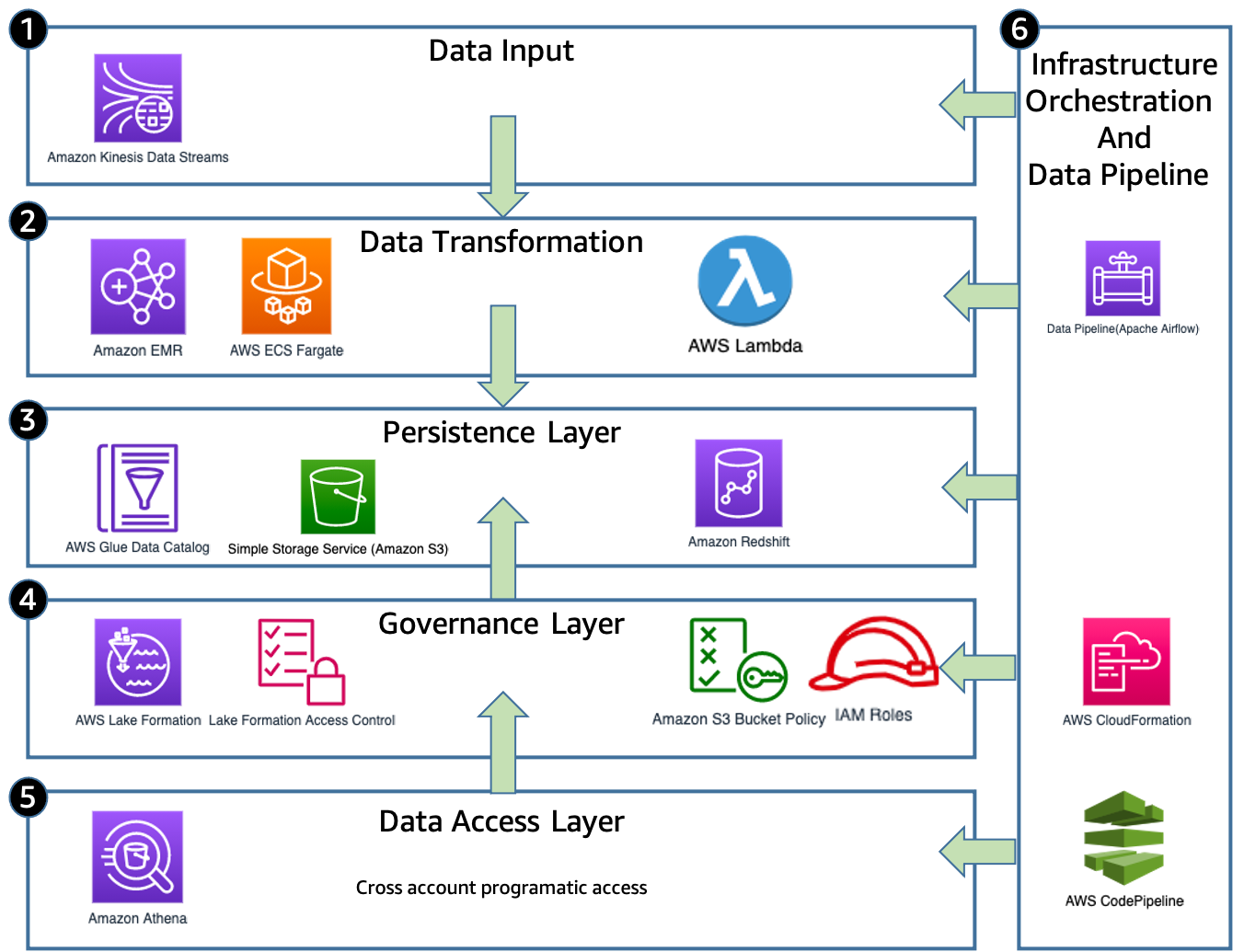
The following diagram illustrates MOIA solution architecture.

The solution has the following components:

  1. Data input – The apps, backend, and IoT devices are continuously streaming event messages via Amazon Kinesis Data Streams in a nested information in a JSON format.
  2. Data transformation – When the raw data is received, the data pipeline orchestrator (Apache Airflow) starts the data transformation jobs to meet requirements for respective data formats. Amazon EMR, AWS Lambda, or AWS Fargate cleans, transforms, and loads the events in the S3 data lake.
  3. Persistence layer – After the data is transformed and normalized, AWS Glue crawlers classify the data to determine the format, schema, and associated properties. They group data into tables or partitions and write metadata to the AWS Glue Data Catalog based on the structured partitions created in Amazon S3. The data is written on Amazon S3 partitioned by its event type and timestamp so it can be easily accessed via Amazon Athena and the correct permissions can be applied using Lake Formation. The crawlers are run at a fixed interval in accordance with the batch jobs, so no manual runs are required.
  4. Governance layer – Access on the data lake is managed using the Lake Formation governance layer. MOIA uses Lake Formation to centrally define security, governance, and auditing policies in one place. These policies are consistently implemented, which eliminates the need to manually configure them across security services like AWS Identity and Access Management (IAM), AWS Key Management Service (AWS KMS), storage services like Amazon S3, or analytics and machine learning (ML) services like Amazon Redshift, Athena, Amazon EMR for Apache Spark. Lake Formation reduces the effort in configuring policies across services and provides consistent assistance for GDPR requirements and compliance. When a user makes a request to access Data Catalog resources or underlying data from the data lake, for the request to succeed, it must pass permission checks by both IAM and Lake Formation. Lake Formation permissions control access to Data Catalog resources, Amazon S3 locations, and the underlying data at those locations. User permissions to the data on the table, row, or column level are defined in Lake Formation, so that users only access the data if they’re authorized.
  5. Data access layer – After the flattened and structured data is available to be accessed by the data analysts, scientists, and engineers they can use Amazon Redshift or Athena to perform SQL analysis, or AWS Data Wrangler and Apache Spark to perform programmatic analysis and build ML use cases.
  6. Infrastructure orchestration and data pipeline – After the data is ingested and transformed, the infrastructure orchestration layer (CodePipeline and Lake Formation) creates or updates the governance layer with the proper and predefined permissions periodically every hour (see more about the automation in the governance layer later in this post).

Governance challenge

MOIA wants to evolve their ML models for routing, demand prediction, and business models continuously. This requires MOIA to constantly review models and update them, therefore power users such as data administrators and engineers frequently redesign the table schemas in the AWS Glue Data Catalog as part of the data engineering workflow. This highly dynamic metadata transformation requires an equally dynamic governance layer pipeline that can assign the right user permissions to all tables and adapt to these changes transparently without disruptions to end-users. Due to GDPR requirements, there is no room for error, and manual work is required to assign the right permissions according to GDPR compliance on the tables in the data lake with many terabytes of data. Without automation, many developers are needed for administration; this adds human error into the workflows, which is not acceptable. Manual administration and access management isn’t a scalable solution. MOIA needed to innovate faster with GDPR compliance with a small team of developers.

Data schema and data structure often changes at MOIA, resulting in new tables being created in the data lake. To guarantee that new tables inherit the permissions granted to the same group of users who already have access to the entire database, MOIA uses an automated process that grants Lake Formation permission to newly created tables, columns, and databases, as described in the next section.

Solution overview

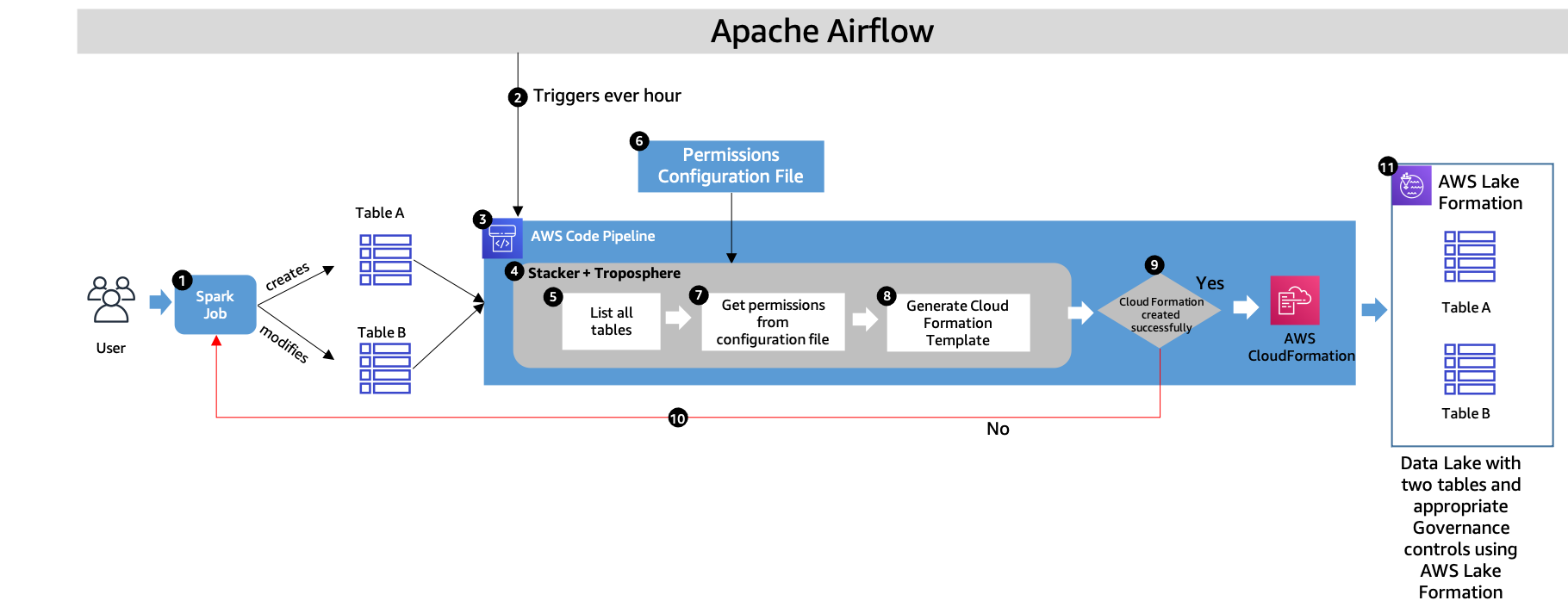
The following diagram illustrates the continuous deployment loop using AWS CloudFormation.

The workflow contains the following steps:

  1. MOIA data scientists and engineers create or modify new tables to evolve the business and ML models. This results in new tables or changes in the existing schema of the table.
  2. The data pipeline is orchestrated via Apache Airflow, which controls the whole cycle of ingestion, cleansing, and data transformation using Spark jobs (as shown in Step 1). When the data is in its desired format and state, Apache Airflow triggers the AWS Glue crawler job to discover the data schema in the S3 bucket and add the new partitions to the Data Catalog. Apache Airflow also triggers CodePipeline to assign the right permissions on all the tables.
  3. Apache Airflow triggers CodePipeline every hour, which uses MOIA’s libraries to discover the new tables, columns, and databases, and grants Lake Formation permissions in the AWS CloudFormation template for all tables, including new and modified. This orchestration layer ensures Lake Formation permissions are granted. Without this step, nobody can access new tables, and new data isn’t visible to data scientists, business analysts, and others who need it.
  4. MOIA uses Stacker and Troposphere to identify all the tables, assign the tables the right permissions, and deploy the CloudFormation stack. Troposphere is the infrastructure as code (IaC) framework that renders the CloudFormation templates, and stacker helps with the parameterization and deployment of the templates on AWS. Stacker also helps produce reusable templates in the form of blueprints as pure Python code, which can be easily parameterized using YAML files. The Python code uses Boto3 clients to lookup the Data Catalog and search for databases and tables.
  5. The stacker blueprint libraries developed by MOIA (which internally use Boto3 and troposphere) are used to discover newly created databases or tables in the Data Catalog.
  6. A Permissions configuration file allows MOIA to predefine data lake tables (Can be a wildcard indicating all tables available in one database) and specific personas who have access to these tables. These roles are split into different categories called lake personas, and have specific access levels. Example lake personas include data domain engineers, data domain technical users, data administrators, and data analysts. Users and their permissions are defined in the file. In case access to personally identifiable information (PII) data is granted, the GDPR officer ensures that a record of processing activities is in place and the usage of personal data is documented according to the law.
  7. MOIA uses stacker to read the predefined permissions file, and uses the customized stacker blueprints library containing the logic to assign permissions to lake personas for each of the tables discovered in Step 5.
  8. The discovered and modified tables are matched with predefined permissions in Step 6 and Step 7. Stacker uses YAML format as the input for the CloudFormation template parameters to define users and data access permissions. These parameters are related to the user’s roles and define access to the tables. Based on this, MOIA creates a customized stacker that creates AWS CloudFormation resources dynamically. The following are the example stacks in AWS CloudFormation:
    1. data-lake-domain-database – Holds all resources that are relevant during the creation of the database, which includes lake permissions at the database level that allow the domain database admin personas to perform operations in the database.
    2. data-lake-domain-crawler – Scans Amazon S3 constantly to discover and create new tables and updates.
    3. data-lake-lake-table-permissions – Uses Boto3 combined with troposphere to list the available tables and grant lake permissions to the domain roles that access it.

This way, new CloudFormation templates are created, containing permissions for new or modified tables. This process guarantees a fully automated governance layer for the data lake. The generated CloudFormation template contains Lake Formation permission resources for each table, database, or column. The process of managing Lake Formation permissions on Data Catalog databases, tables, and columns is simplified by granting Data Catalog permissions using the Lake Formation tag-based access control method. The advantage of generating a CloudFormation template is audibility. When the new version of the CloudFormation stack is prepared with an access control set on new or modified tables, administrators can compare that stack with the older version to discover newly prepared and modified tables. MOIA can view the differences via the AWS CloudFormation console before new stack deployment.

  1. Either the CloudFormation stack is deployed in the account with the right permissions for all users, or a stack deployment failure notice is sent to the developers via a Slack channel (Step 10). This ensures the visibility in the deployment process and failed pipelines in permission assignment.
  2. Whenever the pipeline fails, MOIA receives the notification via Slack so the engineers can promptly fix the errors. This loop is very important to guarantee that whenever the schema changes, those changes are reflected in the data lake without manual intervention.
  3. Following this automated pipeline, all the tables are assigned right permissions.

Benefits

This solution delivers the following benefits:

  • Automated enforcement of data access permissions allows people to access the data without manual interventions in a scalable way. With automation, 1,000 hours of manual work are saved every year.
  • The GDPR team does the assessment internally every month. The GDPR team constantly provides guidance and approves each change in permissions. This audit trail for records of processing activities is automated with the help of Lake Formation (otherwise it needs a dedicated human resource).
  • The automated workflow of permission assignment is integrated into existing CI/CD processes, resulting in faster onboarding of new teams, features, and dataset releases. An average of 48 releases are done each month (including major and minor version releases and new event types). Onboarding new teams and forming internal new teams is very easy now.
  • This solution enables you to create a data lake using IaC processes that are easy and GDPR-compliant.

Conclusion

MOIA has created scalable, automated, and versioned permissions with a GDPR-supported, governed data lake using Lake Formation. This solution helps them bring new features and models to market faster, and reduces administrative and repetitive tasks. MOIA can focus on 48 average releases every month, contributing to a great customer experience and new data insights.


About the Authors

Leonardo Pêpe is a Data Engineer at MOIA. With a strong background in infrastructure and application support and operations, he is immersed in the DevOps philosophy. He’s helping MOIA build automated solutions for its data platform and enabling the teams to be more data-driven and agile. Outside of MOIA, Leonardo enjoys nature, Jiu-Jitsu and martial arts, and explores the good of life with his family.


Sushant Dhamnekar is a Solutions Architect at AWS. As a trusted advisor, Sushant helps automotive customers to build highly scalable, flexible, and resilient cloud architectures, and helps them follow the best practices around advanced cloud-based solutions. Outside of work, Sushant enjoys hiking, food, travel, and CrossFit workouts.


Shiv Narayanan is Global Business Development Manager for Data Lakes and Analytics solutions at AWS. He works with AWS customers across the globe to strategize, build, develop and deploy modern data platforms. Shiv loves music, travel, food and trying out new tech.

Toyota Connected and AWS Design and Deliver Collision Assistance Application

Post Syndicated from Srikanth Kodali original https://aws.amazon.com/blogs/architecture/toyota-connected-and-aws-design-and-deliver-collision-assistance-application/

This post was cowritten by Srikanth Kodali, Sr. IoT Data Architect at AWS, and Will Dombrowski, Sr. Data Engineer at Toyota Connected

Toyota Connected North America (TC) is a technology/big data company that partners with Toyota Motor Corporation and Toyota Motor North America to develop products that aim to improve the driving experience for Toyota and Lexus owners.

TC’s Mobility group provides backend cloud services that are built and hosted in AWS. Together, TC and AWS engineers designed, built, and delivered their new Collision Assistance product, which debuted in early August 2021.

In the aftermath of an accident, Collision Assistance offers Toyota and Lexus drivers instructions to help them navigate a post-collision situation. This includes documenting the accident, filing an insurance claim, and transitioning to the repair process.

In this blog post, we’ll talk about how our team designed, built, refined, and deployed the Collision Assistance product with Serverless on AWS services. We’ll discuss our goals in developing this product and the architecture we developed based on those goals. We’ll also present issues we encountered when testing our initial architecture and how we resolved them to create the final product.

Building a scalable, affordable, secure, and high performing product

We used a serverless architecture because it is often less complex than other architecture types. Our goals in developing this initial architecture were to achieve scalability, affordability, security, and high performance, as described in the following sections.

Scalability and affordability

In our initial architecture, Amazon Simple Queue Service (Amazon SQS) queues, Amazon Kinesis streams, and AWS Lambda functions allow data pipelines to run servers only when they’re needed, which introduces cost savings. They also process data in smaller units and run them in parallel, which allows data pipelines to scale up efficiently to handle peak traffic loads. These services allow for an architecture that can handle non-uniform traffic without needing additional application logic.

Security

Collision Assistance can deliver information to customers via push notifications. This data must be encrypted because many data points the application collects are sensitive, like geolocation.

To secure this data outside our private network, we use Amazon Simple Notification Service (Amazon SNS) as our delivery mechanism. Amazon SNS provides HTTPS endpoint delivery of messages coming to topics and subscriptions. AWS allows us to enable at-rest and/or in-transit encryption for all of our other architectural components as well.

Performance

To quantify our product’s performance, we review the “notification delay.” This metric evaluates the time between the initial collision and when the customer receives a push notification from Collision Assistance. Our ultimate goal is to have the push notification sent within minutes of a crash, so drivers have this information in near real time.

Initial architecture

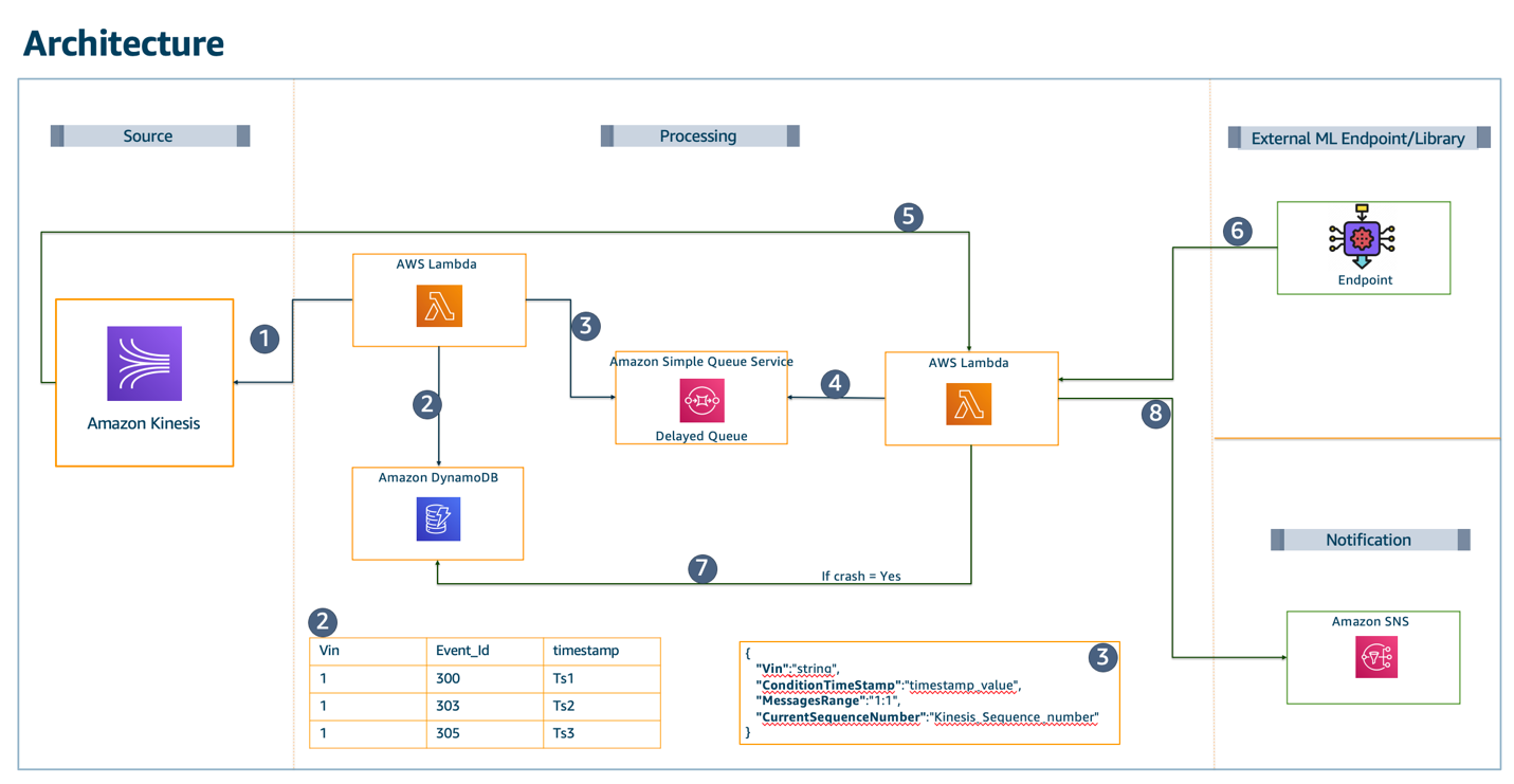
Figure 1 presents our initial architecture implementation that aims to predict whether a crash has occurred and reduce false positives through the following data pipeline:

  1. The Kinesis stream receives vehicle data from an upstream ingestion service, as discussed in the Enhancing customer safety by leveraging the scalable, secure, and cost-optimized Toyota Connected Data Lake blog.
  2. A Lambda function writes lookup data to Amazon DynamoDB for every Kinesis record.
  3. This Lambda function decreases obvious non-crash data. It sends the current record (X) to Amazon SQS. If X exceeds a certain threshold, it will remain a crash candidate.
  4. Amazon SQS sets a delivery delay so that there will be more Kinesis/DynamoDB records available when X is processed later in the pipeline.
  5. A second Lambda function reads the data from the SQS message. It queries DynamoDB to find the Kinesis lookup data for the message before (X-1) and after (X+1) the crash candidate.
  6. Kinesis GetRecords retrieves X-1 and X+1, because X+1 will exist after the SQS delivery delay times out.
  7. The X-1, X, and X+1 messages are sent to the data science (DS) engine.
  8. When a crash is accurately predicted, these results are stored in a DynamoDB table.
  9. The push notification is sent to the vehicle owner. (Note: the push notification is still in ‘select testing phase’)
Diagram and description of our initial architecture implementation

Figure 1. Diagram and description of our initial architecture implementation

To be consistent with privacy best practices and reduce server uptime, this architecture uses the minimum amount of data the DS engine needs.

We filter out records that are lower than extremely low thresholds. Once these records are filtered out, around 40% of the data fits the criteria to be evaluated further. This reduces the server capacity needed by the DS engine by 60%.

To reduce false positives, we gather data before and after the timestamps where the extremely low thresholds are exceeded. We then evaluate the sensor data across this timespan and discard any sets with patterns of abnormal sensor readings or other false positive conditions. Figure 2 shows the time window we initially used.

Longitudinal acceleration versus time

Figure 2. Longitudinal acceleration versus time

Adjusting our initial architecture for better performance

Our initial design worked well for processing a few sample messages and achieved the desired near real-time delivery of the push notification. However, when the pipeline was enabled for over 1 million vehicles, certain limits were exceeded, particularly for Kinesis and Lambda integrations:

  • Our Kinesis GetRecords API exceeded the allowed five requests per shard per second. With each crash candidate retrieving an X-1 and X+1 message, we could only evaluate two per shard per second, which isn’t cost effective.
  • Additionally, the downstream SQS-reading Lambda function was limited to 10 records per second per invocation. This meant any slowdown that occurs downstream, such as during DS engine processing, could cause the queue to back up significantly.

To improve cost and performance for the Kinesis-related functionality, we abandoned the DynamoDB lookup table and the GetRecord calls in favor of using a Redis cache cluster on Amazon ElastiCache. This allows us to avoid all throughput exceptions from Kinesis and focus on scaling the stream based on the incoming throughput alone. The ElastiCache cluster scales capacity by adding or removing shards, which improves performance and cost efficiency.

To solve the Amazon SQS/Lambda integration issue, we funneled messages directly to an additional Kinesis stream. This allows the final Lambda function to use some of the better scaling options provided to Kinesis-Lambda event source integrations, like larger batch sizes and max-parallelism.

After making these adjustments, our tests proved we could scale to millions of vehicles as needed. Figure 3 shows a diagram of this final architecture.

Final architecture

Figure 3. Final architecture

Conclusion

Engineers across many functions worked closely to deliver the Collision Assistance product.

Our team of backend Java developers, infrastructure experts, and data scientists from TC and AWS built and deployed a near real-time product that helps Toyota and Lexus drivers document crash damage, file an insurance claim, and get updates on the actual repair process.

The managed services and serverless components available on AWS provided TC with many options to test and refine our team’s architecture. This helped us find the best fit for our use case. Having this flexibility in design was a key factor in designing and delivering the best architecture for our product.


How Magellan Rx Management used Amazon Redshift ML to predict drug therapeutic conditions

Post Syndicated from Karim Prasla original https://aws.amazon.com/blogs/big-data/how-magellan-rx-management-used-amazon-redshift-ml-to-predict-drug-therapeutic-conditions/

This post is co-written with Karim Prasla and Deepti Bhanti from Magellan Rx Management as the lead authors.

Amazon Redshift ML makes it easy for data scientists, data analysts, and database developers to create, train, and use machine learning (ML) models using familiar SQL commands in Amazon Redshift data warehouses. The ML feature can be used by various personas; in this post we discuss how data analysts at Magellan Rx Management used Redshift ML to predict and classify drugs into various therapeutic conditions.

About Magellan Rx Management

Magellan Rx Management, a division of Magellan Health, Inc., is shaping the future of pharmacy. As a next-generation pharmacy organization, we deliver meaningful solutions to the people we serve. As pioneers in specialty drug management, industry leaders in Medicaid pharmacy programs, and disruptors in pharmacy benefit management, we partner with our customers and members to deliver a best-in-class healthcare experience.

Use case

Magellan Rx Management uses data and analytics to deliver clinical solutions that improve patient care, contain costs, and improve outcomes. We utilize predictive analytics to forecast future drugs costs, identify drugs that will drive future trends, including pipeline medications, and proactively identify patients at risk for becoming non-adherent to their medications.

We develop and deliver these analytics via our MRx Predict solution. This solution utilizes a variety of data, including pharmacy and medical claims, compendia information, census data, and many other sources to optimize the predictive model development, deployment, and most importantly maximize predictive accuracy.

Part of the process involves stratification of drugs and patient population based on therapeutic conditions. These conditions are derived by utilizing compendia drug attributes to come up with a classification system focused on disease categories, such as diabetes, hypertension, spinal muscular atrophy, and many others, and ensuring drugs are appropriately categorized as opposed to being included in the “miscellaneous” bucket, which is the case for many specialty medications. Also, this broader approach to classifying drugs, beyond just mechanism of action, has allowed us to effectively develop downstream reporting solutions, patient segmentation, and outcomes analytics.

Although we use different technologies for predictive analytics, we wanted to use Redshift ML to predict appropriate drug therapeutic conditions, because it would allow us to use this functionality within our Amazon Redshift data warehouse by making the predictions using standard SQL programming. Prior to Redshift ML, we had data analysts and clinicians manually categorize any new drugs into the appropriate therapeutic conditions. The end goal of using Redshift ML was to assess how well we could improve our operational efficiency while maintaining a high level of clinical accuracy.

Redshift ML allowed us to create models using standard SQL without having to use external systems, technologies, or APIs. With data already in Amazon Redshift, our data scientists and analysts, who are skilled in SQL, seamlessly created ML models to effectively predict therapeutic conditions for individual drugs.

“At Magellan Rx Management, we leverage data, analytics, and proactive insights, to help solve complex pharmacy challenges, while focusing on improving clinical and economic outcomes for customers and members,” said Karim Prasla, Vice President of Clinical Outcomes Advanced Analytics and Research at Magellan Rx Management.“We use predictive analytics and machine learning to improve operational and clinical efficiencies and effectiveness. With Redshift ML, we were able to enable our data and outcomes analysts to classify new drugs to market into appropriate therapeutic conditions by creating and utilizing ML models with minimal effort. The efficiency gained through leveraging Redshift ML to support this process improved our productivity and optimized our resources while generating a high degree of predictive accuracy.”

Magellan Rx Management continues to focus on using data analytics to identify opportunities to improve patient care and outcomes, to deliver proactive insights to our customers so sound data-driven decisions can be made, and end-user tools to allow customers and support staff to have readily available insights. By incorporating predictive analytics along with providing descriptive and diagnostic insights, we at Magellan Rx Management are able to partner with our customers to ensure we evaluate the “what,” the “why,” and the “what will” to more effectively manage the pharmacy programs.

Key benefits of using Redshift ML

Redshift ML enables you to train models with a single SQL CREATE MODEL command. The CREATE MODEL command creates a model that Amazon Redshift uses to generate model-based predictions with familiar SQL constructs.

Redshift ML provides simple, optimized, and secure integration between Amazon Redshift and Amazon SageMaker, and enables inference within the Amazon Redshift cluster, making it easy to use predictions generated by ML-based models in queries and applications. An analyst with SQL skills can easily create and train models with no expertise in ML programming languages, algorithms, and APIs.

With Redshift ML, you don’t have to perform any of the undifferentiated heavy lifting required for integrating with an external ML service. Redshift ML saves you the time to format and move data, manage permission controls, or build custom integrations, workflows, and scripts. You can easily use popular ML algorithms and simplify training needs that require frequent iteration from training to prediction. Amazon Redshift automatically discovers the best algorithm and tunes the best model for your problem. You can simply make predictions and predictive analytics from within your Amazon Redshift cluster without the need to move data out of Amazon Redshift.

Simplifying integration between Amazon Redshift and SageMaker

Before Redshift ML, a data scientist had to go through a series of steps with various tools to arrive at a prediction—identify the appropriate ML algorithms in SageMaker or use Amazon SageMaker Autopilot, export the data from the data warehouse, and prepare the training data to work with these models. When the model is deployed, the scientist goes through various iterations with new data for making predictions (also known as inference). This involves moving data back and forth between Amazon Redshift and SageMaker through a series of manual steps:

  1. Export training data to Amazon Simple Storage Service (Amazon S3).
  2. Train the model in SageMaker.
  3. Export prediction input data to Amazon S3.
  4. Generate predictions in SageMaker.
  5. Import targets back into the database.

The following diagram depicts these steps.
Amazon Redshift ML Architecture
This iterative process is time-consuming and prone to errors, and automating the data movement can take weeks or months of custom coding that then needs to be maintained.

Redshift ML enables you to use ML with your data in Amazon Redshift without this complexity. Without movement of data, you don’t have any overhead of additional security and governance of data that you export from your data warehouse.

Prerequisites

To take advantage of Redshift ML, you need an Amazon Redshift cluster with the ML feature enabled.

The cluster needs to have an AWS Identity and Access Management (IAM) role attached with sufficient privileges on Amazon S3 and SageMaker. For more information on setup and an introduction to Redshift ML, see Create, train, and deploy machine learning models in Amazon Redshift using SQL with Amazon Redshift ML. The IAM role is required for Amazon Redshift to interact with SageMaker and Amazon S3. An S3 bucket is also required to export the training dataset and store other ML-related intermediate artifacts.

Setup and data preparation

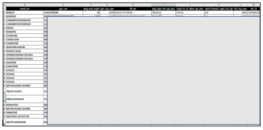
We use a sample dataset for this use case; the last column mrx_therapeutic_condition is the one we’re going to predict using the multi-classification model. We ingest this health care drug dataset into the Amazon Redshift cluster, and use it to train and test the model.

To get randomness in the training dataset, we used a random record number column (record_nbr), which can be used to separate the training dataset from testing. If your dataset already has a unique or primary key column, you can use it as a predicate to separate the training from testing dataset. The random factor (record_nbr) column was added to this dataset to serve as a WHERE clause predicate to the SELECT statement in the CREATE MODEL command (discussed later in this post). A classic example is if your prediction column is True or False, then you want to make sure that the training dataset has balanced values of both and not just True or False alone. You can achieve this by using a neutral column as a predicate, which in our case is record_nbr. After loading the data, we validated to ensure all column values are uniformly distributed for training the model. A very important factor for getting better accuracy in predictions is to use a balanced dataset for training in which the distribution of all the values is balanced and covers all characteristics.

In this example, we have kept the entire data in single table but used the WHERE predicate on the record_nbr column to differentiate the training and testing datasets.

The following is the DDL and COPY commands for this use case.

  1. Sign in to Amazon Redshift using the query editor or your preferred SQL client (DBeaver, DBVisualizer, SQL WorkbenchJ) to run the SQL statements to create the database tables.
  2. Create the schema and tables using the following DDL statements:
    --create schema
    CREATE SCHEMA drug_ml;
    
    --train table
    CREATE TABLE drug_ml.ml_drug_data
    (
    record_nbr int,
    col2 datatype,
    col3 datatype,
    etc..,
    mrx_therapeutic_condition character varying(47) 
    ) 
    DISTSTYLE EVEN;

  3. Use the COPY commands to prepare and load data for model training:
    --Load 
    COPY drug_ml.ml_drug_rs_raw
    FROM 's3://<s3bucket>/poc/drug_data_000.gz'
    IAM_ROLE 'arn:aws:iam::<AWSAccount>:role/RedshiftMLRole' 
    gzip;

Create model

Now that the data setup part is done, let’s create the model in Redshift ML. Then CREATE MODEL runs in the background and you can track progress using SHOW MODEL model_name;.

For a data analyst who is not quite conversant with machine learning, the CREATE MODEL statement is a powerhouse that offers flexibility in the number of options used to create the model. In our current use case, we haven’t passed the model type as a multi-classification model or any other options but based on the input data. The Redshift ML CREATE MODEL statement can select the correct problem type and other associated parameters using Autopilot. Multi-class classification is a problem type that predicts one of many outcomes, such as predicting a rating a customer might give for a product. In our example, we predict therapeutic conditions such as acne, anti-clotting therapy, asthma, or COPD for different patients. Data scientists and ML experts can use it to perform supervised learning to tackle problems ranging from forecasting, personalization, or customer churn prediction. See the following code:

--Create model using 130 K records (80% Training Data)
CREATE MODEL drug_ml.predict_model_drug_therapeutic_condition
FROM (
	SELECT *
	FROM drug_ml.ml_drug_data
	WHERE mrx_therapeutic_condition IS NOT NULL
		AND record_nbr < 130001
	) TARGET mrx_therapeutic_condition FUNCTION predict_drug_therapeutic_condition IAM_ROLE 'Replace with your IAM Role ARN' SETTINGS (S3_BUCKET 'Replace with your bucket name');

The target (label) in the preceding code is the mrx_therapeutic_condition column, which is used for prediction, and the function that is created out of this CREATE MODEL command is named predict_drug_therapeutic_condition.

The training data comes from the table ml_drug_data, and Autopilot automatically detects the multi-classification value model type based on input data.

Show model

The command show model model_name; is used to track the progress and also to get more details about a model (see the following example code). This section contains a representative output from SHOW MODEL after CREATE MODEL is complete. It has the inputs used in the CREATE MODEL statement with more information like model state (TRAINING, READY, FAILED) and the maximum estimated runtime it will take to finish. For better accuracy for predictions, we recommend letting the model finish to completion by increasing the default timeout value (the default is actually short for better accuracy). There is also an option to use CREATE MODEL, which lets the user limit the maximum runtime to a lower number, but the more runtime you have for CREATE MODEL, more it gets to train and iterate using multiple options before settling in on the best model.

--to show the model

SHOW MODEL drug_ml.predict_model_drug_therapeutic_condition;

The following table shows our results.

Inference

For binary and multi-class classification problems, we compute the accuracy as the model metric. We use the following formula to determine the accuracy:

accuracy = (sum (actual == predicted)/total) *100

We use the newly created function predict_drug_therapeutic_condition for the prediction and use the columns other than the target (label) as the input:

-- check accuracy
WITH infer_data AS (
SELECT mrx_therapeutic_condition AS label
,drug_ml.predict_drug_therapeutic_condition(record_nbr , brand_nm, gnrc_nm, drug_prod_strgth , gnrc_seq_num, lbl_nm , drug_dsge_fmt_typ_desc , cmpd_rte_of_admn_typ_desc , specif_thrputic_ingrd_clss_typ , hicl_seq_num, ndc_id , mfc_obsolete_dt , hcfa_termnatn_dt , specif_thrputic_ingrd_clss_desc, gpi14code, druggroup  , drugclass , drugsubclass, brandname) AS predicted,
CASE
WHEN label IS NULL
THEN 'N/A'
ELSE label
END AS actual,
CASE
WHEN actual = predicted
THEN 1::INT
ELSE 0::INT
END AS correct
FROM DRUG_ML.ML_DRUG_DATA),
aggr_data AS (
SELECT SUM(correct) AS num_correct,
COUNT(*) AS total
FROM infer_data)
SELECT (num_correct::FLOAT / total::FLOAT) AS accuracy FROM aggr_data;

--output of above query
accuracy
-------------------
0.975466558808845
(1 row)

The inference query output (0.9923 *100 = 99.23 %) matches the output from the show model command.

Let’s run the prediction query on therapeutic condition to get the count of original vs. ML-predicted values for accuracy comparison:

--check prediction 
WITH infer_data
AS (
	SELECT mrx_therapeutic_condition
		,drug_ml.predict_drug_therapeutic_condition(m.record_nbr, m.brand_nm, m.gnrc_nm, m.drug_prod_strgth, m.gnrc_seq_num, Other Params) AS predicted
	FROM "DRUG_ML"."ML_DRUG_DATA" m
	WHERE mrx_therapeutic_condition IS NOT NULL
		AND record_nbr >= 130001
	)
SELECT CASE 
		WHEN mrx_therapeutic_condition = predicted
			THEN 'Match'
		ELSE 'Un-Match'
		END AS match_ind
	,count(1) AS record_cnt
FROM infer_data
GROUP BY 1;

The following table shows our output.

Conclusion

Redshift ML allows us to develop greater efficiency and enhanced ability to generate MRx therapeutic conditions, especially when new drugs come to market. Redshift ML provides an easy and seamless platform for database users to create, train, and tune models using a SQL interface. ML capabilities empower Amazon Redshift users to create models and deploy them locally on large datasets, which was an arduous task before. Different user personas, from data analysts to advanced data science and ML experts, can take advantage of Redshift ML for machine learning based predictions and gain valuable business insights.


About the Authors

Karim Prasla, Pharm D, MS, BCPS, is a clinician and a health economist focused on optimizing use of data, analytics, and insights to improve patient care and drive positive clinical and economic outcomes. Karim leads a talented team of clinicians, economists, health outcomes scientists, and data analysts at Magellan Rx Management who are passionate about leveraging data analytics to develop products and solutions that provide proactive insights to deliver value to clinicians, customers, and members.


Deepti Bhanti, PhD, is an IT leader at Magellan Rx Management with a focus on delivering big data solutions to meet the data and analytics needs for our customers. Deepti leads a full stack team of IT engineers who are passionate about architecting and building scalable solutions while driving business value and market differentiation through technological innovations.


Rajesh Francis is a Sr. Analytics Specialist Solutions Architect at AWS. He specializes in Amazon Redshift and works with customers to build scalable analytic solutions. Rajesh worked with Magellan Rx Management to help implement a lake house architecture and leverage Redshift ML for various use cases.


Satish Sathiya is a Senior Product Engineer at Amazon Redshift. He is an avid big data enthusiast who collaborates with customers around the globe to achieve success and meet their data warehousing and data lake architecture needs. Satish worked with Magellan Rx Management to help jump start ML adoption.


Debu Panda, a principal product manager at AWS, is an industry leader in analytics, application platform, and database technologies and has more than 25 years of experience in the IT world. He was responsible for driving the Amazon Redshift ML feature and working closely with Magellan Rx Management and other customers to incorporate their feedback into the service.

How Comcast uses AWS to rapidly store and analyze large-scale telemetry data

Post Syndicated from Asser Moustafa original https://aws.amazon.com/blogs/big-data/how-comcast-uses-aws-to-rapidly-store-and-analyze-large-scale-telemetry-data/

This blog post is co-written by Russell Harlin from Comcast Corporation.

Comcast Corporation creates incredible technology and entertainment that connects millions of people to the moments and experiences that matter most. At the core of this is Comcast’s high-speed data network, providing tens of millions of customers across the country with reliable internet connectivity. This mission has become more important now than ever.

This post walks through how Comcast used AWS to rapidly store and analyze large-scale telemetry data.

Background

At Comcast, we’re constantly looking for ways to gain new insights into our network and improve the overall quality of service. Doing this effectively can involve scaling solutions to support analytics across our entire network footprint. For this particular project, we wanted an extensible and scalable solution that could process, store, and analyze telemetry reports, one per network device every 5 minutes. This data would then be used to help measure quality of experience and determine where network improvements could be made.

Scaling big data solutions is always challenging, but perhaps the biggest challenge of this project was the accelerated timeline. With 2 weeks to deliver a prototype and an additional month to scale it, we knew we couldn’t go through the traditional bake-off of different technologies, so we had to either go with technologies we were comfortable with or proven managed solutions.

For the data streaming pipeline, we already had the telemetry data coming in on an Apache Kafka topic, and had significant prior experience using Kafka combined with Apache Flink to implement and scale streaming pipelines, so we decided to go with what we knew. For the data storage and analytics, we needed a suite of solutions that could scale quickly, had plenty of support, and had an ecosystem of well-integrated tools to solve any problem that might arise. This is where AWS was able to meet our needs with technologies like Amazon Simple Storage Service (Amazon S3), AWS Glue, Amazon Athena, and Amazon Redshift.

Initial architecture

Our initial prototype architecture for the data store needed to be fast and simple so that we could unblock the development of the other elements of the budding telemetry solution. We needed three key things out of it:

  • The ability to easily fetch raw telemetry records and run more complex analytical queries
  • The capacity to integrate seamlessly with the other pieces of the pipeline
  • The possibility that it could serve as a springboard to a more scalable long-term solution

The first instinct was to explore solutions we used in the past. We had positive experiences with using nosql databases, like Cassandra, to store and serve raw data records, but it was clear these wouldn’t meet our need for running ad hoc analytical queries. Likewise, we had experience with more flexible RDBMs, like Postgres, for handling more complicated queries, but we knew that those wouldn’t scale to meet our requirement to store tens to hundreds of billions of rows. Therefore, any prototyping with one of these approaches would be considered throwaway work.

After moving on from these solutions, we quickly settled on using Amazon S3 with Athena. Amazon S3 provides low-cost storage with near-limitless scaling, so we knew we could store as much historical data as required and Athena would provide serverless, on-demand querying of our data. Additionally, Amazon S3 is known to be a launching pad to many other data store solutions both inside and outside the AWS ecosystem. This was perfect for the exploratory prototyping phase.

Integrating it into the rest of our pipeline would also prove simple. Writing the data to Amazon S3 from our Flink job was straightforward and could be done using the readily available Flink streaming file sink with an Amazon S3 bucket as the destination. When the data was available in Amazon S3, we ran AWS Glue to index our Parquet-formatted data and generate schemas in the AWS Glue metastore for searching using Athena with standard SQL.

The following diagram illustrates this architecture.

Using Amazon S3 and Athena allowed us to quickly unblock development of our Flink pipeline and ensure that the data being passed through was correct. Additionally, we used the AWS SDK to connect to Athena from our northbound Golang microservice and provide REST API access to our data for our custom web application. This allowed us to prove out an end-to-end solution with almost no upfront cost and very minimal infrastructure.

Updated architecture

As application and service development proceeded, it became apparent that Amazon Athena performed for developers running ad hoc queries, but wasn’t going to work as a long-term responsive backend for our microservices and user interface requirements.

One of the primary use cases of this solution was to look at device-level telemetry reports for a period of time and plot and track different aspects of their quality of experience. Because this most often involves solving problems happening in the now, we needed an improved data store for the most recent hot data.

This led us to Amazon Redshift. Amazon Redshift requires loading the data into a dedicated cluster and formulating a schema tuned for your use cases.

The following diagram illustrates this updated architecture.

Data loading and storage requirements

For loading and storing the data in Amazon Redshift, we had a few fundamental requirements:

  • Because our Amazon Redshift solution would be for querying data to troubleshoot problems happening as recent as the current hour, we needed to minimize the latency of the data load and keep up with our scale while doing it. We couldn’t live with nightly loads.
  • The pipeline had to be robust and recover from failures automatically.

There’s a lot of nuance that goes into making this happen, and we didn’t want to worry about handling these basic things ourselves, because this wasn’t where we were going to add value. Luckily, because we were already loading the data into Amazon S3, AWS Glue ETL satisfied these requirements and provided a fast, reliable, and scalable solution to do periodic loads from our Amazon S3 data store to our Amazon Redshift cluster.

A huge benefit of AWS Glue ETL is that it provides many opportunities to tune your ETL pipeline to meet your scaling needs. One of our biggest challenges was that we write multiple files to Amazon S3 from different regions every 5 minutes, which results in many small files. If you’re doing infrequent nightly loads, this may not pose a problem, but for our specific use case, we wanted to load data at least every hour and multiple times an hour if possible. This required some specific tuning of the default ETL job:

  • Amazon S3 list implementation – This allows the Spark job to handle files in batches and optimizes reads for a large number of files, preventing out of memory issues.
  • Pushdown predicates – This tells the load to skip listing any partitions in Amazon S3 that you know won’t be a part of the current run. For frequent loads, this can mean skipping a lot of unnecessary file listing during each job run.
  • File grouping – This allows the read from Amazon S3 to group files together in batches when reading from Amazon S3. This greatly improves performance when reading from a large number of small files.
  • AWS Glue 2.0 – When we were starting our development, only AWS Glue 1.0 was available, and we’d frequently see Spark cluster start times of over 10 minutes. This becomes problematic if you want to run the ETL job more frequently because you have to account for the cluster startup time in your trigger timings. When AWS Glue 2.0 came out, those start times consistently dropped to under 1 minute and they became a afterthought.

With these tunings, as well as increasing the parallelism of the job, we could meet our requirement of loading data multiple times an hour. This made relevant data available for analysis sooner.

Modeling, distributing, and sorting the data

Aside from getting the data into the Amazon Redshift cluster in a timely manner, the next consideration was how to model, distribute, and sort the data when it was in the cluster. For our data, we didn’t have a complex setup with tens of tables requiring extensive joins. We simply had two tables: one for the device-level telemetry records and one for records aggregated at a logical grouping.

The bulk of the initial query load would be centered around serving raw records from these tables to our web application. These types of raw record queries aren’t difficult to handle from a query standpoint, but do present challenges when dealing with tens of millions of unique devices and a report granularity of 5 minutes. So we knew we had to tune the database to handle these efficiently. Additionally, we also needed to be able to run more complex ad hoc queries, like getting daily summaries of each table so that higher-level problem areas could be more easily tracked and spotted in the network. These queries, however, were less time sensitive and could be run on an ad hoc, batch-like basis where responsiveness wasn’t as important.

The schema fields themselves were more or less one-to-one mappings from the respective Parquet schemas. The challenge came, however, in picking partition keys and sorting columns. For partition keys, we identified a logical device grouping column present in both our tables as the one column we were likely to join on. This seemed like a natural fit to partition on and had good enough cardinality that our distribution would be adequate.

For the sorting keys, we knew we’d be searching by the device identifier and the logical grouping; for the respective tables, and we knew we’d be searching temporally. So the primary identifier column of each table and the timestamp made sense to sort on. The documented sort key order suggestion was to use the timestamp column as the first value in the sort key, because it could provide dataset filtering on a specific time period. This initially worked well enough and we were able to get a performance improvement over Athena, but as we scaled and added more data, our raw record retrieval queries were rapidly slowing down. To help with this, we made two adjustments.

The first adjustment came with a change to the sort key. The first part of this involved swapping the order of the timestamp and the primary identifier column. This allowed us to filter down to the device and then search through the range of timestamps on just that device, skipping over all irrelevant devices. This provided significant performance gains and cut our raw record query times by several multiples. The second part of the sort key adjustment involved adding another column (a node-level identifier) to the beginning of the sort key. This allowed us to have one more level of data filtering, which further improved raw record query times.

One trade-off made while making these sort key adjustments was that our more complex aggregation queries had a noticeable decline in performance. This was because they were typically run across the entire footprint of devices and could no longer filter as easily based on time being the first column in the sort key. Fortunately, because these were less frequent and could be run offline if necessary, this performance trade-off was considered acceptable.

If the frequency of these workloads increases, we can use materialized views in Amazon Redshift, which can help avoid unnecessary reruns of the complex aggregations if minimal-to-no data changes in the underlying base tables have occurred since the last run.

The final adjustment was cluster scaling. We chose to use the Amazon Redshift next-generation RA3 nodes for a number of benefits, but three especially key benefits:

  • RA3 clusters allow for practically unlimited storage in our cluster.
  • The RA3 ability to scale storage and compute independently paired really well with our expectations and use cases. We fully expected our Amazon Redshift storage footprint to continue to grow, as well as the number, shape, and sizes of our use cases and users, but data and workloads wouldn’t necessarily grow in lockstep. Being able to scale the cluster’s compute power independent of storage (or vice versa) was a key technical requirement and cost-optimization for us.
  • RA3 clusters come with Amazon Redshift managed storage, which places the burden on Amazon Redshift to automatically situate data based on its temperature for consistently peak performance. With managed storage, hot data was cached on a large local SSD cache in each node, and cold data was kept in the Amazon Redshift persistent store on Amazon S3.

After conducting performance benchmarks, we determined that our cluster was under-powered for the amount of data and workloads it was serving, and we would benefit from greater distribution and parallelism (compute power). We easily resized our Amazon Redshift cluster to double the number of nodes within minutes, and immediately saw a significant performance boost. With this, we were able to recognize that as our data and workloads scaled, so too should our cluster.

Looking forward, we expect that there will be a relatively small population of ad hoc and experimental workloads that will require access to additional datasets sitting in our data lake, outside of Amazon Redshift in our data lake—workloads similar to the Athena workloads we previously observed. To serve that small customer base, we can leverage Amazon Redshift Spectrum, which empowers users to run SQL queries on external tables in our data lake, similar to SQL queries on any other table within Amazon Redshift, while allowing us to keep costs as lean as possible.

This final architecture provided us with the solid foundation of price, performance, and flexibility for our current set of analytical use cases—and, just as important, the future use cases that haven’t shown themselves yet.

Summary

This post details how Comcast leveraged AWS data store technologies to prototype and scale the serving and analysis of large-scale telemetry data. We hope to continue to scale the solution as our customer base grows. We’re currently working on identifying more telemetry-related metrics to give us increased insight into our network and deliver the best quality of experience possible to our customers.


About the Authors

Russell Harlin is a Senior Software Engineer at Comcast based out of the San Francisco Bay Area. He works in the Network and Communications Engineering group designing and implementing data streaming and analytics solutions.


Asser Moustafa is an Analytics Specialist Solutions Architect at AWS based out of Dallas, Texas. He advises customers in the Americas on their Amazon Redshift and data lake architectures and migrations, starting from the POC stage to actual production deployment and maintenance


Amit Kalawat is a Senior Solutions Architect at Amazon Web Services based out of New York. He works with enterprise customers as they transform their business and journey to the cloud.

Automating Your Home with Grafana and Siemens Controllers

Post Syndicated from Viktoria Semaan original https://aws.amazon.com/blogs/architecture/automating-your-home-with-grafana-and-siemens-controllers/

Imagine that you have access to a digital twin of your house that allows you to remotely monitor and control different devices inside your home. Forgot to turn off the heater or air conditioning? Didn’t close water faucets? Wondering how long your kids have been watching TV? Wouldn’t it be nice to have all the information from multiple devices in a single place?

Nowadays, many of us have smart things at home, such as thermostats, security cameras, wireless sensors, switches, etc. The problem is that most of these smart things come with different mobile applications. To get a full picture, we end up switching between applications that serve limited needs.

In this blog, we explain how to use Siemens controllers, AWS IoT, and the open-source visualization platform Grafana to quickly build a digital twin of any processes. This includes home automation, industrial applications, security systems, and others. As an example, we will monitor environmental conditions, including temperature and humidity sensors, thermostat settings, light switches, as well as monthly water and energy consumption. We will go through the architecture and steps required to integrate different building components to store data for historical analysis, enable voice control, and create interactive near real-time dashboards showing a digital representation of your house. If you would like to learn more about the solution, we will provide links to all the architecture components and detailed configuration steps.

Smart home automation solution with Siemens LOGO! compact controller

Figure 1. Smart home automation solution with Siemens LOGO! compact controller

Architecture

In this solution overview, we are using a low-cost Siemens LOGO! controller (hardware version 8.3 or higher). This controller supports traditional industrial protocols such as Simatic S7 and Modbus TCP/IP as well as MQTT through the native AWS IoT Core interface. Automation controllers are the brains behind smart systems that allow orchestrating all the devices in your home. This reference architecture can be extended to other devices that support MQTT protocol, have programmatic APIs, or Software Development Kits (SDKs). It could serve as a starting point for building a home automation solution using AWS IoT and Grafana and further customized based on customer needs.

Reference architecture for smart home automation solution

Figure 2. Reference architecture for smart home automation solution

The components of this solution are:

  • The LOGO! controller controls home automation equipment and ingests data to AWS IoT Core.
  • AWS IoT Core collects data at scale and routes messages to multiple AWS services.
  • AWS Lambda is called inside the AWS IoT Core statement to transform the incoming data prior to ingestion.
  • Amazon Timestream stores time series data and optimizes it for fast analytical queries.
  • AWS IoT SiteWise models and stores data from equipment for large scale deployments.
  • Grafana installed on Amazon Elastic Compute Cloud (Amazon EC2) visualizes data in near real-time using interactive dashboards.
  • The Alexa Skills Kit (ASK) allows interaction with devices using voice commands.
Remote monitoring dashboard allows homeowners to view and control conditions

Figure 3. Remote monitoring dashboard allows homeowners to view and control conditions

Solution overview

Step 1: Ingest data to AWS IoT

The IoT-enabled LOGO! controller provides the out-of-box capability to send data to AWS IoT Core service. In a few clicks, you can configure variables and their update frequency to be published to the AWS Cloud. To get started with the LOGO! controller, please refer to Siemens E-learning portal. AWS IoT Core collects and processes messages from remote devices transmitted over the secured MQTT protocol.

The LOGO! controller publishes data to AWS IoT Core in hexadecimal format. The Lambda function converts the data from hexadecimal to the standard decimal numeric system. If your home automation equipment sends data in the standard decimal format, then AWS IoT Core can directly write data to other AWS services without Lambda.

Step 2: Store data in Timestream or AWS IoT SiteWise

The ingested IoT data is saved for historical analysis. Timestream is a serverless time series database service that is optimized for high throughput ingestion and has built-in analytical functions. It is one of the options you can use to store IoT data. Time series is a common data format to observe how things are changing over time and it is suitable for building IoT applications.

AWS IoT SiteWise is an alternative option to store and organize data at scale. It is beneficial for large-scale commercial building automation and management systems, including offices, hotels, and factories. You can structure data by using built-in asset modeling capabilities.

Step 3: Visualize data in Grafana dashboard

Once data is stored, it can be made available to multiple applications. Grafana is a data visualization platform that you can use to monitor data. It supports near real-time visualization with a refresh rate of 5 seconds or higher. You can visualize data from multiple AWS sources (such as AWS IoT SiteWise, Timestream, and Amazon CloudWatch) and other data sources with a single Grafana dashboard. Grafana can be installed on an Amazon Linux system, Windows, macOS, or deployed on Kubernetes (K8S) or Docker containers. For customers who don’t want to manage infrastructure and are interested in developing completely serverless solution, Amazon offers an Amazon Managed Service for Grafana. At the time of writing this post, this service is available in preview with a limited number of supported plugins.

To build Grafana dashboard and retrieve data from Timestream, you can use SQL queries. Timestream query example to retrieve humidity values and timestamps for the past 24 hours:

SELECT measure_value::double as humidity, time FROM "myhome_db"."livingroom" WHERE measure_name='humidity' and time >=ago(1d)

To retrieve data from AWS IoT SiteWise, you can select asset properties from the asset navigation tab, which makes it simple for non-technical users to build dashboards.

Grafana dashboard configuration with AWS IoT SiteWise

Figure 4. Grafana dashboard configuration with AWS IoT SiteWise

One of the common issues of operational dashboards is that it’s hard to get a physical representation by looking at a cluster of multiple readings. To reflect conditions of physical assets, the information from sensors must be overlaid on top of original physical objects. ImageIt Panel Plugin for Grafana allows you to overcome this issue. You can upload a picture of your house or a system and drag sensor readings to their exact locations, thus creating digital representations of physical objects.

Step 4: Control using Alexa

Using the Alexa Skills Kit, you can build voice skills to be used on devices enabled by Alexa globally. Alexa and AWS IoT enables you to create an end-to-end voice-controlled experience without using any additional hardware. Instead, your functions run on the cloud only when you invoke Alexa with voice commands.

The easiest way to build a custom Alexa skill is to use a Lambda function. You can upload the code for your Alexa skill to a Lambda function. The code will execute in response to Alexa voice interactions and send commands to the LOGO! controller.

Conclusion

In this blog, we reviewed how you can create a digital twin of your home automation or industrial systems using Siemens controllers, AWS IoT, and Grafana dashboards. Connecting the LOGO! controller to AWS gives it access to the Internet of Things (IoT) and opens many potential applications such as anomaly detection, predictive maintenance, intrusion detection, and others.

How GE Healthcare modernized their data platform using a Lake House Architecture

Post Syndicated from Krishna Prakash original https://aws.amazon.com/blogs/big-data/how-ge-healthcare-modernized-their-data-platform-using-a-lake-house-architecture/

GE Healthcare (GEHC) operates as a subsidiary of General Electric. The company is headquartered in the US and serves customers in over 160 countries. As a leading global medical technology, diagnostics, and digital solutions innovator, GE Healthcare enables clinicians to make faster, more informed decisions through intelligent devices, data analytics, applications, and services, supported by its Edison intelligence platform.

GE Healthcare’s legacy enterprise analytics platform used a traditional Postgres based on-premise data warehouse from a big data vendor to run a significant part of its analytics workloads. The data warehouse is key for GE Healthcare; it enables users across units to gather data and generate the daily reports and insights required to run key business functions. In the last few years, the number of teams accessing the cluster increased by almost three times, with twice the initial number of users running four times the number of daily queries for which the cluster had been designed. The legacy data warehouse wasn’t able to scale to support GE Healthcare’s business needs and would require significant investment to maintain, update, and secure.

Searching for a modern data platform

After working for several years in a database-focused approach, the rapid growth in the data made the GEHC’s on-prem system unviable from a cost and maintenance perspective. This presented GE Healthcare with an opportunity to take a holistic look at the emerging and strategic needs for data and analytics. With this in mind, GE Healthcare decided to adopt a Lake House Architecture using AWS services:

  • Use Amazon Simple Storage Service (Amazon S3) to store raw enterprise and event data
  • Use familiar SQL statements to combine and process data across all data stores in Amazon S3 and Amazon Redshift
  • Apply the “best fit” concept of using the appropriate AWS technology to meet specific business needs

Architecture

The following diagram illustrates GE Healthcare’s architecture.

Choosing Amazon Redshift for the enterprise cloud data warehouse

Choosing the right data store is just as important as how you collect the data for analytics. Amazon Redshift provided the best value because it was easy to launch, access, and store data, and could scale to meet our business needs on demand. The following are a few additional reasons for why GE Healthcare made Amazon Redshift our cloud data warehouse:

  • The ability to store petabyte-scale data in Amazon S3 and query the data in Amazon S3 and Amazon Redshift with little preprocessing was important because GE Healthcare’s data needs are expanding at a significant pace.
  • The AWS based strategy provides financial flexibility. GE Healthcare moved from a fixed cost/fixed asset on-premises model to a consumption-based model. In addition, the total cost of ownership (TCO) of the AWS based architecture was less than the solution it was replacing.
  • Native integration with the AWS Analytics ecosystem made it easier to handle end-to-end analytics workflows without friction. GE Healthcare took a hybrid approach to extract, transform, and load (ETL) jobs by using a combination of AWS Glue, Amazon Redshift SQL, and stored procedures based on complexity, scale, and cost.
  • The resilient platform makes recovery from failure easier, with errors further down the pipeline less likely to affect production environments because all historical data is on Amazon S3.
  • The idea of a Lake House Architecture is that taking a one-size-fits-all approach to analytics eventually leads to compromises. It’s not simply about integrating a data lake with a data warehouse, but rather about integrating a data lake, a data warehouse, and purpose-built data stores and enabling unified governance and easy data movement. (For more information about the Lake House Architecture, see Harness the power of your data with AWS Analytics.)
  • It’s easy to implement new capabilities to support emerging business needs such as artificial intelligence, machine learning, graph databases, and more because of the extensive product capabilities of AWS and the Amazon Redshift Lake House Architecture.

Implementation steps and best practices

As part of this journey, GE Healthcare partnered with AWS Professional Services to accelerate their momentum. AWS Professional Services was instrumental in following the Working Backwards (WB) process, which is Amazon’s customer-centric product development process.

Here’s how it worked:

  • AWS Professional Services guided GE Healthcare and partner teams through the Lake House Architecture, sharing AWS standards and best practices.
  • The teams accelerated Amazon Redshift stored procedure migration, including data structure selection and table design.
  • The teams delivered performant code at scale to enable a timely go live.
  • They implemented a framework for batch file extract to support downstream data consumption via a data as a service (DaaS) solution.

Conclusion

Modernizing to a Lake House Architecture with Amazon Redshift allowed GEHC to speed up, innovate faster, and better solve customers’ needs. At the time of writing, GE Healthcare workloads are running at full scale in production. We retired our on-premises infrastructure. Amazon Redshift RA3 instances with managed storage enabled us to scale compute and storage separately based on our customers’ needs. Furthermore, with the concurrency scaling feature of Amazon Redshift, we don’t have to worry about peak times affecting user performance any more. Amazon Redshift scales out and in automatically.

We also look forward to realizing the benefits of Amazon Redshift data sharing and AQUA (Advanced Query Accelerator) for Amazon Redshift as we continue to increase the performance and scale of our Amazon Redshift data warehouse. We appreciate AWS’s continual innovation on behalf of its customers.


About the Authors

Krishna Prakash (KP) Bhat is a Sr. Director in Data & Analytics at GE Healthcare. In this role, he’s responsible for architecture and data management of data and analytics solutions within GE Healthcare Digital Technologies Organization. In his spare time, KP enjoys spending time with family. Connect him on LinkedIn.


Suresh Patnam is a Solutions Architect at AWS, specialized in big data and AI/ML. He works with customers in their journey to the cloud with a focus on big data, data lakes, and AI/ML. In his spare time, Suresh enjoys playing tennis and spending time with his family. Connect him on LinkedIn.

Synchronize and control your Amazon Redshift clusters maintenance windows

Post Syndicated from Ahmed Gamaleldin original https://aws.amazon.com/blogs/big-data/synchronize-and-control-your-amazon-redshift-clusters-maintenance-windows/

Amazon Redshift is a data warehouse that can expand to exabyte-scale. Today, tens of thousands of AWS customers (including NTT DOCOMO, Finra, and Johnson & Johnson) use Amazon Redshift to run mission-critical business intelligence dashboards, analyze real-time streaming data, and run predictive analytics jobs.

Amazon Redshift powers analytical workloads for Fortune 500 companies, startups, and everything in between. With the constant increase in generated data, Amazon Redshift customers continue to achieve successes in delivering better service to their end-users, improving their products, and running an efficient and effective business. Availability, therefore, is key in continuing to drive customer success, and AWS will use commercially reasonable efforts to make Amazon Redshift available with a Monthly Uptime Percentage for each multi-node cluster, during any monthly billing cycle, of at least 99.9% (our “Service Commitment”).

In this post, we present a solution to help you provide a predictable and repeatable experience to your Amazon Redshift end-users by taking control of recurring Amazon Redshift maintenance windows.

Amazon Redshift maintenance windows

Amazon Redshift periodically performs maintenance to apply fixes, enhancements, and new features to your cluster. This type of maintenance occurs during a 30-minute maintenance window set by default per Region from an 8-hour block on a random day of the week. You should change the scheduled maintenance window according to your business needs by modifying the cluster, either programmatically or by using the Amazon Redshift console. The window must be at least 30 minutes and not longer than 24 hours. For more information, see Managing clusters using the console.

If a maintenance event is scheduled for a given week, it starts during the assigned 30-minute maintenance window. While Amazon Redshift performs maintenance, it terminates any queries or other operations that are in progress. If there are no maintenance tasks to perform during the scheduled maintenance window, your cluster continues to operate normally until the next scheduled maintenance window. Amazon Redshift uses Amazon Simple Notification Service (Amazon SNS) to send notifications of Amazon Redshift events. You enable notifications by creating an Amazon Redshift event subscription. You can create an Amazon Redshift event notification subscription so you can be notified when an event occurs for a given cluster.

When an Amazon Redshift cluster is scheduled for maintenance, you receive an Amazon Redshift “Pending” event, as described in the following table.

Amazon Redshift category Event ID Event severity Description
Pending REDSHIFT-EVENT-2025 INFO Your database for cluster <cluster name> will be updated between <start time> and <end time>. Your cluster will not be accessible. Plan accordingly.
Pending REDSHIFT-EVENT-2026 INFO Your cluster <cluster name> will be updated between <start time> and <end time>. Your cluster will not be accessible. Plan accordingly.

Amazon Redshift also gives you the option to reschedule your cluster’s maintenance window by deferring your upcoming maintenance by up to 45 days. This option is particularly helpful if you want to maximize your cluster uptime by deferring a future maintenance window. For example, if your cluster’s maintenance window is set to Wednesday 8:30–9:00 UTC and you need to have nonstop access to your cluster for the next 2 weeks, you can defer maintenance to a date 2 weeks from now. We don’t perform any maintenance on your cluster when you have specified a deferment.

Deferring a maintenance window doesn’t apply to mandatory Amazon Redshift updates, such as vital security patches. Scheduled maintenance is different from Amazon Redshift mandatory maintenance. If Amazon Redshift needs to update hardware or make other mandatory updates during your period of deferment, we notify you and make the required changes. Your cluster isn’t available during these updates and such maintenance can’t be deferred. If a hardware replacement is required, you receive an event notification through the AWS Management Console and your SNS subscription as a “Pending” item, as shown in the following table.

Amazon Redshift category Event ID Event severity Description
Pending REDSHIFT-EVENT-3601 INFO A node on your cluster <cluster name> will be replaced between <start time> and <end time>. You can’t defer this maintenance. Plan accordingly.
Pending REDSHIFT-EVENT-3602 INFO A node on your cluster <cluster name> is scheduled to be replaced between <start time> and <end time>. Your cluster will not be accessible. Plan accordingly.

Challenge

As the number of the Amazon Redshift clusters you manage for an analytics application grows, the end-user experience becomes highly dependent on recurring maintenance. This means that you want to make sure maintenance windows across all clusters happen at the same time and fall on the same day each month. You want to avoid a situation in which, for example, your five Amazon Redshift clusters are each updated on a different day or week. Ultimately, you want to give your Amazon Redshift end-users an uninterrupted number of days where the clusters aren’t subject to any scheduled maintenance. This gives you the opportunity to announce a scheduled maintenance to your users well ahead of the maintenance date.

Amazon Redshift clusters are scheduled for maintenance depending on several factors, including when a cluster was created and its Region. For example, you may have two clusters on the same Amazon Redshift version that are scheduled for different maintenance windows. Regions implement the Amazon Redshift latest versions and patches at different times. A cluster running in us-east-1 might be scheduled for the same maintenance 1 week before another cluster in eu-west-1. This makes it harder for you to provide your end-users with a predictable maintenance schedule.

To solve this issue, you typically need to frequently check and synchronize the maintenance windows across all your clusters to a specific time, for example sat:06:00-sat:06:30. Additionally, you want to avoid having your clusters scheduled for maintenance at different intervals. For that, you need to defer maintenance across all your clusters to fall on the same exact day. For example, you can defer all maintenance across all clusters to happen 1 month from now regardless of when the cluster was last updated. This way you know that your clusters aren’t scheduled for maintenance for the next 30 days. This gives you enough time to announce the maintenance schedule to your Amazon Redshift users.

Solution overview

Having one day per month when Amazon Redshift scheduled maintenance occurs across all your clusters provides your users with a seamless experience. It gives you control and predictability over when clusters aren’t available. You can announce this maintenance window ahead of time to avoid sudden interruptions.

The following solution deploys an AWS Lambda function (RedshiftMaintenanceSynchronizer) to your AWS account. The function runs on a schedule configurable through an AWS CloudFormation template parameter frequency to run every 6, 12, or 24 hours. This function synchronizes maintenance schedules across all your Amazon Redshift clusters to happen at the same time on the same day. It also gives you the option to defer all future maintenance windows across all clusters by a number of days (deferment days) for up to 45 days. This enables you to provide your users with an uninterrupted number of days when your clusters aren’t subject to maintenance.

We use the following input parameters:

  • Deferment days – The number of days to defer all future scheduled maintenance windows. Amazon Redshift can defer maintenance windows by up to 45 days. The solution adds this number to the date of the last successfully completed maintenance across any of your clusters. The resulting date is the new maintenance date for all your clusters.
  • Frequency – The frequency to run this solution. You can configure it to run every 6, 12, or 24 hours.
  • Day – The preferred day of the week to schedule maintenance windows.
  • Hour – The preferred hour of the day to schedule maintenance windows (24-hour format).
  • Minute – The preferred minute of the hour to schedule maintenance windows.

The Lambda function performs the following steps:

  1. Lists all your Amazon Redshift clusters in the Region.
  2. Updates the maintenance window for all clusters to the same value of the day/hour/minute input parameters from the CloudFormation template.
  3. Checks for the last successfully completed maintenance across all clusters.
  4. Calculates the deferment maintenance date by adding the deferment input parameter to the date of the last successfully completed maintenance. For example, if the deferment parameter is 30 days and the last successful maintenance window completed on July 1, 2020, then the next deferment maintenance date is July 31, 2020.
  5. Defers the next maintenance window across all clusters to the deferment date calculated in the previous step.

Launch the solution

To get started, deploy the cloudFormation template to your AWS account.

  1. For Stack name, enter a name for your stack for easy reference.
  2. For Day, choose the day of week for the maintenance window to occur.
  3. For Hour, choose the hour for the window to start.
  4. For Minute, choose the minute within the hour for the window to start.

Your window should be a time with the least cluster activity and during off-peak work hours.

  1. For Deferment Days, choose the number of days to defer all future scheduled maintenance windows.
  2. For Solution Run Frequency, choose the frequency of 6, 12, or 24 hours.

cloudFormation Template

After the template has successfully deployed, the following resources are available:

  • The RedshiftMaintenanceSync Lambda function. This is a Python 3.8 Lambda function that syncs and defers the maintenance windows across all your Amazon Redshift clusters.

lamda_console

  • The RedshiftMaintenanceSyncEventRule Amazon CloudWatch event rule. This rule triggers on a schedule based on the Frequency input parameter. It triggers the RedshiftMaintenanceSync Lambda function to run the solution logic.

When the Lambda function starts and detects an already available deferment on any of your clusters, it doesn’t attempt to modify the existing deferment, and exits instead.

The solution logs any deferment it performs on any cluster in the associated CloudWatch log group.

Synchronize and defer maintenance windows

To demonstrate this solution, I have two Amazon Redshift clusters with different preferred maintenance windows and scheduled intervals.

Cluster A (see the following screenshot) has a preferred maintenance window set to Friday at 4:30–5:00 PM. It’s scheduled for maintenance in 2 days.

Cluster B has a preferred maintenance window set to Tuesday at 9:45–10:15 AM. It’s scheduled for maintenance in 6 days.

This means that my Amazon Redshift users have a 30-minute interruption twice in the next 2 and 6 days. Also, these interruptions happen at completely different times.

Let’s launch the solution and see how the cluster maintenance windows and scheduling intervals change.

The Lambda function does the following every time it runs:

  1. Lists all the clusters.
  2. Checks if any of the clusters have a deferment enabled and exits if it finds any.
  3. Syncs all preferred maintenance windows across all clusters to fall on the same time and day of week.
  4. Checks for the latest successfully completed maintenance date.
  5. Adds the deferment days to the last maintenance date. This becomes the new deferment date.
  6. Applies the new deferment date to all clusters.

Cluster A’s maintenance window was synced to the input parameters I passed to the CloudFormation template. Additionally, the next maintenance window was deferred until June 21, 2021, 8:06 AM (UTC +02:00).

Cluster B’s maintenance window is also synced to the same value from Cluster A, and the next maintenance window was deferred to the same exact day as Cluster A: June 21, 2021, 8:06 AM (UTC +02:00).

Finally, let’s check the CloudWatch log group to understand what the solution did.

Now both clusters have the same maintenance window and next scheduled maintenance, which is a month from now. In a production scenario, this gives you enough lead time to announce the maintenance window to your Amazon Redshift end-users and provide them with the exact day and time when clusters aren’t available.

Summary

This solution can help you provide a predictable and repeatable experience to your Amazon Redshift end-users by taking control of recurring Amazon Redshift maintenance windows. It enables you to provide your users with an uninterrupted number of days where clusters are always available—barring any scheduled mandatory upgrades. Click here to get started with Amazon Redshift today.


About the Author

Ahmed_Gamaleldin

Ahmed Gamaleldin is a Senior Technical Account Manager (TAM) at Amazon Web Services. Ahmed helps customers run optimized workloads on AWS and make the best out of their cloud journey.

Field Notes: How Sportradar Accelerated Data Recovery Using AWS Services

Post Syndicated from Mithil Prasad original https://aws.amazon.com/blogs/architecture/field-notes-how-sportradar-accelerated-data-recovery-using-aws-services/

This post was co-written by Mithil Prasad, AWS Senior Customer Solutions Manager, Patrick Gryczkat, AWS Solutions Architect, Ben Burdsall, CTO at Sportradar and Justin Shreve, Director of Engineering at Sportradar. 

Ransomware is a type of malware which encrypts data, effectively locking those affected by it out of their own data and requesting a payment to decrypt the data.  The frequency of ransomware attacks has increased over the past year, with local governments, hospitals, and private companies experiencing cases of ransomware.

For Sportradar, providing their customers with access to high quality sports data and insights is central to their business. Ensuring that their systems are designed securely and in a way which minimizes the possibility of a ransomware attack is top priority.  While ransomware attacks can occur both on premises and in the cloud, AWS services offer increased visibility and native encryption and back up capabilities. This helps prevent and minimize the likelihood and impact of a ransomware attack.

Recovery, backup, and the ability to go back to a known good state is best practice. To further expand their defense and diminish the value of ransom, the Sportradar architecture team set out to leverage their AWS Step Functions expertise to minimize recovery time. The team’s strategy centered on achieving a short deployment process. This process commoditized their production environment, allowing them to spin up interchangeable environments in new isolated AWS accounts, pulling in data from external and isolated sources, and diminishing the value of a production environment as a ransom target. This also minimized the impact of a potential data destruction event.

By partnering with AWS, Sportradar was able to build a secure and resilient infrastructure to provide timely recovery of their service in the event of data destruction by an unauthorized third party. Sportradar automated the deployment of their application to a new AWS account and established a new isolation boundary from an account with compromised resources. In this blog post, we show how the Sportradar architecture team used a combination of AWS CodePipeline and AWS Step Functions to automate and reduce their deployment time to less than two hours.

Solution Overview

Sportradar’s solution uses AWS Step Functions to orchestrate the deployment of resources, the recovery of data, and the deployment of application code, and to navigate all necessary dependencies for order of deployment. While deployment can be orchestrated through CodePipeline, Sportradar used their familiarity with Step Functions to create a quick and repeatable deployment process for their environment.

Sportradar’s solution to a ransomware Disaster Recovery scenario has also provided them with a reliable and accelerated process for deploying development and testing environments. Developers are now able to scale testing and development environments up and down as needed.  This has allowed their Development and QA teams to follow the pace of feature development, versus weekly or bi-weekly feature release and testing schedules tied to a single testing environment.

Reference Architecture Showing How Sportradar Accelerated Data Recovery

Figure 1 – Reference Architecture Diagram showing Automated Deployment Flow

Prerequisites

The prerequisites for implementing this deployment strategy are:

  • An implemented database backup policy
  • Ideally data should be backed up to a data bunker AWS account outside the scope of the environment you are looking to protect. This is so that in the event of a ransomware attack, your backed up data is isolated from your affected environment and account
  • Application code within a GitHub repository
  • Separation of duties
  • Access and responsibility for the backups and GitHub repository should be separated to different stakeholders in order to reduce the likelihood of both being impacted by a security breach

Step 1: New Account Setup 

Once data destruction is identified, the first step in Sportradar’s process is to use a pre-created runbook to create a new AWS account.  A new account is created in case the malicious actors who have encrypted the application’s data have access to not just the application, but also to the AWS account the application resides in.

The runbook sets up a VPC for a selected Region, as well as spinning up the following resources:

  • Security Groups with network connectivity to their git repository (in this case GitLab), IAM Roles for their resources
  • KMS Keys
  • Amazon S3 buckets with CloudFormation deployment templates
  • CodeBuild, CodeDeploy, and CodePipeline

Step 2: Deploying Secrets

It is a security best practice to ensure that no secrets are hard coded into your application code. So, after account setup is complete, the new AWS accounts Access Keys and the selected AWS Region are passed into CodePipeline variables. The application secrets are then deployed to the AWS Parameter Store.

Step 3: Deploying Orchestrator Step Function and In-Memory Databases

To optimize deployment time, Sportradar decided to leave the deployment of their in-memory databases running on Amazon EC2 outside of their orchestrator Step Function.  They deployed the database using a CloudFormation template from their CodePipeline. This was in parallel with the deployment of the Step Function, which orchestrates the rest of their deployment.

Step 4: Step Function Orchestrates the Deployment of Microservices and Alarms

The AWS Step Functions orchestrate the deployment of Sportradar’s microservices solutions, deploying 10+ Amazon RDS instances, and restoring each dataset from DB snapshots. Following that, 80+ producer Amazon SQS queues and  S3 buckets for data staging were deployed. After the successful deployment of the SQS queues, the Lambda functions for data ingestion and 15+ data processing Step Functions are deployed to begin pulling in data from various sources into the solution.

Then the API Gateways and Lambda functions which provide the API layer for each of the microservices are deployed in front of the restored RDS instances. Finally, 300+ Amazon CloudWatch Alarms are created to monitor the environment and trigger necessary alerts. In total Sportradar’s deployment process brings online: 15+ Step Functions for data processing, 30+ micro-services, 10+ Amazon RDS instances with over 150GB of data, 80+ SQS Queues, 180+ Lambda functions, CDN for UI, Amazon Elasticache, and 300+ CloudWatch alarms to monitor the applications. In all, that is over 600 resources deployed with data restored consistently in less than 2 hours total.

Reference Architecture Diagram for How Sportradar Accelerated Data Recovery Using AWS Services

Figure 2 – Reference Architecture Diagram of the Recovered Application

Conclusion

In this blog, we showed how Sportradar’s team used Step Functions to accelerate their deployments, and a walk-through of an example disaster recovery scenario. Step Functions can be used to orchestrate the deployment and configuration of a new environment, allowing complex environments to be deployed in stages, and for those stages to appropriately wait on their dependencies.

For examples of Step Functions being used in different orchestration scenarios, check out how Step Functions acts as an orchestrator for ETLs in Orchestrate multiple ETL jobs using AWS Step Functions and AWS Lambda and Orchestrate Apache Spark applications using AWS Step Functions and Apache Livy. For migrations of Amazon EC2 based workloads, read more about CloudEndure, Migrating workloads across AWS Regions with CloudEndure Migration.

Field Notes provides hands-on technical guidance from AWS Solutions Architects, consultants, and technical account managers, based on their experiences in the field solving real-world business problems for customers.


Ben Burdsall

Ben Burdsall

Ben is currently the chief technology officer of Sportradar, – a data provider to the sporting industry, where he leads a product and engineering team of more than 800. Before that, Ben was part of the global leadership team of Worldpay.

Justin Shreve

Justin Shreve

Justin is Director of Engineering at Sportradar, leading an international team to build an innovative enterprise sports analytics platform.

Multi-Cloud and Hybrid Threat Protection with Sumo Logic Cloud SIEM Powered by AWS

Post Syndicated from Danilo Poccia original https://aws.amazon.com/blogs/aws/hybrid-threat-protection-with-sumo-logic-cloud-siem-powered-by-aws/

IT security teams need to have a real-time understanding of what’s happening with their infrastructure and applications. They need to be able to find and correlate data in this continuous flood of information to identify unexpected behaviors or patterns that can lead to a security breach.

To simplify and automate this process, many solutions have been implemented over the years. For example:

  • Security information management (SIM) systems collect data such as log files into a central repository for analysis.
  • Security event management (SEM) platforms simplify data inspection and the interpretation of logs or events.

Many years ago these two approaches were merged to address both information analysis and interpretation of events. These security information and event management (SIEM) platforms provide real-time analysis of security alerts generated by applications, network hardware, and domain specific security tools such as firewalls and endpoint protection tools).

Today, I’d like to introduce a solution created by one of our partners: Sumo Logic Cloud SIEM powered by AWS. Sumo Logic Cloud SIEM provides deep security analytics and contextualized threat data across multi-cloud and hybrid environments to reduce the time to detect and respond to threats. You can use this solution to quickly detect and respond to the higher-priority issues, including malicious activities that negatively impact your business or brand. The solution comes with more than 300 out-of-the-box integrations, including key AWS services, and can help reduce time and effort required to conduct compliance audits for regulations such as PCI and HIPAA.

Sumo Logic Cloud SIEM is available in AWS Marketplace and you can use a free trial to evaluate the solution. Before having a look at how this works in practice, let’s see how it’s being used.

Customer Case Study – Medidata
I had the chance to meet a very interesting customer to talk about how they use Sumo Logic Cloud SIEM. Scott Sumner is the VP and CISO at Medidata, a company that is redefining what’s possible in clinical trials. Medidata is processing patient data for clinical trials of the Moderna and Johnson & Johnson COVID-19 vaccines, so you can see why security is a priority for them. With such critical workloads, the company must keep the trust of the people participating in those trials.

Scott told me, “There is an old saying: If you can’t measure it, you can’t manage it.” In fact, when he joined Medidata in 2015, one of the first things Scott did was to implement a SIEM. Medidata has been using Sumo Logic for more than five years now. They appreciate that it’s a cloud-native solution, and that has made it easier for them to follow the evolution of the tool over the years.

“Not having transparency in the environment you process data is not good for security professionals.” Scott wanted his team to be able to respond quickly and, to do so, they needed to be able to look at a single screen that displays all IP calls, network flows, and any relevant information. For example, Medidata has very aggressive checks for security scans and any kind of external access. To do so, they have to look not just at the perimeter, but at the entire environment. Sumo Logic Cloud SIEM allows them to react without breaking anything in their corporate environment, including the resources they have in more than 45 AWS accounts.

“One of the metrics that is floated around by security specialists is that you have up to five hours to respond to a tentative intrusion,” Scott says. “With Sumo Logic Cloud SIEM, we can match that time aggressively, and most of the times we respond within five minutes.” The ability to respond quickly allows Medidata to keep patient trust. This is very important for them, because delaying a clinical trial can affect people’s health.

Medidata security response is managed by a global team through three levels. Level 1 is covered by a partner who is empowered to block simple attacks. For the next level of escalation, Level 2, Medidata has a team in each region. Beyond that there is Level 3: a hardcore team of forensics examiners distributed across the US, Europe, and Asia who deal with more complicated attacks.

Availability is also important to Medidata. In addition to providing the Cloud SIEM functionality, Sumo Logic helps them monitor availability issues, such as web server failover, and very quickly figure out possible problems as they happen. Interestingly, they use Sumo Logic to better understand how applications talk with each other. These different use cases don’t complicate their setup because the security and application teams are segregated and use Sumo Logic as a single platform to share information seamlessly between the two teams when needed.

I asked Scott Sumner if Medidata was affected by the move to remote work in 2020 due to the COVID-19 pandemic. It’s an important topic for them because at that time Medidata was already involved in clinical trials to fight the pandemic. “We were a mobile environment anyway. A significant part of the company was mobile before. So, we were ready and not being impacted much by working remotely. All our tools are remote, and that helped a lot. Not sure we’d done it easily with an on-premises solution.”

Now, let’s see how this solution works in practice.

Setting Up Sumo Logic Cloud SIEM
In AWS Marketplace I search for “Sumo Logic Cloud SIEM” and look at the product page. I can either subscribe or start the one-month free trial. The free trial includes 1GB of log ingest for security and observability. There is no automatic conversion to paid offer when the free trials expires. After the free trial I have the option to either buy Sumo Logic Cloud SIEM from AWS Marketplace or remain as a free user. I create and accept the contract and set up my Sumo Logic account.

Console screenshot.

In the setup, I choose the Sumo Logic deployment region to use. The Sumo Logic documentation provides a table that describes the AWS Regions used by each Sumo Logic deployment. I need this information later when I set up the integration between AWS security services and Sumo Logic Cloud SIEM. For now, I select US2, which corresponds to the US West (Oregon) Region in AWS.

When my Sumo Logic account is ready, I use the Sumo Logic Security Integrations on AWS Quick Start to deploy the required integrations in my AWS account. You’ll find the source files used by this Quick Start in this GitHub repository. I open the deployment guide and follow along.

This architecture diagram shows the environment deployed by this Quick Start:

Architectural diagram.

Following the steps in the deployment guide, I create an access key and access ID in my Sumo Logic account, and write down my organization ID. Then, I launch the Quick Start to deploy the integrations.

The Quick Start uses an AWS CloudFormation template to create a stack. First, I check that I am in the right AWS Region. I use US West (Oregon) because I am using US2 with Sumo Logic. Then, I leave all default values and choose Next. In the parameters, I select US2 as my Sumo Logic deployment region and enter my Sumo Logic access ID, access key, and organization ID.

Console screenshot.

After that, I enable and configure the integrations with AWS security services and tools such as AWS CloudTrail, Amazon GuardDuty, VPC Flow Logs, and AWS Config.

Console screenshot.

If you have a delegate administrator with GuardDuty, you can enabled multiple member accounts as long as they are a part of the same AWS organization. With that, all findings from member accounts are vended to the delegate administrator and then to Sumo Logic Cloud SIEM through the GuardDuty events processor.

In the next step, I leave the stack options to their default values. I review the configuration and acknowledge the additional capabilities required by this stack (such as the creation of IAM resources) and then choose Create stack.

When the stack creation is complete, the integration with Sumo Logic Cloud SIEM is ready. If I had a hybrid architecture, I could connect those resources for a single point of view and analysis of my security events.

Using Sumo Logic Cloud SIEM
To see how the integration with AWS security services works, and how security events are handled by the SIEM, I use the amazon-guardduty-tester open-source scripts to generate security findings.

First, I use the included CloudFormation template to launch an Amazon Elastic Compute Cloud (Amazon EC2) instance in an Amazon Virtual Private Cloud (VPC) private subnet. The stack also includes a bastion host to provide external access. When the stack has been created, I write down the IP addresses of the two instances from the stack output.

Console screenshot.

Then, I use SSH to connect to the EC2 instance in the private subnet through the bastion host. There are easy-to-follow instructions in the README file. I use the guardduty_tester.sh script, installed in the instance by CloudFormation, to generate security findings for my AWS account.

$ ./guardduty_tester.sh

SSH screenshot.

GuardDuty processes these findings and the events are sent to Sumo Logic through the integration I just set up. In the Sumo Logic GuardDuty dashboard, I see the threats ready to be analyzed and addressed.

Console screenshot.

Availability and Pricing
Sumo Logic Cloud SIEM powered by AWS is a multi-tenant Software as a Service (SaaS) available in AWS Marketplace that ingests data over HTTPS/TLS 1.2 on the public internet. You can connect data from any AWS Region and from multi-cloud and hybrid architectures for a single point of view of your security events.

Start a free trial of Sumo Logic Cloud SIEM and see how it can help your security team.

Read the Sumo Logic team’s blog post here for more information on the service. 
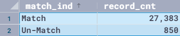
— Danilo

Field Notes: Orchestrating and Monitoring Complex, Long-running Workflows Using AWS Step Functions

Post Syndicated from Max Winter original https://aws.amazon.com/blogs/architecture/field-notes-orchestrating-and-monitoring-complex-long-running-workflows-using-aws-step-functions/

Situation:

IHS Markit’s Wall Street Office (WSO) offers financial reports to hundreds of clients worldwide. When IHS Markit completed the migration of WSO’s SaaS software to AWS, it unlocked the power and agility to deliver new product features monthly, as opposed to a multi-year release cycle. This migration also presented a great opportunity to further enhance the customer experience by automating the WSO reporting team’s own Continuous Integration and Continuous Deployment (CI/CD) workflow. WSO then offered the same migration workflow to its on-prem clients, who needed the ability to upgrade quickly in order to meet a regulatory LIBOR reporting deadline. This rapid upgrade was enabled by fully automating regression testing of new software versions.

In this blog post, I outline the architectures created in collaboration with WSO to orchestrate and monitor the complex, long-running reconciliation workflows in their environment by leveraging the power of AWS Step Functions. To enable each client’s migration to AWS, WSO needed to ensure that the new, AWS version of the reporting application produced identical outputs to the previous, on-premises version. For a single migration, the process is as follows:

  • spin up the old version of the SQL Server and reporting engine on Windows servers,
  • run reports,
  • repeat the process with the new version,
  • compare the outputs and review the differences.

The problem came with scaling this process.  IHS Markit provides financial solutions and tools to numerous clients. To enable these clients to transition away from LIBOR, the WSO team was tasked with migrating over 80 instances of the application, and reconciling hundreds of reports for each migration. During upgrades, customers must manually validate custom extracts created in the WSO Reporting application against current and next version, which limits upgrade frequency and increases the resourcing cost of these validations. Without automation, upgrading all clients would have taken an entire new Operations team, and cost the firm over 700 developer-hours to meet the regulatory LIBOR cessation deadline.

WSO was able to save over 4,000 developer-hours by making this process repeatable so it can be used as an automated regression test as part of the regular Systems Development Lifecycle process  The following diagram shows the reconciliation workflow steps enabled as part of this automated process.

Reconciliation Workflow Steps

Figure 1 – Reconciliation Workflow Steps

Complication:

The team quickly realized that a Serverless and event-driven solution would be required to make this process manageable. The initial approach was to use AWS Lambda functions to call PowerShell scripts to perform each step in the reconciliation process. They also used Amazon SNS to invoke the next Lambda function when the previous step completed.

The problem came when the Operations team tried to monitor these Lambda functions, with multiple parallel reconciliations running concurrently. The Lambda outputs became mixed together in shared Amazon Cloud Watch log groups, and there was no way to quickly see the overall progress of any given reconciliation workflow. It was also difficult to figure out how to recover from errors.

Furthermore, the team found that some steps in this process, such as database restoration, ran longer than the 15 minute Lambda timeout limit. As a result, they were forced to look for alternatives to manage these long-running steps. Following is an architecture diagram showing the serverless component used to automate and scale the process.

Initial Orchestration Architecture

Figure 2 – Initial Orchestration Architecture

Solution:

Enter Step Functions and AWS Systems Manager (formerly known as SSM) Automation. To address the problem of orchestrating the many sequential and parallel steps in our workflow, AWS Solutions Architects suggested replacing Amazon SNS with AWS Step Functions.

The Step Functions state machine controls the order in which the steps are invoked, including successful and error state transitions. The service is integrated with 14 other AWS services (Lambda function, SSM Automation, Amazon ECS, and more.), and can invoke them, as well as manual actions. These calls can be synchronous or run via steps that wait for an event. A state machine instance is long-lived and can support processes that take up to a year to complete.

Step Function Designer UI

Figure 3 – Step Function Designer UI

This immediately gave the Development team a holistic, visual way to design our workflow, and offered Operations a graphical user interface (UI) to monitor ongoing reconciliations in real time. The Step Functions console lists out all running and past reconciliations, including their status, and allows the operator to drill down into the detailed state diagram of any given reconciliation. The operator can then see how far it’s progressed or where it encountered an error.

The UI also provides Amazon CloudWatch links for any given step, isolating the logs of that particular Lambda execution, eliminating the need to search through the CloudWatch log group manually. The screenshot below illustrates what an in-progress Step Function looks to an operator, with each step listed out with its own status and a link to its log.

Step Function Execution Monitor

Figure 4 – Step Function Execution Monitor


Figure 5 - Step Function Execution Detail Viewer

Figure 5 – Step Function Execution Detail Viewer


Figure 6 -Step Function Log Group in CloudWatch

Figure 6 -Step Function Log Group in Amazon CloudWatch

The team also used the Step Function state machine as a container for metadata about each particular reconciliation process instance (like the environment ID and the database and Amazon EC2 instances associated with that environment), reducing the need to pass this data between Lambda functions.

To solve the problem of long-running PowerShell scripts, AWS Solutions Architects suggested using SSM Automation. Unlike Lambda functions, SSM Automation is meant to run operational scripts, with no maximum time limit. They also have native PowerShell integration, which you can use to call the existing scripts and capture their output.


SSM Automation UI for Monitoring Long-running Tasks and Manual Approval Steps

Figure 7 – SSM Automation UI for Monitoring Long-running Tasks and Manual Approval Steps

To save time running hundreds of reports, the team looked into the ‘Map State’ feature of Step Functions. Map takes an array of input data, then creates an instance of the step (in this case a Lambda call) for each item in this array.  It waits for them all to complete before proceeding.

This is recommended to implement as a fan-out pattern with almost no orchestration code. The Map State step also gives Operations users the option to limit the level of parallelism, in this case letting only 5 reports run simultaneously. This prevents overloading our reporting applications and databases.

Figure 8 – Map State is used to Fan Out the “CompareReport” Step as Multiple Parallel Steps

To deal with errors in any of the workflow steps, the Development team introduced a manual review step, which you can model in Step Functions. The manual step notifies a mailing list of the error, then waits for a reply to tell it whether to retry or abort the workflow.

The only challenge the Development team found was the mechanism for re-running an individual failed step. At this time, any failure needs to have an explicit state transition within the Step Function’s state diagram. While the Step Function can auto-retry a step, the team wanted to insert a wait-for-human-investigation step before retrying the more expensive and complex steps.

This presented 2 options:

  1. add wait-and-loop-back steps around every step we may want to retry,
  2. route all failures to a single wait-for-investigation step.

The former added significant complexity to the state machine, so AWS Solutions Architects raised this as a product feature that should be added to the Step Functions UI.

The proposed enhancement would allow any failed step to be manually rerun or skipped via UI controls, without adding explicit steps to each state machine to model this. In the meantime, the Dev team went with the latter approach, and had the human error review step loop back to the top of the state machine to retry the entire workflow. To avoid re-running long steps, they created a check within the step Lambda function to query the Step Functions API and determine whether that step had already succeeded before the loop-back, and complete it instantly if it had.


Human Intervention Steps Used to Allow Time to Review Results or Resolve Errors Before Retrying Failed Steps

Figure 9 – Human Intervention Steps Used to Allow Time to Review Results or Resolve Errors Before Retrying Failed Steps

Conclusion:

Within 6 weeks, WSO was able to run the first reconciliations and begin the LIBOR migration on time. The Step Function Designer instantly gave the Developer team an operator UI and workflow orchestration engine. Normally, this would have required the creation of an entire 3-tier stack, scheduler and logging infrastructure.

Instead, using Step Functions allowed the developers to spend their time on the reconciliation logic that makes their application unique. The report compare tool developed by the WSO team provides clients with automated artifacts confirming that customer report data remained identical between current version and next version of WSO. The new testing artifacts provide clients with robust and comprehensive testing of critical data extracts.

The Completed Step Function which Orchestrates an Entire Reconciliation Process

Figure 10 -The Completed Step Function which Orchestrates an Entire Reconciliation Process


We hope that this blog post provided useful insights to help determine if using AWS Step Functions are a good fit for you.

Field Notes provides hands-on technical guidance from AWS Solutions Architects, consultants, and technical account managers, based on their experiences in the field solving real-world business problems for customers.


Choosing a CI/CD approach: AWS Services with BigHat Biosciences

Post Syndicated from Mike Apted original https://aws.amazon.com/blogs/devops/choosing-ci-cd-aws-services-bighat-biosciences/

Founded in 2019, BigHat Biosciences’ mission is to improve human health by reimagining antibody discovery and engineering to create better antibodies faster. Their integrated computational + experimental approach speeds up antibody design and discovery by combining high-speed molecular characterization with machine learning technologies to guide the search for better antibodies. They apply these design capabilities to develop new generations of safer and more effective treatments for patients suffering from today’s most challenging diseases. Their platform, from wet lab robots to cloud-based data and logistics plane, is woven together with rapidly changing BigHat-proprietary software. BigHat uses continuous integration and continuous deployment (CI/CD) throughout their data engineering workflows and when training and evaluating their machine learning (ML) models.


BigHat Biosciences Logo


In a previous post, we discussed the key considerations when choosing a CI/CD approach. In this post, we explore BigHat’s decisions and motivations in adopting managed AWS CI/CD services. You may find that your organization has commonalities with BigHat and some of their insights may apply to you. Throughout the post, considerations are informed and choices are guided by the best practices in the AWS Well-Architected Framework.

How did BigHat decide what they needed?

Making decisions on appropriate (CI/CD) solutions requires understanding the characteristics of your organization, the environment you operate in, and your current priorities and goals.

“As a company designing therapeutics for patients rather than software, the role of technology at BigHat is to enable a radically better approach to develop therapeutic molecules,” says Eddie Abrams, VP of Engineering at BigHat. “We need to automate as much as possible. We need the speed, agility, reliability and reproducibility of fully automated infrastructure to enable our company to solve complex problems with maximum scientific rigor while integrating best in class data analysis. Our engineering-first approach supports that.”

BigHat possesses a unique insight to an unsolved problem. As an early stage startup, their core focus is optimizing the fully integrated platform that they built from the ground-up to guide the design for better molecules. They respond to feedback from partners and learn from their own internal experimentation. With each iteration, the quality of what they’re creating improves, and they gain greater insight and improved models to support the next iteration. More than anything, they need to be able to iterate rapidly. They don’t need any additional complexity that would distract from their mission. They need uncomplicated and enabling solutions.

They also have to take into consideration the regulatory requirements that apply to them as a company, the data they work with and its security requirements; and the market segment they compete in. Although they don’t control these factors, they can control how they respond to them, and they want to be able to respond quickly. It’s not only speed that matters in designing for security and compliance, but also visibility and track-ability. These often overlooked and critical considerations are instrumental in choosing a CI/CD strategy and platform.

“The ability to learn faster than your competitors may be the only sustainable competitive advantage,” says Cindy Alvarez in her book Lean Customer Development.

The tighter the feedback loop, the easier it is to make a change. Rapid iteration allows BigHat to easily build upon what works, and make adjustments as they identify avenues that won’t lead to success.

Feature set

CI/CD is applicable to more than just the traditional use case. It doesn’t have to be software delivered in a classic fashion. In the case of BigHat, they apply CI/CD in their data engineering workflows and in training their ML models. BigHat uses automated solutions in all aspects of their workflow. Automation further supports taking what they have created internally and enabling advances in antibody design and development for safer, more effective treatments of conditions.

“We see a broadening of the notion of what can come under CI/CD,” says Abrams. “We use automated solutions wherever possible including robotics to perform scaled assays. The goal in tightening the loop is to improve precision and speed, and reduce latency and lag time.”

BigHat reached the conclusion that they would adopt managed service offerings wherever possible, including in their CI/CD tooling and other automation initiatives.

“The phrase ‘undifferentiated heavy lifting’ has always resonated,” says Abrams. “Building, scaling, and operating core software and infrastructure are hard problems, but solving them isn’t itself a differentiating advantage for a therapeutics company. But whether we can automate that infrastructure, and how we can use that infrastructure at scale on a rock solid control plane to provide our custom solutions iteratively, reliably and efficiently absolutely does give us an edge. We need an end-to-end, complete infrastructure solution that doesn’t force us to integrate a patchwork of solutions ourselves. AWS provides exactly what we need in this regard.”

Reducing risk

Startups can be full of risk, with the upside being potential future reward. They face risk in finding the right problem, in finding a solution to that problem, and in finding a viable customer base to buy that solution.

A key priority for early stage startups is removing risk from as many areas of the business as possible. Any steps an early stage startup can take to remove risk without commensurately limiting reward makes them more viable. The more risk a startup can drive out of their hypothesis the more likely their success, in part because they’re more attractive to customers, employees, and investors alike. The more likely their product solves their problem, the more willing a customer is to give it a chance. Likewise, the more attractive they are to investors when compared to alternative startups with greater risk in reaching their next major milestone.

Adoption of managed services for CI/CD accomplishes this goal in several ways. The most important advantage remains speed. The core functionality required can be stood up very quickly, as it’s an existing service. Customers have a large body of reference examples and documentation available to demonstrate how to use that service. They also insulate teams from the need to configure and then operate the underlying infrastructure. The team remains focused on their differentiation and their core value proposition.


“We are automated right up to the organizational level and because of this, running those services ourselves represents operational risk,” says Abrams. “The largest day-to-day infrastructure risk to us is having the business stalled while something is not working. Do I want to operate these services, and focus my staff on that? There is no guarantee I can just throw more compute at a self-managed software service I’m running and make it scale effectively. There is no guarantee that if one datacenter is having a network or electrical problem that I can simply switch to another datacenter. I prefer AWS manages those scale and uptime problems.”

Embracing an opinionated model

BigHat is a startup with a singular focus on using ML to reduce the time and difficulty of designing antibodies and other therapeutic proteins. By adopting managed services, they have removed the burden of implementing and maintaining CI/CD systems.

Accepting the opinionated guardrails of the managed service approach allows, and to a degree reinforces, the focus on what makes a startup unique. Rather than being focused on performance tuning, making decisions on what OS version to use, or which of the myriad optional puzzle pieces to put together, they can use a well-integrated set of tools built to work with each other in a defined fashion.

The opinionated model means best practices are baked into the toolchain. Instead of hiring for specialized administration skills they’re hiring for specialized biotech skills.

“The only degrees of freedom I care about are the ones that improve our technologies and reduce the time, cost, and risk of bringing a therapeutic to market,” says Abrams. “We focus on exactly where we can gain operational advantages by simply adopting managed services that already embrace the Well-Architected Framework. If we had to tackle all of these engineering needs with limited resources, we would be spending into a solved problem. Before AWS, startups just didn’t do these sorts of things very well. Offloading this effort to a trusted partner is pretty liberating.”

Beyond the reduction in operational concerns, BigHat can also expect continuous improvement of that service over time to be delivered automatically by the provider. For their use case they will likely derive more benefit for less cost over time without any investment required.

Overview of solution

BigHat uses the following key services:


BigHat Reference Architecture

Security

Managed services are supported, owned and operated by the provider . This allows BigHat to leave concerns like patching and security of the underlying infrastructure and services to the provider. BigHat continues to maintain ownership in the shared responsibility model, but their scope of concern is significantly narrowed. The surface area the’re responsible for is reduced, helping to minimize risk. Choosing a partner with best in class observability, tracking, compliance and auditing tools is critical to any company that manages sensitive data.

Cost advantages

A startup must also make strategic decisions about where to deploy the capital they have raised from their investors. The vendor managed services bring a model focused on consumption, and allow the startup to make decisions about where they want to spend. This is often referred to as an operational expense (OpEx) model, in other words “pay as you go”, like a utility. This is in contrast to a large upfront investment in both time and capital to build these tools. The lack of need for extensive engineering efforts to stand up these tools, and continued investment to evolve them, acts as a form of capital expenditure (CapEx) avoidance. Startups can allocate their capital where it matters most for them.

“This is corporate-level changing stuff,” says Abrams. “We engage in a weekly leadership review of cost budgets. Operationally I can set the spending knob where I want it monthly, weekly or even daily, and avoid the risks involved in traditional capacity provisioning.”

The right tool for the right time

A key consideration for BigHat was the ability to extend the provider managed tools, where needed, to incorporate extended functionality from the ecosystem. This allows for additional functionality that isn’t covered by the core managed services, while maintaining a focus on their product development versus operating these tools.

Startups must also ask themselves what they need now, versus what they need in the future. As their needs change and grow, they can augment, extend, and replace the tools they have chosen to meet the new requirements. Starting with a vendor-managed service is not a one-way door; it’s an opportunity to defer investment in building and operating these capabilities yourself until that investment is justified. The time to value in using managed services initially doesn’t leave a startup with a sunk cost that limits future options.

“You have to think about the degree you want to adopt a hybrid model for the services you run. Today we aren’t running any software or services that require us to run our own compute instances. It’s very rare we run into something that is hard to do using just the services AWS already provides. Where our needs are not met, we can communicate them to AWS and we can choose to wait for them on their roadmap, which we have done in several cases, or we can elect to do it ourselves,” says Abrams. “This freedom to tweak and expand our service model at will is incomparably liberating.”

Conclusion

BigHat Biosciences was able to make an informed decision by considering the priorities of the business at this stage of its lifecycle. They adopted and embraced opinionated and service provider-managed tooling, which allowed them to inherit a largely best practice set of technology and practices, de-risk their operations, and focus on product velocity and customer feedback. This maintains future flexibility, which delivers significantly more value to the business in its current stage.

“We believe that the underlying engineering, the underlying automation story, is an advantage that applies to every aspect of what we do for our customers,” says Abrams. “By taking those advantages into every aspect of the business, we deliver on operations in a way that provides a competitive advantage a lot of other companies miss by not thinking about it this way.”

About the authors

Mike is a Principal Solutions Architect with the Startup Team at Amazon Web Services. He is a former founder, current mentor, and enjoys helping startups live their best cloud life.


Sean is a Senior Startup Solutions Architect at AWS. Before AWS, he was Director of Scientific Computing at the Howard Hughes Medical Institute.

Building an ARM64 Rust development environment using AWS Graviton2 and AWS CDK

Post Syndicated from Alistair McLean original https://aws.amazon.com/blogs/devops/building-an-arm64-rust-development-environment-using-aws-graviton2-and-aws-cdk/

2020 was the year that ARM chips made the headlines by moving from largely mobile form factors into the cloud thanks to AWS Graviton2, allowing you to have up to 40% better price performance over comparable current generation x86 Amazon Elastic Compute Cloud (Amazon EC2) and Amazon Relational Database Service (Amazon RDS) instances.

We speak to customers daily about Graviton2. One recurring question we hear is “Graviton2 is great, but how can my team develop for ARM natively without the complexity of cross-compilation or having to buy custom hardware on premises?” This post seeks to answer that question by setting up the Visual Studio Code-based Code Server IDE, running on a Graviton2 EC2 instance that enables native development in a cost-effective and secure manner accessed via your browser.

The Rust programming language has gained a huge amount of popularity recently. This post aims to show that you can use this environment for Rust development as well as hundreds of other supported languages. AWS has committed to supporting the Rust community and using the language to deliver fast and robust services to customers at scale, and we want to enable our customers to do the same.

We also include instructions for building and installing the rust-analyzer and CodeLLDB debugger plugins to add additional language features.

Solution overview

The following diagram illustrates our solution architecture.

Architecture of the solution showing components and their linkages

The solution consists of an EC2 Graviton2 instance located in a private VPC subnet routed through an AWS Global Accelerator accelerator to provide routing optimization and keep packet loss, jitter, and latency lower by up to 60%. An internal facing Application Load Balancer containing the AWS Certificate Manager certificate decrypts and forwards traffic to this instance.

Code Server queries AWS Secrets Manager to initially set the login password on startup and allow for continued password-based authentication and easy password rotation. The EC2 instance has access to the internet through a NAT gateway and has no public IP address or key pair associated, and is accessible only through AWS Systems Manager Session Manager.

Prerequisites

For this walkthrough, the following are prerequisites:

AWS CDK stack

In order to deploy our architecture, I use the AWS CDK. As a developer, it’s more intuitive to me to define my infrastructure using a language and tooling with which I am familiar. I can also do things like environment variable injection and scripting as part of the stack creation to add stack parameters and customization points.

The AWS CDK application is comprised of five stacks. Each stack defines a separate part of the architecture:

  • Networking – Defines a VPC across two Availability Zones with the CIDR range of your choice. The routing and public/private subnet creation is done for us as part of the default configuration.

  • Certificate – This is the reason for the domain prerequisite. It’s a best practice to encrypt web applications using TLS, and for that we need a certificate and therefore a domain. This stack creates a certificate for the subdomain you specify as part of the stack creation and DNS validation in Route 53.
  • Amazon EC2 configuration – This defines both our AMI and the instance type and configuration. In this case, we’re using Amazon Linux 2 ARM64 edition. Here we also set the instance-managed roles that allow Session Manager connectivity and Secrets Manager access.
  • ALB configuration – Here we define the internal load balancer and specify the listener, certificate, and target configuration. I have injected the Amazon EC2 configuration as part of the class constructor so that I can reference it directly as a target.
  • Global accelerator configuration – Finally, the accelerator is defined here with two ports open, the ALB we defined in the ALB stack as a target, and most importantly adds in a CNAME DNS entry pointing to the DNS name of the accelerator.

Walkthrough overview

This walkthrough uses the AWS CDK command line tools to deploy the stack. Session Manager is enabled to allow access to the EC2 instance and configure the Code Server application and associated plugins.

The walkthrough specifically covers the following steps:

  1. Deploy the AWS CDK stacks via CloudShell to build out the application infrastructure and associated IAM roles.
  2. Launch Code Server via the official Docker container with the commands to get and set the password stored in Secrets Manager.
  3. Log in and build the rust-analyzer and CodeLLDB plugins from a terminal to allow for debugging within a “Hello World” application.

Start CloudShell and install the appropriate tooling

In this section, I use dummy values for the domain, the VPC CIDR, AWS Region, and the secret password. You need to submit real values as appropriate.

Sign in to CloudShell and enter the following commands:

sudo yum groupinstall -y "Development Tools"
sudo npm install aws-cdk -g
git clone https://github.com/aws-samples/cdk-graviton2-alb-aga-route53.git
cd cdk-graviton2-alb-aga-route53
python3 -m venv .
source bin/activate
python -m pip install -r requirements.txt
export VPC_CIDR=”10.0.0.1/16” #Substitute your CIDR here.
export CDK_DEPLOY_ACCOUNT=`aws sts get-caller-identity | jq -r '.Account'`
export CDK_DEPLOY_REGION=$AWS_REGION
export R53_DOMAIN=”code-server.example.com” #Substitute your domain here.
cdk bootstrap aws://$CDK_DEPLOY_ACCOUNT/$CDK_DEPLOY_REGION
cdk deploy --all

The deploy step takes around 10-15 mins to run and prompts a couple of times to add resources like security groups and IAM roles.

Log in to the new instance using Session Manager

Install the latest version of the Session Manager plugin for the AWS CLI:

cd ~
curl "https://s3.amazonaws.com/session-manager-downloads/plugin/latest/linux_64bit/session-manager-plugin.rpm" -o "session-manager-plugin.rpm"
sudo yum install -y session-manager-plugin.rpm

Now start a session, logging into the newly created EC2 instance and log in as ec2-user:

aws ssm start-session --target i-1234xyz7890abc #Substitute the instance id we just created here
#Once session is active:
sudo su - ec2-user

Add the password as a secret and start the container

Enter the following code to add the password as a secret in Secrets Manager and start the container:

aws secretsmanager create-secret --name CodeServerProd --secret-string Password123abc # Substitute the appropriate password here.
sudo docker run -d --name=code-server -e PUID=1000 -e PGID=1000 -e PASSWORD=`aws secretsmanager get-secret-value --secret-id CodeServerProd | jq -r '.SecretString'` -p 8080:8080 -v /home/ec2-user/.config:/config --restart unless-stopped codercom/code-server

Access and configure the web application for Rust development

So far, we have accomplished the following:

  • Created the infrastructure in the diagram via AWS CDK deployment
  • Configured the EC2 instance to run Docker and added this to the systemctl startup scripts
  • Created a secret in Secrets Manager to use as the application login password
  • Instantiated a Docker container running Code Server

Next, we access the running container via the web interface and install the required development tools.

Log in to the Code Server web application

To log in to the Code Server web application, complete the following steps:

  1. Browse to https://code-server.example.com, where example.com is the name of the domain you supplied in the AWS CDK step.
  2. Log in using the password you created in Secrets Manager.
  3. Create a new terminal by choosing the hamburger icon and, under Terminal, choosing New Terminal.
  4. Issue the following commands into the terminal to install the Rust programming language:
bash
sudo apt update && sudo apt upgrade -y
sudo apt install -y build-essential npm clang lldb
curl --proto '=https' --tlsv1.2 -sSf https://sh.rustup.rs | sh
source $HOME/.cargo/env

Install the rust-analyzer plugin

Open the extensions panel and enter Rust Analyzer in the search bar. Then install the plugin.

Install the debugger

Go back to the extensions panel in the Code Server application and enter CodeLLDB into the search bar. Then install this extension.

Create a sample application and open it in the Code Server window

To create and use our sample application, complete the following steps:

  • In the existing Code Server terminal, enter the following:
mkdir -p ~/src/
cd ~/src
cargo new helloworld --bin
  • Open the newly created folder in Code Server verifying that the helloworld directory was successfully created.

Open File or Folder dialog in Code Server

  • Rust-analyzer runs when you open up src/main.rs and index the file.
  • You can run the program by choosing Run in the editor.

Main Code Server editor window showing helloworld Rust program code.

  • Similarly, to launch the debugger, choose Debug in the editor.

Code Server Debugger view

Troubleshooting

If the CloudShell session times out, you need to reset your environment variables in order to re-deploy, modify, and delete the stack deployment.

Clean up

This stack incurs an estimated monthly cost of $143.00.

To delete the stack, log in to CloudShell and enter the following commands:

cd cdk-graviton2-alb-aga-route53
source bin/activate

# Re-set the environment variables again if required
export VPC_CIDR=”10.0.0.1/16” #Substitute your CIDR here.
export CDK_DEPLOY_ACCOUNT=`aws sts get-caller-identity | jq -r '.Account'`
export CDK_DEPLOY_REGION=$AWS_REGION
export R53_DOMAIN=”code-server.example.com” #Substitute your domain here.
cdk destroy --all

This destroys all the resources created in the first step. You can verify this by browsing to the AWS CloudFormation console and noting the deletion of all the stacks.

Conclusion

AWS is a place where builders can reinvent the future. The future of development means supporting different chipsets depending on different business requirements. This post is designed to enable development targeting the ARM64 microarchitecture by utilizing AWS Graviton2. Happy building!

Author bio

Author portrait

Alistair is a Principal Solutions Architect at AWS focused on EdTech customers. Originally from the west coast of Scotland, Alistair now lives in Fairfield, Connecticut, with his wife and two daughters and enjoys spending time with his family, skiing, golfing, cycling, and using his pellet smoker.

How Amazon CodeGuru Profiler helps Coursera create high-quality online learning experiences

Post Syndicated from Adnan Bilwani original https://aws.amazon.com/blogs/devops/coursera-codeguru-profiler/

This guest post was authored by Rana Ahsan and Chris Liu, Software Engineers at Coursera, and edited by Dave Sanderson and Adnan Bilwani, at AWS.

Coursera was launched in 2012 by two Stanford Computer Science professors, Daphne Koller and Andrew Ng, with a vision of providing universal access to world-class learning. It’s now one of the world’s leading online learning platforms with more than 77 million registered learners. Coursera partners with over 200 leading university and industry partners to offer a broad catalog of content and credentials, including Guided Projects, courses, Specializations, certificates, and accredited bachelor’s and master’s degrees. More than 6,000 institutions have used Coursera to transform their talent by upskilling and reskilling their employees, citizens, and students in the high-demand data science, technology, and business skills required to compete in today’s economy.

Coursera’s challenge

About a year and a half ago, we were debugging some performance bottlenecks for our microservices where some requests were too slow and often resulted in server errors due to timeout. Even after digging into the logs and looking through existing performance metrics of the underlying systems, we couldn’t determine the cause or explain the behavior. To compound the matter, we saw the issues across multiple applications, leading to a concern that the issue resided in code shared across applications.

To dig deeper into the problem, we started doing manual reviews of the code for the applications associated with these failures. This process turned out to be too laborious and time-consuming.

We also started building out our debugging solution utilizing shell scripts to capture a snapshot of the system and application state so we could analyze the details of these bottlenecks. Although the scripts provided some valuable insights, we started to run into issues of scale. The process of deploying the tooling and collecting the data became tedious and cumbersome. At the same time, the more data we received back from our scripts, the more demand we saw for this level of detail.

Solution with Amazon CodeGuru

It was at this point we decided to look into CodeGuru Profiler to determine if it could provide the same insights as our tooling while reducing the administrative burden associated with deploying, aggregating, and analyzing the data.

Quickly after deploying CodeGuru Profiler, we started to get valuable and actionable data regarding the issue. The profiler highlighted a high CPU usage during the deserialization process used for application communications (see the following screenshot). This confirmed our suspicions that the issue was indeed in the shared code, but it was also an unexpected find, because JSON deserialization is widespread and it hadn’t hit our radar as a potential candidate for the issue.

Flame graph highlighted high CPU usage

The deserialization performance was causing slow processing time for each request and increasing the overall communication latency. This led to performance degradation by causing the calls to slowly stack up over time until the request would time out. With CodeGuru Profiler, we were also able to establish a relationship between the size of the JSON document and the high CPU usage. As the document size increased, so did CPU usage. In some cases, this resulted in a resource starvation situation on the system, which in turn could cause other processes on the instance to crash, resulting in a sudden failure.

In addition to the performance and application instances failures, the high CPU usage during deserialization was quietly driving up costs. Because the issue was in shared code, the wasteful resource consumption was contributing to the need for additional instances to be added into the application cluster in order to meet throughput requirements.

Results

The details from CodeGuru Profiler enabled us to see and understand the underlying cause and move forward with a solution. Because the code is in the critical communication path for our microservices and shared across many applications, we decided to replace the JSON serialization with an alternative object serialization approach that was much more performant.

To get a deeper understanding of the performance impact of this change, we deployed the original code to a test environment. We used CodeGuru Profiler to evaluate the performance of the JSON and native object serialization. After we ran the same battery of tests against the new code, the deserialization CPU usage dropped between 30–40%.

Flame graph displayed lower CPU usage after changes

This resulted in a corresponding decrease in serialization-deserialization latency of 5–50% depending on response payload size and workload.

As we roll out this optimization across our fleet, we anticipate seeing significant improvements in the performance and stability of our microservices platform as well as a reduction in CPU utilization cost.

Conclusion

CodeGuru Profiler provides additional application insights and helps us troubleshoot other issues in our applications, including resolving a case of flaky I/O errors and improving tail latency by recommending a different thread-pooling strategy.

CodeGuru Profiler was easy to maintain and scale across our fleet. It quickly identified these performance issues in our production environment and helped us verify and understand the impact of possible resolutions prior to releasing the code back into production.


About the authors

Rana Ahsan is a Staff Software Engineer at Coursera
Chris Liu is a Staff Software Engineer at Coursera
Adnan Bilwani is a Sr. Specialist Builders Experience at AWS
Dave Sanderson is a Sr. Technical Account Manager at AWS


Integrate GitHub monorepo with AWS CodePipeline to run project-specific CI/CD pipelines

Post Syndicated from Vivek Kumar original https://aws.amazon.com/blogs/devops/integrate-github-monorepo-with-aws-codepipeline-to-run-project-specific-ci-cd-pipelines/

AWS CodePipeline is a continuous delivery service that enables you to model, visualize, and automate the steps required to release your software. With CodePipeline, you model the full release process for building your code, deploying to pre-production environments, testing your application, and releasing it to production. CodePipeline then builds, tests, and deploys your application according to the defined workflow either in manual mode or automatically every time a code change occurs. A lot of organizations use GitHub as their source code repository. Some organizations choose to embed multiple applications or services in a single GitHub repository separated by folders. This method of organizing your source code in a repository is called a monorepo.

This post demonstrates how to customize GitHub events that invoke a monorepo service-specific pipeline by reading the GitHub event payload using AWS Lambda.


Solution overview

With the default setup in CodePipeline, a release pipeline is invoked whenever a change in the source code repository is detected. When using GitHub as the source for a pipeline, CodePipeline uses a webhook to detect changes in a remote branch and starts the pipeline. When using a monorepo style project with GitHub, it doesn’t matter which folder in the repository you change the code, CodePipeline gets an event at the repository level. If you have a continuous integration and continuous deployment (CI/CD) pipeline for each of the applications and services in a repository, all pipelines detect the change in any of the folders every time. The following diagram illustrates this scenario.


GitHub monorepo folder structure


This post demonstrates how to customize GitHub events that invoke a monorepo service-specific pipeline by reading the GitHub event payload using Lambda. This solution has the following benefits:

  • Add customizations to start pipelines based on external factors – You can use custom code to evaluate whether a pipeline should be triggered. This allows for further customization beyond polling a source repository or relying on a push event. For example, you can create custom logic to automatically reschedule deployments on holidays to the next available workday.
  • Have multiple pipelines with a single source – You can trigger selected pipelines when multiple pipelines are listening to a single GitHub repository. This lets you group small and highly related but independently shipped artifacts such as small microservices without creating thousands of GitHub repos.
  • Avoid reacting to unimportant files – You can avoid triggering a pipeline when changing files that don’t affect the application functionality (such as documentation, readme, PDF, and .gitignore files).

In this post, we’re not debating the advantages or disadvantages of a monorepo versus a single repo, or when to create monorepos or single repos for each application or project.


Sample architecture

This post focuses on controlling running pipelines in CodePipeline. CodePipeline can have multiple stages like test, approval, and deploy. Our sample architecture considers a simple pipeline with two stages: source and build.


Github monorepo - CodePipeline Sample Architecture

This solution is made up of following parts:

  • An Amazon API Gateway endpoint (3) is backed by a Lambda function (5) to receive and authenticate GitHub webhook push events (2)
  • The same function evaluates incoming GitHub push events and starts the pipeline on a match
  • An Amazon Simple Storage Service (Amazon S3) bucket (4) stores the CodePipeline-specific configuration files
  • The pipeline contains a build stage with AWS CodeBuild


Normally, after you create a CI/CD pipeline, it automatically triggers a pipeline to release the latest version of your source code. From then on, every time you make a change in your source code, the pipeline is triggered. You can also manually run the last revision through a pipeline by choosing Release change on the CodePipeline console. This architecture uses the manual mode to run the pipeline. GitHub push events and branch changes are evaluated by the Lambda function to avoid commits that change unimportant files from starting the pipeline.


Creating an API Gateway endpoint

We need a single API Gateway endpoint backed by a Lambda function with the responsibility of authenticating and validating incoming requests from GitHub. You can authenticate requests using HMAC security or GitHub Apps. API Gateway only needs one POST method to consume GitHub push events, as shown in the following screenshot.


Creating an API Gateway endpoint


Creating the Lambda function

This Lambda function is responsible for authenticating and evaluating the GitHub events. As part of the evaluation process, the function can parse through the GitHub events payload, determine which files are changed, added, or deleted, and perform the appropriate action:

  • Start a single pipeline, depending on which folder is changed in GitHub
  • Start multiple pipelines
  • Ignore the changes if non-relevant files are changed

You can store the project configuration details in Amazon S3. Lambda can read this configuration to decide what needs to be done when a particular folder is matched from a GitHub event. The following code is an example configuration:

{

    "GitHubRepo": "SampleRepo",

    "GitHubBranch": "main",

    "ChangeMatchExpressions": "ProjectA/.*",

    "IgnoreFiles": "*.pdf;*.md",

    "CodePipelineName": "ProjectA - CodePipeline"

}

For more complex use cases, you can store the configuration file in Amazon DynamoDB.

The following is the sample Lambda function code in Python 3.7 using Boto3:

def lambda_handler(event, context):

    import json
    modifiedFiles = event["commits"][0]["modified"]
    #full path
    for filePath in modifiedFiles:
        # Extract folder name
        folderName = (filePath[:filePath.find("/")])
        break

    #start the pipeline
    if len(folderName)>0:
        # Codepipeline name is foldername-job. 
        # We can read the configuration from S3 as well. 
        returnCode = start_code_pipeline(folderName + '-job')

    return {
        'statusCode': 200,
        'body': json.dumps('Modified project in repo:' + folderName)
    }
    

def start_code_pipeline(pipelineName):
    client = codepipeline_client()
    response = client.start_pipeline_execution(name=pipelineName)
    return True

cpclient = None
def codepipeline_client():
    import boto3
    global cpclient
    if not cpclient:
        cpclient = boto3.client('codepipeline')
    return cpclient
   

Creating a GitHub webhook

GitHub provides webhooks to allow external services to be notified on certain events. For this use case, we create a webhook for a push event. This generates a POST request to the URL (API Gateway URL) specified for any files committed and pushed to the repository. The following screenshot shows our webhook configuration.

Creating a GitHub webhook2

Conclusion

In our sample architecture, two pipelines monitor the same GitHub source code repository. A Lambda function decides which pipeline to run based on the GitHub events. The same function can have logic to ignore unimportant files, for example any readme or PDF files.

Using API Gateway, Lambda, and Amazon S3 in combination serves as a general example to introduce custom logic to invoke pipelines. You can expand this solution for increasingly complex processing logic.


About the Author

Vivek Kumar

Vivek is a Solutions Architect at AWS based out of New York. He works with customers providing technical assistance and architectural guidance on various AWS services. He brings more than 23 years of experience in software engineering and architecture roles for various large-scale enterprises.


Gaurav-Sharma

Gaurav is a Solutions Architect at AWS. He works with digital native business customers providing architectural guidance on AWS services.


Nitin-Aggarwal

Nitin is a Solutions Architect at AWS. He works with digital native business customers providing architectural guidance on AWS services.


Field Notes: How FactSet Uses ‘microAccounts’ to Reduce Developer Friction and Maintain Security at Scale

Post Syndicated from Tarik Makota original https://aws.amazon.com/blogs/architecture/field-notes-how-factset-uses-microaccounts-to-reduce-developer-friction-and-maintain-security-at-scale/

This is post was co-written by FactSet’s Cloud Infrastructure team, Gaurav Jain, Nathan Goodman, Geoff Wang, Daniel Cordes, Sunu Joseph and AWS Solution Architects, Amit Borulkar and Tarik Makota.

FactSet considers developer self-service and DevOps essential for realizing cloud benefits.  As part of their cloud adoption journey, they wanted developers to have a frictionless infrastructure provisioning experience while maintaining standardization and security of their cloud environment.  To achieve their objectives, they use what they refer to as a ‘microAccounts approach’. In their microAccount approach, each AWS account is allocated for one project and is owned by a single team.

In this blog, we describe how FactSet manages 1000+ AWS accounts at scale using the microAccounts approach. First, we cover the core concepts of their approach. Then we outline how they manage access and permissions. Finally, we show how they manage their networking implementation and how they use automation to manage their AWS Cloud infrastructure.

How FactSet started with AWS

They started their cloud adoption journey with what they now call a ‘macroAccounts’ approach. In the early days they would set up a handful of AWS accounts. These macroAccounts were then shared across several different application teams and projects.   They have hundreds of application teams along with thousands of developers and they quickly experienced the challenges of a macroAccounts approach. These include the following:

  1. AWS Identity and Access Management (IAM) policies and resource tagging were complex to design in order to maintain least privilege. For example, if a developer desired the ability to start/stop Amazon EC2 instances, they would need to ensure that they are limited to starting/stopping only their own instances.  This complexity kept increasing as developers wanted to automate their workflows using constructs such as AWS Lambda functions, and containers.
  2. They had difficulty in properly attributing cloud costs across departments.  More importantly they kept going back and forth on: how do we establish accountability and transparency around spends by groups, projects, or teams?
  3. It was difficult to track and manage impact of infrastructure change to FactSet applications. For example, how is maintenance off underlying security group or IAM policy affecting FactSet applications?
  4. Significant effort was required in managing service quotas and limits across various applications being under single AWS account.

FactSet’s solution – microAccounts

Recognizing the issues, they decided to take a different approach to AWS account management. Instead of creating a few shared macro-accounts, they decided to create one AWS account per project (microAccounts) with clearly defined ownership and product allocation.  An analogy might be that macro-accounts were like leaving the main door of a house open but locking individual closets and rooms to limit access. This is opposed to safeguarding the entry to the house but largely leaving individual closets and rooms open for the tenant to manage.

Benefits of microAccounts

They have been operating their AWS Cloud infrastructure using microAccounts for about two years now. Benefits of the microAccount approach include:

1.      Access & Permissions: By associating an account with a project they simplified which services are allowed, which resources that development team can access, and are able to ensure that those permissions cascade properly to underlying resources.  The following diagram shows their microAccount strategy.


Tagging versus microAccount strategy

Figure 1 – Tagging versus microAccount strategy

2.      Service Quotas & Limits: Given most service quotas are account specific, microAccounts allow their developers to plan limits based on their application needs.  In a shared account configuration, there was no mechanism to limit separate teams from using up a larger portion of the service quota, leaving other teams with less.  These limits extend beyond infrastructure provisioning to run time tasks like Lambda concurrency, API throttling limits on parameter store and more.

3.      AWS Service Permissions: microAccounts allowed FactSet to easily implement least privilege across services. By using IAM service control policies (SCPs) they limit what AWS services an account can access.  They start with a default set of services and based on business need we can grant a specific account access to other non-common services without having to worry about those services creeping into other use cases.  For example, they disable storage gateway by default, but can allow access for a specific account if needed.

4.      Blast Radius Containment:  microAccounts provides the ability to create safety boundaries. This is in the event of any stability and security issues, they stay isolated within that specific application (AWS account) and they don’t affect operations of other applications.

5.     Cost Attributions:  Clearly defined account ownership provides a simple and straightforward way to attribute costs to a specific team, project, or product.  They don’t have to enforce the tagging individual resources for cost purposes. AWS account acts like an application resource group so all resources in the account are implicitly tagged.

6.      Account Notifications & Operations:  Single threaded account ownership allows FactSet to automatically relay any required notification to right developers.  Moreover, given that account ownership is fundamental in defining who is allowed access to the account, there is a high level of confidence in the validity of this mapping as opposed to relying on just tagging.

7.      Account Standards & Extensions: we manage microAccounts through a CI/CD pipeline which allows us to standardize and extend without interruptions.  For example, all their microAccounts are provisioned with a standard AWS Key Management Service (AWS KMS) key, an AWS Backup Vault & policy, private Amazon Route 53 zone, AWS Systems Manager Parameter Store with network information for Terraform or AWS CloudFormation templates.

8.      Developer Experience: microAccount automation and guardrails allow developers to get started quickly instead of spending time debugging things like correct SCP/IAM permissions and more. Developers tend to work across multiple applications and their experience has improved as they have a standard set of expectations for their AWS environment. This is particularly useful as they move from application to application.

Access and permissions for microAccounts

FactSet creates every AWS account with a standard set of IAM roles and permissions. Furthermore, each account has its own SCP which defines the list of services allowed in the account.  Based on application needs, they can extend the permissions.  Interactive roles are mapped to an ActiveDirectory (AD) group, and membership of the AD group is managed by the development teams themselves.  Standard roles are:

  • DevOps Role – Interactive role used to provision and manage infrastructure.
  • Developer Role – Interactive role used to read/write data (and some infrastructure)
  • ReadOnly Role – Interactive role with read-only access to the account.  This can be granted to account supervisors, product developers, and other similar roles.
  • Support Roles – Interactive roles for certain admin teams to assist account owners if needed
  • ServiceExecutionRole – Role that can be attached to entities such as Lambda functions, CodeBuild, EC2 instances, and has similar permissions to a developer role.
IAM Role Privileges

Figure 2 – IAM Role Privileges

Networking for microAccounts

  • FactSet leverages AWS Resource Access Manager (RAM) to share appropriate subnets with each account.  Each microAccount provisioned has access to subnets by sing AWS Shared VPCs.  They create a single VPC per business unit per environment (Dev, Prod, UAT, and Shared Services) in each region.  RAM enabled them to easily and securely share AWS resources with any AWS account within their AWS Organization.  When an account is created they allocate appropriate subnets to that account.
  • They use AWS Transit Gateway to manage inter-VPC routing and communication across multiple VPCs in a region.  They didn’t want to limit our ability to scale up quickly.  AWS Transit Gateway is a single place to land their AWS Direct Connect circuits in each Region.  It provides them with a consolidated place to manage routing tables that propagated to each VPC when they are attached.


VPC Sharing for microAccounts

Figure 3 – VPC Sharing for microAccounts

Automation & Config Management for microAccounts

To create frictionless self-service cloud infrastructure early on, FactSet realized that automation is a must.  Their infrastructure automation uses source-control as a source of truth for defining each microAccount. This helps them ensure repeatable and standardized account provisioning process, as well as flexibility to adjust specific settings and permissions on per account needs.

Account provisioning flow

Figure 4 – Account provisioning flow

By default, their accounts are only enabled in a small set of Regions.  They control it via the following policy block.  If they add new Region(s), they would implement that change in source-control and automated enforcement checks would add it to SCP.

{
    "Sid": "DenyOtherRegions",
    "Effect": "Deny",
    "Action": "*",
    "Resource": "*",
    "Condition": {
        "StringNotEquals": {
            "aws:RequestedRegion": ["us-east-1","eu-west-2"]
        },
        "ForAllValues:StringNotLike": {
            "aws:PrincipalArn": [
                "arn:aws:iam::*:role/cloud-admin-role"
    }
}

Lessons Learned

During their journey to adopt microAccounts, FactSet came across some new challenges that are worth highlighting:

  1. IAM role creation: Their DevOps Role can create new IAM roles within the account.  To ensure that newly created role complies with least-privilege principles, they attach a standard permission boundary which limits its permissions to not extend beyond DevOps level.
  2. Account Deletion: While AWS provides APIs for account creation, currently there is no API to delete or rename an account.  This is not an issue since only a small percentage of accounts had to be deleted because of a cancelled project for example.
  3. Account Creation / Service Activation: Although automation is used to provision accounts it can still take time for all services in account to be fully activated.  Some services like Amazon EC2 have asynchronous processes to be activated in a new account.
  4. Account Email, Root Password, and MFA: Upon account creation, they don’t set up a root password or MFA.  That is only setup on the primary (master) account.  Given each account requires a unique email address, they leverage Amazon Simple Email Service (Amazon SES) to create a new email address with cloud administrator team as the recipients.  When they need to log in as root (very unusual), they go through the process of password reset before logging in.
  5. Service Control Policies: There were two primary challenges related to SCPs:
    • SCP is a property in the primary (master) account that is attached to a child microAccount.  However, they also wanted to manage SCP like any other account config and store it in source-control along with other account configuration.  This required IAM role used by our automation to have special permissions to be able to create/attach/detach SCPs in the primary (master) account.
    • There is a hard limit of 1000 SCPs in the primary (master) account.  If you have a SCP per account, this would limit you to 1000 microAccounts.  They solved this by re-using SCPs across accounts with same policies.  Content of a policy is hashed to create a unique SCP identifier, and accounts with same hashes are attached to same SCP.
  6. Sharing data (typically S3) across microAccounts: they leverage a concept of “trusted-accounts” to allow other accounts access to an account’s resources including S3 and KMS keys.
  7. It may feel like an anti-pattern to have resources with static costs like Application Load Balancers (ALB) and KMS for individual projects as opposed to a shared pool.  The list of resources with a base cost is small as most of the services are largely priced based on usage.  For FactSet, resource isolation is a key benefit of microAccounts, and therefore outweighs some of these added costs.
  8. Central Inventory & Logging: With 100s of accounts, it is worth investing in a more centralized inventory and AWS CloudTrail logs collection system.
  9. Costs, Reserved Instances (RI), and Savings Plans: FactSet found AWS Cost Explorer at the level of your primary (master) account to be a great tool for cost-transparency.  They leverage AWS Cost Explorer’s API to import that data into their internal cost transparency tools.  RIs and Savings Plans are managed centrally and leverage automatic sharing between accounts within the same master (primary) organization.

Conclusion

The microAccounts approach provides FactSet with the agility to operate according to specific needs of different teams and projects in the enterprise. They are currently deploying in twelve AWS Regions with automated AWS account provisioning happening in minutes and drift checks executing multiple times throughout the day. This frees up their developers to focus on solving business problems to maximize the benefits of cloud computing, so that their business can innovate and accelerate their clients’ digital transformations.

Their experience operating regulated infrastructure in the cloud demonstrated that microAccounts are pivotal for managing cloud at scale. With microAccounts they were able to accelerate projects onboarded to cloud by 5X, reduce number of IAM permission tickets by 10X, and experienced 3X fewer stability issues. We hope that this blog post provided useful insights to help determine if the microAccount strategy is a good fit for you.

In their own words, FactSet creates flexible, open data and software solutions for tens of thousands of investment professionals around the world, which provides instant access to financial data and analytics that investors use to make crucial decisions. At FactSet, we are always working to improve the value that our products provide.

Recommended Reading:

Defining an AWS Multi-Account Strategy for telecommunications companies

Why should I set up a multi-account AWS environment?

Field Notes provides hands-on technical guidance from AWS Solutions Architects, consultants, and technical account managers, based on their experiences in the field solving real-world business problems for customers.