Over the past five years, we’ve made lots of online educational video content for our online courses, for our Isaac Computer Science platform for GCSE and A level, and for our remote lessons based on our Teach Computing Curriculum hosted on Oak National Academy.

We have learned a lot from experience and from learner feedback, and we want to share this knowledge with others. We’re also aware there’s always more to learn from people across the computing education community. That’s one reason we’re continually working to broaden the range of educators we work with. Another is that we want all learners to see themselves represented in our educational materials, because everyone belongs in computer science.

Facilitators and participants involved in the Teach Online programme. — RPF staff and the Teach Online participants

To make progress with all these goals, we ran a pilot programme for educators called Teach Online at the end of 2021 and the start of 2022. Through Teach Online, we provided twelve educators with training, opportunities, and financial and material support to help them with creating online educational content, particularly videos.

Over five online sessions and a final in-person day, we trained them in not only the production of educational videos, but also some of the pedagogy behind it. The pilot programme has now finished, and we thought we’d share some of the key points from the sessions with you in the wider community.

Learning to create a great online learning experience

When you learn new skills and knowledge, it’s important to think about how you apply these. For this reason, a useful question you can use throughout the learning process is “Why?”. So as you think about how to create the best online learning experience, ask yourself in different contexts throughout the content design and production:

Why am I using this style of video to illustrate this topic?
Why am I presenting these ideas in this order?
Why am I using this choice of words?

For example, it’s easy to default to creating ‘talking head’ videos featuring one person talking directly to the camera. But you should always ask why — what are the reasons for using a ‘talking head’ style. Instead, or in addition, you can make videos more engaging and support the learning experience by:

Turning the video into an interview
Adding other camera angles or screencasts to focus on demonstrations
Cutting away to B-roll footage (additional video that can provide context or related action, while the voiceover continues) or to still images that help connect a concept to concrete examples

Teach Computing programme participant. — Teach Online participants explored different ways to make their videos engaging

Planning is key

By planning your content carefully instead of jumping into production right away, you can:

Better visualise what your video should look like by creating a storyboard
Keep learners engaged by deliberately splitting learning up into smaller chunks while still keeping a narrative flow between them
Develop your learners’ understanding of key computing concepts by using semantic waves to unpack and repack concepts

The Teach Online participants told us that they particularly enjoyed learning more about planning videos:

“I now understand that a little planning can make the difference between a mediocre online learning experience and a professional-looking valuable learning experience.” – Educator who participated in our Teach Online programme

“Planning the session using a storyboard is so helpful to visualise the actual recording.” – Educator who participated in our Teach Online programme

Storyboard from a Teach Computing participant. — Storyboards are a great option to plan online learning experiences

Considering equity, diversity, and inclusion

We are committed to making computing and computer science accessible and engaging, so we embed measures to improve equity, diversity, and inclusion throughout our free learning and teaching resources, including the Teach Online programme. It’s important not to leave this aspect of creating educational content as an afterthought: you can only make sure that your content is truly as equitable and inclusive as you can make it if you address this at every stage of your process. As an added bonus, many ways of making your content more accessible not only benefit learners with specific needs, but support and engage all of your audience so everyone can learn more easily.

Best practices that you can use while creating online content include:

Reducing the detail on the screen at any one time, to reduce cognitive load
Creating closed captions and transcripts for videos, and including informative alt text for images
While modelling coding, explicitly leaving in moments where you make mistakes and need to fix them, to show that this is normal

Connecting with your learner audience

One of video’s key advantages is the ability to immediately connect with the audience. To help with that, you can try to talk directly to a single viewer, using “you” and “I” rather than “we”. You can also show off your personality in the presentation slides you use and the backgrounds of your videos.

“[I will use my learning from the programme] by adapting teaching and learning to actively engage learners.” – Educator who participated in our Teach Online programme

It’s important to find your own personal presenting style. There is not one perfect way to present, and you should experiment to find how you are best able to communicate with your viewers. How formal or informal will you be? Is your delivery calm or energetic? Whatever you decide, you may want to edit your script to better fit your style. A practical tip for doing this is to read your video scripts aloud while you are writing them to spot any language that feels awkward to you when spoken.

“It was really great to try the presenting skills, and I learned a lot about my style.” – Educator who participated in our Teach Online programme

A videographer preparing to film a course presenter.

Connecting with each other

Throughout the Teach Online programme, we helped participants create a community with each other. Finding your own community can give you the support that you need to create, and help you continue to develop your knowledge and skills. Working together is great, whether that’s collaborating in-person locally, or online via for example the CAS forums or social media.

“I very much liked the diverse group of educators in this programme, and appreciated everyone sharing their experiences and tips.” – Educator who participated in our Teach Online programme

The Teach Online graduate have told us about the positive impact the programme has had on their teaching in their own contexts. So far we’ve worked with graduates to create Isaac Computer Science videos covering data structures, high- and low-level languages, and string handling.

What do you want to know about creating online educational content?

There is a growing need for online educational content, particularly videos — not only to improve access to education, but also to support in-person teaching. By investing in training educators, we help diversify the pool of people working in this area, improve the confidence of those who would like to start, and provide them with the skills and knowledge to successfully create great content for their learners.

In the future we’d also like to support the wider community of educators with creating online educational content. What resources would you find useful? Share your thoughts in the comments section below.

The post How to create great educational video content for computing and beyond appeared first on Raspberry Pi.

Ubuntu 21.10 is no longer supported

2022-07-19

Post Syndicated from original https://lwn.net/Articles/901755/

The Ubuntu 21.10 (“Impish Indri”) release is no longer supported as of
July 14; users who are on that version will want to look into
upgrading soon.

This is a follow-up to the End of Life warning sent earlier to confirm
that as of July 14, 2022, Ubuntu 21.10 is no longer supported. No more
package updates will be accepted to 21.10, and it will be archived to
old-releases.ubuntu.com in the coming weeks.

A tiny Pinball Fantasies table

2022-07-19

Post Syndicated from original https://spritesmods.com/?art=pbftable&f=rss

Pinball Fantasies used to be a DOS game. I put it in a miniscule actual pinball table.

A pathway to the cloud: Analysis of the Reserve Bank of New Zealand’s Guidance on Cyber Resilience

2022-07-18 Julian Busic

Post Syndicated from Julian Busic original https://aws.amazon.com/blogs/security/a-pathway-to-the-cloud-analysis-of-the-reserve-bank-of-new-zealands-guidance-on-cyber-resilience/

The Reserve Bank of New Zealand’s (RBNZ’s) Guidance on Cyber Resilience (referred to as “Guidance” in this post) acknowledges the benefits of RBNZ-regulated financial services companies in New Zealand (NZ) moving to the cloud, as long as this transition is managed prudently—in other words, as long as entities understand the risks involved and manage them appropriately. In this blog post, I analyze the RBNZ’s thinking as it developed the Guidance, and how the Guidance creates opportunities for NZ financial services customers to accelerate migration of workloads—including critical systems—to the Amazon Web Services (AWS) Cloud.

On page 14 of its Guidance, the RBNZ writes that “[i]f used prudently, third-party services may reduce an entity’s cyber risk, especially for those entities that lack cyber expertise.” This open regulatory stance towards the cloud enables our NZ financial services customers to consider a cloud first strategy for both new and existing systems, including critical workloads. Customers must, however, manage the transition to the cloud prudently, working closely with both their cloud service provider and their regulators.

This blog post is aimed at boards, management, and technology decision-makers, for whom understanding regulatory thinking is a useful input when developing an enterprise cloud strategy.

Operational technology staff and risk practitioners seeking detailed guidance on how AWS helps you align with the RBNZ’s Guidance can download our New Zealand Financial Services whitepaper from our public website and the AWS Reserve Bank of New Zealand Guidance on Cyber Resilience (RBNZ-GCR) Workbook from AWS Artifact, a self-service portal for you to access AWS compliance reports.

Overview and applicability

The RBNZ’s Guidance sets out the RBNZ’s expectations for management of cyber resilience. It’s aimed at all registered banks, licensed non-bank deposit takers, licensed insurers, and designated financial market infrastructures that are regulated by the RBNZ. The Guidance makes a series of non-binding recommendations across four domains—Governance, Capability Building, Information Sharing, and Third-Party Management.

Each section of the Guidance has a short preamble, summarizing the RBNZ’s expectations for effective risk management in each domain and providing insights into why the RBNZ is making specific recommendations.

The Guidance can be tailored to an entity’s individual needs, technology choices, and risk appetite. Boards, management, and technology decision-makers should familiarize themselves with the RBNZ’s Guidance, ascertain how closely their own organization aligns to it, and work to remediate any identified gaps.

Why non-binding guidance and not an enforceable standard?

The RBNZ gives several reasons (see RBNZ Summary of submissions, paragraphs 9-16) for choosing to publish non-binding recommendations rather than legally binding requirements. The RBNZ declares an intent to monitor adoption of its recommendations by industry, and indicates that future policy settings might include developing legally binding standards for cyber resilience. In this respect, the RBNZ’s approach is similar to that of the Australian Prudential Regulation Authority (APRA), which first issued non-binding guidance on management of IT security risk in 2013, before moving to a legally binding standard in 2019.

The RBNZ gives the following reasons for choosing guidance over a standard:

The RBNZ’s policy stance of being moderately active in respect to cyber resilience
A previous light-touch approach regarding cyber resilience
Providing sufficient time for industry to adjust to new policy settings, given the wide range of maturity within financial services organizations in New Zealand
The gap between New Zealand’s and other jurisdictions’ cyber readiness
The RBNZ’s current ability to effectively monitor and ensure compliance

The RBNZ indicates that it will “work together with the industry to operationalise the finalised Guidance” (RBNZ Summary of submissions, paragraph 10) and that it is “looking to strengthen [its] cyber resilience expertise in [its] financial stability function” although this will “take time to achieve” (RBNZ Summary of submissions, paragraph 9).

RBNZ-regulated entities should already be self-assessing against the Guidance and working to address gaps as a matter of priority. This is not just because the Guidance could become a legally binding standard in the next 3–5 years, but because the RBNZ has created a practical and flexible framework for the management of cyber risk, which will greatly enhance the NZ financial sector’s resilience to cyber incidents. Non–RBNZ-regulated entities looking for a benchmark to measure themselves against can also use the RBNZ’s Guidance to assess and improve the effectiveness of their own control environments.

Comparing rules-based frameworks and principles-based frameworks

There are two main ways that regulators communicate their risk management expectations to their regulated entities. These are a rules-based approach (sometimes called a compliance-based approach) and a principles-based approach. The RBNZ’s Guidance takes a principles-based approach towards the management of cyber risk.

With a rules-based approach, the regulator takes responsibility for identifying risks and lays out explicit and granular controls that regulated entities are required to implement. A rules-based approach is highly prescriptive, meaning that regulated entities can adopt a checklist approach in meeting their regulators’ requirements. This approach, although it gives certainty to regulated entities regarding the controls they are expected to adopt, can have disadvantages for regulators:

Creating and maintaining detailed technical rules can be challenging, given the pace at which technology and the threat environment evolve.
Regulators have a diverse population of regulated entities, so a rules-based approach can be inflexible or have blind spots.
A rules-based approach doesn’t encourage entities to actively identify and manage their own unique set of risks.

By contrast, a principles-based approach describes a set of desired regulatory or risk-management outcomes, but it isn’t prescriptive in how regulated entities achieve these goals. Regulators act in a vendor- and technology-neutral manner, and regulated entities are expected to interpret regulatory requirements or guidance in the context of their individual business models, technology choices, threat environments, and risk appetites.

Under a principles-based approach, an entity must be able to demonstrate to its regulators’ satisfaction that it both understands the current and emerging risks it faces, and that it is managing these risks appropriately. For example, the principle that entities “[…] should develop and maintain a programme for continuing cyber resilience training for staff at all levels” (Guidance, section A3.3 page 6) gives clear direction, but leaves it up to the entity to decide on the approach to take, and how the entity will demonstrate to the RBNZ that this principle is being met.

A principles-based approach avoids the issues with the rules-based approach that I outlined previously—this approach is significantly longer-lived than a rules-based approach, it moves responsibility for effective risk identification and management from the regulator to the entity (which better understands its own risk profile and appetite), and the framework can be applied to a regulated entity population that varies in size, nature, and complexity.

Freedom to innovate under a principles-based approach

The RBNZ says that its Guidance should be employed in a manner “[…] proportionate to the size, structure and operational environment of an entity, as well as the nature, scope, complexity and risk profile of its products and services” (Guidance, page 2).

You can therefore meet the RBNZ’s Guidance in many different ways, as long as you can demonstrate to the RBNZ that your organization understands the risks it is facing and is managing them appropriately. A principles-based approach creates opportunities for innovation, because there are many different ways to meet a set of regulatory principles.

If you are an NZ financial services customer who also operates in Australia, you might note that the RBNZ’s approach aligns to that of the principal financial services regulator in Australia—the Australian Prudential Regulation Authority (APRA). APRA also takes a principles-based approach to its prudential framework, “avoiding excessive prescription where possible to allow for the diversity of practice according to the size, business activity, and sophistication of the institutions being supervised” (APRA’s objectives, Chapter 1).

A cautious green light to the cloud for New Zealand financial services

“If used prudently, third-party services may reduce an entity’s cyber risk, especially for those entities that lack cyber expertise” (Guidance, page 14).

In my view, this statement represents a (cautious) green light for financial services customers in NZ who wish to migrate systems to the AWS Cloud, although as the RBNZ makes clear, you “should be fully aware of the cyber risk associated with third parties and act appropriately to mitigate that risk” (Guidance, page 14). The RBNZ also requests that for critical functions, entities “[…] should inform the Reserve Bank about their outsourcing of critical functions to cloud service providers early in their decision-making process” (Guidance, Section D8.1, page 17).

The RBNZ defines a critical function as “[a]ny activity, function, process, or service, the loss of which (for even a short period of time) would materially affect the continued operation of an entity, the market it serves and the broader financial system, and/or materially affect the data integrity, reputation of an entity and confidence in the financial system” (Guidance, page 19).

Although the RBNZ doesn’t elaborate further on why it requests early notification about outsourcing of critical functions to the cloud, it’s likely that early engagement is requested so that the RBNZ has the opportunity to provide early feedback on any areas of potential concern, before the initiative is significantly progressed and a large amount of resources are committed.

Migration of higher-risk workloads to the cloud will naturally attract higher levels of regulatory scrutiny, but this doesn’t change the RBNZ’s open regulatory stance on cloud security. This stance is further emphasized by the RBNZ’s comment that “If managed prudently, migrating to the cloud presents a number of benefits including geographically dispersed infrastructures, agility to scale more quickly, improved automation, sufficient redundancy, and reduced initial investment costs for individual financial institutions” (Guidance, page 15).

Building innovative, secure, and highly resilient solutions on AWS, and using the high levels of visibility that you have into your environments that are running on AWS, can help you demonstrate to your regulators how you are identifying and managing your cyber resilience risks in line with the RBNZ’s Guidance.

A note on regulatory myths

In conversations with customers, I occasionally encounter “regulatory myths,” such as “certain types of workloads are prohibited in the cloud,” or “my regulator won’t allow me to use multi-region architectures.”

To date, the RBNZ has not made specific recommendations or set specific requirements regarding technology solutions. This includes, but is not limited to, choice of vendors or technology platforms, prescription of particular architectures, or the types of workload that may or may not be migrated to the cloud. Remember, the RBNZ’s Guidance is a principles-based framework, and is vendor-, technology-, and solution-neutral.

We have many examples of financial services companies all over the world successfully running critical workloads in the AWS Cloud, but regulatory myths and misunderstandings can inhibit our customers’ ability to “think big” when developing their cloud strategies. If you believe that you must implement specific technical patterns to meet regulatory expectations, we encourage you to contact the RBNZ to discuss any aspects of the Guidance that require clarification. We also encourage you to contact your AWS account team, who can arrange support from internal AWS risk and regulatory specialists, particularly if critical systems are proposed for migration to AWS.

Conclusion

The RBNZ’s Guidance on Cyber Resilience is an important first step for financial services regulation of cybersecurity in NZ. The Guidance can be considered cloud friendly because it acknowledges that prudent use of third parties (such as AWS) can reduce cyber risk, especially for entities that lack cyber expertise, and outlines several benefits of the cloud over traditional on-premises infrastructure, including resilience and redundancy, ability to scale, and reduced initial investment costs.

The principles-based nature of the RBNZ’s Guidance creates opportunities for you to develop innovative solutions in the AWS Cloud, because there are many different ways to meet the principles contained in the RBNZ’s Guidance. The key consideration is that you demonstrate to your regulators that you both understand the cyber risks you face in moving to the AWS Cloud, and manage them appropriately.

The launch of the AWS Asia Pacific (Auckland) Region in 2024, our wide range of products and services, and the visibility that you have into the AWS control environment (through AWS Artifact) and your own environment (through services like Amazon GuardDuty and AWS Security Hub) can all help you demonstrate to the RBNZ that you are managing cyber risk in accordance with the RBNZ’s expectations.

Next steps

Boards, executives, and technology decision-makers should familiarize themselves with the RBNZ’s Guidance, and if they aren’t already doing so, conduct a self-assessment and initiate a body of work to address identified gaps.

In view of the RBNZ’s cautious green light for prudent migration to the cloud—including for critical systems—NZ financial services customers should review their existing cloud strategies and identify areas where they can both broaden and accelerate their cloud journeys. The AWS Cloud Adoption Framework (AWS CAF) offers guidance and best practices to help organizations develop an efficient and effective plan for their cloud adoption journey. The AWS C-suite Guide to Shared Responsibility for Cloud Security and Data Safe Cloud eBook inform boards and senior management about both the benefits and risks of operating in the cloud.

Operational technology staff and risk practitioners can download our New Zealand Financial Service whitepaper from our public website and the AWS Reserve Bank of New Zealand Guidance on Cyber Resilience (RBNZ-GCR) Workbook from AWS Artifact. The RBNZ-GCR is particularly useful for operational IT staff and risk practitioners because it provides prescriptive guidance on which controls to implement on your side of the shared responsibility model and which AWS controls you inherit from the service.

Finally, contact your AWS representative to discuss how the AWS Partner Network, AWS solution architects, AWS Professional Services teams, and AWS Training and Certification can assist with your cloud adoption journey. If you don’t have an AWS representative, contact us at https://aws.amazon.com/contact-us.

If you have feedback about this post, submit comments in the Comments section below. If you have questions about this post, contact AWS Support.

Want more AWS Security news? Follow us on Twitter.

Process Apache Hudi, Delta Lake, Apache Iceberg datasets at scale, part 1: AWS Glue Studio Notebook

2022-07-18 Noritaka Sekiyama

Post Syndicated from Noritaka Sekiyama original https://aws.amazon.com/blogs/big-data/part-1-integrate-apache-hudi-delta-lake-apache-iceberg-datasets-at-scale-aws-glue-studio-notebook/

Cloud data lakes provides a scalable and low-cost data repository that enables customers to easily store data from a variety of data sources. Data scientists, business analysts, and line of business users leverage data lake to explore, refine, and analyze petabytes of data. AWS Glue is a serverless data integration service that makes it easy to discover, prepare, and combine data for analytics, machine learning, and application development. Customers use AWS Glue to discover and extract data from a variety of data sources, enrich and cleanse the data before storing it in data lakes and data warehouses.

Over years, many table formats have emerged to support ACID transaction, governance, and catalog usecases. For example, formats such as Apache Hudi, Delta Lake, Apache Iceberg, and AWS Lake Formation governed tables, enabled customers to run ACID transactions on Amazon Simple Storage Service (Amazon S3). AWS Glue supports these table formats for batch and streaming workloads. This post focuses on Apache Hudi, Delta Lake, and Apache Iceberg, and summarizes how to use them in AWS Glue 3.0 jobs. If you’re interested in AWS Lake Formation governed tables, then visit Effective data lakes using AWS Lake Formation series.

Bring libraries for the data lake formats

Today, there are three available options for bringing libraries for the data lake formats on the AWS Glue job platform: Marketplace connectors, custom connectors (BYOL), and extra library dependencies.

Marketplace connectors

AWS Glue Connector Marketplace is the centralized repository for cataloging the available Glue connectors provided by multiple vendors. You can subscribe to more than 60 connectors offered in AWS Glue Connector Marketplace as of today. There are marketplace connectors available for Apache Hudi, Delta Lake, and Apache Iceberg. Furthermore, the marketplace connectors are hosted on Amazon Elastic Container Registry (Amazon ECR) repository, and downloaded to the Glue job system in runtime. When you prefer simple user experience by subscribing to the connectors and using them on your Glue ETL jobs, the marketplace connector is a good option.

Custom connectors as bring-your-own-connector (BYOC)

AWS Glue custom connector enables you to upload and register your own libraries located in Amazon S3 as Glue connectors. You have more control over the library versions, patches, and dependencies. Since it uses your S3 bucket, you can configure the S3 bucket policy to share the libraries only with specific users, you can configure private network access to download the libraries using VPC Endpoints, etc. When you prefer having more control over those configurations, the custom connector as BYOC is a good option.

Extra library dependencies

There is another option – to download the data lake format libraries, upload them to your S3 bucket, and add extra library dependencies to them. With this option, you can add libraries directly to the job without a connector and use them. In Glue job, you can configure in Dependent JARs path. In API, it’s the --extra-jars parameter. In Glue Studio notebook, you can configure in the %extra_jars magic. To download the relevant JAR files, see the library locations in the section Create a Custom connection (BYOC).

Create a Marketplace connection

To create a new marketplace connection for Apache Hudi, Delta Lake, or Apache Iceberg, complete the following steps.

Apache Hudi 0.10.1

Complete the following steps to create a marketplace connection for Apache Hudi 0.10.1:

Open AWS Glue Studio.
Choose Connectors.
Choose Go to AWS Marketplace.
Search for Apache Hudi Connector for AWS Glue, and choose Apache Hudi Connector for AWS Glue.
Choose Continue to Subscribe.
Review the Terms and conditions, pricing, and other details, and choose the Accept Terms button to continue.
Make sure that the subscription is complete and you see the Effective date populated next to the product, and then choose Continue to Configuration.
For Delivery Method, choose Glue 3.0.
For Software version, choose 0.10.1.
Choose Continue to Launch.
Under Usage instructions, choose Activate the Glue connector in AWS Glue Studio. You’re redirected to AWS Glue Studio.
For Name, enter a name for your connection.
Optionally, choose a VPC, subnet, and security group.
Choose Create connection.

Delta Lake 1.0.0

Complete the following steps to create a marketplace connection for Delta Lake 1.0.0:

Open AWS Glue Studio.
Choose Connectors.
Choose Go to AWS Marketplace.
Search for Delta Lake Connector for AWS Glue, and choose Delta Lake Connector for AWS Glue.
Choose Continue to Subscribe.
Review the Terms and conditions, pricing, and other details, and choose the Accept Terms button to continue.
Make sure that the subscription is complete and you see the Effective date populated next to the product, and then choose Continue to Configuration.
For Delivery Method, choose Glue 3.0.
For Software version, choose 1.0.0-2.
Choose Continue to Launch.
Under Usage instructions, choose Activate the Glue connector in AWS Glue Studio. You’re redirected to AWS Glue Studio.
For Name, enter a name for your connection.
Optionally, choose a VPC, subnet, and security group.
Choose Create connection.

Apache Iceberg 0.12.0

Complete the following steps to create a marketplace connection for Apache Iceberg 0.12.0:

Open AWS Glue Studio.
Choose Connectors.
Choose Go to AWS Marketplace.
Search for Apache Iceberg Connector for AWS Glue, and choose Apache Iceberg Connector for AWS Glue.
Choose Continue to Subscribe.
Review the Terms and conditions, pricing, and other details, and choose the Accept Terms button to continue.
Make sure that the subscription is complete and you see the Effective date populated next to the product, and then choose Continue to Configuration.
For Delivery Method, choose Glue 3.0.
For Software version, choose 0.12.0-2.
Choose Continue to Launch.
Under Usage instructions, choose Activate the Glue connector in AWS Glue Studio. You’re redirected to AWS Glue Studio.
For Name, enter iceberg-0120-mp-connection.
Optionally, choose a VPC, subnet, and security group.
Choose Create connection.

Create a Custom connection (BYOC)

You can create your own custom connectors from JAR files. In this section, you can see the exact JAR files that are used in the marketplace connectors. You can just use the files for your custom connectors for Apache Hudi, Delta Lake, and Apache Iceberg.

To create a new custom connection for Apache Hudi, Delta Lake, or Apache Iceberg, complete the following steps.

Apache Hudi 0.9.0

Complete following steps to create a custom connection for Apache Hudi 0.9.0:

Download the following JAR files, and upload them to your S3 bucket.
Open AWS Glue Studio.
Choose Connectors.
Choose Create custom connector.
For Connector S3 URL, enter comma separated Amazon S3 paths for the above JAR files.
For Name, enter hudi-090-byoc-connector.
For Connector Type, choose Spark.
For Class name, enter org.apache.hudi.
Choose Create connector.
Choose hudi-090-byoc-connector.
Choose Create connection.
For Name, enter hudi-090-byoc-connection.
Optionally, choose a VPC, subnet, and security group.
Choose Create connection.

Apache Hudi 0.10.1

Complete the following steps to create a custom connection for Apache Hudi 0.9.0:

Download following JAR files, and upload them to your S3 bucket.
Open AWS Glue Studio.
Choose Connectors.
Choose Create custom connector.
For Connector S3 URL, enter comma separated Amazon S3 paths for the above JAR files.
For Name, enter hudi-0101-byoc-connector.
For Connector Type, choose Spark.
For Class name, enter org.apache.hudi.
Choose Create connector.
Choose hudi-0101-byoc-connector.
Choose Create connection.
For Name, enter hudi-0101-byoc-connection.
Optionally, choose a VPC, subnet, and security group.
Choose Create connection.

Note that the above Hudi 0.10.1 installation on Glue 3.0 does not fully support Merge On Read (MoR) tables.

Delta Lake 1.0.0

Complete the following steps to create a custom connector for Delta Lake 1.0.0:

Download the following JAR file, and upload it to your S3 bucket.
1. https://repo1.maven.org/maven2/io/delta/delta-core_2.12/1.0.0/delta-core_2.12-1.0.0.jar
Open AWS Glue Studio.
Choose Connectors.
Choose Create custom connector.
For Connector S3 URL, enter a comma separated Amazon S3 path for the above JAR file.
For Name, enter delta-100-byoc-connector.
For Connector Type, choose Spark.
For Class name, enter org.apache.spark.sql.delta.sources.DeltaDataSource.
Choose Create connector.
Choose delta-100-byoc-connector.
Choose Create connection.
For Name, enter delta-100-byoc-connection.
Optionally, choose a VPC, subnet, and security group.
Choose Create connection.

Apache Iceberg 0.12.0

Complete the following steps to create a custom connection for Apache Iceberg 0.12.0:

Download the following JAR files, and upload them to your S3 bucket.
Open AWS Glue Studio.
Choose Connectors.
Choose Create custom connector.
For Connector S3 URL, enter comma separated Amazon S3 paths for the above JAR files.
For Name, enter iceberg-0120-byoc-connector.
For Connector Type, choose Spark.
For Class name, enter iceberg.
Choose Create connector.
Choose iceberg-0120-byoc-connector.
Choose Create connection.
For Name, enter iceberg-0120-byoc-connection.
Optionally, choose a VPC, subnet, and security group.
Choose Create connection.

Apache Iceberg 0.13.1

Complete the following steps to create a custom connection for Apache Iceberg 0.13.1:

Download the following JAR files, and upload them to your S3 bucket.
Open AWS Glue Studio.
Choose Connectors.
Choose Create custom connector.
For Connector S3 URL, enter comma separated Amazon S3 paths for the above JAR files.
For Name, enter iceberg-0131-byoc-connector.
For Connector Type, choose Spark.
For Class name, enter iceberg.
Choose Create connector.
Choose iceberg-0131-byoc-connector.
Choose Create connection.
For Name, enter iceberg-0131-byoc-connection.
Optionally, choose a VPC, subnet, and security group.
Choose Create connection.

Prerequisites

To continue this tutorial, you must create the following AWS resources in advance:

AWS Identity and Access Management (IAM) role for your ETL job or notebook as instructed in Set up IAM permissions for AWS Glue Studio. Note that AmazonEC2ContainerRegistryReadOnly or equivalent permissions are needed when you use the marketplace connectors.
Amazon S3 bucket for storing data.
Glue connection (one of the marketplace connector or the custom connector corresponding to the data lake format).

Reads/writes using the connector on AWS Glue Studio Notebook

The following are the instructions to read/write tables using each data lake format on AWS Glue Studio Notebook. As a prerequisite, make sure that you have created a connector and a connection for the connector using the information above.
The example notebooks are hosted on AWS Glue Samples GitHub repository. You can find 7 notebooks available. In the following instructions, we will use one notebook per data lake format.

Apache Hudi

To read/write Apache Hudi tables in the AWS Glue Studio notebook, complete the following:

Download hudi_dataframe.ipynb.
Open AWS Glue Studio.
Choose Jobs.
Choose Jupyter notebook and then choose Upload and edit an existing notebook. From Choose file, select your ipynb file and choose Open, then choose Create.
On the Notebook setup page, for Job name, enter your job name.
For IAM role, select your IAM role. Choose Create job. After a short time period, the Jupyter notebook editor appears.
In the first cell, replace the placeholder with your Hudi connection name, and run the cell:
%connections hudi-0101-byoc-connection (Alternatively you can use your connection name created from the marketplace connector).
In the second cell, replace the S3 bucket name placeholder with your S3 bucket name, and run the cell.
Run the cells in the section Initialize SparkSession.
Run the cells in the section Clean up existing resources.
Run the cells in the section Create Hudi table with sample data using catalog sync to create a new Hudi table with sample data.
Run the cells in the section Read from Hudi table to verify the new Hudi table. There are five records in this table.
Run the cells in the section Upsert records into Hudi table to see how upsert works on Hudi. This code inserts one new record, and updates the one existing record. You can verify that there is a new record product_id=00006, and the existing record product_id=00001’s price has been updated from 250 to 400.
Run the cells in the section Delete a Record. You can verify that the existing record product_id=00001 has been deleted.
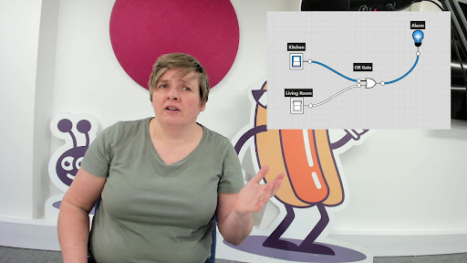
Run the cells in the section Point in time query. You can verify that you’re seeing the previous version of the table where the upsert and delete operations haven’t been applied yet.
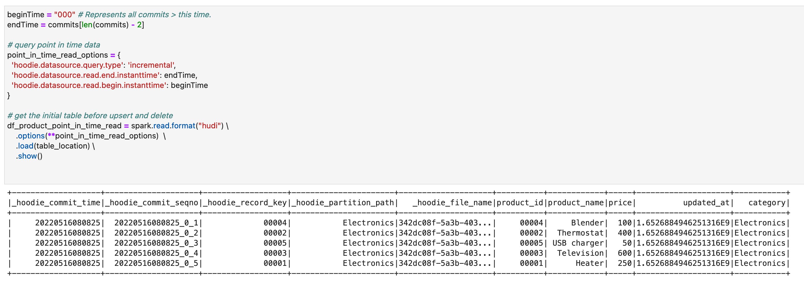
Run the cells in the section Incremental Query. You can verify that you’re seeing only the recent commit about product_id=00006.

On this notebook, you could complete the basic Spark DataFrame operations on Hudi tables.

Delta Lake

To read/write Delta Lake tables in the AWS Glue Studio notebook, complete following:

Download delta_sql.ipynb.
Open AWS Glue Studio.
Choose Jobs.
Choose Jupyter notebook, and then choose Upload and edit an existing notebook. From Choose file, select your ipynb file and choose Open, then choose Create.
On the Notebook setup page, for Job name, enter your job name.
For IAM role, select your IAM role. Choose Create job. After a short time period, the Jupyter notebook editor appears.
In the first cell, replace the placeholder with your Delta connection name, and run the cell:
%connections delta-100-byoc-connection
In the second cell, replace the S3 bucket name placeholder with your S3 bucket name, and run the cell.
Run the cells in the section Initialize SparkSession.
Run the cells in the section Clean up existing resources.
Run the cells in the section Create Delta table with sample data to create a new Delta table with sample data.
Run the cells in the section Create a Delta Lake table.
Run the cells in the section Read from Delta Lake table to verify the new Delta table. There are five records in this table.
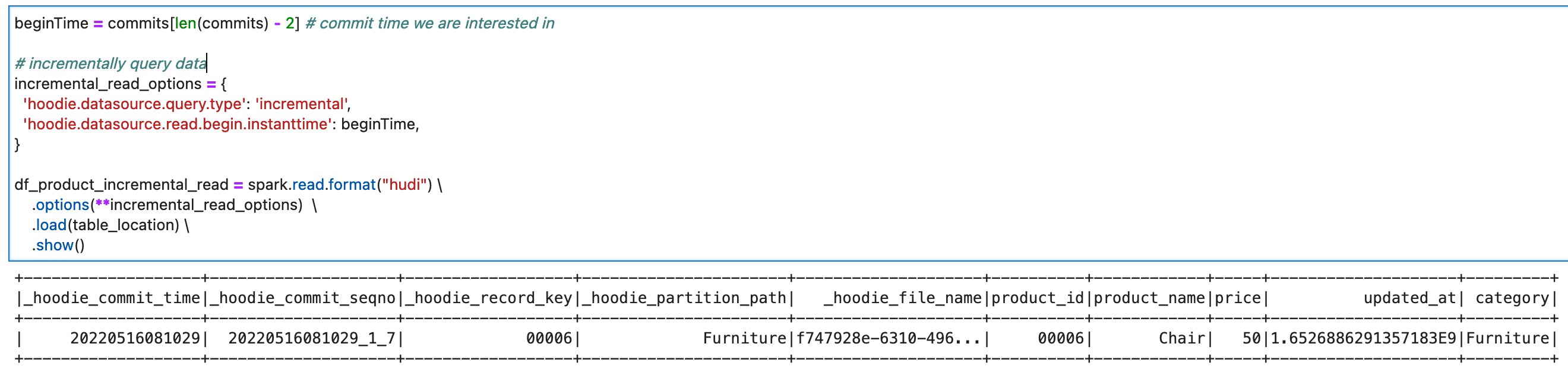
Run the cells in the section Insert records. The query inserts two new records: record_id=00006, and record_id=00007.
Run the cells in the section Update records. The query updates the price of the existing records record_id=00007, and record_id=00007 from 500 to 300.
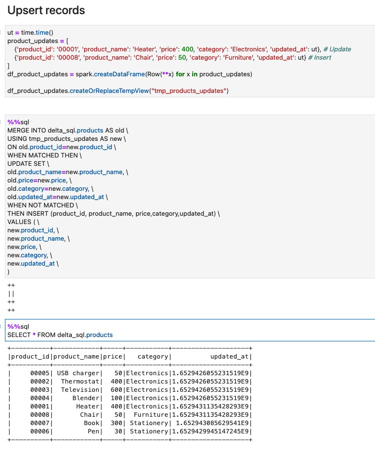
Run the cells in the section Upsert records. to see how upsert works on Delta. This code inserts one new record, and updates the one existing record. You can verify that there is a new record product_id=00008, and the existing record product_id=00001’s price has been updated from 250 to 400.
Run the cells in the section Alter DeltaLake table. The queries add one new column, and update the values in the column.
Run the cells in the section Delete records. You can verify that the record product_id=00006 because it’s product_name is Pen.
Run the cells in the section View History to describe the history of operations that was triggered against the target Delta table.

On this notebook, you could complete the basic Spark SQL operations on Delta tables.

Apache Iceberg

To read/write Apache Iceberg tables in the AWS Glue Studio notebook, complete the following:

Download iceberg_sql.ipynb.
Open AWS Glue Studio.
Choose Jobs.
Choose Jupyter notebook and then choose Upload and edit an existing notebook. From Choose file, select your ipynb file and choose Open, then choose Create.
On the Notebook setup page, for Job name, enter your job name.
For IAM role, select your IAM role. Choose Create job. After a short time period, the Jupyter notebook editor appears.
In the first cell, replace the placeholder with your Delta connection name, and run the cell:
%connections iceberg-0131-byoc-connection (Alternatively you can use your connection name created from the marketplace connector).
In the second cell, replace the S3 bucket name placeholder with your S3 bucket name, and run the cell.
Run the cells in the section Initialize SparkSession.
Run the cells in the section Clean up existing resources.
Run the cells in the section Create Iceberg table with sample data to create a new Iceberg table with sample data.
Run the cells in the section Read from Iceberg table.
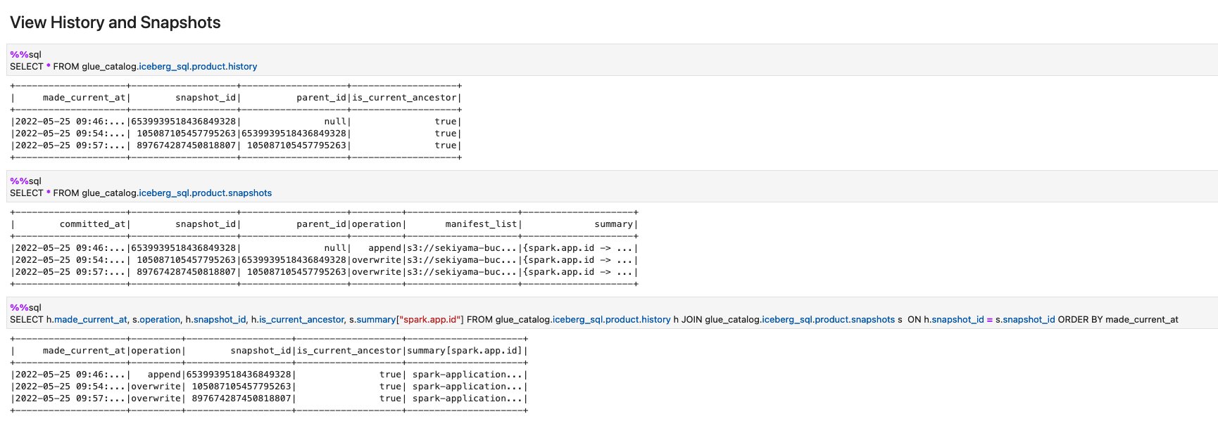
Run the cells in the section Upsert records into Iceberg table.
Run the cells in the section Delete records.
Run the cells in the section View History and Snapshots.

On this notebook, you could complete the basic Spark SQL operations on Iceberg tables.

Conclusion

This post summarized how to utilize Apache Hudi, Delta Lake, and Apache Iceberg on AWS Glue platform, as well as demonstrate how each format works with a Glue Studio notebook. You can start using those data lake formats easily in Spark DataFrames and Spark SQL on the Glue jobs or the Glue Studio notebooks.

This post focused on interactive coding and querying on notebooks. The upcoming part 2 will focus on the experience using AWS Glue Studio Visual Editor and Glue DynamicFrames for customers who prefer visual authoring without the need to write code.

About the Authors

Noritaka Sekiyama is a Principal Big Data Architect on the AWS Glue team. He enjoys learning different use cases from customers and sharing knowledge about big data technologies with the wider community.

Dylan Qu is a Specialist Solutions Architect focused on Big Data & Analytics with AWS. He helps customers architect and build highly scalable, performant, and secure cloud-based solutions on AWS.

Monjumi Sarma is a Data Lab Solutions Architect at AWS. She helps customers architect data analytics solutions, which gives them an accelerated path towards modernization initiatives.

How Plugsurfing doubled performance and reduced cost by 70% with purpose-built databases and AWS Graviton

2022-07-18 Anand Shah

Post Syndicated from Anand Shah original https://aws.amazon.com/blogs/big-data/how-plugsurfing-doubled-performance-and-reduced-cost-by-70-with-purpose-built-databases-and-aws-graviton/

Plugsurfing aligns the entire car charging ecosystem—drivers, charging point operators, and carmakers—within a single platform. The over 1 million drivers connected to the Plugsurfing Power Platform benefit from a network of over 300,000 charging points across Europe. Plugsurfing serves charging point operators with a backend cloud software for managing everything from country-specific regulations to providing diverse payment options for customers. Carmakers benefit from white label solutions as well as deeper integrations with their in-house technology. The platform-based ecosystem has already processed more than 18 million charging sessions. Plugsurfing was acquired fully by Fortum Oyj in 2018.

Plugsurfing uses Amazon OpenSearch Service as a central data store to store 300,000 charging stations’ information and to power search and filter requests coming from mobile, web, and connected car dashboard clients. With the increasing usage, Plugsurfing created multiple read replicas of an OpenSearch Service cluster to meet demand and scale. Over time and with the increase in demand, this solution started to become cost exhaustive and limited in terms of cost performance benefit.

AWS EMEA Prototyping Labs collaborated with the Plugsurfing team for 4 weeks on a hands-on prototyping engagement to solve this problem, which resulted in 70% cost savings and doubled the performance benefit over the current solution. This post shows the overall approach and ideas we tested with Plugsurfing to achieve the results.

The challenge: Scaling higher transactions per second while keeping costs under control

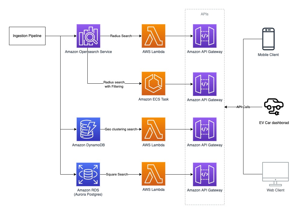
One of the key issues of the legacy solution was keeping up with higher transactions per second (TPS) from APIs while keeping costs low. The majority of the cost was coming from the OpenSearch Service cluster, because the mobile, web, and EV car dashboards use different APIs for different use cases, but all query the same cluster. The solution to achieve higher TPS with the legacy solution was to scale the OpenSearch Service cluster.

The following figure illustrates the legacy architecture.

Legacy Architecture

Plugsurfing APIs are responsible for serving data for four different use cases:

Radius search – Find all the EV charging stations (latitude/longitude) with in x km radius from the point of interest (or current location on GPS).
Square search – Find all the EV charging stations within a box of length x width, where the point of interest (or current location on GPS) is at the center.
Geo clustering search – Find all the EV charging stations clustered (grouped) by their concentration within a given area. For example, searching all EV chargers in all of Germany results in something like 50 in Munich and 100 in Berlin.
Radius search with filtering – Filter the results by EV charger that are available or in use by plug type, power rating, or other filters.

The OpenSearch Service domain configuration was as follows:

m4.10xlarge.search x 4 nodes
Elasticsearch 7.10 version
A single index to store 300,000 EV charger locations with five shards and one replica
A nested document structure

The following code shows the example document

{
   "locationId":"location:1",
   "location":{
      "latitude":32.1123,
      "longitude":-9.2523
   },
   "adress":"parking lot 1",
   "chargers":[
      {
         "chargerId":"location:1:charger:1",
         "connectors":[
            {
               "connectorId":"location:1:charger:1:connector:1",
               "status":"AVAILABLE",
               "plug_type":"Type A"
            }
         ]
      }
   ]
}

Solution overview

AWS EMEA Prototyping Labs proposed an experimentation approach to try three high-level ideas for performance optimization and to lower overall solution costs.

We launched an Amazon Elastic Compute Cloud (EC2) instance in a prototyping AWS account to host a benchmarking tool based on k6 (an open-source tool that makes load testing simple for developers and QA engineers) Later, we used scripts to dump and restore production data to various databases, transforming it to fit with different data models. Then we ran k6 scripts to run and record performance metrics for each use case, database, and data model combination. We also used the AWS Pricing Calculator to estimate the cost of each experiment.

Experiment 1: Use AWS Graviton and optimize OpenSearch Service domain configuration

We benchmarked a replica of the legacy OpenSearch Service domain setup in a prototyping environment to baseline performance and costs. Next, we analyzed the current cluster setup and recommended testing the following changes:

Use AWS Graviton based memory optimized EC2 instances (r6g) x 2 nodes in the cluster
Reduce the number of shards from five to one, given the volume of data (all documents) is less than 1 GB
Increase the refresh interval configuration from the default 1 second to 5 seconds
Denormalize the full document; if not possible, then denormalize all the fields that are part of the search query
Upgrade to Amazon OpenSearch Service 1.0 from Elasticsearch 7.10

Plugsurfing created multiple new OpenSearch Service domains with the same data and benchmarked them against the legacy baseline to obtain the following results. The row in yellow represents the baseline from the legacy setup; the rows with green represent the best outcome out of all experiments performed for the given use cases.

DB Engine	Version	Node Type	Nodes in Cluster	Configurations	Data Modeling	Radius req/sec	Filtering req/sec	Performance Gain %
Elasticsearch	7.1	m4.10xlarge	4	5 shards, 1 replica	Nested	2841	580	0
Amazon OpenSearch Service	1.0	r6g.xlarge	2	1 shards, 1 replica	Nested	850	271	32.77
Amazon OpenSearch Service	1.0	r6g.xlarge	2	1 shards, 1 replica	Denormalized	872	670	45.07
Amazon OpenSearch Service	1.0	r6g.2xlarge	2	1 shards, 1 replica	Nested	1667	474	62.58
Amazon OpenSearch Service	1.0	r6g.2xlarge	2	1 shards, 1 replica	Denormalized	1993	1268	95.32

Plugsurfing was able to gain 95% (doubled) better performance across the radius and filtering use cases with this experiment.

Experiment 2: Use purpose-built databases on AWS for different use cases

We tested Amazon OpenSearch Service, Amazon Aurora PostgreSQL-Compatible Edition, and Amazon DynamoDB extensively with many data models for different use cases.

We tested the square search use case with an Aurora PostgreSQL cluster with a db.r6g.2xlarge single node as the reader and a db.r6g.large single node as the writer. The square search used a single PostgreSQL table configured via the following steps:

Create the geo search table with geography as the data type to store latitude/longitude:

CREATE TYPE status AS ENUM ('available', 'inuse', 'out-of-order');

CREATE TABLE IF NOT EXISTS square_search
(
id     serial PRIMARY KEY,
geog   geography(POINT),
status status,
data   text -- Can be used as json data type, or add extra fields as flat json
);

Create an index on the geog field:

CREATE INDEX global_points_gix ON square_search USING GIST (geog);

Query the data for the square search use case:

SELECT id, ST_AsText(geog), status, datafrom square_search
where geog && ST_MakeEnvelope(32.5,9,32.8,11,4326) limit 100;

We achieved an eight-times greater improvement in TPS for the square search use case, as shown in the following table.

DB Engine	Version	Node Type	Nodes in Cluster	Configurations	Data modeling	Square req/sec	Performance Gain %
Elasticsearch	7.1	m4.10xlarge	4	5 shards, 1 replica	Nested	412	0
Aurora PostgreSQL	13.4	r6g.large	2	PostGIS, Denormalized	Single table	881	213.83
Aurora PostgreSQL	13.4	r6g.xlarge	2	PostGIS, Denormalized	Single table	1770	429.61
Aurora PostgreSQL	13.4	r6g.2xlarge	2	PostGIS, Denormalized	Single table	3553	862.38

We tested the geo clustering search use case with a DynamoDB model. The partition key (PK) is made up of three components: <zoom-level>:<geo-hash>:<api-key>, and the sort key is the EV charger current status. We examined the following:

The zoom level of the map set by the user
The geo hash computed based on the map tile in the user’s view port area (at every zoom level, the map of Earth is divided into multiple tiles, where each tile can be represented as a geohash)
The API key to identify the API user

Partition Key: String	Sort Key: String	total_pins: Number	filter1_pins: Number	filter2_pins: Number	filter3_pins: Number
5:gbsuv:api_user_1	Available	100	50	67	12
5:gbsuv:api_user_1	in-use	25	12	6	1
6:gbsuvt:api_user_1	Available	35	22	8	0
6:gbsuvt:api_user_1	in-use	88	4	0	35

The writer updates the counters (increment or decrement) against each filter condition and charger status whenever the EV charger status is updated at all zoom levels. With this model, the reader can query pre-clustered data with a single direct partition hit for all the map tiles viewable by the user at the given zoom level.

The DynamoDB model helped us gain a 45-times greater read performance for our geo clustering use case. However, it also added extra work on the writer side to pre-compute numbers and update multiple rows when the status of a single EV charger is updated. The following table summarizes our results.

DB Engine	Version	Node Type	Nodes in Cluster	Configurations	Data modeling	Clustering req/sec	Performance Gain %
Elasticsearch	7.1	m4.10xlarge	4	5 shards, 1 replica	Nested	22	0
DynamoDB	NA	Serverless	0	100 WCU, 500 RCU	Single table	1000	4545.45

Experiment 3: Use AWS Lambda@Edge and AWS Wavelength for better network performance

We recommended that Plugsurfing use Lambda@Edge and AWS Wavelength to optimize network performance by shifting some of the APIs at the edge to closer to the user. The EV car dashboard can use the same 5G network connectivity to invoke Plugsurfing APIs with AWS Wavelength.

Post-prototype architecture

The post-prototype architecture used purpose-built databases on AWS to achieve better performance across all four use cases. We looked at the results and split the workload based on which database performs best for each use case. This approach optimized performance and cost, but added complexity on readers and writers. The final experiment summary represents the database fits for the given use cases that provide the best performance (highlighted in orange).

Plugsurfing has already implemented a short-term plan (light green) as an immediate action post-prototype and plans to implement mid-term and long-term actions (dark green) in the future.

DB Engine	Node Type	Configurations	Radius req/sec	Radius Filtering req/sec	Clustering req/sec	Square req/sec	Monthly Costs $	Cost Benefit %	Performance Gain %
Elasticsearch 7.1	m4.10xlarge x4	5 shards	2841	580	22	412	9584,64	0	0
Amazon OpenSearch Service 1.0	r6g.2xlarge x2	1 shard Nested	1667	474	34	142	1078,56	88,75	-39,9
Amazon OpenSearch Service 1.0	r6g.2xlarge x2	1 shard	1993	1268	125	685	1078,56	88,75	5,6
Aurora PostgreSQL 13.4	r6g.2xlarge x2	PostGIS	0	0	275	3553	1031,04	89,24	782,03
DynamoDB	Serverless	100 WCU 500 RCU	0	0	1000	0	106,06	98,89	4445,45
Summary	.	.	2052	1268	1000	3553	2215,66	76,88	104,23

The following diagram illustrates the updated architecture.

Post Prototype Architecture

Conclusion

Plugsurfing was able to achieve a 70% cost reduction over their legacy setup with two-times better performance by using purpose-built databases like DynamoDB, Aurora PostgreSQL, and AWS Graviton based instances for Amazon OpenSearch Service. They achieved the following results:

The radius search and radius search with filtering use cases achieved better performance using Amazon OpenSearch Service on AWS Graviton with a denormalized document structure
The square search use case performed better using Aurora PostgreSQL, where we used the PostGIS extension for geo square queries
The geo clustering search use case performed better using DynamoDB

Learn more about AWS Graviton instances and purpose-built databases on AWS, and let us know how we can help optimize your workload on AWS.

About the Author

Anand Shah is a Big Data Prototyping Solution Architect at AWS. He works with AWS customers and their engineering teams to build prototypes using AWS Analytics services and purpose-built databases. Anand helps customers solve the most challenging problems using art-of-the-possible technology. He enjoys beaches in his leisure time.

Implementing the AWS Well-Architected Custom Lens lifecycle in your organization

2022-07-18 Robert Hoffman

Post Syndicated from Robert Hoffman original https://aws.amazon.com/blogs/architecture/implementing-the-aws-well-architected-custom-lens-lifecycle-in-your-organization/

In this blog post, we present a lifecycle that helps you build, validate, and improve your own AWS Well-Architected Custom Lens, in order to roll it out across your whole organization. The AWS Well-Architected Custom Lens is a new feature of the AWS Well-Architected Tool that lets you bring your own best practices to complement the existing Well-Architected Framework.

The Custom Lens lifecycle: how a Custom Lens can benefit your organization

Figure 1. The AWS Well-Architected Custom Lens lifecycle

Each organization has its own requirements, processes, best practices, and tools, but the information can be spread over many systems and knowledge bases. A Custom Lens can capture the specifics of a working environment and let coworkers access this information in a single place—from the AWS console—without the need to go to a separate tool. A Custom Lens can be created in a central management account and securely shared with other accounts.

A Custom Lens can be updated periodically as either a major or minor version. If it is a minor version, the change is automatically applied to all accounts that the lens has been shared with. If it is a major version, the user has to accept the updated Custom Lens and a summary of the changes is displayed to the user. Accepting the changes then applies the update for existing workload reviews, and prompts the user to review the workload. Thus, updating a Custom Lens is an effective mechanism to continuously inform teams about new best practices.

In addition, maintaining and improving a Custom Lens continuously helps to identify gaps in organization-wide tooling, guidance, or documentation. You can aggregate feedback and metrics from reviews that have been performed and use it to drive the improvement process of the content. More importantly, the gathered metrics help measure the overall adherence to best practices and requirements in your organization. If you focus on creating clear, concise, and actionable content for your Custom Lens, the time needed to identify and implement improvements is reduced. As teams realize the value of the Custom Lens, more reviews will be performed, and you will receive more data to construct a comprehensive view.

1. Plan

The Plan phase identifies the benefits that a Custom Lens can provide your organization by identifying current gaps. You also define the scope of your Custom Lens, which is the type of content that supports your desired business outcomes. Depending on the scope, you need to identify the appropriate stakeholders and gain support for the initiative.

2. Implement

In the Implement phase, content is created for the Custom Lens with a working group. While doing this, you can identify missing supplementary artefacts, like documentation or tooling. If that is the case, you can create these artefacts and link to them from the Custom Lens Improvement Plan.

As part of the implementation, the Custom Lens is created by uploading a JSON file in the appropriate format to a central management account, then, sharing the lens with the organization’s AWS accounts. You can share the Custom Lens with IAM Principals, such as users, roles, and AWS accounts. For broader and more efficient sharing, you now have the ability to scale by sharing your Custom Lens with individual organizational units or the entire AWS Organizations. This feature reduces management overhead and removes the need for a custom automation.

3. Measure

The Measure phase aggregates feedback and metrics from reviews that have been performed with your Custom Lens; this information is used to drive the improvement process.

The Well-Architected Tool offers a way to share workload reviews, and you can use this to share all reviews with a central AWS account. You can then analyze the reviews in the central account by extracting the data and analyzing it, for example, by building a dashboard. The Well-Architected Lab for building custom reports provides a solution that can be implemented.

4. Improve

In the Improve phase, the gathered metrics and feedback are used to identify areas for future improvement. For example, you might find common gaps among the performed workload reviews, where the same best practices are not fulfilled. When you investigate the root cause, you can learn that the existing content lacks clarity or that the suggested tools are difficult to use.

In addition, improvements, such as content gaps that were not addressed during the first iteration of the Custom Lens, can be added to the backlog before you repeat the cycle.

To roll out changes of your Custom Lens in an automated and repeatable fashion, you can implement the architecture depicted in Figure 2.

Figure 2. Combining AWS CodeCommit with AWS Lambda to update your Custom Lens whenever a file change is pushed to the code repository

This architecture enables automated releases of new versions of your Custom Lens whenever you commit an updated JSON file to the code repository. In detail, the steps are:

The JSON file of your Custom Lens is stored in an AWS CodeCommit repository. An author pushes an updated version of the file to the repository.
The CodeCommit repository is configured with a trigger action that invokes an AWS Lambda function on each commit.
The Lambda function downloads the updated file by using the GetFile API of CodeCommit. Then, the Lambda function imports the updated Custom Lens and publishes it as a new version by using ImportLens and CreateLensVersion APIs of the AWS Well-Architected Tool, then shares the Custom Lens using CreateLensShare.
The updated Custom Lens is available in all accounts that the lens has been shared with.
Reviewers can create new workload reviews with the Custom Lens or upgrade to the newest version for existing workload reviews.

Conclusion

In this blog post, we walked you through the Custom Lens lifecycle, a process to create and continuously improve a Custom Lens for your organization. If you have a special software development lifecycle, a customized security and compliance framework, or other highly specific requirements or best practices that you want disseminated and measurable, learn more about how to create a Custom Lens in the Well-Architected Tool.

AWS Well-Architected is a set of guiding design principles developed by AWS to help organizations build secure, high-performing, resilient, and efficient infrastructure for a variety of applications and workloads. Use the AWS Well-Architected Tool to review your workloads periodically to address important design considerations and ensure that they follow the best practices and guidance of the AWS Well-Architected Framework. For follow up questions or comments, join our growing community on AWS re:Post.

Use Security Hub custom actions to remediate S3 resources based on Macie discovery results

2022-07-18 Jonathan Nguyen

Post Syndicated from Jonathan Nguyen original https://aws.amazon.com/blogs/security/use-security-hub-custom-actions-to-remediate-s3-resources-based-on-macie-discovery-results/

The amount of data available to be collected, stored and processed within an organization’s AWS environment can grow rapidly and exponentially. This increases the operational complexity and the need to identify and protect sensitive data. If your security teams need to review and remediate security risks manually, it would either take a large team or the actions might not be timely. There is also a chance that with manual operation, a step could be missed or the incorrect action could be taken. As a result, your security teams will need an automated and scalable way to support these operations efficiently.

Amazon Macie is a fully managed data security and data privacy service that uses machine learning and pattern matching to discover and protect your sensitive data in AWS. Macie generates findings for sensitive data in an S3 object or a potential issue with the security or privacy of an S3 bucket. AWS Security Hub allows you to gain a centralized view into the security posture across your AWS environment by aggregating security findings from various AWS services and partner products, including Amazon Macie. Security Hub also includes the custom actions feature, which you can use to create actions for response and remediation to selected findings within the Security Hub console in an efficient and consistent manner.

It is important for your security teams to create effective and standardized mechanisms for taking action against Macie findings to ensure that data remains secure. By using Security Hub custom actions, you can have predefined actions for the security team to take against Macie findings without having to manually find and remediate the resources.

This blog post provides you with an example solution for responding to Macie sensitive data findings and policy findings in Security Hub by using custom actions. I will walk through the components of the solution, as well as opportunities where resources can be customized for your specific use case.

Prerequisites

You must have AWS Security Hub and Amazon Macie enabled in the AWS account where you are deploying this solution.

Solution overview

In this solution, you’ll use a combination of Security Hub custom actions, Amazon EventBridge, and AWS Lambda to take action on Macie findings in Security Hub. You will be working with the findings within the same AWS account where you deployed the solution.

Macie generates two categories of findings relating to different resources, which will require different remediation actions.

Policy finding is a detailed report of a potential policy violation or issue with the security or privacy of an Amazon Simple Storage Service (Amazon S3) bucket.
Sensitive data finding is a detailed report of sensitive data in an S3 object.

A full list of Macie finding types can be found in the Macie User guide.

For the two Macie finding categories, there is an associated Security Hub custom action:

Custom action for sensitive data finding (S3 object) – When the security team selects this custom action, the action invokes a Lambda function that will take the following steps on the S3 object in the Macie finding:
1. Tag the object with the Security Hub finding ID
2. Encrypt the S3 object with a different customer-managed KMS key
3. Update the Security Hub finding workflow status to RESOLVED
Custom action for policy finding (S3 bucket). When you select this this custom action, it invokes a Lambda function that will take the following steps on the S3 bucket in the Macie finding:
1. Tag the object with the Security Hub finding ID
2. Update the S3 bucket configuration to:
  - Enable default encryption
  - Enable public access block
3. Update the Security Hub finding workflow status to RESOLVED

The solution is configured to take action within the AWS account where the finding and corresponding resource is generated. In order to enable cross-account remediation, you will need to deploy an additional IAM role for the automation to assume and provision a KMS key to use for encryption.

Note: The custom actions in this solution are meant to be examples of actions to take against Macie policy and sensitive data findings. These actions will be different depending on your use-case and environment. You will also need to review and update the associated Lambda function execution role IAM policies accordingly.

Solution architecture

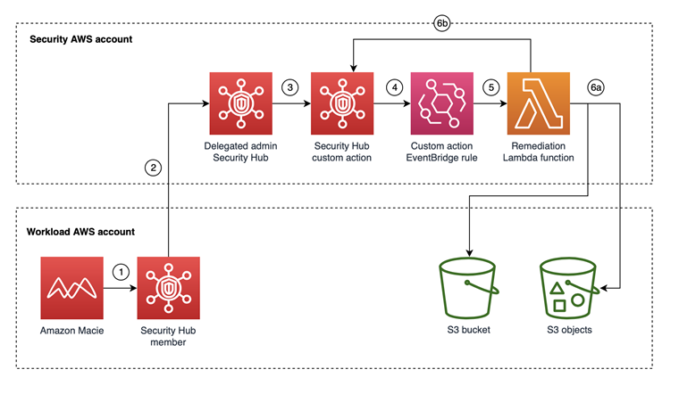
Figure 1: Resources deployed in the Security AWS account taking action on resources identified in the Workload AWS account

Figure 1 shows the architecture for the solution. The workflow is as follows:

A Macie job runs and creates findings, which are sent to Security Hub in the same AWS account as the Macie finding.
The delegated administrator Security Hub account combines findings across all member Security Hub accounts, including Macie findings.
The security team reviews the Macie findings in the Security Hub delegated administrator account and determines to take remediation actions for a finding by selecting the finding and then selecting the appropriate Security Hub custom action.
The Security Hub custom action sends the finding to the EventBridge rule, which is linked to the Lambda function.
The EventBridge rule invokes the Lambda function to take action against the resources from the Macie finding.
The Lambda function will:
1. Take action for the S3 resource
2. Mark the Macie finding as resolved in the delegated administrator Security Hub account

The solution is currently intended to work in a single Region. In order to enable this solution across Regions, you will need to change the Remediation Lambda function code for any regional resources used for remediation actions (i.e. AWS Key Management Service).

Deploy the solution

You can deploy the solution through either the AWS Management Console or the AWS Cloud Development Kit (AWS CDK).

To deploy the solution by using the AWS Management Console

In your security tooling account, launch the AWS CloudFormation template by choosing the following Launch Stack button. It will take approximately 10 minutes for the CloudFormation stack to complete.

Note: The stack will launch in the N. Virginia (us-east-1) Region. To deploy this solution into other AWS Regions, download the solution’s CloudFormation template, modify it, and deploy it to the selected Region.
(OPTIONAL) If you want to enable cross-account remediation, launch the following AWS CloudFormation template in the AWS account where you want to be able to take remediation actions. You can also use AWS CloudFormation StackSets if deploying to multiple AWS accounts.

To deploy the solution by using AWS CDK

You can find the latest code in our GitHub repository, where you can also contribute to the sample code. The following commands show how to deploy the solution by using the AWS CDK. First, the CDK initializes your environment and uploads the AWS Lambda assets to Amazon S3. Then, you can deploy the solution to your account. Make sure to replace <AWS_ACCOUNT> with the account number, and replace <REGION> with the AWS Region that you want the solution deployed to.

Run the following commands in your terminal while authenticated in the security tooling AWS account:
cdk bootstrap aws://<Security_Tooling_AWS_ACCOUNT>/<REGION>

cdk deploy MacieRemediationStack
(OPTIONAL) If you want to enable cross-account remediation, Run the following commands in your terminal while authenticated to member AWS account:
cdk bootstrap aws://<Member_AWS_ACCOUNT>/<REGION>

cdk deploy MacieRemediationIAMStack –parameters solutionaccount=<Security_Tooling_AWS_ACCOUNT>

Solution walkthrough and validation

Now that you’ve successfully deployed the solution, you can see things in action. You have two options for testing the workflow on your own:

Use a sample event, generated by a Macie finding in Security Hub, and invoke the Lambda function that is tied to the Security Hub custom action.

Note: If using sample events, you can replace the values for the resources with real resources. Otherwise, you will not be able to see the Lambda function successfully take action because the resource in your sample event may not exist.
Generate demo Macie findings in Security Hub by using this sample data for Amazon Macie.

I have existing findings for Macie generated in my AWS account, and in the procedures in this section, I’ll walk through taking action against these.

Note: If you set up Macie and Security Hub in a delegated administrator and member model that ingests findings from other AWS accounts, the IAM remediation roles for the S3 bucket and S3 objects must be deployed in the member accounts.

Review deployed resources in the AWS console

Before taking action on your sample findings, review the deployed resources that you’ll use.

To review deployed resources

In the AWS account console where the automation was deployed, go to Security Hub, choose Settings, and then choose Custom actions. You should see two custom actions:
- Macie Policy Finding
  - arn:aws:securityhub:<region>:<account-id>:action/custom/MacieS3BucketPolicy
- Macie Data Finding
  - arn:aws:securityhub:<region>:<account-id>:action/custom/MacieSensitiveData
    
    Figure 2: Custom actions in Security Hub
Navigate to the EventBridge console and then choose Rules. You should see four rules:
- Disabled – These are disabled by default during deployment
  - Autoremediate_Macie_Policy_Finding
  - Autoremediate_Macie_Sensitive_Data_Finding
    
    Figure 3: Disabled EventBridge rules for autoremediation of Macie findings in Security Hub
- Enabled – These are enabled by default during deployment:
  - Custom_Action_Macie_Policy_Finding
  - Custom_Action_Macie_Sensitive_Data_Finding
    
    Figure 4: Enabled EventBridge rules tied to the Security Hub custom actions
In the enabled EventBridge rules, you should see the corresponding Security Hub custom action Amazon Resource Names (ARNs) in the rule event pattern.

Figure 5: Enabled EventBridge rule event pattern for the Security Hub custom action

Take action on an Amazon Macie object or policy finding

Each Security Hub custom action invokes a corresponding Lambda function that is configured as a target in the EventBridge rule. The Lambda function parses the information in the Macie finding from Security Hub to take action.

Each Security Hub custom action is specific to either an S3 object or an S3 bucket. If you attempt a custom action meant for an S3 object against a Macie policy finding, this will successfully initiate the custom action, but the Lambda function that is invoked will be unsuccessful.

If the Macie finding is specific to an S3 object, the title will display “The S3 object …,” whereas if the Macie finding is for a policy finding, the title will display information for an S3 bucket.

To take action on findings

In the AWS account console where the automation was deployed, navigate to AWS Security Hub, and then choose Findings.
Filter the findings by setting Product Name to Macie.

Figure 6: Filter for Macie findings in Security Hub
Select the checkbox for either a Macie policy finding or a sensitive data finding; this will select a custom action. After you select the action, there is no confirmation step, and the action will invoke the Lambda function.

Figure 7: Validate Custom Action has sent the finding to Amazon CloudWatch Events (EventBridge rule)

Review and validate the Security Hub custom action on target resources

In order to validate or troubleshoot the solution, you need to review whether the Lambda function was able to take action against the resources in the Security Hub finding for Macie.

To validate or troubleshoot the custom action

For validation of sensitive data finding remediation, review S3 object configuration:
1. Navigate to the Amazon S3 console.
2. Choose the S3 object in the Macie finding.
3. Choose the Properties tab and review the following fields:
  - Tags should be set to SH_Finding_ID.
  - AWS KMS key ARN should be set to the KMS key with the alias `macie_key`
    1. Click on the KMS key ARN and validate the key’s alias is the key deployed in the solution
For validation of policy finding remediation, review the S3 bucket configuration:
1. Navigate to the Amazon S3 console.
2. Choose the S3 bucket in the Macie finding.
3. Choose the Properties tab and review the following fields:
  - Tags should be set to SH_Finding_ID.
  - Default Encryption should be set to Enabled.
4. Choose the Permissions tab and review the following fields:
  - Block public access should be set to On.
For troubleshooting, you can review the CloudWatch logs for the Lambda function:
1. Navigate to the CloudWatch console.
2. Choose /aws/lambda/Remediate_Macie_S3_Bucket.
3. Choose the most recent log stream and review the logs to see what actions were taken on the resources.

Next steps and customization

The solution in this post has a custom action for an S3 object and an S3 bucket, and is meant to serve as a template. You could modify the Lambda functions associated with the custom actions to take different or additional actions that are specific to your environment and data classification.

Additionally, I walked through specific Security Hub custom actions for Macie policy (bucket) or sensitive data (objects) findings. If you have defined actions to take for both, you could consolidate the custom actions and invoke a Lambda function that parses information from the Security Hub Macie finding to determine if it is a policy or sensitive data finding.

The two disabled EventBridge rules deployed as part of the solution are examples that can be leveraged for auto-remediation. After you use Security Hub’s custom actions to remediate findings, your security team could start to see a trend where you always want to take specific actions and enable the EventBridge rules to take action without requiring your security team to select a custom action in Security Hub in the AWS console.

Autoremediate_Macie_Policy_Finding
Autoremediate_Macie_Sensitive_Data_Finding

Conclusion

In this post, you deployed a solution to allow your security team to take automated actions against a Macie sensitive data and policy finding from Security Hub by using custom actions in the AWS console. We walked through what the solution does and how the solution can be customized to your use case.

If you have feedback about this post, submit comments in the Comments section below. If you have any questions about this post, start a thread on the AWS Security Hub forum or Amazon Macie forum.

Want more AWS Security news? Follow us on Twitter.

AWS Week In Review – July 18, 2022

2022-07-18 Channy Yun

Post Syndicated from Channy Yun original https://aws.amazon.com/blogs/aws/aws-week-in-review-july-18-2022/

Last week, AWS Summit New York was held in person at the Javits Center with thousands of attendees and over 100 sponsors and partners. During the keynote, Martin Beeby, AWS Principal Developer Advocate, talked about how innovations in cloud infrastructure enable customers to adapt to challenges and seize new opportunities. It included Liz Fong-Jones‘s great migration story of AWS Graviton in Honeycomb and Elliott Cordo‘s story of improving pharmacy experiences using AWS analytics and machine learning services in Capsule.

Watch the full keynote video!

A Recap of AWS Summit NY Announcements
During the keynote, we announced the general availability of some new services:

Amazon Redshift Serverless – This serverless option lets you analyze data at any scale without having to manage data warehouse infrastructure. You can now create multiple serverless endpoints per AWS account and Region using namespaces and workgroups and enjoy reducing serverless compute costs compared to the preview. To learn more, check out Danilio’s blog post, this demo video, and the latest episode of The Official AWS Podcast. We also introduced new features of row-level security (RLS), which implement fine-grained access to the rows in tables, and automated materialized view to lower query latency for repeatable workloads.

AWS Cloud WAN – This new network service makes it easy to build and operate wide area networks (WAN) that connect your data centers and branch offices, as well as multiple VPCs in multiple AWS Regions. To learn more, read Seb’s blog post.

Amazon DevOps Guru’s Log Anomaly Detection and Recommendations – This new feature identifies anomalies such as increased latency, error rates, and resource constraints within your app and then sends alerts with a description and actionable recommendations for remediation. To learn more, see Donnie’s blog post as a new News Blog writer.

Last Week’s Launches
Here are some other launches that caught my attention last week:

AWS AppConfig, a feature of AWS Systems Manager, makes it easy for customers to quickly and safely configure, validate, and deploy feature flags and application configuration. Now, we have announced AWS AppConfig Extensions, a new capability that allows customers to enhance and extend the capabilities of feature flags and dynamic runtime configuration data.

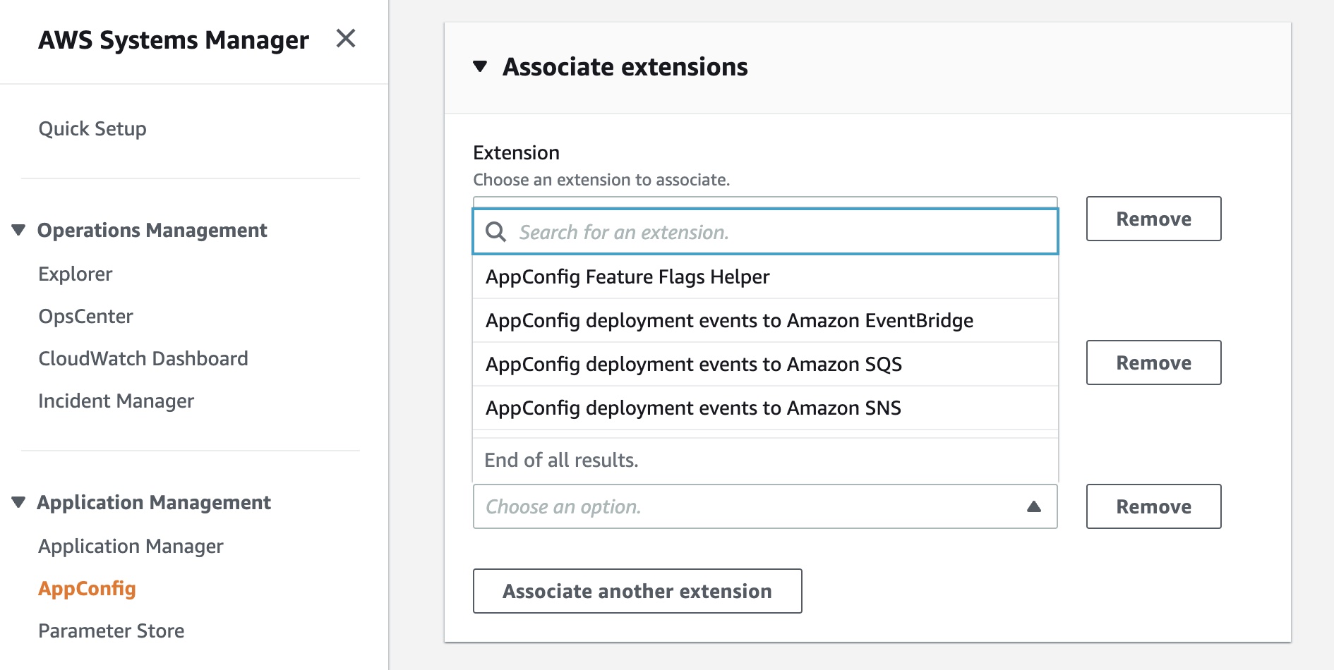
Available extensions at launch include AppConfig Notification extensions that push messages about configuration updates to Amazon EventBridge, Amazon SNS, Amazon SQS, or a Jira extension to track Feature Flag changes in AppConfig as Atlassian’s Jira issues. To get started, read Announcing AWS AppConfig Extensions and AppConfig Extensions.

Amazon VPC Flow Logs for Transit Gateway is a new capability that allows customers to gain deeper visibility and insights into network traffic on AWS Transit Gateway. With this feature, Transit Gateway can export detailed information, such as source/destination IPs, ports, protocols, traffic counters, timestamps, and various metadata for all of the network flow traversing through the Transit Gateway. To learn more, read Introducing VPC Flow Logs for AWS Transit Gateway and Logging network traffic using Transit Gateway Flow Logs.

AWS Lambda Powertools for TypeScript is an open-source developer library that can help you incorporate Well-Architected Serverless best practices focusing on three observability features: distributed tracing (Tracer), structured logging (Logger), and asynchronous business and application metrics (Metrics). Powertools is also available in the Python and Java programming languages. To learn more, see the blog post Simplifying serverless best practices with AWS Lambda Powertools for TypeScript. You can submit feedback, ideas, and issues directly on our GitHub project.

AWS re:Post is a vibrant Q&A community that helps you become even more successful on AWS. You can now add a profile picture or avatar to your account and add inline images such as diagrams or screenshots to support your questions or answers. Add your profile picture and start using inline images today!

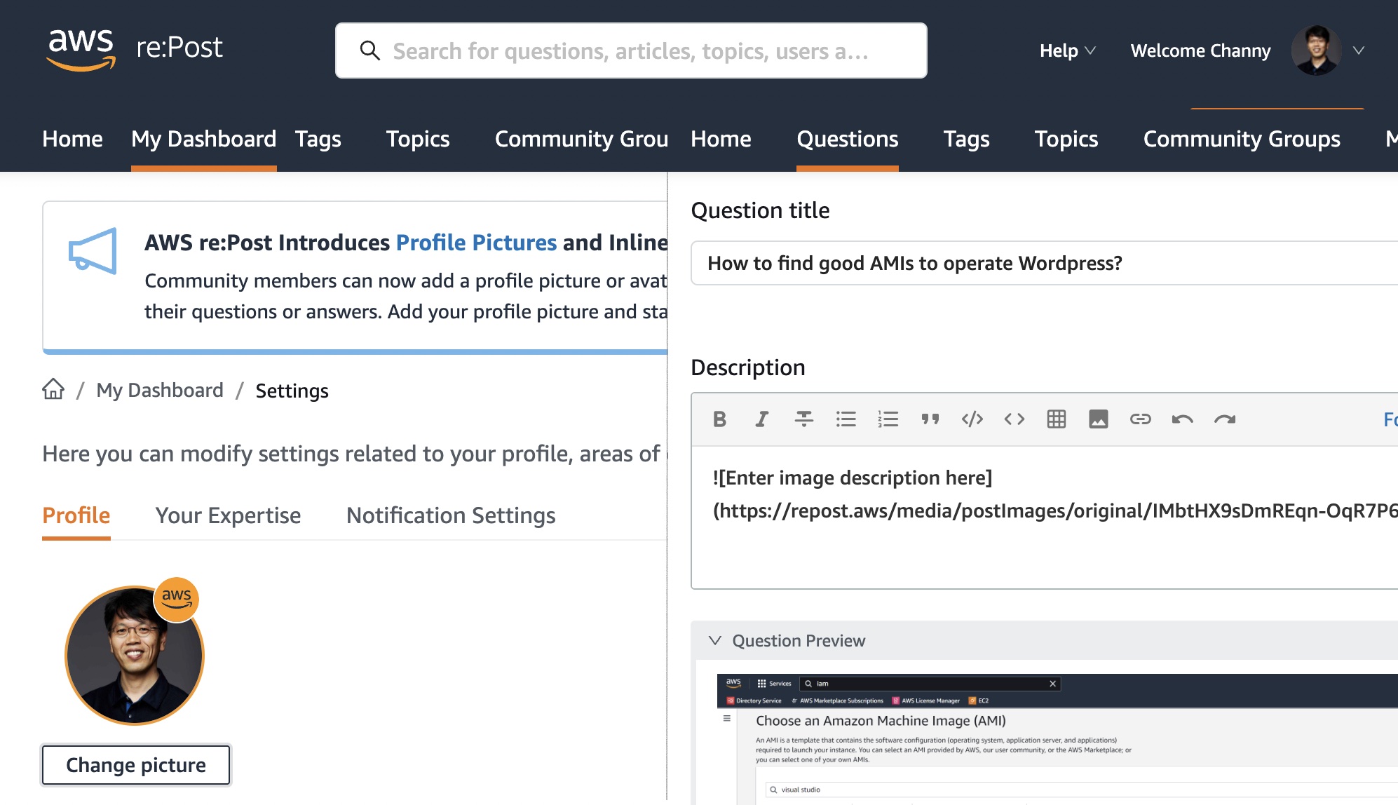
For a full list of AWS announcements, be sure to keep an eye on the What’s New at AWS page.

Other AWS News
Here are some news, blog posts, and video series for you to know:

In July 2021, we notified users about the end of support for Internet Explorer 11, which is now approaching on July 31, 2022. The browser will no longer be supported in the AWS Management Console, web-based services such as Amazon QuickSight, Amazon Chime, Amazon Honeycode, and some other AWS websites. After that date, we can no longer guarantee that the features and webpages will function properly on IE 11. For more information, please visit AWS Supported Browsers.

In fall 2021, we began offering a free multi-factor authentication (MFA) security key to AWS account owners in the United States. Now eligible customers can order the free MFA security key through the ordering portal in the AWS Management Console. At this time, only U.S.-based AWS account root users who have spent more than $100 each month over the past 3 months are eligible to place an order. For more information, see our Free MFA Security Key page.

Amazon’s Machine Learning University expands with MLU Explains, a public website containing visual essays that incorporate fun animations and scrollytelling to explain machine learning concepts in an accessible manner. The following animation teaches the concepts of data splitting in machine learning using an example model that attempts to determine whether animals are cats or dogs. To learn more, read the Amazon Science blog post.

This is My Architecture is a video series that showcases innovative architectural solutions on the AWS Cloud by customers and partners. In June and July, over 15 episodes were updated, including GoDaddy, Riot Games, and Hudl. Each episode examines the most interesting and technically creative elements of each cloud architecture.

Upcoming AWS Events in August
Check your calendars and sign up for these AWS events:

Registration is open for upcoming in-person AWS Summits that might be close to you in August: Sao Paulo (August 3–4), Anaheim (August 18), Taiwan (August 10–11), Chicago (August 28), and Canberra (August 31).

AWS Innovate – Data Edition – On August 23, learn how a modern data strategy can support your present and future use cases, including steps to build an end-to-end data solution to store and access, analyze and visualize, and even predict.

AWS Innovate – For Every Application Edition – On August 25, learn about a wide selection of AWS solutions across compute, storage, networking, hybrid, and edge infrastructure to help you scale application resources seamlessly and optimally.

Although these two Innovate events will be held in Asia Pacific and Japan time zones, you can view on-demand videos for two months following your registration.

If you’re interested in learning modern development practices live in New York City, I recommend joining AWS Solutions Day on August 10. I love advanced topics to focus on building new web apps with Java, JavaScript, TypeScript, and GraphQL.

If you’re interested in learning AWS fundamentals and preparing for AWS Certifications, there are several virtual events in August, such as AWS Cloud Practitioner Essentials Day, AWS Technical Essentials Day, and Exam Readiness for AWS Certificates.

That’s all for this week. Check back next Monday for another Week in Review!

— Channy

This post is part of our Week in Review series. Check back each week for a quick roundup of interesting news and announcements from AWS!

[$] The BPF panic function

2022-07-18

Post Syndicated from original https://lwn.net/Articles/901284/

One of the key selling points of the BPF subsystem is that loading a BPF
program is safe: the BPF verifier ensures that the program cannot hurt the
kernel before allowing the load to occur. That guarantee is perhaps
losing some of its force as more
capabilities are made available to BPF programs but, even so, it may be a
bit surprising to see this
proposal from Artem Savkov adding a BPF helper that is explicitly designed to
crash the system. If this patch set is merged in something resembling its
current form, it will be the harbinger of a new era where BPF programs are,
in some situations at least, allowed to be overtly destructive.

Conill: How efficient can cat(1) be?

2022-07-18

Post Syndicated from original https://lwn.net/Articles/901707/

Ariadne Conill explores
ways to make the Unix cat utility more efficient on
Linux.

The first possible option is the venerable sendfile syscall, which
was originally added to improve the file serving performance of web
servers. Originally, sendfile required the destination file
descriptor to be a socket, but this restriction was removed in
Linux 2.6.33. Unfortunately, sendfile is not perfect: because it
only supports file descriptors which can be memory mapped, we must
use a different strategy when using copying from stdin.

Facebook Is Now Encrypting Links to Prevent URL Stripping

2022-07-18 Bruce Schneier

Post Syndicated from Bruce Schneier original https://www.schneier.com/blog/archives/2022/07/facebook-is-now-encrypting-links-to-prevent-url-stripping.html

Some sites, including Facebook, add parameters to the web address for tracking purposes. These parameters have no functionality that is relevant to the user, but sites rely on them to track users across pages and properties.

Mozilla introduced support for URL stripping in Firefox 102, which it launched in June 2022. Firefox removes tracking parameters from web addresses automatically, but only in private browsing mode or when the browser’s Tracking Protection feature is set to strict. Firefox users may enable URL stripping in all Firefox modes, but this requires manual configuration. Brave Browser strips known tracking parameters from web addresses as well.

Facebook has responded by encrypting the entire URL into a single ciphertext blob.

Since it is no longer possible to identify the tracking part of the web address, it is no longer possible to remove it from the address automatically. In other words: Facebook has the upper hand in regards to URL-based tracking at the time, and there is little that can be done about it short of finding a way to decrypt the information.

Deploy tCell More Easily With the New AWS AMI Agent

2022-07-18 Tom Caiazza

Post Syndicated from Tom Caiazza original https://blog.rapid7.com/2022/07/18/deploy-tcell-more-easily-with-the-new-aws-ami-agent/

Deploy tCell More Easily With the New AWS AMI Agent

Rapid7’s tCell is a powerful tool that allows you to monitor risk and protect web applications and APIs in real time. Great! It’s a fundamental part of our push to make web application security as strong and comprehensive as it needs to be in an age when web application attacks account for roughly 70% of cybersecurity incidents.

But with that power comes complexity, and we know that not every customer has the same resources available both in-house or externally to leverage tCell in all its glory right out of the box. With our newest agent addition, we’re hoping to make that experience a little bit easier.

AWS AMI Agent for tCell

We’ve introduced the AWS AMI Agent for tCell, which makes it easier to deploy tCell into your software development life cycle (SDLC) without the need to manually configure tCell. If you aren’t as familiar with deploying web apps and need help getting tCell up and running, you can now deploy tCell with ease and get runtime protection on your apps within minutes.

If you use Amazon Web Services (AWS), you can now quickly launch a tCell agent with NGINX as a reverse proxy. This is placed in front of your existing web app without having to make development or code changes. To make things even easier, the new AWS AMI Agent even comes pre-equipped with a helper utility (with the NGINX agent pre-installed) that allows you to configure your tCell agent in a single command.

Shift left seamlessly

So why is this such an important new deployment method for tCell customers? Simply put, it’s a way to better utilize and understand tCell before making a case to your team of developers. To get the most out of tCell, it’s best to get buy-in from your developers, as deployment efforts traditionally can require bringing the dev team into the fold in a significant way.

With the AWS AMI Agent, your security team can utilize tCell right away, with limited technical knowledge, and use those learnings (and security improvements) to make the case that a full deployment of the tCell agent is in your dev team’s best interest. We’ve seen this barrier with some existing customers and with the overall shift-left approach within the web application community at large.

This new deployment offering is a way for your security team to get comfortable with the benefits (and there are many) of securing your web applications with tCell. They will better understand how to secure AWS-hosted web apps and how the two products work together seamlessly.

If you’d like to give it a spin, we recommend heading over to the docs to find out more.

The AWS AMI Agent is available to all existing tCell customers right now.

Additional reading:

NEVER MISS A BLOG

Get the latest stories, expertise, and news about security today.

Security updates for Monday

2022-07-18

Post Syndicated from original https://lwn.net/Articles/901699/

Security updates have been issued by Debian (mat2 and xen), Fedora (butane, caddy, clash, direnv, geoipupdate, gitjacker, golang-bug-serial-1, golang-github-a8m-envsubst, golang-github-apache-beam-2, golang-github-aws-lambda, golang-github-cespare-xxhash, golang-github-chromedp, golang-github-cloudflare, golang-github-cloudflare-redoctober, golang-github-cockroachdb-pebble, golang-github-cucumber-godog, golang-github-dreamacro-shadowsocks2, golang-github-dustinkirkland-petname, golang-github-etcd-io-gofail, golang-github-facebookincubator-contest, golang-github-facebookincubator-dhcplb, golang-github-facebookincubator-go2chef, golang-github-facebookincubator-ntp, golang-github-facebookincubator-nvdtools, golang-github-goccy-yaml, golang-github-gojuno-minimock, golang-github-google-wire, golang-github-hexdigest-gowrap, golang-github-intel-goresctrl, golang-github-j-keck-arping, golang-github-jamesclonk-vultr, golang-github-liamg-scout, golang-github-liamg-tml, golang-github-mattn-colorable, golang-github-mdlayher-ethernet, golang-github-moby-buildkit, golang-github-mock, golang-github-niklasfasching-org, golang-github-nxadm-tail, golang-github-path-network-mmproxy, golang-github-rakyll-statik, golang-github-shopify-toxiproxy, golang-github-shulhan-bindata, golang-github-skynetservices-skydns, golang-github-sophaskins-efs2tar, golang-github-spf13-cobra, golang-github-spyzhov-ajson, golang-github-task, golang-github-temoto-robotstxt, golang-github-theoapp-theo-agent, golang-github-tinylib-msgp, golang-github-tklauser-numcpus, golang-github-valyala-fasthttp, golang-google-protobuf, golang-honnef-tools, golang-k8s-kube-openapi, golang-k8s-pod-security-admission, golang-k8s-sample-cli-plugin, golang-mvdan-sh-3, golang-storj-drpc, golang-x-tools, gopass, harfbuzz, hcloud, manifest-tool, moby-engine, mqttcli, nex, php-laminas-diactoros2, podman-tui, seamonkey, snapd, tinygo, vgrep, vultr, vultr-cli, weldr-client, xen, and yubihsm-connector), Mageia (golang and java), Oracle (grub2, kernel, kernel-container, and squid), and SUSE (crash, kernel, nodejs12, nodejs14, and nodejs16).

Understanding AWS Lambda scaling and throughput

2022-07-18 Julian Wood

Post Syndicated from Julian Wood original https://aws.amazon.com/blogs/compute/understanding-aws-lambda-scaling-and-throughput/

AWS Lambda provides a serverless compute service that can scale from a single request to hundreds of thousands per second. When designing your application, especially for high load, it helps to understand how Lambda handles scaling and throughput. There are two components to consider: concurrency and transactions per second.

Concurrency of a system is the ability to process more than one task simultaneously. You can measure concurrency at a point in time to view how many tasks the system is doing in parallel. The number of transactions a system can process per second is not the same as concurrency, because a transaction can take more or less than a second to process.

This post shows you how concurrency and transactions per second work within the Lambda lifecycle. It also covers ways to measure, control, and optimize them.

The Lambda runtime environment

Lambda invokes your code in a secure and isolated runtime environment. The following shows the lifecycle of requests to a single function.

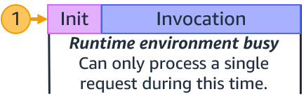
First request to invoke your function

At the first request to invoke your function, Lambda creates a new runtime environment. It then runs the function’s initialization (init) code, which is the code outside the main handler. Lambda then runs the function handler code as the invocation. This receives the event payload and processes your business logic.

Each runtime environment processes a single request at a time. While a single runtime environment is processing a request, it cannot process other requests.

After Lambda finishes processing the request, the runtime environment is ready to process an additional request for the same function. As the initialization code has already run, for request 2, Lambda runs only the function handler code as the invocation.

Lambda ready to process an additional request for the same function

If additional requests arrive while processing request 1, Lambda creates new runtime environments. In this example, Lambda creates new runtime environments for requests 2, 3, 4, and 5. It runs the function init and the invocation.

Lambda creating new runtime environments

When requests arrive, Lambda reuses available runtime environments, and creates new ones if necessary. The following example shows the behavior for additional requests after 1-5.

Lambda reusing runtime environments

Once request 1 completes, the runtime environment is available to process another request. When request 6 arrives, Lambda re-uses request 1s runtime environment and runs the invocation. This process continues for requests 7 and 8, which reuse the runtime environments from requests 2 and 3. When request 9 arrives, Lambda creates a new runtime environment as there isn’t an existing one available. When request 10 arrives, it reuses the runtime environment freed up after request 4.

The number of runtime environments determines the concurrency. This is the sum of all concurrent requests for currently running functions at a particular point in time. For a single runtime environment, the number of concurrent requests is 1.

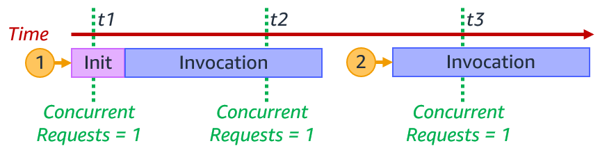
Single runtime environment concurrent requests

For the example with requests 1–10, the Lambda function concurrency at particular times is the following:

Lambda concurrency at particular times

time	concurrency
t1	3
t2	5
t3	4
t4	6
t5	5
t6	2

When the number of requests decreases, Lambda stops unused runtime environments to free up scaling capacity for other functions.

Invocation duration, concurrency, and transactions per second

The number of transactions Lambda can process per second is the sum of all invokes for that period. If a function takes 1 second to run, and 10 invocations happen concurrently, Lambda creates 10 runtime environments. In this case, Lambda processes 10 requests per second.

Lambda transactions per second for 1 second invocation

If the function duration is halved to 500 ms, the Lambda concurrency remains 10. However, transactions per second are now 20.

Lambda transactions per second for 500 ms second invocation

If the function takes 2 seconds to run, during the initial second, transactions per second is 0. However, averaged over time, transactions per second is 5.

You can view concurrency using Amazon CloudWatch metrics. Use the metric name ConcurrentExecutions to view concurrent invocations for all or individual functions.

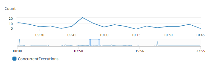
CloudWatch metrics ConcurrentExecutions

You can also estimate concurrent requests from the number of requests per unit of time, in this case seconds, and their average duration, using the formula:

RequestsPerSecond x AvgDurationInSeconds = concurrent requests

If a Lambda function takes an average 500 ms to run, at 100 requests per second, the number of concurrent requests is 50:

100 requests/second x 0.5 sec = 50 concurrent requests

If you half the function duration to 250 ms and the number of requests per second doubles to 200 requests/second, the number of concurrent requests remains the same:

200 requests/second x 0.250 sec = 50 concurrent requests.

Reducing a function’s duration can increase the transactions per second that a function can process. For more information on reducing function duration, watch this re:Invent video.

Scaling quotas

There are two scaling quotas to consider with concurrency. Account concurrency quota and burst concurrency quota.

Account concurrency is the maximum concurrency in a particular Region. This is shared across all functions in an account. The default Regional concurrency quota starts at 1,000, which you can increase with a service ticket.

The burst concurrency quota provides an initial burst of traffic for each function, between 500 and 3000 per minute, depending on the Region.

After this initial burst, functions can scale by another 500 concurrent invocations per minute for all Regions. If you reach the maximum number of concurrent requests, further requests are throttled.

For synchronous invocations, Lambda returns a throttling error (429) to the caller, which must retry the request. With asynchronous and event source mapping invokes, Lambda automatically retries the requests. See Error handling and automatic retries in AWS Lambda for more detail.

A scaling quota example

The following walks through how account and burst concurrency work for an example application.

Anticipating handling additional load, the application builders have raised account concurrency to 7,000. There are no other Lambda functions running in this account, so this function can use all available account concurrency.

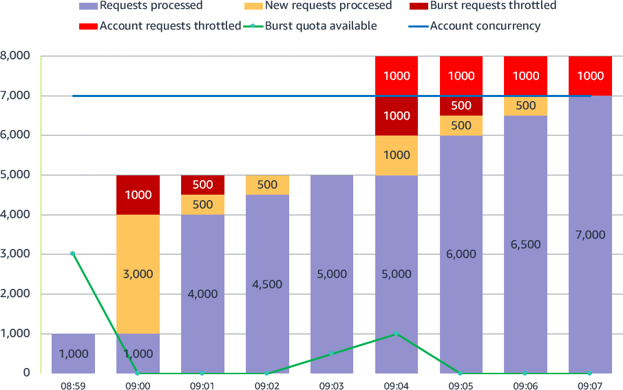
Lambda account and burst concurrency

08:59: The application already has a steady stream of requests, using 1,000 concurrent runtime environments. Each Lambda invocation takes 250 ms, so transactions per second are 4,000.
09:00: There is a large spike in traffic at 5,000 sustained requests. 1000 requests use the existing runtime environments. Lambda uses the 3,000 available burst concurrency to create new environments to handle the additional load. 1,000 requests are throttled as there is not enough burst concurrency to handle all 5,000 requests. Transactions per second are 16,000.
09:01: Lambda scales by another 500 concurrent invocations per minute. 500 requests are still throttled. The application can now handle 4,500 concurrent requests.
09:02: Lambda scales by another 500 concurrent invocations per minute. No requests are throttled. The application can now handle all 5,000 requests.
09:03: The application continues to handle the sustained 5000 requests. The burst concurrency quota rises to 500.
09:04: The application sees another spike in traffic, this time unexpected. 3,000 new sustained requests arrive, a combination of 8,000 requests. 5,000 requests use the existing runtime environments. Lambda uses the now available burst concurrency of 1,000 to create new environments to handle the additional load. 1,000 requests are throttled as there is not enough burst concurrency. Another 1,000 requests are throttled as the account concurrency quota has been reached.
09:05: Lambda scales by another 500 concurrent requests. The application can now handle 6,500 requests. 500 requests are throttled as there is not enough burst concurrency. 1,000 requests are still throttled as the account concurrency quota has been reached.
09:06: Lambda scales by another 500 concurrent requests. The application can now handle 7,000 requests. 1,000 requests are still throttled as the account concurrency quota has been reached.
09:07: The application continues to handle the sustained 7,000 requests. 1,000 requests are still throttled as the account concurrency quota has been reached. Transactions per second are 28,000.

Service Quotas is an AWS service that helps you manage your quotas for many AWS services. Along with looking up the values, you can also request a limit increase from the Service Quotas console.

Service Quotas console

Reserved concurrency

You can configure a Reserved concurrency setting for your Lambda functions to allocate a maximum concurrency limit for a function. This assigns part of the account concurrency quota to a specific function. This protects and ensures that a function is not throttled and can always scale up to the reserved concurrency value.

It can also help protect downstream resources. If a database or external API can only handle 2 concurrent connections, you can ensure Lambda can’t scale beyond 2 concurrent invokes. This ensures Lambda doesn’t overwhelm the downstream service. You can also use reserved concurrency to avoid race conditions to ensure that your function can only run one concurrent invocation at a time.

Reserved concurrency

You can also set the function concurrency to zero, which stops any function invocations and acts as an off-switch. This can be useful to stop Lambda invocations when you have an issue with a downstream resource. It can give you time to fix the issue before removing or increasing the concurrency to allow invocations to continue.

Provisioned Concurrency

The function initialization process can introduce latency for your applications. You can reduce this latency by configuring Provisioned Concurrency for a function version or alias. This prepares runtime environments in advance, running the function initialization process, so the function is ready to invoke when needed.

This is primarily useful for synchronous requests to ensure you have enough concurrency before an expected traffic spike. You can still burst above this using standard concurrency. The following example shows Provisioned Concurrency configured as 10. Lambda runs the init process for 10 functions, and then when requests arrive, immediately runs the invocation.

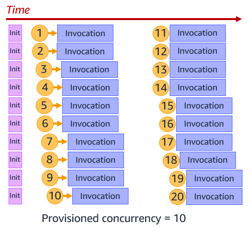
Provisioned Concurrency

You can use Application Auto Scaling to adjust Provisioned Concurrency automatically based on Lambda’s utilization metric.

Operational metrics

There are CloudWatch metrics available to monitor your account and function concurrency to ensure that your applications can scale as expected. Monitor function Invocations and Duration to understand throughput. Throttles show throttled invocations.

ConcurrentExecutions tracks the total number of runtime environments that are processing events. Ensure this doesn’t reach your account concurrency to avoid account throttling. Use the metric for individual functions to see which are using account concurrency, and also ensure reserved concurrency is not too high. For example, a function may have a reserved concurrency of 2000, but is only using 10.

UnreservedConcurrentExecutions show the number of function invocations without reserved concurrency. This is your available account concurrency buffer.

Use ProvisionedConcurrencyUtilization to ensure you are not paying for Provisioned Concurrency that you are not using. The metric shows the percentage of allocated Provisioned Concurrency in use.

ProvisionedConcurrencySpilloverInvocations show function invocations using standard concurrency, above the configured Provisioned Concurrency value. This may show that you need to increase Provisioned Concurrency.

Conclusion

Lambda provides a highly scalable compute service. Understanding how Lambda scaling and throughput works can help you design your application, especially for high load.

This post explains concurrency and transactions per second. It shows how account and burst concurrency quotas work. You can configure reserved concurrency to ensure that your functions can always scale, and also use it to protect downstream resources. Use Provisioned Concurrency to scale up Lambda in advance of invokes.

For more serverless learning resources, visit Serverless Land.

A story about AF_XDP, network namespaces and a cookie

2022-07-18 Bastien Dhiver

Post Syndicated from Bastien Dhiver original https://blog.cloudflare.com/a-story-about-af-xdp-network-namespaces-and-a-cookie/

A story about AF_XDP, network namespaces and a cookie

A crash in a development version of flowtrackd (the daemon that powers our Advanced TCP Protection) highlighted the fact that libxdp (and specifically the AF_XDP part) was not Linux network namespace aware.

This blogpost describes the debugging journey to find the bug, as well as a fix.

flowtrackd is a volumetric denial of service defense mechanism that sits in the Magic Transit customer’s data path and protects the network from complex randomized TCP floods. It does so by challenging TCP connection establishments and by verifying that TCP packets make sense in an ongoing flow.

It uses the Linux kernel AF_XDP feature to transfer packets from a network device in kernel space to a memory buffer in user space without going through the network stack. We use most of the helper functions of the C libbpf with the Rust bindings to interact with AF_XDP.

In our setup, both the ingress and the egress network interfaces are in different network namespaces. When a packet is determined to be valid (after a challenge or under some thresholds), it is forwarded to the second network interface.

For the rest of this post the network setup will be the following:

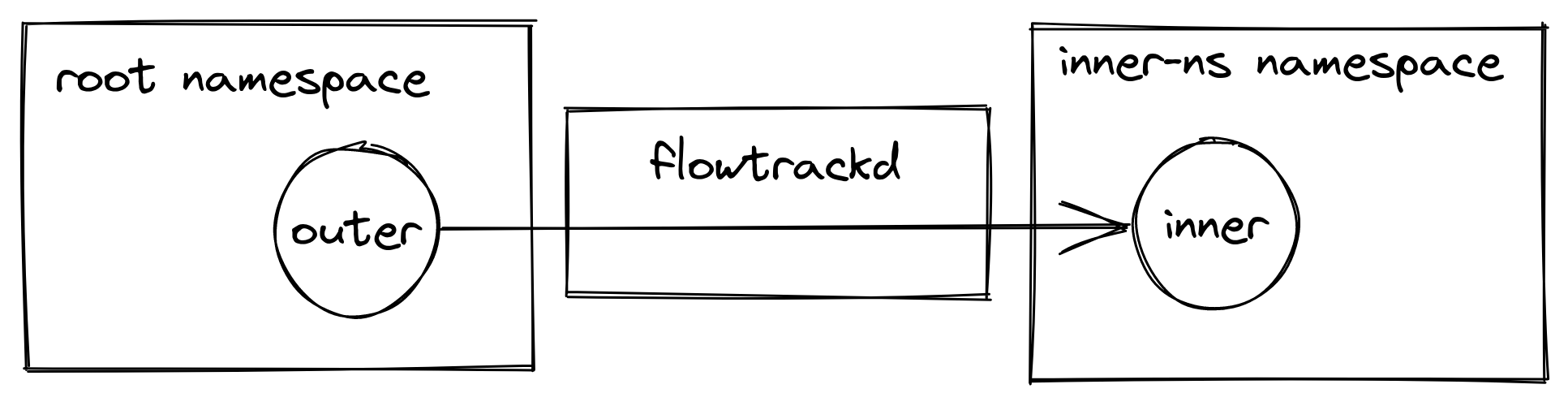
e.g. eyeball packets arrive at the outer device in the root network namespace, they are picked up by flowtrackd and then forwarded to the inner device in the inner-ns namespace.

AF_XDP

The kernel and the userspace share a memory buffer called the UMEM. This is where packet bytes are written to and read from.

The UMEM is split in contiguous equal-sized “frames” that are referenced by “descriptors” which are just offsets from the start address of the UMEM.

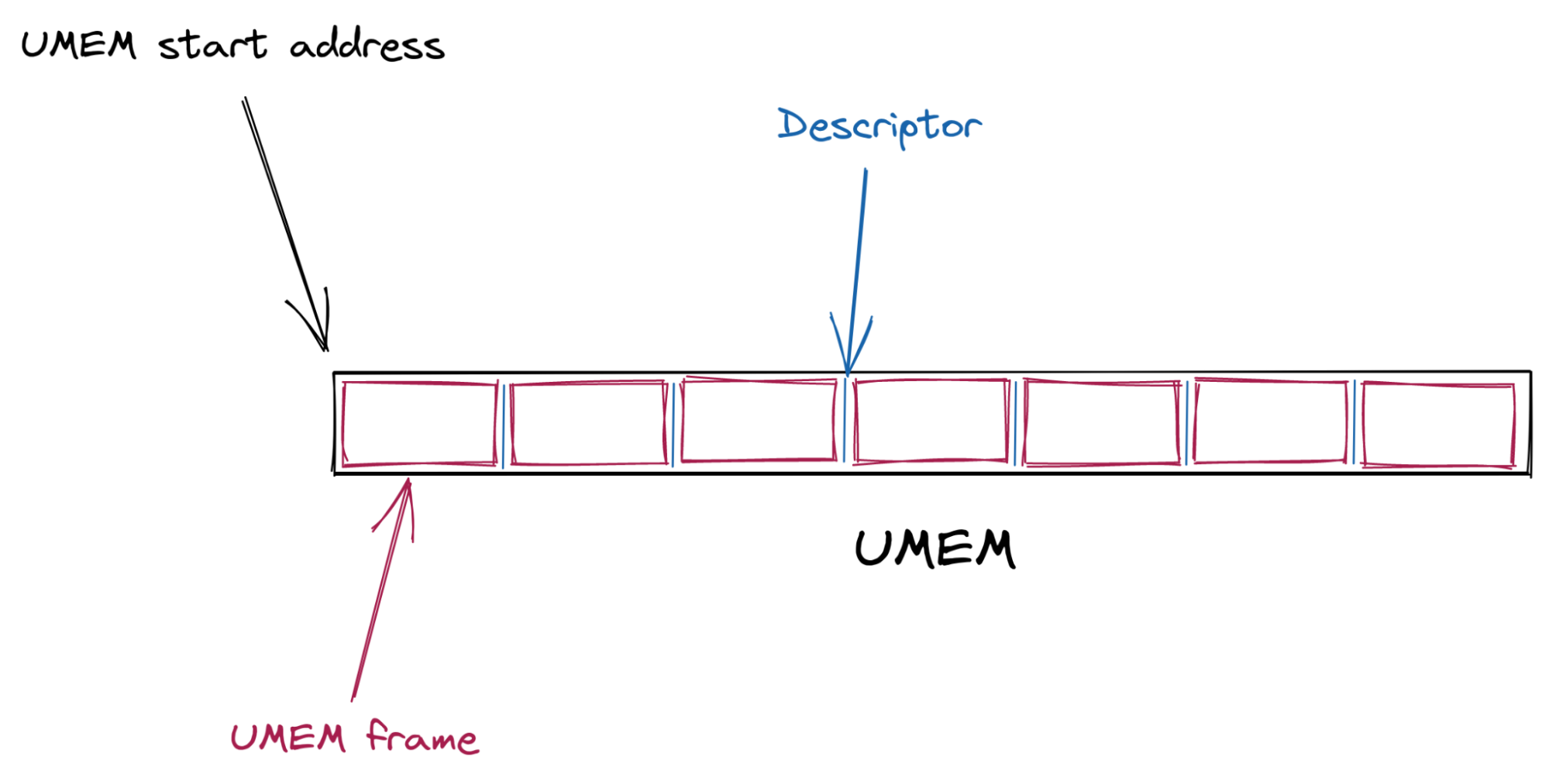
The interactions and synchronization between the kernel and userspace happen via a set of queues (circular buffers) as well as a socket from the AF_XDP family.

Most of the work is about managing the ownership of the descriptors. Which descriptors the kernel owns and which descriptors the userspace owns.

The interface provided for the ownership management are a set of queues:

Queue	User space	Kernel space	Content description
COMPLETION	Consumes	Produces	Frame descriptors that have successfully been transmitted
FILL	Produces	Consumes	Frame descriptors ready to get new packet bytes written to
RX	Consumes	Produces	Frame descriptors of a newly received packet
TX	Produces	Consumes	Frame descriptors to be transmitted

When the UMEM is created, a FILL and a COMPLETION queue are associated with it.

An RX and a TX queue are associated with the AF_XDP socket (abbreviated Xsk) at its creation. This particular socket is bound to a network device queue id. The userspace can then poll() on the socket to know when new descriptors are ready to be consumed from the RX queue and to let the kernel deal with the descriptors that were set on the TX queue by the application.

The last plumbing operation to be done to use AF_XDP is to load a BPF program attached with XDP on the network device we want to interact with and insert the Xsk file descriptor into a BPF map (of type XSKMAP). Doing so will enable the BPF program to redirect incoming packets (with the bpf_redirect_map() function) to a specific socket that we created in userspace:

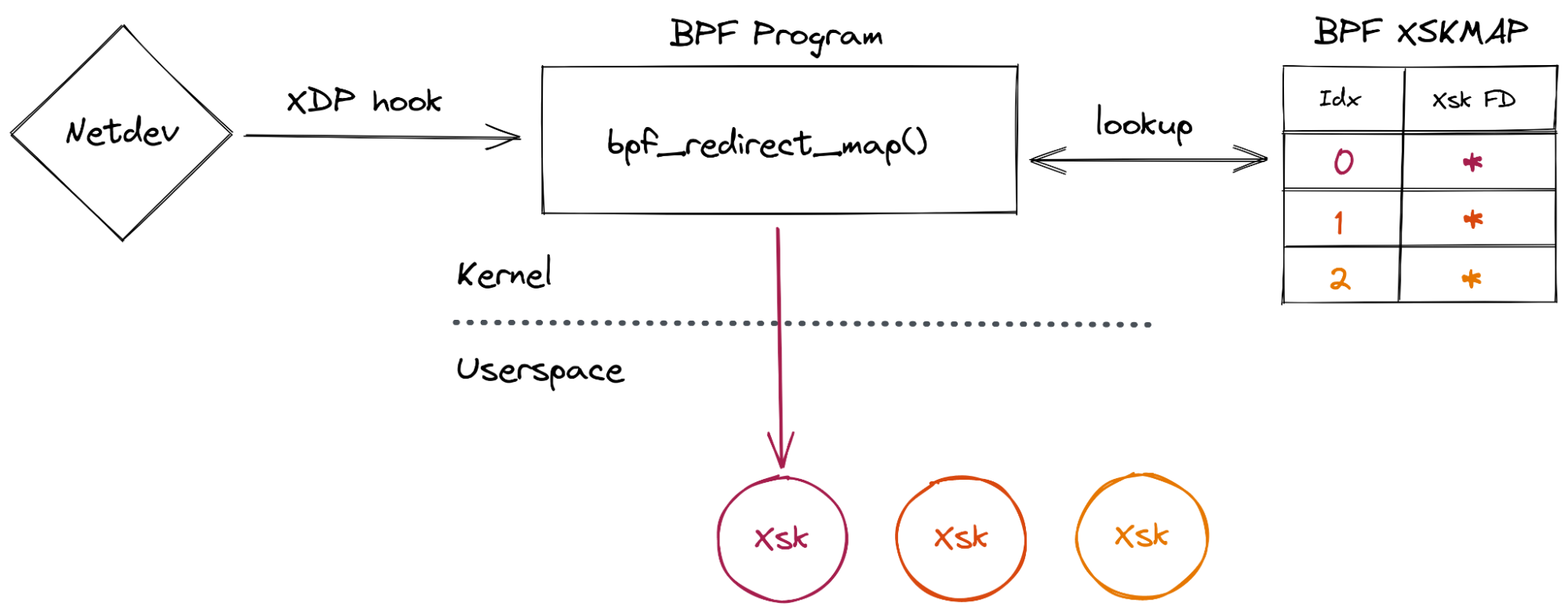
Once everything has been allocated and strapped together, what I call “the descriptors dance” can start. While this has nothing to do with courtship behaviors it still requires a flawless execution:

When the kernel receives a packet (more specifically the device driver), it will write the packet bytes to a UMEM frame (from a descriptor that the userspace put in the FILL queue) and then insert the frame descriptor in the RX queue for the userspace to consume. The userspace can then read the packet bytes from the received descriptor, take a decision, and potentially send it back to the kernel for transmission by inserting the descriptor in the TX queue. The kernel can then transmit the content of the frame and put the descriptor from the TX to the COMPLETION queue. The userspace can then “recycle” this descriptor in the FILL or TX queue.

The overview of the queue interactions from the application perspective is represented on the following diagram (note that the queues contain descriptors that point to UMEM frames):

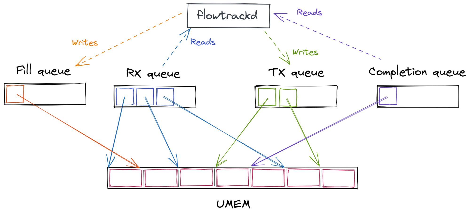
flowtrackd I/O rewrite project

To increase flowtrackd performance and to be able to scale with the growth of the Magic Transit product we decided to rewrite the I/O subsystem.

There will be a public blogpost about the technical aspects of the rewrite.

Prior to the rewrite, each customer had a dedicated flowtrackd instance (Unix process) that attached itself to dedicated network devices. A dedicated UMEM was created per network device (see schema on the left side below). The packets were copied from one UMEM to the other.

In this blogpost, we will only focus on the new usage of the AF_XDP shared UMEM feature which enables us to handle all customer accounts with a single flowtrackd instance per server and with a single shared UMEM (see schema on the right side below).

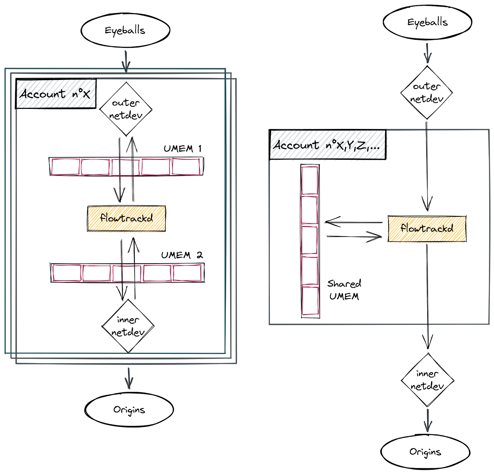
The Linux kernel documentation describes the additional plumbing steps to share a UMEM across multiple AF_XDP sockets:

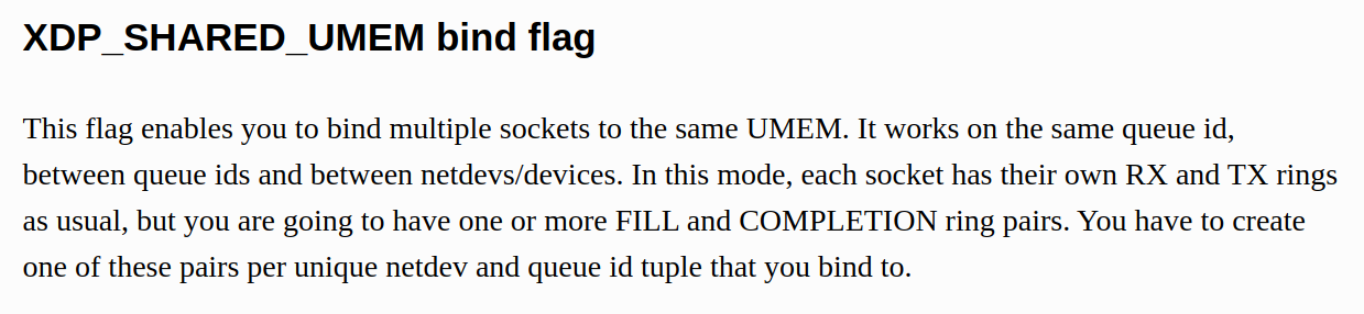
Followed by the instructions for our use case:

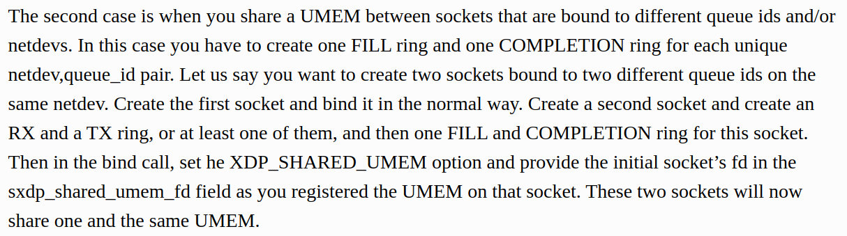
Hopefully for us a helper function in libbpf does it all for us: xsk_socket__create_shared()

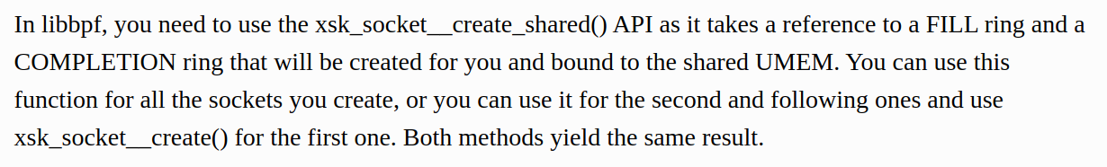
The final setup is the following: Xsks are created for each queue of the devices in their respective network namespaces. flowtrackd then handles the descriptors like a puppeteer while applying our DoS mitigation logic on the packets that they reference with one exception… (notice the red crosses on the diagram):

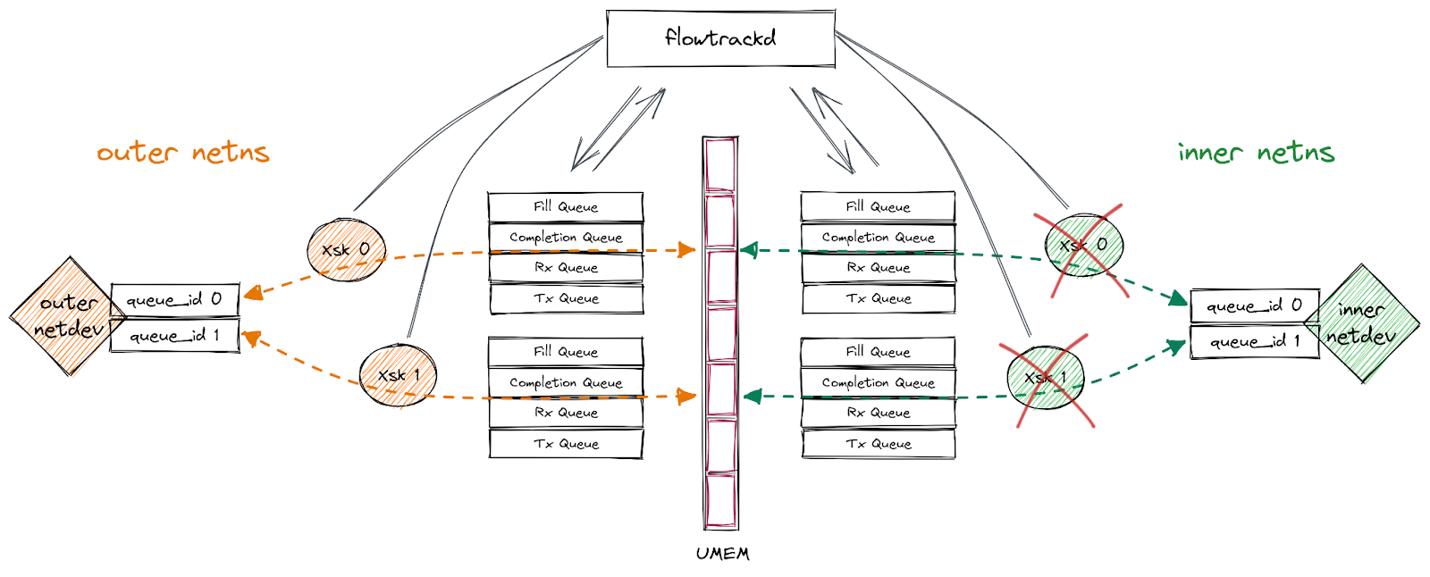
What “Invalid argument” ??!

We were happily near the end of the rewrite when, suddenly, after porting our integration tests in the CI, flowtrackd crashed!

The following errors was displayed:

[...]
Thread 'main' panicked at 'failed to create Xsk: Libbpf("Invalid argument")', flowtrack-io/src/packet_driver.rs:144:22
note: run with `RUST_BACKTRACE=1` environment variable to display a backtrace

According to the line number, the first socket was created with success and flowtrackd crashed when the second Xsk was created:

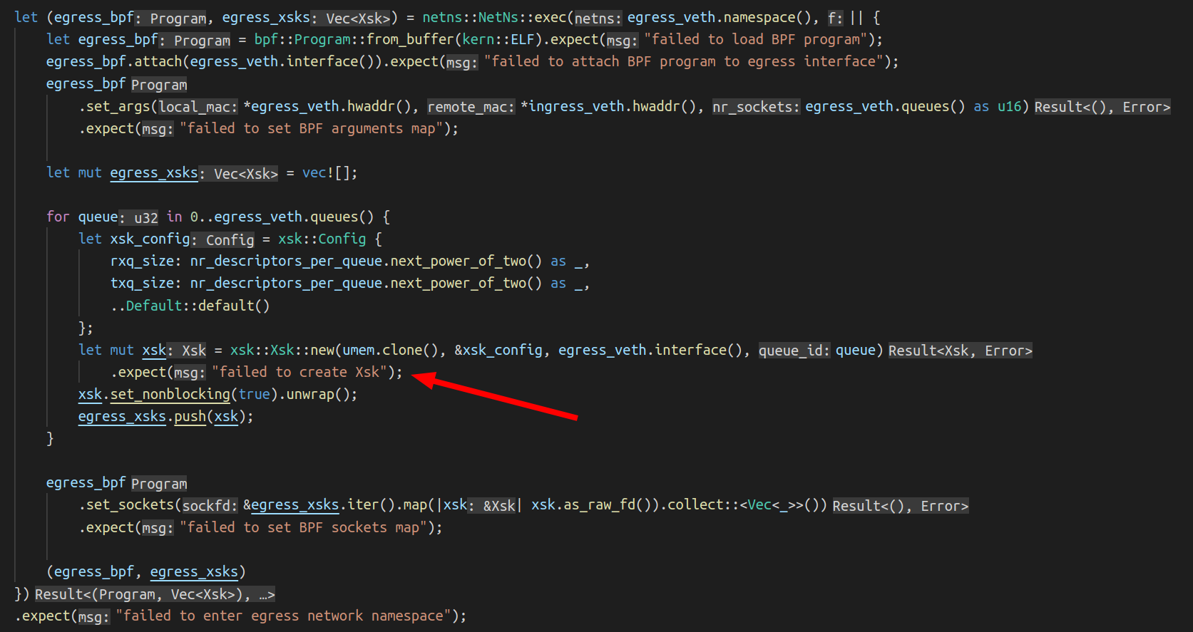
Here is what we do: we enter the network namespace where the interface sits, load and attach the BPF program and for each queue of the interface, we create a socket. The UMEM and the config parameters are the same with the ingress Xsk creation. Only the ingress_veth and egress_veth are different.

This is what the code to create an Xsk looks like:

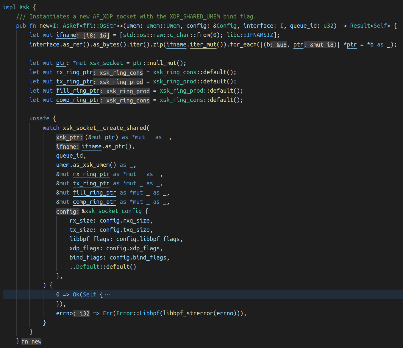
The call to the libbpf function xsk_socket__create_shared() didn’t return 0.

The libxdp manual page doesn’t help us here…

Which argument is “invalid”? And why is this error not showing up when we run flowtrackd locally but only in the CI?

We can try to reproduce locally with a similar network setup script used in the CI:

#!/bin/bash
 
set -e -u -x -o pipefail
 
OUTER_VETH=${OUTER_VETH:=outer}
TEST_NAMESPACE=${TEST_NAMESPACE:=inner-ns}
INNER_VETH=${INNER_VETH:=inner}
QUEUES=${QUEUES:=$(grep -c ^processor /proc/cpuinfo)}
 
ip link delete $OUTER_VETH &>/dev/null || true
ip netns delete $TEST_NAMESPACE &>/dev/null || true
ip netns add $TEST_NAMESPACE
ip link \
  add name $OUTER_VETH numrxqueues $QUEUES numtxqueues $QUEUES type veth \
  peer name $INNER_VETH netns $TEST_NAMESPACE numrxqueues $QUEUES numtxqueues $QUEUES
ethtool -K $OUTER_VETH tx off rxvlan off txvlan off
ip link set dev $OUTER_VETH up
ip addr add 169.254.0.1/30 dev $OUTER_VETH
ip netns exec $TEST_NAMESPACE ip link set dev lo up
ip netns exec $TEST_NAMESPACE ethtool -K $INNER_VETH tx off rxvlan off txvlan off
ip netns exec $TEST_NAMESPACE ip link set dev $INNER_VETH up
ip netns exec $TEST_NAMESPACE ip addr add 169.254.0.2/30 dev $INNER_VETH

For the rest of the blogpost, we set the number of queues per interface to 1. If you have questions about the set command in the script, check this out.

Not much success triggering the error.

What differs between my laptop setup and the CI setup?

I managed to find out that when the outer and inner interface index numbers are the same then it crashes. Even though the interfaces don’t have the same name, and they are not in the same network namespace. When the tests are run by the CI, both interfaces got index number 5 which was not the case on my laptop since I have more interfaces:

$ ip -o link | cut -d' ' -f1,2
1: lo:
2: wwan0:
3: wlo1:
4: virbr0:
7: br-ead14016a14c:
8: docker0:
9: br-bafd94c79ff4:
29: outer@if2:

We can edit the script to set a fixed interface index number:

ip link \
  add name $OUTER_VETH numrxqueues $QUEUES numtxqueues $QUEUES index 4242 type veth \
  peer name $INNER_VETH netns $TEST_NAMESPACE numrxqueues $QUEUES numtxqueues $QUEUES index 4242

And we can now reproduce the issue locally!

Interesting observation: I was not able to reproduce this issue with the previous flowtrackd version. Is this somehow related to the shared UMEM feature that we are now using?

Back to the “invalid” argument. strace to the rescue:

sudo strace -f -x ./flowtrackd -v -c flowtrackd.toml --ingress outer --egress inner --egress-netns inner-ns
 
[...]
 
// UMEM allocation + first Xsk creation
 
[pid 389577] brk(0x55b485819000)        = 0x55b485819000
[pid 389577] mmap(NULL, 8396800, PROT_READ|PROT_WRITE, MAP_PRIVATE|MAP_ANONYMOUS, -1, 0) = 0x7f85037fe000
 
[pid 389577] socket(AF_XDP, SOCK_RAW|SOCK_CLOEXEC, 0) = 9
[pid 389577] setsockopt(9, SOL_XDP, XDP_UMEM_REG, "\x00\xf0\x7f\x03\x85\x7f\x00\x00\x00\x00\x80\x00\x00\x00\x00\x00\x00\x08\x00\x00\x00\x00\x00\x00\x00\x00\x00\x00\x00\x00\x00\x00", 32) = 0
[pid 389577] setsockopt(9, SOL_XDP, XDP_UMEM_FILL_RING, [2048], 4) = 0
[pid 389577] setsockopt(9, SOL_XDP, XDP_UMEM_COMPLETION_RING, [2048], 4) = 0
[pid 389577] getsockopt(9, SOL_XDP, XDP_MMAP_OFFSETS, "\x00\x00\x00\x00\x00\x00\x00\x00\x80\x00\x00\x00\x00\x00\x00\x00\x40\x01\x00\x00\x00\x00\x00\x00\xc4\x00\x00\x00\x00\x00\x00\x00"..., [128]) = 0
[pid 389577] mmap(NULL, 16704, PROT_READ|PROT_WRITE, MAP_SHARED|MAP_POPULATE, 9, 0x100000000) = 0x7f852801b000
[pid 389577] mmap(NULL, 16704, PROT_READ|PROT_WRITE, MAP_SHARED|MAP_POPULATE, 9, 0x180000000) = 0x7f8528016000
[...]
[pid 389577] setsockopt(9, SOL_XDP, XDP_RX_RING, [2048], 4) = 0
[pid 389577] setsockopt(9, SOL_XDP, XDP_TX_RING, [2048], 4) = 0
[pid 389577] getsockopt(9, SOL_XDP, XDP_MMAP_OFFSETS, "\x00\x00\x00\x00\x00\x00\x00\x00\x80\x00\x00\x00\x00\x00\x00\x00\x40\x01\x00\x00\x00\x00\x00\x00\xc4\x00\x00\x00\x00\x00\x00\x00"..., [128]) = 0
[pid 389577] mmap(NULL, 33088, PROT_READ|PROT_WRITE, MAP_SHARED|MAP_POPULATE, 9, 0) = 0x7f850377e000
[pid 389577] mmap(NULL, 33088, PROT_READ|PROT_WRITE, MAP_SHARED|MAP_POPULATE, 9, 0x80000000) = 0x7f8503775000
[pid 389577] bind(9, {sa_family=AF_XDP, sa_data="\x08\x00\x92\x10\x00\x00\x00\x00\x00\x00\x00\x00\x00\x00"}, 16) = 0
 
[...]
 
// Second Xsk creation
 
[pid 389577] socket(AF_XDP, SOCK_RAW|SOCK_CLOEXEC, 0) = 62
[...]
[pid 389577] setsockopt(62, SOL_XDP, XDP_RX_RING, [2048], 4) = 0
[pid 389577] setsockopt(62, SOL_XDP, XDP_TX_RING, [2048], 4) = 0
[pid 389577] getsockopt(62, SOL_XDP, XDP_MMAP_OFFSETS, "\x00\x00\x00\x00\x00\x00\x00\x00\x80\x00\x00\x00\x00\x00\x00\x00\x40\x01\x00\x00\x00\x00\x00\x00\xc4\x00\x00\x00\x00\x00\x00\x00"..., [128]) = 0
[pid 389577] mmap(NULL, 33088, PROT_READ|PROT_WRITE, MAP_SHARED|MAP_POPULATE, 62, 0) = 0x7f85036e4000
[pid 389577] mmap(NULL, 33088, PROT_READ|PROT_WRITE, MAP_SHARED|MAP_POPULATE, 62, 0x80000000) = 0x7f85036db000
[pid 389577] bind(62, {sa_family=AF_XDP, sa_data="\x01\x00\x92\x10\x00\x00\x00\x00\x00\x00\x09\x00\x00\x00"}, 16) = -1 EINVAL (Invalid argument)
 
[pid 389577] munmap(0x7f85036db000, 33088) = 0
[pid 389577] munmap(0x7f85036e4000, 33088) = 0
[pid 389577] close(62)                  = 0
[pid 389577] write(2, "thread '", 8thread ')    = 8
[pid 389577] write(2, "main", 4main)        = 4
[pid 389577] write(2, "' panicked at '", 15' panicked at ') = 15
[pid 389577] write(2, "failed to create Xsk: Libbpf(\"In"..., 48failed to create Xsk: Libbpf("Invalid argument")) = 48
[...]

Ok, the second bind() syscall returns the EINVAL value.

The sa_family is the right one. Is something wrong with sa_data="\x01\x00\x92\x10\x00\x00\x00\x00\x00\x00\x09\x00\x00\x00" ?

Let’s look at the bind syscall kernel code:

err = sock->ops->bind(sock, (struct sockaddr *) &address, addrlen);

The bind function of the protocol specific socket operations gets called. Searching for “AF_XDP” in the code, we quickly found the bind function call related to the AF_XDP socket address family.

So, where in the syscall could this value be returned?

First, let’s examine the syscall parameters to see if the libbpf xsk_socket__create_shared() function sets weird values for us.

We use the pahole tool to print the structure definitions:

$ pahole sockaddr
struct sockaddr {
        sa_family_t                sa_family;            /*     0     2 */
        char                       sa_data[14];          /*     2    14 */
 
        /* size: 16, cachelines: 1, members: 2 */
        /* last cacheline: 16 bytes */
};
 
$ pahole sockaddr_xdp
struct sockaddr_xdp {
        __u16                      sxdp_family;          /*     0     2 */
        __u16                      sxdp_flags;           /*     2     2 */
        __u32                      sxdp_ifindex;         /*     4     4 */
        __u32                      sxdp_queue_id;        /*     8     4 */
        __u32                      sxdp_shared_umem_fd;  /*    12     4 */
 
        /* size: 16, cachelines: 1, members: 5 */
        /* last cacheline: 16 bytes */
};

Translation of the arguments of the bind syscall (the 14 bytes of sa_data) for the first bind() call:

Struct member	Big Endian value	Decimal	Meaning	Observation
sxdp_flags	\x08\x00	8	XDP_USE_NEED_WAKEUP	expected
sxdp_ifindex	\x92\x10\x00\x00	4242	The network interface index	expected
sxdp_queue_id	\x00\x00\x00\x00	0	The network interface queue id	expected
sxdp_shared_umem_fd	\x00\x00\x00\x00	0	The umem is not shared yet	expected

Second bind() call:

Struct member	Big Endian value	Decimal	Meaning	Observation
sxdp_flags	\x01\x00	1	XDP_SHARED_UMEM	expected
sxdp_ifindex	\x92\x10\x00\x00	4242	The network interface index	expected
sxdp_queue_id	\x00\x00\x00\x00	0	The network interface queue id	expected
sxdp_shared_umem_fd	\x09\x00\x00\x00	9	File descriptor of the first AF_XDP socket associated to the UMEM	expected

The arguments look good…

We could statically try to infer where the EINVAL was returned looking at the source code. But this analysis has its limits and can be error-prone.

Overall, it seems that the network namespaces are not taken into account somewhere because it seems that there is some confusion with the interface indexes.

Is the issue on the kernel-side?

Digging deeper

It would be nice if we had step-by-step runtime inspection of code paths and variables.

Let’s:

Compile a Linux kernel version closer to the one used on our servers (5.15) with debug symbols.
Generate a root filesystem for the kernel to boot.
Boot in QEMU.
Attach gdb to it and set a breakpoint on the syscall.
Check where the EINVAL value is returned.

We could have used buildroot with a minimal reproduction code, but it wasn’t funny enough. Instead, we install a minimal Ubuntu and load our custom kernel. This has the benefit of having a package manager if we need to install other debugging tools.

Let’s install a minimal Ubuntu server 21.10 (with ext4, no LVM and a ssh server selected in the installation wizard):

qemu-img create -f qcow2 ubuntu-21.10-live-server-amd64.qcow2 20G
 
qemu-system-x86_64 \
  -smp $(nproc) \
  -m 4G \
  -hda ubuntu-21.10-live-server-amd64.qcow2 \
  -cdrom /home/bastien/Downloads/ubuntu-21.10-live-server-amd64.iso \
  -enable-kvm \
  -cpu host \
  -net nic,model=virtio \
  -net user,hostfwd=tcp::10022-:22

And then build a kernel (link and link) with the following changes in the menuconfig:

Cryptographic API -> Certificates for signature checking -> Provide system-wide ring of trusted keys
- change the additional string to be EMPTY ("")
Device drivers -> Network device support -> Virtio network driver
- Set to Enable
Device Drivers -> Network device support -> Virtual ethernet pair device
- Set to Enable
Device drivers -> Block devices -> Virtio block driver
- Set to Enable

git clone git://git.kernel.org/pub/scm/linux/kernel/git/stable/linux.git && cd linux/
git checkout v5.15
make menuconfig
make -j$(nproc) bzImage

We can now run Ubuntu with our custom kernel waiting for gdb to be connected:

qemu-system-x86_64 \
  -kernel /home/bastien/work/linux/arch/x86_64/boot/bzImage \
  -append "root=/dev/sda2 console=ttyS0 nokaslr" \
  -nographic \
  -smp $(nproc) \
  -m 8G \
  -hda ubuntu-21.10-live-server-amd64.qcow2 \
  -boot c \
  -cpu host \
  -net nic,model=virtio \
  -net user,hostfwd=tcp::10022-:22 \
  -enable-kvm \
  -s -S

And we can fire up gdb and set a breakpoint on the xsk_bind function:

$ gdb  -ex "add-auto-load-safe-path $(pwd)" -ex "file vmlinux" -ex "target remote :1234" -ex "hbreak start_kernel" -ex "continue"
(gdb) b xsk_bind
(gdb) continue

After executing the network setup script and running flowtrackd, we hit the xsk_bind breakpoint:

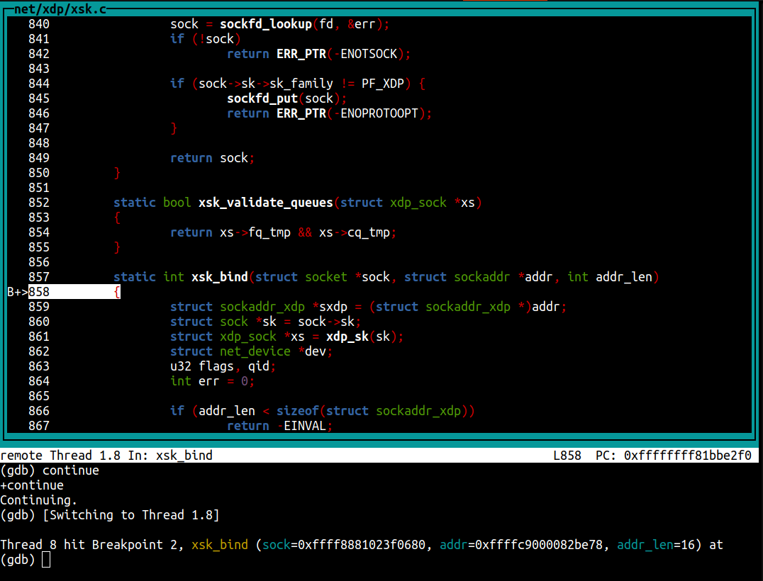
We continue to hit the second xsk_bind breakpoint (the one that returns EINVAL) and after a few next and step commands, we find which function returned the EINVAL value:

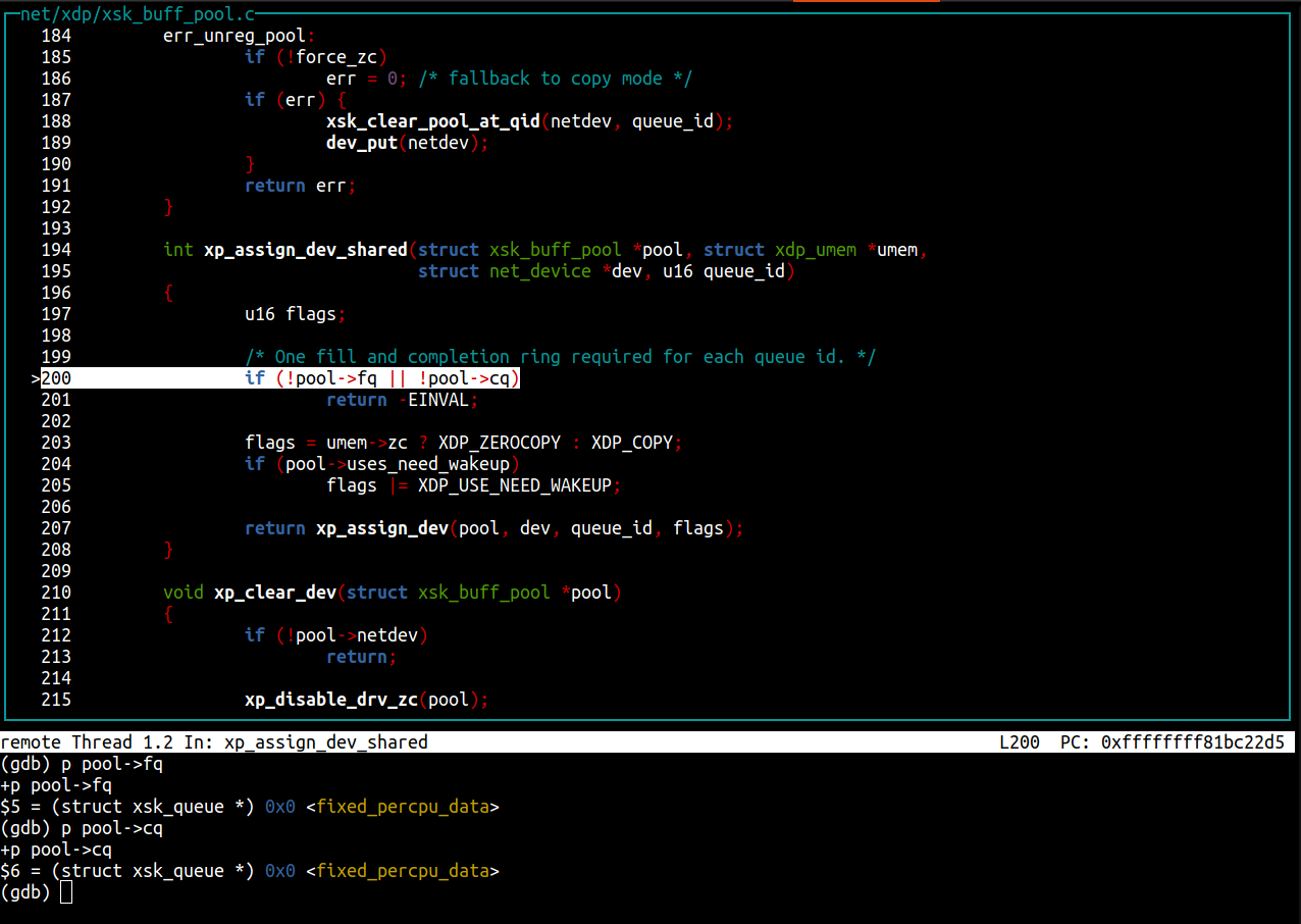
In our Rust code, we allocate a new FILL and a COMPLETION queue for each queue id of the device prior to calling xsk_socket__create_shared(). Why are those set to NULL? Looking at the code, pool->fq comes from a struct field named fq_tmp that is accessed from the sock pointer (print ((struct xdp_sock *)sock->sk)->fq_tmp). The field is set in the first call to xsk_bind() but isn’t in the second call. We note that at the end of the xsk_bind() function, fq_tmp and cq_tmp are set to NULL as per this comment: “FQ and CQ are now owned by the buffer pool and cleaned up with it.”.

Something is definitely going wrong in libbpf because the FILL queue and COMPLETION queue pointers are missing.

Back to the libbpf xsk_socket__create_shared() function to check where the queues are set for the socket and we quickly notice two functions that interact with the FILL and COMPLETION queues:

The first function called is xsk_get_ctx():

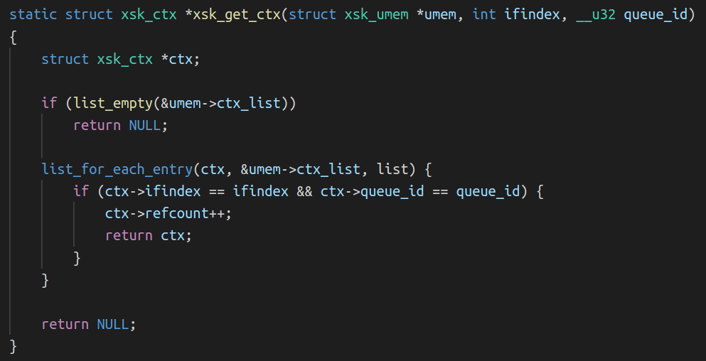
The second is xsk_create_ctx():

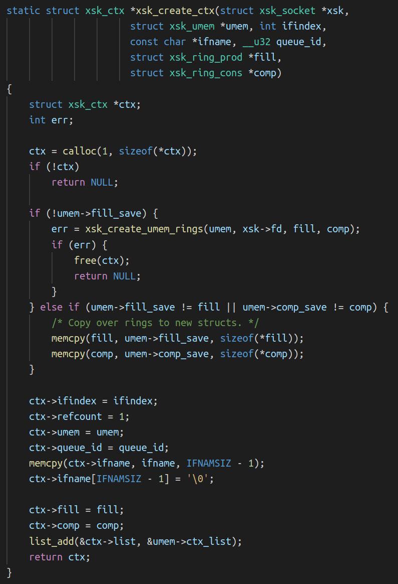
Remembering our setup, can you spot what the issue is?

The bug / missing feature

The issue is in the comparison performed in the xsk_get_ctx() to find the right socket context structure associated with the (ifindex, queue_id) pair in the linked-list. The UMEM being shared across Xsks, the same umem->ctx_list linked list head is used to find the sockets that use this UMEM. Remember that in our setup, flowtrackd attaches itself to two network devices that live in different network namespaces. Using the interface index and the queue_id to find the right context (FILL and COMPLETION queues) associated to a socket is not sufficient because another network interface with the same interface index can exist at the same time in another network namespace.

What can we do about it?

We need to tell apart two network devices “system-wide”. That means across the network namespace boundaries.

Could we fetch and store the network namespace inode number of the current process (stat -c%i -L /proc/self/ns/net) at the context creation and then use it in the comparison? According to man 7 inode: “Each file in a filesystem has a unique inode number. Inode numbers are guaranteed to be unique only within a filesystem”. However, inode numbers can be reused:

# ip netns add a
# stat -c%i /run/netns/a
4026532570
# ip netns delete a
# ip netns add b
# stat -c%i /run/netns/b
4026532570

Here are our options:

Do a quick hack to ensure that the interface indexes are not the same (as done in the integration tests).
Explain our use case to the libbpf maintainers and see how the API for the xsk_socket__create_shared() function should change. It could be possible to pass an opaque “cookie” as a parameter at the socket creation and pass it to the functions that access the socket contexts.
Take our chances and look for Linux patches that contain the words “netns” and “cookie”

Well, well, well: [PATCH bpf-next 3/7] bpf: add netns cookie and enable it for bpf cgroup hooks

This is almost what we need! This patch adds a kernel function named bpf_get_netns_cookie() that would get us the network namespace cookie linked to a socket:

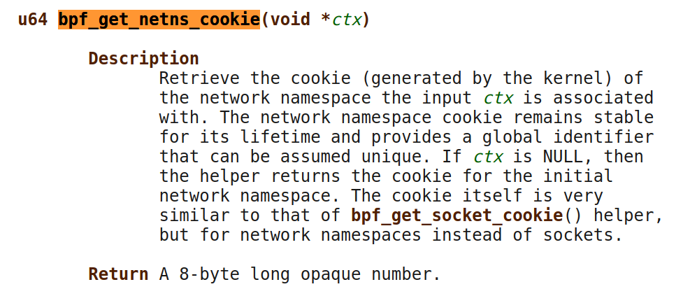
A second patch enables us to get this cookie from userspace:

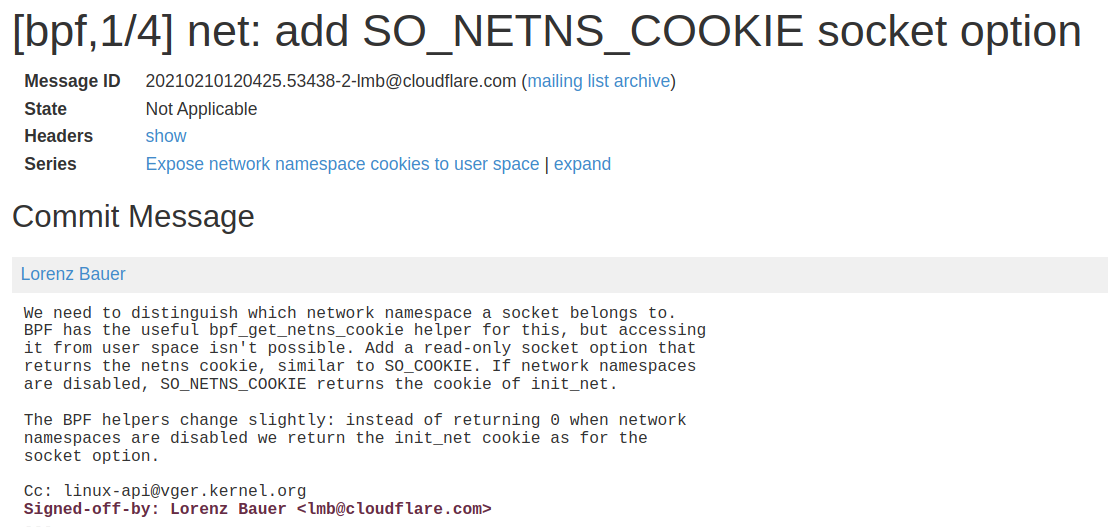
I know this Lorenz from somewhere 😀

Note that this patch was shipped with the Linux v5.14 release.

We have more guaranties now:

The cookie is generated for us by the kernel.
There is a strong bound to the socket from its creation (the netns cookie value is present in the socket structure).
The network namespace cookie remains stable for its lifetime.
It provides a global identifier that can be assumed unique and not reused.

A patch

At the socket creation, we retrieve the netns_cookie from the Xsk file descriptor with getsockopt(), insert it in the xsk_ctx struct and add it in the comparison performed in xsk_get_ctx().

Our initial patch was tested on Linux v5.15 with libbpf v0.8.0.

Testing the patch

We keep the same network setup script, but we set the number of queues per interface to two (QUEUES=2). This will help us check that two sockets created in the same network namespace have the same netns_cookie.

After recompiling flowtrackd to use our patched libbpf, we can run it inside our guest with gdb and set breakpoints on xsk_get_ctx as well as xsk_create_ctx. We now have two instances of gdb running at the same time, one debugging the system and the other debugging the application running in that system. Here is the gdb guest view:

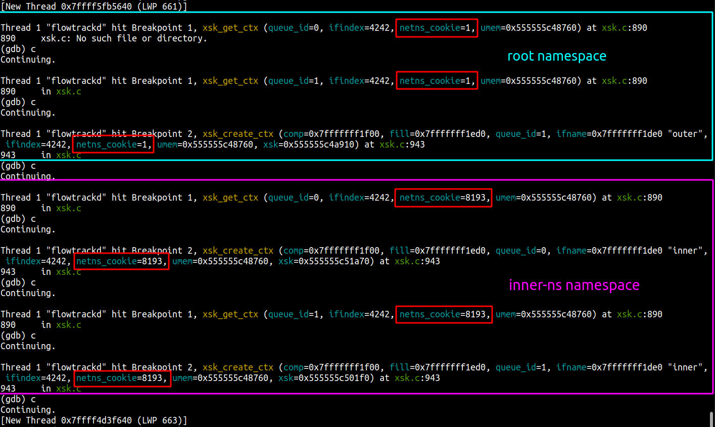
Here is the gdb system view:

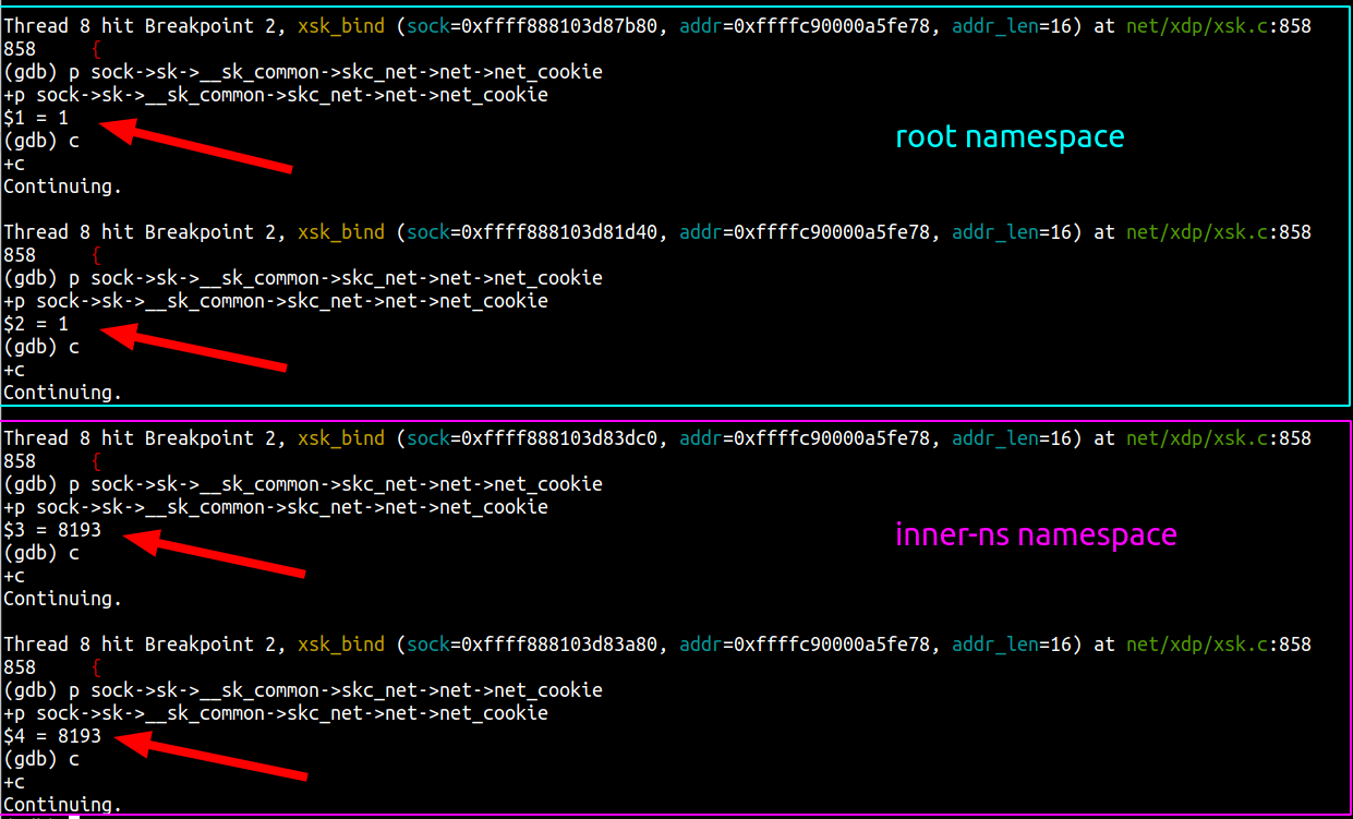
We can see that the netns_cookie value for the first two Xsks is 1 (root namespace) and the net_cookie value for the two other Xsks is 8193 (inner-ns namespace).

flowtrackd didn’t crash and is behaving as expected. It works!

Conclusion

Situation

Creating AF_XDP sockets with the XDP_SHARED_UMEM flag set fails when the two devices’ ifindex (and the queue_id) are the same. This can happen with devices in different network namespaces.

In the shared UMEM mode, each Xsk is expected to have a dedicated fill and completion queue. Context data about those queues are set by libbpf in a linked-list stored by the UMEM object. The comparison performed to pick the right context in the linked-list only takes into account the device ifindex and the queue_id which can be the same when devices are in different network namespaces.

Resolution

We retrieve the netns_cookie associated with the socket at its creation and add it in the comparison operation.

The fix has been submitted and merged in libxdp which is where the AF_XDP parts of libbpf now live.

We’ve also backported the fix in libbpf and updated the libbpf-sys Rust crate accordingly.

New York’s Secret Subway

2022-07-18 The History Guy: History Deserves to Be Remembered

Post Syndicated from The History Guy: History Deserves to Be Remembered original https://www.youtube.com/watch?v=rMf6KYhlRmg

Capri Suns

2022-07-18

Post Syndicated from original https://xkcd.com/2647/

[As security is dragging me away] "Come on, at least I didn't make the mistake in the other direction!"

Kernel prepatch 5.19-rc7

2022-07-18

Post Syndicated from original https://lwn.net/Articles/901581/

The 5.19-rc7 kernel prepatch is out for
testing.

We obviously had that whole “Retbleed” thing, and it does show up
in both the diffstat and the shortlog, and rc7 is definitely bigger
than usual. And also as usual, when we’ve had one of those
embargoed hw issues pending, the patches didn’t get the open
development, and then as a result missed all the usual sanity
checking by all the automation build and test infrastructure we
have. So no surprise – there’s been various small fixup patches
afterwards too for some corner cases.

That said, last week there were two other development trees that
independently also asked for an extension, so 5.19 will be one of
those releases that have an additional rc8 next weekend before the
final release.