FOSDEM’s organizers have announced
that all of the video recordings “worth publishing” from FOSDEM 2026 are now available.
Videos are linked from the individual schedule pages for the talks and
the full
schedule page. They are also available, organised by room, at video.fosdem.org/2026.
In the first quarter of 2026, government-directed shutdowns figured prominently, with prolonged Internet blackouts in both Uganda and Iran, a stark contrast to the lack of observed government-directed shutdowns in the same quarter a year prior. This quarter, we also observed a number of Internet disruptions caused by power outages, including three separate collapses of Cuba’s national electrical grid. Military action continued to disrupt connectivity in Ukraine and also impacted hyperscaler cloud infrastructure in the Middle East. Severe weather knocked out Internet connectivity in Portugal, while cable damage disrupted connectivity in the Republic of Congo. A technical problem hit Verizon Wireless in the United States, and unknown issues briefly disrupted connectivity for customers of providers in Guinea and the United Kingdom.
This post is intended as a summary overview of observed and confirmed disruptions and is not an exhaustive or complete list of issues that have occurred during the quarter. A larger list of detected traffic anomalies is available in the Cloudflare Radar Outage Center. Note that both bytes-based and request-based traffic graphs are used within this post to illustrate the impact of the observed disruptions, with the choice of metric generally made based on which better illustrates the impact of the disruption.
Government-directed shutdowns
Uganda
In advance of the January 15 presidential election, Ugandan authorities ordered a nationwide Internet shutdown. The Uganda Communications Commission (UCC) instructed mobile network operators to suspend public Internet access, effective 18:00 local time (15:00 UTC) on January 13. The UCC reportedly defended the shutdown as necessary to “curb misinformation, disinformation, electoral fraud and related risks.” Domestic traffic at the Uganda Internet Exchange Point (UIXP) dropped from approximately 72 Gbps to 1 Gbps as a result of the action taken.
Similarly, Cloudflare data shows a near-complete loss of traffic from Uganda coincident with the start of the shutdown, with traffic remaining effectively at zero through 23:00 local time (20:00 UTC) on January 17, when Internet connectivity was partially restored after incumbent President Yoweri Museveni was declared winner of his seventh term.
Uganda also blocked Internet access during its 2021 election. Authorities had repeatedly promised this time would be different, stating as recently as January 5 that “claims suggesting otherwise are false, misleading.”
Iran
Iranian citizens spent a large part of Q1 2026 offline, or with severely limited connectivity, due to two nationwide Internet shutdowns. The first began around 20:00 local time (16:30 UTC) on January 8, and we explored the impact seen over the first few days in our What we know about Iran’s Internet shutdown blog post. Traffic from Iran remained near zero until January 21, when a small amount of traffic returned, only to disappear a little over 24 hours later. A similar brief restoration also occurred on January 25, before traffic recovered more aggressively starting on January 27.
A near-complete loss of announced IPv6 address space started several hours before the drop in traffic took place on January 8. Asiatech (AS43754) was by far the single largest contributor, losing 4.46 million /48-equivalents, accounting for ~9.4% of Iran’s entire IPv6 space loss on its own. RASANA (AS31549) was the second-largest, losing 4.19 million /48-equivalents (~8.8% of the country total). As would be expected, this resulted in the share of IPv6 traffic in Iran going to zero. Given the gap in timing between this change and the loss of traffic across the country, this may have been a leading indicator of what was about to happen, but likely not a direct cause of it. Some nominal shifts in announced IPv4 address space are visible during the shutdown, but levels remained fairly consistent during the shutdown period. These observations suggest that the shutdown was implemented by other means, such as filtering.
Cloudflare Radar social media posts (X, Bluesky, Mastodon) throughout January and into early February documented our observations about the state of connectivity in Iran over the course of that month.
On February 28, as military strikes on Iran escalated, a second nationwide Internet shutdown began. Cloudflare Radar observed a sharp drop in traffic from Iran beginning around 10:30 local time (07:00 UTC). Traffic levels fell to well under 1% of previous levels, with only small amounts of Web and DNS traffic egressing the country.
No significant shifts in announced IP address space were observed around the onset of this shutdown. IPv4 space remained fairly consistent, and IPv6 space remained consistently volatile, suggesting that route withdrawals were not the cause of this second shutdown.
The continued announcement of IP address space, and the presence of traffic from the country, even if just a small amount, supports reports that the shutdown was effectively achieved through aggressive filtering, with so-called “whitelists” and “white SIM cards” restricting access to only approved Internet sites by selected users.
Iran remained effectively offline through the end of the quarter. As of late April, this shutdown remains largely in place, making it one of the longest sustained Internet disruptions observed in recent years.
Republic of Congo
On March 15, as the Republic of Congo held a presidential election expected to extend President Denis Sassou Nguesso’s 42-year rule, a near-complete shutdown of Internet connectivity was observed in the country. Traffic from the country dropped precipitously around 06:30 local time (05:30 UTC), falling to near zero for approximately 60 hours through the election period and its immediate aftermath. Traffic began recovering around March 17 at 18:20 local time (17:20 UTC), rapidly returning to pre-shutdown levels. While Congolese authorities provided no official explanation for the drop in traffic, similar shutdowns were put into place during the 2021 and 2016 elections.
Military action
Ukraine (Dnipropetrovsk)
On January 7-8, Russian attacks on energy infrastructure in Ukraine caused power outages that disrupted Internet connectivity in Dnipropetrovsk and surrounding regions. Cloudflare Radar observed a significant drop in traffic from the region, reaching nearly 50% below the prior week’s levels, starting around 22:45 local time (20:45 UTC) on January 7. Recovery began approximately 06:00 local time (04:00 UTC) on January 8.
Ukraine (Kharkiv)
On January 26, Russia launched a drone and missile attack targeting energy infrastructure in Kharkiv. Cloudflare Radar observed an approximately 50% drop in traffic from the region beginning around 19:15 local time (17:15 UTC). Recovery progressed through January 27 as power was gradually restored.
Amazon Web Services Middle East (United Arab Emirates and Bahrain)
One of the most unusual disruptions of the quarter was the physical damage inflicted on Amazon Web Services data centers in the Middle East by drone strikes tied to the ongoing regional conflict. On the morning of March 1 (UTC), Amazon reported a fire started after objects hit a UAE data center. The following day, the company confirmed that two of its facilities in the United Arab Emirates (me-central-1 region) were “directly struck” by drones and that a facility in Bahrain (me-south-1 region) was also taken offline after being damaged by a nearby strike.
Cloudflare’s Cloud Observatory data showed elevated connection failure rates for the me-central-1 and me-south-1 regions beginning March 1-2 and remaining higher for multiple days. Connection failures occur when Cloudflare fails to successfully connect to an origin server when attempting to retrieve uncacheable content, or content not in/expired from cache. These graphs illustrate the increased rate of failures experienced when attempting to connect to servers in these impacted regions.
In a status post on the AWS Health Dashboard, Amazon acknowledged: “These strikes have caused structural damage, disrupted power delivery to our infrastructure, and in some cases required fire suppression activities that resulted in additional water damage.” The company warned that instability was likely to continue in the Middle East, making operations “unpredictable,” and urged customers with workloads in the affected regions to back up their data or migrate to other AWS regions.
On January 15, a power outage struck Buenos Aires during a summer heat wave. The outage caused nominal disruptions in Internet connectivity for customers of multiple providers in the Buenos Aires area, including Telecom Argentina (AS7303), Telecentro (AS27747), and IPLAN (AS16814), with traffic from these networks dropping between 17:30 and 19:30 local time (20:30 – 22:30 UTC). Traffic returned to expected levels approximately two hours after the outage began.
Moldova and Ukraine
An emergency power cut on Ukraine’s electricity grid on January 31 caused widespread power outages affecting Moldova and several Ukrainian regions including Kyiv and Kharkiv. Moldova was reportedly hit by widespread power cuts amid the Ukrainian grid problems, and the Ukrainian Energy Minister explained the cross-border impact, noting “Today at 10:42 a.m. (08:42 GMT), a technical malfunction occurred, causing a simultaneous shutdown of the 400 kilovolt line between the power grids of Romania and Moldova and the 750 kilovolt line between western and central Ukraine.” Traffic from Moldova, Kyiv, and Kharkiv began falling around 10:42 local time (08:42 UTC), reaching as much as 46% below the prior week, with recovery occurring around 14:00 local time (12:00 UTC).
Paraguay
On February 18, widespread power outages struck Paraguay after key transmission lines went out of service. The National Electricity Administration (ANDE) posted a series of updates on X documenting the incident and efforts to restore power. Internet traffic from Paraguaydropped as much as 72% compared to the prior week beginning around 15:15 local time (18:15 UTC), and the disruption lasted nearly three hours, with recovery occurring by approximately 18:30 local time (21:30 UTC).
Dominican Republic
A major failure in the Interconnected National Electric System (SENI) of the Dominican Republic caused a widespread power outage on February 23. The state-owned electric company Empresa de Transmisión Eléctrica Dominicana (ETED) posted updates on X documenting the failure and the recovery effort. Internet traffic from the country dropped sharply beginning around 10:50 local time (14:50 UTC), and recovered around midnight local time (04:00 UTC) on February 24, in line with a confirmation posted by ETED that “The authorities of the electric sector reported that the Interconnected National Electric System (SENI) was fully restored to 100% at 11:53 p.m. on this Monday…”.
Cuba
Cuba experienced three separate collapses of its National Electric System (SEN) during March, each causing widespread Internet disruption, reflecting the severe deterioration of the country’s electrical infrastructure. (Power outages also disrupted Internet connectivity in Cuba during September and March 2025, and October 2024.)
The first collapse occurred on March 4, when a disconnection of Cuba’s National Electroenergy System cascaded from Camagüey to Pinar del Río, cutting power to the western half of the island, including Havana. OSDE/UNE (Cuba’s Electric Union) confirmed the failure on social media. Cloudflare Radar data showed traffic from the island dropping by nearly half beginning around 12:15 local time (17:15 UTC), with traffic recovering by approximately 05:01 local time (10:01 UTC) on March 5.
The second collapse occurred on March 16, when Cuba’s entire National Electric Power System was disconnected. EnergíaMinas Cuba posted updates on the situation on X. Cloudflare Radar data again shows a significant loss of traffic from Cuba beginning around 13:35 local time (17:35 UTC) on March 16, dropping approximately 65%. Traffic returned to expected levels by approximately 20:00 local time on March 17 (00:00 UTC on March 18), with the disruption lasting over 30 hours.
The third collapse (the second in just a week) happened just days later, on March 21-22. EnergíaMinas Cuba and OSDE/UNE again provided situation updates via X. Cloudflare Radar data shows another significant loss of traffic from Cuba beginning around 18:30 local time (22:30 UTC) on March 21, falling as much as 77% compared to the previous week. Traffic recovered around 21:39 local time on March 22 (01:39 UTC on March 23).
U.S. Virgin Islands
According to a Facebook post from the Virgin Islands Water and Power Authority (WAPA) on March 24, a loss of generation at the Richmond Power Plant combined with damage to an underground cable caused a power outage affecting St. Croix and St. Thomas in the U.S. Virgin Islands. Cloudflare Radar data shows traffic from local provider VI Powernet (AS14434), the primary ISP for the U.S. Virgin Islands, dropping to near zero beginning around 12:15 local time (16:15 UTC), with recovery occurring by approximately 14:45 local time (18:45 UTC). Although VI Powernet experienced a near-complete outage, traffic from St. Thomas only fell by around 60%, and approximately 40% from St. Croix due to the presence of other providers.
Severe weather
Portugal
Storm Kristin made landfall in Portugal on January 28, causing widespread damage and power outages across the country. Approximately 1,500 incidents were registered by Civil Protection between midnight and 08:00 local time (00:00 – 08:00 UTC), with the hardest-hit areas being the districts of Leiria and Coimbra. Significant infrastructure damage was reported, and by 07:00 local time (07:00 UTC), over 850,000 E-Redes customers were without electricity.
The associated power outages disrupted Internet connectivity across Portugal, which Cloudflare Radar observed primarily in the regions of Leiria, Santarém, and Coimbra beginning around 04:10 local time (04:10 UTC) on January 28. Internet traffic dropped as much as 70% in Leiria, and 52% in Coimbra.
Recovery was slow: over 290,000 customers remained without power as late as January 30, and Cloudflare continued tracking gradual recovery of regional traffic over the following weeks. (Coimbra returned to expected levels within the first several days after the storm.) More than three weeks after the storm, over 6,000 customers in Leiria reportedly remained without electricity.
Cable damage
Republic of Congo
Just after the New Year, Internet connectivity in the Republic of Congo was disrupted by an incident on the WACS (West Africa Cable System) submarine cable. Congo Telecom (AS37451)posted on X announcing “an international incident on the WACS cable” was causing Internet disruptions, and stating that backup solutions had been activated. Cloudflare Radar observed a significant drop in traffic from Congo beginning around 00:00 local time on January 2 (23:00 UTC on January 1), falling to 82% below expected levels. A follow-up post from Congo Telecom confirmed that repairs were ongoing, with users potentially experiencing slowdowns during peak hours. Traffic returned to expected levels by approximately 15:00 local time (14:00 UTC) on January 4.
Technical problems
Verizon Wireless (United States)
On January 14, a software issue impacted voice and data services for customers of Verizon Wireless (AS6167) across the United States. Verizon published an official statement acknowledging that the outage began January 14 and that by 22:15 ET (03:15 UTC on January 15) the issue had been resolved. Multiple updates on X from @VerizonNews kept subscribers informed throughout the evening. Cloudflare Radar data shows a minor drop in traffic beginning around 12:30 ET (17:30 UTC) on January 14, consistent with the reported onset of the outage.
Grenada
On February 9-10, customers of Flow Grenada (AS46650) – the primary Internet provider serving Grenada – experienced an island-wide service disruption lasting approximately 12 hours. The provider posted on Facebook acknowledging a service disruption, though no details about the root cause were provided. Cloudflare Radar data shows traffic from the network initially dropping around 11:30 local time (15:30) UTC on February 9, disappearing completely around 20:00 local time (midnight UTC on February 10), and recovering by approximately 23:30 local time (03:30 UTC on February 10). Routing data shows a complete loss of announced IPv4 space at the same time traffic dropped to zero. Major spikes in BGP announcements around the time the disruption initially started, and bookending the complete outage, suggest that the whole event may have been routing-related.
Unknown cause
Orange Guinée (Guinea)
Customers of Orange Guinée (AS37461) in Guinea were unable to make phone calls or access the Internet starting around 10:45 local time (10:45 UTC) on January 6. Orange Guinée subsequently confirmed an “exceptional breakdown” affecting mobile phone and Internet services due to a technical incident, with teams mobilized to restore service. Service was restored by approximately 14:00 local time (14:00 UTC) that same day. No further details on the root cause of the incident were publicly disclosed.
TalkTalk (United Kingdom)
On March 25, customers of UK broadband provider TalkTalk (AS13285)reported widespread service disruptions. TalkTalk acknowledged the issues on X but did not publicly disclose a root cause. Cloudflare Radar observed traffic from the provider drop nearly 50% as compared to the previous week beginning around 07:00 local time (07:00 UTC), with service restored by approximately 08:15 local time (08:15 UTC).
A quarter marked by major disruptions
The first quarter of 2026 was marked by an unusually high number of severe and prolonged Internet disruptions. The major government-directed shutdowns, particularly the extended blackouts in Uganda and Iran, underscore how Internet access continues to be weaponized as a tool of political control. Cuba’s three separate national grid collapses in a single month paint a troubling picture of infrastructure fragility with direct consequences for connectivity. And the drone strikes on AWS data centers in the Middle East represent an unprecedented escalation as active military conflict directly and physically damaged major cloud infrastructure, with disastrous consequences for the websites and applications hosted there.
Welcome to our second quarterly Network Stats report covering Q1 of 2026. Along with Drive Stats and Performance Stats, Network Stats pulls back the curtain on real-world infrastructure data, particularly how network-level analytics reflect emerging AI industry trends and usage patterns.
Get more Network Stats (and the details of the dataset)
If you are curious about what metrics we’re recording and how we classify data in this series, check out the details outlined in our Q3 2025 Network Stats and Q4 2025 Network Stats report.
One of the roles of the Network Engineering (NetEng) team at Backblaze is to monitor how traffic moves into, out of, and across our platform—not just day-to-day, but over time as customer behavior and industry dynamics evolve. Right now, few forces are reshaping networks faster than AI.
With the launch of B2 Overdrive in April 2025, we built a direct, high-performance path between our storage layers and neoclouds where processing, inference, and modeling take place. It has given us a front-row seat to the impact of AI and how network behavior is changing with it. This quarter, in addition to our regular data analysis, we’ve added some geographic heatmaps to understand where and how data is moving.
Join us live for the webinar
Join us live for the Q1 2026 Network Stats webinarMonday, May 4, 2026 at 11:30 a.m. PT / 2:30 p.m. PT. We’ll explore where AI traffic concentrates, how high-magnitude data flows behave, and what early indicators suggest about the future of AI-native infrastructure design.
Can’t make it live, or reading this article after-the-fact? Sign up anyway and catch the recording on demand.
AI: The elephant in the room
AI workflows don’t just need a place to store data, they need to be able to move it quickly, easily, and nearly constantly for short bursts. Large, multi-petabyte datasets are ingested, transformed, exported for training, pulled back for evaluation, and periodically refreshed as models evolve.
Backblaze plays a key role at both ends of that lifecycle. We serve as a durable storage layer for the initial data ingestion, and as the high-throughput source feeding model training, evaluation, and validation to whatever best neocloud is suitable at the moment. Once that model has been trained, it needs to be stored, served, and periodically retrained, where we serve as the storage medium.
From a network perspective, this represents a meaningful shift from diffuse, internet-style traffic patterns to large, high-bandwidth flows between a smaller set of endpoints typical of AI-centric infrastructure.
Trends and spring renewal
The defining theme of the quarter is “winter freeze” as we observed what looks to be a quiet period of Neocloud and hyperscaler traffic over the winter months with an uptick in March.
The stacked area graph below shows total traffic by network type over time updated with the most current data. Hosting and internet service provider (ISP) traffic stayed largely within historical norms reflecting steady-state usage patterns. Three slices stand out this quarter:
CDN traffic: Increase in CDN traffic over the winter months.
Neocloud traffic: After the October 2025 peak, we saw a decline in neocloud traffic heading into January. The winter months were a low volume period with an upward trend observed February into March 2026.
Hyperscaler traffic: Hyperscaler traffic also followed the Neocloud pattern of a low period during winter with an upward trend in March 2026.
Monthly view of all bits transferred to each network type (2025-05 to current)
With more than three quarters of data at our disposal, we can now start to see some trends over time. What do we think is happening?
This could be an indication of the human element where the business cycle has a lot of downtime in the winter months—all of our code, infrastructure, computing jobs, and new innovations involve people somewhere along the chain and we all (hopefully) tend to take more time off in the winter months.
Another hypothesis is that our numbers only show bits transferred over our network links over time. If a large dataset has been stored with us, there may not need to be an update to the large stored dataset for a number of months as code and models are refined, and then suddenly a large amount of new data makes its way over our network links. Perhaps a combination of both—human and training lifecycle?
We’ll be tracking these metrics and updating in future reports, so this high-level view of network traffic segmented by network type will be interesting to watch.
Chart overview
Now let’s take a deep dive into our data and answer these questions:
Quarter over quarter heatmaps: How and where data moves
To better understand our network activity, we isolated variables like region and types of provider. Let’s look at the following dimensions:
Total traffic volume: Where did we send and receive the most traffic?
Magnitude: Where were the data transfers with the most bits per unique IP address?
Uniqueness: What does the number of distinct IP addresses look like?
Quick terminology refresher
Regions
US-West: Our largest and longest-running region
US-East: Region with the most observed proximity to neocloud infrastructure
CA-East: Our newest region in Canada.
Network Types
CDN: Networks that use Backblaze as an origin store for content delivery
Hosting: Traditional hosting providers that runs workloads like physical or virtual servers for web, database, or application tasks
Hyperscaler: Large, traditional cloud providers
ISP Regional: Local or regional ISPs, think of these as the “last mile” paths as these networks are very close to customer equipment and efficient
ISP Tier1: National or international ISPs that carry our traffic long distances
Neocloud: AI -focused compute networks
Heatmap #1: Where did we send and receive the most traffic?
US-West ISP-Regional traffic continues to be a hotspot on the heatmap, as expected. This region has the largest footprint behind it and connections to internet exchanges (IX). This quarter, with a lull in neocloud and hyperscaler traffic over the winter period, we saw an increase in traffic to our CDN partners. The amount of traffic to CDN networks in the US-West, US-East, and EU-Central regions all increased quarter over quarter.
Total number of bits transferred across our regions to each network type for Q1 2026.
Total number of bits transferred across our regions to each network type in Q4 2025.
Heatmap #2: Where were the data transfers with the most magnitude (bits per IP address)?
Another metric we record is bits per IP or what we term “magnitude.” This combination of the amount of traffic transferred with how many actors are involved per network is a good proxy to measure how heavy or impactful individual data flows are. In short:
High volume, many IPs: Easier to distribute and load-balance across infrastructure. And many source and destination pairs means that we can traffic engineer at the WAN layer, sending some traffic over one provider and some over another.
High volume, few IPs: More difficult, but more interesting, from a NetEng perspective.
Despite the total amount of traffic decreasing over the winter months for neocloud traffic, the magnitude of neocloud transfers still remains high. This speaks to the nature of the traffic pattern—when a GPU/compute cluster is ingesting or producing data, it does so at a high bitrate with just a few number of unique endpoints talking to each other.
As expected, the concentration of our magnitude metric is high for our US-East cluster, with an uptick in concentration in US-West and EU-Central. Where specifically is this new concentration in these regions? Spoiler: We explore neocloud traffic later in the report with geographical data!
Magnitude transferred across our regions to each network type for Q1 2026.
Magnitude transferred across our regions to each network type for Q4 2025.
As with last quarter, we see a high concentration of neoclouds in US-East, but our new heatmap also shows a rising activity in US-West and EU-Central. We also see more distribution in other use cases.
Heatmap #3: How many unique addresses do we interact with?
Uniqueness—measured by the number of distinct IP addresses per network type—adds another dimension to the story. Unsurprisingly, the quarter over quarter heatmap looks almost identical. This is expected with our US-West region being the most mature and serving a large amount of ISP Regional consumers and is a good sanity check on our dataset.
US-West shows the highest overall uniqueness, driven by its larger number of data centers and mix of workloads.
Neocloud traffic, by contrast, tends to involve fewer, more persistent endpoints, consistent with AI pipelines that rely on stable, long-standing connections between storage and compute.
This is where we can clearly see those AI networking elephant flows showing up in the data.
Communication uniqueness across our regions to each network type for Q1 2026.
Communication uniqueness across our regions to each network type for Q4 2025.
Summary: Seasonal change in traffic flows
With a lull in bits transferred as noted in our top level graph, we can see what other networks by percentage took over. CDN traffic increased from around 20% to 32% of our total traffic, localized ISP regional traffic also increased 21.5% to 27.8%. Neocloud and hyperscaler traffic reduced from 36.4% in Q4 2025 to 25.5% in Q1 2026.
Quarter over quarter data
We’re tracking our usual metrics here, and we gave you both this quarter and last quarter’s charts so you can easily spot potential trends.
First let’s take a look at where all our traffic goes from a global perspective with an updated view of last quarter.
A Sankey diagram of all ingress and egress traffic grouped by type of network for Q1 2026.
A Sankey diagram of all ingress and egress traffic grouped by type of network for Q4 2025.
Next, let’s take a look at the geography of our network traffic. As we’ve already seen in previous heatmaps, data gravity is concentrating traffic into specific locations.
Where in the world is the neocloud?
New for March 2026, we’ve added geographic information to our dataset, allowing us to take a look at the concentration of traffic based on network types. We’re taking a look into the following locational slices:
Countries
Countries excluding the United States
U.S. states
Heatmap #1: What countries show the highest concentration of traffic by network type?
Neocloud, hyperscaler, and CDN traffic in our dataset all show high concentrations in the United States. Is this due to our US-West and US-East regions being the largest of our deployments or is it related to how certain traffic types are present in the emerging AI market? A quick search shows that the U.S. contains around 40-45% of all data centers globally, so it’s likely the sheer deployment size and scope of US sites aligns with what we’re seeing at the network level.
Total number of bits transferred by network type to countries from March 2026.
That said, excluding outliers can show us additional geographic trends, which leads to our next heatmap.
Heatmap #2: If we exclude the U.S., what countries show the highest concentration of traffic by network type?
Since the United States numbers highly skew the heatmap concentration, below is a heatmap without the US to give us better fidelity on ex-US datapoints. Interesting to note that we deliver a large amount of traffic to CDN entities in the Netherlands. This is due in part to our connectivity to AMS-IX (Amsterdam Internet Exchange).
The network posture of Europe differs from the United States to where local IX networks are preferred over larger Tier1 ISP networks for transit (politically, cost, and preference wise). Second up is Singapore for CDN content and hosting activity in Germany. The next standout is a concentration of neocloud related activity in Finland, Brazil, France, and Canada.
Total number of bits transferred by network type to countries, excluding the United States, from March 2026.
Heatmap #3: What U.S. States show the highest concentration of traffic by network type?
If we dive into just the U.S. States, we can see the heavily weighted concentration of neocloud traffic to and from California. Hyperscaler activity matching up with our expectations as California and Virginia (specifically the Ashburn and Reston corridor) have a high concentration of partner networks. CDN traffic for us concentrates more for Backblaze specifically since the US-West region is our largest cluster footprint and longest running sites, so naturally the data being served out of these sites is more long-lived content lifecycle wise.
Total number of bits transferred by network type to US States from March 2026.
These insights into data geography help us understand, plan, and modify our growth trajectory. I say “help,” because we’re also discovering that neocloud and hyperscaler activity is very bursty and has a high magnitude of traffic flow below. From a planning perspective, understanding whether those bursts translate to a higher baseline for increased demand—and how to support bursts when they happen—is a different conversation than the predictable network trends of years past.
Neocloud and hyperscaler traffic vs predictive patterns
This quarter we’re sharing a deeper dive into the metrics associated with neocloud and hyperscalers over time. These two traffic types are driving innovation at Backblaze and are interesting to share to the larger industry. While CDN, hosting, and ISP regional traffic patterns are easy for us to model and account for as we manage our network infrastructure, neocloud and hyperscalers growth profiling are a challenge! As we said above, they are bursty and have a high magnitude (bits per associated IP address).
And, in the spirit of that conversation, we have several new views to share:
Neocloud and hyperscaler magnitude (bits per IP address) over time
Heatmaps over time
Neocloud
Hyperscaler
CDN
Hosting
ISP regional
Chart #1: What’s the magnitude of neocloud and hyperscaler traffic over time?
Matching our earlier charts, we saw a burst of activity from August to December of last year with a resurgence of high magnitude neocloud traffic in March of 2026.
Magnitude of neocloud and hyperscaler related traffic over time.
Heatmap #1 and #2: How dynamic are neocloud and hyperscaler traffic patterns?
Neocloud and hyperscaler traffic patterns are the most impactful to our operations due to the magnitude of their data flows. Below is a more detailed look at these concentrations over time, with a burst of activity from August to November for Neoclouds, a quiet period over the winter months, and a pickup again in March.
As expected our US-East region remains a hotspot of Neocloud related activity. One standout from this analysis is that the Neocloud activity in March is more spread out over our US-West, US-East, and EU-Central regions. It will be interesting to see if this spread grows or contracts over time.
Neocloud monthly traffic totals by region for May 2025–March 2026.
Over the winter months, there was a noticeable decrease in activity for hyperscale related traffic, most notable in January, but when compared to neocloud traffic, the month-over-month traffic patterns remained strongly visible in our US-East region.
Hyperscaler monthly traffic totals by region for May 2025–March 2026.
Heatmap #3, #4, and #5: How dynamic are CDN, hosting, and ISP regional traffic patterns?
We’re grouping CDN, hosting, and ISP regional types together because they represent a “steady-state” for us as network operators. These patterns are predictable, spread out over time, and generally do not change month-to-month. We do see visible bursts of traffic, like with a heavy blue tile for CDN in September and a few areas of hosting related traffic in May and October of 2025, but overall these are less impactful to our operations because the magnitude (bits per unique IP address) is lower—many sources are talking to many destinations, which as operators is easy to load balance.
CDN monthly traffic totals by region from May 2025–March 2026.
Hosting monthly traffic totals by region for March 2025–May 2026.
ISP Regional monthly traffic totals by region for March 2025–May 2026.
The most striking example of this predictability is, unsurprisingly, ISP regional traffic. This represents your more consumer driven workflows and use cases.
Neocloud business cycle and geography
We can draw a conclusion from all these charts: neocloud and hyperscaler are both different traffic patterns and far more dynamic than CDN, hosting, and ISP regional traffic. For our Network Engineering group, this means we have two different stylistic approaches towards managing our network.
First, when planning for the neocloud and hyperscaler traffic, our solutions entail adding large amounts of additional bandwidth in increments of 100G and often 400G ports to handle burst rates, ensuring that our inter-switch links inside our datacenter can also handle bursts of traffic, and reaching out to select partners to establish private network-to-network interface (PNI) connections where appropriate for zero-settlement transit.
Our steady state growth patterns stem from CDN, hosting, and ISP regional traffic with easy to model growth curves. Looking over monthly numbers indicates a clear pattern for us, and that’s easy to plan for.
The last factor that we’re placing more emphasis on is the geographical location of our network interconnections. We’re seeing a high concentration of demand located in the United States, specifically in regions like California, Virginia, Illinois, and Georgia.
With more datapoints, we can clearly see the magnitude of the neocloud and hyperscaler transfers when compared to other network types. As above, it’s a bit early to claim concrete quarter over quarter patterns, but we’ll keep monitoring and updating the dataset.
What’s next?
Anything specific you want to see? Let us know in the comments or reach out to the Network Stats team. Or, keep up-to-date with the latest technical content with our Developer Newsletter.
Two weeks ago, Anthropic announced that its new model, Claude Mythos Preview, can autonomously find and weaponize software vulnerabilities, turning them into working exploits without expert guidance. These were vulnerabilities in key software like operating systems and internet infrastructure that thousands of software developers working on those systems failed to find. This capability will have major security implications, compromising the devices and services we use every day. As a result, Anthropic is not releasing the model to the general public, but instead to a limited number of companies.
The news rocked the internet security community. There were few details in Anthropic’s announcement, angering many observers. Some speculate that Anthropic doesn’t have the GPUs to run the thing, and that cybersecurity was the excuse to limit its release. Others argue Anthropic is holding to its AI safety mission. There’shype and counterhype, reality and marketing. It’s a lot to sort out, even if you’re an expert.
We see Mythos as a real but incremental step, one in a long line of incremental steps. But even incremental steps can be important when we look at the big picture.
How AI Is Changing Cybersecurity
We’ve written about shifting baseline syndrome, a phenomenon that leads people—the public and experts alike—to discount massive long-term changes that are hidden in incremental steps. It has happened with online privacy, and it’s happening with AI. Even if the vulnerabilities found by Mythos could have been found using AI models from last month or last year, they couldn’t have been found by AI models from five years ago.
The Mythos announcement reminds us that AI has come a long way in just a few years: The baseline really has shifted. Finding vulnerabilities in source code is the type of task that today’s large language models excel at. Regardless of whether it happened last year or will happen next year, it’s been clear for a while this kind of capability was coming soon. The question is how we adapt to it.
We don’t believe that an AI that can hack autonomously will create permanent asymmetry between offense and defense; it’s likely to be more nuanced than that. Some vulnerabilities can be found, verified, and patched automatically. Some vulnerabilities will be hard to find but easy to verify and patch—consider generic cloud-hosted web applications built on standard software stacks, where updates can be deployed quickly. Still others will be easy to find (even without powerful AI) and relatively easy to verify, but harder or impossible to patch, such as IoT appliances and industrial equipment that are rarely updated or can’t be easily modified.
Then there are systems whose vulnerabilities will be easy to find in code but difficult to verify in practice. For example, complex distributed systems and cloud platforms can be composed of thousands of interacting services running in parallel, making it difficult to distinguish real vulnerabilities from false positives and to reliably reproduce them.
So we must separate the patchable from the unpatchable, and the easy to verify from the hard to verify. This taxonomy also provides us guidance for how to protect such systems in an era of powerful AI vulnerability-finding tools.
Unpatchable or hard to verify systems should be protected by wrapping them in more restrictive, tightly controlled layers. You want your fridge or thermostat or industrial control system behind a restrictive and constantly updated firewall, not freely talking to the internet.
Distributed systems that are fundamentally interconnected should be traceable and should follow the principle of least privilege, where each component has only the access it needs. These are bog-standard security ideas that we might have been tempted to throw out in the era of AI, but they’re still as relevant as ever.
Rethinking Software Security Practices
This also raises the salience of best practices in software engineering. Automated, thorough, and continuous testing was always important. Now we can take this practice a step further and use defensive AI agents to test exploits against a real stack, over and over, until the false positives have been weeded out and the real vulnerabilities and fixes are confirmed. This kind of VulnOps is likely to become a standard part of the development process.
Documentation becomes more valuable, as it can guide an AI agent on a bug-finding mission just as it does developers. And following standard practices and using standard tools and libraries allows AI and engineers alike to recognize patterns more effectively, even in a world of individual and ephemeral instant software—code that can be generated and deployed on demand.
Will this favor offense or defense? The defense eventually, probably, especially in systems that are easy to patch and verify. Fortunately, that includes our phones, web browsers, and major internet services. But today’s cars, electrical transformers, fridges, and lampposts are connected to the internet. Legacy banking and airline systems are networked.
Not all of those are going to get patched as fast as needed, and we may see a few years of constant hacks until we arrive at a new normal: where verification is paramount and software is patched continuously.
This essay was written with Barath Raghavan, and originally appeared in IEEE Spectrum.
Пиша за демографията и статистиката свързана с нея отдавна и в началото на всяка година критикувам журналисти и политици за сензационни твърдения хващайки се за първото налично число без да разбират какво всъщност значи. В следващата си статия ще опиша подробно петте числа, които имаме за ражданията в България. Сега искам да се спра по-подробно на едно от тях.
През годините винаги съм настоявал да се чака края на април, когато излизат данните на НСИ. Причината е, че за останалите нямаме методология или някакво обяснение какво показват. Това, което ще опиша тук, не променя това ми становище, а внася яснота какво виждаме.
НСИ и европейският регламент за статистиката
Заради значителното разминаване – с три до шест хиляди деца – между данните на НСИ и първо на регистъра на ражданията, а в последно време с тези на НЦОЗА и НЗИС, през годините многократно съм търсил информация и питал за детайлите около процеса и източника на данните. В публикуваната методология на НСИ е описано, че данните се регистрират чрез формуляр „Съобщение за раждане“ в ЕСГРАОН. Такъв формуляр се издава само в България от болниците регистриращи ражданията. Т.е. ражданията в България.
За съжаление, това не е цялата история и го научих едва наскоро след като зададох тези въпроси отново. Има добри причини за това и е важно да ги разберем.
От обяснението им става ясно, че имат задължение да съблюдават Регламент 2025/2458 на ЕП и Съвета. Там изискването е цялата статистика се води спрямо мястото на обичайното пребиваване на лицата. Това е логично, но създава трудности на практика. Трябва да знаем не само приблизително колко души пребивават предимно в България, а кои хора конкретно, в случай че им се роди дете. Както описах в статията ми за данните на диаспората ни в Германия, това е трудна задача дори за германската статистическа служба, която разчита на изключително стриктна адресна регистрация, но пак вижда разминаване между различните оценки за броя българи с до 19.2% или 70 хиляди души, а през 2022-ра направиха корекция надолу в преброяването с 10.18%. Аналогично, в България при преброяването имаше ревизия на населението с 9.47% надолу.
Какво общо има това с ражданията? Освен съобщенията за ражданията идващи от болниците, в ЕСГРАОН се вписват и деца родени в извън България на база актове за раждане от чужбина. Това означава, че поне някои от ражданията регистрирани от НСИ са се случили в чужбина. Това се прави за онези жени – или мъже когато майката не е българка – които не само имат настоящ адрес в страната, но и според данните събрани от МВР, НАП, НОИ, МВР и други източници няма информация, че са извън страната. Доколкото често при местене в друга държава не сменяме настоящия си адрес, останалите източници помагат да се допълнят тези данни.
Все пак, има немалко българи, за които няма данни, че са постоянно в чужбина. Част от тях имат деца, а част от тези ги регистрират в България, за да имат документи. Това създава няколко проблема.
Проблемът с „обичайно пребиваване“
Първо, НСИ са длъжни по европейски регламент да броят раждането към родната статистика независимо къде се е случило, тъй като няма надеждни сведения за друго постоянно пребиваване. Възможно е, например, детето да е родено в клиника по репродукция другаде или по време на пътуване. НСИ няма право да предполага според европейския регламент. Липсва и механизъм за обмен на информация между държавите в ЕС за регистрацията и пребиваването на граждани на други страни. Същите правила важат за всички статистически агенции в ЕС.
Вторият проблем е, че НСИ взима от ЕСГРАОН данните за децата родени в чужбина между февруари и април в календарната година. Както описах в последната ми статия с данните между 1990 и 2018-та, доста от тях се регистрират месеци и дори години по-късно. При това поради редица фактори дялът на регистрираните деца родени в чужбина не е постоянен във времето. Влияе се от отпуски, празници, проблеми с пътуването и прочие.
Към февруари 2025-та, например, само 8 хиляди деца родени в чужбина са били регистрирани в ЕСГРАОН с година на раждане 2024-та. Към същия момент обаче 15 хиляди са въведени на база акт за раждане в чужбина и година на раждане 2023-та. Скоро ще публикувам последните данни до този момент и оценка на тенденцията.
Всичко това значи, че НСИ отчита предимно децата, които са бързо регистрирани в България от родителите, за които няма данни, че са в чужбина въпреки, че не са променили настоящия си адрес. Това всъщност подобрява оценката, тъй като ако живеят обичайно в България, много по-вероятно е да регистрират детето си скоро след раждането. В такъв случай по-рестриктивен подход би помогнал още – да се гледа не само година на раждане, но и дали ЕГН-то е издадено до 3 месеца след чуждестранния акт.
Третият проблем е, че по този начин се отчитат само живородените, но не е мъртвородените. Няма механизъм за съобщаване на последните, а и няма акт за състояние или някакъв смисъл за родителите в такъв труден момент да взаимодействат с българската администрация. Това е очаквано и разбираемо. Ефектът обаче е, че така растат живородените и ражданията като цяло докато съотношението на мъртвородените стои нисък. Така виждаме известно изкривяване в статистиката на последните.
Родените на територията на България и още разминавания
Поисках от НСИ данните им за броят раждания в България и тези в чужбина, които са длъжни да включат по регламента. За 2024-та казаха, че имат информация за 49714 родени на територията на България и 3714 – в чужбина по критериите описани горе. През 2023-та – 51127 в България и 6070 – в чужбина. За последните 10 години дялът на тези в чужбина варира широко между 6 и 10% от ражданията в официалната статистика. Като дял от всички деца родени в чужбина и в последствие регистрирани в България, тези взети от НСИ са средно около 20-25%. За това може да има много фактори, както описах горе.
Тези числа не потвърждават данните на НЦОЗА и НЗИС и не оправдават вариациите в тях. Отклонението помежду им варира в граници от 1500 деца, което пак е много. През 2020 и 2022-ра НЦОЗА на база данните на НЗОК отчита съответно 225 и 478 живородени по-малко от НСИ, които грубо казано гледат издадени ЕГН-та. През 2018 и 2023-та пък отчита с 1082 и 1332 повече. Разликата с НЗИС за 2023 и 2024-та е съответно 263 и 603.
Тези отклонения достигащи 2.5% са достатъчни, за да продължим да се съмняваме в данните на НЗОК гледаща само фактурите и НЗИС разчитаща на съвеста на болниците да въвеждат информация своевременно. Непостоянството през времето неизменно ще води до грешни изводи. Поставят също сериозни въпроси относно качеството на здравната ни статистика отгоре на вече известните проблеми с данните по причини за смъртност, особено тези свързани с бременността, данните за вътрешноболничните инфекции и диагностиката.
Доколкото точното число на броя раждания може да не е от значение за някои, всъщност е важен компонент от демографията. Причината защо тази нова информация, че се включват някои раждания от чужбина, да не променя позицията ми спрямо данните на НСИ е, че няма как по друг начин да изчислим коефициенти като раждаемост и фертилност.
Защо е неизбежно и не променя ключовите демографски параметри?
Раждаемостта често се бърка като термин с броя раждания. В действителност показва броя живородени деца на всеки 1000 души население. Заедно с фертилността – или по-точно коефициента на плодовитост – са ключови показатели за посоката, в която се движи населението на станата и колко бързо. Ако фертилността е под 2.1, както е случая с цяла Европа и почти целия свят, няма заместване на населението. България е под това ниво, но все пак едно от най-високите в Европа – над 1.7.
Тези коефициенти се изчисляват на база население за първия и жени по възрастови групи за втория, за които се знае, че пребивават в България. Отново – следва се стриктно европейския регламент. Докато може да знаем, че едно раждане на жена на 28 години се е случило извън страната, то далеч не може да знаем дали още 100 жени на 28 години не са в действителност в България. Ако изключим това раждане от статистиката на НСИ въпреки, че нямаме никакви данни, че майката живее постоянно в чужбина, то тогава изкуствено ще влошим статистиката за раждаемостта и фертилността. С други думи – с настоящия си подход НСИ не само отговарят на статистическите стандарти, но и съпоставят сравними неща – брой раждания от родители, за които нямаме данни, че са в чужбина спрямо цялата оценка за населението, за което нямаме данни, че е в чужбина.
Така получаваме коефициент на плодовитост 1.72 за 2024-та и 1.81 през 2023-та. Преди две години обясних защо са толкова високи числата и защо имаше привиден скок преди това. Причината беше, че с преброяването НСИ обнови базата си данни и оценката за населението надолу. От там доста повече хора бяха маркирани като живеещи извън страната, отколкото деца регистрирани на база чуждестранен акт за раждане. Това нямаше да е възможно, ако не се използваше тази методология и не се правеше ревизия на населението.
Разбираема е критиката, че тези няколко хиляди бебета може би никога не биха се върнали в България със семействата си и следователно не бива да ги броим така. Навярно е така, но от друга страна поне в момента се оказва, че доста се връщат. По данни на имиграционните в Германия, само от там за 2025 с 10 хиляди български граждани повече са се изнесли, отколкото са се нанесли. Данните на двете статистически служби до сега сочат, че мнозинството са се насочили към България. По-важното е, че в този метод на статистика има коректив – при преброяването се прави ревизия на старите данни и предположения, които не са могли да бъдат проверени към настоящия момент.
Утре ще излязат демографските данни за 2025-та на НСИ и ще обясня по-подробно как се различават методологиите на различните източници.
Предишни статии за ражданията в България
Това са част от текстовете по темата, които съм писал до сега:
Managed Detection and Response (MDR) is a cybersecurity service that combines human expertise and technology to detect, investigate, and respond to threats 24/7.
I write this as a Field CISO at Rapid7, but also as someone who has had to live with the operational reality of MDR on the customer side. I have seen what happens when a service is a black box, when technology and service drift apart, and when cost, retention, and accountability are misaligned. That experience shapes the view in this piece: MDR selection is not just about buying monitoring in isolation, but about choosing a partner that can help your team reduce risk and improve the way security operates over time.
When organisations evaluate MDR, they often start in the wrong place. The discussion begins with integration counts, dashboards, pricing tables, and increasingly bold claims about AI or dramatic reductions in alert volume. Those things all matter to a degree, but they are not the centre of the decision. The real question is whether you are choosing a provider that will work as a genuine partner, help you reduce risk over time, and strengthen the way your team operates when the environment becomes noisy, complex, or difficult to manage.
That matters because MDR is not a service that sits neatly off to one side of the security function. It becomes part of the operating model. It influences how visibility is created, how incidents are handled, how priorities are surfaced, and how much confidence a leadership team has in the people and processes around it. For that reason, I do not think MDR selection is primarily a tooling exercise. It is a partnership decision.
What poor MDR looks like in practice
My own view on this has been shaped by more than one experience. In one case, our MSSP was part of a defence company that was later carved out into a separate business. The service was built around a legacy SIEM. They had plenty of interest elsewhere in automation and future-state capability, but the fundamentals were being missed. We could talk about what we wanted to automate, but not with enough confidence about the quality of the underlying visibility, the operational process around it, or how the service was supposed to mature over time.
In another case, the issue was an MSSP overlay wrapped around a well-known, high-cost log indexer. On paper, that should have been a strong foundation. In practice, the management layer around it was poor. There was a lack of expertise, no credible roadmap, and very little meaningful tuning. As the MSSP was also reselling the ingest, there was no obvious incentive to optimize data use in the customer’s favour. Ingest was capped because of cost, retention was limited to 90 days, and we were left with the uncomfortable combination of high spend, constrained visibility, and a service that did not appear to be improving in any meaningful way.
Those experiences shaped how I think about MDR because they exposed the same underlying problem. The technology was not absent, but the service model around it was weak. When the gap between the platform and the service becomes too wide, the customer ends up paying for capability in theory while carrying the operational risk in practice.
Why the gap between platform and service matters
This is where many MDR relationships start to fail. Even when the tooling is capable, the provider still has to connect platform, people, process, and commercial model into one coherent service. If that does not happen, the customer ends up living with support issues, awkward hand-offs, misaligned contracts, unclear accountability, and a constant sense that there are too many moving parts and not enough ownership.
That is why I would start any MDR evaluation by looking at how the relationship is meant to work in practice.
Does the provider genuinely own the experience end to end, or are they effectively brokering one element through another?
Can they show how the programme will improve over the first year, not just how onboarding works in the first month?
Do they understand the rest of your security ecosystem and how to operate within it, or do they assume every answer involves expanding their footprint?
Strong providers think holistically. They understand that the customer already has an environment to manage, existing tools to work with, and internal teams who need clarity rather than additional friction. They think in terms of operating model, monitoring, response, and continuous improvement over time, rather than treating the service as a thin wrapper around a platform. That is usually where the difference between coverage and real partnership becomes obvious.
Proactive defense starts with the fundamentals
True partnership is defined by its ability to deliver proactive defense and continuous improvement. By this, I do not just mean threat hunting or faster triage. I mean exposure reduction in the broader sense. It is understanding attack paths, using intelligence well, tuning detections properly, improving visibility where it matters, and building a service rhythm that reduces the conditions attackers rely on.
That sounds obvious, but it is surprisingly easy for organisations to be distracted from those fundamentals. Low entry prices often mask a fundamentally constrained operating model, shifting risk and cost back to the customer.
Sweeping promises about single digit alert volumes should be treated carefully, especially before a provider has properly understood the environment. The same is true of broad agentic AI claims. Automation can absolutely help, but it does not replace accountability, operational judgement, or the need for a provider to show how the service will improve over time.
For me, that last point is one of the clearest tests of whether the relationship is working. An MDR service should not be something you set and forget. A mature partnership should look better in month twelve than it did in month one. Visibility should improve. Tuning should improve. The roadmap should improve. Confidence in escalation and response should improve. If none of that is happening, it becomes very difficult to describe the relationship as a real partnership. At that point, you may simply have outsourced a queue.
When displacement becomes the right answer
That is also how I think about displacement. An incumbent should not be displaced simply because another provider has a sharper demo or a more fashionable story. Displacement makes sense when the existing model has stopped improving, when the service feels static or opaque, when the team lacks the expertise to tune and evolve it properly, or when the commercial structure and delivery model are working against the customer rather than with them.
If the relationship is held together by workarounds, if there is no meaningful roadmap, or if the customer is left carrying too much of the integration and governance burden themselves, the problem is usually structural rather than temporary. In that situation, the question is no longer whether the service can be tweaked around the edges. The question is whether the model is fit for purpose at all.
Consolidation is only useful if it improves the model
That does not automatically mean consolidation is the answer. Consolidation can be valuable, but only when it improves the operating model rather than simply reducing the number of logos in the environment. In some cases, the right answer will be to build a broader relationship with a provider that has earned trust and shown it can deliver more. In others, the right answer will be better integration and a clearer division of responsibilities.
What matters is whether the provider helps create a more coherent, scalable, and accountable way of operating. If consolidation leads to better hand-offs, stronger accountability, and a simpler way of reducing risk, it can be very valuable. If it does not, then consolidation is not the point. A better operating model is.
This broader view is also consistent with established security guidance. NIST CSF 2.0 frames cybersecurity as a risk management discipline across governance, protection, detection, response, and recovery [1]. NIST’s latest incident response guidance reinforces that response should be integrated into wider risk management and improved over time [2]. The NCSC makes a similar point in its guidance on building a SOC and on security monitoring, where tools, skills, and operating model all need to work together [3]. CISA’s exposure reduction guidance points in the same direction by focusing on reducing the conditions attackers rely on before incidents escalate [4].
Questions worth asking any MDR provider
There are a few practical questions I would encourage any CISO, Security Director, or Security Operations Manager to ask, whether they are reviewing an incumbent or evaluating a new provider:
How will the service improve over the first year and beyond?
Where do the hand-offs happen between your platform, your analysts, and my team?
How do you work with the security and IT tools we already rely on?
How predictable is the commercial model as coverage expands?
What are you doing to reduce risk before the next incident, not just respond after it?
If your commercial model benefits from more ingest, what incentive do you have to tune it down?
Those questions reveal far more than a polished demo ever will.
Ultimately, the organisations that get the most value from MDR tend to be the ones that treat it as part of a wider security partnership rather than a neatly outsourced function. They expect transparency, progress, and a provider that understands both the environment they have today and the operating model they are trying to build over time. That is the standard worth holding. If the provider is not improving the programme over time, you do not have a real partnership. And if consolidation does not lead to a better operating model, it is probably not worth doing in the first place.
Alan Simpson is Field CISO for the UK and Ireland at Rapid7, advising CISOs and senior leaders on cyber risk, resilience, and security strategy that supports business outcomes. Before joining Rapid7, he served as Global Security Operations Manager and Acting CISO at Keyloop, where he led security operations and wider information security initiatives. He has also held senior security leadership roles at Allianz and LV=, with experience across security operations, incident response, architecture, awareness, supplier assurance, and security testing.
Version 26.1 of
the pip package installer for Python has been released. Richard Si
has published a blog
post that looks at some of the highlights of 26.1 including
dependency cooldowns, experimental support for pylock (pylock.toml)
files, and resolver
improvements that will move pip closer to the goal of removing its
legacy resolver. The release also includes several security fixes and
drops support for Python 3.9.
Migrating to Apache Flink 2.2 on Amazon Managed Service for Apache Flink gives you access to Java 17 runtime, faster checkpoints and recovery through RocksDB 8.10.0, and SQL-native artificial intelligence and machine learning (AI/ML) inference. If you run Flink 1.x today, you might be dealing with an aging Java 11 runtime that will no longer receive standard support by the end of this year, slower state backend performance, and a fragmented API surface split across DataSet, DataStream, and legacy connector interfaces. Flink 2.2 addresses these gaps in a single major version upgrade.
Apache Flink is an open source distributed processing engine for stream and batch data, with first-class support for stateful processing and event-time semantics. Amazon Managed Service for Apache Flink removes the operational overhead of running Flink. You provide your application code, and the service provisions, scales, checkpoints, and patches the infrastructure for you.
In this post, we explain what’s new in Amazon Managed Service for Apache Flink 2.2, provide a guided migration using CLI commands, console instructions, and code examples, and show you how to monitor the upgrade and roll back if needed.
What’s new in Amazon Managed Service for Apache Flink 2.2
This release spans runtime upgrades, SQL, and Table API capabilities. The following sections break down each area.
Runtime and performance
These changes improve application performance and bring your runtime up to current standards.
Java 17 runtime – Flink 2.2 requires Java 17. Build your application code with JDK 17 for better garbage collection, a more secure runtime, and modern language features like sealed classes and records. Java 11 is no longer supported.
Python 3.12 – Flink 2.2 requires Python 3.9+, with Python 3.12 as the default. Python 3.8 is no longer supported.
RocksDB 8.10.0 – Your stateful applications benefit from improved I/O performance with the upgraded state backend, resulting in faster checkpoints and recovery.
Dedicated collection serializers – Improved serializers for Map, List, and Set types reduce serialization overhead, which lowers checkpoint sizes for applications that use these data structures frequently.
Kryo 5.6 – Kryo upgrades from version 2.24–5.6. This has state compatibility implications covered in the migration section.
SQL and Table API highlights
With Flink 2.2, you can:
Call Machine Leaning (ML) models directly from SQL using ML_PREDICT and CREATE MODEL
Work with semistructured data through the native VARIANT type
You can upgrade a running Flink 1.x application to 2.2 using the UpdateApplication API, the AWS Management Console, AWS CloudFormation, the AWS SDK, and Terraform Modules. The upgrade preserves your application configuration, logs, metrics, tags, and, if your state and binaries are compatible.
Auto-rollback
With auto-rollback turned on, binary incompatibilities detected during job startup trigger an automatic revert to the previous Flink version within minutes, with no manual intervention required. For state incompatibilities that surface as restart loops after a successful upgrade, invoke the Rollback API to return to your previous version and state.
Unsupported open source features
The following Flink 2.2 features aren’t currently supported in Amazon Managed Service for Apache Flink because they’re still considered experimental: Materialized Tables, ForSt State Backend (disaggregated state storage), Java 21, and custom metric reporters/telemetry configurations. We continue to evaluate these features as they mature in the Apache Flink project and will share updates on availability. You can have a closer look to which features are supported in Apache Flink 2.2 features supported
Now that you know what’s changed, the next section walks through the migration process.
Prerequisites
Before starting the migration, confirm that you have the following in place:
An existing Apache Flink 1.x application running on Amazon Managed Service for Apache Flink.
JDK 17 installed in your local build environment.
The AWS Command Line Interface (AWS CLI) installed and configured with permissions to call the kinesisanalyticsv2 APIs (UpdateApplication, CreateApplicationSnapshot, DescribeApplication, RollbackApplication).
An Amazon Simple Storage Service (Amazon S3) bucket to upload your updated application JAR.
We recommend testing each phase on a non-production replica of your application before applying the same steps to production.
Step 1: Update your application code
Start by updating your Flink dependencies to version 2.2.0 and replacing deprecated APIs. The following sections show the most common changes.
Flink 2.2 removes the FlinkKinesisConsumer and FlinkKinesisProducer classes. The following example shows how to migrate to the FLIP-27 based KinesisStreamsSource.Before (Flink 1.x):
FlinkKinesisConsumer<String> consumer = new FlinkKinesisConsumer<>(
    "my-stream",
    new SimpleStringSchema(),
    consumerConfig);
env.addSource(consumer);
Beyond connector updates, make the following code changes:
Replace DataSet API usage with the DataStream API or Table API/SQL.
Replace Scala API usage with the Java API.
Verify that your build targets JDK 17.
Build your updated application JAR and upload it to Amazon S3 with a different file name than your current JAR (for example, my-app-flink-2.2.jar).
Step 2: Check state compatibility
Before upgrading, assess whether your application state is compatible with Flink 2.2. The Kryo upgrade from version 2.24 to 5.6 changes the binary format of serialized state. Applications using POJOs with Java collections (HashMap, ArrayList, HashSet) are the most common source of incompatibility.
Quick compatibility check:
Serialization type
Compatible?
Avro (SpecificRecord, GenericRecord)
Yes
Protobuf
Yes
POJOs without collections
Yes
Custom TypeSerializers (no Kryo delegation)
Yes
POJOs with Java collections
No
Scala case classes
No
Types using Kryo fallback
No
Check your logs for Kryo fallback:
Search your application logs for this pattern, which indicates a type is falling back to Kryo serialization:Class class <className> cannot be used as a POJO type
Step 3: Turn on auto-rollback and automatic snapshots
Turn on auto-rollback so the service automatically reverts to the previous version if the upgrade fails. Also, verify that automatic snapshots are turned on. The service takes a snapshot before the upgrade that serves as your rollback point.
Run the upgrade while the application is in RUNNING or READY (stopped) state. The following example upgrades a running application and points to the new JAR.
Navigate to your application in the Amazon Managed Service for Apache Flink console.
Choose Configure.
Select the Flink 2.2 runtime.
Point to your new application JAR on Amazon S3.
Select the snapshot to restore from (use Latest to start from the most recent snapshot).
Choose Update.
AWS CloudFormation:
Update the RuntimeEnvironment field in your template. AWS CloudFormation now performs an in-place update instead of deleting and recreating the application.
Terraform:
If you manage your Flink application with Terraform, you can perform the same in-place upgrade by updating the runtime_environment and code reference in your aws_kinesisanalyticsv2_application resource. Note: Terraform support for FLINK-2_2 requires AWS provider version 6.40.0 or later (released April 8, 2026). Earlier provider versions don’t recognize this runtime value. First, update your provider version constraint:
Then run terraform init -upgrade to pull the new provider.Next, update your application resource. Change runtime_environment from “FLINK-1_20” to “FLINK-2_2” and point to your new JAR:
terraform plan    # Review the in-place update
terraform apply   # Apply the runtime change
Terraform will perform an in-place update of the application, changing the runtime version and code location. The application will restart with the new Flink 2.2 runtime. To roll back with Terraform, revert runtime_environment to “FLINK-1_20”, point file_key back to your original JAR, and run terraform apply again. Note that you cannot restore a Flink 2.2 snapshot on Flink 1.x, so the rollback will start from the last Flink 1.x snapshot.
Important Terraform considerations:
Auto-rollback and the RollbackApplication API aren’t directly exposed as Terraform resource attributes. If you need auto-rollback during the upgrade, enable it using the AWS CLI (Step 3) before running terraform apply, or use a provisioner/null_resource to call the CLI.
Always take a manual snapshot (Step 4) before running terraform apply for the upgrade. Terraform doesn’t automatically snapshot before updating the runtime.
Step 6: Monitor the upgrade
After initiating the upgrade, monitor the application to verify that it completes successfully.
Check application status:
The application should transition through RUNNING → UPDATING → RUNNING. Confirm the runtime version changed to 2.2:
During rollback, the application stops, reverts to the previous Flink version and application code, and restarts from the snapshot taken before the upgrade.
Important: You can’t restore a Flink 2.2 snapshot on Flink 1.x. Rollback uses the snapshot taken before the upgrade. This is why Steps 3 and 4 are critical.
If you’re evaluating Flink 2.2 features: Launch a new application on the Flink 2.2 runtime to explore SQL/ML capabilities, the VARIANT data type, and the new join operators. See the Amazon Managed Service for Apache Flink sample applications on GitHub for reference architectures.
With Apache Flink 2.2 on Amazon Managed Service for Apache Flink, you get a modern Java 17 runtime, SQL-native AI/ML inference, improved state management performance, and a streamlined API surface. In-place upgrades with state preservation and auto-rollback make the migration straightforward. Test on a replica, follow the steps in this post, and start building on Flink 2.2.
Managing multiple Amazon Elastic Kubernetes Service (Amazon EKS) clusters for development and testing environments can present significant operational and cost challenges for enterprises. Deloitte, a global professional services organization, faced these challenges while provisioning dedicated Amazon EKS clusters for their quality assurance (QA) testing environments. In this post, we explore how Deloitte used Amazon EKS and vCluster to transform their testing infrastructure.
Business challenges
Before implementing vCluster, Deloitte provisioned dedicated Amazon EKS clusters on AWS for each ephemeral testing need. This approach could take up to 45 minutes per cluster. QA engineers required isolated environments to test specific combinations of application components, but they relied heavily on the platform team to provision and manage those clusters. Each environment also carried the overhead of its own ingress controllers, DNS setup, and monitoring agents, creating significant infrastructure duplication and operational load.
Key challenges included:
Slow provisioning times of 30-45 minutes for each new environment, including a dedicated Amazon EKS cluster, Application Load Balancers (ALB), Amazon Route 53 records
High AWS infrastructure costs from running multiple dedicated Amazon EKS clusters
Significant platform team overhead managing multiple environments
Resource duplication across clusters, such as load balancers, Route 53 entries, and monitoring agents
Complex access management across multiple AWS Identity and Access Management (AWS IAM) roles and Kubernetes Role-based access control (RBAC) configurations
These operational inefficiencies not only slowed down QA team development cycles but also increased costs and created bottlenecks that prevented teams from working independently.
Solution overview
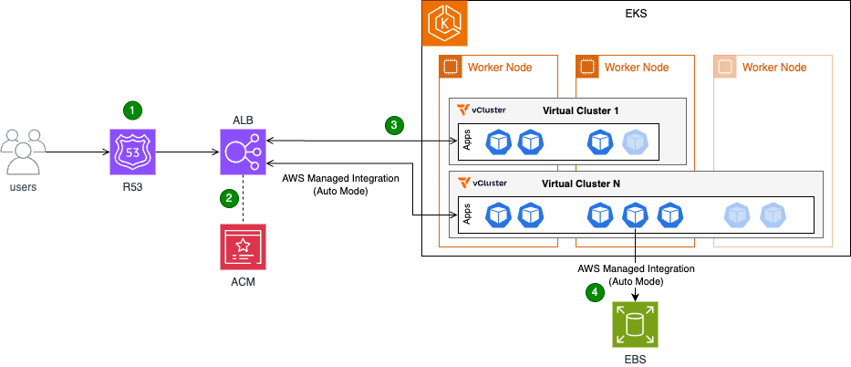
To address these challenges, Deloitte implemented a solution combining Amazon EKS with vCluster. The Amazon EKS host cluster serves as the foundation, providing the underlying compute and networking resources. On top of this infrastructure, vCluster enables the creation of lightweight, fully functional virtual clusters that act like independent Kubernetes environments. This gives QA teams dedicated spaces for their work without the overhead of managing dozens of separate Amazon EKS clusters.
Essential platform services such as Kubernetes controllers and monitoring agents are deployed once on the host cluster and shared across all virtual clusters. This approach reduces resource duplication and streamlines management. With Amazon EKS Auto Mode, the solution also brings dynamic autoscaling, ensuring that compute resources are allocated just in time to meet demand, further optimizing costs.
Users access the applications over the public internet via HTTPS requests.
Their connections are secured via HTTPS, which is terminated at the Application Load Balancer (ALB).
The Application Load Balancer (ALB) directs users to the appropriate application based on predefined rules.
Each application that users deploy runs in its own virtual cluster with dedicated Amazon Elastic Block Store (Amazon EBS) storage.
Key components:
Amazon EKS host cluster with Auto Mode enabled: The foundation of the solution, providing the underlying Kubernetes infrastructure
Virtual clusters (vCluster): Multiple isolated Kubernetes clusters running within the host cluster. Each virtual cluster represents an isolated testing environment for QA validation and application testing.
Shared controllers: These controllers run on the host cluster and are shared across all virtual clusters:
Load Balancer Controller: Manages the creation and configuration of load balancers for applications running in the virtual clusters
Storage Controller: Manages the creation of Amazon EBS volumes or Amazon Elastic File System (Amazon EFS) mount points, providing persistent storage for applications
Application Load Balancer (ALB): Fronts the host cluster nodes, distributing traffic and ensuring high availability
AWS Certificate Manager (ACM): An ACM certificate is attached to the ALB to terminate HTTPS connections and provide secure communication
Outcomes
Deloitte’s implementation of Amazon EKS with vCluster delivered measurable results. Environment provisioning time dropped from 45 minutes to under 5 minutes, representing an 89% reduction that translates to immediate productivity gains. The QA team has reclaimed around 500 hours annually, shifting focus from repetitive setup tasks to higher-value testing work. Infrastructure efficiency improved significantly through resource consolidation. By deploying workloads to a shared host cluster and enabling virtual clusters to share those resources, Deloitte saves over 50 vCPUs and more than 200 GB of memory at peak usage.
On the AWS front, consolidating to fewer Amazon EKS control planes reduced management overhead and costs. Cost optimization improved further, with up to 70% savings by running workloads on Amazon Elastic Compute Cloud (Amazon EC2) Spot Instances, with Amazon EKS Auto Mode providing efficient, automated autoscaling and provisioning. The architecture was further streamlined by implementing a single load balancer capable of serving traffic to applications across multiple virtual clusters. This reduced complexity and simplified monitoring and troubleshooting.
The vCluster itself proved transformative. Deloitte now runs more than 50 virtual clusters efficiently on a single shared Amazon EKS host cluster. Teams can now provision their own testing environments in under 5 minutes without platform team involvement, compared to submitting requests and waiting 30-45 minutes previously. Both QA and application teams now have faster access to the environments they need. Tooling complexity decreased significantly. Instead of managing more than ten separate tool deployments (reverse proxy, monitoring agents, controllers, etc.), teams now rely on a single shared stack that’s easier to maintain and operate. These improvements collectively position Deloitte with a more scalable, cost-effective, and manageable AWS environment that’s ready to grow with evolving business needs.
Walkthrough
This section provides a simplified overview of the solution, preserving the core elements implemented at Deloitte. It covers the deployment of two applications on separate virtual clusters, the ability to access the vCluster platform, and the configuration of both applications to operate under the same domain and load balancer.
Prerequisites
Before beginning the deployment, verify that the following resources are in place:
Amazon Virtual Private Cloud (Amazon VPC) and subnets: An Amazon VPC and the necessary subnets must be created
Amazon EKS Cluster: An Amazon EKS cluster should be set up within the designated Amazon VPC and subnets, with Auto Mode enabled
Service IPv4 range: The Amazon EKS service IPv4 range must be set to 10.96.0.0/12 (the service Classless Inter-Domain Routing (CIDR) range used by vCluster)
IAM roles: The following IAM roles must be created
(For Auto Mode) EKS Auto Mode Node Role with permissions for EC2, EBS, and Auto Scaling operations
Domain name: A domain name, along with the necessary certificate and DNS configuration, must be obtained
kubectl and Helm: Command-line tools for Kubernetes management
Deployment steps
The following walkthrough guides you through deploying the solution. You’ll start by creating and validating the required certificate, then deploy vCluster with Amazon EKS Auto Mode and configure the ALB. Next, you’ll access the vCluster console to create two virtual clusters. Finally, you’ll deploy an application in both virtual clusters and expose it through an Application Load Balancer using path-based routing.
The expected outcome of the preceding commands is the creation and validation of a certificate in AWS Certificate Manager (ACM) within the specified region.
Step 2: Deploy vCluster with Amazon EKS Auto Mode and Application Load Balancer
The following command configures the ingress class for ALB provisioning and the storage class for Amazon EBS persistent volumes.
The expected outcome is the successful deployment of the vCluster platform on the Amazon EKS cluster, accessible via the load balancer and domain provisioned in the previous steps.
Figure 2: vCluster environment login page.
Step 3: Access the vCluster console and create virtual clusters
Open a web browser and navigate to the vCluster domain set up earlier
Log in with the following credentials:
Username: admin
Password: password
On first login, complete the setup questions to start the 13-day vCluster platform trial by providing:
Name
Email address
Company name
Step 4: Create two virtual clusters through the console
Using the vCluster UI, create a new virtual cluster and select the “Deploy with vCluster platform (default)” option. Replace the content of the vcluster.yaml file with the following configuration:
This configuration enables synchronization between the host cluster and the virtual cluster for both ingress classes and storage classes, making host cluster resources available within the virtual cluster. It also synchronizes ingress resources from the virtual cluster back to the host cluster. The coredns section configures the virtual cluster control plane to deploy a DNS management pod, supporting DNS resolution for applications within the virtual cluster. After adding the configuration, create the cluster. After you have created the cluster and it is healthy, repeat the process to create the second cluster.
Figure 3: vCluster environment with two newly created virtual clusters.
Step 5: Deploy applications
After both clusters are up and running:
Select and connect to the virtual cluster as shown in the following figure.
Figure 4: vCluster main page and connect option to a single virtual cluster.
Download the kubeconfig file and use it to connect to the cluster.
Figure 5: Connect to virtual cluster menu.
After you have established access to the newly created virtual cluster via kubectl, run the following command to deploy the application to the cluster.
Namespace: Creates a new namespace called echoserver
Service: Creates a service named echoserver within the echoserver namespace
Deployment: Creates a deployment named echoserver in the echoserver namespace
Ingress: Creates an ingress resource that routes traffic to the echoserver service on port 80 via internet-facing load balancer (for testing purposes)
Persistent Volume Claim (PVC): Requests storage resources for the application
Note: Replace placeholders in the YAML file with the appropriate values.
Repeat the preceding steps on the second virtual cluster. Upon resource deployment, Amazon EKS adds new path-based rules to the ALB that match the deployed Ingress objects, exposing the applications.
Figure 6: Application Load Balancer rules illustrating rules from different applications through the ingress object.
Step 6: Validate the implementation
To verify that the virtual cluster setup is working correctly, perform the following validation checks:
Cluster deployment verification: Verify the successful deployment of both App1 and App2 in their respective virtual clusters. Validate pod status and service functionality
Application accessibility testing: Test that both applications are properly exposed through the single Application Load Balancer:
App1: https://<domain-name>/app1
App2: https://<domain-name>/app2
Clean up
To avoid incurring unnecessary charges, remove the deployed resources when they’re no longer needed. Start by uninstalling the vCluster Helm release, then delete the Amazon Route 53 DNS records and AWS Certificate Manager certificate:
In this post, we showed how Deloitte used Amazon EKS with vCluster to reduce environment provisioning time by 89%, reclaim 500 hours annually, and cut infrastructure costs through resource consolidation. Ready to transform your development and testing infrastructure? Start by evaluating your current environment provisioning process and identifying opportunities to consolidate workloads using Amazon EKS with vCluster. Whether you’re looking to reduce setup times from hours to minutes, empower your teams with self-service capabilities, or optimize AWS costs through resource consolidation, this solution provides a proven path forward.
Visit the Amazon EKS documentation to learn more about Auto Mode and explore how virtual clusters can help your organization achieve similar gains in speed, efficiency, and operational agility. If you have questions or feedback about this post, leave a comment in the comments section.
By the time Linus Torvalds released 7.1-rc1
and closed the 7.1 merge window, 12,996 non-merge changesets had been
pulled into the mainline repository; just over 9,000 of those arrived after the first-half summary was written. These
changes were more driver-oriented than those seen earlier, but still also
included many new features across the kernel as a whole.
Understanding what AWS Identity and Access Management (IAM) policies can control helps you build better security controls and avoid spending time on approaches that won’t work. You’ve likely encountered questions like:
Can I use AWS Organizations service control policies (SCPs) to prevent the creation of security groups that allow traffic from 0.0.0.0/0?
Can I block uploads unless objects are encrypted?
Can I prevent functions with more than 512 MB of memory allocated?
Some of these are possible with IAM policies. Others are not. The difference is determined by a fundamental principle of AWS authorization: Policies make decisions based on information available in the authorization context at the time of the API call.
In this blog post, you learn how to use the AWS Service Authorization Reference to determine what’s achievable with IAM policies, recognize scenarios that need alternative solutions, and build more effective security controls in your AWS environment.
Understanding AWS authorization context
When you make an AWS API request through the AWS Management Console, AWS Command Line Interface (AWS CLI), or AWS SDK, the specific AWS service (such as Amazon S3 or Amazon EC2) receiving the request assembles a request context containing information about that request. This context is used for policy evaluation decisions. Request context is structured using the Principal, Action, Resource, Condition (PARC) model, which has four key components.
Principal: Identifies the requester and their attributes (tags, session context)
Action: Specifies the AWS API operation being requested (for example, s3:PutObject, ec2:RunInstances)
Resource: Defines the target AWS resource using Amazon Resource Names (ARNs)
Condition: Provides additional context available at request time, such as IP address, time, encryption parameters, MFA status, and service-specific attributes
The following example shows the typical request context for an Amazon S3 object upload:
IAM policies can evaluate request metadata like encryption method and storage class being specified. However, it cannot evaluate the actual file contents, object size, or specific data patterns. Policy evaluation occurs at the time of the request, using the information present in the authorization context.
An essential resource: The Service Authorization Reference
The Service Authorization Reference is the authoritative documentation for understanding what policies can control. For every AWS service, it documents:
Actions: Every controllable operation
Resources: Resource types that can be targeted
Condition keys: The exact context information available for policy decisions
Condition keys are broadly divided into two categories. Global condition keys, which can be used across AWS services, and service-specific condition keys, which are defined for use with an individual AWS service. Use the Service Authorization Reference to find the global-condition keys or service-specific condition keys for each AWS service.
How to use the Service Authorization Reference
Follow these steps to determine if your requirement can be controlled with IAM policies:
Find the action you want: Find the API operation you want to control. Be precise, different actions have different available condition keys.
Examine available condition keys: The Condition keys column shows what context information AWS makes available for that action.
Make your feasibility determination: If the information you need isn’t listed as a condition key, you will not be able to control it with IAM policies alone.
Let’s take an example from the Amazon Elastic Compute Cloud (Amazon EC2)ec2:RunInstances action to see what you can and can’t control. In the Service Authorization Reference under the Amazon EC2 section, examine the RunInstances action and check the Resource types column. The RunInstances action affects multiple resource types, each with its own set of condition keys.
For the instance* resource type:
ec2:InstanceType: Can restrict instance types
ec2:EbsOptimized: Can require EBS optimization
aws:RequestTag/: Can enforce tagging requirements
For the network-interface* resource type:
ec2:Subnet: Can control subnet placement
ec2:Vpc: Can limit to specific virtual private clouds (VPCs)
ec2:AssociatePublicIpAddress: Can control public IP assignment
Note: These are a few examples from the many condition keys available for each resource type under the RunInstances action. The Service Authorization Reference lists dozens of condition keys across resource types (instance, network interface, security group, subnet, volume, and so on) that RunInstances affects. Consult the complete reference to see the available options for your specific use case.
Access the Service Authorization Reference programmatically
Beyond the human-readable documentation, AWS provides the Service Authorization Reference in machine-readable JSON format to streamline automation of policy management workflows. Use this programmatic access to incorporate authorization metadata into your development and security workflows. For detailed information about the JSON structure and field definitions, see the Simplified AWS service information for programmatic access. Developers can use tools like the IAM MCP Server for AWS IAM operations. This server provides AI assistants with the ability to manage IAM users, roles, policies, and permissions while following security best practices.
Using IAM policies to control specific scenarios
The following examples show how you can use IAM policies to control specific scenarios.
Example 1: Enforce AES256 server-side encryption on S3 objects
In the Amazon S3 Service Authorization Reference, under s3:PutObject action, the s3:x-amz-server-side-encryption condition key is available in the authorization context, which can be used to control the server-side encryption of S3 objects with AES-256. Here is the required policy.
Policy 1: Deny Amazon S3 object upload if the encryption doesn’t use AES-256
Policy 1 is a resource-based policy that can be applied on an S3 bucket to restrict object uploads. It denies a PutObject request when the server-side encryption isn’t using the AES-256 encryption algorithm.
Example 2: Allow different instance types based on the user’s cost center tag.
When checking the Amazon EC2 Service Authorization Reference for ec2:RunInstances, the ec2:InstanceType condition key, which is resource specific, is available. To restrict instance types based on who is launching them (rather than just what is being launched), you can either combine this with a global condition key or attach different policies to different principals. By using aws:PrincipalTag/tag-key alongside ec2:InstanceType, you can identify the user’s cost center from their IAM identity tags and then apply different instance type restrictions accordingly. This allows a single policy to dynamically enforce different permissions based on the requester’s identity.
Policy 2: Restricting EC2 instance types by cost center
This is an identity-based policy that you can attach to IAM users, groups, or roles to control EC2 instance launches based on cost allocation. In the first statement, aws:PrincipalTag, which is a global condition key (tags attached to the IAM user or role), is used to determine which instance types are allowed. Users tagged with CostCenter=Development can only launch cost-effective T3 instance types (t3.micro, t3.small, t3.medium, and so on)with the service specific key ec2:InstanceType.
In the second statement, users tagged with CostCenter=Production can launch more powerful instance types from the M5 (general purpose), C5 (compute optimized), and R5 (memory optimized) families. This approach lets organizations enforce cost controls and allocate resources based on workload requirements. Each cost center maintains flexibility for its specific needs.
Note: Additional resources are required in the IAM policy to successfully launch EC2 instances. For the complete list, see Launch Instances.
Example 3: Users can only access and update DynamoDB items where the partition key matches their username.
You have identified that GetItem, PutItem,and UpdateItem actions are required. Corresponding to these actions, you can use the condition key to expose partition key values in the authorization context as described in the Amazon DynamoDB Service Authorization Reference
The policy allows users to perform read and write actions (GetItem, PutItem, and UpdateItem) on the UserProfiles table, but only for items where the partition key value equals their own username (using the ${aws:username} policy variable). For example, if user alice attempts to access an item with partition key bob, the request will be denied.
Scenarios that need more than policies alone
Some requirements can’t be met using IAM policies. Here are three common scenarios that aren’t achievable with IAM policies alone.
Scenario 1: Block users from creating security group rules that allow traffic from 0.0.0.0/0 on TCP port 22
Upon checking the Amazon EC2 Service Authorization Reference, you will find that the ec2:AuthorizeSecurityGroupIngress action is required in an IAM policy to add an inbound access rules to a security group.
To verify this in the Service Authorization Reference, navigate to the Amazon EC2 Service Authorization Reference and search for the AuthorizeSecurityGroupIngress action, which is the action that creates security group rules. After you locate this action, review the Condition keys column and look for condition keys related to CIDR blocks, IP ranges, ports, or protocols. Available condition keys for ec2:AuthorizeSecurityGroupIngress include:
Notice there are no condition keys for CIDR blocks (such as 0.0.0.0/0), port numbers (such as 22), or protocols (such as TCP). The authorization context doesn’t include information about the specific CIDR blocks, ports, or protocols being added to the security group rule, so IAM policies can’t control these attributes.
Scenario 2: Prevent creation of Lambda functions with more than 512 MB of memory allocated
Following the same verification methodology described in Scenario 1, navigate to the AWS Lambda Service Authorization Reference and examine the CreateFunction action’s condition keys for the function* resource type.
Available condition keys for lambda:CreateFunction with the function* resource type include:
lambda:CodeSigningConfigArn: Filters access by the ARN of the code signing
configuration-lambda:Layer: Filters access by the ARN of a version of an AWS Lambda layer
lambda:VpcIds: Filters access by the ID of the VPC configured for the Lambda function
There is no condition key for memory allocation (MemorySize parameter), timeout settings, storage configuration (EphemeralStorage), or runtime selection. Because memory allocation isn’t exposed in the authorization context, IAM policies can’t restrict this parameter.
Keep these principles in mind when working with IAM policies:
Policies control what’s in the authorization context, not all elements you see in API documentation
The Service Authorization Reference is authoritative; if something isn’t listed as a condition key, you can’t control it with policies
Different actions have different available contexts even within the same service
Alternative approaches exist. AWS Config, EventBridge, and service-specific controls can be used to achieve your goals when policies alone can’t
Layered security is essential; combine preventive, detective, and responsive controls to help ensure that your data is secure
Conclusion
In this post, you learned how to use the AWS Service Authorization Reference to determine what’s achievable with IAM policies and recognize scenarios that require alternative solutions. By understanding that policies can only make decisions based on information available in the authorization context, you can build more effective security controls and avoid spending time on approaches that won’t work.
The Service Authorization Reference is your authoritative source for understanding policy capabilities. When you need to implement a control, start there to see if the required condition keys exist. If they don’t, you will need to layer in detective or responsive controls using services like AWS Config, Amazon EventBridge, or AWS Lambda.
Remember that effective AWS security isn’t about finding one perfect control, it’s about combining preventive, detective, and responsive measures to create defense in depth. IAM policies are powerful tools for prevention and work as part of a comprehensive security strategy.
Greg Kroah-Hartman has announced the release of the 7.0.2, 6.18.25, 6.12.84, and 6.6.136 stable kernels. As usual, each
contains important fixes throughout; users are advised to upgrade.
NAB Show 2026 wrapped up last week in Las Vegas, and we left with something special in hand: the NAB Show Product of the Year Award in the Cloud Computing and Storage category—this time for Backblaze B2 Neo.
It’s a meaningful recognition, and one that reflects where we see the media and AI infrastructure market heading. Here’s a look at what the recognition means, and why B2 Neo matters.
What this recognition means
Winning the NAB Product of the Year Award reflects something we genuinely believe: that storage infrastructure is a foundational capability for modern media and AI platforms, not an afterthought or a separate vendor relationship to manage.
The NAB Show brings together the best of the media and entertainment industry, and having B2 Neo recognized in this context—among platforms solving real, production-scale problems across streaming, OTT, AI-driven media processing, and large-scale content delivery—is meaningful validation that the approach resonates.
B2 Neo launched in February 2026 and is already supporting production workloads including AI training pipelines, high-performance computing environments, and large-scale media delivery. The response from platform providers has reinforced what we know: organizations want to offer integrated, high-performance storage without building it from scratch, and they want the economics to make sense.
What is B2 Neo?
B2 Neo is a high-performance, S3-compatible cloud object storage solution purpose-built for platforms running data-intensive media and AI workloads. But describing it simply as “cloud storage” undersells the point.
The key distinction: B2 Neo is a white-label service. Rather than selling storage directly to end users, B2 Neo enables platform providers—like media workflow vendors—to offer fully integrated storage under their own brand. Partners launch their own storage service with custom endpoints, pricing, and user experiences, without having to build or operate the underlying infrastructure themselves.
The result is that platforms can go from “we don’t offer storage” to “we have a native, high-performance storage tier” in weeks rather than years, with none of the capital investment or engineering overhead that building it in-house would require.
Why it was built
The problem B2 Neo addresses has been growing for years, but it’s become acute as streaming, OTT, and AI-driven media workflows scale up.
Compute has gotten fast, distributed, and relatively affordable. GPU clusters, edge networks, and CDNs can all handle increasingly complex workloads. But storage has often lagged behind—fragmented across providers, expensive to move data in and out of, and either too costly or too operationally burdensome to build in-house.
The consequence is real: GPU clusters sit idle waiting on data. Streaming pipelines bottleneck on access speeds. Media organizations duplicate content across storage systems because no single layer integrates cleanly into the rest of the stack.
B2 Neo was designed to remove that bottleneck. It delivers up to 1Tbps of throughput to ensure that compute resources—GPU clusters, streaming systems, edge delivery networks—are never waiting on storage. It combines that performance with Backblaze’s 17+ years of operational experience at exabyte scale, and wraps it in an API-first architecture that plugs directly into partner platforms.
How it works
From a technical standpoint, B2 Neo delivers high aggregate throughput using cost-efficient, disk-based infrastructure with strategically deployed flash layers—a write-through cache design that captures the performance benefits of flash without the cost and scalability limitations that come with an all-flash architecture at the multi-petabyte scale that media and AI workloads require.
For workloads where throughput matters as much as latency—moving large video files, training AI models, serving content at scale—this approach is particularly effective. It allows platforms to maintain a centralized data repository and efficiently deliver data to compute providers, edge networks, and CDNs without duplicating data across storage systems.
API-driven provisioning lets partners programmatically create and manage storage accounts, permissions, and billing within their existing systems. Whether a partner is running an OTT platform, a media asset management system, or an AI training pipeline, B2 Neo integrates as a native extension of that environment rather than an external dependency to work around.
Included egress and free API calls round out the picture, eliminating the usage-based fees that typically make storage decisions financially complicated.
What’s next
This is a product that will keep evolving alongside the media and AI infrastructure landscape. We’re working closely with early partners to expand B2 Neo’s capabilities—performance, integration depth, provisioning flexibility—and we’ll have more to share as those conversations develop.
If you’re building or operating a platform that would benefit from embedded, high-performance storage, we’d love to talk. Reach out to our team to learn more about what a B2 Neo partnership looks like.
Late March took me to Seattle for the Specialist Tech Conference, one of the most energizing gatherings of AWS specialists from around the world. It was an incredible opportunity to connect with peers, exchange experiences, and go deep on the latest advancements in Generative AI and Amazon Bedrock — and a powerful reminder of something I truly believe in: when specialists come together to challenge each other, explore edge cases, and co-create solutions, the impact goes far beyond the meeting room. In a fast-moving space like AI, having a strong internal community isn’t a nice-to-have — it’s a competitive advantage.
Now, let’s get into this week’s AWS news…
Headlines
Anthropic partnership: Claude on AWS Trainium and Graviton, and Claude Cowork in Amazon Bedrock – This week, AWS and Anthropic deepened their product collaboration in meaningful ways for builders. Anthropic is now training its most advanced foundation models on AWS Trainium and Graviton infrastructure, co-engineering directly at the silicon level with Annapurna Labs to maximize computational efficiency from the hardware up through the full stack.
Claude Cowork is now available in Amazon Bedrock — Claude Cowork brings Anthropic’s collaborative AI capabilities directly to enterprise builders within the AWS ecosystem, enabling teams to work alongside Claude as a true collaborator, not just a tool. You can now deploy Claude Cowork within your existing Amazon Bedrock environment, keeping your data secure within AWS while leveraging the full power of Claude for team-based AI workflows.
Claude Platform on AWS (Coming soon) — A unified developer experience to build, deploy, and scale Claude-powered applications without leaving AWS. If you’re building with Generative AI on AWS, this is a significant step forward in what you’ll be able to do with Claude directly through Amazon Bedrock.
Meta signs agreement with AWS to power agentic AI on Amazon’s Graviton chips — Meta has signed an agreement to deploy AWS Graviton processors at scale, starting with tens of millions of Graviton cores to power CPU-intensive agentic AI workloads — including real-time reasoning, code generation, search, and multi-step task orchestration.
Last week’s launches
Here are some launches and updates from this past week that caught my attention:
AWS Lambda functions can now mount Amazon S3 buckets as file systems with S3 Files — You can now mount Amazon S3 buckets as file systems in AWS Lambda using S3 Files, enabling your functions to perform standard file operations without downloading data for processing. Built on Amazon EFS, S3 Files provides the simplicity of a file system with the scalability, durability, and cost-effectiveness of S3 — and multiple Lambda functions can connect to the same file system simultaneously, sharing data through a common workspace. This is particularly valuable for AI and machine learning workloads where agents need to persist memory and share state across pipeline steps.
Amazon EKS Hybrid Nodes gateway for hybrid Kubernetes networking — Amazon Elastic Kubernetes Service now offers the Amazon EKS Hybrid Nodes gateway, which automates networking between your EKS cluster VPC and Kubernetes Pods running on EKS Hybrid Nodes. You can now eliminate the need to make on-premises pod networks routable or coordinate network infrastructure changes, greatly simplifying hybrid Kubernetes environments. The gateway automatically enables pod-to-pod traffic across cloud and on-premises environments, control plane-to-webhook communication, and connectivity for AWS services like Application Load Balancers, and is available at no additional charge.
Amazon Aurora Serverless: Up to 30% better performance, smarter scaling, and still scales to zero — Amazon Aurora Serverless just got faster and smarter, with up to 30% better performance than the previous version and an enhanced scaling algorithm designed to handle workloads where multiple tasks compete for resources — like busy APIs and agentic AI applications with bursts of activity and long idle windows. You can now run even more demanding workloads serverlessly, paying only for what you use, and automatically scaling to zero when not in use. All improvements are available in platform version 4 at no additional cost.
Amazon Bedrock AgentCore adds new features to help developers build agents faster — Amazon Bedrock AgentCore introduces a managed harness (preview), the AgentCore CLI, and AgentCore skills for coding assistants, helping developers go from idea to working agent prototype faster. The managed harness lets you define an agent by specifying a model, system prompt, and tools and run it immediately with no orchestration code required — and when you’re ready for full control, you can export the harness orchestration as Strands-based code. The AgentCore CLI deploys your agents with the governance and auditability of infrastructure-as-code (AWS CDK today, Terraform coming soon), and is available in 14 AWS Regions at no additional charge.
For a full list of AWS announcements, be sure to keep an eye on the What’s New with AWS page.
Other AWS news
Here are some additional posts and resources that you might find interesting:
Introducing granular cost attribution for Amazon Bedrock — This post walks through how Amazon Bedrock’s granular cost attribution works and covers practical example cost tracking scenarios. You can now tag and track Bedrock usage costs at a finer level of detail — useful for organizations running multiple teams or projects on Bedrock who need precise cost visibility and chargeback capabilities.
Automating Incident Investigation with AWS DevOps Agent and Salesforce MCP Server — This post (co-written with Salesforce) shows how AWS DevOps Agent, integrated with the Salesforce MCP Server, automates the full lifecycle of infrastructure incident investigation — from identifying issues and diagnosing root causes to notifying customers through Salesforce Service Cloud. It’s a compelling real-world example of how AI agents and MCP-based tool connectivity are reshaping DevOps workflows in production, dramatically reducing mean time to resolution.
Microcredentials from AWS are now free — Here’s why that matters — You can now access AWS microcredentials at no cost through AWS Skill Builder in all countries where the platform is offered. Unlike traditional multiple-choice certifications, microcredentials are hands-on assessments that place builders in simulated business scenarios where they configure, troubleshoot, and optimize directly in a live AWS environment — the same way they would on the job. A great opportunity to validate real cloud skills without a cost barrier.
Amazon SageMaker AI now supports optimized generative AI inference recommendations — You can now use Amazon SageMaker AI to automatically identify optimized deployment configurations for your generative AI models, including instance type, container, and inference parameters. This new capability takes the guesswork out of tuning inference infrastructure, helping you reduce costs and improve latency for your AI applications in production.
Upcoming AWS events
Check your calendar and sign up for upcoming AWS events:
What’s Next with AWS — Tune in on April 28 for What’s Next with AWS, a virtual event featuring the latest announcements and product updates directly from AWS teams. A great opportunity to get up to speed on what’s new before diving into the week’s launches.
AWS Summits — AWS Summits are free in-person events where you can explore the latest in cloud and AI innovation, learn best practices, and network with builders and experts. Coming up in May: Singapore (May 6), Tel Aviv (May 6), Warsaw (May 6), Stockholm (May 7), Sydney (May 13–14), Hamburg (May 20), Seoul (May 20), Amsterdam (May 27), Bangkok (May 28), Milan (May 28), and Mumbai (May 28). And in June, join us in Los Angeles (June 10). Check the full schedule and register at the link above.
AWS Community Days — Community-led conferences where content is planned, sourced, and delivered by community leaders, featuring technical discussions, workshops, and hands-on labs. Upcoming events include Athens, Greece (April 28), Vancouver, Canada (May 1), İstanbul, Türkiye (May 9), and Panama City, Panama (May 23). If you’re in Latin America, mark your calendar for the AWS Community Day Belo Horizonte (August 22) — registration is open at awscommunityday.com.br.
Join the AWS Builder Center to connect with builders, share solutions, and access content that supports your development. Browse here for upcoming AWS-led in-person and virtual events and developer-focused events.
That’s all for this week. Check back next Monday for another Weekly Roundup!
— Daniel Abib
This post is part of our Weekly Roundup series. Check back each week for a quick roundup of interesting news and announcements from AWS!
The collective thoughts of the interwebz
Manage Consent
To provide the best experiences, we use technologies like cookies to store and/or access device information. Consenting to these technologies will allow us to process data such as browsing behavior or unique IDs on this site. Not consenting or withdrawing consent, may adversely affect certain features and functions.
Functional
Always active
The technical storage or access is strictly necessary for the legitimate purpose of enabling the use of a specific service explicitly requested by the subscriber or user, or for the sole purpose of carrying out the transmission of a communication over an electronic communications network.
Preferences
The technical storage or access is necessary for the legitimate purpose of storing preferences that are not requested by the subscriber or user.
Statistics
The technical storage or access that is used exclusively for statistical purposes.The technical storage or access that is used exclusively for anonymous statistical purposes. Without a subpoena, voluntary compliance on the part of your Internet Service Provider, or additional records from a third party, information stored or retrieved for this purpose alone cannot usually be used to identify you.
Marketing
The technical storage or access is required to create user profiles to send advertising, or to track the user on a website or across several websites for similar marketing purposes.

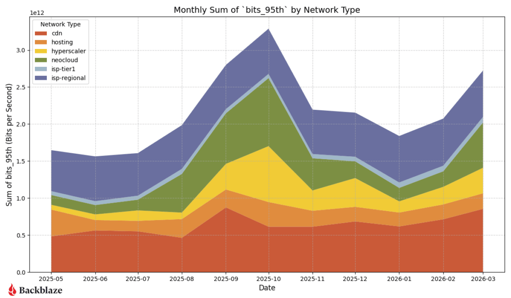
 ISP-Regional traffic continues to be a hotspot on the heatmap, as expected. This region has the largest footprint behind it and connections to internet exchanges (IX). This quarter, with a lull in neocloud and hyperscaler traffic over the winter period, we saw an increase in traffic to our CDN partners. The amount of traffic to CDN networks in the US-West, US-East, and EU-Central regions all increased quarter over quarter.

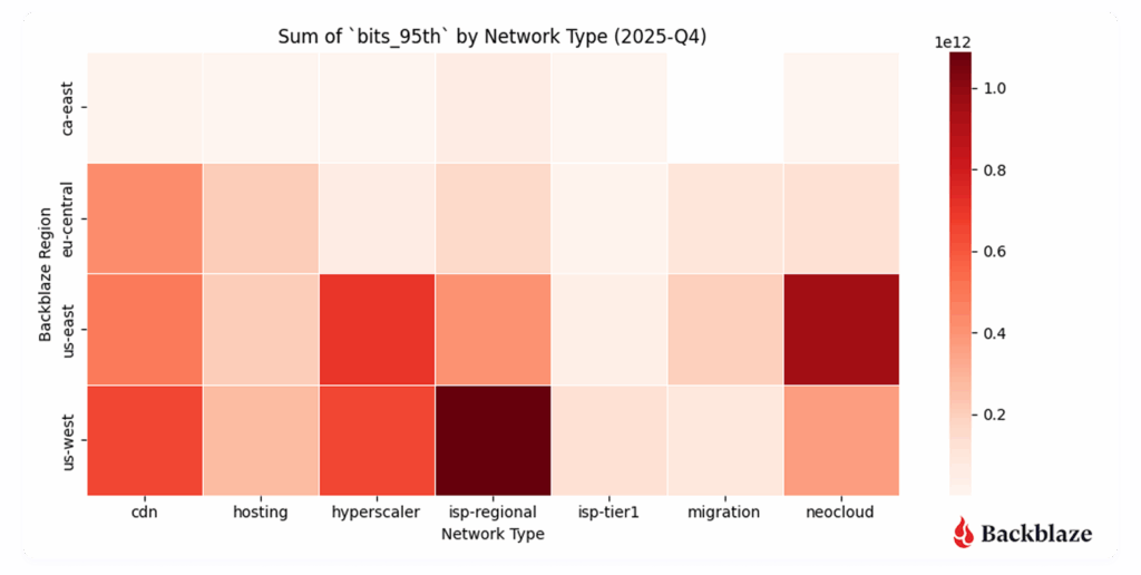
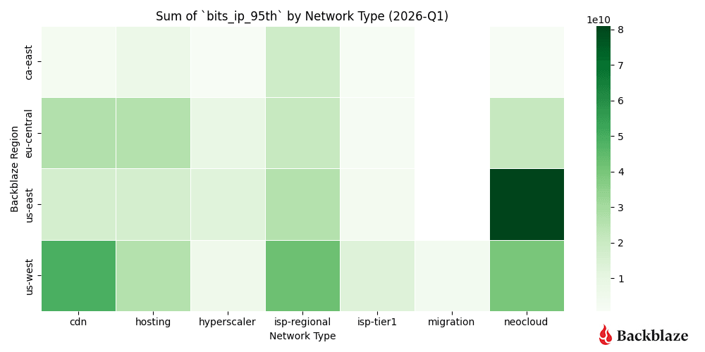
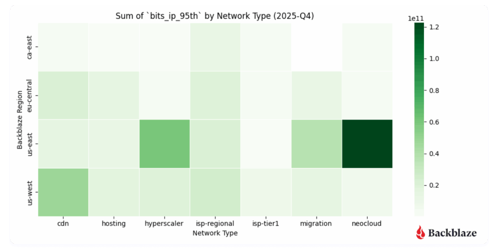

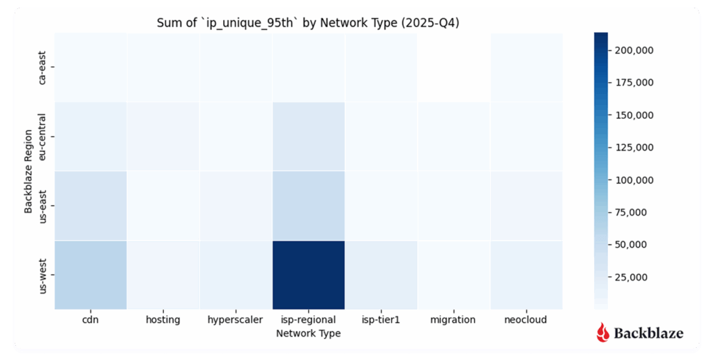
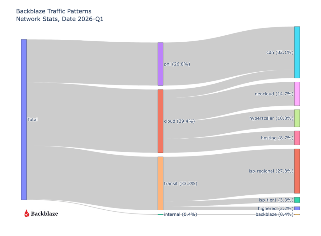

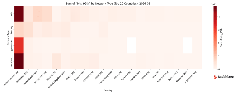
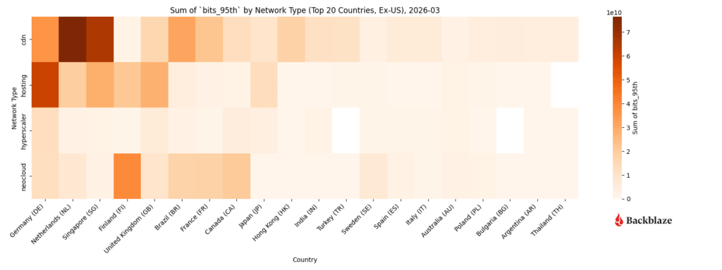
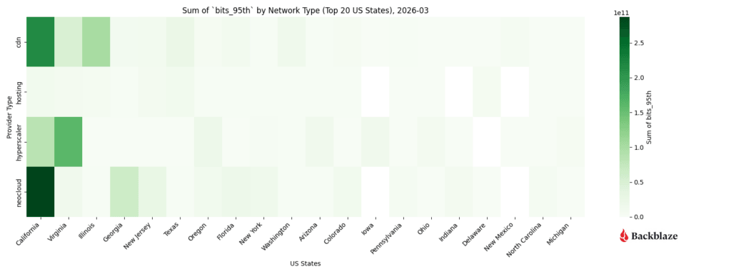

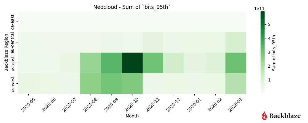
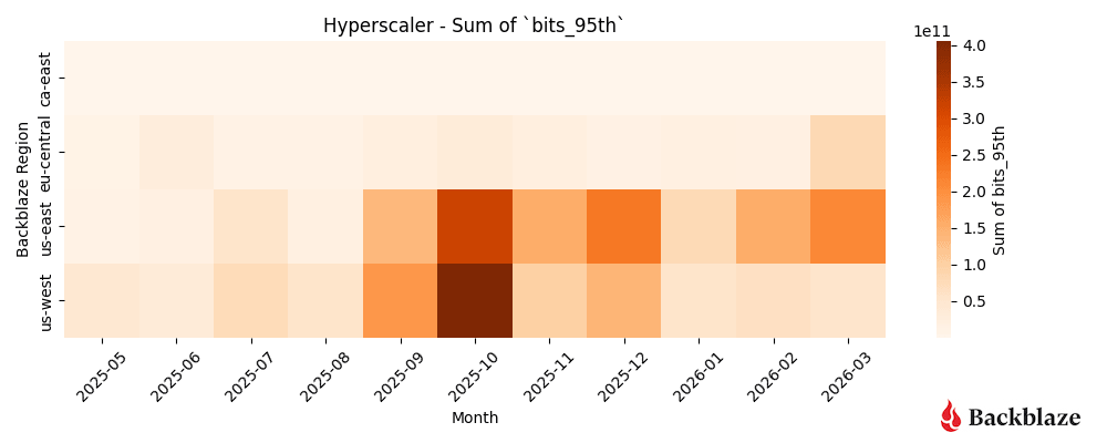

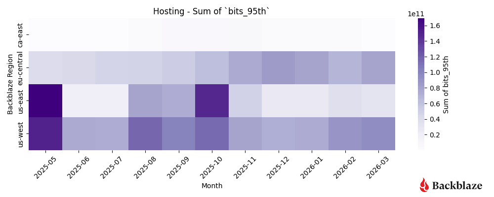
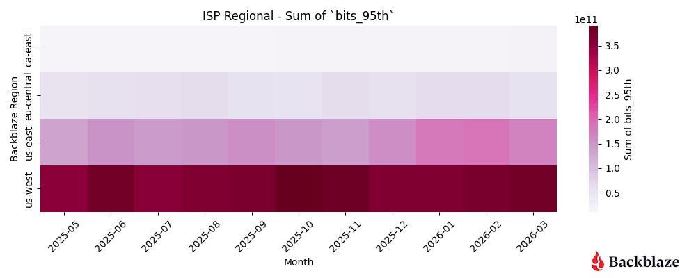

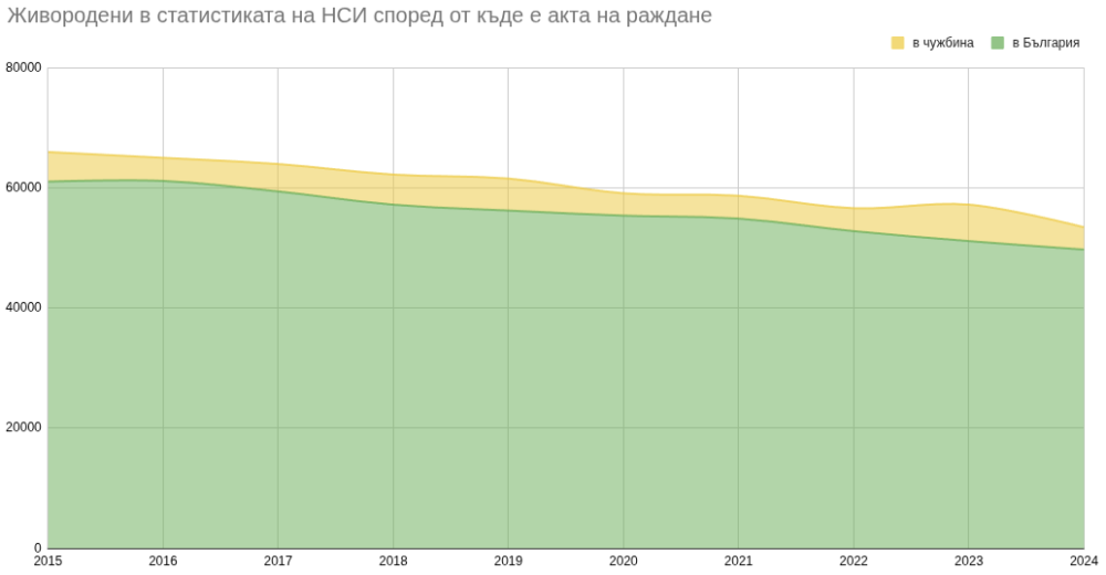
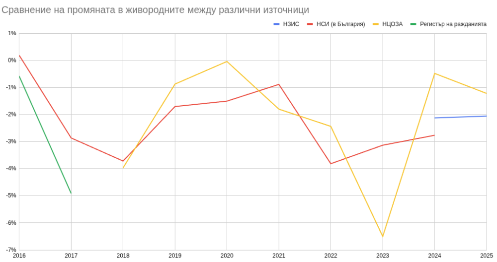
 Yes
 No