Tag Archives: Advanced (300)

AWS Glue crawlers support cross-account crawling to support data mesh architecture

2023-03-27 Sandeep Adwankar

Post Syndicated from Sandeep Adwankar original https://aws.amazon.com/blogs/big-data/aws-glue-crawlers-support-cross-account-crawling-to-support-data-mesh-architecture/

Data lakes have come a long way, and there’s been tremendous innovation in this space. Today’s modern data lakes are cloud native, work with multiple data types, and make this data easily available to diverse stakeholders across the business. As time has gone by, data lakes have grown significantly and have evolved to data meshes as a way to scale. Thoughtworks defines a data mesh as “a shift in a modern distributed architecture that applies platform thinking to create self-serve data infrastructure, treating data as the product.”

Data mesh advocates for decentralized ownership and delivery of enterprise data management systems that benefit several personas. Data producers can use the data mesh platform to create datasets and share them across business teams to ensure data availability, reliability, and interoperability across functions and data subject areas. Data consumers now have better data sharing with data mesh and federation across business units without compromising data security. The data governance team can support distributed data, where all data is accessible to those with the proper authority to access it. With data mesh, data doesn’t have to be consolidated into a single data lake or account and can remain within different databases and data lakes. An essential capability needed in such a data lake architecture is the ability to continuously understand changes in the data lakes in various other domains and make those available to data consumers. Without such a capability, manual work is needed to understand producers’ updates and make them available to consumers and governance.

AWS customers use a modern data architecture to facilitate governance and data sharing across logical or physical governance boundaries to create data domains aligned to lines of business. Each line of business creates and manages their dataset on Amazon Simple Storage Service (Amazon S3) and uses AWS Glue crawlers to discover new datasets and register them to the AWS Glue Data Catalog, add new tables and partitions, and detect schema changes. These datasets are shared with data consumers that access the data using services like Amazon Athena, Amazon Redshift, Amazon EMR, and more.

In the post Introducing AWS Glue crawlers using AWS Lake Formation permission management, we introduced a new set of capabilities in AWS Glue crawlers and AWS Lake Formation that simplifies crawler setup and supports centralized permissions for in-account and cross-account crawling of S3 data lakes. In this post, we demonstrate the same capability for a data mesh architecture in which we establish a central governance layer to catalog the data owned by the data producer and share it with the data consumer for ease of discovery. The AWS Glue crawler cross-account capability allows you to crawl data sources in different producer accounts while still having those changes cataloged in a centralized governance account. Customers prefer the central governance experience over writing bucket policies separately in each bucket owning the account of a data mesh producer. To build a data mesh architecture, now you can author permissions in a single Lake Formation governance to manage access to data locations and crawlers spanning multiple accounts in the data mesh.

According to the Allstate Corporation:

“By leveraging the power of AWS Lake Formation in our modern data architecture, we will be able to further unlock the potential of our data and empower our analytics community to drive innovation and build data-driven applications. The granular data access and collaboration provided by this architecture will enable us to build a truly unified data and analytics experience, bringing us one step closer to realizing our vision of becoming a fully data-driven enterprise.”

– Prashant Mehrotra, Director – Machine Learning and R&D, Allstate

In this post, we walk through the creation of a simplified data mesh architecture that shows how to use an AWS Glue crawler with Lake Formation to automate bringing changes from data producer domains to data consumers while maintaining centralized governance.

Solution overview

In a data mesh architecture, you have several producer accounts that own S3 buckets, several consumer accounts who wants to access shared datasets, and a central governance account to manage data shares between producers and consumers. This central governance account doesn’t own any S3 bucket or actual tables.

The following figure shows a simplified data mesh architecture with a single producer account, a centralized governance account, and a single consumer account. The data mesh producer account hosts the encrypted S3 bucket, which is shared with the central governance account. The central governance account registers the S3 bucket with Lake Formation using an AWS Identity and Access Management (IAM) role, which has permissions to the S3 bucket and AWS Key Management Service (AWS KMS). The central account creates the database for storing the dataset schema and shares it with the producer account. The producer account, as the S3 bucket owner, runs a crawler to crawl the buckets registered with the central account using Lake Formation permissions and populates the database. Now the shared database with new datasets are available to share with consumers in the data mesh. The central governance account can now share the database with a consumer admin, who can delegate access to other personas (such as data analysts) in the consumer account for data access.

shows a simplified data mesh architecture with a single producer account, a centralized governance account, and a single consumer account

In the following sections, we provide AWS CloudFormation templates to set up the resources in each account. Then we provide the steps to configure the crawler, manage permissions and sharing, and validate the solution by running queries with Athena.

Prerequisites

Complete the following steps in each account (producer, central governance, and consumer) to update the Data Catalog settings to use Lake Formation permissions to control catalog resources instead of IAM-based access control:

Sign in to the Lake Formation console as admin.
If this is the first time accessing the Lake Formation console, add yourself as the data lake administrator.
In the navigation pane, under Data catalog, choose Settings.
Uncheck Use only IAM access control for new databases.
Uncheck Use only IAM access control for new tables in new databases.
Keep Version 3 as the current cross-account version.
Choose Save.

Set up resources in the central governance account

The CloudFormation template for the central account creates a CentralDataMeshOwner user assigned as Lake Formation admin. The CentralDataMeshOwner user in the central governance account performs the necessary steps to share the central catalogs with the producer and consumer accounts. The CentralDataMeshOwner user also sets up a custom Lake Formation service role to register the S3 data lake location. Complete the following steps:

Log in to the central governance account console as IAM administrator.
Choose Launch Stack to deploy the CloudFormation template:
For DataMeshOwnerUserName, keep the default (CentralDataMeshOwner).
For ProducerAWSAccount, enter the producer account ID.
Create the stack.
After the stack launches, on the AWS CloudFormation console, navigate to the Resources tab of the stack.
Note down the value of RegisterLocationServiceRole.
Choose the LFUsersPassword value to navigate to the AWS Secrets Manager console.
In the Secret value section, choose Retrieve secret value.
Note down the secret value for the password for IAM user CentralDataMeshOwner.

Set up resources in the producer account

The CloudFormation template for the producer account creates the following resources:

IAM user LOBProducerSteward
S3 bucket retail-datalake-<producer account id >-<producer region>
KMS key used for bucket encryption
Required S3 bucket policies to provide access to the central governance account
AWS Glue crawler and crawler IAM role with necessary permissions

Complete the following steps:

Log in to the producer account console as IAM administrator.
Choose Launch Stack to deploy the CloudFormation template:
For CentralAccountID, enter the central account ID.
For CentralAccountLFServiceRole, enter the value of RegisterLocationServiceRole from CloudFormation noted earlier.
Create the stack.
When the stack is complete, on the AWS CloudFormation console, navigate to the Resources tab of the stack.
Note down the AWSGlueServiceRole value.
Choose the ProducerStewardUserCredentials value to navigate to the Secrets Manager console.
In the Secret value section, choose Retrieve secret value.
Note down the secret value for the password for IAM user LOBProducerSteward.
On the Amazon S3 console, check the bucket policies for retail-datalake-<producer account id >-<producer region> and make sure it is shared with the central governance account IAM role.

This is required for registering the bucket with Lake Formation in the central account so that the account can manage the data sharing.

On the AWS KMS console, check that the bucket is encrypted with the customer managed key and the key is shared with the central governance account.

Set up resources in the consumer account

The CloudFormation template for the consumer account creates the following resources:

IAM user ConsumerAdminUser assigned to the data lake admin
IAM user LFBusinessAnalyst1
S3 bucket for Athena output
Athena workgroup

Complete the following steps:

Log in to the consumer account console as IAM administrator.
Choose Launch Stack to deploy the CloudFormation template:
Create the stack.
When the stack is complete, on the AWS CloudFormation console, navigate to the Resources tab of the stack.
Choose the AllConsumerUsersCredentials value to navigate to the Secrets Manager console.
In the Secret value section, choose Retrieve secret value.
Note down the secret value for the password for the IAM user ConsumerAdminUser.

Now that all the accounts have been set up, we set up cross-account sharing on AWS with a central governance account to manage sharing of permissions across producers and consumers.

Configure the central governance account to manage sharing with the producer account

Sign in to the central governance account as CentralDataMeshOwner using the password noted earlier through the central governance account CloudFormation stack. Then complete the following steps:

On Lake Formation console, choose Data lake locations under Register and ingest in the navigation pane.
For Amazon S3 path, provide the path retail-datalake-<producer account id >-<region>.
For IAM role, choose the IAM role created using the CloudFormation stack.

This role has permissions for the accessing the encrypted S3 bucket and its key. Do not choose the role AWSServiceRoleForLakeFormationDataAccess.

Choose Register location.
In the navigation pane, choose Databases.
Choose Create database.
For Database name¸ enter datameshtestdatabase.
Choose Create database.
In the navigation pane, choose Data locations and choose Grant.
Select External account and provide the producer account for AWS account ID, AWS organization ID, or IAM principal ARN.
For Storage location, provide the data lake bucket path.
Select Grantable, then choose Grant.
Choose Data lake permissions, then choose Grant.
Select External accounts and provide the producer account number.
For Databases, choose datameshtestdatabase.
For Database permissions and Grantable permissions, select Create table, Alter, and Describe.
Choose Grant.

Configure the crawler in the producer account to populate the schema

Sign in to producer account as LOBProducerSteward with the password noted earlier through the producer account CloudFormation stack, then complete the following steps:

On the AWS RAM console, accept the pending resource share from the central account.
On the Lake Formation console, choose Databases under Data catalog in the navigation pane.
Choose datameshtestdatabase, and on the Action menu, choose Create resource link.
For Resource link name, enter datameshtestdatabaselink.
Choose Create.
On the AWS Glue console, choose Crawlers in the navigation pane.
Choose the crawler CrossAccountCrawler-<accountid>.
Choose Edit, then choose Configure security settings.
Select Use Lake Formation credentials for crawling S3 data source.
Select In a different account and provide the account ID of the central governance account.
Choose Next.
Choose datameshtestdatabaselink as the database and choose Update.
In the navigation pane, choose Data locations and choose Grant.
Select My account, and choose the crawler IAM role for IAM users and roles.
For Storage locations, choose the bucket retail-datalake-<accountid>-<region>.
For Registered account location, enter the central account ID.
Choose Grant.
Alternatively, you can also use the AWS CLI to grant data location permission on bucket registered in central account to the crawler role using below command:
```
aws lakeformation grant-permissions 
--principal DataLakePrincipalIdentifier="<Crawler Role ARN>" 
--permissions "DATA_LOCATION_ACCESS” 
--resource ‘{ "DataLocation": {"ResourceArn":"<S3 bucket arn>", "CatalogId": "<Central Account id>"}}'
```
For using CLI, refer to Installing or updating the latest version of the AWS CLI.
In the navigation pane, choose Data lake permissions.
Choose the crawler IAM role for the principal account.
Choose datameshtestdatabase for the database.
For Database permissions, select Create, Describe, and Alter.
Choose Grant.
Choose the crawler IAM role for the principal account.
Choose datameshtestdatabaselink for the database.
For Resource link permissions, select Describe.
Choose Grant.
Run the crawler.

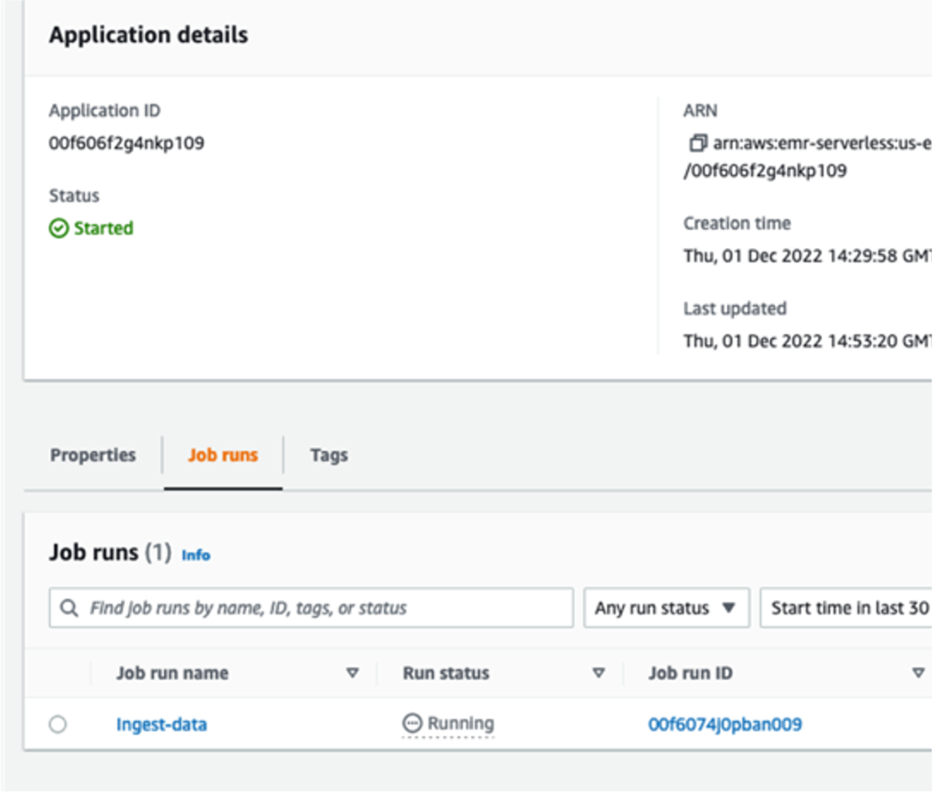
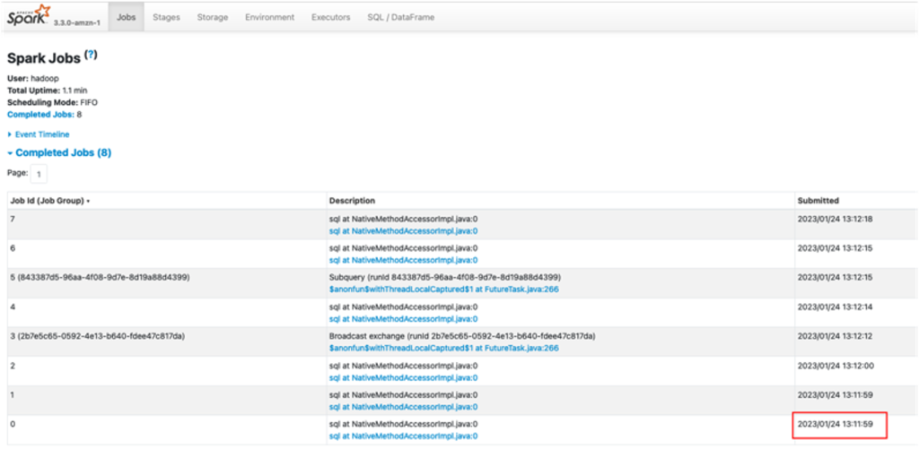
The following screenshot shows the details after a successful run.

When the crawler is complete, you can validate the table created under the database datameshtestdatabaselink.

This table is owned by the producer account and available in the central governance account under the shared database datameshtestdatabase. Now the data lake admin in the central governance account can share the database and populated table with the consumer account.

Configure the central governance account to manage sharing of read-only access with the consumer account

Sign in to the central governance account as CentralDataMeshOwner with the password noted earlier through the central governance account CloudFormation stack, then complete the following steps:

Grant database permissions to the consumer account.
For Principals, choose external account and provide <consumer accountID>
For Databases, select datameshtestdatabase.
For Database permissions, select Describe.
For Grantable permissions¸ select Describe.
Choose Grant.
Grant table permissions to the consumer account.
For Principals, choose external account and provide <consumer accountID>.
For Databases, select datameshtestdatabase.
For Tables, select retail_datalake_<accountID>_<region>.
For Table permissions, select Select and Describe.
For Grantable permissions¸ select Select and Describe.
Choose Grant.

Configure the consumer account as the consumer account data lake admin

Sign to the consumer account as ConsumerAdminUser with the password noted earlier through the consumer account CloudFormation stack. (Note that in the consumer account Lake Formation configuration, both ConsumerAdminUser and LFBusinessAnalyst1 have the same password.)

On the AWS RAM console, accept the resource share from the central account.
On the Lake Formation console, validate that the shared database datameshtestdatabase is available and create the resource link datameshtestdatabaselink using the shared database.

The following screenshot shows the details after the resource link is created.

On the Lake Formation console, choose Grant.
Choose LFBusinessAnalyst1 for IAM users and roles.
Choose datameshtestdatabase for the database under Named data catalog resources.
Select Describe for Database permissions.
On the Lake Formation console, choose Grant.
Choose LFBusinessAnalyst1 for IAM users and roles.
Choose datameshtestdatabaselink for the database under Named data catalog resources.
Select Describe for Resource link permissions.
On the Lake Formation console, choose Grant.
Choose LFBusinessAnalyst1 for IAM users and roles.
Choose retail_datalake_<accountid>_<region> for the table under Named data catalog resources.
Select Select and Describe for Table permissions.

Run queries in the consumer account

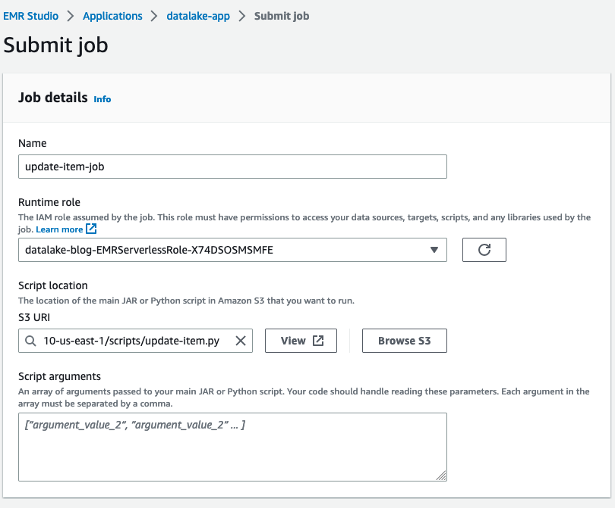
Sign to the consumer account console as LFBusinessAnalyst1 with the password noted earlier through the consumer account CloudFormation stack, then complete the following steps:

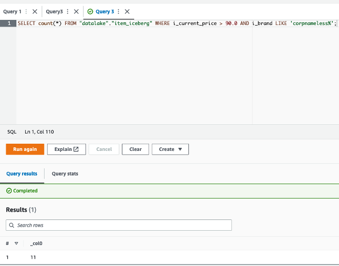
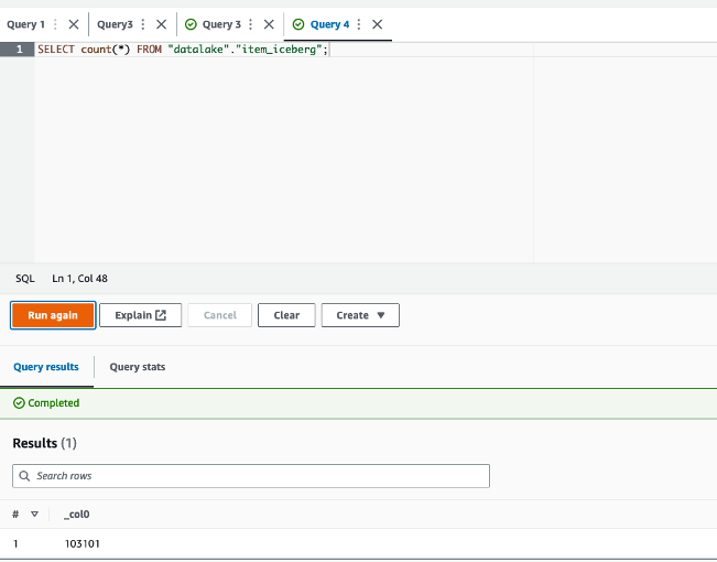
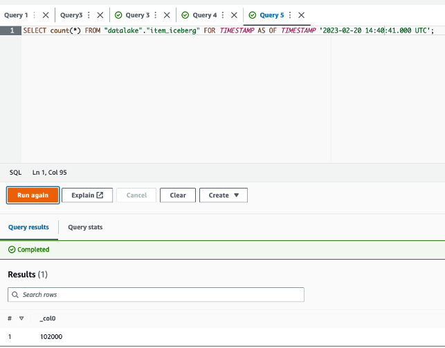
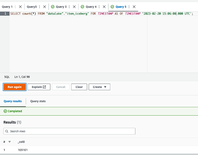
On the Athena console, and choose lfconsumer-workgroup as the Athena workgroup.
Run the following query to validate access:

select * from datameshtestdatabaselink.retail_datalake_<accountid>_<region>

We have successfully registered the dataset and created a Data Catalog in the central governance account. We crawled the data lake that was registered with the central governance account using Lake Formation permissions from the producer account and populated the schema. We granted Lake Formation permission on the database and table from the central account to the consumer user and validated consumer user access to the data using Athena.

Clean up

To avoid unwanted charges to your AWS account, delete the AWS resources:

Sign in to the CloudFormation console as the IAM admin used for creating the CloudFormation stack in all three accounts.
Delete the stacks you created.

Conclusion

In this post, we showed how to set up cross-account crawling using a central governance account with the new AWS Glue crawler capability of Lake Formation integration. This capability allows data producers to set up crawling capabilities in their own domain so that changes are seamlessly available to data governance and data consumers. Implementing a data mesh with AWS Glue crawlers, Lake Formation, Athena, and other analytical services provide a well-understood, performant, scalable, and cost-effective solution to integrate, prepare, and serve data.

If you have questions or suggestions, submit them in the comments section.

For more resources, refer to the following:

About the authors

Sandeep Adwankar is a Senior Technical Product Manager at AWS. Based in the California Bay Area, he works with customers around the globe to translate business and technical requirements into products that enable customers to improve how they manage, secure, and access data.

Srividya Parthasarathy is a Senior Big Data Architect on the AWS Lake Formation team. She enjoys building data mesh solutions and sharing them with the community.

Piyali Kamra is a seasoned enterprise architect and a hands-on technologist who believes that building large scale enterprise systems is not an exact science but more like an art, in which tools and technologies must be carefully selected based on the team’s culture , strengths , weaknesses and risks , in tandem with having a futuristic vision as to how you want to shape your product a few years down the road.

Automate the deployment of an NGINX web service using Amazon ECS with TLS offload in CloudHSM

2023-03-24 Nikolas Nikravesh

Post Syndicated from Nikolas Nikravesh original https://aws.amazon.com/blogs/security/automate-the-deployment-of-an-nginx-web-service-using-amazon-ecs-with-tls-offload-in-cloudhsm/

Customers who require private keys for their TLS certificates to be stored in FIPS 140-2 Level 3 certified hardware security modules (HSMs) can use AWS CloudHSM to store their keys for websites hosted in the cloud. In this blog post, we will show you how to automate the deployment of a web application using NGINX in AWS Fargate, with full integration with CloudHSM. You will also use AWS CodeDeploy to manage the deployment of changes to your Amazon Elastic Container Service (Amazon ECS) service.

CloudHSM offers FIPS 140-2 Level 3 HSMs that you can integrate with NGINX or Apache HTTP Server through the OpenSSL Dynamic Engine. The CloudHSM Client SDK 5 includes the OpenSSL Dynamic Engine to allow your web server to use a private key stored in the HSM with TLS versions 1.2 and 1.3 to support applications that are required to use FIPS 140-2 Level 3 validated HSMs.

CloudHSM uses the private key in the HSM as part of the server verification step of the TLS handshake that occurs every time that a new HTTPS connection is established between the client and server. Using the exchanged symmetric key, OpenSSL software performs the key exchange and bulk encryption. For more information about this process and how CloudHSM fits in, see How SSL/TLS offload with AWS CloudHSM works.

Solution overview

This blog post uses the AWS Cloud Development Kit (AWS CDK) to deploy the solution infrastructure. The AWS CDK allows you to define your cloud application resources using familiar programming languages.

Figure 1 shows an overview of the overall architecture deployed in this blog. This solution contains three CDK stacks: The TlsOffloadContainerBuildStack CDK stack deploys the CodeCommit, CodeBuild, and AmazonECR resources. The TlsOffloadEcsServiceStack CDK stack deploys the ECS Fargate service along with the required VPC resources. The TlsOffloadPipelineStack CDK stack deploys the CodePipeline resources to automate deployments of changes to the service configuration.

Figure 1: Overall architecture

At a high level, here’s how the solution in Figure 1 works:

Clients make an HTTPS request to the public IP address exposed by Network Load Balancer to connect to the web server and establish a secure connection that uses TLS.
Network Load Balancer routes the request to one of the ECS hosts running in private virtual private cloud (VPC) subnets, which are connected to the CloudHSM cluster.
The NGINX web server that is running on ECS containers performs a TLS handshake by using the private key stored in the HSM to establish a secure connection with the requestor.

Note: Although we don’t focus on perimeter protection in this post, AWS has a number of services that help provide layered perimeter protection for your internet-facing applications, such as AWS Shield and AWS WAF.

Figure 2 shows an overview of the automation infrastructure that is deployed by the TlsOffloadContainerBuildStack and TlsOffloadPipelineStack CDK stacks.

Figure 2: Deployment pipeline

At a high level, here’s how the solution in Figure 2 works:

A developer makes changes to the service configuration and commits the changes to the AWS CodeCommit repository.
AWS CodePipeline detects the changes and invokes AWS CodeBuild to build a new version of the Docker image that is used in Amazon ECS.
CodeBuild builds a new Docker image and publishes it to the Amazon Elastic Container Registry (Amazon ECR) repository.
AWS CodeDeploy creates a new revision of the ECS task definition for the Amazon ECS service and initiates a deployment of the new service.

Required services

To build this architecture in your account, you need to use a role within your account that can configure the following services and features:

AWS Identity and Access Management (IAM) to create the required roles.
Amazon Virtual Private Cloud (Amazon VPC), including subnets and VPC endpoints, and Network Load Balancer, to set up the networking infrastructure.
CloudHSM to create and configure the HSM cluster.
AWS Secrets Manager to store HSM-related secrets used to authenticate and interact with the HSM.
Amazon ECS to host the NGINX web server container applications.
Amazon ECR to host the Docker containers that are used by Amazon ECS.
CodeCommit, CodeBuild, CodeDeploy and CodePipeline to automate the deployment lifecycle.
Amazon CloudWatch to perform logging and metrics.

Prerequisites

To follow this walkthrough, you need to have the following components in place:

A VPC with at least two public and two private subnets in at least two different Availability Zones (AZs).
An active and initialized CloudHSM cluster with at least two HSMs in two different AZs for high availability. Place the HSMs in the private subnets. For instructions on how to create, initialize, and activate a CloudHSM cluster, see the CloudHSM Workshop.
A crypto user (CU) on your HSMs.
An RSA private key in the HSM with a corresponding fake PEM file and certificate signed by a trusted Certificate Authority for the web server. Fake PEM files are PEM-encoded key files that store a reference to the key on the HSM instead of storing the private key information. For instructions on how to generate this file, see Generate or import a private key and SSL/TLS certificate.
An environment configured with AWS CDK to deploy the CDK stacks with the relevant resources. For instructions on how to set up this environment, see Getting started with the AWS CDK.

Step 1: Store secrets in Secrets Manager

As with other container projects, you need to decide what to build statically into the container (for example, libraries, code, or packages) and what to set as runtime parameters, to be pulled from a parameter store. In this walkthrough, we use Secrets Manager to store sensitive parameters and use the integration of Amazon ECS with Secrets Manager to securely retrieve them when the container is launched.

Important: You need to store the following information in Secrets Manager as plaintext, not as key/value pairs.

To create a new secret

Open the Secrets Manager console and choose Store a new secret.
On the Choose secret type page, do the following:
1. For Secret type, choose Other type of secret.
2. In Key/value pairs, choose Plaintext and enter your secret just as you would need it in your application.

The following is a list of the required secrets for this solution and how they look in the Secrets Manager console.

Your cluster-issuing certificate – this is the certificate that corresponds to the private key that you used to sign the cluster’s certificate signing request. In this example, the name of the secret for the certificate is tls/clustercert.

Figure 3: Store the cluster certificate
The web server certificate – In this example, the name of the secret for the web server certificate is tls/servercert. It will look similar to the following:

Figure 4: Store the web server certificate
The fake PEM file for the private key stored in the HSM that you generated in the Prerequisites section. In this example, the name of the secret for the fake PEM file is tls/fakepem.

Figure 5: Store the fake PEM
The HSM pin used to authenticate with the HSMs in your cluster. In this example, the name of the secret for the HSM pin is tls/pin.

Figure 6: Store the HSM pin

After you’ve stored your secrets, you should see output similar to the following:

Figure 7: List of required secrets

Step 2: Download and configure the CDK app

This post uses the AWS CDK to deploy the solution infrastructure. In this section, you will download the CDK app and configure it.

To download and configure the CDK app

In your CDK environment that you created in the Prerequisites section, check out the source code from the aws-cloudhsm-tls-offload-blog GitHub repository.
```
git clone https://github.com/aws-samples/aws-cloudhsm-tls-offload-blog.git
```

Edit the app_config.json file and update the <placeholder values> with your target configuration:

{
    "applicationAccount": "<AWS_ACCOUNT_ID>",
    "applicationRegion": "<REGION>",
    "networkConfig": {
        "vpcId": "<VPC_ID>",
        "publicSubnets": ["<PUBLIC_SUBNET_1>", "<PUBLIC_SUBNET_2>", ...],
        "privateSubnets": ["<PRIVATE_SUBNET_1>", "<PRIVATE_SUBNET_2>", ...]
    },
    "secrets": {
        "cloudHsmPin": "arn:aws:secretsmanager:<REGION>:<AWS_ACCOUNT_ID>:secret:<SECRET_ID>",
        "fakePem": "arn:aws:secretsmanager:<REGION>:<AWS_ACCOUNT_ID>:secret:<SECRET_ID>",
        "serverCert": "arn:aws:secretsmanager:<REGION>:<AWS_ACCOUNT_ID>:secret:<SECRET_ID>",
        "clusterCert": "arn:aws:secretsmanager:<REGION>:<AWS_ACCOUNT_ID>:secret:<SECRET_ID>"
    },
    "cloudhsm": {
        "clusterId": "<CLUSTER_ID>",
        "clusterSecurityGroup": "<CLUSTER_SECURITY_GROUP>"
    }
}

Run the following command to build the CDK stacks from the root of the project directory.
```
npm run build
```
To view the stacks that are available to deploy, run the following command from the root of the project directory.
```
cdk ls
```
You should see the following stacks available to deploy:
- TlsOffloadContainerBuildStack — Deploys the CodeCommit, CodeBuild, and ECR repository that builds the ECS container image.
- TlsOffloadEcsServiceStack — Deploys the ECS Fargate service along with the required VPC resources.
- TlsOffloadPipelineStack — Deploys the CodePipeline that automates the deployment of updates to the service.

Step 3: Deploy the container build stack

In this step, you will deploy the container build stack, and then create a build and verify that the image was built successfully.

To deploy the container build stack

Deploy the TlsOffloadContainerBuildStack stack that we described in Figure 2 to your AWS account. In your CDK environment, run the following command:

cdk deploy TlsOffloadContainerBuildStack

The command line interface (CLI) will prompt you to approve the changes. After you approve them, you will see the following resources deployed to your newly created CodeCommit repository.

Dockerfile — This file provides a containerized environment for each of the Fargate containers to run. It downloads and installs necessary dependencies to run the NGINX web server with CloudHSM.
nginx.conf — This file provides NGINX with the configuration settings to run an HTTPS web server with CloudHSM configured as the SSL engine that performs the TLS handshake. The following nginx.conf values have already been configured in the file; if you want to make changes, update the file before deployment:
- ssl_engine is set to cloudhsm
- the environment variable is env CLOUDHSM_PIN
- error_log is set to stderr so that the Fargate container can capture the logs in CloudWatch
- the server section is set up to listen on port 443
- ssl_ciphers are configured for a server with an RSA private key
run.sh — This script configures the CloudHSM OpenSSL Dynamic Engine on the Fargate task before the NGINX server is started.
nginx.service — This file specifies the configuration settings that systemd uses to run the NGINX service. Included in this file is a reference to the file that contains the environment variables for the NGINX service. This provides the HSM pin to the OpenSSL Engine.
index.html — This file is a sample HTML file that is displayed when you navigate to the HTTPS endpoint of the load balancer in your browser.
dhparam.pem — This file provides sample Diffie-Hellman parameters for demonstration purposes, but AWS recommends that you generate your own. You can generate your own Diffie-Hellman parameters by running the following command with the OpenSSL CLI. These parameters are not required for TLS but are recommended to provide perfect forward secrecy in your encrypted messages.
```
openssl dhparam -out ./dhparam.pem 2048
```

Your repository should look like the following:

Figure 8: CodeCommit repository

Before you deploy the Amazon ECS service, you need to build your first Docker image to populate the ECR repository. To successfully deploy the service, you need to have at least one image already present in the repository.

To create a build and verify the image was built successfully

Open the AWS CodeBuild console.
Find the CodeBuild project that was created by the CDK deployment and select it.
Choose Start Build to initiate a new build.
Wait for the build to complete successfully, and then open the Amazon ECR console.
Select the repository that the CDK deployment created.

You should now see an image in your repository, similar to the following:

Figure 9: ECR repository

Step 4: Deploy the Amazon ECS service

Now that you have successfully built an ECR image, you can deploy the Amazon ECS service. This step deploys the following resources to your account:

VPC endpoints for the required AWS services that your ECS task needs to communicate with, including the following:
- Amazon ECR
- Secrets Manager
- CloudWatch
- CloudHSM
Network Load Balancer, which load balances HTTPS traffic to your ECS tasks.
A CloudWatch Logs log group to host the logs for the ECS tasks.
An ECS cluster with ECS tasks using your previously built Docker image that hosts the NGINX service.

To deploy the Amazon ECS service with the CDK

In your CDK environment, run the following command:
```
cdk deploy TlsOffloadEcsServiceStack
```

The CLI will prompt you to approve the changes. After you approve them, you will see these resources deploy to your account.

Checkpoint

At this point, you should have a working service. To confirm that you do, in your browser, navigate using HTTPS to the public address associated with the Network Load Balancer. While not covered in this blog, you can additionally configure DNS routing using Amazon Route53 to setup a custom domain name for your web service. You should see a screen similar to the following.

Figure 10: The sample website

Step 5: Use CodePipeline to automate the deployment of changes to the web server

Now that you have deployed a preliminary version of the application, you can take a few steps to automate further releases of the web server. As you maintain this application in production, you might need to update one or more of the following items:

Your website HTML source and other required libraries (for example, CSS or JavaScript)
Your Docker environment, such as the OpenSSL libraries, operating system and CloudHSM packages, and NGINX version.
Re-deploy the service after rotating your web server private key and certificate in Secrets Manager

Next, you will set up a CodePipeline project that orchestrates the end-to-end deployment of a change to the application—from an update to the code in our CodeCommit repo to the deployment of updated container images and the redirection of user traffic by the load balancer to the updated application.

This step deploys to your account a deployment pipeline that connects your CodeCommit, CodeBuild, and Amazon ECS services.

Deploy the CodePipeline stack with CDK

In your CDK environment, run the following command:

cdk deploy TlsOffloadPipelineStack

The CLI will prompt you to approve the changes. After you approve them, you will see the resources deploy to your account.

Start a deployment

To verify that your automation is working correctly, start a new deployment in your CodePipeline by making a change to your source repository. If everything works, the CodeBuild project will build the latest version of the Dockerfile located in your CodeCommit repository and push it to Amazon ECR. Then, the CodeDeploy application will create a new version of the ECS task definition and deploy new tasks while spinning down the existing tasks.

View your website

Now that the deployment is complete, you should again be able to view your website in your browser by navigating to the website for your application. If you made changes to the source code, such as changes to your index.html file, you should see these changes now.

Verify that the web server is properly configured by checking that the website’s certificate matches the one that you created in the Prerequisites section. Figure 11 shows an example of a certificate.

Figure 11: Certificate for the application

To verify that your NGINX service is using your CloudHSM cluster to offload the TLS handshake, you can view the CloudHSM client logs for this application in CloudWatch in the log group that you specified when you configured the ECS task definition.

To view your CloudHSM client logs in CloudWatch

Open the CloudWatch console.
In the navigation pane, select Log Groups.
Select the log group that was created for you by the CDK deployment.
Select a log stream entry. Each log stream corresponds to an ECS instance that is running the NGINX web server.
You should see the client logs for this instance, which will look similar to the following:

Figure 12: Fargate task logs

You can also verify your HSM connectivity by viewing your HSM audit logs.

To view your HSM audit logs

Open the CloudWatch console.
In the navigation pane, select Log Groups.
Select the log group corresponding to your CloudHSM cluster. The log group has the following format: /aws/cloudhsm/<cluster-id>.

You can see entries similar to the following, which indicates that the NGINX application is connecting and logging in to the HSM to perform cryptographic operations.

Time: 02/04/23 17:45:40.333033, usecs:1675532740333033
Version No : 1.0
Sequence No : 0x2
Reboot counter : 0x8
Opcode : CN_LOGIN (0xd)
Command Type(hex) : CN_MGMT_CMD (0x0)
User id : 3
Session Handle : 0x15010002
Response : 0x0:HSM Return: SUCCESS
Log type : USER_AUTH_LOG (2)
User Name : crypto_user
User Type : CN_CRYPTO_USER (1)

Conclusion

In this post, you learned how to set up a NGINX web server on Fargate in a secure, private subnet that offloads the TLS termination to a FIPS 140-2 Level 3 HSM environment that uses the CloudHSM OpenSSL Dynamic Engine. You also learned how to set up a deployment pipeline to automate the Fargate deployments when updates are made.

You can expand this solution to fit your individual use case. For example, you can use the NGINX web server as a reverse proxy for additional servers in your internal network, and set up mutual TLS between these internal servers.

Unit Testing AWS Lambda with Python and Mock AWS Services

2023-03-22 Kevin Hakanson

Post Syndicated from Kevin Hakanson original https://aws.amazon.com/blogs/devops/unit-testing-aws-lambda-with-python-and-mock-aws-services/

When building serverless event-driven applications using AWS Lambda, it is best practice to validate individual components. Unit testing can quickly identify and isolate issues in AWS Lambda function code. The techniques outlined in this blog demonstrates unit test techniques for Python-based AWS Lambda functions and interactions with AWS Services.

The full code for this blog is available in the GitHub project as a demonstrative example.

Example use case

Let’s consider unit testing a serverless application which provides an API endpoint to generate a document. When the API endpoint is called with a customer identifier and document type, the Lambda function retrieves the customer’s name from DynamoDB, then retrieves the document text from DynamoDB for the given document type, finally generating and writing the resulting document to S3.

Figure 1. Example application architecture

Amazon API Gateway provides an endpoint to request the generation of a document for a given customer. A document type and customer identifier are provided in this API call.
The endpoint invokes an AWS Lambda function that generates a document using the customer identifier and the document type provided.
An Amazon DynamoDB table stores the contents of the documents and the users name, which are retrieved by the Lambda function.
The resulting text document is stored to Amazon S3.

Our testing goal is to determine if an isolated “unit” of code works as intended. In this blog, we will be writing tests to provide confidence that the logic written in the above AWS Lambda function behaves as we expect. We will mock the service integrations to Amazon DynamoDB and S3 to isolate and focus our tests on the Lambda function code, and not on the behavior of the AWS Services.

Define the AWS Service resources in the Lambda function

Before writing our first unit test, let’s look at the Lambda function that contains the behavior we wish to test. The full code for the Lambda function is available in the GitHub repository as src/sample_lambda/app.py.

As part of our Best practices for working AWS Lambda functions, we recommend initializing AWS service resource connections outside of the handler function and in the global scope. Additionally, we can retrieve any relevant environment variables in the global scope so that subsequent invocations of the Lambda function do not repeatedly need to retrieve them. For organization, we can put the resource and variables in a dictionary:

_LAMBDA_DYNAMODB_RESOURCE = { "resource" : resource('dynamodb'), 
                              "table_name" : environ.get("DYNAMODB_TABLE_NAME","NONE") }

However, globally scoped code and global variables are challenging to test in Python, as global statements are executed on import, and outside of the controlled test flow. To facilitate testing, we define classes for supporting AWS resource connections that we can override (patch) during testing. These classes will accept a dictionary containing the boto3 resource and relevant environment variables.

For example, we create a DynamoDB resource class with a parameter “boto3_dynamodb_resource” that accepts a boto3 resource connected to DynamoDB:

class LambdaDynamoDBClass:
    def __init__(self, lambda_dynamodb_resource):
        self.resource = lambda_dynamodb_resource["resource"]
        self.table_name = lambda_dynamodb_resource["table_name"]
        self.table = self.resource.Table(self.table_name)

Build the Lambda Handler

The Lambda function handler is the method in the AWS Lambda function code that processes events. When the function is invoked, Lambda runs the handler method. When the handler exits or returns a response, it becomes available to process another event.

To facilitate unit test of the handler function, move as much of logic as possible to other functions that are then called by the Lambda hander entry point. Also, pass the AWS resource global variables to these subsequent function calls. This approach enables us to mock and intercept all resources and calls during test.

In our example, the handler references the global variables, and instantiates the resource classes to setup the connections to specific AWS resources. (We will be able to override and mock these connections during unit test.)

Then the handler calls the create_letter_in_s3 function to perform the steps of creating the document, passing the resource classes. This downstream function avoids directly referencing the global context or any AWS resource connections directly.

def lambda_handler(event: APIGatewayProxyEvent, context: LambdaContext) -> Dict[str, Any]:

    global _LAMBDA_DYNAMODB_RESOURCE
    global _LAMBDA_S3_RESOURCE

    dynamodb_resource_class = LambdaDynamoDBClass(_LAMBDA_DYNAMODB_RESOURCE)
    s3_resource_class = LambdaS3Class(_LAMBDA_S3_RESOURCE)

    return create_letter_in_s3(
            dynamo_db = dynamodb_resource_class,
            s3 = s3_resource_class,
            doc_type = event["pathParameters"]["docType"],
            cust_id = event["pathParameters"]["customerId"])

Unit testing with mock AWS services

Our Lambda function code has now been written and is ready to be tested, let’s take a look at the unit test code! The full code for the unit test is available in the GitHub repository as tests/unit/src/test_sample_lambda.py.

In production, our Lambda function code will directly access the AWS resources we defined in our function handler; however, in our unit tests we want to isolate our code and replace the AWS resources with simulations. This isolation facilitates running unit tests in an isolated environment to prevent accidental access to actual cloud resources.

Moto is a python library for Mocking AWS Services that we will be using to simulate AWS resource our tests. Moto supports many AWS resources, and it allows you to test your code with little or no modification by emulating functionality of these services.

Moto uses decorators to intercept and simulate responses to and from AWS resources. By adding a decorator for a given AWS service, subsequent calls from the module to that service will be re-directed to the mock.

@moto.mock_dynamodb
@moto.mock_s3

Configure Test Setup and Tear-down

The mocked AWS resources will be used during the unit test suite. Using the setUp() method allows you to define and configure the mocked global AWS Resources before the tests are run.

We define the test class and a setUp() method and initialize the mock AWS resource. This includes configuring the resource to prepare it for testing, such as defining a mock DynamoDB table or creating a mock S3 Bucket.

class TestSampleLambda(TestCase):
    def setUp(self) -> None:
        dynamodb = boto3.resource("dynamodb", region_name="us-east-1")
        dynamodb.create_table(
            TableName = self.test_ddb_table_name,
            KeySchema = [{"AttributeName": "PK", "KeyType": "HASH"}],
            AttributeDefinitions = [{"AttributeName": "PK", 
                                     "AttributeType": "S"}],
            BillingMode = 'PAY_PER_REQUEST'
           
        s3_client = boto3.client('s3', region_name="us-east-1")
        s3_client.create_bucket(Bucket = self.test_s3_bucket_name )

After creating the mocked resources, the setup function creates resource class object referencing those mocked resources, which will be used during testing.

        mocked_dynamodb_resource = resource("dynamodb")
        mocked_s3_resource = resource("s3")
        mocked_dynamodb_resource = { "resource" : resource('dynamodb'),
                                     "table_name" : self.test_ddb_table_name  }
        mocked_s3_resource = { "resource" : resource('s3'),
                               "bucket_name" : self.test_s3_bucket_name }
        self.mocked_dynamodb_class = LambdaDynamoDBClass(mocked_dynamodb_resource)
        self.mocked_s3_class = LambdaS3Class(mocked_s3_resource)

Test #1: Verify the code writes the document to S3

Our first test will validate our Lambda function writes the customer letter to an S3 bucket in the correct manner. We will follow the standard test format of arrange, act, assert when writing this unit test.

Arrange the data we need in the DynamoDB table:

def test_create_letter_in_s3(self) -> None:
    
    self.mocked_dynamodb_class.table.put_item(Item={"PK":"D#UnitTestDoc",
                                                        "data":"Unit Test Doc Corpi"})
    self.mocked_dynamodb_class.table.put_item(Item={"PK":"C#UnitTestCust",
                                                        "data":"Unit Test Customer"})

Act by calling the create_letter_in_s3 function. During these act calls, the test passes the AWS resources as created in the setUp().

    test_return_value = create_letter_in_s3(
                        dynamo_db = self.mocked_dynamodb_class,
                        s3=self.mocked_s3_class,
                        doc_type = "UnitTestDoc",
                        cust_id = "UnitTestCust"
                        )

Assert by reading the data written to the mock S3 bucket, and testing conformity to what we are expecting:

bucket_key = "UnitTestCust/UnitTestDoc.txt"
    body = self.mocked_s3_class.bucket.Object(bucket_key).get()['Body'].read()

    self.assertEqual(test_return_value["statusCode"], 200)
    self.assertIn("UnitTestCust/UnitTestDoc.txt", test_return_value["body"])
    self.assertEqual(body.decode('ascii'),"Dear Unit Test Customer;\nUnit Test Doc Corpi")

Tests #2 and #3: Data not found error conditions

We can also test error conditions and handling, such as keys not found in the database. For example, if a customer identifier is submitted, but does not exist in the database lookup, does the logic handle this and return a “Not Found” code of 404?

To test this in test #2, we add data to the mocked DynamoDB table, but then submit a customer identifier that is not in the database.

This test, and a similar test #3 for “Document Types not found”, are implemented in the example test code on GitHub.

Test #4: Validate the handler interface

As the application logic resides in independently tested functions, the Lambda handler function provides only interface validation and function call orchestration. Therefore, the test for the handler validates that the event is parsed correctly, any functions are invoked as expected, and the return value is passed back.

To emulate the global resource variables and other functions, patch both the global resource classes and logic functions.

    @patch("src.sample_lambda.app.LambdaDynamoDBClass")
    @patch("src.sample_lambda.app.LambdaS3Class")
    @patch("src.sample_lambda.app.create_letter_in_s3")
    def test_lambda_handler_valid_event_returns_200(self,
                            patch_create_letter_in_s3 : MagicMock,
                            patch_lambda_s3_class : MagicMock,
                            patch_lambda_dynamodb_class : MagicMock
                            ):

Arrange for the test by setting return values for the patched objects.

patch_lambda_dynamodb_class.return_value = self.mocked_dynamodb_class
        patch_lambda_s3_class.return_value = self.mocked_s3_class

        return_value_200 = {"statusCode" : 200, "body":"OK"}
        patch_create_letter_in_s3.return_value = return_value_200

We need to provide event data when invoking the Lambda handler. A good practice is to save test events as separate JSON files, rather than placing them inline as code. In the example project, test events are located in the folder “tests/events/”. During test execution, the event object is created from the JSON file using the utility function named load_sample_event_from_file.

test_event = self.load_sample_event_from_file("sampleEvent1")

Act by calling the lambda_handler function.

test_return_value = lambda_handler(event=test_event, context=None)

Assert by ensuring the create_letter_in_s3 function is called with the expected parameters based on the event, and a create_letter_in_s3 function return value is passed back to the caller. In our example, this value is simply passed with no alterations.

patch_create_letter_in_s3.assert_called_once_with(
                                        dynamo_db=self.mocked_dynamodb_class,
                                        s3=self.mocked_s3_class,
                                        doc_type=test_event["pathParameters"]["docType"],
                                        cust_id=test_event["pathParameters"]["customerId"])

       self.assertEqual(test_return_value, return_value_200)

Tear Down

The tearDown() method is called immediately after the test method has been run and the result is recorded. In our example tearDown() method, we clean up any data or state created so the next test won’t be impacted.

Running the unit tests

The unittest Unit testing framework can be run using the Python pytest utility. To ensure network isolation and verify the unit tests are not accidently connecting to AWS resources, the pytest-socket project provides the ability to disable network communication during a test.

pytest -v --disable-socket -s tests/unit/src/

The pytest command results in a PASSED or FAILED status for each test. A PASSED status verifies that your unit tests, as written, did not encounter errors or issues,

Conclusion

Unit testing is a software development process in which different parts of an application, called units, are individually and independently tested. Tests validate the quality of the code and confirm that it functions as expected. Other developers can gain familiarity with your code base by consulting the tests. Unit tests reduce future refactoring time, help engineers get up to speed on your code base more quickly, and provide confidence in the expected behaviour.

We’ve seen in this blog how to unit test AWS Lambda functions and mock AWS Services to isolate and test individual logic within our code.

AWS Lambda Powertools for Python has been used in the project to validate hander events. Powertools provide a suite of utilities for AWS Lambda functions to ease adopting best practices such as tracing, structured logging, custom metrics, idempotency, batching, and more.

Learn more about AWS Lambda testing in our prescriptive test guidance, and find additional test examples on GitHub. For more serverless learning resources, visit Serverless Land.

About the authors:

Manage users and group memberships on Amazon QuickSight using SCIM events generated in IAM Identity Center with Azure AD

2023-03-22 Wakana Vilquin-Sakashita

Post Syndicated from Wakana Vilquin-Sakashita original https://aws.amazon.com/blogs/big-data/manage-users-and-group-memberships-on-amazon-quicksight-using-scim-events-generated-in-iam-identity-center-with-azure-ad/

Amazon QuickSight is cloud-native, scalable business intelligence (BI) service that supports identity federation. AWS Identity and Access Management (IAM) allows organizations to use the identities managed in their enterprise identity provider (IdP) and federate single sign-on (SSO) to QuickSight. As more organizations are building centralized user identity stores with all their applications, including on-premises apps, third-party apps, and applications on AWS, they need a solution to automate user provisioning into these applications and keep their attributes in sync with their centralized user identity store.

When architecting a user repository, some organizations decide to organize their users in groups or use attributes (such as department name), or a combination of both. If your organization uses Microsoft Azure Active Directory (Azure AD) for centralized authentication and utilizes its user attributes to organize the users, you can enable federation across all QuickSight accounts as well as manage users and their group membership in QuickSight using events generated in the AWS platform. This allows system administrators to centrally manage user permissions from Azure AD. Provisioning, updating, and de-provisioning users and groups in QuickSight no longer requires management in two places with this solution. This makes sure that users and groups in QuickSight stay consistent with information in Azure AD through automatic synchronization.

In this post, we walk you through the steps required to configure federated SSO between QuickSight and Azure AD via AWS IAM Identity Center (Successor to AWS Single Sign-On) where automatic provisioning is enabled for Azure AD. We also demonstrate automatic user and group membership update using a System for Cross-domain Identity Management (SCIM) event.

Solution overview

The following diagram illustrates the solution architecture and user flow.

solution architecture and user flow.

In this post, IAM Identity Center provides a central place to bring together administration of users and their access to AWS accounts and cloud applications. Azure AD is the user repository and configured as the external IdP in IAM Identity Center. In this solution, we demonstrate the use of two user attributes (department, jobTitle) specifically in Azure AD. IAM Identity Center supports automatic provisioning (synchronization) of user and group information from Azure AD into IAM Identity Center using the SCIM v2.0 protocol. With this protocol, the attributes from Azure AD are passed along to IAM Identity Center, which inherits the defined attribute for the user’s profile in IAM Identity Center. IAM Identity Center also supports identity federation with SAML (Security Assertion Markup Language) 2.0. This allows IAM Identity Center to authenticate identities using Azure AD. Users can then SSO into applications that support SAML, including QuickSight. The first half of this post focuses on how to configure this end to end (see Sign-In Flow in the diagram).

Next, user information starts to get synchronized between Azure AD and IAM Identity Center via SCIM protocol. You can automate creating a user in QuickSight using an AWS Lambda function triggered by the CreateUser SCIM event originated from IAM Identity Center, which was captured in Amazon EventBridge. In the same Lambda function, you can subsequently update the user’s membership by adding into the specified group (whose name is comprised of two user attributes: department-jobTitle, otherwise create the group if it doesn’t exist yet, prior to adding the membership.

In this post, this automation part is omitted because it would be redundant with the content discussed in the following sections.

This post explores and demonstrates an UpdateUser SCIM event triggered by the user profile update on Azure AD. The event is captured in EventBridge, which invokes a Lambda function to update the group membership in QuickSight (see Update Flow in the diagram). Because a given user is supposed to belong to only one group at a time in this example, the function will replace the user’s current group membership with the new one.

In Part I, you set up SSO to QuickSight from Azure AD via IAM Identity Center (the sign-in flow):

Configure Azure AD as the external IdP in IAM Identity Center.
Add and configure an IAM Identity Center application in Azure AD.
Complete configuration of IAM Identity Center.
Set up SCIM automatic provisioning on both Azure AD and IAM Identity Center, and confirm in IAM Identity Center.
Add and configure a QuickSight application in IAM Identity Center.
Configure a SAML IdP and SAML 2.0 federation IAM role.
Configure attributes in the QuickSight application.
Create a user, group, and group membership manually via the AWS Command Line Interface (AWS CLI) or API.
Verify the configuration by logging in to QuickSight from the IAM Identity Center portal.

In Part II, you set up automation to change group membership upon an SCIM event (the update flow):

Understand SCIM events and event patterns for EventBridge.
Create attribute mapping for the group name.
Create a Lambda function.
Add an EventBridge rule to trigger the event.
Verify the configuration by changing the user attribute value at Azure AD.

Prerequisites

For this walkthrough, you should have the following prerequisites:

IAM Identity Center. For instructions, refer to Steps 1–2 in the AWS IAM Identity Center Getting Started guide.
A QuickSight account subscription.
Basic understanding of IAM and privileges required to create an IAM IdP, roles, and policies.
An Azure AD subscription. You need at least one user with the following attributes to be registered in Azure AD:
- userPrincipalName – Mandatory field for Azure AD user.
- displayName – Mandatory field for Azure AD user.
- Mail – Mandatory field for IAM Identity Center to work with QuickSight.
- jobTitle – Used to allocate user to group
- department – Used to allocate user to group.
- givenName – Optional field.
- surname – Optional field.

Part I: Set up SSO to QuickSight from Azure AD via IAM Identity Center

This section presents the steps to set up the sign-in flow.

Configure an external IdP as Azure AD in IAM Identity Center

To configure your external IdP, complete the following steps:

On the IAM Identity Center console, choose Settings.
Choose Actions on the Identity source tab, then choose Change identity source.
Choose External identity provider, then choose Next.

The IdP metadata is displayed. Keep this browser tab open.

Add and configure an IAM Identity Center application in Azure AD

To set up your IAM Identity Center application, complete the following steps:

Open a new browser tab.
Log in to the Azure AD portal using your Azure administrator credentials.
Under Azure services, choose Azure Active Directory.
In the navigation pane, under Manage, choose Enterprise applications, then choose New application.
In the Browse Azure AD Galley section, search for IAM Identity Center, then choose AWS IAM Identity Center (successor to AWS Single Sign-On).
Enter a name for the application (in this post, we use IIC-QuickSight) and choose Create.
In the Manage section, choose Single sign-on, then choose SAML.
In the Assign users and groups section, choose Assign users and groups.
Choose Add user/group and add at least one user.
Select User as its role.
In the Set up single sign on section, choose Get started.
In the Basic SAML Configuration section, choose Edit, and fill out following parameters and values:
Identifier – The value in the IAM Identity Center issuer URL field.
Reply URL – The value in the IAM Identity Center Assertion Consumer Service (ACS) URL field.
Sign on URL – Leave blank.
Relay State – Leave blank.
Logout URL – Leave blank.
Choose Save.

The configuration should look like the following screenshot.

configuration

In the SAML Certificates section, download the Federation Metadata XML file and the Certificate (Raw) file.

You’re all set with Azure AD SSO configuration at this moment. Later on, you’ll return to this page to configure automated provisioning, so keep this browser tab open.

Complete configuration of IAM Identity Center

Complete your IAM Identity Center configuration with the following steps:

Go back to the browser tab for IAM Identity Center console which you have kept open in previous step.
For IdP SAML metadata under the Identity provider metadata section, choose Choose file.
Choose the previously downloaded metadata file (IIC-QuickSight.xml).
For IdP certificate under the Identity provider metadata section, choose Choose file.
Choose the previously downloaded certificate file (IIC-QuickSight.cer).
Choose Next.
Enter ACCEPT, then choose Change Identity provider source.

Set up SCIM automatic provisioning on both Azure AD and IAM Identity Center

Your provisioning method is still set as Manual (non-SCIM). In this step, we enable automatic provisioning so that IAM Identity Center becomes aware of the users, which allows identity federation to QuickSight.

In the Automatic provisioning section, choose Enable.
Choose Access token to show your token.
Go back to the browser tab (Azure AD), which you kept open in Step 1.
In the Manage section, choose Enterprise applications.
Choose IIC-QuickSight, then choose Provisioning.
Choose Automatic in Provisioning Mode and enter the following values:
Tenant URL – The value in the SCIM endpoint field.
Secret Token – The value in the Access token field.
Choose Test Connection.
After the test connection is successfully complete, set Provisioning Status to On.
Choose Save.
Choose Start provisioning to start automatic provisioning using the SCIM protocol.

When provisioning is complete, it will result in propagating one or more users from Azure AD to IAM Identity Center. The following screenshot shows the users that were provisioned in IAM Identity Center.

the users that were provisioned in IAM Identity Center

Note that upon this SCIM provisioning, the users in QuickSight should be created using the Lambda function triggered by the event originated from IAM Identity Center. In this post, we create a user and group membership via the AWS CLI (Step 8).

Add and configure a QuickSight application in IAM Identity Center

In this step, we create a QuickSight application in IAM Identity Center. You also configure an IAM SAML provider, role, and policy for the application to work. Complete the following steps:

On the IAM Identity Center console, on the Applications page, choose Add Application.
For Pre-integrated application under Select an application, enter quicksight.
Select Amazon QuickSight, then choose Next.
Enter a name for Display name, such as Amazon QuickSight.
Choose Download under IAM Identity Center SAML metadata file and save it in your computer.
Leave all other fields as they are, and save the configuration.
Open the application you’ve just created, then choose Assign Users.

The users provisioned via SCIM earlier will be listed.

Choose all of the users to assign to the application.

Configure a SAML IdP and a SAML 2.0 federation IAM role

To set up your IAM SAML IdP for IAM Identity Center and IAM role, complete the following steps:

On the IAM console, in the navigation pane, choose Identity providers, then choose Add provider.
Choose SAML as Provider type, and enter Azure-IIC-QS as Provider name.
Under Metadata document, choose Choose file and upload the metadata file you downloaded earlier.
Choose Add provider to save the configuration.
In the navigation pane, choose Roles, then choose Create role.
For Trusted entity type, select SAML 2.0 federation.
For Choose a SAML 2.0 provider, select the SAML provider that you created, then choose Allow programmatic and AWS Management Console access.
Choose Next.
On the Add Permission page, choose Next.

In this post, we create QuickSight users via an AWS CLI command, therefore we’re not creating any permission policy. However, if the self-provisioning feature in QuickSight is required, the permission policy for the CreateReader, CreateUser, and CreateAdmin actions (depending on the role of the QuickSight users) is required.

On the Name, review, and create page, under Role details, enter qs-reader-azure for the role.
Choose Create role.
Note the ARN of the role.

You use the ARN to configure attributes in your IAM Identity Center application.

Configure attributes in the QuickSight application

To associate the IAM SAML IdP and IAM role to the QuickSight application in IAM Identity Center, complete the following steps:

On the IAM Identity Center console, in the navigation pane, choose Applications.
Select the Amazon QuickSight application, and on the Actions menu, choose Edit attribute mappings.
Choose Add new attribute mapping.
Configure the mappings in the following table.

User attribute in the application	Maps to this string value or user attribute in IAM Identity Center
Subject	`${user:email}`
https://aws.amazon.com/SAML/Attributes/RoleSessionName	`${user:email}`
https://aws.amazon.com/SAML/Attributes/Role	`arn:aws:iam::<ACCOUNTID>:role/qs-reader-azure,arn:aws:iam::<ACCOUNTID>:saml-provider/Azure-IIC-QS`
https://aws.amazon.com/SAML/Attributes/PrincipalTag:Email	`${user:email}`

Note the following values:

Replace <ACCOUNTID> with your AWS account ID.
PrincipalTag:Email is for the email syncing feature for self-provisioning users that need to be enabled on the QuickSight admin page. In this post, don’t enable this feature because we register the user with an AWS CLI command.

Choose Save changes.

Create a user, group, and group membership with the AWS CLI

As described earlier, users and groups in QuickSight are being created manually in this solution. We create them via the following AWS CLI commands.

The first step is to create a user in QuickSight specifying the IAM role created earlier and email address registered in Azure AD. The second step is to create a group with the group name as combined attribute values from Azure AD for the user created in the first step. The third step is to add the user into the group created earlier; member-name indicates the user name created in QuickSight that is comprised of <IAM Role name>/<session name>. See the following code:

aws quicksight register-user \
--aws-account-id <ACCOUNTID> --namespace default \
--identity-type IAM --email <email registered in Azure AD> \
--user-role READER --iam-arn arn:aws:iam::<ACCOUNTID>:role/qs-reader-azure \
--session-name <email registered in Azure AD>

 aws quicksight create-group \
--aws-account-id <ACCOUNTID> --namespace default \
--group-name Marketing-Specialist

 aws quicksight create-group-membership \
--aws-account-id <ACCOUNTID> --namespace default \
--member-name qs-reader-azure/<email registered in Azure AD> \
–-group-name Marketing-Specialist

At this point, the end-to-end configuration of Azure AD, IAM Identity Center, IAM, and QuickSight is complete.

Verify the configuration by logging in to QuickSight from the IAM Identity Center portal

Now you’re ready to log in to QuickSight using the IdP-initiated SSO flow:

Open a new private window in your browser.
Log in to the IAM Identity Center portal (https://d-xxxxxxxxxx.awsapps.com/start).

You’re redirected to the Azure AD login prompt.

Enter your Azure AD credentials.

You’re redirected back to the IAM Identity Center portal.

In the IAM Identity Center portal, choose Amazon QuickSight.

IAM Identity Center portal, choose Amazon QuickSight

You’re automatically redirected to your QuickSight home.

Part II: Automate group membership change upon SCIM events

In this section, we configure the update flow.

Understand the SCIM event and event pattern for EventBridge

When an Azure AD administrator makes any changes to the attributes on the particular user profile, the change will be synced with the user profile in IAM Identity Center via SCIM protocol, and the activity is recorded in an AWS CloudTrail event called UpdateUser by sso-directory.amazonaws.com (IAM Identity Center) as the event source. Similarly, the CreateUser event is recorded when a user is created on Azure AD, and the DisableUser event is for when a user is disabled.

The following screenshot on the Event history page shows two CreateUser events: one is recorded by IAM Identity Center, and the other one is by QuickSight. In this post, we use the one from IAM Identity Center.

CloudTrail console

In order for EventBridge to be able to handle the flow properly, each event must specify the fields of an event that you want the event pattern to match. The following event pattern is an example of the UpdateUser event generated in IAM Identity Center upon SCIM synchronization:

{
  "source": ["aws.sso-directory"],
  "detail-type": ["AWS API Call via CloudTrail"],
  "detail": {
    "eventSource": ["sso-directory.amazonaws.com"],
    "eventName": ["UpdateUser"]
  }
}

In this post, we demonstrate an automatic update of group membership in QuickSight that is triggered by the UpdateUser SCIM event.

Create attribute mapping for the group name

In order for the Lambda function to manage group membership in QuickSight, it must obtain the two user attributes (department and jobTitle). To make the process simpler, we’re combining two attributes in Azure AD (department, jobTitle) into one attribute in IAM Identity Center (title), using the attribute mappings feature in Azure AD. IAM Identity Center then uses the title attribute as a designated group name for this user.

Log in to the Azure AD console, navigate to Enterprise Applications, IIC-QuickSight, and Provisioning.
Choose Edit attribute mappings.
Under Mappings, choose Provision Azure Active Directory Users.
Choose jobTitle from the list of Azure Active Directory Attributes.
Change the following settings:
1. Mapping Type – Expression
2. Expression – Join("-", [department], [jobTitle])
3. Target attribute – title
Choose Save.
You can leave the provisioning page.

The attribute is automatically updated in IAM Identity Center. The updated user profile looks like the following screenshots (Azure AD on the left, IAM Identity Center on the right).

updated user profile
Job related information

Create a Lambda function

Now we create a Lambda function to update QuickSight group membership upon the SCIM event. The core part of the function is to obtain the user’s title attribute value in IAM Identity Center based on the triggered event information, and then to ensure that the user exists in QuickSight. If the group name doesn’t exist yet, it creates the group in QuickSight and then adds the user into the group. Complete the following steps:

On the Lambda console, choose Create function.
For Name, enter UpdateQuickSightUserUponSCIMEvent.
For Runtime, choose Python 3.9.
For Time Out, set to 15 seconds.

For Permissions, create and attach an IAM role that includes the following permissions (the trusted entity (principal) should be lambda.amazonaws.com):

{
    "Version": "2012-10-17",
    "Statement": [
        {
            "Sid": "MinimalPrivForScimQsBlog",
            "Effect": "Allow",
            "Action": [
                "identitystore:DescribeUser",
                "quicksight:RegisterUser",
                "quicksight:DescribeUser",
                "quicksight:CreateGroup",
                "quicksight:DeleteGroup",
                "quicksight:DescribeGroup",
                "quicksight:ListUserGroups",
                "quicksight:CreateGroupMembership",
                "quicksight:DeleteGroupMembership",
                "quicksight:DescribeGroupMembership",
                "logs:CreateLogGroup",
                "logs:CreateLogStream",
                "logs:PutLogEvents"
            ],
            "Resource": "*"
        }
    ]
}

Write Python code using the Boto3 SDK for IdentityStore and QuickSight. The following is the entire sample Python code:

import sys
import boto3
import json
import logging
from time import strftime
from datetime import datetime

# Set logging
logger = logging.getLogger()
logger.setLevel(logging.INFO)

def lambda_handler(event, context):
  '''
  Modify QuickSight group membership upon SCIM event from IAM Identity Center originated from Azure AD.
  It works in this way:
    Azure AD -> SCIM -> Identity Center -> CloudTrail -> EventBridge -> Lambda -> QuickSight
  Note that this is a straightforward sample to show how to update QuickSight group membership upon certain SCIM event.
  For example, it assumes that 1:1 user-to-group assigmnent, only one (combined) SAML attribute, etc. 
  For production, take customer requirements into account and develop your own code.
  '''

  # Setting variables (hard-coded. get dynamically for production code)
  qs_namespace_name = 'default'
  qs_iam_role = 'qs-reader-azure'

  # Obtain account ID and region
  account_id = boto3.client('sts').get_caller_identity()['Account']
  region = boto3.session.Session().region_name

  # Setup clients
  qs = boto3.client('quicksight')
  iic = boto3.client('identitystore')

  # Check boto3 version
  logger.debug(f"## Your boto3 version: {boto3.__version__}")

  # Get user info from event data
  event_json = json.dumps(event)
  logger.debug(f"## Event: {event_json}")
  iic_store_id = event['detail']['requestParameters']['identityStoreId']
  iic_user_id = event['detail']['requestParameters']['userId']  # For UpdateUser event, userId is provided through requestParameters
  logger.info("## Getting user info from Identity Store.")
  try:
    res_iic_describe_user = iic.describe_user(
      IdentityStoreId = iic_store_id,
      UserId = iic_user_id
    )
  except Exception as e:
    logger.error("## Operation failed due to unknown error. Exiting.")
    logger.error(e)
    sys.exit()
  else:
    logger.info(f"## User info retrieval succeeded.")
    azure_user_attribute_title = res_iic_describe_user['Title']
    azure_user_attribute_userprincipalname = res_iic_describe_user['UserName']
    qs_user_name = qs_iam_role + "/" + azure_user_attribute_userprincipalname
    logger.info(f"#### Identity Center user name: {azure_user_attribute_userprincipalname}")
    logger.info(f"#### QuickSight group name desired: {azure_user_attribute_title}")
    logger.debug(f"#### res_iic_describe_user: {json.dumps(res_iic_describe_user)}, which is {type(res_iic_describe_user)}")

  # Exit if user is not present since this function is supposed to be called by UpdateUser event
  try:
    # Get QuickSight user name
    res_qs_describe_user = qs.describe_user(
      UserName = qs_user_name,
      AwsAccountId = account_id,
      Namespace = qs_namespace_name
    )
  except qs.exceptions.ResourceNotFoundException as e:
    logger.error(f"## User {qs_user_name} is not found in QuickSight.")
    logger.error(f"## Make sure the QuickSight user has been created in advance. Exiting.")
    logger.error(e)
    sys.exit()
  except Exception as e:
    logger.error("## Operation failed due to unknown error. Exiting.")
    logger.error(e)
    sys.exit()
  else:
    logger.info(f"## User {qs_user_name} is found in QuickSight.")

  # Remove current membership unless it's the desired one
  qs_new_group = azure_user_attribute_title  # Set "Title" SAML attribute as the desired QuickSight group name
  in_desired_group = False  # Set this flag True when the user is already a member of the desired group
  logger.info(f"## Starting group membership removal.")
  try:
    res_qs_list_user_groups = qs.list_user_groups(
      UserName = qs_user_name,
      AwsAccountId = account_id,
      Namespace = qs_namespace_name
    )
  except Exception as e:
    logger.error("## Operation failed due to unknown error. Exiting.")
    logger.error(e)
    sys.exit()
  else:
    # Skip if the array is empty (user is not member of any groups)
    if not res_qs_list_user_groups['GroupList']:
      logger.info(f"## User {qs_user_name} is not a member of any QuickSight group. Skipping removal.")
    else:
      for grp in res_qs_list_user_groups['GroupList']:
        qs_current_group = grp['GroupName']
        # Retain membership if the new and existing group names match
        if qs_current_group == qs_new_group:
          logger.info(f"## The user {qs_user_name} already belong to the desired group. Skipping removal.")
          in_desired_group = True
        else:
          # Remove all unnecessary memberships
          logger.info(f"## Removing user {qs_user_name} from existing group {qs_current_group}.")
          try:
            res_qs_delete_group_membership = qs.delete_group_membership(
              MemberName = qs_user_name,
              GroupName = qs_current_group,
              AwsAccountId = account_id,
              Namespace = qs_namespace_name
            )
          except Exception as e:
            logger.error(f"## Operation failed due to unknown error. Exiting.")
            logger.error(e)
            sys.exit()
          else:
            logger.info(f"## The user {qs_user_name} has removed from {qs_current_group}.")

  # Create group membership based on IIC attribute "Title"
  logger.info(f"## Starting group membership assignment.")
  if in_desired_group is True:
      logger.info(f"## The user already belongs to the desired one. Skipping assignment.")
  else:
    try:
      logger.info(f"## Checking if the desired group exists.")
      res_qs_describe_group = qs.describe_group(
        GroupName = qs_new_group,
        AwsAccountId = account_id,
        Namespace = qs_namespace_name
      )
    except qs.exceptions.ResourceNotFoundException as e:
      # Create a QuickSight group if not present
      logger.info(f"## Group {qs_new_group} is not present. Creating.")
      today = datetime.now()
      res_qs_create_group = qs.create_group(
        GroupName = qs_new_group,
        Description = 'Automatically created at ' + today.strftime('%Y.%m.%d %H:%M:%S'),
        AwsAccountId = account_id,
        Namespace = qs_namespace_name
      )
    except Exception as e:
      logger.error(f"## Operation failed due to unknown error. Exiting.")
      logger.error(e)
      sys.exit()
    else:
      logger.info(f"## Group {qs_new_group} is found in QuickSight.")

    # Add the user to the desired group
    logger.info("## Modifying group membership based on its latest attributes.")
    logger.info(f"#### QuickSight user name: {qs_user_name}")
    logger.info(f"#### QuickSight group name: {qs_new_group}")
    try: 
      res_qs_create_group_membership = qs.create_group_membership(
        MemberName = qs_user_name,
        GroupName = qs_new_group,
        AwsAccountId = account_id,
        Namespace = qs_namespace_name
    )
    except Exception as e:
      logger.error("## Operation failed due to unknown error. Exiting.")
      logger.error(e)
    else:
      logger.info("## Group membership modification succeeded.")
      qs_group_member_name = res_qs_create_group_membership['GroupMember']['MemberName']
      qs_group_member_arn = res_qs_create_group_membership['GroupMember']['Arn']
      logger.debug("## QuickSight group info:")
      logger.debug(f"#### qs_user_name: {qs_user_name}")
      logger.debug(f"#### qs_group_name: {qs_new_group}")
      logger.debug(f"#### qs_group_member_name: {qs_group_member_name}")
      logger.debug(f"#### qs_group_member_arn: {qs_group_member_arn}")
      logger.debug("## IIC info:")
      logger.debug(f"#### IIC user name: {azure_user_attribute_userprincipalname}")
      logger.debug(f"#### IIC user id: {iic_user_id}")
      logger.debug(f"#### Title: {azure_user_attribute_title}")
      logger.info(f"## User {qs_user_name} has been successfully added to the group {qs_new_group} in {qs_namespace_name} namespace.")
  
  # return response
  return {
    "namespaceName": qs_namespace_name,
    "userName": qs_user_name,
    "groupName": qs_new_group
  }

Note that this Lambda function requires Boto3 1.24.64 or later. If the Boto3 included in the Lambda runtime is older than this, use a Lambda layer to use the latest version of Boto3. For more details, refer to How do I resolve “unknown service”, “parameter validation failed”, and “object has no attribute” errors from a Python (Boto 3) Lambda function.

Add an EventBridge rule to trigger the event

To create an EventBridge rule to invoke the previously created Lambda function, complete the following steps:

On the EventBridge console, create a new rule.
For Name, enter updateQuickSightUponSCIMEvent.

For Event pattern, enter the following code:

{
  "source": ["aws.sso-directory"],
  "detail-type": ["AWS API Call via CloudTrail"],
  "detail": {
    "eventSource": ["sso-directory.amazonaws.com"],
    "eventName": ["UpdateUser"]
  }
}

For Targets, choose the Lambda function you created (UpdateQuickSightUserUponSCIMEvent).
Enable the rule.

Verify the configuration by changing a user attribute value at Azure AD

Let’s modify a user’s attribute at Azure AD, and then check if the new group is created and that the user is added into the new one.

Go back to the Azure AD console.
From Manage, click Users.
Choose one of the users you previously used to log in to QuickSight from the IAM Identity Center portal.
Choose Edit properties, then edit the values for Job title and Department.
Save the configuration.
From Manage, choose Enterprise application, your application name, and Provisioning.
Choose Stop provisioning and then Start provisioning in sequence.

In Azure AD, the SCIM provisioning interval is fixed to 40 minutes. To get immediate results, we manually stop and start the provisioning.

Provisioning status

Navigate to the QuickSight console.
On the drop-down user name menu, choose Manage QuickSight.
Choose Manage groups.

Now you should find that the new group is created and the user is assigned to this group.

new group is created and the user is assigned to this group

Clean up

When you’re finished with the solution, clean up your environment to minimize cost impact. You may want to delete the following resources:

Lambda function
Lambda layer
IAM role for the Lambda function
CloudWatch log group for the Lambda function
EventBridge rule
QuickSight account
- Note : There can only be one QuickSight account per AWS account. So your QuickSight account might already be used by other users in your organization. Delete the QuickSight account only if you explicitly set it up to follow this blog and are absolutely sure that it is not being used by any other users.
IAM Identity Center instance
IAM ID Provider configuration for Azure AD
Azure AD instance

Summary

This post provided step-by-step instructions to configure IAM Identity Center SCIM provisioning and SAML 2.0 federation from Azure AD for centralized management of QuickSight users. We also demonstrated automated group membership updates in QuickSight based on user attributes in Azure AD, by using SCIM events generated in IAM Identity Center and setting up automation with EventBridge and Lambda.

With this event-driven approach to provision users and groups in QuickSight, system administrators can have full flexibility in where the various different ways of user management could be expected depending on the organization. It also ensures the consistency of users and groups between QuickSight and Azure AD whenever a user accesses QuickSight.

We are looking forward to hearing any questions or feedback.

About the authors

Takeshi Nakatani is a Principal Bigdata Consultant on Professional Services team in Tokyo. He has 25 years of experience in IT industry, expertised in architecting data infrastructure. On his days off, he can be a rock drummer or a motorcyclyst.

Wakana Vilquin-Sakashita is Specialist Solution Architect for Amazon QuickSight. She works closely with customers to help making sense of the data through visualization. Previously Wakana worked for S&P Global assisting customers to access data, insights and researches relevant for their business.

Simplify management of Network Firewall rule groups with VPC managed prefix lists

2023-03-21 Mojgan Toth

Post Syndicated from Mojgan Toth original https://aws.amazon.com/blogs/security/simplify-management-of-network-firewall-rule-groups-with-vpc-managed-prefix-lists/

In this blog post, we will show you how to use managed prefix lists to simplify management of your AWS Network Firewall rules and policies across your Amazon Virtual Private Cloud (Amazon VPC) in the same AWS Region.

AWS Network Firewall is a stateful, managed, network firewall and intrusion detection and prevention service for your Amazon VPC. With Network Firewall, you can filter inbound and outbound traffic to or from internet gateways; AWS Direct Connect gateways; AWS PrivateLink, AWS Site-to-Site VPN, and AWS Client VPN gateways; NAT gateways; and even between other attached VPCs and subnets.

You can use Network Firewall to help prevent your VPC from accessing unauthorized domains, to block IP addresses, and to perform deep packet inspection or protocol filtering. However, it can be time consuming to update your firewall’s rule groups to add, remove, or modify the list of IP addresses across multiple Network Firewall instances that can be deployed in distributed, centralized, or combined deployment models.

With prefix lists, you can group one or more CIDR blocks into a single object. Therefore, you can group IP addresses that you frequently use in a prefix list, and reference this list in Network Firewall rule groups. With this approach, you don’t need to update individual firewall rules when scaling the network to add new IP addresses, and the Network Firewall rule groups that reference the prefix list are automatically updated.

In this post, we will show you how to build an example configuration in your test environment that uses customer-managed prefix lists in a Network Firewall rule group.

Note: This configuration will incur costs as described at AWS Network Firewall pricing.

Prerequisites

For this walkthrough, make sure that you have the following prerequisites in place:

An AWS account with required permissions. If you don’t have an account, create and activate one.
A VPC with at least three subnets.
Your CIDR blocks grouped with managed prefix lists.

Solution overview

In this post, we will show you how to create a simple architecture in a VPC to create three different VPC prefix lists for private and public subnets and provide protection by restricting traffic flow to the firewall subnet. Then you will create a stateful Network Firewall rule group to include IP set references that are mapped to VPC prefix lists. Figure 1 illustrates the architecture of a protected VPC.

Figure 1: Simple architecture of a protected VPC

In this example, the following three subnets are in the protected VPC:

Firewall subnet: 10.1.0.0/28
This subnet is dedicated for use by Network Firewall. The Network Firewall endpoint is deployed into a dedicated subnet of the VPC.
Public subnet (protected subnet): 10.1.2.0/28
The resources are designed to be internet-facing, so this subnet needs to communicate with the internet gateway. The NAT gateway and load balancer are also hosted on this subnet.
Private subnet (protected workload subnet): 10.1.3.0/28
This is the subnet where you host your private workload that doesn’t accept incoming traffic from the internet (in our example, this is the webservers). The private workload can send requests to the internet through the NAT gateway.

Deploy the CloudFormation template

The following AWS CloudFormation template deploys a network firewall and related resources in a distributed architecture across two Availability Zones. In production, AWS recommends that you use multiple Availability Zones to help ensure high availability and improve fault tolerance. To simplify the instructions, we will focus on a single Availability Zone for this blog post.

To deploy the CloudFormation template

Choose the following Launch Stack button.

Launch the CloudFormation template in the Region of your choice. Make sure that the Region that you choose supports Network Firewall. Select the Availability Zone or Zones to be used for this deployment, and leave the rest of the options as default.

Create the VPC prefix lists

In this section, we will show you how to define your requirements and implement them within Network Firewall to only enable Secure Shell (SSH) traffic from a trusted IP range (an authorized public subnet on the protected VPC) to the private subnet. We will also show you how to block Internet Control Message Protocol (ICMP) traffic from another IP range (with CIDR 10.0.1.0/24).

You will create the following VPC prefix lists:

Public-ip-list — includes the protected subnet: 10.1.2.0/28
Private-deny-list — includes a CIDR block from the other VPC: 10.0.1.0/24
Private-allow-list — includes the protected workload subnet: 10.1.3.0/28

To create the VPC prefix lists

Open the Amazon VPC console and choose Managed prefix lists.
Choose Create prefix list, and then do the following, as shown in Figure 2:
- For Prefix list name, enter a name for the prefix list. In our example, the name is Public-ip-list.
- For Max entries, enter the maximum number of entries for the prefix list. In our example, this number is 10.
- For Address family, select the prefix list that supports IPv4 entries.
  
  Note: Network Firewall currently supports only references to IPv4 prefix lists.
- For Prefix list entries, choose Add new entry, and then enter the CIDR block and a description for the entry. In our example, the CIDR block is 10.1.2.0/28.
- Choose Create prefix list.
  
  Figure 2: Example of managed prefix lists
Repeat the preceding steps for the two remaining prefix lists: Private-deny-list and Private-allow-list.

When you’ve finished creating the prefix lists, you can view them under Managed prefix lists, as shown in Figure 3.

Figure 3: Example of VPC prefix lists

Create a Network Firewall rule group

The next step is to create a Network Firewall rule group. A Network Firewall rule group is a reusable set of criteria for inspecting and handling network traffic. As part of this configuration, we will take advantage of customer-managed VPC prefix lists as a variable to simplify the management of the rules.

To create a Network Firewall rule group

In the Amazon VPC console, in the left navigation pane, choose Network Firewall rule groups.
From the Rule groups tab, select Create Network Firewall rule group, and then do the following, as shown in Figure 4:
- For Rule group type, select Stateful rule group.
- For Name, enter your network firewall rule group.
- For Capacity, enter 25 or another appropriate value.
- For Stateful rule group options, select 5-tuple.
- Under Stateful rule order, select Default.
Figure 4: Network Firewall rule group

In the IP set references section, do the following, as shown in Figure 5:

For IP set preference variable name, enter new variable names for each of your VPC prefix lists.
From the IP set resource ID dropdown, select an IP set.

In this example, you are creating three IP set references that are mapped to the VPC prefix lists that you configured in the previous sections, as shown in the following table.

IP set references variable name	Mapped VPC prefix list name to IP set references	CIDR block
IP_list_Allow_ssh_subnets	public-ip-list	10.1.2.0/28
IP_list_Private_Deny	private-deny-list	10.0.1.0/24
IP_list_private_subnets	private-allow-list	10.1.3.0/28

Figure 5: Example of IP set references

In the Add rule section, do the following, as shown in Figure 6:
1. Select the protocol.
2. For Source, select Custom and then enter the IP set reference variable name for the source IP address with the following format: <@Your_ip_set_reference_name>. In our example, the name is @IP_list_Allow_ssh_subnets.
3. For Source port, select Custom and enter the appropriate port number.
4. For Destination, choose Custom and then enter the IP set reference variable name for the destination IP address with the following format: <@Your_ip_set_reference_name>. In our example, the name is @IP_list_Private_subnets.
5. For Destination port, choose Custom and enter the appropriate port number.
6. For Traffic direction, select Any.
7. For Action, select Pass.
8. Choose Add rule.
Figure 6: Example of a Network Firewall rule group with custom IP set references

For the next set of rules, repeat the preceding steps and choose the appropriate protocol, source, destination, traffic direction, and action, as shown in the following table.

Protocol	Source	Destination	Source port	Destination port	Direction	Action
SSH	@IP_list_Allow_ssh_subnets	@IP_list_private_subnets	22	22	Forward	Pass
SSH	Any	@IP_list_private_subnets	Any	22	Forward	Drop
ICMP	@IP_list_Private_Deny	Any	Any	Any	Forward	Drop

After completion, you will have a set of stateful rules, as shown in Figure 7.

Figure 7: Example list of Network Firewall rules

Congratulations! You have configured Network Firewall rule groups by using VPC prefix lists for a simplified management to allow SSH traffic only from authorized subnets and to deny ICMP traffic from unauthorized subnets.

For the next steps, you can test your configuration by trying to use protocols such as SSH or ICMP from unauthorized subnets to your private subnets and reviewing the behavior. You can also test your configuration by doing the same from authorized subnets and comparing the results. Furthermore, you can create logging and monitoring solutions in Network Firewall to review the dropped or allowed packets from your Network Firewall log groups in CloudWatch Logs or use contributor insights to analyze Network Firewall logs.

Clean up the resources

To clean up the resources that you created for this walkthrough, do the following:

Remove all subnet associations from the route tables.
Delete Network Firewall policies, rule groups, and IP set preferences.
Delete the network firewall.
Delete VPC prefix lists.
Delete your subnets.
Delete the route tables.
Delete the VPC.
Delete the CloudFormation stack (if you created your environment through CloudFormation).

Conclusion

In this post, you learned how to use Amazon VPC managed prefix lists to simplify management of IP addresses within Network Firewall rule groups. IP set preferences that are mapped to your VPC prefix lists are a great tool to help simplify your firewall rules and reduce operational overhead and administration as you scale your network.

For information about pricing, see AWS Network Firewall pricing. For more information about managed prefix lists, see Work with customer-managed prefix lists. For more examples and use cases, see previous Network Firewall posts on the AWS Security Blog.

If you have feedback about this post, submit comments in the Comments section below. If you have questions about this post, start a new thread on the AWS Security, Identity, & Compliance re:Post or contact AWS Support.

Want more AWS Security news? Follow us on Twitter.

How SafetyCulture scales unpredictable dbt Cloud workloads in a cost-effective manner with Amazon Redshift

2023-03-16 Anish Moorjani

Post Syndicated from Anish Moorjani original https://aws.amazon.com/blogs/big-data/how-safetyculture-scales-unpredictable-dbt-cloud-workloads-in-a-cost-effective-manner-with-amazon-redshift/

This post is co-written by Anish Moorjani, Data Engineer at SafetyCulture.

SafetyCulture is a global technology company that puts the power of continuous improvement into everyone’s hands. Its operations platform unlocks the power of observation at scale, giving leaders visibility and workers a voice in driving quality, efficiency, and safety improvements.

Amazon Redshift is a fully managed data warehouse service that tens of thousands of customers use to manage analytics at scale. Together with price-performance, Amazon Redshift enables you to use your data to acquire new insights for your business and customers while keeping costs low.

In this post, we share the solution SafetyCulture used to scale unpredictable dbt Cloud workloads in a cost-effective manner with Amazon Redshift.

Use case

SafetyCulture runs an Amazon Redshift provisioned cluster to support unpredictable and predictable workloads. A source of unpredictable workloads is dbt Cloud, which SafetyCulture uses to manage data transformations in the form of models. Whenever models are created or modified, a dbt Cloud CI job is triggered to test the models by materializing the models in Amazon Redshift. To balance the needs of unpredictable and predictable workloads, SafetyCulture used Amazon Redshift workload management (WLM) to flexibly manage workload priorities.

With plans for further growth in dbt Cloud workloads, SafetyCulture needed a solution that does the following:

Caters for unpredictable workloads in a cost-effective manner
Separates unpredictable workloads from predictable workloads to scale compute resources independently
Continues to allow models to be created and modified based on production data

Solution overview

The solution SafetyCulture used is comprised of Amazon Redshift Serverless and Amazon Redshift Data Sharing, along with the existing Amazon Redshift provisioned cluster.

Amazon Redshift Serverless caters to unpredictable workloads in a cost-effective manner because compute cost is not incurred when there is no workload. You pay only for what you use. In addition, moving unpredictable workloads into a separate Amazon Redshift data warehouse allows each Amazon Redshift data warehouse to scale resources independently.

Amazon Redshift Data Sharing enables data access across Amazon Redshift data warehouses without having to copy or move data. Therefore, when a workload is moved from one Amazon Redshift data warehouse to another, the workload can continue to access data in the initial Amazon Redshift data warehouse.

The following figure shows the solution and workflow steps:

We create a serverless instance to cater for unpredictable workloads. Refer to Managing Amazon Redshift Serverless using the console for setup steps.
We create a datashare called prod_datashare to allow the serverless instance access to data in the provisioned cluster. Refer to Getting started data sharing using the console for setup steps. Database names are identical to allow queries with full path notation database_name.schema_name.object_name to run seamlessly in both data warehouses.
dbt Cloud connects to the serverless instance and models, created or modified, are tested by being materialized in the default database dev, in either each users’ personal schema or a pull request related schema. Instead of dev, you can use a different database designated for testing. Refer to Connect dbt Cloud to Redshift for setup steps.
You can query materialized models in the serverless instance with materialized models in the provisioned cluster to validate changes. After you validate the changes, you can implement models in the serverless instance in the provisioned cluster.

Outcome

SafetyCulture carried out the steps to create the serverless instance and datashare, with integration to dbt Cloud, with ease. SafetyCulture also successfully ran its dbt project with all seeds, models, and snapshots materialized into the serverless instance via run commands from the dbt Cloud IDE and dbt Cloud CI jobs.

Regarding performance, SafetyCulture observed dbt Cloud workloads completing on average 60% faster in the serverless instance. Better performance could be attributed to two areas:

Amazon Redshift Serverless measures compute capacity using Redshift Processing Units (RPUs). Because it costs the same to run 64 RPUs in 10 minutes and 128 RPUs in 5 minutes, having a higher number of RPUs to complete a workload sooner was preferred.
With dbt Cloud workloads isolated on the serverless instance, dbt Cloud was configured with more threads to allow materialization of more models at once.

To determine cost, you can perform an estimation. 128 RPUs provides approximately the same amount of memory that an ra3.4xlarge 21-node provisioned cluster provides. In US East (N. Virginia), the cost of running a serverless instance with 128 RPUs is $48 hourly ($0.375 per RPU hour * 128 RPUs). In the same Region, the cost of running an ra3.4xlarge 21-node provisioned cluster on demand is $68.46 hourly ($3.26 per node hour * 21 nodes). Therefore, an accumulated hour of unpredictable workloads on a serverless instance is 29% more cost-effective than an on-demand provisioned cluster. Calculations in this example should be recalculated when performing future cost estimations because prices may change over time.

Learnings

SafetyCulture had two key learnings to better integrate dbt with Amazon Redshift, which can be helpful for similar implementations.

First, when integrating dbt with an Amazon Redshift datashare, configure INCLUDENEW=True to ease management of database objects in a schema:

ALTER DATASHARE datashare_name SET INCLUDENEW = TRUE FOR SCHEMA schema;

For example, assume the model customers.sql is materialized by dbt as the view customers. Next, customers is added to a datashare. When customers.sql is modified and rematerialized by dbt, dbt creates a new view with a temporary name, drops customers, and renames the new view to customers. Although the new view carries the same name, it’s a new database object that wasn’t added to the datashare. Therefore, customers is no longer found in the datashare.

Configuring INCLUDENEW=True allows new database objects to be automatically added to the datashare. An alternative to configuring INCLUDENEW=True and providing more granular control is the use of dbt post-hook.

Second, when integrating dbt with more than one Amazon Redshift data warehouse, define sources with database to aid dbt in evaluating the right database.

For example, assume a dbt project is used across two dbt Cloud environments to isolate production and test workloads. The dbt Cloud environment for production workloads is configured with the default database prod_db and connects to a provisioned cluster. The dbt Cloud environment for test workloads is configured with the default database dev and connects to a serverless instance. In addition, the provisioned cluster contains the table prod_db.raw_data.sales, which is made available to the serverless instance via a datashare as prod_db′.raw_data.sales.

When dbt compiles a model containing the source {{ source('raw_data', 'sales') }}, the source is evaluated as database.raw_data.sales. If database is not defined for sources, dbt sets the database to the configured environment’s default database. Therefore, the dbt Cloud environment connecting to the provisioned cluster evaluates the source as prod_db.raw_data.sales, while the dbt Cloud environment connecting to the serverless instance evaluates the source as dev.raw_data.sales, which is incorrect.

Defining database for sources allows dbt to consistently evaluate the right database across different dbt Cloud environments, because it removes ambiguity.

Conclusion

After testing Amazon Redshift Serverless and Data Sharing, SafetyCulture is satisfied with the result and has started productionalizing the solution.

“The PoC showed the vast potential of Redshift Serverless in our infrastructure,” says Thiago Baldim, Data Engineer Team Lead at SafetyCulture. “We could migrate our pipelines to support Redshift Serverless with simple changes to the standards we were using in our dbt. The outcome provided a clear picture of the potential implementations we could do, decoupling the workload entirely by teams and users and providing the right level of computation power that is fast and reliable.”

Although this post specifically targets unpredictable workloads from dbt Cloud, the solution is also relevant for other unpredictable workloads, including ad hoc queries from dashboards. Start exploring Amazon Redshift Serverless for your unpredictable workloads today.

About the authors

Anish Moorjani is a Data Engineer in the Data and Analytics team at SafetyCulture. He helps SafetyCulture’s analytics infrastructure scale with the exponential increase in the volume and variety of data.

Randy Chng is an Analytics Solutions Architect at Amazon Web Services. He works with customers to accelerate the solution of their key business problems.

Role-based access control in Amazon OpenSearch Service via SAML integration with AWS IAM Identity Center

2023-03-14 Scott Chang

Post Syndicated from Scott Chang original https://aws.amazon.com/blogs/big-data/role-based-access-control-in-amazon-opensearch-service-via-saml-integration-with-aws-iam-identity-center/

Amazon OpenSearch Service is a managed service that makes it simple to secure, deploy, and operate OpenSearch clusters at scale in the AWS Cloud. AWS IAM Identity Center (successor to AWS Single Sign-On) helps you securely create or connect your workforce identities and manage their access centrally across AWS accounts and applications. To build a strong least-privilege security posture, customers also wanted fine-grained access control to manage dashboard permission by user role. In this post, we demonstrate a step-by-step procedure to implement IAM Identity Center to OpenSearch Service via native SAML integration, and configure role-based access control in OpenSearch Dashboards by using group attributes in IAM Identity Center. You can follow the steps in this post to achieve both authentication and authorization for OpenSearch Service based on the groups configured in IAM Identity Center.

Solution overview

Let’s review how to map users and groups in IAM Identity Center to OpenSearch Service security roles. Backend roles in OpenSearch Service are used to map external identities or attributes of workgroups to pre-defined OpenSearch Service security roles.

The following diagram shows the solution architecture. Create two groups, assign a user to each group and edit attribute mappings in IAM Identity Center. If you have integrated IAM Identity Center with your Identity Provider (IdP), you can use existing users and groups mapped to your IdP for this test. The solution uses two roles: all_access for administrators, and alerting_full_access for developers who are only allowed to manage OpenSearch Service alerts. You can set up backend role mapping in OpenSearch Dashboards by group ID. Based on the following diagram, you can map the role all_access to the group Admin, and alerting_full_access to Developer. User janedoe is in the group Admin, and user johnstiles is in the group Developer.

Then you will log in as each user to verify the access control by looking at the different dashboard views.

Let’s get started!

Prerequisites

Complete the following prerequisite steps:

Have an AWS account.
Have an Amazon OpenSearch Service domain.
Enable IAM Identity Center in the same Region as the OpenSearch Service domain.
Test your users in IAM Identity Center (to create users, refer to Add users).

Enable SAML in Amazon OpenSearch Service and copy SAML parameters

To configure SAML in OpenSearch Service, complete the following steps:

On the OpenSearch Service console, choose Domains in the navigation pane.
Choose your domain.
On the Security configuration tab, confirm that Fine-grained access control is enabled.
On the Actions menu, choose Edit security configuration.
Select Enable SAML authentication.

You can also configure SAML during domain creation if you are creating a new OpenSearch domain. For more information, refer to SAML authentication for OpenSearch Dashboards.

Copy the values for Service provider entity ID and IdP-Initiated SSO URL.

Create a SAML application in IAM Identity Center

To create a SAML application in IAM Identity Center, complete the following steps:

On the IAM Identity Center console, choose Applications in the navigation pane.
Choose Add application.
Select Add customer SAML 2.0 application, then choose Next.
Enter your application name for Display name.
Under IAM Identity Center metadata, choose Download to download the SAML metadata file.
Under Application metadata, select Manually type your metadata values.
For Application ACS URL, enter the IdP-initiated URL you copied earlier.
For Application SAML audience, enter the service provider entity ID you copied earlier.
Choose Submit.
On the Actions menu, choose Edit attribute mappings.
Create attributes and map the following values:
1. Subject map to ${user:email}, the format is emailAddress.
2. Role map to ${user:groups}, the format is unspecified.
Choose Save changes.
On the IAM Identity Center console, choose Groups in the navigation pane.
Create two groups: Developer and Admin.
Assign user janedoe to the group Admin.
Assign user johnstiles to the group Developer.
Open the Admin group and copy the group ID.

Finish SAML configuration and map the SAML primary backend role

To complete your SAML configuration and map the SAML primary backend role, complete the following steps:

On the OpenSearch Service console, choose Domains in the navigation pane.
Open your domain and choose Edit security configuration.
Under SAML authentication for OpenSearch Dashboards/Kibana, for Import IdP metadata, choose Import from XML file.
Upload the IdP metadata downloaded from the IAM Identity Center metadata file.

The IdP entity ID will be auto populated.

Under SAML master backend role, enter the group ID of the Admin group you copied earlier.
For Roles key, enter Role for the SAML assertion.

This is because we defined and mapped Role to ${user:groups} as a SAML attribute in IAM Identity Center.

Choose Save changes.

Configure backend role mapping for the Developer group

You have completely integrated IAM Identity Center with OpenSearch Service and mapped the Admin group as the primary role (all_access) in OpenSearch Service. Now you will log in to OpenSearch Dashboards as Admin and configure mapping for the Developer group.

There are two ways to log in to OpenSearch Dashboards:

OpenSearch Dashboards URL – On the OpenSearch Service console, navigate to your domain and choose the Dashboards URL under General Information. (For example, https://opensearch-domain-name-random-keys.us-west-2.es.amazonaws.com/_dashboards)
AWS access portal URL – On the IAM Identity Center console, choose Dashboard in the navigation pane and choose the access portal URL under Settings summary. (For example, https://d-1234567abc.awsapps.com/start)

Complete the following steps:

Log in as the user in the Admin group (janedoe).
Choose the tile for your OpenSearch Service application to be redirected to OpenSearch Dashboards.
Choose the menu icon, then choose Security, Roles.
Choose the alerting_full_access role and on the Mapped users tab, choose Manage mapping.
For Backend roles, enter the group ID of Developer.
Choose Map to apply the change.

Now you have successfully mapped the Developer group to the alerting_full_access role in OpenSearch Service.

Verify permissions

To verify permissions, complete the following steps:

Log out of the Admin account in OpenSearch Service as log in as a Developer user.
Choose the OpenSearch Service application tile to be redirected to OpenSearch Dashboards.

You can see there are only alerting related features available on the drop-down menu. This Developer user can’t see all of the Admin features, such as Security.

Clean up

After you test the solution, remember to delete all of the resources you created to avoid incurring future charges:

Delete your Amazon OpenSearch Service domain.
Delete the SAML application, users, and groups in IAM Identity Center.

Conclusion

In the post, we walked through a solution of how to map roles in Amazon OpenSearch Service to groups in IAM Identity Center by using SAML attributes to achieve role-based access control for accessing OpenSearch Dashboards. We connected IAM Identity Center users to OpenSearch Dashboards, and also mapped predefined OpenSearch Service security roles to IAM Identity Center groups based on group attributes. This makes it easier to manage permissions without updating the mapping when new users belonging to the same workgroup want to log in to OpenSearch Dashboards. You can follow the same procedure to provide fine-grained access to workgroups based on team functions or compliance requirements.

About the Authors

Scott Chang is a Solution Architecture at AWS based in San Francisco. He has over 14 years of hands-on experience in Networking also familiar with Security and Site Reliability Engineering. He works with one of major strategic customers in west region to design highly scalable, innovative and secure cloud solutions.

Muthu Pitchaimani is a Search Specialist with Amazon OpenSearch service. He builds large scale search applications and solutions. Muthu is interested in the topics of networking and security and is based out of Austin, Texas

How to choose the right Amazon MSK cluster type for you

2023-03-13 Ali Alemi

Post Syndicated from Ali Alemi original https://aws.amazon.com/blogs/big-data/how-to-choose-the-right-amazon-msk-cluster-type-for-you/

Amazon Managed Streaming for Apache Kafka (Amazon MSK) is an AWS streaming data service that manages Apache Kafka infrastructure and operations, making it easy for developers and DevOps managers to run Apache Kafka applications and Kafka Connect connectors on AWS, without the need to become experts in operating Apache Kafka. Amazon MSK operates, maintains, and scales Apache Kafka clusters, provides enterprise-grade security features out of the box, and has built-in AWS integrations that accelerate development of streaming data applications. You can easily get started by creating an MSK cluster using the AWS Management Console with a few clicks.

When creating a cluster, you must choose a cluster type from two options: provisioned or serverless. Choosing the best cluster type for each workload depends on the type of workload and your DevOps preferences. Amazon MSK provisioned clusters offer more flexibility in how you scale, configure, and optimize your cluster. Amazon MSK Serverless, on the other hand, makes scaling, load management, and operation of the cluster easier for you. With MSK Serverless, you can run your applications without having to configure, manage the infrastructure, or optimize clusters, and you pay for the data volume you stream and retain. MSK Serverless fully manages partitions, including monitoring as well as ensuring an even balance of partition distribution across brokers in the cluster (auto-balancing).

In this post, I examine a use case with the fictitious company AnyCompany, who plans to use Amazon MSK for two applications. They must decide between provisioned or serverless cluster types. I describe a process by which they work backward from the applications’ requirements to find the best MSK cluster type for their workloads, including how the organizational structure and application requirements are relevant in finding the best offering. Lastly, I examine the requirements and their relationship to Amazon MSK features.

Use case

AnyCompany is an enterprise organization that is ready to move two of their Kafka applications to Amazon MSK.

The first is a large ecommerce platform, which is a legacy application that currently uses a self-managed Apache Kafka cluster run in their data centers. AnyCompany wants to migrate this application to the AWS Cloud and use Amazon MSK to reduce maintenance and operations overhead. AnyCompany has a DataOps team that has been operating self-managed Kafka clusters in their data centers for years. AnyCompany wants to continue using the DataOps team to manage the MSK cluster on behalf of the development team. There is very little flexibility for code changes. For example, a few modules of the application require plaintext communication and access to the Apache ZooKeeper cluster that comes with an MSK cluster. The ingress throughput for this application doesn’t fluctuate often. The ecommerce platform only experiences a surge in user activity during special sales events. The DataOps team has a good understanding of this application’s traffic pattern, and are confident that they can optimize an MSK cluster by setting some custom broker-level configurations.

The second application is a new cloud-native gaming application currently in development. AnyCompany hopes to launch this gaming application soon followed by a marketing campaign. Throughput needs for this application are unknown. The application is expected to receive high traffic initially, then user activity should decline gradually. Because the application is going to launch first in the US, traffic during the day is expected to be higher than at night. This application offers a lot of flexibility in terms of Kafka client version, encryption in transit, and authentication. Because this is a cloud-native application, AnyCompany hopes they can delegate full ownership of its infrastructure to the development team.

Solution overview

Let’s examine a process that helps AnyCompany decide between the two Amazon MSK offerings. The following diagram shows this process at a high level.

In the following sections, I explain each step in detail and the relevant information that AnyCompany needs to collect before they make a decision.

Competency in Apache Kafka

AWS recommends a list of best practices to follow when using the Amazon MSK provisioned offering. Amazon MSK provisioned, offers more flexibility so you make scaling decisions based on what’s best for your workloads. For example, you can save on cost by consolidating a group of workloads into a single cluster. You can decide which metrics are important to monitor and optimize your cluster through applying custom configurations to your brokers. You can choose your Apache Kafka version, among different supported versions, and decide when to upgrade to a new version. Amazon MSK takes care of applying your configuration and upgrading each broker in a rolling fashion.

With more flexibility, you have more responsibilities. You need to make sure your cluster is right-sized at any time. You can achieve this by monitoring a set of cluster-level, broker-level, and topic-level metrics to ensure you have enough resources that are needed for your throughput. You also need to make sure the number of partitions assigned to each broker doesn’t exceed the numbers suggested by Amazon MSK. If partitions are unbalanced, you need to even-load them across all brokers. If you have more partitions than recommended, you need to either upgrade brokers to a larger size or increase the number of brokers in your cluster. There are also best practices for the number of TCP connections when using AWS Identity and Access Management (IAM) authentication.

An MSK Serverless cluster takes away the complexity of right-sizing clusters and balancing partitions across brokers. This makes it easy for developers to focus on writing application code.

AnyCompany has an experienced DataOps team who are familiar with scaling operations and best practices for the MSK provisioned cluster type. AnyCompany can use their DataOps team’s Kafka expertise for building automations and easy-to-follow standard procedures on behalf of the ecommerce application team. The gaming development team is an exception, because they are expected to take the full ownership of the infrastructure.

In the following sections, I discuss other steps in the process before deciding which cluster type is right for each application.

Custom configuration

In certain use cases, you need to configure your MSK cluster differently from its default settings. This could be due to your application requirements. For example, AnyCompany’s ecommerce platform requires setting up brokers such that the default retention period for all topics is set to 72 hours. Also, topics should be or auto-created when they are requested and don’t exist.

The Amazon MSK provisioned offering provides a default configuration for brokers, topics, and Apache ZooKeeper nodes. It also allows you to create custom configurations and use them to create new MSK clusters or update existing clusters. An MSK cluster configuration consists of a set of properties and their corresponding values.

MSK Serverless doesn’t allow applying broker-level configuration. This is because AWS takes care of configuring and managing the backend nodes. It takes away the heavy lifting of configuring the broker nodes. You only need to manage your applications’ topics. To learn more, refer to the list of topic-level configurations that MSK Serverless allows you to change.

Unlike the ecommerce platform, AnyCompany’s gaming application doesn’t need broker-level custom configuration. The developers want to set the retention.ms and max.message.bytes per each topic only.

Application requirements

Apache Kafka applications differ in terms of their security; the way they connect, write, or read data; data retention period; and scaling patterns. For example, some applications can only scale vertically, whereas other applications can scale only horizontally. Although a flexible application can work with encryption in transit, a legacy application may only be able to communicate in plaintext format.

Cluster-level quotas

Amazon MSK enforces some quotas to ensure the performance, reliability, and availability of the service for all customers. These quotas are subject to change at any time. To access the latest values for each dimension, refer to Amazon MSK quota. Note that some of the quotas are soft limits and can be increased using a support ticket.

When choosing a cluster type in Amazon MSK, it’s important to understand your application requirements and compare those against quotas in relation with each offering. This makes sure you choose the best cluster type that meets your goals and application’s needs. Let’s examine how you can calculate the throughput you need and other important dimensions you need to compare with Amazon MSK quotas:

Number of clusters per account – Amazon MSK may have quotas for how many clusters you can create in a single AWS account. If this is limiting your ability to create more clusters, you can consider creating those in multiple AWS accounts and using secure connectivity patterns to provide access to your applications.
Message size – You need to make sure the maximum message size that your producer writes for a single message is lower than the configured size in the MSK cluster. MSK provisioned clusters allow you to change the default value in a custom configuration. If you choose MSK Serverless, check this value in Amazon MSK quota. The average message size is helpful when calculating the total ingress or egress throughput of the cluster, which I demonstrate later in this post.
Message rate per second – This directly influences total ingress and egress throughput of the cluster. Total ingress throughput equals the message rate per second multiplied by message size. You need to make sure your producer is configured for optimal throughput by adjusting batch.size and linger.ms properties. If you’re choosing MSK Serverless, you need to make sure you configure your producer to optimal batches with the rate that is lower than its request rate quota.
Number of consumer groups – This directly influences the total egress throughput of the cluster. Total egress throughput equals the ingress throughput multiplied by the number of consumer groups. If you’re choosing MSK Serverless, you need to make sure your application can work with these quotas.
Maximum number of partitions – Amazon MSK provisioned recommends not exceeding certain limits per broker (depending the broker size). If the number of partitions per broker exceeds the maximum value specified in the previous table, you can’t perform certain upgrade or update operations. MSK Serverless also has a quota of maximum number of partitions per cluster. You can request to increase the quota by creating a support case.

Partition-level quotas

Apache Kafka organizes data in structures called topics. Each topic consists of a single or many partitions. Partitions are the degree of parallelism in Apache Kafka. The data is distributed across brokers using data partitioning. Let’s examine a few important Amazon MSK requirements, and how you can make sure which cluster type works better for your application:

Maximum throughput per partition – MSK Serverless automatically balances the partitions of your topic between the backend nodes. It instantly scales when your ingress throughput increases. However, each partition has a quota of how much data it accepts. This is to ensure the data is distributed evenly across all partitions and backend nodes. In an MSK Serverless cluster, you need to create your topic with enough partitions such that the aggregated throughput is equal to the maximum throughput your application requires. You also need to make sure your consumers read data with a rate that is below the maximum egress throughput per partition quota. If you’re using Amazon MSK provisioned, there is no partition-level quota for write and read operations. However, AWS recommends you monitor and detect hot partitions and control how partitions should balance among the broker nodes.
Data storage – The amount of time each message is kept in a particular topic directly influences the total amount of storage needed for your cluster. Amazon MSK allows you to manage the retention period at the topic level. MSK provisioned clusters allow broker-level configuration to set the default data retention period. MSK Serverless clusters allow unlimited data retention, but there is a separate quota for the maximum data that can be stored in each partition.

Security

Amazon MSK recommends that you secure your data in the following ways. Availability of the security features varies depending on the cluster type. Before making a decision about your cluster type, check if your preferred security options are supported by your choice of cluster type.

Encryption at rest – Amazon MSK integrates with AWS Key Management Service (AWS KMS) to offer transparent server-side encryption. Amazon MSK always encrypts your data at rest. When you create an MSK cluster, you can specify the KMS key that you want Amazon MSK to use to encrypt your data at rest.
Encryption in transit – Amazon MSK uses TLS 1.2. By default, it encrypts data in transit between the brokers of your MSK cluster. You can override this default when you create the cluster. For communication between clients and brokers, you must specify one of the following settings:
- Only allow TLS encrypted data. This is the default setting.
- Allow both plaintext and TLS encrypted data.
- Only allow plaintext data.
Authentication and authorization – Use IAM to authenticate clients and allow or deny Apache Kafka actions. Alternatively, you can use TLS or SASL/SCRAM to authenticate clients, and Apache Kafka ACLs to allow or deny actions.

Cost of ownership

Amazon MSK helps you avoid spending countless hours and significant resources just managing your Apache Kafka cluster, adding little or no value to your business. With a few clicks on the Amazon MSK console, you can create highly available Apache Kafka clusters with settings and configuration based on Apache Kafka’s deployment best practices. Amazon MSK automatically provisions and runs Apache Kafka clusters. Amazon MSK continuously monitors cluster health and automatically replaces unhealthy nodes with no application downtime. In addition, Amazon MSK secures Apache Kafka clusters by encrypting data at rest and in transit. These capabilities can significantly reduce your Total Cost of Ownership (TCO).

With MSK provisioned clusters, you can specify and then scale cluster capacity to meet your needs. With MSK Serverless clusters, you don’t need to specify or scale cluster capacity. MSK Serverless automatically scales the cluster capacity based on the throughput, and you only pay per GB of data that your producers write to and your consumers read from the topics in your cluster. Additionally, you pay an hourly rate for your serverless clusters and an hourly rate for each partition that you create. The MSK Serverless cluster type generally offers a lower cost of ownership by taking away the cost of engineering resources needed for monitoring, capacity planning, and scaling MSK clusters. However, if your organization has a DataOps team with Kafka competency, you can use this competency to operate optimized MSK provisioned clusters. This allows you to save on Amazon MSK costs by consolidating several Kafka applications into a single cluster. There are a few critical considerations to decide when and how to split your workloads between multiple MSK clusters.

Apache ZooKeeper

Apache ZooKeeper is a service included in Amazon MSK when you create a cluster. It manages the Apache Kafka metadata and acts as a quorum controller for leader elections. Although interacting with ZooKeeper is not a recommended pattern, some Kafka applications have a dependency to connect directly to ZooKeeper. During the migration to Amazon MSK, you may find a few of these applications in your organization. This could be because they use an older version of the Kafka client library or other reasons. For example, applications that help with Apache Kafka admin operations or visibility such as Cruise Control usually need this kind of access.

Before you choose your cluster type, you first need to check which offering provides direct access to the ZooKeeper cluster. As of writing this post, only Amazon MSK provisioned provides direct access to ZooKeeper.

How AnyCompany chooses their cluster types

AnyCompany first needs to collect some important requirements about each of their applications. The following table shows these requirements. The rows marked with an asterisk (*) are calculated based on the values in previous rows.

Dimension	Ecommerce Platform	Gaming Application
Message rate per second	150,000	1,000
Maximum message size	15 MB	1 MB
Average message size	30 KB	15 KB
* Ingress throughput (average message size * message rate per second)	4.5GBps	15MBps
Number of consumer groups	2	1
* Outgress throughput (ingress throughput * number of consumer groups)	9 GBps	15 MBps
Number of topics	100	10
Average partition per topic	100	5
* Total number of partitions (number of topics * average partition per topic)	10,000	50
* Ingress per partition (ingress throughput / total number of partitions)	450 KBps	300 KBps
* Outgress per partition (outgress throughput / total number of partitions)	900 KBps	300 KBps
Data retention	72 hours	168 hours
* Total storage needed (ingress throughput * retention period in seconds)	1,139.06 TB	1.3 TB
Authentication	Plaintext and SASL/SCRAM	IAM
Need ZooKeeper access	Yes	No

For the gaming application, AnyCompany doesn’t want to use their in-house Kafka competency to support an MSK provisioned cluster. Also, the gaming application doesn’t need custom configuration, and its throughput needs are below the quotas set by the MSK Serverless cluster type. In this scenario, an MSK Serverless cluster makes more sense.

For the e-commerce platform, AnyCompany wants to use their Kafka competency. Moreover, their throughput needs exceed the MSK Serverless quotas, and the application requires some broker-level custom configuration. The ecommerce platform also can’t split between multiple clusters. Because of these reasons, AnyCompany chooses the MSK provisioned cluster type in this scenario. Additionally, AnyCompany can save more on cost with the Amazon MSK provisioned pricing model. Their throughput is consistent at most times and AnyCompany wants to use their DataOps team to optimize a provisioned MSK cluster and make scaling decisions based on their own expertise.

Conclusion

Choosing the best cluster type for your applications may seem complicated at first. In this post, I showed a process that helps you work backward from your application’s requirement and the resources available to you. MSK provisioned clusters offer more flexibility in how you scale, configure, and optimize your cluster. MSK Serverless, on the other hand, is a cluster type that makes it easier for you to run Apache Kafka clusters without having to manage compute and storage capacity. I generally recommend you begin with MSK Serverless if your application doesn’t require broker-level custom configurations, and your application throughput needs don’t exceed the quotas for the MSK Serverless cluster type. Sometimes it’s best to split your workloads between multiple MSK Serverless clusters, but if that isn’t possible, you may need to consider an MSK provisioned cluster. To operate an optimized MSK provisioned cluster, you need to have Kafka competency within your organization.

For further reading on Amazon MSK, visit the official product page.

About the author

Ali Alemi is a Streaming Specialist Solutions Architect at AWS. Ali advises AWS customers with architectural best practices and helps them design real-time analytics data systems that are reliable, secure, efficient, and cost-effective. He works backward from customers’ use cases and designs data solutions to solve their business problems. Prior to joining AWS, Ali supported several public sector customers and AWS consulting partners in their application modernization journey and migration to the cloud.

Build a serverless transactional data lake with Apache Iceberg, Amazon EMR Serverless, and Amazon Athena

2023-03-10 Houssem Chihoub

Post Syndicated from Houssem Chihoub original https://aws.amazon.com/blogs/big-data/build-a-serverless-transactional-data-lake-with-apache-iceberg-amazon-emr-serverless-and-amazon-athena/

Since the deluge of big data over a decade ago, many organizations have learned to build applications to process and analyze petabytes of data. Data lakes have served as a central repository to store structured and unstructured data at any scale and in various formats. However, as data processing at scale solutions grow, organizations need to build more and more features on top of their data lakes. One important feature is to run different workloads such as business intelligence (BI), Machine Learning (ML), Data Science and data exploration, and Change Data Capture (CDC) of transactional data, without having to maintain multiple copies of data. Additionally, the task of maintaining and managing files in the data lake can be tedious and sometimes complex.

Table formats like Apache Iceberg provide solutions to these issues. They enable transactions on top of data lakes and can simplify data storage, management, ingestion, and processing. These transactional data lakes combine features from both the data lake and the data warehouse. You can simplify your data strategy by running multiple workloads and applications on the same data in the same location. However, using these formats requires building, maintaining, and scaling infrastructure and integration connectors that can be time-consuming, challenging, and costly.

In this post, we show how you can build a serverless transactional data lake with Apache Iceberg on Amazon Simple Storage Service (Amazon S3) using Amazon EMR Serverless and Amazon Athena. We provide an example for data ingestion and querying using an ecommerce sales data lake.

Apache Iceberg overview

Iceberg is an open-source table format that brings the power of SQL tables to big data files. It enables ACID transactions on tables, allowing for concurrent data ingestion, updates, and queries, all while using familiar SQL. Iceberg employs internal metadata management that keeps track of data and empowers a set of rich features at scale. It allows you to time travel and roll back to old versions of committed data transactions, control the table’s schema evolution, easily compact data, and employ hidden partitioning for fast queries.

Iceberg manages files on behalf of the user and unlocks use cases such as:

Concurrent data ingestion and querying, including streaming and CDC
BI and reporting with expressive simple SQL
Empowering ML feature stores and training sets
Compliance and regulations workloads, such as GDPR find and forget
Reinstating late-arriving data, which is dimensions data arriving later than the fact data. For example, the reason for a flight delay may arrive well after the fact that the fligh is delayed.
Tracking data changes and rollback

Build your transactional data lake on AWS

You can build your modern data architecture with a scalable data lake that integrates seamlessly with an Amazon Redshift powered cloud warehouse. Moreover, many customers are looking for an architecture where they can combine the benefits of a data lake and a data warehouse in the same storage location. In the following figure, we show a comprehensive architecture that uses the modern data architecture strategy on AWS to build a fully featured transactional data lake. AWS provides flexibility and a wide breadth of features to ingest data, build AI and ML applications, and run analytics workloads without having to focus on the undifferentiated heavy lifting.

Data can be organized into three different zones, as shown in the following figure. The first zone is the raw zone, where data can be captured from the source as is. The transformed zone is an enterprise-wide zone to host cleaned and transformed data in order to serve multiple teams and use cases. Iceberg provides a table format on top of Amazon S3 in this zone to provide ACID transactions, but also to allow seamless file management and provide time travel and rollback capabilities. The business zone stores data specific to business cases and applications aggregated and computed from data in the transformed zone.

One important aspect to a successful data strategy for any organization is data governance. On AWS, you can implement a thorough governance strategy with fine-grained access control to the data lake with AWS Lake Formation.

Serverless architecture overview

In this section, we show you how to ingest and query data in your transactional data lake in a few steps. EMR Serverless is a serverless option that makes it easy for data analysts and engineers to run Spark-based analytics without configuring, managing, and scaling clusters or servers. You can run your Spark applications without having to plan capacity or provision infrastructure, while paying only for your usage. EMR Serverless supports Iceberg natively to create tables and query, merge, and insert data with Spark. In the following architecture diagram, Spark transformation jobs can load data from the raw zone or source, apply the cleaning and transformation logic, and ingest data in the transformed zone on Iceberg tables. Spark code can run instantaneously on an EMR Serverless application, which we demonstrate later in this post.

The Iceberg table is synced with the AWS Glue Data Catalog. The Data Catalog provides a central location to govern and keep track of the schema and metadata. With Iceberg, ingestion, update, and querying processes can benefit from atomicity, snapshot isolation, and managing concurrency to keep a consistent view of data.

Athena is a serverless, interactive analytics service built on open-source frameworks, supporting open-table and file formats. Athena provides a simplified, flexible way to analyze petabytes of data where it lives. To serve BI and reporting analysis, it allows you to build and run queries on Iceberg tables natively and integrates with a variety of BI tools.

Sales data model

Star schema and its variants are very popular for modeling data in data warehouses. They implement one or more fact tables and dimension tables. The fact table stores the main transactional data from the business logic with foreign keys to dimensional tables. Dimension tables hold additional complementary data to enrich the fact table.

In this post, we take the example of sales data from the TPC-DS benchmark. We zoom in on a subset of the schema with the web_sales fact table, as shown in the following figure. It stores numeric values about sales cost, ship cost, tax, and net profit. Additionally, it has foreign keys to dimensional tables like date_dim, time_dim, customer, and item. These dimensional tables store records that give more details. For instance, you can show when a sale took place by which customer for which item.

Dimension-based models have been used extensively to build data warehouses. In the following sections, we show how to implement such a model on top of Iceberg, providing data warehousing features on top of your data lake, and run different workloads in the same location. We provide a complete example of building a serverless architecture with data ingestion using EMR Serverless and Athena using TPC-DS queries.

Prerequisites

For this walkthrough, you should have the following prerequisites:

An AWS account
Basic knowledge about data management and SQL

Deploy solution resources with AWS CloudFormation

We provide an AWS CloudFormation template to deploy the data lake stack with the following resources:

Two S3 buckets: one for scripts and query results, and one for the data lake storage
An Athena workgroup
An EMR Serverless application
An AWS Glue database and tables on external public S3 buckets of TPC-DS data
An AWS Glue database for the data lake
An AWS Identity and Access Management (IAM) role and polices

Complete the following steps to create your resources:

Launch the CloudFormation stack:

This automatically launches AWS CloudFormation in your AWS account with the CloudFormation template. It prompts you to sign in as needed.

Keep the template settings as is.
Check the I acknowledge that AWS CloudFormation might create IAM resources box.
Choose Submit

When the stack creation is complete, check the Outputs tab of the stack to verify the resources created.

Upload Spark scripts to Amazon S3

Complete the following steps to upload your Spark scripts:

Download the following scripts: ingest-iceberg.py and update-item.py.
On the Amazon S3 console, go to the datalake-resources-<AccountID>-us-east-1 bucket you created earlier.
Create a new folder named scripts.
Upload the two PySpark scripts: ingest-iceberg.py and update-item.py.

Create Iceberg tables and ingest TPC-DS data

To create your Iceberg tables and ingest the data, complete the following steps:

On the Amazon EMR console, choose EMR Serverless in the navigation pane.
Choose Manage applications.
Choose the application datalake-app.

Choose Start application.

Once started, it will provision the pre-initialized capacity as configured at creation (one Spark driver and two Spark executors). The pre-initialized capacity are resources that will be provisioned when you start your application. They can be used instantly when you submit jobs. However, they incur charges even if they’re not used when the application is in a started state. By default, the application is set to stop when idle for 15 minutes.

Now that the EMR application has started, we can submit the Spark ingest job ingest-iceberg.py. The job creates the Iceberg tables and then loads data from the previously created AWS Glue Data Catalog tables on TPC-DS data in an external bucket.

Navigate to the datalake-app.
On the Job runs tab, choose Submit job.

For Name, enter ingest-data.
For Runtime role, choose the IAM role created by the CloudFormation stack.
For Script location, enter the S3 path for your resource bucket (datalake-resource-<####>-us-east-1>scripts>ingest-iceberg.py).

Under Spark properties, choose Edit in text.
Enter the following properties, replacing <BUCKET_NAME> with your data lake bucket name datalake-<####>-us-east-1 (not datalake-resources)

--conf spark.executor.cores=2 --conf spark.executor.memory=4g --conf spark.driver.cores=2 --conf spark.driver.memory=8g --conf spark.executor.instances=2 --conf spark.jars=/usr/share/aws/iceberg/lib/iceberg-spark3-runtime.jar --conf spark.sql.extensions=org.apache.iceberg.spark.extensions.IcebergSparkSessionExtensions --conf spark.sql.catalog.dev.warehouse=s3://<BUCKET_NAME>/warehouse --conf spark.sql.catalog.dev=org.apache.iceberg.spark.SparkCatalog --conf spark.sql.catalog.dev.catalog-impl=org.apache.iceberg.aws.glue.GlueCatalog --conf spark.sql.catalog.glue_catalog.lock-impl=org.apache.iceberg.aws.glue.DynamoLockManager --conf spark.sql.catalog.glue_catalog.lock.table=myIcebergLockTab --conf spark.dynamicAllocation.maxExecutors=8 --conf spark.driver.maxResultSize=1G --conf spark.hadoop.hive.metastore.client.factory.class=com.amazonaws.glue.catalog.metastore.AWSGlueDataCatalogHiveClientFactory

Submit the job.

You can monitor the job progress.

Query Iceberg tables

In this section, we provide examples of data warehouse queries from TPC-DS on the Iceberg tables.

On the Athena console, open the query editor.
For Workgroup, switch to DatalakeWorkgroup.

Choose Acknowledge.

The queries in DatalakeWorkgroup will run on Athena engine version 3.

On the Saved queries tab, choose a query to run on your Iceberg tables.

The following queries are listed:

Query3 – Report the total extended sales price per item brand of a specific manufacturer for all sales in a specific month of the year.

Query45 – Report the total web sales for customers in specific zip codes, cities, counties, or states, or specific items for a given year and quarter.

Query52 – Report the total of extended sales price for all items of a specific brand in a specific year and month.

Query6 – List all the states with at least 10 customers who during a given month bought items with the price tag at least 20% higher than the average price of items in the same category.

Query75 – For 2 consecutive years, track the sales of items by brand, class, and category.

Query86a – Roll up the web sales for a given year by category and class, and rank the sales among peers within the parent. For each group, compute the sum of sales and location with the hierarchy and rank within the group.

These queries are examples of queries used in decision-making and reporting in an organization. You can run them in the order you want. For this post, we start with Query3.

Before you run the query, confirm that Database is set to datalake.

Now you can run the query.

Repeat these steps to run the other queries.

Update the item table

After running the queries, we prepare a batch of updates and inserts of records into the item table.

First, run the following query to count the number of records in the item Iceberg table:

SELECT count(*) FROM "datalake"."item_iceberg";

This should return 102,000 records.

Select item records with a price higher than $90:

SELECT count(*) FROM "datalake"."item_iceberg" WHERE i_current_price > 90.0;

This will return 1,112 records.

The update-item.py job takes these 1,112 records, modifies 11 records to change the name of the brand to Unknown, and changes the remaining 1,101 records’ i_item_id key to flag them as new records. As a result, a batch of 11 updates and 1,101 inserts are merged into the item_iceberg table.

The 11 records to be updated are those with price higher than $90, and the brand name starts with corpnameless.

Run the following query:

SELECT count(*) FROM "datalake"."item_iceberg" WHERE i_current_price > 90.0 AND i_brand LIKE 'corpnameless%';

The result is 11 records. The item_update.py job replaces the brand name with Unknown and merges the batch into the Iceberg table.

Now you can return to the EMR Serverless console and run the job on the EMR Serverless application.

On the application details page, choose Submit job.
For Name, enter update-item-job.
For Runtime role¸ use the same role that you used previously.
For S3 URI, enter the update-item.py script location.

Under Spark properties, choose Edit in text.
Enter the following properties, replacing the <BUCKET-NAME> with your own datalake-<####>-us-east-1:

--conf spark.executor.cores=2 --conf spark.executor.memory=8g --conf spark.driver.cores=4 --conf spark.driver.memory=8g --conf spark.executor.instances=2 --conf spark.jars=/usr/share/aws/iceberg/lib/iceberg-spark3-runtime.jar --conf spark.sql.extensions=org.apache.iceberg.spark.extensions.IcebergSparkSessionExtensions --conf spark.sql.catalog.dev=org.apache.iceberg.spark.SparkCatalog --conf spark.sql.catalog.dev.catalog-impl=org.apache.iceberg.aws.glue.GlueCatalog --conf spark.sql.catalog.glue_catalog.lock-impl=org.apache.iceberg.aws.glue.DynamoLockManager --conf spark.sql.catalog.glue_catalog.lock.table=myIcebergLockTab --conf spark.dynamicAllocation.maxExecutors=4 --conf spark.driver.maxResultSize=1G --conf spark.sql.catalog.dev.warehouse=s3://<BUCKET-NAME>/warehouse --conf spark.hadoop.hive.metastore.client.factory.class=com.amazonaws.glue.catalog.metastore.AWSGlueDataCatalogHiveClientFactory

Then submit the job.

After the job finishes successfully, return to the Athena console and run the following query:

SELECT count(*) FROM "datalake"."item_iceberg";

The returned result is 103,101 = 102,000 + (1,112 – 11). The batch was merged successfully.

Time travel

To run a time travel query, complete the following steps:

Get the timestamp of the job run via the application details page on the EMR Serverless console, or the Spark UI on the History Server, as shown in the following screenshot.

This time could be just minutes before you ran the update Spark job.

Convert the timestamp from the format YYYY/MM/DD hh:mm:ss to YYYY-MM-DDThh:mm:ss.sTZD with time zone. For example, from 2023/02/20 14:40:41 to 2023-02-20 14:40:41.000 UTC.
On the Athena console, run the following query to count the item table records at a time before the update job, replacing <TRAVEL_TIME> with your time:

SELECT count(*) FROM "datalake"."item_iceberg" FOR TIMESTAMP AS OF TIMESTAMP <TRAVEL_TIME>;

The query will give 102,000 as a result, the expected table size before running the update job.

Now you can run a query with a timestamp after the successful run of the update job (for example, 2023-02-20 15:06:00.000 UTC):

SELECT count(*) FROM "datalake"."item_iceberg" FOR TIMESTAMP AS OF TIMESTAMP <TRAVEL_TIME>;

The query will now give 103,101 as the size of the table at that time, after the update job successfully finished.

Additionally, you can query in Athena based on the version ID of a snapshot in Iceberg. However, for more advanced use cases, such as to roll back to a given version or to find version IDs, you can use Iceberg’s SDK or Spark on Amazon EMR.

Clean up

Complete the following steps to clean up your resources:

On the Amazon S3 console, empty your buckets.
On the Athena console, delete the workgroup DatalakeWorkgroup.
On the EMR Studio console, stop the application datalake-app.
On the AWS CloudFormation console, delete the CloudFormation stack.

Conclusion

In this post, we created a serverless transactional data lake with Iceberg tables, EMR Serverless, and Athena. We used TPC-DS sales data with 10 GB data and more than 7 million records in the fact table. We demonstrated how straightforward it is to rely on SQL and Spark to run serverless jobs for data ingestion and upserts. Moreover, we showed how to run complex BI queries directly on Iceberg tables from Athena for reporting.

You can start building your serverless transactional data lake on AWS today, and dive deep into the features and optimizations Iceberg provides to build analytics applications more easily. Iceberg can also help you in the future to improve performance and reduce costs.

About the Author

Houssem is a Specialist Solutions Architect at AWS with a focus on analytics. He is passionate about data and emerging technologies in analytics. He holds a PhD on data management in the cloud. Prior to joining AWS, he worked on several big data projects and published several research papers in international conferences and venues.

Enhance your analytics embedding experience with the new Amazon QuickSight JavaScript SDK

2023-03-09 Raj Jayaraman

Post Syndicated from Raj Jayaraman original https://aws.amazon.com/blogs/big-data/enhance-your-analytics-embedding-experience-with-the-new-amazon-quicksight-javascript-sdk/

Amazon QuickSight is a fully managed, cloud-native business intelligence (BI) service that makes it easy to connect to your data, create interactive dashboards and reports, and share these with tens of thousands of users, either within QuickSight or embedded in your application or website.

QuickSight recently launched a new major version of its Embedding SDK (v2.0) to improve developer experience when embedding QuickSight in your application or website. The QuickSight SDK v2.0 adds several customization improvements such as an optional preloader and new external hooks for managing undo, redo, print options, and parameters. Additionally, there are major rewrites to deliver developer-focused improvements, including static type checking, enhanced runtime validation, strong consistency in call patterns, and optimized event chaining.

The new SDK supports improved code completion when integrated with IDEs through its adoption of TypeScript and the newly introduced frameOptions and contentOptions, which segment embedding options into parameters unified for all embedding experiences and parameters unique for each embedding experience, respectively. Additionally, SDK v2.0 offers increased visibility by providing new experience-specific information and warnings within the SDK. This increases transparency, and developers can monitor and handle new content states.

The QuickSight SDK v2.0 is modernized by using promises for all actions, so developers can use async and await functions for better event management. Actions are further standardized to return a response for both data requesting and non-data requesting actions, so developers have full visibility to the end-to-end application handshake.

In addition to the new SDK, we are also introducing state persistence for user-based dashboard and console embedding. The GenerateEmbedUrlForRegisteredUser API is updated to support this feature and improves end-user experience and interactivity on embedded content.

SDK Feature overview

The QuickSight SDK v2.0 offers new functionalities along with elevating developers’ experience. The following functionalities have been added in this version:

Dashboard undo, redo, and reset actions can now be invoked from the application
A loading animation can be added to the dashboard container while the contents of the dashboard are loaded
Frame creation, mounting, and failure are communicated as change events that can be used by the application
Actions getParameter() values and setParameter() values are unified, eliminating additional data transformations

Using the new SDK

The embed URL obtained using the GenerateEmbedUrlForRegisteredUser or GenerateEmbedUrlForAnonymousUser APIs can be consumed in the application using the embedDashboard experience in SDK v2.0. This method takes two parameters:

frameOptions – This is a required parameter, and its properties determine the container options to embed a dashboard:
- url – The embed URL generated using GenerateEmbedUrlForRegisteredUser or GenerateEmbedUrlForAnonymousUser APIs
- container – The parent HTMLElement to embed the dashboard
contentOptions – This is an optional parameter that controls the dashboard locale and captures events from the SDK.

The following sample code uses the preceding parameters to embed a dashboard:

<html>
    <head>
        <!-- ... -->
        <script src=”https://unpkg.com/[email protected]/dist/quicksight-embedding-js-sdk.min.js"></script>
        <!-- ... -->
        <script>
            (async () => {
                const {
                    createEmbeddingContext,
                } = window.QuickSightEmbedding;
                
                const embeddingContext = await createEmbeddingContext();
                
                const frameOptions = {
                    url: '<YOUR_EMBED_URL>',
                    container: '#your-embed-container'
                };
                
                const contentOptions = {
                    toolbarOptions: {
                        reset: true,
                        undoRedo: true,
                    }
                };
                
                embeddedDashboard = await EmbeddingContext.embedDashboard(frameOptions, contentOptions);                
            })();
        </script>
    </head>
    <body>
        <div id="your-embed-container"></div>
    </body>
</html>

Render a loading animation while the dashboard loads

SDK v2.0 allows an option to render a loading animation in the iFrame container while the dashboard loads. This improves user experience by suggesting resource loading is in progress and where it will appear, and eliminates any perceived latency.

You can enable a loading animation by using the withIframePlaceholder option in the frameOption parameter:

const frameOptions = {
           url: '<YOUR_EMBED_URL>',
            container: '#your-embed-container',            
            withIframePlaceholder: true
}

This option is supported by all embedding experiences.

Monitor changes in SDK code status

SDK v2.0 supports a new callback onChange, which returns eventNames along with corresponding eventCodes to indicate errors, warnings, or information from the SDK.

You can use the events returned by the callback to monitor frame creation status and code status returned by the SDK. For example, if the SDK returns an error when an invalid embed URL is used, you can use a placeholder text or image in place of the embedded experience to notify the user.

The following eventNames and eventCodes are returned as part of the onChange callback when there is a change in the SDK code status.

eventName	eventCode
ERROR	`FRAME_NOT_CREATED`: Invoked when the creation of the iframe element failed
	`NO_BODY`: Invoked when there is no body element in the hosting HTML
	`NO_CONTAINER`: Invoked when the experience container is not found
	`NO_URL`: Invoked when no URL is provided in the frameOptions
	`INVALID_URL`: Invoked when the URL provided is not a valid URL for the experience
INFO	`FRAME_STARTED`: Invoked just before the iframe is created
	`FRAME_MOUNTED`: Invoked after the iframe is appended into the experience container
	`FRAME_LOADED`: Invoked after the iframe element emitted the load event
WARN	`UNRECOGNIZED_CONTENT_OPTIONS`: Invoked when the content options for the experience contain unrecognized properties
WARN	`UNRECOGNIZED_EVENT_TARGET`: Invoked when a message with an unrecognized event target is received

See the following code:

const frameOptions = {
            url: '<YOUR_EMBED_URL>',
            container: '#your-embed-container',            
            withIframePlaceholder: true
            onChange: (changeEvent, metadata) => {
                switch (changeEvent.eventName) {
                    case 'ERROR': {
                        document.getElementById("your-embed-container").append('Unable to load Dashboard at this time.');
                        break;
                    }
                }
            }
        }

Monitor interactions in embedded dashboards

Another callback supported by SDK v2.0 is onMessage, which returns information about specific events within an embedded experience. The eventName returned depends on the type of embedding experience used and allows application developers to invoke custom code for specific events.

For example, you can monitor if an embedded dashboard is fully loaded or invoke a custom function that logs the parameter values end-users set or change within the dashboard. Your application can now work seamlessly with SDK v2.0 to track and react to interactions within an embedded experience.

The eventNames returned are specific to the embedding experience used. The following eventNames are for the dashboard embedding experience. For additional eventNames, visit the GitHub repo.

CONTENT_LOADED
ERROR_OCCURRED
PARAMETERS_CHANGED
SELECTED_SHEET_CHANGED
SIZE_CHANGED
MODAL_OPENED

See the following code:

const contentOptions = {
                    onMessage: async (messageEvent, experienceMetadata) => {
                        switch (messageEvent.eventName) {
                            case 'PARAMETERS_CHANGED': {
                                ….. // Custom code
                                break;
                            }
…
}

Initiate dashboard print from the application

The new SDK version supports initiating undo, redo, reset, and print from the parent application, without having to add the native embedded QuickSight navbar. This allows developers flexibility to add custom buttons or application logic to control and invoke these options.

For example, you can add a standalone button in your application that allows end-users to print an embedded dashboard, without showing a print icon or navbar within the embedded frame. This can be done using the initiatePrint action:

embeddedDashboard.initiatePrint();

The following code sample shows a loading animation, SDK code status, and dashboard interaction monitoring, along with initiating dashboard print from the application:

<!DOCTYPE html>
<html lang="en">
  <head>
    <script src=" https://unpkg.com/[email protected]/dist/quicksight-embedding-js-sdk.min.js "></script>
    <title>Embedding demo</title>

    <script>
      $(document).ready(function() {

        var embeddedDashboard;

        document.getElementById("print_button").onclick = function printDashboard() {
            embeddedDashboard.initiatePrint();
        }

        function embedDashboard(embedUrl) {
          const {
            createEmbeddingContext
          } = window.QuickSightEmbedding;
          (async () => {
            const embeddingContext = await createEmbeddingContext();
            const messageHandler = (messageEvent) => {
              switch (messageEvent.eventName) {
                case 'CONTENT_LOADED': {
                  document.getElementById("print_button").style.display="block";
                  break;
                }
                case 'ERROR_OCCURRED': {
                  console.log('Error occurred', messageEvent.message);
                  break;
                }
                case 'PARAMETERS_CHANGED': {
                  // Custom code..
                  break;
                }
              }
            }
            const frameOptions = {
      url: '<YOUR_EMBED_URL>',
              container: document.getElementById("dashboardContainer"),
              width: "100%",
              height: "AutoFit",
              loadingHeight: "200px",
              withIframePlaceholder: true,
              onChange: (changeEvent, metadata) => {
                switch (changeEvent.eventName) {
                  case 'ERROR': {
                    document.getElementById("dashboardContainer").append('Unable to load Dashboard at this time.');
                    break;
                  }
                }
              }
            }
            const contentOptions = {
              locale: "en-US",
              onMessage: messageHandler
            }
            embeddedDashboard = await embeddingContext.embedDashboard(frameOptions, contentOptions);
          })();
        }
      });
    </Script>
  </head>
  <body>
    <div>
       <button type="button" id="print_button" style="display:none;">Print</button> 
    </div>
    <div id="dashboardContainer"></div>
  </body>
</html>

State persistence

In addition to the new SDK, QuickSight now supports state persistence for dashboard and console embedding. State Persistance means when readers slice and dice embedded dashboards with filters, QuickSight will persist filter selection until they return to the dashboard. Readers can pick up where they left off and don’t have to re-select filters.

State persistence is currently supported only for the user-based (not anonymous) dashboard and console embedding experience.

You can enable state persistence using the FeatureConfigurations parameter in the GenerateEmbedUrlForRegisteredUser API. FeatureConfigurations contains StatePersistence structure that can be customized by setting Enabled as true or false.

The API structure is below:

generate-embed-url-for-registered-user
	aws-account-id <value>
	[session-lifetime-in-minutes <value>]
	user-arn <value>
	[cli-input-json | cli-input-yaml]
	[allowed-domains <value>]
	[generate-cli-skeleton <value>]
	experience-configuration <value>
		Dashboard
			InitialDashboardId <value>
			[FeatureConfigurations]
				[StatePersistence]
					Enabled <value>
		QuickSightConsole
			InitialPath <value>
			[FeatureConfigurations]
				[StatePersistence]
					Enabled <value>

The following code disables state persistence for QuickSight console embedding:

aws quicksight generate-embed-url-for-registered-user \
--aws-account-id <AWS_Account_ID> \
--user-arn arn:aws:quicksight:us-east-1:<AWS_Account_ID>:user/<Namespace>/<QuickSight_User_Name>
--experience-configuration '{"QuickSightConsole": {
"InitialPath": "/start/analyses",
"FeatureConfigurations": {"StatePersistence": {"Enabled": false}}}}' \
--region <Region>

The following code enables state persistence for QuickSight dashboard embedding:

aws quicksight generate-embed-url-for-registered-user \
--aws-account-id <AWS_Account_ID> \
--user-arn arn:aws:quicksight:us-east-1:<AWS_Account_ID>:user/<Namespace>/<QuickSight_User_Name>
--experience-configuration '{"Dashboard": {
"InitialDashboardId": “<Dashboard_ID>",
"FeatureConfigurations": {"StatePersistence": {"Enabled": true}}}}' \
--region <Region>

Considerations

Note the following when using these features:

For dashboard embedding, state persistence is disabled by default. To enable this feature, set Enabled parameter in StatePersistence to true.
For console embedding, state persistence is enabled by default. To disable this feature, set Enabled parameter in StatePersistence to false.

Conclusion

With the latest iteration of the QuickSight Embedding SDK, you can indicate when an embedded experience is loading, monitor and respond to errors from the SDK, observe changes and interactivity, along with invoking undo, redo, reset, and print actions from application code.

Additionally, you can enable state persistence to persist filter selection for readers and allow them to pick up where they left off when revisiting an embedded dashboard.

For more detailed information about the SDK and experience-specific options, visit the GitHub repo.

About the authors

Raj Jayaraman is a Senior Specialist Solutions Architect for Amazon QuickSight. Raj focuses on helping customers develop sample dashboards, embed analytics and adopt BI design patterns and best practices.

Mayank Agarwal is a product manager for Amazon QuickSight, AWS’ cloud-native, fully managed BI service. He focuses on account administration, governance and developer experience. He started his career as an embedded software engineer developing handheld devices. Prior to QuickSight he was leading engineering teams at Credence ID, developing custom mobile embedded device and web solutions using AWS services that make biometric enrollment and identification fast, intuitive, and cost-effective for Government sector, healthcare and transaction security applications.

Rohit Pujari is the Head of Product for Embedded Analytics at QuickSight. He is passionate about shaping the future of infusing data-rich experiences into products and applications we use every day. Rohit brings a wealth of experience in analytics and machine learning from having worked with leading data companies, and their customers. During his free time, you can find him lining up at the local ice cream shop for his second scoop.

Simplify data loading into Type 2 slowly changing dimensions in Amazon Redshift

2023-03-09 Vaidy Kalpathy

Post Syndicated from Vaidy Kalpathy original https://aws.amazon.com/blogs/big-data/simplify-data-loading-into-type-2-slowly-changing-dimensions-in-amazon-redshift/

Thousands of customers rely on Amazon Redshift to build data warehouses to accelerate time to insights with fast, simple, and secure analytics at scale and analyze data from terabytes to petabytes by running complex analytical queries. Organizations create data marts, which are subsets of the data warehouse and usually oriented for gaining analytical insights specific to a business unit or team. The star schema is a popular data model for building data marts.

In this post, we show how to simplify data loading into a Type 2 slowly changing dimension in Amazon Redshift.

Star schema and slowly changing dimension overview

A star schema is the simplest type of dimensional model, in which the center of the star can have one fact table and a number of associated dimension tables. A dimension is a structure that captures reference data along with associated hierarchies, while a fact table captures different values and metrics that can be aggregated by dimensions. Dimensions provide answers to exploratory business questions by allowing end-users to slice and dice data in a variety of ways using familiar SQL commands.

Whereas operational source systems contain only the latest version of master data, the star schema enables time travel queries to reproduce dimension attribute values on past dates when the fact transaction or event actually happened. The star schema data model allows analytical users to query historical data tying metrics to corresponding dimensional attribute values over time. Time travel is possible because dimension tables contain the exact version of the associated attributes at different time ranges. Relative to the metrics data that keeps changing on a daily or even hourly basis, the dimension attributes change less frequently. Therefore, dimensions in a star schema that keeps track of changes over time are referred to as slowly changing dimensions (SCDs).

Data loading is one of the key aspects of maintaining a data warehouse. In a star schema data model, the central fact table is dependent on the surrounding dimension tables. This is captured in the form of primary key-foreign key relationships, where the dimension table primary keys are referred by foreign keys in the fact table. In the case of Amazon Redshift, uniqueness, primary key, and foreign key constraints are not enforced. However, declaring them will help the optimizer arrive at optimal query plans, provided that the data loading processes enforce their integrity. As part of data loading, the dimension tables, including SCD tables, get loaded first, followed by the fact tables.

SCD population challenge

Populating an SCD dimension table involves merging data from multiple source tables, which are usually normalized. SCD tables contain a pair of date columns (effective and expiry dates) that represent the record’s validity date range. Changes are inserted as new active records effective from the date of data loading, while simultaneously expiring the current active record on a previous day. During each data load, incoming change records are matched against existing active records, comparing each attribute value to determine whether existing records have changed or were deleted or are new records coming in.

In this post, we demonstrate how to simplify data loading into a dimension table with the following methods:

Using Amazon Simple Storage Service (Amazon S3) to host the initial and incremental data files from source system tables
Accessing S3 objects using Amazon Redshift Spectrum to carry out data processing to load native tables within Amazon Redshift
Creating views with window functions to replicate the source system version of each table within Amazon Redshift
Joining source table views to project attributes matching with dimension table schema
Applying incremental data to the dimension table, bringing it up to date with source-side changes

Solution overview

In a real-world scenario, records from source system tables are ingested on a periodic basis to an Amazon S3 location before being loaded into star schema tables in Amazon Redshift.

For this demonstration, data from two source tables, customer_master and customer_address, are combined to populate the target dimension table dim_customer, which is the customer dimension table.

The source tables customer_master and customer_address share the same primary key, customer_id, and will be joined on the same to fetch one record per customer_id along with attributes from both tables. row_audit_ts contains the latest timestamp at which the particular source record was inserted or last updated. This column helps identify the change records since the last data extraction.

rec_source_status is an optional column that indicates if the corresponding source record was inserted, updated, or deleted. This is applicable in cases where the source system itself provides the changes and populates rec_source_status appropriately.

The following figure provides the schema of the source and target tables.

Let’s look closer at the schema of the target table, dim_customer. It contains different categories of columns:

Keys – It contains two types of keys:
- customer_sk is the primary key of this table. It is also called the surrogate key and has a unique value that is monotonically increasing.
- customer_id is the source primary key and provides a reference back to the source system record.
SCD2 metadata – rec_eff_dt and rec_exp_dt indicate the state of the record. These two columns together define the validity of the record. The value in rec_exp_dt will be set as ‘9999-12-31’ for presently active records.
Attributes – Includes first_name, last_name, employer_name, email_id, city, and country.

Data loading into a SCD table involves a first-time bulk data loading, referred to as the initial data load. This is followed by continuous or regular data loading, referred to as an incremental data load, to keep the records up to date with changes in the source tables.

To demonstrate the solution, we walk through the following steps for initial data load (1–7) and incremental data load (8–12):

Land the source data files in an Amazon S3 location, using one subfolder per source table.
Use an AWS Glue crawler to parse the data files and register tables in the AWS Glue Data Catalog.
Create an external schema in Amazon Redshift to point to the AWS Glue database containing these tables.
In Amazon Redshift, create one view per source table to fetch the latest version of the record for each primary key (customer_id) value.
Create the dim_customer table in Amazon Redshift, which contains attributes from all relevant source tables.
Create a view in Amazon Redshift joining the source table views from Step 4 to project the attributes modeled in the dimension table.
Populate the initial data from the view created in Step 6 into the dim_customer table, generating customer_sk.
Land the incremental data files for each source table in their respective Amazon S3 location.
In Amazon Redshift, create a temporary table to accommodate the change-only records.
Join the view from Step 6 and dim_customer and identify change records comparing the combined hash value of attributes. Populate the change records into the temporary table with an I, U, or D indicator.
Update rec_exp_dt in dim_customer for all U and D records from the temporary table.
Insert records into dim_customer, querying all I and U records from the temporary table.

Prerequisites

Before you get started, make sure you meet the following prerequisites:

Have an AWS account.
Create an S3 bucket where the data files that will be loaded into Amazon Redshift are stored.
Create an Amazon Redshift cluster or endpoint. For instructions, refer to Getting started with Amazon Redshift.
When your environment is ready, open Amazon Redshift Query Editor v2.0 (see the following screenshot) and connect to your Amazon Redshift cluster or endpoint.

Land data from source tables

Create separate subfolders for each source table in an S3 bucket and place the initial data files within the respective subfolder. In the following image, the initial data files for customer_master and customer_address are made available within two different subfolders. To try out the solution, you can use customer_master_with_ts.csv and customer_address_with_ts.csv as initial data files.

It’s important to include an audit timestamp (row_audit_ts) column that indicates when each record was inserted or last updated. As part of incremental data loading, rows with the same primary key value (customer_id) can arrive more than once. The row_audit_ts column helps identify the latest version of such records for a given customer_id to be used for further processing.

Register source tables in the AWS Glue Data Catalog

We use an AWS Glue crawler to infer metadata from delimited data files like the CSV files used in this post. For instructions on getting started with an AWS Glue crawler, refer to Tutorial: Adding an AWS Glue crawler.

Create an AWS Glue crawler and point it to the Amazon S3 location that contains the source table subfolders, within which the associated data files are placed. When you’re creating the AWS Glue crawler, create a new database named rs-dimension-blog. The following screenshots show the AWS Glue crawler configuration chosen for our data files.

Note that for the Set output and scheduling section, the advanced options are left unchanged.

Running this crawler should create the following tables within the rs-dimension-blog database:

customer_address
customer_master

Create schemas in Amazon Redshift

First, create an AWS Identity and Access Management (IAM) role named rs-dim-blog-spectrum-role. For instructions, refer to Create an IAM role for Amazon Redshift.

The IAM role has Amazon Redshift as the trusted entity, and the permissions policy includes AmazonS3ReadOnlyAccess and AWSGlueConsoleFullAccess, because we’re using the AWS Glue Data Catalog. Then associate the IAM role with the Amazon Redshift cluster or endpoint.

Instead, you can also set the IAM role as the default for your Amazon Redshift cluster or endpoint. If you do so, in the following create external schema command, pass the iam_role parameter as iam_role default.

Now, open Amazon Redshift Query Editor V2 and create an external schema passing the newly created IAM role and specifying the database as rs-dimension-blog. The database name rs-dimension-blog is the one created in the Data Catalog as part of configuring the crawler in the preceding section. See the following code:

create external schema spectrum_dim_blog 
from data catalog 
database 'rs-dimension-blog' 
iam_role 'arn:aws:iam::<accountid>:role/rs-dim-blog-spectrum-role';

Check if the tables registered in the Data Catalog in the preceding section are visible from within Amazon Redshift:

select * 
from spectrum_dim_blog.customer_master 
limit 10;

select * 
from spectrum_dim_blog.customer_address 
limit 10;

Each of these queries will return 10 rows from the respective Data Catalog tables.

Create another schema in Amazon Redshift to host the table, dim_customer:

create schema rs_dim_blog;

Create views to fetch the latest records from each source table

Create a view for the customer_master table, naming it vw_cust_mstr_latest:

create view rs_dim_blog.vw_cust_mstr_latest as with rows_numbered as (
  select 
    customer_id, 
    first_name, 
    last_name, 
    employer_name, 
    row_audit_ts, 
    row_number() over(
      partition by customer_id 
      order by 
        row_audit_ts desc
    ) as rnum 
  from 
    spectrum_dim_blog.customer_master
) 
select 
  customer_id, 
  first_name, 
  last_name, 
  employer_name, 
  row_audit_ts, 
  rnum 
from 
  rows_numbered 
where 
  rnum = 1 with no schema binding;

The preceding query uses row_number, which is a window function provided by Amazon Redshift. Using window functions enables you to create analytic business queries more efficiently. Window functions operate on a partition of a result set, and return a value for every row in that window. The row_number window function determines the ordinal number of the current row within a group of rows, counting from 1, based on the ORDER BY expression in the OVER clause. By including the PARTITION BY clause as customer_id, groups are created for each value of customer_id and ordinal numbers are reset for each group.

Create a view for the customer_address table, naming it vw_cust_addr_latest:

create view rs_dim_blog.vw_cust_addr_latest as with rows_numbered as (
  select 
    customer_id, 
    email_id, 
    city, 
    country, 
    row_audit_ts, 
    row_number() over(
      partition by customer_id 
      order by 
        row_audit_ts desc
    ) as rnum 
  from 
    spectrum_dim_blog.customer_address
) 
select 
  customer_id, 
  email_id, 
  city, 
  country, 
  row_audit_ts, 
  rnum 
from 
  rows_numbered 
where 
  rnum = 1 with no schema binding;

Both view definitions use the row_number window function of Amazon Redshift, ordering the records by descending order of the row_audit_ts column (the audit timestamp column). The condition rnum=1 fetches the latest record for each customer_id value.

Create the dim_customer table in Amazon Redshift

Create dim_customer as an internal table in Amazon Redshift within the rs_dim_blog schema. The dimension table includes the column customer_sk, that acts as the surrogate key column and enables us to capture a time-sensitive version of each customer record. The validity period for each record is defined by the columns rec_eff_dt and rec_exp_dt, representing record effective date and record expiry date, respectively. See the following code:

create table rs_dim_blog.dim_customer (
  customer_sk bigint, 
  customer_id bigint, 
  first_name varchar(100), 
  last_name varchar(100), 
  employer_name varchar(100), 
  email_id varchar(100), 
  city varchar(100), 
  country varchar(100), 
  rec_eff_dt date, 
  rec_exp_dt date
) diststyle auto;

Create a view to consolidate the latest version of source records

Create the view vw_dim_customer_src, which consolidates the latest records from both source tables using left outer join, keeping them ready to be populated into the Amazon Redshift dimension table. This view fetches data from the latest views defined in the section “Create views to fetch the latest records from each source table”:

create view rs_dim_blog.vw_dim_customer_src as 
select 
  m.customer_id, 
  m.first_name, 
  m.last_name, 
  m.employer_name, 
  a.email_id, 
  a.city, 
  a.country 
from 
  rs_dim_blog.vw_cust_mstr_latest as m 
  left join rs_dim_blog.vw_cust_addr_latest as a on m.customer_id = a.customer_id 
order by 
  m.customer_id with no schema binding;

At this point, this view fetches the initial data for loading into the dim_customer table that we are about to create. In your use-case, use a similar approach to create and join the required source table views to populate your target dimension table.

Populate initial data into dim_customer

Populate the initial data into the dim_customer table by querying the view vw_dim_customer_src. Because this is the initial data load, running row numbers generated by the row_number window function will suffice to populate a unique value in the customer_sk column starting from 1:

insert into rs_dim_blog.dim_customer 
select 
  row_number() over() as customer_sk, 
  customer_id, 
  first_name, 
  last_name, 
  employer_name, 
  email_id, 
  city, 
  country, 
  cast('2022-07-01' as date) rec_eff_dt, 
  cast('9999-12-31' as date) rec_exp_dt 
from 
  rs_dim_blog.vw_dim_customer_src;

In this query, we have specified ’2022-07-01’ as the value in rec_eff_dt for all initial data records. For your use-case, you can modify this date value as appropriate to your situation.

The preceding steps complete the initial data loading into the dim_customer table. In the next steps, we proceed with populating incremental data.

Land ongoing change data files in Amazon S3

After the initial load, the source systems provide data files on an ongoing basis, either containing only new and change records or a full extract containing all records for a particular table.

You can use the sample files customer_master_with_ts_incr.csv and customer_address_with_ts_incr.csv, which contain changed as well as new records. These incremental files need to be placed in the same location in Amazon S3 where the initial data files were placed. Please see section “Land data from source tables”. This will result in the corresponding Redshift Spectrum tables automatically reading the additional rows.

If you used the sample file for customer_master, after adding the incremental files, the following query shows the initial as well as incremental records:

select 
  customer_id, 
  first_name, 
  last_name, 
  employer_name, 
  row_audit_ts 
from 
  spectrum_dim_blog.customer_master 
order by 
  customer_id;

In case of full extracts, we can identify deletes occurring in the source system tables by comparing the previous and current versions and looking for missing records. In case of change-only extracts where the rec_source_status column is present, its value will help us identify deleted records. In either case, land the ongoing change data files in the respective Amazon S3 locations.

For this example, we have uploaded the incremental data for the customer_master and customer_address source tables with a few customer_id records receiving updates and a few new records being added.

Create a temporary table to capture change records

Create the temporary table temp_dim_customer to store all changes that need to be applied to the target dim_customer table:

create temp table temp_dim_customer (
  customer_sk bigint, 
  customer_id bigint, 
  first_name varchar(100), 
  last_name varchar(100), 
  employer_name varchar(100), 
  email_id varchar(100), 
  city varchar(100), 
  country varchar(100), 
  rec_eff_dt date, 
  rec_exp_dt date, 
  iud_operation character(1)
);

Populate the temporary table with new and changed records

This is a multi-step process that can be combined into a single complex SQL. Complete the following steps:

Fetch the latest version of all customer attributes by querying the view vw_dim_customer_src:

select 
  customer_id, 
  sha2(
    coalesce(first_name, '') || coalesce(last_name, '') || coalesce(employer_name, '') || coalesce(email_id, '') || coalesce(city, '') || coalesce(country, ''), 512
  ) as hash_value, 
  first_name, 
  last_name, 
  employer_name, 
  email_id, 
  city, 
  country, 
  current_date rec_eff_dt, 
  cast('9999-12-31' as date) rec_exp_dt 
from 
  rs_dim_blog.vw_dim_customer_src;

Amazon Redshift offers hashing functions such as sha2, which converts a variable length string input into a fixed length character output. The output string is a text representation of the hexadecimal value of the checksum with the specified number of bits. In this case, we pass a concatenated set of customer attributes whose change we want to track, specifying the number of bits as 512. We’ll use the output of the hash function to determine if any of the attributes have undergone a change. This dataset will be called newver (new version).

Because we landed the ongoing change data in the same location as the initial data files, the records retrieved from the preceding query (in newver) include all records, even the unchanged ones. But because of the definition of the view vw_dim_customer_src, we get only one record per customerid, which is its latest version based on row_audit_ts.

In a similar manner, retrieve the latest version of all customer records from dim_customer, which are identified by rec_exp_dt=‘9999-12-31’. While doing so, also retrieve the sha2 value of all customer attributes available in dim_customer:

select 
  customer_id, 
  sha2(
    coalesce(first_name, '') || coalesce(last_name, '') || coalesce(employer_name, '') || coalesce(email_id, '') || coalesce(city, '') || coalesce(country, ''), 512
  ) as hash_value, 
  first_name, 
  last_name, 
  employer_name, 
  email_id, 
  city, 
  country 
from 
  rs_dim_blog.dim_customer 
where 
  rec_exp_dt = '9999-12-31';

This dataset will be called oldver (old or existing version).

Identify the current maximum surrogate key value from the dim_customer table:

select 
  max(customer_sk) as maxval 
from 
  rs_dim_blog.dim_customer;

This value (maxval) will be added to the row_number before being used as the customer_sk value for the change records that need to be inserted.

Perform a full outer join of the old version of records (oldver) and the new version (newver) of records on the customer_id column. Then compare the old and new hash values generated by the sha2 function to determine if the change record is an insert, update, or delete:

case when oldver.customer_id is null then 'I'
when newver.customer_id is null then 'D'
when oldver.hash_value != newver.hash_value then 'U'
else 'N' end as iud_op

We tag the records as follows:

If the customer_id is non-existent in the oldver dataset (oldver.customer_id is null), it’s tagged as an insert (‘I').
Otherwise, if the customer_id is non-existent in the newver dataset (newver.customer_id is null), it’s tagged as a delete (‘D').
Otherwise, if the old hash_value and new hash_value are different, these records represent an update (‘U').
Otherwise, it indicates that the record has not undergone any change and therefore can be ignored or marked as not-to-be-processed (‘N').

Make sure to modify the preceding logic if the source extract contains rec_source_status to identify deleted records.

Although sha2 output maps a possibly infinite set of input strings to a finite set of output strings, the chances of collision of hash values for the original row values and changed row values are very unlikely. Instead of individually comparing each column value before and after, we compare the hash values generated by sha2 to conclude if there has been a change in any of the attributes of the customer record. For your use-case, we recommend you choose a hash function that works for your data conditions after adequate testing. Instead, you can compare individual column values if none of the hash functions satisfactorily meet your expectations.

Combining the outputs from the preceding steps, let’s create the INSERT statement that captures only change records to populate the temporary table:

insert into temp_dim_customer (
  customer_sk, customer_id, first_name, 
  last_name, employer_name, email_id, 
  city, country, rec_eff_dt, rec_exp_dt, 
  iud_operation
) with newver as (
  select 
    customer_id, 
    sha2(
      coalesce(first_name, '') || coalesce(last_name, '') || coalesce(employer_name, '') || coalesce(email_id, '') || coalesce(city, '') || coalesce(country, ''), 512
    ) as hash_value, 
    first_name, 
    last_name, 
    employer_name, 
    email_id, 
    city, 
    country, 
    current_date rec_eff_dt, 
    cast('9999-12-31' as date) rec_exp_dt 
  from 
    rs_dim_blog.vw_dim_customer_src
), 
oldver as (
  select 
    customer_id, 
    sha2(
      coalesce(first_name, '') || coalesce(last_name, '') || coalesce(employer_name, '') || coalesce(email_id, '') || coalesce(city, '') || coalesce(country, ''), 512
    ) as hash_value, 
    first_name, 
    last_name, 
    employer_name, 
    email_id, 
    city, 
    country 
  from 
    rs_dim_blog.dim_customer 
  where 
    rec_exp_dt = '9999-12-31'
), 
maxsk as (
  select 
    max(customer_sk) as maxval 
  from 
    rs_dim_blog.dim_customer
), 
allrecs as (
  select 
    coalesce(oldver.customer_id, newver.customer_id) as customer_id, 
    case when oldver.customer_id is null then 'I' when newver.customer_id is null then 'D' when oldver.hash_value != newver.hash_value then 'U' else 'N' end as iud_op, 
    newver.first_name, 
    newver.last_name, 
    newver.employer_name, 
    newver.email_id, 
    newver.city, 
    newver.country, 
    newver.rec_eff_dt, 
    newver.rec_exp_dt 
  from 
    oldver full 
    outer join newver on oldver.customer_id = newver.customer_id
) 
select 
  (maxval + (row_number() over())) as customer_sk, 
  customer_id, 
  first_name, 
  last_name, 
  employer_name, 
  email_id, 
  city, 
  country, 
  rec_eff_dt, 
  rec_exp_dt, 
  iud_op 
from 
  allrecs, 
  maxsk 
where 
  iud_op != 'N';

Expire updated customer records

With the temp_dim_customer table now containing only the change records (either ‘I’, ‘U’, or ‘D’), the same can be applied on the target dim_customer table.

Let’s first fetch all records with values ‘U’ or ‘D’ in the iud_op column. These are records that have either been deleted or updated in the source system. Because dim_customer is a slowly changing dimension, it needs to reflect the validity period of each customer record. In this case, we expire the presently active recorts that have been updated or deleted. We expire these records as of yesterday (by setting rec_exp_dt=current_date-1) matching on the customer_id column:

update 
  rs_dim_blog.dim_customer 
set 
  rec_exp_dt = current_date - 1 
where 
  customer_id in (
    select 
      customer_id 
    from 
      temp_dim_customer as t 
    where 
      iud_operation in ('U', 'D')
  ) 
  and rec_exp_dt = '9999-12-31';

Insert new and changed records

As the last step, we need to insert the newer version of updated records along with all first-time inserts. These are indicated by ‘U’ and ‘I’, respectively, in the iud_op column in the temp_dim_customer table:

insert into rs_dim_blog.dim_customer (
  customer_sk, customer_id, first_name, 
  last_name, employer_name, email_id, 
  city, country, rec_eff_dt, rec_exp_dt
) 
select 
  customer_sk, 
  customer_id, 
  first_name, 
  last_name, 
  employer_name, 
  email_id, 
  city, 
  country, 
  rec_eff_dt, 
  rec_exp_dt 
from 
  temp_dim_customer 
where 
  iud_operation in ('I', 'U');

Depending on the SQL client setting, you might want to run a commit transaction; command to verify that the preceding changes are persisted successfully in Amazon Redshift.

Check the final output

You can run the following query and see that the dim_customer table now contains both the initial data records plus the incremental data records, capturing multiple versions for those customer_id values that got changed as part of incremental data loading. The output also indicates that each record has been populated with appropriate values in rec_eff_dt and rec_exp_dt corresponding to the record validity period.

select 
  * 
from 
  rs_dim_blog.dim_customer 
order by 
  customer_id, 
  customer_sk;

For the sample data files provided in this article, the preceding query returns the following records. If you’re using the sample data files provided in this post, note that the values in customer_sk may not match with what is shown in the following table.

In this post, we only show the important SQL statements; the complete SQL code is available in load_scd2_sample_dim_customer.sql.

Clean up

If you no longer need the resources you created, you can delete them to prevent incurring additional charges.

Conclusion

In this post, you learned how to simplify data loading into Type-2 SCD tables in Amazon Redshift, covering both initial data loading and incremental data loading. The approach deals with multiple source tables populating a target dimension table, capturing the latest version of source records as of each run.

Refer to Amazon Redshift data loading best practices for further materials and additional best practices, and see Updating and inserting new data for instructions to implement updates and inserts.

About the Author

Vaidy Kalpathy is a Senior Data Lab Solution Architect at AWS, where he helps customers modernize their data platform and defines end to end data strategy including data ingestion, transformation, security, visualization. He is passionate about working backwards from business use cases, creating scalable and custom fit architectures to help customers innovate using data analytics services on AWS.

Build an end-to-end change data capture with Amazon MSK Connect and AWS Glue Schema Registry

2023-03-08 Kalyan Janaki

Post Syndicated from Kalyan Janaki original https://aws.amazon.com/blogs/big-data/build-an-end-to-end-change-data-capture-with-amazon-msk-connect-and-aws-glue-schema-registry/

The value of data is time sensitive. Real-time processing makes data-driven decisions accurate and actionable in seconds or minutes instead of hours or days. Change data capture (CDC) refers to the process of identifying and capturing changes made to data in a database and then delivering those changes in real time to a downstream system. Capturing every change from transactions in a source database and moving them to the target in real time keeps the systems synchronized, and helps with real-time analytics use cases and zero-downtime database migrations. The following are a few benefits of CDC:

It eliminates the need for bulk load updating and inconvenient batch windows by enabling incremental loading or real-time streaming of data changes into your target repository.
It ensures that data in multiple systems stays in sync. This is especially important if you’re making time-sensitive decisions in a high-velocity data environment.

Kafka Connect is an open-source component of Apache Kafka that works as a centralized data hub for simple data integration between databases, key-value stores, search indexes, and file systems. The AWS Glue Schema Registry allows you to centrally discover, control, and evolve data stream schemas. Kafka Connect and Schema Registry integrate to capture schema information from connectors. Kafka Connect provides a mechanism for converting data from the internal data types used by Kafka Connect to data types represented as Avro, Protobuf, or JSON Schema. AvroConverter, ProtobufConverter, and JsonSchemaConverter automatically register schemas generated by Kafka connectors (source) that produce data to Kafka. Connectors (sink) that consume data from Kafka receive schema information in addition to the data for each message. This allows sink connectors to know the structure of the data to provide capabilities like maintaining a database table schema in a data catalog.

The post demonstrates how to build an end-to-end CDC using Amazon MSK Connect, an AWS managed service to deploy and run Kafka Connect applications and AWS Glue Schema Registry, which allows you to centrally discover, control, and evolve data stream schemas.

Solution overview

On the producer side, for this example we choose a MySQL-compatible Amazon Aurora database as the data source, and we have a Debezium MySQL connector to perform CDC. The Debezium connector continuously monitors the databases and pushes row-level changes to a Kafka topic. The connector fetches the schema from the database to serialize the records into a binary form. If the schema doesn’t already exist in the registry, the schema will be registered. If the schema exists but the serializer is using a new version, the schema registry checks the compatibility mode of the schema before updating the schema. In this solution, we use backward compatibility mode. The schema registry returns an error if a new version of the schema is not backward compatible, and we can configure Kafka Connect to send incompatible messages to the dead-letter queue.

On the consumer side, we use an Amazon Simple Storage Service (Amazon S3) sink connector to deserialize the record and store changes to Amazon S3. We build and deploy the Debezium connector and the Amazon S3 sink using MSK Connect.

Example schema

For this post, we use the following schema as the first version of the table:

{ 
    “Database Name”: “sampledatabase”, 
    “Table Name”: “movies”, 
    “Fields”: [
         { 
            “name”: “movie_id”, 
            “type”: “INTEGER” 
         },
         { 
            “name”: “title”, 
            “type”: “STRING” 
         },
         { 
            “name”: “release_year”,
            “type”: “INTEGER” 
         }
     ] 
}

Prerequisites

Before configuring the MSK producer and consumer connectors, we need to first set up a data source, MSK cluster, and new schema registry. We provide an AWS CloudFormation template to generate the supporting resources needed for the solution:

A MySQL-compatible Aurora database as the data source. To perform CDC, we turn on binary logging in the DB cluster parameter group.
An MSK cluster. To simplify the network connection, we use the same VPC for the Aurora database and the MSK cluster.
Two schema registries to handle schemas for message key and message value.
One S3 bucket as the data sink.
MSK Connect plugins and worker configuration needed for this demo.
One Amazon Elastic Compute Cloud (Amazon EC2) instance to run database commands.

To set up resources in your AWS account, complete the following steps in an AWS Region that supports Amazon MSK, MSK Connect, and the AWS Glue Schema Registry:

Choose Launch Stack:
Choose Next.
For Stack name, enter suitable name.
For Database Password, enter the password you want for the database user.
Keep other values as default.
Choose Next.
On the next page, choose Next.
Review the details on the final page and select I acknowledge that AWS CloudFormation might create IAM resources.
Choose Create stack.

Custom plugin for the source and destination connector

A custom plugin is a set of JAR files that contain the implementation of one or more connectors, transforms, or converters. Amazon MSK will install the plugin on the workers of the MSK Connect cluster where the connector is running. As part of this demo, for the source connector we use open-source Debezium MySQL connector JARs, and for the destination connector we use the Confluent community licensed Amazon S3 sink connector JARs. Both the plugins are also added with libraries for Avro Serializers and Deserializers of the AWS Glue Schema Registry. These custom plugins are already created as part of the CloudFormation template deployed in the previous step.

Use the AWS Glue Schema Registry with the Debezium connector on MSK Connect as the MSK producer

We first deploy the source connector using the Debezium MySQL plugin to stream data from an Amazon Aurora MySQL-Compatible Edition database to Amazon MSK. Complete the following steps:

On the Amazon MSK console, in the navigation pane, under MSK Connect, choose Connectors.
Choose Create connector.
Choose Use existing custom plugin and then pick the custom plugin with name starting msk-blog-debezium-source-plugin.
Choose Next.
Enter a suitable name like debezium-mysql-connector and an optional description.
For Apache Kafka cluster, choose MSK cluster and choose the cluster created by the CloudFormation template.
In Connector configuration, delete the default values and use the following configuration key-value pairs and with the appropriate values:
- name – The name used for the connector.
- database.hostsname – The CloudFormation output for Database Endpoint.
- database.user and database.password – The parameters passed in the CloudFormation template.
- database.history.kafka.bootstrap.servers – The CloudFormation output for Kafka Bootstrap.
- key.converter.region and value.converter.region – Your Region.

name=<Connector-name>
connector.class=io.debezium.connector.mysql.MySqlConnector
database.hostname=<DBHOST>
database.port=3306
database.user=<DBUSER>
database.password=<DBPASSWORD>
database.server.id=42
database.server.name=db1
table.whitelist=sampledatabase.movies
database.history.kafka.bootstrap.servers=<MSK-BOOTSTRAP>
database.history.kafka.topic=dbhistory.demo1
key.converter=com.amazonaws.services.schemaregistry.kafkaconnect.AWSKafkaAvroConverter
value.converter=com.amazonaws.services.schemaregistry.kafkaconnect.AWSKafkaAvroConverter
key.converter.region=<REGION>
value.converter.region=<REGION>
key.converter.registry.name=msk-connect-blog-keys
value.converter.registry.name=msk-connect-blog-values
key.converter.compatibility=FORWARD
value.converter.compatibility=FORWARD
key.converter.schemaAutoRegistrationEnabled=true
value.converter.schemaAutoRegistrationEnabled=true
transforms=unwrap
transforms.unwrap.type=io.debezium.transforms.ExtractNewRecordState
transforms.unwrap.drop.tombstones=false
transforms.unwrap.delete.handling.mode=rewrite
transforms.unwrap.add.fields=op,source.ts_ms
tasks.max=1

Some of these settings are generic and should be specified for any connector. For example:

connector.class is the Java class of the connector
tasks.max is the maximum number of tasks that should be created for this connector

Some settings (database.*, transforms.*) are specific to the Debezium MySQL connector. Refer to Debezium MySQL Source Connector Configuration Properties for more information.

Some settings (key.converter.* and value.converter.*) are specific to the Schema Registry. We use the AWSKafkaAvroConverter from the AWS Glue Schema Registry Library as the format converter. To configure AWSKafkaAvroConverter, we use the value of the string constant properties in the AWSSchemaRegistryConstants class:

key.converter and value.converter control the format of the data that will be written to Kafka for source connectors or read from Kafka for sink connectors. We use AWSKafkaAvroConverter for Avro format.
key.converter.registry.name and value.converter.registry.name define which schema registry to use.
key.converter.compatibility and value.converter.compatibility define the compatibility model.

Refer to Using Kafka Connect with AWS Glue Schema Registry for more information.

Next, we configure Connector capacity. We can choose Provisioned and leave other properties as default
For Worker configuration, choose the custom worker configuration with name starting msk-gsr-blog created as part of the CloudFormation template.
For Access permissions, use the AWS Identity and Access Management (IAM) role generated by the CloudFormation template MSKConnectRole.
Choose Next.
For Security, choose the defaults.
Choose Next.
For Log delivery, select Deliver to Amazon CloudWatch Logs and browse for the log group created by the CloudFormation template (msk-connector-logs).
Choose Next.
Review the settings and choose Create connector.

After a few minutes, the connector changes to running status.

Use the AWS Glue Schema Registry with the Confluent S3 sink connector running on MSK Connect as the MSK consumer

We deploy the sink connector using the Confluent S3 sink plugin to stream data from Amazon MSK to Amazon S3. Complete the following steps:

1. On the Amazon MSK console, in the navigation pane, under MSK Connect, choose Connectors.
2. Choose Create connector.
3. Choose Use existing custom plugin and choose the custom plugin with name starting msk-blog-S3sink-plugin.
4. Choose Next.
5. Enter a suitable name like s3-sink-connector and an optional description.
6. For Apache Kafka cluster, choose MSK cluster and select the cluster created by the CloudFormation template.
7. In Connector configuration, delete the default values provided and use the following configuration key-value pairs with appropriate values:
  1. - name – The same name used for the connector.
    - s3.bucket.name – The CloudFormation output for Bucket Name.
    - s3.region, key.converter.region, and value.converter.region – Your Region.

name=<CONNERCOR-NAME>
connector.class=io.confluent.connect.s3.S3SinkConnector
s3.bucket.name=<BUCKET-NAME>
key.converter=com.amazonaws.services.schemaregistry.kafkaconnect.AWSKafkaAvroConverter
value.converter=com.amazonaws.services.schemaregistry.kafkaconnect.AWSKafkaAvroConverter
s3.region=<REGION>
storage.class=io.confluent.connect.s3.storage.S3Storage
partitioner.class=io.confluent.connect.storage.partitioner.DefaultPartitioner
format.class=io.confluent.connect.s3.format.parquet.ParquetFormat
flush.size=10
tasks.max=1
key.converter.schemaAutoRegistrationEnabled=true
value.converter.schemaAutoRegistrationEnabled=true
key.converter.region=<REGION>
value.converter.region=<REGION>
value.converter.avroRecordType=GENERIC_RECORD
key.converter.avroRecordType=GENERIC_RECORD
value.converter.compatibility=NONE
key.converter.compatibility=NONE
store.kafka.keys=false
schema.compatibility=NONE
topics=db1.sampledatabase.movies
value.converter.registry.name=msk-connect-blog-values
key.converter.registry.name=msk-connect-blog-keys
store.kafka.headers=false

Next, we configure Connector capacity. We can choose Provisioned and leave other properties as default
For Worker configuration, choose the custom worker configuration with name starting msk-gsr-blog created as part of the CloudFormation template.
For Access permissions, use the IAM role generated by the CloudFormation template MSKConnectRole.
Choose Next.
For Security, choose the defaults.
Choose Next.
For Log delivery, select Deliver to Amazon CloudWatch Logs and browse for the log group created by the CloudFormation template msk-connector-logs.
Choose Next.
Review the settings and choose Create connector.

After a few minutes, the connector is running.

Test the end-to-end CDC log stream

Now that both the Debezium and S3 sink connectors are up and running, complete the following steps to test the end-to-end CDC:

On the Amazon EC2 console, navigate to the Security groups page.
Select the security group ClientInstanceSecurityGroup and choose Edit inbound rules.
Add an inbound rule allowing SSH connection from your local network.
On the Instances page, select the instance ClientInstance and choose Connect.
On the EC2 Instance Connect tab, choose Connect.
Ensure your current working directory is /home/ec2-user and it has the files create_table.sql, alter_table.sql , initial_insert.sql, and insert_data_with_new_column.sql.
Create a table in your MySQL database by running the following command (provide the database host name from the CloudFormation template outputs):

mysql -h <DATABASE-HOST> -u master -p < create_table.sql

When prompted for a password, enter the password from the CloudFormation template parameters.
Insert some sample data into the table with the following command:

mysql -h <DATABASE-HOST> -u master -p < initial_insert.sql

When prompted for a password, enter the password from the CloudFormation template parameters.
On the AWS Glue console, choose Schema registries in the navigation pane, then choose Schemas.
Navigate to db1.sampledatabase.movies version 1 to check the new schema created for the movies table:

{
  "type": "record",
  "name": "Value",
  "namespace": "db1.sampledatabase.movies",
  "fields": [
    {
      "name": "movie_id",
      "type": "int"
    },
    {
      "name": "title",
      "type": "string"
    },
    {
      "name": "release_year",
      "type": "int"
    },
    {
      "name": "__op",
      "type": [
        "null",
        "string"
      ],
      "default": null
    },
    {
      "name": "__source_ts_ms",
      "type": [
        "null",
        "long"
      ],
      "default": null
    },
    {
      "name": "__deleted",
      "type": [
        "null",
        "string"
      ],
      "default": null
    }
  ],
  "connect.name": "db1.sampledatabase.movies.Value"
}

A separate S3 folder is created for each partition of the Kafka topic, and data for the topic is written in that folder.

On the Amazon S3 console, check for data written in Parquet format in the folder for your Kafka topic.

Schema evolution

After the initial schema is defined, applications may need to evolve it over time. When this happens, it’s critical for the downstream consumers to be able to handle data encoded with both the old and the new schema seamlessly. Compatibility modes allow you to control how schemas can or can’t evolve over time. These modes form the contract between applications producing and consuming data. For detailed information about different compatibility modes available in the AWS Glue Schema Registry, refer to AWS Glue Schema Registry. In our example, we use backward combability to ensure consumers can read both the current and previous schema versions. Complete the following steps:

Add a new column to the table by running the following command:

mysql -h <DATABASE-HOST> -u master -p < alter_table.sql

Insert new data into the table by running the following command:

mysql -h <DATABASE-HOST> -u master -p < insert_data_with_new_column.sql

On the AWS Glue console, choose Schema registries in the navigation pane, then choose Schemas.
Navigate to the schema db1.sampledatabase.movies version 2 to check the new version of the schema created for the movies table movies including the country column that you added:

{
  "type": "record",
  "name": "Value",
  "namespace": "db1.sampledatabase.movies",
  "fields": [
    {
      "name": "movie_id",
      "type": "int"
    },
    {
      "name": "title",
      "type": "string"
    },
    {
      "name": "release_year",
      "type": "int"
    },
    {
      "name": "COUNTRY",
      "type": "string"
    },
    {
      "name": "__op",
      "type": [
        "null",
        "string"
      ],
      "default": null
    },
    {
      "name": "__source_ts_ms",
      "type": [
        "null",
        "long"
      ],
      "default": null
    },
    {
      "name": "__deleted",
      "type": [
        "null",
        "string"
      ],
      "default": null
    }
  ],
  "connect.name": "db1.sampledatabase.movies.Value"
}

On the Amazon S3 console, check for data written in Parquet format in the folder for the Kafka topic.

Clean up

To help prevent unwanted charges to your AWS account, delete the AWS resources that you used in this post:

On the Amazon S3 console, navigate to the S3 bucket created by the CloudFormation template.
Select all files and folders and choose Delete.
Enter permanently delete as directed and choose Delete objects.
On the AWS CloudFormation console, delete the stack you created.
Wait for the stack status to change to DELETE_COMPLETE.

Conclusion

This post demonstrated how to use Amazon MSK, MSK Connect, and the AWS Glue Schema Registry to build a CDC log stream and evolve schemas for data streams as business needs change. You can apply this architecture pattern to other data sources with different Kafka connecters. For more information, refer to the MSK Connect examples.

About the Author

Kalyan Janaki is Senior Big Data & Analytics Specialist with Amazon Web Services. He helps customers architect and build highly scalable, performant, and secure cloud-based solutions on AWS.

Improve productivity by using keyboard shortcuts in Amazon Athena query editor

2023-03-07 Naresh Gautam

Post Syndicated from Naresh Gautam original https://aws.amazon.com/blogs/big-data/improve-productivity-by-using-keyboard-shortcuts-in-amazon-athena-query-editor/

Amazon Athena is a serverless, interactive analytics service built on open-source frameworks, supporting open-table and file formats. Athena provides a simplified, flexible way to analyze petabytes of data where it lives. You can analyze data or build applications from an Amazon Simple Storage Service (Amazon S3) data lake and over 25 data sources, including on-premises data sources or other cloud systems using SQL or Python. Athena is built on open-source Trino and Presto engines and Apache Spark frameworks, with no provisioning or configuration effort required.

Different types of users rely on Athena, including business analysts, data scientists, security, and operations engineers. Athena provides a query editor to enter and run queries on data using structured query language (SQL). The query editor provides features like run, cancel, and save queries or statements. Additionally, it provides keyboard shortcuts for user-friendly operation.

This post discusses the keyboard shortcuts available and how you can use them.

Accessing the Athena console

If you’re new to Athena and don’t know how to access the Athena console and run queries and statements, refer to the following getting started tutorial. This tutorial walks you through using Athena to query data. You’ll create a table based on sample data stored in Amazon S3, query the table, and check the results of the query.

Keyboard shortcuts

The query editor provides keyboard shortcuts for different action types like running a query, formatting a query, line operations, selection, multi-cursor, go to, find/replace, and folding. Compared to reaching for the mouse or navigating a menu, a single keyboard shortcut saves a moment of your time.

With keyboard shortcuts, you can use key combinations to edit your SQL statement without using a mouse. For example, you can use multiple cursors in your editing window for selecting all instances of text you wish to edit, and edit your text, fold or unfold selected text, find and replace text, and perform line operations like remove line, move lines, and more.

You can also find these keyboard shortcuts on the query editor on the bottom right corner, as highlighted in the following screenshot.

The following table shows the keyboards shortcuts for Window/Linux and Mac.

Action Type	Action	Windows/Linux	Mac
Other	Execute query	Ctrl-Enter	Cmd-Enter, Ctrl-Enter
Other	Format query	Ctrl-Alt-L	Opt-Cmd-L
Other	Previous query	Ctrl-Up	Ctrl-Shift-Up
Other	Next query	Ctrl-Down	Ctrl-Shift-Down
Other	Close tab	Alt-X	Opt-X
Other	Previous tab	Ctrl-,	Ctrl-,
Other	Next tab	Ctrl-.	Ctrl-.
Other	Indent	Tab	Tab
Other	Outdent	Shift-Tab	Shift-Tab
Other	Save	Ctrl-S	Cmd-S
Other	Undo	Ctrl-Z	Cmd-Z
Other	Redo	Ctrl-Shift-Z, Ctrl-Y	Cmd-Shift-Z, Cmd-Y
Other	Toggle comment	Ctrl-/	Cmd-/
Other	Transpose letters	Ctrl-T	Ctrl-T
Other	Change to lower case	Ctrl-Shift-U	Ctrl-Shift-U
Other	Change to upper case	Ctrl-U	Ctrl-U
Other	Overwrite	Insert	Insert
Other	Delete	Delete	–
Line Operations	Remove line	Ctrl-D	Cmd-D
Line Operations	Copy lines down	Alt-Shift-Down	Cmd-Opt-Down
Line Operations	Copy lines up	Alt-Shift-Up	Cmd-Opt-Up
Line Operations	Move lines down	Alt-Down	Opt-Down
Line Operations	Move lines up	Alt-Up	Opt-Up
Line Operations	Remove to line end	Alt-Delete	Ctrl-K
Line Operations	Remove to line start	Alt-Backspace	Cmd-Backspace
Line Operations	Remove word left	Ctrl-Backspace	Opt-Backspace, Ctrl-Opt-Backspace
Line Operations	Remove word right	Ctrl-Delete	Opt-Delete
Line Operations	Split line	–	Ctrl-O
Selection	Select all	Ctrl-A	Cmd-A
Selection	Select left	Shift-Left	Shift-Left
Selection	Select right	Shift-Right	Shift-Right
Selection	Select word left	Ctrl-Shift-Left	Opt-Shift-Left
Selection	Select word right	Ctrl-Shift-Right	Opt-Shift-Right
Selection	Select line start	Shift-Home	Shift-Home
Selection	Select line end	Shift-End	Shift-End
Selection	Select to line end	Alt-Shift-Right	Cmd-Shift-Right
Selection	Select to line start	Alt-Shift-Left	Cmd-Shift-Left
Selection	Select up	Shift-Up	Shift-Up
Selection	Select down	Shift-Down	Shift-Down
Selection	Select page up	Shift-PageUp	Shift-PageUp
Selection	Select page down	Shift-PageDown	Shift-PageDown
Selection	Select to start	Ctrl-Shift-Home	Cmd-Shift-Up
Selection	Select to end	Ctrl-Shift-End	Cmd-Shift-Down
Selection	Duplicate selection	Ctrl-Shift-D	Cmd-Shift-D
Selection	Select to matching bracket	Ctrl-Shift-P	–
Multicursor	Add multi-cursor above	Ctrl-Alt-Up	Ctrl-Opt-Up
Multicursor	Add multi-cursor below	Ctrl-Alt-Down	Ctrl-Opt-Down
Multicursor	Add next occurrence to multi-selection	Ctrl-Alt-Right	Ctrl-Opt-Right
Multicursor	Add previous occurrence to multi-selection	Ctrl-Alt-Left	Ctrl-Opt-Left
Multicursor	Move multi-cursor from current line to the line above	Ctrl-Alt-Shift-Up	Ctrl-Opt-Shift-Up
Multicursor	Move multi-cursor from current line to the line below	Ctrl-Alt-Shift-Down	Ctrl-Opt-Shift-Down
Multicursor	Remove current occurrence from multi-selection and move to next	Ctrl-Alt-Shift-Right	Ctrl-Opt-Shift-Right
Multicursor	Remove current occurrence from multi-selection and move to previous	Ctrl-Alt-Shift-Left	Ctrl-Opt-Shift-Left
Multicursor	Select all from multi-selection	Ctrl-Shift-L	Ctrl-Shift-L
Go to	Go to left	Left	Left, Ctrl-B
Go to	Go to right	Right	Right, Ctrl-F
Go to	Go to word left	Ctrl-Left	Opt-Left
Go to	Go to word right	Ctrl-Right	Opt-Right
Go to	Go line up	Up	Up, Ctrl-P
Go to	Go line down	Down	Down, Ctrl-N
Go to	Go to line start	Alt-Left, Home	Cmd-Left, Home, Ctrl-A
Go to	Go to line end	Alt-Right, End	Cmd-Right, End, Ctrl-E
Go to	Go to page up	PageUp	Opt-PageUp
Go to	Go to page down	PageDown	Opt-PageDown, Ctrl-V
Go to	Go to start	Ctrl-Home	Cmd-Home, Cmd-Up
Go to	Go to end	Ctrl-End	Cmd-End, Cmd-Down
Go to	Scroll line down	Ctrl-Down	Cmd-Down
Go to	Scroll line up	Ctrl-Up	–
Go to	Go to matching bracket	Ctrl-P	–
Go to	Scroll page down	–	Opt-PageDown
Go to	Scroll page up	–	Opt-PageUp
Find/Replace	Find	Ctrl-F	Cmd-F
Find/Replace	Replace	Ctrl-H	Cmd-Opt-F
Find/Replace	Find next	Ctrl-K	Cmd-G
Find/Replace	Find previous	Ctrl-Shift-K	Cmd-Shift-G
Folding	Fold selection	Alt-L, Ctrl-F1	Cmd-Opt-L, Cmd-F1
Folding	Unfold	Alt-Shift-L, Ctrl-Shift-F1	Cmd-Opt-Shift-L, Cmd-Shift-F1
Folding	Unfold all	Alt-Shift-0	Cmd-Opt-Shift-0
Other	Autocomplete	Ctrl-Space	Ctrl-Space
Other	Focus out	Esc	Esc

For illustration, you can perform the Format query action by using the keyboard shortcut (Ctrl-Alt-L for Windows/Linux, Opt-Cmd-L for Mac). It converts unformatted SQL to a well-formatted SQL, as shown in the following screenshots.

Similarly, you can try out the Toggle comment command (Ctrl-/ for Windows/Linux, Cmd-/ for Mac) to comment or uncomment lines of SQL in the Athena query editor. This comes in very handy when you want to quickly comment out specific lines in your query, as shown in the following screenshots.

You can do line operations like Remove line, Copy lines down, Copy lines up, and more. The following screenshots show an example of the Remove line action (Ctrl-D for Windows/Linux, Cmd-D for Mac).

You can do a line selection like Select all, Select left, Select line start, and more. The following screenshots show an example the Select all action (Ctrl-A for Windows/Linux, Cmd-A for Mac).

You can do multi-cursor actions like Add multi-cursor above, Add multi-cursor below, Add next occurrence to multi-selection, Add previous occurrence to multi-selection, Move multi-cursor from current line to the line above, and more. The following example is of the Add multi-cursor above action (Ctrl-Alt-Up for Windows/Linux, Ctrl-Opt-Up for Mac).

You can do go to actions like Go to left, Go to right, Go to word left, and more. The following is an example of the Go to left action (Ctrl-B).

You can do find and replace actions like Find, Replace, Find next, and more. The following is an example of the Replace action (Ctrl-H for Windows/Linux, Cmd-Opt-F for Mac).

You can also do folding actions like Fold selection, Unfold, and Unfold all. The following example is of the Unfold action (Alt-Shift-L or Ctrl-Shift-F1 for Windows/Linux, Cmd-Opt-Shift-L or Cmd-Shift-F1 for Mac).

Conclusion

In this post, we saw how Athena provides an array of native options to help you improve productivity when analyzing your data. You can go to the Athena console and start running SQL statements or querying data using the built-in query editor. The query editor provides key shortcuts to improve your productivity by using key combinations to edit SQL statements, instead of using a mouse.

If you have any questions or suggestions, please leave a comment.

About the Authors

Naresh Gautam is a Data Analytics and AI/ML leader at AWS with 20 years of experience, who enjoys helping customers architect highly available, high-performance, and cost-effective data analytics and AI/ML solutions to empower customers with data-driven decision-making. In his free time, he enjoys meditation and cooking.

Srikanth Sopirala is a Principal Analytics Specialist Solutions Architect at AWS. He is a seasoned leader with over 20 years of experience, who is passionate about helping customers build scalable data and analytics solutions to gain timely insights and make critical business decisions. In his spare time, he enjoys reading, spending time with his family, and road biking.

Harsh Vardhan is an AWS Solutions Architect, specializing in analytics. He has over 5 years of experience working in the field of big data and data science. He is passionate about helping customers adopt best practices and discover insights from their data.

How to use policies to restrict where EC2 instance credentials can be used from

2023-03-06 Liam Wadman

Post Syndicated from Liam Wadman original https://aws.amazon.com/blogs/security/how-to-use-policies-to-restrict-where-ec2-instance-credentials-can-be-used-from/

Today AWS launched two new global condition context keys that make it simpler for you to write policies in which Amazon Elastic Compute Cloud (Amazon EC2) instance credentials work only when used on the instance to which they are issued. These new condition keys are available today in all AWS Regions, as well as AWS GovCloud and China partitions.

Using these new condition keys, you can write service control policies (SCPs) or AWS Identity and Access Management (IAM) policies that restrict the virtual private clouds (VPCs) and private IP addresses from which your EC2 instance credentials can be used, without hard-coding VPC IDs or IP addresses in the policy. Previously, you had to list specific VPC IDs and IP addresses in the policy if you wanted to use it to restrict where EC2 credentials were used. With this new approach, you can use less policy space and reduce the time spent on updates when your list of VPCs and network ranges changes.

In this blog post, we will show you how to use these new condition keys in an SCP and a resource policy to help ensure that the IAM role credentials assigned to your EC2 instances can only be used from the instances to which they were issued.

New global condition keys

The two new condition keys are as follows:

aws:EC2InstanceSourceVPC — This single-valued condition key contains the VPC ID to which an EC2 instance is deployed.
aws:EC2InstanceSourcePrivateIPv4 — This single-valued condition key contains the primary IPv4 address of an EC2 instance.

These new conditions are available only for use with credentials issued to an EC2 instance. You don’t have to make configuration changes to activate the new condition keys.

Let’s start by reviewing some existing IAM conditions and how to combine them with the new conditions. When requests are made to an AWS service over a VPC endpoint, the value of the aws:SourceVpc condition key is the ID of the VPC into which the endpoint is deployed. The value of the aws:VpcSourceIP condition key is the IP address from which the endpoint receives the request. The aws:SourceVpc and aws:VpcSourceIP keys are null when requests are made through AWS public service endpoints. These condition keys relate to dynamic properties of the network path by which your AWS Signature Version 4-signed request reached the API endpoint. For a list of AWS services that support VPC endpoints, see AWS services that integrate with AWS PrivateLink.

The two new condition keys relate to dynamic properties of the EC2 role credential itself. By using the two new credential-relative condition keys with the existing network path-relative aws:SourceVPC and aws:VpcSourceIP condition keys, you can create SCPs to help ensure that credentials for EC2 instances are only used from the EC2 instances to which they were issued. By writing policies that compare the two sets of dynamic values, you can configure your environment such that requests signed with an EC2 instance credential are denied if they are used anywhere other than the EC2 instance to which they were issued.

Policy examples

In the following SCP example, access is denied if the value of aws:SourceVpc is not equal to the value of aws:ec2InstanceSourceVPC, or if the value of aws:VpcSourceIp is not equal to the value of aws:ec2InstanceSourcePrivateIPv4. The policy uses aws:ViaAWSService to allow certain AWS services to take action on your behalf when they use your role’s identity to call services, such as when Amazon Athena queries Amazon Simple Storage Service (Amazon S3).

{
  "Version": "2012-10-17",
  "Statement": [
    {
      "Effect": "Deny",
      "Action": "*",
      "Resource": "*",
      "Condition": {
        "StringNotEquals": {
          "aws:ec2InstanceSourceVPC": "${aws:SourceVpc}"
        },
        "Null": {
          "ec2:SourceInstanceARN": "false"
        },
        "BoolIfExists": {
          "aws:ViaAWSService": "false"
        }
      }
    },
    {
      "Effect": "Deny",
      "Action": "*",
      "Resource": "*",
      "Condition": {
        "StringNotEquals": {
          "aws:ec2InstanceSourcePrivateIPv4": "${aws:VpcSourceIp}"
        },
        "Null": {
          "ec2:SourceInstanceARN": "false"
        },
        "BoolIfExists": {
          "aws:ViaAWSService": "false"
        }
      }
    }
  ]
}

Because we encase aws:SourceVpc and aws:VpcSourceIp in “${}” in these policies, they are treated as a variable using the value in the request being made. However, in the IAM policy language, the operator on the left side of a comparison is implicitly treated as a variable, while the operator on the right side must be explicitly declared as a variable. The “Null” operator on the ec2:SourceInstanceARN condition key is designed to ensure that this policy only applies to EC2 instance roles, and not roles used for other purposes, such as those used in AWS Lambda functions.

The two deny statements in this example form a logical “or” statement, such that either a request from a different VPC or a different IP address evaluates in a deny. But functionally, they act in an “and” fashion. To be allowed, a request must satisfy both the VPC-based and the IP-based conditions because failure of either denies the call. Because VPC IDs are globally unique values, it’s reasonable to use the VPC-based condition without the private IP condition. However, you should avoid evaluating only the private IP condition without also evaluating the VPC condition. Private IPs can be the same across different environments, so aws:ec2InstanceSourcePrivateIPv4 is safe to use only in conjunction with the VPC-based condition.

Note: SCPs do not grant IAM permissions; they only remove them. Thus, you must permit your EC2 instances to use AWS services by using IAM policies associated with their roles. For more information, see Determining whether a request is allowed or denied within an account.

If you have specific EC2 instance roles that you want to exclude from the statement, you can apply exception logic through tags or role names.

The following example applies to roles used as EC2 instance roles, except those with a tag of exception-to-vpc-ip where the value is equal to true by using the aws:PrincipalTag condition key. The three condition operators (StringNotEquals, Null, and BoolIfExists) in the same condition block are evaluated with a logical AND operation, and if either of the tests doesn’t evaluate, then the deny statement doesn’t apply. Hence, EC2 instance roles with a principal tag of exception-to-vpc-ip equal to true are not subject to this SCP.

{
  "Version": "2012-10-17",
  "Statement": [
    {
      "Effect": "Deny",
      "Action": "*",
      "Resource": "*",
      "Condition": {
        "StringNotEquals": {
          "aws:ec2InstanceSourceVPC": "${aws:SourceVpc}",
          "aws:PrincipalTag/exception-to-vpc-ip": "true"
        },
        "Null": {
          "ec2:SourceInstanceARN": "false"
        },
        "BoolIfExists": {
          "aws:ViaAWSService": "false"
        }
      }
    },
    {
      "Effect": "Deny",
      "Action": "*",
      "Resource": "*",
      "Condition": {
        "StringNotEquals": {
          "aws:ec2InstanceSourcePrivateIPv4": "${aws:VpcSourceIp}",
           "aws:principaltag/exception-to-vpc-ip": "true"
        },
        "Null": {
          "ec2:SourceInstanceARN": "false"
        },
        "BoolIfExists": {
          "aws:ViaAWSService": "false"
        }
      }
    }
  ]
}

You can apply exception logic to other attributes of your IAM roles. For example, you can use the aws:PrincipalArn condition key to exempt certain roles based on their AWS account. You can also specify where you want this SCP to be applied in your AWS Organizations organization. You can apply SCPs directly to accounts, organizational units, or organizational roots. For more information about inheritance when applying SCPs in Organizations, see Understanding policy inheritance.

You can also apply exception logic to your SCP statements at the IAM Action. The following example statement restricts an EC2 instance’s credential usage to only the instance from which it was issued, except for calls to IAM by using a NotAction element. You should use this exception logic if an AWS service doesn’t have a VPC endpoint, or if you don’t want to use VPC endpoints to access a particular service.

{
  "Version": "2012-10-17",
  "Statement": [
    {
      "Effect": "Deny",
      "NotAction": "iam:*",
      "Resource": "*",
      "Condition": {
        "StringNotEquals": {
          "aws:ec2InstanceSourceVPC": "${aws:SourceVpc}"
        },
        "Null": {
          "ec2:SourceInstanceARN": "false"
        },
        "BoolIfExists": {
          "aws:ViaAWSService": "false"
        }
      }
    },
    {
      "Effect": "Deny",
      "NotAction": "iam:*",
      "Resource": "*",
      "Condition": {
        "StringNotEquals": {
          "aws:ec2InstanceSourcePrivateIPv4": "${aws:VpcSourceIp}"
        },
        "Null": {
          "ec2:SourceInstanceARN": "false"
        },
        "BoolIfExists": {
          "aws:ViaAWSService": "false"
        }
      }
    }
  ]
}

Because these new condition keys are global condition keys, you can use the keys in all relevant AWS policy types, such as the following policy for an S3 bucket. When using this as a bucket policy, make sure to replace <DOC-EXAMPLE-BUCKET> with the ARN of your S3 bucket.

{
  "Version": "2012-10-17",
  "Statement": [
    {
      "Effect": "Deny",
      "Action": "s3:*",
      "Principal": {
        "AWS": "*"
      },
      "Resource": [
        "arn:aws:s3:::<DOC-EXAMPLE-BUCKET>/*",
        "arn:aws:s3::: <DOC-EXAMPLE-BUCKET>"
      ],
      "Condition": {
        "StringNotEquals": {
          "aws:ec2InstanceSourceVPC": "${aws:SourceVpc}"
        },
        "Null": {
          "ec2:SourceInstanceARN": "false"
        },
        "BoolIfExists": {
          "aws:ViaAWSService": "false"
        }
      }
    },
    {
      "Effect": "Deny",
      "Action": "*",
      "Principal": {
        "AWS": "*"
      },
      "Resource": [
        "arn:aws:s3::: <DOC-EXAMPLE-BUCKET> /*",
        "arn:aws:s3::: <DOC-EXAMPLE-BUCKET>"
      ],
      "Condition": {
        "StringNotEquals": {
          "aws:ec2InstanceSourcePrivateIPv4": "${aws:VpcSourceIp}"
        },
        "Null": {
          "ec2:SourceInstanceARN": "false"
        },
        "BoolIfExists": {
          "aws:ViaAWSService": "false"
        }
      }
    }
  ]
}

This policy restricts access to your S3 bucket to EC2 instance roles that are used only from the instance to which they were vended. Like the previous policy examples, there are two deny statements in this example to form a logical “or” statement but a functional “and” statement, because a request must come from the same VPC and same IP address of the instance that it was issued to, or else it evaluates to a deny.

Conclusion

In this blog post, you learned about the newly launched aws:ec2InstanceSourceVPC and aws:ec2InstanceSourcePrivateIPv4 condition keys. You also learned how to use them with SCPs and resource policies to limit the usage of your EC2 instance roles to the instances from which they originated when requests are made over VPC endpoints. Because these new condition keys are global condition keys, you can use them in all relevant AWS policy types. These new condition keys are available today in all Regions, as well as AWS GovCloud and China partitions.

If you have questions, comments, or concerns, contact AWS Support or start a new thread at AWS Identity and Access Management or Compute re:Post.

If you have feedback about this post, submit comments in the Comments section below.

Use Apache Iceberg in a data lake to support incremental data processing

2023-03-02 Flora Wu

Post Syndicated from Flora Wu original https://aws.amazon.com/blogs/big-data/use-apache-iceberg-in-a-data-lake-to-support-incremental-data-processing/

Apache Iceberg is an open table format for very large analytic datasets, which captures metadata information on the state of datasets as they evolve and change over time. It adds tables to compute engines including Spark, Trino, PrestoDB, Flink, and Hive using a high-performance table format that works just like a SQL table. Iceberg has become very popular for its support for ACID transactions in data lakes and features like schema and partition evolution, time travel, and rollback.

Apache Iceberg integration is supported by AWS analytics services including Amazon EMR, Amazon Athena, and AWS Glue. Amazon EMR can provision clusters with Spark, Hive, Trino, and Flink that can run Iceberg. Starting with Amazon EMR version 6.5.0, you can use Iceberg with your EMR cluster without requiring a bootstrap action. In early 2022, AWS announced general availability of Athena ACID transactions, powered by Apache Iceberg. The recently released Athena query engine version 3 provides better integration with the Iceberg table format. AWS Glue 3.0 and later supports the Apache Iceberg framework for data lakes.

In this post, we discuss what customers want in modern data lakes and how Apache Iceberg helps address customer needs. Then we walk through a solution to build a high-performance and evolving Iceberg data lake on Amazon Simple Storage Service (Amazon S3) and process incremental data by running insert, update, and delete SQL statements. Finally, we show you how to performance tune the process to improve read and write performance.

How Apache Iceberg addresses what customers want in modern data lakes

More and more customers are building data lakes, with structured and unstructured data, to support many users, applications, and analytics tools. There is an increased need for data lakes to support database like features such as ACID transactions, record-level updates and deletes, time travel, and rollback. Apache Iceberg is designed to support these features on cost-effective petabyte-scale data lakes on Amazon S3.

Apache Iceberg addresses customer needs by capturing rich metadata information about the dataset at the time the individual data files are created. There are three layers in the architecture of an Iceberg table: the Iceberg catalog, the metadata layer, and the data layer, as depicted in the following figure (source).

The Iceberg catalog stores the metadata pointer to the current table metadata file. When a select query is reading an Iceberg table, the query engine first goes to the Iceberg catalog, then retrieves the location of the current metadata file. Whenever there is an update to the Iceberg table, a new snapshot of the table is created, and the metadata pointer points to the current table metadata file.

The following is an example Iceberg catalog with AWS Glue implementation. You can see the database name, the location (S3 path) of the Iceberg table, and the metadata location.

The metadata layer has three types of files: the metadata file, manifest list, and manifest file in a hierarchy. At the top of the hierarchy is the metadata file, which stores information about the table’s schema, partition information, and snapshots. The snapshot points to the manifest list. The manifest list has the information about each manifest file that makes up the snapshot, such as location of the manifest file, the partitions it belongs to, and the lower and upper bounds for partition columns for the data files it tracks. The manifest file tracks data files as well as additional details about each file, such as the file format. All three files work in a hierarchy to track the snapshots, schema, partitioning, properties, and data files in an Iceberg table.

The data layer has the individual data files of the Iceberg table. Iceberg supports a wide range of file formats including Parquet, ORC, and Avro. Because the Iceberg table tracks the individual data files instead of only pointing to the partition location with data files, it isolates the writing operations from reading operations. You can write the data files at any time, but only commit the change explicitly, which creates a new version of the snapshot and metadata files.

Solution overview

In this post, we walk you through a solution to build a high-performing Apache Iceberg data lake on Amazon S3; process incremental data with insert, update, and delete SQL statements; and tune the Iceberg table to improve read and write performance. The following diagram illustrates the solution architecture.

To demonstrate this solution, we use the Amazon Customer Reviews dataset in an S3 bucket (s3://amazon-reviews-pds/parquet/). In real use case, it would be raw data stored in your S3 bucket. We can check the data size with the following code in the AWS Command Line Interface (AWS CLI):

//Run this AWS CLI command to check the data size
aws s3 ls --summarize --human-readable --recursive s3://amazon-reviews-pds/parquet

The total object count is 430, and total size is 47.4 GiB.

To set up and test this solution, we complete the following high-level steps:

Set up an S3 bucket in the curated zone to store converted data in Iceberg table format.
Launch an EMR cluster with appropriate configurations for Apache Iceberg.
Create a notebook in EMR Studio.
Configure the Spark session for Apache Iceberg.
Convert data to Iceberg table format and move data to the curated zone.
Run insert, update, and delete queries in Athena to process incremental data.
Carry out performance tuning.

Prerequisites

To follow along with this walkthrough, you must have an AWS account with an AWS Identity and Access Management (IAM) role that has sufficient access to provision the required resources.

Set up the S3 bucket for Iceberg data in the curated zone in your data lake

Choose the Region in which you want to create the S3 bucket and provide a unique name:

s3://iceberg-curated-blog-data

Launch an EMR cluster to run Iceberg jobs using Spark

You can create an EMR cluster from the AWS Management Console, Amazon EMR CLI, or AWS Cloud Development Kit (AWS CDK). For this post, we walk you through how to create an EMR cluster from the console.

On the Amazon EMR console, choose Create cluster.
Choose Advanced options.
For Software Configuration, choose the latest Amazon EMR release. As of January 2023, the latest release is 6.9.0. Iceberg requires release 6.5.0 and above.
Select JupyterEnterpriseGateway and Spark as the software to install.
For Edit software settings, select Enter configuration and enter [{"classification":"iceberg-defaults","properties":{"iceberg.enabled":true}}].
Leave other settings at their default and choose Next.
For Hardware, use the default setting.
Choose Next.
For Cluster name, enter a name. We use iceberg-blog-cluster.
Leave the remaining settings unchanged and choose Next.
Choose Create cluster.

Create a notebook in EMR Studio

We now walk you through how to create a notebook in EMR Studio from the console.

On the IAM console, create an EMR Studio service role.
On the Amazon EMR console, choose EMR Studio.
Choose Get started.

The Get started page appears in a new tab.

Choose Create Studio in the new tab.
Enter a name. We use iceberg-studio.
Choose the same VPC and subnet as those for the EMR cluster, and the default security group.
Choose AWS Identity and Access Management (IAM) for authentication, and choose the EMR Studio service role you just created.
Choose an S3 path for Workspaces backup.
Choose Create Studio.
After the Studio is created, choose the Studio access URL.
On the EMR Studio dashboard, choose Create workspace.
Enter a name for your Workspace. We use iceberg-workspace.
Expand Advanced configuration and choose Attach Workspace to an EMR cluster.
Choose the EMR cluster you created earlier.
Choose Create Workspace.
Choose the Workspace name to open a new tab.

In the navigation pane, there is a notebook that has the same name as the Workspace. In our case, it is iceberg-workspace.

Open the notebook.
When prompted to choose a kernel, choose Spark.

Configure a Spark session for Apache Iceberg

Use the following code, providing your own S3 bucket name:

%%configure -f
{
"conf": {
"spark.sql.catalog.demo": "org.apache.iceberg.spark.SparkCatalog",
"spark.sql.catalog.demo.catalog-impl": "org.apache.iceberg.aws.glue.GlueCatalog",
"spark.sql.catalog.demo.warehouse": "s3://iceberg-curated-blog-data",
"spark.sql.extensions":"org.apache.iceberg.spark.extensions.IcebergSparkSessionExtensions",
"spark.sql.catalog.demo.io-impl":"org.apache.iceberg.aws.s3.S3FileIO"
}
}

This sets the following Spark session configurations:

spark.sql.catalog.demo – Registers a Spark catalog named demo, which uses the Iceberg Spark catalog plugin.
spark.sql.catalog.demo.catalog-impl – The demo Spark catalog uses AWS Glue as the physical catalog to store Iceberg database and table information.
spark.sql.catalog.demo.warehouse – The demo Spark catalog stores all Iceberg metadata and data files under the root path defined by this property: s3://iceberg-curated-blog-data.
spark.sql.extensions – Adds support to Iceberg Spark SQL extensions, which allows you to run Iceberg Spark procedures and some Iceberg-only SQL commands (you use this in a later step).
spark.sql.catalog.demo.io-impl – Iceberg allows users to write data to Amazon S3 through S3FileIO. The AWS Glue Data Catalog by default uses this FileIO, and other catalogs can load this FileIO using the io-impl catalog property.

Convert data to Iceberg table format

You can use either Spark on Amazon EMR or Athena to load the Iceberg table. In the EMR Studio Workspace notebook Spark session, run the following commands to load the data:

// create a database in AWS Glue named reviews if not exist
spark.sql("CREATE DATABASE IF NOT EXISTS demo.reviews")

// load reviews - this load all the parquet files
val reviews_all_location = "s3://amazon-reviews-pds/parquet/"
val reviews_all = spark.read.parquet(reviews_all_location)

// write reviews data to an Iceberg v2 table
reviews_all.writeTo("demo.reviews.all_reviews").tableProperty("format-version", "2").createOrReplace()

After you run the code, you should find two prefixes created in your data warehouse S3 path (s3://iceberg-curated-blog-data/reviews.db/all_reviews): data and metadata.

Process incremental data using insert, update, and delete SQL statements in Athena

Athena is a serverless query engine that you can use to perform read, write, update, and optimization tasks against Iceberg tables. To demonstrate how the Apache Iceberg data lake format supports incremental data ingestion, we run insert, update, and delete SQL statements on the data lake.

Navigate to the Athena console and choose Query editor. If this is your first time using the Athena query editor, you need to configure the query result location to be the S3 bucket you created earlier. You should be able to see that the table reviews.all_reviews is available for querying. Run the following query to verify that you have loaded the Iceberg table successfully:

select * from reviews.all_reviews limit 5;

Process incremental data by running insert, update, and delete SQL statements:

//Example update statement
update reviews.all_reviews set star_rating=5 where product_category = 'Watches' and star_rating=4

//Example delete statement
delete from reviews.all_reviews where product_category = 'Watches' and star_rating=1

Performance tuning

In this section, we walk through different ways to improve Apache Iceberg read and write performance.

Configure Apache Iceberg table properties

Apache Iceberg is a table format, and it supports table properties to configure table behavior such as read, write, and catalog. You can improve the read and write performance on Iceberg tables by adjusting the table properties.

For example, if you notice that you write too many small files for an Iceberg table, you can config the write file size to write fewer but bigger size files, to help improve query performance.

Property	Default	Description
write.target-file-size-bytes	536870912 (512 MB)	Controls the size of files generated to target about this many bytes

Use the following code to alter the table format:

//Example code to alter table format in EMR Studio Workspace notebook
spark.sql("ALTER TABLE demo.reviews.all_reviews 
SET TBLPROPERTIES ('write_target_data_file_size_bytes'='536870912')")

Partitioning and sorting

To make a query run fast, the less data read the better. Iceberg takes advantage of the rich metadata it captures at write time and facilitates techniques such as scan planning, partitioning, pruning, and column-level stats such as min/max values to skip data files that don’t have match records. We walk you through how query scan planning and partitioning work in Iceberg and how we use them to improve query performance.

Query scan planning

For a given query, the first step in a query engine is scan planning, which is the process to find the files in a table needed for a query. Planning in an Iceberg table is very efficient, because Iceberg’s rich metadata can be used to prune metadata files that aren’t needed, in addition to filtering data files that don’t contain matching data. In our tests, we observed Athena scanned 50% or less data for a given query on an Iceberg table compared to original data before conversion to Iceberg format.

There are two types of filtering:

Metadata filtering – Iceberg uses two levels of metadata to track the files in a snapshot: the manifest list and manifest files. It first uses the manifest list, which acts as an index of the manifest files. During planning, Iceberg filters manifests using the partition value range in the manifest list without reading all the manifest files. Then it uses selected manifest files to get data files.
Data filtering – After selecting the list of manifest files, Iceberg uses the partition data and column-level stats for each data file stored in manifest files to filter data files. During planning, query predicates are converted to predicates on the partition data and applied first to filter data files. Then, the column stats like column-level value counts, null counts, lower bounds, and upper bounds are used to filter out data files that can’t match the query predicate. By using upper and lower bounds to filter data files at planning time, Iceberg greatly improves query performance.

Partitioning and sorting

Partitioning is a way to group records with the same key column values together in writing. The benefit of partitioning is faster queries that access only part of the data, as explained earlier in query scan planning: data filtering. Iceberg makes partitioning simple by supporting hidden partitioning, in the way that Iceberg produces partition values by taking a column value and optionally transforming it.

In our use case, we first run the following query on the Iceberg table not partitioned. Then we partition the Iceberg table by the category of the reviews, which will be used in the query WHERE condition to filter out records. With partitioning, the query could scan much less data. See the following code:

//Example code in EMR Studio Workspace notebook to create an Iceberg table all_reviews_partitioned partitioned by product_category
reviews_all.writeTo("demo.reviews.all_reviews_partitioned").tableProperty("format-version", "2").partitionedBy($"product_category").createOrReplace()

Run the following select statement on the non-partitioned all_reviews table vs. the partitioned table to see the performance difference:

//Run this query on all_reviews table and the partitioned table for performance testing
select marketplace,customer_id, review_id,product_id,product_title,star_rating from reviews.all_reviews where product_category = 'Watches' and review_date between date('2005-01-01') and date('2005-03-31')

//Run the same select query on partitioned dataset
select marketplace,customer_id, review_id,product_id,product_title,star_rating from reviews.all_reviews_partitioned where product_category = 'Watches' and review_date between date('2005-01-01') and date('2005-03-31')

The following table shows the performance improvement of data partitioning, with about 50% performance improvement and 70% less data scanned.

Dataset Name	Non-Partitioned Dataset	Partitioned Dataset
Runtime (seconds)	8.20	4.25
Data Scanned (MB)	131.55	33.79

Note that the runtime is the average runtime with multiple runs in our test.

We saw good performance improvement after partitioning. However, this can be further improved by using column-level stats from Iceberg manifest files. In order to use the column-level stats effectively, you want to further sort your records based on the query patterns. Sorting the whole dataset using the columns that are often used in queries will reorder the data in such a way that each data file ends up with a unique range of values for the specific columns. If these columns are used in the query condition, it allows query engines to further skip data files, thereby enabling even faster queries.

Copy-on-write vs. read-on-merge

When implementing update and delete on Iceberg tables in the data lake, there are two approaches defined by the Iceberg table properties:

Copy-on-write – With this approach, when there are changes to the Iceberg table, either updates or deletes, the data files associated with the impacted records will be duplicated and updated. The records will be either updated or deleted from the duplicated data files. A new snapshot of the Iceberg table will be created and pointing to the newer version of data files. This makes the overall writes slower. There might be situations that concurrent writes are needed with conflicts so retry has to happen, which increases the write time even more. On the other hand, when reading the data, there is no extra process needed. The query will retrieve data from the latest version of data files.
Merge-on-read – With this approach, when there are updates or deletes on the Iceberg table, the existing data files will not be rewritten; instead new delete files will be created to track the changes. For deletes, a new delete file will be created with the deleted records. When reading the Iceberg table, the delete file will be applied to the retrieved data to filter out the delete records. For updates, a new delete file will be created to mark the updated records as deleted. Then a new file will be created for those records but with updated values. When reading the Iceberg table, both the delete and new files will be applied to the retrieved data to reflect the latest changes and produce the correct results. So, for any subsequent queries, an extra step to merge the data files with the delete and new files will happen, which will usually increase the query time. On the other hand, the writes might be faster because there is no need to rewrite the existing data files.

To test the impact of the two approaches, you can run the following code to set the Iceberg table properties:

//Run code to alter Iceberg table property to set copy-on-write and merge-on-read in EMR Studio Workspace notebook
spark.sql(“ALTER TABLE demo.reviews.all_reviews 
SET TBLPROPERTIES (‘write.delete.mode’=’copy-on-write’,’write.update.mode’=’copy-on-write’)”)

Run the update, delete, and select SQL statements in Athena to show the runtime difference for copy-on-write vs. merge-on-read:

//Example update statement
update reviews.all_reviews set star_rating=5 where product_category = ‘Watches’ and star_rating=4

//Example delete statement
delete from reviews.all_reviews where product_category = ‘Watches’ and star_rating=1

//Example select statement
select marketplace,customer_id, review_id,product_id,product_title,star_rating from reviews.all_reviews where product_category = ‘Watches’ and review_date between date(‘2005-01-01’) and date(‘2005-03-31’)

The following table summarizes the query runtimes.

Query	Copy-on-Write			Merge-on-Read
Query	UPDATE	DELETE	SELECT	UPDATE	DELETE	SELECT
Runtime (seconds)	66.251	116.174	97.75	10.788	54.941	113.44
Data scanned (MB)	494.06	3.07	137.16	494.06	3.07	137.16

Note that the runtime is the average runtime with multiple runs in our test.

As our test results show, there are always trade-offs in the two approaches. Which approach to use depends on your use cases. In summary, the considerations come down to latency on the read vs. write. You can reference the following table and make the right choice.

.	Copy-on-Write	Merge-on-Read
Pros	Faster reads	Faster writes
Cons	Expensive writes	Higher latency on reads
When to use	Good for frequent reads, infrequent updates and deletes or large batch updates	Good for tables with frequent updates and deletes

Data compaction

If your data file size is small, you might end up with thousands or millions of files in an Iceberg table. This dramatically increases the I/O operation and slows down the queries. Furthermore, Iceberg tracks each data file in a dataset. More data files lead to more metadata. This in turn increases the overhead and I/O operation on reading metadata files. In order to improve the query performance, it’s recommended to compact small data files to larger data files.

When updating and deleting records in Iceberg table, if the read-on-merge approach is used, you might end up with many small deletes or new data files. Running compaction will combine all these files and create a newer version of the data file. This eliminates the need to reconcile them during reads. It’s recommended to have regular compaction jobs to impact reads as little as possible while still maintaining faster write speed.

Run the following data compaction command, then run the select query from Athena:

//Data compaction 
optimize reviews.all_reviews REWRITE DATA USING BIN_PACK

//Run this query before and after data compaction
select marketplace,customer_id, review_id,product_id,product_title,star_rating from reviews.all_reviews where product_category = 'Watches' and review_date between date('2005-01-01') and date('2005-03-31')

The following table compares the runtime before vs. after data compaction. You can see about 40% performance improvement.

Query	Before Data Compaction	After Data Compaction
Runtime (seconds)	97.75	32.676 seconds
Data scanned (MB)	137.16 M	189.19 M

Note that the select queries ran on the all_reviews table after update and delete operations, before and after data compaction. The runtime is the average runtime with multiple runs in our test.

Clean up

After you follow the solution walkthrough to perform the use cases, complete the following steps to clean up your resources and avoid further costs:

Drop the AWS Glue tables and database from Athena or run the following code in your notebook:

// DROP the table 
spark.sql("DROP TABLE demo.reviews.all_reviews") 
spark.sql("DROP TABLE demo.reviews.all_reviews_partitioned") 

// DROP the database 
spark.sql("DROP DATABASE demo.reviews")

On the EMR Studio console, choose Workspaces in the navigation pane.
Select the Workspace you created and choose Delete.
On the EMR console, navigate to the Studios page.
Select the Studio you created and choose Delete.
On the EMR console, choose Clusters in the navigation pane.
Select the cluster and choose Terminate.
Delete the S3 bucket and any other resources that you created as part of the prerequisites for this post.

Conclusion

In this post, we introduced the Apache Iceberg framework and how it helps resolve some of the challenges we have in a modern data lake. Then we walked you though a solution to process incremental data in a data lake using Apache Iceberg. Finally, we had a deep dive into performance tuning to improve read and write performance for our use cases.

We hope this post provides some useful information for you to decide whether you want to adopt Apache Iceberg in your data lake solution.

About the Authors

Flora Wu is a Sr. Resident Architect at AWS Data Lab. She helps enterprise customers create data analytics strategies and build solutions to accelerate their businesses outcomes. In her spare time, she enjoys playing tennis, dancing salsa, and traveling.

Daniel Li is a Sr. Solutions Architect at Amazon Web Services. He focuses on helping customers develop, adopt, and implement cloud services and strategy. When not working, he likes spending time outdoors with his family.

Proactive Insights with Amazon DevOps Guru for RDS

2023-03-01 Kishore Dhamodaran

Post Syndicated from Kishore Dhamodaran original https://aws.amazon.com/blogs/devops/proactive-insights-with-amazon-devops-guru-for-rds/

Today, we are pleased to announce a new Amazon DevOps Guru for RDS capability: Proactive Insights. DevOps Guru for RDS is a fully-managed service powered by machine learning (ML), that uses the data collected by RDS Performance Insights to detect and alert customers of anomalous behaviors within Amazon Aurora databases. Since its release, DevOps Guru for RDS has empowered customers with information to quickly react to performance problems and to take corrective actions. Now, Proactive Insights adds recommendations related to operational issues that may prevent potential issues in the future.

Proactive Insights requires no additional set up for customers already using DevOps Guru for RDS, for both Amazon Aurora MySQL-Compatible Edition and Amazon Aurora PostgreSQL-Compatible Edition.

The following are example use cases of operational issues available for Proactive Insights today, with more insights coming over time:

Long InnoDB History for Aurora MySQL-Compatible engines – Triggered when the InnoDB history list length becomes very large.
Temporary tables created on disk for Aurora MySQL-Compatible engines – Triggered when the ratio of temporary tables created versus all temporary tables breaches a threshold.
Idle In Transaction for Aurora PostgreSQL-Compatible engines – Triggered when sessions connected to the database are not performing active work, but can keep database resources blocked.

To get started, navigate to the Amazon DevOps Guru Dashboard where you can see a summary of your system’s overall health, including ongoing proactive insights. In the following screen capture, the number three indicates that there are three ongoing proactive insights. Click on that number to see the listing of the corresponding Proactive Insights, which may include RDS or other Proactive Insights supported by Amazon DevOps Guru.

Figure 1. Amazon DevOps Guru Dashboard where you can see a summary of your system’s overall health, including ongoing proactive insights.

Ongoing problems (including reactive and proactive insights) are also highlighted against your database instance on the Database list page in the Amazon RDS console.

Figure 2. Proactive and Reactive Insights are highlighted against your database instance on the Database list page in the Amazon RDS console.

In the following sections, we will dive deep on these use cases of DevOps Guru for RDS Proactive Insights.

Long InnoDB History for Aurora MySQL-Compatible engines

The InnoDB history list is a global list of the undo logs for committed transactions. MySQL uses the history list to purge records and log pages when transactions no longer require the history. If the InnoDB history list length grows too large, indicating a large number of old row versions, queries and even the database shutdown process can become slower.

DevOps Guru for RDS now detects when the history list length exceeds 1 million records and alerts users to close (either by commit or by rollback) any unnecessary long-running transactions before triggering database changes that involve a shutdown (this includes reboots and database version upgrades).

From the DevOps Guru console, navigate to Insights, choose Proactive, then choose “RDS InnoDB History List Length Anomalous” Proactive Insight with an ongoing status. You will notice that Proactive Insights provides an “Insight overview”, “Metrics” and “Recommendations”.

Insight overview provides you basic information on this insight. In our case, the history list for row changes increased significantly, which affects query and shutdown performance.

Figure 3. Long InnoDB History for Aurora MySQL-Compatible engines Insight overview.

The Metrics panel gives you a graphical representation of the history list length and the timeline, allowing you to correlate it with any anomalous application activity that may have occurred during this window.

Figure 4. Long InnoDB History for Aurora MySQL-Compatible engines Metrics panel.

The Recommendations section suggests actions that you can take to mitigate this issue before it leads to a bigger problem. You will also notice the rationale behind the recommendation under the “Why is DevOps Guru recommending this?” column.

Figure 5. The Recommendations section suggests actions that you can take to mitigate this issue before it leads to a bigger problem.

Temporary tables created on disk for Aurora MySQL-Compatible engines

Sometimes it is necessary for the MySQL database to create an internal temporary table while processing a query. An internal temporary table can be held in memory and processed by the TempTable or MEMORY storage engine, or stored on disk by the InnoDB storage engine. An increase of temporary tables created on disk instead of in memory can impact the database performance.

DevOps Guru for RDS now monitors the rate at which the database creates temporary tables and the percentage of those temporary tables that use disk. When these values cross recommended levels over a given period of time, DevOps Guru for RDS creates an insight exposing this situation before it becomes critical.

From the DevOps Guru console, navigate to Insights, choose Proactive, then choose “RDS Temporary Tables On Disk Anomalous” Proactive Insight with an ongoing status. You will notice this Proactive Insight provides an “Insight overview”, “Metrics” and “Recommendations”.

Insight overview provides you basic information on this insight. In our case, more than 58% of the total temporary tables created per second were using disk, with a sustained rate of two temporary tables on disk created every second, which indicates that query performance is degrading.

Figure 6. Temporary tables created on disk insight overview.

The Metrics panel shows you a graphical representation of the information specific for this insight. You will be presented with the evolution of the amount of temporary tables created on disk per second, the percentage of temporary tables on disk (out of the total number of database-created temporary tables), and of the overall rate at which the temporary tables are created (per second).

Figure 7. Temporary tables created on disk – evolution of the amount of temporary tables created on disk per second.

Temporary tables created on disk the percentage of temporary tables on disk (out of the total number of database-created temporary tables)

Figure 8. Temporary tables created on disk – the percentage of temporary tables on disk (out of the total number of database-created temporary tables).

Figure 9. Temporary tables created on disk – overall rate at which the temporary tables are created (per second).

The Recommendations section suggests actions to avoid this situation when possible, such as not using BLOB and TEXT data types, tuning tmp_table_size and max_heap_table_size database parameters, data set reduction, columns indexing and more.

Temporary tables created on disk actions to avoid this situation when possible, such as not using BLOB and TEXT data types, tuning tmp_table_size and max_heap_table_size database parameters, data set reduction, columns indexing and more

Figure 10. Temporary tables created on disk – actions to avoid this situation when possible, such as not using BLOB and TEXT data types, tuning tmp_table_size and max_heap_table_size database parameters, data set reduction, columns indexing and more.

Additional explanations on this use case can be found by clicking on the “View troubleshooting doc” link.

Idle In Transaction for Aurora PostgreSQL-Compatible engines

A connection that has been idle in transaction for too long can impact performance by holding locks, blocking other queries, or by preventing VACUUM (including autovacuum) from cleaning up dead rows.
PostgreSQL database requires periodic maintenance, which is known as vacuuming. Autovacuum in PostgreSQL automates the execution of VACUUM and ANALYZE commands. This process gathers the table statistics and deletes the dead rows. When vacuuming does not occur, this negatively impacts the database performance. It leads to an increase in table and index bloat (the disk space that was used by a table or index and is available for reuse by the database but has not been reclaimed), leads to stale statistics and can even end in transaction wraparound (when the number of unique transaction ids reaches its maximum of about two billion).

DevOps Guru for RDS monitors the time spent by sessions in an Aurora PostgreSQL database in idle in transaction state and raises initially a warning notification, followed by an alarm notification if the idle in transaction state continues (the current thresholds are 1800 seconds for the warning and 3600 seconds for the alarm).

From the DevOps Guru console, navigate to Insights, choose Proactive, then choose “RDS Idle In Transaction Max Time Anomalous” Proactive Insight with an ongoing status. You will notice this Proactive Insights provides an “Insight overview”, “Metrics” and “Recommendations”.

In our case, a connection has been in “idle in transaction” state for more than 1800 seconds, which could impact the database performance.

Figure 11. A connection has been in “idle in transaction” state for more than 1800 seconds, which could impact the database performance.

The Metrics panel shows you a graphical representation of when the long-running “idle in transaction” connections started.

Figure 12. The Metrics panel shows you a graphical representation of when the long-running “idle in transaction” connections started.

As with the other insights, recommended actions are listed and a troubleshooting doc is linked for even more details on this use case.

Figure 13. Recommended actions are listed and a troubleshooting doc is linked for even more details on this use case.

Conclusion

With Proactive Insights, DevOpsGuru for RDS enhances its abilities to help you monitor your databases by notifying you about potential operational issues, before they become bigger problems down the road. To get started, you need to ensure that you have enabled Performance Insights on the database instance(s) you want monitored, as well as ensure and confirm that DevOps Guru is enabled to monitor those instances (for example by enabling it at account level, by monitoring specific CloudFormation stacks or by using AWS tags for specific Aurora resources). Proactive Insights is available in all regions where DevOps Guru for RDS is supported. To learn more about Proactive Insights, join us for a free hands-on Immersion Day (available in three time zones) on March 15th or April 12th.

About the authors:

Reduce Amazon EMR cluster costs by up to 19% with new enhancements in Amazon EMR Managed Scaling

2023-02-28 Sushant Majithia

Post Syndicated from Sushant Majithia original https://aws.amazon.com/blogs/big-data/reduce-amazon-emr-cluster-costs-by-up-to-19-with-new-enhancements-in-amazon-emr-managed-scaling/

In June 2020, AWS announced the general availability of Amazon EMR Managed Scaling. With EMR Managed Scaling, you specify the minimum and maximum compute limits for your clusters, and Amazon EMR automatically resizes your cluster for optimal performance and resource utilization. EMR Managed Scaling constantly monitors key workload-related metrics and uses an algorithm that optimizes the cluster size for best resource utilization. Given that the feature is completely managed, improvements to the algorithm are immediately realized without needing a version upgrade. Amazon EMR can scale the cluster up during peaks and scale it down gracefully during idle periods, reducing your costs and optimizing cluster capacity for the best performance.

Throughout 2022, we made multiple enhancements to the EMR Managed Scaling algorithm. With these improvements, we observed that for clusters enabled with EMR Managed Scaling, utilization improved by up to 15 percent, and total costs were reduced further by up to 19 percent. Starting mid-December 2022, EMR Managed Scaling enhancements were enabled by default for clusters using Amazon EMR versions 5.34.0 and later and Amazon EMR versions 6.4.0 and later for both new and existing clusters. Further, given that the feature is completely managed, you will get the new optimized Managed Scaling algorithm by default, and no action is needed on your end.

Listed below are some of the key enhancements we enabled for EMR Managed Scaling:

Improved cluster utilization with targeted scale-down of your EMR cluster
Reduced costs by preventing scale-down of instances that store intermediate shuffle data using Spark Shuffle data awareness
Improved cluster utilization and reduce costs with gradual scale-up of your EMR cluster

Customer success stories

How the enhanced EMR Managed Scaling algorithm helped a technology enterprise reduce costs:

To illustrate the cost savings by examples, we looked at an EMR clusters for a technology enterprise, which heavily uses Amazon EMR to process real time billing data between Kafka and S3 using Spark. They run a persistent EMR cluster with EMR version 5.35 and have EMR Managed Scaling turned-on. The following Amazon CloudWatch dashboard shows how starting December 21, the enhanced Managed Scaling algorithm provisioned (total nodes requested) only 70 nodes vs. the previous Managed Scaling algorithm which provisioned 179 nodes for a similar job profile. The lower the number of resources provisioned to run your jobs, the lower the total cost of your EMR cluster.

How the enhanced EMR Managed Scaling algorithm helped an advertising enterprise reduce costs:

We also looked at an EMR cluster for an advertising enterprise, which leverages Amazon EMR for their data analytics strategy and executes their batch ETL jobs using Spark. They run their clusters on EMR version 6.5 and have EMR Managed Scaling turned-on. The following Amazon CloudWatch dashboard shows how starting December 15, the enhanced Managed Scaling algorithm provisioned (total units requested) only 41 nodes vs. the previous Managed Scaling algorithm which provisioned 86 nodes for a similar job profile.

Estimating the cost savings and utilization improvements for your EMR clusters:

Cluster cost savings:

To view estimated cost savings for your EMR cluster with the EMR Managed Scaling enhancements, please follow the steps below:

Open the CloudWatch metrics console and, under EMR, search by your ClusterId.
From the list of metrics available for EMR, select the following two metrics:
- Running capacity – Based on the unit type you specified in your Managed Scaling policy, this will be available as either “TotalUnitsRunning” or “TotalNodesRunning” or “TotalVCPURunning”.
- Capacity requested by Managed Scaling – Based on the unit type you specified in your Managed Scaling policy, this will be available as either “TotalUnitsRequested” or “TotalNodesRequested” or “TotalVCPURequested”.
Plot both of the metrics to your CloudWatch dashboard.
Select the time frame as the 3 months between November 2022 and January 2023 to view the improvements with the enhanced Managed Scaling algorithm when compared to the previous Managed Scaling algorithm.

Cluster utilization improvements:

To estimate the improvements in your EMR cluster utilization with the EMR Managed Scaling enhancements, please follow the steps below:

Open the CloudWatch metrics console and, under EMR, search by your ClusterId.
From the list of metrics available for EMR, select the “YARNMemoryAvailablePercentage” metric.
To derive memory utilized by YARN, add a math expression such as “Add Math → Start with empty expression”
- For the new math expression, set Label=Yarn Utilization and set Details=100-YARNMemoryAvailablePercentage.
Plot the cluster utilization metric to your CloudWatch dashboard.
Select the time frame as the 3 months between November 2022 and January 2023 to view the improvements with the enhanced Managed Scaling algorithm when compared to the previous Managed Scaling algorithm.

What’s next

We will continue to tune the Managed Scaling algorithm with every new EMR release and thereby improve the customer experience when scaling clusters with EMR Managed Scaling.

Conclusion

In this post, we provided an overview of the key enhancement we launched in EMR Managed Scaling. With these enhancements, we observed that the cluster utilization improved by up to 15 percent, and cluster cost was reduced by up to 19 percent. Starting mid-December 2022, these enhancements were enabled by default for EMR clusters using Amazon EMR versions 5.34.0 and later, and Amazon EMR versions 6.4.0 and later. Given that EMR Managed Scaling is a completely managed feature, you will get the new, optimized EMR Managed Scaling algorithm by default, and no action is needed from your end.

To learn more and get started with EMR Managed Scaling, visit the EMR Managed Scaling documentation page.

About the Authors

Sushant Majithia is a Principal Product Manager for EMR at Amazon Web Services.

Vishal Vyas is a Senior Software Engineer for EMR at Amazon Web Services.

Matthew Liem is a Senior Solution Architecture Manager at AWS.

Simplify Online Analytical Processing (OLAP) queries in Amazon Redshift using new SQL constructs such as ROLLUP, CUBE, and GROUPING SETS

2023-02-28 Satesh Sonti

Post Syndicated from Satesh Sonti original https://aws.amazon.com/blogs/big-data/simplify-online-analytical-processing-olap-queries-in-amazon-redshift-using-new-sql-constructs-such-as-rollup-cube-and-grouping-sets/

Amazon Redshift is a fully managed, petabyte-scale, massively parallel data warehouse that makes it fast, simple, and cost-effective to analyze all your data using standard SQL and your existing business intelligence (BI) tools.

We are continuously investing to make analytics easy with Redshift by simplifying SQL constructs and adding new operators. Now we are adding ROLLUP, CUBE, and GROUPING SETS SQL aggregation extensions to perform multiple aggregate operations in single statement and easily include subtotals, totals, and collections of subtotals in a query.

In this post, we discuss how to use these extensions to simplify your queries in Amazon Redshift.

Solution overview

Online Analytical Processing (OLAP) is an effective tool for today’s data and business analysts. It helps you see your mission-critical metrics at different aggregation levels in a single pane of glass. An analyst can use OLAP aggregations to analyze buying patterns by grouping customers by demographic, geographic, and psychographic data, and then summarizing the data to look for trends. This could include analyzing the frequency of purchases, the time frames between purchases, and the types of items being purchased. Such analysis can provide insight into customer preferences and behavior, which can be used to inform marketing strategies and product development. For example, a data analyst can query the data to display a spreadsheet showing a company’s certain type of products sold in the US in the month of July, compare revenue figures with those for the same products in September, and then see a comparison of other product sales in the US at the same time period.

Traditionally, business analysts and data analysts use a set of SQL UNION queries to achieve the desired level of detail and rollups. However, it can be very time consuming and cumbersome to write and maintain. Furthermore, the level of detail and rollups that can be achieved with this approach is limited, because it requires the user to write multiple queries for each different level of detail and rollup.

Many customers are considering migrating to Amazon Redshift from other data warehouse systems that support OLAP GROUP BY clauses. To make this migration process as seamless as possible, Amazon Redshift now offers support for ROLLUP, CUBE, and GROUPING SETS. This will allow for a smoother migration of OLAP workloads, with minimal rewrites. Ultimately, this will result in a faster and streamlined transition to Amazon Redshift. Business and data analysts can now write a single SQL to do the job of multiple UNION queries.

In the next sections, we use sample supplier balances data from TPC-H dataset as a running example to demonstrate the use of ROLLUP, CUBE, and GROUPING SETS extensions. This dataset consists of supplier account balances across different regions and countries. We demonstrate how to find account balance subtotals and grand totals at each nation level, region level, and a combination of both. All these analytical questions can be answered by a business user by running simple single-line SQL statements. Along with aggregations, this post also demonstrates how the results can be traced back to attributes participated in generating subtotals.

Data preparation

To set up the use case, complete the following steps:

On the Amazon Redshift console, in the navigation pane, choose Editor¸ then Query editor v2.

The query editor v2 opens in a new browser tab.

Create a supplier sample table and insert sample data:

create table supp_sample (supp_id integer, region_nm char(25), nation_nm char(25), acct_balance numeric(12,2));

INSERT INTO public.supp_sample (supp_id,region_nm,nation_nm,acct_balance)
VALUES
(90470,'AFRICA                   ','KENYA                    ',1745.57),
(99910,'AFRICA                   ','ALGERIA                  ',3659.98),
(26398,'AMERICA                  ','UNITED STATES            ',2575.77),
(43908,'AMERICA                  ','CANADA                   ',1428.27),
(3882,'AMERICA                  ','UNITED STATES            ',7932.67),
(42168,'ASIA                     ','JAPAN                    ',343.34),
(68461,'ASIA                     ','CHINA                    ',2216.11),
(89676,'ASIA                     ','INDIA                    ',4160.75),
(52670,'EUROPE                   ','RUSSIA                   ',2469.40),
(32190,'EUROPE                   ','RUSSIA                   ',1119.55),
(19587,'EUROPE                   ','GERMANY                  ',9904.98),
(1134,'MIDDLE EAST              ','EGYPT                    ',7977.48),
(35213,'MIDDLE EAST              ','EGYPT                    ',737.28),
(36132,'MIDDLE EAST              ','JORDAN                   ',5052.87);

We took a sample from the result of the following query run on TPC-H dataset. You can use the following query and take sample records to try the SQL statement described in this post:

select s_suppkey supp_id, r.r_name region_nm,n.n_name nation_nm, s.s_acctbal acct_balance
from supplier s, nation n, region r
where
s.s_nationkey = n.n_nationkey
and n.n_regionkey = r.r_regionkey

Let’s review the sample data before running the SQLs using GROUPING SETS, ROLLUP, and CUBE extensions.

The supp_sample table consists of supplier account balances from various nations and regions across the world. The following are the attribute definitions:

supp_id – The unique identifier for each supplier
region_nm – The region in which the supplier operates
nation_nm – The nation in which the supplier operates
acct_balance – The supplier’s outstanding account balance

GROUPING SETS

GROUPING SETS is a SQL aggregation extension to group the query results by one or more columns in a single statement. You can use GROUPING SETS instead of performing multiple SELECT queries with different GROUP BY keys and merge (UNION) their results.

In this section, we show how to find the following:

Account balances aggregated for each region
Account balances aggregated for each nation
Merged results of both aggregations

Run the following SQL statement using GROUPING SETS:

SELECT region_nm, nation_nm, sum(acct_balance) as total_balance
FROM supp_sample
GROUP BY GROUPING SETS (region_nm, nation_nm);

As shown in the following screenshot, the result set includes aggregated account balances by region_nm, followed by nation_nm, and then both results combined in a single output.

ROLLUP

The ROLLUP function generates aggregated results at multiple levels of grouping, starting from the most detailed level and then aggregating up to the next level. It groups data by particular columns and extra rows that represent the subtotals, and assumes a hierarchy among the GROUP BY columns.

In this section, we show how to find the following:

Account balances for each combination of region_nm and nation_nm
Rolled-up account balances for each region_nm
Rolled-up account balances for all regions

Use the following SQL statement using ROLLUP:

SELECT region_nm, nation_nm, sum(acct_balance) as total_balance
FROM supp_sample
GROUP BY ROLLUP (region_nm, nation_nm)
ORDER BY region_nm,nation_nm;

The following result shows rolled-up values starting from each combination of region_nm and nation_nm and rolls up in the hierarchy from nation_nm to region_nm. The rows with a value for region_nm and NULL value for nation_nm represent the subtotals for the region (marked in green). The rows with NULL value for both region_nm and nation_nm has the grand total—the rolled-up account balances for all regions (marked in red).

ROLLUP is structurally equivalent to the following GROUPING SETS query:

SELECT region_nm, nation_nm, sum(acct_balance) as total_balance
FROM supp_sample
GROUP BY GROUPING SETS((region_nm, nation_nm), (region_nm), ())
ORDER BY region_nm,nation_nm;

You can rewrite the preceding ROLLUP query using GROUPING SETS. However, using ROLLUP is a much simpler and readable construct for this use case.

CUBE

CUBE groups data by the provided columns, returning extra subtotal rows representing the totals throughout all levels of grouping columns, in addition to the grouped rows. CUBE returns the same rows as ROLLUP, while adding additional subtotal rows for every combination of grouping column not covered by ROLLUP.

In this section, we show how to find the following:

Account balance subtotals for each nation_nm
Account balance subtotals for each region_nm
Account balance subtotals for each group of region_nm and nation_nm combination
Overall total account balance for all regions

Run the following SQL statement using CUBE:

SELECT region_nm, nation_nm, sum(acct_balance) as total_balance
FROM supp_sample
WHERE region_nm in ('AFRICA','AMERICA','ASIA') GROUP BY CUBE(region_nm, nation_nm)
ORDER BY region_nm, nation_nm;

In the preceding query, we added a filter to limit results for easy explanation. You can remove this filter in your test to view data for all regions.

In the following result sets, you can see the subtotals at region level (marked in green). These subtotal records are the same records generated by ROLLUP. Additionally, CUBE generated subtotals for each nation_nm (marked in yellow). Finally, you can also see the grand total for all three regions mentioned in the query (marked in red).

CUBE is structurally equivalent to the following GROUPING SETS query:

SELECT region_nm, nation_nm, sum(acct_balance) as total_balance
FROM supp_sample
WHERE region_nm in ('AFRICA','AMERICA','ASIA') -- added the filter to limit results.  You can remove this filter in your test to view data for all regions
GROUP BY GROUPING SETS((region_nm, nation_nm), (region_nm), (nation_nm), ())
ORDER BY region_nm;

You can rewrite the preceding CUBE query using GROUPING SETS. However, using CUBE is a much simpler and readable construct for this use.

NULL values

NULL is a valid value in a column that participates in GROUPING SETS, ROLLUP, and CUBE, and it’s not aggregated with the NULL values added explicitly to the result set to satisfy the schema of returning tuples.

Let’s create an example table orders containing details about items ordered, item descriptions, and quantity of the items:

-- Create example orders table and insert sample records
CREATE TABLE orders(item_no int,description varchar,quantity int);
INSERT INTO orders(item_no,description,quantity)
VALUES
(101,'apples',10),
(102,null,15),
(103,'banana',20);

--View the data
SELECT * FROM orders;

We use the following ROLLUP query to aggregate quantities by item_no and description:

SELECT item_no, description, sum(quantity)
FROM orders
GROUP BY ROLLUP(item_no, description)
ORDER BY 1,2;

In the following result, there are two output rows for item_no 102. The row marked in green is the actual data record in the input, and the row marked in red is the subtotal record added by the ROLLUP function.

This demonstrates that NULL values in input are separate from the NULL values added by SQL aggregate extensions.

Grouping and Grouping_ID functions

GROUPING indicates whether a column in the GROUP BY list is aggregated or not. GROUPING(expr) returns 0 if a tuple is grouped on expr; otherwise it returns 1. GROUPING_ID(expr1, expr2, …, exprN) returns an integer representation of the bitmap that consists of GROUPING(expr1), GROUPING(expr2), …, GROUPING(exprN).

This feature helps us clearly understand the aggregation grain, slice and dice data, and apply filters when business users are performing analysis. Also provides auditability for the generated aggregations.

For example, let’s use the preceding supp_sampe table. The following ROLLUP query utilizes GROUPING and GROUPING_ID functions:

SELECT region_nm,
nation_nm,
sum(acct_balance) as total_balance,
GROUPING(region_nm) as gr,
GROUPING(nation_nm) as gn,
GROUPING_ID(region_nm, nation_nm) as grn
FROM supp_sample
GROUP BY ROLLUP(region_nm, nation_nm)
ORDER BY region_nm;

In the following result set, the rows rolled up at nation_nm have 1 value for gn. This indicates that the total_balance is the aggregated value for all the nation_nm values in the region. The last row has gr value as 1. It indicates that total_balance is an aggregated value at region level including all the nations. The grn is an integer representation of bitmap (11 in binary translated to 3 in integer representation).

Performance assessment

Performance is often a key factor, and we wanted to make sure we’re offering most performant SQL features in Amazon Redshift. We performed benchmarking with the 3 TB TPC-H public dataset on an Amazon Redshift cluster with different sizes (5-node Ra3-4XL, 2-node Ra3-4XL, 2-node-Ra3-XLPLUS). Additionally, we disabled query caching so that query results aren’t cached. This allows us to measure the performance of the database as opposed to its ability to serve results from cache. The results were consistent across multiple runs.

We loaded the supplier, region, and nation files from the 3 TB public dataset and created a view on top of those three tables, as shown in the following code. This query joins the three tables to create a unified record. The joined dataset is used for performance assessment.

create view v_supplier_balances as
select r.r_name region_nm,n.n_name nation_nm, s.s_acctbal acct_balance
from supplier s, nation n, region r
where
s.s_nationkey = n.n_nationkey
and n.n_regionkey = r.r_regionkey;

We ran the following example SELECT queries using GROUPING SETS, CUBE, and ROLLUP, and captured performance metrics in the following tables.
ROLLUP:

SELECT region_nm, nation_nm, sum(acct_balance) as total_balance
FROM v_supplier_balances
GROUP BY ROLLUP (region_nm, nation_nm)
ORDER BY region_nm;

Cluster	Run 1 in ms	Run 2 in ms	Run 3 in ms
5-node-Ra3-4XL	120	118	117
2-node-Ra3-4XL	405	389	391
2-node-Ra3-XLPLUS	490	460	461

CUBE:

SELECT region_nm, nation_nm, sum(acct_balance) as total_balance
FROM v_supplier_balances
GROUP BY CUBE(region_nm, nation_nm)
ORDER BY region_nm;

Cluster	Run 1 in ms	Run 2 in ms	Run 3 in ms
5-node-Ra3-4XL	224	215	214
2-node-Ra3-4XL	412	392	392
2-node-Ra3-XLPLUS	872	798	793

GROUPING SETS:

SELECT region_nm, nation_nm, sum(acct_balance) as total_balance
FROM v_supplier_balances
GROUP BY GROUPING SETS(region_nm, nation_nm)
ORDER BY region_nm;

Cluster	Run 1 in ms	Run 2 in ms	Run 3 in ms
5-node-Ra3-4XL	210	198	198
2-node-Ra3-4XL	345	328	328
2-node-Ra3-XLPLUS	675	674	674

When we ran the same set of queries for ROLLUP and CUBE and ran with UNION ALL, we saw better performance with ROLLUP and CUBE functionality.

Cluster	CUBE (run in ms)	ROLLUP (run in ms)	UNION ALL (run in ms)
5-node-Ra3-4XL	214	117	321
2-node-Ra3-4XL	392	391	543
2-node-Ra3-XLPLUS	793	461	932

Clean up

To clean up your resources, drop the tables and views you created while following along with the example in this post.

Conclusion

In this post, we talked about the new aggregated extensions ROLLUP, CUBE, and GROUPING SETS added to Amazon Redshift. We also discussed general uses cases, implementation examples, and performance results. You can simplify your existing aggregation queries using these new SQL aggregation extensions and use them in future development for building more simplified, readable queries. If you have any feedback or questions, please leave them in the comments section.

About the Authors

Satesh Sonti is a Sr. Analytics Specialist Solutions Architect based out of Atlanta, specialized in building enterprise data platforms, data warehousing, and analytics solutions. He has over 16 years of experience in building data assets and leading complex data platform programs for banking and insurance clients across the globe.

Yanzhu Ji is a Product Manager on the Amazon Redshift team. She worked on the Amazon Redshift team as a Software Engineer before becoming a Product Manager. She has a rich experience of how the customer-facing Amazon Redshift features are built from planning to launching, and always treats customers’ requirements as first priority. In her personal life, Yanzhu likes painting, photography, and playing tennis.

Dinesh Kumar is a Database Engineer with more than a decade of experience working in the databases, data warehousing, and analytics space. Outside of work, he enjoys trying different cuisines and spending time with his family and friends.

Securely validate business application resilience with AWS FIS and IAM

2023-02-24 Dr. Rudolf Potucek

Post Syndicated from Dr. Rudolf Potucek original https://aws.amazon.com/blogs/devops/securely-validate-business-application-resilience-with-aws-fis-and-iam/

To avoid high costs of downtime, mission critical applications in the cloud need to achieve resilience against degradation of cloud provider APIs and services.

In 2021, AWS launched AWS Fault Injection Simulator (FIS), a fully managed service to perform fault injection experiments on workloads in AWS to improve their reliability and resilience. At the time of writing, FIS allows to simulate degradation of Amazon Elastic Compute Cloud (EC2) APIs using API fault injection actions and thus explore the resilience of workflows where EC2 APIs act as a fault boundary.

In this post we show you how to explore additional fault boundaries in your applications by selectively denying access to any AWS API. This technique is particularly useful for fully managed, “black box” services like Amazon Simple Storage Service (S3) or Amazon Simple Queue Service (SQS) where a failure of read or write operations is sufficient to simulate problems in the service. This technique is also useful for injecting failures in serverless applications without needing to modify code. While similar results could be achieved with network disruption or modifying code with feature flags, this approach provides a fine granular degradation of an AWS API without the need to re-deploy and re-validate code.

Overview

We will explore a common application pattern: user uploads a file, S3 triggers an AWS Lambda function, Lambda transforms the file to a new location and deletes the original:

S3 upload and transform logical workflow: User uploads file to S3, upload triggers AWS Lambda execution, Lambda writes transformed file to a new bucket and deletes original. Workflow can be disrupted at file deletion.

Figure 1. S3 upload and transform logical workflow: User uploads file to S3, upload triggers AWS Lambda execution, Lambda writes transformed file to a new bucket and deletes original. Workflow can be disrupted at file deletion.

We will simulate the user upload with an Amazon EventBridge rate expression triggering an AWS Lambda function which creates a file in S3:

S3 upload and transform implemented demo workflow: Amazon EventBridge triggers a creator Lambda function, Lambda function creates a file in S3, file creation triggers AWS Lambda execution on transformer function, Lambda writes transformed file to a new bucket and deletes original. Workflow can be disrupted at file deletion.

Figure 2. S3 upload and transform implemented demo workflow: Amazon EventBridge triggers a creator Lambda function, Lambda function creates a file in S3, file creation triggers AWS Lambda execution on transformer function, Lambda writes transformed file to a new bucket and deletes original. Workflow can be disrupted at file deletion.

Using this architecture we can explore the effect of S3 API degradation during file creation and deletion. As shown, the API call to delete a file from S3 is an application fault boundary. The failure could occur, with identical effect, because of S3 degradation or because the AWS IAM role of the Lambda function denies access to the API.

To inject failures we use AWS Systems Manager (AWS SSM) automation documents to attach and detach IAM policies at the API fault boundary and FIS to orchestrate the workflow.

Each Lambda function has an IAM execution role that allows S3 write and delete access, respectively. If the processor Lambda fails, the S3 file will remain in the bucket, indicating a failure. Similarly, if the IAM execution role for the processor function is denied the ability to delete a file after processing, that file will remain in the S3 bucket.

Prerequisites

Following this blog posts will incur some costs for AWS services. To explore this test application you will need an AWS account. We will also assume that you are using AWS CloudShell or have the AWS CLI installed and have configured a profile with administrator permissions. With that in place you can create the demo application in your AWS account by downloading this template and deploying an AWS CloudFormation stack:

git clone https://github.com/aws-samples/fis-api-failure-injection-using-iam.git
cd fis-api-failure-injection-using-iam
aws cloudformation deploy --stack-name test-fis-api-faults --template-file template.yaml --capabilities CAPABILITY_NAMED_IAM

Fault injection using IAM

Once the stack has been created, navigate to the Amazon CloudWatch Logs console and filter for /aws/lambda/test-fis-api-faults. Under the EventBridgeTimerHandler log group you should find log events once a minute writing a timestamped file to an S3 bucket named fis-api-failure-ACCOUNT_ID. Under the S3TriggerHandler log group you should find matching deletion events for those files.

Once you have confirmed object creation/deletion, let’s take away the permission of the S3 trigger handler lambda to delete files. To do this you will attach the FISAPI-DenyS3DeleteObject policy that was created with the template:

ROLE_NAME=FISAPI-TARGET-S3TriggerHandlerRole
ROLE_ARN=$( aws iam list-roles --query "Roles[?RoleName=='${ROLE_NAME}'].Arn" --output text )
echo Target Role ARN: $ROLE_ARN

POLICY_NAME=FISAPI-DenyS3DeleteObject
POLICY_ARN=$( aws iam list-policies --query "Policies[?PolicyName=='${POLICY_NAME}'].Arn" --output text )
echo Impact Policy ARN: $POLICY_ARN

aws iam attach-role-policy \
  --role-name ${ROLE_NAME}\
  --policy-arn ${POLICY_ARN}

With the deny policy in place you should now see object deletion fail and objects should start showing up in the S3 bucket. Navigate to the S3 console and find the bucket starting with fis-api-failure. You should see a new object appearing in this bucket once a minute:

Figure 3. S3 bucket listing showing files not being deleted because IAM permissions DENY file deletion during FIS experiment.

If you would like to graph the results you can navigate to AWS CloudWatch, select “Logs Insights“, select the log group starting with /aws/lambda/test-fis-api-faults-S3CountObjectsHandler, and run this query:

fields @timestamp, @message
| filter NumObjects >= 0
| sort @timestamp desc
| stats max(NumObjects) by bin(1m)
| limit 20

This will show the number of files in the S3 bucket over time:

AWS CloudWatch Logs Insights graph showing the increase in the number of retained files in S3 bucket over time, demonstrating the effect of the introduced failure.

Figure 4. AWS CloudWatch Logs Insights graph showing the increase in the number of retained files in S3 bucket over time, demonstrating the effect of the introduced failure.

You can now detach the policy:

ROLE_NAME=FISAPI-TARGET-S3TriggerHandlerRole
ROLE_ARN=$( aws iam list-roles --query "Roles[?RoleName=='${ROLE_NAME}'].Arn" --output text )
echo Target Role ARN: $ROLE_ARN

POLICY_NAME=FISAPI-DenyS3DeleteObject
POLICY_ARN=$( aws iam list-policies --query "Policies[?PolicyName=='${POLICY_NAME}'].Arn" --output text )
echo Impact Policy ARN: $POLICY_ARN

aws iam detach-role-policy \
  --role-name ${ROLE_NAME}\
  --policy-arn ${POLICY_ARN}

We see that newly written files will once again be deleted but the un-processed files will remain in the S3 bucket. From the fault injection we learned that our system does not tolerate request failures when deleting files from S3. To address this, we should add a dead letter queue or some other retry mechanism.

Note: if the Lambda function does not return a success state on invocation, EventBridge will retry. In our Lambda functions we are cost conscious and explicitly capture the failure states to avoid excessive retries.

Fault injection using SSM

To use this approach from FIS and to always remove the policy at the end of the experiment, we first create an SSM document to automate adding a policy to a role. To inspect this document, open the SSM console, navigate to the “Documents” section, find the FISAPI-IamAttachDetach document under “Owned by me”, and examine the “Content” tab (make sure to select the correct region). This document takes the name of the Role you want to impact and the Policy you want to attach as parameters. It also requires an IAM execution role that grants it the power to list, attach, and detach specific policies to specific roles.

Let’s run the SSM automation document from the console by selecting “Execute Automation”. Determine the ARN of the FISAPI-SSM-Automation-Role from CloudFormation or by running:

POLICY_NAME=FISAPI-DenyS3DeleteObject
POLICY_ARN=$( aws iam list-policies --query "Policies[?PolicyName=='${POLICY_NAME}'].Arn" --output text )
echo Impact Policy ARN: $POLICY_ARN

Use FISAPI-SSM-Automation-Role, a duration of 2 minutes expressed in ISO8601 format as PT2M, the ARN of the deny policy, and the name of the target role FISAPI-TARGET-S3TriggerHandlerRole:

Figure 5. Image of parameter input field reflecting the instructions in blog text.

Alternatively execute this from a shell:

ASSUME_ROLE_NAME=FISAPI-SSM-Automation-Role
ASSUME_ROLE_ARN=$( aws iam list-roles --query "Roles[?RoleName=='${ASSUME_ROLE_NAME}'].Arn" --output text )
echo Assume Role ARN: $ASSUME_ROLE_ARN

ROLE_NAME=FISAPI-TARGET-S3TriggerHandlerRole
ROLE_ARN=$( aws iam list-roles --query "Roles[?RoleName=='${ROLE_NAME}'].Arn" --output text )
echo Target Role ARN: $ROLE_ARN

POLICY_NAME=FISAPI-DenyS3DeleteObject
POLICY_ARN=$( aws iam list-policies --query "Policies[?PolicyName=='${POLICY_NAME}'].Arn" --output text )
echo Impact Policy ARN: $POLICY_ARN

aws ssm start-automation-execution \
  --document-name FISAPI-IamAttachDetach \
  --parameters "{
      \"AutomationAssumeRole\": [ \"${ASSUME_ROLE_ARN}\" ],
      \"Duration\": [ \"PT2M\" ],
      \"TargetResourceDenyPolicyArn\": [\"${POLICY_ARN}\" ],
      \"TargetApplicationRoleName\": [ \"${ROLE_NAME}\" ]
    }"

Wait two minutes and then examine the content of the S3 bucket starting with fis-api-failure again. You should now see two additional files in the bucket, showing that the policy was attached for 2 minutes during which files could not be deleted, and confirming that our application is not resilient to S3 API degradation.

Permissions for injecting failures with SSM

Fault injection with SSM is controlled by IAM, which is why you had to specify the FISAPI-SSM-Automation-Role:

Visual representation of IAM permission used for fault injections with SSM. It shows the SSM execution role permitting access to use SSM automation documents as well as modify IAM roles and policies via the SSM document. It also shows the SSM user needing to have a pass-role permission to grant the SSM execution role to the SSM service.

Figure 6. Visual representation of IAM permission used for fault injections with SSM.

This role needs to contain an assume role policy statement for SSM to allow assuming the role:

      AssumeRolePolicyDocument:
        Statement:
          - Action:
             - 'sts:AssumeRole'
            Effect: Allow
            Principal:
              Service:
                - "ssm.amazonaws.com"

The role also needs to contain permissions to describe roles and their attached policies with an optional constraint on which roles and policies are visible:

          - Sid: GetRoleAndPolicyDetails
            Effect: Allow
            Action:
              - 'iam:GetRole'
              - 'iam:GetPolicy'
              - 'iam:ListAttachedRolePolicies'
            Resource:
              # Roles
              - !GetAtt EventBridgeTimerHandlerRole.Arn
              - !GetAtt S3TriggerHandlerRole.Arn
              # Policies
              - !Ref AwsFisApiPolicyDenyS3DeleteObject

Finally the SSM role needs to allow attaching and detaching a policy document. This requires

an ALLOW statement
a constraint on the policies that can be attached
a constraint on the roles that can be attached to

In the role we collapse the first two requirements into an ALLOW statement with a condition constraint for the Policy ARN. We then express the third requirement in a DENY statement that will limit the '*' resource to only the explicit role ARNs we want to modify:

          - Sid: AllowOnlyTargetResourcePolicies
            Effect: Allow
            Action:  
              - 'iam:DetachRolePolicy'
              - 'iam:AttachRolePolicy'
            Resource: '*'
            Condition:
              ArnEquals:
                'iam:PolicyARN':
                  # Policies that can be attached
                  - !Ref AwsFisApiPolicyDenyS3DeleteObject
          - Sid: DenyAttachDetachAllRolesExceptApplicationRole
            Effect: Deny
            Action: 
              - 'iam:DetachRolePolicy'
              - 'iam:AttachRolePolicy'
            NotResource: 
              # Roles that can be attached to
              - !GetAtt EventBridgeTimerHandlerRole.Arn
              - !GetAtt S3TriggerHandlerRole.Arn

We will discuss security considerations in more detail at the end of this post.

Fault injection using FIS

With the SSM document in place you can now create an FIS template that calls the SSM document. Navigate to the FIS console and filter for FISAPI-DENY-S3PutObject. You should see that the experiment template passes the same parameters that you previously used with SSM:

Image of FIS experiment template action summary. This shows the SSM document ARN to be used for fault injection and the JSON parameters passed to the SSM document specifying the IAM Role to modify and the IAM Policy to use.

Figure 7. Image of FIS experiment template action summary. This shows the SSM document ARN to be used for fault injection and the JSON parameters passed to the SSM document specifying the IAM Role to modify and the IAM Policy to use.

You can now run the FIS experiment and after a couple minutes once again see new files in the S3 bucket.

Permissions for injecting failures with FIS and SSM

Fault injection with FIS is controlled by IAM, which is why you had to specify the FISAPI-FIS-Injection-EperimentRole:

Visual representation of IAM permission used for fault injections with FIS and SSM. It shows the SSM execution role permitting access to use SSM automation documents as well as modify IAM roles and policies via the SSM document. It also shows the FIS execution role permitting access to use FIS templates, as well as the pass-role permission to grant the SSM execution role to the SSM service. Finally it shows the FIS user needing to have a pass-role permission to grant the FIS execution role to the FIS service.

Figure 8. Visual representation of IAM permission used for fault injections with FIS and SSM. It shows the SSM execution role permitting access to use SSM automation documents as well as modify IAM roles and policies via the SSM document. It also shows the FIS execution role permitting access to use FIS templates, as well as the pass-role permission to grant the SSM execution role to the SSM service. Finally it shows the FIS user needing to have a pass-role permission to grant the FIS execution role to the FIS service.

This role needs to contain an assume role policy statement for FIS to allow assuming the role:

      AssumeRolePolicyDocument:
        Statement:
          - Action:
              - 'sts:AssumeRole'
            Effect: Allow
            Principal:
              Service:
                - "fis.amazonaws.com"

The role also needs permissions to list and execute SSM documents:

            - Sid: RequiredReadActionsforAWSFIS
              Effect: Allow
              Action:
                - 'cloudwatch:DescribeAlarms'
                - 'ssm:GetAutomationExecution'
                - 'ssm:ListCommands'
                - 'iam:ListRoles'
              Resource: '*'
            - Sid: RequiredSSMStopActionforAWSFIS
              Effect: Allow
              Action:
                - 'ssm:CancelCommand'
              Resource: '*'
            - Sid: RequiredSSMWriteActionsforAWSFIS
              Effect: Allow
              Action:
                - 'ssm:StartAutomationExecution'
                - 'ssm:StopAutomationExecution'
              Resource: 
                - !Sub 'arn:aws:ssm:${AWS::Region}:${AWS::AccountId}:automation-definition/${SsmAutomationIamAttachDetachDocument}:$DEFAULT'

Finally, remember that the SSM document needs to use a Role of its own to execute the fault injection actions. Because that Role is different from the Role under which we started the FIS experiment, we need to explicitly allow SSM to assume that role with a PassRole statement which will expand to FISAPI-SSM-Automation-Role:

            - Sid: RequiredIAMPassRoleforSSMADocuments
              Effect: Allow
              Action: 'iam:PassRole'
              Resource: !Sub 'arn:aws:iam::${AWS::AccountId}:role/${SsmAutomationRole}'

Secure and flexible permissions

So far, we have used explicit ARNs for our guardrails. To expand flexibility, we can use wildcards in our resource matching. For example, we might change the Policy matching from:

            Condition:
              ArnEquals:
                'iam:PolicyARN':
                  # Explicitly listed policies - secure but inflexible
                  - !Ref AwsFisApiPolicyDenyS3DeleteObject

or the equivalent:

            Condition:
              ArnEquals:
                'iam:PolicyARN':
                  # Explicitly listed policies - secure but inflexible
                  - !Sub 'arn:${AWS::Partition}:iam::${AWS::AccountId}:policy/${FullPolicyName}

to a wildcard notation like this:

            Condition:
              ArnEquals:
                'iam:PolicyARN':
                  # Wildcard policies - secure and flexible
                  - !Sub 'arn:${AWS::Partition}:iam::${AWS::AccountId}:policy/${PolicyNamePrefix}*'

If we set PolicyNamePrefix to FISAPI-DenyS3 this would now allow invoking FISAPI-DenyS3PutObject and FISAPI-DenyS3DeleteObject but would not allow using a policy named FISAPI-DenyEc2DescribeInstances.

Similarly, we could change the Resource matching from:

            NotResource: 
              # Explicitly listed roles - secure but inflexible
              - !GetAtt EventBridgeTimerHandlerRole.Arn
              - !GetAtt S3TriggerHandlerRole.Arn

to a wildcard equivalent like this:

            NotResource: 
              # Wildcard policies - secure and flexible
              - !Sub 'arn:${AWS::Partition}:iam::${AWS::AccountId}:role/${RoleNamePrefixEventBridge}*'
              - !Sub 'arn:${AWS::Partition}:iam::${AWS::AccountId}:role/${RoleNamePrefixS3}*'

and setting RoleNamePrefixEventBridge to FISAPI-TARGET-EventBridge and RoleNamePrefixS3 to FISAPI-TARGET-S3.

Finally, we would also change the FIS experiment role to allow SSM documents based on a name prefix by changing the constraint on automation execution from:

            - Sid: RequiredSSMWriteActionsforAWSFIS
              Effect: Allow
              Action:
                - 'ssm:StartAutomationExecution'
                - 'ssm:StopAutomationExecution'
              Resource: 
                # Explicitly listed resource - secure but inflexible
                # Note: the $DEFAULT at the end could also be an explicit version number
                # Note: the 'automation-definition' is automatically created from 'document' on invocation
                - !Sub 'arn:aws:ssm:${AWS::Region}:${AWS::AccountId}:automation-definition/${SsmAutomationIamAttachDetachDocument}:$DEFAULT'

            - Sid: RequiredSSMWriteActionsforAWSFIS
              Effect: Allow
              Action:
                - 'ssm:StartAutomationExecution'
                - 'ssm:StopAutomationExecution'
              Resource: 
                # Wildcard resources - secure and flexible
                # 
                # Note: the 'automation-definition' is automatically created from 'document' on invocation
                - !Sub 'arn:aws:ssm:${AWS::Region}:${AWS::AccountId}:automation-definition/${SsmAutomationDocumentPrefix}*'

and setting SsmAutomationDocumentPrefix to FISAPI-. Test this by updating the CloudFormation stack with a modified template:

aws cloudformation deploy --stack-name test-fis-api-faults --template-file template2.yaml --capabilities CAPABILITY_NAMED_IAM

Permissions governing users

In production you should not be using administrator access to use FIS. Instead we create two roles FISAPI-AssumableRoleWithCreation and FISAPI-AssumableRoleWithoutCreation for you (see this template). These roles require all FIS and SSM resources to have a Name tag that starts with FISAPI-. Try assuming the role without creation privileges and running an experiment. You will notice that you can only start an experiment if you add a Name tag, e.g. FISAPI-secure-1, and you will only be able to get details of experiments and templates that have proper Name tags.

If you are working with AWS Organizations, you can add further guard rails by defining SCPs that control the use of the FISAPI-* tags similar to this blog post.

Caveats

For this solution we are choosing to attach policies instead of permission boundaries. The benefit of this is that you can attach multiple independent policies and thus simulate multi-step service degradation. However, this means that it is possible to increase the permission level of a role. While there are situations where this might be of interest, e.g. to simulate security breaches, please implement a thorough security review of any fault injection IAM policies you create. Note that modifying IAM Roles may trigger events in your security monitoring tools.

The AttachRolePolicy and DetachRolePolicy calls from AWS IAM are eventually consistent, meaning that in some cases permission propagation when starting and stopping fault injection may take up to 5 minutes each.

Cleanup

To avoid additional cost, delete the content of the S3 bucket and delete the CloudFormation stack:

# Clean up policy attachments just in case
CLEANUP_ROLES=$(aws iam list-roles --query "Roles[?starts_with(RoleName,'FISAPI-')].RoleName" --output text)
for role in $CLEANUP_ROLES; do
  CLEANUP_POLICIES=$(aws iam list-attached-role-policies --role-name $role --query "AttachedPolicies[?starts_with(PolicyName,'FISAPI-')].PolicyName" --output text)
  for policy in $CLEANUP_POLICIES; do
    echo Detaching policy $policy from role $role
    aws iam detach-role-policy --role-name $role --policy-arn $policy
  done
done
# Delete S3 bucket content
ACCOUNT_ID=$( aws sts get-caller-identity --query Account --output text )
S3_BUCKET_NAME=fis-api-failure-${ACCOUNT_ID}
aws s3 rm --recursive s3://${S3_BUCKET_NAME}
aws s3 rb s3://${S3_BUCKET_NAME}
# Delete cloudformation stack
aws cloudformation delete-stack --stack-name test-fis-api-faults
aws cloudformation wait stack-delete-complete --stack-name test-fis-api-faults

Conclusion

AWS Fault Injection Simulator provides the ability to simulate various external impacts to your application to validate and improve resilience. We’ve shown how combining FIS with IAM to selectively deny access to AWS APIs provides a generic path to explore fault boundaries across all AWS services. We’ve shown how this can be used to identify and improve a resilience problem in a common S3 upload workflow. To learn about more ways to use FIS, see this workshop.

About the authors:

Build a real-time GDPR-aligned Apache Iceberg data lake

2023-02-24 Dhiraj Thakur

Post Syndicated from Dhiraj Thakur original https://aws.amazon.com/blogs/big-data/build-a-real-time-gdpr-aligned-apache-iceberg-data-lake/

Data lakes are a popular choice for today’s organizations to store their data around their business activities. As a best practice of a data lake design, data should be immutable once stored. But regulations such as the General Data Protection Regulation (GDPR) have created obligations for data operators who must be able to erase or update personal data from their data lake when requested.

A data lake built on AWS uses Amazon Simple Storage Service (Amazon S3) as its primary storage environment. When a customer asks to erase or update private data, the data lake operator needs to find the required objects in Amazon S3 that contain the required data and take steps to erase or update that data. This activity can be a complex process for the following reasons:

Data lakes may contain many S3 objects (each may contain multiple rows), and often it’s difficult to find the object containing the exact data that needs to be erased or personally identifiable information (PII) to be updated as per the request
By nature, S3 objects are immutable and therefore applying direct row-based transactions like DELETE or UPDATE isn’t possible

To handle these situations, a transactional feature on S3 objects is required, and frameworks such as Apache Hudi or Apache Iceberg provide you the transactional feature for upserts in Amazon S3.

AWS contributed the Apache Iceberg integration with the AWS Glue Data Catalog, which enables you to use open-source data computation engines like Apache Spark with Iceberg on AWS Glue. In 2022, Amazon Athena announced support of Iceberg, enabling transaction queries on S3 objects.

In this post, we show you how to stream real-time data to an Iceberg table in Amazon S3 using AWS Glue streaming and perform transactions using Amazon Athena for deletes and updates. We use a serverless mechanism for this implementation, which requires minimum operational overhead to manage and fine-tune various configuration parameters, and enables you to extend your use case to ACID operations beyond the GDPR.

Solution overview

We used the Amazon Kinesis Data Generator (KDG) to produce synthetic streaming data in Amazon Kinesis Data Streams and then processed the streaming input data using AWS Glue streaming to store the data in Amazon S3 in Iceberg table format. As part of the customer’s request, we ran delete and update statements using Athena with Iceberg support.

The following diagram illustrates the solution architecture.

The solution workflow consists of the following steps:

Streaming data is generated in JSON format using the KDG template and inserted into Kinesis Data Streams.
An AWS Glue streaming job is connected to Kinesis Data Streams to process the data using the Iceberg connector.
The streaming job output is stored in Amazon S3 in Iceberg table format.
Athena uses the AWS Glue Data Catalog to store and retrieve table metadata for the Amazon S3 data in Iceberg format.
Athena interacts with the Data Catalog tables in Iceberg format for transactional queries required for GDPR.

The codebase required for this post is available in the GitHub repository.

Prerequisites

Before starting the implementation, make sure the following prerequisites are met:

You have an AWS account
The Region used for this post is us-east-1
You have access to the AWS CloudFormation template from GitHub to set up the basic services and AWS Identity and Access Management (IAM) role

Deploy resources using AWS CloudFormation

Complete the following steps to deploy your solution resources:

After you sign in to your AWS account, launch the CloudFormation template by choosing Launch Stack:
For Stack name, enter a name.
For Username, enter the user name for the KDG.
For Password, enter the password for the KDG (this must be at least six alphanumeric characters, and contain at least one number).
For IAMGlueStreamingJobRoleName, enter a name for the IAM role used for the AWS Glue streaming job.
Choose Next and create your stack.

This CloudFormation template configures the following resources in your account:

An S3 bucket named streamingicebergdemo-XX (note that the XX part is a random unique number to make the S3 bucket name unique)
An IAM policy and role
The KDG URL used for creating synthetic data

After you complete the setup, go to the Outputs tab of the CloudFormation stack to get the S3 bucket name, AWS Glue job execution role (as per your input), and KDG URL.
Before proceeding with the demo, create a folder named custdata under the created S3 bucket.

Create a Kinesis data stream

We use Kinesis Data Streams to create a serverless streaming data service that is built to handle millions of events with low latency. The following steps guide you on how to create the data stream in the us-east-1 Region:

Log in to the AWS Management Console.
Navigate to Kinesis console (make sure the Region is us-east-1).
Select Kinesis Data Streams and choose Create data stream.
For Data stream name, enter demo-data-stream.
For this post, we select On-demand as the Kinesis data stream capacity mode.

On-demand mode works to eliminate the need for provisioning and managing the capacity for streaming data. However, you can implement this solution with Kinesis Data Streams in provisioned mode as well.

Choose Create data stream.
Wait for successful creation of demo-data-stream and for it to be in Active status.

Set up the Kinesis Data Generator

To create a sample streaming dataset, we use the KDG URL generated on the CloudFormation stack Outputs tab and log in with the credentials used in the parameters for the CloudFormation template. For this post, we use the following template to generate sample data in the demo-data-stream Kinesis data stream.

Log in to the KDG URL with the user name and password you supplied during stack creation.
Change the Region to us-east-1.
Select the Kinesis data stream demo-data-stream.
For Records per second, choose Constant and enter 100 (it can be another number, depending on the rate of record creation).
On the Template 1 tab, enter the KDG data generation template:

{
"year": "{{random.number({"min":2000,"max":2022})}}",
"month": "{{random.number({"min":1,"max":12})}}",
"day": "{{random.number({"min":1,"max":30})}}",
"hour": "{{random.number({"min":0,"max":24})}}",
"minute": "{{random.number({"min":0,"max":60})}}",
"customerid": {{random.number({"min":5023,"max":59874})}},
"firstname" : "{{name.firstName}}",
"lastname" : "{{name.lastName}}",
"dateofbirth" : "{{date.past(70)}}",
"city" : "{{address.city}}",
"buildingnumber" : {{random.number({"min":63,"max":947})}},
"streetaddress" : "{{address.streetAddress}}",
"state" : "{{address.state}}",
"zipcode" : "{{address.zipCode}}",
"country" : "{{address.country}}",
"countrycode" : "{{address.countryCode}}",
"phonenumber" : "{{phone.phoneNumber}}",
"productname" : "{{commerce.productName}}",
"transactionamount": {{random.number(
{
"min":10,
"max":150
}
)}}
}

Choose Test template to test the sample records.
When the testing is correct, choose Send data.

This will start sending 100 records per second in the Kinesis data stream. (To stop sending data, choose Stop Sending Data to Kinesis.)

Integrate Iceberg with AWS Glue

To add the Apache Iceberg Connector for AWS Glue, complete the following steps. The connector is free to use and supports AWS Glue 1.0, 2.0, and 3.0.

On the AWS Glue console, choose AWS Glue Studio in the navigation pane.
In the navigation pane, navigate to AWS Marketplace.
Search for and choose Apache Iceberg Connector for AWS Glue.
Choose Accept Terms and Continue to Subscribe.
Choose Continue to Configuration.
For Fulfillment option, choose your AWS Glue version.
For Software version, choose the latest software version.
Choose Continue to Launch.
Under Usage Instructions, choose the link to activate the connector.
Enter a name for the connection, then choose Create connection and activate the connector.
Verify the new connector on the AWS Glue Studio Connectors.

Create the AWS Glue Data Catalog database

The AWS Glue Data Catalog contains references to data that is used as sources and targets of your extract, transform, and load (ETL) jobs in AWS Glue. To create your data warehouse or data lake, you must catalog this data. The AWS Glue Data Catalog is an index to the location and schema of your data. You use the information in the Data Catalog to create and monitor your ETL jobs.

For this post, we create a Data Catalog database named icebergdemodb containing the metadata information of a table named customer, which will be queried through Athena.

On the AWS Glue console, choose Databases in the navigation pane.
Choose Add database.
For Database name, enter icebergdemodb.

This creates an AWS Glue database for metadata storage.

Create a Data Catalog table in Iceberg format

In this step, we create a Data Catalog table in Iceberg table format.

On the Athena console, create an Athena workgroup named demoworkgroup for SQL queries.
Choose Athena engine version 3 for Query engine version.

For more information about Athena versions, refer to Changing Athena engine versions.

Enter the S3 bucket location for Query result configuration under Additional configurations.
Open the Athena query editor and choose demoworkgroup.
Choose the database icebergdemodb.
Enter and run the following DDL to create a table pointing to the Data Catalog database icerbergdemodb. Note that the TBLPROPERTIES section mentions ICEBERG as the table type and LOCATION points to the S3 folder (custdata) URI created in earlier steps. This DDL command is available on the GitHub repo.

CREATE TABLE icebergdemodb.customer(
year string,
month string,
day string,
hour string,
minute string,
customerid string,
firstname string,
lastname string,
dateofbirth string,
city string,
buildingnumber string,
streetaddress string,
state string,
zipcode string,
country string,
countrycode string,
phonenumber string,
productname string,
transactionamount int)
LOCATION '<S3 Location URI>'
TBLPROPERTIES (
'table_type'='ICEBERG',
'format'='parquet',
'write_target_data_file_size_bytes'='536870912',
'optimize_rewrite_delete_file_threshold'='10'
);

After you run the command successfully, you can see the table customer in the Data Catalog.

Create an AWS Glue streaming job

In this section, we create the AWS Glue streaming job, which fetches the record from the Kinesis data stream using the Spark script editor.

On the AWS Glue console, choose Jobs (new) in the navigation pane.
For Create job¸ select Spark script editor.
For Options¸ select Create a new script with boilerplate code.
Choose Create.
Enter the code available in the GitHub repo in the editor.

The sample code keeps appending data in the target location by fetching records from the Kinesis data stream.

Choose the Job details tab in the query editor.
For Name, enter Demo_Job.
For IAM role¸ choose demojobrole.
For Type, choose Spark Streaming.
For Glue Version, choose Glue 3.0.
For Language, choose Python 3.
For Worker type, choose G 0.25X.
Select Automatically scale the number of workers.
For Maximum number of workers, enter 5.
Under Advanced properties, select Use Glue Data Catalog as the Hive metastore.
For Connections, choose the connector you created.
For Job parameters, enter the following key pairs (provide your S3 bucket and account ID):

Key	Value
`--iceberg_job_catalog_warehouse`	`s3://streamingicebergdemo-XX/custdata/`
`--output_path`	`s3://streamingicebergdemo-XX`
`--kinesis_arn`	`arn:aws:kinesis:us-east-1:<AWS Account ID>:stream/demo-data-stream`
`--user-jars-first`	`True`

Choose Run to start the AWS Glue streaming job.
To monitor the job, choose Monitoring in the navigation pane.
Select Demo_Job and choose View run details to check the job run details and Amazon CloudWatch logs.

Run GDPR use cases on Athena

In this section, we demonstrate a few use cases that are relevant to GDPR alignment with the user data that’s stored in Iceberg format in the Amazon S3-based data lake as implemented in the previous steps. For this, let’s consider that the following requests are being initiated in the workflow to comply with the regulations:

Delete the records for the input customerid (for example, 59289)
Update phonenumber for the customerid (for example, 51842)

The IDs used in this example are samples only because they were created through the KDG template used earlier, which creates sample data. You can search for IDs in your implementation by querying through the Athena query editor. The steps remain the same.

Delete data by customer ID

Complete the following steps to fulfill the first use case:

On the Athena console, and make sure icebergdemodb is chosen as the database.
Open the query editor.
Enter the following query using a customer ID and choose Run:

SELECT count(*)
FROM icebergdemodb.customer
WHERE customerid = '59289';

This query gives the count of records for the input customerid before delete.

Enter the following query with the same customer ID and choose Run:

MERGE INTO icebergdemodb.customer trg
USING (SELECT customerid
FROM icebergdemodb.customer
WHERE customerid = '59289') src
ON (trg.customerid = src.customerid)
WHEN MATCHED
THEN DELETE;

This query deletes the data for the input customerid as per the workflow generated.

Test if there is data with the customer ID using a count query.

The count should be 0.

Update data by customer ID

Complete the following steps to test the second use case:

On the Athena console, make sure icebergdemodb is chosen as the database.
Open the query editor.
Enter the following query with a customer ID and choose Run.

SELECT customerid, phonenumber
FROM icebergdemodb.customer
WHERE customerid = '51936';

This query gives the value for phonenumber before update.

Run the following query to update the required columns:

MERGE INTO icebergdemodb.customer trg
USING (SELECT customerid
FROM icebergdemodb.customer
WHERE customerid = '51936') src
ON (trg.customerid = src.customerid)
WHEN MATCHED
THEN UPDATE SET phonenumber = '000';

This query updates the data to a dummy value.

Run the SELECT query to check the update.

You can see the data is updated correctly.

Vacuum table

A good practice is to run the VACUUM command periodically on the table because operations like INSERT, UPDATE, DELETE, and MERGE will take place on the Iceberg table. See the following code:

VACUUM icebergdemodb.customer;

Considerations

The following are a few considerations to keep in mind for this implementation:

Review the considerations and limitations for Athena support for Iceberg table format. For example, Athena only creates and operates on Iceberg v2 tables. To learn more about AWS integrations, refer to Iceberg AWS integrations.
Check the AWS Glue streaming ETL notes and restrictions for AWS Glue streaming jobs.

Clean up

Complete the following steps to clean up the resources you created for this post:

1. Delete the custdata folder in the S3 bucket.
2. Delete the CloudFormation stack.
3. Delete the Kinesis data stream.
4. Delete the S3 bucket storing the data.
5. Delete the AWS Glue job and Iceberg connector.
6. Delete the AWS Glue Data Catalog database and table.
7. Delete the Athena workgroup.
8. Delete the IAM roles and policies.

Conclusion

This post explained how you can use the Iceberg table format on Athena to implement GDPR use cases like data deletion and data upserts as required, when streaming data is being generated and ingested through AWS Glue streaming jobs in Amazon S3.

The operations for the Iceberg table that we demonstrated in this post aren’t all of the data operations that Iceberg supports. Refer to the Apache Iceberg documentation for details on various operations.

About the Authors

Dhiraj Thakur is a Solutions Architect with Amazon Web Services. He works with AWS customers and partners to provide guidance on enterprise cloud adoption, migration, and strategy. He is passionate about technology and enjoys building and experimenting in the analytics and AI/ML space.

Rajdip Chaudhuri is Solutions Architect with Amazon Web Services specializing in data and analytics. He enjoys working with AWS customers and partners on data and analytics requirements. In his spare time, he enjoys soccer.

Solution overview

Prerequisites

Set up resources in the central governance account

Set up resources in the producer account

Set up resources in the consumer account

Configure the central governance account to manage sharing with the producer account

Configure the crawler in the producer account to populate the schema

Configure the central governance account to manage sharing of read-only access with the consumer account

Configure the consumer account as the consumer account data lake admin

Run queries in the consumer account

Clean up

Conclusion

About the authors

Solution overview

Required services

Prerequisites

Step 1: Store secrets in Secrets Manager

To create a new secret

Step 2: Download and configure the CDK app

To download and configure the CDK app

Step 3: Deploy the container build stack

To deploy the container build stack

To create a build and verify the image was built successfully

Step 4: Deploy the Amazon ECS service

To deploy the Amazon ECS service with the CDK

Checkpoint

Step 5: Use CodePipeline to automate the deployment of changes to the web server

Deploy the CodePipeline stack with CDK

Start a deployment

View your website

To view your CloudHSM client logs in CloudWatch

To view your HSM audit logs

Conclusion

Further reading

Example use case

Define the AWS Service resources in the Lambda function

Build the Lambda Handler

Unit testing with mock AWS services

Configure Test Setup and Tear-down

Test #1: Verify the code writes the document to S3

Tests #2 and #3: Data not found error conditions

Test #4: Validate the handler interface

Tear Down

Running the unit tests

Conclusion

Solution overview

Prerequisites

Part I: Set up SSO to QuickSight from Azure AD via IAM Identity Center

Configure an external IdP as Azure AD in IAM Identity Center

Add and configure an IAM Identity Center application in Azure AD

Complete configuration of IAM Identity Center

Set up SCIM automatic provisioning on both Azure AD and IAM Identity Center

Add and configure a QuickSight application in IAM Identity Center

Configure a SAML IdP and a SAML 2.0 federation IAM role

Configure attributes in the QuickSight application

Create a user, group, and group membership with the AWS CLI

Verify the configuration by logging in to QuickSight from the IAM Identity Center portal

Part II: Automate group membership change upon SCIM events

Understand the SCIM event and event pattern for EventBridge

Create attribute mapping for the group name

Create a Lambda function

Add an EventBridge rule to trigger the event

Verify the configuration by changing a user attribute value at Azure AD

Clean up

Summary

About the authors

Prerequisites

Solution overview

Deploy the CloudFormation template

To deploy the CloudFormation template

Create the VPC prefix lists

To create the VPC prefix lists

Create a Network Firewall rule group

To create a Network Firewall rule group

Clean up the resources

Conclusion

Use case

Solution overview

Outcome

Learnings