Post Syndicated from Abrom Douglas original https://aws.amazon.com/blogs/security/how-to-monitor-optimize-and-secure-amazon-cognito-machine-to-machine-authorization/
Amazon Cognito is a developer-centric and security-focused customer identity and access management (CIAM) service that simplifies the process of adding user sign-up, sign-in, and access control to your mobile and web applications. Cognito is a highly available service that supports a range of use cases, from managing user authentication and authorization to enabling secure access to your APIs and workloads. It’s a managed service that can act as an identity provider (IdP) for your applications, can scale to millions of users, provides advanced security features, and can support identity federation with third-party IdPs.
A feature of Amazon Cognito is support for OAuth 2.0 client credentials grants, used for machine-to-machine (M2M) authorization. As your M2M use cases scale, it becomes important to have proper monitoring, optimization of token issuance, and awareness of security best practices and considerations. It’s a best practice for app clients to locally cache and reuse access tokens while still valid and not expired. You can customize how long issued tokens are valid, so it’s important to make sure that the timeframe is aligned with your security requirements. If caching and reusing access tokens isn’t possible at the client level or cannot be enforced, then combining your M2M use cases with a REST API proxy integration using Amazon API Gateway enables you to cache token responses. By using API Gateway caching, you can optimize the request and response of access tokens for M2M authorization. This reduces redundant calls to Cognito for access tokens, thus improving the overall performance, availability, and security of your M2M use cases.
In this post, we explore strategies to help monitor, optimize, and secure Amazon Cognito M2M authorization. You’ll first learn some effective monitoring techniques to keep track of your usage, then delve into optimization strategies using API Gateway and token caching. Lastly, we will cover security best practices and considerations to bolster the security of your M2M use cases. Let’s dive in and discover how to make the most out of your Amazon Cognito M2M implementation.
Machine-to-machine authorization
Amazon Cognito uses an OAuth 2.0 client credentials grant to handle M2M authorization. A Cognito user pool can issue a client ID and client secret to allow your service to request a JSON web token (JWT)-compliant access token to access protected resources. Figure 1 illustrates how an app client requests an access token using the client credentials grant flow with Amazon Cognito.

Figure 1: Client credentials grant flow
The client credential grant flow (Figure 1) includes the following steps:
- The app client makes an HTTP POST request to the Amazon Cognito user pool
/tokenendpoint (see The token issuer endpoint for more information), which provides an authorization header consisting of the client ID and client secret, and request parameters consisting of grant type, client ID, and scopes. - After validating the request, Cognito will return a JWT-compliant access token.
- The client can make subsequent requests to a downstream resource server using the Cognito issued access token.
- The resource server gets a JSON Web Key Set (JWKS) from the Cognito user pool. The JWKS contains the user pool’s public keys, which should be used to verify the token signature.
- The resource server uses the public key to verify the signature of the access token is valid (proving the token has not been tampered with). The resource server also needs to verify that the token is not expired and required claims and values are present, including scopes. The resource server should use the aws-jwt-verify library to verify that the access token is valid.
- After the access token is verified and the app client is authorized, the requested resource is returned to the app client.
You can learn more about OAuth 2.0 support for client credentials grants and other authentication flows that Amazon Cognito supports in How to use OAuth 2.0 in Amazon Cognito: Learn about the different OAuth 2.0 grants.
Now, let’s dive deep into the monitoring, optimization, and security considerations around M2M authorization with Amazon Cognito.
Monitoring usage and costs
In May 2024, Amazon Cognito introduced pricing for M2M authorization to support continued growth and expand M2M features. Customer accounts using M2M with Cognito prior to May 9, 2024, are exempt from M2M pricing until May 9, 2025 (for more information, see Amazon Cognito introduces tiered pricing for machine-to-machine (M2M) usage). To get better visibility into your existing Amazon Cognito usage types, you can use the Security tab of the Cost and Usage Dashboards Operations Solution (CUDOS) dashboard. This dashboard is part of the Cloud Intelligence Dashboard, an opensource framework that provides AWS customers actionable insights and optimization opportunities at an organization scale. As shown in Figure 2, the Security tab in the CUDOS dashboard provides visuals that show the cost and spend of Amazon Cognito per usage type and the projected cost for M2M app clients and token requests after the exemption period with daily granularity. This daily breakdown allows you to track how your cost optimization efforts are trending.

Figure 2: Example Amazon Cognito spend and projected cost with daily granularity
You can also see the monthly spend per account for each usage type, as shown in Figure 3.

Figure 3: Example Amazon Cognito spend and projected cost per AWS account
You can see the usage and spend per resource ID of user pools contributing to the cost, as shown in Figure 4. This resource-level granularity enables you to identify the top spending user pool and prioritize usage and cost management efforts accordingly. An interactive demo of this dashboard is available. For more information, see Cloud Intelligence Dashboards.

Figure 4: Example Amazon Cognito resource usage and cost by resource ID, account, and AWS Region
In addition to using the CUDOS dashboard to help understand Cognito M2M usage and costs, you can also request fine-grained usage details down to the app client level. This can include the number of access tokens successfully requested per app client and the last time the app client was used to issue tokens. To understand fine-grained app client usage, you need to make sure that token requests include the client_id request query parameter. This will result in an AWS CloudTrail log event that includes the client ID within the additionalEventData JSON object that is associated with the client credentials token request, as shown in Figure 5.

Figure 5: Sample CloudTrail event log including client_id
You can also use an Amazon CloudWatch log group to capture and store your CloudTrail logs for longer retention and analysis. Then using CloudWatch Logs Insights, you can use the following sample query to gather app client usage.
Figure 6 is an example result from the preceding CloudWatch Logs Insights query. The result includes the user_pool_id, client_id, count, and last_used columns. The total number of successful token requests grouped per user pool and client ID will be displayed in the count column and the last time the app client successfully issued an access token will be displayed in the last_used column.

Figure 6: Example screenshot result set from CloudWatch Logs Insights query
Optimizing token requests
Now that you know how to better monitor your Amazon Cognito usage and costs, let’s dive deeper into how to optimize your token requests usage. For M2M, it’s recommended that clients use mechanisms to locally cache access tokens to use for authorization. This will reduce the need for the client to request a new access token until the previously issued token is no longer valid. However, the environment where the client runs could be hosted by an external third party or owned by a different team and as the resource owner, you won’t have control over whether the third party implements token caching at the client side. If this is a scenario that you have, you can use a HTTP proxy integration to cache the access token using API Gateway. Because the M2M use case follows the client credentials grant flow of the OAuth 2.0 specification, the /token endpoint of your user pool is what will be configured with the API Gateway proxy integration. This proxy integration is where caching in API Gateway can be used. With caching, you can reduce the number of token requests made to your user pool /token endpoint and improve the latency of the client receiving a cached token in the response. With caching, you can achieve additional benefits, such as cost optimization, improved performance efficiency, higher levels of availability, and custom domain flexibility.
Solution overview

Figure 7: Token caching solution
The solution (shown in the Figure 7) includes the following steps.
- The client makes an HTTP POST request to an API Gateway REST API.
- The API Gateway method request caches the
scopeURL query string parameter and theAuthorizationHTTP request header as caching keys. The integration request is configured as a proxy to the/oauth2/tokenendpoint of your Amazon Cognito user pool. - Cognito validates the request, making sure that the client ID and client secret are correct from the authorization header, a valid client ID has been provided as a query string parameter, and the client is authorized for the requested scopes.
- If the request is valid, Cognito returns an access token to the gateway through the integration response. With caching enabled, the response from the HTTP integration (Cognito token endpoint) is cached for the specified time-to-live (TTL) period.
- The method response of the gateway returns the access token to the client.
- Subsequent token requests with a remaining cached TTL will be returned, using the authorization header and scope as the caching keys.
To set up token caching, follow the steps in Managing user pool token expiration and caching. After a valid token request is returned through the API Gateway proxy integration and cached, subsequent token requests to the proxy that match the caching keys (authorization header and scope parameter) will return that same access token. This token will be returned to the client until the TTL of the cached token has expired. It’s recommended to set the TTL of the cache to be a few minutes less than the TTL of the access token issued from Amazon Cognito. For example, if your security posture requires access tokens to be valid for 1 hour, then set your caching TTL to be a few minutes less than the 1-hour token validity. It’s also important to understand the ideal caching capacity for your use case. The caching capacity affects the CPU, memory, and network bandwidth of the cache instance within the gateway. As a result, the cache capacity can affect the performance of your cache. See Enable Amazon API Gateway caching for more information. For information about how to determine the ideal cache capacity for your use case, see How do I select the best Amazon API Gateway Cache capacity to avoid hitting a rate limit?. Let’s now explore some security best practices and considerations to raise the security bar of your M2M use cases.
Security best practices
Now that you know how to monitor Amazon Cognito M2M usage and costs and how to optimize access token requests, let’s review some security best practices and considerations. Using OAuth 2.0 client credentials grant for M2M authorization helps protect your APIs. One of the key factors for this is that the access token used by the client to connect to the resource server is a temporary and time-bound token. The client must obtain a new access token after its previous token has expired so you won’t have to issue long-lived credentials that are used directly between the client and the resource server. The client ID and client secret remain confidential on the client and are only used between the client and the Amazon Cognito user pool to request an access token.
Use AWS Secrets Manager
If the workload is running on AWS, use AWS Secrets Manager so you don’t have to worry about hard-coding credentials into workloads and applications. If the workload is running on premises or through another provider, then use a similar secrets’ vault or privileged access management solution to house the workload credentials. The workload should retrieve credentials for authentication only at runtime.
Use AWS WAF
It’s a security best practice to use AWS WAF to protect your Amazon Cognito user pool endpoints. This can help protect your user pools from unwanted HTTP web requests by forwarding selected non-confidential headers, request body, query parameters, and other request components to an AWS WAF web access control list (ACL) associated with your user pool. By using AWS WAF, you can also add managed rule groups to your user pool, such as the AWS managed rule group for Bot Control, to add protection against automated bots that can consume excess resources, cause downtime, or perform malicious activities. Learn more about how to associate an AWS WAF Web ACL with your Cognito user pool.
Always verify tokens
After a client has obtained an access token, it’s important to make sure the client is authorized to access the requested resources. If the resource is using API Gateway and the built-in Amazon Cognito authorizer, then the integrity of the token, the signature, and token expiration are checked and validated for you. However, if you require a more custom authorization decision with API Gateway, you can use an AWS Lambda authorizer along with the aws-jwt-verify library. By doing so, you can verify that the signature of the JWT token is valid, make sure that the token isn’t expired, and that the necessary and expected claims are present (including necessary scopes). For more fine-grained authorization decisions, look into using Amazon Verified Permissions with the resource server or even within a Lambda authorizer. If the resource server is an external system that is, outside of AWS or a custom resource server, you want to make sure that the access token is validated and verified before the requested resources are returned to the client.
Define scopes at the app client level
It’s important to carefully define and constrain the scope of access for each app client to align with the principle of least privilege. By restricting each client ID to only the necessary scopes, organizations can minimize the risk of issuing access tokens with more access and permissions than is required. If your use case aligns with M2M multi-tenancy, consider creating a dedicated app client per tenant and using defined custom scopes for that tenant. Remember that the number of M2M app clients is a pricing dimension and will incur a cost. See Custom scope multi-tenancy best practices for more information.
Security considerations
If you’re using API Gateway to proxy token requests and caching access tokens, the following are some security considerations to raise the security bar of your M2M workload.
Allow token requests only through an API Gateway proxy
After your API Gateway proxy integration is configured and set up for optimization and you have AWS WAF configured for your user pool, you can add an additional layer of security by using an allow list so that only requests from your API Gateway proxy to your Amazon Cognito user pool are accepted. For this, inject a custom HTTP header within the integration request of the POST method execution and create an allow rule within your web ACL that looks for that specific header. You will also create an additional web ACL rule to block all traffic. The single allow rule will have a priority order of 0 and the block-all-traffic rule will have a priority order of 1. Ultimately, this will block all requests that go directly to your Cognito user pool /token endpoint and only allow requests that have been made through the API Gateway proxy. Figure 8 that follows is a deeper explanation of this setup.

Figure 8: Token caching solution with AWS WAF
The process shown in Figure 8 has the following steps:
- The client makes a direct HTTP POST call to the
/oauth2/tokenendpoint of the Amazon Cognito user pool. This request would be denied by the AWS WAF web ACL deny all rule. - The client initiates an OAuth2 client credentials grant (HTTP POST) against an API Gateway stage (
/token). - The REST API gateway is a proxy integration to the
/oauth2/tokenendpoint of the Cognito user pool.- Within the integration request settings, configure a custom header (for example,
x-wafAuthAllowRule). Treat the value of this header as a secret that remains only within the API Gateway integration request and is not exposed outside of the gateway. - Consider using Lambda, Amazon EventBridge, and AWS Secrets Manager to automatically rotate this header value in both the API Gateway integration request and in the AWS WAF web ACL rule.
- Within the integration request settings, configure a custom header (for example,
- The request is proxied to the Cognito
/oauth2/tokenendpoint and AWS WAF is configured to protect the Cognito user pool endpoints and therefore web ACL rules are evaluated.- The custom header from the integration request (the preceding step) is evaluated against the web ACL rules to allow this request.
- Cognito will verify the authorization header (containing the client ID and client secret) and requested scopes.
- After successful credential validation, an access token is returned to the gateway within the integration response.
- The access token is cached using the following caching keys:
- Authorization header.
- Scope query string parameter.
- The access token is returned to the client through API Gateway.
- Subsequent token requests with a remaining cached TTL are returned to client immediately, using the authorization header and scope as the caching keys.
Additional authorizer with API Gateway
Using the client credentials grant is designed to obtain an access token so that an app client can access downstream resources. If you’re using API Gateway as a proxy integration to your token endpoint, as described previously, you can also use a separate authorizer with an API Gateway proxy. Therefore, to begin the OAuth 2.0 client credentials grant flow, a separate authorization takes place first. For example, if you’re in a highly regulated industry, you might require the use of mTLS authentication to obtain an access token. This might seem like a double-authentication scenario; however, this helps prevent unauthenticated attempts against your API Gateway proxy integration to get an access token from Amazon Cognito.
Encrypting the API cache
While configuring your API Gateway proxy integration and provisioning your API cache, you can enable encryption of the cached response data. Because this caches access tokens for the set TTL of your choosing, you should consider encrypting this data at rest if necessary to help meet your security requirements. You can use the default method caching or set an override stage-level caching and enable encryption at rest.
Conclusion
In this post, we shared how you can monitor, optimize, and enhance the security posture of your machine-to-machine (M2M) authorization use cases with Amazon Cognito. This involved using the Cost and Usage Dashboards Operations Solution (CUDOS) to understand your Cognito M2M token requests and costs. We also discussed using caching from Amazon API Gateway as an HTTP proxy integration to the Cognito user pool /oauth2/token endpoint. By following the guidance in this post, you can better understand your M2M usage and costs and achieve added benefits such as cost optimization, performance efficiency, and higher levels of availability. Lastly, we provided several security best practices and considerations that can be used as additional layers to elevate your security posture.
If you have feedback about this post, submit comments in the Comments section below. If you have questions about this post, start a new thread on Amazon Cognito re:Post or contact AWS Support.


 Navnit Shukla serves as an AWS Specialist Solutions Architect with a focus on Analytics. He possesses a strong enthusiasm for assisting clients in discovering valuable insights from their data. Through his expertise, he constructs innovative solutions that empower businesses to arrive at informed, data-driven choices. Notably, Navnit Shukla is the accomplished author of the book titled Data Wrangling on AWS. He can be reached through
  Angel Conde Manjon is a Sr. PSA Specialist on Data & AI, based in Madrid, and focuses on EMEA South and Israel. He has previously worked on research related to data analytics and artificial intelligence in diverse European research projects. In his current role, Angel helps partners develop businesses centered on data and AI.
 Amit Singh currently serves as a Senior Solutions Architect at AWS, specializing in analytics and IoT technologies. With extensive expertise in designing and implementing large-scale distributed systems, Amit is passionate about empowering clients to drive innovation and achieve business transformation through AWS solutions.
 Sandeep Adwankar is a Senior Technical Product Manager at AWS. Based in the California Bay Area, he works with customers around the globe to translate business and technical requirements into products that enable customers to improve how they manage, secure, and access data.
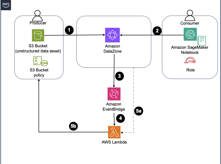


 Somdeb Bhattacharjee is a Senior Solutions Architect specializing on data and analytics. He is part of the global Healthcare and Life sciences industry at AWS, helping his customers modernize their data platform solutions to achieve their business outcomes.
 Sam Yates is a Senior Solutions Architect in the Healthcare and Life Sciences business unit at AWS. He has spent most of the past two decades helping life sciences companies apply technology in pursuit of their missions to help patients. Sam holds BS and MS degrees in Computer Science.


 Koushik Konjeti is a Senior Solutions Architect at Amazon Web Services. He has a passion for aligning architectural guidance with customer goals, ensuring solutions are tailored to their unique requirements. Outside of work, he enjoys playing cricket and tennis.


 Raks Khare is a Senior Analytics Specialist Solutions Architect at AWS based out of Pennsylvania. He helps customers across varying industries and regions architect data analytics solutions at scale on the AWS platform. Outside of work, he likes exploring new travel and food destinations and spending quality time with his family.
 Poulomi Dasgupta is a Senior Analytics Solutions Architect with AWS. She is passionate about helping customers build cloud-based analytics solutions to solve their business problems. Outside of work, she likes travelling and spending time with her family.
 Saurav Das is part of the Amazon Redshift Product Management team. He has more than 16 years of experience in working with relational databases technologies and data protection. He has a deep interest in solving customer challenges centered around high availability and disaster recovery.


 Matthias Rudolph is a Solutions Architect at AWS, digitalizing the German manufacturing industry, focusing on analytics and big data. Before that he was a lead developer at the German manufacturer KraussMaffei Technologies, responsible for the development of data platforms.
 Dipankar Mazumdar is a Staff Data Engineer Advocate at Onehouse.ai, focusing on open-source projects like Apache Hudi and XTable to help engineering teams build and scale robust analytics platforms, with prior contributions to critical projects such as Apache Iceberg and Apache Arrow.
 Stephen Said is a Senior Solutions Architect and works with Retail/CPG customers. His areas of interest are data platforms and cloud-native software engineering.


 Samir Patel is a Senior Data Architect at Amazon Web Services, where he specializes in OpenSearch, data analytics, and cutting-edge generative AI technologies. Samir works directly with enterprise customers to design and build customized solutions catered to their data analytics and cybersecurity needs. When not immersed in technical work, Samir pursues his passion for outdoor activities, including hiking, pickleball, and grilling with family and friends.
 Sesha Sanjana Mylavarapu is an Associate Data Lake Consultant at AWS Professional Services. She specializes in cloud-based data management and collaborates with enterprise clients to design and implement scalable data lakes. She has a strong interest in data analytics and enjoys assisting customers solve their business and technical challenges. Beyond her professional pursuits, Sanjana enjoys hiking, playing guitar, and is passionate about teaching yoga.
 Vivek Gautam is a Senior Data Architect with specialization in data analytics at AWS Professional Services. He works with enterprise customers building data products, analytics platforms, streaming, and search solutions on AWS. When not building and designing data products, Vivek is a food enthusiast who also likes to explore new travel destinations and go on hikes.


 Shaheer Mansoor is a Senior Machine Learning Engineer at AWS, where he specializes in developing cutting-edge machine learning platforms. His expertise lies in creating scalable infrastructure to support advanced AI solutions. His focus areas are MLOps, feature stores, data lakes, model hosting, and generative AI.
 Anoop Kumar K M is a Data Architect at AWS with focus in the data and analytics area. He helps customers in building scalable data platforms and in their enterprise data strategy. His areas of interest are data platforms, data analytics, security, file systems and operating systems. Anoop loves to travel and enjoys reading books in the crime fiction and financial domains.
 Sreenivas Nettem is a Lead Database Consultant at AWS Professional Services. He has experience working with Microsoft technologies with a specialization in SQL Server. He works closely with customers to help migrate and modernize their databases to AWS.