Customers are building databases, data warehouses, and data lake solutions in isolation from each other, each having its own separate data ingestion, storage, management, and governance layers. Often these disjointed efforts to build separate data stores end up creating data silos, data integration complexities, excessive data movement, and data consistency issues. These issues are preventing customers from getting deeper insights. To overcome these issues and easily move data around, a Lake House approach on AWS was introduced.
In this blog post, we illustrate the AWS Glue integration components that you can use to accelerate building a Lake House architecture on AWS. We will also discuss how to derive persona-centric insights from your Lake House using AWS Glue.
Components of the AWS Glue integration system
AWS Glue is a serverless data integration service that facilitates the discovery, preparation, and combination of data. It can be used for analytics, machine learning, and application development. AWS Glue provides all of the capabilities needed for data integration. So you can start analyzing your data and putting it to use in minutes, rather than months.
The following diagram illustrates the various components of the AWS Glue integration system.
Figure 1. AWS Glue integration components
Connect – AWS Glue allows you to connect to various data sources anywhere
Glue connector: AWS Glue provides built-in support for the most commonly used data stores. You can use Amazon Redshift, Amazon RDS, Amazon Aurora, Microsoft SQL Server, MySQL, MongoDB, or PostgreSQL using JDBC connections. AWS Glue also allows you to use custom JDBC drivers in your extract, transform, and load (ETL) jobs. For data stores that are not natively supported such as SaaS applications, you can use connectors. You can also subscribe to several connectors offered in the AWS Marketplace.
Glue crawlers: You can use a crawler to populate the AWS Glue Data Catalog with tables. A crawler can crawl multiple data stores in a single pass. Upon completion, the crawler creates or updates one or more tables in your Data Catalog. Extract, transform, and load (ETL) jobs that you define in AWS Glue use these Data Catalog tables as sources and targets.
Catalog – AWS Glue simplifies data discovery and governance
Glue Data Catalog: The Data Catalog serves as the central metadata catalog for the entire data landscape.
Glue Schema Registry: The AWS Glue Schema Registry allows you to centrally discover, control, and evolve data stream schemas. With AWS Glue Schema Registry, you can manage and enforce schemas on your data streaming applications.
Data quality – AWS Glue helps you author and monitor data quality rules
Glue DataBrew:AWS Glue DataBrew allows data scientists and data analysts to clean and normalize data. You can use a visual interface, reducing the time it takes to prepare data by up to 80%. With Glue DataBrew, you can visualize, clean, and normalize data directly from your data lake, data warehouses, and databases.
Curate data: You can use either Glue development endpoint or AWS Glue Studio to curate your data.
AWS Glue Studio is a new visual interface for AWS Glue that supports extract-transform-and-load (ETL) developers. You can author, run, and monitor AWS Glue ETL jobs. You can now use a visual interface to compose jobs that move and transform data, and run them on AWS Glue.
AWS Data Exchange makes it easy for AWS customers to securely exchange and use third-party data in AWS. This is for data providers who want to structure their data across multiple datasets or enrich their products with additional data. You can publish additional datasets to your products using the AWS Data Exchange.
Deequ is an open-source data quality library developed internally at Amazon, for data quality. It provides multiple features such as automatic constraint suggestions and verification, metrics computation, and data profiling.
Build a Lake House architecture faster, using AWS Glue
Figure 2 illustrates how you can build a Lake House using AWS Glue components.
Figure 2. Building Lake House architectures with AWS Glue
The architecture flow follows these general steps:
Glue crawlers scan the data from various data sources and populate the Data Catalog for your Lake House.
The Data Catalog serves as the central metadata catalog for the entire data landscape.
Once data is cataloged, fine-grained access control is applied to the tables through AWS Lake Formation.
Curate your data with business and data quality rules by using Glue Studio, Glue development endpoints, or Glue DataBrew. Place transformed data in a curated Amazon S3 for purpose built analytics downstream.
Facilitate data movement with AWS Glue to and from your data lake, databases, and data warehouse by using Glue connections. Use AWS Glue Elastic views to replicate the data across the Lake House.
Derive persona-centric insights from your Lake House using AWS Glue
Many organizations want to gather observations from increasingly larger volumes of acquired data. These insights help them make data-driven decisions with speed and agility. They must use a central data lake, a ring of purpose-built data services, and data warehouses based on persona or job function.
Figure 3 illustrates the Lake House inside-out data movement with AWS Glue DataBrew, Amazon Athena, Amazon Redshift, and Amazon QuickSight to perform persona-centric data analytics.
Figure 3. Lake House persona-centric data analytics using AWS Glue
This shows how Lake House components serve various personas in an organization:
Data processing: Data curators and data scientists use DataBrew to validate, clean, and enrich the data. Amazon Athena is also used to run improvised queries to analyze the data in the lake. The transformation is shared with data engineers to set up batch processing.
Batch data processing: Data engineers or developers set up batch jobs in AWS Glue and AWS Glue DataBrew. Jobs can be initiated by an event, or can be scheduled to run periodically.
Data analytics: Data/Business analysts can now analyze prepared dataset in Amazon Redshift or in Amazon S3 using Athena.
Data visualizations: Business analysts can create visuals in QuickSight. Data curators can enrich data from multiple sources. Admins can enforce security and data governance. Developers can embed QuickSight dashboard in applications.
Conclusion
Using a Lake House architecture will help you get persona-centric insights quickly from all of your data based on user role or job function. In this blog post, we describe several AWS Glue components and AWS purpose-built services that you can use to build Lake House architectures on AWS. We have also presented persona-centric Lake House analytics architecture using AWS Glue, to help you derive insights from your Lake House.
Read more and get started on building Lake House Architectures on AWS.
MEDHOST has been providing products and services to healthcare facilities of all types and sizes for over 35 years. Today, more than 1,000 healthcare facilities are partnering with MEDHOST and enhancing their patient care and operational excellence with its integrated clinical and financial EHR solutions. MEDHOST also offers a comprehensive Emergency Department Information System with business and reporting tools. Since 2013, MEDHOST’s cloud solutions have been utilizing Amazon Web Services (AWS) infrastructure, data source, and computing power to solve complex healthcare business cases.
MEDHOST can utilize the data available in the cloud to provide value-added solutions for hospitals solving complex problems, like predicting sepsis, cardiac risk, and length of stay (LOS) as well as reducing re-admission rates. This requires a solid foundation of data lake and elastic data pipeline to keep up with multi-terabyte data from thousands of hospitals. MEDHOST has invested a significant amount of time evaluating numerous vendors to determine the best solution for its data needs. Ultimately, MEDHOST designed and implemented machine learning/artificial intelligence capabilities by leveraging AWS Data Lab and an end-to-end data lake platform that enables a variety of use cases such as data warehousing for analytics and reporting.
Since you’re reading this post, you may also be interested in the following:
MEDHOST’s initial objectives in evaluating vendors were to:
Build a low-cost data lake solution to provide cardiac risk prediction for patients based on health records
Provide an analytical solution for hospital staff to improve operational efficiency
Implement a proof of concept to extend to other machine learning/artificial intelligence solutions
The AWS team proposed AWS Data Lab to architect, develop, and test a solution to meet these objectives. The collaborative relationship between AWS and MEDHOST, AWS’s continuous innovation, excellent support, and technical solution architects helped MEDHOST select AWS over other vendors and products. AWS Data Lab’s well-structured engagement helped MEDHOST define clear, measurable success criteria that drove the implementation of the cardiac risk prediction and analytical solution platform. The MEDHOST team consisted of architects, builders, and subject matter experts (SMEs). By connecting MEDHOST experts directly to AWS technical experts, the MEDHOST team gained a quick understanding of industry best practices and available services allowing MEDHOST team to achieve most of the success criteria at the end of a four-day design session. MEDHOST is now in the process of moving this work from its lower to upper environment to make the solution available for its customers.
Solution
For this solution, MEDHOST and AWS built a layered pipeline consisting of ingestion, processing, storage, analytics, machine learning, and reinforcement components. The following diagram illustrates the Proof of Concept (POC) that was implemented during the four-day AWS Data Lab engagement.
Ingestion layer
The ingestion layer is responsible for moving data from hospital production databases to the landing zone of the pipeline.
The hospital data was stored in an Amazon RDS for PostgreSQL instance and moved to the landing zone of the data lake using AWS Database Migration Service (DMS). DMS made migrating databases to the cloud simple and secure. Using its ongoing replication feature, MEDHOST and AWS implemented change data capture (CDC) quickly and efficiently so MEDHOST team could spend more time focusing on the most interesting parts of the pipeline.
Processing layer
The processing layer was responsible for performing extract, tranform, load (ETL) on the data to curate them for subsequent uses.
MEDHOST used AWS Glue within its data pipeline for crawling its data layers and performing ETL tasks. The hospital data copied from RDS to Amazon S3 was cleaned, curated, enriched, denormalized, and stored in parquet format to act as the heart of the MEDHOST data lake and a single source of truth to serve any further data needs. During the four-day Data Lab, MEDHOST and AWS targeted two needs: powering MEDHOST’s data warehouse used for analytics and feeding training data to the machine learning prediction model. Even though there were multiple challenges, data curation is a critical task which requires an SME. AWS Glue’s serverless nature, along with the SME’s support during the Data Lab, made developing the required transformations cost efficient and uncomplicated. Scaling and cluster management was addressed by the service, which allowed the developers to focus on cleaning data coming from homogenous hospital sources and translating the business logic to code.
Storage layer
The storage layer provided low-cost, secure, and efficient storage infrastructure.
MEDHOST used Amazon S3 as a core component of its data lake. AWS DMS migration tasks saved data to S3 in .CSV format. Crawling data with AWS Glue made this landing zone data queryable and available for further processing. The initial AWS Glue ETL job stored the parquet formatted data to the data lake and its curated zone bucket. MEDHOST also used S3 to store the .CSV formatted data set that will be used to train, test, and validate its machine learning prediction model.
Analytics layer
The analytics layer gave MEDHOST pipeline reporting and dashboarding capabilities.
The data was in parquet format and partitioned in the curation zone bucket populated by the processing layer. This made querying with Amazon Athena or Amazon Redshift Spectrum fast and cost efficient.
From the Amazon Redshift cluster, MEDHOST created external tables that were used as staging tables for MEDHOST data warehouse and implemented an UPSERT logic to merge new data in its production tables. To showcase the reporting potential that was unlocked by the MEDHOST analytics layer, a connection was made to the Redshift cluster to Amazon QuickSight. Within minutes MEDHOST was able to create interactive analytics dashboards with filtering and drill-down capabilities such as a chart that showed the number of confirmed disease cases per US state.
Machine learning layer
The machine learning layer used MEDHOST’s existing data sets to train its cardiac risk prediction model and make it accessible via an endpoint.
Before getting into Data Lab, the MEDHOST team was not intimately familiar with machine learning. AWS Data Lab architects helped MEDHOST quickly understand concepts of machine learning and select a model appropriate for its use case. MEDHOST selected XGBoost as its model since cardiac prediction falls within regression technique. MEDHOST’s well architected data lake enabled it to quickly generate training, testing, and validation data sets using AWS Glue.
Amazon SageMaker abstracted underlying complexity of setting infrastructure for machine learning. With few clicks, MEDHOST started Jupyter notebook and coded the components leading to fitting and deploying its machine learning prediction model. Finally, MEDHOST created the endpoint for the model and ran REST calls to validate the endpoint and trained model. As a result, MEDHOST achieved the goal of predicting cardiac risk. Additionally, with Amazon QuickSight’s SageMaker integration, AWS made it easy to use SageMaker models directly in visualizations. QuickSight can call the model’s endpoint, send the input data to it, and put the inference results into the existing QuickSight data sets. This capability made it easy to display the results of the models directly in the dashboards. Read more about QuickSight’s SageMaker integration here.
Reinforcement layer
Finally, the reinforcement layer guaranteed that the results of the MEDHOST model were captured and processed to improve performance of the model.
The MEDHOST team went beyond the original goal and created an inference microservice to interact with the endpoint for prediction, enabled abstracting of the machine learning endpoint with the well-defined domain REST endpoint, and added a standard security layer to the MEDHOST application.
When there is a real-time call from the facility, the inference microservice gets inference from the SageMaker endpoint. Records containing input and inference data are fed to the data pipeline again. MEDHOST used Amazon Kinesis Data Streams to push records in real time. However, since retraining the machine learning model does not need to happen in real time, the Amazon Kinesis Data Firehose enabled MEDHOST to micro-batch records and efficiently save them to the landing zone bucket so that the data could be reprocessed.
Conclusion
Collaborating with AWS Data Lab enabled MEDHOST to:
Store single source of truth with low-cost storage solution (data lake)
Complete data pipeline for a low-cost data analytics solution
Create an almost production-ready code for cardiac risk prediction
The MEDHOST team learned many concepts related to data analytics and machine learning within four days. AWS Data Lab truly helped MEDHOST deliver results in an accelerated manner.
About the Authors
Pandian Velayutham is the Director of Engineering at MEDHOST. His team is responsible for delivering cloud solutions, integration and interoperability, and business analytics solutions. MEDHOST utilizes modern technology stack to provide innovative solutions to our customers. Pandian Velayutham is a technology evangelist and public cloud technology speaker.
George Komninos is a Data Lab Solutions Architect at AWS. He helps customers convert their ideas to a production-ready data product. Before AWS, he spent 3 years at Alexa Information domain as a data engineer. Outside of work, George is a football fan and supports the greatest team in the world, Olympiacos Piraeus.
If you use data lakes in Amazon Simple Storage Service (Amazon S3) and use SAP HANA as your transactional data store, you may need to join the data in your data lake with SAP HANA in the cloud, SAP HANA running on Amazon Elastic Compute Cloud (Amazon EC2), or with an on-premises SAP HANA, for example to build a dashboard or create consolidated reporting.
In such use cases, Amazon Athena Federated Query allows you to seamlessly access the data from SAP HANA database without building ETL pipelines to copy or unload the data to the S3 data lake or SAP HANA. This removes the overhead of creating additional extract, transform, and load (ETL) processes and shortens the development cycle.
In this post, we walk you through a step-by-step configuration to set up Amazon Athena Federated Query using AWS Lambda to access data in a SAP HANA database running on AWS.
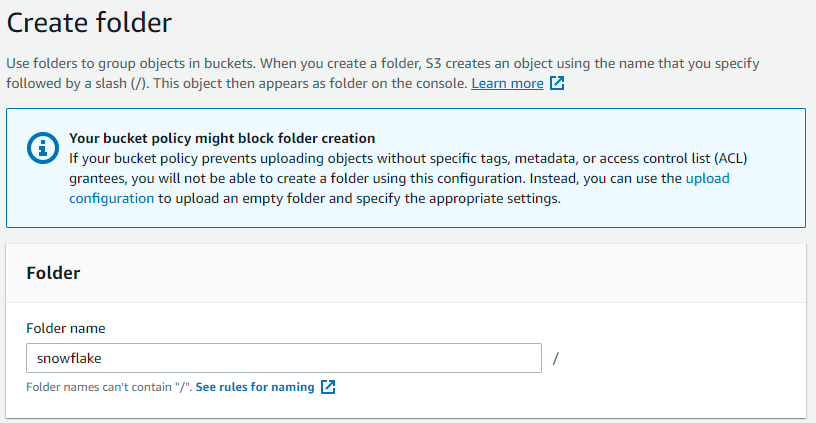
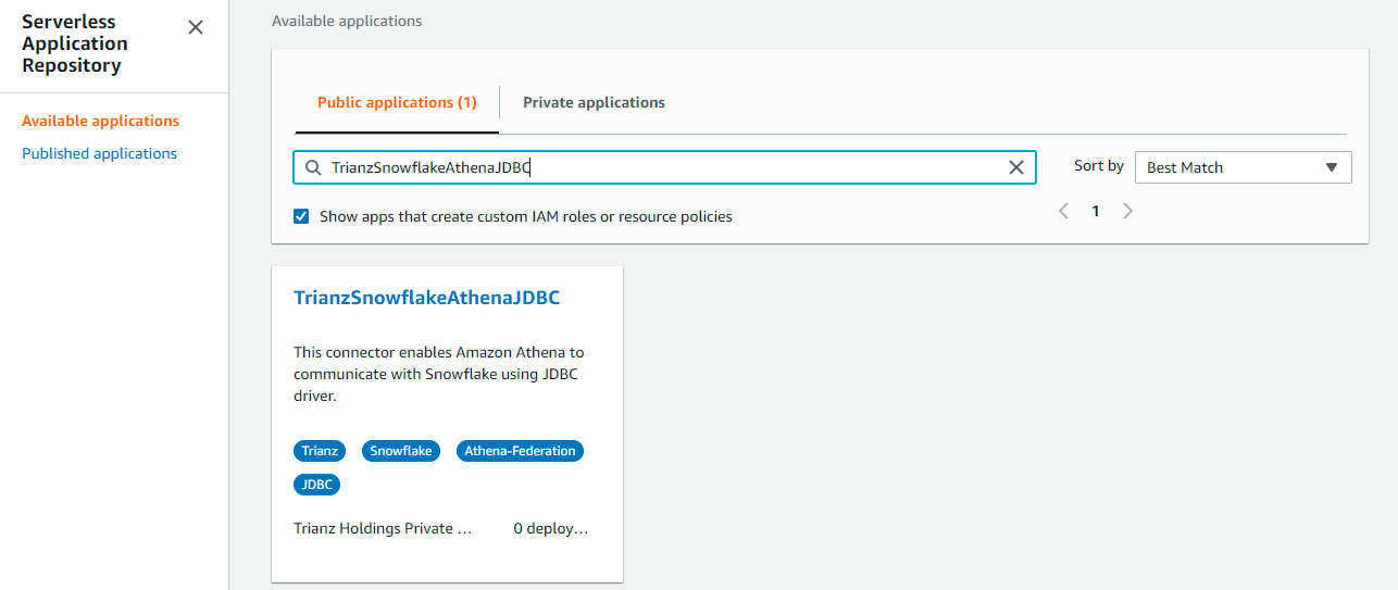
For this post, we will be using the SAP HANA Athena Federated query connector developed by Trianz. You can deploy the Athena Federated query connector developed by Trianz available in the AWS Serverless Application Repository.
Let’s start with discussing the solution and then detailing the steps involved.
Solution overview
Data federation is the capability to integrate data in another data store using a single interface (Athena). The following diagram depicts how Athena federation works by using Lambda to integrate with a federated data source.
Athena is an interactive query service that makes it easy to analyze data in Amazon S3 using standard SQL. If you have data in sources other than Amazon S3, you can use Athena Federated Query to query the data in place or build pipelines to extract data from multiple data sources and store them in Amazon S3. With Athena Federated Query, you can run SQL queries across data stored in relational, non-relational, object, and custom data sources.
When a federated query is run, Athena identifies the parts of the query that should be routed to the data source connector and executes them with Lambda. The data source connector makes the connection to the source, runs the query, and returns the results to Athena. If the data doesn’t fit into Lambda RAM runtime memory, it spills the data to Amazon S3 and is later accessed by Athena.
Athena uses data source connectors which internally use Lambda to run federated queries. Data source connectors are pre-built and can be deployed from the Athena console or from the Serverless Application Repository. Based on the user submitting the query, connectors can provide or restrict access to specific data elements.
To implement this solution, we complete the following steps:
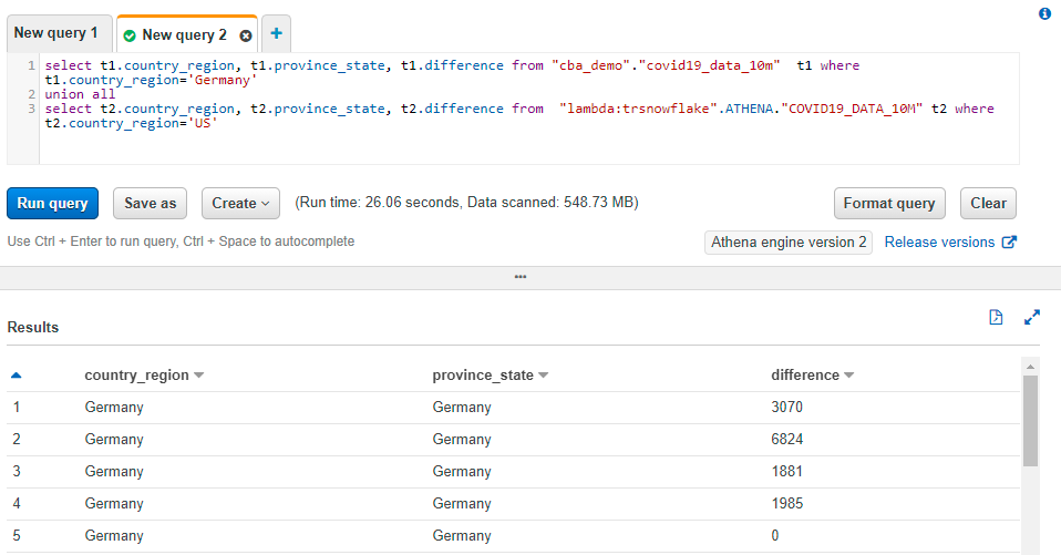
Run your federated queries using lambda:trsaphana to run against tables in the SAP HANA database. trsaphana is the name of lambda function which we have created in step 7 of previous section of this blog.
lambda:trsaphana is a reference data source connector Lambda function using the format lambda:MyLambdaFunctionName. For more information, see Writing Federated Queries.
The following screenshot demonstrates joining the dataset between SAP HANA and the data lake.
Key performance best practice considerations
If you’re considering Athena federation with a SAP HANA database, we recommend the following best practices:
Athena federation works great for queries with predicate filtering because the predicates are pushed down to the SAP HANA database. Use filter and limited-range scans in your queries to avoid full table scans.
If your SQL query requires returning a large volume of data from the SAP HANA database to Athena (which could lead to query timeouts or slow performance), unload the large tables in your query from SAP HANA to your S3 data lake.
Star schema is a commonly used data model in SAP HANA databases. In the star schema model, unload your large fact tables into your S3 data lake and leave the dimension tables in your SAP HANA database. If large dimension tables are contributing to slow performance or query timeouts, unload those tables to your S3 data lake.
When you run federated queries, Athena spins up multiple Lambda functions, which causes a spike in database connections. It’s important to monitor the SAP HANA database WLM queue slots to ensure there is no queuing. Additionally, you can use concurrency scaling on your SAP HANA database cluster to benefit from concurrent connections to queue up.
Conclusion
In this post, you learned how to configure and use Athena Federated query with SAP HANA using Lambda. Now you don’t need to wait for all the data in your SAP HANA data warehouse to be unloaded to Amazon S3 and maintained on a day-to-day basis to run your queries.
You can use the best practice considerations outlined in the post to help minimize the data transferred from SAP HANA for better performance. When queries are well-written for Federated query, the performance penalties are negligible.
Navnit Shukla is AWS Specialist Solution Architect in Analytics. He is passionate about helping customers uncover insights from their data. He has been building solutions to help organizations make data-driven decisions.
This blog post is co-written by Russell Harlin from Comcast Corporation.
Comcast Corporation creates incredible technology and entertainment that connects millions of people to the moments and experiences that matter most. At the core of this is Comcast’s high-speed data network, providing tens of millions of customers across the country with reliable internet connectivity. This mission has become more important now than ever.
This post walks through how Comcast used AWS to rapidly store and analyze large-scale telemetry data.
Background
At Comcast, we’re constantly looking for ways to gain new insights into our network and improve the overall quality of service. Doing this effectively can involve scaling solutions to support analytics across our entire network footprint. For this particular project, we wanted an extensible and scalable solution that could process, store, and analyze telemetry reports, one per network device every 5 minutes. This data would then be used to help measure quality of experience and determine where network improvements could be made.
Scaling big data solutions is always challenging, but perhaps the biggest challenge of this project was the accelerated timeline. With 2 weeks to deliver a prototype and an additional month to scale it, we knew we couldn’t go through the traditional bake-off of different technologies, so we had to either go with technologies we were comfortable with or proven managed solutions.
For the data streaming pipeline, we already had the telemetry data coming in on an Apache Kafka topic, and had significant prior experience using Kafka combined with Apache Flink to implement and scale streaming pipelines, so we decided to go with what we knew. For the data storage and analytics, we needed a suite of solutions that could scale quickly, had plenty of support, and had an ecosystem of well-integrated tools to solve any problem that might arise. This is where AWS was able to meet our needs with technologies like Amazon Simple Storage Service (Amazon S3), AWS Glue, Amazon Athena, and Amazon Redshift.
Initial architecture
Our initial prototype architecture for the data store needed to be fast and simple so that we could unblock the development of the other elements of the budding telemetry solution. We needed three key things out of it:
The ability to easily fetch raw telemetry records and run more complex analytical queries
The capacity to integrate seamlessly with the other pieces of the pipeline
The possibility that it could serve as a springboard to a more scalable long-term solution
The first instinct was to explore solutions we used in the past. We had positive experiences with using nosql databases, like Cassandra, to store and serve raw data records, but it was clear these wouldn’t meet our need for running ad hoc analytical queries. Likewise, we had experience with more flexible RDBMs, like Postgres, for handling more complicated queries, but we knew that those wouldn’t scale to meet our requirement to store tens to hundreds of billions of rows. Therefore, any prototyping with one of these approaches would be considered throwaway work.
After moving on from these solutions, we quickly settled on using Amazon S3 with Athena. Amazon S3 provides low-cost storage with near-limitless scaling, so we knew we could store as much historical data as required and Athena would provide serverless, on-demand querying of our data. Additionally, Amazon S3 is known to be a launching pad to many other data store solutions both inside and outside the AWS ecosystem. This was perfect for the exploratory prototyping phase.
Integrating it into the rest of our pipeline would also prove simple. Writing the data to Amazon S3 from our Flink job was straightforward and could be done using the readily available Flink streaming file sink with an Amazon S3 bucket as the destination. When the data was available in Amazon S3, we ran AWS Glue to index our Parquet-formatted data and generate schemas in the AWS Glue metastore for searching using Athena with standard SQL.
The following diagram illustrates this architecture.
Using Amazon S3 and Athena allowed us to quickly unblock development of our Flink pipeline and ensure that the data being passed through was correct. Additionally, we used the AWS SDK to connect to Athena from our northbound Golang microservice and provide REST API access to our data for our custom web application. This allowed us to prove out an end-to-end solution with almost no upfront cost and very minimal infrastructure.
Updated architecture
As application and service development proceeded, it became apparent that Amazon Athena performed for developers running ad hoc queries, but wasn’t going to work as a long-term responsive backend for our microservices and user interface requirements.
One of the primary use cases of this solution was to look at device-level telemetry reports for a period of time and plot and track different aspects of their quality of experience. Because this most often involves solving problems happening in the now, we needed an improved data store for the most recent hot data.
This led us to Amazon Redshift. Amazon Redshift requires loading the data into a dedicated cluster and formulating a schema tuned for your use cases.
The following diagram illustrates this updated architecture.
Data loading and storage requirements
For loading and storing the data in Amazon Redshift, we had a few fundamental requirements:
Because our Amazon Redshift solution would be for querying data to troubleshoot problems happening as recent as the current hour, we needed to minimize the latency of the data load and keep up with our scale while doing it. We couldn’t live with nightly loads.
The pipeline had to be robust and recover from failures automatically.
There’s a lot of nuance that goes into making this happen, and we didn’t want to worry about handling these basic things ourselves, because this wasn’t where we were going to add value. Luckily, because we were already loading the data into Amazon S3, AWS Glue ETL satisfied these requirements and provided a fast, reliable, and scalable solution to do periodic loads from our Amazon S3 data store to our Amazon Redshift cluster.
A huge benefit of AWS Glue ETL is that it provides many opportunities to tune your ETL pipeline to meet your scaling needs. One of our biggest challenges was that we write multiple files to Amazon S3 from different regions every 5 minutes, which results in many small files. If you’re doing infrequent nightly loads, this may not pose a problem, but for our specific use case, we wanted to load data at least every hour and multiple times an hour if possible. This required some specific tuning of the default ETL job:
Amazon S3 list implementation – This allows the Spark job to handle files in batches and optimizes reads for a large number of files, preventing out of memory issues.
Pushdown predicates – This tells the load to skip listing any partitions in Amazon S3 that you know won’t be a part of the current run. For frequent loads, this can mean skipping a lot of unnecessary file listing during each job run.
File grouping – This allows the read from Amazon S3 to group files together in batches when reading from Amazon S3. This greatly improves performance when reading from a large number of small files.
AWS Glue 2.0 – When we were starting our development, only AWS Glue 1.0 was available, and we’d frequently see Spark cluster start times of over 10 minutes. This becomes problematic if you want to run the ETL job more frequently because you have to account for the cluster startup time in your trigger timings. When AWS Glue 2.0 came out, those start times consistently dropped to under 1 minute and they became a afterthought.
With these tunings, as well as increasing the parallelism of the job, we could meet our requirement of loading data multiple times an hour. This made relevant data available for analysis sooner.
Modeling, distributing, and sorting the data
Aside from getting the data into the Amazon Redshift cluster in a timely manner, the next consideration was how to model, distribute, and sort the data when it was in the cluster. For our data, we didn’t have a complex setup with tens of tables requiring extensive joins. We simply had two tables: one for the device-level telemetry records and one for records aggregated at a logical grouping.
The bulk of the initial query load would be centered around serving raw records from these tables to our web application. These types of raw record queries aren’t difficult to handle from a query standpoint, but do present challenges when dealing with tens of millions of unique devices and a report granularity of 5 minutes. So we knew we had to tune the database to handle these efficiently. Additionally, we also needed to be able to run more complex ad hoc queries, like getting daily summaries of each table so that higher-level problem areas could be more easily tracked and spotted in the network. These queries, however, were less time sensitive and could be run on an ad hoc, batch-like basis where responsiveness wasn’t as important.
The schema fields themselves were more or less one-to-one mappings from the respective Parquet schemas. The challenge came, however, in picking partition keys and sorting columns. For partition keys, we identified a logical device grouping column present in both our tables as the one column we were likely to join on. This seemed like a natural fit to partition on and had good enough cardinality that our distribution would be adequate.
For the sorting keys, we knew we’d be searching by the device identifier and the logical grouping; for the respective tables, and we knew we’d be searching temporally. So the primary identifier column of each table and the timestamp made sense to sort on. The documented sort key order suggestion was to use the timestamp column as the first value in the sort key, because it could provide dataset filtering on a specific time period. This initially worked well enough and we were able to get a performance improvement over Athena, but as we scaled and added more data, our raw record retrieval queries were rapidly slowing down. To help with this, we made two adjustments.
The first adjustment came with a change to the sort key. The first part of this involved swapping the order of the timestamp and the primary identifier column. This allowed us to filter down to the device and then search through the range of timestamps on just that device, skipping over all irrelevant devices. This provided significant performance gains and cut our raw record query times by several multiples. The second part of the sort key adjustment involved adding another column (a node-level identifier) to the beginning of the sort key. This allowed us to have one more level of data filtering, which further improved raw record query times.
One trade-off made while making these sort key adjustments was that our more complex aggregation queries had a noticeable decline in performance. This was because they were typically run across the entire footprint of devices and could no longer filter as easily based on time being the first column in the sort key. Fortunately, because these were less frequent and could be run offline if necessary, this performance trade-off was considered acceptable.
If the frequency of these workloads increases, we can use materialized views in Amazon Redshift, which can help avoid unnecessary reruns of the complex aggregations if minimal-to-no data changes in the underlying base tables have occurred since the last run.
The final adjustment was cluster scaling. We chose to use the Amazon Redshift next-generation RA3 nodes for a number of benefits, but three especially key benefits:
RA3 clusters allow for practically unlimited storage in our cluster.
The RA3 ability to scale storage and compute independently paired really well with our expectations and use cases. We fully expected our Amazon Redshift storage footprint to continue to grow, as well as the number, shape, and sizes of our use cases and users, but data and workloads wouldn’t necessarily grow in lockstep. Being able to scale the cluster’s compute power independent of storage (or vice versa) was a key technical requirement and cost-optimization for us.
RA3 clusters come with Amazon Redshift managed storage, which places the burden on Amazon Redshift to automatically situate data based on its temperature for consistently peak performance. With managed storage, hot data was cached on a large local SSD cache in each node, and cold data was kept in the Amazon Redshift persistent store on Amazon S3.
After conducting performance benchmarks, we determined that our cluster was under-powered for the amount of data and workloads it was serving, and we would benefit from greater distribution and parallelism (compute power). We easily resized our Amazon Redshift cluster to double the number of nodes within minutes, and immediately saw a significant performance boost. With this, we were able to recognize that as our data and workloads scaled, so too should our cluster.
Looking forward, we expect that there will be a relatively small population of ad hoc and experimental workloads that will require access to additional datasets sitting in our data lake, outside of Amazon Redshift in our data lake—workloads similar to the Athena workloads we previously observed. To serve that small customer base, we can leverage Amazon Redshift Spectrum, which empowers users to run SQL queries on external tables in our data lake, similar to SQL queries on any other table within Amazon Redshift, while allowing us to keep costs as lean as possible.
This final architecture provided us with the solid foundation of price, performance, and flexibility for our current set of analytical use cases—and, just as important, the future use cases that haven’t shown themselves yet.
Summary
This post details how Comcast leveraged AWS data store technologies to prototype and scale the serving and analysis of large-scale telemetry data. We hope to continue to scale the solution as our customer base grows. We’re currently working on identifying more telemetry-related metrics to give us increased insight into our network and deliver the best quality of experience possible to our customers.
About the Authors
Russell Harlin is a Senior Software Engineer at Comcast based out of the San Francisco Bay Area. He works in the Network and Communications Engineering group designing and implementing data streaming and analytics solutions.
Asser Moustafa is an Analytics Specialist Solutions Architect at AWS based out of Dallas, Texas. He advises customers in the Americas on their Amazon Redshift and data lake architectures and migrations, starting from the POC stage to actual production deployment and maintenance
Amit Kalawat is a Senior Solutions Architect at Amazon Web Services based out of New York. He works with enterprise customers as they transform their business and journey to the cloud.
Today’s modern applications use multiple purpose-built database engines, including relational, key-value, document, and in-memory databases. This purpose-built approach improves the way applications use data by providing better performance and reducing cost. However, the approach raises some challenges for data teams that need to provide a holistic view on top of these database engines, and especially when they need to merge the data with datasets in the organization’s data lake.
For our use case, assume you’re operating a fleet of scooters, and need to forecast whether enough scooters are made available in each part of the city. Specifically, you need to predict the number of scooters needed in each urban neighborhood for the upcoming hour. You have a pre-trained ML model that forecasts the demand for the next hour based on data from the past 4 hours. You use Athena and Amazon QuickSight to predict and visualize the demand, respectively.
Solution overview
The following diagram shows the overall architecture of our solution.
Populate DynamoDB with data and create a SageMaker endpoint to query in Athena
For this post, we populate the DynamoDB table with scooter data. For demand prediction, we create a new SageMaker endpoint using a pre-trained XGBoost model using an elastic container registry path from Region us-east-1.
Choose Launch Stack to launch a CloudFormation stack in us-east-1.
On the CloudFormation console, accept default values for the parameters.
Select I acknowledge that AWS CloudFormation might create IAM resources with custom names.
Choose Create stack.
The stack creates five resources:
A DynamoDB table
A Lambda function to load the table with relevant data
A SageMaker endpoint for inference requests, with the pre-trained XGBoost model from an Amazon Simple Storage Service (Amazon S3) location
An Athena workgroup named V2EngineWorkGroup
Named Athena queries to look up the shapefiles and predict the demand for scooters
It can take up to 15–20 minutes for the CloudFormation stack to create these resources.
You can verify the sample data provided by AWS CloudFormation was loaded into DynamoDB by navigating to the DynamoDB console and checking for the table DynamoDBTableDocklessVehicles.
When resource creation is complete, on the Athena console, choose Workgroups.
Select the workgroup V2EngineWorkGroup and choose Switch workgroup.
If you get a prompt to save the query result location, choose an S3 location where you have write permissions.
Choose Save.
In the Athena query editor, select the database athena-ml-db-<your-AWS-Account-Number>.
Now let’s load the geolocation files into the Athena database.
Create an Athena table with geospatial data of neighborhood boundaries
To load the geolocation files into Athena, complete the following steps:
On the Athena console, choose Saved queries.
Search for and select Q1: Neighborhoods.
Return to the Athena SQL window.
This query creates a new table for the geospatial data that represents the urban neighborhoods of the city. The data table has been created from GIS shapefiles. The following CREATE EXTERNAL TABLE statement defines the schema of the table, and the location and format of the underlying data file. You can find the Python code to process shapefiles and produce this table in the notebook Geo-Spatial processing of GIS shapefiles with Amazon Athena.
--------- Start SQL -----
-- Q1: Neighborhoods
-- -----------------
-- This Athena statement creates a table entry in the Glue catalog
-- The data format is a TAB-seperated text file without header row
--
CREATE EXTERNAL TABLE "<Here goes your Athena database>"."louisville_ky_neighborhoods"
(
    `objectid` int,
    `nh_code` int,
    `nh_name` string,
    `shapearea` double,
    `shapelen` double,
    `bb_west` double,
    `bb_south` double,
    `bb_east` double,
    `bb_north` double,
    `shape` string,
    `cog_longitude` double,
    `cog_latitude` double)
ROW FORMAT DELIMITED
 FIELDS TERMINATED BY '\t'
 LINES TERMINATED BY '\n'
STORED AS INPUTFORMAT 'org.apache.hadoop.mapred.TextInputFormat'
OUTPUTFORMAT 'org.apache.hadoop.hive.ql.io.HiveIgnoreKeyTextOutputFormat'
LOCATION 's3://<Here goes your S3 bucket>/louisville_ky_neighborhoods/'
TBLPROPERTIES (
    'has_encrypted_data'='false'
)
--------- End SQL -----
Choose Run query or press CTRL+Enter.
This action creates a table named louisville_ky_neighborhoods in your database. Make sure the table is created in the database athena-ml-db-<your-AWS-Account-Number>.
Predict demand for scooters by neighborhood from the aggregated DynamoDB data
Now you can use Athena to query transactional data directly from DynamoDB, and aggregate it for analysis and forecast. This feature isn’t easily achieved by directly querying a DynamoDB NoSQL database.
On the Athena console, choose Saved queries.
Search for and select Q2: DynamoDBAthenaMLScooterPredict.
Return to the Athena SQL window.
This SQL statement demonstrates the use of the Athena Query Federation to query the DyanamoDB table with the raw trip data, Athena’s geospatial functions to place geographic coordinates into neighborhoods, and enrich data with ML inference using SageMaker.
The first part of the SQL statement declares the external function to query ML inferences from the SageMaker endpoint that hosts the pre-trained model. We need to define the order and type of the input parameters and the type of the return values.
We use several sub-queries to build the feature table for ML prediction. With the first SELECT statement, we query the raw data from DynamoDB for a given window. Then we locate the start and end locations of each trip record within their urban neighborhoods. Next, we create two aggregations over time and space for the start and end of the trips and combine them to generate a table with the number of trips per hour that started and ended within each of the neighborhoods. Among a few other parameters, we use the hourly counts for the past 4 hours to predict the demand for vehicles for the next hour. You can find the Python code for training the ML model in the notebook Demand Prediction for scooters using Amazon SageMaker and Amazon Athena.
--------------- Start SQL------
-- Q2: DynamoDBAthenaMLScooterPredict
-- ----------------------------------
-- Query demand of scooters for the next hour
--
-- Define function to represent the SageMaker model and endpoint for the prediction
USING EXTERNAL FUNCTION predict_demand( location_id BIGINT, hr BIGINT , dow BIGINT,
 n_pickup_1 BIGINT, n_pickup_2 BIGINT, n_pickup_3 BIGINT, n_pickup_4 BIGINT,
 n_dropoff_1 BIGINT, n_dropoff_2 BIGINT, n_dropoff_3 BIGINT, n_dropoff_4 BIGINT
 )
 RETURNS DOUBLE SAGEMAKER '<Here goes your SageMaker endpoint>'
-- query raw trip data from DynamoDB, we only need the past five hours (i.e. 5 hour time window ending with the time we set as current time)
WITH trips_raw AS (
    SELECT *
    , from_unixtime(start_epoch) AS t_start
    , from_unixtime(end_epoch) AS t_end
    FROM "lambda:<Here goes your DynamoDB connector>"."<Here goes your database>"."<Here goes your DynamoDB table>" dls
      WHERE start_epoch BETWEEN to_unixtime(TIMESTAMP '2019-09-07 15:00' - interval '5' hour) AND to_unixtime(TIMESTAMP '2019-09-07 15:00')
          OR end_epoch BETWEEN to_unixtime(TIMESTAMP '2019-09-07 15:00' - interval '5' hour) AND to_unixtime(TIMESTAMP '2019-09-07 15:00')
),
-- prepare individual trip records
trips AS (
    SELECT tr.*
        , nb1.nh_code AS start_nbid
        , nb2.nh_code AS end_nbid
        , floor( ( tr.start_epoch - to_unixtime(TIMESTAMP '2019-09-07 15:00' - interval '5' hour) )/3600 ) AS t_hour_start
        , floor( ( tr.end_epoch - to_unixtime(TIMESTAMP '2019-09-07 15:00' - interval '5' hour) )/3600 ) AS t_hour_end
    FROM trips_raw tr
    JOIN "AwsDataCatalog"."<Here goes your Athena database >"."louisville_ky_neighborhoods" nb1
        ON ST_Within(ST_POINT(CAST(tr.startlongitude AS DOUBLE), CAST(tr.startlatitude AS DOUBLE)), ST_GeometryFromText(nb1.shape))
    JOIN "AwsDataCatalog"."< Here goes your Athena database >"."louisville_ky_neighborhoods" nb2
        ON ST_Within(ST_POINT(CAST(tr.endlongitude AS DOUBLE), CAST(tr.endlatitude AS DOUBLE)), ST_GeometryFromText(nb2.shape))
),
-- aggregating trips over start time and start neighborhood
start_count AS (
    SELECT start_nbid AS nbid, COUNT(start_nbid) AS n_total_start
        , SUM(CASE WHEN t_hour_start=1 THEN 1 ELSE 0 END) AS n1_start
        , SUM(CASE WHEN t_hour_start=2 THEN 1 ELSE 0 END) AS n2_start
        , SUM(CASE WHEN t_hour_start=3 THEN 1 ELSE 0 END) AS n3_start
        , SUM(CASE WHEN t_hour_start=4 THEN 1 ELSE 0 END) AS n4_start
    FROM trips
        WHERE start_nbid BETWEEN 1 AND 98
    GROUP BY start_nbid
),
-- aggregating trips over end time and end neighborhood
end_count AS (
    SELECT end_nbid AS nbid, COUNT(end_nbid) AS n_total_end
        , SUM(CASE WHEN t_hour_end=1 THEN 1 ELSE 0 END) AS n1_end
        , SUM(CASE WHEN t_hour_end=2 THEN 1 ELSE 0 END) AS n2_end
        , SUM(CASE WHEN t_hour_end=3 THEN 1 ELSE 0 END) AS n3_end
        , SUM(CASE WHEN t_hour_end=4 THEN 1 ELSE 0 END) AS n4_end
    FROM trips
    WHERE end_nbid BETWEEN 1 AND 98
    GROUP BY end_nbid
),
-- call the predictive model to get the demand forecast for the next hour
predictions AS (
    SELECT sc.nbid
        , predict_demand(
        CAST(sc.nbid AS BIGINT),
        hour(TIMESTAMP '2019-09-07 15:00'),
        day_of_week(TIMESTAMP '2019-09-07 15:00'),
        sc.n1_start, sc.n2_start, sc.n3_start, sc.n4_start,
        ec.n1_end, ec.n2_end, ec.n3_end, ec.n4_end
        ) AS n_demand
    FROM start_count sc
    JOIN end_count ec
      ON sc.nbid=ec.nbid
)
-- finally join the predicted values with the neighborhoods' meta data
SELECT nh.nh_code AS nbid, nh.nh_name AS neighborhood, nh.cog_longitude AS longitude, nh.cog_latitude AS latitude
    , ST_POINT(nh.cog_longitude, nh.cog_latitude) AS geo_location
    , COALESCE( round(predictions.n_demand), 0 ) AS demand
FROM "AwsDataCatalog"."< Here goes your Athena database >"."louisville_ky_neighborhoods" nh
LEFT JOIN predictions
    ON nh.nh_code=predictions.nbid

    --------------- End SQL------
Choose Run query or press CTRL+Enter to run the query and predict the demand for scooters.
The output table includes the neighborhood, longitude and latitude of the centroid of the neighborhood, and the number of vehicles that are predicted for the next hour. This query produces the predictions for a selected point in time. You can make predictions for any other time by changing the expression TIMESTAMP '2019-09-07 15:00' everywhere in the statement. Change it to NOW()if you have a real-time data feed from your DynamoDB table.
Visualize predicted demand for scooters in QuickSight
You can use the same Athena query (Q2) to visualize the data in QuickSight. You may have to add additional permissions to your QuickSight role to invoke Lambda functions to access the DynamoDB tables and SageMaker endpoints for the predictions. For detailed instructions on how to set up QuickSight to visualize geo-location coordinates, see the GitHub repo.
As you can see in the following QuickSight visualization, we can spot the demand for scooters on the map of Louisville, Kentucky. Circles with a bigger radius denote higher demand for scooters in that neighborhood. You can also hover over any of the circles to view the detailed demand count and the name of the neighborhood.
Sachin Doshi is a Senior Application Architect working in the AWS Professional Services team. He is based out of New York metropolitan area. Sachin helps customers optimize their applications using cloud native AWS services.
Péter Molnár is a Data Scientist with AWS Professional Services. He develops machine learning and artificial intelligence solutions for customer business problems. He holds a doctorate in Theoretical Physics from the University of Stuttgart (Germany) and a master’s degree in Physics from Georgia Augusta University in Göttingen (Germany).
The global retail market continues to grow larger and the influx of consumer data increases daily. The rise in volume, variety, and velocity of data poses challenges with demand forecasting and inventory planning. Outdated systems generate inaccurate demand forecasts. This results in multiple challenges for retailers. They are faced with over-stocking and lost sales, and often have to rely on increased levels of safety stock to avoid losing sales.
A recent McKinsey study indicates that AI-based forecasting improves forecasting accuracy by 10–20 percent. This translates to revenue increases of 2–3 percent. An accurate forecasting system can also help determine ideal inventory levels and better predict the impact of sales promotions. It provides a single view of demand across all channels and a better customer experience overall.
In this blog post, we will show you how to build a reliable retail forecasting system. We will use Amazon Forecast, and an AWS-vetted solution called Improving Forecast Accuracy with Machine Learning. This is an AWS Solutions Implementation that automatically produces forecasts and generates visualization dashboards. This solution can be extended to use cases across a variety of industries.
Improving Forecast Accuracy solution architecture
This post will illustrate a retail environment that has an SAP S/4 HANA system for overall enterprise resource planning (ERP). We will show a forecasting solution based on Amazon Forecast to predict demand across product categories. The environment also has a unified platform for customer experience provided by SAP Customer Activity Repository (CAR). Replenishment processes are driven by SAP Forecasting and Replenishment (F&R), and SAP Fiori apps are used to manage forecasts.
The solution is divided into four parts: Data extraction and preparation, Forecasting and monitoring, Data visualization, and Forecast import and utilization in SAP.
Figure 1. Notional architecture for improving forecasting accuracy solution and SAP integration
Related data that can potentially affect demand levels can be uploaded to Amazon S3. These could include seasonal events, promotions, and item price. Additional item metadata, such as product descriptions, color, brand, size may also be uploaded. Amazon Forecast provides built-in related time series data for holidays and weather. These three components together form the forecast inputs.
Forecasting and monitoring
An S3 event notification will be initiated when new datasets are uploaded to the input bucket. This in turn, starts an AWS Step Functions state machine. The state machine combines a series of AWS Lambda functions that build, train, and deploy machine learning models in Amazon Forecast. All AWS Step Functions logs are sent to Amazon CloudWatch. Administrators will be notified with the results of the AWS Step Functions through Amazon Simple Notification Service (SNS).
An AWS Glue job combines raw forecast input data, metadata, predictor backtest exports, and forecast exports. These all go into an aggregated view of forecasts in an S3 bucket. It is then translated to the format expected by the External Forecast import interface. Amazon Athena can be used to query forecast output in S3 using standard SQL queries.
Data visualization
Amazon QuickSight analyses can be created on a per-forecast basis. This provides users with forecast output visualization across hierarchies and categories of forecasted items. It also displays item-level accuracy metrics. Dashboards can be created from these analyses and shared within the organization. Additionally, data scientists and developers can prepare and process data, and evaluate Forecast outputs using an Amazon SageMaker Notebook Instance.
Forecast import and utilization in SAP
Amazon Forecast outputs located in Amazon S3 will be imported into the Unified Demand Forecast (UDF) module within the SAP Customer Activity Repository (CAR). You can read here about how to import external forecasts. An AWS Lambda function will be initiated when aggregated forecasts are uploaded to the S3 bucket. The Lambda function performs a remote function call (RFC) to the SAP system through the official SAP JCo Library. The SAP RFC credentials and connection information may be stored securely inside AWS Secrets Manager and read on demand to establish connectivity.
Once imported, forecast values from the solution can be retrieved by SAP Forecasting and Replenishment (F&R). They will be consumed as an input to replenishment processes, which consist of requirements calculation and requirement quantity optimization. SAP F&R calculates requirements based on the forecast, the current stock, and the open purchase orders. The requirement quantity then may be improved in accordance with optimization settings defined in SAP F&R.
To illustrate how beneficial this solution can be for retail organizations, let’s consider AnyCompany Stores, Inc. This is a hypothetical customer and leader in the retailer industry with 985 stores across the United States. They struggle with issues stemming from their existing forecasting implementation. That implementation only understands certain categories and does not factor in the entire product portfolio. Additionally, it is limited to available demand history and does not consider related information that may affect forecasts. AnyCompany Stores is looking to improve their demand forecasting system.
Using Improving Forecast Accuracy with Machine Learning, AnyCompany Stores can easily generate AI-based forecasts at appropriate quantiles to address sensitivities associated with respective product categories. This mitigates inconsistent inventory buys, overstocks, out-of-stocks, and margin erosion. The solution also considers all relevant related data in addition to the historical demand data. This ensures that generated forecasts are accurate for each product category.
The generated forecasts may be used to complement existing forecasting and replenishment processes. With an improved forecasting solution, AnyCompany Stores will be able to meet demand, while holding less inventory and improving customer experience. This also helps ensure that potential demand spikes are accurately captured, so staples will always be in stock. Additionally, the company will not overstock expensive items with short shelf lives that are likely to spoil.
Conclusion
In this post, we explored how to implement an accurate retail forecasting solution using a ready-to-deploy AWS Solution. We use generated forecasts to drive inventory replenishment optimization and improve customer experience. The solution can be extended to inventory, workforce, capacity, and financial planning.
We showcase one of the ways in which Improving Forecast Accuracy with Machine Learning may be extended for a use case in the retail industry. If your organization would like to improve business outcomes with the power of forecasting, explore customizing this solution to fit your unique needs.
Financial companies process hundreds of thousands of documents every day. These include loan and mortgage statements that contain large amounts of confidential customer information.
Data privacy requires that sensitive data be redacted to protect the customer and the institution. Redacting digital and physical documents is time-consuming and labor-intensive. The accidental or inadvertent release of personal information can be devastating for the customer and the institution. Having automated processes in place reduces the likelihood of a data breach.
In this post, we discuss how to automatically redact personally identifiable information (PII) data fields from your financial services (FinServ) data through machine learning (ML) capabilities of Amazon Comprehend and Amazon Athena. This will ensure you comply with federal regulations and meet customer expectations.
In Figure 1, we show how structured and non-structured sensitive data stored in AWS data stores can be redacted before it is made available to data engineers and data scientists for feature engineering and building ML models in compliance with organizations data security policies.
Figure 1. How to redact confidential information in your ML pipeline
Architecture walkthrough
This section explains each step presented in Figure 1 and the AWS services used:
To detect if the raw data bucket has any sensitive data, use Amazon Macie. Macie is a fully managed data security and data privacy service that uses ML and pattern matching to discover and protect your sensitive data in AWS. When Macie discovers sensitive data, you can configure it to tag the objects with an Amazon S3 object tag to identify that sensitive data was found in the object before progressing to the next stage of the pipeline. Refer to the Use Macie to discover sensitive data as part of automated data pipelines blog post for detailed instruction on building such pipeline.
This tagged data lands in a “scanned data” bucket, where we use Amazon Comprehend, a natural language processing (NLP) service that uses ML to uncover information in unstructured data. Amazon Comprehend works for unstructured text document data and redacts sensitive fields like credit card numbers, date of birth, social security number, passport number, and more. Refer to the Detecting and redacting PII using Amazon Comprehend blog post for step-by-step instruction on building such a capability.
When you want to join multiple datasets from different data sources, use an Athena federated query. Using user-defined functions (UDFs) with Athena federated query will help you redact data in Amazon S3 or from other data sources such as an online transaction store like Amazon Relational Database Service (Amazon RDS), a data warehouse solution like Amazon Redshift, or a NoSQL store like Amazon DocumentDB. Athena supports UDFs, which enable you to write custom functions and invoke them in SQL queries. UDFs allow you to perform custom processing such as redacting sensitive data, compressing, and decompressing data or applying customized decryption. To read further on how you can get this set up refer to the Redacting sensitive information with user-defined functions in Amazon Athena blog post.
Redacted data lands in another S3 bucket that is now ready for any ML pipeline consumption.
Using AWS Glue DataBrew, the data preparation without writing any code. You can choose reusable recipes from over 250 pre-built transformations to automate data preparation tasks by jobs that can be scheduled based on your requirements.
Data is then used by Amazon SageMaker Data Wrangler to do feature engineering on curated data in data preparation (step 6). SageMaker Data Wrangler offers over 300 pre-configured data transformations, such as convert column type, one hot encoding, impute missing data with mean or median, rescale columns, and data/time embedding, so you can transform your data into formats that can be effectively used for models without writing a single line of code.
The output of the SageMaker Data Wrangler job is stored in Amazon SageMaker Feature Store, a purpose-built repository where you can store and access features to name, organize, and reuse them across teams. SageMaker Feature Store provides a unified store for features during training and real-time inference without the need to write additional code or create manual processes to keep features consistent.
Use ML features in SageMaker notebooks or SageMaker Studio for ML training on your redacted data. SageMaker notebook instance is an ML compute instance running the Jupyter Notebook App. Amazon SageMaker Studio is a web-based, integrated development environment for ML that lets you build, train, debug, deploy, and monitor your ML models. SageMaker Studio is integrated with SageMaker Data Wrangler.
Conclusion
Federal regulations require that financial institutions protect customer data. To achieve this, redact sensitive fields in your data.
In this post, we showed you how to use AWS services to meet these requirements with Amazon Comprehend and Amazon Athena. These services allow data engineers and data scientist in your organization to safely consume this data for machine learning pipelines.
Organizations with online businesses have to be on guard constantly for fraudulent activity, such as fake accounts or payments made with stolen credit cards. One way they try to identify fraudsters is by using fraud detection applications. Some of these applications use machine learning (ML).
A common challenge with ML is the need for a large, labeled dataset to create ML models to detect fraud. You will also need the skill set and infrastructure to build, train, deploy, and scale your ML model.
In this post, I discuss how to perform fraud detection on a batch of many events using Amazon Fraud Detector. Amazon Fraud Detector is a fully managed service that can identify potentially fraudulent online activities. These can be situations such as the creation of fake accounts or online payment fraud. Unlike general-purpose ML packages, Amazon Fraud Detector is designed specifically to detect fraud. You can analyze fraud transaction prediction results by using Amazon Athena and Amazon QuickSight. I will explain how to review fraud using Amazon Fraud Detector and Amazon SageMaker built-in algorithms.
Batch fraud prediction use cases
You can use a batch predictions job in Amazon Fraud Detector to get predictions for a set of events that do not require real-time scoring. You may want to generate fraud predictions for a batch of events. These might be payment fraud, account take over or compromise, and free tier misuse while performing an offline proof-of-concept. You can also use batch predictions to evaluate the risk of events on an hourly, daily, or weekly basis depending upon your business need.
Batch fraud insights using Amazon Fraud Detector
Organizations such as ecommerce companies and credit card companies use ML to detect the fraud. Some of the most common types of fraud include email account compromise (personal or business), new account fraud, and non-payment or non-delivery (which includes compromised card numbers).
Amazon Fraud Detector automates the time-consuming and expensive steps to build, train, and deploy an ML model for fraud detection. Amazon Fraud Detector customizes each model it creates to your dataset, making the accuracy of models higher than current one-size-fits-all ML solutions. And because you pay only for what you use, you can avoid large upfront expenses.
If you want to analyze fraud transactions after the fact, you can perform batch fraud predictions using Amazon Fraud Detector. Then you can store fraud prediction results in an Amazon S3 bucket. Amazon Athena helps you analyze the fraud prediction results. You can create fraud prediction visualization dashboards using Amazon QuickSight.
The following diagram illustrates how to perform fraud predictions for a batch of events and analyze them using Amazon Athena.
Figure 1. Example architecture for analyzing fraud transactions using Amazon Fraud Detector and Amazon Athena
The architecture flow follows these general steps:
Create and publish a detector. First create and publish a detector using Amazon Fraud Detector. It should contain your fraud prediction model and rules. For additional details, see Get started (console).
Create an input Amazon S3 bucket and upload your CSV file. Prepare a CSV file that contains the events you want to evaluate. Then upload your CSV file into the input S3 bucket. In this file, include a column for each variable in the event type associated with your detector. In addition, include columns for EVENT_ID, ENTITY_ID, EVENT_TIMESTAMP, ENTITY_TYPE. Refer to Amazon Fraud Detector batch input and output files for more details. Read Create a variable for additional information on Amazon Fraud Detector variable data types and formatting.
Create an output Amazon S3 bucket. Create an output Amazon S3 bucket to store your Amazon Fraud Detector prediction results.
Perform a batch prediction. You can use a batch predictions job in Amazon Fraud Detector to get predictions for a set of events that do not require real-time scoring. Read more here about Batch predictions.
Review your prediction results. Review your results in the CSV file that is generated and stored in the Amazon S3 output bucket.
Analyze your fraud prediction results.
After creating a Data Catalog by using AWS Glue, you can use Amazon Athena to analyze your fraud prediction results with standard SQL.
You can develop user-friendly dashboards to analyze fraud prediction results using Amazon QuickSight by creating new datasets with Amazon Athena as your data source.
Fraud detection using Amazon SageMaker
The Amazon Web Services (AWS) Solutions Implementation, Fraud Detection Using Machine Learning, enables you to run automated transaction processing. This can be on an example dataset or your own dataset. The included ML model detects potentially fraudulent activity and flags that activity for review. The diagram following presents the architecture you can automatically deploy using the solution’s implementation guide and accompanying AWS CloudFormation template.
SageMaker provides several built-in machine learning algorithms that you can use for a variety of problem types. This solution leverages the built-in Random Cut Forest algorithm for unsupervised learning and the built-in XGBoost algorithm for supervised learning. In the SageMaker Developer Guide, you can see how Random Cut Forest and XGBoost algorithms work.
Figure 2. Fraud detection using machine learning architecture on AWS
This architecture can be segmented into three phases.
Develop a fraud prediction machine learning model. The AWS CloudFormation template deploys an example dataset of credit card transactions contained in an Amazon Simple Storage Service (Amazon S3) bucket. An Amazon SageMaker notebook instance with different ML models will be trained on the dataset.
Perform fraud prediction. The solution also deploys an AWS Lambda function that processes transactions from the example dataset. It invokes the two SageMaker endpoints that assign anomaly scores and classification scores to incoming data points. An Amazon API Gateway REST API initiates predictions using signed HTTP requests. An Amazon Kinesis Data Firehose delivery stream loads the processed transactions into another Amazon S3 bucket for storage. The solution also provides an example of how to invoke the prediction REST API as part of the Amazon SageMaker notebook.
Analyze fraud transactions. Once the transactions have been loaded into Amazon S3, you can use analytics tools and services for visualization, reporting, ad-hoc queries, and more detailed analysis.
By default, the solution is configured to process transactions from the example dataset. To use your own dataset, you must modify the solution. For more information, see Customization.
Conclusion
In this post, we showed you how to analyze fraud transactions using Amazon Fraud Detector and Amazon Athena. You can build fraud insights using Amazon Fraud Detector and Amazon SageMaker built-in algorithms Random Cut Forest and XGBoost. With the information in this post, you can build your own fraud insights models on AWS. You’ll be able to detect fraud faster. Finally, you’ll be able to solve a variety of fraud types. These can be new account fraud, online transaction fraud, and fake reviews, among others.
Read more and get started on building fraud detection models on AWS.
“It is not the strongest of the species that survives, nor the most intelligent. It is the one that is most adaptable to change.” – often attributed to Charles Darwin
One common strategy for businesses that operate in dynamic market conditions (and thus need to continuously correct their course) is to aim for smaller, independent development teams. Microservices and two-pizza teams at Amazon are prominent examples of this strategy. But having smaller units is not the only success factor: to reduce organizational bottlenecks and make high-quality decisions quickly, these two-pizza teams need to be autonomous in most of their decision making.
Architects can no longer rely on static upfront design to meet the change rate required to be successful in such an environment.
This blog shows enterprise architects a mechanism to align decentralized architectural decision making with overall architecture goals.
Gathering data from your fitness functions
“Evolutionary architecture” was coined by Neal Ford and his colleagues from AWS Partner ThoughtWorks in their work on Building Evolutionary Architectures. It is defined as “supporting guided, incremental change as a first principle across multiple dimensions.”
Fitness functions help you obtain the necessary data to allow for the planned evolution of your architecture. They set measurable values to assess how close your solution is to achieving your set goals.
Fitness functions can and should be adapted as the architecture evolves to guide a desired change process. This provides architects with a tool to guide their teams while maintaining team autonomy.
Example of a regression fitness function in action
You’ve identified shorter time-to-market as a key non-functional requirement. You want to lower the risk of regressions and rollbacks after deployments. So, you and your team write automated test cases. To ensure that they have a good set of test cases in place, they measure test coverage. This test coverage measures the percentage of code that is tested automatically. This steers the team toward writing tests to mitigate the risk of regressions so they have fewer rollbacks and shorter time to market.
Fitness functions like this work best when they’re as automated as possible. But how do you acquire the necessary data points to use this mechanism outside of software architecture? We’ll show you how in the following sections.
AWS Cloud services with built-in fitness functions
AWS Cloud services are highly standardized, fully automated via API operations, and are built with observability in mind. This allows you to generate measurements for fitness functions automatically for areas such as availability, responsiveness, and security.
To start building your evolutionary architecture with fitness functions, use something that can be easily measured. AWS has services that can be used as inputs to fitness functions, including:
Amazon CloudWatch aggregates logs and metrics to check for availability, responsiveness, and reliability fitness functions.
AWS Security Hub provides a comprehensive view of your security alerts and security posture across your AWS accounts. Security Architects could, for example, define the fitness function of critical and high findings to be zero. Teams then would be guided into reducing the number of these findings, resulting in better security.
AWS Cost Explorer ensures your costs stay in line with value generated.
Amazon SageMakerModel Monitor continuously monitors the quality of SageMaker machine learning models in production. Detecting deviations early allows you to take corrective actions like retraining models, auditing upstream systems, or fixing quality issues.
Using the observability that the cloud provides
Fitness functions can be derived by evaluating the AWS account activity such as configuration changes. AWS CloudTrail is useful for this. It records account activity and service events from most AWS services, which can then be analyzed with Amazon Athena.
Figure 1. Fitness functions provide feedback to engineers via metrics
Example of a cloud fitness function in action
In this example, we implement a fitness function that monitors the operability of your system.
You have had certain outages due to manual tasks in operations, and you have anecdotal evidence that engineers are spending time on manual work during application rollouts. To improve operations, you want to reduce manual interactions via the shell in favor of automation. First, you prevent direct secure shell (SSH) access by blocking SSH traffic via the managed AWS Config rule restricted-ssh. Second, you make use of AWS Systems Manager Session Manager, which provides a secure and auditable way to access Amazon Elastic Compute Cloud (Amazon EC2) instances.
By counting the logged API events in CloudTrail you can measure the number of shell sessions. This is shown in this sample Athena query to count the number of shell sessions:
SELECT count(*),
       DATE(from_iso8601_timestamp(eventTime)),
       userIdentity.type,
       eventSource,
       eventName
FROM "cloudtrail_logs_partition_projection"
WHERE readonly = 'false'
  AND eventsource = 'ssm.amazonaws.com'
  AND eventname in ('StartSession',
                    'ResumeSession',
                    'TerminateSession')
GROUP BY DATE(from_iso8601_timestamp(eventTime)),
         userIdentity.type,
         eventSource,
         eventName
ORDER BY DATE(from_iso8601_timestamp(eventTime)) DESC
The number of shell sessions now act as fitness function to improve operational excellence through operations as code. Coincidently, the fitness function you defined also rewards teams moving to serverless compute services such as AWS Fargate or AWS Lambda.
Fitness through exercising
Similar to people, your architecture’s fitness can be improved by exercising. It does not take much equipment, but you need to take the first step. To get started, we encourage you to think of the desired outcomes for your architecture that you can measure (and thus guide) through fitness functions. The following lessons learned will help you focus your goals:
Requirements and business goals may differ per domain. Thus, your fitness functions might differ. Work closely with your teams when defining fitness functions.
Start by taking something that can be easily measured and communicated as a goal.
Focus on a positive trendline rather than absolute values.
Make sure you and your teams are using the same metrics and the same way to measure them. We have seen examples where central governance departments had access to data the individual teams did not, leading to frustration on all sides.
Ensure that your architecture goals fit well into the current context and time horizon.
Continuously re-visit the fitness functions to ensure that they evolve with the changing business goals.
Conclusion
Fitness functions help architects focus on building. Once established, teams can use the data points from fitness functions to make decisions and work towards a common and measurable goal. The architects in turn can use the data points they get from fitness functions to confirm their hypothesis of the current state of the architecture. Get started building your fitness functions today by:
Gathering the most important system quality attributes.
Beginning with approximately three meaningful fitness functions relying on the API operations available.
Building a dashboard that shows progress over time, share it with your teams, and rely on this data in your daily work.
In this post, we explain what the three most important AWS WAF rate-based rules are for proactively protecting your web applications against common HTTP flood events, and how to implement these rules. We share what the Shield Response Team (SRT) has learned from helping customers respond to HTTP floods and show how all AWS WAF customers can benefit from these learnings.
When you have business-critical applications that are internet-facing, you need to protect them from risks such as distributed denial of service (DDoS) attacks. AWS Shield Advanced is a managed DDoS protection service that safeguards applications that are running behind Amazon Web Services (AWS) internet-facing resources. The backend origin of your application can exist anywhere, including on premises, and Shield Advanced can protect it. Shield Advanced provides DDoS protection for Layers 3–7. It also includes 24/7 access to the SRT to help you quickly respond to sophisticated unauthorized activity scenarios that might be unique to your application. To learn more about what resource types are supported to associate AWS WAF, see AWS WAF.
Increasingly, the SRT has been assisting customers in protecting against Layer 7 HTTP flood occurrences that negatively impact application availability or performance by overloading the application with an unusually high number of HTTP requests. In many cases, these malicious events can be automatically mitigated by using AWS WAF. In addition, AWS WAF has an easy-to-configure native rate-based rule capability, which detects source IP addresses that make large numbers of HTTP requests within a 5-minute time span, and automatically blocks requests from the offending source IP until the rate of requests falls below a set threshold. In this post, we show how you can pull insights from the AWS WAF logs to determine what your rate-based rule threshold should be.
The top three most important AWS WAF rate-based rules are:
A blanket rate-based rule to protect your application from large HTTP floods.
A rate-based rule to protect specific URIs at more restrictive rates than the blanket rate-based rule.
A rate-based rule to protect your application against known malicious source IPs.
Solution overview
AWS WAF is a web application firewall that helps protect your web applications against common web exploits that might affect availability, compromise security, or consume excessive resources. AWS WAF gives you control over which web traffic reaches your applications. If you already know the request rates for your application, you have all the necessary information to start creating your AWS WAF rate-based rules. To learn more about how to create rules, see Creating a rule and adding conditions. However, if you don’t have this data and want to learn how to get started, this solution helps you determine appropriate rates for your applications, and how to create AWS WAF rate-based rules.
Figure 1 shows how incoming request information is captured so that the operations team can use it to determine rate-based rules.
Figure 1: The workflow to collect and query logs and apply rate-based rules
Let’s go through the flow to better understand what’s happening at each step:
An application user makes requests to the application.
The operations team uses Amazon Athena to analyze the logs with SQL queries.
Athena queries the logs in the S3 bucket and shows the query results.
The operations team uses the query results to determine the appropriate AWS WAF rate-based rule.
The three rate-based rules in detail
Each of the rules helps to protect web applications from unauthorized activity. Each of the rules focuses on a specific aspect of protection. The rules complement each other, and so when they’re combined, they can offer greater help in protecting your web application. We’ll look at each of the rules to understand what they do.
Blanket rate-based rule
A blanket rate-based rule is designed to prevent any single source IP address from negatively impacting the availability of a website. For example, if the threshold for the rate-based rule is set to 2,000, the rule will block all IPs that are making more than 2,000 requests in a rolling 5-minute period. This is the most basic rate-based rule, and one of the most valuable for AWS WAF customers to implement. The SRT often helps customers who are actively under a DDoS attack to quickly implement this rule. In past experiences with HTTP flood cases, if this rule were proactively in place, the customer would have been protected and wouldn’t have needed to reach out to the SRT for assistance. The blanket rate-based rule would have automatically blocked the attempt without any human intervention.
URI-specific rate-based rule
Some application URI endpoints typically receive a high request volume, but for others it would be unusual and suspicious to see a high request count. For example, multiple requests in a 5-minute period to an application’s login page is suspicious and indicates a potential brute force or credential-stuffing attack against the application. A URI-specific rule can prevent a single source IP address from connecting to the login page as few as 100 times per 5-minute period, while still allowing a much higher request volume to the rest of the application. Some applications naturally have computationally expensive URIs that, when called, require considerably more resources to process the request. An example of this could be a database query or search function. If a bad actor targets these computationally expensive URIs, this can quickly lead to application performance or availability issues. If you assign a URI-specific rate-based rule to these portions of your site, you can configure a much lower threshold than the blanket rate-based rule. It’s beyond the scope of this blog post, but some customers use Application Load Balancer access logs and the target_processing_time information to determine precisely which portions of the site are the slowest to respond and might represent a computationally expensive call. These customers then put additional rate-based rule protections on calls that are made to these URIs.
IP reputation rate-based rule
Many of the DDoS events the SRT assists customers with include HTTP floods that originate from known malicious source IPs. The AWS WAF Security Automations solution provides AWS WAF customers with a subscription to four open-source threat intelligence lists. Rate-based rules with low thresholds can be applied to requests coming from these suspect sources. Some customers feel comfortable completely blocking web requests from these IPs, but at the very least, requests from these IPs should be rate-limited to protect the application from these well-known malicious sources.
It’s also common to see HTTP floods originate from IP addresses within certain countries. You can use AWS WAF geographical matching rules to assign lower rate-based rule thresholds to requests that originate from certain countries, or countries that don’t contain your web application’s primary user base. For example, suppose your application primarily serves users in the United States. In that case, it could be beneficial to create a rate-based rule with a low threshold for requests that come from any country other than the United States. HTTP floods are also commonly seen originating from IP addresses classified as cloud hosting provider IPs. You can use AWS WAF’s “HostingProviderIPList” Managed Rule to label these requests and then assign a lower rate-based rule threshold to them as well.
Prerequisites
Before you implement the solution, verify that:
AWS WAF is deployed in your AWS account and is associated with an Amazon CloudFront distribution or an Application Load Balancer.
Your AWS WAF default action is set to Block. When you create and configure a web ACL, you set the web ACL default action, which determines how AWS WAF handles web requests that don’t match any rules in the web ACL. To learn more about default action for a web ACL, see Deciding on the default action for a web ACL.
AWS WAF logging is configured and logs are being stored in an S3 bucket.
Amazon Athena is an interactive query service that you can use to analyze data in Amazon S3 by using standard SQL. For this solution, you’ll use Athena to connect to the S3 bucket where AWS WAF logs are stored and query the AWS WAF logs. The first step is to open the Athena console and create a database.
Note: The Athena database and table creation is a once-off configuration process. You can then come back and run the queries and see the query results based on your latest AWS WAF log data.
To create an Athena database, you’ll use a data definition language (DDL) statement. Paste the following query in the Athena query editor, replacing values as described here:
Replace <your-bucket-name> with the S3 bucket name that holds your AWS WAF logs.
For <bucket-prefix-if-exist>, if AWS WAF logs are stored in an S3 bucket prefix, replace with your prefix name. Otherwise, remove this part from the query, including the slash “/” at the end.
CREATE DATABASE IF NOT EXISTS wafrulesdb
  COMMENT 'AWS WAF logs'
  LOCATION 's3://<your-bucket-name>/<bucket-prefix-if-exist>/';
Choose Run query to run the query and create the database. Successful completion will be indicated by the query result, as shown below.
Results
Query successful.
Next, you’ll create a table inside the database. Paste the following query in the Athena query editor, replacing values as described here:
Replace <your-bucket-name> with the S3 bucket name that holds your AWS WAF logs.
For <bucket-prefix-if-exist>, if AWS WAF logs are stored in an S3 bucket prefix, replace with your prefix name. Otherwise, you can remove this part from the query, including the slash “/” at the end.
For has_encrypted_data, if your AWS WAF log data is encrypted at rest, change the value to true, otherwise false is the correct value.
Run the query in the Athena console. After the query completes, Athena registers the waftable table, which makes the data in it available for queries.
Run SQL queries to identify rate-based rule thresholds
Now that you have a table in Athena, know where the data is located, and have the correct schema, you can run SQL queries for each of the rate-based rules and see the query results.
Blanket rate-based rule for all application endpoints
You’ll start with a SQL query that identifies the blanket rule. The critical factor in determining the blanket rule is to run the query against AWS WAF logs data that represents a healthy high request volume. The following query defines a time window of 6 hours in the evening, expressed as 2020-12-01 16:00:00 and 2020-12-01 22:00:00. Time windows can span a few hours or several days; however, this time window must be a good representation of your traffic volume, which you will use as the basis to identify the threshold. For example, if your application is busier during certain periods, you should evaluate the log data for that time. In the example shown here, we limit the query results to the top 100 IPs in our SQL queries. You can adjust the limit to your needs by updating the LIMIT value.
SELECT
  httprequest.clientip,
  COUNT(*) AS "count"
FROM wafrulesdb.waftable
WHERE from_unixtime(timestamp/1000) BETWEEN TIMESTAMP '2020-12-01 16:00:00' AND TIMESTAMP '2020-12-01 22:00:00'
GROUP BY httprequest.clientip, FLOOR("timestamp"/(1000*60*5))
ORDER BY count DESC
LIMIT 100;
Update the time window to your needs and run the query in the Athena console. The results will show the top requesting IPs in any 5-minute period between two dates, as illustrated in Figure 2.
Figure 2: The top requesting IP in any 5-minute period between dates
You can visualize the results data to see a holistic view of the request count per IP. The chart in Figure 3 illustrates the SQL query results.
Figure 3: Chart: Top requesting IP in any 5-minute period between dates
The results are sorted by showing the IPs with the highest request volume for every 5-minute period. This means that the same IP could appear multiple times, if most of the requests were made within that 5-minute interval. In our example, looking at the result, an excellent first blanket rule would limit the request volume to about 7,000 requests within a 5-minute time period. You can either create the AWS WAF rule by using the following JSON and the JSON rule editor, or by using the AWS WAF visual rule editor and following these instructions. If you’re using the following JSON, make sure to replace the Limit value with the value that you identified by running the SQL query earlier.
Sometimes a client connects to an application through an HTTP proxy or a content delivery network (CDN), which obscures the client origin IP. It’s important to identify the client IP instead of the one from the proxy or CDN, because blocking source IPs can cause a wider unwanted impact. You can use many tools to help you identify whether the source IP might be a CDN. In this case, you would need to query and filter on the X-Forwarded-For, True-Client-IP, or other custom headers. CDN providers typically publish which headers they add to the requests, but X-Forwarded-For and True-Client-IP are common. The following query shows how you can reference these headers, illustrating with the X-Forwarded-For header, to write rate-based rules. You can replace X-Forwarded-For with the header you expect to hold the client IP.
SELECT
  header.value,
  COUNT(*) AS "count"
FROM wafrulesdb.waftable, UNNEST(httprequest.headers) as t(header)
WHERE
    from_unixtime(timestamp/1000) BETWEEN TIMESTAMP '2020-12-01 16:00:00' AND TIMESTAMP '2020-12-01 22:00:00'
  AND
    header.name = 'X-Forwarded-For'
GROUP BY header.value, FLOOR("timestamp"/(1000*60*5))
ORDER BY count DESC
LIMIT 100;
URI-based rule for specific application endpoints
Suppose that you want to further limit requests to the login page on your website. To do this, you could add the following string match condition to a rate-based rule:
The part of the request to filter on is URI
The Match Type is Starts with
A Value to match is /login (this needs to be whatever identifies the login page in the URI portion of the web request)
Next you have to identify what is a typical request volume to the /login URI for the application. The following SQL query does exactly that.
SELECT
  httprequest.clientip,
  httprequest.uri,
  COUNT(*) AS "count"
FROM wafrulesdb.waftable
WHERE
  from_unixtime(timestamp/1000) BETWEEN TIMESTAMP '2020-12-01 16:00:00' AND TIMESTAMP '2020-12-01 22:00:00'
AND
  httprequest.uri = '/login'
GROUP BY httprequest.clientip, httprequest.uri, FLOOR("timestamp"/(1000*60*5))
ORDER BY count DESC
LIMIT 100;
Replace the time window 2020-12-01 16:00:00 and 2020-12-01 22:00:00 and the httprequest.uri value, if applicable, and run the query in the Athena console. The results show the highest requesting IP and /login URI for every 5-minute period between dates, as illustrated in Figure 4.
Figure 4: The highest requesting IP and /login URI for every 5-minute period between dates
Figure 5 illustrates a chart based on the query results for the highest requesting IP and /login URI for every 5-minute period between dates.
Figure 5: Chart: The highest requesting IP and /login URI for every 5-minute period between dates
Based on the SQL query results, you would specify a rate limit of 150 requests per 5 minutes. Adding this rate-based rule to a web ACL will limit requests to your login page per IP address without affecting the rest of your site. Once again, you can either create the AWS WAF rule by using the following JSON and the JSON rule editor, or by using the AWS WAF visual rule editor and following these instructions. If you’re using the following JSON, make sure to replace the Limit value with the value that you identified by running the SQL query earlier.
AWS WAF rules with a lower value for Priority are evaluated before rules with a higher value. For the AWS WAF rules to work as expected (first evaluating the more specific rule—the URI-based rule, and only after that, the more general blanket rule) you have to set the AWS WAF rule priority. You can do that by updating the JSON and setting the Priority value to 1 for the blanket rule and 0 for the URI-based rule, or by using the AWS WAF visual rule editor. The expected AWS WAF rule priority should be as illustrated in Figure 6.
Figure 6: AWS WAF rules with priority for UriBasedRule
If you want to know the request volume across all application URIs, the following SQL will accomplish that.
SELECT
  httprequest.clientip,
  httprequest.uri,
  COUNT(*) AS "count"
FROM wafrulesdb.waftable
WHERE from_unixtime(timestamp/1000) BETWEEN TIMESTAMP '2020-12-01 16:00:00' AND TIMESTAMP '2020-12-01 22:00:00'
GROUP BY httprequest.clientip, httprequest.uri, FLOOR("timestamp"/(1000*60*5))
ORDER BY count DESC
LIMIT 100;
Figure 7 shows a chart of what the SQL query results might look like.
Figure 7: The highest requesting IP and URI for every 5-minute period between dates
IP reputation rule groups to block bots or other threats
You can use IP reputation rules to block requests based on their source. AWS WAF offers a wide selection of managed rule groups, and Amazon IP reputation list is the one that will help to reduce your exposure to bot traffic or exploitation attempts.
To add the Amazon IP reputation list rule to your web ACL
Open the AWS WAF console and navigate to the managed rule groups view.
Figure 8: The managed rule group view in AWS WAF
Expand AWS managed rule groups, and for Amazon IP reputation list, choose Add to web ACL.
Figure 9: Add the Amazon IP reputation list to the web ACL
Scroll to the bottom of the page and choose Add rule.
At this point, you should see the Set rule priority view. Move up the Amazon managed rule so that it has the highest priority. If a request originates from a bot, you want to deny the request as early as possible, and you achieve exactly that by assigning the highest priority to the Amazon IP reputation list rule. Your final AWS WAF rules order should be as shown in Figure 10.
Figure 10: Final AWS WAF rules ordered by priority
Considerations for rate-based rules
It’s important to note that the more specific AWS WAF rules should have a higher priority, because you want these rules to limit the request volume first. In our example, the rules strategy is first based on a specific URI, and then on a blanket rule that limits requests across the whole application.
The rate-based rules that we discussed here provide a solid foundation to help you protect your internet-facing applications from common basic HTTP request floods. However, the solution in this blog post shouldn’t be seen as a one-time setup but rather as an iterative activity.
You should determine a healthy time frame to rerun Amazon Athena queries to identify a new rate-based rule that aligns with the application’s growth and increasing request volume. Reviewing the rate-based rules on an iterative basis and incorporating it into your existing processes, such as software development life cycle, is a great way to schedule in the review process. Each AWS WAF rule can publish Amazon CloudWatch metrics, which can be used to trigger alerts before thresholds are crossed. You can use alerts to create tickets to operations teams based on thresholds you set. This alerts your operations teams to review the situation to see if it’s a DDoS attack being thwarted versus legitimate traffic being dropped.
After you define your request, add a buffer to allow for growth. Rate-based rules should have a reasonable buffer to account for near-future application growth. For instance, when an Athena query result shows a request volume of 500 requests, a rate-based rule with a limit of 1,000 requests gives a buffer for an additional 500 requests to account for application growth.
Summary
In this post, we introduced you to the top three most important AWS WAF rate-based rules to protect your web applications from common HTTP flood events. We also covered how to implement these rate-based rules and determined an appropriate request threshold for your application by using AWS WAF logs and Amazon Athena queries. To learn more about best practices that help you protect your websites and web applications against various attack vectors by using AWS WAF, see our whitepaper, Guidelines for Implementing AWS WAF.
If you have feedback about this post, submit comments in the Comments section below. If you have questions about this post, start a new thread on the AWS WAF forum or contact AWS Support.
Want more AWS Security how-to content, news, and feature announcements? Follow us on Twitter.
Amazon Athena is an interactive query service that makes it easy to analyze data in a data lake using standard SQL. One of the key elements of Athena is that you only pay for the queries you run. This is an attractive feature because there is no hardware to set up, manage, or maintain.
You can query Athena with SQL or by using data visualization tools such as Amazon QuickSight, Microsoft Power BI, Tableau, or other third-party options. QuickSight is a cloud-native business intelligence (BI) service that you can use to visually analyze data and share interactive dashboards with all users in your organization. QuickSight is fully managed and serverless, requires no client downloads for dashboard creation, and has a pay-per-session pricing model that allows you to pay for dashboard consumption with a maximum charge of $5.00 per reader per month. The combination of QuickSight and Athena allows you to rapidly deploy dashboards and BI to tens of thousands of users, while only paying for actual usage, and not worrying about server deployment or management.
Microsoft Power BI allows you similarly to analyze your data. Previously, creating dashboards with Microsoft Power BI and Athena required you to download all data locally on your computer. This takes time and can fail due to memory or network bandwidth constraints.
You can now create Microsoft Power BI dashboards and leverage the power of Athena through our out-of-the-box connector for Power BI. The connector is more scalable as it supports Power BI’s DirectQuery mode in which complete, raw data sets are not downloaded to your workstation. While you create or interact with a visualization, Microsoft Power BI works with Athena to dynamically query the underlying data source so you’re always viewing current data.
This post provides step-by-step guidance on how to use the Athena connector for Power BI to query, visualize, and share data with Power BI.
Solution overview
To create Microsoft Power BI dashboards using Athena as a data source, you start by designing a dashboard in Microsoft Power BI Desktop with the help of the Athena data source connector for Power BI and the Athena ODBC driver. When you finish creating your dashboard, you publish it to the Microsoft Power BI Service. To see your data on Microsoft Power BI Service, you need to install the Microsoft Power BI on-premises data gateway in your AWS account—it works like a bridge between Microsoft Power BI Service and Athena. Finally, you configure Athena as a new data source in Microsoft Power BI Service.
To authenticate yourself with Athena, you use an instance profile role because it is easier to do all the configuration, or you can use any of the different authentication options that the Athena ODBC driver provides.
The following diagram illustrates the solution architecture.
Additionally, the CloudFormation template creates an AWS Glue table that gives you access to the dataset. It creates an AWS Lambda function as an AWS CloudFormation custom resource that updates all the partitions in the AWS Glue table.
Deploy the CloudFormation stack by choosing Launch stack:
On the Amazon EC2 instance that has the tag PowerBiDesktop, install and configure the Simba Athena ODBC driver and Microsoft Power BI Desktop.
Create your dashboard on Microsoft Power BI Desktop and publish it.
On the Amazon EC2 instance that has the tag PowerBiGateway, install and configure the Simba Athena ODBC driver and Microsoft Power BI on-premises data gateway.
Logging in to your Microsoft Power BI Desktop instance
To reduce the surface of attack of a bastion host, the operational burden to manage bastion hosts, and the additional costs incurred, Session Manager allows you to securely connect to your EC2 instances without the need to run and operate your own bastion hosts or run SSH on your EC2 instances. For more information, see New – Port Forwarding Using AWS System Manager Session Manager.
Connect to the Microsoft Power BI Desktop instance with Session Manager. You need to run the following commands depending on the OS of your local machine. It can take a few minutes after deployment for your instance to be available.
For Linux and Mac OS, enter the following code:
# find the instance ID based on Tag Name
INSTANCE_ID=$(aws ec2 describe-instances \
--filter "Name=tag:aws:cloudformation:logical-id,Values=PowerBiDesktop" \
--query "Reservations[].Instances[?State.Name == 'running'].InstanceId[]" \
--output text)
# create the port forwarding tunnel
aws ssm start-session --target $INSTANCE_ID \
--document-name AWS-StartPortForwardingSession \
--parameters '{"portNumber":["3389"],"localPortNumber":["8889"]}'
For Windows, enter the following code:
# find the instance ID based on Tag Name
for /f %i in ('aws ec2 describe-instances --filter "Name=tag:aws:cloudformation:logical-id,Values=PowerBiDesktop" --query "Reservations[].Instances[?State.Name == 'running'].InstanceId[]" --output text --region eu-west-1') do set INSTANCE_ID=%i
# create the port forwarding tunnel
aws ssm start-session --target %INSTANCE_ID% --document-name AWS-StartPortForwardingSession --parameters "portNumber"=["3389"],"localPortNumber"=["8889"]
Open your remote desktop application and connect to the Microsoft Power BI Desktop EC2 instance. You need the following information:
Choose the ps1 script located in the desktop (right-click) and choose Run with Powershell.
This creates a new data source on Windows called taxiconnection.
Download and install the Microsoft Power BI Desktop.
Open the Microsoft Power BI Desktop application.
Creating an Athena connection on Microsoft Power BI Desktop
To create your Athena connection, complete the following steps:
Open Microsoft Power BI Desktop.
Choose Get Data and More.
Search for and select Amazon Athena.
For Data Source Name (DSN), enter taxiconnection.
Choose DirectQuery.
If you choose Import mode, you can’t create the dashboard because Microsoft Power BI Desktop tries to download all data locally on your computer, and the dataset never finishes loading.
Choose OK.
Choose Use Data Source Configuration.
Choose Connect.
In the AwsDataCatalog folder, navigate to the nyctaxi folder.
Choose the records.
Choose Load.
Creating your dashboard on Microsoft Power BI Desktop and publishing it
You can create a dashboard to show the number of transactions by month and type in descending order. You can then publish the structure of this report to make it available on Microsoft Power BI.
In the Visualizations pane, choose the Stacked bar chart
In the Fields pane, drag the month field to the Axis section in the Visualizations
Drag the type field to the Legend section in the Visualizations
Drag the pickup_datetime field to the Value section in the Visualizations
The following screenshot shows your visualization.
Choose Publish.
Because this is a new report, you’re prompted to save it before you can publish it.
Give your report a name (such as taxireport), and choose Save.
Sign in to be able to publish your report.
Choose a destination (such as My workspace).
In the Success window, choose Got it.
After this last step, the report structure is published on Microsoft Power BI. However, if you try to see the report, there isn’t any data on it because the data isn’t published with the report. You need to install the Microsoft Power BI on-premises data gateway to be able to pull the data.
Logging in to your Microsoft Power BI on-premises data gateway instance
As you did with the Microsoft Power BI Desktop, you log in to the Microsoft Power BI Gateway instance using the tags to get its IDs and a different local port.
For Linux and Mac OS, enter the following code:
# find the instance ID based on Tag Name
INSTANCE_ID=$(aws ec2 describe-instances \
--filter "Name=tag:aws:cloudformation:logical-id,Values=PowerBiGateway" \
--query "Reservations[].Instances[?State.Name == 'running'].InstanceId[]" \
--output text)
# create the port forwarding tunnel
aws ssm start-session --target $INSTANCE_ID \
--document-name AWS-StartPortForwardingSession \
--parameters '{"portNumber":["3389"],"localPortNumber":["8899"]}'
For Windows, enter the following code:
# find the instance ID based on Tag Name
for /f %i in ('aws ec2 describe-instances --filter "Name=tag:aws:cloudformation:logical-id,Values=PowerBiGateway" --query "Reservations[].Instances[?State.Name == 'running'].InstanceId[]" --output text --region eu-west-1') do set INSTANCE_ID=%i
# create the port forwarding tunnel
aws ssm start-session --target %INSTANCE_ID% --document-name AWS-StartPortForwardingSession --parameters "portNumber"=["3389"],"localPortNumber"=["8899"]
Open your remote desktop application and connect to the Microsoft Power BI Gateway Amazon EC2 instance with the following information:
Choose the CongigureODBC.ps1 script located in the desktop (right-click) and choose Run with Powershell.
This creates a new data source on Windows called taxiconnection.
Download the Microsoft Power BI on-premises data gateway standard mode and launch the installer. You might need to update to the latest available .NET version before starting the installation.
For your gateway, choose On-premises data gateway (recommended).
Accept the default values and choose Install.
When the installer asks you to sign in, enter the email address associated with the admin account for the Microsoft Power BI Pro tenant.
Choose Sign in.
If asked to register a new gateway or migrate, restore, or take over an existing gateway, choose Register a new gateway.
Give your gateway a name and provide a recovery key.
Choose Configure.
You should see a green checkmark indicating the gateway is online and ready to be used.
Opening Microsoft Power BI and configuring your Athena data source
To configure your data source, complete the following steps:
Hover your mouse over your gateway name and choose the …icon.
Choose Open menu.
Choose Add data source.
For the data source name, enter taxiconnection.
For the data source type, choose AmazonAthena.
For the second data source name, enter taxiconnection.
On the Authentication Method, choose Anonymous, then choose Add.
Seeing your report on Microsoft Power BI
To view your report, complete the following steps:
Choose the workspace where you saved your report.
On the Datasets + dataflows tab, locate the dataset, locate the dataset that has the same name as your report (for example, taxireport) and choose the … icon.
Choose Settings.
Choose Discover Data Sources.
Expand the Gateway Connection
Choose your gateway.
For Maps to, choose taxiconnection.
Choose Apply.
Return to the workspace where you saved your report.
On the Content tab, choose your report (taxireport).
You can now see your report online using the most recent data.
Cleaning up
To avoid incurring future charges, delete the CloudFormation stack and the S3 bucket that you deployed as part of this post.
Conclusion
This post presented how to connect to Athena from Microsoft Power BI using the out-of-the-box data source connector and import data using DirectQuery mode. The first part of the post described the architecture components and how to successfully create a dashboard using the NYC taxi dataset. The stack deployed uses only one EC2 instance for the Microsoft Power BI on-premises data gateway, but in production, you should consider creating a high-availability cluster of gateway installations, ideally in different Availability Zones. The second part of this post deployed a demo environment and walked you through the steps to configure Microsoft Power BI with Athena to share your insights. For native access to your data in AWS without any downloads or servers, be sure to also check out Amazon QuickSight.
About the Authors
Armando Segnini is a Data Architect with AWS Professional Services. He spends his time building scalable big data and analytics solutions for AWS Enterprise and Strategic customers. Armando also loves to travel with his family all around the world and take pictures of the places he visits.
Xavier Naunay is a Data Architect with AWS Professional Services. He is part of the AWS ProServe team, helping enterprise customers solve complex problems using AWS services. In his free time, he is either traveling or learning about technology and other cultures.
If you use data lakes in Amazon Simple Storage Service (Amazon S3) and use Teradata as your transactional data store, you may need to join the data in your data lake with Teradata in the cloud, Teradata running on Amazon Elastic Compute Cloud (Amazon EC2), or with an on-premises Teradata database, for example to build a dashboard or create consolidated reporting.
In these use cases, the Amazon Athena Federated Query feature allows you to seamlessly access the data from Teradata database without having to move the data to your S3 data lake. This removes the overhead in managing such jobs.
In this post, we will walk you through a step-by-step configuration to set up Athena Federated Query using AWS Lambda to access data in a Teradata database running on premises.
For this post, we will be using the Oracle Athena Federated Query connector developed by Trianz. The runtime includes a Teradata instance on premises. Your Teradata instance can be on the cloud, on Amazon EC2, or on premises. You can deploy the Trianz Oracle Athena Federated Query connector from the AWS Serverless Application Repository.
Let’s start with discussing the solution and then detailing the steps involved.
Solution overview
Data federation is the capability to integrate data in another data store using a single interface (Athena). The following diagram depicts how Athena Federated Query works by using Lambda to integrate with a federated data source.
Athena is an interactive query service that makes it easy to analyze data in Amazon S3 using standard SQL. If you have data in sources other than Amazon S3, you can use Athena Federated Query to query the data in place or build pipelines to extract data from multiple data sources and store them in Amazon S3. With Athena Federated Query, you can run SQL queries across data stored in relational, non-relational, object, and custom data sources.
When a federated query is run, Athena identifies the parts of the query that should be routed to the data source connector and executes them with Lambda. The data source connector makes the connection to the source, runs the query, and returns the results to Athena. If the data doesn’t fit into Lambda RAM runtime memory, it spills the data to Amazon S3 and is later accessed by Athena.
Athena uses data source connectors which internally use Lambda to run federated queries. Data source connectors are pre-built and can be deployed from the Athena console or from the Serverless Application Repository. Based on the user submitting the query, connectors can provide or restrict access to specific data elements.
To implement this solution, we complete the following steps:
Run your queries using lambda:teradataconnector to run against tables in the Teradata database. teradataconnector is the name of lambda function which we have created in step 7 of previous section of this blog.
lambda:teradataconnector references a data source connector Lambda function using the format lambda:MyLambdaFunctionName. For more information, see Writing Federated Queries.
The following screenshot shows the query that joins the dataset between Teradata and the S3 data lake.
Key performance best practices
If you’re considering Athena Federated Query with Teradata, we recommend the following best practices:
Athena Federated query works great for queries with predicate filtering because the predicates are pushed down to the Teradata database. Use filter and limited-range scans in your queries to avoid full table scans.
If your SQL query requires returning a large volume of data from the Teradata database to Athena (which could lead to query timeouts or slow performance), you may consider moving data from Teradata to your S3 data lake.
The star schema is a commonly used data model in Teradata. In the star schema model, unload your large fact tables into your S3 data lake and leave the dimension tables in Teradata. If large dimension tables are contributing to slow performance or query timeouts, unload those tables to your S3 data lake.
When you run federated queries, Athena spins up multiple Lambda functions, which causes a spike in database connections. It’s important to monitor the Teradata database WLM queue slots to ensure there is no queuing. Additionally, you can use concurrency scaling on your Teradata database cluster to benefit from concurrent connections to queue up.
Conclusion
In this post, you learned how to configure and use Athena Federated Query with Teradata. Now you don’t need to wait for all the data in your Teradata data warehouse to be unloaded to Amazon S3 and maintained on a day-to-day basis to run your queries.
You can use the best practices outlined in the post to help minimize the data transferred from Teradata for better performance. When queries are well written for Athena Federated Query, the performance penalties are negligible.
Navnit Shukla is an AWS Specialist Solution Architect in Analytics. He is passionate about helping customers uncover insights from their data. He has been building solutions to help organizations make data-driven decisions.
On July 16, 2021, Amazon Athena upgraded its Apache Hudi integration with new features and support for Hudi’s latest 0.8.0 release. Hudi is an open-source storage management framework that provides incremental data processing primitives for Hadoop-compatible data lakes. This upgraded integration adds the latest community improvements to Hudi along with important new features including snapshot queries, which provide near real-time views of table data, and reading bootstrapped tables which provide efficient migration of existing table data.
In this series of posts on Athena and Hudi, we will provide a short overview of key Hudi capabilities along with detailed procedures for using read-optimized queries, snapshot queries, and bootstrapped tables.
Overview
With Apache Hudi, you can perform record-level inserts, updates, and deletes on Amazon S3, allowing you to comply with data privacy laws, consume real-time streams and change data captures, reinstate late-arriving data, and track history and rollbacks in an open, vendor neutral format. Apache Hudi uses Apache Parquet and Apache Avro storage formats for data storage, and includes built-in integrations with Apache Spark, Apache Hive, and Apache Presto, which enables you to query Apache Hudi datasets using the same tools that you use today with near-real-time access to fresh data.
An Apache Hudi dataset can be one of the following table types:
Copy on Write (CoW) – Data is stored in columnar format (Parquet), and each update creates a new version of the base file on a write commit. A CoW table type typically lends itself to read-heavy workloads on data that changes less frequently.
Merge on Read (MoR) – Data is stored using a combination of columnar (Parquet) and row-based (Avro) formats. Updates are logged to row-based delta files and are compacted as needed to create new versions of the columnar files. A MoR table type is typically suited for write-heavy or change-heavy workloads with fewer reads.
Apache Hudi provides three logical views for accessing data:
Read-optimized – Provides the latest committed dataset from CoW tables and the latest compacted dataset from MoR tables
Incremental – Provides a change stream between two actions out of a CoW dataset to feed downstream jobs and extract, transform, load (ETL) workflows
Real-time – Provides the latest committed data from a MoR table by merging the columnar and row-based files inline
As of this writing, Athena supports read-optimized and real-time views.
Using read-optimized queries
In this post, you will use Athena to query an Apache Hudi read-optimized view on data residing in Amazon S3. The walkthrough includes the following high-level steps:
Store raw data in an S3 data lake.
Transform the raw data to Apache Hudi CoW and MoR tables using Apache Spark on Amazon EMR.
Query and analyze the tables on Amazon S3 with Athena on a read-optimized view.
Perform an update to a row in the Apache Hudi dataset.
Query and analyze the updated dataset using Athena.
Architecture
The following diagram illustrates our solution architecture.
In this architecture, you have high-velocity weather data stored in an S3 data lake. This raw dataset is processed on Amazon EMR and stored in an Apache Hudi dataset in Amazon S3 for further analysis by Athena. If the data is updated, Apache Hudi performs an update on the existing record, and these updates are reflected in the results fetched by the Athena query.
Let’s build this architecture.
Prerequisites
Before getting started, we set up our resources. For this post, we use the us-east-1 Region.
Create a S3 bucket for storing the raw weather data (for this post, we call it weather-raw-bucket).
Create two folders in the S3 bucket: parquet_file and delta_parquet.
Download all the data files, Apache Scala scripts (data_insertion_cow_delta_script, data_insertion_cow_script, data_insertion_mor_delta_script, and data_insertion_mor_script), and Athena DDL code (athena_weather_hudi_cow.sql and athena_weather_hudi_mor.sql) from the GitHub repo.
Upload the weather_oct_2020.parquet file to weather-raw-bucket/parquet_file.
Upload the file weather_delta.parquet to weather-raw-bucket/delta_parquet. We update an existing weather record from a relative_humidity of 81 to 50 and a temperature of 6.4 to 10.
Create another S3 bucket for storing the Apache Hudi dataset. For this post, we create a bucket with a corresponding subfolder named athena-hudi-bucket/hudi_weather.
On the spark-shell, run the following Scala code in the script data_insertion_cow_script to import weather data from the S3 data lake to an Apache Hudi dataset using the CoW storage type:
import org.apache.spark.sql.SaveMode
import org.apache.spark.sql.functions._
import org.apache.hudi.DataSourceWriteOptions
import org.apache.hudi.config.HoodieWriteConfig
import org.apache.hudi.hive.MultiPartKeysValueExtractor

//Set up various input values as variables
val inputDataPath = "s3://weather-raw-bucket/parquet_file/"
val hudiTableName = "weather_hudi_cow"
val hudiTablePath = "s3://athena-hudi-bucket/hudi_weather/" + hudiTableName

// Set up our Hudi Data Source Options
val hudiOptions = Map[String,String](
    DataSourceWriteOptions.RECORDKEY_FIELD_OPT_KEY -> "city_id",
	DataSourceWriteOptions.RECORDKEY_FIELD_OPT_KEY -> "timestamp",
    DataSourceWriteOptions.PARTITIONPATH_FIELD_OPT_KEY -> "date",
    HoodieWriteConfig.TABLE_NAME -> hudiTableName,
    DataSourceWriteOptions.OPERATION_OPT_KEY ->
        DataSourceWriteOptions.INSERT_OPERATION_OPT_VAL,
    DataSourceWriteOptions.PRECOMBINE_FIELD_OPT_KEY -> "timestamp",
    DataSourceWriteOptions.HIVE_SYNC_ENABLED_OPT_KEY -> "true",
    DataSourceWriteOptions.HIVE_TABLE_OPT_KEY -> hudiTableName,
    DataSourceWriteOptions.HIVE_PARTITION_FIELDS_OPT_KEY -> "date",
    DataSourceWriteOptions.HIVE_PARTITION_EXTRACTOR_CLASS_OPT_KEY ->
        classOf[MultiPartKeysValueExtractor].getName)

// Read data from S3 and create a DataFrame with Partition and Record Key
val inputDF = spark.read.format("parquet").load(inputDataPath)

// Write data into the Hudi dataset
inputDF.write.format("org.apache.hudi").options(hudiOptions).mode(SaveMode.Append).save(hudiTablePath)
Replace the S3 bucket path for inputDataPath and hudiTablePath in the preceding code with your S3 bucket.
Replace the S3 bucket path in the preceding code with your S3 bucket (Hudi table path) in LOCATION.
Confirm the total number of records in the Apache Hudi dataset with the following query:
SELECT count(*) FROM "hudi_athena_test"."weather_partition_cow";
It should return a single row with a count of 1,000.
Now let’s check the record that we want to update.
Run the following query on the Athena console:
SELECT * FROM "hudi_athena_test"."weather_partition_cow"
where city_id ='1'
and date ='2020-10-04'
and timestamp = '2020-10-04T07:19:12Z';
The output should look like the following screenshot. Note the value of relative_humidity and temperature.
Return to the Amazon EMR primary node and run the following code in the data_insertion_cow_delta_script script on the spark-shell prompt to update the data:
import org.apache.spark.sql.SaveMode
import org.apache.spark.sql.functions._
import org.apache.hudi.DataSourceWriteOptions
import org.apache.hudi.config.HoodieWriteConfig
import org.apache.hudi.hive.MultiPartKeysValueExtractor

//Set up various input values as variables
val inputDataPath = "s3://weather-raw-bucket/delta_parquet/"
val hudiTableName = "weather_hudi_cow"
val hudiTablePath = "s3://athena-hudi-bucket/hudi_weather/" + hudiTableName

// Set up our Hudi Data Source Options
val hudiOptions = Map[String,String](
    DataSourceWriteOptions.RECORDKEY_FIELD_OPT_KEY -> "city_id",
	DataSourceWriteOptions.RECORDKEY_FIELD_OPT_KEY -> "timestamp",
    DataSourceWriteOptions.PARTITIONPATH_FIELD_OPT_KEY -> "date",
    HoodieWriteConfig.TABLE_NAME -> hudiTableName,
    DataSourceWriteOptions.OPERATION_OPT_KEY ->
        DataSourceWriteOptions.INSERT_OPERATION_OPT_VAL,
    DataSourceWriteOptions.PRECOMBINE_FIELD_OPT_KEY -> "timestamp",
    DataSourceWriteOptions.HIVE_SYNC_ENABLED_OPT_KEY -> "true",
    DataSourceWriteOptions.HIVE_TABLE_OPT_KEY -> hudiTableName,
    DataSourceWriteOptions.HIVE_PARTITION_FIELDS_OPT_KEY -> "date",
    DataSourceWriteOptions.HIVE_PARTITION_EXTRACTOR_CLASS_OPT_KEY ->
        classOf[MultiPartKeysValueExtractor].getName)

// Read data from S3 and create a DataFrame with Partition and Record Key
val inputDF = spark.read.format("parquet").load(inputDataPath)

// Write data into the Hudi dataset
inputDF.write.format("org.apache.hudi").options(hudiOptions).mode(SaveMode.Append).save(hudiTablePath)
Replace the S3 bucket path for inputDataPath and hudiTablePath in the preceding code with your S3 bucket.
Run the following query on the Athena console to confirm no change occurred to the total number of records:
SELECT count(*) FROM "hudi_athena_test"."weather_partition_cow";
The following screenshot shows our query results.
Run the following query again on the Athena console to check for the update:
SELECT * FROM "hudi_athena_test"."weather_partition_cow"
where city_id ='1'
and date ='2020-10-04'
and timestamp = '2020-10-04T07:19:12Z'
The relative_humidity and temperature values for the relevant record are updated.
Repeat similar steps for the MoR table.
Clean up the resources
You must clean up the resources you created earlier to avoid ongoing charges.
On the AWS CloudFormation console, delete the stack you launched.
On the Amazon S3 console, empty the buckets weather-raw-bucket and athena-hudi-bucket and delete the buckets.
Conclusion
As you have learned in this post, we used Apache Hudi support in Amazon EMR to develop a data pipeline to simplify incremental data management use cases that require record-level insert and update operations. We used Athena to read the read-optimized view of an Apache Hudi dataset in an S3 data lake.
About the Authors
Dhiraj Thakur is a Solutions Architect with Amazon Web Services. He works with AWS customers and partners to provide guidance on enterprise cloud adoption, migration and strategy. He is passionate about technology and enjoys building and experimenting in Analytics and AI/ML space.
Sameer Goel is a Solutions Architect in The Netherlands, who drives customer success by building prototypes on cutting-edge initiatives. Prior to joining AWS, Sameer graduated with a master’s degree from NEU Boston, with a Data Science concentration. He enjoys building and experimenting with creative projects and applications.
Imtiaz (Taz) Sayed is the WW Tech Master for Analytics at AWS. He enjoys engaging with the community on all things data and analytics.
If you use data lakes in Amazon Simple Storage Service (Amazon S3) and use Snowflake as your data warehouse solution, you may need to join your data in your data lake with Snowflake. For example, you may want to build a dashboard by joining historical data in your Amazon S3 data lake and the latest data in your Snowflake data warehouse or create consolidated reporting.
In such use cases, Amazon Athena Federated Query allows you to seamlessly access the data from Snowflake without building ETL pipelines to copy or unload the data to the S3 data lake or Snowflake. This removes the overhead of creating additional extract, transform, and load (ETL) processes and shortens the development cycle.
In this post, we will walk you through a step-by-step configuration to set up Athena Federated Query using AWS Lambda to access data in a Snowflake data warehouse.
For this post, we are using the Snowflake connector for Amazon Athena developed by Trianz.
Let’s start with discussing the solution and then detailing the steps involved.
Solution overview
Data Federation refers to the capability to query data in another data store using a single interface (Amazon Athena). The following diagram depicts how a single Amazon Athena federated query uses Lambda to query the underlying data source and parallelizes execution across many workers.
Athena is an interactive query service that makes it easy to analyze data in Amazon S3 using standard SQL. If you have data in sources other than Amazon S3, you can use Athena Federated Query to query the data in place or build pipelines to extract data from multiple data sources and store them in Amazon S3. With Athena Federated Query, you can run SQL queries across data stored in relational, non-relational, object, and custom data sources.
When a federated query is run, Athena identifies the parts of the query that should be routed to the data source connector and executes them with Lambda. The data source connector makes the connection to the source, runs the query, and returns the results to Athena. If the data doesn’t fit into Lambda RAM runtime memory, it spills the data to Amazon S3 and is later accessed by Athena.
Athena uses data source connectors which internally use Lambda to run federated queries. Data source connectors are pre-built and can be deployed from the Athena console or from the Serverless Application Repository. Based on the user submitting the query, connectors can provide or restrict access to specific data elements.
To implement this solution, we complete the following steps:
Create an S3 bucket and subfolder for Lambda to use.
Configure Athena federation with the Snowflake instance.
Run federated queries with Athena.
Prerequisites
Before getting started, make sure you have a Snowflake data warehouse up and running.
Create a secret for the Snowflake instance
Our first step is to create a secret for the Snowflake instance with a username and password using Secrets Manager.
On the Secrets Manager console, choose Secrets.
Choose Store a new secret.
Select Other types of secrets.
Enter the credentials as key-value pairs (username, password) for your Snowflake instance.
For Secret name, enter a name for your secret. Use the prefix snowflake so it’s easy to find.
Leave the remaining fields at their defaults and choose Next.
Complete your secret creation.
Create an S3 bucket for Lambda
On the Amazon S3 console, create a new S3 bucket and subfolder for Lambda to use. For this post, we use athena-accelerator/snowflake.
Configure Athena federation with the Snowflake instance
To configure Athena data source connector for Snowflake with your Snowflake instance, complete the following steps:
On the AWS Serverless Application Repository console, choose Available applications.
In the search field, enter TrianzSnowflakeAthenaJDBC.
For Application name, enter TrianzSnowflakeAthenaJDBC.
For SecretNamePrefix, enter trianz-snowflake-athena.
For SpillBucket, enter Athena-accelerator/snowflake.
For JDBCConnectorConfig, use the format snowflake://jdbc:snowflake://{snowflake_instance_url}/?warehouse={warehousename}&db={databasename}&schema={schemaname}&${secretname}
For example, we enter snowflake://jdbc:snowflake://trianz.snowflakecomputing.com/?warehouse=ATHENA_WH&db=ATHENA_DEV&schema=ATHENA&${trianz-snowflake-athena}DisableSpillEncyption – False
For LambdaFunctionName, enter trsnowflake.
For SecurityGroupID, enter the security group ID where the Snowflake instance is deployed.
Make sure to apply valid inbound and outbound rules based on your connection.
For SpillPrefix, create a folder under the S3 bucket you created and specify the name (for example, athena-spill).
For Subnetids, use the subnets where the Snowflake instance is running with comma separation.
Make sure the subnet is in a VPC and has NAT gateway and internet gateway attached.
Before running your federated query, be sure that you have selected Athena engine version 2. The current Athena engine version for any workgroup can be found in the Athena console page.
Run your federated queries using lambda:trsnowflake to run against tables in the Snowflake database. This is the name of lambda function which we have created in step 7 of previous section of this blog.
lambda:trsnowflake is a reference data source connector Lambda function using the format lambda:MyLambdaFunctionName. For more information, see Writing Federated Queries.
The following screenshot is a unionall query example of data in Amazon S3 with a table in the AWS Glue Data Catalog and a table in Snowflake.
Key performance best practices
If you’re considering Athena Federated Query with Snowflake, we recommend the following best practices:
Athena Federated query works great for queries with predicate filtering because the predicates are pushed down to the Snowflake database. Use filter and limited-range scans in your queries to avoid full table scans.
If your SQL query requires returning a large volume of data from Snowflake to Athena (which could lead to query timeouts or slow performance), you may consider copying data from Snowflake to your S3 data lake.
The Snowflake schema, which is an extension of the star schema, is used as a data model in Snowflake. In the Snowflake schema model, unload your large fact tables into your S3 data lake and leave the dimension tables in Snowflake. If large dimension tables are contributing to slow performance or query timeouts, unload those tables to your S3 data lake.
When you run federated queries, Athena spins up multiple Lambda functions, which causes a spike in database connections. It’s important to monitor the Snowflake database WLM queue slots to ensure there is no queuing. Additionally, you can use concurrency scaling on your Snowflake database cluster to benefit from concurrent connections to queue up.
Conclusion
In this post, you learned how to configure and use Athena federated with Snowflake using Lambda. With Athena Federated query user can leverage all of their data to produce analytics, derive business value without building ETL pipelines to bring data from different datastore such as Snowflake to Data Lake.
You can use the best practice considerations outlined in the post to help minimize the data transferred from Snowflake for better performance. When queries are well written for federation, the performance penalties are negligible.
Navnit Shukla is AWS Specialist Solution Architect in Analytics. He is passionate about helping customers uncover insights from their data. He has been building solutions to help organizations make data-driven decisions.
If you use data lakes in Amazon Simple Storage Service (Amazon S3) and use Oracle as your transactional data store, you may need to join the data in your data lake with Oracle on Amazon Relational Database Service (Amazon RDS), Oracle running on Amazon Elastic Compute Cloud (Amazon EC2), or an on-premises Oracle database, for example to build a dashboard or create consolidated reporting.
In these use cases, Amazon Athena Federated Query allows you to seamlessly access the data you’re your Oracle database without having to move the data to the S3 data lake. This removes the overhead in managing such jobs.
In this post, we walk you through a step-by-step configuration to set up Athena Federated query using AWS Lambda to access data in Oracle on Amazon RDS.
For this post, we will be using the Oracle Athena Federated query connector developed by Trianz. The runtime includes Oracle XE running on Amazon EC2 and Amazon RDS. Your Oracle instance can be on Amazon RDS, Amazon EC2, or on premises. You can deploy the Trianz Oracle AFQ connector available in the AWS Serverless Application Repository.
Let’s start with discussing the solution and then detailing the steps involved.
Solution overview
Data federation is the capability to integrate data in another data store using a single interface (Amazon Athena). The following diagram depicts how Athena federation works by using Lambda to integrate with a federated data source.
Athena is an interactive query service that makes it easy to analyze data in Amazon S3 using standard SQL. If you have data in sources other than Amazon S3, you can use Athena Federated Query to query the data in place or build pipelines to extract data from multiple data sources and store them in Amazon S3. With Athena Federated Query, you can run SQL queries across data stored in relational, non-relational, object, and custom data sources.
When a federated query is run, Athena identifies the parts of the query that should be routed to the data source connector and executes them with Lambda. The data source connector makes the connection to the source, runs the query, and returns the results to Athena. If the data doesn’t fit into Lambda RAM runtime memory, it spills the data to Amazon S3 and is later accessed by Athena.
Athena uses data source connectors which internally use Lambda to run federated queries. Data source connectors are pre-built and can be deployed from the Athena console or from the Serverless Application Repository. Based on the user submitting the query, connectors can provide or restrict access to specific data elements.
To implement this solution, we complete the following steps:
Run your federated queries using lambda:trianzoracle against tables in the Oracle database. trianzoracle is the name of lambda function which we have created in step 7 of previous section of this blog
lambda:trianzoracle is a reference data source connector Lambda function using the format lambda:MyLambdaFunctionName. For more information, see Writing Federated Queries.
The following query joins the dataset between Oracle and the S3 data lake.
Key performance best practices
If you’re considering Athena Federated query with Oracle, we recommend the following best practices:
Athena Federated query works great for queries with predicate filtering because the predicates are pushed down to the Oracle database. Use filter and limited-range scans in your queries to avoid full table scans.
If your SQL query requires returning a large volume of data from the Oracle database to Athena (which could lead to query timeouts or slow performance), unload the large tables in your query from Oracle to your S3 data lake.
The star schema is a commonly used data model in Oracle. In the star schema model, unload your large fact tables into your S3 data lake and leave the dimension tables in Oracle. If large dimension tables are contributing to slow performance or query timeouts, unload those tables to your S3 data lake.
When you run federated queries, Athena spins up multiple Lambda functions, which causes a spike in database connections. It’s important to monitor the Oracle database WLM queue slots to ensure there is no queuing. Additionally, you can use concurrency scaling on your Oracle database cluster to benefit from concurrent connections to queue up.
Conclusion
In this post, you learned how to configure and use Athena Federated query with Oracle. Now you don’t need to wait for all the data in your Oracle data warehouse to be unloaded to Amazon S3 and maintained on a day-to-day basis to run your queries.
You can use the best practice considerations outlined in the post to help minimize the data transferred from Oracle for better performance. When queries are well written for Federated query, the performance penalties are negligible.
Navnit Shukla is AWS Specialist Solution Architect in Analytics. He is passionate about helping customers uncover insights from their data. He has been building solutions to help organizations make data-driven decisions.
You can build data lakes with millions of objects on Amazon Simple Storage Service (Amazon S3) and use AWS native analytics and machine learning (ML) services to process, analyze, and extract business insights. You can use a combination of our purpose-built databases and analytics services like Amazon EMR, Amazon Elasticsearch Service (Amazon ES), and Amazon Redshift as the right tool for your specific job and benefit from optimal performance, scale, and cost.
In this post, you learn how to create a secure data lake using AWS Lake Formation for processing sensitive data. The data (simulated patient metrics) is ingested through a serverless pipeline to identify, mask, and encrypt sensitive data before storing it securely in Amazon S3. After the data has been processed and stored, you use Lake Formation to define and enforce fine-grained access permissions to provide secure access for data analysts and data scientists.
Target personas
The proposed solution focuses on the following personas, with each one having different level of access:
Cloud engineer – As the cloud infrastructure engineer, you implement the architecture but may not have access to the data itself or to define access permissions
secure-lf-admin – As a data lake administrator, you configure the data lake setting and assign data stewards
secure-lf-business-analyst – As a business analyst, you shouldn’t be able to access sensitive information
secure-lf-data-scientist – As a data scientist, you shouldn’t be able to access sensitive information
Solution overview
We use the following AWS services for ingesting, processing, and analyzing the data:
Amazon Athena is an interactive query service that can query data in Amazon S3 using standard SQL queries using tables in an AWS Glue Data Catalog. The data can be accessed via JDBC for further processing such as displaying in business intelligence (BI) dashboards.
Amazon CloudWatch is a monitoring and observability service that provides you with data and actionable insights to monitor your applications, respond to system-wide performance changes, and more. The logs from AWS Glue jobs and AWS Lambda functions are saved in CloudWatch logs.
Amazon Comprehend is a natural language processing (NLP) service that uses ML to uncover information in unstructured data.
Amazon DynamoDB is a NoSQL database that delivers single-digit millisecond performance at any scale and is used to avoid processing duplicates files.
AWS Glue is a serverless data preparation service that makes it easy to extract, transform, and load (ETL) data. An AWS Glue job encapsulates a script that reads, processes, and writes data to a new schema. This solution uses Python3.6 AWS Glue jobs for ETL processing.
AWS IoT provides the cloud services that connect your internet of things (IoT) devices to other devices and AWS Cloud services.
Amazon Kinesis Data Firehose is the easiest way to reliably load streaming data into data lakes, data stores, and analytics services.
AWS Lake Formation makes it easy to set up, secure, and manage your data lake. With Lake Formation, you can discover, cleanse, transform, and ingest data into your data lake from various sources; define fine-grained permissions at the database, table, or column level; and share controlled access across analytic, ML, and ETL services.
Amazon S3 is a scalable object storage service that hosts the raw data files and processed files in the data lake for millisecond access.
You can enhance the security of your sensitive data with the following methods:
Implement encryption at rest using AWS Key Management Service (AWS KMS) and customer managed encryption keys
Restrict access to AWS resources based on the least privilege principle
Architecture overview
The solution emulates diagnostic devices sending Message Queuing Telemetry Transport (MQTT) messages onto an AWS IoT Core topic. We use Kinesis Data Firehose to preprocess and stage the raw data in Amazon S3. We then use AWS Glue for ETL to further process the data by calling Amazon Comprehend to identify any sensitive information. Finally, we use Lake Formation to define fine-grained permissions that restrict access to business analysts and data scientists who use Athena to query the data.
The following diagram illustrates the architecture for our solution.
Prerequisites
To follow the deployment walkthrough, you need an AWS account. Use us-east-1 or us-west-2 as your Region.
For this post, make sure you don’t have Lake Formation enabled in your AWS account.
Stage the data
Download the zipped archive file to use for this solution and unzip the files locally. patient.csv file is dummy data created to help demonstrate masking, encryption, and granting fine-grained access. The send-messages.sh script randomly generates simulated diagnostic data to represent body vitals. AWS Glue job uses glue-script.py script to perform ETL that detects sensitive information, masks/encrypt data, and populates curated table in AWS Glue catalog.
Create an S3 bucket called secure-datalake-scripts-<ACCOUNT_ID> via the Amazon S3 console. Upload the scripts and CSV files to this location.
Deploy your resources
For this post, we use AWS CloudFormation to create our data lake infrastructure.
Choose Launch Stack:
Select I acknowledge that AWS CloudFormation might create IAM resources with custom names before deploying.
The stack takes approximately 5 minutes to complete.
The following screenshot shows the key-values the stack created. We use the TestUserPassword parameter for the Lake Formation personas to sign in to the AWS Management Console.
Load the simulation data
Sign in to the AWS CloudShell console and wait for the terminal to start.
Stage the send-messages.sh script by running the Amazon S3 copy command:
The script runs for a few minutes and emits 300 messages. This sends MQTT messages to the secure_iot_device_analytics topic, filtered using IoT rules, processed using Kinesis Data Firehose, and converted to Parquet format. After a minute, data starts showing up in the raw bucket.
Run the AWS Glue ETL pipeline
Run AWS Glue workflow (secureGlueWorkflow) from the AWS Glue console; you can also schedule to run this using CloudWatch. It takes approximately 10 minutes to complete.
The AWS Glue job that is triggered as part of the workflow (ProcessSecureData) joins the patient metadata and patient metrics data. See the following code:
The ensuing dataframe contains sensitive information like FirstName, LastName, DOB, Address1, Address2, and AboutYourself. AboutYourself is freeform text entered by the patient during registration. In the following code snippet, the detect_sensitive_info function calls the Amazon Comprehend API to identify personally identifiable information (PII):
# Apply groupBy to get unique  AboutYourself records
group=combined_df.toDF().groupBy("pid","DOB", "FirstName", "LastName", "Address1", "Address2", "AboutYourself").count()
# Apply detect_sensitive_info to get the redacted string after masking  PII data
df_with_about_yourself = Map.apply(frame = group_df, f = detect_sensitive_info)
# Apply encryption to the identified fields
df_with_about_yourself_encrypted = Map.apply(frame = group_df, f = encrypt_rows)
Amazon Comprehend returns an object that has information about the entity name and entity type. Based on your needs, you can filter the entity types that need to be masked.
These fields are masked, encrypted, and written to their respective S3 buckets where fine-grained access controls are applied via Lake Formation:
Masked data – s3://secure-data-lake-masked-<ACCOUNT_ID> secure-dl-masked-data/
Encrypted data – s3://secure-data-lake-masked-<ACCOUNT_ID> secure-dl-encrypted-data/
Curated data – s3://secure-data-lake-<ACCOUNT_ID> secure-dl-curated-data/
Now that the tables have been defined, we review permissions using Lake Formation.
Enable Lake Formation fine-grained access
To enable fine-grained access, we first add a Lake Formation admin user.
On the Lake Formation console, select Add other AWS users or roles.
On the drop-down menu, choose secure-lf-admin.
Choose Get started.
In the navigation pane, choose Settings.
On the Data Catalog Settings page, deselect Use only IAM access control for new databases and Use only IAM access control for new tables in new databases.
Choose Save.
Grant access to different personas
Before we grant permissions to different user personas, let’s register the S3 locations in Lake Formation so these personas can access S3 data without granting access through AWS Identity and Access Management (IAM).
On the Lake Formation console, choose Register and ingest in the navigation pane.
Choose Data lake locations.
Choose Register location.
Find and select each of the following S3 buckets and choose Register location:
We’re now ready to grant access to our different users.
Grant read-only access to all the tables to secure-lf-admin
First, we grant read-only access to all the tables for the user secure-lf-admin.
Sign in to the console with secure-lf-admin (use the password value for TestUserPassword from the CloudFormation stack) and make sure you’re in the same Region.
Navigate to AWS Lake Formation console
Under Data Catalog, choose Databases.
Select the database secure-db.
On the Actions drop-down menu, choose Grant.
Select IAM users and roles.
Choose the role secure-lf-admin.
Under Policy tags or catalog resources, select Named data catalog resources.
On the Actions drop-down menu, chose View permissions.
Check IAMAllowedPrincipals and select Revoke and click on Revoke button.
You can confirm your user permissions on the Data Permissions page.
Query the data lake using Athena from different personas
To validate the permissions of different personas, we use Athena to query against the S3 data lake.
Make sure you set the query result location to the location created as part of the CloudFormation stack (secure-athena-query-<ACCOUNT_ID>). The following screenshot shows the location information in the Settings section on the Athena console.
You can see all the tables listed under secure-db.
Sign in to the console with secure-lf-admin (use the password value for TestUserPassword from the CloudFormation stack) and make sure you’re in the same Region.
Navigate to Athena Console.
Run a SELECT query against the secure_dl_curated_data
The user secure-lf-admin should see all the columns with encryption or masking.
Now let’s validate the permissions of secure-lf-business-analyst user.
Sign in to the console with secure-lf-business-analyst.
Navigate to Athena console.
Run a SELECT query against the secure_dl_encrypted_data table.
The secure-lf-business-analyst user can only view the selected encrypted columns.
Lastly, let’s validate the permissions of secure-lf-data-scientist.
Sign in to the console with secure-lf-data-scientist.
Run a SELECT query against the secure_dl_masked_data table.
The secure-lf-data-scientist user can only view the selected masked columns.
If you try to run a query on different tables, such as secure_dl_curated_data, you get an error message for insufficient permissions.
Clean up
To avoid unexpected future charges, delete the CloudFormation stack.
Conclusion
In this post, we presented a potential solution for processing and storing sensitive data workloads in an S3 data lake. We demonstrated how to build a data lake on AWS to ingest, transform, aggregate, and analyze data from IoT devices in near-real time. This solution also demonstrates how you can mask and encrypt sensitive data, and use fine-grained column-level security controls with Lake Formation, which benefits those with a higher level of security needs.
Shekar Tippur is an AWS Partner Solutions Architect. He specializes in machine learning and analytics workloads. He has been helping partners and customers adopt best practices and discover insights from data.
Ramakant Joshi is an AWS Solution Architect, specializing in the analytics and serverless domain. He has over 20 years of software development and architecture experience, and is passionate about helping customers in their cloud journey.
Navnit Shukla is AWS Specialist Solution Architect, Analytics, and is passionate about helping customers uncover insights from their data. He has been building solutions to help organizations make data-driven decisions.
Over the past few years, midsize and large enterprises have adopted vertical integration as part of their strategy to optimize operations and profitability. Vertical integration consists of separating different stages of the production line from other related departments, such as marketing and logistics. Enterprises implement such strategy to gain full control of their value chain: from the raw material production to the assembly lines and end consumer.
To achieve operational efficiency, enterprises must keep a level of independence between departments. However, this can lead to unstandardized operations and communication issues. Moreover, with this kind of autonomy for independent and dynamic verticals, the enterprise may lose some measure of visibility and control. As a result, it becomes challenging to generate a basic report from multiple departments. This blog post provides a high-level solution to integrate your different business verticals, using an event-driven architecture on top of Amazon EventBridge.
Event-driven architecture
Event-driven architecture is an architectural pattern to model communication between services while decoupling applications from each other. Applications scale and fail independently, and a central event bus facilitates the communication between the services in the enterprise. Instead of a particular application sending a request directly to another, it produces an event. The central event router captures it and forwards the message to the proper destinations.
For instance, when a customer places a new order on the retail website, the application sends the event to the event bus. Following, the event bus sends the message to the ERP system and the fulfillment center for dispatch. In this scenario, we call the application sending the event, an event publisher, and the applications receiving the event, event consumers.
Because all messages are going through the central event bus, there is clear independence between the applications within the enterprise. Here are some benefits:
Application independence occurs even if they belong to the same business workflow
You can plug in more event consumers to receive the same event type
You can add a data lake to receive all new order events from the retail website
You can receive all the events from the payment system and the customer relations department
This ensures you can integrate independent departments, increase overall visibility, and make sense of specific processes happening in the organization using the right tools.
Implementing event-driven architecture with Amazon EventBridge
Each vertical organically generates lifecycle events. Enterprises can use the event-driven architecture paradigm to make the information flow between the departments by asynchronously exchanging events through the event bus. This way, each department can react to events generated by other departments and initiate processes or actions depending on its business needs.
Such an approach creates a dynamic and flexible choreography between the different participants, which is unique to the enterprise. Such choreography can be followed and monitored using analytics and fine-grained event data collected on the data lake. Read Using AWS X-Ray tracing with Amazon EventBridge to learn how to debug and analyze this kind of distributed application.
In Figure 1, Amazon EventBridge works as the central event bus, the core component of this event-driven architecture. Through Amazon EventBridge, each event publisher sends or receives lifecycle events to and from all the other participants. Amazon EventBridge has an advanced routing mechanism using the concept of rules. Each rule defines up to five targets for the event arriving on the bus. Events are selected based on the event pattern. You can set up routing rules to determine where to send your data to build application architectures. These will react in real time to your data sources, with event publisher and consumer decoupled.
In addition to initiating the heavy routing and distribution of events, Amazon EventBridge can also give real-time insights into how the business runs. Using metrics automatically sent to Amazon CloudWatch, it is possible to see which kinds of events are arriving, and at which rate. You can also see how those events are distributed across the registered targets, and any failures that occur during this distribution. Every event can also be archived using the Amazon EventBridge events archiving feature.
Amazon Simple Storage Service (S3) is the backend storage, or data lake, for all the events that have ever transited via the event bus. With Amazon S3, customers have a cost-efficient storage service at any scale, with 11 9’s of durability. To help customers manage and secure their data, S3 provides features such as Amazon S3 Lifecycle to optimize costs. S3 Object Lock allows the write-once-read-many (WORM) model. You can expand this data and transform it into information using S3. Using services like Amazon Athena, Amazon Redshift, and Amazon EMR, those events can be transformed, correlated, and aggregated to generate insights on the business. The Amazon S3 data lake can also be the input to a data warehouse, machine learning models, and real-time analytics. Learn more about how to use Amazon S3 as the data lake storage.
A critical feature of this solution is the initiation of complex queries on top of the data lake. Amazon API Gateway provides one single flexible and elastic API entry point to retrieve data from the data lake. It also can publish events directly to the event bus. For complex queries, Amazon API Gateway can be integrated with an AWS Lambda. It will coordinate the execution of standard SQL queries using Amazon Athena as the query engine. You can read about a fully functional example of such an API called athena-express.
After collecting data from multiple departments, third-party entities, and shop floors, you can use the data to derive business value using cross-organization dashboards. In this way, you can increase visibility over the different entities and make sense of the data from the distributed systems. Even though this design allows you to use your favorite BI tool, we are using Amazon QuickSight for this solution. For example, with QuickSight, you can author your interactive dashboards, which include machine learning-powered insights. Those dashboards can then connect the marketing campaigns data with the sales data. You can measure how effective those campaigns were and forecast the demand on the production lines.
Conclusion
In this blog post, we showed you how to use Amazon EventBridge as an event bus to allow event-driven architectures. This architecture pattern streamlines the adoption of vertical integration. Enterprises can decouple IT systems from each other while retaining visibility into the data they generate. Integrating those systems can happen asynchronously using a choreography approach instead of having an orchestrator as a central component. There are technical challenges to implement this kind of solution, such as maintaining consistency in distributed applications and transactions spanning multiple microservices. Refer to the saga pattern for microservices-based architecture, and how to implement it using AWS Step Functions.
With a data lake in place to collect all the data produced by IT systems, you can create BI dashboards that provide a holistic view of multiple departments. Moreover, it allows organizations to get better insights into their valuable data and explore other use cases, such as machine learning. To support the data lake creation and management, refer to AWS Lake Formation and a series of other blog posts.
To learn more about Amazon EventBridge from a hands-on perspective, refer to this EventBridge workshop.
Many organizations are moving their data from silos and aggregating it in one location. Collecting this data in a data lake enables you to perform analytics and machine learning on that data. You can store your data in purpose-built data stores, like a data warehouse, to get quick results for complex queries on structured data.
You may want to bring on-premises data into the AWS Cloud to take advantage of AWS purpose-built analytics services, derive insights, and make timely business decisions. Apache NiFi is an open source tool that enables you to move and process data using a graphical user interface.
For this use case and solution architecture, we use Apache NiFi to ingest data into Amazon S3 and AWS purpose-built analytics services, based on user personas.
Building persona-centric data platform on AWS
When you are building a persona-centric data platform for analytics and machine learning, you must first identify your user personas. Who will be using your platform? Then choose the appropriate purpose-built analytics services. Envision a data platform analytics architecture as a stack of seven layers:
User personas: Identify your user personas for data engineering, analytics, and machine learning
Data ingestion layer: Bring the data into your data platform and data lineage lifecycle view, while ingesting data into your storage layer
Storage layer: Store your structured and unstructured data
Cataloging layer: Store your business and technical metadata about datasets from the storage layer
Processing layer: Create data processing pipelines
Consumption layer: Enable your user personas for purpose-built analytics
Security and Governance: Protect your data across the layers
Reference architecture
The following diagram illustrates how to architect a persona-centric data platform with on-premises data sources by using AWS purpose-built analytics services and Apache NiFi.
Figure 1. Example architecture for persona-centric data platform with on-premises data sources
Architecture flow:
Identify user personas: You must first identify user personas to derive insights from your data platform. Let’s start with identifying your users:
Enterprise data service users who would like to consume data from your data lake into their respective applications.
Business users who would like to like create business intelligence dashboards by using your data lake datasets.
IT users who would like to query data from your data lake by using traditional SQL queries.
Data scientists who would like to run machine learning algorithms to derive recommendations.
Enterprise data warehouse users who would like to run complex SQL queries on your data warehouse datasets.
Data ingestion layer:Apache NiFi scans the on-premises data stores and ingest the data into your data lake (Amazon S3). Apache NiFi can also transform the data in transit. It supports both Extract, Transform, Load (ETL) and Extract, Load, Transform (ELT) data transformations. Apache NiFi also supports data lineage lifecycle while ingesting data into Amazon S3.
Storage layer: For your data lake storage, we recommend using Amazon S3 to build a data lake. It has unmatched 11 nines of durability and 99.99% availability. You can also create raw, transformed, and enriched storage layers depending upon your use case.
Cataloging layer: AWS Lake Formation provides the central catalog to store and manage metadata for all datasets hosted in the data lake by AWS Glue Data Catalog. AWS services such as AWS Glue, Amazon EMR, and Amazon Athena natively integrate with Lake Formation. They automate discovering and registering dataset metadata into the Lake Formation catalog.
Processing layer: Amazon EMR processes your raw data and places them into a new S3 bucket. Use AWS Glue DataBrew and AWS Glue to process the data as needed.
Consumption layer or persona-centric analytics: Once data is transformed:
You can develop user-friendly dashboards for your business users using Amazon QuickSight
Use Amazon Athena to query transformed data for your IT users
Your data scientists can utilize AWS Glue DataBrew to clean and normalize the data and Amazon SageMaker for machine learning models
Your enterprise data warehouse users can use Amazon Redshift to derive business intelligence
Security and governance layer: AWS IAM provides users, groups, and role-level identity, in addition to the ability to configure coarse-grained access control for resources managed by AWS services in all layers. AWS Lake Formation provides fine-grained access controls and you can grant/revoke permissions at the database- or table- or column-level access.
Lake House architecture on AWS
The vast majority of data lakes are built on Amazon S3. At the same time, customers are leveraging purpose-built analytics stores that are optimized for specific use cases. Customers want the freedom to move data between their centralized data lakes and the surrounding purpose-built analytics stores. And they want to get insights with speed and agility in a seamless, secure, and compliant manner. We call this modern approach to analytics the Lake House architecture.
In this post, we show you how to build a persona-centric data platform on AWS with a seven-layered approach. This uses Apache NiFi as a data ingestion tool and AWS purpose-built analytics services for persona-centric analytics and machine learning. We have also shown how to build persona-centric analytics by using the AWS Lake House approach.
With the information in this post, you can now build your own data platform on AWS to gain faster and deeper insights from your data. AWS provides you the broadest and deepest portfolio of purpose-built analytics and machine learning services to support your business needs.
Read more and get started on building a data platform on AWS:
With the introduction of cloud technology and by extension the rapid emergence of Internet of Things (IoT), the barrier to entry for creating smart building solutions has never been lower. These solutions offer commercial real estate customers potential cost savings and the ability to enhance their tenants’ experience. You can differentiate your business from competitors by offering new amenities and add new sources of revenue by understanding more about your buildings’ operations.
There are several building management systems to consider in commercial buildings, such as air conditioning, fire, elevator, security, and grey/white water. Each system continues to add more features and become more automated, meaning that control mechanisms use all kinds of standards and protocols. This has led to fragmented building systems and inefficiency.
In this blog, we’ll show you how to use AWS for the Edge to bring these systems into one data path for cloud processing. You’ll learn how to use AWS IoT services to review and use this data to build smart building functions. Some common use cases include:
Provide building facility teams a holistic view of building status and performance, alerting them to problems sooner and helping them solve problems faster.
Provide a detailed record of the efficiency and usage of the building over time.
Use historical building data to help optimize building operations and predict maintenance needs.
Offer enriched tenant engagement through services like building control and personalized experiences.
Allow building owners to gather granular usage data from multiple buildings so they can react to changing usage patterns in a single platform.
Securely connecting building devices to AWS IoT Core
AWS IoT Core supports connections with building devices, wireless gateways, applications, and services. Devices connect to AWS IoT Core to send and receive data from AWS IoT Core services and other devices. Buildings often use different device types, and AWS IoT Core has multiple options to ingest data and enabling connectivity within your building. AWS IoT Core is made up of the following components:
Device Gateway is the entry point for all devices. It manages your device connections and supports HTTPS and MQTT (3.1.1) protocols.
Message Broker is an elastic and fully managed pub/sub message broker that securely transmits messages (for example, device telemetry data) to and from all your building devices.
Registry is a database of all your devices and associated attributes and metadata. It allows you to group devices and services based upon attributes such as building, software version, vendor, class, floor, etc.
The architecture in Figure 1 shows how building devices can connect into AWS IoT Core. AWS IoT Core supports multiple connectivity options:
Native MQTT – Multiple building management systems or device controllers have MQTT support immediately.
AWS IoT Device SDK – This option supports MQTT protocol and multiple programming languages.
AWS IoT Greengrass – The previous options assume that devices are connected to the internet, but this isn’t always possible. AWS IoT Greengrass extends the cloud to the building’s edge. Devices can connect directly to AWS IoT Greengrass and send telemetry to AWS IoT Core.
AWS for the Edge partner products – There are several partner solutions, such as Ignition Edge from Inductive Automation, that offer protocol translation software to normalize in-building sensor data.
Figure 1. Data ingestion options from on-premises devices to AWS
Challenges when connecting buildings to the cloud
There are two common challenges when connecting building devices to the cloud:
You need a flexible platform to aggregate building device communication data
You need to transform the building data to a standard protocol, such as MQTT
Building data is made up of various protocols and formats. Many of these are system-specific or legacy protocols. To overcome this, we suggest processing building device data at the edge, extracting important data points/values before transforming to MQTT, and then sending the data to the cloud.
Transforming protocols can be complex because they can abstract naming and operation types. AWS IoT Greengrass and partner products such as Ignition Edge make it possible to read that data, normalize the naming, and extract useful information for device operation. Combined with AWS IoT Greengrass, this gives you a single way to validate the building device data and standardize its processing.
Using building data to develop smart building solutions
The architecture in Figure 2 shows an in-building lighting system. It is connected to AWS IoT Core and reports on devices’ status and gives users control over connected lights.
The architecture in Figure 2 has two data paths, which we’ll provide details on in the following sections, but here’s a summary:
The “cold” path gathers all incoming data for batch data analysis and historical dashboarding.
The “warm” bidirectional path is for faster, real-time data. It gathers devices’ current state data. This path is used by end-user applications for sending control messages, real-time reporting, or initiating alarms.
Figure 2. Architecture diagram of a building lighting system connected to AWS IoT Core
Cold data path
The cold data path gathers all lighting device telemetry data, such as power consumption, operating temperature, health data, etc. to help you understand how the lighting system is functioning.
Building devices can often deliver unstructured, inconsistent, and large volumes of data. AWS IoT Analytics helps clean up this data by applying filters, transformations, and enrichment from other data sources before storing it. By using Amazon Simple Storage Service (Amazon S3), you can analyze your data in different ways. Here we use Amazon Athena and Amazon QuickSight for building operational dashboard visualizations.
Let’s discuss a real-world example. For building lighting systems, understanding your energy consumption is important for evaluating energy and cost efficiency. Data ingested into AWS IoT Core can be stored long term in Amazon S3, making it available for historical reporting. Athena and QuickSight can quickly query this data and build visualizations that show lighting state (on or off) and annual energy consumption over a set period of time. You can also overlay this data with sunrise and sunset data to provide insight into whether you are using your lighting systems efficiently. For example, adjusting the lighting schedule accordingly to the darker winter months versus the brighter summer months.
Warm data path
In the warm data path, AWS IoT Device Shadow service makes the device state available. Shadow updates are forwarded by an AWS IoT rule into downstream services such an AWS IoT Event, which tracks and monitors multiple devices and data points. Then it initiates actions based on specific events. Further, you could build APIs that interact with AWS IoT Device Shadow. In this architecture, we have used AWS AppSync and AWS Lambda to enable building controls via a tenant smartphone application.
Let’s discuss a real-world example. In an office meeting room lighting system, maintaining a certain brightness level is important for health and safety. If that space is unoccupied, you can save money by turning the lighting down or off. AWS IoT Events can take inputs from lumen sensors, lighting systems, and motorized blinds and put them into a detector model. This model calculates and prompts the best action to maintain the room’s brightness throughout the day. If the lumen level drops below a specific brightness threshold in a room, AWS IoT Events could prompt an action to maintain an optimal brightness level in the room. If an occupancy sensor is added to the room, the model can know if someone is in the room and maintain the lighting state. If that person leaves, it will turn off that lighting. The ongoing calculation of state can also evaluate the time of day or weather conditions. It would then select the most economical option for the room, such as opening the window blinds rather than turning on the lighting system.
Conclusion
In this blog, we demonstrated how to collect and aggregate the data produced by on-premises building management platforms. We discussed how augmenting this data with the AWS IoT Core platform allows for development of smart building solutions such as building automation and operational dashboarding. AWS products and services can enable your buildings to be more efficient while and also provide engaging tenant experiences. For more information on how to get started please check out our getting started with AWS IoT Core developer guide.
For decades, enterprises used online analytical processing (OLAP) workloads to answer complex questions about their business by filtering and aggregating their data. These complex queries were compute and memory-intensive. This required teams to build and maintain complex extract, transform, and load (ETL) pipelines to model and organize data, oftentimes with commercial-grade analytics tools.
In this post, we discuss building a cloud-based OLAP cube and ETL architecture that will yield faster results at lower costs without sacrificing performance by:
Connecting your on-premises database to the cloud for data profiling, discovery, and transformation
Running OLAP workloads without costly third-party software licenses, dedicated infrastructure, or the need to migrate data
The proposed architecture in Figure 1 relies on AWS Managed Services. AWS Glue DataBrew is a no-code data transformation service that you can use to quickly build your transformation jobs. AWS Glue crawlers collect metadata from the transformed data and catalogs it for analytics and visualization using Athena and QuickSight. SageMaker will build, train, and deploy ML models.
This architecture will help you get answers from your data to your users as fast as possible without needing to migrate your data to AWS. There is no coding required, so you can leverage data transformation, cataloging, analytics, and ML quickly.
Figure 1. Example architecture using AWS Managed Services
Benefits of AWS Managed Services for data analytics
Immediate connectivity to on-premises databases
The example architecture in Figure 1 begins with an online transaction processing (OLTP) database running in your corporate data center. Figure 2 shows how you can establish a Java database connectivity (JDBC) connection from the OLTP database to DataBrew running in AWS to run OLAP workloads. DataBrew supports data sources using JDBC for common data stores such as Microsoft SQL Server, MySQL, Oracle, and PostgreSQL.
Figure 2. DataBrew – JDBC connection to data source
Automatic data discovery
Figures 3 through 6 show how DataBrew summarizes your data for discovery. You can profile your data to understand patterns and detect anomalies. You can also run transformations called “jobs” in DataBrew without writing any code using over 250 built-in transforms.
Figure 3. DataBrew – dataset profiling overview
Figure 4. DataBrew – data correlation patterns
Figure 5. DataBrew – data points distribution
No-code data transformation and cataloging
To run OLAP-type transactions, you can create jobs based on the transformation steps shown in Figure 6. These steps collectively are referred to as DataBrew recipes. These recipe results can be run as a job and outputted to an Amazon Simple Storage Service (Amazon S3) bucket.
Figure 6. A DataBrew project user interface view with sample data and transformation functions
Scheduled DataBrew jobs act similarly to scheduled ETL pipelines in OLAP. Based on data refresh and business requirements, DataBrew can run a job on a recurring basis (for example, every 12 hours). This can be run at a particular time of day, or as defined by a valid CRON expression. This helps you automate your transformation workflows.
The OLAP catalog is a set of metadata that sits between the actual OLAP data stored and applications. To create a Data Catalog, you can use AWS Glue crawlers to automatically classify your data to determine the data’s format, schema, and associated properties. Figure 7 shows the results of a crawler’s results written to Data Catalog as metadata to help data users find the data they need.
Figure 7. AWS Glue crawler metadata table output of column names and data types
Data analytics without third-party software licenses
You can run analytics on your data by referring to the metadata definitions in the Data Catalog as references to the actual data in Amazon S3 using Athena. Athena is well suited for running one-time queries using standard SQL to query the transformed data directly in Amazon S3 without having to move data around. Athena is serverless, so there is no infrastructure to manage, and you pay only for the queries that you run.
Enterprises often supplement their OLAP workloads with separate visualization and business intelligence (BI) tools. These tools often come with their own licensing, server management, and security considerations.
You can visualize curated data using QuickSight, a scalable, serverless, embeddable, ML-powered BI service. QuickSight lets you easily create and publish interactive BI dashboards that include ML-powered insights, as shown in Figure 8. These dashboards can be shared with other users and embedded within your own applications.
Figure 8. A sample of data visualization options with Amazon QuickSight
Finally, you can incorporate ML workloads to OLAP workloads using SageMaker. In the past, ML workloads were often expensive, resource-intensive, and inaccessible. SageMaker provides a fully managed ML service to quickly and easily build and train ML models and directly deploy them into a production-ready hosted environment.
Conclusion
In this post, we show you how to connect your on-premises database using a JDBC connection to DataBrew for data profiling, discovery, and transformation. We looked at how you can use DataBrew recipes and jobs to run OLAP workloads without costly third-party software licenses, dedicated infrastructure, or the need to migrate any data. We also looked at AWS capabilities in data cataloging, visualization, and machine learning using Data Catalog, Athena, QuickSight, and SageMaker without having to manage any servers.
Laying the foundation to modernize an analytics workflow is critical for many enterprises that are looking to reduce the time it takes to understand their business. With AWS, you can perform enterprise-scale analytics with our portfolio of analytics services.
The collective thoughts of the interwebz
Manage Consent
To provide the best experiences, we use technologies like cookies to store and/or access device information. Consenting to these technologies will allow us to process data such as browsing behavior or unique IDs on this site. Not consenting or withdrawing consent, may adversely affect certain features and functions.
Functional
Always active
The technical storage or access is strictly necessary for the legitimate purpose of enabling the use of a specific service explicitly requested by the subscriber or user, or for the sole purpose of carrying out the transmission of a communication over an electronic communications network.
Preferences
The technical storage or access is necessary for the legitimate purpose of storing preferences that are not requested by the subscriber or user.
Statistics
The technical storage or access that is used exclusively for statistical purposes.The technical storage or access that is used exclusively for anonymous statistical purposes. Without a subpoena, voluntary compliance on the part of your Internet Service Provider, or additional records from a third party, information stored or retrieved for this purpose alone cannot usually be used to identify you.
Marketing
The technical storage or access is required to create user profiles to send advertising, or to track the user on a website or across several websites for similar marketing purposes.


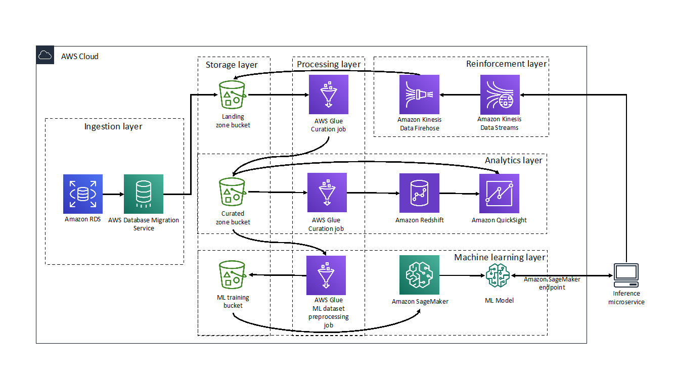





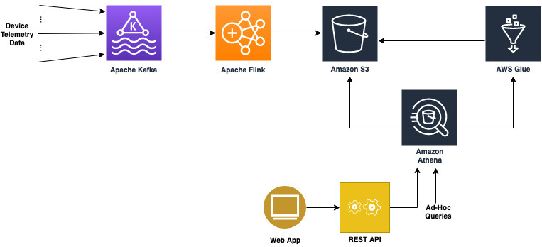
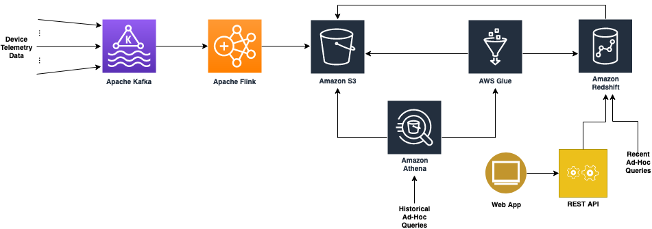



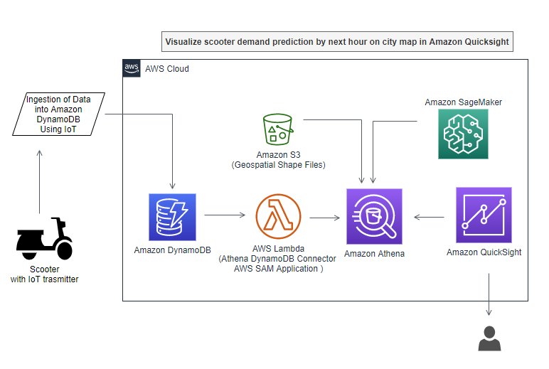



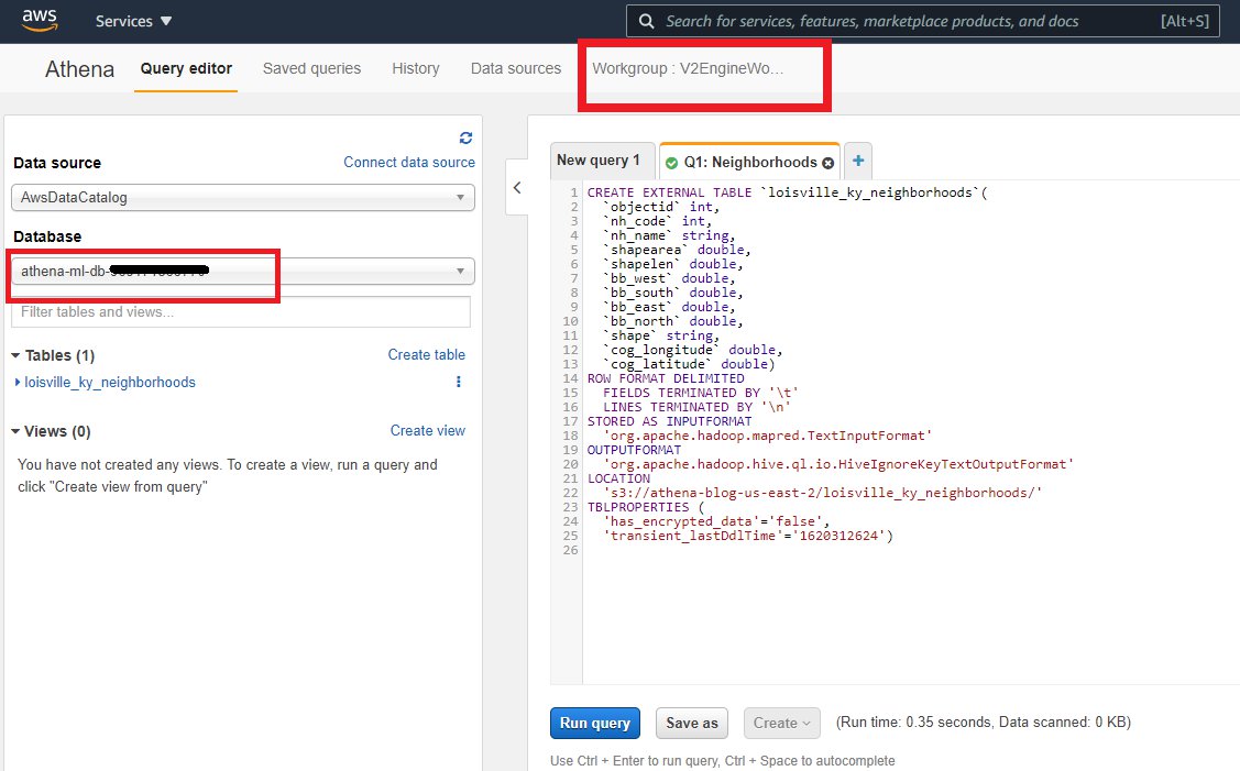
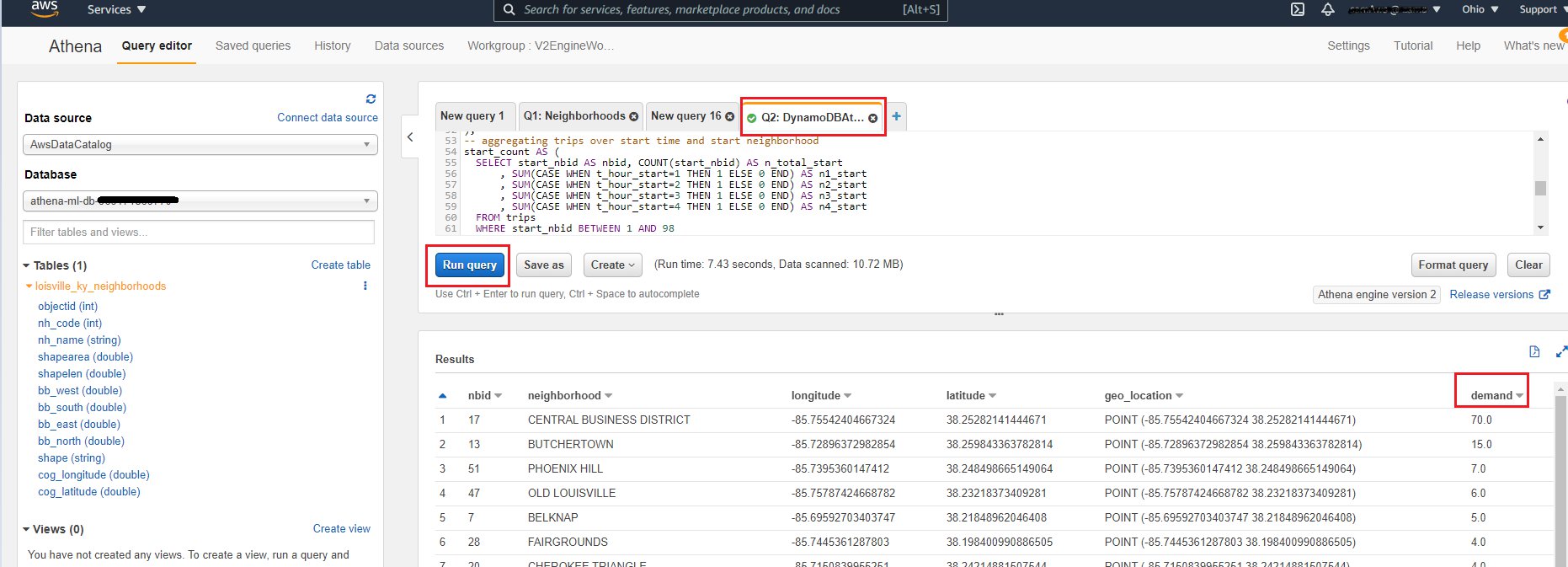


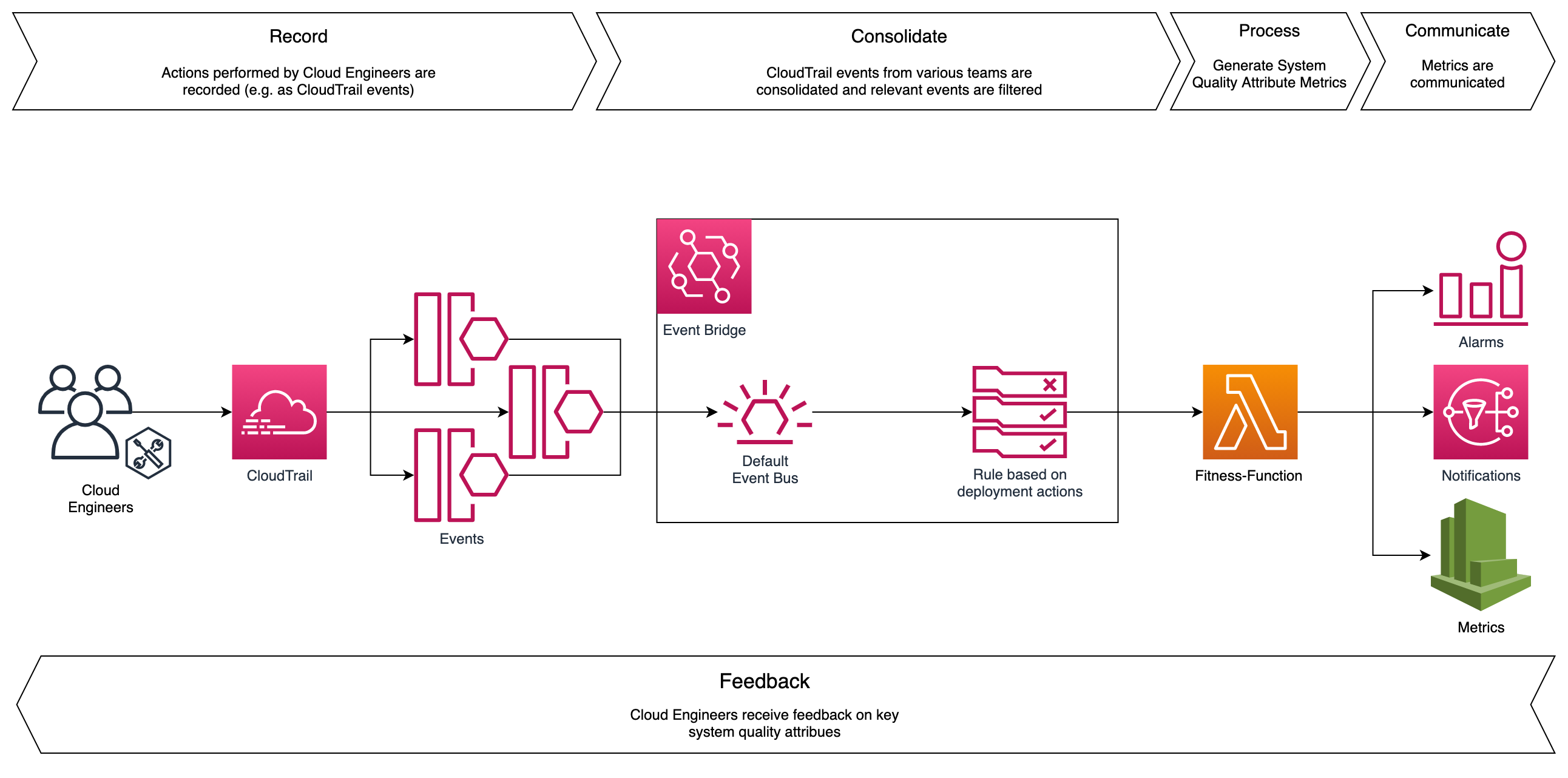
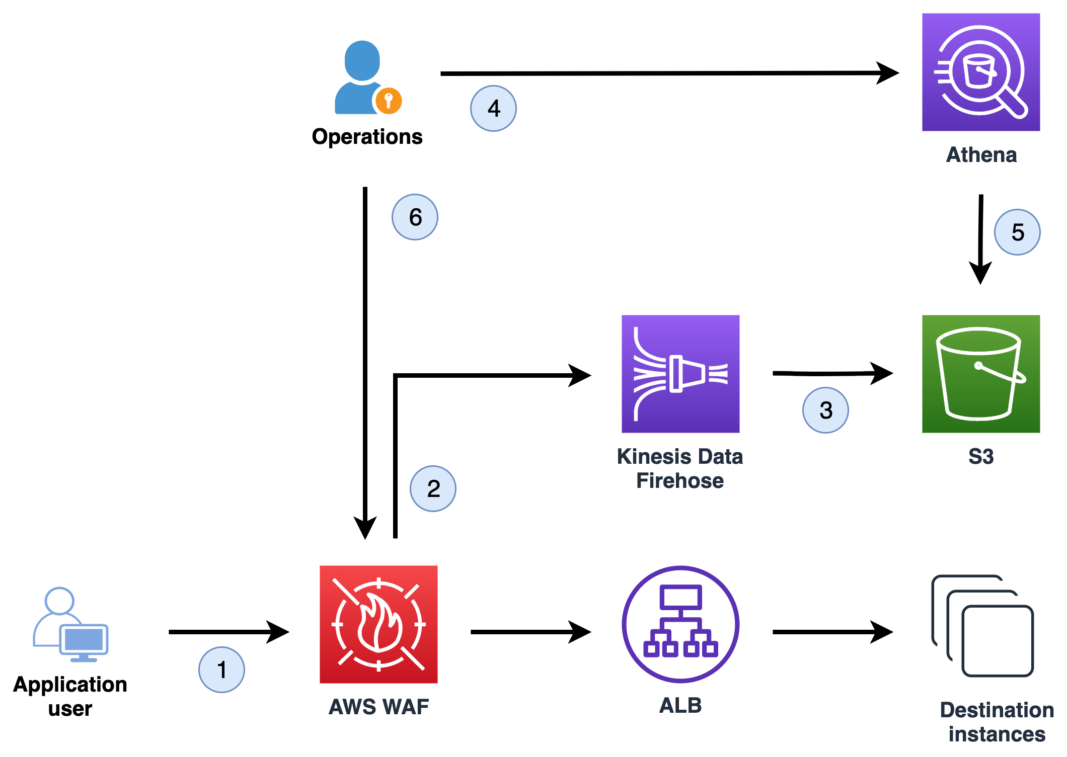
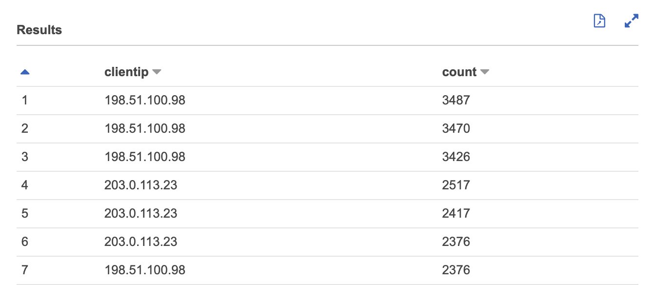
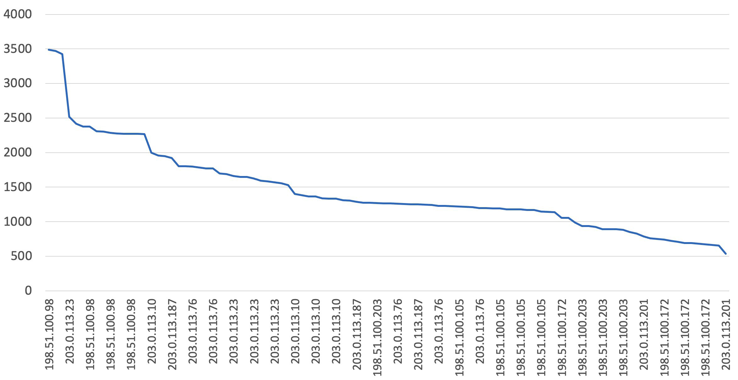
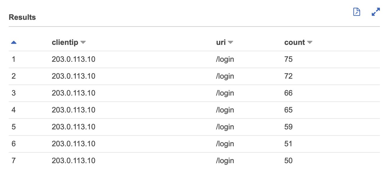
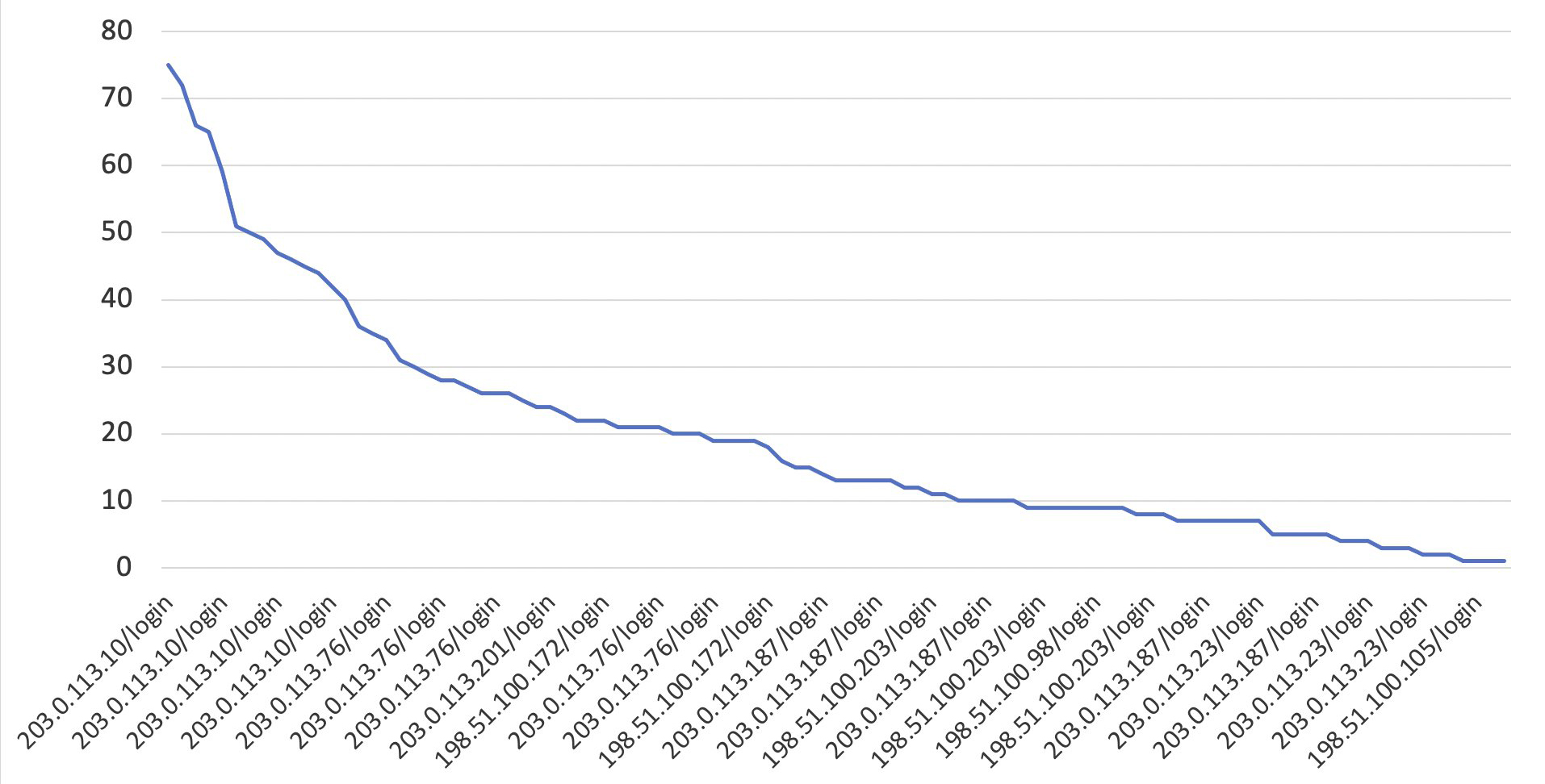
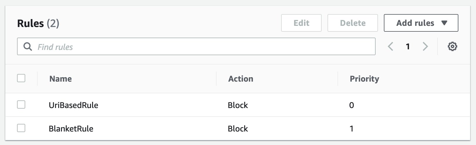
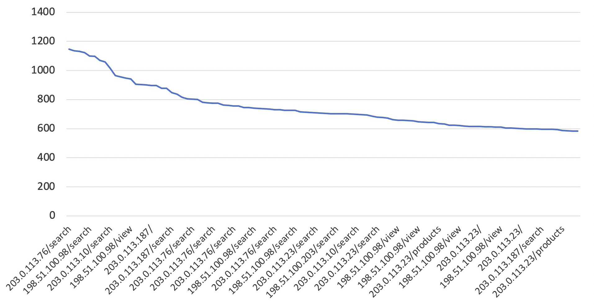


 Armando Segnini is a Data Architect with AWS Professional Services. He spends his time building scalable big data and analytics solutions for AWS Enterprise and Strategic customers. Armando also loves to travel with his family all around the world and take pictures of the places he visits.
 Xavier Naunay is a Data Architect with AWS Professional Services. He is part of the AWS ProServe team, helping enterprise customers solve complex problems using AWS services. In his free time, he is either traveling or learning about technology and other cultures.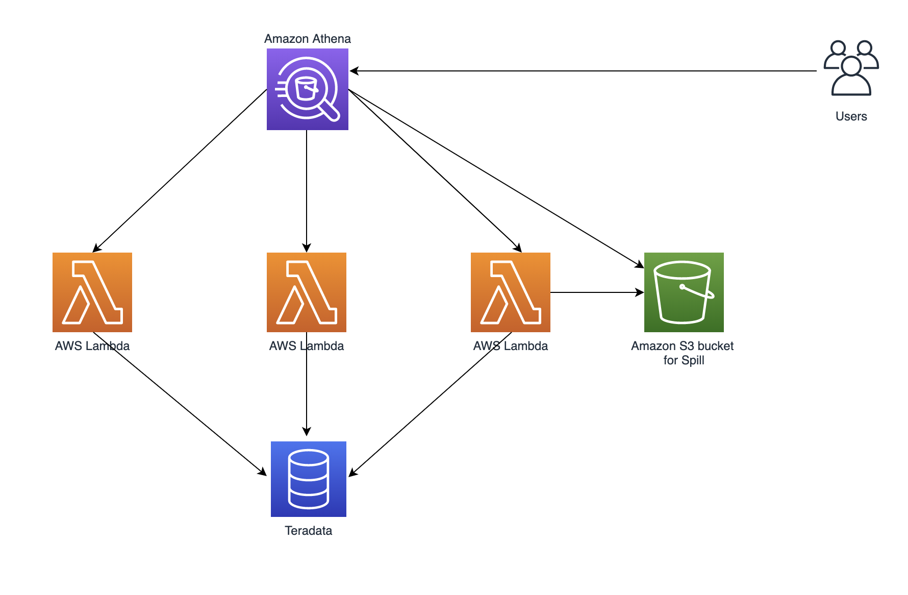
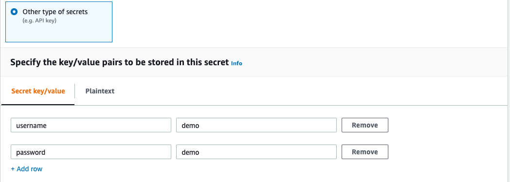
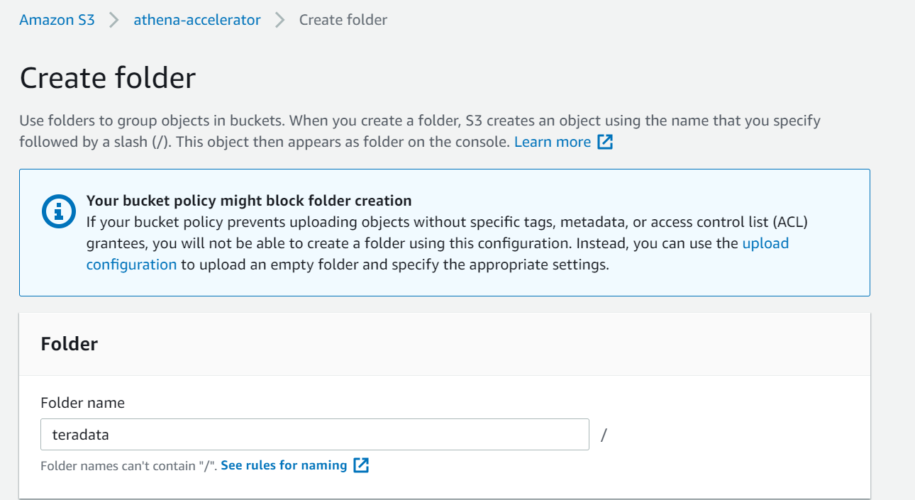
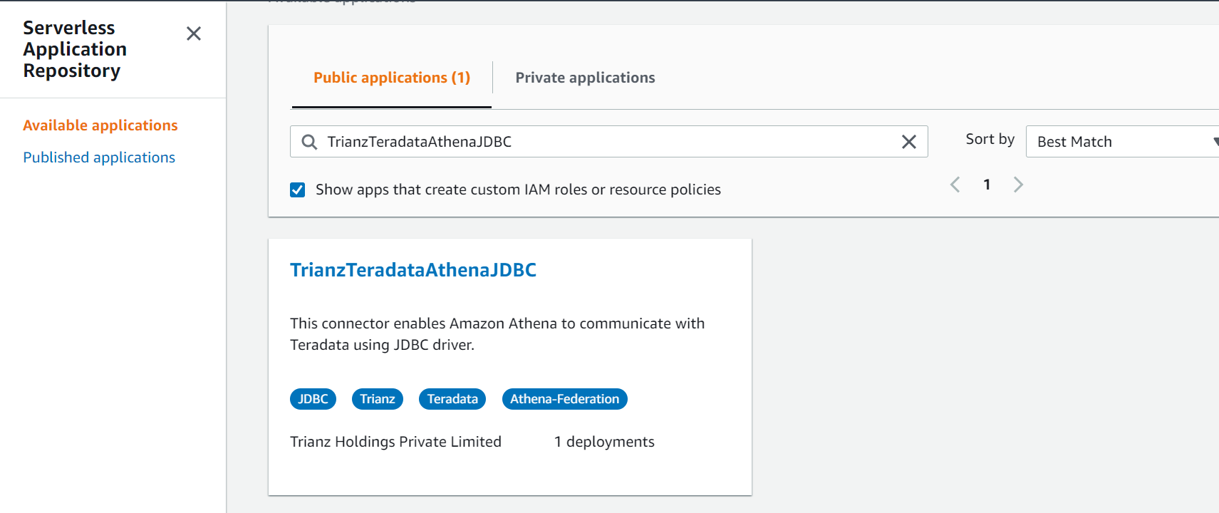
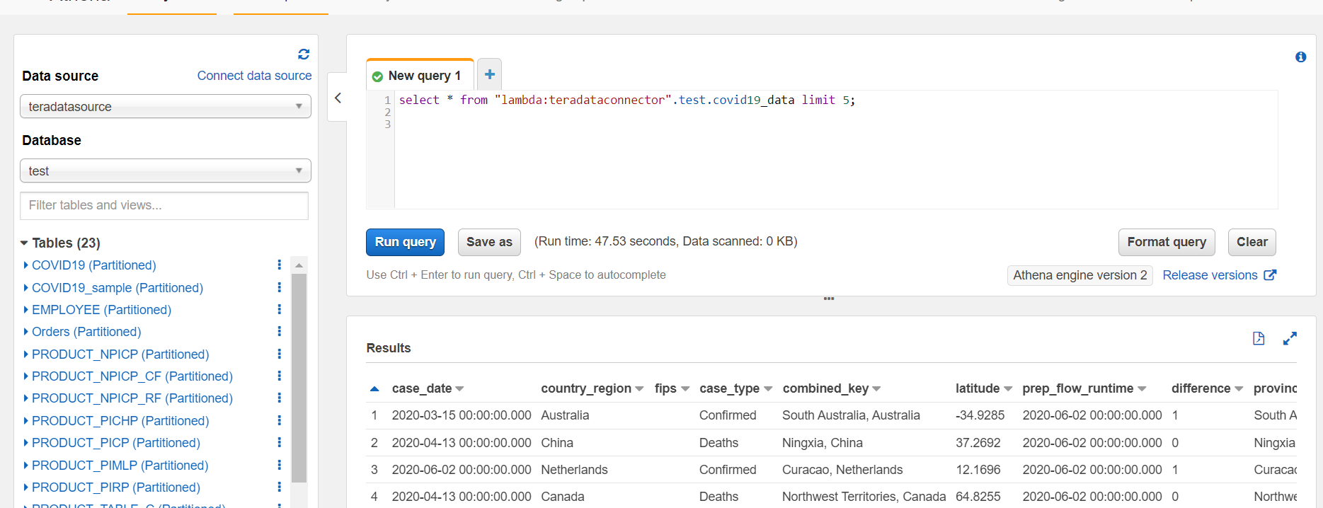
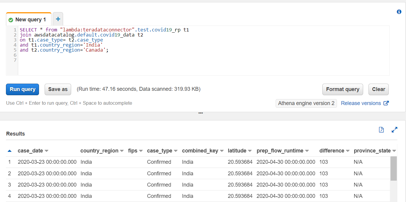
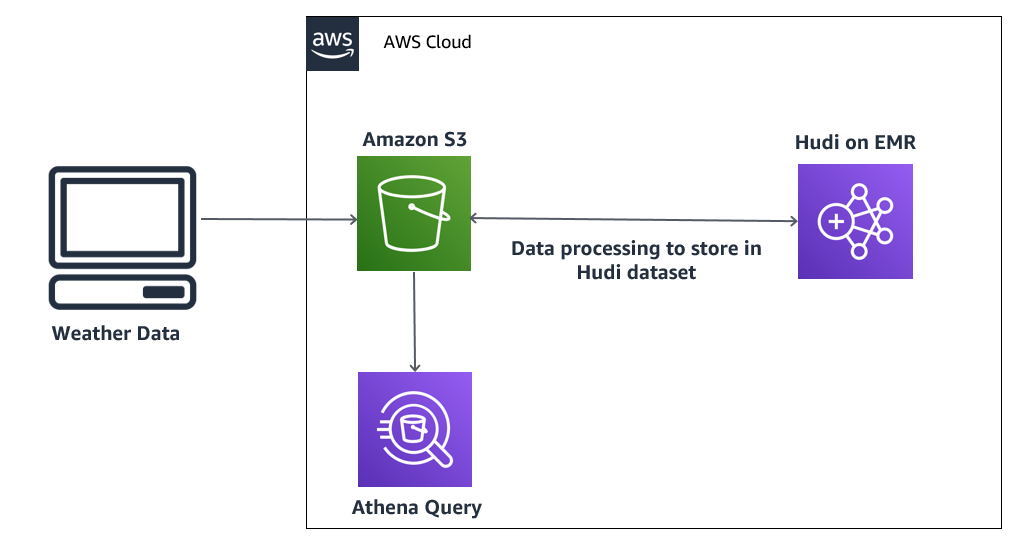
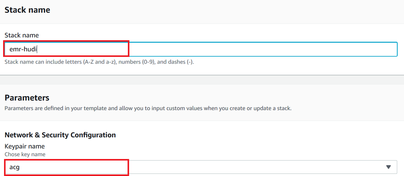
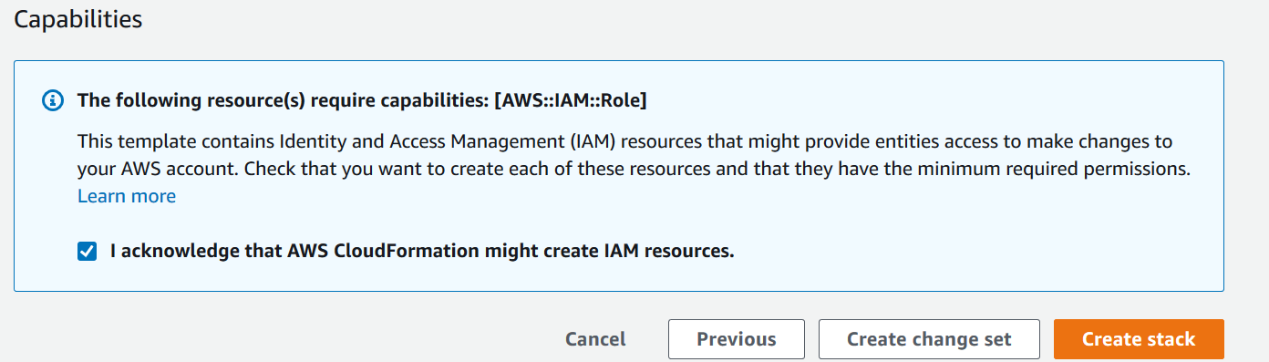






 Dhiraj Thakur is a Solutions Architect with Amazon Web Services. He works with AWS customers and partners to provide guidance on enterprise cloud adoption, migration and strategy. He is passionate about technology and enjoys building and experimenting in Analytics and AI/ML space.
 Sameer Goel is a Solutions Architect in The Netherlands, who drives customer success by building prototypes on cutting-edge initiatives. Prior to joining AWS, Sameer graduated with a master’s degree from NEU Boston, with a Data Science concentration. He enjoys building and experimenting with creative projects and applications.
 Imtiaz (Taz) Sayed is the WW Tech Master for Analytics at AWS. He enjoys engaging with the community on all things data and analytics.